Breaking moraine dams by catastrophic erosional incision

Rachel Zammett

March 15, 2007

1 Introduction

Glacial lakes occur in many mountainous areas of the world, such as the European Alpsor the Cordillera Blanca mountain range in north-central Peru. Here we consider thoseglacial lakes that were formed during the period of glacier retreat that followed the end ofthe Little Ice Age (figure 1). Such lakes are typically up to a kilometre long, hundreds ofmetres wide and up to a hundred metres deep and are often dammed on at least one sideby moraine (sediment deposited by a glacier).

Figure 1: Schematic diagram of a glacial lake, taken from Clague and Evans [2]. Theupper (grey) glacier surface is that of a long, thick glacier that would have advanced duringthe Little Ice Age. When this period of cool climate ended, glaciers retreated rapidly andsubstantially; such a thin, retreating glacier is labelled ‘modern day glacier’. It is during aperiod of glacier retreat that a glacial lake is typically formed. The moraine dam is shownat the right of the picture. If the toe of the retreating glacier (which is often unstable andheavily crevassed) suddenly deposits a large amount of ice into the lake, a displacementwave which can overtop the dam is initiated.

Moraine dams fail in two main ways. As glacial lakes are often located in steep alpine

162

valleys (where avalanches and rockfalls are common), or beneath the unstable toe of aretreating glacier, there is the possibility that a large amount of ice or rock may suddenlyfall into the lake. This initiates a displacement wave: one such rock avalanche in Perudeposited O(106) m3 of rock in glacial lake Safuna Alta, and initiated a displacement waveestimated to be over 100 m high [8]; more generally, it is estimated that avalanches typicallycreate displacement waves up to 10 m high [4]. Such a displacement wave can overtop themoraine dam and erode its downstream face.

In general, however, we have seen experimentally that one such overtopping wave doesnot cause the dam to fail. Instead, we observed that some of the initial wave is reflectedback into the lake, leading to the formation of a seiche wave (a standing wave in an enclosed,or partially enclosed, body of water). Such waves are often observed to occur naturally inharbours due to tidal influence, for example [13].

The subsequent reflected waves can also overtop the dam, and it is these repeatedovertopping events and associated erosion of the dam that lead to the incision of a channelon the downstream face of the dam. If such a channel is eroded to a sufficient depth quicklyenough, it becomes a conduit through which the lake can drain; it is this mechanism of lakedrainage that we term ‘catastrophic erosional incision’.

Evidence for more than one overtopping event has been seen in several such drainagefloods [9], and the possibility of a ‘series’ of waves was identified by Costa and Schuster[4]. The only mention in the literature of a seiche wave in connection with dam failure isfound in Hubbard et al. [8], where examination of a moraine dam after a rockfall-initiateddisplacement wave indicated at least ten reflected waves. We show here how the reflectedwaves play a crucial role in the failure of the dam.

The other mechanism by which a moraine dam can break is that of gradual overtopping,whereby the lake water level slowly increases until the water overtops and then breachesthe dam. Such a water level rise can be caused by excessive snowmelt or rainfall: themoraine which dammed Lake Tempanos in Argentina failed in the 1940s due to meltwateraccompanying a 350 m glacier retreat [16].

Drainage of a glacial lake can release O(106) m3 of water and have a peak discharge of103–104 m3 s−1 [2]. As the subsequent floodwater moves down valley, it entrains sedimentand can form a debris flow. One such debris flow, initiated by a glacial lake flood in Peruin 1941, devastated the city of Huaraz, killing over 6000 people [5]. While the majority ofsuch floods occur in remote, uninhabited valleys, these locations are now often consideredfor recreation, tourism and as sites for hydro-electric power stations, for example. Thusunderstanding the hazards associated with such a flood is of prime importance.

In this project, there are two main issues we will address. Firstly, we shall considerthe threshold behaviour of the phenomenon - why didn’t the moraine dam break in thecase of Laguna Safuna Alta, despite an initial wave 100 m high and at least ten subsequentseiche waves? We also consider how to estimate the peak discharge from such a catastrophicdrainage event, as this can be used as a measure of how destructive the resulting flood willbe.

163

2 Experiments

We performed a series of experiments over the summer, both as a qualitative explorationof the phenomenon and to quantify some of the theoretical results outlined in Section 3below. In all cases we used the experimental setup shown in figure 2: a rectangular glasstank with length 125 cm, width 20 cm and depth 30 cm. This was open at one end (theright hand end in figure 2), so that sediment and water could drain from the tank. At theopen end, we built a sediment dam. This dam was approximately 10 cm high and 40 cmwide at the base and was made using a mould to endeavour to keep the dams uniform inshape. The tank was then filled with water, and the experiment was left until water hadseeped through the entire dam. A single wave was then initiated at the left hand end of thetank; this was to simulate the displacement wave initiated by a rockfall or avalanche.

Figure 2: Experimental setup.

Sediment properties

We used four different sediments in the dambreak experiments. These were grit and threetypes of sand with different particle size distributions. The properties of these sediments(when dry) are summarised in Table 1.

Glacial moraine is characterized by a wide range of particle sizes, from fine clays to largeboulders. This sediment is poorly sorted and loosely consolidated; lake drainage typicallyoccurs by seepage through the dam. Clarke [3] shows an example of moraine from Trapridgeglacier with a bimodal particle size distribution; this is a feature of many moraines. In orderto reproduce such a bimodal particle size distribution, we therefore made two mixtures ofsand and grit. The properties of these mixtures (when dry) are summarised in Table 2.

The sediments and their properties will also be discussed in Section 3 below, where weconsider the erosion of the dam.

164

Sediment ρ (103 kg m−3) Porosity Repose Modal particle size (µm)

Caribbean Sand N/A N/A N/A 250Florida Sand 2.34 0.38 39◦/34◦ 310Beach Sand 2.34 0.35 40◦/33.5◦ 950

Grit 2.42 0.42 37◦/28◦ 1150

Table 1: Properties of individual sediments when dry. Sediment density was calculatedfrom the weight of a given sediment volume once the sediment porosity was determined.Sediment porosity was measured by measuring how much water was absorbed by a givenvolume of sediment. The column headed ‘Repose’ shows the angles of repose of the drysediment; the first value is the angle of repose associated with tilting a pile of sediment, thesecond that associated with creating a conical pile of the sediment. The differing values aredue to the bistability of the system [11]. Modal particle size was estimated from particlesize distributions which were obtained by laser diffraction. Some of the properties of theCaribbean sand were not determined.

Mixture Composition ρ (103 kg m−3) Porosity Repose

1 Caribbean Sand/Grit 2.38 0.32 38.5◦/33◦

2 Florida Sand/Grit 2.36 0.37 44◦/34◦

Table 2: Properties of sediment mixtures, determined as in Table 1. As the mixtures arebimodal by design, we have omitted the modal particle size column.

2.1 Results

Here we consider results from qualitative experiments. We first consider the results ofexperiments using the individual sediments, some of which are shown in Table 3. We seethat grit alone makes a poor dam - its high porosity means that the lake drains out rapidly,and thus makes the dam unstable. It is also difficult to incise a channel in the downstreamface because overtopping water simply seeps into the dam rather than eroding it. In contrast,the sands are, in general, better in terms of ease of channel incision. However, they are alsoprone to slumping when wet, indicating that they would make a poor dam; sand dams wereoccasionally observed to break before a wave was initiated.

Some of the results for the sediment mixtures are shown in Table 4. Although it isnot clear from this table that dams constructed from the sediment mixtures were easier tobreak by catastrophic incision than those made from the individual sediments, they werequalitatively observed to be better in terms of both initial dam stability and ease of channelincision. These observations lead to the conclusion that it is perhaps the composition ofmoraine that leads such dams to fail via catastrophic erosional incision - the distributionof particle sizes both increases the dam stability, making the existence of a lake possible,and allows for easier channel incision. This may explain why the phenomenon is not seenin other natural dams, such as landslide dams for example.

165

Sediment 1 2 3 4

Play Sand 1/9 1/14 2/19 1/12Beach Sand 2/16 1/19 2/14 2/16

Grit X 1/6 X X

Table 3: Experimental results for the individual sediments. The columns show differentexperimental runs. The first number in each column is the number of waves that needed tobe initiated for dambreak. The second number is the total number of waves that overtoppedthe dam before incision occurred. The onset of incision is taken to be the point at whichthe lake drains independently of the action of the seiche wave. A cross denotes a dam whichdid not break.

Mixture 1 2 3 4

1 X 2/28 1/15 1/82 1/13 1/5 2/24 1/13

Table 4: Experimental results for the sediment mixtures. The table is laid out as Table 3above.

3 Theory

In this section, we split the problem in two. Firstly, we model the seiche wave in thelake using shallow water theory in one dimension. We then use a hydraulic model for thedambreak itself, before considering a unified theory to explain the interaction between theseiche wave and the dam.

3.1 Describing the seiche wave

We work in two dimensions, x and z. Water of velocity u = (u(x, z, t), w(x, z, t)) and depthh(x, t) flows over an erodible bed with elevation ζ(x, t) . We assume that the horizontalextent of the flow is much greater than its depth; the lake is much longer than it is deep.In this case, we have that ∂

∂z � ∂∂x , and thus the continuity equation implies that u � w.

Conservation of vertical momentum then implies that the pressure is hydrostatic to leadingorder, and irrotationality that u is independent of z.

We therefore write conservation of mass and horizontal momentum in the following form

ht + (hu)x = 0, (1)

ut + uux = −g(h + ζ)x − D(u, h) + νuxx, (2)

where u is the depth averaged velocity, given by

u =1

h

∫ h+ζ

ζu dz, (3)

and D(u, h) is a drag term which represents frictional effects, with the properties that

166

Figure 3: The co-ordinate system used in the shallow water theory.

∂D∂u > 0 and ∂D

∂h < 0; drag increases with velocity and decreases with depth. A full derivationof the shallow water equations may be found in Stoker [18], for example.

In fluvial systems, it is common to use the Chezy drag law, given by

D(u, h) = cfu|u|h

, (4)

where cf is the dimensionless Chezy drag coefficient. Typically, for a smooth watercoursesuch as a glass tank, cf = O(10−3) [1], while for a rough watercourse, such as a rocky alpinestream, it may be as large as 0.1 [6].

However, this formula is not appropriate to use in the context of our experiments, wherethe flow was observed to be laminar. In 1959, Keulegan determined that for a standing wavein a glass rectangular tank, the drag is primarily accounted for by laminar viscous boundarylayers on the tank walls and base [10]. This theory was later modified to account for theeffects of surface tension and surface contamination [12], but we shall consider these to besmall corrections.

To modify Keulegan’s linear theory for our purposes, we note that shallow water theorycan also be used in the boundary layers near the tank walls. Using the same arguments asabove, we write conservation of momentum as

ut = −1

ρpx + νuzz, (5)

and then, given that pz ≈ 0, we eliminate the hydrostatic pressure to obtain

uzt = νuzzz. (6)

We then pose a time periodic solution of the form u = f(z)eiωt (and consider only the realpart of this solution) to obtain

f = C + A±e±Kz, (7)

where A± and C are constants of integration, and K =

√

ω

2ν(1 + i). The boundary condi-

tions are

uz → 0, as z → ∞, (8)

u → u0, as z → ∞, (9)

u = 0, z = 0, (10)

167

0 10 20 30 40 50 60 700

0.01

0.02

0.03

0.04

0.05

0.06

0.07

0.08

0.09

0.1

Number of reflections

Sei

che

ampl

itude

(m)

Experimental resultsChezy dragLinear drag

Figure 4: Comparison of the Chezy and linear drag laws with experiment, where a seiche(standing) wave was initiated in a rectangular tank. The values used were cf = 0.001,ν = 1×10−6. We see that the linear drag theory (solid magenta line) is a much better fit tothe data than the nonlinear Chezy drag law (dashed line). Stars denote the experimentaldata.

where u0 is the flow velocity in the main body of fluid outside the boundary layer. Thesolution is therefore

u = u0eiωt(1 − e−Kz), (11)

and the vertical velocity gradient at the base is given by

uz|z=0= Ku0. (12)

In the shallow water equations for the main flow, we therefore have

ut + uux = −g(h + ζ)x −√

νω

2

u

h+ νuxx, (13)

where the drag term is now D(u, h) =√

νω2

uh . We set α =

√

νω2

; thus α has units of velocity.We illustrate the difference between the drag laws by comparing them with the results

from a simple laboratory experiment (figure 4), where a standing wave was initiated in aclosed, rectangular glass tank. Figure 4 shows that that the linear drag is a much better fitto the data than the Chezy drag; we therefore use linear drag in the theory that is to follow.However, we note that in a glacial lake where the Reynolds numbers are much higher, it islikely that the Chezy formula will be more appropriate.

We consider a lake with mean depth H(x), on which there is a seiche wave of amplitudeη(x, t), such that the total water depth is given by h(x, t) = H(x) + η(x, t). Equations (1)

168

and (2) then become

ηt + [(H + η)u]x = 0, (14)

ut + uux = −g(H + η + ζ)x − αu

h+ νuxx. (15)

We now nondimensionalise using the following scales

t ∼ 1

ω, u ∼ U, η ∼ N, H ∼ H0, h ∼ H0, ζ ∼ H0, x ∼ L, (16)

where ω is the frequency of the seiche wave. Equations (14) and (15) become

ωNηt +UH0

L[(H + εη)u]x = 0, (17)

ωUut +U2

Luux = −gH0

L(H + εη + ζ)x − α

U

H0

u

H + εη+ ν

U

L2uxx, (18)

where ε = NH0

� 1. To retain a balance in equation (17), we choose U = εωL, and weassume that (H + ζ)x = 0, i. e. the undisturbed free surface is flat, to obtain,

ηt + (Hu)x = −ε(ηu)x, (19)

ut + βηx = −εuux − εαu

H + εη+ ενuxx, (20)

where the dimensionless parameters are given by

β =gH0

ω2L2, α =

α

ωH0

, ν =ν

ωL2, (21)

and we have rescaled the drag and viscosity terms with ε; i. e. we have assumed that theyare small.

We now assume that there are a fast and a slow timescale in the problem, such that∂∂t = ∂

∂t+ ε ∂

∂T . On dropping the ˆ, equations (19) and (20) become

ηt + (Hu)x = −ε(ηu)x − εηT , (22)

ut + βηx = −εuux − εαu

H + εη+ ενuxx − εuT . (23)

We now pose expansions in the form u ∼ u0 + εu1 + . . . and η ∼ η0 + εη1 + . . .. To leadingorder, equations (22) and (23) are

η0t + (Hu0)x = 0, (24)

u0t + βη0x = 0. (25)

Differentiating equation (24) with respect to time and using equation (25), we obtain thesingle equation for the wave height, η:

η0tt = β(Hη0x)x. (26)

169

In the simple case of a rectangular tank of constant depth H0 and width L, such that thescaled boundaries are at x = 0 and x = 1, (where we require the velocity to vanish, soηx = 0 if we assume time periodic solutions), there are solutions of the form

η = Aeit cos

(

x√β

)

, (27)

where we require π =√

β, i. e. ω = π√

gH0

L . In dimensional terms, the solution for η is

η = Aeiωt cos(πx

L

)

. (28)

This first approximation to the behaviour of the seiche wave will be used in Section 3.3below.

Numerical solutions for a given basal topography

It is possible to solve equation (26) numerically for a given basal topography, if we againassume time periodic solutions. We replace the right hand boundary, previously a verticaltank wall, by a non-erodible dam of prescribed shape, so that dimensionlessly H = 0 atx = 1. As this is an eigenvalue problem, we require three boundary conditions. On theleft boundary, x = 0, we require that u = 0. At x = 1 (where H = 0) we require that thesolution is regular. For the case of a uniformly sloping base, an analytic solution may befound in terms of Bessel functions, such that η ∼ J0(x

1/2) [19]. This analytic solution isshown in figure 5. We set y = 1 − x, such that close to x = 1,

η ∼ J0[(1 − y)1/2] ∼ 1 + O(1 − y). (29)

To ensure we obtain a regular solution, we therefore require that η = 1 at x = 1. We notethat near x = 1, H ∼ −(1 − x)H ′

∗, where H ′∗ = H ′|x=1

. Again setting y = 1 − x, we useequation (26) to write

−ω2η = βH ′∗(

yη′)′

, (30)

which gives, to leading order,ω2η = βH ′

∗η′. (31)

The three boundary conditions are therefore

η = 0 on x = 0, (32)

η = 1 on x = 1, (33)

ω2η = βH ′∗η

′ on x = 1. (34)

Note that if H ′∗ = 0, the problem is ill-posed, as boundary conditions (33) and (34) then

imply both η = 0 and η = 1 at x = 1. A numerical solution of equation (26) with boundaryconditions (32) – (34) for a dam of Gaussian shape is shown in figure 6.

170

0 0.2 0.4 0.6 0.8 1−1

−0.8

−0.6

−0.4

−0.2

0

0.2

0.4

0.6

0.8

1

x

Hei

ght r

elat

ive

to in

itial

wat

er le

vel

Figure 5: Numerical result for a uniformly sloping bed, with initial water depth given byH(x) = 1−x. The upper solid line is the water surface, the lower line the basal topography.The dashed line indicates the initial water level.

0 0.2 0.4 0.6 0.8 1 1.2 1.4−1

−0.8

−0.6

−0.4

−0.2

0

0.2

0.4

0.6

0.8

1

x

Hei

ght r

elat

ive

to in

itial

wat

er le

vel

Figure 6: Numerical result for a uniformly sloping bed, with initial water depth given byH(x) = 1− 1.1 exp

(

−(x − 1.05)2/(2 × 0.12))

. The upper solid line is the water surface, thelower line the basal topography. The dashed line indicates the initial water level.

Higher order terms

We consider solutions of equation (26) of the form

(η0, u0) = (N, iU)A(T )eiωt + c.c., (35)

171

thus N,U are real. Equations (24), (25) and (26) then become

ωN = −(HU)x, (36)

U = βNx, (37)

−ω2N = β(HNx)x, (38)

with solutions as above. To the next order in ε, we then have

η1t + (Hu1)x = −(η0u0)x − η0T , (39)

u1t + βη1x = −u0u0x − αu0

H+ νu0xx − u0T . (40)

We now use equation (35) to write equations (39) and (40) in terms of N and U ;

η1t + (Hu1)x = −iA2NUe2iωt − AT Neiωt + c.c. (41)

u1t + βη1x = A2UUxe2iωt − 2AA∗UUx − αiAUeiωt

H+ iνAUxxe

iωt − iAT Ueiωt + c.c..(42)

We can find particular solutions to remove any terms on the right hand sides of equations(41) and (42) which are not multiples of eiωt. The remaining parts which are proportional toeiωt are potentially secular in time, and must therefore be removed in order to find a uniformasymptotic approximation over the fast time t. Discarding the non-secular inhomogeneousterms, and assuming that η1 = η1(x)eiωt and u1 = u1(x)eiωt, the system we therefore lookto solve is

iωη1 + (Hu1)x = −AT Neiωt (43)

iωu1 + βη1x = −αiAUeiωt

H+ iνAUxxeiωt − iAT Ueiωt. (44)

Equations (43) and (44) may be rewritten as

iωη1 + (Hu1)x = I1, (45)

iωu1 + βη1x = I2, (46)

where

I1 = −AT N, (47)

I2 = −αiAU

H+ iνAUxx − iAT U. (48)

We combine equations (45) and (46) to obtain

ω2η1 + β (Hη1x) = −iωI1 + (HI2)x, (49)

and then integrate equation (49) with respect to x. After integrating by parts and usingthe seiche equations (36) and (37), we obtain

∫

1

0

N [−iωI1 + (HI2)x] dx = 0, (50)

172

which can be simplified using equations (47) and (48) to give

−2AT

∫ 1

0

ωN2 dx + αA

∫ 1

0

NUx dx + νA

∫ 1

0

N(HUxx)x dx = 0. (51)

This then gives a solution of the form A = A0e−γT , where γ is evaluated numerically using

equation (51). The calculation can be repeated for dissipative terms given by Chezy dragand viscosity, yielding

AT

∫

1

0

ωN2 dx = −νA

∫

1

0

N(HUxx)x dx +4A|A|cf

π

∫

1

0

N(U |U |)x dx. (52)

Again, the integrals in equation (52) may be evaluated numerically for any given basaltopography H(x), and this allows the relative importance of the dissipative terms to bequantified.

3.2 Modelling the dambreak

Erosion

The flux of sediment is governed by a (dimensionless) critical value of the Shields stress,defined by

τ∗ =u2∗

RgD, (53)

where R = ρs−ρl

ρlis the specific gravity, D is a typical particle diameter and u∗ is the

threshold velocity, which is particular to the sediment and is determined empirically. Theidea is that the fluid flow needs to exceed the threshold velocity in order to exert enoughshear stress at the base to lift particles into suspension and thereby erode the bed.

We follow Parker [20], [21] and use the following empirical, dimensionless erosion law

E(u) =

{(

u2

u2∗

− 1)1.5

for u > u∗,

0 for u < u∗.(54)

A law of this type captures the two important features of any erosion law: below a certainthreshold, there is no erosion, and for large values of the Shields stress (or velocity, in thiscase), erosion has a power law behaviour. The exponent in equation (54) is again empiricallydetermined and, while not universally agreed upon, it is common to use the value 1.5 [14].

In fluvial systems, the Exner equation (conservation of sediment) is commonly used tomodel the erosion of the dam (which has elevation ζ(x, t)),

(1 − λp)∂ζ

∂t+

∂qs

∂x= 0, (55)

where λp is the sediment porosity and qs is the sediment flux, which is again determinedempirically as a function of the Shields stress.

However, it is also possible to consider the evolution of the dam height to be the neteffect of erosion and deposition,

∂ζ

∂t= −wE(u) + wsC, (56)

173

where the first term on the right hand side of equation (56) represents erosion and thesecond represents deposition. w is a sediment-dependent constant with units of velocity, ws

is a particle settling velocity, and C is a depth-averaged volumetric sediment concentration.Equation (56) must then be supplemented with an equation to describe the evolution of C,and it is usual to use an advection-diffusion equation, moderated by erosion and deposition,thus

h(Ct + uCx) = κhCxx + wE(u) − wsC, (57)

where κ is the sediment diffusivity. As a first approximation, we assume there is no depo-sition; thus we eliminate C and simply use

∂ζ

∂t= −wE(u). (58)

We calculated w experimentally using equation (58), and performing erosion experimentswhere we measured the dam height, ζ (at a fixed point in space as a function of time), andthe flow velocity u. We followed Parker [14] and calculated u∗ using the following empiricalrelationship for τ∗

τ∗ = 0.5[

0.22Re−0.6p + 0.06 × 10−7.7Re−0.6

p

]

, (59)

where Rep is the particle Reynolds number, defined as

Rep =(RgD)1/2 D

ν. (60)

Equation (59) coupled with equation (53) allows estimation of u∗ and thus w. Typical valuesfor the sediments used experimentally are given in Table 5. It is much more complicated toestimate sediment parameters for a mixture of sediments, and so this was not attempted.For calculations involving particle diameter (such as estimation of the particle Reynoldsnumber), the modal particle size was used.

Sediment Rep τ∗ u∗ (m s−1) w (m s−1)

Play sand 20 0.0198 9 ×10−3 9.6 × 10−9

Beach sand 107 0.0169 1.5 × 10−2 4.7 × 10−8

Grit 147 0.0179 1.7 × 10−2 4.9 × 10−8

Table 5: Empirically and experimentally determined sediment properties.

Hydraulic Control

We now use a hydraulic model coupled with erosion to describe the dambreak. Hydraulicmodels are commonly used to describe stratified flows over sills in the ocean, see Pratt [15],for example. The benefit of using such a model is that at one or more locations in thesystem the flow adjusts to a well-defined state; i. e. it is in some sense ‘controlled’ by thiscritical point. Here, the location of hydraulic control will be the point at which the damheight is a maximum.

174

Hydraulic control theory also assumes steady flow. From equation (58), we have thatthe timescale over which erosion occurs is tE ∼ H

wE0. Using typical values from Table 5,

u∗ = 1 × 10−2 m s−1 and w = 5 × 10−8 m s−1, and a typical experimental value H = 0.1m, we estimate that tE ≈ 100 s. This implies that for the dambreak ∂

∂t � 1, and we cantherefore neglect the time derivatives in the shallow water equations (1) and (2). As a firstapproximation, we also neglect drag and viscosity (although it is possible to include thesein the description, see Pratt [15], Hogg and Hughes [7]).

We can therefore integrate the equations for conservation of mass and momentum withrespect to x to obtain

q = hu, (61)

1

2u2 + g(h + ζ) = B, (62)

where q is the constant water flux (with units m2 s−1) and B is the energy, sometimesreferred to as the Bernoulli constant.

We consider the problem of a reservoir of depth H and length L, which must drain overa dam of maximum height ζm. Here, the subscript m will be used to denote evaluation ofa function at this maximum of ζ; thus um is the flow velocity at the highest point of thedam. We assume that the dam has finite width, and thus ζ = 0 outside some finite region.We can therefore use equations (61) and (62) to write

B =1

2

q2

H2+ gH ≈ gH, (63)

if we assume that the depth of the reservoir is much greater than the depth of the waterflowing over the dam, i. e. H � h. Using equation (61), we may write the non-integratedmomentum equation in the form

ux =−gζxu2

u3 − gq, (64)

and thus for the velocity gradient to be defined at all points in the system, we require thatu3 = gq at the point where ζx = 0; i. e. where ζ = ζm. We therefore obtain

um = (gq)1

3 , hm =q

um=

(

q2

g

)

1

3

. (65)

Note that we can use the expressions in equation (65) to write the Bernoulli constant as

B =3

2u2

m + gζm. (66)

Equations (63) and (66) allow us to relate upstream variables to those at the maximumheight of the dam,

gH =3

2u2

m + gζm. (67)

To complete the system, we couple equations (61) and (62) with equations describing thedrainage of the lake,

LdH

dt= −q, (68)

175

and the erosion of the dam,∂ζ

∂t= −wE(u). (69)

Nondimensionalisation

We nondimensionalise the system of equations (61), (62), (68) and (69) using the followingscales

u ∼ u0, h ∼ h0, H ∼ H0, ζ ∼ H0, t ∼ t0, q ∼ q0, E ∼ E0. (70)

and thus obtain(

q0

h0u0

)

q = hu, (71)

1

2

u20

gH0

u2 +

(

h0

H0

)

h + ζ = B∗, (72)

(

LH0

q0t0

)

dH

dt= −q, (73)

(

H0

wt0E0

)

∂ζ

∂t= −E(u), (74)

where B∗ is the dimensionless Bernoulli constant.We make the choices q0 = h0u0, and as we are interested in the timescale over which

erosion occurs, we choose t0 = H0

wE0. Equations (71) – (74) then become

q = hu, (75)

1

2F 2α2u2 + αh + ζ = B∗, (76)

µdH

dt= −q, (77)

∂ζ

∂t= −E(u2), (78)

where the dimensionless parameters are the Froude number, F 2 =u2

0

gH0, the ratio of the

water height at the dam peak to the reservoir height, α = h0

H0, and a measure of how

quickly erosion occurs relative to lake drainage, µ = wLE0

q0. We now make the further

choices h0 = H0 and u0 =√

gH0, such that α = F 2 = 1.The dimensionless form of the erosion law (equation (61)) is

E(u) = (u2 − δ3)1.5+ , (79)

where E0 =

(

u0

u∗

)3

, δ =u∗u0

and the subscript + indicates that E = 0 when the quantity in

the brackets is less than zero.We take typical experimental values: H0 = 0.1 m, w = 5×10−8 m s−1, L = 1 m, u0 = 1

m s−1 and u∗ = 1 × 10−2 m s−1, to obtain

µ = 0.5, δ = 10−2, E0 = 1 × 105. (80)

Again, we estimate t0 = 100 s, which should be both the timescale for erosion and for lakedrainage in our experiments (as µ is O(1)).

176

Figure 7: Schematic diagram of the two domains under consideration: a lake of length Land depth H adjacent to a dam of width σ and height ζ, such that σ � L and, initially,H ∼ ζm.

3.3 Unified theory: spatially distributed dam

In order to combine the theory of the seiche wave (outlined in Section 3.1) with the hydraulicmodel, we consider the following configuration, shown in figure 7: a rectangular lake oflength L and mean level H(t), on which there is a seiche wave of amplitude η(x, t). Thelake is adjacent to a dam of height ζ(x, t) and width σ, where σ � L.

We now revisit the scalings used Sections 3.1 and 3.2. In the lake,

h = H + εη, t ∼ 1

w∼

√gH0

L, x ∼ L, u ∼ ε

√

gH0, (81)

while over the dam,

t ∼ H0

wE0

, x ∼ σ, u ∼√

gH0. (82)

We impose the condition that the timescale in the lake must be of the same order as thatover the dam. However, we note that velocities in the lake are O(ε) smaller than those overthe dam, which means that the dam ‘sees’ the seiche wave as a gradual change in waterdepth, to which it can adjust instantaneously. We also note that x derivatives are muchlarger over the dam than in the lake.

We assume that there is a right hand boundary of the lake which lies close to theedge of the dam, x = xσ−, such that ζ(xσ−, t) = 0. We consider the water height at thisfixed point, given dimensionally by h(xσ−, t) = H(xσ−, t) + η(xσ−, t), and we suppose thatη(xσ−, t) = η(t) satisfies the ordinary differential equation

η + γη + ω2η = 0, (83)

where γ = αH is the damping coefficient calculated in Section 3.1, and ω(H) is the seiche

frequency. As we assume that the lake is a rectangular basin, we have that ω =π√

gH

Land

thus γ = γ(H).

177

0 10 20 30 40 500.06

0.07

0.08

0.09

0.1

0.11

Hei

ght (

m)

0 10 20 30 40 50−0.04

−0.02

0

0.02

0.04

Time (s)

Sei

che

ampl

itude

(m)

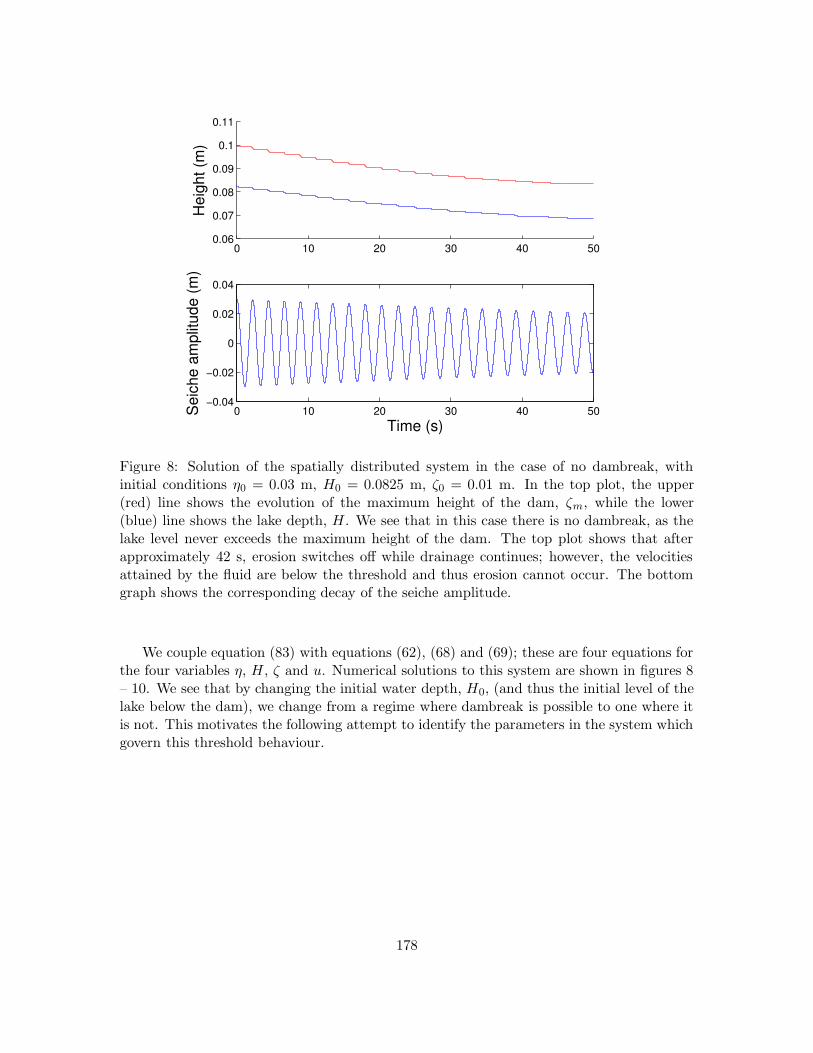
Figure 8: Solution of the spatially distributed system in the case of no dambreak, withinitial conditions η0 = 0.03 m, H0 = 0.0825 m, ζ0 = 0.01 m. In the top plot, the upper(red) line shows the evolution of the maximum height of the dam, ζm, while the lower(blue) line shows the lake depth, H. We see that in this case there is no dambreak, as thelake level never exceeds the maximum height of the dam. The top plot shows that afterapproximately 42 s, erosion switches off while drainage continues; however, the velocitiesattained by the fluid are below the threshold and thus erosion cannot occur. The bottomgraph shows the corresponding decay of the seiche amplitude.

We couple equation (83) with equations (62), (68) and (69); these are four equations forthe four variables η, H, ζ and u. Numerical solutions to this system are shown in figures 8– 10. We see that by changing the initial water depth, H0, (and thus the initial level of thelake below the dam), we change from a regime where dambreak is possible to one where itis not. This motivates the following attempt to identify the parameters in the system whichgovern this threshold behaviour.

178

0 0.2 0.4 0.6 0.8 10

0.050.1

t=400 s

0 0.2 0.4 0.6 0.8 10

0.050.1

t=600 s

0 0.2 0.4 0.6 0.8 10

0.050.1

t=2400 s

0 0.2 0.4 0.6 0.8 10

0.050.1

t=2544 s

0 0.2 0.4 0.6 0.8 10

0.050.1

t=0 s

0 0.2 0.4 0.6 0.8 10

0.050.1

t=200 s

0 0.2 0.4 0.6 0.8 10

0.050.1

t=800 s

0 0.2 0.4 0.6 0.8 10

0.050.1

t=1000 s

0 0.2 0.4 0.6 0.8 10

0.050.1

t=1200 s

0 0.2 0.4 0.6 0.8 10

0.050.1

t=1400 s

0 0.2 0.4 0.6 0.8 10

0.050.1

t=1600 s

0 0.2 0.4 0.6 0.8 10

0.050.1

t=1800 s

0 0.2 0.4 0.6 0.8 10

0.050.1

t=2000 s

0 0.2 0.4 0.6 0.8 10

0.050.1

t=2200 s

Figure 9: Snapshots of the solution in the case of dambreak, with initial conditions η0 = 0.03m, H0 = 0.09 m, ζ0 = 0.01 m. The upper (red) line is the water level, h; the lower (blue)line the dam surface, ζ. For all graphs, the x axis is position and the y axis height. Theinitial dam elevation is a parabola with endpoints at x = 0 and x = 1. The solution isshown at time intervals of 200 s, and then at the time when the dam has completely erodedaway (2544 s). Note the steepening of the downstream face of the dam as erosion progresses.This solution has 50 evenly spaced gridpoints.

179

0 5 10 15 20 25 300

0.02

0.04

0.06

0.08

0.1

Hei

ght (

m)

0 5 10 15 20 25 30−0.04

−0.02

0

0.02

0.04

Time (s)

Sei

che

ampl

itude

Figure 10: Solution in the case of a dambreak, for initial conditions η0 = 0.03 m, H0 = 0.09m, ζ0 = 0.01 m (corresponding to figure 9). In the top plot, the (red) line, which is the linethat is initially upper, shows the evolution of the maximum height of the dam, ζm, whilethe lower (blue) line shows the lake depth H. This plot shows erosion events, followed byperiods of inactivity when the water level drops below the dam, and neither drainage norerosion can occur. After seven such events H > ζm, but drainage is still modulated by theseiche wave. The bottom graph shows the seiche amplitude. We note that as H becomessmall so must ω, and to compensate for this, the amplitude of the seiche wave must increase.

180

3.4 Unified theory: point dam

To understand the governing parameters in the problem, we make a further simplificationand assume that the dam can be approximated by a point, at which ζ = ζm. This reducesthe model to the dimensional system

η + γη + ω2η = 0, (84)

LdH

dt= −q = −u3

m

g, (85)

dζm

dt= −wE(um), (86)

um =

[

2g

3(H + η − ζm)

]1/2

. (87)

Equation (87) motivates the definition of a new variable, θ = H + η− ζm. Thus when θ > 0the height of the water in the lake is greater than the height of the dam, so the lake candrain over the dam. When θ > θ∗ (corresponding to the threshold velocity for erosion, u∗),erosion can occur. For θ < 0, the water level is below the dam and neither drainage norerosion can occur.

Using this definition of θ, we write equation (87) as

um =

(

2g

3θ

)1/2

, (88)

and combine equations (84) and (85) to obtain a single ordinary differential equation for θ

θ = wE(θ) − Dθ3/2 + η, (89)

where D = 1

gL

(

2g3

)3/2

is a drainage parameter (with units of velocity) and E(θ) =

E

[

(

2g3

θ)1/2

]

. If we consider that H is approximately constant, then we can write the

solution for the seiche wave in the form

η = η0e−γt sinωt. (90)

In this case, θ can be evaluated as a function of time, as shown in figure 11. We see thatthere are time intervals over which drainage can occur; i. e. where θ > 0, and marginallyshorter intervals where θ > θ∗ and erosion can occur. Erosion acts to increase these timeintervals (by decreasing ζm and thus θ), while drainage and damping act to reduce these timeintervals (by decreasing H and η respectively). We therefore see that there is a competitionbetween erosion, which acts to increase θ, and lake drainage and seiche damping, which actto decrease θ.

This allows us to identify five parameters in the problem: the initial values θ0 and η0, thedrainage parameter D, the erosion parameter w and the parameter governing the dampingof the seiche wave, γ. We see from figure 11 that decreasing θ0 (the initial difference betweenthe mean lake level and the dam height) and increasing the initial seiche amplitude η0 will

181

Figure 11: Schematic diagram of θ = H + η − ζm as a function of time. When θ > 0,drainage may occur, and when θ > θ∗, erosion switches on. Initially, η = 0 (from equation(90)), and thus θ0 is simply (H − ζm)|t=0

. At time t ≈ πω , θ ≈ H + η0 − ζm.

both act to increase the intervals over which erosion and drainage can occur, and thusincrease the likelihood of a dam break - which is what one might intuitively expect. Toinvestigate these parameters further, we use a difference method to crudely approximatethe derivatives in equations (84) – (87). More specifically, if

dy

dt= f(y, t), (91)

we use a difference scheme (essentially the forward Euler method) to write

yn = yn−1 + ∆tf(yn−1, tn−1), (92)

where ∆t is the time interval over which we consider the change in y. In terms of our model,we let n be the number of erosion ‘events’ i. e. time intervals over which θ > 0. Then we set∆t = Tn−1, where Tn−1 is the time interval over which the (n − 1)th erosion event occurs.

Using figure 11, it can be estimated that

Tn−1 =π

ωn−1

− 2

ωn−1

sin−1

(

ζn−1 − Hn−1

ηn−1

)

, (93)

where ωn−1 =π√

gHn−1

L . The system is now

ηn = ηn−1e− 2πγn

ωn , (94)

Hn = Hn−1 − Tn−1

u3n−1

gL, (95)

ζn = ζn−1 − wTn−1E(un−1), (96)

un =

[

2g

3(Hn + ηn − ζn)

]1/2

. (97)

182

Equations (93)–(97) may be solved numerically. Figure 12 shows a comparison betweenresults from this model and those of the spatially distributed model outlined in Section 3.3above. We see that there is agreement between the models, indicating that the simple dis-cretised model may be sufficient to estimate the critical values of the governing parameters.

We have now answered the question posed initially regarding threshold behaviour ofthis system - in the context of this simple model, at least. Understanding such behaviouris useful in terms of hazard mitigation. For example, many moraine dams in the CordilleraBlanca are drained by artificial channels [8]. Figure 12 allows an estimate to be made ofhow low the lake level should be in order that no reasonably sized wave can break the dam.

We also wish to use our model to estimate the peak discharge of a drainage flood. Thehydraulic model gives the ‘weir formula’ for the discharge,

q =

(

2

3

)3/2

g1/2(H − ζm)3/2, (98)

which is simply obtained from equations (61) and (65). We compare this formulation withthe experimentally determined flux. Figure 13 shows time series of water depth in a lakewhich drained by catastrophic erosional incision. The smaller tank width of 5 cm was chosento prevent channelization occurring; channels formed in the 20 cm wide tank.

We used the data from figure 13 to estimate the maximum value of dHdt . Using a value

L = 1 m, we were then able to estimate the maximum value of q using equation (77). Thisvalue was then multiplied by the width of the lake. To use the weir formula, we estimatedthe maximum value of H − ζm during the experiment. We then multiplied this value by thewidth of the channel (5 cm in both cases, as the channel which formed in the 20 cm widetank also had approximately this width).

Thus we obtain, for the narrow tank,

Qdata = 1 × 10−4 m3s−1, Qweir = 1 × 10−4 m3s−1.

while for the wide tank,

Qdata = 4 × 10−4 m3s−1, Qweir = 1 × 10−3 m3s−1.

We see that the predictions agree in the case of the narrow tank, but there is an overesti-mation of the peak discharge by the weir formula in the case of the wide tank. This maybe due to our approximation of the channel as a breach of constant width.

We can compare the weir formula with empirically derived estimates of the peak dis-charge. Clague and Evans [2], for example, give

Q ∼ Q0(λ)(

gd5)1/2

, λ =kV

(gd7)1/2,

where d is the breach depth, k is the rate (speed) of breach growth and V is the lakevolume. We see that, in the case of a square breach, the weir formula would also have ad5/2 dependence, indicating that a simple hydraulic model may capture some elements ofthe flood well. However, the dynamics of the channel are missing from the model, and willundoubtedly play an important role.

183

0 0.01 0.02 0.03 0.04 0.05 0.06 0.070

0.01

0.02

0.03

0.04

0.05

0.06

0.07

Initial wave amplitude

Initi

al d

ista

nce

of la

ke b

elow

dam

max

imum

Figure 12: Comparison of the discretised point dam model with the spatially distributedmodel. We fix all parameters and vary only the initial wave amplitude η0 and the initialdistance between the mean water level in the lake and the dam, (H − ζm) |t=0. Abovethe upper (black) line we are in the physically unrealistic regime where η0 is too small toovertop the dam: in this case, catastrophic incision will never occur. The lower (magenta)line indicates the results from the difference model: above this line, there is no dam break.This makes physical sense, as it implies that decreasing η0 makes it more difficult to breakthe dam, while increasing the initial lake level makes it easier. On top of this are plottedresults from the spatially distributed model: (red) stars indicate parameter values whereincision occurred; (black) circles where it did not. We see that there is agreement betweenthe models, although more numerical simulations using the spatially distributed modelshould be performed.

184

0 20 40 60 80 100 1203

4

5

6

7

8

9

10

11

Time (s)

Lake

dep

th, c

m

5cm tank20cm tank

Figure 13: Time series of H(t)+η(t) for experiments performed in a 5 cm wide tank (upperblue stars) and a 20 cm wide tank (lower magenta stars). The initial fluctuations in thedata are due to the seiche wave.

185

4 Conclusions and future work

In this project, we have formulated and solved a one dimensional model to try and under-stand the breaking of a moraine dam by a mechanism which we term catastrophic erosionalincision. We have seen that, experimentally, dissipation of the seiche is accounted for bylinear drag and that the dambreak can be described using a hydraulic model. On joiningthese two simple theories together, we are able to make some rough estimates of the thresh-old behaviour of the phenomenon. These estimates agree qualitatively with experimentalresults.

Experimentally, we have confirmed the applicability of a linear damping law for theseiche wave. We have seen that the bimodal particle size distribution of moraine mayexplain why moraine dams are prone to fail in such a spectacular fashion: the combinationof large boulders and fine sands makes the dam stable, but the loose consolidation meansthat it is also easily eroded. We have also compared a theoretical formulation of the peakdischarge with experiment.

However, there is much future work to be done. The first step would be to includedeposition in the model, as this is observed to occur experimentally. For example, as thedam erodes in the numerical simulation (figure 9), the downstream face of the dam steepens.However, experimentally the downstream face is much shallower, and the dam never erodesaway completely: a dam of constant, shallow downstream slope (and approximately onequarter of the original height) remains. This final shape can perhaps be explained bythe effects of deposition. Modelling this would involve either using the Exner formulationor incorporating the depth-averaged volumetric sediment into the model as described inSection 3.2.

Improvements could also be made in the description of the interaction between the seichewave and the dam. We can use numerical methods, such as those described in Section 3.1,to allow for a more realistic basal topography. The seiche mode for such a topography, asshown in figure 6, can be coupled with a ‘runup’ law [19] to describe how far the seichewave moves up the dam, and thus allow for a better coupling of the one dimensional seichetheory with the hydraulic model.

The next important step is to add an extra spatial dimension to the model in order tostudy the channelization instability and understand the channel dynamics. Even a basicunderstanding of the channel dynamics would allow for a better estimate of the peak dis-charge to be made. Figure 14 shows an experiment when four channels formed initially onthe downstream face of the dam; two of these channels were incised to a sufficient depthto drain the lake, and did so simultaneously. It is therefore clear understanding the chan-nelization process is key to understanding these catastrophic drainage events. Comparisoncan be made with the channelization instability of a flowing sheet over an erodible bed(Smith-Bretherton model, [17]), whereby a thicker layer of water acts to increase erosion,and thus deepen a channel. It should be noted, however, that in its original form such amodel is mathematically ill-posed.

Finally, there is scope for more experimental exploration of some of the ideas here - atest of the results in figure 12, for example, where more accurate measurements than thoseobtained in our experiments would be required. Experiments could also be useful in helpingto understand the channel dynamics.

186

Figure 14: Photograph from laboratory experiments, flow is from top to bottom. Here twochannels (one on the far left, one on the far right) are draining the lake (located at the topof the picture) simultaneously. Four channels formed initially on the downstream face ofthe dam.

Acknowledgements

Firstly, I would like to thank Neil Balmforth for his help and patience this summer - I havecertainly learned a lot! Thanks also to Keith Bradley for his ‘amazing’ work in the lab, andto both John and Neil for organising such an enjoyable and educational summer. Finally,thanks to the GFD staff and fellows for being so friendly (and patient on the softball field).A special thankyou must go to the monkey for the pep talks and last-minute computerwizardry.

References

[1] Baines P.G. and Whitehead J.A. On multiple steady states in single-layer flows,Physics of Fluids, 15(2) (2002), pp. 298-307.

[2] Clague J.J. and Evans S.G. A review of catastrophic drainage of moraine-dammedlakes in British Columbia, Quaternary Science Review, 19 (2000), pp. 1763-1783.

[3] Clarke G.K.C. Subglacial Till: A Physical Framework for Its Properties and Pro-cesses, Journal of Geophysical Research, 92(B9) (1987), pp. 9023-9036.

[4] Costa J.E. and Schuster R.L. The formation and failure of natural dams, Bulletinof the Geological Society of America, 100(7) (1988), pp. 1054-1068.

[5] Ericksen G.E., Plafker G. and Concha J.F., Preliminary report on the geologicevents associated with the May 31, 1970, Peru earthquake, U.S. Geologic Survey Circu-lar, 639 (1970), 25 pp.

[6] Fowler A.C., Mathematics and the Environment, Mathematical Institute (OxfordUniversity), 2004, 264 pp.

187

[7] Hogg, A.M. and Hughes G.O. Shear flow and viscosity in single-layer hydraulics,Journal of Fluid Mechanics, 548 (2006), pp. 431-443.

[8] Hubbard B. et al. Impact of a rock avalanche on a moraine-dammed proglacial lake:Laguna Safuna Alta, Cordillera Blanca, Peru, Earth Surface Processes and Landforms,30 (2005), pp. 1251-1264.

[9] Kershaw J.A., Clague J.J. and Evans S.G. Geomorphic and sedimentologi-cal signature of a two-phase outburst flood from moraine-dammed Queen Bess Lake,British Columbia, Canada, Earth Surface Processes and Landforms, 30 (2005), DOI:10.1002/esp.1122.

[10] Keulegan G.H. Energy dissipation in standing waves in rectangular basins, Journalof Fluid Mechanics, 6 (1959),pp. 33-50.

[11] Mehta A. and Barker G.C. Bistability and hysteresis in tilted sandpiles, Euro-physics Letters, 56(5) (2001), pp. 626-632.

[12] Miles J.W. Surface-Wave Damping in Closed Basins, Proceedings of the Royal So-ciety of London A, 297 (1967), pp. 459-475.

[13] Miles J. W. Harbor Seiching, Annual Review of Fluid Mechanics, 6 (1974), pp. 17-36.

[14] Parker G. 1D sediment transport morphodynamics with applications to rivers andturbidity currents, last updated April 13 2006,http://cee.uiuc.edu/people/parkerg/morphodynamics e-book.htm

[15] Pratt, L.J. Hydraulic Control of Sill Flow with Bottom Friction, Journal of PhysicalOceanography, 16 (1986), pp. 1970-1980.

[16] Rabassa J. Rubulis S. and Suarez J. Rate of formation and sedimentology of(1976-1978) push-moraines, Frias Glacier, Mount Tronadoz (41◦10’ S; 71◦53’ W), Ar-gentina, in Schluchter C. (ed.): Moraines and varves: origins, genesis, classification.Rotterdam, Balkema (1979).

[17] Smith T.R. and Bretherton F.P. Stability and the conservation of mass indrainage basin evolution, Water Resources Research, 8(6) (1972), pp. 1506-1529.

[18] Stoker J.J. Water Waves. Interscience Publishers, New York, 567 pp. Third Edition(1957).

[19] Synolakis C.E. The runup of solitary waves, Journal of Fluid Mechanics, 185 (1987),pp. 523-545.

[20] Taki K. and Parker G. Transportational cyclic steps created by flow over an erodiblebed. Part 1. Experiments, Journal of Hydraulic Research, 43(5) (2004), pp. 488-501.

[21] Taki K. and Parker G. Transportational cyclic steps created by flow over an erodiblebed. Part 2. Theory and numerical simulation, Journal of Hydraulic Research, 43(5)(2004), pp. 502-514.

188