c - 1© 2011 pearson education c c transportation modeling powerpoint presentation to accompany...
TRANSCRIPT

C - 1© 2011 Pearson Education
CC Transportation ModelingTransportation Modeling
PowerPoint presentation to accompany PowerPoint presentation to accompany Heizer and Render Heizer and Render Operations Management, 10e, Global Edition Operations Management, 10e, Global Edition Principles of Operations Management, 8e, Global EditionPrinciples of Operations Management, 8e, Global Edition
PowerPoint slides by Jeff Heyl

C - 2© 2011 Pearson Education
OutlineOutline Transportation Modeling
Developing an Initial Solution The Northwest-Corner Rule
The Intuitive Lowest-Cost Method
The Stepping-Stone Method
Special Issues in Modeling Demand Not Equal to Supply
Degeneracy

C - 3© 2011 Pearson Education
Learning ObjectivesLearning ObjectivesWhen you complete this module you When you complete this module you should be able to:should be able to:
1. Develop an initial solution to a transportation models with the northwest-corner and intuitive lowest-cost methods
2. Solve a problem with the stepping-stone method
3. Balance a transportation problem
4. Solve a problem with degeneracy

C - 4© 2011 Pearson Education
Transportation ModelingTransportation Modeling
An interactive procedure that finds the least costly means of moving products from a series of sources to a series of destinations
Can be used to help resolve distribution and location decisions

C - 5© 2011 Pearson Education
Transportation ModelingTransportation Modeling A special class of linear
programming
Need to know
1. The origin points and the capacity or supply per period at each
2. The destination points and the demand per period at each
3. The cost of shipping one unit from each origin to each destination

C - 6
Transportation example Transportation example
• The following example was used to demonstrate the formulation of the transportation model.
• Bath tubes are produced in plants in three different cities—Des Moines , Evansville , and Fort Lauder tube is shipped to the distributers in railroad , . Each plant is able to supply the following number of units , Des Moines 100 units, Evansville 300 units and Fort Lauder 300 units
• tubes will shipped to the distributers in three cities Albuquerque , Boston, and Cleveland ,the distribution requires the following unites ; Albuquerque 300 units , Boston 200 units and Cleveland 200 units
© 2011 Pearson Education

C - 7© 2011 Pearson Education
shipping cost per unit shipping cost per unit
To
From
Albuquerque Boston Cleveland
Des Moines $5 $4 $3
Evansville $8 $4 $3
Fort Lauder $9 $7 $5
Table C.1

C - 8© 2011 Pearson Education
Transportation ProblemTransportation Problem
Fort Lauder (300 unitscapacity)
Albuquerque(300 unitsrequired)
Des Moines(100 unitscapacity)
Evansville(300 unitscapacity)
Cleveland(200 unitsrequired)
Boston(200 unitsrequired)
Figure C.1
C - 9© 2011 Pearson Education
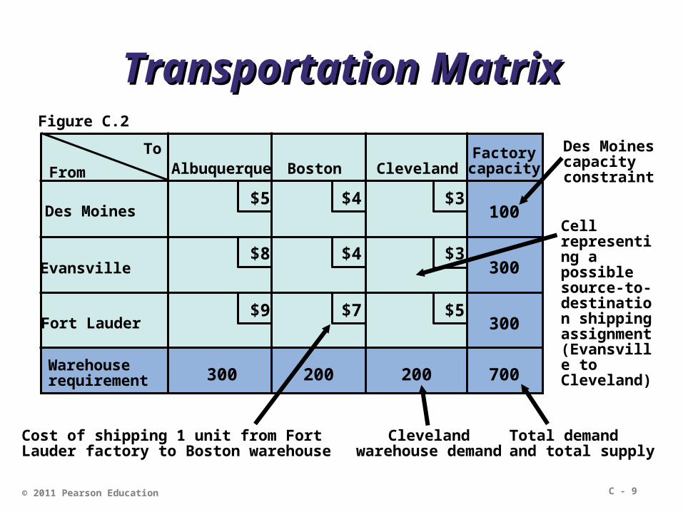
Transportation MatrixTransportation Matrix
From
ToAlbuquerque Boston Cleveland
Des Moines
Evansville
Fort Lauder
Factory capacity
Warehouse requirement
300
300
300 200 200
100
700
$5
$5
$4
$4
$3
$3
$9
$8
$7
Cost of shipping 1 unit from FortLauder factory to Boston warehouse
Des Moinescapacityconstraint
Cell representing a possible source-to-destination shipping assignment (Evansville to Cleveland)
Total demandand total supply
Clevelandwarehouse demand
Figure C.2

C - 10© 2011 Pearson Education
• Check the equality of the total supply & demand (if not, then we need for dummy solution )
• how many ship of unit should be transported from each demand to each distribution center can be expressed as (Xij)
• i ……..for demand and j …….for distribution center

C - 11
Step 2Step 2Establish the initial feasible Establish the initial feasible
solution solution
The Northwest corner rule
Least Cost Method
Vogel’s Approximation Model
© 2011 Pearson Education
C - 12© 2011 Pearson Education
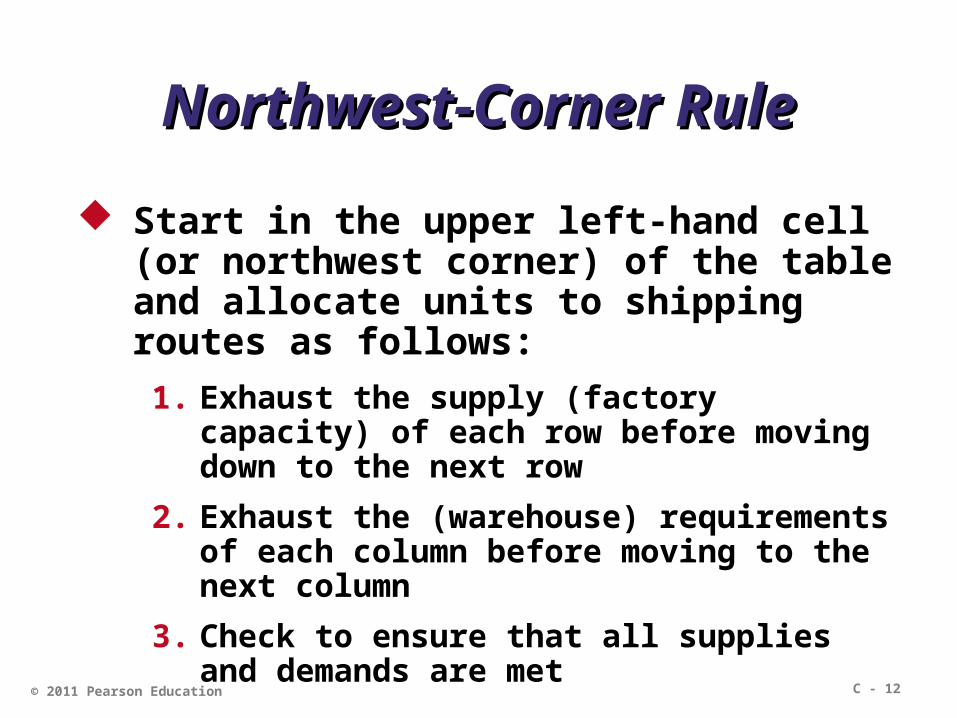
Northwest-Corner RuleNorthwest-Corner Rule
Start in the upper left-hand cell (or northwest corner) of the table and allocate units to shipping routes as follows:
1. Exhaust the supply (factory capacity) of each row before moving down to the next row
2. Exhaust the (warehouse) requirements of each column before moving to the next column
3. Check to ensure that all supplies and demands are met

C - 13
• The steps of the northwest corner method are summarized here:
• 1. Allocate as much as possible to the cell in the upper left-hand corner, subject to the supply and demand constraints.
• 2. Allocate as much as possible to the next adjacent feasible cell.
• 3. Repeat step 1,2 until all units all supply and demand have been satisfied
© 2011 Pearson Education

C - 14© 2011 Pearson Education
Northwest-Corner RuleNorthwest-Corner Rule
1. Assign 100 tubs from Des Moines to Albuquerque (exhausting Des Moines’s supply)
2. Assign 200 tubs from Evansville to Albuquerque (exhausting Albuquerque’s demand)
3. Assign 100 tubs from Evansville to Boston (exhausting Evansville’s supply)
4. Assign 100 tubs from Fort Lauder to Boston (exhausting Boston’s demand)
5. Assign 200 tubs from Fort Lauderdale to Cleveland (exhausting Cleveland’s demand and Fort Lauder’s supply)

C - 15© 2011 Pearson Education
To (A)Albuquerque
(B)Boston
(C)Cleveland
(D) Des Moines
(E) Evansville
(F) Fort Lauder
Warehouse requirement 300 200 200
Factory capacity
300
300
100
700
$5
$5
$4
$4
$3
$3
$9
$8
$7
From
Northwest-Corner RuleNorthwest-Corner Rule
100
100
100
200
200
Figure C.3
Means that the firm is shipping 100 bathtubs from Fort Lauder to Boston
C - 16© 2011 Pearson Education
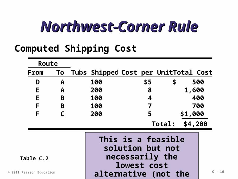
Northwest-Corner RuleNorthwest-Corner RuleComputed Shipping Cost
Table C.2
This is a feasible solution but not necessarily the
lowest cost alternative (not the optimal solution)
RouteFrom To Tubs Shipped Cost per Unit Total Cost
D A 100 $5 $ 500E A 200 8 1,600E B 100 4 400F B 100 7 700F C 200 5 $1,000
Total: $4,200

C - 17© 2011 Pearson Education
second Method second Method The Lowest-Cost Method The Lowest-Cost Method
1. Evaluate the transportation cost and select the square with the lowest cost (in case a Tie make an arbitrary selection )
2. Depending upon the supply & demand condition , allocate the maximum possible units to lowest cost square
3. Delete the satisfied allocated row or the column (or both)
4. Repeat steps 1 and 3 until all units have been allocated

C - 18© 2011 Pearson Education
The Lowest-Cost MethodThe Lowest-Cost MethodTo (A)
Albuquerque(B)
Boston(C)
Cleveland
(D) Des Moines
(E) Evansville
(F) Fort Lauder
Warehouse requirement 300 200 200
Factory capacity
300
300
100
700
$5
$5
$4
$4
$3
$3
$9
$8
$7
From
100
First, $3 is the lowest cost cell so ship 100 units from Des Moines to Cleveland and cross off the first row as Des Moines is satisfied
Figure C.4

C - 19© 2011 Pearson Education
The Lowest-Cost MethodThe Lowest-Cost MethodTo (A)
Albuquerque(B)
Boston(C)
Cleveland
(D) Des Moines
(E) Evansville
(F) Fort Lauderdale
Warehouse requirement 300 200 200
Factory capacity
300
300
100
700
$5
$5
$4
$4
$3
$3
$9
$8
$7
From
100
100
Second, $3 is again the lowest cost cell so ship 100 units from Evansville to Cleveland and cross off column C as Cleveland is satisfied
Figure C.4
C - 20© 2011 Pearson Education
The Lowest-Cost MethodThe Lowest-Cost MethodTo (A)
Albuquerque(B)
Boston(C)
Cleveland
(D) Des Moines
(E) Evansville
(F) Fort Lauderdale
Warehouse requirement 300 200 200
Factory capacity
300
300
100
700
$5
$5
$4
$4
$3
$3
$9
$8
$7
From
100
100
200
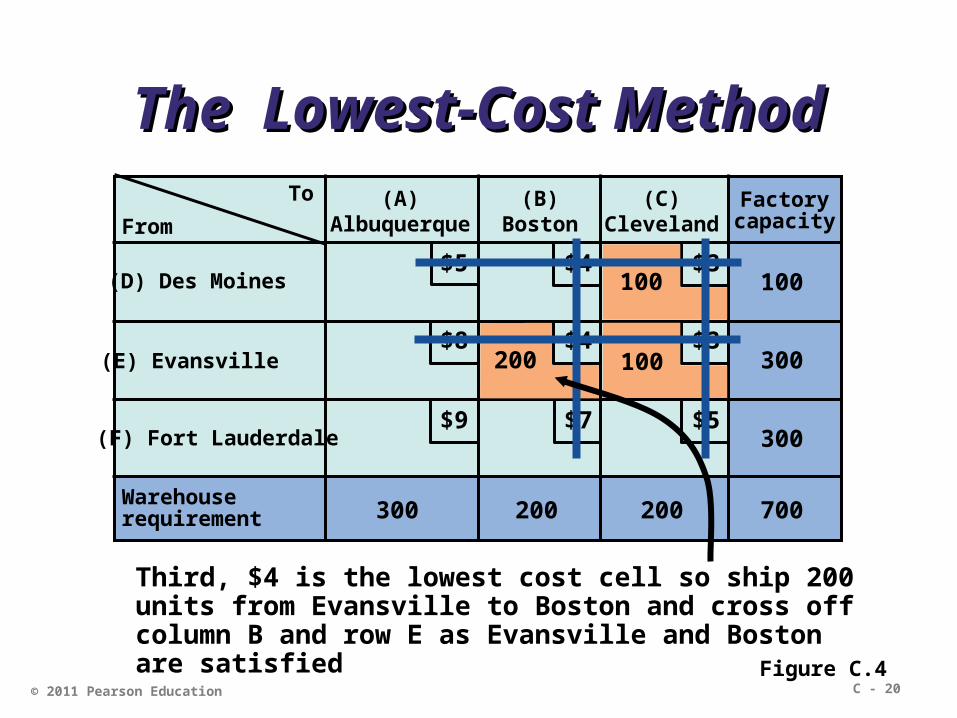
Third, $4 is the lowest cost cell so ship 200 units from Evansville to Boston and cross off column B and row E as Evansville and Boston are satisfied
Figure C.4
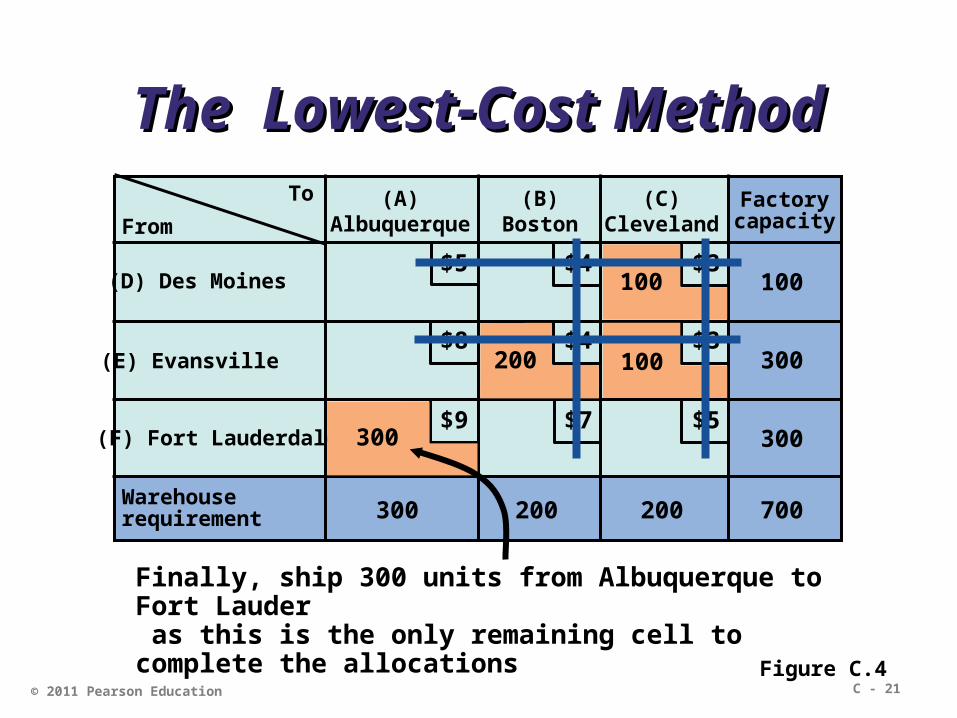
C - 21© 2011 Pearson Education
The Lowest-Cost MethodThe Lowest-Cost MethodTo (A)
Albuquerque(B)
Boston(C)
Cleveland
(D) Des Moines
(E) Evansville
(F) Fort Lauderdale
Warehouse requirement 300 200 200
Factory capacity
300
300
100
700
$5
$5
$4
$4
$3
$3
$9
$8
$7
From
100
100
200
300
Finally, ship 300 units from Albuquerque to Fort Lauder as this is the only remaining cell to complete the allocations
Figure C.4

C - 22© 2011 Pearson Education
The Lowest-Cost MethodThe Lowest-Cost MethodTo (A)
Albuquerque(B)
Boston(C)
Cleveland
(D) Des Moines
(E) Evansville
(F) Fort Lauderdale
Warehouse requirement 300 200 200
Factory capacity
300
300
100
700
$5
$5
$4
$4
$3
$3
$9
$8
$7
From
100
100
200
300
Total Cost = $3(100) + $3(100) + $4(200) + $9(300)= $4,100
Figure C.4

C - 23© 2011 Pearson Education
The Lowest-Cost MethodThe Lowest-Cost MethodTo (A)
Albuquerque(B)
Boston(C)
Cleveland
(D) Des Moines
(E) Evansville
(F) Fort Lauderdale
Warehouse requirement 300 200 200
Factory capacity
300
300
100
700
$5
$5
$4
$4
$3
$3
$9
$8
$7
From
100
100
200
300
Total Cost = $3(100) + $3(100) + $4(200) + $9(300)= $4,100
Figure C.4
This is a feasible solution, and an improvement over the previous solution, but not necessarily the lowest
cost alternative
C - 24© 2011 Pearson Education
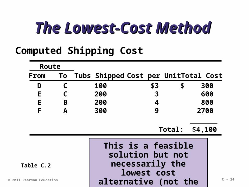
The Lowest-Cost Method The Lowest-Cost Method Computed Shipping Cost
Table C.2
This is a feasible solution but not necessarily the
lowest cost alternative (not the optimal solution)
RouteFrom To Tubs Shipped Cost per Unit Total Cost
D C 100 $3 $ 300E C 200 3 600E B 200 4 800F A 300 9 2700
Total: $4,100
C - 25
Testing the initial feasible Testing the initial feasible solution solution
• Test for optimality
• Optimal solution is achieved when there is no other alternative solution give lower cost.
• Two method for the optimal solution :-
• Stepping stone method
• Modified Distribution method (MODM)
© 2011 Pearson Education
C - 26© 2011 Pearson Education
Stepping-Stone MethodStepping-Stone Method
1. Proceed row by row and Select a water square (a square without any allocation) to evaluate
2. Beginning at this square, trace/forming a closed path back to the original square via squares that are currently being used
3. Beginning with a plus (+) sign at the unused corner (water square), place alternate minus and plus signs at each corner of the path just traced
C - 27© 2011 Pearson Education
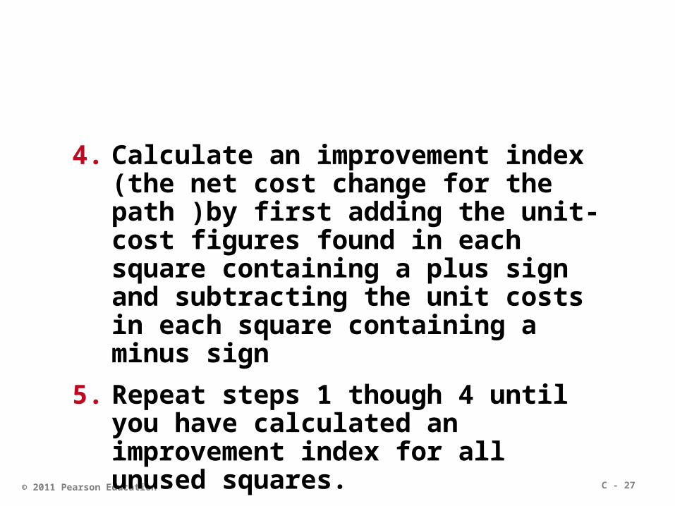
4. Calculate an improvement index (the net cost change for the path )by first adding the unit-cost figures found in each square containing a plus sign and subtracting the unit costs in each square containing a minus sign
5. Repeat steps 1 though 4 until you have calculated an improvement index for all unused squares.

C - 28
• Evaluate the solution from optimality test by observing the sign of the net cost change
I. The negative sign (-) indicates that a cost reduction can be made by making the change
II. Zero result indicates that there will be no change in cost
III. The positive sign (+) indicates an increase in cost if the change is made
IV. If all the signs are positive , it means that the optimal solution has been reached
V. If more than one squares have a negative signs then the water squared with the largest negative net cost change is selected for quicker solution , in case of tie; choose one of them randomly
© 2011 Pearson Education

C - 29© 2011 Pearson Education
6. If an improvement is possible, choose the route (unused square) with the largest negative improvement index
7. On the closed path for that route, select the smallest number found in the squares containing minus signs, adding this number to all squares on the closed path with plus signs and subtract it from all squares with a minus sign .Repeat these process until you have evaluate all unused squares
8. Prepare the new transportation table and check for the optimality
C - 30© 2011 Pearson Education
$5
$8 $4
$4
+ -
+-
Stepping-Stone MethodStepping-Stone MethodTo (A)
Albuquerque(B)
Boston(C)
Cleveland
(D) Des Moines
(E) Evansville
(F) Fort Lauderdale
Warehouse requirement 300 200 200
Factory capacity
300
300
100
700
$5
$5
$4
$4
$3
$3
$9
$8
$7
From
100
100
100
200
200
+-
-+
1100
201 99
99
100200Figure C.5
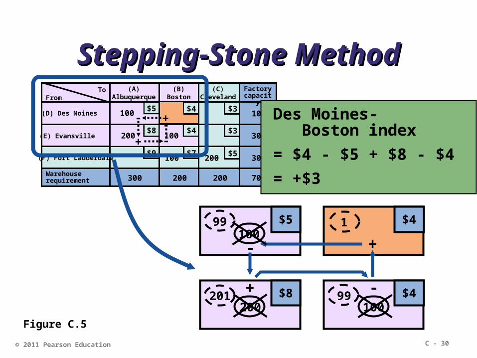
Des Moines- Boston index
= $4 - $5 + $8 - $4
= +$3

C - 31© 2011 Pearson Education
Stepping-Stone MethodStepping-Stone MethodTo (A)
Albuquerque(B)
Boston(C)
Cleveland
(D) Des Moines
(E) Evansville
(F) Fort Lauder
Warehouse requirement 300 200 200
Factory capacity
300
300
100
700
$5
$5
$4
$4
$3
$3
$9
$8
$7
From
100
100
100
200
200
Figure C.6
Start
+-
+
-+
-
Des Moines-Cleveland index
= $3 - $5 + $8 - $4 + $7 - $5 = +$4

C - 32© 2011 Pearson Education
Stepping-Stone MethodStepping-Stone MethodTo (A)
Albuquerque(B)
Boston(C)
Cleveland
(D) Des Moines
(E) Evansville
(F) Fort Lauderdale
Warehouse requirement 300 200 200
Factory capacity
300
300
100
700
$5
$5
$4
$4
$3
$3
$9
$8
$7
From
100
100
100
200
200
Evansville-Cleveland index
= $3 - $4 + $7 - $5 = +$1
(Closed path = EC - EB + FB - FC)
Fort Lauder-Albuquerque index
= $9 - $7 + $4 - $8 = -$2
(Closed path = FA - FB + EB - EA)

C - 33© 2011 Pearson Education
Stepping-Stone MethodStepping-Stone MethodTo (A)
Albuquerque(B)
Boston(C)
Cleveland
(D) Des Moines
(E) Evansville
(F) Fort Lauder
Warehouse requirement 300 200 200
Factory capacity
300
300
100
700
$5
$5
$4
$4
$3
$3
$9
$8
$7
From
100
100
100
200
200
Figure C.7
+
+-
-
1. Add 100 units on route FA2. Subtract 100 from routes FB3. Add 100 to route EB4. Subtract 100 from route EA

C - 34© 2011 Pearson Education
The first modified transportation table The first modified transportation table by Stepping-Stone Methodby Stepping-Stone Method
To (A)Albuquerque
(B)Boston
(C)Cleveland
(D) Des Moines
(E) Evansville
(F) Fort Lauderdale
Warehouse requirement 300 200 200
Factory capacity
300
300
100
700
$5
$5
$4
$4
$3
$3
$9
$8
$7
From
100
200
100
100
200
Figure C.8
Total Cost = $5(100) + $8(100) + $4(200) + $9(100) + $5(200)= $4,000 is this the optimal solution

C - 35
• Since the condition for the acceptability is met (m+n -1 = the used cells )
• Repeat steps 1 though 4 until you have calculated an improvement index for all unused squares.
• Evaluate the unused cells as follow ;
•
© 2011 Pearson Education
C - 36
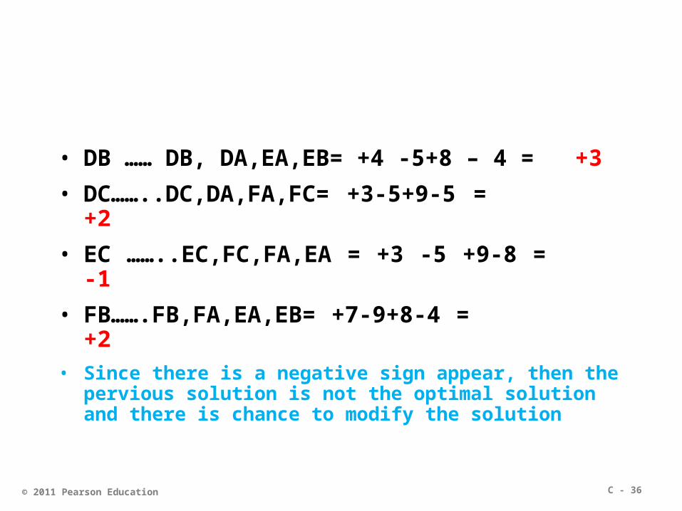
• DB …… DB, DA,EA,EB= +4 -5+8 – 4 = +3
• DC……..DC,DA,FA,FC= +3-5+9-5 = +2
• EC ……..EC,FC,FA,EA = +3 -5 +9-8 = -1
• FB…….FB,FA,EA,EB= +7-9+8-4 = +2
• Since there is a negative sign appear, then the pervious solution is not the optimal solution and there is chance to modify the solution
© 2011 Pearson Education
C - 37© 2011 Pearson Education
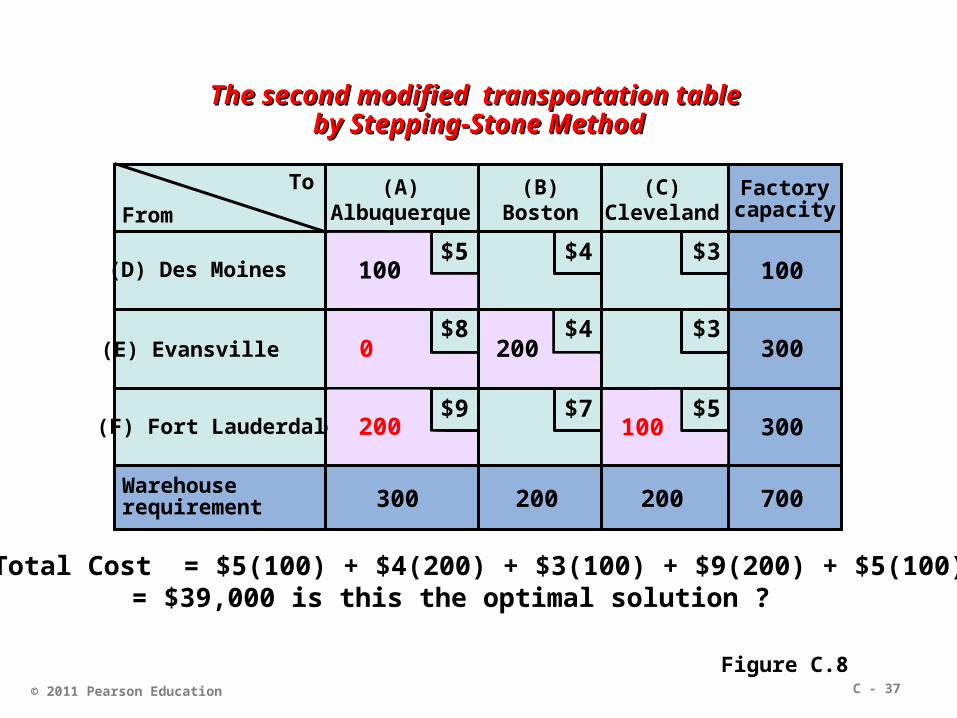
The second modified transportation table The second modified transportation table by Stepping-Stone Methodby Stepping-Stone Method
100
To (A)Albuquerque
(B)Boston
(C)Cleveland
(D) Des Moines
(E) Evansville
(F) Fort Lauderdale
Warehouse requirement 300 200 200
Factory capacity
300
300
100
700
$5
$5
$4
$4
$3
$3
$9
$8
$7
From
200
200
100
0
100
Figure C.8
Total Cost = $5(100) + $4(200) + $3(100) + $9(200) + $5(100)= $39,000 is this the optimal solution ?

C - 38
Re-evaluate the unused Re-evaluate the unused cells cells
• AD; DB,EB,EC,FC,FA,AD= +4-4+3-5+9-5 = +2
• DC; DC,FC,FA,DA= +3 -5+9-5 = +2
• EA; EA,EC,FC,FA =+8 -3+5-9 = +1
• FB; FB,EB,EC,FC= +7 – 4 +3 – 5 = +1
• Since there is no negative sign appear, then the pervious solution is the optimal solution and there is no chance to modify the solution
© 2011 Pearson Education

C - 39
• The initial cost = $4,200
• The first modified cost = $4,000
• The second modified cost= $39,000
• Optimal solution
© 2011 Pearson Education

C - 40© 2011 Pearson Education
Special Issues in ModelingSpecial Issues in Modeling
Demand not equal to supply Called an unbalanced problem
Common situation in the real world
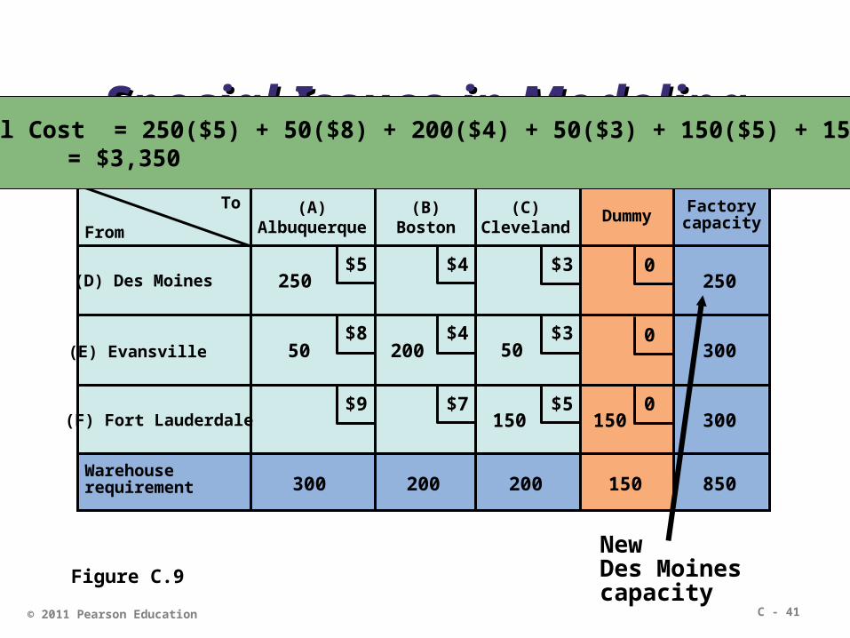
Resolved by introducing dummy sources or dummy destinations as necessary with cost coefficients of zero
C - 41© 2011 Pearson Education
Special Issues in ModelingSpecial Issues in Modeling
Figure C.9
NewDes Moines capacity
To (A)Albuquerque
(B)Boston
(C)Cleveland
(D) Des Moines
(E) Evansville
(F) Fort Lauderdale
Warehouse requirement 300 200 200
Factory capacity
300
300
250
850
$5
$5
$4
$4
$3
$3
$9
$8
$7
From
50200
250
50
150
Dummy
150
0
0
0
150
Total Cost = 250($5) + 50($8) + 200($4) + 50($3) + 150($5) + 150(0)= $3,350
C - 42© 2011 Pearson Education
Special Issues in ModelingSpecial Issues in Modeling
DegeneracyWe must make the test for acceptability to use the stepping-stone
methodology, that mean the feasible solution must met the condition of the number of occupied squares in any solution must be equal to the number of rows in the table plus the number of columns minus 1
M (number of rows) + N (number of columns ) = allocated cells
If a solution does not satisfy this rule it is called degenerate
C - 43© 2011 Pearson Education
To Customer1
Customer2
Customer3
Warehouse 1
Warehouse 2
Warehouse 3
Customer demand 100 100 100
Warehouse supply
120
80
100
300
$8
$7
$2
$9
$6
$9
$7
$10
$10
From
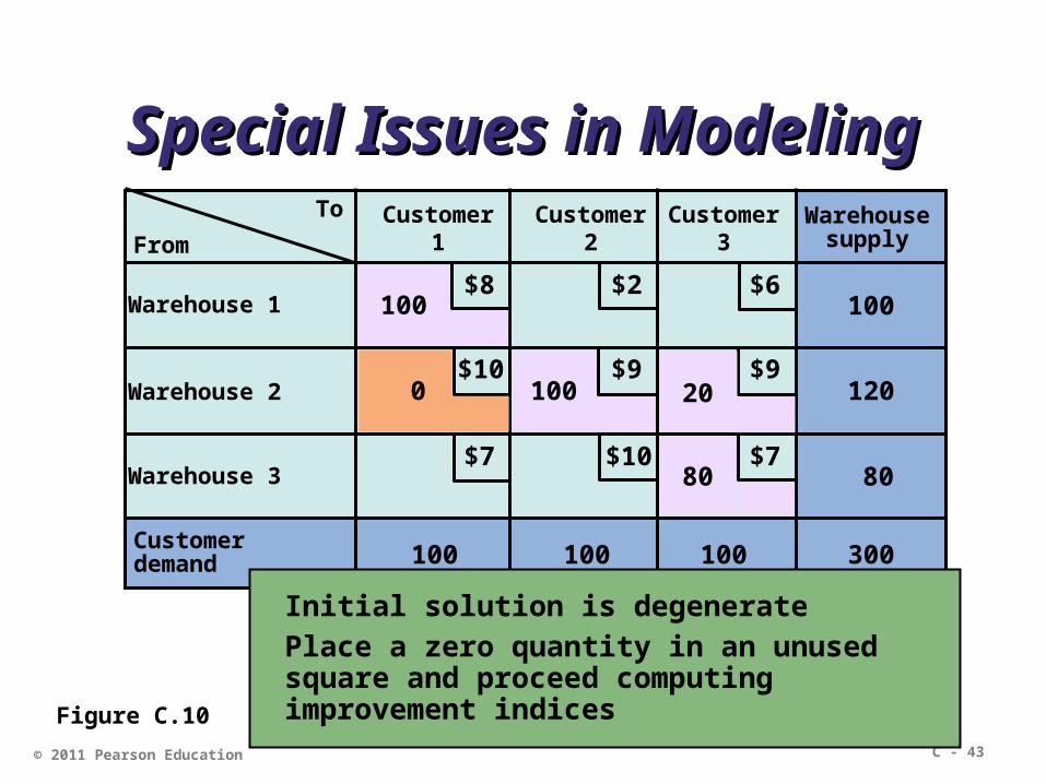
Special Issues in ModelingSpecial Issues in Modeling
0 100
100
80
20
Figure C.10
Initial solution is degeneratePlace a zero quantity in an unused square and proceed computing improvement indices

C - 44© 2011 Pearson Education
All rights reserved. No part of this publication may be reproduced, stored in a retrieval system, or transmitted, in any form or by any means, electronic, mechanical, photocopying,
recording, or otherwise, without the prior written permission of the publisher. Printed in the United States of America.