c 2007 by ganesh bikshandi. all rights . · pdf filespecial thanks to basilio. b. ......
TRANSCRIPT

c© 2007 by Ganesh Bikshandi. All rights reserved.
PARALLEL PROGRAMMING WITH HIERARCHICALLY TILED ARRAYS
BY
GANESH BIKSHANDI
B.E., University of Madras, 2000
DISSERTATION
Submitted in partial fulfillment of the requirementsfor the degree of Doctor of Philosophy in Computer Science
in the Graduate College of theUniversity of Illinois at Urbana-Champaign, 2007
Urbana, Illinois

To my family.
iii
Acknowledgments
This project would not have been possible without the support of many people. Many thanks
to my adviser, David A. Padua, who read my numerous revisions and helped make some
sense of the confusion. Also thanks to my committee members, Vikram Adve, Laxmikant
Kale, Micheal Heath, Maria Jesus Garzaran and Christoph von Praun who offered guidance
and support.
Special thanks to Basilio. B. Fraguela, for his advice on several technical issues relating to
the topic of this dissertation, Jia Guo, my research partner, David Kuck (Intel), upon whose
guidance I entered the graduate school of UIUC, Gheorghe Almasi and Calin Cascaval, for
their support in continuing this work at the IBM T. J. Watson research center.
I am deeply indebted to my father, mother, two brothers (Balaji & Barani), sister-in-
law (Tamizharasi), aunt (Mallika) and to everyone else in my family, who helped me reach
the pinnacle of education from an humble background in India. An extra thanks to my
elder brother Balaji, the whizkid of our family, who introduced me to the computers and
internet. Finally, thanks to my roommates (Kalyan Babu, Sahail) and neighbors (Sri Krishna
Marathe), who endured their stay with me for five long years.
iv
Abstract
Writing high performance programs is a non-trivial task and remains a challenge even to
advanced programmers. This dissertation describes a new data type, Hierarchically Tiled
Array (HTA), that simplifies this task. HTAs are tiled arrays whose elements can either be
HTAs or arrays or scalars. The elements can be distributed among a cluster of computers
or be collocated in a single processor. They can be accessed and operated like scalars of the
conventional n-dimensional arrays. They can also be assigned to one another, or passed as
arguments to a function. In essence, HTA is an attempt to adopt tiles as first class data
types, and to allow their direct manipulation.
Augmenting existing programming languages with HTAs offers several benefits to high
performance program developers. HTAs provide a global shared memory abstraction; this
significantly reduces the time to develop parallel programs. The control flow of parallel HTA
programs resemble sequential programs and hence are very easy to reason. HTAs naturally
facilitate the development of recursive blocked algorithms aimed at exploiting deep memory
hierarchies. The rich set of well defined operations and vector style expressions lead to code
with high clarity and smaller size. Since HTAs are also conventional arrays, their fusion with
a language will not add extra burden to programmers. Moreover, the performance benefits
of tiling are preserved.
To prove these claims, two popular languages, C++ and MATLAB, have been extended
with HTA. In addition, the NAS benchmark suite, a set of complex computation intensive
parallel programs, have been re-written using HTAs. We compare the lines of code and
execution times of HTA programs with that of FORTRAN versions. Our results show
v

that the codes written using HTAs are very readable and at the same efficient. We also
show several sample code snippets to demonstrate the clarity of the HTA programs. All
the experiments indicate that the explicit notion of tiles makes HTA a powerful language
construct for writing a wide range of high performance programs.
vi
Table of Contents
List of Tables . . . . . . . . . . . . . . . . . . . . . . . . . . . . . . . . . . . . ix
List of Figures . . . . . . . . . . . . . . . . . . . . . . . . . . . . . . . . . . . . x
Chapter 1 Introduction . . . . . . . . . . . . . . . . . . . . . . . . . . . . . 11.1 Overview . . . . . . . . . . . . . . . . . . . . . . . . . . . . . . . . . . . . . . 11.2 Contributions of this thesis . . . . . . . . . . . . . . . . . . . . . . . . . . . . 41.3 Thesis Organization . . . . . . . . . . . . . . . . . . . . . . . . . . . . . . . . 6
Chapter 2 Hierarchically Tiled Arrays and Operations . . . . . . . . . . . 72.1 Hierarchically Tiled Arrays . . . . . . . . . . . . . . . . . . . . . . . . . . . . 7
2.1.1 Classification . . . . . . . . . . . . . . . . . . . . . . . . . . . . . . . 72.1.2 Symbols, Notations and Terminologies . . . . . . . . . . . . . . . . . 102.1.3 Construction of HTAs . . . . . . . . . . . . . . . . . . . . . . . . . . 13
2.2 HTA Operations . . . . . . . . . . . . . . . . . . . . . . . . . . . . . . . . . 152.2.1 Query Operations . . . . . . . . . . . . . . . . . . . . . . . . . . . . . 162.2.2 Element Access operations . . . . . . . . . . . . . . . . . . . . . . . . 162.2.3 Point-wise operations . . . . . . . . . . . . . . . . . . . . . . . . . . . 182.2.4 Collective Operations . . . . . . . . . . . . . . . . . . . . . . . . . . . 252.2.5 Higher-order Operators . . . . . . . . . . . . . . . . . . . . . . . . . . 302.2.6 Composing of operations . . . . . . . . . . . . . . . . . . . . . . . . . 35
2.3 Parallel Semantics of HTA operations . . . . . . . . . . . . . . . . . . . . . . 362.3.1 Distributed HTA construction . . . . . . . . . . . . . . . . . . . . . . 362.3.2 Unary Operations . . . . . . . . . . . . . . . . . . . . . . . . . . . . . 372.3.3 Binary Operations . . . . . . . . . . . . . . . . . . . . . . . . . . . . 372.3.4 HTA access operation . . . . . . . . . . . . . . . . . . . . . . . . . . 392.3.5 Assignments . . . . . . . . . . . . . . . . . . . . . . . . . . . . . . . . 402.3.6 Map . . . . . . . . . . . . . . . . . . . . . . . . . . . . . . . . . . . . 412.3.7 Reduce . . . . . . . . . . . . . . . . . . . . . . . . . . . . . . . . . . . 412.3.8 Collective operations . . . . . . . . . . . . . . . . . . . . . . . . . . . 42
Chapter 3 Implementation . . . . . . . . . . . . . . . . . . . . . . . . . . . 463.1 Introduction . . . . . . . . . . . . . . . . . . . . . . . . . . . . . . . . . . . . 463.2 Execution Model of HTA programs . . . . . . . . . . . . . . . . . . . . . . . 473.3 Underlying Implementation . . . . . . . . . . . . . . . . . . . . . . . . . . . 493.4 MATLAB Library . . . . . . . . . . . . . . . . . . . . . . . . . . . . . . . . . 52
vii

3.4.1 The HTA class data type . . . . . . . . . . . . . . . . . . . . . . . . . 523.4.2 Interfacing with MPI and Other implementation details . . . . . . . . 533.4.3 Run time overheads . . . . . . . . . . . . . . . . . . . . . . . . . . . . 54
3.5 C++ . . . . . . . . . . . . . . . . . . . . . . . . . . . . . . . . . . . . . . . . 553.5.1 Overview . . . . . . . . . . . . . . . . . . . . . . . . . . . . . . . . . 553.5.2 Front End classes . . . . . . . . . . . . . . . . . . . . . . . . . . . . . 553.5.3 Back End classes . . . . . . . . . . . . . . . . . . . . . . . . . . . . . 563.5.4 Performance Optimizations . . . . . . . . . . . . . . . . . . . . . . . 58
3.6 Examples . . . . . . . . . . . . . . . . . . . . . . . . . . . . . . . . . . . . . 593.6.1 Matrix Multiplication . . . . . . . . . . . . . . . . . . . . . . . . . . . 593.6.2 Iterative Jacobi Solver . . . . . . . . . . . . . . . . . . . . . . . . . . 64
Chapter 4 Evaluation . . . . . . . . . . . . . . . . . . . . . . . . . . . . . . . 674.1 Introduction . . . . . . . . . . . . . . . . . . . . . . . . . . . . . . . . . . . . 674.2 Description of the NAS benchmark programs . . . . . . . . . . . . . . . . . . 69
4.2.1 EP . . . . . . . . . . . . . . . . . . . . . . . . . . . . . . . . . . . . . 694.2.2 MG . . . . . . . . . . . . . . . . . . . . . . . . . . . . . . . . . . . . . 734.2.3 CG . . . . . . . . . . . . . . . . . . . . . . . . . . . . . . . . . . . . . 794.2.4 FT . . . . . . . . . . . . . . . . . . . . . . . . . . . . . . . . . . . . . 834.2.5 IS . . . . . . . . . . . . . . . . . . . . . . . . . . . . . . . . . . . . . 864.2.6 BT . . . . . . . . . . . . . . . . . . . . . . . . . . . . . . . . . . . . . 894.2.7 LU . . . . . . . . . . . . . . . . . . . . . . . . . . . . . . . . . . . . . 94
4.3 Experimental Results . . . . . . . . . . . . . . . . . . . . . . . . . . . . . . . 974.3.1 MATLAB Library . . . . . . . . . . . . . . . . . . . . . . . . . . . . 1004.3.2 C++ Library . . . . . . . . . . . . . . . . . . . . . . . . . . . . . . . 1064.3.3 Summary . . . . . . . . . . . . . . . . . . . . . . . . . . . . . . . . . 114
4.4 SLOC measurement . . . . . . . . . . . . . . . . . . . . . . . . . . . . . . . . 116
Chapter 5 Related Works . . . . . . . . . . . . . . . . . . . . . . . . . . . . 1195.1 Introduction . . . . . . . . . . . . . . . . . . . . . . . . . . . . . . . . . . . . 1195.2 APL . . . . . . . . . . . . . . . . . . . . . . . . . . . . . . . . . . . . . . . . 1225.3 HPF . . . . . . . . . . . . . . . . . . . . . . . . . . . . . . . . . . . . . . . . 1245.4 ZPL . . . . . . . . . . . . . . . . . . . . . . . . . . . . . . . . . . . . . . . . 1275.5 POOMA . . . . . . . . . . . . . . . . . . . . . . . . . . . . . . . . . . . . . . 1305.6 Split-C . . . . . . . . . . . . . . . . . . . . . . . . . . . . . . . . . . . . . . . 1325.7 Sequoia . . . . . . . . . . . . . . . . . . . . . . . . . . . . . . . . . . . . . . 1345.8 Summary . . . . . . . . . . . . . . . . . . . . . . . . . . . . . . . . . . . . . 135
Chapter 6 Conclusions . . . . . . . . . . . . . . . . . . . . . . . . . . . . . . 1416.1 Conclusions . . . . . . . . . . . . . . . . . . . . . . . . . . . . . . . . . . . . 1416.2 Future Work . . . . . . . . . . . . . . . . . . . . . . . . . . . . . . . . . . . . 142
6.2.1 Implementation of new language constructs . . . . . . . . . . . . . . 1426.2.2 Improving the syntax of HTA programs . . . . . . . . . . . . . . . . . 1436.2.3 Improving the performance of HTA programs . . . . . . . . . . . . . 143
References . . . . . . . . . . . . . . . . . . . . . . . . . . . . . . . . . . . . . . 149
Author’s Biography . . . . . . . . . . . . . . . . . . . . . . . . . . . . . . . . . 153
viii

List of Tables
2.1 Summary of HTA operations. . . . . . . . . . . . . . . . . . . . . . . . . . . . . . . . 36
3.1 MATLAB and C++ syntax for various HTA operations. . . . . . . . . . . . . . . . . . . . . 473.2 HTA operations and the corresponding MPI communication primitives used. . . . . . . . . . . . . 51
4.1 Characteristics of Computation and Communication of the programs of NAS benchmark set. . . . . . 674.2 Correspondence between Array and HTA operations. . . . . . . . . . . . . . . . . . . . . . 684.3 Data types and various input sizes of the benchmark programs . . . . . . . . . . . . . . . . . 974.4 Configuration of the experimental environments. . . . . . . . . . . . . . . . . . . . . . . . 984.5 Tiling structure and processor distribution. . . . . . . . . . . . . . . . . . . . . . . . . . 984.6 Execution times in seconds for some of the applications in the NAS benchmarks for F77+MPI versus MAT-
LAB+HTA. The execution time for 1 processor corresponds to the serial application in F77 or MATLAB,
without MPI or HTAs. The execution environment is the Tungsten cluster. . . . . . . . . . . . . 1014.7 Ratio of execution times (MATLAB+HTA
F77+MPI). The execution environment is the tungsten cluster. . . . . 102
4.8 Execution times in seconds for programs in the NAS benchmarks for F77+MPI and CPP+HTA. The
execution environment is the turing cluster. Input size for LU is CLASS A. For all others, it is class C. . 1054.9 Ratio of execution times (CPP+HTA
F77+MPI). The execution environment is the turing cluster. Input size for
LU is CLASS A. For all others, it is class C. . . . . . . . . . . . . . . . . . . . . . . . . . 1064.10 Comparison of running times (seconds) of pure-HTA and map versions of MG (CLASS C) in turing cluster. 108
5.1 Characterization of parallel programming infrastructures. . . . . . . . . . . . . . . . . . . . . 136
ix

List of Figures
2.1 Homogeneous Hierarchically Tiled Array (a) Regular (b) Irregular . . . . . . 82.2 An Illegal HTA . . . . . . . . . . . . . . . . . . . . . . . . . . . . . . . . . . 82.3 A Two level HTA . . . . . . . . . . . . . . . . . . . . . . . . . . . . . . . . . 92.4 Heterogeneous HTAs with (a) different position of the partition for adjacent
tiles (b) different levels of tiling . . . . . . . . . . . . . . . . . . . . . . . . . 92.5 Naming and Numbering conventions of the various levels of an HTA . . . . . 102.6 Illustration of (a) tuple, range, region and (b) dist . . . . . . . . . . . . . 122.7 Bottom Construction of HTAs . . . . . . . . . . . . . . . . . . . . . . . . . . 132.8 Top–down HTA construction (a MATLAB like pseudo-code) . . . . . . . . . 142.9 HTA Accessing Operation . . . . . . . . . . . . . . . . . . . . . . . . . . . . 162.10 Logical Indexing of HTAs . . . . . . . . . . . . . . . . . . . . . . . . . . . . 182.11 The need for conformability a) Ambiguity in HTA operations b) Illegal HTA
operations . . . . . . . . . . . . . . . . . . . . . . . . . . . . . . . . . . . . . 202.12 An illustration of the HTA rules of operation . . . . . . . . . . . . . . . . . . 222.13 HTA Assignments . . . . . . . . . . . . . . . . . . . . . . . . . . . . . . . . . 252.14 HTA transpose operation a) with tlevel = 0 on an HTA of height 1 b) with
tlevel =1 on an HTA of height 2. . . . . . . . . . . . . . . . . . . . . . . . . 262.15 Swapping the tiles in 2 successive hierarchies using htranspose . . . . . . . 282.16 (a) HTA Permutation (b) circshift using Permutation . . . . . . . . . . . 282.17 Replication of Tiles of an HTA using repmat . . . . . . . . . . . . . . . . . . 292.18 HTA map operator . . . . . . . . . . . . . . . . . . . . . . . . . . . . . . . . 312.19 HTA reduce operator . . . . . . . . . . . . . . . . . . . . . . . . . . . . . . 322.20 HTA scan operator . . . . . . . . . . . . . . . . . . . . . . . . . . . . . . . . 352.21 HTA reduce operator combined with map . . . . . . . . . . . . . . . . . . . 352.22 HTA scan operator combined with map . . . . . . . . . . . . . . . . . . . . . 352.23 Communication in a parallel binary operation a) HTAs of same shape b)
HTAs of different shape. The mapping of the operand HTAs is shown in thefigures using processor number in each tile. . . . . . . . . . . . . . . . . . . . 38
2.24 A chain of binary expression with HTAs of different processor mapping . . . 392.25 Projection of an 2-D (left hand side) array along dimension = 1 . . . . . . . 412.26 Communication in a partial reduce operation along dim=1, without repli-
cation. The left hand side sub-figures describes the distribution of input HTA,the right hand side sub-figure describes the distribution of output HTA . . . 42
x
2.27 Communication in a transpose operation a) square HTA b) non-square HTA.In both the figures, the left hand side sub-figures describe the distribution ofinput HTA, the right hand side sub-figures describe the distribution of theoutput HTA. In (b) the middle figure is the transposed distribution of theinput HTA . . . . . . . . . . . . . . . . . . . . . . . . . . . . . . . . . . . . . 43
2.28 Communication in a repmat operation. In the figure, the left hand side sub-figure describes the distribution of input HTA, the right hand side sub-figuredescribes the distribution of output HTA. . . . . . . . . . . . . . . . . . . . . 44
3.1 Simple code example . . . . . . . . . . . . . . . . . . . . . . . . . . . . . . . 483.2 (a) Example of code with concurrent execution. (b) Timeline for the proces-
sors executing the code in (a). . . . . . . . . . . . . . . . . . . . . . . . . . . 493.3 HTA implementation. . . . . . . . . . . . . . . . . . . . . . . . . . . . . . . . 503.4 Hierarchy of the Back End classes . . . . . . . . . . . . . . . . . . . . . . . . 573.5 Relaxing sequential evaluation order to facilitate overlap of communication
and computation. . . . . . . . . . . . . . . . . . . . . . . . . . . . . . . . . . 583.6 Recursive matrix-matrix multiplication that exploits cache locality. . . . . . 603.7 HTA version of SUMMA Algorithm . . . . . . . . . . . . . . . . . . . . . . . 623.8 The communication steps in Cannon’s algorithm on 16 processors . . . . . . 633.9 Cannon’s algorithm using HTAs. . . . . . . . . . . . . . . . . . . . . . . . . 633.10 Jacobi computation using HTA . . . . . . . . . . . . . . . . . . . . . . . . . 643.11 Graphical Illustration of Jacobi computation (a) Communication of boundary
regions (b) Stencil computation . . . . . . . . . . . . . . . . . . . . . . . . . 65
4.1 (a) Illustration of the EP algorithm. (b) Sequence splitting algorithm forgeneration random numbers in parallel . . . . . . . . . . . . . . . . . . . . . 70
4.2 NAS EP benchmark using HTA (a) MATLAB-serial (b) MALAB-HTA . . . 724.3 NAS EP Benchmark written using map construct and HTAs . . . . . . . . . 734.4 Illustration of (a) interpolation and (b) projection. For simplicity, a 1D
grid is shown here . . . . . . . . . . . . . . . . . . . . . . . . . . . . . . . . . 744.5 Pictorial view of HTA projection . . . . . . . . . . . . . . . . . . . . . . . 754.6 The main procedure of MG in MATLAB . . . . . . . . . . . . . . . . . . . . . 754.7 MG resid (a) MATLAB-serial version (b) MATLAB+HTA version . . . . . . 764.8 MG psinv (a) MATLAB-serial version (b) MATLAB+HTA version . . . . . . 764.9 MG rprj3 (a) MATLAB-serial version (b) MATLAB+HTA version . . . . . . 774.10 MG interp (a) MATLAB-serial version (b) MATLAB+HTA version . . . . . 784.11 MG comm3 a) MATLAB-serial b) MATLAB+HTA version . . . . . . . . . . . 794.12 Assignment using HTAs (a) along the direction of west (b) along the direction
of south . . . . . . . . . . . . . . . . . . . . . . . . . . . . . . . . . . . . . . 794.13 Graphical Illustration of the steps in the CG benchmark . . . . . . . . . . . . 804.14 CG Benchmark (a) MATLAB-serial implementation (b) MATLAB+HTA im-
plementation . . . . . . . . . . . . . . . . . . . . . . . . . . . . . . . . . . . 824.15 FT Benchmark (a) HTA-serial version (b) MATLAB+HTA version . . . . . 834.16 Illustration of the FT benchmark program . . . . . . . . . . . . . . . . . . . . 854.17 IS Benchmark (a) C-serial version (b) CPP-HTA version . . . . . . . . . . . 874.18 Illustration of the IS benchmark (HTA version) . . . . . . . . . . . . . . . . 88
xi
4.19 (a) Flow of control in BT (b) Double cyclic mapping for optimal performance 924.20 x-sweep section of BT (a) MATLAB-serial version (b) MATLAB+HTA version 934.21 Hyperplane . . . . . . . . . . . . . . . . . . . . . . . . . . . . . . . . . . . . 954.22 Forward phase of a simple SSOR iteration a) Using MATLAB serial program
b) Using MATLAB HTA program c) Illustration of the diagonal iteration overthe tiles . . . . . . . . . . . . . . . . . . . . . . . . . . . . . . . . . . . . . . 96
4.23 Running time comparison of F77+MPI and CPP+HTA on Turing cluster :EP Benchmark (Class C) . . . . . . . . . . . . . . . . . . . . . . . . . . . . . 106
4.24 Running time comparison of F77+MPI and CPP+HTA on Turing cluster:MG Benchmark (Class C) . . . . . . . . . . . . . . . . . . . . . . . . . . . . 107
4.25 Running time comparison of F77+MPI and CPP+HTA on Turing cluster:CG Benchmark (Class C) . . . . . . . . . . . . . . . . . . . . . . . . . . . . 109
4.26 Running time comparison of F77+MPI and CPP+HTA on Turing Cluster :FT Benchmark (Class C) . . . . . . . . . . . . . . . . . . . . . . . . . . . . . 110
4.27 Running time comparison of C+MPI and CPP+HTA on Turing cluster: ISBenchmark (Class C) . . . . . . . . . . . . . . . . . . . . . . . . . . . . . . . 112
4.28 Running time comparison of F77+MPI and CPP+HTA on Turing cluster:LU Benchmark (Class A) . . . . . . . . . . . . . . . . . . . . . . . . . . . . . 113
4.29 Linecount of key sections of MATLAB+HTA, CPP+HTA and F77+ MPIprograms. . . . . . . . . . . . . . . . . . . . . . . . . . . . . . . . . . . . . . 116
5.1 1-D Jacobi Relaxation a) Serial FORTRAN program b) MPI Program . . . . 1205.2 Representing a relational data base system in APL2 using arrays of arrays. . 1235.3 HPF version of the 1-D Jacobi computation . . . . . . . . . . . . . . . . . . 1255.4 ZPL version of the 1-D Jacobi computation . . . . . . . . . . . . . . . . . . . 1275.5 POOMA version of the 1-D Jacobi computation . . . . . . . . . . . . . . . . 1305.6 Split-C version of a 1-D Jacobi-like computation . . . . . . . . . . . . . . . . 1335.7 A declaration for a blocked/cyclic layout in both dimensions. Each block
shows the number of the processor that owns it. Shown for n=8, m=9, r=4,c=3, where there are 12 processors. The Figure is reproduced from [23]. . . . 134
1 FORTRAN+MPI implementation of the CG benchmark . . . . . . . . . . . 1452 Transpositions in FT benchmark in FORTRAN+MPI version : x yz and xy z
transpositioon . . . . . . . . . . . . . . . . . . . . . . . . . . . . . . . . . . . 1463 Transpositions in FT benchmark in FORTRAN+MPI version (a) x z trans-
position (b) x y transposition . . . . . . . . . . . . . . . . . . . . . . . . . . 1474 FORTRAN+MPI implementation of the IS benchmark . . . . . . . . . . . . 148
xii
Chapter 1
Introduction
1.1 Overview
Parallel computing has long been perceived as the solution to meet the demands of compu-
tational power and memory requirements. A typical strategy to improve performance is to
combine several computers or processors which co-operate with each other in the execution of
programs. This approach reduces the time to completion of tasks by increasing both compu-
tational power and main memory size. Traditionally, the need for writing parallel programs
was mostly faced by scientists and engineers at academic and research institutions; a parallel
computer is costly to be used for commodity applications, and only scientific computations
demand huge memory and computational power, justifying the use of parallel computers.
Over the past few years, the domain of parallel processing is shifting to modern fields like
data mining and web crawling. Additionally, it has become easy to convert a cluster of PCs
in to a powerful parallel computer easily using adequate software support. Large companies
like Google execute several compute-intensive tasks in such clusters [24]. Furthermore, with
the ubiquity of multi-core multiprocessors and the emergence of new architectures like cell
processors [44] , parallel programming is becoming commonplace. Soon, the main stream
computing industries will face the task of writing clean and efficient parallel programs either
for their in-house tasks or for commercial softwares.
Parallel programming is a challenging task. Unlike a sequential program, a parallel
program is executed by P processors; this imposes extra responsibility on a programmer
to utilize them efficiently. Roughly, the programmer has to write extra code to perform
1

the following tasks: decomposition of the problem domain in to P sub-domains, identifying
P sub-tasks to operate on these domains, and synchronizing the sub-tasks. Though these
appear to be conceptually simple, even experienced parallel programmers require tremendous
efforts to accomplish them. Desire for writing portable codes, and codes tuned to exploit
the memory hierarchy of a single computer, further adds burden to a programmer.
This dissertation introduces a new primitive data type which could be incorporated into
conventional languages to facilitate parallel programming. This new data type facilitates
the representation and manipulation of arrays that are organized as a hierarchy of tiles.
These Hierarchically Tiled Arrays (HTAs) [12] [11] [5] are based on the ideas from the
recursively blocked arrays arising in parallel linear algebra algorithms and sequential linear
algebra algorithms with a high degree of locality. Our intention is to use HTAs to facilitate
the expression of both parallelism and locality. However, the focus of this document is only
parallel programming and not locality. (See [35] for a discussion on using HTAs for locality).
The main motivation behind the design of these Hierarchically Tiled Arrays or HTAs is
that, for a wide range of problems, tiling has proved to be an effective mechanism for im-
proving performance by enhancing locality [50] and parallelism [1, 21, 19, 43]. Our objective
in this thesis is to make a first attempt in the identification of the set of operations on tiles
needed to facilitate the development of parallel programs that are readable and efficient.
An HTA is an array partitioned in to tiles. Each of the resulting tiles can in turn be tiled.
Thus, HTAs are recursive data structures whose elements could either be HTAs or arrays
or scalars. An HTA can be manipulated and operated as any conventional n-dimensional
array of MATLAB [2] or FORTRAN 90 [15]. In addition, HTAs permit accesses to tiles and
recursive tiles operations. An HTA allows access of an element or a collection of elements in
any lower level of the hierarchy, and selection of a subset of tiles.
The top most level of an HTA typically is used to express data distribution, by mapping
the tiles to different processors. HTAs provide a global address space view; remote and
local elements can be accessed alike using uniform indexing, like in a global shared memory
2

architecture. Parallelism stems from the application of vector style operations, that operates
on the elements of a HTA. Any operation on a distributed HTA is implicitly parallel.
Communication operations in an HTA program are syntactically identifiable. For exam-
ple, a binary operation on HTAs might involve communication if the two operand HTAs are
distributed in different processors. Programmers can also explicitly initiate communication,
for example, by assignments and transpositions. The programmer is required to specify only
a sequence of operations some of which are implemented in parallel transparently by the
underlying run time library.
HTA is a flexible and general data structure. The tiling structure of an HTA need not
always be regular. That is, the size of each element of an HTA can vary. The tiling can also
be heterogeneous. That is, an element can have more levels of tiling than its siblings. The
irregular and heterogeneous HTAs can still be operated like normal HTAs.
The use of arrays as the basis for HTA is motivated by several reasons. Array is a
natural way to represent matrices. Matrix computations are very common, not only in
scientific applications, but also in other areas. For example, the problem of searching the
web can be formulated as an eigenvalue problem [20], which can be solved using a series a
matrix-vector multiplications. Matrix computations are very intensive and naturally benefit
from parallelism. Arrays can be used to represent higher dimensional vectors or tensors,
graphs, grids that arise in finite difference approximation and lists.
Since array is a collection of elements, an operation on an array is applied to each of
its individual components. This expresses parallelism explicitly. An array based program
can be parallelized, by assigning disjoint sections of arrays to each processors and operating
on the local elements of a processor. For example, to add two matrices, the corresponding
elements in each processor can be added locally. Moreover, arrays are ordered data types;
an index function maps ordered tuples of integers to its elements. Using the index argument
it is easy to determine if the access to an element is local or remote.
An alternative to array operations is the use of loops, but loops could contain complex
3

data dependences, that are not explicit to a programmer. A compiler cannot detect such
dependences either, without a complex program analysis. To parallelize even a fully inde-
pendent loop, the compiler has to use program analysis to deduce that the loop is indeed
independent.
The use of data-parallel array operations to represent parallel computations on a dis-
tributed memory system is, of course, not new. It was the only mechanism to express
parallelism in Illiac IV [8] and other SIMD systems and it has been used in a variety of lan-
guages including High Performance Fortran [1] and its variants [22]. Modern programming
languages, like ZPL, also provide distributed arrays with high level array operations that are
implicitly parallel. However, the notion of tiles in these programming languages is explicit
only to the compiler and not to the programmer.
Our contribution lies in exposing the tiles to the programmer, and allow him to manip-
ulate them explicitly using tile operations. It is appropriate to state that HTA is the first
attempt towards a tile based programming language. Data structures like arrays of arrays
(in ZPL) or cell arrays (in MATLAB), provide some capabilities of HTAs. However, these
data structures either do not have any meaningful operations (e.g. in MATLAB) or have
only partially defined operation set (e.g in ZPL). In contrast, this thesis defines an elaborate
set of operations for HTAs and their implementation. These operations are used in the
programs of the NAS parallel benchmark set. The central theme of this dissertation is to
show that the explicit notion of tiles helps improve the readability of parallel programs at
the same time preserving their efficiency.
1.2 Contributions of this thesis
The specific contributions of this dissertation can be summarized as follows:
• Definition of the HTA data type and HTA Operations: The HTA data type is
introduced and formally defined in this document. Different kinds of tiling – regular,
irregular, homogeneous and heterogeneous are described. The type of data distribution
4

and memory layout of the underlying data can be specified while constructing an HTA.
Several operations that take in to account the tiling and tiling hierarchy are introduced.
These operations include assignment of HTAs, point wise operations, transpositions and
higher order operations like scan and reduce. These operations are natural extensions
of the primitive array operations. Both the scalar and the tile components of HTAs
can be accessed. Several parameters and terminologies used in describing HTAs and
HTA operations are also explained. The notion of conformability of two vectors of the
FORTRAN-90 programming language is extended to HTAs. A framework for users to
implement new operations is also presented.
• Implementation for two languages: The thesis shows how HTAs has been incor-
porated in two popular languages, C++ and MATLAB. These languages are widely
different from each other; MATLAB is interpreted, dynamically typed programming
language; C++ is a compiled, scalar based, statically typed language. A discussion
on the implementation issues of HTA in these languages is presented. The operator
overloading capability of these languages is used, whenever possible. Several compiler
optimizations that can potentially benefit HTA programs have been identified. We
have implemented scalable parallel algorithms for several HTA operations.
• Evaluation of HTA programming model: We use the parallel programs in the
NAS benchmark suite [7] as our comparison standard. These programs are written in
FORTRAN77 and MPI, using the SPMD programming model. HTA versions of these
programs were developed by adapting them to use tiles. In developing these versions,
we largely follow the same algorithm as that of the FORTRAN77 version. We evaluate
the benefits of HTA programs by i) comparing the raw running time of the HTA
programs in a cluster of upto 128 processors with that of FORTRAN77+MPI versions
ii) comparing the source lines of code (SLOC) of the HTA programs with that of the
FORTRAN77+MPI programs. We also show several code snippets of both the versions
5

to analyze the expressivity of HTA programs compared against FORTRAN77+MPI
programs.
1.3 Thesis Organization
The rest of the thesis is organized as follows.
Chapter 2 introduces the concept of Hierarchically Tiled Arrays. It also describes the
semantics (both serial and parallel) of several HTA operations.
Chapter 3 describes the design of our library. The execution model is described. Several
implementation details of both our MATLAB and C++ library are given. At the end of the
chapter, few examples are presented.
Chapter 4 describes the NAS benchmark programs implemented using HTAs. The al-
gorithm of each benchmark is described, along with several code snippets. Section 4.3 also
describe the experimental evaluation of the benchmarks in several cluster environments.
Chapter 5 provides a description of the related research efforts. We discuss several parallel
programming languages and models developed in the last two decades. We also present a
brief overview of APL2, an array programming language.
Finally, we conclude in Chapter 6, where we also present several open research questions.
6
Chapter 2
Hierarchically Tiled Arrays andOperations
2.1 Hierarchically Tiled Arrays
In this chapter, we define hierarchically tiled arrays and its variants. We first present a
classification of the different kinds of HTA. We also describe the various parameters of the
HTA. These will be used repeatedly in the foregoing discussion. A description of all the HTA
operations is provided with several illustrations. These operations are generalization of the
array operations of FORTRAN 90 and MATLAB and have same semantics irrespective of
whether the HTA is distributed or not.
The structure of the HTA determines the implementation of the operations and their
effect on communication and parallel execution. The objective of this chapter is to provide a
clear and consistent definition for all the HTA operations. In the absence of such a consistent
definition, ambiguity might arise while applying certain operations. The semantics of HTA
operations is important not only for the HTA programmer, but also for library writer and
potential HTA compiler developers.
2.1.1 Classification
We define a tiled array as an array that is partitioned into sub-arrays in such a way
that adjacent sub-arrays have the same size along the dimension of adjacency. Although
the literature usually assumes that array tiles have the same shape (i.e., the same number
of dimensions and size of each dimension), we do not require this in our definition because
there are important cases where using tiles of different sizes is advantageous. Notice that our
7

(a) (b)
Figure 2.1: Homogeneous Hierarchically Tiled Array (a) Regular (b) Irregular
Figure 2.2: An Illegal HTA
definition implies that to create the tiles, m-dimensional arrays are partitioned by (m− 1)-
dimensional hyper planes that are perpendicular to one of the dimensions.
Definition 1. Hierarchically Tiled Arrays (HTAs) are tiled arrays where each tile is
either a scalar or an array of scalars or a hierarchically tiled array.
Definition 2. An (HTA) is regular if all the tiles at any given level have the same size.
Otherwise, the HTA is said to be irregular.
Figure 2.1(a) shows an example of an HTA, in which all the tiles are of same size. Fig-
ure 2.1(b) shows an HTA which contains tiles of different size. The size along the dimension
of adjacency is still the same for all the adjacent tiles. A ”randomly” partitioned arrays such
as that shown in Figure 2.2 do not fall under our definition of tiled arrays.
8

Figure 2.3: A Two level HTA
(a) (b)
(1, 0) (1, 1)
(0, 0) (0, 1)
Figure 2.4: Heterogeneous HTAs with (a) different position of the partition for adjacent tiles(b) different levels of tiling
In general, an HTA can have more than one level of tiling. The size of the tiles at each
level can be different. It should be noted that the definition of regularity is based on the size
of tiles at a given level. Thus, a regular HTA might have different size of tiles at different
levels. Moreover, a regular HTA requires that each level of an HTA be regular. If one of the
levels of an HTA is not regular, then the HTA is irregular.
Definition 3. An HTA is homogeneous if the number of levels of tiling is the same for all
the tiles, and the position of the partitions are the same for all the adjacent tiles, along the
dimension of adjacency. If these cases are not met, then the HTA is said to be heterogeneous.
The example HTAs in Figure 2.1 are homogeneous. An example of heterogeneous HTA
9
scalars
d = 2 (leaf)
d = 0 (root)
d = 1
l
LEAF_LEVEL
ROOT_LEVEL
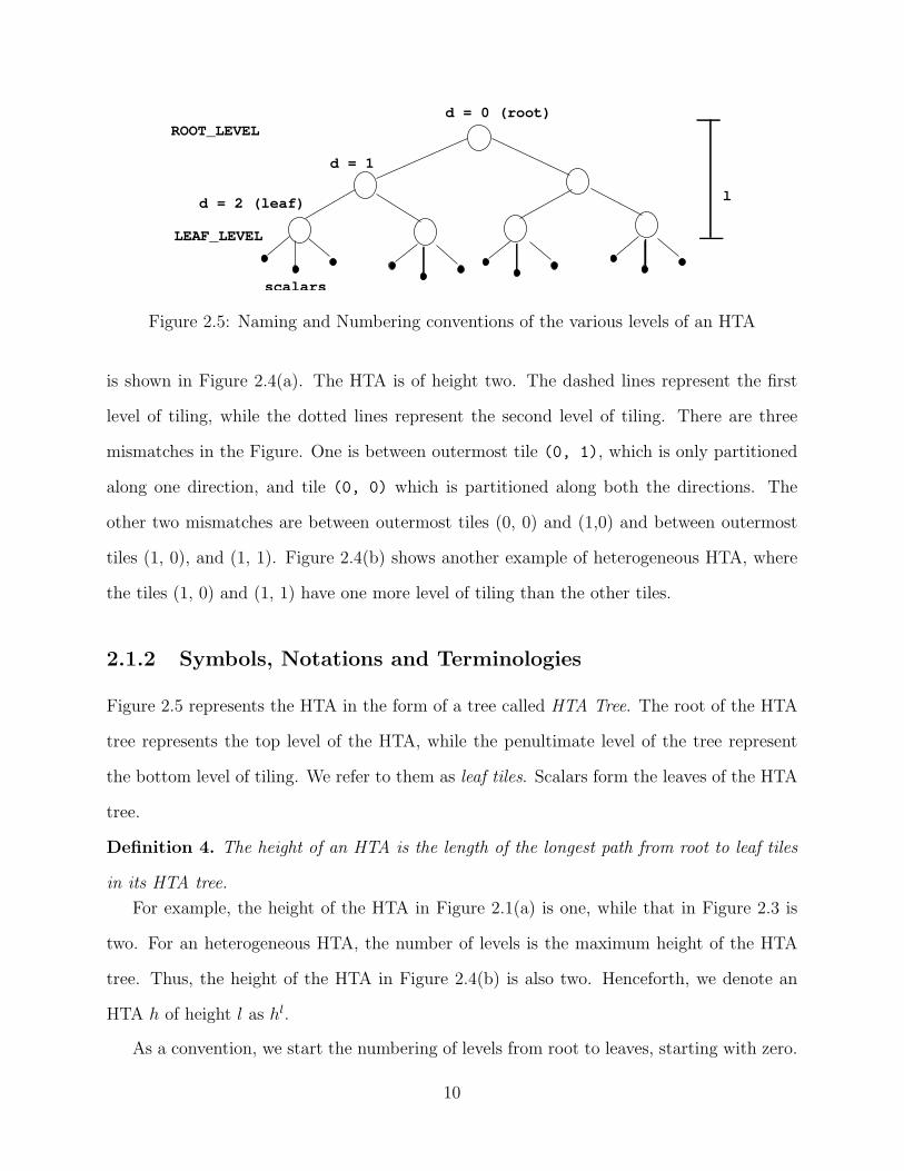
Figure 2.5: Naming and Numbering conventions of the various levels of an HTA
is shown in Figure 2.4(a). The HTA is of height two. The dashed lines represent the first
level of tiling, while the dotted lines represent the second level of tiling. There are three
mismatches in the Figure. One is between outermost tile (0, 1), which is only partitioned
along one direction, and tile (0, 0) which is partitioned along both the directions. The
other two mismatches are between outermost tiles (0, 0) and (1,0) and between outermost
tiles (1, 0), and (1, 1). Figure 2.4(b) shows another example of heterogeneous HTA, where
the tiles (1, 0) and (1, 1) have one more level of tiling than the other tiles.
2.1.2 Symbols, Notations and Terminologies
Figure 2.5 represents the HTA in the form of a tree called HTA Tree. The root of the HTA
tree represents the top level of the HTA, while the penultimate level of the tree represent
the bottom level of tiling. We refer to them as leaf tiles. Scalars form the leaves of the HTA
tree.
Definition 4. The height of an HTA is the length of the longest path from root to leaf tiles
in its HTA tree.
For example, the height of the HTA in Figure 2.1(a) is one, while that in Figure 2.3 is
two. For an heterogeneous HTA, the number of levels is the maximum height of the HTA
tree. Thus, the height of the HTA in Figure 2.4(b) is also two. Henceforth, we denote an
HTA h of height l as hl.
As a convention, we start the numbering of levels from root to leaves, starting with zero.
10
Thus, the root of the HTA is at level zero, while the leaf tiles have the level equal to the height
of the tree. To simplify our explanation, we include three variables SCALAR LEV EL,
LEAF LEV EL and ROOT LEV EL to indicate the level of the scalars, leaves and root
respectively.
Definition 5. We call the components of an HTA an element. An element of an HTA hl
is an HTA rl−1 or an array of scalars or a scalar.We also use the following four terminologies that are not related to HTA, but are used
in the HTA construction and operations : tuple, range, region and dist.
A tuple is an n-dimensional index value from Zn. We represent a tuple as i0, i1..in−1.
range is a range of integers in the closed interval [low, end], with optional step. A range
is represented as low : high[: step].
region is an n-dimensional rectangular index space spanned by n ranges. A region of
n dimensions is represented by a list of n comma separated ranges (e.g. 1 : 4 : 1, 1 : 8 : 1).
The size of a region is given by an n-tuple (d0, d1, ..., dn−1), where each di is the number
of elements in the ith range. A n-dimensional region of size (d0, d1, ..., dn−1) has d0 ×
d1, ...,×dn−1 index points : {(i0, i1, ..., in−1),∀i0 = 0, ..., d0 − 1,∀i1 = 0, ..., d1 − 1, ...,∀in−1 =
0, ..., dn−1 − 1)}. For simplicity, we refer to the set of index points as i0, i1, ...in−1, with an
implicit assumption of ∀ for each of the index symbols. We refer to the set of index points of
the region as index space. For example, the region 1 : 4 : 2, 1 : 4 : 2, has the index space,
(1,1), (1,3), (3, 1), (3, 3).
The total number of elements in a region is known as its cardinality. For example, the
cardinality of the region (1 : 4, 1 : 4) is 16. We call the size of the region and the dimension
of the region collectively as its shape. shape can be viewed as a logical structure with two
values, the dimension and the size of the region. For example, the shape of 1 : 4 : 2, 1 : 8 : 2
is {2, [2, 4]}.
dist of type dist-type, is a function that maps each index point of a region to dif-
ferent processors. dist is represented as an n-dimensional array. The value of the dist at
position (i0, i1, ..., in−1) corresponds to the processor numbers to which the index position
11

region (0:3, 0:2) dist
(a) (b)
0 1 2
3 4 5
6 7 8
9 10 11rang
e (0
:3)
tuple (0,0)
tuple (3,2)
range (0:2)
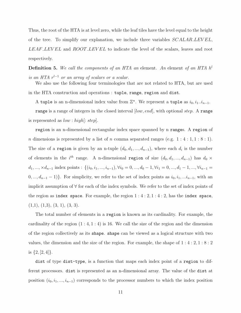
Figure 2.6: Illustration of (a) tuple, range, region and (b) dist
(i0, i1, ..in−1) of the region is mapped. The values are calculated according to dist-type.
Examples of dist-type are row-cyclic, column-cyclic and double-cyclic.
For simplicity, we use several syntactic short cuts. The open range (:), refers to the entire
range of an array. Open range by itself does not have any value, but when used in a context
of an array or HTA (e.g. a[:]), they refer to the entire range spanned by the corresponding
dimension of the array. That is, a[:] is the syntactic short cut for a[lb0 : ub0 : 1]. : can
be used in multiple positions of the array access operations. For example, a[:, :] refers to
a[lb0 : ub0, lb1 : ub1], where lbi and ubi are lower and upper bound of dimension i. For the
discussions in this chapter, we also assume 0-origin indexing for all the elements in an array
or an HTA.
Figure 2.6 illustrates these 4 objects graphically. In the Figure 2.6(a), the region is a
space spanned by the ranges (0 : 3, 0 : 2). Thus, the region is a 2-dimensional region of size
(4,3). Each point in the region is numbered in lexicographic order starting with the top-
left corner and traversing in row major order. The region is distributed using row-cyclic
distribution on 12 processors. The resulting distribution is shown in the Figure 2.6(b).
12
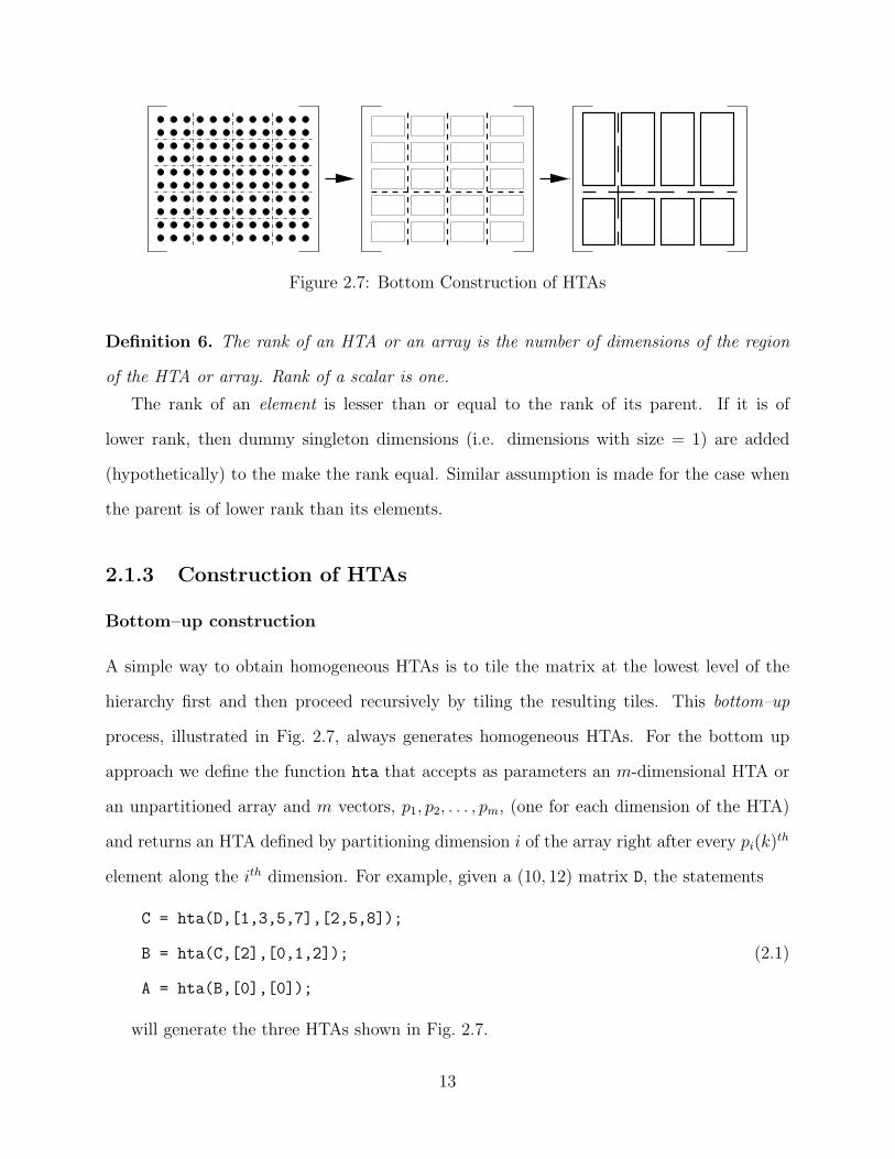
Figure 2.7: Bottom Construction of HTAs
Definition 6. The rank of an HTA or an array is the number of dimensions of the region
of the HTA or array. Rank of a scalar is one.
The rank of an element is lesser than or equal to the rank of its parent. If it is of
lower rank, then dummy singleton dimensions (i.e. dimensions with size = 1) are added
(hypothetically) to the make the rank equal. Similar assumption is made for the case when
the parent is of lower rank than its elements.
2.1.3 Construction of HTAs
Bottom–up construction
A simple way to obtain homogeneous HTAs is to tile the matrix at the lowest level of the
hierarchy first and then proceed recursively by tiling the resulting tiles. This bottom–up
process, illustrated in Fig. 2.7, always generates homogeneous HTAs. For the bottom up
approach we define the function hta that accepts as parameters an m-dimensional HTA or
an unpartitioned array and m vectors, p1, p2, . . . , pm, (one for each dimension of the HTA)
and returns an HTA defined by partitioning dimension i of the array right after every pi(k)th
element along the ith dimension. For example, given a (10, 12) matrix D, the statements
C = hta(D,[1,3,5,7],[2,5,8]);
B = hta(C,[2],[0,1,2]); (2.1)
A = hta(B,[0],[0]);
will generate the three HTAs shown in Fig. 2.7.
13

h = topdown(2);
function h = topdown (level)
if (level == LEAF_LEVEL)
h = rand(4,4);
else
h = hta(2,2);
for i = 1:2
for j = 1:2
h(i, j) = topdown (level-1);
end
end
end
Figure 2.8: Top–down HTA construction (a MATLAB like pseudo-code)
Top–down construction
We can alternatively start from the top and successively refine each partition. This top down
approach is more flexible than the bottom up approach in that it enables the generation of
both homogeneous and heterogeneous HTAs. HTAs are created top down using recursion.
First, an empty HTA is created. To create an empty HTA the following constructor is used:
hta(size0, size1,...sized−1)
In the above constructor, the arguments represent the size along each dimension of the
top level of the HTA. After the empty top level HTA is created, each of its tiles can be
initialized to contain either an HTA or a matrix. Before presenting an example of top down
creation of HTAs, we need to describe how to address the tiles in an HTA. The outermost
tiles of an HTA can be addressed using subscripts enclosed within parenthesis. An additional
set of subscript should be added for each level of the HTA that needs to be addressed. More
details on selection operation will be provided later. For now, the reader should only be
informed that ’()’ selects a tile at a given index position. A MATLAB like psuedo-code of
the top down creation of an HTA of Figure 2.3 is shown in the Figure 2.8.
Bottom up creation always generates an homogeneous HTA. It is useful to convert existing
arrays to HTAs. A drawback of the bottom up approach is that it creates intermediate HTAs
which are in most cases unnecessary. A compiler or a garbage collector could have these
temporary HTAs deleted after their only use in the creation sequence or could avoid their
14
creation altogether by, for example, reversing the creation process into a top down form.
Top down creation is preferred for parallel programs, as it does not require the entire
array to be allocated before the HTA is created; each processor can allocate only the tiles it
owns. Moreover, top down creation allows both heterogeneous and homogeneous HTAs to
be built in a similar fashion.
Special HTA constructors
Since homogeneous HTAs are the most widely used HTAs, an HTA constructor that con-
structs any level homogeneous HTA is also provided. This constructor accepts only the size
of the tiles at each level of the hierarchy:
C = hta ((d0, d1, ..dd−1)0,...(d0, d1, ..dd−1)
l);
Each of the argument in the above constructor is a tuple of size d. Argument i specifies
the size of the tiles at level i.
2.2 HTA Operations
A fundamental idea in the design of array languages is that any operation defined on scalars
can be extended to apply element-by-element to an array of scalars [37]. We extend this
concept to HTAs, by extending the operations defined on arrays of scalars to arrays of tiles.
The operations defined on arrays of scalars are extended to operate recursively on each of
the element of an HTA. The result of the operations depends on the shape and the tiling
hierarchy of the HTA and the level of the application of the operation. In the following
sections, we define the set of operations defined for HTAs. Readers are advised that most
of the operations are defined only for homogeneous HTAs. Extending the semantics of the
operations to heterogeneous HTAs is left as a future work.
15
, , or
h(1,0)
h(1,0)(0,1)[0,1] or h(1,0)[0,3]h[4,3]
h(0,0:1)
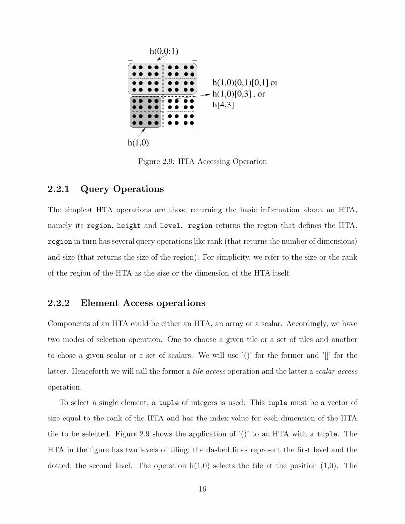
Figure 2.9: HTA Accessing Operation
2.2.1 Query Operations
The simplest HTA operations are those returning the basic information about an HTA,
namely its region, height and level. region returns the region that defines the HTA.
region in turn has several query operations like rank (that returns the number of dimensions)
and size (that returns the size of the region). For simplicity, we refer to the size or the rank
of the region of the HTA as the size or the dimension of the HTA itself.
2.2.2 Element Access operations
Components of an HTA could be either an HTA, an array or a scalar. Accordingly, we have
two modes of selection operation. One to choose a given tile or a set of tiles and another
to chose a given scalar or a set of scalars. We will use ’()’ for the former and ’[]’ for the
latter. Henceforth we will call the former a tile access operation and the latter a scalar access
operation.
To select a single element, a tuple of integers is used. This tuple must be a vector of
size equal to the rank of the HTA and has the index value for each dimension of the HTA
tile to be selected. Figure 2.9 shows the application of ’()’ to an HTA with a tuple. The
HTA in the figure has two levels of tiling; the dashed lines represent the first level and the
dotted, the second level. The operation h(1,0) selects the tile at the position (1,0). The
16

result is a HTA of height l − 1, where l is the height of the original HTA.
A region can also be used in the () operation. Selection of a region from an HTA
results in another HTA of same level, but shape of that of the region. In the example, h(0,
0:1) will select the entire first row tiles from h. Thus, the result in the example is a HTA of
height l and shape {2, (1, 2)}.
The operation [] selects a given scalar or a region of scalars from the HTA like a normal
array. The indices used in this selection are global. That is, the indices do not take in
to account the tiling hierarchy and the HTA is just treated as a normal array with the
underlying scalars being its elements.In the given example, h[4,3] selects the scalar value
from that position.
The scalar selection operation can be applied to any level of an HTA. For example, other
ways to access the same scalar are h(1,0)[0,3] and h(1,0)(0,1)[0,1]. Here, one ore more ’()’
and ’[]’ are chained together. Such chaining of () is allowed to a maximum length equal
to the height of the HTA. The last of such a chain can be a ’[]’ operator. Each ’()’ or ’[]’
operation is applied locally to each of the tiles selected by the preceding ’()’ operation. Since
operator () can be chained we also call it hierarchical access operation to distinguish from
operator [], which can not be chained. We call operator [] a flat operator. The process of
applying [] to an HTA is known as flattening. Flattening converts an HTA in to a normal
flat array without any tiling hierarchy.
The access operations can also take as its input a vector of subscripts v0, v1, ...vn−1, one
each for each dimension of the HTA. The result is an HTA of size (lenght(v0), ....length(vn−1)).
Each element in the HTA is selected using an index space in the Cartesian product set of
v0, v1, ..vn−1. For example, if h is an HTA of size (5, 4), the statement
h([1, 3],[1, 2])
selects the elements at the following positions (in the same order) : (1, 1), (1, 2), (3, 1), (3, 2).
This the most general HTA access. The access operations that use region and tuple are
specific instances of this operation.
17

0 0 1 0
1 0 0 00 1 0 0
0 0 0 10 0 1 1
1 1 1 1
0 1 1 1
0 0 0 1
index = index =
h{index} h{index}
(a) (b)
Figure 2.10: Logical Indexing of HTAs
A special case of access operation is where the input can be a matrix of boolean values.
Such a matrix should be of same rank and size as that of the HTA h. The result of the
selection operation using such a boolean matrix, is also an HTA of same shape, with the
tiles corresponding to the false positions of the boolean matrix being empty. Figure 2.10(a)
shows an example of selecting a diagonal of an hta h using a boolean matrix. Figure 2.10(b)
shows an example of selecting a upper triangular section from a HTA.
2.2.3 Point-wise operations
This set of operations deals with those operations that affect each of the scalar values of
the HTA. The outcome of these operations do not depend on the order of application of the
operations to the individual elements of the HTA. That is, the elements can be visited in
any iteration order. However, the order should be the same for all the operand HTAs.
18

struct plus {
double operator() (const double a,
const double b) {
return a+b;
}
}
Primitive operations
All the HTA operations are described in terms of primitive scalar operations. Example of
the primitive operations is any arithmetic operation. We use STL-like functor objects for
describing the primitive operators as shown in the Figure 2.2.3. Here, plus is the scalar
binary addition operation.For simplicity, we use symbols like +, -, *, / etc., for well known
binary operations like addition, subtraction, multiplication, division, etc.,
Unary Operations
An unary operation on an HTA can be generalized as:
rl = op(hl) ≡ r(i0, i1, ...in−1)l−1 = op(h(i0, i1, ...in−1)
l−1)
Examples of unary operations are unary minus, logical negation etc.
Binary Operations
HTAs can be operated using binary operations, like addition. Binary operations require their
operands to be conformable. This is required to provide a consistent definition of operations
without any ambiguity. If two operand HTAs have same height and the same shape at every
level, then corresponding scalar elements can be operated. Ambiguity arises when shape and
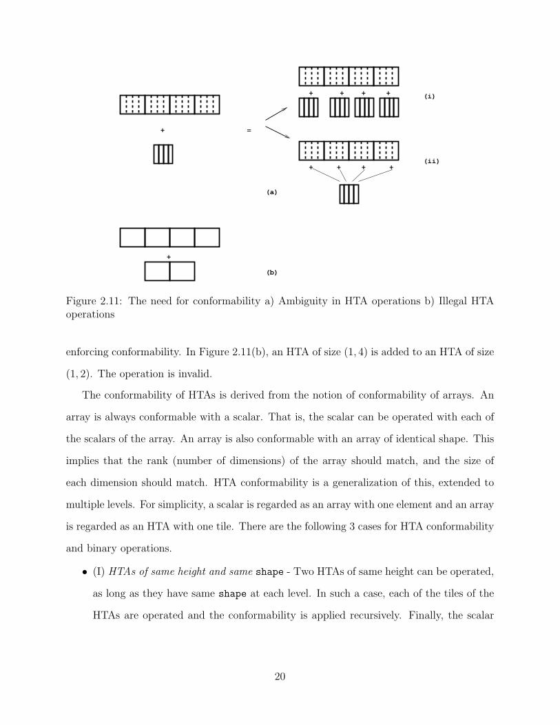
height are not identical. For example, Figure 2.11(a) shows a case of ambiguity in operating
two HTAs. Here a HTA of height two is added to an HTA of height one. There are 2
possibilities - the HTA of height one can be replicated and operated with each of the tiles
of the other HTA (case (i)) or each tile of the HTA of height one can be added individually
to each of the tiles of the other HTA (case (ii)). Validity of operations is another reason for
19
=+
+ + + +
++++
+
(a)
(b)
(i)
(ii)
Figure 2.11: The need for conformability a) Ambiguity in HTA operations b) Illegal HTAoperations
enforcing conformability. In Figure 2.11(b), an HTA of size (1, 4) is added to an HTA of size
(1, 2). The operation is invalid.
The conformability of HTAs is derived from the notion of conformability of arrays. An
array is always conformable with a scalar. That is, the scalar can be operated with each of
the scalars of the array. An array is also conformable with an array of identical shape. This
implies that the rank (number of dimensions) of the array should match, and the size of
each dimension should match. HTA conformability is a generalization of this, extended to
multiple levels. For simplicity, a scalar is regarded as an array with one element and an array
is regarded as an HTA with one tile. There are the following 3 cases for HTA conformability
and binary operations.
• (I) HTAs of same height and same shape - Two HTAs of same height can be operated,
as long as they have same shape at each level. In such a case, each of the tiles of the
HTAs are operated and the conformability is applied recursively. Finally, the scalar
20

elements of the HTAs are operated.
rl = hl � vl ≡ r(i0, i1..in−1)l−1 = h(i0, i1..in−1)
l−1 � v(i0, i1..in−1)l−1
• (II) HTAs of same height and different shape - Two HTAs with the same height, but
different shape, can be operated iff the region of one of the HTAs has cardinality one.
In this case, the HTA with the region of cardinality one is operated with each of the
tiles of the other HTA, recursively. Logically, the single element HTA is promoted to
an HTA of same shape as that of the other HTA by (logical) replication. We refer to
this as argument expansion.
rl = hl � ul ≡
r(i0, i1..in−1)
l−1 = h(i0, i1..in−1)l−1 � u(0)l−1, if card(u) = 1
r(i0, i1..in−1)l−1 = h(i0, i1..in−1)
l−1 � u(i0, i1...in−1)l−1, otherwise
• (III) HTAs of different height - Two HTAs of different height, hl and vm, with l > m,
are conformable iff the HTA of lower-level is recursively conformable with each of the
tiles of the HTA of higher level. That is, the HTA of level m is (logically) promoted to
an HTA of the level l, by wrapping the original HTA with dummy singleton levels of
tiling. We refer to this as boxing. This is followed by the application of rule II. Boxing
always precedes argument expansion.
rl = hl � um ≡
r(i0, i1, ...in−1)
l−1 = h(i0, i1, ...in−1)l−1 � vm, if l > m
rl = hl � vl, otherwise
(2.2)
Figure 2.12 illustrates the above cases graphically. Figure 2.12(b) shows the argument
expansion, where an HTA with one element is logically promoted to the same shape as that
of the LHS operand. Figure 2.12(c) shows boxing, where an HTA of height one is logically
promoted to an HTA of height two by adding dummy tiling of size one along each dimension.
21

=
=
(III)
(II)
(I)
=
Figure 2.12: An illustration of the HTA rules of operation
This is followed by the application of argument expansion and rule (II).
Algorithm 1 lists the algorithm for the conformability check during a binary operation.
The algorithm implements the 3 cases of HTA binary operation discussed earlier. In the
Algorithm, d0, ..dn−1 represent the size of the each dimension of the region of the HTA.
Here we assume all the HTAs have same region (i.e., same index space) also, apart from
shape. This is not a necessary condition. For HTAs whose regions have different index
spaces, we should iterate each HTA using the iterator of its region.
Algorithm 2 lists the sequence of steps performed by a binary operation, before it invokes
the conformability check. The Algorithm 2 interchanges the argument to Algorithm 1 such
that its argument h has height and number of elements larger than or equal to v. op scalar
is the final scalar routine that implements the op for scalar values.
The conformability check is applied before every point-wise operations and assignments.
An operation between two non conformable HTAs is illegal. The programmer is responsible
for creating conformable HTAs before operating them. Creation of the HTA that results
after the binary operation is itself a binary operation and should be performed using the
same algorithm as above.
22

Algorithm 1 binary op (op, r, h, v)
1: h and v are left and right HTAs of a binary operation. r is the result HTA.2: if height(h) = height(v) then3: if region(h) = region(v) then4: (case I)5: for i0 = 0 to d0 − 1 do6: for i1 = 0 to d1 − 1 do
7:...
8: for in−1 = 0 to dn−1 − 1 do9: op (r(i0, i1, ..., in−1), h(i0, i1, ..., in−1), v(i0, i1, ...in−1))
10: end for11: end for12: end for13: else14: (case II)15: for i0 = 0 to d0 − 1 do16: for i1 = 0 to d1 − 1 do
17:...
18: for in−1 = 0 to dn−1 − 1 do19: op (r(i0, i1, ..., in−1), h(i0, i1, ..., in−1), v(0))20: end for21: end for22: end for23: end if24: else25: (case III)26: for i0 = 0 to d0 − 1 do27: for i1 = 0 to d1 − 1 do
28:...
29: for in−1 = 0 to dn−1 − 1 do30: op (r(i0, i1, ..., in−1), h(i0, i1, ..., in−1), v)31: end for32: end for33: end for34: end if
23
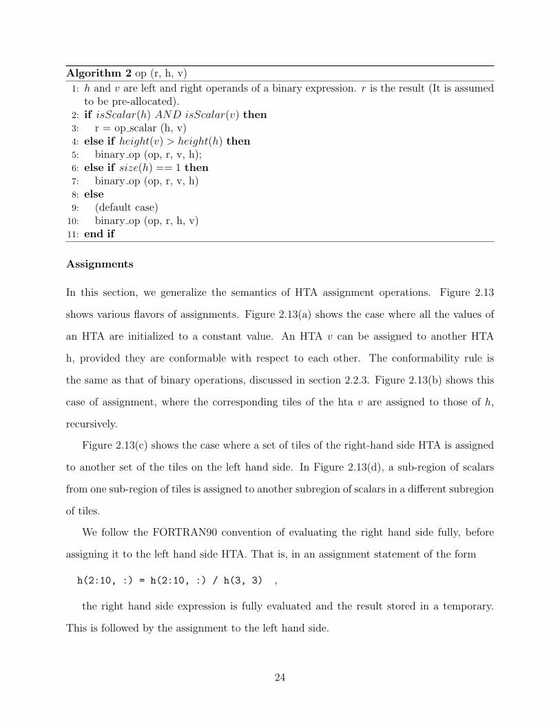
Algorithm 2 op (r, h, v)
1: h and v are left and right operands of a binary expression. r is the result (It is assumedto be pre-allocated).
2: if isScalar(h) AND isScalar(v) then3: r = op scalar (h, v)4: else if height(v) > height(h) then5: binary op (op, r, v, h);6: else if size(h) == 1 then7: binary op (op, r, v, h)8: else9: (default case)
10: binary op (op, r, h, v)11: end if
Assignments
In this section, we generalize the semantics of HTA assignment operations. Figure 2.13
shows various flavors of assignments. Figure 2.13(a) shows the case where all the values of
an HTA are initialized to a constant value. An HTA v can be assigned to another HTA
h, provided they are conformable with respect to each other. The conformability rule is
the same as that of binary operations, discussed in section 2.2.3. Figure 2.13(b) shows this
case of assignment, where the corresponding tiles of the hta v are assigned to those of h,
recursively.
Figure 2.13(c) shows the case where a set of tiles of the right-hand side HTA is assigned
to another set of the tiles on the left hand side. In Figure 2.13(d), a sub-region of scalars
from one sub-region of tiles is assigned to another subregion of scalars in a different subregion
of tiles.
We follow the FORTRAN90 convention of evaluating the right hand side fully, before
assigning it to the left hand side HTA. That is, in an assignment statement of the form
h(2:10, :) = h(2:10, :) / h(3, 3) ,
the right hand side expression is fully evaluated and the result stored in a temporary.
This is followed by the assignment to the left hand side.
24

1.0 1.01.0 1.01.01.0
1.01.0
1.0 1.01.0 1.01.01.0
1.01.0
h(:, :) = 1.0
h(:,:) = v(:, :)
h(:, 0) = v(:, 1)
h(0, :)[2, :] = h(1, :)[1,:]
h v
h v
(a)
(b)
(c)
(d)
h
h
Figure 2.13: HTA Assignments
2.2.4 Collective Operations
This class of operations includes all the operations that do not change the values of the
scalar elements of the HTA, but their positions in the HTA. They also alter the positions of
the elements in the other levels of the HTA. Thus, these operations change the structure of
the HTA.
25
1 2 3 4 5 6
11 12 13 14 15 16
17 18 19 20 21 22
7 8 9 10 11 12
1 7 11 17
2 8 12 18
3 9 13 19
4 10 14 20
5 11 15 21
6 12 16 22
1 2 3 4 5 6
11 12 13 14 15 16
17 18 19 20 21 22
7 8 9 10 11 12
1 7 11 17
2 8 12 18
3 9 13 19
4 10 14 20
5 11 15 21
6 12 16 22
1 2 11 12 7 8 17 18
9 10 11 12
3 4 5 6
13 14 15 16
19 20 21 22
(a)h.transpose()
1 2 3 4 5 6
11 12 13 14 15 16
17 18 19 20 21 22
7 8 9 10 11 12
1 7 11 17
2 8 12 18
3 9 13 19
4 10 14 20
5 11 15 21
6 12 16 22
(b)
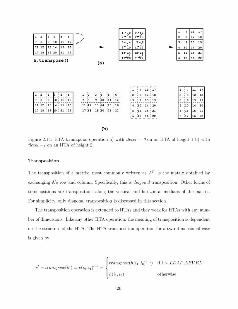
Figure 2.14: HTA transpose operation a) with tlevel = 0 on an HTA of height 1 b) withtlevel =1 on an HTA of height 2.
Transposition
The transposition of a matrix, most commonly written as AT , is the matrix obtained by
exchanging A’s row and column. Specifically, this is diagonal transposition. Other forms of
transpositions are transpositions along the vertical and horizontal medians of the matrix.
For simplicity, only diagonal transposition is discussed in this section.
The transposition operation is extended to HTAs and they work for HTAs with any num-
ber of dimensions. Like any other HTA operation, the meaning of transposition is dependent
on the structure of the HTA. The HTA transposition operation for a two dimensional case
is given by:
vl = transpose(hl) ≡ v(i0, i1)l−1 =
transpose(h(i1, i0)
l−1) if l > LEAF LEV EL
h(i1, i0) otherwise
26
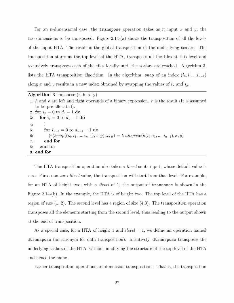
For an n-dimensional case, the transpose operation takes as it input x and y, the
two dimensions to be transposed. Figure 2.14-(a) shows the transposition of all the levels
of the input HTA. The result is the global transposition of the under-lying scalars. The
transposition starts at the top-level of the HTA, transposes all the tiles at this level and
recursively transposes each of the tiles locally until the scalars are reached. Algorithm 3,
lists the HTA transposition algorithm. In the algorithm, swap of an index (i0, i1, ...in−1)
along x and y results in a new index obtained by swapping the values of ix and iy.
Algorithm 3 transpose (r, h, x, y)
1: h and v are left and right operands of a binary expression. r is the result (It is assumedto be pre-allocated).
2: for i0 = 0 to d0 − 1 do3: for i1 = 0 to d1 − 1 do
4:...
5: for in−1 = 0 to dn−1 − 1 do6: (r(swap((i0, i1, ..., in−1), x, y), x, y) = transpose(h(i0, i1, ..., in−1), x, y)7: end for8: end for9: end for
The HTA transposition operation also takes a tlevel as its input, whose default value is
zero. For a non-zero tlevel value, the transposition will start from that level. For example,
for an HTA of height two, with a tlevel of 1, the output of transpose is shown in the
Figure 2.14-(b). In the example, the HTA is of height two. The top level of the HTA has a
region of size (1, 2). The second level has a region of size (4,3). The transposition operation
transposes all the elements starting from the second level, thus leading to the output shown
at the end of transposition.
As a special case, for a HTA of height 1 and tlevel = 1, we define an operation named
dtranspose (an acronym for data transposition). Intuitively, dtranspose transposes the
underlying scalars of the HTA, without modifying the structure of the top-level of the HTA
and hence the name.
Earlier transposition operations are dimension transpositions. That is, the transposition
27
�������������������������������� ���������
����������������������� �������
��������������������� �������
�������������������������
�������������������
�����������������������
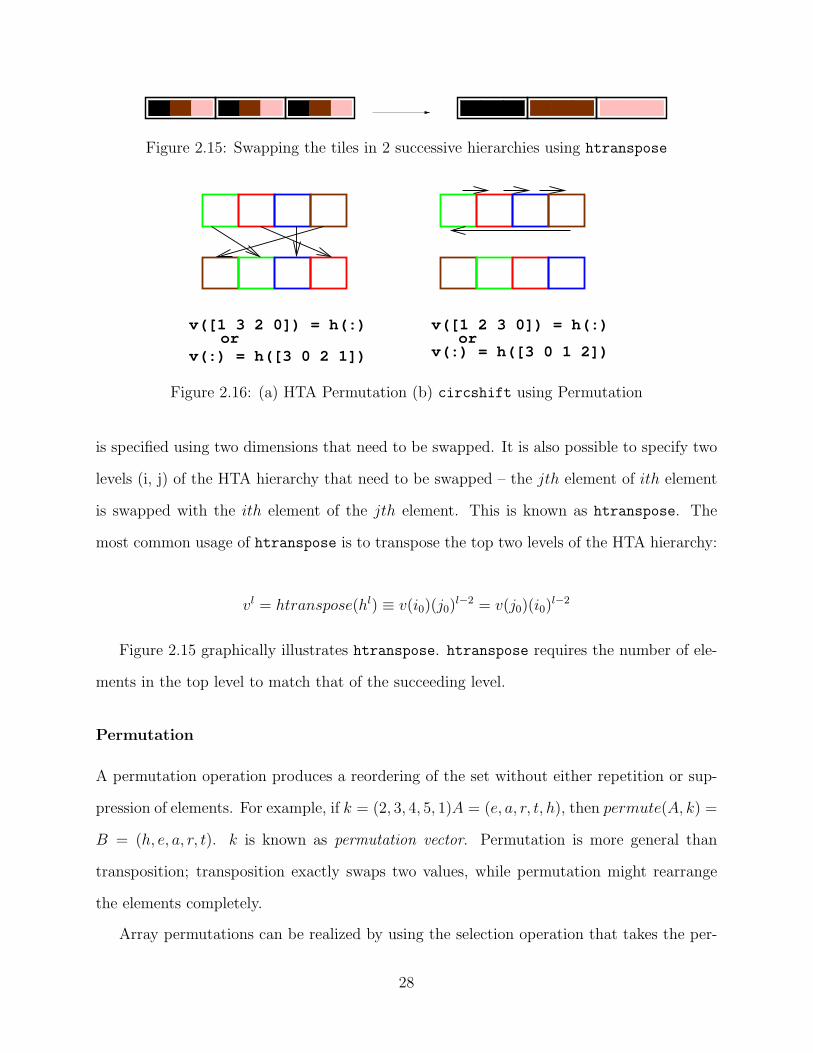
Figure 2.15: Swapping the tiles in 2 successive hierarchies using htranspose
ororv([1 3 2 0]) = h(:)
v(:) = h([3 0 2 1])
v([1 2 3 0]) = h(:)
v(:) = h([3 0 1 2])
Figure 2.16: (a) HTA Permutation (b) circshift using Permutation
is specified using two dimensions that need to be swapped. It is also possible to specify two
levels (i, j) of the HTA hierarchy that need to be swapped – the jth element of ith element
is swapped with the ith element of the jth element. This is known as htranspose. The
most common usage of htranspose is to transpose the top two levels of the HTA hierarchy:
vl = htranspose(hl) ≡ v(i0)(j0)l−2 = v(j0)(i0)
l−2
Figure 2.15 graphically illustrates htranspose. htranspose requires the number of ele-
ments in the top level to match that of the succeeding level.
Permutation
A permutation operation produces a reordering of the set without either repetition or sup-
pression of elements. For example, if k = (2, 3, 4, 5, 1)A = (e, a, r, t, h), then permute(A, k) =
B = (h, e, a, r, t). k is known as permutation vector. Permutation is more general than
transposition; transposition exactly swaps two values, while permutation might rearrange
the elements completely.
Array permutations can be realized by using the selection operation that takes the per-
28

0 11 0
0 11 0
0 11 0
0 11 0
0 11 0
0 11 0
0 11 0
0 11 0
0 11 0
0 11 0
0 11 0
0 11 0
0 11 0
0 11 0
0 11 0
0 11 0
0 11 0
0 11 0
0 11 0
0 11 0
0 11 0
0 11 0
0 11 0
0 11 0 0 11 0
(a)
(b)
repmat (h, 0, [2 2])
repmat (a, [2 2])
Figure 2.17: Replication of Tiles of an HTA using repmat
mutation vector as its input. For example, the above permutation can be realized by:
B(k) = A; or B = A(i), where i = (5, 1, 2, 3, 4);
The permutation operation is extended to HTAs, where in the tiles can be permuted using
the permutation vector and the selection operation. Figure 2.16-(a) shows an example of
permuting the top level tiles of an HTA.
Each of the levels of the HTA can be permuted independent of the other by chaining
several ’()’ and providing a permutation vector for each selection operation.
Permutation is a very general operation, and can be used to realize several other common
operations. As stated earlier, transposition is a special case of permutation. Another example
is circular shift, which shifts the elements of an HTA in a given direction by given offset.
This is shown in Figure 2.16-(b). As a syntactic short cut, the circular shift is generalized
as another operation. This operation, circshift, takes as its input the direction vector (d),
where size(d) = rank(h). Each element di of the direction vector specifies the offset (+x or
-x) of shift for the dimension i.
29

Replication
Replication of elements of a matrix is useful in certain applications. The repmat function,
inspired from MATLAB, accomplishes this. In MATLAB, the statement B = repmat(A,
[m,n]), where A is an array with region of size (d0, d1), creates a large matrix B consisting
of an m-by-n tiling of copies of A. The size of B is (d0 ∗ m, d1 ∗ n). B = repmat(A,[m n
p...]), where A is an array with region of size (d0, d1, ..dn−1), produces a multidimensional
array B composed of copies of A. The size of B is (d0 ∗m, d1 ∗ n, d2 ∗ p, ...).
The repmat function is extended to HTAs, where in they replicate the tiles. Like
other operations, repmat is also parameterized by recursion level, whose default value is
LEAF LEVEL. Figure 2.17(a) shows the replication of the top level tiles of a HTA of height
one. In the Figure, the recursion level for repmat is zero (root). The result is an HTA that
consists of (2, 2) copies of the original (2, 2) HTA. Thus, the result HTA is a (4, 4) HTA.
2.2.5 Higher-order Operators
HTAs can be operated with the following higher-order operators: map, reduce and scan.
Higher-order operators are parametrized with primitive operators and define the strategy
and result format resulting from the application of primitive operators to the tiles or scalar
values in an HTA. Using these higher-order operations it is possible to obtain new HTA
operations like summation or sorting of an HTA.
Map
map applies a function f to each one of the elements of the input HTA at a given level.
The syntax of map is shown in Figure 2.18, along with examples. In the figure, h = ((n,
m ),..., (x, y)) indicates the region of each level of the HTA h from leaf to root. map
takes as input an op, and a level rlevel. The rlevel specifies the level of the HTA at which
op will be invoked. The default value of rlevel is SCALAR LEV EL. Invocation of map
on HTA h, results in the map function being invoked on the top level of h. If its elements
30

h = (2x2,2x2)
sin
sin
sin
sin
sin
sin
sin
sin
sin
sin
sin
sin
sin
sin
sin
sin
h = (2x2,2x2)
map (op, h[, mlevel])
map(sin(), h)
ft ft ft
ft ft ft
h = (1x2, 1x2, 1x3) h = (1x2, 1x2, 1x3)
map(ft(0), h, 2)
Figure 2.18: HTA map operator
are tiles themselves, then the function is invoked recursively on each of their elements until
level = SCALAR LEV EL or level = rlevel. The op is invoked over the elements of the
HTA at that level. If the element is an array, a function that takes array as its input is
invoked.If the element is an HTA, then a function that takes HTA at its input is invoked, if
available. Otherwise, it is cast in to an array (by flattening) and the function that takes an
array as its input is invoked. If no such function exists, then an exception should be thrown.
The order of iteration in the map does not affect the result of the computation. The op
can be any primitive function or a reduce or a scan (discussed in the following sections).
Though not shown in the figure, map can also take one or more HTAs as its argument, along
with op. The argument HTAs should have the same shape until level = rlevel and should
be of same height.
map forms the basis for several point-wise HTA operations. For example, scalar addition
of two HTAs, h1 and h2 (with same region and same height), is implemented using map as
follows: r = map(plus, h1, h2);
The structure and the shape of the output HTA depends on the type of the operation (op)
31

0 1 1 01 0 0 1
021 1
111 1
2222
2222
1 0 1 0 0 0 1 1
1 0 1 0 0 0 1 1
0 1 1 01 0 0 1
+
+ ++
reduce(plus(), h, 1, 0)
reduce(plus(), h, 1, 1)
reduce (op, h[, dim, [rlevel]])
Figure 2.19: HTA reduce operator
and the level of its application (rlevel). In the examples shown in Figure 2.18, the output
of the map operation is the same as the input as the op does not change the structure of its
input data in both the cases and the rlevel is either SCALAR LEV EL or LEAF LEV EL.
In case (a), the op is the trigonometric sine function (sin), and level is SCALAR LEV EL.
That is, the sin function is applied to each of the scalar values of the input HTA. In case
(b), the op is the Fourier transform function and the rlevel is LEAF LEV EL. Fourier
transform is a vector function. Application of Fourier transform on a array results in the
Fourier transform of each its vector along the dimension dim. The dimension is specified as
an argument to the ft function.
Reduce
An operation which is applied to all components of a vector to produce a scalar is called
a reduction. For example, reduce(+, x) is sum and reduce(×, x) is product of a vector x.
The reduction operation can be generalized for n-dimensional arrays, resulting in an (n-1)-
dimensional arrays.
32

The reduction operation of arrays is extended to HTAs in the form of the reduce oper-
ation. Like map, reduce is also a recursive operation. The reduce will be applied to each
level recursively until the scalars are reached. Reduction on scalars is an identity function
that returns itself. After this, the reverse process of combining the values is performed. The
combining function is the op. The number of dimensions in the of elements in the result will
be reduced by one for all the levels. If the dimension argument is not specified, the reduction
occurs in all the dimension finally resulting in a scalar as the output. We call such a reduc-
tion full reduction as opposed to partial reduction along a given dimension. Moreover, the
HTA reductions are parameterized by level of recursion. This controls the height to which
the reduction has to proceed. In general, the reduction on an HTA of level l (with recursion
level being SCALAR LEV EL) and an operator op can be expressed as follows:
vl = reduce(op, hl, 0) ≡ v(0, i1, ..., in−1)l−1 =
reduce(op, h(0, i1...in−1)
l−1, 0)op ...
reduce(op, h(d0 − 1, ...in−1)l−1, 0)
(2.3)
In the above equation, it is assumed that the reduction is performed along the dimen-
sion 0. Reductions along other dimensions are analogous. The syntax of the HTA reduce
operation is:
reduce(op, h, [, dim [,rlevel]])
where,
• op: This is any associative operation from the set of primitive operations. Examples
are scalar addition, array addition, HTA addition, etc.
• dim: This is the dimension of reduction. All the levels of the HTA is reduced along
the same dimension.
• rlevel: This is the recursion level of the reduction. Default value is SCALAR LEVEL.
33

Figure 2.19 illustrates three kinds of reduction on an HTA of rank 2, level one and size
(2, 2). For simplicity, in all the cases we use plus (scalar addition) as the operator and the
dimension of the reduction is set to one. In the first case, the reduction results in an HTA of
size (2, 1). The reduction is applied to each tile of the HTA, and then the results are added
along the dimension one to produce the final result.
The second case is an example of stopping the reduction at a level other than the leaf.
In this case, the recursion is stopped at level = 0 (ROOT LEV EL). Only the top level tiles
are added along dim, resulting in a HTA of size (2, 1), whose tiles are of size (2, 2). A variety
of reductions can be obtained by controlling the above parameters.
Scan
scan computes the reductions of all the prefixes of a vector. For example, if the vector
v = (1, 2, 3, 4, 5), then scan(+, v) = (1, 3, 6, 10, 15). A similar scan is defined for HTAs also.
The syntax is very similar to that of reduce.
The syntax of the HTA scan operation is:
scan (op, h, [, dim [,rlevel]])
where,
• op: This is any primitive associative operation.
• dim: This is the dimension of scan.
• rlevel: This is the recursion level of the reduction. Default value is SCALAR LEVEL.
Figure 2.20 lists several examples of the HTA scan operation. In the example, the HTA
is of two levels and size (1, 3). Each of its tile are a HTA of height one and size (1, 2). The
leaves are of size (1, 2). For simplicity, we use the plus as our scan operation and one as the
dimension of scan. In the first case, the scan is invoked with rlevel of 2. So, the operation
proceeds till the scalar leaf elements. In the second case, the rlevel is 0 (root). Thus, all the
top level tiles are added cumulatively.
34

1 2 3 4 5 6 7 8 9 10 11 12
(a)
(b)
1 3 6 10 15 21 28 36 45 55 66 78
1 2 3 4 5 6 7 8 9 10 11 12
1 2 3 4 6 8 10 12 15 18 21 24
scan(plus(), h, 1, 0)
scan(plus(), h, 1, 2)
Figure 2.20: HTA scan operator
1 0 1 0 120
11
1
11
0 0 1 1
0 1 1 01 0 0 1
h.map(reduce(plus, 1), 1)
Figure 2.21: HTA reduce operator combined with map
2.2.6 Composing of operations
map can take any valid scalar, array or HTA operations as its input op. For instance, it is also
possible to use reduce as an argument to map operators. This will apply the reduction on a
per-tile basis. The level of the tile is chosen by the rlevel argument of the map. An example
is shown in Figure 2.21. Like reduce, scan can also be passed as an argument to map. An
1 2 3 4 5 6 7 8 9 10 11 12
1 3 3 7 5 11 7 15 9 19 11 23
map (scan(plus, 1), h, 2)
Figure 2.22: HTA scan operator combined with map
35
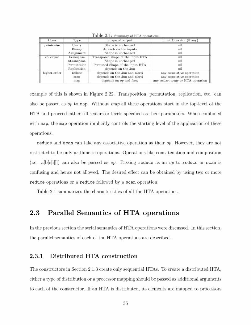
Table 2.1: Summary of HTA operations.
Class Type Shape of output Input Operator (if any)
point-wise Unary Shape is unchanged nilBinary depends on the inputs nil
Assignment Shape is unchanged nilcollective transpose Transposed shape of the input HTA nil
htranspose Shape is unchanged nilPermutation Permuted Shape of the input HTA nilReplication depends on the dim nil
higher-order reduce depends on the dim and rlevel any associative operationscan depends on the dim and rlevel any associative operationmap depends on op and level any scalar, array or HTA operation
example of this is shown in Figure 2.22. Transposition, permutation, replication, etc. can
also be passed as op to map. Without map all these operations start in the top-level of the
HTA and proceed either till scalars or levels specified as their parameters. When combined
with map, the map operation implicitly controls the starting level of the application of these
operations.
reduce and scan can take any associative operation as their op. However, they are not
restricted to be only arithmetic operations. Operations like concatenation and composition
(i.e. a[b[c[i]]]) can also be passed as op. Passing reduce as an op to reduce or scan is
confusing and hence not allowed. The desired effect can be obtained by using two or more
reduce operations or a reduce followed by a scan operation.
Table 2.1 summarizes the characteristics of all the HTA operations.
2.3 Parallel Semantics of HTA operations
In the previous section the serial semantics of HTA operations were discussed. In this section,
the parallel semantics of each of the HTA operations are described.
2.3.1 Distributed HTA construction
The constructors in Section 2.1.3 create only sequential HTAs. To create a distributed HTA,
either a type of distribution or a processor mapping should be passed as additional arguments
to each of the constructor. If an HTA is distributed, its elements are mapped to processors
36
according to the type of distribution.
The type of distribution (dist-type) is by default row-cyclic. That is, the elements of
the HTA are assigned one-to-one to the available processors in row-major order. If the num-
ber of processors is lesser than the number of elements, then the assignment of the remaining
elements start from the processor 0 and proceed again in row major order. The other valid
types of distribution are column-cyclic, block-cyclic and double-cyclic. The program-
mer can also specify the logical arrangement of processors along with the dist-type. We
call this processor topology. It is a n-tuple ( where n is the rank of the HTA) and each of its
value specifies the number of processors along that dimension. An example of topology is
[2, 2], which specifies that the processors are logically arranged in a (2, 2) mesh. If topology
is not specified the processors are just assumed to be arranged linearly.
If the type of the distribution is not one of the above, then the programmer can create
a processor mapping (dist – cf. Section 2.1.2) and supply as an argument to the HTA
constructors. We call the processor that owns a given element of an HTA the home node.
In this document, we restrict ourselves to HTAs whose top level (i.e., level = 0) only is
distributed. Extending the constructor and the other HTA operations to HTA whose other
levels are also distributed is left as a future extension.
2.3.2 Unary Operations
The semantics of unary operations are the same as that of serial execution. The computation
occurs in the home nodes of elements of the input HTA. If the number of elements in an
HTA is lesser than the number of processors, the processors that do not own the elements
do not participate in the unary operation.
2.3.3 Binary Operations
For parallel execution, the rules of conformability for binary operations of Section 2.2.3 are
augmented with the following additional rules of computation and communication:
37
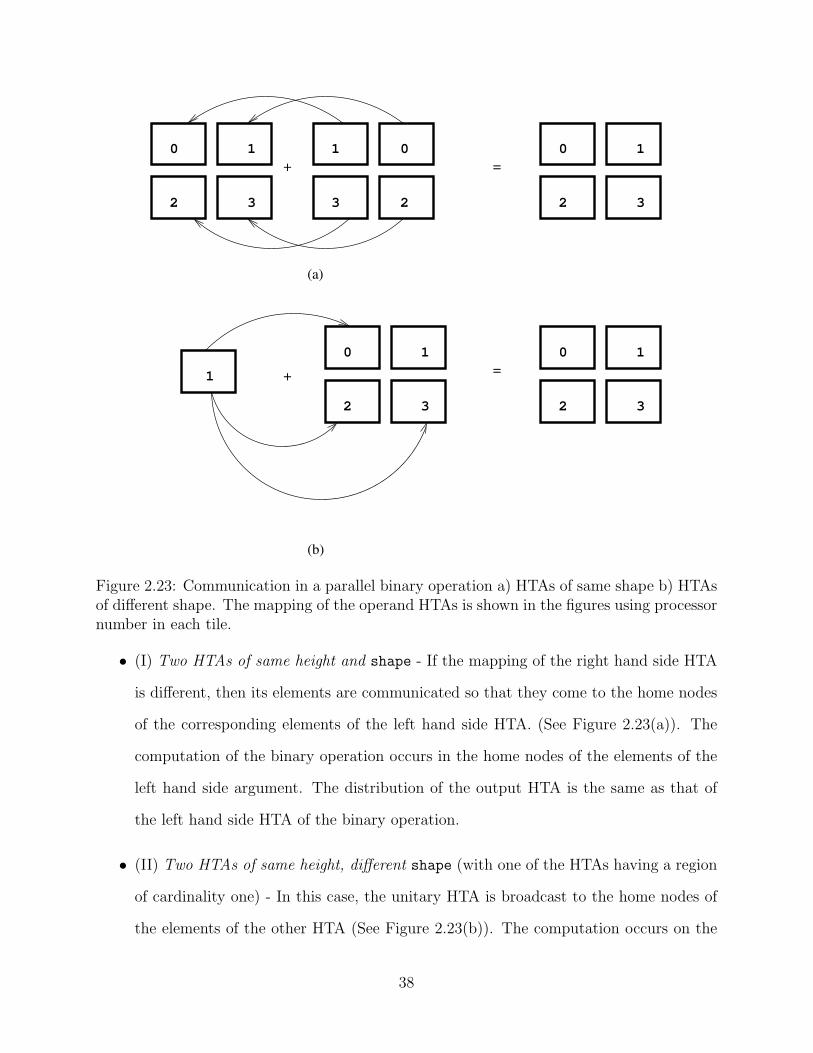
3 2
1 0
(a)
(b)
2 3
0 1
2 3
0 1
2 3
0 1
2 3
0 1
=
=1
+
+
Figure 2.23: Communication in a parallel binary operation a) HTAs of same shape b) HTAsof different shape. The mapping of the operand HTAs is shown in the figures using processornumber in each tile.
• (I) Two HTAs of same height and shape - If the mapping of the right hand side HTA
is different, then its elements are communicated so that they come to the home nodes
of the corresponding elements of the left hand side HTA. (See Figure 2.23(a)). The
computation of the binary operation occurs in the home nodes of the elements of the
left hand side argument. The distribution of the output HTA is the same as that of
the left hand side HTA of the binary operation.
• (II) Two HTAs of same height, different shape (with one of the HTAs having a region
of cardinality one) - In this case, the unitary HTA is broadcast to the home nodes of
the elements of the other HTA (See Figure 2.23(b)). The computation occurs on the
38

0 1
2 3
= + + +
2 3
1 0
3 2
0 1 3 2
0 1
1 3
2 0
Figure 2.24: A chain of binary expression with HTAs of different processor mapping
home nodes of the elements of the larger HTA. The distribution of the output HTA is
same as that of the larger HTA.
• (III) Two HTAs of different height, hl and vm, with l > m. The semantics is the same
as that of (II), with the HTA of lesser height being treated as the unitary HTA (i.e.,
one with region of cardinality one). The computation occurs on the home nodes of the
elements of the higher level HTA. The distribution of the output HTA is same as that
of the higher level HTA.
The above semantics of binary operations may lead to suboptimal communication.
Consider a chain of binary expression (A = B + C + D + E). If all A, B, C, D and
E are of different mapping as shown in Figure 2.24, evaluation of each of the sub-
expression and the final assignment leads to communication. A potential optimization
is to evaluate the entire statement (including the assignment) as a whole operation.
Evaluating it as a whole operation will provide the ability to analyze the expression
tree and reduce the communication. For example, we can choose the node of operation
to be always the LHS operand or the best choice that leads to optimal communication
or perform tree height reduction.
2.3.4 HTA access operation
• Single element selection : Accessing a single element of an HTA hl returns an
HTA, rl−1. If the level l−1 of h is also distributed, distribution of r remains the same.
If it is not distributed, then r is an HTA which is stored only in the home node of the
tile selected.
39

• Selecting a region of elements : Accessing a region of elements of an HTA hl
results in an HTA of same height (l). The distribution of the HTA is a sub-distribution
of h, formed according to the region specified in the access operation.
• Chaining of access operations : Accessing an element or a region of scalars
through chaining (i.e., for example, h(r0, r1)[:, :]) leads to data-parallel access of
the elements, where in the the home nodes that belong to the region (r0, r1), select the
elements.
• Flattening : Flattening (i.e h[:,:]), leads to all-to-all exchange of the values among the
home nodes of the elements of h. The result array is replicated in all the processors.
2.3.5 Assignments
For parallel execution, there are two kinds of assignments = and ←. The semantics of =
is same as that of the assignment operation described earlier in Section 2.2.3. In addition
to that, during an HTA assignment, A = B, if A and B have different processor mapping,
the elements from B are communicated to those of A. The home nodes of the elements of A
wait until they receive the message from the home nodes of the elements of B.
Assignment A← B is split-phase assignment [23]. Two← assignment statements S1 and
S2 can be allowed to be executed concurrently as opposed to the strict sequential order of
execution imposed by the other HTA operations, including =. During a ← assignment, the
home nodes of the elements of A and B need not wait for assignment operation to complete.
The statement A ← B merely initiates the data transfer. An sync statement should be
explicitly invoked at a later point to finish the operation. Several, non-aliasing (i.e., with
no aliasing of memory of the participating HTAs) asynchronous assignment statements can
be in-progress simultaneously until a sync statement is reached. All the statements that
are in-progress (i.e., whose sync point is not reached) are said be in the same phase. If the
assignment statements in a given phase have aliases, then the result is un-defined. Also,
40
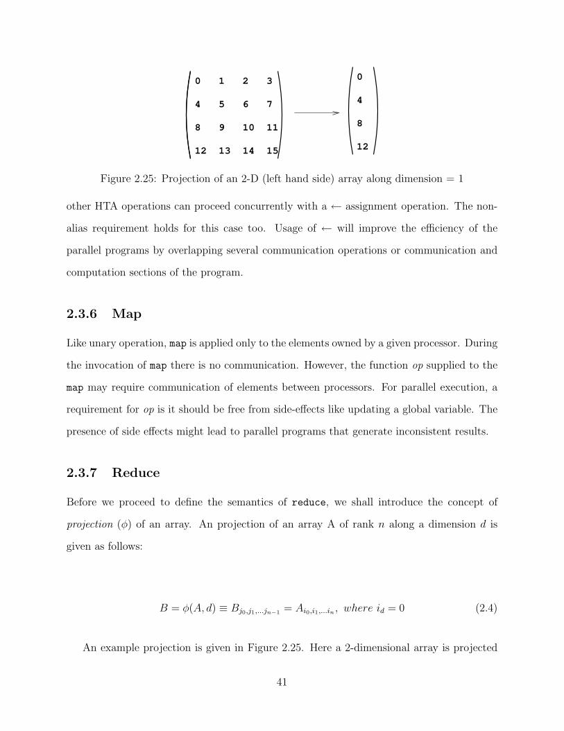
0
4
8
12
0 1 2 3
4 5 6 7
8 9 10 11
12 13 14 15
Figure 2.25: Projection of an 2-D (left hand side) array along dimension = 1
other HTA operations can proceed concurrently with a ← assignment operation. The non-
alias requirement holds for this case too. Usage of ← will improve the efficiency of the
parallel programs by overlapping several communication operations or communication and
computation sections of the program.
2.3.6 Map
Like unary operation, map is applied only to the elements owned by a given processor. During
the invocation of map there is no communication. However, the function op supplied to the
map may require communication of elements between processors. For parallel execution, a
requirement for op is it should be free from side-effects like updating a global variable. The
presence of side effects might lead to parallel programs that generate inconsistent results.
2.3.7 Reduce
Before we proceed to define the semantics of reduce, we shall introduce the concept of
projection (φ) of an array. An projection of an array A of rank n along a dimension d is
given as follows:
B = φ(A, d) ≡ Bj0,j1,...jn−1 = Ai0,i1,...in , where id = 0 (2.4)
An example projection is given in Figure 2.25. Here a 2-dimensional array is projected
41

2
0
2 3
0 1
Figure 2.26: Communication in a partial reduce operation along dim=1, without replica-tion. The left hand side sub-figures describes the distribution of input HTA, the right handside sub-figure describes the distribution of output HTA
along dimension one (i.e., along the columns). The result is the first column of the original
array.
The semantics of parallel reduce depends on the parameters of reduce.
• Case (i) : For the reduce of the kind reduce (op) (i.e., full reduction along all the
dimensions), the result is a scalar that is replicated in all the processors.
• Case (ii): For the reduce of the kind reduce (op, dim) (i.e., partial reduction along a
dimension), the distribution of the resulting HTA is the projection of the distribution
of the original HTA along the dimension dim (see Figure 2.26). The communication be-
tween processors depends on the algorithm used to implement reduction. For example,
if a hyper-cube algorithm is used, then the processors (along the dimension of reduc-
tion) that differ in ith bit of the binary representation of their identifier communicate
during the ith stage of reduction, for a total of log(ddim) stages.
2.3.8 Collective operations
For the HTA reshaping operations, the parallel semantics depends on the kind of operation.
Here, we list the parallel semantics of some of the most frequently used HTA reshaping
operations.
• transpose (Dimension transposition) : A transposition of an HTA h results in the
exchange of elements among the processors. For a square HTA (i.e., HTA whose size
42

2 3
0 1
2 3
0 1
3 4 5
0 1 2
(a)
(b)
0 3
1 4
2 5
0 1
2 3
4 5
Figure 2.27: Communication in a transpose operation a) square HTA b) non-square HTA.In both the figures, the left hand side sub-figures describe the distribution of input HTA, theright hand side sub-figures describe the distribution of the output HTA. In (b) the middlefigure is the transposed distribution of the input HTA
is same along all the dimensions), the processor that owns the tile hi,j (assuming the
HTA is of rank 2) exchanges its tile with the processor that owns the tile hj,i (See
Figure 2.27(a)). For higher dimensional HTAs also, similar rules apply. Even if the
HTA is not a square, but the dimensions to be transposed are of equal size than the
same semantics hold true.
If the dimensions to be transposed are not of equal size, the distribution of the result
HTA is computed using the type of the distribution of the original HTA. For example,
if the original HTA has row-cyclic distribution of elements to processors in row major
43

0
3 4 5
1 2
6 7 8
0
3
6
Figure 2.28: Communication in a repmat operation. In the figure, the left hand side sub-figure describes the distribution of input HTA, the right hand side sub-figure describes thedistribution of output HTA.
order of the elements, the same distribution is applied to the new HTA that results
after the transposition. The exchange of elements is dictated by the transposed (along
the same dimensions as the HTA transposition) original distribution and the new
distribution. (See Figure 2.27(b)). This is the most general semantics of transposition
and covers the earlier semantics of square HTAs also.
• htranspose (Level transposition) : The parallel semantics of htranspose is same as
that of MPI Allgather communication method. That is, each processor sends data to
every other processor. The distribution of the input HTA remains the same after the
operation.
• permute : The distribution of the input HTA is also permuted in the same way as the
HTA. The distribution of the new HTA is computed using the same distribution func-
tion of the input HTA. The communication is dictated by the permuted distribution
of the input HTA and the distribution of the new HTA.
• repmat : For a repmat operation, the distribution of the output HTA is computed using
the same distribution function (dist-type) of the input HTA. The parallel semantics
of the repmat operation is quite different from the rest of the operations discussed
earlier in that the result HTA may be distributed among more number of processors
than the original HTA. This is because, the new HTA typically has more elements
44

than the original HTA. For instance, in the Figure 2.28, the input HTA is distributed
only among three processors (0, 3, 6). The result HTA is distributed on 9 processors.
45
Chapter 3
Implementation
3.1 Introduction
In this chapter we describe the implementation details of the HTA library. Our first imple-
mentation of the HTA library was in MATLAB. MATLAB is a natural choice for HTAs for
several reasons. MATLAB is an object oriented array programming language, with a rich
set of array and vector operations and operator overloading capability. Thus, it is very easy
to extend the operations to HTAs. The use of MATLAB lead to the introduction of new
operations for HTAs. The MATLAB implementation provided the ground for understanding
HTAs and evolving the HTA operations.
However, owing to various limitations, the execution times of MATLAB is usually sig-
nificantly larger than that of FORTRAN77. This motivated the C++ implementation.
C++ [26] is a popular object oriented programming language. Unlike MATLAB, C++ is
a scalar based compiled programming language. Due to its object oriented nature and the
presence of templates, C++ allows easy creation of data structures like HTA. Like MATLAB,
C++ also has operator overloading capability.
The underlying execution model and the semantics of HTA operations remain the same
in both the MATLAB and C++ implementations. Due to the syntactical differences in
the MATLAB and C++ language, few operations are represented differently. The most
important difference between MATLAB and C++ is that the latter uses 0-origin indexing,
while the former using 1-origin indexing. Table 3.1 lists the MATLAB and C++ constructs
for various HTA operations discussed in Chapter 2. At the end of the chapter we provide
46

Table 3.1: MATLAB and C++ syntax for various HTA operations.
HTA Construct MATLAB syntax C++ syntax
tuple (i0, i1, ..in−1) T (i0, i1, ..in−1)range low[: stride] : high R(low, high[, stride])region (l1[: s1] : h1, l2[: s2] : h2) (R(l1, h1[, s1]), R(l2, h2[, s2]))
() {} ()[] () []= = =← N/A async{...}sync
+,-,*,/ +, -, *, / +, -, /transpose(h) ’ h.transpose()permute(h) permute (h, perm vector) h.permute(perm vector)
replicate(h) repmat (h, rep vector) h.repmat(rep vector)map(h) feval (@func, h,...) h.map(op,..)
reduce(h) reduce (@func, h...) h.reduce(op,...)scan(h) scan (@func, h...) h.scan(op,...)
several simple HTA programs, for which we will use the specific operators described in the
Table 3.1, rather than the abstract operator discussed in the preceding chapter.
3.2 Execution Model of HTA programs
The programing model of HTA programs differs from the SPMD-style programming, where
programmers have to specify the program execution path for each processor and have to
explicitly synchronize the processors. Instead, HTA programs offer global view of data with
single threaded execution. All the processors execute the same program. Global scalar
variables, arrays and non-distributed HTAs are replicated in each processor, so that every
copy keeps the same value. Distributed HTAs are also created in every processor, including
those ones that do not own tiles of the HTA, which will only keep information about the
structure of the HTA.
When a expression involving one or more HTAs is evaluated, each processor applies
locally the operation of the expression on the tiles of the HTA it owns. In the case of
binary operations, the processors check the location of the corresponding tiles that need to
be operated. Those tiles of the right operand that are not located in the processor that owns
the associated tile of the left operand, are sent to that processor. The processors that own
the tiles of the left HTA perform the desired operation and store the resulting tiles.
Similar execution happens when the right hand side (RHS) of an assignment is not
47

(1) a{1,1} = mtrx;(2) b{:,:} = a{1,1};
Figure 3.1: Simple code example
mapped to the mesh of processors in the same way as the left hand side (LHS). Every tile
of the RHS HTA of the assignment is sent to the processor that owns the corresponding tile
of the LHS HTA to which it is assigned.
Figure 3.1 shows an example code snippet written in our MATLAB implementation.
Here, we assume that a and b are 2 × 2 HTAs and distributed in row-cyclic fashion.
For simplicity in foregoing discussion, we refer to the home node of a tile as (i,j), where
(i,j)∈ {(1, 1), (1, 0), (2, 1), (2, 2)}. During the assignment statement, the matrix mtrx is
assigned to a{1,1} in processor (1,1). The other processors also execute this statement,
but since it applies to a tile that they do not own, they do nothing and wait for the next
method invocation.
The next statement involves an access operation. This statement returns a HTA of level
0 and size 1× 1 (i.e., a singe tile). This tile resides in only one processor, the owner of tile
(1,1). Selection is followed by assignment of the result to all the tiles of b. This involves a
broadcast of the left hand side to all the processors.
Explicit synchronization between processors is not necessary. For our run time library,
we used two-sided communication model where in, the synchronization is always implicit
because communication takes place from the producer to the consumer, so an eager consumer
always has to wait for a delayed producer to send the data before it can proceed with the
computation. As a result, computation and/or communication can be overlapped even
between different statements. It is also possible to execute two statements concurrently,
without affecting the sequential deterministic semantics.
Consider the example in Figure 3.2-(a), where a is a 2 × 2 HTA distributed using
row-cyclic distribution. and mtrx1 and mtrx2 are two matrices. The MATLAB inter-
preter calls the overloaded assignment method of the HTA class in all the processors for
48

(1) a{1:2, 1} = mtrx1;
(2) a{1:2, 2} = mtrx2;
(a)
a{2,1} = mtrx1
φ
φ
φ
φ a{2,2} = mtrx1
(1,1)
(1,2)
(2,2)
(2,1)
a{1,2} = mtrx1
a{1,1} = mtrx1
ProcessorTime
(b)
Figure 3.2: (a) Example of code with concurrent execution. (b) Timeline for the processorsexecuting the code in (a).
statement (1). Only processors (1,1) and (2,1) are involved in this assignment, so they ex-
ecute it, while processors (1,2) and (2,2) exit the assignment operation right after checking
the ownership. The MATLAB interpreter will then invoke the HTA assignment method
in processors (1,2) and (2,2) for the statement (2), and since they own the tiles involved
in this second assignment, they will perform it. The MATLAB interpreter will invoke the
assignment method in processors (1,1) and (2,1) later, since they were assigning mtrx1 to
their tiles. In this second statement, processors (1,1) and (2,1) do not own the involved tiles,
so they will exit the method right after they check ownership. Figure 3.2 shows how the
execution time of the statement (1) in processors (1,1) and (2,1) is overlapped with that of
the statement (2) in processors (1,2) and (2,2). The letter φ denotes the time used by a
processor to check that an instruction does not affect the tiles it owns.
3.3 Underlying Implementation
Although the SPMD-programming style is usually more difficult for programmers, it is very
efficient with respect to performance. For these reasons, the underlying run time HTA library
follows the SPMD approach. As mentioned earlier each processor executes the same program
and hence every statement is executed by the processors. The program is linked with the run
time library in each node of a cluster. The run time library governs the execution for a given
processor depending on the processor mapping of the HTAs involved in a given statement.
49

MATLAB
HTA toolbox
MATLAB
HTA toolbox
1 32 4
1 32 4
MATLAB
HTA toolbox
1 32 4
MATLAB
HTA toolbox
1 32 4
1 32 4
Figure 3.3: HTA implementation.
If the HTA method finds the processor it is running on does not have any data participating
in the HTA method or operation, it exits.
Figure 3.3 shows an high level view of the underlying execution. Each node has an
instance of MATLAB, the HTA library and the MATLAB+HTA program. They com-
municate among themselves when required. Communication is performed using the MPI
library. The communication is performed transparently to the programmer without his in-
tervention. Communication is performed by either MPI Send/MPI Recv or MPI AlltoAll
or MPI Reduce and their variants. The library also uses non-blocking MPI ISend and
MPI IRecv for point-to-point exchanges, when necessary. For some operations, collective
communication routines of the MPI are used. For example, the transpose operation is
implemented using MPI AlltoAll routine. The reduce operations are implemented using
50
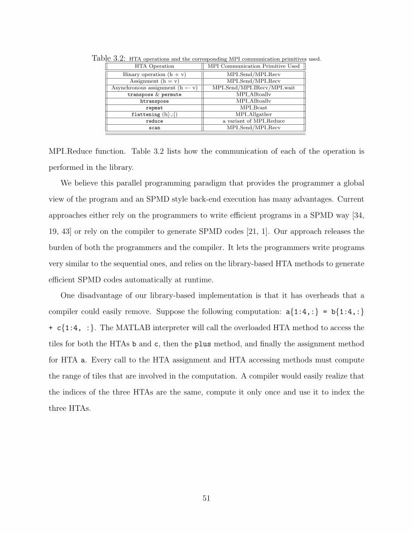
Table 3.2: HTA operations and the corresponding MPI communication primitives used.
HTA Operation MPI Communication Primitive Used
Binary operation (h + v) MPI Send/MPI RecvAssignment (h = v) MPI Send/MPI Recv
Asynchronous assignment (h ← v) MPI Send/MPI IRecv/MPI waittranspose & permute MPI Alltoallv
htranspose MPI Alltoallvrepmat MPI Bcast
flattening (h[:,:]) MPI Allgatherreduce a variant of MPI Reducescan MPI Send/MPI Recv
MPI Reduce function. Table 3.2 lists how the communication of each of the operation is
performed in the library.
We believe this parallel programming paradigm that provides the programmer a global
view of the program and an SPMD style back-end execution has many advantages. Current
approaches either rely on the programmers to write efficient programs in a SPMD way [34,
19, 43] or rely on the compiler to generate SPMD codes [21, 1]. Our approach releases the
burden of both the programmers and the compiler. It lets the programmers write programs
very similar to the sequential ones, and relies on the library-based HTA methods to generate
efficient SPMD codes automatically at runtime.
One disadvantage of our library-based implementation is that it has overheads that a
compiler could easily remove. Suppose the following computation: a{1:4,:} = b{1:4,:}
+ c{1:4, :}. The MATLAB interpreter will call the overloaded HTA method to access the
tiles for both the HTAs b and c, then the plus method, and finally the assignment method
for HTA a. Every call to the HTA assignment and HTA accessing methods must compute
the range of tiles that are involved in the computation. A compiler would easily realize that
the indices of the three HTAs are the same, compute it only once and use it to index the
three HTAs.
51
3.4 MATLAB Library
3.4.1 The HTA class data type
The MATLAB implementation of HTA is based on cell arrays. Cell arrays in MATLAB are
multidimensional arrays whose elements are copies of other arrays. A cell array of empty
matrices can be created with the cell function. But, more often, cell arrays are created by
enclosing a miscellaneous collection of things in curly braces, ‘{}’. The curly braces are also
used with subscripts to access the contents of various cells. Cell arrays can be used to store
sequences of matrices of different sizes.
The HTA class in MATLAB contains a cell array as its primary field. The other impor-
tant fields of the class are size, dimensions and the arrangement of processors. MATLAB
provides two access operators - ’{}’ and ’()’. The former is to access cell arrays and the
latter for normal arrays. We overloaded these two operators for the HTA class to use them
for tile access and scalar access respectively. These two methods are also known as subsref
methods. The assignment operator in MATLAB is known as subsasgn. This is also over-
loaded for the HTA class. Apart from them, all the primitive unary and binary operations
are also overloaded.
The constructor of the class, hta, is used by the programmer to construct HTAs. Both
top down and bottom–up constructors are implemented. For example, the HTA of the
Figure 2.1(a) of Chapter 2 could be created using a source matrix MX and the bottom–up
HTA constructor, as follows:
A = hta(MX, {1:2:10,1:3:12});
The HTAs built above are local. In order to request the distribution of the top-level tiles
of the HTA on a mesh of processors, the last argument of the constructor must be a vector
specifying processor mapping or dist-type. The default distribution is currently fixed to
52

be row-cyclic.
HTAs can also be built as structures whose tiles are empty using top–down constructor.
In this case the top-down constructor is called just with the number of tiles desired in each
dimension. The empty tiles can be filled in later by means of assignments. As an, example,
the following statement generates an empty 4×4 HTA whose tiles are distributed on a 2×2
processor mesh. The assignment statement that follows the construction, initializes the tiles
of the HTA A to contain an array of ones of size 2× 3.
A = hta(5, 4);
A{:,:} = ones(2,3);
3.4.2 Interfacing with MPI and Other implementation details
MATLAB provides a mechanism to call functions written in C to be invoked from the
MATLAB environment. These functions are stand alone functions and are compiled with
the MEX compiler provided by the MATLAB distribution. The variables from the MATLAB
environment can be passed in to these functions, and can be modified within them. We use
this facility to interface with the MPI library. All the communication operations are written
in C and they in turn call the MPI library routines. Small methods used very frequently are
also written in C for performance reasons.
Our framework requires that all the processors participating in the system have a copy
of MATLAB and the HTA toolbox. This imposed a serious practical limitation. Running
on large number of processors requires equally large number of MATLAB licenses.
We have written two versions of our HTA class. One of them checks the legality of
every operation performed on an HTA and provides error messages when any problem is
detected. For example, it checks that the indices used when dereferencing an HTA are inside
the dimensions of the HTA, or it checks that two HTAs are conformable before applying
a binary operation to them. This implementation is meant to help find problems in the
53

programs at the cost of extra overheads. The second version, with no checks, can be used
when the programmer feels his/her code is reliable enough and seeks more performance.
Our implementation follows the copy-on-write behavior of MATLABTM. In MATLABTM,
an assignment to a variable implies simply the creation of a pointer or reference to the
assigned value. This way, several variables may be pointing to the same data. When an
assignment through one of these variables tries to modify parts of this data, MATLABTM
builds a private copy of the data for that variable and applies the requested changes. While
this is a reasonable strategy, sometimes unneeded copies are made because MATLABTM
only allows pass by value of variables to its functions.
Following an assignment, the RHS is not actually copied, but rather a reference is created
from the LHS of the assignment to the old value. A copy is only made when the user attempts
to modify the data referred to. Since our HTAs are implemented with the same variables that
MATLABTM uses, an HTA can have multiple references to it. Private copies of distributed
HTAs are made only when they have several handles/names in the program and some of
them tries to modify the contents of the HTA.
3.4.3 Run time overheads
MATLAB is an interpreted and interactive programming language. This makes it easy to
debug MATLAB programs. Another advantage is its operator overloading capability, using
which we have overloaded several common operations that have very natural meaning. More-
over, MATLAB has garbage collection which eliminates the need for tedious allocation/de-
allocation statements to be inserted by the programmers.
The fusion of HTAs with MATLAB lead to very clear parallel programs. However,
MATLAB programs are slow and suffer from several run time overheads. Owing to its
interpreted, nature only vectorized instructions deliver optimal performance. Loops that
cannot be vectorized typically result in a significant slowdown. Examples of programs that
exhibit this behavior are the LU and BT of the NAS benchmark suite. These programs have
54

global data dependencies arising from linear recurrences that cannot be easily vectorized.
Even if all the computations are vectorized, other MATLAB overheads restrict the pro-
grams’ performance. One source of error is the creation of temporary arrays while evaluating
a chain of expressions. In addition, MATLAB used copy-on-write policy. Though, this copy
is performed lazily on a write, they could potentially degrade the performance of MATLAB
programs.
3.5 C++
3.5.1 Overview
C++ library is based on templates and object oriented features of C++. We refer to the
C++ library as htalib. In htalib, the HTAs are implemented using various templated classes.
The classes can be broadly classified in to two categories - front-end and back-end.
The front end classes are those that are exposed to the programmer. They provide
an uniform interface for all the kinds of HTAs (i.e., distributed,shared, serial, sparse etc)
and delegate the HTA operations to the respective back-end classes. Apart from this, they
also perform the automatic memory management of the HTAs using a simple reference
counting based garbage collection scheme. Consequently, the instances of the HTAs cannot
be allocated on heap section of the address space.
The back end classes implements all the HTA operations, including the communication.
These classes in turn uses libraries like MPI for specific tasks.
3.5.2 Front End classes
The core classes of the front end fall into four categories:
Logical index space. Classes used to define index space and tiling of an HTA are
Tuple<N>, an N-dimensional index value from Zn; Triplet, a 1-dimensional range with
55
optional stride (low:high[:step]); and Region<N>, an N-dimensional rectangular index
space spanned by N triplets. Region also provides an iterator to iterate over each of the
individual index points. Instances of Tuple<N>, Triplet and Region are values, i.e., once
defined, their value cannot change.
HTA. Class HTA<T,N> defines an HTA with scalar elements of type T and N dimen-
sions. The data type provides the interface for scalar access (operator[]), tile access
(operator()), point-wise operations, transpose, permute, dpermute, map and reduce that
are described in chapter 2. An HTA is part of a hierarchical structure of recursively composed
HTAs.
Machine mapping. The machine mapping of an HTA specifies (i) where the HTA is allo-
cated in a distributed system and (ii) the memory layout of the scalar data array underlying
the HTA. The former aspect is captured by instances of class Distribution that specifies
the home location of the scalar data for each of the tiles of an HTA. The latter aspect is
represented by instances of class MemoryMapping that specify the layout (row-major across
tiles, row-major per tile etc.), size and stride of the flat array data underlying the HTA.
The machine mapping is accessed internally by the htalib, for example, to orchestrate im-
plicit communication. The machine mapping is also available through the API of the library
to facilitate direct access and communication of array data in case the programmer intends
to bypass the access mechanisms provided by HTAs. In the current implementation, the
complete information about the machine mapping is available in each node of a distributed
system.
3.5.3 Back End classes
The complete class hierarchy of the back end classes is shown in the Figure 3.4. In the
Figure 3.4, AbstractArray<T, N> is an abstract base class, while Array<T, N> is its sub-
class. Array<T, N> is also a reference counted class. That is, all its instances in the heap
56
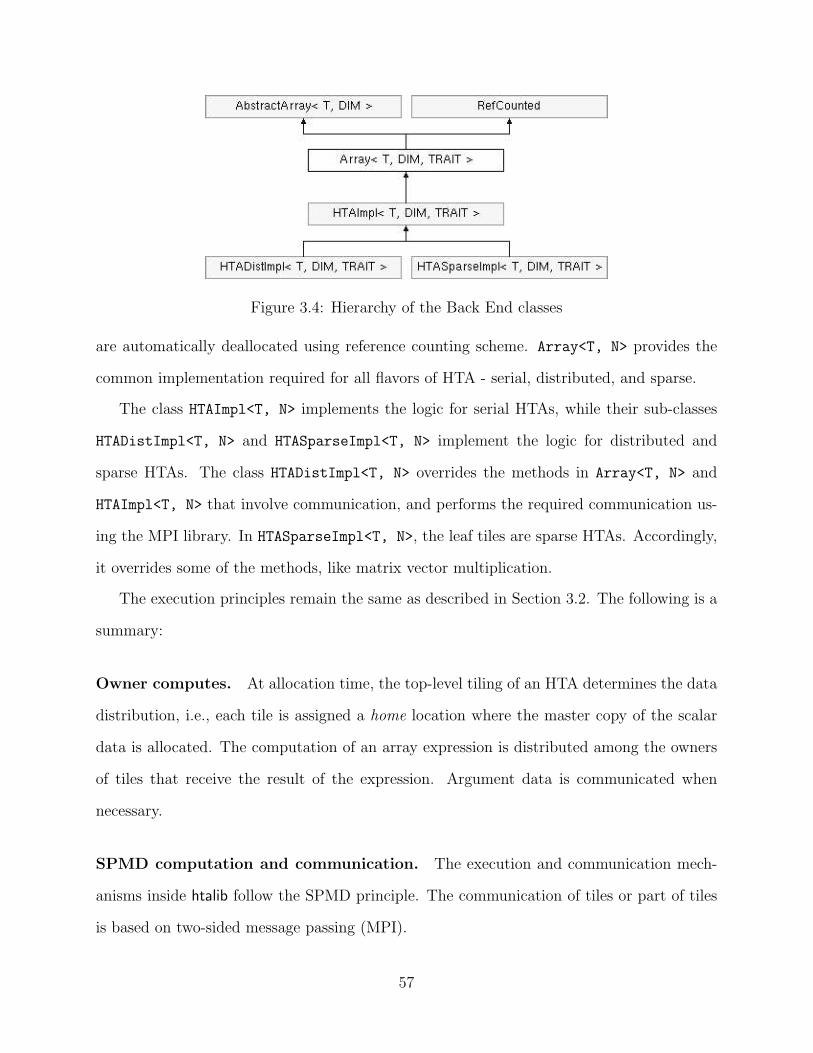
Figure 3.4: Hierarchy of the Back End classes
are automatically deallocated using reference counting scheme. Array<T, N> provides the
common implementation required for all flavors of HTA - serial, distributed, and sparse.
The class HTAImpl<T, N> implements the logic for serial HTAs, while their sub-classes
HTADistImpl<T, N> and HTASparseImpl<T, N> implement the logic for distributed and
sparse HTAs. The class HTADistImpl<T, N> overrides the methods in Array<T, N> and
HTAImpl<T, N> that involve communication, and performs the required communication us-
ing the MPI library. In HTASparseImpl<T, N>, the leaf tiles are sparse HTAs. Accordingly,
it overrides some of the methods, like matrix vector multiplication.
The execution principles remain the same as described in Section 3.2. The following is a
summary:
Owner computes. At allocation time, the top-level tiling of an HTA determines the data
distribution, i.e., each tile is assigned a home location where the master copy of the scalar
data is allocated. The computation of an array expression is distributed among the owners
of tiles that receive the result of the expression. Argument data is communicated when
necessary.
SPMD computation and communication. The execution and communication mech-
anisms inside htalib follow the SPMD principle. The communication of tiles or part of tiles
is based on two-sided message passing (MPI).
57

htalib::async();
B(1:n)[0] = B(0:n-1)[d];
B(0:n-1)[d+1] = B(1:n)[1];
htalib::sync();
Figure 3.5: Relaxing sequential evaluation order to facilitate overlap of communication andcomputation.
Apart from the data distribution aspect, a programmer is not concerned with this model
(global view, cf. Section 3.2). The implementation of htalib is flexible to accommodate other
communication platforms also. We also have an experimental UPC-based shared memory
runtime system [10] as communication platform.
3.5.4 Performance Optimizations
Unlike MATLAB, the C++ library offers more freedom in performing certain optimizations.
Following are some of the optimizations that we implemented in the C++ library.
Dynamic optimizations. htalib implements lazy evaluation to reduce or avoid the over-
head due to temporary arrays. At an array assignment, the evaluation of the rhs is delayed
until the target of the assignment is determined. If lhs and rhs have no data dependence,
the assignment is directly evaluated into the lhs.
The second optimization is the reuse of HTAs that hold intermediate results of array ex-
pressions. htalib maintains internally a pool of HTAs that take the role of ’registers’. During
the evaluation of an array expression, ’HTA registers’ with matching tiling are allocated and
recycled in the pool.
Relaxation of serial evaluation semantics. htalib provides a mechanism to temporarily
relax the serial evaluation ordering and overlap of communication with computation. The
example in Figure 3.5 shows the boundary exchange in the C++ version of the Jacobi
example of Figure 3.6.2(a). As there is no data dependence among the assignments, both
statements can proceed concurrently. This is achieved through the runtime calls to asyc and
sync. All the assignment statements between async and sync are interpreted by the library
58
to be ← and resort to split-phase semantics [23]. We earlier described this asynchronous
assignment (←) in Chapter 2.
3.6 Examples
In this section we will illustrate several simple examples of HTA programs. These programs
are well known numerical programs. Specifically, we will look at two algorithms - matrix
matrix multiplication and stencil computation. We consider two parallel matrix matrix mul-
tiplication, namely, cannon and summa matrix multiplication. We also include an example
of recursive matrix matrix multiplication.
3.6.1 Matrix Multiplication
This section describes HTA programs for multiplying two (n, n) dense, square matrices A and
B to yield the product matrix C = A× B. All the programs are based on the conventional
serial matrix multiplication algorithm shown in the Algorithm 4. In the following algorithms
we use the operation .× to mean scalar multiplication, while × for matrix multiplication.
Though, × can be used for multiplying two scalars as well, we do not use it to avoid confusion
when we want to perform a scalar multiplication over each scalar elements of two matrices.
Before proceeding to the parallel version of the matrix multiplication, we introduce the
concept of block matrix operations. We can express the matrix multiplication algorithm
in terms of block matrix operations as shown in Algorithm 5. A (n, n) matrix A can be
regarded as a (q, q) array of blocks Ai,j(0 ≤ i, j < q) such that each block is an ((n/q), (n/q))
sub-matrix. The scalar assignment, multiplication and addition operations in Algorithm 4
are replaced with matrix multiplication and matrix addition respectively. Both the scalar
and the blocked versions of the matrix multiplication have the same run time complexity of
O(n3).
59

function C = matmul (A, B, C)
if (level(A) == LEAF_LEVEL)
C = C + A * B;
else
for i=1:size(A,1)
for k=1:size(A,2)
for j=1:size(B,2)
C{i, j} = matmul(A{i,k}, B{k,j}, C{i,j});
end
end
end
end
Figure 3.6: Recursive matrix-matrix multiplication that exploits cache locality.
Recursive Blocked Matrix Matrix Multiplication using HTAs
Algorithm 4 MAT MULT
1: A, B and C are matrices of scalar values.2: for i = 0 to n− 1 do3: for j = 0 to n− 1 do4: C[i, j] := 05: for k = 0 to n− 1 do6: C[i, j] := C[i,j] + A[i,k] .× B[k,j]7: end for8: end for9: end for
Algorithm 5 BLOCK MAT MULT
1: A, B, and C are matrices of blocks; each block is of size n/q × n/q2: for i = 0 to q − 1 do3: for j = 0 to q − 1 do4: C[i, j] := 05: for k = 0 to q − 1 do6: C[i, j] := C[i,j] + A[i,k] × B[k,j]7: end for8: end for9: end for
Blocked versions of matrix multiplication are more efficient on processors with cache
due to the benefits from the locality of reference. Typically, such programs are written
using techniques known as as loop tiling or loop blocking [50]. Generally, a programmer
(or a compiler) tiles a loop nest of depth n by modifying the bounds of the original loops
and introducing n extra loops. These extra loops control the iteration over tiles, while the
modified original loops iterate over the scalar elements.
60

Using HTA, such tiled computation can be expressed naturally and easily. The tiled
matrix-matrix multiplication matmul of Figure 3.6 is an example of a tiled computation. If
A is not a scalar or a matrix, we have to recursively proceed down into the HTA hierarchy
until we reach the leaf tile of the HTA.
SUMMA Algorithm
Algorithm 6 MATMUL OUTER PRODUCT
1: for k = 0 to n− 1 do2: C := C + A[:, k] × B[k, :]3: end for
Algorithm 7 SUMMA PARALLEL
1: for k = 0 to n− 1 do2: t1 ← broadcast A[i, k] along row i3: t2 ← broadcast B[k, j] along column j4: C := C + t1 .× t25: end for
Algorithm 8 SUMMA BLOCK PARALLEL
1: A, B, C are matrices of blocks; each block is of size n/q × n/q2: for k = 0 to q − 1 do3: t1 ← broadcast A[i, k] along row i4: t2 ← broadcast B[k, j] along column j5: C := C + t1 × t26: end for
The parallel version of matrix multiplication are also based on the blocked matrix matrix
multiplication.
In the following algorithms, we consider the following decomposition. Two (n, n) matrices
A and B are partitioned in to p blocks Ai,j and Bi,j of size ((n/√
p), (n/√
p)) each. These
blocks are mapped onto a (√
p,√
p) logical mesh of processors. The processors are labeled
from P0,0 to P√(p)−1,
√(p)−1
.
The first algorithm that we describe is the Scalable Universal Matrix Matrix Algorithm
(SUMMA) [31]. SUMMA is based on the outer product version of matrix matrix multipli-
cation, where in the matrix multiplication is realized as a series of rank one updates (See
61
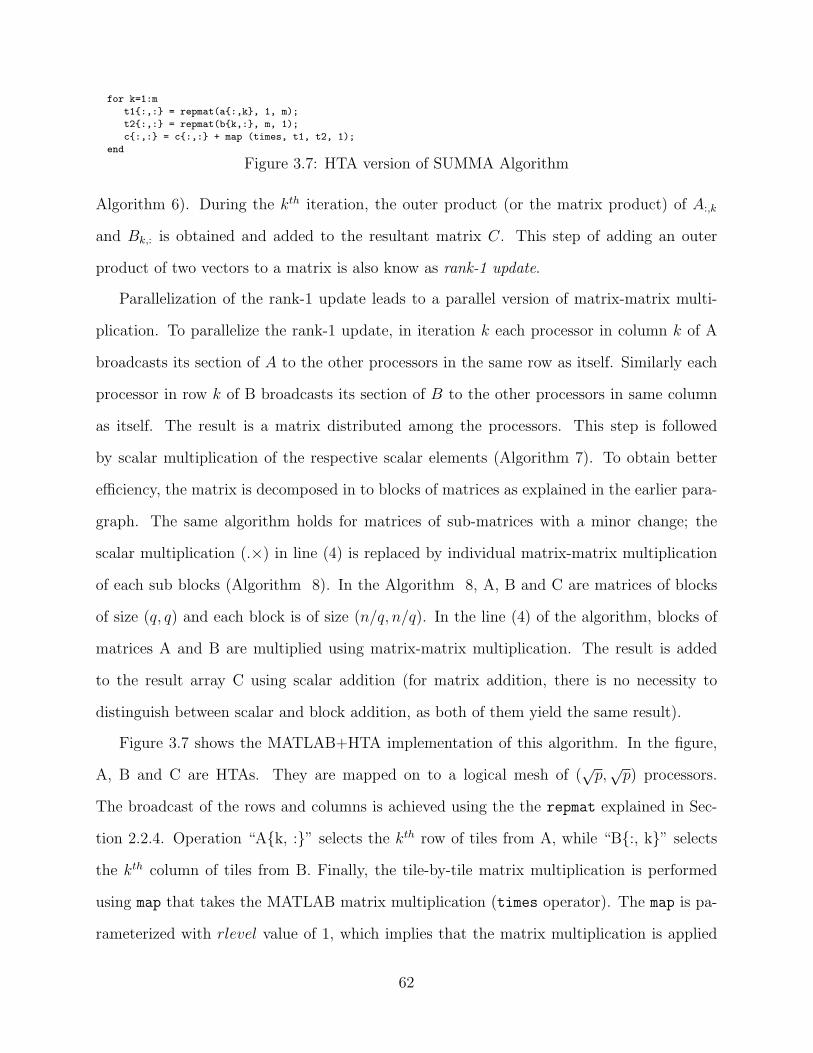
for k=1:m
t1{:,:} = repmat(a{:,k}, 1, m);
t2{:,:} = repmat(b{k,:}, m, 1);
c{:,:} = c{:,:} + map (times, t1, t2, 1);
end
Figure 3.7: HTA version of SUMMA Algorithm
Algorithm 6). During the kth iteration, the outer product (or the matrix product) of A:,k
and Bk,: is obtained and added to the resultant matrix C. This step of adding an outer
product of two vectors to a matrix is also know as rank-1 update.
Parallelization of the rank-1 update leads to a parallel version of matrix-matrix multi-
plication. To parallelize the rank-1 update, in iteration k each processor in column k of A
broadcasts its section of A to the other processors in the same row as itself. Similarly each
processor in row k of B broadcasts its section of B to the other processors in same column
as itself. The result is a matrix distributed among the processors. This step is followed
by scalar multiplication of the respective scalar elements (Algorithm 7). To obtain better
efficiency, the matrix is decomposed in to blocks of matrices as explained in the earlier para-
graph. The same algorithm holds for matrices of sub-matrices with a minor change; the
scalar multiplication (.×) in line (4) is replaced by individual matrix-matrix multiplication
of each sub blocks (Algorithm 8). In the Algorithm 8, A, B and C are matrices of blocks
of size (q, q) and each block is of size (n/q, n/q). In the line (4) of the algorithm, blocks of
matrices A and B are multiplied using matrix-matrix multiplication. The result is added
to the result array C using scalar addition (for matrix addition, there is no necessity to
distinguish between scalar and block addition, as both of them yield the same result).
Figure 3.7 shows the MATLAB+HTA implementation of this algorithm. In the figure,
A, B and C are HTAs. They are mapped on to a logical mesh of (√
p,√
p) processors.
The broadcast of the rows and columns is achieved using the the repmat explained in Sec-
tion 2.2.4. Operation “A{k, :}” selects the kth row of tiles from A, while “B{:, k}” selects
the kth column of tiles from B. Finally, the tile-by-tile matrix multiplication is performed
using map that takes the MATLAB matrix multiplication (times operator). The map is pa-
rameterized with rlevel value of 1, which implies that the matrix multiplication is applied
62
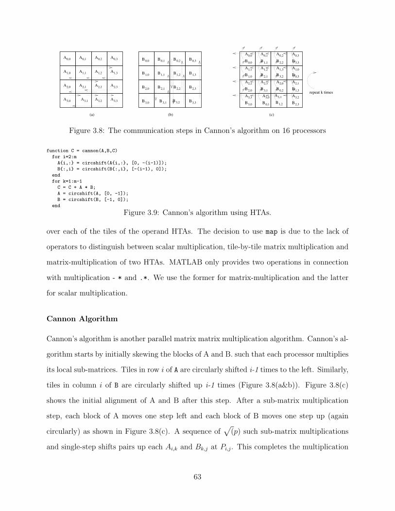
B3,2
B0,2 B0,3
B1,0 B1,1 B1,2 B1,3
B2,0
B3,0
B2,1 B2,2 B2,3
B3,3B3,1
B0,1B0,0
A3,1
(a) (b) (c)
A3,2
A0,2 A0,3
A1,0 A1,1 A1,2 A1,3
A2,0
A3,0
A2,1 A2,2 A2,3
A3,3A3,1
A0,1A0,0
B1,2
B2,2 B3,3
B1,0 B2,1 B3,2 B0,3
B2,0
B3,0
B3,1 B0,2 B1,3
B2,3B0,1
B1,1B0,0
A0,2 A0,3
A1,1 A1,2 A1,3 A1,0
A2,2
A3,3
A2,3 A2,0 A2,1
A3,2A3,0
A0,1A0,0
repeat k times
Figure 3.8: The communication steps in Cannon’s algorithm on 16 processors
function C = cannon(A,B,C)
for i=2:m
A{i,:} = circshift(A{i,:}, [0, -(i-1)]);
B{:,i} = circshift(B{:,i}, [-(i-1), 0]);
end
for k=1:m-1
C = C + A * B;
A = circshift(A, [0, -1]);
B = circshift(B, [-1, 0]);
end
Figure 3.9: Cannon’s algorithm using HTAs.
over each of the tiles of the operand HTAs. The decision to use map is due to the lack of
operators to distinguish between scalar multiplication, tile-by-tile matrix multiplication and
matrix-multiplication of two HTAs. MATLAB only provides two operations in connection
with multiplication - * and .*. We use the former for matrix-multiplication and the latter
for scalar multiplication.
Cannon Algorithm
Cannon’s algorithm is another parallel matrix matrix multiplication algorithm. Cannon’s al-
gorithm starts by initially skewing the blocks of A and B. such that each processor multiplies
its local sub-matrices. Tiles in row i of A are circularly shifted i-1 times to the left. Similarly,
tiles in column i of B are circularly shifted up i-1 times (Figure 3.8(a&b)). Figure 3.8(c)
shows the initial alignment of A and B after this step. After a sub-matrix multiplication
step, each block of A moves one step left and each block of B moves one step up (again
circularly) as shown in Figure 3.8(c). A sequence of√
(p) such sub-matrix multiplications
and single-step shifts pairs up each Ai,k and Bk,j at Pi,j. This completes the multiplication
63
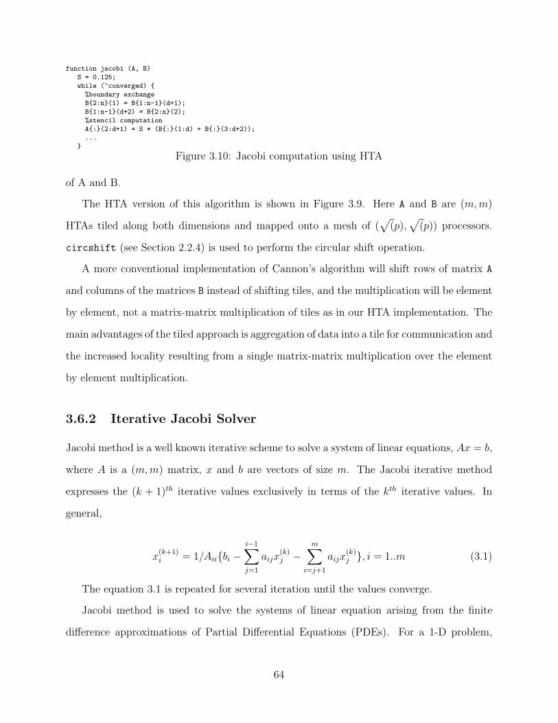
function jacobi (A, B)
S = 0.125;
while (~converged) {
%boundary exchange
B{2:n}(1) = B{1:n-1}(d+1);
B{1:n-1}(d+2) = B{2:n}(2);
%stencil computation
A{:}(2:d+1) = S * (B{:}(1:d) + B{:}(3:d+2));
...
}
Figure 3.10: Jacobi computation using HTA
of A and B.
The HTA version of this algorithm is shown in Figure 3.9. Here A and B are (m, m)
HTAs tiled along both dimensions and mapped onto a mesh of (√
(p),√
(p)) processors.
circshift (see Section 2.2.4) is used to perform the circular shift operation.
A more conventional implementation of Cannon’s algorithm will shift rows of matrix A
and columns of the matrices B instead of shifting tiles, and the multiplication will be element
by element, not a matrix-matrix multiplication of tiles as in our HTA implementation. The
main advantages of the tiled approach is aggregation of data into a tile for communication and
the increased locality resulting from a single matrix-matrix multiplication over the element
by element multiplication.
3.6.2 Iterative Jacobi Solver
Jacobi method is a well known iterative scheme to solve a system of linear equations, Ax = b,
where A is a (m, m) matrix, x and b are vectors of size m. The Jacobi iterative method
expresses the (k + 1)th iterative values exclusively in terms of the kth iterative values. In
general,
x(k+1)i = 1/Aii{bi −
i−1∑j=1
aijx(k)j −
m∑i=j+1
aijx(k)j }, i = 1..m (3.1)
The equation 3.1 is repeated for several iteration until the values converge.
Jacobi method is used to solve the systems of linear equation arising from the finite
difference approximations of Partial Differential Equations (PDEs). For a 1-D problem,
64
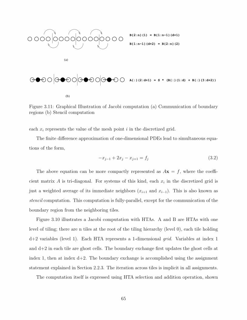
(a)
(b)
B{2:n}(1) = B{1:n−1}(d+1)
B{1:n−1}(d+2) = B{2:n}(2)
A{:}(2:d+1) = S * (B{:}(1:d) + B{:}(3:d+2))
Figure 3.11: Graphical Illustration of Jacobi computation (a) Communication of boundaryregions (b) Stencil computation
each xi represents the value of the mesh point i in the discretized grid.
The finite difference approximation of one-dimensional PDEs lead to simultaneous equa-
tions of the form,
−xj−1 + 2xj − xj+1 = fj (3.2)
The above equation can be more compactly represented as Ax = f , where the coeffi-
cient matrix A is tri-diagonal. For systems of this kind, each xi in the discretized grid is
just a weighted average of its immediate neighbors (xi+1 and xi−1). This is also known as
stencil computation. This computation is fully-parallel, except for the communication of the
boundary region from the neighboring tiles.
Figure 3.10 illustrates a Jacobi computation with HTAs. A and B are HTAs with one
level of tiling; there are n tiles at the root of the tiling hierarchy (level 0), each tile holding
d+2 variables (level 1). Each HTA represents a 1-dimensional grid. Variables at index 1
and d+2 in each tile are ghost cells. The boundary exchange first updates the ghost cells at
index 1, then at index d+2. The boundary exchange is accomplished using the assignment
statement explained in Section 2.2.3. The iteration across tiles is implicit in all assignments.
The computation itself is expressed using HTA selection and addition operation, shown
65
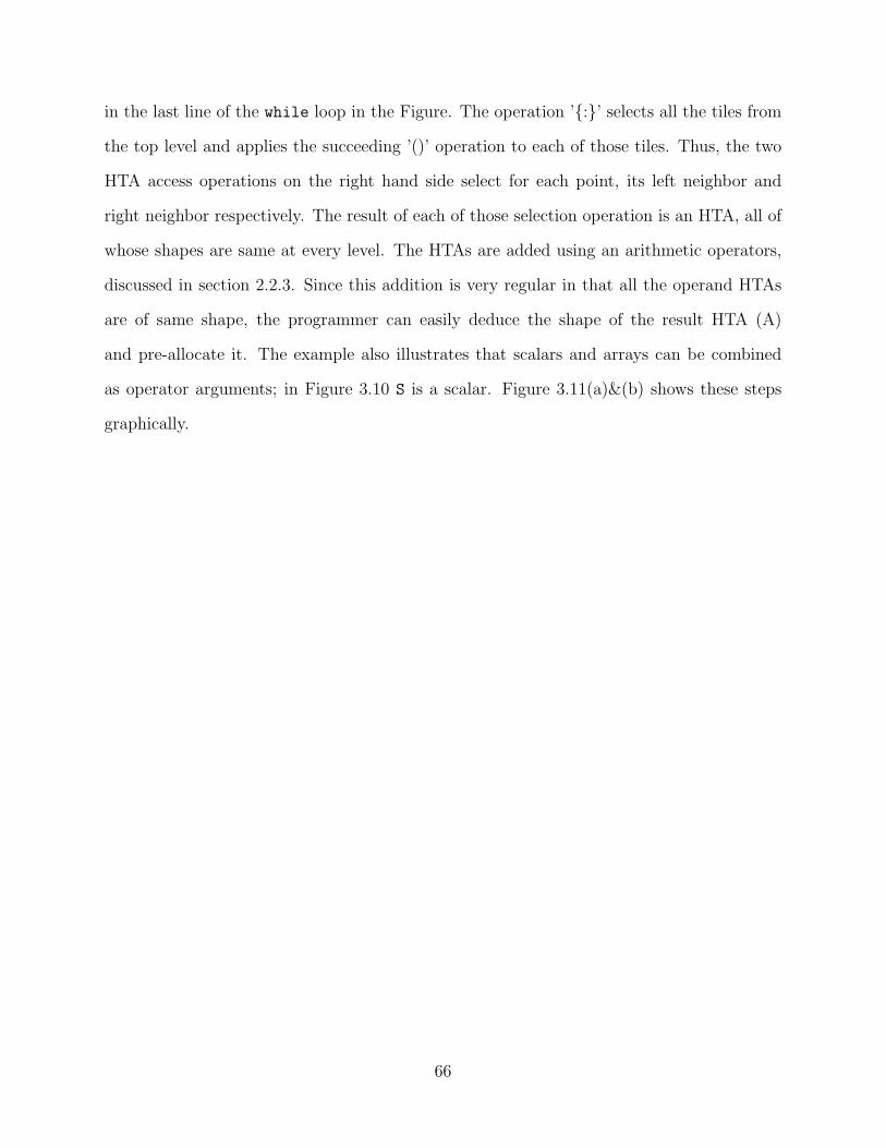
in the last line of the while loop in the Figure. The operation ’{:}’ selects all the tiles from
the top level and applies the succeeding ’()’ operation to each of those tiles. Thus, the two
HTA access operations on the right hand side select for each point, its left neighbor and
right neighbor respectively. The result of each of those selection operation is an HTA, all of
whose shapes are same at every level. The HTAs are added using an arithmetic operators,
discussed in section 2.2.3. Since this addition is very regular in that all the operand HTAs
are of same shape, the programmer can easily deduce the shape of the result HTA (A)
and pre-allocate it. The example also illustrates that scalars and arrays can be combined
as operator arguments; in Figure 3.10 S is a scalar. Figure 3.11(a)&(b) shows these steps
graphically.
66

Chapter 4
Evaluation
4.1 Introduction
In this chapter we demonstrate the expressive power of HTAs by using it to write several non-
trivial parallel programs. The programs are from the NAS benchmarks suite [7] developed
by NASA. These are a set of programs that were designed to evaluate the performance of
parallel supercomputers [7]. We have implemented the following seven of the eight programs
in the NAS benchmarks using HTAs: EP, MG, CG, FT, IS, BT, and LU. Table 4.1 lists the
characteristics of the computation and communication patterns in each of these programs.
Our implementation of the benchmark programs follows the same strategy as the public-
domain MPI implementation of the NAS benchmarks [7]. For each benchmark we developed
a serial version in MATLAB and extended it to use HTAs. Both MATLAB+HTA and C++-
HTA versions are obtained from the MATLAB serial versions. Several transformations were
applied in the serial code to obtain the tiled parallel versions of the programs. The list of
transformations are given below :
• Vetorization : The first step in the rewriting of the NAS benchmarks programs is to
replace all the loops in the scalar F77 programs with corresponding vector operations.
Table 4.1: Characteristics of Computation and Communication of the programs of NAS benchmark set.
Benchmark Description Computation Pattern Communication Pattern
EP Random number generation Random number generation ReductionMG Multi Grid V-cycle algorithm 3D Convolutions Nearest neighborCG Conjugate Gradient algorithm Sparse Matrix vector multiplication ReductionFT 3D Fourier transform Fourier transform Array TranspositionIS Linear time sorting of integer keys Bucket sort Reduction, scanBT Navier Stokes Equation Solver Tri diagonal Gaussian Elimination Nearest neighborLU Navier Stokes Equation Solver Symmetric Successive Over Relaxation Nearest neighbor
67
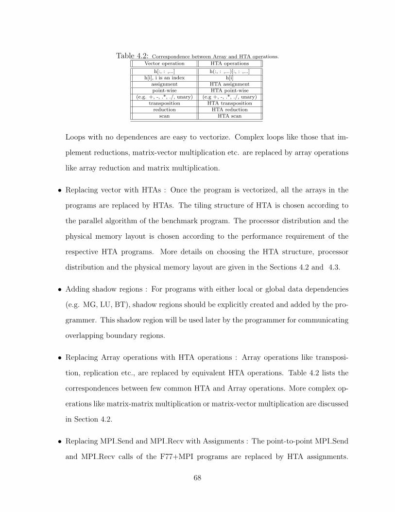
Table 4.2: Correspondence between Array and HTA operations.
Vector operation HTA operations
h[:, : ,...] h(:, : ,...)[:, : ,...]h[i], i is an index h[i]
assignment HTA assignmentpoint-wise HTA point-wise
(e.g. +, -, .*, ./, unary) (e.g +, -, .*, ./, unary)transposition HTA transposition
reduction HTA reductionscan HTA scan
Loops with no dependences are easy to vectorize. Complex loops like those that im-
plement reductions, matrix-vector multiplication etc. are replaced by array operations
like array reduction and matrix multiplication.
• Replacing vector with HTAs : Once the program is vectorized, all the arrays in the
programs are replaced by HTAs. The tiling structure of HTA is chosen according to
the parallel algorithm of the benchmark program. The processor distribution and the
physical memory layout is chosen according to the performance requirement of the
respective HTA programs. More details on choosing the HTA structure, processor
distribution and the physical memory layout are given in the Sections 4.2 and 4.3.
• Adding shadow regions : For programs with either local or global data dependencies
(e.g. MG, LU, BT), shadow regions should be explicitly created and added by the pro-
grammer. This shadow region will be used later by the programmer for communicating
overlapping boundary regions.
• Replacing Array operations with HTA operations : Array operations like transposi-
tion, replication etc., are replaced by equivalent HTA operations. Table 4.2 lists the
correspondences between few common HTA and Array operations. More complex op-
erations like matrix-matrix multiplication or matrix-vector multiplication are discussed
in Section 4.2.
• Replacing MPI Send and MPI Recv with Assignments : The point-to-point MPI Send
and MPI Recv calls of the F77+MPI programs are replaced by HTA assignments.
68

At present, the communication of the boundary regions for programs like MG (which
implements the stencil computation) is done by explicit assignment operation. As
a future work, overlapped tiling mechanism is under study [35]. This will free the
programmer from performing explicit assignments for boundary exchanges.
• Replacing MPI Reduce with HTA reduce : MPI reductions are replaced by HTA re-
duction. MPI reductions are not array reductions. They do not assume any topology
over which they perform the reduction. Based on the algorithm of the program, the
type and dimension of the reductions are deduced.
The remainder of the chapter is organized as follows. Section 4.2 discusses the main
characteristics of the HTA implementation for each benchmark. In Section 4.3 an empirical
comparison of HTA and MPI programs is presented. We use the execution time of the
parallel programs as the metric. In Section 4.4 we argue that tiling leads to programs with
better readability. For this, we compare the source lines of code in the FORTRAN+MPI
version with that of the MATLAB+HTA and CPP+HTA programs.
4.2 Description of the NAS benchmark programs
In this section, we present a description of the NAS programs written using HTAs. We
present the core algorithm behind each NAS benchmark program and show several code
snippets of the HTA programs. For simplicity and clarity, the codes from our MATLAB
implementation are shown; C++ version is shown in certain special cases either to emphasize
a concept or a new construct absent in the MATLAB version.
4.2.1 EP
EP is an embarrassingly parallel benchmark. It can be used to determine the peak parallel
performance of a machine. EP generates Gaussian random numbers using the Algorithm 9.
It generates N pairs of uniform pseudo random numbers in the interval (0, 1). These numbers
69

(1, −1)(−1,−1)(1, −1)(−1,−1)
(−1,1) (1,1)
P2
(−1,1) (1,1)
P1 P3
(−10, 10)
(−10, −10)
(10, 10)
(10, −10)
(a)
(b)
(0,0) (0,1)
(1,0) (1,1)
Figure 4.1: (a) Illustration of the EP algorithm. (b) Sequence splitting algorithm for gener-ation random numbers in parallel
are then scaled to the interval (−1, 1) using the transformation (2ai − 1, 2bi − 1). From the
resulting pairs (xj, yj), those that fall within the unit circle x2 + y2 = 1 are chosen and the
following transformation is applied.
Xj = xj
√(−2 log tj/tj) (4.1)
Yj = yj
√(−2 log tj/tj) (4.2)
where,
tj = x2j + y2
j
From the resulting pairs of (Xi, Yi) those that fall within successive square annuli are
tabulated.
l ≤ max (|X|, |Y |) < l + 1, 0 < l < 9 (4.3)
70
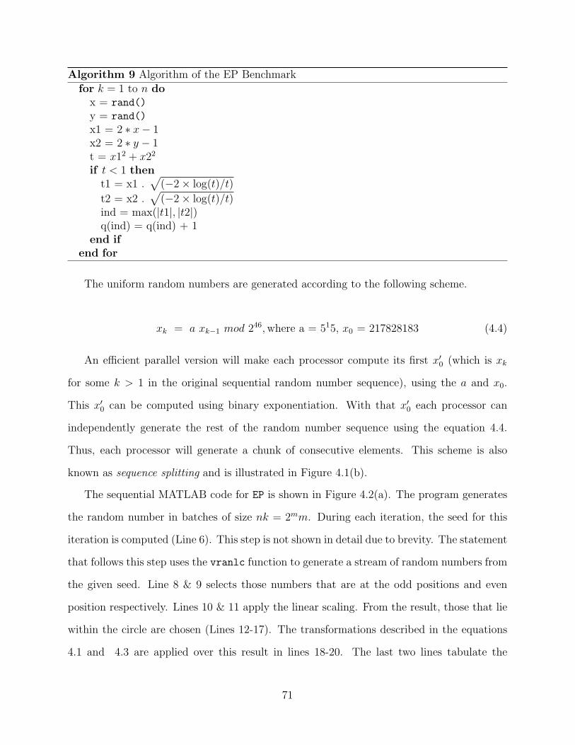
Algorithm 9 Algorithm of the EP Benchmark
for k = 1 to n dox = rand()
y = rand()
x1 = 2 ∗ x− 1x2 = 2 ∗ y − 1t = x12 + x22
if t < 1 thent1 = x1 .
√(−2× log(t)/t)
t2 = x2 .√
(−2× log(t)/t)ind = max(|t1|, |t2|)q(ind) = q(ind) + 1
end ifend for
The uniform random numbers are generated according to the following scheme.
xk = a xk−1 mod 246, where a = 515, x0 = 217828183 (4.4)
An efficient parallel version will make each processor compute its first x′0 (which is xk
for some k > 1 in the original sequential random number sequence), using the a and x0.
This x′0 can be computed using binary exponentiation. With that x′0 each processor can
independently generate the rest of the random number sequence using the equation 4.4.
Thus, each processor will generate a chunk of consecutive elements. This scheme is also
known as sequence splitting and is illustrated in Figure 4.1(b).
The sequential MATLAB code for EP is shown in Figure 4.2(a). The program generates
the random number in batches of size nk = 2mm. During each iteration, the seed for this
iteration is computed (Line 6). This step is not shown in detail due to brevity. The statement
that follows this step uses the vranlc function to generate a stream of random numbers from
the given seed. Line 8 & 9 selects those numbers that are at the odd positions and even
position respectively. Lines 10 & 11 apply the linear scaling. From the result, those that lie
within the circle are chosen (Lines 12-17). The transformations described in the equations
4.1 and 4.3 are applied over this result in lines 18-20. The last two lines tabulate the
71

1 function ep
2 ...
3 for k = 0:np-1
4 kk = k_offset + k;
5 %find the seed for this iteration
6 t1 = seed (kk, s, an);
7 [x, t1] = vranlc (2*nk, t1, a);
8 odd = x(1:2:end);
9 even = x(2:2:end);
10 x1 = 2 * odd - 1.d0;
11 x2 = 2 * even - 1.d0;
12 xt1 = x1 .^ 2;
13 xt2 = x2 .^ 2;
14 t = xt1 + xt2;
15 x1 = x1(t <= 1);
16 x2 = x2(t<= 1);
17 t2 = t(t <= 1);
18 t3 = sqrt( (-2.d0 .* (log(t2) ./ t2)) );
19 t4 = x1 .* t3;
20 t5 = x2 .* t3;
21 tt = fix(max(abs(t4), abs(t5)));
22 q = q + accumarray(tt+1,1,[nq 1]);
23 end
(a)
function ep
...
for k = 1:np
kk = k_offset + k;
%find the global seed for this iteration
t1 = map (@seed, kk, s, an );
[x, t1] = map ( @vranlc, 2*nk, t1, a);
odd = x{:,:}(1, 1:2:2^(mk+1));
even = x{:,:}(1, 2:2:2^(mk+1));
x1 = 2 .* odd - 1.d0;
x2 = 2 .* even - 1.d0;
xt1 = x1 .^ 2;
xt2 = x2 .^ 2;
t = xt1 + xt2;
x1 = x1{:,:}(t <= 1);
x2 = x2{:,:}(t<= 1 );
t2 = t{:,:}(t <= 1);
t3 = sqrt( (-2.d0 .* (log(t2) ./ t2)) );
t4 = x1 .* t3;
t5 = x2 .* t3;
tt = fix(max (abs(t4), abs(t5)));
q = q + accumarray(tt+1,1,[10 1]));
end
r = reduce(@sum, q, 2, false );
(b)
Figure 4.2: NAS EP benchmark using HTA (a) MATLAB-serial (b) MALAB-HTA
numbers that lie in successive square annuli according to the equation 4.3. accumarray
(IND, VAL, SZ) is a MATLAB function that creates an array of size SZ and fills the array
by accumulating the value VAL repeatedly at the subscripts specified by IND.
The HTA version of this code is shown in Figure 4.2(b). The version is different from the
serial version in the usage of HTA and HTA operations instead of array and array operations.
The vectors are converted into HTA of rank 1 with row-cyclic distribution. The vranlc is
replaced by a call to map, that in turn calls vranlc on each tile. Array selection operations
like x1(t<=1) are replaced by HTA selection operations like x1{:,:}(t < =1), where both
x1 and t are HTAs. Lastly, a reduce statement is used at the end to combine the results
over all the tiles, which is not required in sequential case.
A simpler and more efficient way to express these computations is to use map function for
the entire set of computation, as shown in Figure 4.3. Both the random number generation
and tabulation of the Gaussian deviates are written in a function that is applied to each tile
of an HTA using map. The result is an HTA, q that contains the local count of each tile.
The reduction of q using the reduce method call yields the global count.
72
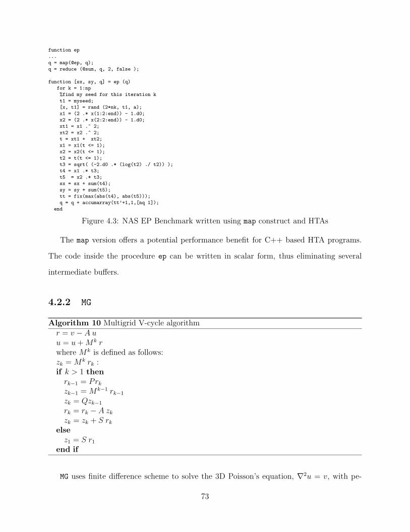
function ep
...
q = map(@ep, q);
q = reduce (@sum, q, 2, false );
function [sx, sy, q] = ep (q)
for k = 1:np
%find my seed for this iteration k
t1 = myseed;
[x, t1] = rand (2*nk, t1, a);
x1 = (2 .* x(1:2:end)) - 1.d0;
x2 = (2 .* x(2:2:end)) - 1.d0;
xt1 = x1 .^ 2;
xt2 = x2 .^ 2;
t = xt1 + xt2;
x1 = x1(t <= 1);
x2 = x2(t <= 1);
t2 = t(t <= 1);
t3 = sqrt( (-2.d0 .* (log(t2) ./ t2)) );
t4 = x1 .* t3;
t5 = x2 .* t3;
sx = sx + sum(t4);
sy = sy + sum(t5);
tt = fix(max(abs(t4), abs(t5)));
q = q + accumarray(tt’+1,1,[nq 1]);
end
Figure 4.3: NAS EP Benchmark written using map construct and HTAs
The map version offers a potential performance benefit for C++ based HTA programs.
The code inside the procedure ep can be written in scalar form, thus eliminating several
intermediate buffers.
4.2.2 MG
Algorithm 10 Multigrid V-cycle algorithmr = v − A uu = u + Mk rwhere Mk is defined as follows:zk = Mk rk :if k > 1 then
rk−1 = Prk
zk−1 = Mk−1 rk−1
zk = Qzk−1
rk = rk − A zk
zk = zk + S rk
elsez1 = S r1
end if
MG uses finite difference scheme to solve the 3D Poisson’s equation, ∇2u = v, with pe-
73
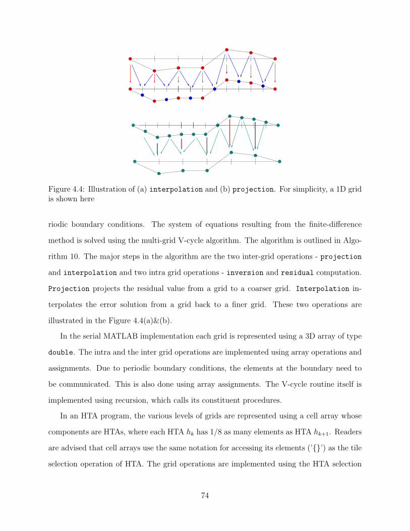
Figure 4.4: Illustration of (a) interpolation and (b) projection. For simplicity, a 1D gridis shown here
riodic boundary conditions. The system of equations resulting from the finite-difference
method is solved using the multi-grid V-cycle algorithm. The algorithm is outlined in Algo-
rithm 10. The major steps in the algorithm are the two inter-grid operations - projection
and interpolation and two intra grid operations - inversion and residual computation.
Projection projects the residual value from a grid to a coarser grid. Interpolation in-
terpolates the error solution from a grid back to a finer grid. These two operations are
illustrated in the Figure 4.4(a)&(b).
In the serial MATLAB implementation each grid is represented using a 3D array of type
double. The intra and the inter grid operations are implemented using array operations and
assignments. Due to periodic boundary conditions, the elements at the boundary need to
be communicated. This is also done using array assignments. The V-cycle routine itself is
implemented using recursion, which calls its constituent procedures.
In an HTA program, the various levels of grids are represented using a cell array whose
components are HTAs, where each HTA hk has 1/8 as many elements as HTA hk+1. Readers
are advised that cell arrays use the same notation for accessing its elements (’{}’) as the tile
selection operation of HTA. The grid operations are implemented using the HTA selection
74

r5 r4 r3 r2 r1
d=[1,1]
d=[1,1]
d=[2,2]
d=[2,1]
Figure 4.5: Pictorial view of HTA projection
function [uout] = mg3p(r, u, k)
if( k > 1 )
r{k-1} = rprj3(r{k}, r{k-1});
u{k-1} = mg3p(r, u, k-1);
u{k} = interp(u{k-1}, u{k});
r{k} = resid(u{k}, r{k});
u{k} = psinv(r{k}, u{k});
else
u{1} = psinv(r{1}, u{1});
end
Figure 4.6: The main procedure of MG in MATLAB
and addition operations. A pictorial view of the projection function in an HTA program
is shown in Figure 4.5-(a)&(b) for a 2D grid. Each highlighted grid point in HTA r4 in
Figure 4.5-(a) is computed as the weighted average of the grid point itself and all its neighbors
in HTA r5, as shown in the zoomed HTA, where the shadow regions to allocate the data
from the neighbors HTA are also shown.
Figures 4.7- 4.10 show the code for inversion, residual computation, projection and
interpolation operations. In the figures, the corresponding functions are psinv, resid,
rprj3 and interp respectively. Each of the figure lists the code for the MATLAB-serial and
the MATLAB+HTA versions. For clarity, some details are removed from the codes.
Figure 4.6 shows the top level V-cycle routine in MATLAB. For each grid at level k, the
rprj3 function is called until it reaches the grid at level 0. At this point the recursion ends
75

function r = resid( u, v)
I = 2:n1-1;
J = 2:n2-1;
K = 2:n3-1;
u1 = u(1:n1,J-1,K) + u(1:n1,J+1, K)
+ u(1:n1, J, K-1) + u(1:n1, J, K+1);
u2 = u(1:n1,J-1, K-1) + u(1:n1, J+1, K-1)
+ u(1:n1, J-1, K+1) + u(1:n1,J+1, K+1);
u(I, J, K) = a(1) * u(I, J, K)
+ a(3) * (u2(I, :, :)
+ u1(I-1, :, :)
+ u1(I+1,:,:))
+ a(4) * (u2(I-1,:,:)
+ u2(I+1,:,:));
r = v - u;
r = comm3(r);(a)
function r = resid( u, v)
I = 2:n1-1;
J = 2:n2-1;
K = 2:n3-1;
u1 = u{:,:,:}(1:n1,J-1,K) + u{:,:,:}(1:n1,J+1, K)
+ u{:,:,:}(1:n1, J, K-1) + u{:,:,:}(1:n1, J, K+1);
u2 = u{:,:,:}(1:n1,J-1, K-1) + u{:,:,:}(1:n1, J+1, K-1)
+ u{:,:,:}(1:n1, J-1, K+1) + u{:,:,:}(1:n1,J+1, K+1);
u{:,:,:}(I, J, K) = a(1) * u{:,:,:}(I, J, K)
+ a(3) * (u2{:,:,:}(I, :, :)
+ u1{:,:,:}( I-1, :, :)
+ u1{:,:,:}(I+1,:,:))
+ a(4) * (u2{:,:,:}(I-1,:,:)
+ u2{:,:,:}(I+1,:,:) );
r = v - u;
r = comm3(r);(b)
Figure 4.7: MG resid (a) MATLAB-serial version (b) MATLAB+HTA version
function u = psinv( r, u)
I = 2:n1-1;
J = 2:n2-1;
K = 2:n3-1;
r1 = r(1:n1,J-1,K) + r(1:n1,J+1, K)
+ r(1:n1, J, K-1) + r(1:n1, J, K+1);
r2 = r(1:n1,J-1, K-1) + r(1:n1, J+1, K-1)
+ r(1:n1, J-1, K+1) + r(1:n1,J+1, K+1);
r(I, J, K) = c(1) * r(I, J, K)
+ c(2) * (r(I-1, J, K)
+ r( I+1, J, K)
+ r1(I,:,:))
+ c(3) * (r2(I,:,:)
+ r1(I-1,:,:)
+ r1(I+1,:,:));
u = u + r;
u=comm3(u);(a)
function u = psinv( r, u)
I = 2:n1-1;
J = 2:n2-1;
K = 2:n3-1;
r1 = r{:,:,:}(1:n1,J-1,K) + r{:,:,:}(1:n1,J+1, K)
+ r{:,:,:}(1:n1, J, K-1) + r{:,:,:}(1:n1, J, K+1);
r2 = r{:,:,:}(1:n1,J-1, K-1) + r{:,:,:}(1:n1, J+1, K-1)
+ r{:,:,:}(1:n1, J-1, K+1) + r{:,:,:}(1:n1,J+1, K+1);
r{:,:,:}(I, J, K) = c(1) * r{:,:,:}(I, J, K)
+ c(2) * (r{:,:,:}(I-1, J, K)
+ r{:,:,:}( I+1, J, K)
+ r1{:,:,:}(I,:,:) )
+ c(3) * (r2{:,:,:}(I,:,:)
+ r1{:,:,:}(I-1,:,:)
+ r1{:,:,:}(I+1,:,:) );
u = u + r;
u = comm3(u);(b)
Figure 4.8: MG psinv (a) MATLAB-serial version (b) MATLAB+HTA version
and the interpolation, resid and psinv functions are called on increasingly finer grids.
Both the serial and the HTA versions use the same variable names for the index bounds
(n1, n2, and n3). However, their values for the HTA version is smaller than that of the serial
version, as they operate on a restricted domain distributed on each processor. Additionally,
both the number of processor and the problem size are powers of two and hence the problem
size is perfectly divisible by the number of processors. The boundary conditions are also
periodic. As a result, the size of all the tiles is the same (i.e., the HTA is homogeneous
and regular). This lead to the usage of HTA element access operation and the data parallel
arithmetic operations easily for the stencil computation.
76

function s = rprj3 (r, s)
RI = 2*2-1:2:2*m1j-1;
RJ = 2*2-1:2:2*(m2j-1)-1;
RK = 2*2-1:2:2*(m3j-1)-1;
x1 = r(RI-1,RJ-1,RK)
+ r(RI-1,RJ+1,RK)
+ r(RI-1, RJ, RK-1)
+ r(RI-1, RJ, RK+1);
y1 = r(RI-1,RJ-1,RK-1)
+ r(RI-1,RJ-1, RK+1)
+ r(RI-1,RJ+1,RK-1)
+ r(RI-1,RJ+1,RK+1);
RI = 2*2-d1:2:2*(m1j-1)-d1;
y2 = r(RI, RJ-1, RK-1)
+ r(RI, RJ-1, RK+1)
+ r(RI, RJ+1, RK-1)
+ r(RI, RJ+1, RK+1);
x2 = r(RI, RJ-1, RK)
+ r(RI, RJ+1, RK)
+ r(RI, RJ, RK-1)
+ r(RI, RJ, RK+1);
s(SI, SJ, SK) = 0.5D0 * r(RI,RJ,RK)
+ 0.25D0 * (r(RI-1,RJ, RK)
+ r(RI+1, RJ, RK) + x2)
+ 0.125D0 * (x1(SI-1, :, :)
+ x1(SI,:, :) + y2)
+ 0.0625D0 * (y1(SI-1, :, :)
+ y1(SI, :, :)
s = comm3(s);(a)
function s = rprj3( r, s )
RI = 2*2-1:2:2*m1j-1;
RJ = 2*2-1:2:2*(m2j-1)-1;
RK = 2*2-1:2:2*(m3j-1)-1;
x1 = r{:,:,:}(RI-1,RJ-1,RK)
+ r{:,:,:}(RI-1,RJ+1,RK)
+ r{:,:,:}(RI-1, RJ, RK-1)
+ r{:,:,:}(RI-1, RJ, RK+1);
y1 = r{:,:,:}(RI-1,RJ-1,RK-1)
+ r{:,:,:}(RI-1,RJ-1, RK+1)
+ r{:,:,:}(RI-1,RJ+1,RK-1)
+ r{:,:,:}(RI-1,RJ+1,RK+1);
RI = 2*2-1:2:2*(m1j-1)-1;
y2 = r{:,:,:}(RI, RJ-1, RK-1)
+ r{:,:,:}(RI, RJ-1, RK+1)
+ r{:,:,:}(RI, RJ+1, RK-1)
+ r{:,:,:}(RI, RJ+1, RK+1);
x2 = r{:,:,:}(RI, RJ-1, RK)
+ r{:,:,:}(RI, RJ+1, RK)
+ r{:,:,:}(RI, RJ, RK-1)
+ r{:,:,:}(RI, RJ, RK+1);
SI = 2:m1j-1;
SJ = 2:m2j-1;
SK = 2:m3j-1;
s{:,:,:}(SI, SJ, SK) = 0.5D0 * r{:,:,:}(RI,RJ,RK)
+ 0.25D0 * ( r{:,:,:}(RI-1,RJ, RK)
+ r{:,:,:}(RI+1, RJ, RK) + x2)
+ 0.125D0 * ( x1{:,:,:}(SI-1, :, :)
+ x1{:,:,:}(SI,:, :) + y2)
+ 0.0625D0 * ( y1{:,:,:}(SI-1, :, :)
+ y1{:,:,:}(SI, :, :) );
s = comm3( s );(b)
Figure 4.9: MG rprj3 (a) MATLAB-serial version (b) MATLAB+HTA version
The communication of the boundary region is performed using HTA assignments as
shown in the Figure 4.11. comm3 performs the assignment of the boundary regions in a given
direction. For example, in Figure 4.12(a)&(b) the assignments are performed along the west
and north directions.
The MPI version of MG requires the programmer to allocate the boundary regions himself
and use MPI Send and MPI Recv to communicate the boundary regions. Moreover, since
MG uses periodic boundary conditions, the communication for boundary processors has to be
handled differently.
Further more, as the coarsening proceeds there will be a point when the number of
77

function u = interp( z, u )
UI = 1:2:2*(mm1-1)-1;
UJ = 1:2:2*(mm2-1)-1;
UK = 1:2:2*(mm3-1)-1;
ZI = 1:mm1-1;
ZJ = 1:mm2-1;
ZK = 1:mm3-1;
z1 = z(1:mm1,2:mm2,1:mm3-1)
+ z(1:mm1,1:mm2-1,1:mm3-1);
z2 = z(1:mm1,1:mm2-1,2:mm3)
+ z(1:mm1,1:mm2-1,1:mm3-1);
z3 = z(1:mm1,2:mm2,2:mm3)
+ z(1:mm1,1:mm2-1,2:mm3)
+ z1(1:mm1,1:mm2-1,1:mm3-1);
u(UI, UJ, UK) = z(ZI, ZJ, ZK);
u(UI+1, UJ, UK) = 0.5*(z(ZI+1,ZJ,ZK)
+z(ZI,ZJ,ZK));
u(UI, UJ+1,UK) = 0.5 * z1(ZI,ZJ,ZK);
u(UI+1, UJ+1,UK) = 0.25*( z1(ZI, ZJ, ZK)
+ z1(ZI+1,ZJ, ZK) );
u(UI, UJ, UK+1) = 0.5 * z2(ZI, ZJ, ZK);
u(UI+1, UJ, UK+1) = 0.25*( z2(ZI, ZJ, ZK)
+ z2(ZI+1, ZJ, ZK) );
u(UI, UJ+1,UK+1) = 0.25* z3(ZI, ZJ, ZK);
u(UI+1, UJ+1, UK+1) = 0.125*( z3(ZI, ZJ, ZK)
+ z3(ZI+1, ZJ, ZK));(a)
function u = interp (z, u)
UI = 1:2:2*(mm1-1)-1;
UJ = 1:2:2*(mm2-1)-1;
UK = 1:2:2*(mm3-1)-1;
ZI = 1:mm1-1;
ZJ = 1:mm2-1;
ZK = 1:mm3-1;
z1 = z{:,:,:}(1:mm1,ZJ+1,ZK)
+ z{:,:,:}(1:mm1,ZJ,ZK);
z2 = z{:,:,:}(1:mm1,ZJ,ZK+1)
+ z{:,:,:}(1:mm1,ZJ,ZK);
z3 = z{:,:,:}(1:mm1,ZJ+1,ZK+1)
+ z{:,:,:}(1:mm1, ZJ,ZK+1)
+ z1{:,:,:}(1:mm1,ZJ,ZK);
u{:,:,:}(UI, UJ, UK) = z{:,:,:}(ZI, ZJ, ZK);
u{:,:,:}(UI+1, UJ, UK) = 0.5 * (z{:,:,:}(ZI+1,ZJ,ZK)
+ z{:,:,:}(ZI,ZJ,ZK));
u{:,:,:}(UI, UJ+1,UK) = 0.5 * z1{:,:,:}(ZI,ZJ,ZK);
u{:,:,:}(UI+1, UJ+1,UK) = 0.25 * (z1{:,:,:}(ZI, ZJ, ZK)
+ z1{:,:,:}(ZI+1,ZJ, ZK));
u{:,:,:}(UI, UJ, UK+1) = 0.5 * z2{:,:,:}(ZI, ZJ, ZK);
u{:,:,:}(UI+1, UJ, UK+1) = 0.25 * (z2{:,:,:}(ZI, ZJ, ZK)
+ z2{:,:,:}(ZI+1, ZJ, ZK));
u{:,:,:}(UI, UJ+1,UK+1) = 0.25 * z3{:,:,:}(ZI, ZJ, ZK);
u{:,:,:}(UI+1, UJ+1, UK+1) = 0.125 * (z3{:,:,:}(ZI, ZJ, ZK)
+ z3{:,:,:}(ZI+1, ZJ, ZK));(b)
Figure 4.10: MG interp (a) MATLAB-serial version (b) MATLAB+HTA version
grid points become lesser than the number of processors. In those cases, only a subset of
the processors participate in the computation. Also, the processors do not exchange data
with immediate neighbors, but with the second or forth and so on. All these require the
programmer to insert extra logic. With HTAs this is very easy to express this. For this corner
case, we can create HTAs of different topology than those created for normal case. Inter-grid
operation between such HTAs and the normal HTAs can be implemented by using element
access operations, which will select only the tiles that need to participate in a computation
step.
The processor distribution for the normal HTAs is row-cyclic. For the corner case
HTAs, the processor distribution is chosen so that when operating with the normal HTAs,
the operation involves no or minimal communication. For example, referring to Figure 4.5,
the tiles 0 and 1 of the HTA r1 reside in the home nodes of the tiles 1 and 3 of the HTA
r2. This is because, during rprj3 and interp, these are the tiles that participate in the
computation. All the HTAs are created apriori and the required processor distribution is
78
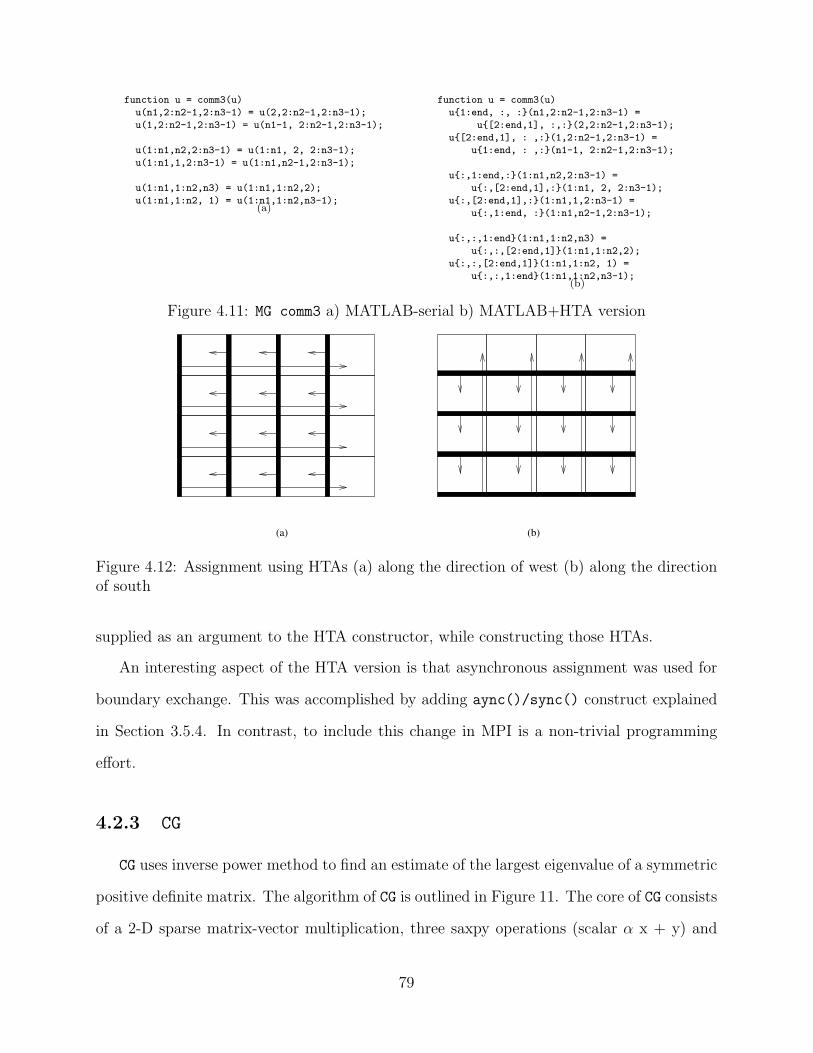
function u = comm3(u)
u(n1,2:n2-1,2:n3-1) = u(2,2:n2-1,2:n3-1);
u(1,2:n2-1,2:n3-1) = u(n1-1, 2:n2-1,2:n3-1);
u(1:n1,n2,2:n3-1) = u(1:n1, 2, 2:n3-1);
u(1:n1,1,2:n3-1) = u(1:n1,n2-1,2:n3-1);
u(1:n1,1:n2,n3) = u(1:n1,1:n2,2);
u(1:n1,1:n2, 1) = u(1:n1,1:n2,n3-1);(a)
function u = comm3(u)
u{1:end, :, :}(n1,2:n2-1,2:n3-1) =
u{[2:end,1], :,:}(2,2:n2-1,2:n3-1);
u{[2:end,1], : ,:}(1,2:n2-1,2:n3-1) =
u{1:end, : ,:}(n1-1, 2:n2-1,2:n3-1);
u{:,1:end,:}(1:n1,n2,2:n3-1) =
u{:,[2:end,1],:}(1:n1, 2, 2:n3-1);
u{:,[2:end,1],:}(1:n1,1,2:n3-1) =
u{:,1:end, :}(1:n1,n2-1,2:n3-1);
u{:,:,1:end}(1:n1,1:n2,n3) =
u{:,:,[2:end,1]}(1:n1,1:n2,2);
u{:,:,[2:end,1]}(1:n1,1:n2, 1) =
u{:,:,1:end}(1:n1,1:n2,n3-1);(b)
Figure 4.11: MG comm3 a) MATLAB-serial b) MATLAB+HTA version
(a) (b)
Figure 4.12: Assignment using HTAs (a) along the direction of west (b) along the directionof south
supplied as an argument to the HTA constructor, while constructing those HTAs.
An interesting aspect of the HTA version is that asynchronous assignment was used for
boundary exchange. This was accomplished by adding aync()/sync() construct explained
in Section 3.5.4. In contrast, to include this change in MPI is a non-trivial programming
effort.
4.2.3 CG
CG uses inverse power method to find an estimate of the largest eigenvalue of a symmetric
positive definite matrix. The algorithm of CG is outlined in Figure 11. The core of CG consists
of a 2-D sparse matrix-vector multiplication, three saxpy operations (scalar α x + y) and
79
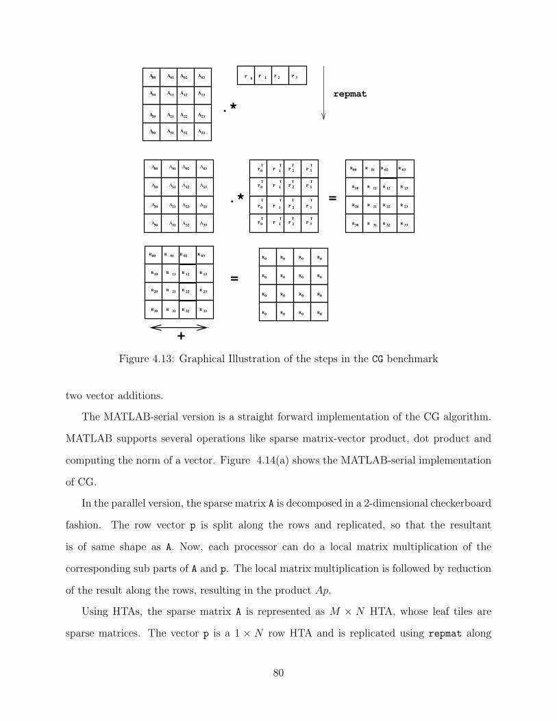
A
A
A
A A
A A
A
A
A
A A
00
10 A 11 12 13
23
33 32 31 A
21 22
30
A 20
A 01 02 03
R 0 R 0 R 0 0 R
R 0 R 0 R 0 0 R
R 0 R 0 R 0 0 R
R 0 R 0 R 0 0 R
TT T T
TT T T
TT T T
TT T T P 1 2 P 3 P P 0
0
0
0 P 1 2 P 3 P
P 1 2 P 3 P
P 1 2 P 3 P
P
P
P
R 00 R 01 02 R 03 R
R 10 R 11 12 R 13 R
R 30 R 31 32 R 33 R
R 20 R 21 22 R 23 R
1 2 P 3 P P 0 P
R 00 R 01 02 R 03 R
R 10 R 11 12 R 13 R
R 30 R 31 32 R 33 R
R 20 R 21 22 R 23 R
=
repmat
.*
.*
=
+
A A A A
A A A A
A A A
A A A A
03
13
23
33 32
22
12
02 01
11
21
31
A
10
00
20
30
Figure 4.13: Graphical Illustration of the steps in the CG benchmark
two vector additions.
The MATLAB-serial version is a straight forward implementation of the CG algorithm.
MATLAB supports several operations like sparse matrix-vector product, dot product and
computing the norm of a vector. Figure 4.14(a) shows the MATLAB-serial implementation
of CG.
In the parallel version, the sparse matrix A is decomposed in a 2-dimensional checkerboard
fashion. The row vector p is split along the rows and replicated, so that the resultant
is of same shape as A. Now, each processor can do a local matrix multiplication of the
corresponding sub parts of A and p. The local matrix multiplication is followed by reduction
of the result along the rows, resulting in the product Ap.
Using HTAs, the sparse matrix A is represented as M × N HTA, whose leaf tiles are
sparse matrices. The vector p is a 1 × N row HTA and is replicated using repmat along
80

Algorithm 11 Conjugate Gradient Methodr = xρ = rT rp = rfor i = 1 to 25 do
q = Apα = ρ/(pT q)z = z + αpρ0 = ρr = r − αqρ = rT rβ = ρ/ρ0
ρ = r + βpend forcompute residual norm explicitly: ||r|| = ||x− Az||.
the columns, resulting in M × N HTA. Each of tiles of the resulting HTA p is transposed,
using the transpose coupled with map. Then, the operation map (*) (tile-by-tile matrix
multiplication) is applied to A and p. This is followed by reduction along the rows using the
reduce method call. The entire process is shown in the Figure 4.13. A following statement
requires the computation of pT q. In the case of HTA program, this is achieved by transposing
the result q, applying the tile-by-tile matrix multiplication operation, followed by reduction
across rows. It may be recalled that the vector p is already stored as a row vector. The
other operations like computing the norm and saxpy are implemented similarly using the
HTA operations defined earlier in Chapter 2.
The implementation of this benchmark is greatly simplified by Sparse HTAs. Sparse
HTAs are HTAs whose tiles are sparse matrices. They are constructed in a similar fashion as
dense HTAs, with only the type of the HTA being different. All the normal HTA operations
are defined for sparse HTAs also and are implemented by the library differently. Thus, the
programmer is decoupled from all the low level details of a sparse matrix and is required
to provide only the high level algorithm. The complete code for the HTA version of the
conjugate gradient routine is listed in Figure 4.14(b).
In contrast, the MPI version of CG listed in Figure 1 (Appendix) is too low level and
81

function rnorm = conj_grad(x, c)
z = 0;
r = x;
p = r;
rho = r*r’;
for cgit = 1:cgitmax
rho0=rho;
d=0;
q=(c*p’)’;
d=d+p*q’;
alpha = rho0 ./ d;
z = z + alpha .* p;
r = r - alpha .* q;
rho = r*r’;
beta = rho./rho0;
p = r + beta*p;
end
r=(c*z’)’;
f = x-r;
sumx=f*f’;
rnorm = sqrt(sumx); (a)
function rnorm = conj_grad(x, c)
z = 0;
r = x;
p = r;
rho = reduce(’sum’, r .^ 2, 2, true );
for cgit = 1:cgitmax
rho0 = rho;
qh = map (*, c, dottranspose(p));
qh = reduce( ’sum’, qh, 2, true );
qh = transpose (qh,[2 1]);
d = map (*, p dottranspose(qh));
d = reduce( ’sum’, d, 2, true );
alpha = rho0 ./ d;
z = z + alpha .* p;
r = r - alpha .* qh{:,:}(1,:);
rho = reduce( ’sum’, r .^ 2, 2, true );
beta = rho./rho0;
p = r + beta .* p;
end
r = map (*, c, dottranspose(z));
r = reduce( ’sum’,r,2,true);
r = transpose (r,[2 1]);
f = x - r;
sumx = reduce( ’sum’, f .^ 2, 2, true );
rnorm = sqrt(sumx); (b)
Figure 4.14: CG Benchmark (a) MATLAB-serial implementation (b) MATLAB+HTA im-plementation
difficult to comprehend. For simplicity, declaration of variables and parameters are ignored.
Due to the local view nature of MPI and the presence of message passing library calls,
the underlying algorithm is completely obscured by the code. Also, to gain performance
optimized library calls like non-blocking send and recv (e.g.MPI Isend) are used. This need
extra synchronization step, the negligence of which will lead to race condition, a very common
dreaded bug in parallel programs.
Moreover, the MPI version has extra code to handle the non-square partition of the
matrix A. When the number of processors (n) is an odd power of two, the MPI version maps
the domain in to a processor grid of size m× 2m. The pT q step requires redistribution of a
column spread across m processors in to a row spread across 2m processors. This requires
extra logic to be programmed. For an HTA program, the HTA can be represented always
as a square HTA and map 2 tiles per processor.
Given that a program like CG will be written only by scientists, the low level details
unrelated to his algorithm will discourage him from writing a parallel program. On the
82

function ft
...
xnt= fft (xnt, nx, 1 );
xnt= fft (xnt, ny, 2 );
xnt= fft (xnt, nz, 3 );
for kt = 1:niter
y = y .* twiddle;
xnt = y;
xnt= ifft (xnt, nx, 1 );
xnt= ifft (xnt, ny, 2 );
xnt= ifft (xnt, nz, 3 );
sums(kt) = checkSum (xnt, kt, nx,ny,nz);
end (a)
function ft
...
xnt = fft (xnt, [], 1 );
xnt = fft (xnt, [], 2 );
xnt = dtranspose (xnt,[ 3 1 2] );
xnt = fft (xnt, [], 1 );
for kt = 1:niter
y = y .* twiddle;
xnt = y;
xnt = ifft (xnt, [], 1 );
xnt = dtranspose (xnt,[2 3 1]);
xnt = ifft (xnt, [], 1 );
xnt = ifft (xnt [], 2 );
lsum = map (@checkSum, xnt);
sums(kt) = reduce (@sum, lsum, 0, false );
end
...(b)
Figure 4.15: FT Benchmark (a) HTA-serial version (b) MATLAB+HTA version
contrary, the HTA version correlates very well with the algorithmic description of the prob-
lem.Thus, HTAs not only save the programmer efforts, but also enables a programmer to
write complex parallel program. Apart from the programming convenience, it also provides
a means to write programs with optimal performance. For example, operations like pT q or
Ap can be implemented using matrix multiplication defined over HTAs. But this will lead
to unnecessary communication of the vectors among the processors during each step of the
iteration. Instead, the programmer can replicate the vectors in the beginning of the program
and perform a local tile-by-tile matrix multiplication, followed by reduction. Despite this
optimization, the programs look very clean and readable.
4.2.4 FT
The discrete Fourier transform is an important class of computation, widely used in image
processing and scientific applications. Fourier transform is the main computation in the FT
benchmark. FT solves partial differential equations (PDE) using forward and inverse Fourier
transform (FT). For more details on the problem, the readers are referred to [7]. Discrete
Fourier Transform (DFT) of a vector x of size n (also known as n-point DFT) is given by:
83

yi =n−1∑k=0
xkωki, 0 ≤ i < n (4.5)
In the above equation, ω is the primitive n-th root of unity; that is, ω = e2π√−1n.
Fourier transform of an m-dimensional array is computed as the Fourier transform of each
of its vectors in all the dimensions. The FT benchmark performs the following sequence of
computations. First, the Fourier transform of a 3D matrix is computed. This is followed
by multiplication of the result by a set of exponentials and computing the inverse Fourier
transform. The last step is repeated for several iterations. The inverse Fourier transform is
very similar to forward Fourier transform. The core computation of the serial version of the
FT benchmark is shown in the Figure 4.15(a). In the figure, fft is the standard MATLAB
procedure that computes the Fourier transform of all the vectors of the input matrix in the
given dimension.
All the steps in the FT benchmark, the computation of the forward and the inverse Fourier
transforms and the multiplication with the exponentials, can be parallelized. The parallel
Fourier transform of an m-dimensional array of size (N1 × N2 · · · ×Nm), decomposes the
array into tiles of size (N1 × N2
d2· · · ×Nm
dm), where di ≥ 1. FT along the first dimension
(unpartitioned) is just a local FT operation. To compute the FT along dimension i where
di > 1, the i − th dimension is transposed with the first dimension and the local FT is
applied along the first dimension. This algorithm is known as the Transpose algorithm.
The multiplication with the exponentials can be trivially parallelized by multiplying only
those sections of the array owned by a given processor.
In the HTA version, the array is decomposed in to an 3D-HTA, whose first dimension is
of size one. Figure 4.15(b) shows an outline of our implementation of this algorithm for a 3-D
array where only the third dimension of the HTA u is distributed, as shown in Figure 4.15(b).
FT along the first and second dimension of an HTA is computed using the overloaded version
of the standard MATLAB fft operator which applies the standard MATLAB fft to each of
the tiles of the HTA along the dimension specified in the third parameter. The overloaded
84
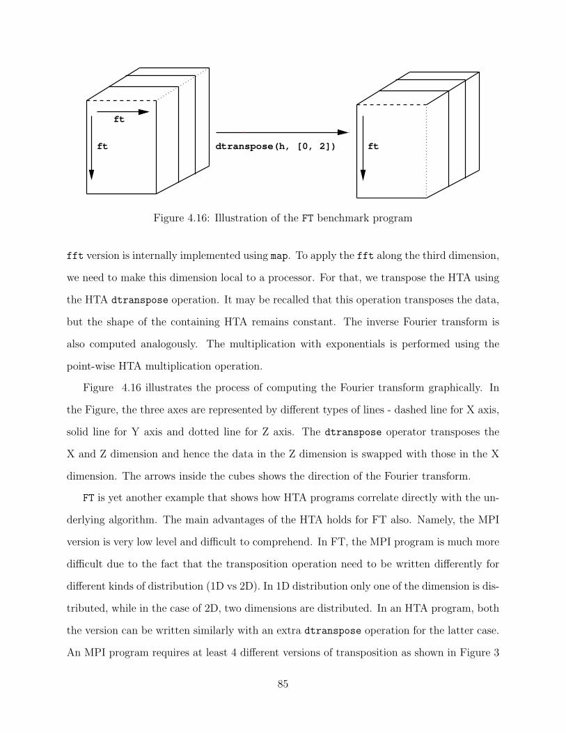
dtranspose(h, [0, 2])ft
ft
ft
Figure 4.16: Illustration of the FT benchmark program
fft version is internally implemented using map. To apply the fft along the third dimension,
we need to make this dimension local to a processor. For that, we transpose the HTA using
the HTA dtranspose operation. It may be recalled that this operation transposes the data,
but the shape of the containing HTA remains constant. The inverse Fourier transform is
also computed analogously. The multiplication with exponentials is performed using the
point-wise HTA multiplication operation.
Figure 4.16 illustrates the process of computing the Fourier transform graphically. In
the Figure, the three axes are represented by different types of lines - dashed line for X axis,
solid line for Y axis and dotted line for Z axis. The dtranspose operator transposes the
X and Z dimension and hence the data in the Z dimension is swapped with those in the X
dimension. The arrows inside the cubes shows the direction of the Fourier transform.
FT is yet another example that shows how HTA programs correlate directly with the un-
derlying algorithm. The main advantages of the HTA holds for FT also. Namely, the MPI
version is very low level and difficult to comprehend. In FT, the MPI program is much more
difficult due to the fact that the transposition operation need to be written differently for
different kinds of distribution (1D vs 2D). In 1D distribution only one of the dimension is dis-
tributed, while in the case of 2D, two dimensions are distributed. In an HTA program, both
the version can be written similarly with an extra dtranspose operation for the latter case.
An MPI program requires at least 4 different versions of transposition as shown in Figure 3
85
(Appendix): transpose xy z, transpose y xz, transpose x y and transpose x z. Also,
the transposition should be implemented using an optimized MPI method like MPI Alltoall;
point-to-point sends will lead to an sub-optimal O(P) communication complexity, where P
is the number of processors. In an HTA program, this decision is left to the run time library.
4.2.5 IS
Sorting is yet another class of computation that is widely used in practice. Given a sequence
of n numbers {a0, a1, a2, ...an−1}, the sorting problem is to find a permutation {a′0, a′1, a′2, ...a′n−1}
such that {a′0 ≤ a′1 ≤ a′2... ≤ a′n−1}. Many algorithms incorporate a sort so that information
may be accessed efficiently later.
IS benchmark performs ranking of random integers in a given range using bucket sort
algorithm. The integers are divided in to buckets, and are distributed across the processors.
They are partially sorted in each processor locally based on the first r most significant bits.
They are then divided in to sub-buckets of almost equal sizes. The sub-buckets are exchanged
among the processors, such that all the values in processor Pi is less than that of Pi+1. A
final sorting is done in each processor locally to result in the complete sorting of the original
data.
The above algorithm can be implemented in an HTA program using a two level HTA.
The top level is used as a means to describe the processor space, while the next level is
used for representing the bucket space. For IS we show the C-serial version and CPP-HTA
version instead of FORTRAN and MATLAB versions (Figure 4.17(a)&(b)).
The keys are in the range [0, Bmax), and are generated as follows. Let rf be a uniformly
distributed random number in the interval [0,1] and let Ki be the ith key. The value of Ki
is determined as
ki = bBmax(r4i+0 + r4i+1 + r4i+2 + r4i+3)/4c (4.6)
86

void rank() {
....
for( i=0; i<NUM_BUCKETS; i++ )
bucket_size[i] = 0;
for( i=0; i<NUM_KEYS; i++ )
{
int bucket = key_array[i]>>shift;
bucket_size[bucket]++;
}
bucket_ptrs[0] = 0;
for( i=1; i< NUM_BUCKETS; i++ )
bucket_ptrs[i] = bucket_ptrs[i-1] +
bucket_size[i-1];
partialsort (key_array, key_buff2);
key_buff_ptr2 = key_buff2;
....
localSort (key_buff_ptr2);
}
void bucketSort (key_array, key_buff2) {
for( i=0; i<NUM_KEYS; i++ )
{
int key = key_array[i];
int bucket = key >> shift;
key_buff2[bucket_ptrs[bucket]++] = key;
}
} (a)
void rank() {
....
keys = ...
bucketSize = 0;
bucketSize.accumArray (keys, shift);
bucketPtrs()(R(0,0)) = 0;
bucketPtrs()(R(1,NUM_BUCKETS-1)) =
bucketSize()(R(0, NUM_BUCKETS-2));
bucketPtrs.scan (0, &bucketPtrs);
keys.map (partialsort(), bucketSortedKeys,
bucketPtr);
bucketSize = bucketSize.reduce (1, plus<int>(), 0, 0);
bucketSortedKeys.map (aggregate(), bucketPtr,
bucketSize, aggregatedKeys);
newKeys = aggregatedKeys.htranspose();
....
newKeys.map (Sort());
} (b)
Figure 4.17: IS Benchmark (a) C-serial version (b) CPP-HTA version
Each processor generates its set of keys independently. In the HTA version, the keys
are stored in a 1D HTA, distributed among the processors. Thus, each processor computes
only its own set of keys. The rand function described in Section 4.2.1 is used to generate
the random number sequence. The HTA selection and arithmetic operations are used to
implement the equation (4.6). These steps are ignored in the figure due to brevity.
After the keys are generated, they are partially sorted in each processor locally using
the first r most significant bits of the keys. The partial sort is performed using the method
partialsort applied to each tile using the map function. The method partialsort performs
the same computation as that of the serial version, but on a smaller set of data.
The above step is followed by global exchange of data. This is accomplished in the last
three statements of the Figure 4.17(b). First, the total number of keys in each processor with
the same r most significant bits is computed. This step in-turn involves two phases. First,
the total number of keys in each tile (i.e., processor) is computed using a map method invoked
with the accumArray (cf Section 4.2.1) as its op. Then a global reduction is performed over
87

1 2 3 4 5 6 7 8 9 10 11 12 13 14 15 16 17 18
1 2 7 8 13 14 3 4 9 10 15 16 5 6 11 12 18 17
1 13 8 7 2 14 3 9 4 15 10 16 5 6 17 18 11 12
@sort @sort @sort local sort
htranspose
result
aggregate
partial sort
key distribution
Figure 4.18: Illustration of the IS benchmark (HTA version)
the HTA. For this, the reduce method with rlevel = ROOT LEV EL is used.
Once the global histogram of the keys is computed, the next step is to partition the keys
into sub-buckets such that each sub-bucket has almost equal number of keys. aggregate
splits the keys in each tiles in to sub-tiles based on the global histogram computed earlier.
aggregate is applied on per-tile basis to the HTA resulting from the local partialsort.
After the split, the htranspose method call exchanges the sub-buckets among the processors.
The entire process is illustrated in the Figure 4.18.
The MPI version of IS is shown in Figure 4 (Appendix). The main advantage of the HTA
version is the clarity of the code due to the presence of high level operations. In contrast,
the MPI code is completely obscured. Unlike other programs, IS presents a case for 2-level
tiling. The HTA IS program can be naturally extended to a hybrid machine like a cluster
of shared memory multiprocessors, using one more level of tiling. In this case the top level
is used for exploiting parallelism from the clusters, the next level for parallelism from the
shared memory processors, and the last level for exploiting the locality within a computer.
Adapting the MPI code to such multiple levels of parallelism requires non-trivial efforts from
a programmer.
88

4.2.6 BT
BT solves the Navier-Stoke’s equations of the form:
∂u
∂τ=
∂E(U)
∂ξ+
∂F (U)
∂η+
∂G(U)
∂ζ
+∂T (U,Uξ)
∂ξ+
∂V (U,Uη)
∂η+
∂W (U,Uζ)
∂ζ+ H(U,Uξ, Uη, Uζ),
(τ, ξ, η, ζ) ∈ Dτ ×D (4.7)
After applying temporal differencing and using the taylor expansion we obtain the fol-
lowing simpler linear equation:
{I −∆τ [∂(A)n
∂ξ+
∂2(N)n
∂ξ2
∂(B)n
∂η+
∂2(Q)n
∂η2
∂(C)n
∂ζ+
∂2(S)n
∂ζ2}∆Un
= ∆τ [∂(E + T )n
∂ξ+
∂(F + V )n
∂η+
∂(G + W )n
∂ζ]
−∆τξ[h4ξ
∂4Un
∂ξ4+ h4
η
∂4Un
∂η4+ h4
ζ
∂4Un
∂ζ4+ ∆τH∗ (4.8)
The problem assumes Dirichlet boundary conditions, where in the boundary values are
computed as a function. That is,
U(x, y, z) = f(x, y, z),∀x, y, z ∈ δD, (4.9)
where δ is the boundary region
The initial value U0 is obtained by the trilinear projection of the boundary data. For
more details on the individual terms of each of the equations, boundary conditions and the
initial value please refer to [7]. For this discussion, it should only be noted that the equations
89
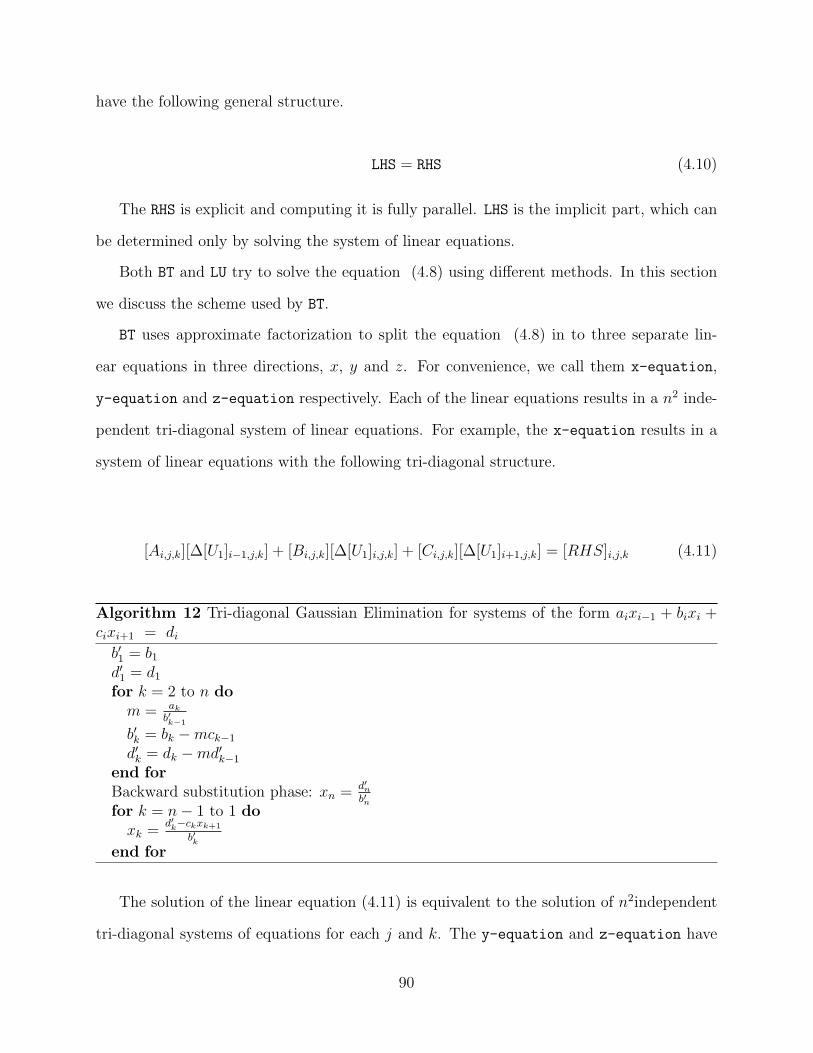
have the following general structure.
LHS = RHS (4.10)
The RHS is explicit and computing it is fully parallel. LHS is the implicit part, which can
be determined only by solving the system of linear equations.
Both BT and LU try to solve the equation (4.8) using different methods. In this section
we discuss the scheme used by BT.
BT uses approximate factorization to split the equation (4.8) in to three separate lin-
ear equations in three directions, x, y and z. For convenience, we call them x-equation,
y-equation and z-equation respectively. Each of the linear equations results in a n2 inde-
pendent tri-diagonal system of linear equations. For example, the x-equation results in a
system of linear equations with the following tri-diagonal structure.
[Ai,j,k][∆[U1]i−1,j,k] + [Bi,j,k][∆[U1]i,j,k] + [Ci,j,k][∆[U1]i+1,j,k] = [RHS]i,j,k (4.11)
Algorithm 12 Tri-diagonal Gaussian Elimination for systems of the form aixi−1 + bixi +cixi+1 = di
b′1 = b1
d′1 = d1
for k = 2 to n dom = ak
b′k−1
b′k = bk −mck−1
d′k = dk −md′k−1
end forBackward substitution phase: xn = d′n
b′nfor k = n− 1 to 1 do
xk =d′k−ckxk+1
b′kend for
The solution of the linear equation (4.11) is equivalent to the solution of n2independent
tri-diagonal systems of equations for each j and k. The y-equation and z-equation have
90
similar formulations. Each of the tri-diagonal systems are solved using a special form of Gaus-
sian elimination for tridiagonal matrices (Algorithm 12). This computes the n unknowns in
O(n) steps as opposed to the O(n3) steps of the original Gaussian elimination. In the Algo-
rithm, xi,∀i = 1..n is the set of unknowns. Ignoring the details of the algorithm, it can be
seen that the statements inside both the loops have recurrences, thus leading to global data
dependencies. Thus, the algorithm is sequential and offers no parallelism. However, solving
each of the n2 linear equations is completely independent and can be performed in parallel.
Henceforth, solving the equations arising from x-equation, y-equation and z-equation
will be called as x-sweep, y-sweep and z-sweep respectively. These sweeps consists of
the forward elimination phases - x-eliminate, y-eliminate and z-eliminate - and back
substitution phases - x-back substitute, y-back substitute and z-back substitute.
The computations can be summarized as follows:
• i) The original linear equation is factored in to three separate linear equations (x-equation,
y-equation and z-equation).
ii) Each of the 3 linear equations lead to multiple independent systems of linear equa-
tions, which is solved using the special form of Gaussian elimination (x-sweep, y-sweep
and z-sweep).
iii) During each sweep there is global dependence along that dimension, but the other
dimensions are completely independent. Thus, for example, all the elements of a given
yz plane can be processed in parallel during xsweep. Similarly, all the elements of xz
and xy planes can be processed in parallel during ysweep and zsweep respectively.
The above steps give rise to a simple parallelization strategy, where in the 3D domain is
split in to equal sub-domains and assigned to different processors. All the processors that
own a line i can participate in the ith stage of the recurrence. The flow of computation for
a simpler 2D case is shown in Figure 4.19(a). In each case, regions of the same color can be
operated at the same time. A one to one row-cyclic processor distribution will result in a
sub-optimal program as only a subset of processors will work at a given time, while the rest
91

ysweep
xsweep
(a)
3
3
(b)
2 3
2 1
1
1
2
Figure 4.19: (a) Flow of control in BT (b) Double cyclic mapping for optimal performance
will idle during this time. A better scheme is to assign several tiles to a processor following
a double-cyclic arrangement of processors, as shown in Figure 4.19(b). Such a mapping
ensures that during each sweep, all the processors are working in parallel.
Given this parallel formulation, it is very natural to adopt it to use tiles. The input
domain is represented using a HTA of rank 3 with double-cyclic distribution.
The x sweep section of the MATLAB-serial version of BT are shown in Figure 4.20(a).
In BT each of the elements of the grid U is a vector of size 5 and the elements of the co-
efficient matrix of the linear system of equations are matrices of size 5× 5. Thus, the scalar
multiplications and division in Algorithm 12 are replaced by matrix multiplication (*) and
inversion (\) respectively. x-eliminate and x-backsubstitute have the same meaning as
explained in an earlier paragraph. x-eliminate takes as its input the matrices lhs, U and
rhs. a, b, c and d are the matrices A, B and C and D shown in the equation (4.11). Due to
brevity, the formation of these matrices is not shown in detail.
Figure 4.20(b) shows the MATLAB+HTA version. Here the matrices lhs, U and rhs
are 3D HTAs. They are mapped according to the double-cyclic distribution function
discussed earlier. The outer for loop controls the iteration over tiles. During each iteration
a line of tiles (i.e., all tiles with a given i index) are selected. The function x-eliminate is
applied to each of the selected tiles. This function is the same as the one in the MATLAB-
serial version, except that now this function operates on a sub-array. The communication
statements in the last two lines of the outer loop copy the end regions to the next set of
tiles (i.e., those tiles that will be selected in the next iteration of the i loop). The other
92

function bt
...
[lhsc, rhs] = x-eliminate (rhs, u lhs);
rhs = x-back substitute (rhs, lhsc);
...
function [lhsc, rhs] = x-eliminate (rhs, u, lhs)
for k = 1:nz-2
for j = 1:ny-2
%form a, b & c (not shown here)
...
c(:,:,1) = b(:,:,1) \ c(:,:,1);
rhs(:,1,j,k) = b(:,:,1) \ rhs(:,1,j,k);
for i = 2:nx
rhs(mm,i,j,k) = rhs(mm,i,j,k) -
a(:, :,i) * rhs(:,i-1,j,k);
b(:, :, i) = b(:, :,i) -
a(:,:,i) * c(:, :, i-1);
c(:,:,i) = b(:,:,i) \ c(:,:,i);
rhs(:,i,j,k) = b(:,:,i) \ rhs(:,i,j,k);
end
lhsc(:, :, i, j, k) = c(:, :, i);
end
end
function [rhs] = x-backsubstitute (rhs, c)
for k = 1:nz-2
for j = 1:ny-2
for i=nx-1:-1:0
for m=1:BLOCK_SIZE
for n=1:BLOCK_SIZE
rhs(m,1+i,1+j,1+k) = rhs(m,1+i,1+j,1+k) ...
- c(m,n,i+1,j+1,k+1) .* rhs(n,i+2,j+1,k+1);
end
end
end
end
end (a)
function bt
....
for i=1:dx
[rhs, lhs] = map (@x-eliminate,
rhs{:,i,:,:},
u{:,i,:,:},
lhs{:,i,:,:},
i);
if( i < dx )
rhs{:,i+1,:,:}(:,1,2:sy-1,2:sz-1) =
rhs{:,i,:,:}(:,sx-1,2:sy-1,2:sz-1);
lhs{:,i+1,:,:}(:,1,2:sy-1,2:sz-1) =
lhs{:,i,:,:}(:,sx-1,2:sy-1,2:sz-1);
end
end
for i=dx:-1:1
rhs{:,i,:,:} = map (@x-backsubstitute,
rhs{:,i,:,:},
lhs{:,i,:,:});
if( i > 1 )
rhs{:,i-1,:,:}(:,sx,2:sy-1,2:sz-1) =
rhs{:,i,:,:}(:,2,2:sy-1,2:sz-1);
end
end
.... (b)
Figure 4.20: x-sweep section of BT (a) MATLAB-serial version (b) MATLAB+HTA version
for loop is similar to the first one, except that it proceeds in the reverse order and invokes
x-backsubstitute on each tile.
The main advantage of HTA for BT is the ability to define complex distribution like
double-cylcic very easily and select the row of tiles using the HTA selection operation. The
flow of computation is evident in the code. At the same time, the programmer has explicit
control over performance. For example, he can change the processor mapping scheme very
easily according to his needs. Also, the notion of processors is absent in the program; instead,
the programmer thinks in terms of tiles. This leads to very good global view program which
is also processor independent.
In contrast, the MPI version controls the flow of computation using synchronization.
93
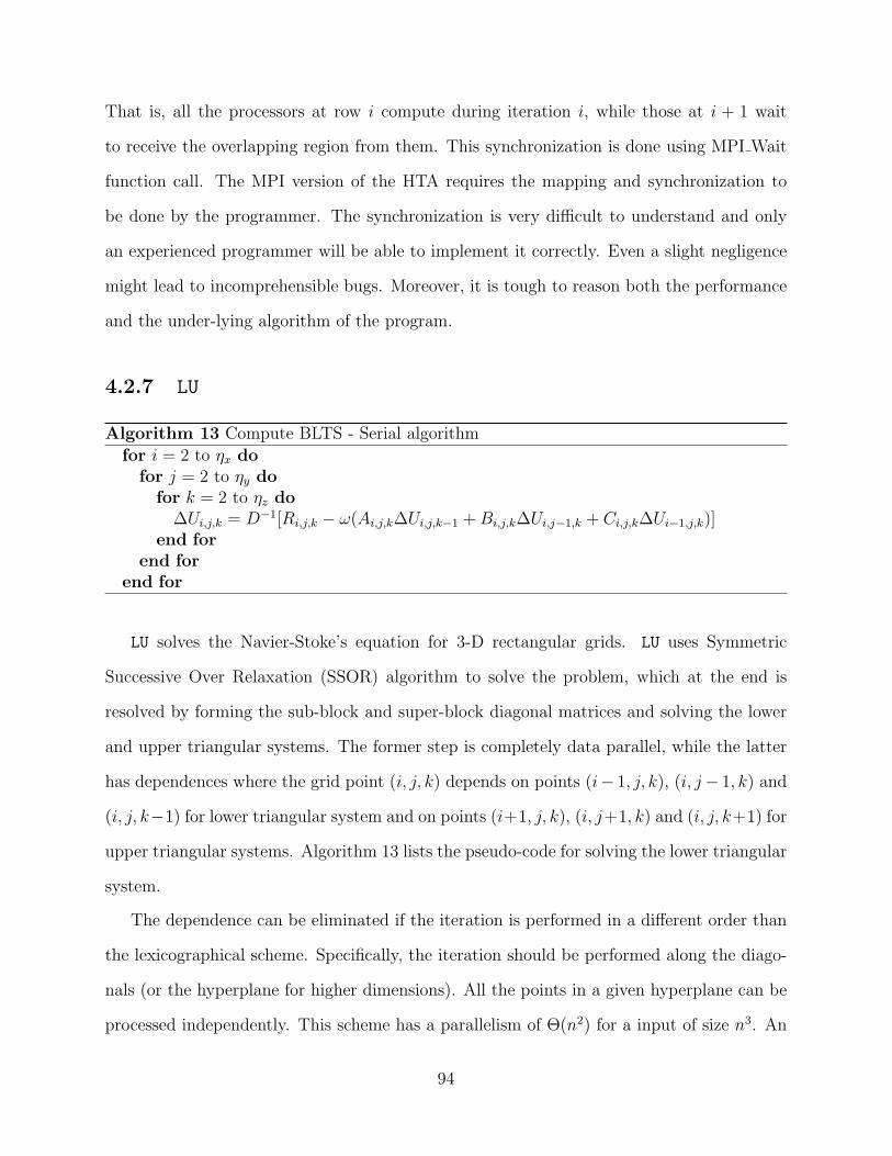
That is, all the processors at row i compute during iteration i, while those at i + 1 wait
to receive the overlapping region from them. This synchronization is done using MPI Wait
function call. The MPI version of the HTA requires the mapping and synchronization to
be done by the programmer. The synchronization is very difficult to understand and only
an experienced programmer will be able to implement it correctly. Even a slight negligence
might lead to incomprehensible bugs. Moreover, it is tough to reason both the performance
and the under-lying algorithm of the program.
4.2.7 LU
Algorithm 13 Compute BLTS - Serial algorithm
for i = 2 to ηx dofor j = 2 to ηy do
for k = 2 to ηz do∆Ui,j,k = D−1[Ri,j,k − ω(Ai,j,k∆Ui,j,k−1 + Bi,j,k∆Ui,j−1,k + Ci,j,k∆Ui−1,j,k)]
end forend for
end for
LU solves the Navier-Stoke’s equation for 3-D rectangular grids. LU uses Symmetric
Successive Over Relaxation (SSOR) algorithm to solve the problem, which at the end is
resolved by forming the sub-block and super-block diagonal matrices and solving the lower
and upper triangular systems. The former step is completely data parallel, while the latter
has dependences where the grid point (i, j, k) depends on points (i− 1, j, k), (i, j− 1, k) and
(i, j, k−1) for lower triangular system and on points (i+1, j, k), (i, j+1, k) and (i, j, k+1) for
upper triangular systems. Algorithm 13 lists the pseudo-code for solving the lower triangular
system.
The dependence can be eliminated if the iteration is performed in a different order than
the lexicographical scheme. Specifically, the iteration should be performed along the diago-
nals (or the hyperplane for higher dimensions). All the points in a given hyperplane can be
processed independently. This scheme has a parallelism of Θ(n2) for a input of size n3. An
94

(b)(a)
Figure 4.21: Hyperplane
example hyperplane of a n × n × n matrix is shown in the Figure 4.21(a). Figure 4.21(a)
shows the hyperplane iteration over scalars, while Figure 4.21(b) shows the iteration over
tiles. In the figure, all the elements (scalars or tiles) of the same color can be processed in
parallel.
Algorithm 14 Compute BLTS - Hyperplane algorithm
define sets Hm = {(i, j, k)|i + j + k = m}, m = 6, 7, ... (ηx + ηy + ηz − 3)for m = 6 to (ηx + ηy + ηz − 3) do
for all (i, j, k) ∈ Hm do∆Ui,j,k = D−1[Ri,j,k − ω(Ai,j,k∆Ui,j,k−1 + Bi,j,k∆Ui,j−1,k + Ci,j,k∆Ui−1,j,k)]
end forend for
Algorithm 14 shows the wavefront algorithm for parallelizing a section of the LU bench-
marks, namely the solution of the block lower triangular system (blts). Using the hyperplane
scheme, the processors compute local data before sending them to the processors containing
the dependent data.
The hyperplane scheme can be implemented using HTA, where the iteration proceeds
over tiles, as shown in Figure 4.22. The figure illustrates the hyper-plane scheme for a 2-
dimensional case. To control the iteration, the logical indexing is used to determine the
tiles that can operate in each iteration of the K loop. The expression I+J==K composes
a boolean array. Tiles with true value in the boolean array will be selected to do the 2D
wavefront computation. The last two statements in Figure 4.22(b) copy the last row and
column of the tiles of the K-th diagonal to the first row and column of the corresponding tiles
95

for i=2:m-1
for j=2:n-1
A(i, j) = A(i-1, j) + A(i, j-1);
end
end (a)
for k = 2:m+n
for i=2:dimx-1
for j = 2:dimy-1
A{x+y == k}(i, j) = A{x+y==k}(i-1, j)+
A{x+y==k}(i, j-1);
end
end
A{x+y == k+1 & x > 1}(1, :) =
A{x+y == k & x < m}(dimx-1, :);
A{x+y == k+1 & y > 1}(:, 1) =
A{x+y == k & y < n}(:, dimy-1);
end (b)
2
33
2
3
1 12
3
211
21
1
2 3
2
3
3
44
4
1x = y =
(c)
Figure 4.22: Forward phase of a simple SSOR iteration a) Using MATLAB serial programb) Using MATLAB HTA program c) Illustration of the diagonal iteration over the tiles
in the K+1-th diagonal. This is done to update the shadow of these tiles which guarantee
that all the data needed for each computation is in the same tile.
A pictorial view of how the computation advances across tiles is shown in Figure 4.22(c),
where the values of the I and J matrices are also shown. In the Figure, a is a M ×N HTA,
distributed on a M × 1 processor mesh, so that each row of tiles is mapped to the same
processor. In the LU program, data are partitioned into M × N ×K tiles, and distributed
across M ×N processors, so that the third dimension is local to each processor.
Implementation of this scheme using FORTRAN+MPI is extremely cumbersome. Unlike
the other benchmarks, the processors do not execute in perfect synchronization. Rather,
there is a producer consumer relationship between the processors, where one group acts as
producer and another as consumers. This can be realized using careful synchronization of
the processors, by appropriately placing the MPI Send and MPI Recv function calls. Misuse
of this might lead to a deadlock. Moreover, it is very difficult to debug parallel programs
96
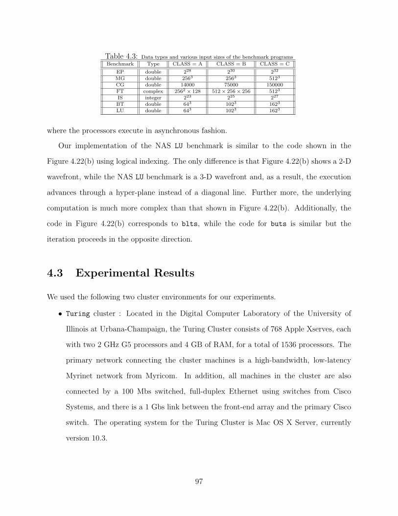
Table 4.3: Data types and various input sizes of the benchmark programs
Benchmark Type CLASS = A CLASS = B CLASS = C
EP double 228 230 232
MG double 2563 2563 5123
CG double 14000 75000 150000FT complex 2562 × 128 512× 256× 256 5123
IS integer 223 225 227
BT double 643 1023 1623
LU double 643 1023 1623
where the processors execute in asynchronous fashion.
Our implementation of the NAS LU benchmark is similar to the code shown in the
Figure 4.22(b) using logical indexing. The only difference is that Figure 4.22(b) shows a 2-D
wavefront, while the NAS LU benchmark is a 3-D wavefront and, as a result, the execution
advances through a hyper-plane instead of a diagonal line. Further more, the underlying
computation is much more complex than that shown in Figure 4.22(b). Additionally, the
code in Figure 4.22(b) corresponds to blts, while the code for buts is similar but the
iteration proceeds in the opposite direction.
4.3 Experimental Results
We used the following two cluster environments for our experiments.
• Turing cluster : Located in the Digital Computer Laboratory of the University of
Illinois at Urbana-Champaign, the Turing Cluster consists of 768 Apple Xserves, each
with two 2 GHz G5 processors and 4 GB of RAM, for a total of 1536 processors. The
primary network connecting the cluster machines is a high-bandwidth, low-latency
Myrinet network from Myricom. In addition, all machines in the cluster are also
connected by a 100 Mbs switched, full-duplex Ethernet using switches from Cisco
Systems, and there is a 1 Gbs link between the front-end array and the primary Cisco
switch. The operating system for the Turing Cluster is Mac OS X Server, currently
version 10.3.
97

Table 4.4: Configuration of the experimental environments.
Specifications Turing cluster Tungsten cluster
Processors 2 GHz G5 Intel Xeon 3.2 GHzOperation System Max OS X server Linux
Memory/Node 4 GB 3 GBInterconnet Myrinet/Gigabit Ethernet Myrniet/Gigabit EthernetMPI Library mpich-gm Champion/Pro MPI
Compiler GNU N/A
Table 4.5: Tiling structure and processor distribution.
Benchmark Shape of the HTA Processor Distribution
EP {1, [p]} 1-to-1 row-cyclicMG {3, [m× n× k]}, mnk = p 1-to-1 row-cyclicCG {2, [m× n]}, mn = p 1-to-1 row-cyclicFT {3, [p× 1× 1]} 1-to-1 row-cyclicIS {1, ([p], [p])} 1-to-1 row-cyclicBT {3, [m× n× k]}, mn = p k-to-1 double-cyclicLU {3, [m× n× k]}, mn = p k-to-1 row-cyclic
• Tungsten cluster : Tungsten cluster is a linux cluster of 32 bit Intel Xeon (3.2 GHz)
processors. The number of compute nodes is 1280. The cluster is located in the
National Center for Super Computing Applications (NCSA), University of Illinois at
Urbana-Champaign. The nodes are connected via myrinet and gigabit Ethernet. Each
node has a RAM of 3 GB and a disk memory of 70 GB.
The NAS benchmark programs can be compiled for various input sizes. These input sizes
are known as classes. The input sizes of each class of the benchmark programs are listed in
4.3.
Table 4.5 lists the shape and the processor distribution (cf Section 2.1.2) of the HTA
programs. The F77+MPI also use identical processor distribution. In the table, x− to− y
represents the number of tiles (x) mapped to number of processors (y). p is the total number
of processors and m, n, k are integers. Except BT, all the programs run only with number
of processors which is a power of two. Except FT and IS, all the programs use one level of
tiling. IS uses two-level tiling for reasons mentioned in Section 4.2.5. The MATLAB+HTA
version of FT uses one level of tiling, while the CPP+HTA version uses two levels of tiling.
This is used only for performance reasons. By using a two level tiling, the programmer can
control the granularity of communication during the dtranspose operation.
98

Before proceeding to the analysis of our results, the readers are advised to take into
consideration the following issues to appreciate the results that we have obtained so far.
• All the programs were written from scratch manually following the algorithms pub-
lished in the NAS benchmark program report [7]. For MATLAB, we implemented
both the serial and the parallel versions. The serial programs were required because
the MATLAB programs were the first to be written in HTA. Without an understand-
ing of the serial programs, it is very difficult to write the HTA programs. Moreover,
we demonstrated that it is easy to convert existing sequential MATLAB programs to
parallel HTA programs, through this step.
• Our goal in these experiments is not to outperform the F77+MPI programs. Rather,
we like to show that with appropriate implementation and proper tuning, HTA pro-
grams can scale as well as F77+MPI programs. By aggressive manual tuning of both
the library and the HTA source programs, it may be possible to even outperform
the F77+MPI programs. In fact, we have observed such outstanding performance in
certain cases. We also have identified several optimizations difficult to program in
F77+MPI, but are easy for HTA programs. Yet, instead of restricting ourselves to
tuning a single program and outperform the F77+MPI, we implemented an almost
complete set of NAS benchmarks. The key reason for this decision is to analyze a
diverse set of benchmarks and study the suitability of HTA as a programming model
for a wide range of programs and on large number of processors.
• We require 128 licenses of MATLAB, if we need to conduct our experiments in 128
processors. In the Tungsten cluster, where we ran all our experiments, we were provided
the licenses only for a short duration (1 month). This restricted our program tuning
and performance behavior understanding efforts drastically.
• Each of the NAS program is different and unique in the computation and communica-
tion. The programs offer various challenges like load balancing, optimal communica-
99

tion, irregular problem domains, to name a few. The performance behavior of each of
the program is different.
• We do not have any sophisticated compiler to perform any source code optimization
of the HTA programs. For C++, the compilers perform traditional scalar optimiza-
tions. But, for MATLAB, even a traditional optimizations like common sub expression
elimination, are performed manually. Some of the manual optimizations we performed
for the HTA programs are pre-allocation of temporary HTAs for the entire program,
conversion of data parallel operations to map operations and removal of loop-invariant
tile access operations (h()).
• F77+MPI programs have been tested, optimized and rewritten for over a decade. They
were developed professionally at a scientific laboratory (NASA) by several scientists.
4.3.1 MATLAB Library
For the MATLAB library, we performed our experiments in the Tungsten cluster. The raw
running times of the programs up to 128 processors is given in Table 4.6.
The execution time for 1 processor corresponds to the serial execution of the pure F77
or MATLAB code without MPI or HTAs, depending of the base. Results in Table 4.6
correspond to the class C input for EP and CG, and class B for MG, FT, LU and BT. Table 4.7
shows the ratio of MATLAB+HTA and F77+MPI programs.
One of the key challenges we faced in writing the MATLAB+HTA programs is to write
optimal MATLAB programs. MATLAB programs should adhere to certain rules for optimal
efficiency. For example, vectorization of programs is an important requirement for efficiency.
The key reason for MATLAB being interpreted is that it uses array computations intensively.
Interpreting costs are amortized by using such array operations. The array operations are
executed efficiently by a compiled library code. Using non-vectorized scalar codes is counter
intuitive in MATLAB. So, all our MATLAB programs are aggressively vectorized. However,
100

Tab
le4.
6:E
xec
ution
tim
esin
seco
nds
for
som
eof
the
applica
tions
inth
eN
AS
ben
chm
ark
sfo
rF77+
MP
Iver
sus
MAT
LA
B+
HTA
.T
he
exec
ution
tim
efo
r1
pro
cess
or
corr
esponds
toth
ese
rialapplica
tion
inF77
or
MAT
LA
B,w
ithout
MP
Ior
HTA
s.T
he
exec
uti
on
envir
onm
ent
isth
eTungsten
clust
er.
Npro
csE
P(
C)
FT
(B
)C
G(
C)
MG
(B
)LU
(B
)N
pro
csB
T(B
)F77+
Matl
ab
+F77
+M
atl
ab
+F77
+M
atl
ab
+F77
+M
atl
ab
+F77
+M
atl
ab
+F77
+M
atl
ab
+M
PI
HTA
MP
IH
TA
MP
IH
TA
MP
IH
TA
MP
IH
TA
MP
IH
TA
1901.6
3556.9
136.8
657.4
3606.9
3812.0
26.9
828.0
15.7
245.1
113.7
81543.1
14
273.1
888.8
109.1
274.0
362.0
1750.9
17.0
273.8
6.3
60.5
45.1
9570.5
28
136.3
447.0
65.5
159.3
123.4
823.6
9.6
151.3
2.9
29.9
92.5
6243.8
316
68.6
224.8
37.2
87.2
89.5
375.2
4.8
87.0
1.2
16.0
25
1.1
295.9
732
34.7
112.0
20.7
42.9
48.4
250.3
3.3
54.9
1.1
9.8
49
0.7
256.7
964
17.1
56.7
10.4
24.0
44.5
148.0
1.6
50.4
1.3
7.1
81
0.5
729.3
8128
8.5
29.1
5.9
15.6
30.8
123.0
1.4
38.5
1.6
N/A
100
0.5
44.5
7
101
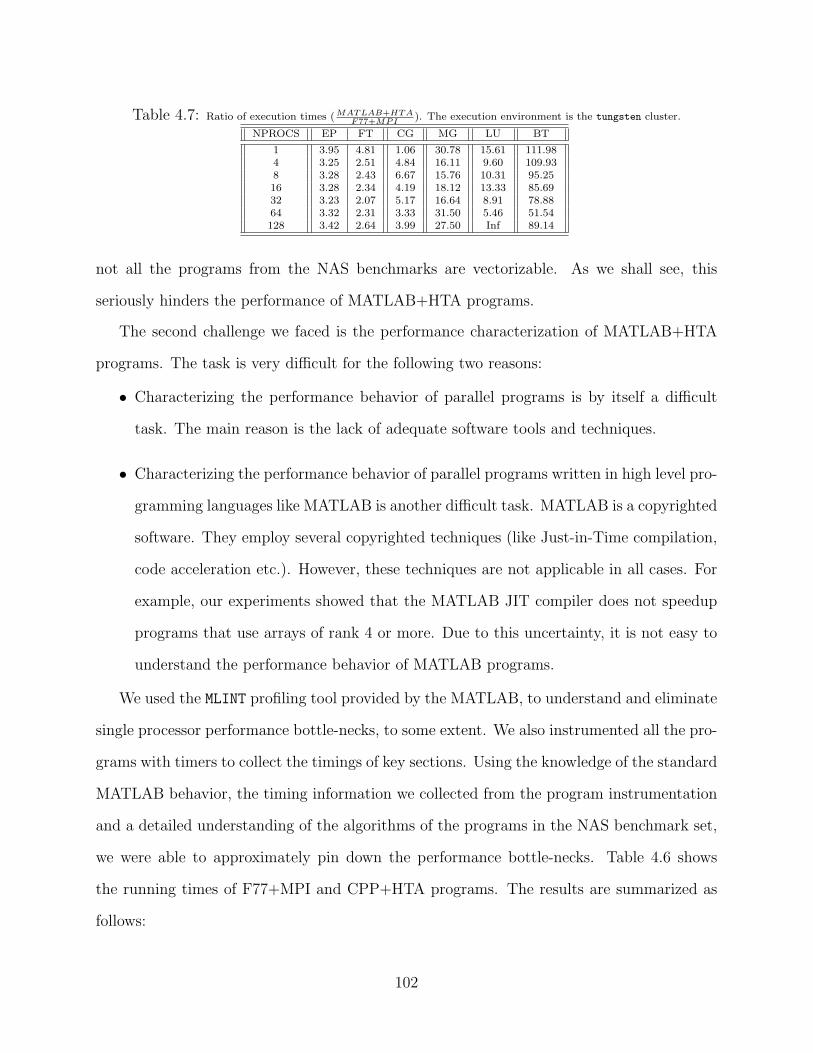
Table 4.7: Ratio of execution times (MATLAB+HTAF77+MPI
). The execution environment is the tungsten cluster.
NPROCS EP FT CG MG LU BT
1 3.95 4.81 1.06 30.78 15.61 111.984 3.25 2.51 4.84 16.11 9.60 109.938 3.28 2.43 6.67 15.76 10.31 95.2516 3.28 2.34 4.19 18.12 13.33 85.6932 3.23 2.07 5.17 16.64 8.91 78.8864 3.32 2.31 3.33 31.50 5.46 51.54128 3.42 2.64 3.99 27.50 Inf 89.14
not all the programs from the NAS benchmarks are vectorizable. As we shall see, this
seriously hinders the performance of MATLAB+HTA programs.
The second challenge we faced is the performance characterization of MATLAB+HTA
programs. The task is very difficult for the following two reasons:
• Characterizing the performance behavior of parallel programs is by itself a difficult
task. The main reason is the lack of adequate software tools and techniques.
• Characterizing the performance behavior of parallel programs written in high level pro-
gramming languages like MATLAB is another difficult task. MATLAB is a copyrighted
software. They employ several copyrighted techniques (like Just-in-Time compilation,
code acceleration etc.). However, these techniques are not applicable in all cases. For
example, our experiments showed that the MATLAB JIT compiler does not speedup
programs that use arrays of rank 4 or more. Due to this uncertainty, it is not easy to
understand the performance behavior of MATLAB programs.
We used the MLINT profiling tool provided by the MATLAB, to understand and eliminate
single processor performance bottle-necks, to some extent. We also instrumented all the pro-
grams with timers to collect the timings of key sections. Using the knowledge of the standard
MATLAB behavior, the timing information we collected from the program instrumentation
and a detailed understanding of the algorithms of the programs in the NAS benchmark set,
we were able to approximately pin down the performance bottle-necks. Table 4.6 shows
the running times of F77+MPI and CPP+HTA programs. The results are summarized as
follows:
102
EP
For the experiments, we use the map version of EP, shown in the Figure 4.3. The running
time of the MATLAB+HTA programs are around 4 times slower than that of the F77+MPI
programs. The main reason is that the for loop in Figure 4.3 runs for a total of 216 iterations
for CLASS C. Loops slow down the MATLAB programs by a significant factor. The other
reason for slow down is the creation of intermediate temporary array variables (x1, x2, xt1,
etc). However, the speedup of the MATLAB+HTA and F77+MPI programs are very similar.
MG
The performance of MG MATLAB+HTA programs is around 30 times higher than that of
F77+MPI programs. A visual inspection of the Table 4.6 reveals that 128 processor execu-
tion of MATLAB+HTA programs is slower than single processor execution of the F77+MPI
program. The main problem in MG is the excessive creation of the temporary arrays dur-
ing stencil computations. The stencil computation in MG involves 27 neighbors. When this
stencil computation is implemented as an array operation, 27 intermediate arrays are cre-
ated. This causes several overheads: increased usage of main memory, capacity misses in
the caches and management of these temporary arrays by the MATLAB run-time environ-
ment. Though, MATLAB provides an optimized function (imfilter) call to implement this
stencil convolution, we did not use this in the experiments we have reported here. In other
experiments, usage of imfilter improved the execution time of MATLAB+HTA programs
by a factor of two. The reason for not using imfilter is to use HTAs for implementing all
the primitive operations as much as possible.
FT
The MATLAB+HTA programs are on an average 3 times slower than that of F77+MPI
programs. The reasons for this are the standard MATLAB overheads : presence of loops,
interpretation overheads and creation of temporaries. Since, the major part of the FT pro-
103
gram is spent in the MATLAB ft routine (which in turn uses the FFTW [30] [29] library),
the slowdown is not too high. The scaling is also similar to that of the F77+MPI programs.
CG
For CG, F77+MPI programs exhibit super-linear speedups. We suspect that the reason is
the high activity of virtual memory swapping for small number of processors (1 and 4) in
F77+MPI program. On the other hand, MATLAB+HTA programs always consume more
memory and this swapping may be uniform for all the processor configurations. The other
standard MATLAB overheads hold for the CG program also.
LU
The execution times of LU is around 10 times that of F77+MPI. The reason for this gap
in LU is that it is not a vectorizable programs. It may be recalled from the description of
LU that it has global data dependences, owing to first order linear recurrence. Though, we
obtain parallelism using hyperplane iteration over the tiles, inside each tile we evaluate each
of the elements in lexicographic order, leading to strict sequential execution. Non-vectorized
programs do not deliver optimal performance in MATLAB.
BT
The execution times of BT is around 50 times slower than that of F77+MPI. Owing to large
execution times of MATLAB+HTA programs, we ran the BT program only for a small number
of iterations (5), instead of executing the program till completion. The reasons that hold
for LU also hold for BT, namely the first order linear recurrence prohibits the vectorization
of computations within a tile.
104

Tab
le4.
8:E
xec
uti
on
tim
esin
seco
nds
for
pro
gra
ms
inth
eN
AS
ben
chm
ark
sfo
rF77+
MP
Iand
CP
P+
HTA
.T
he
exec
uti
on
envir
onm
ent
isth
eturing
clust
er.
Input
size
for
LU
isC
LA
SS
A.For
all
oth
ers,
itis
class
C.
Npro
csE
P(C
)FT
(C)
CG
(C)
MG
(C)
IS(C
)LU
(A)
F77
+C
PP
+F77
+C
PP
+F77
+C
PP
+F77
+C
PP
+F77
+C
PP
+F77
+C
PP
+M
PI
HTA
MP
IH
TA
MP
IH
TA
MP
IH
TA
MP
IH
TA
MP
IH
TA
11329.1
31532.7
0–
–4632.6
76239.8
4–
––
–253.0
1597.6
82
762.7
7880.7
2–
–1190.7
31280.4
7161.6
9–
21.3
3–
126.7
9390.1
24
381.6
2442.3
8720.1
0664.9
6746.9
3648.5
193.0
983.0
012.8
023.7
162.0
4239.2
08
190.6
4220.4
0337.3
2345.2
0209.5
6424.3
138.4
545.1
17.6
113.9
229.6
1124.0
316
95.3
9110.3
6173.4
8175.6
5121.5
8170.4
722.5
424.1
25.3
68.4
413.0
474.7
32
47.7
155.3
6142.4
595.6
446.7
982.6
212.4
412.9
03.8
15.8
28.6
738.7
164
23.8
528.3
146.4
356.6
032.4
752.1
55.3
67.6
52.8
03.9
54.2
327.2
2128
11.9
314.1
420.4
331.5
917.2
726.8
73.4
55.3
91.8
23.0
82.4
0–
105

Table 4.9: Ratio of execution times (CPP+HTAF77+MPI
). The execution environment is the turing cluster. Input size for LU is
CLASS A. For all others, it is class C.
NPROCS EP FT CG MG IS LU
1 1.15 – 1.35 – – 2.362 1.15 – 1.08 – – 3.084 1.16 0.92 0.87 0.89 1.85 3.868 1.16 1.02 2.02 1.17 1.83 4.1916 1.16 1.01 1.40 1.07 1.57 5.7332 1.16 0.67 1.77 1.04 1.53 4.4664 1.19 1.22 1.61 1.43 1.41 6.43128 1.19 1.55 1.56 1.56 1.69 –
Figure 4.23: Running time comparison of F77+MPI and CPP+HTA on Turing cluster : EPBenchmark (Class C)
4.3.2 C++ Library
We executed the CPP+HTA programs in the Turing cluster. We used g77 and g++ compil-
ers for compiling the FORTRAN and C++ programs respectively. For both the programs,
we used the mpichgm library, an MPI implementation for Myrinet. The running times
of the programs are shown in Table 4.8, while Table 4.9 shows the ratio of CPP+HTA
and F77+MPI running times. Figures 4.23– 4.28 show the plot of running times of the
CPP+HTA programs and F77+MPI programs. For all the programs, except LU, we used
CLASS C as the input size. For LU, we used CLASS A as the input size.
106
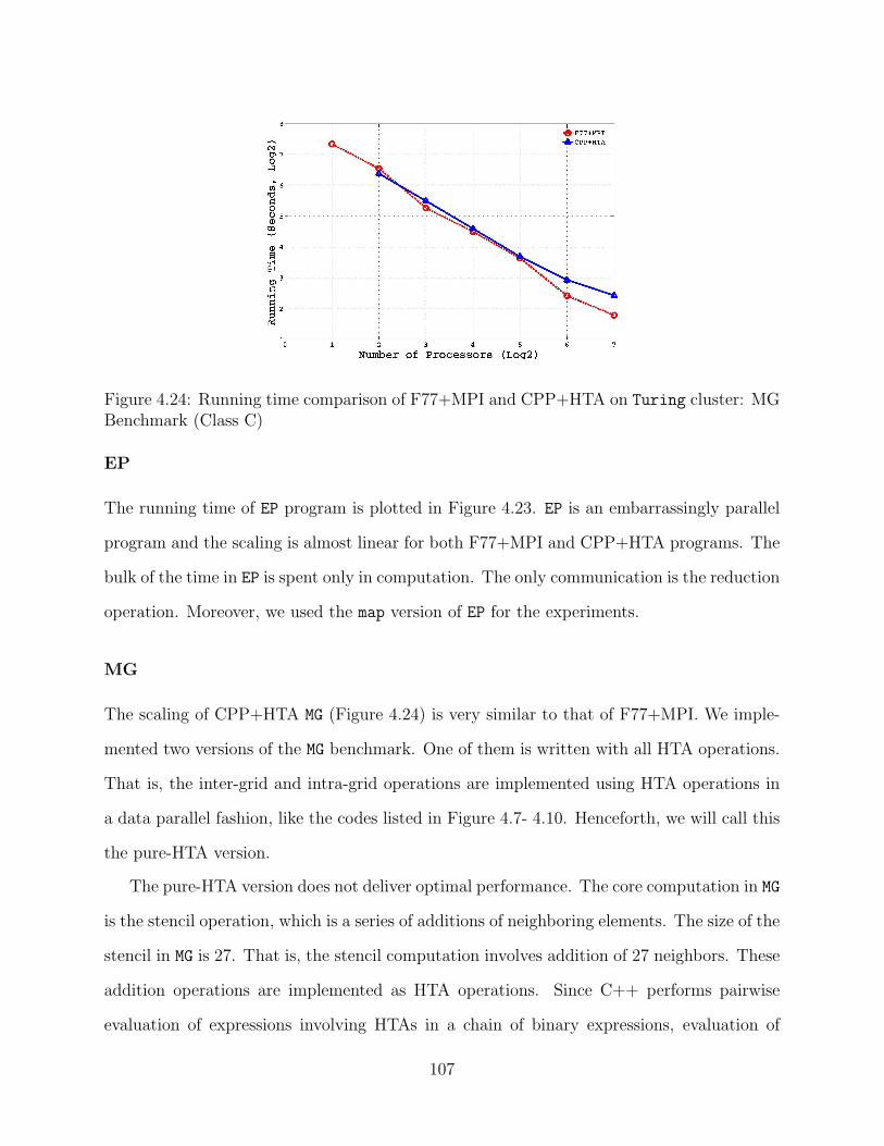
Figure 4.24: Running time comparison of F77+MPI and CPP+HTA on Turing cluster: MGBenchmark (Class C)
EP
The running time of EP program is plotted in Figure 4.23. EP is an embarrassingly parallel
program and the scaling is almost linear for both F77+MPI and CPP+HTA programs. The
bulk of the time in EP is spent only in computation. The only communication is the reduction
operation. Moreover, we used the map version of EP for the experiments.
MG
The scaling of CPP+HTA MG (Figure 4.24) is very similar to that of F77+MPI. We imple-
mented two versions of the MG benchmark. One of them is written with all HTA operations.
That is, the inter-grid and intra-grid operations are implemented using HTA operations in
a data parallel fashion, like the codes listed in Figure 4.7- 4.10. Henceforth, we will call this
the pure-HTA version.
The pure-HTA version does not deliver optimal performance. The core computation in MG
is the stencil operation, which is a series of additions of neighboring elements. The size of the
stencil in MG is 27. That is, the stencil computation involves addition of 27 neighbors. These
addition operations are implemented as HTA operations. Since C++ performs pairwise
evaluation of expressions involving HTAs in a chain of binary expressions, evaluation of
107

Table 4.10: Comparison of running times (seconds) of pure-HTA and map versions of MG (CLASS C) in turing cluster.
Processors map version pure-HTA version
4 83.00 –8 45.11 884.9416 24.12 410.7232 12.90 215.8564 7.65 110.66128 5.39 67.11
each of the addition operation produces a temporary. The creation of temporary might
cause capacity misses in cache and other levels of memory hierarchy. In such a pairwise
evaluation, each evaluation is a function call (for e.g. operator +). Finally, the body of
the function, which often contains a loop that iterates over all the elements of its inputs, is
executed several times, thus leading to more loop instructions being executed.
We avoided the creation of temporaries during stencil operation using an optimized lconv
(acronym for leaf convolution) routine that is invoked via map on the input HTAs. The
lconv performs the stencil operation on an array. In the case of HTA programs, the lconv
is invoked on each of the leaf tiles of the HTAs, using hmap operation. The map version of MG
runs up to 20 times faster than the pure-HTA version(see Table 4.10). We used this version
for our experiments in Figure 4.24. The process of converting the HTA operations in to a
map operation automatically using a compiler, is a future work.
The problem of temporaries can also be avoided by using delayed expression evaluation
technique. In this technique, the evaluation of a chain of expression is delayed until its use
(i.e., an assignment operation). Inside the assignment operation, the expression is evaluated
as a whole in to the left hand side argument. Thus, no temporaries are created and all the
expressions are evaluated and assigned in a single loop. This technique can be implemented
at run-time (using proxy objects) or compile-time (using expression templates [49]). We have
implemented a simple run-time scheme only for binary expressions (in the context of CG).
Extending this scheme to a chain of binary expressions or implementing the compile-time
scheme using expression templates remains to be done.
108

Figure 4.25: Running time comparison of F77+MPI and CPP+HTA on Turing cluster: CGBenchmark (Class C)
CG
The running time plot of CG is shown in Figure 4.25. As can be seen in the graph, the running
times of CPP+HTA version is within a factor of 1.5 (on average) of that of F77+MPI version.
The scaling pattern of both the versions are very similar.
The core computation in CG is a sparse matrix-vector multiplication. F77+MPI version
uses compressed column storage layout for the sparse matrix, while the CPP+HTA programs
use compressed row storage.
For the CPP+HTA version we use different programs depending on the parity of the
logarithm of the number of processors. If the number of processors is an even power of two,
then we use a square HTA (i.e., the number of elements along both the dimensions are the
same). If the number of processor is an odd power of two, then there are two choices for HTA
structure – rectangular and square. If square HTAs are used, two tiles need to be mapped
to a given processor. Using such a distribution in the CG program listed in Section 4.2.3
does not deliver optimal performance. The CG algorithm requires replication of vectors and
hence replication of computations, and this replication happens on a per-tile basis. If two
tiles are mapped to a processor, a tile could be replicated twice on a same processor. This in
turn results in certain computations (e.g. the pT q step), to be redundantly executed twice.
109

Figure 4.26: Running time comparison of F77+MPI and CPP+HTA on Turing Cluster :FT Benchmark (Class C)
Moreover, during operations like reduce and transpose, which involve communication,
twice the messages than the required will be exchanged between processors. For these
reasons, we use a rectangular HTAs. This in turn requires some changes to the matrix-
vector multiplication part of the CG program. The F77+MPI version uses a single program
for both the cases with extra logic to handle the rectangular cases.
As a future work, a modified form of the HTA repmat operation is under-study. This
operation will not duplicate an element in the same processor. Instead all the instances of
that element in a given processor will point to a single unique instance. This will avoid the
creation of two separate programs.
FT
The running times of the FT CPP+HTA version is within a factor of 1.5 of that of the
F77+MPI version (Figure 4.26). Until 32 processors, the performance is very close to
F77+MPI, with 4 and 8 processor execution beating the F77+MPI version slightly.
Unlike in MATLAB, we do not use any optimized Fourier transform library like FFTW,
for the CPP+HTA version. Instead, we use the same Fourier transform routine that the
F77+MPI programs use. The scaling of CPP+HTA programs is also very similar to that of
110
the F77+MPI programs up to 64 processors.
The F77+MPI version distributes the array along the third dimension. This is optimal for
F77+MPI programs, as FORTRAN assume column major storage layout for all its arrays.
During the transposition step, the first and the third dimension are exchanged and this
involves a copy of values. The Fourier transform is applied twice along the first dimension
and once along the second dimension. For better cache utilization, all the elements of a
vector stored in non-contiguous memory regions are copied to consecutive locations, before
performing the Fourier transform. This implies that whenever the transform is applied along
the second dimension, a copy operation is performed. Thus, totally two copies are required
for computing the Fourier transform along all the dimensions. Since C++ and the htalib use
row major storage layout for the arrays, we distribute the HTAs along the first dimension,
to ensure the same optimal two copy requirement.
Additionally, in the CPP+HTA version we use an HTA of height two, instead of HTA
of height one of our earlier MATLAB+HTA version. The transposition operation (refer
Section 4.2.4) involves an all-to-all exchange of data between processors, if the HTA is
distributed. By using a 2-level tiling, the programmer can control the size of the message
and the number of messages exchanged during this communication step.
F77+MPI uses blocked transposition and FFT computation. Since, the HTA program
is not written that way, for the experiments, we set the block size to be one for F77+MPI
program. To incorporate the block transposition and FFT computation, we need to add one
or more level of tiling. This is left as a future work.
IS
IS program of NAS benchmark set is written in C, unlike the other programs. The running
time of IS (Figure 4.27) CPP+HTA is within a factor of 1.414 of that of F77+MPI programs.
The scaling patterns for both the programs are very similar.
111

Figure 4.27: Running time comparison of C+MPI and CPP+HTA on Turing cluster: ISBenchmark (Class C)
LU
The single processor running time of LU-CPP+HTA version (Figure 4.28) is only a factor of
2 times higher than that of F77+MPI. In LU the main single processor overhead is the usage
of operator[] (flat operator). LU uses map operation to implement all its core computation
(blts, buts and rhs). Inside these functions, operator[] is used very frequently to iterate
over the individual scalar functions. The main computation of operator[] (i.e., the index
arithmetic) is not translated optimally by the C++ compiler we used. Certain optimizations
like loop invariant index arithmetic operations removal, common sub-expressions elimination
and strength reduction are not performed by the compiler. This leads to the slowdown by a
factor of 2.34 for the single processor execution.
The main multi processor overhead is the excessive usage of operator (). In LU, the
chained tile access operation (like, h(r00, r0
1)[r10, r1
1], where each rji is a range), is called very
frequently to exchange the neighboring data (See Figure 4.22(b)). The cost of a single h(r00,
r01)[r
10, r1
1] operation is O(t), where t is the number of elements in the region (r00, r0
1).
The HTA version of LU uses the hyperplane algorithm [9]. The outer time step loop
iterates for a large number of times (e.g. 250 iterations for CLASS A). Inside each time
step, there is an iteration over each of the hyperplanes of the HTA. The total number of
112

Figure 4.28: Running time comparison of F77+MPI and CPP+HTA on Turing cluster: LUBenchmark (Class A)
hyperplanes is O(√
p), where p is the number of processors. For each hyperplane iteration,
the chained access operation is invoked. There are two separate hyperplane iterations, one
for blts and another for buts. During each hyperplane iteration the communication method
to exchange the neighboring data is called. Thus, the total number chained access operation
invocations is 2 × 250 × O(√
p) = O(√
p). Further, the number of tiles is chosen to be
O(p√
p), for optimal performance. Putting all together, the total cost of the chain access
operation is O(p2). Thus, the overhead increases by a quadratic factor of the number of
processors.
We eliminated this overhead by memorizing the intermediate HTAs generated during the
hyperplane iterations in an array of temporaries. These temporary HTAs are used inside
the communication step. Since, the htalib provides a mechanism to generate different views
of an HTA that share the same under-lying data, this optimization is possible. A compiler
can pre-compute all the HTA that result after the chained access operations. For example,
in h(r00, r0
1)[r10, r1
1], if the ranges rji are loop-invariant, the chained access operation can be
computed outside of the loop resulting in a temporary HTA. The access operation itself will
be replaced by these temporary HTAs. Yet another solution to the problem is the usage
of overlapped tiling [35], which will eliminate the need to use the chained access operation
113

during communication.
4.3.3 Summary
The re-writing of the NAS benchmarks and the implementation of the HTA library in C++
provided adequate platform to understand the performance behavior of HTA programs.
Our earlier MATLAB implementation was constrained by the larger execution times of
MATLAB programs. Unless the execution times are very close to a compiled and optimized
FORTRAN77 or C program, the speedups obtained are not legitimate. Thus, the results
from the C++ library is more representative of the HTA program performance than the
MATLAB library.
With the current maturity level of the C++ library, we observed a slowdown of up to a
factor of 2.5 for the CPP+HTA programs (on a single processor execution) compared with
F77+MPI programs. It can be seen from the Table 4.9 that the slowdown is not uniform
for all the programs. For LU, the factor is over two, while EP, MG FT, CG and IS have a lesser
factor (≈ 1.5).
We identified several overheads in each benchmark program. The most common overhead
in all the programs is the creation of temporary HTAs. This is an inherent drawback of
any data-parallel language. An aggressive compiler or a technique like delayed expression
evaluation will solve this problem. At present, we avoided this problem, in most cases, by the
usage of map operation or pre-allocation of temporaries. Yet, there are few more temporaries
that are created inside the HTA operations at run-time. For example, in FT, the dtranspose
operation creates two buffers while transposing the input HTA h. In a F77 program, only one
temporary is allocated once for the entire program and is re-used during each transposition
step. The creation of temporaries lead to capacity misses and runtime overhead involved
in managing them. Another common overhead is the inability of the compiler to generate
the optimal code for operator [] (scalar selection). We discovered that the compiler does
not perform loop-invariant removal and strength reduction. In MG, we avoided the usage of
114

operator[] by hand translating the operator[] to the index arithmetic computation. In LU,
we did not do this and hence slowdown by a factor of 2.3.
The two-sided communication method of the htalib has several undesirable effects on
the performance of HTA programs. The HTA meta-data needs to be replicated in all the
processors, so that in an HTA operation a processor knows its partner. As the number
of processors increases the size of the HTA meta-data also increases proportionally. Thus,
for large number of processors the memory consumption of HTA programs could increase
drastically. This might limit the scalability of the HTA programs as the number of pro-
cessors increases. To solve this, the library has to be re-engineered to use one-sided put
and get operations. Additionally, the two-sided communication might lead to unnecessary
synchronization between processors.
We aggressively profiled all the programs in all the processor configurations to identify
and eliminate further performance bottlenecks. Currently, we use gprof [33], a call-graph
profiler, that profiles the running instance of the HTA programs in each of the processor. As,
the computation is mostly symmetric with respective to processors, the program behavior
can be understood using a profile stored on one of the processors. Using the feedback
obtained from the profiler, the library was tuned aggressively. Using a profiler that profiles
the program on much smaller granularity, further overheads can be eliminated.
Moreover, as stated earlier, we perform several manual optimizations of the HTA source
code, due to which the syntax of the HTA programs is convoluted. Compiler support to
perform such source code optimizations is a future work. A compiler could also do further
optimizations. For example, the library analyzes the regions of the HTAs dynamically to
determine the senders and the receivers during communication. A compiler can statically
analyze the ranges and generate a code with less overhead. Given that the HTA programs
use vector style element access operations, with regular array access patterns, the task of
the compiler will be easy. An algorithm similar to that listed in [3] can be used by the
compiler.
115

Figure 4.29: Linecount of key sections of MATLAB+HTA, CPP+HTA and F77+ MPIprograms.
Debugging parallel programs is yet another difficult task. Since HTA programs have
global view of data and single threaded model, the debugging process is simpler than
F77+MPI based SPMD programs. Additionally, in the htalib, we provide a mechanism
to facilitate debugging. In the debug mode, all the HTA operations have an implicit barrier
at the end, so that it will be possible to precisely identify the location of the bugs. This is
especially useful if the bug is in a communication operation.
4.4 SLOC measurement
One of the goals of our work is to facilitate parallel programming. Unfortunately, measuring
productivity directly is not easy. Instead, we have measured the number of lines of code of
the HTA and MPI programs and use this figure as an indirect measurement of productivity.
Clearly, the number of lines of code is not the best metric of ease of programming, but in our
116
case, it provides a reasonable estimate of the relative complexity of the programs. The plot
in Figure 4.29 shows the lines of code for HTA and MPI codes. Each bar shows the lines of
code for the Computation, Communication and Data Decomposition sections of the codes,
for MATLAB+HTA, CPP+HTA and F77+MPI programs. For now, we shall compare the
MATALB+HTA with F77+MPI plots.
Since MATLAB language does not have declarations, we ignored those lines from the
SLOC counts for both MATLAB and FORTRAN/MPI codes as well. As Figure 4.29 shows,
HTA programs require significantly fewer lines of code. MATLAB+HTA programs have
less computation lines than the F77+MPI programs due to the use of vector operations,
overloaded MATLAB functions (CG and FT) and recursion (MG). Vector operations were
used in all the applications whenever possible. The difference in the number of lines of
computation is not relevant to our discussion here since it is due to the characteristics of
the MATLAB language, especially the availability of vector operations. However, the other
two numbers are good indications of ease of programming and clearly show the advantages
of HTAs.
The lines of code for communication are significantly lower in HTA programs. In the
MATLAB+HTA programs, the communication is performed using assignment statements or
high level operations like transpose. In MPI programs communication is an elaborate step.
In addition to the send and receive instructions, packing and unpacking data and checking
boundary conditions in the communication are also needed.
HTA programs also have significantly fewer data decomposition instructions. HTA are
partitioned and distributed using the single MATLAB+HTA constructor, while F77+MPI
programs need to compute a number of values including the limits of data owned by each
processor, neighbors of a given processor, active set of processors in a given step of the
program etc.
Finally, the CPP+HTA programs have similar lines of codes for communication and HTA
creation, as that of the MATLAB+HTA programs. Some CPP+HTA programs have more
117

lines in the computation section. This is due to various reasons like usage of different style
of coding, usage of templates etc. Given that HTAs facilitate the parallel programming, the
lines of code in the computation section is not very important.
118

Chapter 5
Related Works
5.1 Introduction
Parallel programming is only one aspect of HTA. HTA is a flexible data structure that can be
used for variety of purposes. As stated in our motivation, tiled computations benefit from the
locality of reference in certain dense computations like matrix matrix multiplication. HTAs
can be naturally used to express such computations. Certain computations are hierarchical
by nature. A well known example is adaptive mesh refinement (AMR); A modified version of
HTAs has been proposed to express such computations [13]. HTAs are useful to represent the
computational domain of certain problems very naturally. For example, the NAS benchmarks
LU, BT and SP use a 3D matrix, whose elements are in turn vectors. A two level HTA can
be used to represent this easily. In this thesis, parallel programming is the central focus and
hence HTAs were restricted to this domain.
HTA is the first attempt to adopt tiles as a programming language construct. Hierar-
chical data types like collections of collections exists in APL2 [16] [47] [14]. However, APL2
is not a conventional programming language and its use in practice, even for sequential
programming, is almost non existent. Languages like MATLAB, FORTRAN90 and ZPL
have aggregate data types that are not hierarchical. They also have operations that operate
on these aggregates. These operations are extensions of primitive scalar operations. The
HTA operations resemble the operations provided by these languages. For example, reduce,
transpose and permute are inspired from APL. map is based on a similar construct in LISP.
repmat is inspired from MATLAB. The notion of conformability of HTA operands is derived
119

real a(1000), b(1000)
integer i
...
do i = 2,99
b(i) = a(i-1) + a(i+1)
enddo
(a)
...
call MPI_COMM_SIZE (MPI_COMM_WORLD, nprocs, ierr)
call MPI_COMM_RANK (MPI_COMM_WORLD, rank, ierr)
np = 1000/nprocs + 2
real a(np), b(np)
...
if (rank < nprocs-1) then
call MPI_SEND (a(np-1), 1, MPI_REAL, rank+1, 1, MPI_COMM_WORLD, ierr)
end
if (rank > 0) then
call MPI_SEND (a(2), 1, MPI_REAL, rank-1, 2, MPI_COMM_WORLD, ierr)
endif
if (rank > 0) then
call MPI_RECV (a(1), 1, MPI_REAL, rank-1, 1, MPI_COMM_WORLD, ierr)
endif
if (rank < nprocs-1) then
call MPI_RECV (a(np), 1, MPI_REAL, rank+1, 2, MPI_COMM_WORLD, ierr)
endif
b(2:np-1) = a(1:np-2) + b(3:np)
....
Figure 5.1: 1-D Jacobi Relaxation a) Serial FORTRAN program b) MPI Program
from FORTRAN90. But unlike these operations, the HTA operations are recursive as they
operate on an hierarchical data type.
This apart, the other related works to HTA are connected with parallel programming
languages, in general. There have been significant research efforts in improving the state-of-
the-art of the parallel programming. All these attempt to build a layer of abstraction on top
of Message Passing Interface (MPI) [34], to provide a global view of data or single threaded
execution model or both.
Figure 5.1 explains why global view of data is important for parallel programming. The
code in the figure performs the jacobi iteration on a single dimensional array in parallel.
This is the same as that explained in Section 3.6.2. Figure (a) shows the sequential code,
while (b) shows the parallel version written in FORTRAN+MPI. Array access in a local view
programming model are restricted to only the local sections owned by a given processor. To
access a remote section, explicit communication is required to obtain the data. The storage
120
for the remote data should be allocated by the programmer. These make the correspondence
between the sequential program and parallel program less clear. Moreover, if the programmer
accidentally accesses the remote region without these special processing, the execution will
result in the termination of the program or unexpected results.
The same Figure also illustrates the disadvantages of multi-threaded execution model.
The first and second if statements are not executed by processors nprocs-1 and 0 respectively
and vice versa for the next two if statements. Stated otherwise, the execution path in each
processor is different. This has atleast four effects with respect to a programmer. First,
he has to write extra conditional statements to control the execution. An error in the
conditional might lead to non trivial bugs. Second, the underlying algorithm is completely
obscured due to different execution paths. Third, the frequency of bugs increases with every
addition of a new path in a program. Lastly, due to the absence of a clear mapping between
the program and its running process instance, debugging the processes at run time becomes
quite infeasible; a breakpoint in a program does not necessarily stop all the processes, for
instance.
The research efforts in parallel programming languages can be broadly classified as lan-
guage centric or library based.The language centric approach can be divided in to two cate-
gories - directive based programming languages and explicit parallel programming languages.
Directive based parallel programming languages use compiler directives to augment existing
sequential code written in a conventional programming language like FORTRAN90. The
compiler analyzes the directives and produces parallel version of the code. A Prominent
example of this class is High Performance Fortran (HPF). Directive based parallel program-
ming languages are always single threaded, as they are extensions of sequential programming
languages.
Explicit parallel programming languages are designed from scratch for parallel program-
ming. They support parallel data types and the operations in these languages are explicitly
parallel. Like directive based, they also rely on a compiler to generate the final parallel
121
version. However, the compiler analysis involved in such languages are simpler compared to
the directive based languages. The aim of these languages is always to provide a global view
of data. Additionally, they can also offer single threaded view (e.g. ZPL). Languages like
CAF , UPC, Titanium and X10 do not offer single threaded view, but only global view of
data.
Library based approaches, on the other hand, do not rely on compilers. They contain
several routines that represent communication and data sharing on programs. Programmers
can use this library routines in any conventional language that it supports, thus reducing
some of their burden. MPI is the best known example of this class. However, MPI offers
neither a global view of data nor single threaded execution model. Libraries like GAS, POET
and POOMA try to fill this void.
There are few other research efforts that wish to provide a uniform programming language
for writing both parallel programs as well as cache-conscious sequential programs. Split-
C [23] and Sequoia [28] are two prominent examples in this class.
In this chapter we provide a brief description of the related works and critically analyze
the differences with the HTA programming model. We choose a representative from each
class of works mentioned above. APL2 for collection oriented operations, HPF for directive
based languages, ZPL for explicit parallel programming languages, and POOMA for library
based approach. We give a brief description of each language along with a set of operations
and few examples. At the end, we provide an analysis of the comparison with all the research
efforts.
5.2 APL
APL is an interactive array programming language originally designed for teaching computer
concepts [37] [16]. APL offers a systematic and structured method for thinking about com-
putational problems and implementing solutions. The original APL notation was described
122

UIUC
CMU
PURDUE
UNI/DEG BS MS PHD
100 50 10
80 30 20
90 10 20
Figure 5.2: Representing a relational data base system in APL2 using arrays of arrays.
by Iversion in 1962. The first commercial computer programming implementation of the
language was implemented in 1968. APL2 is the IBM implementation of extended APL.
Since it is a superset of APL, we use this for description.
APL2 consists of three fundamental components: arrays, functions and operators. Arrays
are the data structures consisting of collections of numbers and text characters. Functions
are programs that manipulate arrays; functions take arrays as arguments and produce new
arrays as results. Operators are programs that manipulate functions; they take functions as
operands and produce new functions as results.
Arrays are collections of data; its elements are either numbers or characters or both.
Arrays can be a vector, matrix or any higher dimensional rectangular arrangements. The
rank of a matrix determines the number of dimensions (or the axes) of an array. In APL2,
arrays can in turn contain arrays. Such arrays can be used to represent any general structure,
other than numerical matrices. For instance, [16] lists a representation of relational database
system using arrays of arrays. A modified version of this example is reproduced in the
figure 5.2. This example represents a database of number of students enrolled in each
program in different US universities. The database system is represent using a nested array,
whose first row and first column of elements are character arrays and the elements in the
remaining entries are numbers.
APL2 functions take arrays as input and produces another array. Examples of such
functions are scalar functions like multiply (×), divide (÷), add (+), and subtract (−),
123

reshape, catenate, etc. A scalar can be operated with an array, in which case the scalar
is paired up with each of the elements of the array. This concept is known as argument
extension. It is also possible to convert a scalar in to array, by enclosing the array within a
scalar; enclose (denoted by ⊂ ) performs this.
APL2 operators takes existing functions as arguments and produce new functions as
results. The functions produced by operators are called derived functions. An example
operator is reduction (denoted by /). It takes a function as operand and produces a related
derived function. For example a reduction applied to the addition function produces the
summation function: +/1 2 3 2 5 = 15. In general, F/A B C is equivalent to ⊂ A F B F C.
Another operator is each (denoted by ··). It applies its function operand to each item of an
array. For example, if A = [[1 2] [2 3] [3 4]], then AVG ·· A is [1.5 2.5 3.5], where AVG is an
average function.
APL2 is one of the most powerful array processing notations in existence.The structure of
the data determines how algorithms are applied. In this sense, HTA is similar. HTA is also
a structured operand and the operations defined on HTAs operate on an HTA as a whole.
However, HTA is the first practical implementation of such an array language for parallel
programming. Further more, HTA operations are much more conventional and amenable to
traditional programmers, while APL2 is only suitable for mathematicians.
5.3 HPF
High Performance Fortran (HPF) is an extension of Fortran90 [38] [1]. HPF’s approach
is to support parallel computation through the use of programmer-inserted compiler direc-
tives. These directives allow users to give hints for array distribution, loop scheduling etc.
Programmer augments the existing sequential Fortran90 code with these directives and the
compiler parses them to generate an efficient parallel implementation of the program. HPF
supports both global view of data and single threaded execution.
124

REAL a(1000), b(1000)
!HPF$ DISTRIBUTE a(BLOCK)
!HPF$ ALIGH b(:) WITH a(:)
...
b(2:999) = a(1:998) + a(3:1000).
Figure 5.3: HPF version of the 1-D Jacobi computation
Figure 5.3 lists HPF version of the 1-D jacobi computation. The first statement in the
Figure declares two 1000-element vectors of floating point values. The following directive
indicates that the array a be distributed in blocks of equal chunks among the processors.
Though not shown here, it is also possible to defined an abstract arrangement of processors
and map the chunks on to this arrangement. The next directive states that b and a be
aligned such that identical indices are allocated on the same processor. The last statement
is the actual computation, which resembles a typical statement in a serial FORTRAN90
program.
There are several other kinds of distribution like cyclic, block-cyclic and replicated. Also,
there are several forms of ALIGN statement. replicated alignment aligns an array of lower
rank (e.g. a column vector) to that of higher rank (e.g. matrix) and collapsed alignment
performs the opposite.
HPF naturally provides data parallelism through its array syntax and data mapping
features. It also provides constructs for dynamically redistributing and aligning arrays.
Apart from these, it offers few features to explicitly express data parallelism and concurrent
execution. FORALL is the foremost among those features.
FORALL construct is more general than DO loop and can express several array op-
erations. The FORALL statement allows a data parallel assignment to a group of array
elements to be expressed in terms of its constituent elemental assignments. For example,
the array assignment of Figure 5.3 can be expressed as FORALL (i=2:999) b(i) = a(i-1)
+ a(i+1). The FORALL can also be used with multiple indices. In general, each index vari-
able in the FORALL is a triplet,(l:u[:s]), where l, u and s are scalar integer expressions
for the lower bound, upper bound and stride respectively and [a] denotes an optional item.
125

FORALL is useful when the computations cannot be expressed easily using array notations.
Using FORALL the main computation in matrix multiplication can be expressed as follows
: FORALL(i=0:n-1, j=0:n-1) c(i,j) = dot product(A(i,:), B(:,j)). This cannot be
expressed using point-wise data-parallel array statements. The alternative way to express
those computations is to use DO loops and iterate over each element of the arrays. However,
the presence of DO loops is a hindrance to parallelism detection by the compiler. Static
analysis of DO loops are not accurate, and most often the compilers conservatively assume
that a DO loop is not parallel. This reduces the chances of concurrent execution. In several
scenarios, FORALL is a useful or indispensable construct [39].
The HPF compiler automatically recognizes the parallelism in the program. For example,
in the above example the statement in the last line is completely data parallel. The compiler
can partition that array according to the specified distribution scheme and also partition
the computation by adjusting the bounds of the arrays. Moreover, the compiler inserts
the communication routines to fetch the adjacent regions from the adjacent processors.
The programmer is free from inserting low level communication routines and managing the
storage for boundary regions. Thus the compiler essential converts the program in Figure 5.3
in to a SPMD program. HPF compilers can also detect complex parallelism like reductions.
The main drawback of the HPF approach is that there is no guarantee as to how these
directives will be translated by the compiler. Each compiler can interpret this in its own
way. Consequently, the performance of the generated code depends on the static analysis
capability of each compiler. Furthermore, the sequential semantics of FORTRAN induces
a programmer to write loops with dependencies. Usage of F90 array syntax and FORALL
construct will result in more efficient programs, though this success may not be uniform in
all cases. Also, the usage of array operations significantly affects the scalar performance.
Empirical studies of [40] showed that the performance of HPF programs in not portable
across compilers. In these studies, the authors implemented the two different HPF versions
of several NAS benchmarks – with DO loops and with FORALL constructs. The HPF pro-
126

region R = [1..1000];
Inner = [2..999];
var A, B: [R] float;
...
[Inner] B := A@[-1] + A@[1];
Figure 5.4: ZPL version of the 1-D Jacobi computation
grams were compiled with three different compilers (APR, PGI and IBM). The performance
of the resulting programs were compared with that of ZPL and MPI programs. They con-
cluded that each HPF compiler is different in its behavior. For example, in the case of MG
benchmark (Do loop version), the IBM compiler did not even parallelize any of the loops
owing to very conservative assumptions on dependences or due to the presence of IF state-
ments inside a loop. The PGI compiler parallelized the loops, but generated sub-optimal
communications as it did not perform any vectorization of the communication. The PGI
compiler did not parallelize the loops in one subroutine due to a conservative assumption
that there was an alias between two formal arguments of the subroutine. The FORALL ver-
sion also resulted in different behavior for each compiler. The IBM compiler now was able to
parallelize the communication and the PGI was successful in vectorizing the communication.
However, the underlying lesson is that each compiler warrants different changes to be done
to the program to make it amenable to be parallelized by that compiler. Thus, there is no
single HPF program that is portable across the compilers. The failure of HPF in practice
lead to the development of new research efforts like ZPL.
5.4 ZPL
ZPL is a new programming language that is especially effective for scientific and engineer-
ing computations. It is intended to replace languages such as Fortran and C for technical
computing. ZPL, like APL, is an array language, and expressions like X + Y have been
generalized to apply to whole arrays as well as scalars. ZPL is an implicit parallel program-
ming language. That is, programmers neither specify how the computation is performed
concurrently, nor they insert communication statements. The ZPL compiler is responsible
127

for producing parallel object code from the source program [48].
A fundamental concept in ZPL is region. A region is a set of indices that describes a
convex region. For example, region R = [1..n, 1..n] specifies the standard indices of an
n × n array. i.e, a set of order pairs (1,1), (1,2), ... , (n,n). An array of a given
region can be declared as follows: var A : [R] float;.
Regions allow operations to operate on entire arrays without explicit looping. This is
accomplished by prefixing a statement with a region. For example, [R] A := 0.0 assigns
0 to all the elements of the array A. Two region operators “of” and “@” deserve special
mention here. The region specifier [d or R] is an expression that defines a region adjacent
to R in the d direction; d is a tuple of size equal to the number of dimensions of R. The
expression A@d executed in the context of region R, results in an array of the same size and
shape as R offset in the direction d, and composed of elements of A.
ZPL supports all the standard constructs of conventional programming languages. These
constructs are extended for arrays. In addition, it also provides two operators - reduce
(denoted by <<) and scan (denoted by ||). These operations perform reductions and scans
respectively. These have the same meaning as those described for HTAs and APL2. Another
powerful concept in ZPL is flooding (denoted by >>). It fills a higher dimensional arrays
with copies of a lower dimensional arrays. This function is similar to repmat of HTA.
ZPL also provides a permutation operation to rearrange the data. This operation is
denoted by “##” and takes as its argument an array of indices. ZPL distinguishes two
forms of permutations - scatter (denoted by >)and gather (denote by <). The former
gathers the items of an rhs array in the given order and assigns it to the lhs array. The latter
scatters the items of the rhs array in to the lhs array in the given order. For example, if W
is a 6 element character array a b c d e f and I = 1 3 5 2 4 6, then [1..6] V := <##[I] W
produces a c e b d f , while [1..6] V := >##[I]W produces a d b e c f .
ZPL’s operators have the property that their operands must be of the same rank, so that
the selected values come from the same index set. Thus, the statement [R] ...A + B...,
128

where A and B are of rank 2, refers to those elements of A and B with like indices from R.
However, if C is a rank 3 array, the following statement is illegal : [R][4, 1..n, 1..n]
...A + C... For further reading on ZPL the readers are referred to [48] [25] [27] and [21].
Figure 5.4 lists the ZPL implementation of the 1-D Jacobi problem described in Sec-
tion 3.6.2. In the figure, A and B are distributed arrays of the shape defined by the region
R. Inner is also a region that represents the inner region (excluding the boundary regions) of
R. The @ operator shifts the two references to A by -1 and 1 respectively, thereby referring
to the neighboring values.
ZPL is a machine independent programming language. It relies on a compiler to pro-
duce an optimal parallel version of the input program. The compiler also performs a va-
riety of optimizations to reduce both the memory requirements and the execution time of
a program. However, nothing contributes to high performance like a thoughtfully written
program. ZPL’s enables a programmer to control the performance of a program using its
WYSIWYG (What You See Is What You Get) performance model. The model allows to
make a rough estimate of the performance based on the the program constructs used. For
example, [R] C := C + A*B requires approximately mn multiply instructions, mn add in-
structions and 3mn loads and mn stores. If the operations are performed on a parallel
computer and evenly divided among P processors, then the programmer can expect a P-way
speedup. The following property ensures this behavior: Only element wise array opera-
tions are used and all operands refer to elements of the same region. All statements with
this property will exhibit excellent performance. On the contrary, frequent usage of costly
operations like “##” (Permutation) indicates that the program will not exhibit good per-
formance. Several such guidelines are presented in [48]. This explicit performance model
of ZPL enables a programmer to write optimal parallel programs easily. It may be recalled
that the lack of such an explicit performance model was earlier cited as one of the reasons
for the failure of HPF.
HTA also follows ZPL with respect to this explicit performance model. But, it elevates
129

...
Index I(1000);
Filed a(I);
...
a(I) = a(I-1) + b(I-1)
Figure 5.5: POOMA version of the 1-D Jacobi computation
this concept to one level higher by providing more explicit constructs (like assignment state-
ments that involve data exchange) and the concept of tiling. HTA enables a programmer
to write more efficient programs (using tiling), at the same level of abstraction as ZPL. The
tile sizes and the memory layout are chosen by the programmer; this further gives more
performance control to a programmer. Since several common optimizations like message
aggregation comes for free due to the usage of tiles, our hypothesis is that an hypothetical
HTA compiler need to be less aggressive with respect to program optimization, compared to
a ZPL compiler. An efficient run time library that implements the tile operations optimally
will be sufficient to guarantee good performance.
ZPL suffers from a major practical drawback. That is, the cost of migrating existing
software programs to ZPL will hinder its widespread usage. Moreover, the programmers
should invest several man hours to learn the language. The absence of a accepted standard
for the ZPL language will further increase the programmers woes.
5.5 POOMA
POOMA [45] (Parallel Object-Oriented Methods and Applications) is a templated class
library written in C++ used successfully both in workstations and supercomputers to express
scientific computations. POOMA provides the user with a global view of the data and a
single-threaded view of the computation. But unlike HPF, it does not rely on a compiler to
parallelize the input program. Instead POOMA follows a layered approach, offering several
layers of abstraction. The parallelism is encapsulated in the lower layers of the POOMA
library, while the higher layers provide high level data types and operations. Like HPF and
ZPL, the parallelism stems from data parallel operations.
130

The arrays in POOMA are called as Fields. Fields are N-dimensional arrays of double,
float or integers. Data parallel operations are permitted on the Fields, thus eliminating the
need for explicit looping. Figure 5.5 shows the POOMA version of the 1D Jacobi relaxation
scheme. In the figure, I is an object of type Index. It determines how the fields will be
traversed. The field a is declared to be a 1 dimensional array of type double and size n. The
last line in the Figure 5.5 performs the core computation. This is a data parallel operation
as can be seen in the Figure 5.5.
The definition of distributed arrays requires the specification of three additional concepts:
(1) a partition that tells the library how to split the domain in pieces, (2) a guard layer that
specifies ghost regions in the tiles of the array, and (3) a content mapper tag that allows
to choose between replication of the all the pieces generated by the distribution in each
processor or their distribution among the processors.
POOMA applies the same conformability rules as Fortran 90, so expressions like a +=
2 * b + 7 where a and b are conformable, promote scalars 2 and 7 as expected. Data-
parallel expressions are supported by the standard operators (plus, minus, etc.) and a set of
functions provided by the library (trigonometric functions, comparisons, square root, etc.).
Since POOMA is a library based scheme, it uses several run time techniques for expression
evaluation and communication. For example,the addition statement of Figure 5.5 is evalu-
ated as follows. First, a stack of expressions is created. The stack represents the complete
expression tree. For example, the stack for the above example will resemble FLDFLDadd,
where FLD means a variable of floating point type and add means an operation add. During
the invocation of assignment operations, these expressions are evaluated together. POOMA
calls this technique expression chaining. During the evaluation, the communication of off-
node regions (i.e., the neighboring region) is performed by the underlying library. For a
complete description of POOMA and its implementation, the readers are referred to [45].
HTA resembles POOMA in several aspects. Like, POOMA, HTA is a library based ap-
proach that offers global view of data as well as single threaded execution. Both POOMA
131
and HTA are targeted at conventional programmers (i.e., those who use standard languages
like C or C++). Both have similar constructs for creating and manipulating arrays. The
underlying library of HTA uses techniques like expression chaining used in POOMA. The
performance overheads of HTA and POOMA are very similar. It is the concept of tiling
that differentiates HTA from POOMA. POOMA is aimed at only improving the program-
mers productivity; HTA also offers the programmer explicit means to control performance,
through explicit tiling and communication.
5.6 Split-C
Split-C is a parallel extension of the C programming language, with minimal addition to the
language. Split-C provides a global address space; any processor may access any location
in a global address space, but each processor owns a specific region of the global address
space. Two kinds of pointers are provided - global and standard. Global pointers reference
the entire address space, while the standard pointers reference only the portion owned by the
accessing processor. The global pointers are declared by appending the keyword global to
the usual C pointer declaration. For example, the declaration, double *global (*values),
declares an array of global pointers. Global pointers are constructed and destructed using
the function toglobal and tolocal.
A global pointer may be dereferenced in the same manner as the normal pointers, al-
though the cost is higher. Arithmetic of global pointers are also permitted. Assignment
operations of the form *gblptr = expression or l-value = *gblptr results in a com-
munication. There are several flavors of assignment operation - normal assignment (=),
split-phase assignment (:=) and signaling store (: −). The split-phase assignment is similar
to that of the HTA language (cf. Section 2.3.5). For details on (: −) and the semantics of
other language constructs of Split-C, interested readers are referred to [23].
The key feature that unifies HTA and Splic-C is the goal of providing an programming
132

void all_compute_E(int n,
double E[n]::,
double H[n]::)
{
int i;
for_my_1d(i, n - 1)
if (i != 0)
E[i] = w1 * H[i - 1] + w2 * H[i] + w3 * H[i + 1];
barrier();
}
Figure 5.6: Split-C version of a 1-D Jacobi-like computation
language for expressing both parallelism and locality. The concept of Spread Arrays in Split-
C is aimed at realizing this goal. Spread Arrays are arrays spread across all the processors. A
spread array is declared by appending :: (spreader) to the immediate left of the dimension
of the array to be spread. The spread dimensions are linearized in row major order and
laid out in a wrapped fashion starting with processor zero. Figure 5.6 shows a Jacobi-like
computation in Split-C using spread arrays. The arrays E and H (of rank 1) are spread along
the first dimension. The element of the arrays are assigned to processor in a cyclic fashion.
That is, processor p computes element p, then p + PROCS and so on, where PROCS is the
total number of processors.
Spread arrays are very powerful data structures. Specifically, it is possible to add more
dimension to an array to the right of the spreader (e.g., E[m]::[b]). This will assign elements
to processors in blocks. Figure 5.7 shows a complex form of layout obtained using the spread
array declaration. Logically, we may think of this as two dimensional matrix of size n by m.
Physically, it has blocks of size b1 by b2. Further, the dimensions r and c act as an r by c
processor grid. Thus, the layout becomes block-cyclic in both dimensions.
Thus, spread arrays provide the ability to create tiled arrays with several levels of tiling.
The idea of viewing a level of tiling as another dimension is similar to that of the HTA. How-
ever, Split-C does not define any tile operations that provide the programmer a mechanism
to explicitly operate on tiles. Though, it is possible for a programmer to write macros that
iterate over arbitrary dimensions of a spread array in arbitrary orders, such a programming
effort will be too low-level, cumbersome and not general. Moreover, the spread arrays do
not express all kinds of HTAs (like heterogeneous or irregular HTAs).
133

Figure 5.7: A declaration for a blocked/cyclic layout in both dimensions. Each block showsthe number of the processor that owns it. Shown for n=8, m=9, r=4, c=3, where there are12 processors. The Figure is reproduced from [23].
5.7 Sequoia
Sequoia [28] is a programming language designed to facilitate the development of memory
hierarchy aware parallel programs that remain portable across modern machines featuring
different memory hierarchy configurations. The driving philosophy of Sequoia is that on
modern systems featuring deep memory hierarchies and many parallel processing units,
breaking large computations into smaller operations is essential to achieve good performance.
The principal Sequoia construct that reflects this philosophy is a task.
A task is a side-effect free function with call-by-value-result parameter passing semantics.
A task can create several sub tasks. Communication of data through the memory hierarchy
is expressed by passing arguments to tasks. Calling tasks is the only means of describing data
movement in Sequoia. Each of the tasks operate entirely within their own private address
134

space and have no mechanism to communicate with other tasks other than its subtask and
parent task.
Algorithmic variants of the tasks is yet another feature of Sequoia. Multiple implemen-
tations of a task can be defined and a specific implementation can be chosen based on the
context in which the task is called. Typically, the tasks are of two froms – Inner and Leaf.
The Inner task are those that call sub-tasks and do not perform any computation. The
leaf tasks serve as the base case of the recursion, with platform specific implementations of
computation kernel embedded in to them.
Tasks are written in parameterized form to allow for specialization of multiple target
machines. Specialization is the process of creating instances of a task that are customized to
operate within, and are mapped to, specific levels of a target machine’s memory hierarchy.
This is achieved by the usage of tunable parameters. Tunable parameters remain unbounded
in Sequoia source code but are statically assigned values during task specialization. The
algorithmic variants, task parameterization and specialization are the key to decoupling the
expression of an algorithm from its mapping to an underlying machine.
Like Sequoia, HTA also emphasizes the recursive subdivision of the tiles in order to
adapt the data storage and computation structure of the codes to the underlying machine.
However, the principal construct of Sequoia is procedural, while our approach is data centric.
Also, Sequoia tasks are not associated to particular processors; instead they can run in any
node in which their working set fits. On the contrary, HTAs provide a clear model of data
and task placement and communications.
5.8 Summary
Table 5.1 presents a summary of the main characteristics of several programming infras-
tructures discussed. The first column classifies the programming infrastructure according
to the type of implementation. (1) libraries containing operations that represent commu-
135
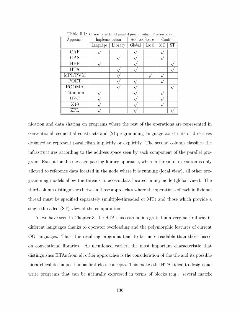
Table 5.1: Characterization of parallel programming infrastructures.
Approach Implementation Address Space ControlLanguage Library Global Local MT ST
CAF√ √ √
GAS√ √ √
HPF√ √ √
HTA√ √ √
MPI/PVM√ √ √
POET√ √ √
POOMA√ √ √
Titanium√ √ √
UPC√ √ √
X10√ √ √
ZPL√ √ √
nication and data sharing on programs where the rest of the operations are represented in
conventional, sequential constructs and (2) programming language constructs or directives
designed to represent parallelism implicitly or explicitly. The second column classifies the
infrastructures according to the address space seen by each component of the parallel pro-
gram. Except for the message-passing library approach, where a thread of execution is only
allowed to reference data located in the node where it is running (local view), all other pro-
gramming models allow the threads to access data located in any node (global view). The
third column distinguishes between those approaches where the operations of each individual
thread must be specified separately (multiple-threaded or MT) and those which provide a
single-threaded (ST) view of the computation.
As we have seen in Chapter 3, the HTA class can be integrated in a very natural way in
different languages thanks to operator overloading and the polymorphic features of current
OO languages. Thus, the resulting programs tend to be more readable than those based
on conventional libraries. As mentioned earlier, the most important characteristic that
distinguishes HTAs from all other approaches is the consideration of the tile and its possible
hierarchical decomposition as first-class concepts. This makes the HTAs ideal to design and
write programs that can be naturally expressed in terms of blocks (e.g.. several matrix
136

multiplication algorithms -Cannon [18], Summa [31]-, solvers such as LU, etc.) or which
can be solved recursively (e.g., FT). Such blocks can be used to achieve parallelism or data
locality or both, possibly using several levels of tiling for different purposes. With HTAs
it is easy to adjust the point where recursive computations end and the iterative solutions
start by changing the number of levels of tiling.
As shown in Table 5.1, HTA and POOMA [45] are the only library-based approaches
that provide a global view of the data and follow a single threaded programming approach.
This combination helps programmers’ productivity in at least two ways. First, programmers
can use familiar sequential programming languages, and reuse sequential modules, perhaps
with small changes. Therefore, programmers can write parallel programs practically in the
same way they write sequential programs. Second, the single-threaded semantics of HTAs
eases the transition from sequential to parallel because programmers need not be concerned
with the program’s behavior on a per processor basis, deadlocks, race conditions, etc., since
parallelism and synchronization are implicit. The single-threaded property also improves
readability. Furthermore, in the case of HTA, flattening enables incremental migration of
sequential applications to parallel form. This was the approach we followed in our translation
of the NAS benchmarks from sequential MATLAB to the HTA-based parallel version.
A good indication of the benefit of the single-threaded form is obtained by comparing
the number of lines of code of the HTA with those of MPI programs. Although the number
of lines of code is not the best metric to measure ease of programming, it can give a rough
estimate of program complexity. The plot in Figure 4.29 shows the lines of code for HTA
and MPI codes. A discussion on the SLOC measurements is already provided in Section 4.4.
A downside of the single-threaded approach is that asynchronous overlap is not easy to
express explicitly. However, much of this overlap can be achieved automatically with the
appropriate implementation (see Section 3.5.4).
A valuable property of a programming approach is the ability to convey to the program-
mers the cost of the execution of their code. This is particularly true in the case of parallel
137

environments, where communication costs can easily dominate the execution time. HTAs
are faithful to this idea: the statements that require data communication are clearly identi-
fied in the code either because of the usage of different indexes in the tiles, or because of the
invocation of functions that involve data communication (transposition, circular shift, etc.).
HTAs have also drawbacks. For example, just as the other global-view approaches [25],
they only allow limited forms of task-parallelism. Moreover, HTAs are suitable only for
array based programs. Though every program can be re-coded using array operations [37],
converting a general scalar program to its array equivalent is a difficult task and not suited
for naive programmers.
The most popular parallel programming approach for distributed-memory systems is the
use of a message passing library such as MPI [34] or PVM [32]. In this approach, the
programmer has a local view of the data structures and must write programs that execute in
a SPMD fashion. The communication and computation statements can be interleaved in an
unstructured manner, potentially leading to programs that are difficult to understand and
maintain.
An improvement over this approach is the usage of libraries that, while requiring SPMD
programming, provide the user with a global view of the data structures. This is the case of
the Global Arrays library [42] or the POET framework [6]. However, the SPMD program-
ming style and the requirement of explicit synchronization complicates programming.
Other libraries like POOMA [45] integrate their classes in a host OO language, and
exploit operator overloading and polymorphism in order to provide a global view of the data
and a single-threaded view of the computation, as our HTA library. However, POOMA
differs in fundamental ways from our approach. For example, while POOMA’s arrays can
be distributed in tiles, the library provides no easy means to explicitly refer to those tiles.
Also, hierarchical decomposition is not natural to POOMA’s arrays, while it is a defining
property of HTAs.
Several infrastructures are based on new languages with constructs to control concurrency
138

and distribution. As we can see in Table 5.1, all the language-based approaches provide a
global view of the data, but they can be classified in two groups according to their view of
the control flow: The multiple-threaded languages, like Co-Array Fortran (CAF) [43], Ti-
tanium [51],UPC [19] or X10 [17]; and single threaded form like High Performance Fortran
HPF [36, 38] and ZPL [48]. All these approaches (except HPF) share a common draw-
back: they force programmers to rewrite their applications in parallel from scratch, an effort
that can be ameliorated by providing interfaces with codes and libraries written in other
languages.
The control model of many language-based infrastructures is explicitly parallel SPMD in
which programmers are responsible for managing data distribution and low-level synchro-
nization. An advantage of these languages is that they are much more suitable than the
single-threaded counterparts for expressing task parallelism.
Another common characteristic of these languages is that they provide a Partitioned
Global Address Space (PGAS), in which any thread of execution can create objects that can
be accessed by other threads. And each thread and piece of data is associated with exactly
one node of execution. They typically provide also constructs to distinguish between remote
and local accesses. This helps programmers reason about the cost of their codes.
In single-threaded languages, communication and synchronization are no longer the re-
sponsibility of the programmer, but of the compiler. Programs written in this model tend
to be shorter and easier to understand and maintain than those expressed in local view
languages, which increases programmers’ productivity. The downsides of these languages
are their limited ability to express irregular parallelism and the responsibility they put on
compiler technology, which may not be developed enough to generate efficient codes in some
situations.
Different strategies have been studied to provide parallel codes with a global view of the
algorithms to execute. For example, High Performance Fortran (HPF) [36, 38] annotates
sequential Fortran codes with directives that specify array distribution, loop scheduling, etc.
139

These directives are optional, and there is little information about how the compiler will
translate them. The lack of a clear performance model makes it difficult for programmers
to reason about an algorithm’s performance.[41].
Another approach is to design a language from scratch, which is the case of ZPL. This
language is designed in order to minimize the effort of the compiler. Its syntax allows to
identify the operations that generate communication and their qualitative cost in a similar
way to our HTAs. However, they suffer from several drawbacks, chief among them being the
cost of migrating the software to an entirely new language.
140

Chapter 6
Conclusions
6.1 Conclusions
High performance programs exploit the parallelism and the locality of reference inherent in
a computation. Development of high performance programs that are clear, readable and
at the same time efficient is very difficult. The major difficulty is due to the absence of
language constructs that allow programmers to express parallelism and locality easily. This
thesis introduced a data type - Hierarchically Tiled Arrays - that allows the programmer to
explicitly control parallelism and locality.
The thesis identified several issues related to HTA. The issues pertain to implementing
the HTA in a conventional language, design of HTA operations and writing programs using
HTAs. The experiments reported by the thesis helped in identifying the performance bot-
tlenecks in HTA programs. Using these experiments, we have accurately characterized the
performance of HTA programs.
The key contributions of the thesis can be summarized as follows:
• Generalization of arrays - Hierarchically Tiled Arrays are generalizations of normal
arrays. The elements of the HTAs can be scalars or HTAs themselves. We formalized
several types of HTAs and several parameters associated with them.
• Generalization of array operations - We have extended several vector and array oper-
ations to HTAs. These operations are recursive and are straight forward extensions of
the existing array and vector operations. We also provide several higher order opera-
tions. A formal description of several HTA operations were provided. The semantics
141

of the operations are designed to eliminate potential ambiguities in interpreting them.
They also provide a consistent definition for both the programmers and potential HTA
compilers.
• Fusion with conventional languages - We have implemented the HTA in two popular
languages - C++ and MATLAB. This experiment revealed the issues in augmenting
sequential languages with the HTA data type. Essentially, we attempted to introduce
tiles as first class language constructs in conventional programming languages.
• Evaluation of HTA programs - We have written the programs from the NAS benchmark
set using the HTA data type. We started with a base sequential version of the pro-
grams and applied simple transformations to obtain the parallel HTA programs. This
experiment provided insight in to two key aspects of HTA programs - the impact on
programmer productivity and the impact on the program’s performance. We evaluated
the latter by executing the HTA programs on a cluster of up to 128 processors.
6.2 Future Work
6.2.1 Implementation of new language constructs
The thesis has identified new language constructs that will help improve both the syn-
tax of HTA programs and its performance. The two language constructs under study are
overlapped tiling and replicated HTA. In the programs like MG, LU, which involve stencil
computation, ghost regions are added to HTAs and programmer keeps them updated using
HTA assignment operation. Using overlapped tiling this can be done automatically. The
programmer only need to specify the depth of overlap among the tiles in each dimension,
while constructing the HTA. The shadow regions are added and kept updated internally by
the run time library.
Another useful language construct is replicated HTA. A replicated HTA of dimension
142

k is obtained by replicating a k-1 dimensional HTA along the dimension k. If the HTA
is sequential, such a replication is only logical. That is, only the structure is replicated,
but the data is shared among several tiles. If the HTA is distributed along the replicated
dimension, then an element is mapped to multiple processors. Updates to such an element
in one processor should be broadcast to other processors to which it is mapped. This kind
of HTA is useful to improve the clarity and performance of CG HTA program.
6.2.2 Improving the syntax of HTA programs
Another immediate future work is to improve the syntax of HTA programs, especially for
the CPP+HTA programs. This involves extending the grammar of the underlying language
(C++ or MATLAB). Given that the language of HTA is very light, the extension will be
very simple. For C++, a simple preprocessor can convert the HTA programs written in the
augmented language to the standard C++ language.
A more ambitious approach is to translate the MATLAB+HTA programs to CPP+HTA
programs using a high-level MATLAB compiler. In the past, few researchers have shown
the effectiveness of translating MATLAB to FORTRA90 and just-in-time compilation of
MATLAB [4] [46]. Since, MATLAB and HTA blend well without any syntax changes, using
it as the base language for HTA is a simpler and effective approach. Additionally, MATLAB
syntax is easier for a programmer than C++. A MATLAB+HTA to CPP+HTA translator
will benefit both productivity of the programmer and performance of the programs.
6.2.3 Improving the performance of HTA programs
We have shown that HTA programs are as efficient as MPI programs. We also have identified
several optimizations that are easily applicable to HTA programs, with minor changes to
source codes. These optimizations will further improve the performance of HTA programs.
For example, extending the split-phase semantics (cf Section 2.3.5) to other operations like
transpositions and permutations is one such valuable optimization, which is easy to express
143
using HTA operations. Yet another optimization is to implement HTA-aware algorithms for
reduction and scan operations. Such an algorithm will take in to account the tiling structure
of the HTA and schedule the communication and computation optimally.
144
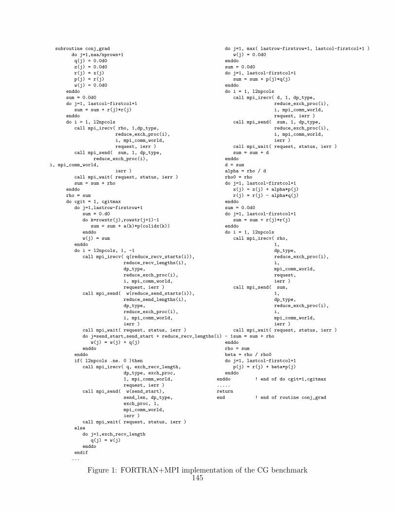
subroutine conj_grad
do j=1,naa/nprows+1
q(j) = 0.0d0
z(j) = 0.0d0
r(j) = x(j)
p(j) = r(j)
w(j) = 0.0d0
enddo
sum = 0.0d0
do j=1, lastcol-firstcol+1
sum = sum + r(j)*r(j)
enddo
do i = 1, l2npcols
call mpi_irecv( rho, 1,dp_type,
reduce_exch_proc(i),
i, mpi_comm_world,
request, ierr )
call mpi_send( sum, 1, dp_type,
reduce_exch_proc(i),
i, mpi_comm_world,
ierr )
call mpi_wait( request, status, ierr )
sum = sum + rho
enddo
rho = sum
do cgit = 1, cgitmax
do j=1,lastrow-firstrow+1
sum = 0.d0
do k=rowstr(j),rowstr(j+1)-1
sum = sum + a(k)*p(colidx(k))
enddo
w(j) = sum
enddo
do i = l2npcols, 1, -1
call mpi_irecv( q(reduce_recv_starts(i)),
reduce_recv_lengths(i),
dp_type,
reduce_exch_proc(i),
i, mpi_comm_world,
request, ierr )
call mpi_send( w(reduce_send_starts(i)),
reduce_send_lengths(i),
dp_type,
reduce_exch_proc(i),
i, mpi_comm_world,
ierr )
call mpi_wait( request, status, ierr )
do j=send_start,send_start + reduce_recv_lengths(i) - 1
w(j) = w(j) + q(j)
enddo
enddo
if( l2npcols .ne. 0 )then
call mpi_irecv( q, exch_recv_length,
dp_type, exch_proc,
1, mpi_comm_world,
request, ierr )
call mpi_send( w(send_start),
send_len, dp_type,
exch_proc, 1,
mpi_comm_world,
ierr )
call mpi_wait( request, status, ierr )
else
do j=1,exch_recv_length
q(j) = w(j)
enddo
endif
...
do j=1, max( lastrow-firstrow+1, lastcol-firstcol+1 )
w(j) = 0.0d0
enddo
sum = 0.0d0
do j=1, lastcol-firstcol+1
sum = sum + p(j)*q(j)
enddo
do i = 1, l2npcols
call mpi_irecv( d, 1, dp_type,
reduce_exch_proc(i),
i, mpi_comm_world,
request, ierr )
call mpi_send( sum, 1, dp_type,
reduce_exch_proc(i),
i, mpi_comm_world,
ierr )
call mpi_wait( request, status, ierr )
sum = sum + d
enddo
d = sum
alpha = rho / d
rho0 = rho
do j=1, lastcol-firstcol+1
z(j) = z(j) + alpha*p(j)
r(j) = r(j) - alpha*q(j)
enddo
sum = 0.0d0
do j=1, lastcol-firstcol+1
sum = sum + r(j)*r(j)
enddo
do i = 1, l2npcols
call mpi_irecv( rho,
1,
dp_type,
reduce_exch_proc(i),
i,
mpi_comm_world,
request,
ierr )
call mpi_send( sum,
1,
dp_type,
reduce_exch_proc(i),
i,
mpi_comm_world,
ierr )
call mpi_wait( request, status, ierr )
sum = sum + rho
enddo
rho = sum
beta = rho / rho0
do j=1, lastcol-firstcol+1
p(j) = r(j) + beta*p(j)
enddo
enddo ! end of do cgit=1,cgitmax
.....
return
end ! end of routine conj_grad
Figure 1: FORTRAN+MPI implementation of the CG benchmark145

subroutine transpose_x_yz(l1, l2, xin, xout)
call transpose2_local(dims(1,l1),
dims(2, l1)*dims(3, l1),
xin, xout)
call transpose2_global(xout, xin)
call transpose2_finish(dims(1,l1),
dims(2, l1)*dims(3, l1),
xin, xout)
return
end
subroutine transpose_xy_z(l1, l2, xin, xout)
call transpose2_local(dims(1,l1)*dims(2, l1),dims(3, l1),
xin, xout)
call transpose2_global(xout, xin)
call transpose2_finish(dims(1,l1)*dims(2, l1),dims(3, l1),
xin, xout)
return
end
subroutine transpose2_local(n1, n2, xin, xout)
do j = 1, n2
do i = 1, n1
xout(j, i) = xin(i, j)
end do
end do
return
end
subroutine transpose2_global(xin, xout)
call mpi_alltoall(xin, ntdivnp/np, dc_type,
xout, ntdivnp/np, dc_type,
commslice1, ierr)
end
subroutine transpose2_finish(n1, n2, xin, xout)
do p = 0, np2-1
ioff = p*n2
do j = 1, n1/np2
do i = 1, n2
xout(i+ioff, j) = xin(i, j, p)
end do
end do
end do
end
Figure 2: Transpositions in FT benchmark in FORTRAN+MPI version : x yz and xy ztranspositioon
146

subroutine transpose_x_z(l1, l2, xin, xout)
call transpose_x_z_local(dims(1,l1),xin, xout)
call transpose_x_z_global(dims(1,l1), xout, xin)
call transpose_x_z_finish(dims(1,l2), xin, xout)
return
end
subroutine transpose_x_z_local(d, xin, xout)
do j = 1, d(2)
do k = 1, d(3)
do i = 1, d(1)
xout(k, j, i) = xin(i, j, k)
end do
end do
end do
end
subroutine transpose_x_z_global(d, xin, xout)
call mpi_alltoall(xin, d(1)*d(2)*d(3)/np2, dc_type,
xout, d(1)*d(2)*d(3)/np2, dc_type,
commslice1, ierr)
do p = 0, np2-1
ioff = p*d(1)/np2
do k = 1, d(3)
do j = 1, d(2)
do i = 1, d(1)/np2
xout(i+ioff, j, k) = xin(i, j, k, p)
end do
end do
end do
end do
return
end
subroutine transpose_x_y(l1, l2, xin, xout)
call transpose_x_y_local(dims(1,l1),xin, xout)
call transpose_x_y_global(dims(1,l1), xout, xin)
call transpose_x_y_finish(dims(1,l1), xin, xout)
return
end
subroutine transpose_x_y_local(d, xin, xout)
do k = 1, d(3)
do i = 1, d(1)
do j = 1, d(2)
xout(j,k,i)=xin(i,j,k)
end do
end do
end do
return
end
subroutine transpose_x_y_global(d, xin, xout)
call mpi_alltoall(xin, d(1)*d(2)*d(3)/np1, dc_type,
xout, d(1)*d(2)*d(3)/np1, dc_type,
commslice2, ierr)
end
subroutine transpose_x_y_finish(d, xin, xout)
do p = 0, np1-1
ioff = p*d(1)/np1
do k = 1, d(3)
do j = 1, d(2)
do i = 1, d(1)/np1
xout(i+ioff, j, k) = xin(i, k, j, p)
end do
end do
end do
end do
return
end
(c)
Figure 3: Transpositions in FT benchmark in FORTRAN+MPI version (a) x z transposition(b) x y transposition
147
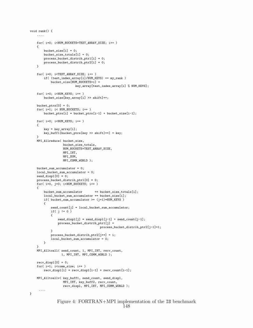
void rank() {
....
for( i=0; i<NUM_BUCKETS+TEST_ARRAY_SIZE; i++ )
{
bucket_size[i] = 0;
bucket_size_totals[i] = 0;
process_bucket_distrib_ptr1[i] = 0;
process_bucket_distrib_ptr2[i] = 0;
}
for( i=0; i<TEST_ARRAY_SIZE; i++ )
if( (test_index_array[i]/NUM_KEYS) == my_rank )
bucket_size[NUM_BUCKETS+i] =
key_array[test_index_array[i] % NUM_KEYS];
for( i=0; i<NUM_KEYS; i++ )
bucket_size[key_array[i] >> shift]++;
bucket_ptrs[0] = 0;
for( i=1; i< NUM_BUCKETS; i++ )
bucket_ptrs[i] = bucket_ptrs[i-1] + bucket_size[i-1];
for( i=0; i<NUM_KEYS; i++ )
{
key = key_array[i];
key_buff1[bucket_ptrs[key >> shift]++] = key;
}
MPI_Allreduce( bucket_size,
bucket_size_totals,
NUM_BUCKETS+TEST_ARRAY_SIZE,
MPI_INT,
MPI_SUM,
MPI_COMM_WORLD );
bucket_sum_accumulator = 0;
local_bucket_sum_accumulator = 0;
send_displ[0] = 0;
process_bucket_distrib_ptr1[0] = 0;
for( i=0, j=0; i<NUM_BUCKETS; i++ )
{
bucket_sum_accumulator += bucket_size_totals[i];
local_bucket_sum_accumulator += bucket_size[i];
if( bucket_sum_accumulator >= (j+1)*NUM_KEYS )
{
send_count[j] = local_bucket_sum_accumulator;
if( j != 0 )
{
send_displ[j] = send_displ[j-1] + send_count[j-1];
process_bucket_distrib_ptr1[j] =
process_bucket_distrib_ptr2[j-1]+1;
}
process_bucket_distrib_ptr2[j++] = i;
local_bucket_sum_accumulator = 0;
}
}
MPI_Alltoall( send_count, 1, MPI_INT, recv_count,
1, MPI_INT, MPI_COMM_WORLD );
recv_displ[0] = 0;
for( i=1; i<comm_size; i++ )
recv_displ[i] = recv_displ[i-1] + recv_count[i-1];
MPI_Alltoallv( key_buff1, send_count, send_displ,
MPI_INT, key_buff2, recv_count,
recv_displ, MPI_INT, MPI_COMM_WORLD );
....
}
Figure 4: FORTRAN+MPI implementation of the IS benchmark148

References
[1] High Performance Fortran Forum. High Performance Fortran Specification Version 2.0,January 1997.
[2] MATLAB: The Language of Technical Computing. 2006. http://www.mathworks.com.
[3] V. Adve and J. Mellor-Crummey. Using integer sets for data-parallel program analysisand optimization. In Proc. of the ACM SIGPLAN 1998 conf. on Programming languagedesign and implementation, pages 186–198. ACM Press, 1998.
[4] G. Almasi and D. A. Padua. MaJIC: A Matlab just-in-time compiler. Lecture Notes inComputer Science, 2017:68–81, 2001.
[5] G. Almasi, L. De Rose, B. B. Fraguela, J. Moreira, and D. Padua. Programming forLocality and Parallelism with Hierarchically Tiled Arrays. In Proc. of LCPC 2003,volume 2958 of LCNS, pages 162–176, College Station, Texas, Oct 2003. Springer-Verlag, New York.
[6] R. C. Armstrong and A. Cheung. POET (Parallel Object-oriented Environment andToolkit) and Frameworks for Scientific Distributed Computing. In Proc. of 30th HawaiiInternational Conference on System Sciences (HICSS 1997), pages 54–63, Maui, Hawai,1997.
[7] D. Bailey, E. Barszcz, J. Barton, D. Browning, R. Carterand L. Dagum, R. Fatoohi,S. Fineberg, P. Frederickson, T. Lasinski, R. Schreiber, H. Simon, V. Venkatakrishnan,and S. Weeratunga. The NAS Parallel Benchmarks. Technical Report RNR-94-007,RNR Technical Report, March 1994.
[8] G. H. Barnes, R. M. Brown, M. Kato, D.J. Kuck, D.L. Slotnick, and R.A. Stokes. TheILLIAC IV Computer. IEEE Trans., 8(17):746–757, 1968.
[9] E. Barszcz, R. Fatoohi, V. Venkatakrishnan, and S. Weeratunga. Solution of Regular,Sparse Triangular Linear Systems on Vector and Distributed-Memory Multiprocessors. Technical Report RNR-93-007, RNR Technical Report, April 1993.
[10] C. Barton, C. Cascaval, S. Chatterjee, G. Almasi, Y. Zheng, M. Farreras, and J. Ama-ral. Shared memory programming for large scale machines. In Proc. of the Conf. onProgramming Language Design and Implementation (PLDI), pages 108–117, 2006.
149
[11] G. Bikshandi, J. Guo, D. Hoeflinger, G. Almasi, B. B. Fraguela, Maria J. Garzaran, andD. Padua. Implementation of parallel numerical algorithms using hierarchically tiledarrays.
[12] G. Bikshandi, J. Guo, D. Hoeflinger, G. Almasi, B. B. Fraguela, Maria J. Garzaran,D. Padua, and Christoph von Praun. Programming for parallelism and locality withhierarchically tiled arrays. In PPoPP ’06: Proceedings of the eleventh ACM SIGPLANsymposium on Principles and practice of parallel programming, pages 48–57, New York,NY, USA, 2006. ACM Press.
[13] G. Bikshandi, C. Praun J. Guo, G. Tanase, B. B. Fraguela, M. J. Garzaran, D. Padua,and L. Rauchwerger. Design and Use of htalib – a Library for Hierarchically TiledArrays. In Procs. of the Languages and Compilers for Parallel Computing, 2006.
[14] G. E. Blelloch and G. W. Sabot. Compiling collection-oriented languages onto massivelyparallel computers. Journal of Parallel and Distributed Computing, 8(2):119–134, 1990.
[15] W. S. Brainerd, C. Goldberg, and J. Adams. Programmer’s guide to Fortran 90. Inter-text Publications, Inc.,/McGraw-Hill, Inc., New York, NY, USA, 1990.
[16] J. A. Brown and H. P. Crowder. APL2: Getting started. IBM Systems Journal,30(4):433–444, 1991.
[17] P. C., Ch. Donawa, K. Ebcioglu, Ch. Grothoff, A. Kielstra, Ch. von Praun, V. Saraswat,and V. Sarkar. X10: An Object-oriented Approach to Non-uniform Cluster Comput-ing. In Procs. of the Conf. on Object-Oriented Programming, Systems, Languages, andApplications (OOPSLA) – Onward! Track, Oct 2005.
[18] L.E. Cannon. A Cellular Computer to Implement the Kalman Filter Algorithm. PhDthesis, Montana State University, 1969.
[19] W. Carlson, J. Draper, D. Culler, K. Yelick, E. Brooks, and K. Warren. Introduction toUPC and Language Specification. Technical Report CCS-TR-99-157, IDA Center forComputing Sciences, 1999.
[20] S. Chakrabarti, B. E. Dom, S. Ravi Kumar, P. Raghavan, S. Rajagopalan, A. Tomkins,D. Gibson, and Jon Kleinberg. Mining the Web’s link structure. Computer, 32(8):60–67,1999.
[21] B.L. Chamberlain, S.Choi, E.C. Lewis, C. Lin, L. Synder, and W.D. Weathersby. TheCase for High Level Parallel Programming in ZPL. IEEE Computational Science andEngineering, 5(3):76–86, July–September 1998.
[22] B.M. Chapman, P. Mehrotra, and H. P. Zima. Vienna Fortrana Fortran LanguageExtension for Distributed Memory Multiprocessors. Languages, Compilers and Run-time Environments for Distributed Memory Machines, pages 39–62, 1992.
150

[23] D. E. Culler, A. Dusseau, S. Copen Goldstein, A. Krishnamurthy, S. Lumetta, Thorstenvon Eicken, and Katherine Yelick. Parallel programming in split-c. In Conference onSupercomputing (SC), pages 262–273, 1993.
[24] J. Dean and S. Ghemawat. Mapreduce: Simplified data processing on large clusters. InSymposium on Operating System Design and Implementation (OSDI), 2004.
[25] S. J. Deitz. Renewed Hope for Data Parallelism: Unintegrated Support for Task Par-allelism in ZPL. Technical Report UW-CSE-03-12-04, University of Washington, Dec2003.
[26] M. A. Ellis and B. Stroustrup. The annotated C++ reference manual. Addison-WesleyLongman Publishing Co., Inc., Boston, MA, USA, 1990.
[27] B. Chamberlain et al. ZPL’s WYSIWYG Performance Model. In Procs. of the High-Level Parallel Programming Models and Supportive Environments, pages 50–61. IEEEComputer Society, 1998.
[28] K. Fatahalian, T. J. Knight, M. Houston, M. Erez, D. Reiter Horn, L. Leem, J. Y. Park,M. Ren, A. Aiken, W. J. Dally, and Pat Hanrahan. Sequoia: Programming the memoryhierarchy. In Proceedings of the 2006 ACM/IEEE Conference on Supercomputing, 2006.
[29] M. Frigo. A fast Fourier transform compiler. In Proc. 1999 ACM SIGPLAN Conf. onProgramming Language Design and Implementation, volume 34, pages 169–180. ACM,May 1999.
[30] M. Frigo and S. G. Johnson. The design and implementation of FFTW3. Proceedingsof the IEEE, 93(2):216–231, 2005. special issue on ”Program Generation, Optimization,and Platform Adaptation”.
[31] R. A. Van De Geijn and J. Watts. SUMMA: Scalable Universal Matrix MultiplicationAlgorithm. Concurrency: Practice and Experience, 9(4):255–274, Apr 1997.
[32] A. Geist, A. Beguelin, J. Dongarra, W. J.ng, R. Manchek, and V. S. Sunderamet.PVM: Parallel Virtual Machine: A Users’ Guide and Tutorial for Networked ParallelComputing. MIT Press, 1994.
[33] S. L. Graham, P. B. Kessler, and M. K. Mckusick. Gprof: A call graph executionprofiler. SIGPLAN Not., 17(6):120–126, 1982.
[34] W. Gropp, E. Lusk, and A. Skjellum. Using MPI (2nd ed.): Portable Parallel Program-ming with the Message-Passing Interface”. MIT Press, 1999.
[35] J. Guo. Using HTAs for Locality (Ph.D. proposal). Technical report, University ofIllinois at Urbana-Champaign, June 2006.
[36] S. Hiranandani, K. Kennedy, and C.-W. Tseng. Compiling Fortran D for MIMDDistributed-memory Machines. Commun. ACM, 35(8):66–80, 1992.
151
[37] K. E. Iverson. A Programming Language. John Wiley & Sons, 1962.
[38] C. Koelbel and P. Mehrotra. An Overview of High Performance Fortran. SIGPLANFortran Forum, 11(4):9–16, 1992.
[39] J. Merlin and A. Hey. An introduction to high performance fortran. Sci. Program.,4(2):87–113, 1995.
[40] T. Ngo, L. Snyder, and B. Chamberlain. Portable performance of data parallel lan-guages. In Supercomputing ’97: Proceedings of the 1997 ACM/IEEE conference onSupercomputing (CDROM), pages 1–20, New York, NY, USA, 1997. ACM Press.
[41] T. A. Ngo. The Role of Performance Models in Parallel Programming and Languages.PhD thesis, Department of Computer Science and Engineering, University of Washing-ton, 1997.
[42] J. Nieplocha, R. J. Harrison, and R. J. Littlefield. Global arrays: a portable shared-memory programming model for distributed memory computers. In Supercomputing’94: Proc. of the 1994 Conf. on Supercomputing, pages 340–ff., Los Alamitos, CA,USA, 1994. IEEE Computer Society Press.
[43] R. W. Numrich and J. Reid. Co-array Fortran for Parallel Programming. SIGPLANFortran Forum, 17(2):1–31, 1998.
[44] D. Pham and et al. The Design and Implementation of a First-generation Cell Processor.In Procs. of the IEEE Solid-State Circuits Symposium, February 2005.
[45] J. V. W. Reynders, P. J. Hinker, J. C. Cummings, S. R. Atlas, S. Banerjee, W. F.Humphrey, S. R. Karmesin, K. Keahey, M. Srikant, and M. D. Tholburn. POOMA: AFramework for Scientific Simulations of Paralllel Architectures. In Gregory V. Wilsonand Paul Lu, editors, Parallel Programming in C++, pages 547–588. MIT Press, 1996.
[46] L. De Rose and D. A. Padua. A MATLAB to fortran 90 translator and its effectiveness.In International Conference on Supercomputing, pages 309–316, 1996.
[47] Jay M. Sipelstein and Guy E. Blelloch. Collection-Oriented Languages. Proceedings ofthe IEEE, 79(4):504–523, April 1991.
[48] L. Snyder. ZPL Programming Guide. 1999.
[49] T. Veldhuizen. Techniques for Scientific C++, August 1999.
[50] M. E. Wolf and M. S. Lam. A Data Locality Optimizing Algorithm. In PLDI, pages30–44. ACM Press, 1991.
[51] K. A. Yelick, L. Semenzato, G. Pike, C. Miyamoto, B. Liblit, A. Krishnamurthy,P. N. Hilfinger, S. L. Graham, D. Gay, P. Colella, and A. Aiken. Titanium: A High-Performance Java Dialect. In Workshop on Java for High-Performance Network Com-puting, February 1998.
152

Author’s Biography
Ganesh Bikshandi finished his PhD in computer science at the University of Illinois, Urbana-
Champaign. Earlier, he obtained his bachelor’s degree in computer science and engineering
from the University of Madras, India. He has worked for Intel and IBM research (T. J.
Watson) as summer intern. Upon graduation, he will be joining the IBM India research
labs.
153