calculus of variations and applications to solid mechanics€¦ · calculus of variations and...
TRANSCRIPT

Calculus of Variations and applications toSolid Mechanics
Carlos Mora-Corral
January 25–29 2010Overview
C. Mora-Corral Calculus of Variations and Solid Mechanics

Outline of the course
1 Introduction to Solid Mechanics. The equations ofElasticity.
2 Hyperelasticity. Polyconvexity. Existence of minimizers.3 Constitutive equations. Isotropic materials.4 Quasiconvexity and lower semicontinuity.5 Phase transitions in crystal solids. The shape memory
effect.
C. Mora-Corral Calculus of Variations and Solid Mechanics
IntroductionDescription of motion
The balance laws of continuum mechanicsNonlinear elasticity
Calculus of Variations and applications toSolid Mechanics
Carlos Mora-Corral
January 25–29 2010Lecture 1
C. Mora-Corral Calculus of Variations and Solid Mechanics
IntroductionDescription of motion
The balance laws of continuum mechanicsNonlinear elasticity
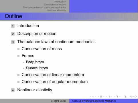
Outline
1 Introduction
2 Description of motion
3 The balance laws of continuum mechanics
Conservation of mass
ForcesBody forces
Surface forces
Conservation of linear momentum
Conservation of angular momentum
4 Nonlinear elasticity
C. Mora-Corral Calculus of Variations and Solid Mechanics
IntroductionDescription of motion
The balance laws of continuum mechanicsNonlinear elasticity
Outline
1 Introduction
2 Description of motion
3 The balance laws of continuum mechanics
Conservation of mass
ForcesBody forces
Surface forces
Conservation of linear momentum
Conservation of angular momentum
4 Nonlinear elasticity
C. Mora-Corral Calculus of Variations and Solid Mechanics

IntroductionDescription of motion
The balance laws of continuum mechanicsNonlinear elasticity
Rubber, steel, wood, rock, metals. . . can all be modelled byelasticity theory, even though their chemical structures andmaximum reversible strains are very different.
Elasticity theory in the central model of Solid Mechanics. Inthis course we will deal with nonlinear theory, which is validfor any deformation, whether large or small. There is also thelinear theory, which consists of a linearization of the model ofthe nonlinear theory, and is valid only for small deformations.
C. Mora-Corral Calculus of Variations and Solid Mechanics
IntroductionDescription of motion
The balance laws of continuum mechanicsNonlinear elasticity
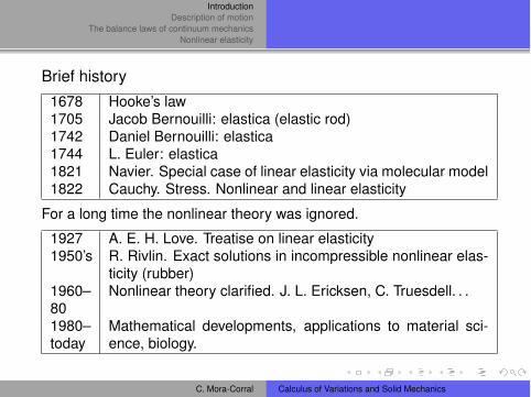
Brief history1678 Hooke’s law1705 Jacob Bernouilli: elastica (elastic rod)1742 Daniel Bernouilli: elastica1744 L. Euler: elastica1821 Navier. Special case of linear elasticity via molecular model1822 Cauchy. Stress. Nonlinear and linear elasticity
For a long time the nonlinear theory was ignored.
1927 A. E. H. Love. Treatise on linear elasticity1950’s R. Rivlin. Exact solutions in incompressible nonlinear elas-
ticity (rubber)1960–80
Nonlinear theory clarified. J. L. Ericksen, C. Truesdell. . .
1980–today
Mathematical developments, applications to material sci-ence, biology.
C. Mora-Corral Calculus of Variations and Solid Mechanics

IntroductionDescription of motion
The balance laws of continuum mechanicsNonlinear elasticity
Outline
1 Introduction
2 Description of motion
3 The balance laws of continuum mechanics
Conservation of mass
ForcesBody forces
Surface forces
Conservation of linear momentum
Conservation of angular momentum
4 Nonlinear elasticity
C. Mora-Corral Calculus of Variations and Solid Mechanics
IntroductionDescription of motion
The balance laws of continuum mechanicsNonlinear elasticity
For fluids, we commonly use the Eulerian or spatial descriptionof motion, fixing attention on a point ! in space, and studyinghow the velocity of the fluid v(!, t) varies with time t and spatialpoint !. Different particles of the fluid pass through ! at differenttimes. The Eulerian description is used mainly because in it thegoverning equations take a relatively simple form. However, thedescription is awkward when there are free boundaries, since apoint ! may be occupied by a fluid at some times, but not atothers.
C. Mora-Corral Calculus of Variations and Solid Mechanics
IntroductionDescription of motion
The balance laws of continuum mechanicsNonlinear elasticity
For solids, it is more convenient to use the Lagrangian ormaterial description of motion, in which we fix attention on agiven particle (or material point) and study how it moves. In thisdescription, free boundaries are described automatically.
We label the material points by the positions x = (x1, x2, x3)they occupy in a reference configuration, in which the solidoccupies a region ! ! R3. We assume that ! is open andconnected with a sufficiently smooth boundary "!.
C. Mora-Corral Calculus of Variations and Solid Mechanics

IntroductionDescription of motion
The balance laws of continuum mechanicsNonlinear elasticity
Let u(x, t) " R3 be the position occupied by the material pointx " ! at time t. Thus, u : !# (t1, t2)$ R3, for%& ' t1 < t2 ' &. In this first lecture, we suppose that u issufficiently smooth. Later, we will only assume that u isSobolev.
The deformation gradient is the differential of u with respect tox, denoted F = Du. In components,
Fi,! = ui,! ="ui
"x!, i,# = 1, 2, 3.
Notation: Greek indices for coordinates x!; Latin indices forcoordinates ui. Also, Einstein summation convention.
C. Mora-Corral Calculus of Variations and Solid Mechanics
IntroductionDescription of motion
The balance laws of continuum mechanicsNonlinear elasticity
To avoid interpenetration of matter, we require that for eachtime t, u(·, t) is invertible on !. We also suppose that u(·, t) isorientation-preserving:
J := detF (x, t) > 0 for x " !, t " (t1, t2).
C. Mora-Corral Calculus of Variations and Solid Mechanics
IntroductionDescription of motion
The balance laws of continuum mechanicsNonlinear elasticity
Conservation of massForcesConservation of linear momentumConservation of angular momentum
Outline
1 Introduction
2 Description of motion
3 The balance laws of continuum mechanics
Conservation of mass
ForcesBody forces
Surface forces
Conservation of linear momentum
Conservation of angular momentum
4 Nonlinear elasticity
C. Mora-Corral Calculus of Variations and Solid Mechanics
IntroductionDescription of motion
The balance laws of continuum mechanicsNonlinear elasticity
Conservation of massForcesConservation of linear momentumConservation of angular momentum
In what follows, E denotes an arbitrary open subset of ! withsufficiently smooth boundary "E. In a given motion u, thematerial points of E occupy the open region Et := u(E, t).
C. Mora-Corral Calculus of Variations and Solid Mechanics

IntroductionDescription of motion
The balance laws of continuum mechanicsNonlinear elasticity
Conservation of massForcesConservation of linear momentumConservation of angular momentum
Conservation of mass
Denote by $(y, t) the density of the body at y " !t at time t.The mass inside the region P ! !t at time t is
m(P, t) =!
P$(y, t) dy.
The density of the body in the reference configuration at thepoint x is denoted $R(x). The mass of the material occupyingE ! ! is
m(E) =!
E$R(x) dx.
C. Mora-Corral Calculus of Variations and Solid Mechanics
IntroductionDescription of motion
The balance laws of continuum mechanicsNonlinear elasticity
Conservation of massForcesConservation of linear momentumConservation of angular momentum
We assume the mass is conserved, i.e., for all E,
m(Et, t) = m(E).
Equivalently !
Et
$(y, t) dy =!
E$R(x) dx,
that is, !
E$(x, t) detDu(x, t) dx =
!
E$R(x) dx.
Hence !
E($J % $R) dx = 0 for all E,
i.e.,$J = $R.
C. Mora-Corral Calculus of Variations and Solid Mechanics
IntroductionDescription of motion
The balance laws of continuum mechanicsNonlinear elasticity
Conservation of massForcesConservation of linear momentumConservation of angular momentum
ForcesBody Forces
Let b(y, t) " R3 be the force exerted per unit mass by theexternal world. Thus, if E ! ! then
!
Et
$b dy =!
E$Rb dx
is the total body force exerted on Et at time t.
Example: Gravity takes the form
b(y, t) = %ge3.
C. Mora-Corral Calculus of Variations and Solid Mechanics

IntroductionDescription of motion
The balance laws of continuum mechanicsNonlinear elasticity
Conservation of massForcesConservation of linear momentumConservation of angular momentum
Surface forces
Cauchy’s hypothesis: There is a vector field s(y, t, n) " R3
(the Cauchy stress vector) with the following property:
Let S be a smooth oriented surface in !t with positive unitnormal n at y. Then s(y, t, n) is the force per unit area exertedacross S on the material on the negative side of S by thematerial on the positive side.
Thus, the resultant surface force on Et is given by!
"Et
s(y, t, n) da.
n = unit outward normal to "Et at y.da = surface area element = dH2(y).
C. Mora-Corral Calculus of Variations and Solid Mechanics
IntroductionDescription of motion
The balance laws of continuum mechanicsNonlinear elasticity
Conservation of massForcesConservation of linear momentumConservation of angular momentum
The Piola–Kirchhoff stress vector sR(x, t,N) is parallel to theCauchy stress vector s, but measures the surface force per unitarea in the reference configuration, acting across the(deformed) surface having normal N in the referenceconfiguration.
What is the relationship between deformed and undeformedareas, i.e., between da and dA?
C. Mora-Corral Calculus of Variations and Solid Mechanics
IntroductionDescription of motion
The balance laws of continuum mechanicsNonlinear elasticity
Conservation of massForcesConservation of linear momentumConservation of angular momentum
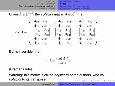
Given A " R3!3, the cofactor matrix A " R3!3 is
cof A =
"
######$
%%%%A22 A23
A32 A33
%%%% %%%%%A21 A23
A31 A33
%%%%
%%%%A21 A22
A31 A32
%%%%
%%%%%A12 A13
A32 A33
%%%%
%%%%A11 A13
A31 A33
%%%% %%%%%A11 A12
A31 A32
%%%%%%%%A12 A13
A22 A23
%%%% %%%%%A11 A13
A21 A23
%%%%
%%%%A11 A12
A21 A22
%%%%
&
''''''(.
If A is invertible, then
A"1 =(cof A)T
det A.
(Cramer’s rule).
Warning: this matrix is called adjoint by some authors, who callcofactor to its transpose.
C. Mora-Corral Calculus of Variations and Solid Mechanics
IntroductionDescription of motion
The balance laws of continuum mechanicsNonlinear elasticity
Conservation of massForcesConservation of linear momentumConservation of angular momentum
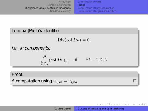
Lemma (Piola’s identity)
Div(cof Du) = 0,
i.e., in components,
"
"x!(cof Du)i! = 0 (i = 1, 2, 3.
Proof.A computation using ui,!# = ui,#!.
C. Mora-Corral Calculus of Variations and Solid Mechanics
IntroductionDescription of motion
The balance laws of continuum mechanicsNonlinear elasticity
Conservation of massForcesConservation of linear momentumConservation of angular momentum
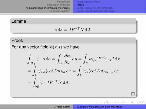
Lemma
n da = JF"T N dA.
Proof.For any vector field %(x, t) we have
!
"Et
% · n da =!
Et
"%i
"yidy =
!
E%i,!(F"1)!iJ dx
=!
E%i,!(cof Du)i! dx =
!
E[%i(cof Du)i!],! dx
=!
"E% · JF"T N dA.
C. Mora-Corral Calculus of Variations and Solid Mechanics
IntroductionDescription of motion
The balance laws of continuum mechanicsNonlinear elasticity
Conservation of massForcesConservation of linear momentumConservation of angular momentum
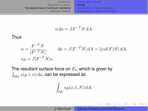
n da = JF"T N dA.
Thus
n =F"T N
|F"T N | , da = J |F"T N |dA = |(cof F )N |dA,
sR = J |F"T N |s.
The resultant surface force on Et, which is given by)"Et
s(y, t, n) da, can be expressed as!
"EsR(x, t,N) dA.
C. Mora-Corral Calculus of Variations and Solid Mechanics
IntroductionDescription of motion
The balance laws of continuum mechanicsNonlinear elasticity
Conservation of massForcesConservation of linear momentumConservation of angular momentum
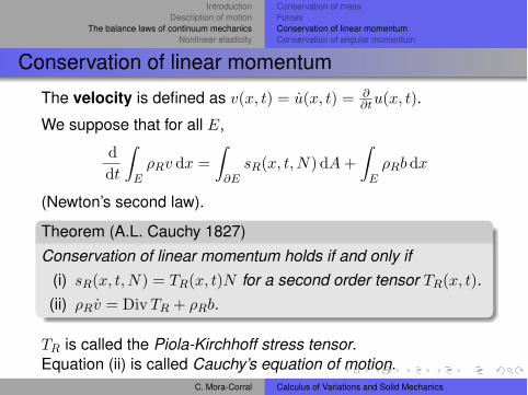
Conservation of linear momentum
The velocity is defined as v(x, t) = u(x, t) = ""tu(x, t).
We suppose that for all E,
ddt
!
E$Rv dx =
!
"EsR(x, t,N) dA +
!
E$Rb dx
(Newton’s second law).
Theorem (A.L. Cauchy 1827)Conservation of linear momentum holds if and only if
(i) sR(x, t,N) = TR(x, t)N for a second order tensor TR(x, t).(ii) $Rv = Div TR + $Rb.
TR is called the Piola-Kirchhoff stress tensor.Equation (ii) is called Cauchy’s equation of motion.
C. Mora-Corral Calculus of Variations and Solid Mechanics
IntroductionDescription of motion
The balance laws of continuum mechanicsNonlinear elasticity
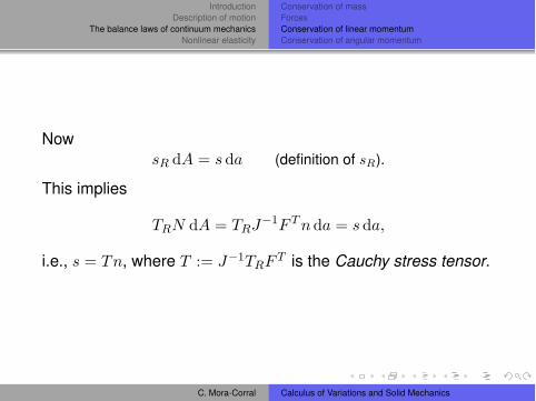
Conservation of massForcesConservation of linear momentumConservation of angular momentum
NowsR dA = sda (definition of sR).
This implies
TRN dA = TRJ"1F T n da = sda,
i.e., s = Tn, where T := J"1TRF T is the Cauchy stress tensor.
C. Mora-Corral Calculus of Variations and Solid Mechanics
IntroductionDescription of motion
The balance laws of continuum mechanicsNonlinear elasticity
Conservation of massForcesConservation of linear momentumConservation of angular momentum
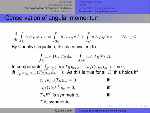
Conservation of angular momentum
ddt
!
Eu ) $Rv dx =
!
"Eu ) sR dA +
!
Eu ) $Rb dx (E ! !.
By Cauchy’s equation, this is equivalent to!
Eu )Div TR dx =
!
"Eu ) TRN dA.
In components,)E &ijk [uj(TR)k!,! % (ujTR k!),!] dx = 0,
iff)E &ijkuj,!(TR)k! dx = 0. As this is true for all E, this holds iff
&ijkuj,!(TR)k! = 0, iff
&ijk(TRF T )kj = 0, iff
TRF T is symmetric, iffT is symmetric.
C. Mora-Corral Calculus of Variations and Solid Mechanics
IntroductionDescription of motion
The balance laws of continuum mechanicsNonlinear elasticity
Outline
1 Introduction
2 Description of motion
3 The balance laws of continuum mechanics
Conservation of mass
ForcesBody forces
Surface forces
Conservation of linear momentum
Conservation of angular momentum
4 Nonlinear elasticity
C. Mora-Corral Calculus of Variations and Solid Mechanics
IntroductionDescription of motion
The balance laws of continuum mechanicsNonlinear elasticity
Up to now, our discussion applies to all materials (fluids,solids. . . ) for which Cauchy’s stress hypothesis applies. Tospecify the material, and make the equations determinate, weneed a constitutive equation, expressing the Piola–Kirchhoff (orCauchy) stress tensor in terms of the motion.
The need of a constitutive equation can also be seen from thefollowing heuristic argument. Up to now, we have Cauchy’sequation of motion
$Rv = Div TR + $Rb
and the fact that T is symmetric. Cauchy’s equation has
9 unknowns: 3 for v and 6 for TR.3 equations.
Therefore, 6 additional equations are necessary to solve theequations.
C. Mora-Corral Calculus of Variations and Solid Mechanics
IntroductionDescription of motion
The balance laws of continuum mechanicsNonlinear elasticity
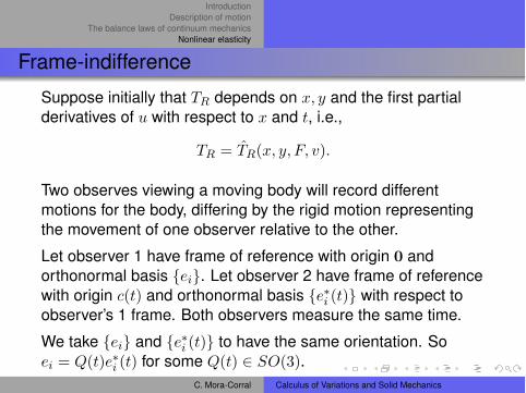
Frame-indifference
Suppose initially that TR depends on x, y and the first partialderivatives of u with respect to x and t, i.e.,
TR = TR(x, y, F, v).
Two observes viewing a moving body will record differentmotions for the body, differing by the rigid motion representingthe movement of one observer relative to the other.
Let observer 1 have frame of reference with origin 0 andorthonormal basis {ei}. Let observer 2 have frame of referencewith origin c(t) and orthonormal basis {e#i (t)} with respect toobserver’s 1 frame. Both observers measure the same time.
We take {ei} and {e#i (t)} to have the same orientation. Soei = Q(t)e#i (t) for some Q(t) " SO(3).
C. Mora-Corral Calculus of Variations and Solid Mechanics
IntroductionDescription of motion
The balance laws of continuum mechanicsNonlinear elasticity
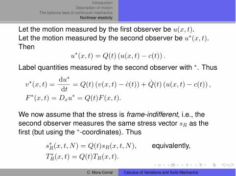
Let the motion measured by the first observer be u(x, t).Let the motion measured by the second observer be u#(x, t).Then
u#(x, t) = Q(t) (u(x, t)% c(t)) .
Label quantities measured by the second observer with #. Thus
v#(x, t) =du#
dt= Q(t) (v(x, t)% c(t)) + Q(t) (u(x, t)% c(t)) ,
F #(x, t) = Dxu# = Q(t)F (x, t).
We now assume that the stress is frame-indifferent, i.e., thesecond observer measures the same stress vector sR as thefirst (but using the #-coordinates). Thus
s#R(x, t,N) = Q(t)sR(x, t,N), equivalently,T #R(x, t) = Q(t)TR(x, t).
C. Mora-Corral Calculus of Variations and Solid Mechanics
IntroductionDescription of motion
The balance laws of continuum mechanicsNonlinear elasticity
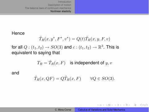
HenceTR(x, y#, F #, v#) = Q(t)TR(x, y, F, v)
for all Q : (t1, t2)$ SO(3) and c : (t1, t2)$ R3. This isequivalent to saying that
TR = TR(x, F ) is independent of y, v
andTR(x, QF ) = QTR(x, F ) (Q " SO(3).
C. Mora-Corral Calculus of Variations and Solid Mechanics

IntroductionDescription of motion
The balance laws of continuum mechanicsNonlinear elasticity
DefinitionA material is elastic if it has constitutive equation of the form
TR = TR(x, F ),
and hyperelastic if in addition
TR(x, F ) = DF W (x, F )
for some W : !# R3!3 $ R. In components,
(TR)i!(x, F ) ="W
"Fi!(x, F ) (x " !, F " R3!3, i,# " {1, 2, 3}.
C. Mora-Corral Calculus of Variations and Solid Mechanics
IntroductionDescription of motion
The balance laws of continuum mechanicsNonlinear elasticity
From now on, we consider only hyperelastic materials that arealso homogeneous, i.e., W is independent of x, so that
TR(F ) = DW (F ).
These materials have the same material response at everypoint.
W : R3!3 $ R is called the stored-energy function.
From thermodynamics, we get the interpretation that!
!W (Du(x, t)) dx
is the elastic energy stored by the body at time t.
C. Mora-Corral Calculus of Variations and Solid Mechanics
IntroductionDescription of motion
The balance laws of continuum mechanicsNonlinear elasticity
It is easy to see that
TR(QF ) = QTR(F ) iff W (QF ) = W (F )
(for all F " R3!3 and Q " SO(3)), and that, if this is the case,then
T is symmetric.
Hence, the conservation of angular momentum is automaticallysatisfied for hyperelastic materials.
C. Mora-Corral Calculus of Variations and Solid Mechanics
Calculus of Variations and applications toSolid Mechanics
Carlos Mora-Corral
January 25–29 2010Lecture 2
C. Mora-Corral Calculus of Variations and Solid Mechanics
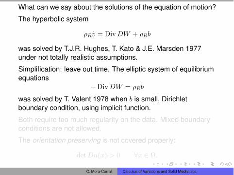
What can we say about the solutions of the equation of motion?
The hyperbolic system
!Rv = Div DW + !Rb
was solved by T.J.R. Hughes, T. Kato & J.E. Marsden 1977under not totally realistic assumptions.
Simplification: leave out time. The elliptic system of equilibriumequations
!Div DW = !Rb
was solved by T. Valent 1978 when b is small, Dirichletboundary condition, using implicit function.
Both require too much regularity on the data. Mixed boundaryconditions are not allowed.
The orientation preserving is not covered properly:
detDu(x) > 0 "x # !.
C. Mora-Corral Calculus of Variations and Solid Mechanics
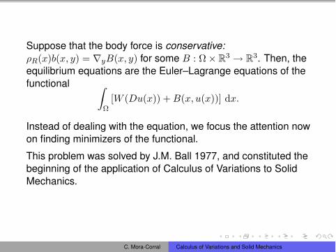
Suppose that the body force is conservative:!R(x)b(x, y) = $yB(x, y) for some B : !% R3 & R3. Then, theequilibrium equations are the Euler–Lagrange equations of thefunctional !
![W (Du(x)) + B(x, u(x))] dx.
Instead of dealing with the equation, we focus the attention nowon finding minimizers of the functional.
This problem was solved by J.M. Ball 1977, and constituted thebeginning of the application of Calculus of Variations to SolidMechanics.
C. Mora-Corral Calculus of Variations and Solid Mechanics

The direct method of the Calculus of Variations
PropositionLet X be a topological space. Let I : X & R ' {(} be
Coercive: for each M # R, the set {u # X : I[u] )M} issequentially compact.Sequentially lower semicontinuous: if lim
n!"un = u then
I[u] ) lim infn!"
I[un].
Then there exists a minimizer of I in X, i.e.,
*u0 # X such that I[u0] = infu#X
I[u].
Proof.Let un be a minimizing sequence. Then, for a subsequence,un & u0 # X, and I[u0] ) inf I.
C. Mora-Corral Calculus of Variations and Solid Mechanics
Compactness and (semi-)continuity are antagonistic in atopological space, in the sense that
The stronger the topology is (i.e., the more open sets thereare), the more continuous functions there are, and thefewer compact sets there are.The weaker the topology is (i.e., the fewer open sets thereare), the fewer continuous functions there are, and themore compact sets there are.
Our original problem is to find minimizers on a set. This setdoes not have a priori a topology. The use of a topology is atrick that we use in order to find minimizers.
The idea is to construct a topology that is not too weak and nottoo strong so that there are enough compact sets and enough(semi-)continuous functions.
C. Mora-Corral Calculus of Variations and Solid Mechanics
In Nonlinear elasticity, the central concept is the stress
TR = TR(x, Du(x)),
whereas in hyperelasticity, the central concept is the energy W ,from which the stress TR can be derived. The total energy of adeformation is !
!W (Du(x)) dx.
So the functional space where to look for minimizers shouldconsists of a space of functions with one derivative. C1 is not agood space because its topology is too strong (if we use thenorm topology) or too weak (if we use the pointwise topology).
If W (F ) + |F |p then the natural space is W 1,p(!, R3). In fact,the weak topology in W 1,p gives us a good compromisebetween compactness and (semi-)continuity.
C. Mora-Corral Calculus of Variations and Solid Mechanics
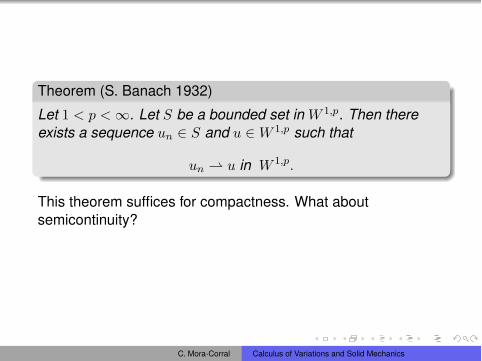
Theorem (S. Banach 1932)
Let 1 < p <(. Let S be a bounded set in W 1,p. Then thereexists a sequence un # S and u #W 1,p such that
un " u in W 1,p.
This theorem suffices for compactness. What aboutsemicontinuity?
C. Mora-Corral Calculus of Variations and Solid Mechanics

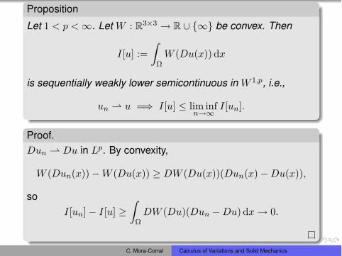
Proposition
Let 1 < p <(. Let W : R3$3 & R ' {(} be convex. Then
I[u] :=!
!W (Du(x)) dx
is sequentially weakly lower semicontinuous in W 1,p, i.e.,
un " u =, I[u] ) lim infn!"
I[un].
Proof.Dun " Du in Lp. By convexity,
W (Dun(x))!W (Du(x)) - DW (Du(x))(Dun(x)!Du(x)),
soI[un]! I[u] -
!
!DW (Du)(Dun !Du) dx& 0.
C. Mora-Corral Calculus of Variations and Solid Mechanics
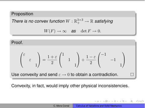
Proposition
There is no convex function W : R3$3+ & R satisfying
W (F )&( as det F & 0.
Proof.
"
##
#1
$
% =1 + #
2
"
#1
11
$
% +1! #
2
"
#!1
!11
$
%
Use convexity and send #& 0 to obtain a contradiction.
Convexity, in fact, would imply other physical inconsistencies.
C. Mora-Corral Calculus of Variations and Solid Mechanics
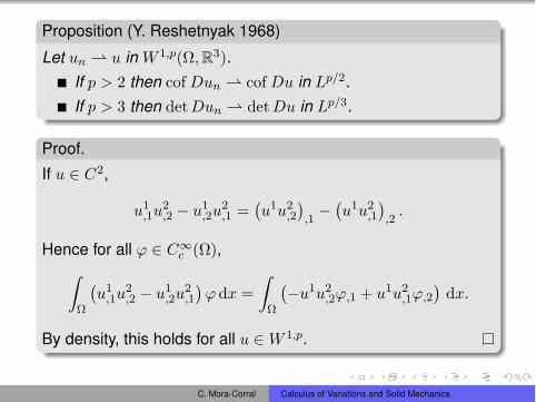
Proposition (Y. Reshetnyak 1968)
Let un " u in W 1,p(!, R3).If p > 2 then cof Dun " cof Du in Lp/2.If p > 3 then det Dun " det Du in Lp/3.
Proof.If u # C2,
u1,1u
2,2 ! u1
,2u2,1 =
&u1u2
,2
',1!
&u1u2
,1
',2
.
Hence for all $ # C"c (!),!
!
&u1
,1u2,2 ! u1
,2u2,1
'$ dx =
!
!
&!u1u2
,2$,1 + u1u2,1$,2
'dx.
By density, this holds for all u #W 1,p.
C. Mora-Corral Calculus of Variations and Solid Mechanics
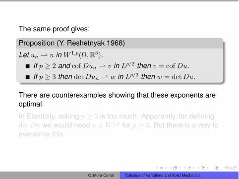
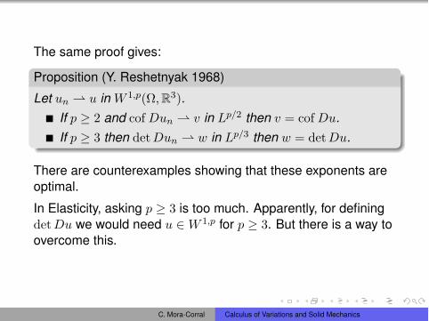
The same proof gives:
Proposition (Y. Reshetnyak 1968)
Let un " u in W 1,p(!, R3).If p - 2 and cof Dun " v in Lp/2 then v = cof Du.If p - 3 then det Dun " w in Lp/3 then w = detDu.
There are counterexamples showing that these exponents areoptimal.
In Elasticity, asking p - 3 is too much. Apparently, for definingdet Du we would need u #W 1,p for p - 3. But there is a way toovercome this.
C. Mora-Corral Calculus of Variations and Solid Mechanics
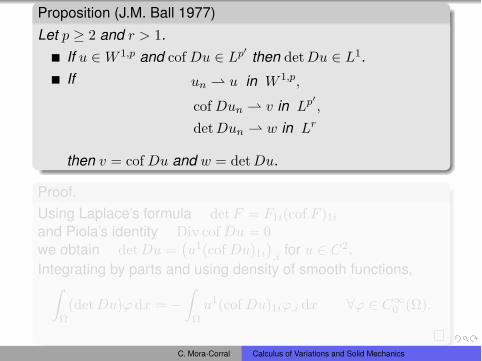
Proposition (J.M. Ball 1977)Let p - 2 and r > 1.
If u #W 1,p and cof Du # Lp! then det Du # L1.If un " u in W 1,p,
cof Dun " v in Lp!,
det Dun " w in Lr
then v = cof Du and w = detDu.
Proof.Using Laplace’s formula detF = F1i(cof F )1i
and Piola’s identity Div cof Du = 0we obtain det Du =
&u1(cof Du)1i
',i
for u # C2.Integrating by parts and using density of smooth functions,
!
!(detDu)$ dx = !
!
!u1(cof Du)1i$,i dx "$ # C"0 (!).
C. Mora-Corral Calculus of Variations and Solid Mechanics
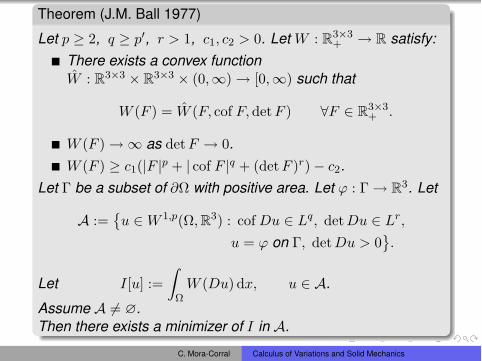
Theorem (J.M. Ball 1977)
Let p - 2, q - p%, r > 1, c1, c2 > 0. Let W : R3$3+ & R satisfy:
There exists a convex functionW : R3$3 % R3$3 % (0,()& [0,() such that
W (F ) = W (F, cof F,det F ) "F # R3$3+ .
W (F )&( as det F & 0.W (F ) - c1(|F |p + | cof F |q + (det F )r)! c2.
Let " be a subset of %! with positive area. Let $ : "& R3. Let
A :=(u #W 1,p(!, R3) : cof Du # Lq, detDu # Lr,
u = $ on ", det Du > 0).
Let I[u] :=!
!W (Du) dx, u # A.
Assume A .= !.Then there exists a minimizer of I in A.
C. Mora-Corral Calculus of Variations and Solid Mechanics
We can add forces to the total energy:!
!f · u dx +
!
!!\"g · u da.
C. Mora-Corral Calculus of Variations and Solid Mechanics
Analysis of strainMaterial symmetry
Incompressible elasticityConstitutive equations for rubber
Initial and boundary conditionsExamples of non-uniqueness of equilibrium solutions
Calculus of Variations and applications toSolid Mechanics
Carlos Mora-Corral
January 25–29 2010Lecture 3
C. Mora-Corral Calculus of Variations and Solid Mechanics
Analysis of strainMaterial symmetry
Incompressible elasticityConstitutive equations for rubber
Initial and boundary conditionsExamples of non-uniqueness of equilibrium solutions
Outline
1 Analysis of strain
2 Material symmetry
3 Incompressible elasticity
4 Constitutive equations for rubber
5 Initial and boundary conditions
6 Examples of non-uniqueness of equilibrium solutions
C. Mora-Corral Calculus of Variations and Solid Mechanics
Analysis of strainMaterial symmetry
Incompressible elasticityConstitutive equations for rubber
Initial and boundary conditionsExamples of non-uniqueness of equilibrium solutions
Preliminaries from linear algebraLocal state of strainInvariants
Analysis of strainPreliminaries from linear algebra
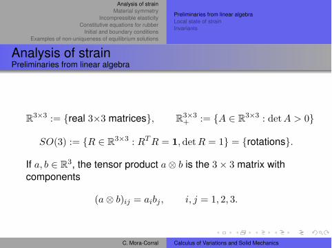
R3!3 := {real 3!3 matrices}, R3!3+ := {A " R3!3 : detA > 0}
SO(3) := {R " R3!3 : RT R = 1,det R = 1} = {rotations}.
If a, b " R3, the tensor product a# b is the 3! 3 matrix withcomponents
(a# b)ij = aibj , i, j = 1, 2, 3.
C. Mora-Corral Calculus of Variations and Solid Mechanics
Analysis of strainMaterial symmetry
Incompressible elasticityConstitutive equations for rubber
Initial and boundary conditionsExamples of non-uniqueness of equilibrium solutions
Preliminaries from linear algebraLocal state of strainInvariants
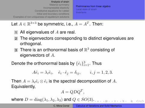
Let A " R3!3 be symmetric, i.e., A = AT . Then:
1 All eigenvalues of A are real.2 The eigenvectors corresponding to distinct eigenvalues are
orthogonal.3 There is an orthonormal basis of R3 consisting of
eigenvectors of A.
Denote the orthonormal basis by {ei}3i=1. Thus
Aei = !iei, ei · ej = "ij , i, j = 1, 2, 3.
Then A = !iei # ei is the spectral decompostition of A.Equivalently,
A = QDQT ,
where D = diag(!1, !2, !3) and Q " SO(3).C. Mora-Corral Calculus of Variations and Solid Mechanics
Analysis of strainMaterial symmetry
Incompressible elasticityConstitutive equations for rubber
Initial and boundary conditionsExamples of non-uniqueness of equilibrium solutions
Preliminaries from linear algebraLocal state of strainInvariants
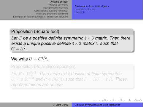
Proposition (Square root)Let C be a positive definite symmetric 3! 3 matrix. Then thereexists a unique positive definite 3! 3 matrix U such thatC = U2.
We write U = C1/2.
Proposition (Polar decomposition)
Let F " R3!3+ . Then there exist positive definite symmetric
U, V " R3!3 and R " SO(3) such that F = RU = V R. Theserepresentations are unique.
C. Mora-Corral Calculus of Variations and Solid Mechanics
Analysis of strainMaterial symmetry
Incompressible elasticityConstitutive equations for rubber
Initial and boundary conditionsExamples of non-uniqueness of equilibrium solutions
Preliminaries from linear algebraLocal state of strainInvariants
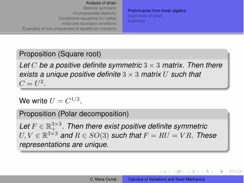
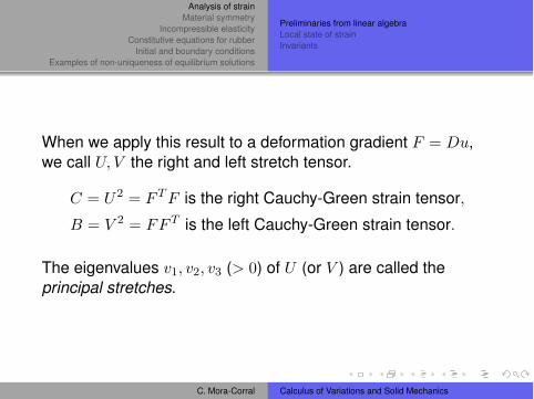
When we apply this result to a deformation gradient F = Du,we call U, V the right and left stretch tensor.
C = U2 = F T F is the right Cauchy-Green strain tensor,
B = V 2 = FF T is the left Cauchy-Green strain tensor.
The eigenvalues v1, v2, v3 (> 0) of U (or V ) are called theprincipal stretches.
C. Mora-Corral Calculus of Variations and Solid Mechanics
Analysis of strainMaterial symmetry
Incompressible elasticityConstitutive equations for rubber
Initial and boundary conditionsExamples of non-uniqueness of equilibrium solutions
Preliminaries from linear algebraLocal state of strainInvariants
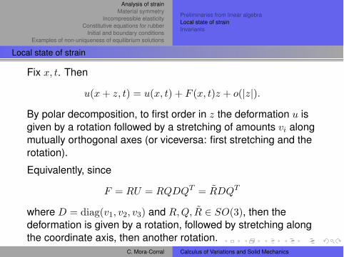
Local state of strain
Fix x, t. Then
u(x + z, t) = u(x, t) + F (x, t)z + o(|z|).
By polar decomposition, to first order in z the deformation u isgiven by a rotation followed by a stretching of amounts vi alongmutually orthogonal axes (or viceversa: first stretching and therotation).
Equivalently, since
F = RU = RQDQT = RDQT
where D = diag(v1, v2, v3) and R,Q, R " SO(3), then thedeformation is given by a rotation, followed by stretching alongthe coordinate axis, then another rotation.
C. Mora-Corral Calculus of Variations and Solid Mechanics
Analysis of strainMaterial symmetry
Incompressible elasticityConstitutive equations for rubber
Initial and boundary conditionsExamples of non-uniqueness of equilibrium solutions
Preliminaries from linear algebraLocal state of strainInvariants
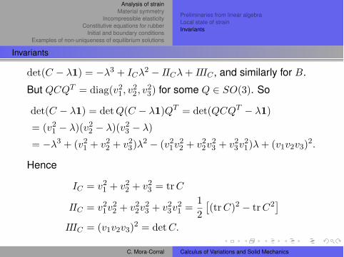
Invariants
det(C $ !1) = $!3 + IC!2 $ IIC! + IIIC , and similarly for B.
But QCQT = diag(v21, v
22, v
23) for some Q " SO(3). So
det(C $ !1) = det Q(C $ !1)QT = det(QCQT $ !1)
= (v21 $ !)(v2
2 $ !)(v23 $ !)
= $!3 + (v21 + v2
2 + v23)!
2 $ (v21v
22 + v2
2v23 + v2
3v21)! + (v1v2v3)2.
Hence
IC = v21 + v2
2 + v23 = trC
IIC = v21v
22 + v2
2v23 + v2
3v21 =
12
!(trC)2 $ trC2
"
IIIC = (v1v2v3)2 = detC.
C. Mora-Corral Calculus of Variations and Solid Mechanics
Analysis of strainMaterial symmetry
Incompressible elasticityConstitutive equations for rubber
Initial and boundary conditionsExamples of non-uniqueness of equilibrium solutions
Preliminaries from linear algebraLocal state of strainInvariants
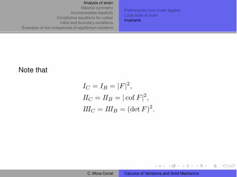
Note that
IC = IB = |F |2,IIC = IIB = | cof F |2,IIIC = IIIB = (detF )2.
C. Mora-Corral Calculus of Variations and Solid Mechanics
Analysis of strainMaterial symmetry
Incompressible elasticityConstitutive equations for rubber
Initial and boundary conditionsExamples of non-uniqueness of equilibrium solutions
Outline
1 Analysis of strain
2 Material symmetry
3 Incompressible elasticity
4 Constitutive equations for rubber
5 Initial and boundary conditions
6 Examples of non-uniqueness of equilibrium solutions
C. Mora-Corral Calculus of Variations and Solid Mechanics
Analysis of strainMaterial symmetry
Incompressible elasticityConstitutive equations for rubber
Initial and boundary conditionsExamples of non-uniqueness of equilibrium solutions
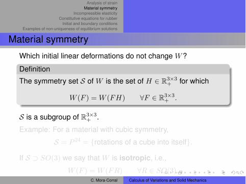
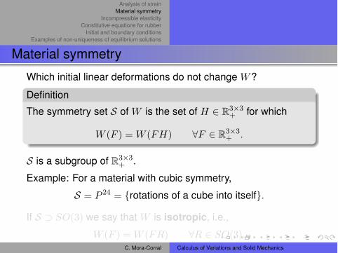
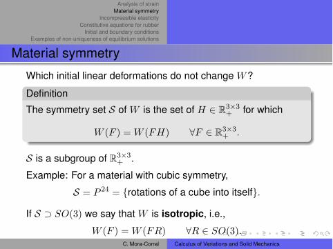
Material symmetry
Which initial linear deformations do not change W?
DefinitionThe symmetry set S of W is the set of H " R3!3
+ for which
W (F ) = W (FH) %F " R3!3+ .
S is a subgroup of R3!3+ .
Example: For a material with cubic symmetry,
S = P 24 = {rotations of a cube into itself}.
If S & SO(3) we say that W is isotropic, i.e.,
W (F ) = W (FR) %R " SO(3).C. Mora-Corral Calculus of Variations and Solid Mechanics
Analysis of strainMaterial symmetry
Incompressible elasticityConstitutive equations for rubber
Initial and boundary conditionsExamples of non-uniqueness of equilibrium solutions
Material symmetry
Which initial linear deformations do not change W?
DefinitionThe symmetry set S of W is the set of H " R3!3
+ for which
W (F ) = W (FH) %F " R3!3+ .
S is a subgroup of R3!3+ .
Example: For a material with cubic symmetry,
S = P 24 = {rotations of a cube into itself}.
If S & SO(3) we say that W is isotropic, i.e.,
W (F ) = W (FR) %R " SO(3).C. Mora-Corral Calculus of Variations and Solid Mechanics

Analysis of strainMaterial symmetry
Incompressible elasticityConstitutive equations for rubber
Initial and boundary conditionsExamples of non-uniqueness of equilibrium solutions
Examples of isotropic materials
Iron-Carbon alloy Galvanized steel Vulcanized rubber
C. Mora-Corral Calculus of Variations and Solid Mechanics
Analysis of strainMaterial symmetry
Incompressible elasticityConstitutive equations for rubber
Initial and boundary conditionsExamples of non-uniqueness of equilibrium solutions
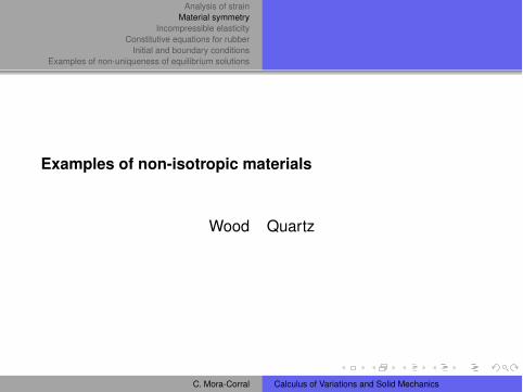
Examples of non-isotropic materials
Wood Quartz
C. Mora-Corral Calculus of Variations and Solid Mechanics
Analysis of strainMaterial symmetry
Incompressible elasticityConstitutive equations for rubber
Initial and boundary conditionsExamples of non-uniqueness of equilibrium solutions
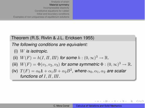
Theorem (R.S. Rivlin & J.L. Ericksen 1955)The following conditions are equivalent:
(i) W is isotropic.(ii) W (F ) = h(I, II, III) for some h : (0,')3 ( R.(iii) W (F ) = !(v1, v2, v3) for some symmetric ! : (0,')3 ( R.(iv) T (F ) = #01 + #1B + #2B2, where #0, #1, #2 are scalar
functions of I, II, III.
C. Mora-Corral Calculus of Variations and Solid Mechanics

Analysis of strainMaterial symmetry
Incompressible elasticityConstitutive equations for rubber
Initial and boundary conditionsExamples of non-uniqueness of equilibrium solutions
Outline
1 Analysis of strain
2 Material symmetry
3 Incompressible elasticity
4 Constitutive equations for rubber
5 Initial and boundary conditions
6 Examples of non-uniqueness of equilibrium solutions
C. Mora-Corral Calculus of Variations and Solid Mechanics
Analysis of strainMaterial symmetry
Incompressible elasticityConstitutive equations for rubber
Initial and boundary conditionsExamples of non-uniqueness of equilibrium solutions
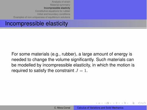
Incompressible elasticity
For some materials (e.g., rubber), a large amount of energy isneeded to change the volume significantly. Such materials canbe modelled by incompressible elasticity, in which the motion isrequired to satisfy the constraint J = 1.
C. Mora-Corral Calculus of Variations and Solid Mechanics
Analysis of strainMaterial symmetry
Incompressible elasticityConstitutive equations for rubber
Initial and boundary conditionsExamples of non-uniqueness of equilibrium solutions
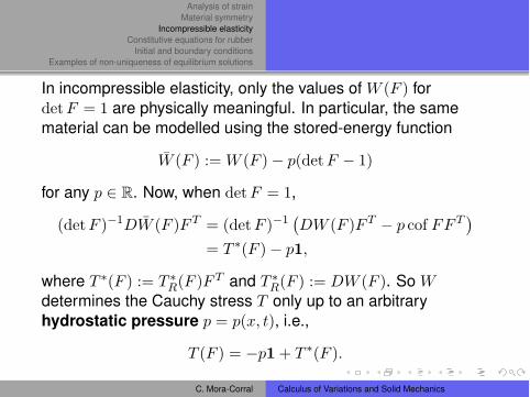
In incompressible elasticity, only the values of W (F ) fordet F = 1 are physically meaningful. In particular, the samematerial can be modelled using the stored-energy function
W (F ) := W (F )$ p(detF $ 1)
for any p " R. Now, when det F = 1,
(detF )"1DW (F )F T = (detF )"1#DW (F )F T $ p cof FF T
$
= T #(F )$ p1,
where T #(F ) := T #R(F )F T and T #R(F ) := DW (F ). So Wdetermines the Cauchy stress T only up to an arbitraryhydrostatic pressure p = p(x, t), i.e.,
T (F ) = $p1 + T #(F ).
C. Mora-Corral Calculus of Variations and Solid Mechanics
Analysis of strainMaterial symmetry
Incompressible elasticityConstitutive equations for rubber
Initial and boundary conditionsExamples of non-uniqueness of equilibrium solutions
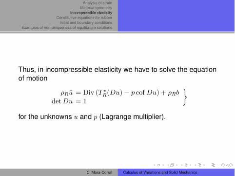
Thus, in incompressible elasticity we have to solve the equationof motion
$Ru = Div (T #R(Du)$ p cof Du) + $RbdetDu = 1
%
for the unknowns u and p (Lagrange multiplier).
C. Mora-Corral Calculus of Variations and Solid Mechanics
Analysis of strainMaterial symmetry
Incompressible elasticityConstitutive equations for rubber
Initial and boundary conditionsExamples of non-uniqueness of equilibrium solutions
Modelled as incompressibleModelled as compressible
Outline
1 Analysis of strain
2 Material symmetry
3 Incompressible elasticity
4 Constitutive equations for rubber
5 Initial and boundary conditions
6 Examples of non-uniqueness of equilibrium solutions
C. Mora-Corral Calculus of Variations and Solid Mechanics
Analysis of strainMaterial symmetry
Incompressible elasticityConstitutive equations for rubber
Initial and boundary conditionsExamples of non-uniqueness of equilibrium solutions
Modelled as incompressibleModelled as compressible
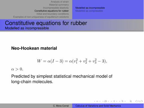
Constitutive equations for rubberModelled as incompressible
Neo-Hookean material
W = #(I $ 3) = #(v21 + v2
2 + v23 $ 3),
# > 0.
Predicted by simplest statistical mechanical model oflong-chain molecules.
C. Mora-Corral Calculus of Variations and Solid Mechanics
Analysis of strainMaterial symmetry
Incompressible elasticityConstitutive equations for rubber
Initial and boundary conditionsExamples of non-uniqueness of equilibrium solutions
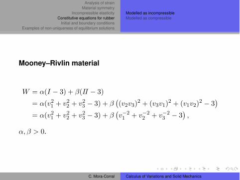
Modelled as incompressibleModelled as compressible
Mooney–Rivlin material
W = #(I $ 3) + %(II $ 3)
= #(v21 + v2
2 + v23 $ 3) + %
#(v2v3)2 + (v3v1)2 + (v1v2)2 $ 3
$
= #(v21 + v2
2 + v23 $ 3) + %
#v"21 + v"2
2 + v"23 $ 3
$,
#,% > 0.
C. Mora-Corral Calculus of Variations and Solid Mechanics
Analysis of strainMaterial symmetry
Incompressible elasticityConstitutive equations for rubber
Initial and boundary conditionsExamples of non-uniqueness of equilibrium solutions
Modelled as incompressibleModelled as compressible
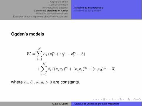
Ogden’s models
W =N&
i=1
#i (vpi1 + vpi
2 + vpi3 $ 3)
+M&
i=1
%i ((v2v3)qi + (v3v1)qi + (v1v2)qi $ 3)
where #i, %i, pi, qi > 0 are constants.
C. Mora-Corral Calculus of Variations and Solid Mechanics
Analysis of strainMaterial symmetry
Incompressible elasticityConstitutive equations for rubber
Initial and boundary conditionsExamples of non-uniqueness of equilibrium solutions
Modelled as incompressibleModelled as compressible
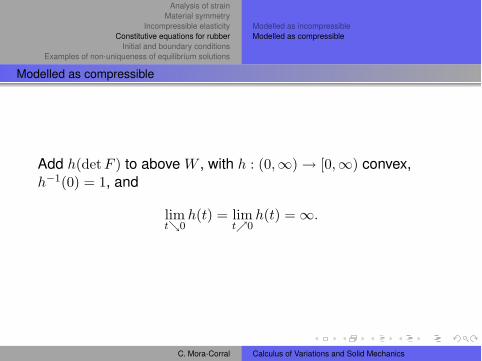
Modelled as compressible
Add h(det F ) to above W , with h : (0,')( [0,') convex,h"1(0) = 1, and
limt$0
h(t) = limt%0
h(t) ='.
C. Mora-Corral Calculus of Variations and Solid Mechanics
Analysis of strainMaterial symmetry
Incompressible elasticityConstitutive equations for rubber
Initial and boundary conditionsExamples of non-uniqueness of equilibrium solutions
Initial conditionsBoundary conditions
Outline
1 Analysis of strain
2 Material symmetry
3 Incompressible elasticity
4 Constitutive equations for rubber
5 Initial and boundary conditions
6 Examples of non-uniqueness of equilibrium solutions
C. Mora-Corral Calculus of Variations and Solid Mechanics
Analysis of strainMaterial symmetry
Incompressible elasticityConstitutive equations for rubber
Initial and boundary conditionsExamples of non-uniqueness of equilibrium solutions
Initial conditionsBoundary conditions
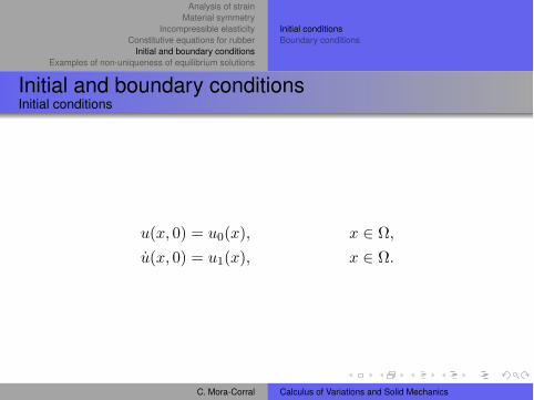
Initial and boundary conditionsInitial conditions
u(x, 0) = u0(x), x " ",
u(x, 0) = u1(x), x " ".
C. Mora-Corral Calculus of Variations and Solid Mechanics
Analysis of strainMaterial symmetry
Incompressible elasticityConstitutive equations for rubber
Initial and boundary conditionsExamples of non-uniqueness of equilibrium solutions
Initial conditionsBoundary conditions
Boundary conditions
(a) Displacement
u(x, t) = u(x, t) x " &".
(b) Dead load traction
TR(x, t)N(x) = sr(x, t), x " &".
The dead loads maintain the same direction and magnituteper unit reference area irrespective of the deformations.
(c) Pressure
T (u(x, t), t)n(u(x, t)) = $p(t)n(u(x, t)), x " &".
(d) Mixed boundary conditions combining the above.
C. Mora-Corral Calculus of Variations and Solid Mechanics
Analysis of strainMaterial symmetry
Incompressible elasticityConstitutive equations for rubber
Initial and boundary conditionsExamples of non-uniqueness of equilibrium solutions
Initial conditionsBoundary conditions
Boundary conditions
(a) Displacement
u(x, t) = u(x, t) x " &".
(b) Dead load traction
TR(x, t)N(x) = sr(x, t), x " &".
The dead loads maintain the same direction and magnituteper unit reference area irrespective of the deformations.
(c) Pressure
T (u(x, t), t)n(u(x, t)) = $p(t) n(u(x, t)), x " &".
(d) Mixed boundary conditions combining the above.
C. Mora-Corral Calculus of Variations and Solid Mechanics

Analysis of strainMaterial symmetry
Incompressible elasticityConstitutive equations for rubber
Initial and boundary conditionsExamples of non-uniqueness of equilibrium solutions
Outline
1 Analysis of strain
2 Material symmetry
3 Incompressible elasticity
4 Constitutive equations for rubber
5 Initial and boundary conditions
6 Examples of non-uniqueness of equilibrium solutions
C. Mora-Corral Calculus of Variations and Solid Mechanics

Analysis of strainMaterial symmetry
Incompressible elasticityConstitutive equations for rubber
Initial and boundary conditionsExamples of non-uniqueness of equilibrium solutions
Examples of non-uniqueness of equilibrium solutions
C. Mora-Corral Calculus of Variations and Solid Mechanics
Calculus of Variations and applications toSolid Mechanics
Carlos Mora-Corral
January 25–29 2010Lecture 4
C. Mora-Corral Calculus of Variations and Solid Mechanics

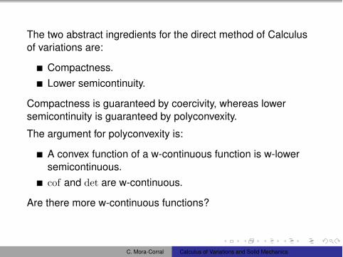
The two abstract ingredients for the direct method of Calculusof variations are:
Compactness.Lower semicontinuity.
Compactness is guaranteed by coercivity, whereas lowersemicontinuity is guaranteed by polyconvexity.
The argument for polyconvexity is:
A convex function of a w-continuous function is w-lowersemicontinuous.cof and det are w-continuous.
Are there more w-continuous functions?
C. Mora-Corral Calculus of Variations and Solid Mechanics
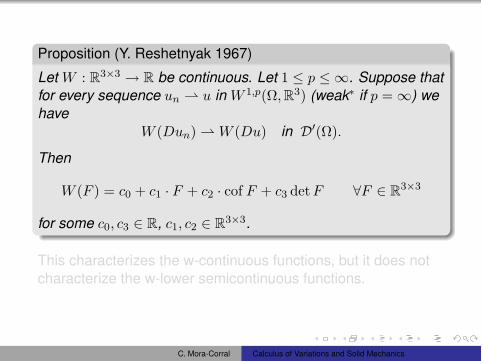
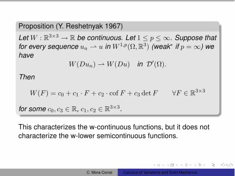
Proposition (Y. Reshetnyak 1967)
Let W : R3!3 ! R be continuous. Let 1 " p " #. Suppose thatfor every sequence un ! u in W 1,p(!, R3) (weak" if p =#) wehave
W (Dun) ! W (Du) in D#(!).
Then
W (F ) = c0 + c1 · F + c2 · cof F + c3 detF $F % R3!3
for some c0, c3 % R, c1, c2 % R3!3.
This characterizes the w-continuous functions, but it does notcharacterize the w-lower semicontinuous functions.
C. Mora-Corral Calculus of Variations and Solid Mechanics

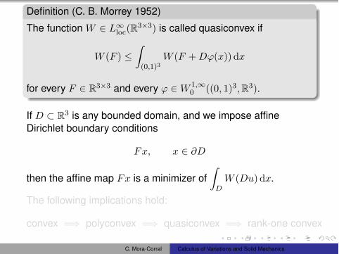
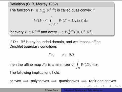
Definition (C. B. Morrey 1952)
The function W % L$loc(R3!3) is called quasiconvex if
W (F ) "!
(0,1)3W (F + D"(x)) dx
for every F % R3!3 and every " %W 1,$0 ((0, 1)3, R3).
If D & R3 is any bounded domain, and we impose affineDirichlet boundary conditions
Fx, x % #D
then the affine map Fx is a minimizer of!
DW (Du) dx.
The following implications hold:
convex =' polyconvex =' quasiconvex =' rank-one convex
C. Mora-Corral Calculus of Variations and Solid Mechanics
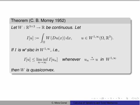
Theorem (C. B. Morrey 1952)
Let W : R3!3 ! R be continuous. Let
I[u] :=!
!W (Du(x)) dx, u %W 1,$(!, R3).
If I is w"slsc in W 1,$, i.e.,
I[u] " lim infn%$
I[un] whenever un"! u in W 1,$
then W is quasiconvex.
C. Mora-Corral Calculus of Variations and Solid Mechanics
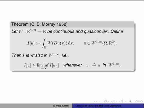
Theorem (C. B. Morrey 1952)
Let W : R3!3 ! R be continuous and quasiconvex. Define
I[u] :=!
!W (Du(x)) dx, u %W 1,$(!, R3).
Then I is w"slsc in W 1,$, i.e.,
I[u] " lim infn%$
I[un] whenever un"! u in W 1,$.
C. Mora-Corral Calculus of Variations and Solid Mechanics
The above results also hold for W 1,p, under natural growthconditions on W .
To sum up,
W quasiconvex ('!
!W (Du) dx weakly lower semicont.
This seems to solve completely the direct method of Calculusof Variations, and in a certain sense it does.
There is, however, a big difficulty. There is no tractablecondition for quasiconvexity. Quasiconvexity is only marginallymore transparent that lower semicontinuity itself.
The chain of implications
polyconvex =' quasiconvex =' rank-one convex
is greatly useful.
C. Mora-Corral Calculus of Variations and Solid Mechanics
Phase transformations in solidsInterfaces
Martensite to martensiteAustenite to martensite
MicrostructureShape-memory effect
Calculus of Variations and applications toSolid Mechanics
Carlos Mora-Corral
January 25–29 2010Lecture 5
C. Mora-Corral Calculus of Variations and Solid Mechanics
Phase transformations in solidsInterfaces
Martensite to martensiteAustenite to martensite
MicrostructureShape-memory effect
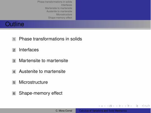
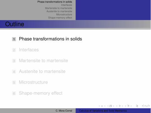
Outline
1 Phase transformations in solids
2 Interfaces
3 Martensite to martensite
4 Austenite to martensite
5 Microstructure
6 Shape-memory effect
C. Mora-Corral Calculus of Variations and Solid Mechanics
Phase transformations in solidsInterfaces
Martensite to martensiteAustenite to martensite
MicrostructureShape-memory effect
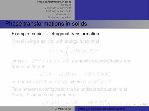
Phase transformations in solids
Example: cubic ! tetragonal transformation.
Model using elasticity with energy functional
I!(u) =!
!!(Du(x), ") dx,
where ! : R3!3 " (0,#)! R is smooth, bounded below andframe-indifferent:
!(F, ") = !(QF, ") $Q % SO(3),
and hence !(F, ") = !(U, "), where U = (F T F )1/2.
Take reference configuration to be undistorted austenite at" = "c. Assume cubic symmetry:
!(FR, ") = !(F, ") $R % P 24.C. Mora-Corral Calculus of Variations and Solid Mechanics

Phase transformations in solidsInterfaces
Martensite to martensiteAustenite to martensite
MicrostructureShape-memory effect
Phase transformations in solids
Example: cubic ! tetragonal transformation.
Model using elasticity with energy functional
I!(u) =!
!!(Du(x), ") dx,
where ! : R3!3 " (0,#)! R is smooth, bounded below andframe-indifferent:
!(F, ") = !(QF, ") $Q % SO(3),
and hence !(F, ") = !(U, "), where U = (F T F )1/2.
Take reference configuration to be undistorted austenite at" = "c. Assume cubic symmetry:
!(FR, ") = !(F, ") $R % P 24.C. Mora-Corral Calculus of Variations and Solid Mechanics
Phase transformations in solidsInterfaces
Martensite to martensiteAustenite to martensite
MicrostructureShape-memory effect
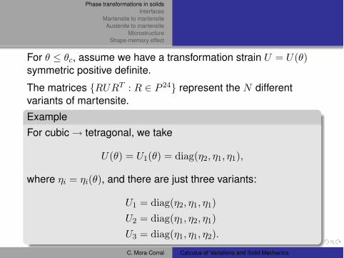
For " & "c, assume we have a transformation strain U = U(")symmetric positive definite.
The matrices {RURT : R % P 24} represent the N differentvariants of martensite.ExampleFor cubic ! tetragonal, we take
U(") = U1(") = diag(#2, #1, #1),
where #i = #i("), and there are just three variants:
U1 = diag(#2, #1, #1)U2 = diag(#1, #2, #1)U3 = diag(#1, #1, #2).
C. Mora-Corral Calculus of Variations and Solid Mechanics
Phase transformations in solidsInterfaces
Martensite to martensiteAustenite to martensite
MicrostructureShape-memory effect
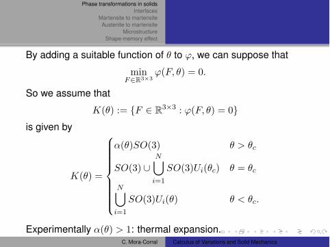
By adding a suitable function of " to !, we can suppose that
minF"R3!3
!(F, ") = 0.
So we assume that
K(") := {F % R3!3 : !(F, ") = 0}is given by
K(") =
"#######$
#######%
$(")SO(3) " > "c
SO(3) 'N&
i=1
SO(3)Ui("c) " = "c
N&
i=1
SO(3)Ui(") " < "c.
Experimentally $(") > 1: thermal expansion.C. Mora-Corral Calculus of Variations and Solid Mechanics
Phase transformations in solidsInterfaces
Martensite to martensiteAustenite to martensite
MicrostructureShape-memory effect
Outline
1 Phase transformations in solids
2 Interfaces
3 Martensite to martensite
4 Austenite to martensite
5 Microstructure
6 Shape-memory effect
C. Mora-Corral Calculus of Variations and Solid Mechanics
Phase transformations in solidsInterfaces
Martensite to martensiteAustenite to martensite
MicrostructureShape-memory effect
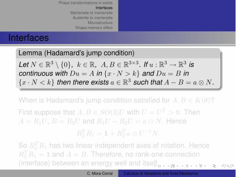
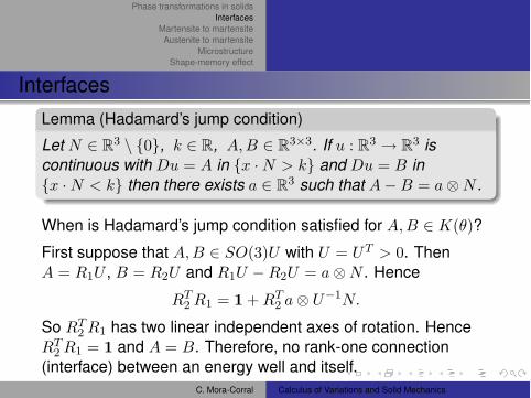
InterfacesLemma (Hadamard’s jump condition)
Let N % R3 \ {0}, k % R, A, B % R3!3. If u : R3 ! R3 iscontinuous with Du = A in {x · N > k} and Du = B in{x · N < k} then there exists a % R3 such that A(B = a)N .
When is Hadamard’s jump condition satisfied for A, B % K(")?
First suppose that A, B % SO(3)U with U = UT > 0. ThenA = R1U , B = R2U and R1U (R2U = a)N . Hence
RT2 R1 = 1 + RT
2 a) U#1N.
So RT2 R1 has two linear independent axes of rotation. Hence
RT2 R1 = 1 and A = B. Therefore, no rank-one connection
(interface) between an energy well and itself.C. Mora-Corral Calculus of Variations and Solid Mechanics
Phase transformations in solidsInterfaces
Martensite to martensiteAustenite to martensite
MicrostructureShape-memory effect
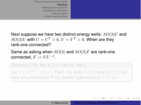
Next suppose we have two distinct energy wells: SO(3)U andSO(3)V with U = UT > 0, V = V T > 0. When are theyrank-one connected?
Same as asking when SO(3) and SO(3)F are rank-oneconnected, F := V U#1.
Theorem (J.M. Ball & R.D. James 1987)
Let F % R3!3+ \ SO(3). Then, the wells SO(3) and SO(3)F are
rank-one connected iff the middle eigenvalue of F T F is 1.
C. Mora-Corral Calculus of Variations and Solid Mechanics

Phase transformations in solidsInterfaces
Martensite to martensiteAustenite to martensite
MicrostructureShape-memory effect
Next suppose we have two distinct energy wells: SO(3)U andSO(3)V with U = UT > 0, V = V T > 0. When are theyrank-one connected?
Same as asking when SO(3) and SO(3)F are rank-oneconnected, F := V U#1.
Theorem (J.M. Ball & R.D. James 1987)
Let F % R3!3+ \ SO(3). Then, the wells SO(3) and SO(3)F are
rank-one connected iff the middle eigenvalue of F T F is 1.
C. Mora-Corral Calculus of Variations and Solid Mechanics
Phase transformations in solidsInterfaces
Martensite to martensiteAustenite to martensite
MicrostructureShape-memory effect
Outline
1 Phase transformations in solids
2 Interfaces
3 Martensite to martensite
4 Austenite to martensite
5 Microstructure
6 Shape-memory effect
C. Mora-Corral Calculus of Variations and Solid Mechanics
Phase transformations in solidsInterfaces
Martensite to martensiteAustenite to martensite
MicrostructureShape-memory effect
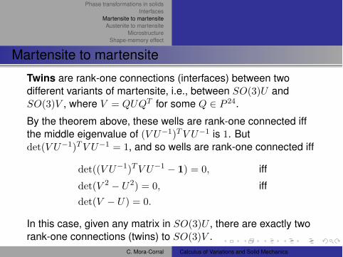
Martensite to martensite
Twins are rank-one connections (interfaces) between twodifferent variants of martensite, i.e., between SO(3)U andSO(3)V , where V = QUQT for some Q % P 24.
By the theorem above, these wells are rank-one connected iffthe middle eigenvalue of (V U#1)T V U#1 is 1. Butdet(V U#1)T V U#1 = 1, and so wells are rank-one connected iff
det((V U#1)T V U#1 ( 1) = 0, iffdet(V 2 ( U2) = 0, iffdet(V ( U) = 0.
In this case, given any matrix in SO(3)U , there are exactly tworank-one connections (twins) to SO(3)V .
C. Mora-Corral Calculus of Variations and Solid Mechanics
Phase transformations in solidsInterfaces
Martensite to martensiteAustenite to martensite
MicrostructureShape-memory effect
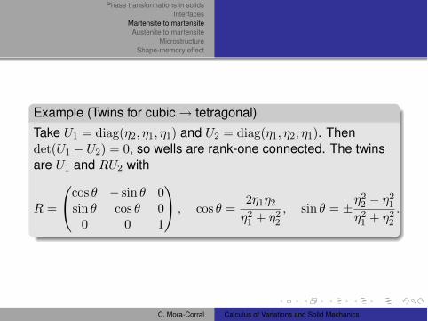
Example (Twins for cubic ! tetragonal)Take U1 = diag(#2, #1, #1) and U2 = diag(#1, #2, #1). Thendet(U1 ( U2) = 0, so wells are rank-one connected. The twinsare U1 and RU2 with
R =
'
(cos " ( sin " 0sin " cos " 0
0 0 1
)
* , cos " =2#1#2
#21 + #2
2
, sin " = ±#22 ( #2
1
#21 + #2
2
.
C. Mora-Corral Calculus of Variations and Solid Mechanics

Phase transformations in solidsInterfaces
Martensite to martensiteAustenite to martensite
MicrostructureShape-memory effect
Outline
1 Phase transformations in solids
2 Interfaces
3 Martensite to martensite
4 Austenite to martensite
5 Microstructure
6 Shape-memory effect
C. Mora-Corral Calculus of Variations and Solid Mechanics
Phase transformations in solidsInterfaces
Martensite to martensiteAustenite to martensite
MicrostructureShape-memory effect
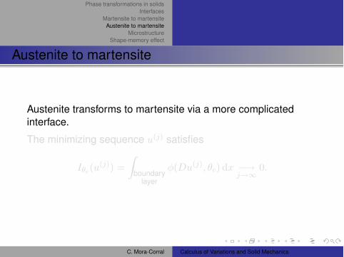
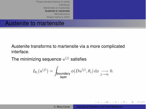
Austenite to martensite
Austenite transforms to martensite via a more complicatedinterface.
The minimizing sequence u(j) satisfies
I!c(u(j)) =
!
boundarylayer
%(Du(j), "c) dx (!j$%
0.
C. Mora-Corral Calculus of Variations and Solid Mechanics
Phase transformations in solidsInterfaces
Martensite to martensiteAustenite to martensite
MicrostructureShape-memory effect
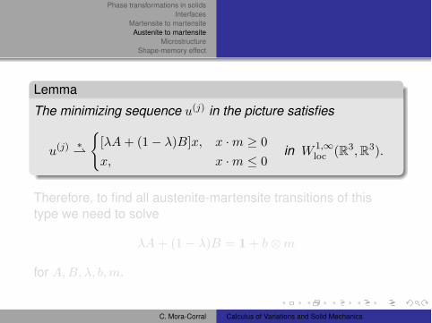
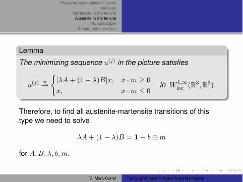
Lemma
The minimizing sequence u(j) in the picture satisfies
u(j) &&
+['A + (1( ')B]x, x · m * 0x, x · m & 0
in W 1,%loc (R3, R3).
Therefore, to find all austenite-martensite transitions of thistype we need to solve
'A + (1( ')B = 1 + b)m
for A, B, ', b, m.
C. Mora-Corral Calculus of Variations and Solid Mechanics
Phase transformations in solidsInterfaces
Martensite to martensiteAustenite to martensite
MicrostructureShape-memory effect
Lemma
The minimizing sequence u(j) in the picture satisfies
u(j) &&
+['A + (1( ')B]x, x · m * 0x, x · m & 0
in W 1,%loc (R3, R3).
Therefore, to find all austenite-martensite transitions of thistype we need to solve
'A + (1( ')B = 1 + b)m
for A, B, ', b, m.
C. Mora-Corral Calculus of Variations and Solid Mechanics

Phase transformations in solidsInterfaces
Martensite to martensiteAustenite to martensite
MicrostructureShape-memory effect
Outline
1 Phase transformations in solids
2 Interfaces
3 Martensite to martensite
4 Austenite to martensite
5 Microstructure
6 Shape-memory effect
C. Mora-Corral Calculus of Variations and Solid Mechanics
Phase transformations in solidsInterfaces
Martensite to martensiteAustenite to martensite
MicrostructureShape-memory effect
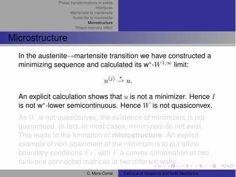
Microstructure
In the austenite!martensite transition we have constructed aminimizing sequence and calculated its w&-W 1,% limit:
u(j) && u.
An explicit calculation shows that u is not a minimizer. Hence Iis not w&-lower semicontinuous. Hence W is not quasiconvex.
As W is not quasiconvex, the existence of minimizers is notguaranteed. In fact, in most cases, minimizers do not exist.This leads to the formation of microstructure. An explicitexample of non-attainment of the minimum is to put affineboundary conditions Fx, with F a convex combination of tworank-one connected matrices in two different wells.
C. Mora-Corral Calculus of Variations and Solid Mechanics
Phase transformations in solidsInterfaces
Martensite to martensiteAustenite to martensite
MicrostructureShape-memory effect
Microstructure
In the austenite!martensite transition we have constructed aminimizing sequence and calculated its w&-W 1,% limit:
u(j) && u.
An explicit calculation shows that u is not a minimizer. Hence Iis not w&-lower semicontinuous. Hence W is not quasiconvex.
As W is not quasiconvex, the existence of minimizers is notguaranteed. In fact, in most cases, minimizers do not exist.This leads to the formation of microstructure. An explicitexample of non-attainment of the minimum is to put affineboundary conditions Fx, with F a convex combination of tworank-one connected matrices in two different wells.
C. Mora-Corral Calculus of Variations and Solid Mechanics

Phase transformations in solidsInterfaces
Martensite to martensiteAustenite to martensite
MicrostructureShape-memory effect
Since minimizers do not exist, the right object to study in orderto understand the “minimum” are the minimizing sequences.
(The mathematical theory of Young measures can also be used tounderstand the “minimum”).
Minimizing sequences predict infinitely fine microstruture. Inpractise, the microstructure is extremely fine but not infinitelyfine. The microstructure can be as fine as 6 atoms wide.
C. Mora-Corral Calculus of Variations and Solid Mechanics
Phase transformations in solidsInterfaces
Martensite to martensiteAustenite to martensite
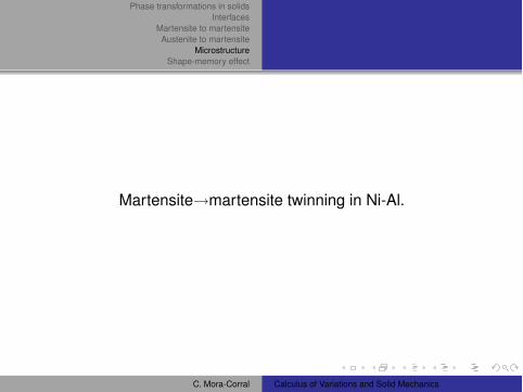
MicrostructureShape-memory effect
Martensite!martensite twinning in Ni-Al.
C. Mora-Corral Calculus of Variations and Solid Mechanics
Phase transformations in solidsInterfaces
Martensite to martensiteAustenite to martensite
MicrostructureShape-memory effect
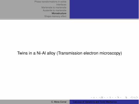
Twins in a Ni-Al alloy (Transmission electron microscopy)
C. Mora-Corral Calculus of Variations and Solid Mechanics

Phase transformations in solidsInterfaces
Martensite to martensiteAustenite to martensite
MicrostructureShape-memory effect
Austenite!martensite interface in Cu82.5Al14.0Ni3.5
C. Mora-Corral Calculus of Variations and Solid Mechanics

Phase transformations in solidsInterfaces
Martensite to martensiteAustenite to martensite
MicrostructureShape-memory effect
Outline
1 Phase transformations in solids
2 Interfaces
3 Martensite to martensite
4 Austenite to martensite
5 Microstructure
6 Shape-memory effect
C. Mora-Corral Calculus of Variations and Solid Mechanics

Phase transformations in solidsInterfaces
Martensite to martensiteAustenite to martensite
MicrostructureShape-memory effect
Shape-memory effect
The wire is initially martensite. As you bend it, themicrostructure changes to accommodate the bending, withoutdamage to the material. When heating above "c the minimumenergy is given by
Du(x) % $(")SO(3) $x % !,
which implies (J. Liouville 1850)
Du(x) = $(")R $x % !
for some constant R % SO(3).
C. Mora-Corral Calculus of Variations and Solid Mechanics

Phase transformations in solidsInterfaces
Martensite to martensiteAustenite to martensite
MicrostructureShape-memory effect
Conclusion
The shape-memory effect is an exceptional phenomenom.Currently, about 30 such metal alloys are known, of which about15 have industrial applications: Cu-Al-Ni, Al-Ni-Ti, Mn-Cu. . .
Mathematically, this exceptionality is given by the followingnecessary conditions on W for the shape-memory effect to takeplace:
1 W is not quasiconvex.2 W has one well at high temperatures, and several wells at
low temperatures.3 The martensitic wells are rank-one connected (middle
eigenvalue 1 condition).
C. Mora-Corral Calculus of Variations and Solid Mechanics
Phase transformations in solidsInterfaces
Martensite to martensiteAustenite to martensite
MicrostructureShape-memory effect
Experimentally, eigenvalues in [0.99, 1.01] are OK, but notoutside this range. It is the possibility of the fine tuning ofpercentages in alloys that allows (some of) them to reach theeigenvalue 1 condition: Cu69.0Al27.5Ni3.5, Ni30.5Ti49.5Cu20.0,Cu68Zn15Al17. . .
C. Mora-Corral Calculus of Variations and Solid Mechanics
Phase transformations in solidsInterfaces
Martensite to martensiteAustenite to martensite
MicrostructureShape-memory effect
Industrial applications
Medicine, Orthodontics.Couplings (between two vehicles, two pipes. . . ).Automobile: Transmission fluid control, sealinghigh-pressure fuel passages in diesel engine injectors.Cellular phone antenna.Eyeglass frames.
C. Mora-Corral Calculus of Variations and Solid Mechanics