calibration of pod reduced-order models using tikhonov

INTERNATIONAL JOURNAL FOR NUMERICAL METHODS IN FLUIDSInt. J. Numer. Meth. Fluids 2009; 00:1–00 Prepared using fldauth.cls [Version: 2002/09/18 v1.01]

Calibration of POD Reduced-Order Models using Tikhonovregularization

L. Cordier1,∗, B. Abou El Majd1 and J. Favier2

1 LEA - CEAT, 43, rue de l’Aérodrome, 86036 Poitiers Cedex, France2 DICAT, University of Genova, via Montallegro 1, 16145 Genova, Italy

SUMMARY

In this paper we compare various methods of calibration that can be used in practice to improvethe accuracy of reduced-order models based on Proper Orthogonal Decomposition. The bench markconfiguration retained corresponds to a case of relatively simple dynamics: a two-dimensional flowaround a cylinder for a Reynolds number of 200. We generalize to the first and second-order themethod of calibration based on Tikhonov regularization recently used in [1]. Finally, we show that forthis flow configuration this procedure is the most effective in terms of reduction of errors. Copyrightc© 2009 John Wiley & Sons, Ltd.

key words: POD Reduced Order Model ; Calibration ; Tikhonov regularization ; Optimization

1. INTRODUCTION

Within a relatively short period of a few years, reduced-order modeling by Proper OrthogonalDecomposition (POD) has gained a significant importance in fluid mechanics and turbulence.This sudden increase of interest is mainly linked to recent developments of technologicalfacilities (computers, data acquisition systems) which now allow easier and faster datarecording, ready-to-use for the POD (space-time correlations). However, in the majority of theapplications, the studies are not carried out up to a complete and accurate representation of theflow dynamics by POD, even if the procedure is now well-known. The latter requires a Galerkinprojection of the governing equations (in general the Navier-Stokes equations) onto the spatialPOD functions, to obtain after truncation in the POD subspace, a set of ordinary differentialequations representing the dynamics of the original system. Then, how can we explain thatthe most promising approaches in terms of applications: optimization and optimal controlproblems, real-time flow control, parametric studies, continuation methods,. . . are hardly usedin the literature? The major barrier to the expansion of POD Galerkin approach is essentiallythe lack of accuracy of the reduced-order models obtained. Indeed, it is often difficult to

∗Correspondence to: LEA - CEAT, 43, rue de l’Aérodrome, 86036 Poitiers Cedex, [email protected]

Copyright c© 2009 John Wiley & Sons, Ltd.

2 L. CORDIER, B. ABOU EL MAJD AND J. FAVIER

represent with a sufficient accuracy, the dynamics at short times of the original system withthe parameters of control used to determine the POD basis. In these conditions, what canbe expected from the ability of POD-based reduced-order models to represent the dynamicsof the system at long times (bifurcation studies, for instance) or to predict the dynamics ofthe system for parameters of control different from those used to determine the POD basis(flow control applications)? Recently, various studies [2, 3, 4, 5, 6, 7], presenting numericalmethods termed as calibration, appeared in the literature in order to improve the accuracyof POD-based reduced-order models thanks to solutions of optimization problems. The ideais simple, since the temporal dynamics of the POD model is known in advance, it is possibleto use this information to correct whole or part of the coefficients issued from POD Galerkin.However, according to our knowledge of the literature, there is no trace of any comparativestudy of these methods. It is then difficult to claim which is the most effective method in termsof reduction of errors. The initial objective of this paper is to use a bench mark configuration,simple from the point of view of dynamics, to analyze thoroughly these various approaches,and, if possible, to release a more effective strategy. Incidentally, this approach led us to extendthe method of calibration based on Tikhonov regularization [8] recently used in [1] to the firstand second-order [9].

This manuscript is organized as follows. Section 2.1 introduces the Proper OrthogonalDecomposition in the general context of approximation functions. Then, the POD Galerkinapproach is described for a generic controlled flow configuration (section 2.2.1). In the nextsubsection (section 2.2.2), the equations of the reduced-order model based on POD aresimplified in order to give an overall picture of the methods of calibration. In section 2.3,the bench mark flow configuration used in this study is first described, then the necessity ofintroducing methods of calibration to improve the accuracy of the POD model is motivated.Section 3 is dedicated to the presentation of the existing methods of calibration, within anunified framework. The various choices of definitions of errors between the calibrated dynamicsand that of the original system are first presented in section 3.1. Then, we show in section3.2 that in the case of affine functions of errors, the minimization of the normalized errorsleads to the resolution of a linear system. To conclude section 3, the method of calibrationsuggested in [3] is presented in section 3.3. The various methods of calibration used so far inthe literature are then compared on the bench mark configuration in section 4. Finally, weintroduce in section 5 the method of calibration based on the Tikhonov regularization, whichwe have developed in this paper, and present the results of a comparative study to determinethe most effective method of calibration.

2. REDUCED-ORDER MODELING BASED ON A POD GALERKIN APPROACH

2.1. Proper Orthogonal Decomposition

Given a set of data, elements of a high dimensional space (potentially infinite), the mainidea of the Proper Orthogonal Decomposition (POD) is to determine a subspace of reduceddimension which is optimal in the sense that the error of projection on this subspaceis minimal. To formulate this statement more precisely, we introduce H a Hilbert spacewith inner product (·, ·)H and induced norm ‖ · ‖H . In the majority of the applications,and it will be our case besides, H corresponds to L2(Ω), with Ω the spatial domain. Let

Copyright c© 2009 John Wiley & Sons, Ltd. Int. J. Numer. Meth. Fluids 2009; 00:1–0Prepared using fldauth.cls

CALIBRATION OF POD ROM USING TIKHONOV REGULARIZATION 3

U = u(x, tm) = umm=1,...,Ntbe a set of Nt snapshots taken over a time interval [0, T ], with

x ∈ Ω. Then, the aim of the POD is to find a subspace S of dimension NPOD ≪ Nt, such thatthe error E (‖u− PSu‖H) is minimized†. Here, E (·) denotes an average operator over m, for

instance an ensemble average (E (u) = 1Nt

∑Nt

m=1 um), and PS the orthogonal projection ontoS. The procedure is then equivalent to minimize the expression

1

Nt

Nt∑

m=1

∥∥∥∥um − PSum

∥∥∥∥

2

H

=1

Nt

Nt∑

m=1

∥∥∥∥um −

NPOD∑

j=1

aPj (tm)Φj

∥∥∥∥

2

H

,

where Φjj=1,...,NPODis a basis for the subspace S and aP

j j=1,...,NPODrefer to temporal

coefficients corresponding to the POD expansion (as indicated by the superscript P ). It canbe shown ([10] or [11] for instance) that this minimization problem leads to the eigenvalueproblem:

RΦj = λjΦj j = 1, · · · , NPOD,

where R = E (u⊗ u∗). Here, ⊗ denotes the dyadic product between two vectors u and u∗

where the ∗ superscript indicates complex conjugate.Since R is linear, self-adjoint and positive semi-definite on H , the spectral theory applies

and guarantees that:

1. we may choose Φj to be orthonormal, i.e. aPj (tm) = (um,Φj),

2. we have λ1 ≥ λ2 ≥ · · · ≥ λNPOD≥ 0 where λj (j = 1, · · · , NPOD) are the largest NPOD

eigenvalues of R.

This approach is called direct method and corresponds to the formulation introducedoriginally in [12]. However, when the input data come from numerical simulations, it is muchmore efficient to use an alternate way of computing the POD eigenfunctions. This method,known as method of snapshots [13], consists of writing the POD modes as linear combinationsof the snapshots:

Φj(x) =

Nt∑

m=1

bmj um(x).

The vectors bj =(

b1j , · · · , bNt

j

)T

are then determined as the solutions of a new eigenvalue

problem given by:

Cbj = λjbj ,

where C is a Nt × Nt correlation matrix with Cij = 1Nt

(ui,uj

). This matrix is self-adjoint, as

for the direct method. It follows that the vectors bj are orthogonal with respect to the innerproduct defined by:

(bj ,bk)T

=1

Nt

Nt∑

m=1

bmj bm

k .

†Remind that for any orthogonal projection PS we have ‖u‖2H = ‖u − PSu‖2

H + ‖PSu‖2H . Then, minimizing

E(‖u − PSu‖2

H

)is equivalent to maximizing E

(‖PSu‖2

H

).



By extension, the inner product associated with the direct method will henceforth be denoted(Φj ,Φk)Ω where by definition:

(Φj ,Φk)Ω =

∫

Ω

Φj(x) · Φk(x) dx,

with · the notation of the standard Euclidean inner product.

2.2. POD Reduced-Order Model based on Galerkin projection

2.2.1. General description For incompressible flows, the motion of the fluid is described bythe incompressibility condition and the Navier-Stokes equations,

∇ · u = 0,

∂tu = N (u) −∇p with N (u) = − (u · ∇)u +1

Re∆u.

In these equations, all variables (u velocity vector and p pressure) are assumed to be non-dimensional and Re is the Reynolds number.

The POD Reduced-Order Model (POD ROM) is then constructed by applying the Galerkinprojection to the governing equations. Since by construction the eigenfunctions Φi aredivergence-free for an incompressible flow, they can be used as test functions to derive thevariational formulation of the Navier-Stokes equations:

(∂tu,Φi)Ω = (N (u),Φi)Ω − (∇p,Φi)Ω . (1)

Using the relation ∇ · Φi = 0, the pressure term can be rewritten as a boundary term:

(∇p,Φi)Ω =

∫

Ω

Φi · ∇p dx =

∫

Ω

∇ · (pΦi) dx =

∫

∂Ω

pΦi · n dx = Pi,

where n is the outward unit normal at the boundary surface ∂Ω. If the snapshots um employedfor the POD are zero on the boundary, then Φi = 0 on ∂Ω and the pressure term vanishes. Inmost of the applications [14, 2, 4], the contribution of the pressure term is simply neglected asa first approximation.

To carry on our developments, we have to specify the variable on which the POD will beapplied. Beyond the idea of a correct representation of the flow physics, we would like tosimplify as much as possible the analytical expressions of the coefficients associated to thePOD ROM. In the previous paragraph, we point out that prescribing Φi = 0 on the boundaryis relevant for the pressure term. We will thus use a lifting procedure discussed thoroughlyin [15]: if the boundary conditions are time-independent (uncontrolled flow for instance), theoriginal set of snapshots U is replaced by U ′ = um − umm=1,...,Nt

where um = E(u); if theboundary conditions are time-dependent (flow controlled at the boundary for instance), thePOD is applied to U ′′ = um−γmuc−umm=1,...,Nt

where γm = γ(tm) characterizes the timeevolution of the control and uc is the actuation mode. In practice, this mode is determinedas a particular solution of the Navier-Stokes equations, where the boundary conditions on thecontrolled part of ∂Ω are equal to the spatial evolution of the control, and where the boundaryconditions on the uncontrolled part are set to zero (see [16] for an application to the controlledcylinder wake).



In the general formulation, the velocity expansion of u over the POD modes Φj writes:

u(x, t) = um(x) + γ(t)uc(x) +

NPOD∑

j=1

aj(t)Φj(x). (2)

By substituting (2) into the Galerkin projection (1), we obtain after some algebraicmanipulations [17] the following expression for the reduced-order model in the presence ofcontrol:

aRi (t) = AGP

i + BGPij aR

j (t) + CGPijk aR

j (t)aRk (t) − Pi(t) (3a)

+DGPi γ(t) +

(

EGPi + FGP

ij aRj (t)

)

γ(t) + GGPi γ2(t)

aRi (0) = aP

i (0) = (u(x, 0) − um(x) − γ(0)uc(x),Φi)Ω , (3b)

where the Einstein summation is used and all subscripts i, j, k run from 1 to Ngal. Here,Ngal < NPOD corresponds to the number of Galerkin modes retained in the reduced-ordermodel. This number of modes is assumed to be sufficient to reproduce accurately the flow (seesection 2.3 to evaluate Ngal). The coefficients AGP

i , BGPij , CGP

ijk , DGPi , EGP

i , FGPij and GGP

i

depend explicitly on Φ, um and uc (see Appendix I). The superscripts R are introduced forthe temporal coefficients ai are to indicate that these coefficients are obtained by integrating intime the system of ODEs (3). Similarly, we introduce the superscripts GP for the coefficientsof the POD ROM to stress that these coefficients are obtained directly by Galerkin projection.

2.2.2. Simplification of the POD ROM In practice, the POD ROM (3) will not necessarily beintegrated in time with the coefficients determined by the method of POD Galerkin. Indeed,whole or part of the coefficients may either be unknown (in the case of experimental data forinstance) or known with an insufficient level of accuracy to reproduce correctly the originaldynamics (see section 2.3 for an example). It is thus necessary to identify, or in other wordscalibrate, whole or part of the coefficients. Since the structure of (3a) is not modified by thepressure term [18], we can consider without restricting the generality Pi(t) = 0.

In section 3, the various methods of calibration encountered in the literature will be presented

within a unified framework. Therefore we introduce aR(t) =(

aR1 (t), · · · , aR

Ngal(t)

)T

, vectorial

solution of (3), to rewrite compactly (3a) as:

aRi (t) = fi(yi,a

R(t)) + gi(zi,aR(t), γ) i = 1, · · · , Ngal, (4a)

where fi(yi,aR(t)) = Ai + Bij aR

j (t) + Qijk aRj (t)aR

k (t), (4b)

and gi(zi,aR(t), γ) = Di γ(t) +

(

Ei + Fij aRj (t)

)

γ(t) + Giγ2(t) (4c)

with j = 1, · · · , Ngal and k = 1, · · · , j. In (4a), yi and zi denote the unknown coefficientscorresponding to respectively the uncontrolled and controlled part of (3a), i.e.



yi =

Ai

Bi1

...BiNgal

Qi11

...QiNgalNgal

∈ RNyi and zi =

Di

Ei

Fi1

...FiNgal

Gi

∈ RNzi ,

where Nyi= 1+Ngal+

Ngal(Ngal+1)2 and Nzi

= 3+Ngal. In (4b), the coefficients Qijk correspondto the symmetric part of Cijk only, i.e. Qijk = 1/2 (Cijk + Cikj) for i, j = 1, · · · , Ngal andk = 1, · · · , j. This modification of the expression of the quadratic term is justified by the factthat it is impossible to differentiate Cijk from Cikj by any technique of calibration.

In vectorial formulation, the controlled POD ROM given by (4a) is finally:

aR(t) = f(y,aR(t)) + g(z,aR(t), γ), (5)

where for the uncontrolled contribution:

f =

f1

f2

...fNgal

∈ RNgal ; y =

y1

y2

...yNgal

∈ RNy with Ny = NgalNyi

,

and, for the controlled contribution:

g =

g1

g2

...gNgal

∈ RNgal ; z =

z1

z2

...zNgal

∈ RNz with Nz = NgalNzi

.

Here, f and g can be evaluated easily using the coefficients of the model y and z (seeAppendix II).

For the sake of clarity, the rest of the paper is limited to uncontrolled flows, i.e. γ = 0 org = 0, in (5). One of the interests of (5) is to clearly demonstrate that for a given value ofγ the extension to controlled flows is straightforward (see [1] for a recent application of thecalibration techniques to a controlled wake flow).

2.3. Two-dimensional cylinder wake flow at Re = 200

The reduced-order modeling approach based on POD is now applied to a two-dimensionalincompressible cylinder wake flow at Re = 200. The database was computed using a finite-element code (DNS code Icare, IMFT/University of Toulouse, see [19] for details) and containsNt = 200 two-dimensional snapshots of the flow velocity, taken over a period T = 12 i.e. overmore than two periods of vortex shedding (Tvs = 5). Typical iso-values of the longitudinal



Figure 1. Iso-values of the longitudinal velocity fluctuation.

velocity are shown in Fig. 1.

Following the discussion of section 2.2.1, the method of snapshots introduced in section 2.1is applied to the velocity fluctuation. The first six spatial eigenfunctions Φi are represented inFig. 2 and the relative kinetic energy is plotted in logarithmic scale for the first 40 POD modesin Fig. 3. The energy is clearly concentrated in a very small number of modes: the first sixPOD modes are sufficient to represent 99.9% of the flow energy and we thus consider Ngal = 6to derive the POD ROM.

The POD ROM (5) is then integrated in time with a classical fourth-order Runge-Kuttascheme and a time step of 10−3T . A set of predicted time histories for the mode amplitudesaR

i (t) is obtained, and compared to the set of POD temporal eigenfunctions aPi (t). As shown in

Fig. 4, the original dynamics is globally well reproduced but the accuracy is not perfect. Indeed,the most energetic mode is well reconstructed, while for the higher modes the maxima remainover-estimated. Besides that, a constant phase shift can quickly occur between the dynamicsof the model and that of the original one (see mode 3 for instance). If the final objective is touse the POD ROM in a phase control strategy, then these errors can lead to the failure of thiscontrol strategy. This relatively bad performances of the model may be attributed to

i) the structural instability of the Galerkin projection [20, 21, 14],ii) the truncation of the POD basis (dissipative scales associated to higher POD modes are

not sufficiently present in the model),iii) the fact that the set of data does not perfectly respect the weak formulation

(5): inaccurate treatment of the boundary terms and the pressure contribution,incompressibility not verified (experimental data),

iv) an insufficient numerical precision to compute the POD ROM coefficients.

It is thus necessary to introduce calibration techniques in order to reproduce accurately thedynamics of reference using the POD ROM.



(a) Mode 1. (b) Mode 2.

(c) Mode 3. (d) Mode 4.

(e) Mode 5. (f) Mode 6.

Figure 2. The first 6 spatial POD eigenfunctions are visualized by iso-values of their norm (‖Φi‖Ω).

3. EXISTING CALIBRATION METHODS

Many methods of calibration have already been proposed in the literature. Let us quote forexample the different techniques based on least-square minimization [2, 3, 5], those consistingin solving a constrained optimization problem, iteratively [22] or simultaneously [6], the recentmethod termed intrinsic stabilization introduced in [7], and finally the calibration proceduresuggested by [3]. To compare fairly the previous procedures on the case of the cylinder wakeflow (see section 4), we first introduce various criteria of error (section 3.1), along the lines of[3]. Then, we emphasize in section 3.2 that the problem of minimization reduces to a linearsystem when the errors are affine functions of y. Finally, the calibration procedure suggestedin [3] is presented, as the Tikhonov regularization method proposed in this paper (section 5)constitutes an alternative to their approach.



0 2 4 6 8 10 12 14 16 18 20 22 24 26 28 30 32 34 36 38 401e-05

0.0001

0.001

0.01

0.1

1

10

100

12

3456

POD index number i

λi/E

Nt

Figure 3. POD eigenvalues in logarithmic scale. ENt corresponds to twice the energy contained in the

database (ENt =∑Nt

j=1 λj).

t

a1

0

0

1

1

2

2

3

3

4

4

5 6

−1

−2

−3

(a) Mode 1t

a3

0

0

1 2 3 4 5 6

0.6

0.4

0.2

−0.6

−0.4

−0.2

(b) Mode 3t

a6

0

0

1 2 3 4 5 6

0.6

0.4

0.2

−0.6

−0.4

−0.2

(c) Mode 6

Figure 4. Comparison between the temporal evolutions of the projected 2 (POD) and predicted

(POD ROM) mode amplitudes. No calibration was used for the POD ROM.

3.1. Definitions of errors

3.1.1. State calibration method with dynamical constraints The objective of the POD-basedmodel (5) is to represent, as accurately as possible, the dynamics given by the POD temporaleigenfunctions. It is then natural to seek the coefficients y which minimize the error

e(1)(y, t) = aP (t) − aR(t),

under the constraint of the Cauchy problem defined by:

(PC)

aR(t) = f(y,aR(t)),

aR(0) = aP (0).

Since e(1) ∈ RNgal and is time-dependent, we rather seek to minimize

I(1)(y) = 〈‖e(1)(y, t)‖2Λ〉To

,



where 〈·〉Tois a time average operator over [0, To] (To ≤ T ) and ‖ · ‖Λ is a norm of R

Ngal . 〈·〉To

corresponds in this paper to the arithmetic time-average on N equally spaced elements of theinterval [0, To]:

〈g(t)〉To=

1

N

N∑

k=1

g(tk) with tk = (k − 1)∆t and ∆t =To

N − 1.

For the norm, we introduce Λ ∈ RNgal×Ngal the symmetric definite positive matrix associated

to ‖ · ‖Λ and define for any e ∈ RNgal :

‖e‖2Λ = eT Λe.

The matrix Λ introduced in the definition acts as a weight function: it allows to balance theimportance of specific POD modes. When Λ = INgal

for example, all POD modes have thesame importance in terms of error.

The minimization of I(1) under the constraints of PC corresponds to a nonlinear constrainedoptimization problem. Until now, this problem is solved only for Λ = INgal

i.e. minimizing:

I(1)(y) =1

N

N∑

k=1

Ngal∑

i=1

(aP

i (tk) − aRi (tk)

)2.

In [22], the constrained optimization problem built on I(1) was solved iteratively to findoptimal eddy viscosities. In [2], the same iterative approach is used to determine a linear modelfor the pressure contribution of the Galerkin projection. More recently, a similar approach wasused in [6] to determine the constant and linear coefficients of the POD ROM. However, in thiscase, the constrained optimization problem was solved simultaneously with a pseudo-spectraldiscretization of the variables.

3.1.2. State calibration method From a mathematical point of view, the minimizationproblem based on I(1) is not well posed: several solutions may coexist and convergence isnot even guaranteed (see [3] for some arguments). Therefore, it was proposed in [3] to suppressthe dynamical constraint in the definition of e(1).

After integration in time of the POD ROM, the error e(1) can be rewritten as:

e(1)(y, t) = aP (t) − aP (0) −∫ t

0

f(y,aR(τ)) dτ.

To suppress the nonlinear constraint, the occurrence of aR in the last term can be replacedby aP . We then introduce a new error e(2) defined as:

e(2)(y, t) = aP (t) − aP (0) −∫ t

0

f(y,aP (τ)) dτ.

In the literature, the minimization of I(2)(y) = 〈‖e(2)(y, t)‖2Λ〉To

was considered in [3] todetermine all the coefficients of the model and more recently in [23] to evaluate the constantand linear coefficients for an unsteady transonic flow. In both cases, all modes have the samecontribution, i.e. Λ = INgal

, and the following error is minimized:

I(2)(y) =1

N

N∑

k=1

Ngal∑

i=1

(

aPi (tk) − aP

i (0) −∫ tk

0

fi(y,aP (τ)) dτ

)2

.



3.1.3. Flow calibration method The third criterion of error is obtained by taking the temporalderivative of the e(1) criterion:

d

dt

(

e(1)(y, t))

= aP (t) − f(y,aR(t)),

and by replacing aR by aP in order to suppress the nonlinear constraint. The following erroris thus obtained:

e(3)(y, t) = aP (t) − f(y,aP (t)).

The idea suggested by [3] to minimize I(3)(y) = 〈‖e(3)(y, t)‖2Λ〉To

seems natural because itis equivalent to impose that the temporal POD eigenfunctions aP are solutions of the flowmodel given by f . For this reason, this least-square procedure was proposed independently by[2] to evaluate a linear model for the pressure term coming from the Galerkin projection andby [5] to identify all the coefficients of the model starting from experimental data obtained byPIV. All these applications were carried out for Λ = INgal

i.e. with the aim of minimizing:

〈‖e(3)(y, t)‖2INgal

〉To=

1

N

N∑

k=1

Ngal∑

i=1

(aP

i (tk) − fi(y, aPi (tk)

)2.

3.2. Affine functions of errors

For the state calibration method (section 3.1.2) and the flow calibration method (section 3.1.3),the corresponding errors are affine with respect to y. We can then demonstrate (see AppendixIII) that minimizing

I(i)(y) = 〈‖e(i)(y, t)‖2Λ〉To

for i = 2, 3

gives rise to the linear system

A(i)y = b(i), (6)

where A(i) ∈ RNy×Ny and b(i) ∈ R

Ny are defined in Appendix III.

3.3. Calibration procedure proposed in [3]

The general idea is to determine the coefficients y(i)α , which characterize uniquely the calibrated

model, as the solution of the optimization problem based on the functional:

J (i)α (y) = (1 − α)E(i)(y) + αD(y) with i = 2, 3.

α ∈ [0, 1] is a weighting parameter; E(i)(y) is a measure of the normalized error between thebehavior of the data i.e. aP (t), and the behavior of the polynomial model defined by y whosestate is aR(t); D(y) is a measure of the difference between the coefficients of the model y

and the coefficients obtained from the Galerkin projection yGP . For α = 0, the calibratedmodel is fully optimized (we will see in section 4 that in this case the linear system (6) isill-conditioned) and for α = 1, the coefficients from the Galerkin projection are recovered. E(i)

and D are defined as:

E(i)(y) =〈‖e(i)(y, t)‖2

Λ〉To

〈‖e(i)(yGP , t)‖2Λ〉To

=I(i)(y)

I(i)(yGP ),



and

D(y) =‖y − yGP ‖2

Π

‖yGP ‖2Π

,

where ‖ · ‖Π is a semi-norm on the polynomial vector space. For any y ∈ RNy , ‖y‖Π is defined

by

‖y‖2Π = yT Πy,

where Π ∈ RNy×Ny is a non-negative symmetric matrix. For Π = INy

, all the coefficients arecalibrated and have the same weight in the calibration. For values different from INy

, a partialcalibration is possible (see [3] for the only example present in the literature). In section 4, ournumerical experiments will be carried out for Π = INy

.

Finally, it can be shown (Appendix IV) that for i = 2 or 3, the minimization of J (i)α amounts

to solve the linear system:

A(i)α y = b(i)

α , (7)

with

A(i)α =

1 − α

I(i)(yGP )A(i) +

α

‖yGP ‖2Π

Π,

and

b(i)α =

1 − α

I(i)(yGP )b(i) +

α

‖yGP ‖2Π

ΠyGP .

The questions which remain open are:

1. How to fix the weighting parameter α, and what is the optimal choice?2. How to apply this procedure of calibration in the case of experimental data, for which

the coefficients coming from the Galerkin projection are usually not available?

Table I. Normalized errors E (i) and costs of the calibration D. Comparison between the results obtainedby: i) minimizing I(1) under the constraint of PC , ii) minimizing I(3) with the determinations of thelinear (L), constant and linear (C and L) and eddy-viscosity terms (V ) and iii) Intrinsic Stabilization

[7].

Method of calibration Control terms√

E (1)(y)√

E (2)(y)√

E (3)(y)√

D(y)

Minimization of I(1) C and L 2.60 10−2 2.43 10−1 2.44 10−1 1.53 10−1

under the constraint of PC

Minimization of I(3) L 6.78 10−2 8.85 10−1 3.86 10−1 3.28 10−2


Minimization of I(3) V 7.85 10−1 8.72 10−1 9.18 10−1 1.19 10−2

Intrinsic Stabilization [7] C and L 6.26 10−2 3.29 10−1 3.07 10−1 3.27 10−2



t

a1

1 3 60

0

2

2

4

4

−2

−4

−6

−8

−10

−125

(a) Mode 1t

a3

1 3 60

0

2 4 5

5

10

15

20

25

−5

(b) Mode 3t

a6

1

1

3

3

60

0

2

2

4 5−0.5

0.5

1.5

2.5

3.5

(c) Mode 6


(POD ROM) mode amplitudes. The POD ROM is calibrated by minimization of I(3) withdetermination of all the coefficients (constant, linear and quadratic). The linear system is not

regularized.

4. APPLICATION TO THE CYLINDER WAKE FLOW

The methods of calibration presented in section 3 are applied to the cylinder wake flow ofsection 2.3. In section 4.1, the coefficients of the model are found by first minimizing I(1)

under the constraint of PC , and then by minimizing I(3). In the subsequent section 4.2, the

results determined by minimizing J (2)α and J (3)

α are presented. The choice of the weightingparameter α and its impact on the POD ROM are discussed.

4.1. Minimization of I(1) under the constraint of PC and minimization of I(3)

In Table I, the normalized errors and costs of the calibration are reported for the minimizationof I(1), under the constraint of PC , and for the minimization of I(3). In that case, differentcontrol parameters are considered: determination of the linear, constant and linear, eddyviscosity terms of the model. The results are compared with those obtained by the intrinsicstabilization scheme recently suggested in [7].

It is found that the most effective method of calibration in terms of reductions of normalizederrors corresponds to the minimization of I(1) under the constraint of the Cauchy problemPC , for any specific criterion E(i) considered. For the minimization of I(3), the results confirmthe intuitive idea that the normalized error decreases as the number of calibration variablesincreases. Indeed, for this method of calibration, the lowest normalized error is systematicallyobtained for the determination of constant and linear coefficients. For the corresponding costsof calibration, it is found that for the minimization of I(1) under the constraint of PC ,

√D is

approximately equal to 15 % whereas the cost is only of 3 % in the case of the minimizationof I(3). Since the normalized errors are of the same order of magnitude in both methods, weare tempted to claim that the minimization of I(3), with the determination of the constantand linear coefficients, is more effective than the other approaches of calibration. However,the economic argument (ratio of savings over costs) commonly used in flow control to assessthe efficiency of control strategies, makes here little sense, because the main objective ofthe calibration is to determine POD ROMs of improved accuracy. For the methods basedon identification of parameters, the cost corresponds to the numerical implementation of the



calibration and not to the variation of the coefficients from their value determined by PODGalerkin, as the conclusions drawn by [3] may let it think. The cost of calibration, as it isdefined by D, is interesting, but especially as an indication, as it is difficult in practice touse this criterion to determine the method of calibration to apply (see section 4.2). Lastly,concerning the intrinsic stabilization scheme, one notes that, on this flow configuration, it isalways less effective in terms of normalized errors than other methods.

Since the minimization of I(1), under the constraint of PC , and the minimization of I(3)

with determination of the constant and linear coefficients seem both as effective, we have triedto use the calibration based on minimization of I(3) to determine all the coefficients. Figure5 shows that the POD ROM calibrated in this way diverges quickly during the numericalintegration. This behavior, which can seem surprising for this simple kind of dynamics, will be

explained in section 4.2 by the ill-conditioning of A(3)0 (see Fig. 8).

0

0.1

0.2

0.3

0.4

0.5

0.6

0.7

0.8

0.9

1

0 0.1 0.2 0.3 0.4 0.5 0.6 0.7 0.8 0.9 1

α

√

E(1)(

y(2)α

)

√

E(2)(

y(2)α

)

√

E(3)(

y(2)α

)

√

E(1)(

y(3)α

)

√

E(2)(

y(3)α

)

√

E(3)(

y(3)α

)

0

0.01

0.02

0.03

0.04

0.05

0.06

0.07

0.08

0.09

0.1

0 0.1 0.2 0.3 0.4 0.5 0.6 0.7 0.8 0.9 1

α

√

D(

y(2)α

)

√

D(

y(3)α

)

0

0.1

0.2

0.3

0.4

0.5

0.6

0.7

0.8

0.9

1

0 0.1 0.2 0.3 0.4 0.5 0.6 0.7 0.8 0.9 1

δ

√

E(1)(

y(2)α

)

√

E(2)(

y(2)α

)

√

E(3)(

y(2)α

)

√

E(1)(

y(3)α

)

√

E(2)(

y(3)α

)

√

E(3)(

y(3)α

)

0

0.002

0.004

0.006

0.008

0.01

0.012

0.014

0.016

0 0.1 0.2 0.3 0.4 0.5 0.6 0.7 0.8 0.9 1

δ

√

D(

y(2)α

)

√

D(

y(3)α

)

Figure 6. Normalized errors E (i) and costs of the calibration D obtained using the minimizations of

J (2)α and J (3)

α , for α varying in 0.05, 0.1, · · · , 1 (top) and δ varying in 0.05, 0.1, · · · , 1 (bottom).

4.2. Minimizations of J (2)α and J (3)

α

In this section, the calibration is carried out by minimizing the functionals J (2)α and J (3)

α

suggested in [3]. Their idea was to determine the coefficients of calibration as solutions of



an optimization problem aiming at minimizing a weighted average of the normalized error,and a term measuring the variation of the coefficients from their value obtained by PODGalerkin. The main difficulty is to evaluate efficiently, and possibly using an optimal procedure,the value of the weighting parameter α. Figure 6 (top) represents the evolutions of the

normalized errors and the calibrations costs obtained by minimizing J (2)α and J (3)

α as α is

varied (α ∈ 0.05, 0.1, · · · , 1). Note that by definition of the functional J (i)α , only E(2)(y

(2)α ),

E(3)(y(3)α ), D(y

(2)α ) and D(y

(3)α ) are monotone functions of α. In addition, since the curves of

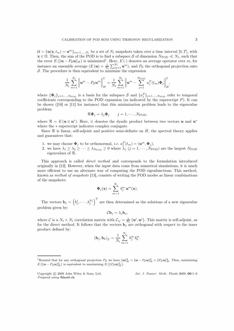
errors and costs vary extremely rapidly when α tends to 1, we have made the same choice asin [3], and introduced also a variation of these variables according to a parameter δ defined inincreasing bijection with α on [0, 1]. The weighting parameter α is defined by:

α =δ

ζ(i) (1 − δ) + δwith ζ(i) =

I(i)(yGP )

I(i)(0),

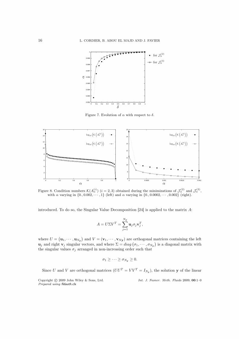
and is displayed as a function of δ in Fig. 7, with δ ∈ 0.05, 0.1, · · · , 1. The results computedwith a linear variation of δ on [0, 1] are represented in Fig. 6 (bottom). Numerically, whenα tends to 0, the trend tends towards a decrease of the normalized error (better calibratedmodel), and towards an increase of the cost of calibration (model more modified). In practice,it is thus difficult to exploit these curves to choose the value of the appropriate weightingparameter α. Of course, it is always possible to arbitrarily choose a criterion, ensuring aspecific balance between the reduction of the normalized error and the cost of calibration.However, as it has already been discussed in the previous section, the cost of the calibrationmeasured by the criterion D is not fully relevant. Then, we may wonder if it would not be moreconvenient to simply minimize the normalized error by setting α = 0. The answer is given in

Fig. 8, by showing that matrices A(2)α and A

(3)α become very ill-conditioned as α goes to 0. The

suggestion of [3] to add the term of calibration cost D to the functional can be interpreted asa particular method of regularization of the matrix A(i), which is, by nature, ill-conditioned.Moreover, the drawback of the procedure is the choice of the weighting parameter α which

is not straightforward. In addition, minimizing J (2)α and J (3)

α is impossible when coefficientsresulting from Galerkin projection are not available (case of the majority of the experimentaldata). In the next section, we thus propose another method of regularization directly basedon the minimization of I(3).

5. CALIBRATION BY TIKHONOV REGULARIZATION

5.1. Filter factors and discrete Picard condition

The minimization of the functional I(3) amounts to solving the linear system A(3)y = b(3)

where A(3) and b(3) are given in Appendix III. For the sake of clarity, the superscript isomitted and we thus write simply the linear system as Ay = b. In practice, the right-handside is contaminated by approximation errors related to the numerical evaluation of the time-derivatives of the POD eigenfunctions (remind that e(3)(0, t) = aP (t)). To understand theinfluence of these errors on the solution of the linear system, the concept of filter factors is



0.992

0.993

0.994

0.995

0.996

0.997

0.998

0.999

1

0 0.1 0.2 0.3 0.4 0.5 0.6 0.7 0.8 0.9 1

α

δ

for J (2)α

for J (3)α

Figure 7. Evolution of α with respect to δ.

0

2

4

6

8

10

12

14

16

0 0.2 0.4 0.6 0.8 1

α

log10

(

K(

A(2)α

))

log10

(

K(

A(3)α

))

8

9

10

11

12

13

14

15

0 0.0005 0.001 0.0015 0.002

α

log10

(

K(

A(2)α

))

log10

(

K(

A(3)α

))

Figure 8. Condition numbers K(A(i)α ) (i = 2, 3) obtained during the minimizations of J (2)

α and J (3)α ,

with α varying in 0., 0.002, · · · , 1 (left) and α varying in 0., 0.0002, · · · , 0.002 (right).

introduced. To do so, the Singular Value Decomposition [24] is applied to the matrix A:

A = UΣV T =

Ny∑

j=1

ujσjvTj ,

where U =(u1, · · · ,uNy

)and V = (v1, · · · ,vNy) are orthogonal matrices containing the left

uj and right vj singular vectors, and where Σ = diag(σ1, · · · , σNy

)is a diagonal matrix with

the singular values σj arranged in non-increasing order such that

σ1 ≥ · · · ≥ σNy≥ 0.

Since U and V are orthogonal matrices (UUT = V V T = INy), the solution y of the linear



Figure 9. Visual check of the discrete Picard condition corresponding to the minimization of I(3) withdetermination of all the coefficients (constant, linear and quadratic) and application of the Tikhonov

regularization (L = I ; y0 = yGP ).

system is given by‡:

y =

Ny∑

j=1

1

σj

uTj bvj =

Ny∑

j=1

hj

1

σj

uTj bvj with hj = 1 for j = 1, · · · , Ny,

where hj are the filter factors. This relation clearly illustrates the numerical difficultiesencountered when the linear system is solved without precautions. Indeed, if the Fouriercoefficients |uT

j b|, corresponding to the smaller singular values σj , do not decrease sufficientlyfast compared to the singular values, the solution is dominated by the terms in the sumcorresponding to the smallest σj . This behavior can be assessed by inspecting the discretePicard condition plotted in Fig. 9: for j ≃ 80, the singular values decay faster than the Fouriercoefficients |uT

j b|. As a result, the solution obtained presents many oscillations around zero,and thus appears to be completely random (see Fig. 10 for the solution without regularization).To fix this, the first idea is to modify the filter factor hj so that it behaves like an ideal low-pass

‡It can be shown easily (see Appendix III) that y is also the solution of the linear least-squares problem

miny ‖Ay − b‖22.



0 20 40 60 80 100 120 140 160 180−40

−30

−20

−10

0

10

20

30

40

50

No regularizationWith regularization

Figure 10. Comparison between solutions obtained with and without regularization, for theminimization of I(3), with the determination of all the coefficients (constant, linear and quadratic).The linear system is regularized by Tikhonov with L = I and y0 = yGP . Note that for Ngal = 6,

Ny = 168.

filter:

hj =

1 if j ≤ 80,

0 if j > 80.

For the cylinder wake flow, this procedure may be appropriate since the temporal dynamicsis relatively simple (see the abrupt falling-off in the singular values for j ≃ 80). However, thismethod is not suitable for more complex dynamics (3-D turbulent flow for instance) for whichthe singular values decrease continuously. It is thus necessary to modify the filter factors in amore sophisticated way.

5.2. Tikhonov regularization

Undoubtedly, the most common and well-known method of regularization is the Tikhonovregularization [25]. The idea is to seek the regularized solution yρ as the minimizer of thefollowing weighted functional

Φρ(y) = ‖Ay − b‖22 + ρ‖L (y − y0) ‖2

2,

where the first term corresponds to the residual norm, and the second to a side constraintimposed on the solution. ρ is called the regularization parameter and L represents the discreteapproximation matrix of a differential operator. This matrix is typically either the identity



matrix of order Ny (derivative of order zero), or a banded matrix of dimension (Ny − d)×Ny

approximation of the derivative operator of order d. In particular, for d = 0, d = 1 and d = 2,the method is termed zeroth, first and second-order Tikhonov regularization respectively.Thereafter, these operators will be denoted L = I (d = 0), L = FOD (d = 1) and L = SOD(d = 2).

Intuitively, the regularization can be seen as a balance between two requirements:

1. yρ should give a small residual Ayρ − b,2. L (yρ − y0) should be small with respect to the 2-norm.

10−8

10−6

10−4

10−2

100

102

10−2

10−1

100

101

102

20

406080100120140

160

180

200

residual norm ‖A(3)yρ − b(3)‖2

solu

tion

norm

‖Ly

ρ‖ 2

Figure 11. L-curve corresponding to the minimization of I(3), with the determination of all thecoefficients (constant, linear and quadratic) and application of the Tikhonov regularization (L = I ;

y0 = yGP ). The "corner" of the L-curve is at ρ = 6.78 10−8.

By using the same type of argument that that of section 5.1 to justify the introduction offilter factors hj , it becomes possible to prove that for y0 = 0, the regularized solution yρ canbe written as follows:

yρ =

Ny∑

j=1

hj

1

σj

uTj bvj with hj =

σ2j

σ2j + ρ

if L = INy,

and

yρ =

Ny−d∑

j=1

hj

1

σj

uTj bxj +

Ny∑

j=Ny−d+1

uTj bxj with hj =

γ2j

γ2j + ρ

if L 6= INy.



Here γj (j = 1, · · · , Ny − d) are the generalized singular values of (A, L) and xj the jthcolumn of X ∈ R

Ny×Ny (see Appendix V for the definition of the Generalized Singular ValueDecomposition).

The regularization parameter ρ needs now to be computed. To do so, the L-curve methodimplemented in the package Regularization Tools [26] is used throughout the paper.The L-curve method is based on the analysis of the curve representing the semi-norm ofthe regularized solution ‖Lyρ‖2, versus the corresponding residual norm ‖Ayρ −b‖2. In mostof the cases, this curve exhibits a typical L shape (see Fig. 11). The corner of the L-curverepresents a fair compromise between the minimization of the norm of the residual (horizontalbranch) and the semi-norm of the solution (vertical branch). In [26], the detection of the corneris based on the maximization of the curvature of the L-curve.

t

a1

0

0

1

1

2

2

3

3

4

4

5 6

−1

−2

−3

(a) Mode 1t

a3

0

0

1 2 3 4 5 6

0.1

0.2

0.3

0.4

0.5

−0.1

−0.2

−0.3

−0.4

−0.5

(b) Mode 3t

a6

0

0

1 2 3 4 5 6

0.1

0.2

0.3

0.4

0.5

−0.1

−0.2

−0.3

−0.4

(c) Mode 6


(POD ROM) mode amplitudes. The POD ROM is calibrated by minimizing I(3), with thedetermination of all the coefficients (constant, linear and quadratic). The linear system is regularized

by Tikhonov with L = I and y0 = yGP .

5.3. Comparison of the different types of Tikhonov regularization

Table II. Normalized errors E (i) and costs of the calibration D. Comparison between the resultsobtained by minimizing I(3), with the determination of all the coefficients (constant, linear andquadratic), for different types of Tikhonov regularization. The case L = FOD is not reported because

the numerical integration of the calibrated model is diverging.

Type of Tikhonov regularization√E (1)(y)

√

E (2)(y)√

E (3)(y)√

D(y)

L = I ; y0 = 0 4.14 10−3 2.33 10−1 6.27 10−2 8.90 10−1

L = I ; y0 = yGP 2.33 10−3 2.33 10−1 6.31 10−2 5.67 10−1

L = SOD ; y0 = 0 2.27 10−1 2.28 10−1 1.14 10−1 1.22L = SOD ; y0 = yGP 5.21 10−3 2.32 10−1 7.07 10−2 3.44 10−2

In this section, the various types of Tikhonov regularization introduced in section 5.2 arecompared on the configuration of the cylinder wake flow. Table II reports the normalized errors



0.01

0.1

1

10

1 2 3 4 5 6

POD index number i

Ener

get

icco

nte

nt

No calibration

Calibration

POD eigenvalues

Figure 13. Comparison between the modal energetic contents obtained before and after calibration.The POD eigenvalues are reported for reference. The POD ROM is calibrated by minimizing I(3),with the determination of all the coefficients (constant, linear and quadratic). The linear system is

regularized by Tikhonov with L = I and y0 = yGP .

and costs of the calibration obtained by zeroth and second-order Tikhonov regularization. Thecase of first-order Tikhonov regularization (L = FOD) is not mentioned because it is diverging,despite the regularization carried out. On average over all the criteria of normalized errors,the case L = I and y0 = yGP appears to be the most effective. Consequently, this type ofTikhonov regularization is retained for the comparison of section 5.4. In Fig. 12, the temporalevolutions of the POD modes are compared with those predicted by the calibrated reduced-order model. Contrary to the results presented in Fig. 4 there is no clear difference in thedynamics. The immediate consequence is that the modal energy distribution associated to thecalibrated model now corresponds perfectly to the POD energy (see figure 13). However, it isworth mentioning that the finite-time thermodynamics (FTT) formalism recently suggestedin [27] is more satisfactory because the calibration techniques are rather a posteriori methodswhereas the FTT is a flow modeling approach in itself.

5.4. Comparison of the most effective calibration methods

To conclude, we compare in this section the three most effective methods of calibrationpresented in this paper on the configuration of the wake flow. Table III gives the normalizederrors and the costs of the calibration obtained by minimization of I(1) under the constraint of

PC , by minimization of J (3)α for α = 0.001 and by minimization of I(3) with determination of

all the coefficients of the model and application of the most effective Tikhonov regularizationi.e. L = I and y0 = yGP . Except for the E(3) criterion where

√

E(3)(y) = 6.29 10−2 for the



minimization of J (3)α and

√

E(3)(y) = 6.31 10−2 for the minimization of I(3) with Tikhonovregularization, the numerical experiments prove that the normalized errors are minimized bythe calibration based on Tikhonov regularization. The difference between these methods of

calibration can be analyzed in a finer way by introducing the modal errors I(j)i defined§ for

i = 1, · · · , Ngal and j = 1, · · · , 3 as:

I(j) (y) =

Ngal∑

i=1

I(j)i (y) .

The modal errors I(1)i are represented in Fig. 14 for the various calibration techniques

presented in Table III. For all POD modes, the minimization of I(3) using the Tikhonov

regularization is more effective than the minimization of J (3)α for α = 0.001. Additionally,

these methods clearly outperform the minimization of I(1) under the constraint of PC for thehigher POD modes. The main interest of the calibration technique based on the Tikhonovregularization is that the choice of the parameter of regularization ρ is determined by theL-curve without any intervention of the user.

Table III. Normalized errors E (i) and costs of the calibration D. Comparison between the results

obtained by: i) minimizing I(1) under the constraint of PC , ii) minimizing J (3)α with α = 0.001, and

iii) minimizing I(3) with the determination of all the coefficients (constant, linear and quadratic) andapplication of the Tikhonov regularization (L = I ; y0 = yGP ).

Method of calibration Control terms√E (1)(y)

√

E (2)(y)√

E (3)(y)√

D(y)



Minimization of J (3)α (α = 0.001) C, L and Q 3.01 10−3 2.33 10−1 6.29 10−2 5.05 10−1

Minimization of I(3) with Tikhonov C, L and Q 2.33 10−3 2.33 10−1 6.31 10−2 5.67 10−1

regularization (L = I ; y0 = yGP )

6. CONCLUSIONS AND OUTLOOK

In the first part of this paper, we have presented within a unified framework the variousmethods of calibration used so far in the literature to identify the coefficients of the PODROM. Afterwards, we have applied these methods to a 2-D cylinder wake flow, to understandthese techniques in details, and, if possible, to release a more effective strategy. We have thusshowed that the minimization of I(1), under the constraint of the Cauchy problem PC , ismuch more effective than the methods based on the minimization of I(3), or than the IntrinsicStabilization scheme. We have then continued by applying the procedure suggested in [3],

§Rigorously, these modal errors can be introduced only when Λ is the identity matrix of size Ngal.



1e-008

1e-007

1e-006

1e-005

0.0001

0.001

0.01

1 2 3 4 5 6

POD mode i

I(1)

i

No calibration

Min. of I(1)


Min. of J (3)α (α = 0.001)

Min. of I(3) with Tikhonovregularization (L = I ; y0 = yGP )

Figure 14. Modal errors I(1)i . Comparison between the results obtained by: i) minimization of I(1)

under the constraint of PC , ii) minimization of J (3)α with α = 0.001 and iii) minimization of I(3) with

determination of all the coefficients (constant, linear and quadratic) and application of the Tikhonov

regularization (L = I ; y0 = yGP ). We remind that I(1) (y) =∑Ngal

i=1 I(1)i (y).

which is based on the minimization of a weighted sum of the normalized error, and of a termmeasuring the variation of the coefficients of the model to their values obtained by PODGalerkin. In substance, the idea is identical to what is usually made in optimal control ([28]for instance). Indeed, the cost functional is built as the sum of two terms, the first being ameasure of the objective of the optimization, and the second corresponding to the cost of thecontrol. However, as far as the identification is concerned, the variation of the coefficients ofthe calibrated model from their values obtained by POD Galerkin, is not relevant because themain objective is to improve the accuracy of the model. Also, in the case of experimental data,the coefficients resulting from POD Galerkin do not even exist in the majority of the cases.Finally, it can be shown numerically that adding the cost of the calibration to the functionalto be minimized, comes down to improve the conditioning of the linear systems associatedto the minimization of I(2) and I(3). As the choice of the parameter α is relatively tricky,even arbitrary, the linear system associated to the minimization of I(3) is regularized by themethod of Tikhonov. For our test-case, the zeroth-order regularization (L = I) with y0 = yGP

is the most effective among all the types of Tikhonov regularization considered. Lastly, ournumerical experiments demonstrate that the Tikhonov regularization outperforms, in terms ofnormalized errors, the minimization of I(1) under the constraint of PC and the minimization of

J (3)α with α = 0.001. Compared to the approach suggested in [3], the interest of the Tikhonov

regularization is that the value of the parameter of regularization ρ is determined automatically,via the L-curve method.



The calibration by Tikhonov regularization presented here still needs to be tested onflow configurations corresponding to more complex dynamics: 3-D turbulent flow obtainedby numerical simulations, and challenging experimental data. The extension to actuatedconfigurations with known control parameters should be straightforward. On the other hand,calibrating a reduced-order model, so that it can represent the evolution of dynamics when thecontrol law varies, is a more complex task. A basic idea consists in determining a POD basisstarting from snapshots coming from several control laws, and then to calibrate the model forall the control laws considered. Recently, this approach was applied for the first time in [1] toidentify a robust model of actuated wakes.

APPENDIX

I. POD ROM COEFFICIENTS

The coefficients of the POD ROM (3) obtained by Galerkin projection (GP) are:

AGPi = − (Φi, (um · ∇)um)Ω − 1

Re

((∇⊗ Φi)

T , ∇⊗ um

)

Ω+

1

Re[(∇⊗ um)Φi]∂Ω ,

BGPij = − (Φi, (um · ∇)Φj)Ω − (Φi, (Φj · ∇)um)Ω − 1

Re

((∇⊗ Φi)

T , ∇⊗ Φj

)

Ω

+1

Re[(∇⊗ Φj)Φi]∂Ω ,

CGPijk = − (Φi, (Φj · ∇)Φk)Ω ,

DGPi = − (Φi, uc)Ω ,

EGPi = − (Φi, (uc · ∇)um)Ω − (Φi, (um · ∇)uc)Ω − 1

Re

((∇⊗ Φi)

T , ∇⊗ uc

)

Ω

+1

Re[(∇⊗ uc)Φi]∂Ω ,

FGPij = − (Φi, (Φj · ∇)uc)Ω − (Φi, (uc · ∇)Φj)Ω ,

GGPi = − (Φi, (uc · ∇)uc)Ω ,

with [u]∂Ω =

∫

∂Ω

u · n dx and(

P , Q)

Ω=

∫

Ω

P : Qdx =

nc∑

i, j=1

∫

Ω

PijQji dx. Here,

nc is the number of components of u. When the flow is not controlled, uc = 0 and



DGPi = EGP

i = FGPij = GGP

i = 0. When U = uii=1,...,Nt, we have um = 0 and AGP

i = 0.

II. EVALUATION OF f AND g

The values of fi and gi (see section 2.2.2 for their definitions) can be easily determined if weknow the coefficients yi and zi. Indeed, fi belongs to the space of polynomials of degree 2 inNgal variables: aR

1 (t), · · · , aRNgal

(t). Therefore, let

m(t) =

1aR1 (t)...

aRNgal

(t)

aR1 (t)aR

1 (t)...

aRNgal

(t)aRNgal

(t)

∈ RNyi

be the vector containing the natural monomial basis of this space, we can write:

fi(yi,aR(t)) = m(t) · yi.

Similarly, if we define

q(t) =

γ(t)γ(t)

γ(t)aR1 (t)

...γ(t)aR

Ngal(t)

γ2(t)

∈ RNzi ,

we have:gi(zi,a

R(t), γ) = q(t) · zi.

We can deduce from these expressions that f can be computed at any time instant t, asthe product of a block diagonal matrix M where each block is equal to mT by the vector y.Similarly, g can be obtained as the product of a block diagonal matrix Q where each block isgiven by qT by the vector z.

III. MINIMIZATION OF I(2) AND I(3)

For i = 2 and 3, e(i) is an affine function with respect to y ∈ RNy (see sections 3.1.2 and

3.1.3). Therefore, we introduce the application

e(i)(·, t) :RNy → RNgal

y 7→ E(i)(t)y + e(i)(0, t) with E(i)(t) ∈ RNgal×Ny .

By identification with the expressions of the errors e(i) (i = 1, 2), one finds immediatelythat:



• for i = 2

E(2)(t)y = −∫ t

0

f(y,aP (τ)) dτ and e(2)(0, t) = aP (t) − aP (0)

• for i = 3

E(3)(t)y = −f(y,aP (t)) and e(3)(0, t) = aP (t),

where f can be evaluated using the method described in Appendix II.

Assuming that Λ is symmetric, we can prove that for i = 2 and 3:

I(i)(y) = 〈‖e(i)(y, t)‖2Λ〉To

= yT 〈E(i)(t)T ΛE(i)(t)〉Toy + 2 〈e(i)(0, t)T ΛE(i)(t)〉To

y

+ 〈e(i)(0, t)T Λe(i)(0, t)〉To,

= yT A(i)y − 2b(i)Ty + c(i),

where

A(i) = 〈E(i)T (t)ΛE(i)(t)〉To∈ R

Ny×Ny ,

b(i) = −〈E(i)T (t)Λe(i)(0, t)〉To∈ R

Ny ,

c(i) = 〈e(i)(0, t)T Λe(i)(0, t)〉To∈ R.

If Λ is a symmetric matrix, then A(i) is also symmetric by construction. In that case,minimizing the quadratic function I(i) is equivalent to solve the linear system defined by:

A(i)y = b(i).

IV. MINIMIZATION OF J (i)α

The functional J (i)α can also be written as:

J (i)α (y) = χα

A I(i)(y)︸︷︷︸

f1(y)

+χαΠ ‖y − yGP ‖2

Π︸︷︷︸

f2(y)

,

by denoting

χαA =

1 − α

I(i)(yGP )and χα

Π =α

‖yGP ‖2Π

.

In Appendix III, we have demonstrated that when Λ is a symmetric matrix we have

f1(y) = yT A(i)y−2b(i)T y+c(i). Similarly, it can be shown that f2(y) = yT Πy−2yGP TΠy+

yGP TΠyGP if we assume that Π is symmetric.

Since f1 and f2 are two quadratic functions, it is simple to evaluate their gradients at y.One obtains:

∇f1 (y) = 2(

A(i)y − b(i))

and ∇f2 (y) = 2Π(y − yGP

).



By definition, the functional J (i)α is minimal at y

(i)α when ∇J (i)

α

(

y(i)α

)

= 0. Minimizing

J (i)α (y) for i = 2 or 3 is then equivalent to solve the linear system:

A(i)α y(i)

α = b(i)α ,

withA(i)

α = χαA A(i) + χα

Π Π,

andb(i)

α = χαA b(i) + χα

Π ΠyGP .

Note that for α = 0, χαA = 1

I(i)(yGP )and χα

Π = 0. Inserting these relations into (7), the linear

system (6) is recovered.

V. GENERALIZED SINGULAR VALUE DECOMPOSITION

Let A ∈ Rm×n and L ∈ R

p×n be given with m ≥ n ≥ p. There exist orthogonal matricesU ∈ R

m×n and V ∈ Rp×p and a nonsingular matrix X ∈ R

n×n such that

A = U

(Σ 00 In−p

)

X−1 , L = V (M, 0)X−1

where Σ = diag(σ1, · · · , σp) and M = diag(µ1, · · · , µp) with 0 ≤ σ1 ≤ · · · ≤ σp ≤ 1 and1 ≥ µ1 ≥ · · · ≥ µp ≥ 0. Furthermore, it holds that σ2

j + µ2j = 1 for j = 1, · · · , p. The values

γj = σj/µj (j = 1, · · · , p) are called the generalized singular values of (A, L). The jth columnxj of X is the right singular vector associated with σj .



ACKNOWLEDGEMENTS

A preliminary version of this work was presented at the workshop on "Industrial applications of loworder models based on POD" organized by Angelo Iollo (IMB - Bordeaux University and MC2 -INRIA Bordeaux Sud-Ouest). This workshop held at Bordeaux on March 31 - April 2, 2008 was verystimulating and nevertheless friendly. LC is very indebted to Angelo for inviting him to give a talk. Theextension of the Tikhonov regularization method to the first and second order presented in this paperwas suggested by I. M. Navon (School of Computational Science and Department of Mathematics,Florida State University) during the workshop. LC is very grateful to him for this suggestion. Lastbut not least, LC would like to acknowledge Bernd R. Noack and the low-dimensional modelingand control team at the Technische Universität Berlin for stimulating and fruitful discussions.

REFERENCES

1. Weller J, Lombardi E, Iollo A. Robust model identification of actuated vortex wakes. Physica D: NonlinearPhenomena 2009; 238:416–427.

2. Galletti B, Bruneau CH, Zannetti L, Iollo A. Low-order modelling of laminar flow regimes past a confinedsquare cylinder. J. Fluid Mech. 2004; 503:161–170.

3. Couplet M, Basdevant C, Sagaut P. Calibrated Reduced-Order POD-Galerkin system for fluid flowmodelling. J. Comp. Phys. 2005; 207:192–220.

4. Bergmann M, Cordier L, Brancher JP. Optimal rotary control of the cylinder wake using POD ReducedOrder Model. Phys. Fluids 2005; 17(9):097 101:1–21.

5. Perret L, Collin E, Delville J. Polynomial identification of POD based low-order dynamical system. Journalof Turbulence 2006; 7:1–15.

6. Galletti B, Bottaro A, Bruneau CH, Iollo A. Accurate model reduction of transient and forced wakes. Eur.J. Mech. B/Fluids 2007; 26(3):354–366.

7. Kalb VL, Deane AE. An intrinsic stabilization scheme for proper orthogonal decomposition based low-dimensional models. Phys. Fluids 2007; 19:054 106.

8. Tikhonov AN, Arsenin VY. Solutions of ill posed problems. Winston and Sons, 1977.9. Alekseev AK, Navon IM. The Analysis of an Ill-Posed Problem Using Multiscale Resolution and Second

Order Adjoint Techniques. Computer Methods in Applied Mechanics and Engineering 2001; 190(15-17):1937–1953.

10. Rowley CW. Modeling, simulation and control of cavity flow oscillations. Phd thesis, California Instituteof Technology 2002.

11. Cordier L, Bergmann M. Proper Orthogonal Decomposition: an overview. Lecture series 2002-04, 2003-03 and 2008-01 on post-processing of experimental and numerical data. Von Kármán Institute for FluidDynamics, 2008.

12. Lumley JL. Atmospheric Turbulence and Wave Propagation. The structure of inhomogeneous turbulence.Nauka, Moscow, 1967; 166–178.

13. Sirovich L. Turbulence and the dynamics of coherent structures. Quarterly of Applied Mathematics 1987;XLV(3):561–590.

14. Noack BR, Afanasiev K, Morzyński M, Tadmor G, Thiele F. A hierarchy of low-dimensional models forthe transient and post-transient cylinder wake. J. Fluid Mech. 2003; 497:335–363.

15. Cordier L, Bergmann M. Two typical applications of POD: coherent structures eduction and reduced ordermodelling. Lecture series 2002-04, 2003-03 and 2008-01 on post-processing of experimental and numericaldata. Von Kármán Institute for Fluid Dynamics, 2008.

16. Bergmann M, Cordier L. Optimal control of the cylinder wake in the laminar regime by Trust-Regionmethods and POD Reduced Order Models. J. Comp. Phys. 2008; 227:7813–7840.

17. Bergmann M, Cordier L. Control of the circular cylinder wake by Trust-Regionmethods and POD Reduced-Order Models. Research Report 6552, INRIA 06 2008. URLhttps://hal.inria.fr/inria-00284258.



18. Noack BR, Cordier L, Morzyński M, Tadmor G. Reduced Order Models for Analysis and Control of FluidFlows. Technical Report, Hermann-Föttinger-Institut für Ströungsmechanik, Technische Universität Berlin2005.

19. Favier J. Contrôle d’écoulements : approche expérimentale et modélisation de dimension réduite. Phdthesis, Institut National Polytechnique de Toulouse, France 2007.

20. Iollo A, Lanteri S, Désidéri JA. Stability properties of POD-Galerkin approximations for the compressibleNavier-Stokes equations. Technical Report 3589, INRIA 1998.

21. Rempfer D. On low-dimensional Galerkin models for fluid flow. Theor. Comput. Fluid Dyn. 2000; 14:75–88.22. Bergmann M. Optimisation aérodynamique par réduction de modèle POD et contrôle optimal. Application

au sillage laminaire d’un cylindre circulaire. Phd thesis, Institut National Polytechnique de Lorraine,Nancy, France 2004.

23. Bourguet R, Braza M, Dervieux A. Reduced-order modeling for unsteady transonic flows around an airfoil.Phys. Fluids 2007; 19(11):111 701:1–4.

24. Golub GH, Van Loan CF. Matrix Computations. 3 edn., The Johns Hopkins University Press: Baltimoreand London, 1996.

25. Hansen PC. Rank-Deficient and Discrete Ill-Posed Problems: Numerical Aspects of Linear Inversion.SIAM, Philadelphia, 1998.

26. Hansen PC. Regularization Tools: A Matlab package for analysis and solution of discrete ill-posedproblems. Numerical Algorithms 1994; 6:1–35.

27. Noack BR, Schlegel M, Ahlborn B, Mutschke G, Morzyński M, Comte P, Tadmor G. A finite-timethermodynamics formalism for unsteady flows. J. Non-Equilib. Thermodyn. 2008; 33(2):103–148.

28. Gunzburger MD. Introduction into mathematical aspects of flow control and optimization. Lecture series1997-05 on inverse design and optimization methods. Von Kármán Institute for Fluid Dynamics, 1997.

Contents

1 INTRODUCTION 1

2 REDUCED-ORDER MODELING BASED ON A POD GALERKIN AP-

PROACH 2

2.1 Proper Orthogonal Decomposition . . . . . . . . . . . . . . . . . . . . . . . . . . . . . 22.2 POD Reduced-Order Model based on Galerkin projection . . . . . . . . . . . . . . . . 4

2.2.1 General description . . . . . . . . . . . . . . . . . . . . . . . . . . . . . . . . . . 42.2.2 Simplification of the POD ROM . . . . . . . . . . . . . . . . . . . . . . . . . . 5

2.3 Two-dimensional cylinder wake flow at Re = 200 . . . . . . . . . . . . . . . . . . . . . 6

3 EXISTING CALIBRATION METHODS 8

3.1 Definitions of errors . . . . . . . . . . . . . . . . . . . . . . . . . . . . . . . . . . . . . 93.1.1 State calibration method with dynamical constraints . . . . . . . . . . . . . . . 93.1.2 State calibration method . . . . . . . . . . . . . . . . . . . . . . . . . . . . . . 103.1.3 Flow calibration method . . . . . . . . . . . . . . . . . . . . . . . . . . . . . . . 11

3.2 Affine functions of errors . . . . . . . . . . . . . . . . . . . . . . . . . . . . . . . . . . . 113.3 Calibration procedure proposed in [3] . . . . . . . . . . . . . . . . . . . . . . . . . . . . 11

4 APPLICATION TO THE CYLINDER WAKE FLOW 13

4.1 Minimization of I(1) under the constraint of PC and minimization of I(3) . . . . . . . 13

4.2 Minimizations of J (2)α and J (3)

α . . . . . . . . . . . . . . . . . . . . . . . . . . . . . . . 14

5 CALIBRATION BY TIKHONOV REGULARIZATION 15

5.1 Filter factors and discrete Picard condition . . . . . . . . . . . . . . . . . . . . . . . . 155.2 Tikhonov regularization . . . . . . . . . . . . . . . . . . . . . . . . . . . . . . . . . . . 185.3 Comparison of the different types of Tikhonov regularization . . . . . . . . . . . . . . 205.4 Comparison of the most effective calibration methods . . . . . . . . . . . . . . . . . . 21

6 CONCLUSIONS AND OUTLOOK 22



I POD ROM COEFFICIENTS 24

II EVALUATION OF f AND g 25

IIIMINIMIZATION OF I(2)AND I(3)

25

IV MINIMIZATION OF J (i)α 26

V GENERALIZED SINGULAR VALUE DECOMPOSITION 27


calibration of pod reduced-order models using tikhonov

Documents