CALL CENTER OUTSOURCING CONTRACT DESIGN

AND CHOICE

O. Zeynep Aksin∗

Francis de Vericourt†

Fikri Karaesmen‡

∗ College of Administrative Sciences and Economics

Koc University

34450, Sariyer, Istanbul, TURKEY

zaksin@ku.edu.tr

† Fuqua School of Business

Duke University

Durham, NC, USA

fdv1@mail.duke.edu

‡ Department of Industrial Engineering

Koc University

34450, Sariyer, Istanbul, TURKEY

fkaraesmen@ku.edu.tr

Call Center Outsourcing Contract Design and Choice

O. Zeynep Aksin Francis de Vericourt Fikri Karaesmen

October 2004

Abstract

This paper considers a call center outsourcing contract design and choice problem, faced

by an outsourcing vendor and a service provider. The service provider receives an uncertain

call volume over multiple-periods, and is considering outsourcing all or part of these calls to

an outsourcing vendor. Each call brings in a fixed revenue to the service provider. Answering

calls requires having service capacity, thus implicit in the outsourcing decision is a capacity

decision. Insufficient capacity implies that calls cannot be answered, which in turn means

there will be a revenue loss. Faced with a choice between a volume-based and a capacity-

based contract offered by an outsourcing vendor who has pricing power, the service provider

determines optimal capacity levels. The optimal price and capacity of the outsourcing vendor

together with the optimal capacity of the service provider determine optimal profits of each

party under the two contracts being considered. Each party will prefer the contract that leads

to higher profits. The paper characterizes optimal capacity levels, and partially characterizes

optimal pricing decisions under each contract. The impact of demand variability and economic

parameters on contract choice are explored through numerical examples. It is shown that no

contract type is universally preferred, and that operating environments as well as cost-revenue

structures have an important effect in outsourcing contract design and choice.

Keywords: call center; outsourcing; contract design; contract choice; capacity investment;

exogeneous and endogeneous price.

1 Introduction

A growing number of companies outsource their call center operations. According to International

Data Corporation (1999), the worldwide call center services market totalled $ 23 billion in revenues

in 1998, and is estimated to double to $ 8.6 billion by 2003. Outsourcing constitutes 74 % of

this market and is projected to be $42 billion in 2003. Datamonitor (1999) expects call center

1

outsourcing to boom in Europe, where the $ 7 billion market in 1999 is expected to grow to $15

billion by 2004. In terms of outsourced agent positions, this constitutes a growth from 74,000 in

1999 to 126,500 in 2003.

While for some companies outsourcing the entire call center operation constitutes the best

option, many are hesitant to hand over their most important source of customer contact to another

firm. This has led to the emergence of the practice known as co-sourcing (Fuhrman, 1999), where

some calls are kept in-house while others are outsourced. The decision of how to share calls in a

co-sourcing setting is an important one. In practice, this can take many forms where for example

certain types of calls are outsourced and others are kept in-house, or overflow calls in all functions

are outsourced. Whatever the chosen form of sharing, detailed outsourcing contracts that specify

requirements, service levels, and price are deemed necessary for success (Lacity and Willcox, 2001).

This paper is motivated by the call center outsourcing problem of a major mobile telecommu-

nications service provider in Europe. The overall objective is to evaluate two types of contracts

made available to this company by an outsourcing vendor (contractor). In making this comparison,

detailed contracts that specify capacity (and implicitly service levels) and price within each type

of contract will be considered. Like in most call center outsourcing situations, the outsourcing

vendor operates a much larger call center operation compared to the one by the operator. This

allows the vendor to have an advantageous cost structure and power in negotiating prices. The

telecommunications service provider opted for a co-sourcing solution. Accordingly, some call types

would be kept in-house while others would be shared with an outsourcing vendor. This paper is

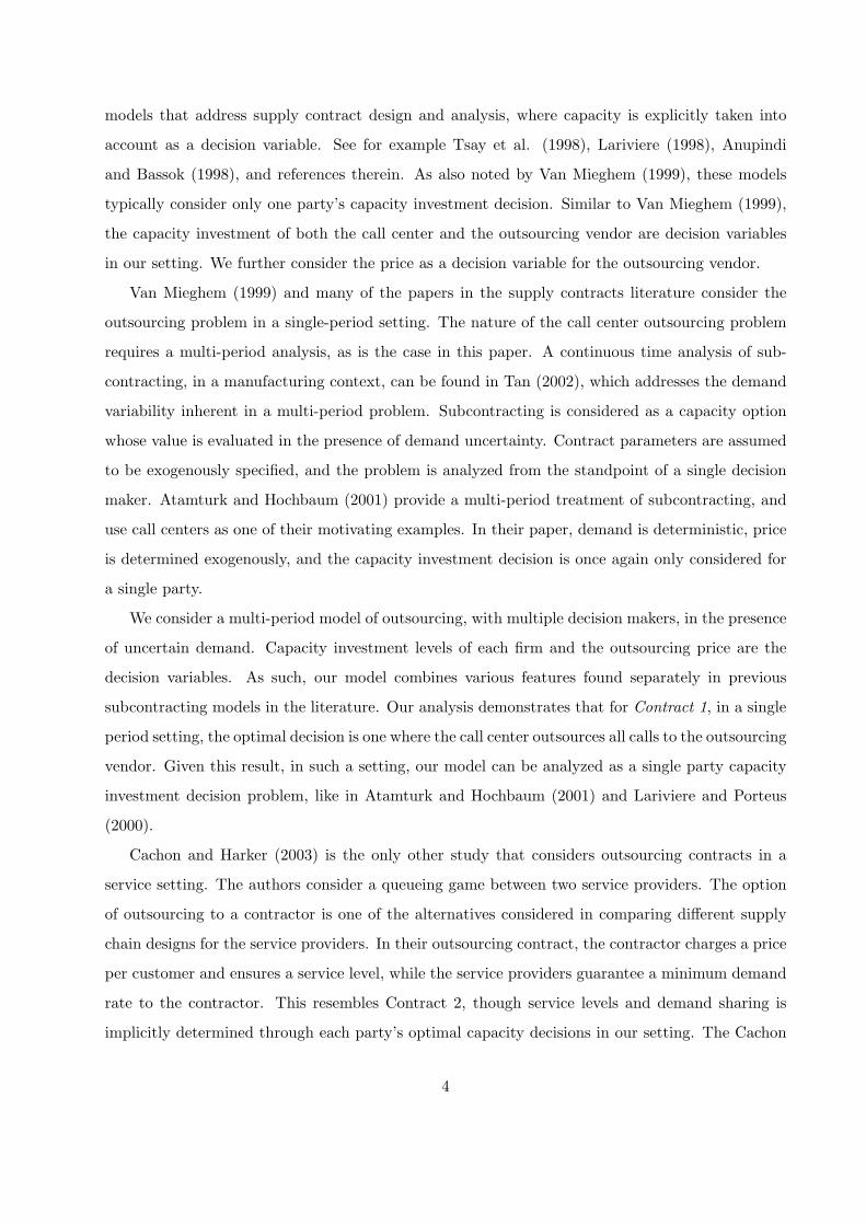
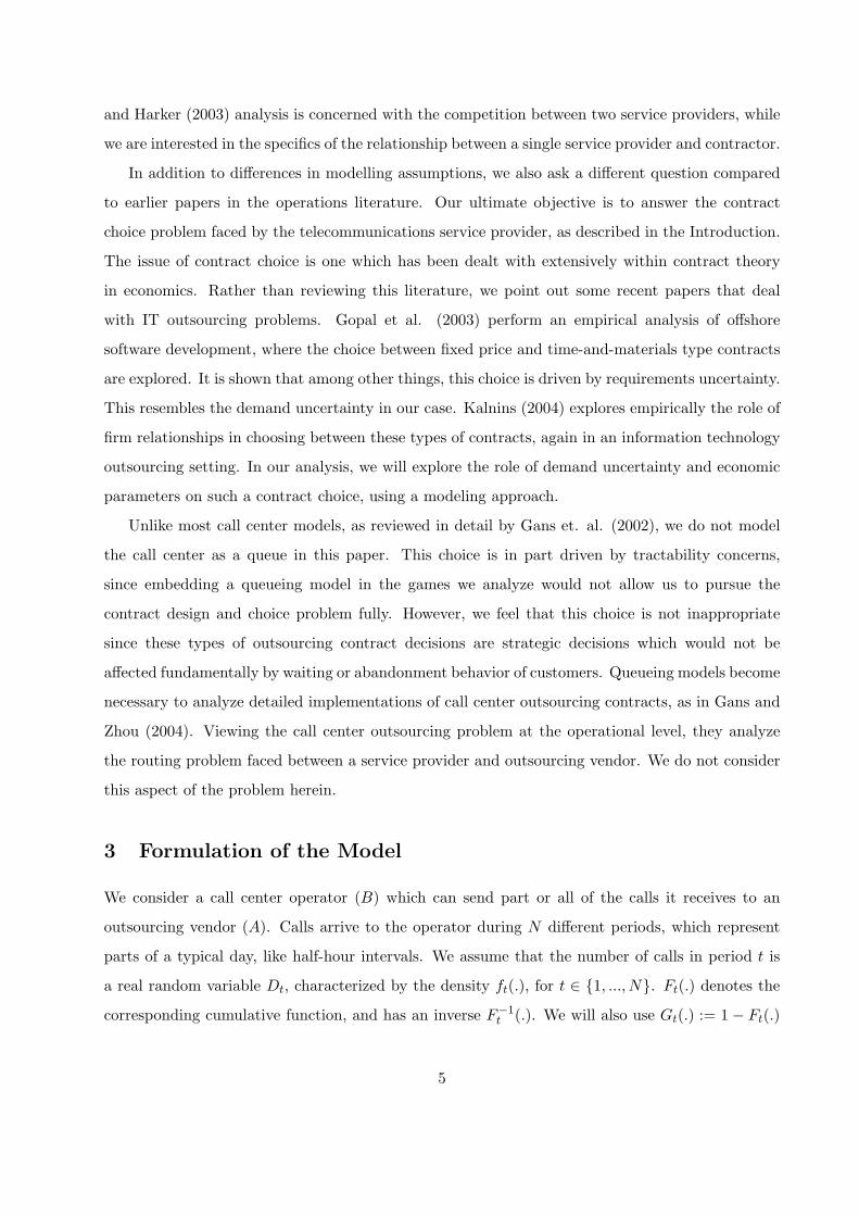
only concerned with the latter sharing of the calls. The vendor proposed two forms of sharing. The

first type, which we label as Contract 1 or as subcontracting the base, is a form of capacity reser-

vation whereby the company reserves enough capacity for a steady level of calls at the outsourcing

vendor for a given fee. All calls in excess of this level are considered for treatment in-house. The

second type of contract, labeled as Contract 2 or as subcontracting the fluctuation, stipulates that

the telecommunication service provider answers all calls up to a specified level in-house, beyond

which calls are diverted to the outsourcing vendor. In other words, in this type of contract overflow

calls are outsourced. The vendor charges a fee per call treated. These two cases are illustrated in

Figure 1. In both settings, the outsourcing vendor has pricing power. Both parties try to maximize

their own profits.

While we are motivated by this particular instance, we note that the problem is common to

call center outsourcing in general. As also noted by Gans and Zhou (2004), call center outsourcing

2

Contract 1: Subcontracting the base

calls

outsource

keep in house

t

outsource

keep in house

t

Contract 2: Subcontracting the fluctuation

calls

Figure 1: The two contracts offered by the outsourcing vendor

contracts are typically volume-based or capacity-based. The former type of contract implies a per-

call pricing as in our Contract 2 and the latter implies a per-agent-per-hour type of pricing which

resembles Contract 1. In order to model the contract choice problem, we specify these contracts in

more detail, using our motivating instance to do this.

For the service outsourcing problem, we analyze the optimal capacity and pricing decisions

under each contract type. We then explore the telecommunication service provider’s basic question,

namely which contract type they should prefer. Current practice at the company is to co-source

with a contract of the form subcontracting the base. While basic operations management intuition

would suggest that keeping the less variable portion of the demand in-house and outsourcing the

high variation overflow would be more beneficial, we illustrate that both contract types may be

preferred, depending on economic parameters and demand characteristics. In the following section,

we provide a brief literature review. Section 3 formulates the model. This is then analyzed in order

to determine optimal service capacities in Section 4 and the optimal prices in Section 5. Section

6 presents a numerical study to illustrate the relationships between contract parameters, demand

characteristics, and contract preferences of each party. We provide concluding remarks in Section

7.

2 Literature Review

The problem of outsourcing or subcontracting has been studied in the economics literature in the

context of vertical integration. This literature does not consider capacity constraints. Kamien et

al. (1989), Kamien and Li (1990) first model capacity constraints, either implicitly or explicitly,

in the context of subcontracting production. The supply chain literature provides a rich set of

3

models that address supply contract design and analysis, where capacity is explicitly taken into

account as a decision variable. See for example Tsay et al. (1998), Lariviere (1998), Anupindi

and Bassok (1998), and references therein. As also noted by Van Mieghem (1999), these models

typically consider only one party’s capacity investment decision. Similar to Van Mieghem (1999),

the capacity investment of both the call center and the outsourcing vendor are decision variables

in our setting. We further consider the price as a decision variable for the outsourcing vendor.

Van Mieghem (1999) and many of the papers in the supply contracts literature consider the

outsourcing problem in a single-period setting. The nature of the call center outsourcing problem

requires a multi-period analysis, as is the case in this paper. A continuous time analysis of sub-

contracting, in a manufacturing context, can be found in Tan (2002), which addresses the demand

variability inherent in a multi-period problem. Subcontracting is considered as a capacity option

whose value is evaluated in the presence of demand uncertainty. Contract parameters are assumed

to be exogenously specified, and the problem is analyzed from the standpoint of a single decision

maker. Atamturk and Hochbaum (2001) provide a multi-period treatment of subcontracting, and

use call centers as one of their motivating examples. In their paper, demand is deterministic, price

is determined exogenously, and the capacity investment decision is once again only considered for

a single party.

We consider a multi-period model of outsourcing, with multiple decision makers, in the presence

of uncertain demand. Capacity investment levels of each firm and the outsourcing price are the

decision variables. As such, our model combines various features found separately in previous

subcontracting models in the literature. Our analysis demonstrates that for Contract 1, in a single

period setting, the optimal decision is one where the call center outsources all calls to the outsourcing

vendor. Given this result, in such a setting, our model can be analyzed as a single party capacity

investment decision problem, like in Atamturk and Hochbaum (2001) and Lariviere and Porteus

(2000).

Cachon and Harker (2003) is the only other study that considers outsourcing contracts in a

service setting. The authors consider a queueing game between two service providers. The option

of outsourcing to a contractor is one of the alternatives considered in comparing different supply

chain designs for the service providers. In their outsourcing contract, the contractor charges a price

per customer and ensures a service level, while the service providers guarantee a minimum demand

rate to the contractor. This resembles Contract 2, though service levels and demand sharing is

implicitly determined through each party’s optimal capacity decisions in our setting. The Cachon

4

and Harker (2003) analysis is concerned with the competition between two service providers, while

we are interested in the specifics of the relationship between a single service provider and contractor.

In addition to differences in modelling assumptions, we also ask a different question compared

to earlier papers in the operations literature. Our ultimate objective is to answer the contract

choice problem faced by the telecommunications service provider, as described in the Introduction.

The issue of contract choice is one which has been dealt with extensively within contract theory

in economics. Rather than reviewing this literature, we point out some recent papers that deal

with IT outsourcing problems. Gopal et al. (2003) perform an empirical analysis of offshore

software development, where the choice between fixed price and time-and-materials type contracts

are explored. It is shown that among other things, this choice is driven by requirements uncertainty.

This resembles the demand uncertainty in our case. Kalnins (2004) explores empirically the role of

firm relationships in choosing between these types of contracts, again in an information technology

outsourcing setting. In our analysis, we will explore the role of demand uncertainty and economic

parameters on such a contract choice, using a modeling approach.

Unlike most call center models, as reviewed in detail by Gans et. al. (2002), we do not model

the call center as a queue in this paper. This choice is in part driven by tractability concerns,

since embedding a queueing model in the games we analyze would not allow us to pursue the

contract design and choice problem fully. However, we feel that this choice is not inappropriate

since these types of outsourcing contract decisions are strategic decisions which would not be

affected fundamentally by waiting or abandonment behavior of customers. Queueing models become

necessary to analyze detailed implementations of call center outsourcing contracts, as in Gans and

Zhou (2004). Viewing the call center outsourcing problem at the operational level, they analyze

the routing problem faced between a service provider and outsourcing vendor. We do not consider

this aspect of the problem herein.

3 Formulation of the Model

We consider a call center operator (B) which can send part or all of the calls it receives to an

outsourcing vendor (A). Calls arrive to the operator during N different periods, which represent

parts of a typical day, like half-hour intervals. We assume that the number of calls in period t is

a real random variable Dt, characterized by the density ft(.), for t ∈ {1, ..., N}. Ft(.) denotes the

corresponding cumulative function, and has an inverse F−1t (.). We will also use Gt(.) := 1− Ft(.)

5

and Gt(.) :=∑t

τ=1 Gτ (.), where t ∈ {0 . . . N} with G0(x) := −∞.

A contract specifies how the arriving calls are distributed between the operator and the con-

tractor. Calls that are not answered by either the operator or the contractor are lost. On the other

hand, an answered call brings a revenue of r per unit to the operator, even when that call was

handled by the contractor. In the following, we analyze two types of contracts.

The operator chooses a service capacity level KBt for each period t. Similarly KA

t denotes the

service capacity of the contractor for period t. We define cB and cA, the unit costs of the service

capacity level per period for the operator and the contractor respectively. It is assumed throughout

that cA < cB. In the first type of contract, all the KAt ’s, t ∈ {1, ..., N} are equal to a unique

capacity KA which is fixed by the operator, while in the second one, these levels are chosen by the

contractor. We denote by Kt := KA +KBt , the total service capacity of the system in Period t. All

parameters are common knowledge.

3.1 Contract 1: Subcontracting the Base

In this contract, the operator specifies the capacity level KA of the contractor. This capacity level

will remain constant during the day, namely KAt = KA for t ∈ {1, ..., n}. In turn, the contractor

charges a capacity reservation price γ per unit of capacity and per period. This contract is only

attractive to the operator if cB > γ. Otherwise the operator keeps all capacity in-house.

The operator chooses KA and KBt , t ∈ {1, ..., N} in order to maximize its total profit πB, which

is equal to,

πB =N∑

t=1

πBt (1)

where πBt is the profit for period t given by:

πBt = rE[min(Dt,Kt)]− cBKB

t − γKA. (2)

The corresponding total profit of the contractor is equal to,

πA = N(γ − cA)KA. (3)

For the time being γ can be regarded as an exogenously determined contract parameter. Section

5 focuses on the case where the contractor sets γ in order to maximize its profit πA.

6

3.2 Contract 2: Subcontracting the fluctuation

In this contract, the operator sends all calls it cannot answer to the contractor. The contractor

charges a unit price p per answered call. Calls that are not handled by the contractor do not incur

any payment. This contract will lead to the outsourcing of some calls by the operator only if r > p

since the firm has no interest to outsource calls otherwise.

Hence, in period t, the operator first tries to saturate his service capacity KBt , before send-

ing calls to the contractor. In other words, the number of calls DBt received by the operator is

equal to min(Dt,KBt ). The corresponding number DA

t received by the contractor is then equal to

max(0, Dt −KBt ).

The operator chooses KBt , t ∈ {1, ..., N} in order to maximize its total profit, which is equal

to,

πB =N∑

t=1

πBt (4)

where πBt is the given by:

πBt = rE[min(Dt,Kt)]− cBKB

t − pE[min(DAt ,KA

t )]. (5)

For this type of contract, the contractor chooses KAt , t ∈ {1, ..., N} in order to maximize its total

profit,

πA =N∑

t=1

πAt (6)

where πAt is given by:

πAt = pE[min(DA

t ,KAt )]− cAKA

t . (7)

Once again, as far as the capacity decisions are considered p can be viewed as an exogenously

determined parameter. Section 5 focuses on the more complicated pricing problem where the

contractor selects p in order to maximize πA.

4 Optimal Service Capacities

In this section, we derive the optimal service capacity levels for both contracts. For the time being,

we assume an exogenously set price γ or p.

4.1 Contract 1: Subcontracting the Base

The following theorem provides the optimal capacity levels that the operator should set.

7

Proposition 1 The capacity levels KA∗ and KB∗t , t ∈ {1, ....N}, which maximize the operator’s

profit function can be characterized as follows:

1. Determine φt for t ∈ {1, ....N}, where φt := F−1t (1− cB/r),

2. Re-index the periods such that φ1 ≤ ... ≤ φt ≤ ... ≤ φN ,

3. Compute κt := G−1t ( tcB−N(cB−γ)

r ) for t ∈ {1, ....N},

4. Define t∗ the time period such that, t∗ = max(t, t ∈ {1, ....N}; φt ≤ κt−1).

5. Compute KA∗ and KB∗t as follows,

KA∗ = max(κt∗ , φt∗)

KB∗t = max(0, φt −KA∗), for t ∈ {1, ....N}

Proof: Assume that the first four steps have been completed. The derivative of πB with respect

to KBt is equal to,

∂πB

∂KBt

= rGt(Kt)− cB (8)

and πB is concave with respect to KBt . It follows that ∂πB

∂KBt≥ 0 ⇔ Kt ≤ φt. Hence, if KA ≤ φt,

πB reaches its maximum for KBt = Φt − KA when all the other capacity levels are fixed. If

not, the profit function is strictly decreasing and its maximum is obtained when KBt = 0. In

short, KBt is equal to max(0, φt −KA). It remains to compute the value of KA which maximizes

πB(KA) := πB(KA, (max(0, φt −KA))t∈{1,....N}).

For a given period τ , consider values of KA in the interval [φτ , φτ+1]. For all t ≤ τ , KBt =

max(0, φt − KA) = 0 and Kt = KA. KBt and Kt are respectively equal to φt − KA and φt

otherwise. Hence the profit function is equal to:

πB(KA) =τ∑

t=1

(r

∫ KA

0xft(x)dx + (rGt(KA)− γ)KA

)

+N∑

τ+1

(r

∫ φt

0xft(x)dx + (rGt(φt)− γ − cB)φt

)

+(N − τ)(cB − γ)KA. (9)

This function is twice differentiable for φτ ≤ KA ≤ φτ+1, and we have for the first and second

order derivatives, (we assume in the rest of the proof that derivatives computed on the lower-bound

8

(resp. upper-bound) of an interval correspond to the right (resp. left) hand derivatives)

πB′(KA) = rGτ (KA)− γτ + (N − τ)(cB − γ) (10)

πB′′(KA) = −rτ∑

t=1

ft(KA)− cB. (11)

Hence, over the interval [φτ , φτ+1], πB is a concave function, increasing if and only if KA ≤ κτ .

Furthermore for all x ∈ [φτ , φτ+1], and y ∈ [φτ+1, φτ+2], πB′′(x) ≥ πB′′(y), and since πB is also

continuous, πB is concave.

From the definition of t∗, the right-hand derivative in φt∗ is positive. It follows from the concavity

of πB that the right-hand and left-hand derivatives (left-hand derivative only for φt∗) are also

positive for all KA ≤ φt∗ . Similarly, the left-hand derivative in φt∗+1 is strictly negative so that the

right-hand and left-hand derivatives are also negative for all KA ≥ φt∗ . There are then two cases

depending on the sign of the left-hand derivative in φt∗ . If this value is strictly positive, that is if

κt∗ > φt∗ , then κt∗ ∈ [φt∗ , φt∗+1] and KA∗ = κt∗ from (10). If not, the left-hand derivative in φt∗ is

negative while its right-hand derivative is positive, so that KA∗ = φt∗ . 2

Since the objective function (1) is separable in the time periods, the capacity decision is in-

dependent of the pattern of Fjs over time. That is, different orderings of j will lead to the same

optimal capacity levels. The optimal capacity investment set by the contractor is the t?-th order

statistic of the maximum of φ and κ.

4.2 Contract 2: Subcontracting the Fluctuation

For this contract, the profit functions of both the operator and the contractor are separable into

N profit functions πBt and πA

t respectively. Each party specifies its service capacity for the entire

horizon independently, but simultaneously. A and B act strategically, taking the other’s decision

into account. For each period, the contractor specifies its own service capacity, which impacts the

operator’s profit. Similarly, the operator’s choice modifies the contractor’s profit. This situation

creates then a game between the operator and the contractor, whose final profits are determined

by a Nash Equilibrium in each period. The following proposition specifies the capacity levels at

the equilibrium for a given price p.

Proposition 2 In Period t, the unique Nash equilibrium is reached for the following capacity lev-

els:

KB∗t = F−1

t

((r − cB

p

)−

(r − p

p

) (p− cA

p

))+

9

KA∗t =

(F−1

t

[p− cA

p

]−KB∗

t

)+

.

Proof:

In each period, the game between the operator and the contractor is equivalent to the game

between a manufacturer and a subcontractor described by Van Mieghem (1999), where the market

demand for the subcontractor is zero. More precisely, consider the production-subcontracting

subgame in Section 3.1 of Van Mieghem (1999) and the notations within. When the market

demand for the subcontractor is zero (DS = 0), the supplier does not produce goods for this

market (xS = 0) but produces at capacity for the manufacturer (xSt = KS). It follows that the

manufacturer outsources the surplus of his market demands (xt = min([DM − KM ]+,KS)) and

the capacity investment game described in Section 3.2 of Van Mieghem (1999) (the choice of the

capacities (KM , KS)) is equivalent to our operator-contractor game (determination of (KBt ,KA

t )).

Van Mieghem (1999) shows that a unique Nash equilibrium exists for the capacity investment game.

We can hence deduce a similar result for the operator-contractor capacity game. Furthermore,

noting that

πAt = p

∫ Kt

KBt

(x−KBt )f(x)dx + pKA

t [1− F (Kt)]− cAKAt

the best-response curve of the contractor is given by the positive solution of the following first order

condition

p(1− F (Kt))− cA = 0 (12)

for a given KBt (where Kt = KA

t + KBt ), and with KA

t = 0 if (12) does not admit a solution.

Similarly, the best-response curve of the operator is given by the following first order condition,

after some simplifications,

∂πBt

∂KBt

= r[1− F (Kt)]− cB + p[F (Kt)− F (KBt )] = 0. (13)

Plugging (12) in (13), we obtain

F (KBt ) = 1− cA + cB

p+

rcA

p2, (14)

with KBt = 0 if (14) does not admit a solution. The result follows then from (12) and (14). 2

5 Pricing decision

So far, we have assumed that the prices of the different contracts (the capacity reservation price

γ and the price per call p) are set exogenously by the market. In this section we assume that

10

their values are determined by the contractor. By setting a price, the contractor may change the

capacity level decisions of the operator, which may in turn impact the contractor’s profit. Hence,

when prices are endogenous, both contracts induce a game, in which the contractor is a Stackelberg

leader. In Contract 1, given the price γ set by A, B optimizes KA and KBt . In Contract 2, once

A sets the price p, A and B play a Nash game to determine the equilibrium levels of KAt and KB

t .

The general analysis of these games is difficult. We first restrict our study to the single-period case.

Then in Section 6, through numerical examples, we explore the pricing decision in multi-period

settings. In the following, F and f stand for F1 and f1 respectively.

5.1 Characterizing The Capacity Reservation Price

We start by defining a distribution with an increasing generalized failure rate (IGFR) as in Lariviere

and Porteus (2001). A distribution is said to have an IGFR if

h(ε) =εf(ε)G(ε)

, (15)

is weakly increasing for all ε such that F (ε) < 1. This property is satisfied by common distributions

like the normal, uniform, gamma (Erlang), Weibull, etc.

Proposition 3 Suppose that F has IGFR with a finite mean and support [a, b). A Stackelberg

equilibrium exists and the corresponding capacity levels KA∗, KB∗ and the reservation price γ∗

satisfy:

KB∗ = 0

G(KA∗)

(1− f(KA∗)

G(KA∗)

)= cA/γ

γ∗ = rG(KA∗).

Proof: For any given γ, Proposition 1 implies that the corresponding optimal capacity levels KA

and KB are equal to κ1 and 0 respectively, since κ1 > φ1 from cB > γ. But when KB is zero, the

contract is equivalent to the supply chain wholesale contract for a supplier-vendor in Lariviere and

Porteus (2001), where the operator is a retailer, the contractor a manufacturer, and KA a quantity

of products. Applying Theorem 1 of Lariviere and Porteus (2001) leads then to the result. 2

Given this equivalence result between the single-period case of Contract 1 and the problem in

Lariviere and Porteus (2001), we can further draw on their Lemma 1 and conclude that γ? will

decrease as a function of the coefficient of variation of certain demand distributions (for example

uniform, gamma, normal). This is demonstrated in the numerical analysis section.

11

5.2 Characterizing The Price Per Call

A complete characterization of the optimal price is difficult in this case, however the following

bounds can be established on the optimal value of p. Let c0 = (cA + cB)/2 and denote by ρ the

ratio ρ = rcA/c20.

Proposition 4 The price per call at the equilibrium p∗ verifies

ρc0 ≤ p∗ ≤ r

If furthermore ρ ≤ 1 then

p∗ ≥ c0

(1 +

√1− ρ

)

Proof: p∗ is the maxima of πA = pmin((D−KB(p),KA(p))+− cAKA(p)), subject to πB(p) being

larger than the profit of the call center operator when it does not outsource any calls. We can then

restrict p such that p ≥ rcA/cB, since KA and then πA are zero otherwise from the expression of

KA of Proposition 2.

Note then that

∂πA

∂p=

∫ K

KBG(x)dx + p

(G(K)

∂K

∂p−G(KB)

∂KB

∂p

)

−cA ∂(K −KB)∂p

=∫ K

KBG(x)dx + p

(F (KB)− F (K)

) ∂KB

∂p(16)

where the last equality is true since pG(K) = cA from Proposition 2. Since p ≥ rcA/cB, we have

F (KB)−F (K) ≤ 0. As a result, if ∂KB/∂p is negative for a given p then ∂πA/∂p is positive, and

p cannot be an equilibrium. A direct computation leads then to

∂KB

∂p= 2

(c0

p2− rcA

p3

)1

f(KB)(17)

which is negative or zero if and only if p ≤ rcA/c0. It follows that p∗ ≥ rcA/c0.

Assume now that rcA ≤ c20. From Proposition 2, KB is zero if and only if p ∈ [p1, p2] where

p1 = c0

(1−

√1− rcA

c20

)

p2 = c0

(1 +

√1− rcA

c20

)

12

and the corresponding derivative of πA with respect to p is reduced to

∂πA

∂p=

∫ K

0G(x)dx (18)

which is positive or null. It follows then that p /∈ [p1, p2]. Furthermore since rcA/c0 ∈ [p1, p2], πA

is increasing for p < p1 from (16 ) and (17), and we have p∗ ≥ p2.

Finally, let us show that p∗ ≤ r. From the definition of πB and Proposition 2, we have

∂πB

∂p= (r − p)G(K)

∂K

∂p+

p− r

pcA ∂KB

∂p−

∫ K

KBG(x)dx. (19)

which is negative for p ≥ r (∂KB/∂p is negative since p ≥ r ≥ rcA/c0). In this case, πB(p) is then

less or equal to πB(r) which is also the profit of the call center operator when it does not outsource

calls. Hence p∗ ≤ r. 2

On a more technical note, Proposition 4 refined the relationship between Capacity KB and the

price p provided by Proposition 2. More precisely the price needs to satisfy Proposition 2, and

can take one of the following two values c0(1 + / −√

1− ρG(KB))/G(KB). Note however that

c0(1−√

1− ρG(KB))/G(KB) ≤ ρc0. Hence, from Proposition 4 the price must be equal to

p = c0

1 +

√1− ρG(KB)

G(KB)

. (20)

We next partially characterize the Stackelberg game for distributions with non-increasing failure

rate (DFR). A distribution is said to have a DFR if f(ε)/G(ε) is non-increasing. Characterizations

of similar games have been provided before in Lariviere and Porteus (2001) for demand distributions

having IGFR, and Dong and Rudi (2004) for normally distributed demand. Note that the problem

being considered herein is significantly more difficult, due to the fact that the contractor’s profit

function (corresponding to the manufacturer in the mentioned papers) is not deterministic. As a

result, the first order conditions one gets for p∗ depend on both the density and the distribution of

the demand (and functions thereof) in a complicated way, thus rendering the analysis less tractable.

Changes of variables, as in the above papers, do not circumvent the problem because of the complex

relationship between KB and the price p as illustrated by equation (20).

In the following we provide sufficient conditions for which the equilibrium price is equal to r so

that the operator never prefers outsourcing the fluctuation (Contract 2).

Proposition 5 If F has DFR, the equilibrium p∗ is always equal to r and the call center operator

never prefers outsourcing the fluctuation (Contract 2) as a contract.

13

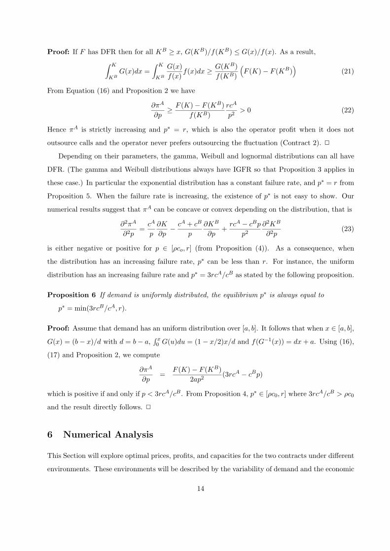
Proof: If F has DFR then for all KB ≥ x, G(KB)/f(KB) ≤ G(x)/f(x). As a result,∫ K

KBG(x)dx =

∫ K

KB

G(x)f(x)

f(x)dx ≥ G(KB)f(KB)

(F (K)− F (KB)

)(21)

From Equation (16) and Proposition 2 we have

∂πA

∂p≥ F (K)− F (KB)

f(KB)rcA

p2> 0 (22)

Hence πA is strictly increasing and p∗ = r, which is also the operator profit when it does not

outsource calls and the operator never prefers outsourcing the fluctuation (Contract 2). 2

Depending on their parameters, the gamma, Weibull and lognormal distributions can all have

DFR. (The gamma and Weibull distributions always have IGFR so that Proposition 3 applies in

these case.) In particular the exponential distribution has a constant failure rate, and p∗ = r from

Proposition 5. When the failure rate is increasing, the existence of p∗ is not easy to show. Our

numerical results suggest that πA can be concave or convex depending on the distribution, that is

∂2πA

∂2p=

cA

p

∂K

∂p− cA + cB

p

∂KB

∂p+

rcA − cBp

p2

∂2KB

∂2p(23)

is either negative or positive for p ∈ [ρco, r] (from Proposition (4)). As a consequence, when

the distribution has an increasing failure rate, p∗ can be less than r. For instance, the uniform

distribution has an increasing failure rate and p∗ = 3rcA/cB as stated by the following proposition.

Proposition 6 If demand is uniformly distributed, the equilibrium p∗ is always equal to

p∗ = min(3rcB/cA, r).

Proof: Assume that demand has an uniform distribution over [a, b]. It follows that when x ∈ [a, b],

G(x) = (b− x)/d with d = b− a,∫ x0 G(u)du = (1− x/2)x/d and f(G−1(x)) = dx + a. Using (16),

(17) and Proposition 2, we compute

∂πA

∂p=

F (K)− F (KB)2ap2

(3rcA − cBp)

which is positive if and only if p < 3rcA/cB. From Proposition 4, p∗ ∈ [ρc0, r] where 3rcA/cB > ρc0

and the result directly follows. 2

6 Numerical Analysis

This Section will explore optimal prices, profits, and capacities for the two contracts under different

environments. These environments will be described by the variability of demand and the economic

14

parameters r, cA, cB that establish the margins for each party. We consider two types of demand

variability: within period variability, which is determined by the demand distribution of a given

time period and between period variability, which refers to the demand pattern across multiple

periods, captured through the change in the parameters of a particular demand distribution. Our

first objective is to develop a general understanding of each contract under steady demand (i.e. no

between period variability). We then explore the impact between period variability has on contract

behavior. Restricting our attention to a particular level of within period variability, we then explore

the role economic parameters have on these contracts. For all settings, our ultimate objective is to

address the contract choice problem posed in the Introduction: under what conditions does each

party prefer a particular contract?

Viewed in a different context, the contract choice problem resembles the outsourcing versus

contract manufacturing problem faced by OEMs in electronics, as described by Plambeck and

Taylor (2001). OEM outsourcing refers to the case where an OEM only outsources part of its

production, whereas contract manufacturing constitutes the case where the entire production is

outsourced. In a single period setting, we show that under Contract 1 all capacity is outsourced,

like in contract manufacturing, whereas under Contract 2, some capacity is kept in-house, like in

OEM outsourcing. Our numerical examples will explore the multi-period setting, and illustrate

that when there is between period demand variability both parties can invest in some capacity

under both contracts.

6.1 The role of within period variability

We consider the simplest multi-period setting with three time periods. In order to isolate the

effect of within period variability, this section considers an identical demand distribution in each

time period. For the experiments we use the Erlang family of distributions. The m-stage Erlang

distribution (referred to as Erlang-m) is completely characterized by its mean and the number of

stages m, and has the following probability density function:

f(x) =xm−1e−x/θ

θm (m− 1)!x ≥ 0

where m is positive integer and θ is a positive real number. The mean of the distribution is mθ.

Note that the Erlang-1 distribution is the simple exponential distribution. Focusing on the Erlang

family enables to systematically investigate the effect of variability since an Erlang-m distribution

is more variable than an Erlang-m’ distribution with the same mean when m′ > m according to a

15

convex stochastic order. This, naturally, implies that the variance is decreasing in m (for identical

means). Finally, Erlang distributions possess the IGFR property required by Proposition 3.

We analyze four demand distributions, Exponential, Erlang-2, Erlang-10, and Erlang-100, going

from high (H) within period variability, to low (L) within period variability. The exponential

(Erlang-1) represents a highly variable demand, the Erlang-10 resembles a Normal Distribution with

a small coefficient of variation, and Erlang-100 is used as a test case for extremely low variability.

When an identical demand distribution is assumed in each period, the multi-period problem is

structurally equivalent to the single-period problem. In order to compute the optimal capacities

we make use of Propositions 1 and 2. The optimal price for each contract is then calculated via a

numerical search (using discrete intervals of 0.01). For Contract 2, we also make use of the bounds

established in Proposition 4 to restrict the search region. Finally, for the exponential distribution

Proposition 5 directly yields the optimal price for Contract 2.

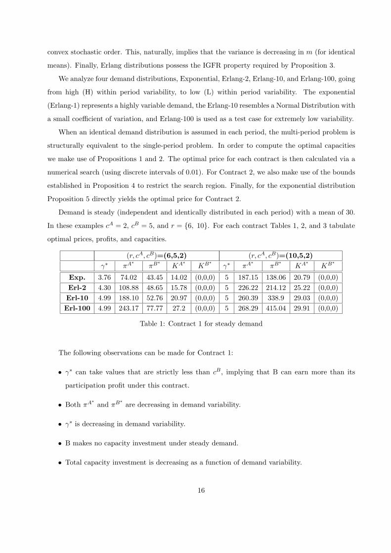
Demand is steady (independent and identically distributed in each period) with a mean of 30.

In these examples cA = 2, cB = 5, and r = {6, 10}. For each contract Tables 1, 2, and 3 tabulate

optimal prices, profits, and capacities.

(r, cA, cB)=(6,5,2) (r, cA, cB)=(10,5,2)γ∗ πA∗ πB∗ KA∗ KB∗ γ∗ πA∗ πB∗ KA∗ KB∗

Exp. 3.76 74.02 43.45 14.02 (0,0,0) 5 187.15 138.06 20.79 (0,0,0)Erl-2 4.30 108.88 48.65 15.78 (0,0,0) 5 226.22 214.12 25.22 (0,0,0)Erl-10 4.99 188.10 52.76 20.97 (0,0,0) 5 260.39 338.9 29.03 (0,0,0)Erl-100 4.99 243.17 77.77 27.2 (0,0,0) 5 268.29 415.04 29.91 (0,0,0)

Table 1: Contract 1 for steady demand

The following observations can be made for Contract 1:

• γ∗ can take values that are strictly less than cB, implying that B can earn more than its

participation profit under this contract.

• Both πA∗ and πB∗ are decreasing in demand variability.

• γ∗ is decreasing in demand variability.

• B makes no capacity investment under steady demand.

• Total capacity investment is decreasing as a function of demand variability.

16

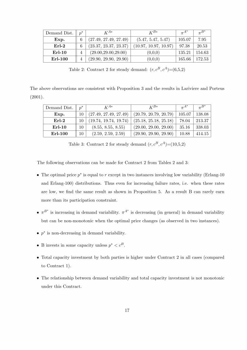
Demand Dist. p∗ KA∗ KB∗ πA∗ πB∗

Exp. 6 (27.49, 27.49, 27.49) (5.47, 5.47, 5.47) 105.07 7.95Erl-2 6 (23.37, 23.37, 23.37) (10.97, 10.97, 10.97) 97.38 20.53Erl-10 4 (29.00,29.00,29.00) (0,0,0) 135.21 154.63Erl-100 4 (29.90, 29.90, 29.90) (0,0,0) 165.66 172.53

Table 2: Contract 2 for steady demand: (r, cB, cA)=(6,5,2)

The above observations are consistent with Proposition 3 and the results in Lariviere and Porteus

(2001).

Demand Dist. p∗ KA∗ KB∗ πA∗ πB∗

Exp. 10 (27.49, 27.49, 27.49) (20.79, 20.79, 20.79) 105.07 138.08Erl-2 10 (19.74, 19.74, 19.74) (25.18, 25.18, 25.18) 78.04 213.37Erl-10 10 (8.55, 8.55, 8.55) (29.00, 29.00, 29.00) 35.16 338.03Erl-100 10 (2.59, 2.59, 2.59) (29.90, 29.90, 29.90) 10.88 414.15

Table 3: Contract 2 for steady demand (r, cB, cA)=(10,5,2)

The following observations can be made for Contract 2 from Tables 2 and 3:

• The optimal price p∗ is equal to r except in two instances involving low variability (Erlang-10

and Erlang-100) distributions. Thus even for increasing failure rates, i.e. when these rates

are low, we find the same result as shown in Proposition 5. As a result B can rarely earn

more than its participation constraint.

• πB∗ is increasing in demand variability. πA∗ is decreasing (in general) in demand variability

but can be non-monotonic when the optimal price changes (as observed in two instances).

• p∗ is non-decreasing in demand variability.

• B invests in some capacity unless p∗ < cB.

• Total capacity investment by both parties is higher under Contract 2 in all cases (compared

to Contract 1).

• The relationship between demand variability and total capacity investment is not monotonic

under this Contract.

17

The first observation implies that Contract 2 will rarely be preferred by B. Contrasting this to

the first observation for Contract 1, we expect Contract 1 to be preferred by B more frequently.

Coupled with the differences in the response of πA∗ and πB∗ to variability, we anticipate contract

choice to change as a function of demand variability. This will be explored below.

6.2 The impact of between period variability

In this section, we drop the assumption that demand is steady and consider the effect of between

period variability. The calculations are done in a similar manner using the analytical results

in combination with a numerical search for the optimal prices. Mean demands are assumed to

be (15, 60, 15). Note that the total mean demand is the same as before, however the way it is

distributed over time is different. All other parameters are the same. For each contract Tables 4,

5 and 6 tabulate optimal prices, profits, and capacities.

(r, cA, cB)=(6,5,2) (r, cA, cB)=(10,5,2)γ∗ πA∗ πB∗ KA∗ KB∗ γ∗ πA∗ πB∗ KA∗ KB∗

Exp. 3.68 52.46 32.50 10.41 (0, 0.53, 0) 4.79 136.40 138.13 16.30 (0, 25.29, 0)Erl-2 4 64.14 44.74 10.69 (0, 11.24, 0) 4.99 113.20 213.74 12.62 (0, 37.73, 0)Erl-10 4.99 94.18 52.45 10.5 (0, 31.33, 0) 4.99 130.24 338.47 14.52 (0, 43.49, 0)Erl-100 4.99 121.63 77.36 13.56 (0, 40.63, 0) 4.99 134.19 414.59 14.96 (0, 44.84, 0)

Table 4: Contract 1 under fluctuating demand

Demand Dist. p∗ KA∗ KB∗ πA∗ πB∗

Exp. 6 (13.74, 54.98, 13.74) (2.73, 10.94, 2.73) 105.07 7.95Erl-2 6 (11.68, 46.74,11.68) (5.48, 21.93, 5.48) 97.38 20. 53Erl-10 4 (14.50,58.01,14.50) (0,0,0) 135.21 154.63Erl-100 4 (14.95, 59.80, 14.95) (0,0,0) 165.66 172.53

Table 5: Contract 2 under fluctuating demand: (r, cB, cA)=(6,5,2)

Comparing the results in this Section to the previous one, we note the following:

• γ∗ is also decreasing as a function of between period demand variability.

• πA∗ and πB∗ under Contract 2 do not depend on how demand is allocated between periods.

• B invests in some capacity even under Contract 1, due to the fluctuation in demand. However

total capacity investment is still higher under Contract 2.

18

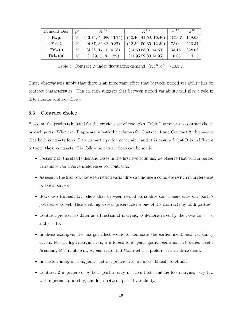
Demand Dist. p∗ KA∗ KB∗ πA∗ πB∗

Exp. 10 (13.74, 54.98, 13.74) (10.40, 41.59, 10.40) 105.07 138.08Erl-2 10 (9.87, 39.48, 9.87) (12.59, 50.35, 12.59) 78.04 213.37Erl-10 10 (4.28, 17.10, 4.28) (14.50,58.01,14.50) 35.16 338.03Erl-100 10 (1.29, 5.18, 1.29) (14.95,59.80,14.95) 10.88 414.15

Table 6: Contract 2 under fluctuating demand: (r, cB, cA)=(10,5,2)

These observations imply that there is an important effect that between period variability has on

contract characteristics. This in turn suggests that between period variability will play a role in

determining contract choice.

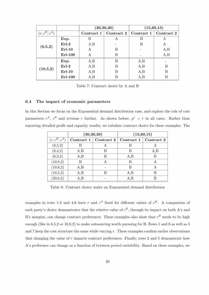
6.3 Contract choice

Based on the profits tabulated for the previous set of examples, Table 7 summarizes contract choice

by each party. Whenever B appears in both the columns for Contract 1 and Contract 2, this means

that both contracts force B to its participation constraint, and it is assumed that B is indifferent

between these contracts. The following observations can be made:

• Focusing on the steady demand cases in the first two columns, we observe that within period

variability can change preferences for contracts.

• As seen in the first row, between period variability can induce a complete switch in preferences

by both parties.

• Rows two through four show that between period variability can change only one party’s

preference as well, thus enabling a clear preference for one of the contracts by both parties.

• Contract preferences differ as a function of margins, as demonstrated by the cases for r = 6

and r = 10.

• In these examples, the margin effect seems to dominate the earlier mentioned variability

effects. For the high margin cases, B is forced to its participation contraint in both contracts.

Assuming B is indifferent, we can state that Contract 1 is preferred in all these cases.

• In the low margin cases, joint contract preferences are more difficult to obtain.

• Contract 2 is preferred by both parties only in cases that combine low margins, very low

within period variability, and high between period variability.

19

(30,30,30) (15,60,15)(r, cB, cA) Contract 1 Contract 2 Contract 1 Contract 2

(6,5,2)

Exp.Erl-2Erl-10Erl-100

BA,BAA

A-BB

BB--

AAA,BA,B

(10,5,2)

Exp.Erl-2Erl-10Erl-100

A,BA,BA,BA,B

BBBB

A,BA,BA,BA,B

-BBB

Table 7: Contract choice by A and B

6.4 The impact of economic parameters

In this Section we focus on the Exponential demand distribution case, and explore the role of cost

parameters cA, cB and revenue r further. As shown before, p∗ = r in all cases. Rather than

reporting detailed profit and capacity results, we tabulate contract choice for these examples. The

(30,30,30) (15,60,15)(r, cB, cA) Contract 1 Contract 2 Contract 1 Contract 2

(6,5,2) B A B A(6,4,2) A,B B B A,B(6,3,2) A,B B A,B B(10,8,2) B A B A(10,6,2) A,B - B A(10,5,2) A,B B A,B B(20,6,2) A,B - A,B B

Table 8: Contract choice under an Exponential demand distribution

examples in rows 1-3 and 4-6 have r and cA fixed for different values of cB. A comparison of

each party’s choice demonstrates that the relative value of cB, through its impact on both A’s and

B’s margins, can change contract preferences. These examples also show that cB needs to be high

enough (like in 6,5,2 or 10,8,2) to make outsourcing worth pursuing for B. Rows 1 and 6 as well as 5

and 7 keep the cost structure the same while varying r. These examples confirm earlier observations

that changing the value of r impacts contract preferences. Finally, rows 2 and 5 demonstrate how

A’s preference can change as a function of between period variability. Based on these examples, we

20

can state that all economic parameters have an important role in determining contract choice by

defining profit margins available to each party.

6.5 Summary

The different types of demand variability that were considered are observed to have two different

effects in these examples. The within period demand variability has an impact on the optimal price.

Thus, under Contract 1, as also in Proposition 3, lower within period demand variability implies

higher γ values in equilibrium, approaching the cB upper limit. The optimal price p under Contract

2 on the other hand, approaches its upper value r for higher values of r and for environments with

high within period demand variability. Whenever p = r or γ approaches cB the operator earns

profits equal to the case when everything is performed in-house. As a result, whenever price is at its

upper-bound for one contract, the operator prefers outsourcing with the other contract. This is so

as long as the other contract enables an optimal price p or γ that is below their upper bound values.

When γ∗ = cB and p∗ = r, γ∗ < p∗ so that for such a case Contract 1 with subcontracting the

base is preferred by the operator. The contractor’s preference also depends on the between period

variability effect. Indeed we find both in some low within period, low revenue cases and some high

within period, high revenue cases that the contractor’s preference switches from one contract to

the other as a function of the between period demand variability. This example underlines the

importance of considering the multi-period effect in such outsourcing contract choice problems.

Our examples demonstrate that contract choice depends on between period demand fluctuations,

as our operations management intuition would suggest, but also on the within period demand

variability through its effect on pricing. Similarly economic parameters, through their effect on the

optimal pricing decision, impact this choice. Thus the operator’s choice of Contract 1 turns out to

be also the contractor’s choice in high margin settings, or under particular variability conditions

when margins are low. In the example, total capacity investment by the operator and contractor

in each period is higher under Contract 2, thus customer service is better when this Contract is

preferred by both parties. However conditions that ensure this are found to be quite restrictive.

Despite our initial intuition that the contract which subcontracts the fluctuation is structurally

more appropriate for a setting where the contractor’s capacity cost is lower, due to pricing effects

(driven in part by within period variability) this contract is not preferred by both in most settings.

As is also evident from Proposition 1, in the multi-period setting with fluctuating demand, the

operator may choose to invest in capacity under both contracts. Thus we find that the between

21

period variability effect can induce a switch from a contract manufacturing to outsourcing type of

solution in the electronics manufacturing context. For call centers, our examples suggest that both

contract types will lead to a co-sourcing solution whereby calls are shared by both parties in most

cases. Unless call volumes are steady across periods (under Contract 1) or within period variability

and margins are low (under Contract 2), B will not prefer to outsource all calls to A.

In summary, we find that none of the contracts are universally preferred, and that preferences

change as a function of within period variability, between period variability, and profit margins

determined by the values of r, cA, and cB. Our results further demonstrate that the pricing

decision plays an important role in this choice, and that taking price as an exogenously given

parameter could be misleading. The analysis points to the need for a good understanding of the

operating environment of service companies, before contract decisions are made for outsourcing.

7 Concluding Remarks

This paper is the first to model call center outsourcing contracts, and to explore these in terms of

design and contract choice. While the motivating example came from a call center, the results would

also be applicable to other types of service outsourcing like the outsourcing of back-office functions.

Key distinguishing features of the model are the presence of multiple decision makers, uncertain

demand, endogenous pricing decisions, and a multi-period decision horizon. We find that all of

these features have an important impact on the contract choice problem, and that the qualitative

nature of the results change as a function of these features. This points to the importance of taking

them into account in answering questions about service outsourcing contracts. From a modeling

standpoint, one can conclude that the endogenous pricing feature is the one that complicates the

analysis the most. Whenever the outsourcing vendor is a price taker, our analysis fully characterizes

both contracts.

For managers who face these types of contract design and choice problems, our analysis demon-

strates that in addition to a knowledge of economic parameters like costs, managers need to have

a very good understanding of the underlying demand uncertainties. None of the contracts are pre-

ferred under all conditions, and different choices lead to different outcomes in terms of profits and

customer service provided. Evaluation of different contract choices should not be simplified to a cost

per transaction basis. Our analysis suggests that when margins are relatively high, subcontracting

the base is preferred by both parties. Subcontracting the fluctuation is only preferred by both

22

parties when margins are low, inherent demand variability is low but between period fluctuations

are high. Since this contract typically leads to higher capacity investment, further research may

explore hybrid contracts that ensure these high service levels as well as preference by both parties

under more general conditions.

References

Anupindi, R. and Bassok, Y. (1998) “Supply Contracts with Quantity Commitments and Stochastic

Demand”, in Quantitative Models for Supply Chain Management, Tayur, S., Ganeshan, R. and

Magazine, M. (eds.), p. 197

Atamturk, A. and Hochbaum, D. (2001) “Capacity Acquisition, Subcontracting, and Lot Sizing”,

Management Science, Vol. 47:8, 1081-1100.

Cachon, G.P. and Harker, P.T. (2003). “Competition and outsourcing with scale economies”,

Management Science, Vol. 48:10; p. 1314-1334.

Datamonitor (1999) “Outsourcing to boom in Europe”, http://resources.talisma.com/ver call statistics.asp

Dong, L. and Rudi, N. (2004). “Who Benefits from Transshipment? Exogenous vs. Endogenous

Wholesale Prices”, Management Science, Vol. 50:5; p. 645-658.

Fuhrman, F. (1999). “Co-sourcing: A winning alternative to outsourcing call center operations”,

Call Center SolutionsVol. 17:12; p. 100-103.

Gans, N. and Zhou, Y. (2004) “Overflow Routing for Call Center Outsourcing”, Working Paper,

The Wharton School.

Gans, N., Koole, G. M. and Mandelbaum, A. (2002), ”Telephone Call Centers: Tutorial, Review,

and Research Prospects, Manufacturing & Service Operations Management, vol. 5, pp. 97-141.

Gopal, A. Sivaramakrishnan, K., Krishnan, M.S. and Mukhopadhyay, T. (2003). “Contracts in

Offshore Software Development: An Empirical Analysis”, Management Science, Vol. 49:12; pp.

1671-1683

International Data Corporation, (June 1999), http://www.callcenternews.com/resources/stats size.shtml

Kalnins, A.(2004). “Relationships and Hybrid Contracts: An Analysis of Contract Choice in

Information Technology”, Journal of Law Economics and Organization, Vol. 20:1; p. 207.

Kamien, M.I., Li, L., and Samet, D. (1989). “Bertrand competition with subcontracting”, RAND

Journal of Economics Vol. 20:4, pp. 553-567.

Kamien, M.I. and Li, L. (1990). “Subcontracting, Coordination, Flexibility, and Production

Smoothing in Aggregate Planning”, Management Science, Vol. 36:11, pp. 1352-1363

23

Lacity, M.C. and Willcox, L.P.(2001) Global Information Technology Outsourcing: In Search of

Business Advantage, John Wiley and Sons Ltd, Chicester, England.

Lariviere, M.A. (1998), “Supply Chain Contracting and Coordination with Stochastic Demand”,

in Quantitative Models for Supply Chain Management, Tayur, S., Ganeshan, R. and Magazine, M.

(eds.), p. 233.

Lariviere, M. A. and Porteus, E.L. (2000) “Selling to the Newsvendor: An Analysis of Price-Only

Contracts” Manufacturing & Service Operations Management. Vol. 3:4; p. 293-306.

Plambeck, E.L. and Taylor, T.A. (2001) “Sell the Plant? The Impact of Contract Manufacturing

on Innovation, Capacity, and Profitability”, forthcoming, Management Science.

Tan, B. (2002) “Managing Manufacturing Risks by Using Capacity Options”, Journal of the Op-

erational Research Society, 53; p. 232-242.

Tsay, A.A., Nahmias, S., and Agrawal, N. (1998) “Modeling Supply Chain Contracts: A Review”,

in Quantitative Models for Supply Chain Management, Tayur, S., Ganeshan, R. and Magazine, M.

(eds.), p. 299.

Van Mieghem, J.A. (1999). “Coordinating investment, production, and subcontracting”, Manage-

ment Science Vol. 45:7; p. 954:972.

24