Syracuse University Syracuse University

SURFACE SURFACE

Theses - ALL

June 2019

Capturing and analyzing multispectral UAV imagery to delineate Capturing and analyzing multispectral UAV imagery to delineate

submerged aquatic vegetation on a small urban stream submerged aquatic vegetation on a small urban stream

Riley Sessanna Syracuse University

Follow this and additional works at: https://surface.syr.edu/thesis

Part of the Physical Sciences and Mathematics Commons

Recommended Citation Recommended Citation Sessanna, Riley, "Capturing and analyzing multispectral UAV imagery to delineate submerged aquatic vegetation on a small urban stream" (2019). Theses - ALL. 354. https://surface.syr.edu/thesis/354

This Thesis is brought to you for free and open access by SURFACE. It has been accepted for inclusion in Theses - ALL by an authorized administrator of SURFACE. For more information, please contact surface@syr.edu.

Abstract

For decades, remote sensing has been used by scientists and planners to make detailed observations and decisions on areas with industrial problems, remediation and development sites, and resource management. It is challenging to make high spatial and temporal resolution observations along headwater and small streams using traditional remote sensing methods, due to their high spatial variability and tendency for rapidly changing water quality and discharge. With improved technology in sensors and launching platforms, remote sensing via Unoccupied Aerial Vehicles (UAVs) now allows for imagery to be collected at high spatial and temporal resolution, with the goal of providing a deeper analysis of these intricate and difficult to access regions. One recent area of interest is the use of UAVs to delineate land and water cover. While recent innovations in low-altitude multispectral and hyperspectral imagery have been used extensively for tracking land cover, it has been used less frequently to detect changes within the water column through space and time. In addition, it is unclear whether classification methods applied to headwater systems are translatable across adjacent stream reaches or across flights on different days, as well as how much information is needed to perform such classifications. This study demonstrates that UAV multispectral imagery can be used to classify land cover as well as uniquely identify submerged aquatic vegetation by combining methods of remote sensing, image processing and machine learning. A linear discriminant analysis (LDA) model was developed to provide land and water cover classification maps (with statistical analysis of error) using training data from hand delineated multispectral shapefiles. This method proved to be robust when classifying land cover along a single reach, even when using a very small proportion of the training data. Through attempts to transfer data through space and time, this exercise highlights the shortcomings in multispectral imagery and the dependence on lighting conditions, reach orientation and shading from nearby structures such as vegetation. Therefore, this approach is likely most beneficial for classifying land cover and submerged aquatic vegetation at a single reach for a single time, but more work must be done to further identify physical limitations of multispectral imagery and calibration methods which might allow for an “absolute” measure of reflectance.

Capturing and analyzing multispectral UAV imagery to delineate submerged aquatic vegetation on a small urban stream

By

Riley Sessanna

B.A. SUNY Geneseo, 2017

THESIS

Submitted in partial fulfillment of the requirements for the degree of Master of Science in Earth Sciences

Syracuse University

June 2019

Copyright © Riley Sessanna, June 2019 All Rights Reserved

iv

Acknowledgements

This Master’s Thesis aims to better understand the utility and limitations of UAV-

multispectral imagery in classifying in stream, submerged aquatic vegetation as well as

surrounding land cover. This research would not have been possible without the help of many

people that I have met in both my personal and academic life. First of all, I would like to thank

my parents and family for raising me to always ask questions and giving me the drive to seek out

the answers. I would like to thank the full Geology/Earth Science department at both SUNY

Geneseo and Syracuse University, where I have always felt comfortable asking for help, where

my love for the sciences has grown far beyond what I had ever imagined, and where I have met

some of my closest friends. I would like to thank Dr. Christa Kelleher, who has been my biggest

supporter at Syracuse University and helped me develop the tools and skills necessary to become

a great scientist. I would like to thank Dr. Laura Lautz, who helped me develop statistical

analysis methods which were crucial to this project, and Dr. Charles Driscoll, who always gave

support and advisement to help me move forward. I would also like to thank Ian Joyce and

Jacqueline Corbett who played an instrumental part in my field work and are the root to my

knowledge and skills with UAVs. Lastly, I would like to thank the National Science Foundation

and the EMPOWER program at Syracuse University whose funding made this project possible.

v

Table of Contents

1.0 Introduction…………………………………………………………………………………...1

2.0 Study Area…………………………………………………………………………………...4

3.0 Methods……………………………………………………………………………………...5

3.1 Flight Planning and Data Collection………………………………………………....5

3.2 Image Radiometric Calibration and Mosaicking…………………………………….6

3.3 Automated Land Cover Delineation via Linear Discriminant Analysis……………..7

3.4 Is the Model Robust through Space and Time?...........................................................9

4.0 Results………………………………………………………………………………………..10

5.0 Discussion……………………………………………………………………………………12

5.1 Is there Novelty in UAV Submerged Vegetation Classification?...............................12

5.2 What are the Capabilities of this Data Collection-Analysis Technique?....................13

5.3 Does this Model Transfer through Space and Time?..................................................14

5.4 Is UAV-Multispectral Data Collection a Universal Tool for all Projects?.................16

6.0 Conclusion…………………………………………………………………………………...17

7.0 Figures……………………………………………………………………………………….18

8.0 Appendix…………………………………………………………………………………….25

9.0 References…………………………………………………………………………………...33

vi

List of Figures

Figure 1

Study Site………………………………………………………………………...18

Figure 2

Methods………………………………………………………………………......19

Figure 3

LDA Land Cover Classification of Reach 1, July 16……………………………20

Figure 4

Ten-fold Cross Validation for Each Reach for Three Flight Dates……………...21

Figure 5

LDA Classification using Limited Training Data ……………………………….22

Figure 6

Ten-fold Cross Validation using Combined Spatial and Temporal Data………..23

Figure 7

Solar Radiation Measurements at the Time of Each UAV Flight……………….24

vii

Appendix

Table A1

Spatial Resolution………………………………………………………………..25

Table A2

Full Training Dataset…………………………………………………………….26

Table A3

Total Number of Pixels Classified……………………………………………….27

Table A4

10-fold Cross Validations for Variable Training Data Size……………………...27

Figure A5

Normalized Area of Submerged Aquatic Vegetation……………………............28

Figure A6

Formation of Training Dataset…………………………………………………...29

Figure A7

Distribution of Training Data by Scores for July 16……………………………..30

Figure A8

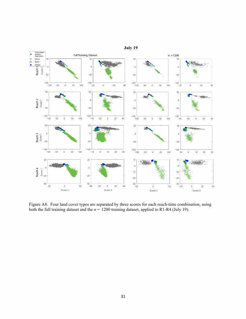
Distribution of Training Data by Scores for July 19……………………………..31

Figure A9

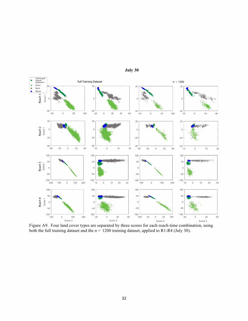
Distribution of Training Data by Scores for July 30…………………………….32

1

1.0 Introduction

Remote sensing has revolutionized our ability to observe the Earth’s surface. In

particular, technological advances in the past decade have enabled increasingly detailed temporal

and spatial monitoring of land and water cover through improved sensors as well as new low-

altitude launching platforms (Rogan and Chen, 2004; Blaschke, 2010; Watts et al., 2012; Akar,

2017). Historically, remote sensing techniques (e.g., satellite, airborne) have been used to

delineate locations of headwater and other small streams (Martz and Garbrecht, 1992; Wechsler,

2007; Kayembe and Mitchell, 2018), however due to spatial resolution, remotely sensed imagery

has not been used for other applications in these areas. Instead, stream surveys of water quality

and other in situ conditions have typically been performed by hand and on foot (e.g., Dai et al.,

2001; Ledford et al., 2017), which can make it more challenging to capture “hot spots” or “hot

moments” (e.g., McClain et al., 2003; Vidon et al., 2010), or to rapidly observe or map features

within or below the water column (e.g., submerged aquatic vegetation, stream morphology).

Conditions are especially challenging in urban environments, where changes in stream water

quality or streamflow occur over a matter of minutes (Paul and Meyer, 2001; Chen et al., 2015).

High spatial resolution (< 0.5 m) imagery is needed to make meaningful observations in

headwater environments, given the small scale of these (Marcus et al., 2003; Feurer et al., 2008).

To address challenges regarding the rapid and high resolution collection of spatial

datasets, Unoccupied Aerial Vehicles (UAVs), more commonly referred to as drones, are being

increasingly adopted for use in scientific studies (Nebiker et al., 2008; Haala et al., 2011; Gago et

al., 2015; Webster et al., 2018). UAVs can be flown within tens of meters above ground level,

enabling the collection of high-resolution data along headwater streams (Flener et al., 2013;

2

DeBell et al., 2015). The low cost of UAVs enables temporally and spatially flexible

observation schemes due to the ease of deployment and utilization, facilitating the acquisition of

large amounts of data that enable a more thorough understanding of the heterogeneity of water

quality (Dent and Grimm, 1999; Feng et al., 2015).

When it comes to translating UAV datasets into meaningful understanding of headwater

stream water quality, the primary methodological challenges have resulted in two open

questions: (1) how much data are needed to create translatable approaches that relate UAV

imagery to a metric of interest (e.g., chlorophyll, Elarab et al., 2015; turbidity, Ehmann et al.,

2018; land cover mapping, Kalantar et al., 2017), and (2) are relationships between UAV

imagery and in situ observations translatable through space and through time? When it comes to

the latter, developing translatable relationships may be influenced by weather conditions during

UAV acquisition (Zeng et al., 2017), typically treated via standard imagery calibration

approaches applied after imagery is collected, as well as variations in physical conditions

through space (e.g., shadows from trees, stream orientation) (Ishida et al., 2018; Tu et al., 2018).

The goal to create a universal and translatable algorithm between in situ observations of water

quality and variations in UAV imagery would enable ongoing monitoring via UAV with minimal

image post processing.

Land cover classification techniques usually treat water as a homogenous class (Mancini

et al., 2016; Natesan et al., 2018; Rusnák et al., 2018), or ignore the delineation of water

(Ahmed et al., 2017; Akar, 2017; Ishida et al., 2018). Here, I provide an in-depth analysis of

land cover classification, with an alternative statistical analysis approach to traditional methods

such as Rotation Forest (Akar, 2017), Random Forest (Ahmed et al., 2017) or Fast k-means

algorithms (Mancini et al., 2016). I also aim to expand on previous studies that have

3

acknowledged the heterogeneity in the “water class” by using multispectral sensors that go

beyond visual light imagery (e.g. Flynn and Chapra, 2014) in identifying vegetation not only on

the surface of water, but submerged within the water column (e.g. Husson et al., 2016), using

imagery collected via UAV platform rather than satellite or plane (e.g. Cho et al., 2008).

My application focuses on the development of a robust method for identifying and

separating the presence of submerged aquatic vegetation within the water column of a shallow

urban stream from open water as well as stream-adjacent land cover. While UAVs have been

used to improve understanding of numerous water quality applications, one primary challenge is

to determine whether objects submerged within the water column - such as nuisance algae,

milfoil, or channel bottom vegetation - can be observed via low altitude remote sensing (Flynn

and Chapra, 2014; Chirayath and Earle, 2016; Husson et al., 2016). To test capabilities for

classifying submerged aquatic vegetation in the presence of environmental variability, I collected

UAV imagery using a widely available multispectral camera imaging four common bands along

four reaches spanning a small urban stream. Imagery was collected across three flight dates. To

classify land cover, imagery was statistically analyzed using Linear Discriminant Analysis

(LDA), a method adapted to this study that uses a complete dataset to train a model that

maximizes separation between land cover classes for known land cover. Statistical LDA models

were then used to assign decision regions that enable classification of unknown pixels based on

their reflectance for each of several spectral bands.

While UAVs are being widely adopted for scientific studies, it is not clear whether the

imagery obtained from these tools is robust to environmental variability introduced during data

collection (Zeng et al., 2017). In particular, UAV imagery is impacted by differences in

environmental conditions from data collected months, weeks, days, or even minutes apart. This

4

variability is integrated across different reach orientations and characteristics. In this sense, I use

this case study of land cover classification along a headwater stream to determine whether (or

not) it is possible to develop a robust method for separating time-varying in-stream conditions,

specifically submerged aquatic vegetation, from other land cover types. Ideally, a method

capable of identifying submerged vegetation would require minimal data with limited extent and

from a single time, and would be translatable to other down- or upstream areas as well as

imagery collected on alternative dates. The major objectives to be addressed in this study are:

(1) to determine how much information is required to classify submerged aquatic vegetation

along a single reach at a single time, (2) to determine if statistical models based on UAV imagery

can be transferred in space and time to successfully separate submerged vegetation from other

types of vegetation and land cover, and (3) to determine if these statistically-based relationships

are (most) robust through space or through time.

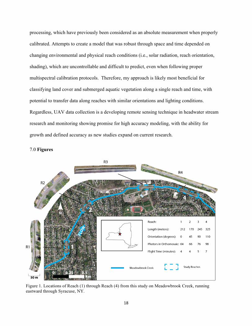
2.0 Study Area

Meadowbrook Creek is a first order stream running eastward through Syracuse, NY

(Figure 1). The stream first emerges from a retention basin before traveling 5.6 km to an Erie

Canal feeder channel (Ledford and Lautz, 2015). The upper 4.1 km of stream is highly

urbanized with armored banks that disconnect the stream from natural groundwater influx. This

channelized section has minimal riparian vegetation and is strongly influenced by road runoff

(Ledford et al., 2016). The lower 1.5 km of Meadowbrook Creek is not channelized or armored,

allowing the stream to meander through a large cemetery before entering 500 m of riparian

floodplain.

5

I identified four reaches, further referred to as R1, R2, R3, and R4, along the upstream,

urbanized portion of Meadowbrook Creek based on length and overhead accessibility to ensure

that maximum aerial imagery could be collected from a UAV during a single flight. All reaches

are between 170 and 325 meters in length and between 1.5 and 3.5 meters in width, with

recorded water depth ranging from 10 cm to 60 cm, although water levels may surpass this range

with high intensity rain events or with the scheduled release of the retention basin. Although all

reaches are surrounded by urbanized land cover, they have heterogeneous shading from canopy

cover and differing reach orientation. Importantly, growth of submerged aquatic vegetation

reflects variance in exposure to sunlight as well as nutrient input from urban processes such as

lawn fertilization, leaking sewer systems, and road runoff. Presence of submerged vegetation

varies among reaches, and represents a changing condition within the stream channel which is

measureable through UAV imagery and has ties to water quality. It is typically at a minimum

biomass in winter, begins to develop in April or May, and reaches a maximum biomass in late

July or August.

3.0 Methods

3.1 Flight Planning and Data Collection

I collected imagery using a Sequoia Multispectral Camera and Sunshine Sensor (Parrot

Drones SAS) attached via 3D printed plastic harness to a DJI Inspire 1 UAV. The camera

collects 16 Megapixel visual light (RGB) images, as well as individual Tagged Image Format

(TIF) files corresponding to green, red, red edge, and near infrared bands (center wavelengths

and bandwidths of 550 ± 20, 660 ± 20, 735 ± 5, 790 ± 20 nm, respectively). The Sunshine

Sensor continuously monitors in-flight lighting conditions in the same bands as those recorded

6

by the multispectral sensor in order to calibrate the Sequoia camera for collection of precise

imagery regardless of changing light conditions.

All missions were flown at 30 m above ground level to guarantee clearance above trees

and power lines. The Inspire 1 was set to fly at eight km hr-1, to ensure images were collected at

nearly nadir to limit distortion. For each reach, the UAV heading was set parallel to the reach

orientation and set to fly up one side of the stream and back down the opposite side, creating a

grid pattern with both image frontlap and sidelap upwards of 85%. To maintain 70 to 80%

overlap, the camera was set to collect multispectral images in the green, red, red edge, near

infrared (NIR), and RGB bands every three seconds. These flights typically began at 11:00 am

at the most upstream R1, and continued on to downstream reaches. This timing was selected to

best constrain changing lighting conditions based on sun position. I collected images of a

MicaSense Calibrated Reflectance Panel before and after each individual flight; these images

were used to radiometrically correct images for inevitably changing lighting conditions.

Missions were repeatedly flown following this protocol every one to two weeks from April 23,

2018 through July 30, 2018. For this particular study, I focus on imagery collected on three

dates: July 16, July 19, and July 30, 2018.

3.2 Image Radiometric Calibration and Mosaicking

Images were corrected and post-processed in Pix4D (v. 4.4.4) software, which was used

to build georeferenced RGB, green, red, red edge, and NIR orthomosaics across four reaches for

three flights per reach. Pix4D uses the in-flight records of lighting conditions recorded by the

sunshine sensor to normalize images, and employs the radiometric calibration target as an

absolute reference to correct for changing lighting conditions between flights. When combined,

the sunshine sensor and calibration target allow for in-flight and absolute correction of

7

reflectance values while the georeferenced orthomosaics are built. Spatial resolution of the

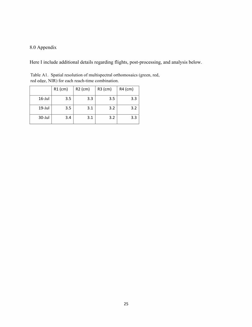
multispectral orthomosaics ranged from 3.1 to 3.5 cm (Appendix Table A1).

3.3 Automated Land Cover Delineation via Linear Discriminant Analysis

Linear Discriminant Analysis (LDA) is a statistical method that seeks user input for

dimensionality reduction and classification (James et al., 2013). LDA relies on a complete

training dataset, that includes continuous data for multiple variables with classifications of

observations in pre-defined groups. These data are used to create dependent variables

(discriminants, or scores) that are the linear combination of the multivariable input data. These

dependent variables summarize the data while also creating maximum separation between

classes of data, and minimum separation within individual classes. Scores are created based on

an n – 1 (degrees of freedom minus one) basis, with each score representing an additional plane.

In this study, four land cover types are represented by three scores in a three dimensional plane.

To build an algorithm that relates submerged aquatic vegetation cover to spectral

signatures, I imported reach orthomosaics into ArcMap (v. 10.5.1) and used RGB imagery to

guide hand delineation of four different types of land cover: submerged aquatic vegetation, open

water, grass, and rock. These classes represent the four main types of common land cover that I

identified across stream reaches and the approximately 2 meters of land cover surrounding each

reach. I define these covers more specifically as follows:

• Submerged aquatic vegetation – aquatic non-rooted vegetation with bounds

constrained within the aqueous stream channel,

• Grass – all regions of soil and vegetation consisting of short, narrow leaves

beyond the bounds of the aqueous stream channel,

8

• Rock – all consolidated material not inundated with water which does not consist

of soil or vegetation, and

• Open water – all regions within the stream channel which do not contain

submerged aquatic vegetation, other types of vegetation, or rock.

All LDA models require a training set – representing known group classifications and

their corresponding data – as input to generate statistical relationships used to classify unknown

pixels. To create an unbiased training dataset, land cover shapefiles were randomly delineated

throughout each reach (Appendix Figure A6) and used to mask each reflectance band based on

the four land cover types above. Pixel reflectance was exported from ArcGIS for these four land

cover types and summarized in a table of reflectance values for each band indexed by cover type.

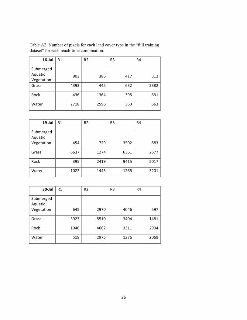
I refer to these data as the “full training dataset” – it contains all of the information from the

original masking shapefiles, without any trimming or constraints on the number of training pixels

included in the LDA model (Appendix Table A2). There are 12 “full training datasets” included

in this study, one for each reach-time combination.

From the training dataset, I applied LDA to derive a linear relationship that maximized

separation between the four cover types on a three-dimensional plane (Appendix Figure A7, A8,

A9). LDA relationships consisted of three linear discriminant classifiers (the number of

classification groups less one) computed as a coefficient plus the summation of the green, red,

red edge, and NIR reflectance bands each weighted by a loading factor. Ten-fold cross

validation was performed during each model run to test model accuracy by determining the

percentage of misclassified pixels (losses). LDA discriminants were then used to classify all

unknown pixels on each reach as either submerged aquatic vegetation, grass, rock or water.

9

As the development of a training dataset requires hand delineation of land cover types,

this resulted in an uneven number of pixels of a certain land cover per site, and different sizes of

training datasets across sites and flights. To identify a common dataset size and to determine

how much data are needed to create a robust model, I curated and varied the training dataset

within the LDA approach for R1 on July 16. I created subsets of the training dataset that

consisted of a 1:1 ratio among all four types of land cover, and reran the model five times, each

time putting stricter limits on the total number of pixels to be included in the training data (n =

1600, n = 1200, n = 800, n = 400, n = 200). For each n, I created 100 training datasets randomly

sampled from the full training dataset that were used to classify pixels along the entire reach as

one of the four types of land cover. Pixels that did not change classification throughout the 100

iterations were considered to have 100% classification consistency. Ten-fold cross validation

was also performed resulting in the average loss, or percentage of misclassified pixels, for each

iteration. A common dataset size of n = 1200 pixels was then created for each reach-time

combination from each full training dataset.

3.4 Is the Model Robust through Space and Time?

If land cover spectral signals are unique, LDA models developed for one reach should be

transferable to other reaches and for imagery collected at different times. To test model

transferability through space, I combined reflectance values for all four of our study reaches

from a single date. Similarly, to test the model’s transferability through time, I combined

reflectance values from all three of the study dates for a single reach. Patterns through space and

time were compared to solar radiation data collected at the Syracuse University weather station

throughout the study period (“Syracuse University WeatherSTEM,” n.d.).

10

4.0 Results

Weather across the flight dates from mid to late July was warm, with storms occurring

between flight dates. Average daily air temperatures ranged from 20˚C to 29 ˚C. This period was

also wet, with storms delivering 1.2 cm of precipitation between the July 16 and July 19 flights,

and a total of 2.3 cm of precipitation from July 22 to July 27, prior to the July 30 flight.

The full training datasets were used without any trimming to first determine if LDA could

generate robust and accurate classifications. Discriminants produced from model runs using the

full training datasets for individual reaches and flight dates were used to classify between

1,284,172 and 3,523,431 pixels per reach, per flight (Appendix Table A3). An example of this

classification is shown in Figure 3 for R1 (July 16), with classification presented alongside RGB

imagery. The percentage of misclassified pixels from the 10-fold cross validation varied from

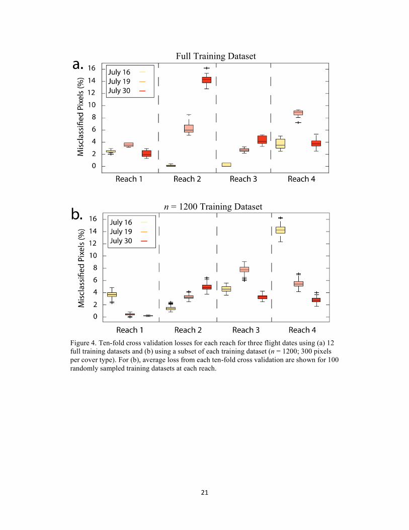
0% (R2, July 16) to 16.2% (R2, July 30). These values are summarized in Figure 4(a).

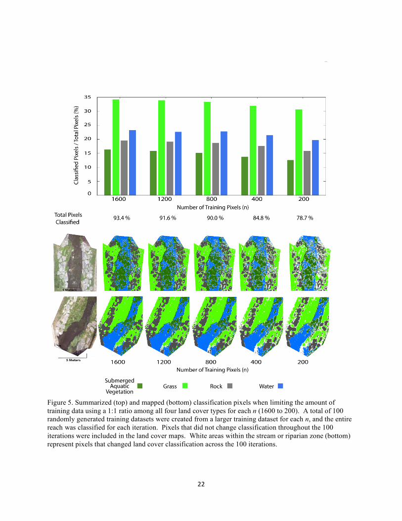
To test the limitations of my classification, I randomly subsampled the R1 (July 16) full

training dataset to only include a specified number of training pixels from each land cover type,

applied solely to R1. This exercise allowed me to assess how classification accuracy varied with

training dataset size. Limiting the number of training data to n = 1600 resulted in 100%

classification consistency (i.e., pixels that did not change land cover classification over 100

iterations) for 93.4% of the pixels along R1 (July 16), with an average loss of 3.7% for the 10-

fold cross validation (Appendix Table A4). Further limiting the training dataset to n = 1200 (300

pixels per cover type), n = 800 (200 pixels per cover type), n = 400 (100 pixels per cover type)

and n = 200 (50 pixels per cover type) resulted in greater percentages of unclassified pixels (i.e.,

pixels that changed land cover classification over 100 iterations). However, this application of

LDA yielded 100% classification consistency of nearly 80% of the 1,284,172 total pixels along

11

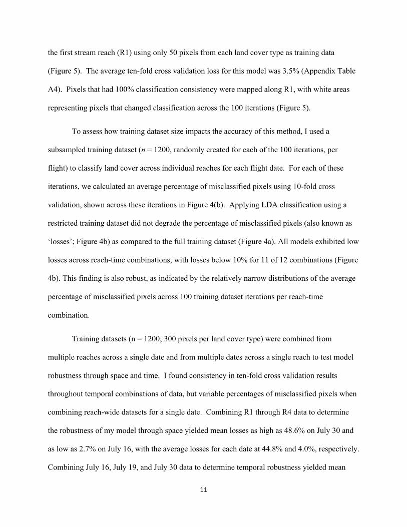
the first stream reach (R1) using only 50 pixels from each land cover type as training data

(Figure 5). The average ten-fold cross validation loss for this model was 3.5% (Appendix Table

A4). Pixels that had 100% classification consistency were mapped along R1, with white areas

representing pixels that changed classification across the 100 iterations (Figure 5).

To assess how training dataset size impacts the accuracy of this method, I used a

subsampled training dataset (n = 1200, randomly created for each of the 100 iterations, per

flight) to classify land cover across individual reaches for each flight date. For each of these

iterations, we calculated an average percentage of misclassified pixels using 10-fold cross

validation, shown across these iterations in Figure 4(b). Applying LDA classification using a

restricted training dataset did not degrade the percentage of misclassified pixels (also known as

‘losses’; Figure 4b) as compared to the full training dataset (Figure 4a). All models exhibited low

losses across reach-time combinations, with losses below 10% for 11 of 12 combinations (Figure

4b). This finding is also robust, as indicated by the relatively narrow distributions of the average

percentage of misclassified pixels across 100 training dataset iterations per reach-time

combination.

Training datasets (n = 1200; 300 pixels per land cover type) were combined from

multiple reaches across a single date and from multiple dates across a single reach to test model

robustness through space and time. I found consistency in ten-fold cross validation results

throughout temporal combinations of data, but variable percentages of misclassified pixels when

combining reach-wide datasets for a single date. Combining R1 through R4 data to determine

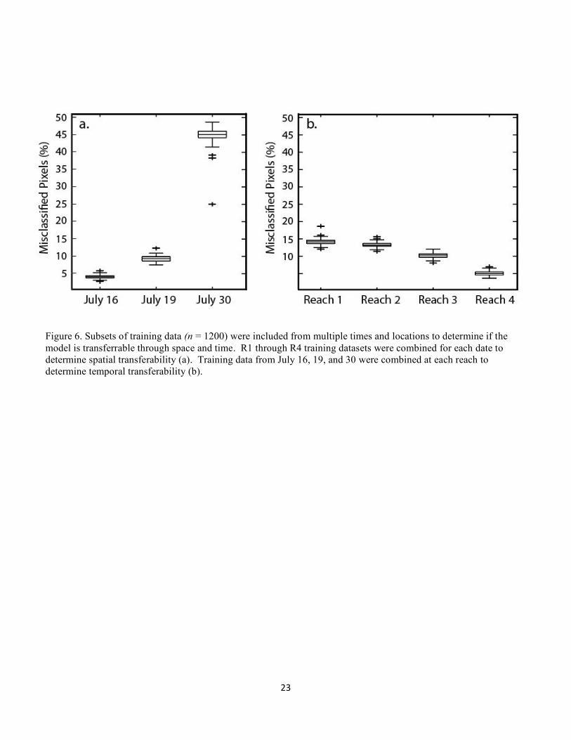
the robustness of my model through space yielded mean losses as high as 48.6% on July 30 and

as low as 2.7% on July 16, with the average losses for each date at 44.8% and 4.0%, respectively.

Combining July 16, July 19, and July 30 data to determine temporal robustness yielded mean

12

losses all below 20%, with the average loss for R1 at 14.1% and the average loss for R4 at 5.1%

(Figure 6). These findings suggest that UAV data may be more robust through time, but that

combining data from different reaches may produce a high percentage of misclassified pixels.

5.0 Discussion

5.1 Is there Novelty in UAV Submerged Vegetation Classification?

UAVs equipped with RGB, multispectral and hyperspectral sensors have been used in a

multitude of exercises to study terrain and delineate land cover (Akar, 2017; Ishida et al., 2018;

Natesan et al., 2018), a novel technique in and of itself among traditional remote sensing

approaches. Ahmed et al. (2017) found significantly higher inaccuracies in land cover and

vegetation classification when using consumer-grade RGB sensors compared to a multispectral

sensor, suggesting that a new standard may exist for data collection. To date, few research

studies have employed multispectral imagery in diverse environments. Researchers have called

for greater numbers of operational applications to diverse places and conditions to better explore

and highlight the capabilities of multispectral imagery collected from UAV platforms (Ahmed et

al., 2017). This study represents one such example seeking to expand current research

techniques and increase utility and use of these systems in land cover and vegetation

classification and monitoring. Automated classification methods following the collection of

imagery require merging approaches of remote sensing, machine learning and image processing,

creating a novelty in the combination of differing techniques between the data collection,

processing, and analysis stages of a particular project. While most techniques to classify land

cover do not separate water from submerged cover (Mancini et al., 2016; Natesan et al., 2018;

Rusnák et al., 2018), I demonstrate that it is possible to use UAV imagery to identify finer

13

features within the water column that may vary through time. While previous studies have used

RGB imagery in pursuit of similar objectives (Flynn and Chapra, 2014), my work shows that

multispectral imagery may be particularly useful for this application, and may not require much

data to achieve robust classifications of land cover.

5.2 What are the Capabilities of this Data Collection-Analysis Technique?

This system allows for the collection of inexpensive, high-resolution multispectral

imagery of a small urban stream. Collection of low altitude multispectral imagery goes beyond

fulfilling the demand for higher resolution land cover or land use mapping by providing a deeper

understanding of environmental impacts such as vegetation health and water column

heterogeneity, yielding inferences to water quality. As highlighted in this study, UAV-

multispectral systems facilitate the classification (with statistical analysis of error) of surface and

in-stream submerged cover at approximately a 3 cm spatial resolution (Figures 3 & 4, Appendix

Figure A5), with correction for spatial and temporal alterations in lighting conditions. While not

included in my study, additional analysis could incorporate more complex vegetation indices

such as Normalized Difference Vegetation Index (NDVI), Difference Vegetation Index (DVI),

and Enhanced Vegetation Index (EVI). These indices were excluded from this study for model

simplicity, but may be shown to carry additional meaning for delineating additional water

column features.

As with all models, there is a tradeoff between model complexity (e.g., the amount of

training data) and resulting output accuracy and uncertainty. To assess this tradeoff, I explored

how classification uncertainty varied with the amount of training data (Figure 5). The number of

14

training data pixels can be viewed as a proxy for ‘person-hours’ or even ‘cost’, given this

training data represents known land cover classes and therefore must be hand delineated. Even as

the size of the training dataset was restricted, I found that land cover for a large proportion of

pixels converged to a single cover class (Figure 5). This was true even for a very small training

dataset randomized across 100 iterations. If the goal of a given exercise is to achieve robust

cover classifications for all pixels, a larger training dataset should be used. However, I show that

even a small training dataset can yield robust classifications of land cover. This approach would

allow anyone employing this method to spend more time on data collection rather than

processing.

5.3 Does this Model Transfer through Space and Time?

While I show that my LDA model delineates land cover for individual reaches for a

single flight (Figure 4), the broader goal of any exercise relating multispectral imagery to land

and water cover is likely to create a model that is transferable through space and time.

Benchmarking this transferability would allow users to limit time spent in the training phase,

enabling them to hand delineate a set number of pixels at one “time” (e.g., single flight) to

repeatedly use as training data for classifying additional local sites or stream reaches. At odds

with this goal is the environmental variability found within and across stream reaches and

environmental conditions that may change from flight to flight or during a single UAV flight.

In particular, incoming irradiance measurements have been found to differ in sunlit and

shaded regions (Ishida et al., 2018), be directionally variable (Tu et al., 2018), and be affected by

sun glint on the water surface (Zeng et al., 2017). These conditions suggest it may be difficult to

transfer data collected on days with variable lighting conditions among reaches. They also hint

that transferability may be impacted by reach orientation and shading.

15

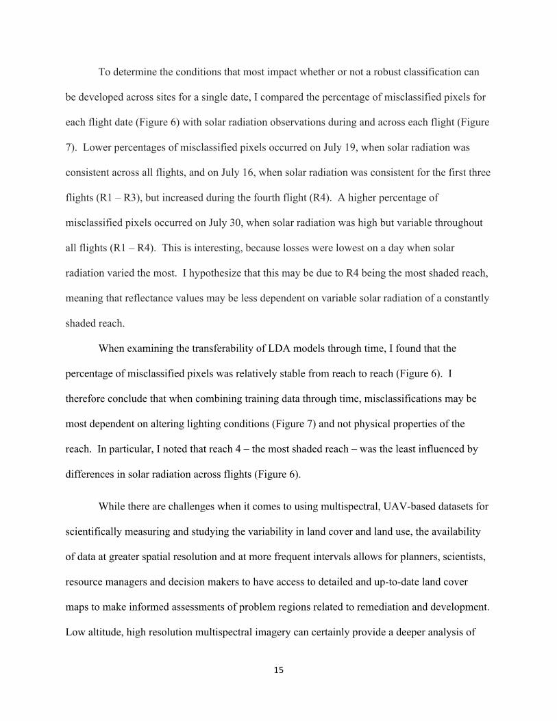
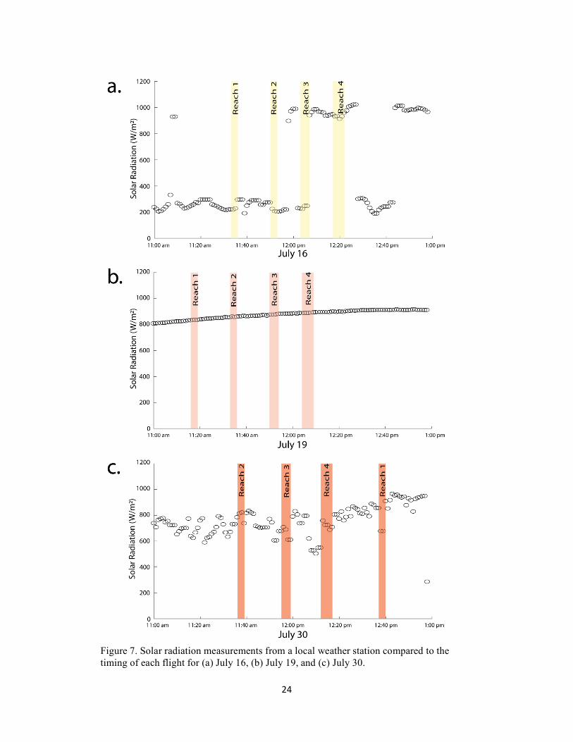
To determine the conditions that most impact whether or not a robust classification can

be developed across sites for a single date, I compared the percentage of misclassified pixels for

each flight date (Figure 6) with solar radiation observations during and across each flight (Figure

7). Lower percentages of misclassified pixels occurred on July 19, when solar radiation was

consistent across all flights, and on July 16, when solar radiation was consistent for the first three

flights (R1 – R3), but increased during the fourth flight (R4). A higher percentage of

misclassified pixels occurred on July 30, when solar radiation was high but variable throughout

all flights (R1 – R4). This is interesting, because losses were lowest on a day when solar

radiation varied the most. I hypothesize that this may be due to R4 being the most shaded reach,

meaning that reflectance values may be less dependent on variable solar radiation of a constantly

shaded reach.

When examining the transferability of LDA models through time, I found that the

percentage of misclassified pixels was relatively stable from reach to reach (Figure 6). I

therefore conclude that when combining training data through time, misclassifications may be

most dependent on altering lighting conditions (Figure 7) and not physical properties of the

reach. In particular, I noted that reach 4 – the most shaded reach – was the least influenced by

differences in solar radiation across flights (Figure 6).

While there are challenges when it comes to using multispectral, UAV-based datasets for

scientifically measuring and studying the variability in land cover and land use, the availability

of data at greater spatial resolution and at more frequent intervals allows for planners, scientists,

resource managers and decision makers to have access to detailed and up-to-date land cover

maps to make informed assessments of problem regions related to remediation and development.

Low altitude, high resolution multispectral imagery can certainly provide a deeper analysis of

16

these regions which goes beyond bulk classification of land cover, but also includes vegetation

health, diversity, and as studied in this exercise, presence within the water column (Appendix

Figure A5). This is a powerful technique which offers utility to state and federal wildlife

agencies who aim to conserve protected areas and make informed decisions following

environmental monitoring (López and Mulero-Pázmány, 2019), while also providing a high level

of reproducibility related to tasks which previously relied on observer training in correct field-

classifications, resulting in inconsistencies between observers based on level of training (Roper

and Scarnecchia, 1995).

5.4 Is UAV-Multispectral Data Collection a Universal Tool for all Projects?

When properly calibrated, multispectral data are often considered to be a high quality

measurement of reflectance across variable lighting and environmental conditions. This exercise

demonstrates the imperfections of multispectral imagery and the dependence on changing

lighting conditions, resulting in uncontrollable interactions with environmental variability along

a reach or across multiple reaches that are difficult to predict. Dependence on environmental

conditions make it difficult to transfer data through space and time, and provides useful

information to be considered when deciding what data collection platform best suits a particular

project (i.e., UAV versus plane or satellite). Although UAVs have the capability to collect high

spatial and temporal resolution data of intricate regions, they are not capable of covering the

same spatial extent (within a single image) as other platforms, introducing variability between

images collected even minutes apart. My work shows that new methodologies are needed to

reduce the impacts of environmental variability on UAV imagery, as accounting for these

17

varying conditions will likely deliver more accurate and transferable methods for use of

multispectral datasets. One complicating factor is that there is much variability and selection

introduced even before a UAV is put into the air, including the choice of heading, speed, sensor,

altitude, and time of flight; reconciling these different drivers that can all impact UAV imagery

collection will be key to improving the transferability of UAV datasets now and into the future.

6.0 Conclusions

Innovations in remote sensing are allowing scientists and planners to make meaningful

contributions to decision making regarding problem regions, remediation and development sites,

and resource management at newly improved spatial and temporal resolutions. UAVs have

recently been employed in studies to create land cover and land use maps which extend beyond

the scope of traditional methods by providing a deeper analysis of intricate and difficult to access

regions. The use of UAV multispectral and hyperspectral imagery integrated with methods in

remote sensing, image processing and machine learning now allow users to not only classify land

cover, but also identify relationships of vegetation health, diversity, and presence within the

water column through space and time.

This work presents the use of a multispectral-UAV system to classify submerged aquatic

vegetation in a small urban stream. Images were orthomosaicked and post-processed for four

separate reaches, spanning three dates. A linear discriminant analysis (LDA) model was

developed to provide land cover classification maps (with statistical analysis of error) using

training data from hand delineated multispectral shapefiles. This proved to be a robust technique

in classifying submerged aquatic vegetation for individual reaches, even when the training

dataset was restricted to a very small proportion of the original, “full training dataset.” Overall,

this work demonstrates the shortcomings in multispectral imagery collection and post-

18

processing, which have previously been considered as an absolute measurement when properly

calibrated. Attempts to create a model that was robust through space and time depended on

changing environmental and physical reach conditions (i.e., solar radiation, reach orientation,

shading), which are uncontrollable and difficult to predict, even when following proper

multispectral calibration protocols. Therefore, my approach is likely most beneficial for

classifying land cover and submerged aquatic vegetation along a single reach and time, with

potential to transfer data along reaches with similar orientations and lighting conditions.

Regardless, UAV data collection is a developing remote sensing technique in headwater stream

research and monitoring showing promise for high accuracy modeling, with the ability for

growth and defined accuracy as new studies expand on current research.

7.0 Figures

Figure 1. Locations of Reach (1) through Reach (4) from this study on Meadowbrook Creek, running eastward through Syracuse, NY.

19

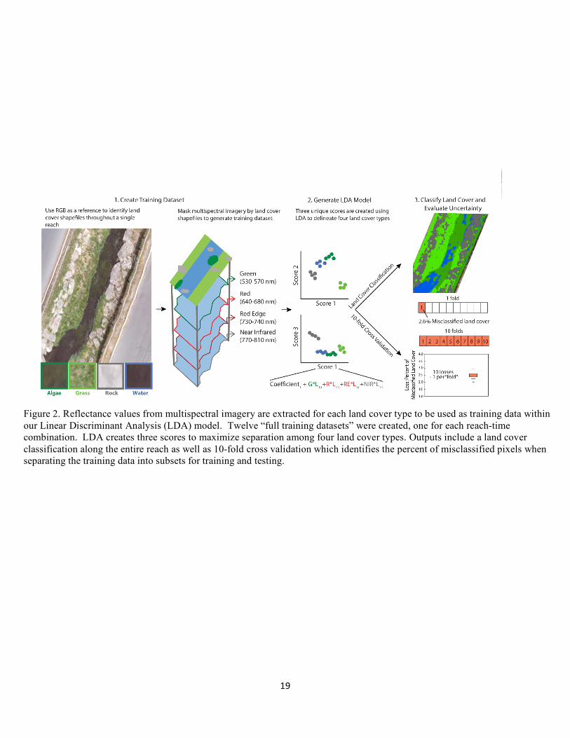
Figure 2. Reflectance values from multispectral imagery are extracted for each land cover type to be used as training data within our Linear Discriminant Analysis (LDA) model. Twelve “full training datasets” were created, one for each reach-time combination. LDA creates three scores to maximize separation among four land cover types. Outputs include a land cover classification along the entire reach as well as 10-fold cross validation which identifies the percent of misclassified pixels when separating the training data into subsets for training and testing.

20

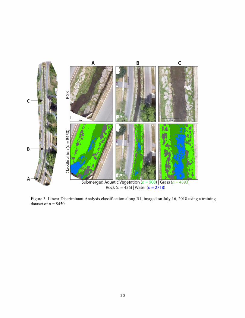
Figure 3. Linear Discriminant Analysis classification along R1, imaged on July 16, 2018 using a training dataset of n = 8450.

21

Figure 4. Ten-fold cross validation losses for each reach for three flight dates using (a) 12 full training datasets and (b) using a subset of each training dataset (n = 1200; 300 pixels per cover type). For (b), average loss from each ten-fold cross validation are shown for 100 randomly sampled training datasets at each reach.

Full Training Dataset

n = 1200 Training Dataset

22

Figure 5. Summarized (top) and mapped (bottom) classification pixels when limiting the amount of training data using a 1:1 ratio among all four land cover types for each n (1600 to 200). A total of 100 randomly generated training datasets were created from a larger training dataset for each n, and the entire reach was classified for each iteration. Pixels that did not change classification throughout the 100 iterations were included in the land cover maps. White areas within the stream or riparian zone (bottom) represent pixels that changed land cover classification across the 100 iterations.

23

Figure 6. Subsets of training data (n = 1200) were included from multiple times and locations to determine if the model is transferrable through space and time. R1 through R4 training datasets were combined for each date to determine spatial transferability (a). Training data from July 16, 19, and 30 were combined at each reach to determine temporal transferability (b).

24

Figure 7. Solar radiation measurements from a local weather station compared to the timing of each flight for (a) July 16, (b) July 19, and (c) July 30.

25

8.0 Appendix

Here I include additional details regarding flights, post-processing, and analysis below.

R1(cm) R2(cm) R3(cm) R4(cm)

16-Jul 3.5 3.3 3.5 3.3

19-Jul 3.5 3.1 3.2 3.2

30-Jul 3.4 3.1 3.2 3.3

Table A1. Spatial resolution of multispectral orthomosaics (green, red, red edge, NIR) for each reach-time combination.

26

16-Jul R1 R2 R3 R4

SubmergedAquaticVegetation

903 386 417 312

Grass 4393 445 632 2382

Rock 436 1364 395 631

Water 2718 2596 363 663

19-Jul R1 R2 R3 R4

SubmergedAquaticVegetation 454 729 3502 883

Grass 6637 1274 6361 2677

Rock 395 2419 9415 5017

Water 1022 1443 1265 3201

30-Jul R1 R2 R3 R4

SubmergedAquaticVegetation 645 2970 4046 597

Grass 3923 5510 3404 1481

Rock 1046 4667 3311 2994

Water 518 2975 1376 2069

Table A2. Number of pixels for each land cover type in the “full training dataset” for each reach-time combination.

27

R1 R2 R3 R4

16-Jul 1284172 1336779 2313206 3413042

19-Jul 1341486 1346963 3122846 3523431

30-Jul 1585657 1479372 2896613 3141530

0.0 0.5 1.0 1.5 2.0 2.5 3.0 3.5 4.0 4.5 5.0 5.5 6.0 6.5 Average n = 1600 0 0 0 0 0 0 10 42 42 6 0 0 0 0 3.7 n = 1200 0 0 0 0 0 2 14 40 31 12 1 0 0 0 3.7 n = 800 0 0 0 0 0 6 11 30 32 17 4 0 0 0 3.7 n = 400 0 0 0 0 2 4 21 14 19 23 11 5 1 0 3.8 n = 200 1 1 1 6 6 10 22 11 13 10 9 5 2 3 3.5

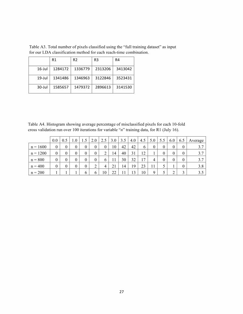
Table A3. Total number of pixels classified using the “full training dataset” as input for our LDA classification method for each reach-time combination.

Table A4. Histogram showing average percentage of misclassified pixels for each 10-fold cross validation run over 100 iterations for variable “n” training data, for R1 (July 16).

28

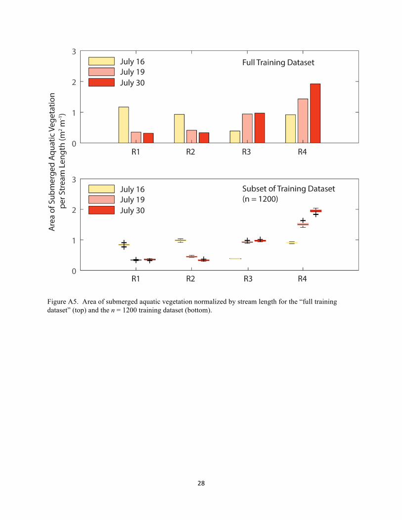
Figure A5. Area of submerged aquatic vegetation normalized by stream length for the “full training dataset” (top) and the n = 1200 training dataset (bottom).

29

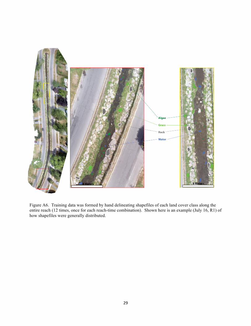
Figure A6. Training data was formed by hand delineating shapefiles of each land cover class along the entire reach (12 times, once for each reach-time combination). Shown here is an example (July 16, R1) of how shapefiles were generally distributed.

30

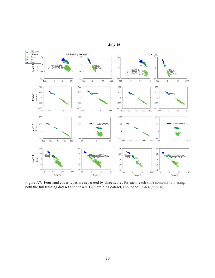
Figure A7. Four land cover types are separated by three scores for each reach-time combination, using both the full training dataset and the n = 1200 training dataset, applied to R1-R4 (July 16).

July 16

31

Figure A8. Four land cover types are separated by three scores for each reach-time combination, using both the full training dataset and the n = 1200 training dataset, applied to R1-R4 (July 19).

July 19

32

Figure A9. Four land cover types are separated by three scores for each reach-time combination, using both the full training dataset and the n = 1200 training dataset, applied to R1-R4 (July 30).

July 30

33

9.0 References

Ahmed, O. S., Shemrock, A., Chabot, D., Dillon, C., Williams, G., Wasson, R., & Franklin, S. E. (2017). Hierarchical land cover and vegetation classification using multispectral data acquired from an unmanned aerial vehicle. International journal of remote sensing, 38(8-10), 2037-2052.

Akar, Ö. (2017). Mapping land use with using Rotation Forest algorithm from UAV images. European Journal of Remote Sensing, 50(1), 269-279.

Blaschke, T. (2010). Object based image analysis for remote sensing. ISPRS journal of photogrammetry and remote sensing, 65(1), 2-16.

Chen, Y., Zhou, H., Zhang, H., Du, G., & Zhou, J. (2015). Urban flood risk warning under rapid urbanization. Environmental Research, 139, 3-10.

Chirayath, V., & Earle, S. A. (2016). Drones that see through waves–preliminary results from airborne fluid lensing for centimetre-scale aquatic conservation. Aquatic Conservation: Marine and Freshwater Ecosystems, 26, 237-250.

Cho, H. J., Kirui, P., & Natarajan, H. (2008). Test of multi-spectral vegetation index for floating and canopy-forming submerged vegetation. International journal of environmental research and public health, 5(5), 477-483.

DeBell, L., Anderson, K., Brazier, R. E., King, N., & Jones, L. (2015). Water resource management at catchment scales using lightweight UAVs: Current capabilities and future perspectives. Journal of Unmanned Vehicle Systems, 4(1), 7-30.

Dent, C. L., & Grimm, N. B. (1999). Spatial heterogeneity of stream water nutrient concentrations over successional time. Ecology, 80(7), 2283-2298.

Ehmann, K., Kelleher, C., & Condon, L. E. (2018). Monitoring turbidity from above: Deploying small unoccupied aerial vehicles to image in-stream turbidity. Hydrological Processes, 33(6), 1013-1021.

Elarab, M., Ticlavilca, A. M., Torres-Rua, A. F., Maslova, I., & McKee, M. (2015). Estimating chlorophyll with thermal and broadband multispectral high resolution imagery from an unmanned aerial system using relevance vector machines for precision agriculture. International Journal of Applied Earth Observation and Geoinformation, 43, 32-42.

Feng, Q., Liu, J., & Gong, J. (2015). Urban flood mapping based on unmanned aerial vehicle remote sensing and random forest classifier—A case of Yuyao, China. Water, 7(4), 1437-1455.

Feurer, D., Bailly, J. S., Puech, C., Le Coarer, Y., & Viau, A. A. (2008). Very-high-resolution mapping of river-immersed topography by remote sensing. Progress in Physical Geography, 32(4), 403-419.

Flener, C., Vaaja, M., Jaakkola, A., Krooks, A., Kaartinen, H., Kukko, A., ... & Alho, P. (2013). Seamless mapping of river channels at high resolution using mobile LiDAR and UAV-photography. Remote Sensing, 5(12), 6382-6407.

Flynn, K., & Chapra, S. (2014). Remote sensing of submerged aquatic vegetation in a shallow non-turbid river using an unmanned aerial vehicle. Remote Sensing, 6(12), 12815-12836.

34

Gago, J., Douthe, C., Coopman, R., Gallego, P., Ribas-Carbo, M., Flexas, J., ... & Medrano, H. (2015). UAVs challenge to assess water stress for sustainable agriculture. Agricultural water management, 153, 9-19.

Haala, N., Cramer, M., Weimer, F., & Trittler, M. (2011). Performance test on UAV-based photogrammetric data collection. International Archives of the Photogrammetry, Remote Sensing and Spatial Information Sciences, 38(6).

Husson, E., Ecke, F., & Reese, H. (2016). Comparison of manual mapping and automated object-based image analysis of non-submerged aquatic vegetation from very-high-resolution UAS images. Remote Sensing, 8(9), 724.

Ishida, T., Kurihara, J., Viray, F. A., Namuco, S. B., Paringit, E. C., Perez, G. J., ... & Marciano Jr, J. J. (2018). A novel approach for vegetation classification using UAV-based hyperspectral imaging. Computers and electronics in agriculture, 144, 80-85.

James, G., Witten, D., Hastie, T., & Tibshirani, R. (2013). An introduction to statistical learning (Vol. 112, p. 18). New York: springer.

Jiménez López, J., & Mulero-Pázmány, M. (2019). Drones for conservation in protected areas: Present and future. Drones, 3(1), 10.

Dai, K'O H., Johnson, C. E., & Driscoll, C. T. (2001). Organic matter chemistry and dynamics in clear-cut and unmanaged hardwood forest ecosystems. Biogeochemistry, 54(1), 51-83.

Kalantar, B., Mansor, S. B., Sameen, M. I., Pradhan, B., & Shafri, H. Z. (2017). Drone-based land-cover mapping using a fuzzy unordered rule induction algorithm integrated into object-based image analysis. International journal of remote sensing, 38(8-10), 2535-2556.

Kayembe, A., & Mitchell, C. P. (2018). Determination of subcatchment and watershed boundaries in a complex and highly urbanized landscape. Hydrological Processes, 32(18), 2845-2855.

Ledford, S. H., & Lautz, L. K. (2015). Floodplain connection buffers seasonal changes in urban stream water quality. Hydrological processes, 29(6), 1002-1016.

Ledford, S. H., Lautz, L. K., & Stella, J. C. (2016). Hydrogeologic processes impacting storage, fate, and transport of chloride from road salt in urban riparian aquifers. Environmental science & technology, 50(10), 4979-4988.

Ledford, S. H., Lautz, L. K., Vidon, P. G., & Stella, J. C. (2017). Impact of seasonal changes in stream metabolism on nitrate concentrations in an urban stream. Biogeochemistry, 133(3), 317-331.

Mancini, A., Frontoni, E., & Zingaretti, P. (2016, June). A multi/hyper-spectral imaging system for land use/land cover using unmanned aerial systems. In 2016 International Conference on Unmanned Aircraft Systems (ICUAS) (pp. 1148-1155). IEEE.

Marcus, W. A., Legleiter, C. J., Aspinall, R. J., Boardman, J. W., & Crabtree, R. L. (2003). High spatial resolution hyperspectral mapping of in-stream habitats, depths, and woody debris in mountain streams. Geomorphology, 55(1-4), 363-380.

Martz, L. W., & Garbrecht, J. (1992). Numerical definition of drainage network and subcatchment areas from digital elevation models. Computers & Geosciences, 18(6), 747-761.

35

McClain, M. E., Boyer, E. W., Dent, C. L., Gergel, S. E., Grimm, N. B., Groffman, P. M., ... & McDowell, W. H. (2003). Biogeochemical hot spots and hot moments at the interface of terrestrial and aquatic ecosystems. Ecosystems, 6(4), 301-312.

Natesan, S., Armenakis, C., Benari, G., & Lee, R. (2018). Use of UAV-borne spectrometer for land cover classification. Drones, 2(2), 16.

Nebiker, S., Annen, A., Scherrer, M., & Oesch, D. (2008). A light-weight multispectral sensor for micro UAV—Opportunities for very high resolution airborne remote sensing. The international archives of the photogrammetry, remote sensing and spatial information sciences, 37(B1), 1193-1199.

Paul, M. J., & Meyer, J. L. (2001). Streams in the urban landscape. Annual review of Ecology and Systematics, 32(1), 333-365.

Rogan, J., & Chen, D. (2004). Remote sensing technology for mapping and monitoring land-cover and land-use change. Progress in planning, 61(4), 301-325.

Roper, B. B., & Scarnecchia, D. L. (1995). Observer variability in classifying habitat types in stream surveys. North American Journal of Fisheries Management, 15(1), 49-53.

Rusnák, M., Sládek, J., Kidová, A., & Lehotský, M. (2018). Template for high-resolution river landscape mapping using UAV technology. Measurement, 115, 139-151.

Syracuse University WeatherSTEM (n.d.). Retrieved from https://onondaga.weatherstem.com/syracuse

Tu, Y. H., Phinn, S., Johansen, K., & Robson, A. (2018). Assessing Radiometric Correction Approaches for Multi-Spectral UAS Imagery for Horticultural Applications. Remote Sensing, 10(11), 1684.

Vidon, P., Allan, C., Burns, D., Duval, T. P., Gurwick, N., Inamdar, S., & Sebestyen, S. (2010). Hot spots and hot moments in riparian zones: potential for improved water quality management1. JAWRA Journal of the American Water Resources Association, 46(2), 278-298.

Watts, A. C., Ambrosia, V. G., & Hinkley, E. A. (2012). Unmanned aircraft systems in remote sensing and scientific research: Classification and considerations of use. Remote Sensing, 4(6), 1671-1692.

Webster, C., Westoby, M., Rutter, N., & Jonas, T. (2018). Three-dimensional thermal characterization of forest canopies using UAV photogrammetry. Remote sensing of environment, 209, 835-847.

Wechsler, S. P. (2007). Uncertainties associated with digital elevation models for hydrologic applications: a review. Hydrology and Earth System Sciences, 11(4), 1481-1500.

Zeng, C., Richardson, M., & King, D. J. (2017). The impacts of environmental variables on water reflectance measured using a lightweight unmanned aerial vehicle (UAV)-based spectrometer system. ISPRS Journal of Photogrammetry and Remote Sensing, 130, 217-230.

Riley Sessanna riley.sessanna@gmail.com | (716) 923-3220 ______________________________________________________________________________

36

Education Syracuse University – Syracuse, NY August 2017 – June 2019 M.S. Earth Sciences

• Research Advisor: Dr. Christa Kelleher • EMPOWER NRT Trainee • EMPOWER NRT Fellowship recipient

(Aug 2018 – Jul 2019)

• GPA: 4.0 • GeoGo Secretary/ Treasurer

(Department Graduate Student Leadership)

State University of New York at Geneseo – Geneseo, NY Aug 2013 – May 2017 B.A. Geological Science

• Minor in Mathematics • Institutional Honors: Cum Laude • Phi Eta Sigma: National Honor Society

• GPA: 3.5 | Major: 3.6 • Geology Club • AIPG Geneseo Student Chapter

Research Master’s Thesis – Syracuse University

• Analyzing nuisance algae growth on a small urban stream using UAV imagery • Planned and executed UAV flights; post-processed UAV imagery and performed spatial

statistical analysis to identify transferability of drone data through space and time • Stream gauging using a SonTek Handheld Acoustic Doppler Velocimeter • Collection of grab samples and processing for major cations and anions using a Dionex ICS-2000

Ion Chromatograph

Unoccupied Aerial Vehicle Experience • FAA Part 107 Certified UAV Pilot (60+ hours experience; 20+ missions) February 2018 • Intro to sUAS/Learn to Fly SKYOP Training Course February 2018 • EAR 600: Intro to Unmanned Aerial Vehicles – Syracuse University Spring 2018 • Pix4D and Agisoft Photoscan – Post-processing UAV RGB and multispectral imagery

Professional Experience Internship – Skaneateles Lake Association (SLA) – Skaneateles, NY Fall 2018 – Present

• Consulting with the SLA to image a watershed in need of remediation • UAV mission planning and execution; image post-processing

Teaching Assistant – EAR 117: Oceanography – Syracuse, NY Fall 2017 – Spring 2018 • Lectured on supplemental material, administered and graded worksheets and quizzes • Worked with students and answered questions to further their knowledge and understanding of

fundamental earth science concepts

Employment Experience Susquehanna Sheet Metal – Eden, NY June 2011 – Present

• OSHA certified Journeyman with the Sheet Metal Workers’ Union Local 71 • On-site construction

Shaffer Floorcovering – Hamburg, NY June 2010 – August 2017 Laborer in residential and commercial services

Additional Skills • ArcGIS • MATLAB • MODFLOW • Adobe Illustrator

• Microsoft Suite • Sediment Coring

1