carbon accumulation in peatland r. s. clymo; j. turunen; k...

Carbon Accumulation in Peatland

R. S. Clymo; J. Turunen; K. Tolonen

Oikos, Vol. 81, No. 2. (Mar., 1998), pp. 368-388.

Stable URL:

http://links.jstor.org/sici?sici=0030-1299%28199803%2981%3A2%3C368%3ACAIP%3E2.0.CO%3B2-K

Oikos is currently published by Nordic Society Oikos.

Your use of the JSTOR archive indicates your acceptance of JSTOR's Terms and Conditions of Use, available athttp://www.jstor.org/about/terms.html. JSTOR's Terms and Conditions of Use provides, in part, that unless you have obtainedprior permission, you may not download an entire issue of a journal or multiple copies of articles, and you may use content inthe JSTOR archive only for your personal, non-commercial use.

Please contact the publisher regarding any further use of this work. Publisher contact information may be obtained athttp://www.jstor.org/journals/oikos.html.

Each copy of any part of a JSTOR transmission must contain the same copyright notice that appears on the screen or printedpage of such transmission.

The JSTOR Archive is a trusted digital repository providing for long-term preservation and access to leading academicjournals and scholarly literature from around the world. The Archive is supported by libraries, scholarly societies, publishers,and foundations. It is an initiative of JSTOR, a not-for-profit organization with a mission to help the scholarly community takeadvantage of advances in technology. For more information regarding JSTOR, please contact [email protected].

http://www.jstor.orgFri Oct 26 12:44:38 2007

http://links.jstor.org/sici?sici=0030-1299%28199803%2981%3A2%3C368%3ACAIP%3E2.0.CO%3B2-K

http://www.jstor.org/about/terms.html

http://www.jstor.org/journals/oikos.html

OIKOS 81: 368-388. Copenhagen 1998

Carbon accumulation in peatland

R. S. Clyrno, J. Turunen and K. Tolonen

Clymo, R. S., Turunen, J. and Tolonen, K. 1998. Carbon accumulation in peatland. - Oikos 81: 368-388.

(1) Models of peat accumulation are developed that include constant, linear and quadratic decay of dry mass remaining. Profiles of dry bulk density of 795 peatlands distributed over Finland are used to infer cumulative carbon for each site. These values and basal ages are themselves used to infer rates of growth and decay of the peat. (2) A method, 'function parameter fitting' (FPF), is devised to estimate parameter values in non-linear functions when there are uncertainties in both variables, as there are in cumulative carbon and age. Where the data are highly variable then results with FPF are substantially different from those used hitherto that assume uncertainty in only the dependent variable. (3) For five regions in Finland and in Boreal Canada the inferred rate of addition, p* [M L-2 T-'I, is related to degree-days above zero, and decay, a* [T- '1 is related logarithmically to mean annual temperature. The present day rate of accumulation of carbon in northern peatlands is about 5.6 Tmol yr-' or, as dry mass, 0.07 Gt yr-I. (4) There are difficulties in the interpretation of LARCA (=LORCA = long term average rate of carbon accumulation). Understanding of peatland dynamics may result from the use of intrinsic models allowing decay: it is unlikely to emerge from the exotic models in common use.

R. S . Cl.vrno, School of Biological Sciences, Queen Mary and Weslfield College, London, UK E l 4NS. J. Turunen and K. Tolonen, Dept of Biology, Chic. yf Joensuu, P.O.-

Box 11I , FIN-80101 Joensuu, Finland.

Peat is the incompletely decayed remains of the plants contain 400-500 Pg of carbon is really indicative only. that grew on what was once the surface. Peatlands are It serves to establish the potentially important place of an important archive of evidence about past climate peatlands in the global carbon economy: there is ap- and they are major stores of temporarily sequestered proximately the same amount of carbon in peatlands as carbon. They cover large areas but recent quantitative in the atmosphere (Houghton et al. 1990). estimates of the area differ by a factor of two and those If we are to assess the contribution of peatlands to of the total peatland carbon by a factor of five. Botch the global carbon economy then we need to know the et al. (1995) illustrate the range for the former Soviet rate at which they accumulate carbon now and the rate Union. There are several reasons for these differences: that they have done so in the past. Estimates of peat- peatlands often interdigitate with non-peatlands; they land area are not good, and those of total peatland may be difficult to identify from the air (particularly if carbon are unreliable, but those of carbon accumula- tree-covered) and inaccessible on the ground; their tion rate are downright poor because they require peat depth and profile of dry bulk density cannot yet be age measurements as well as depth and dry bulk density 'seen' from the air (these variables must be measured on profiles. They also require a model describing the peat the ground). The most detailed estimate yet made accumulation process. (Gorham 1991) is that Boreal and Arctic peatlands Some of the consequences for peat accumulation of contain 455 Pg (= Gt) of carbon, but the statement that simple, commonly made, assumptions about peatland peatlands cover 3% of the Earth's land surface and biology and hydrology were examined by Clymo

Accepted 19 August 1997

Copyright O OIKOS 1998 lSSN 0030-1299 Printed in Ireland - all rights reserved

Fig. 1. Three decay rules governing the proportional rate of decay a = f(p) as a function of the proportion p = m,/m, of the original dry mass still remaining. The decay rules are called 'constant'. 'linear', and 'quadratic', represented by C, L and Q, in the text.

= rn, I m,

Table 1. Equations for peat growth with differing decay rules.

Definitions for dry mass or carbon except those marked # which are carbon only.

M, M , = cumulative dry mass or carbon on an area basis [M Lp2] at time T [TI; a, a* = proportional decay rate [T- '1; m,, m, =dry mass or carbon [MI originally and after time t [TI; p = mt lmo [-I, p* =rate of additlon of dry mass on an area bass [M Lp2 T-'1, S = (dM dT)/p* = sequestering efficiency [-I; M,IT = #LARCA ( = #LORCA) = long term apparent rate of carbon accumulat~on [M L-"-'I: dM/dT=p*- a*M [M Lp'T-'1

= #TRACA ( = "ARCA)= true (actual) rate of carbon accumulat~on Peat accumulation equations Decay rule a = Constant ac Llnear ~ L P Quadratic a~

M , =

(p* /a*, ) x (1 - exp(-urT)) ~ x In(1 +a:T)

@*la;) x (\/(l + 2aS,T)- 1)

(1984a). The acrotelm - the surface layers down to the depth to which the watertable sinks in a dry summer (Ingram 1978) - moves upwards with the peatland surface (Clymo 1992, Clymo and Pearce 1995). It fixes carbon at the surface and loses it by aerobic decay below the surface until structural collapse causes the watertable to rise. At this point the remaining plant material is submerged by the rising permanently water- logged catotelm. In a steady state environment the acrotelm is of constant thickness: it is not a peat accumulator, but it does select the more slowly decay- ing plant parts to pass on to the catotelm below. It is the catotelm which is the real accumulator of peat.

Plant material, now peat, at the base of the acrotelm is submerged by the rising catotelm and becomes anoxic as microbial consumption of molecular 0, ex-ceeds the rate at which it diffuses down from the air through the water. Decay is now anaerobic and much slower than it was in the acrotelm. As peat accumulates so the rate of loss from the whole catotelm increases

dM/dT= Limiting shape

p* exp(-agT) Asymptot~c to p* lac p*/(l + a*,T) Logar~thm~cwlth T p * , d ( l + 2a;T) Parabolic wlth T

(because there is more peat to decay), while we assume for simplicity that the rate of input from the acrotelm remains approximately constant. The net rate of increase (formed from a constant input and an increasing output) therefore decreases slowly. It is this net rate that is the true rate of accumulation (dM/dT in the terms used later). A graph of age vs depth (measured as cumulative dry mass from the surface downward) is then concave. Clymo (1984a), who drew attention to this, was mainly concerned to point out the conse-quences of commonly made assumptions and did not expect to find concave curves in Nature because it seemed unlikely that input and decay rates would have remained almost constant over millennia. It has therefore been a surprise to find that the majority of cases in which technical criteria are satisfied (eight or more C-14 dates from a single profile near the centre of the peatland, a bulk density profile, and fairly homogeneous botanical composition) do indeed show a con-cave age vs depth (as cumulative mass) curve. Examples

are given in Clymo (1984a, b, 1991, 1992). At present we know of 37 cases that satisfy most or all the criteria. Of these age vs depth curves, 25 are significantly (PI 0.05) concave, 9 are not significantly different from a straight line (4 of these are unusually variable), and 3 are significantly convex. The most spectacularly convex case is that of the central part of Pesansuo (Ikonen 1993) for which there are 123 C-14 dates - a great disappointment. Nevertheless, the majority of cases are concave so it seems worthwhile to extend the analysis in the theoretical and practical ways that follow.

First, we consider the consequences of a decay rate that decreases as the amount of original plant material diminishes, as a result of the decay that has already occurred. Clymo (1984a) considered only a constant proportional rate of decay, but it is a plausible view (though without evidence) that the peat which remains after half, say, has gone must be more refractory than what has already disappeared: that is one explanation of why it is still there. We add a consideration of shortcut methods of expressing peat 'accumulation' rates, and of the nature and rate of the carbon sequestering ability of peatlands and of how it changes with time.

Secondly, the tests made so far have been on single profiles. This seems the best way to minimise variability, but it is costly to measure eight or more C-14 dates on one profile and, therefore this is rarely undertaken. On the other hand it is common to find that a single basal date for a peat deposit has been measured, and those who intend to mine peat often measure profiles of dry bulk density. It seemed possible that regional trends might emerge from a large cloud of such measurements. We here use 1125 (later reduced to 795) sites in Fin- land: a country that contains 5-10% of the Earth's peatland area.

Fig. 2. Plot of the peat Quadratic growth equations of Table 1

for constant, linear, and quadratic decay (see Fig. 1). The parameter values are: p* =0.0050 kmol m-2 a- ' ; u*, = 2.01 x a t = 2.859 x 10V4, a 6 =4.105 x yr-I. These values of 'a*' cause the lines to intersect at 6000 yr (an arbitrary choice). The asymptotic limit ('Asymp for C') for constant a =a: is at p* / a t = 25 kmol m 2 . The linear and quadratic decay assumptions give no asymptote: both increase indefinitely with time though at an ever-decreasing rate. The linear decay line becomes approximately logarithmic with age; the quadratic one becomes approximately parabolic.

Analysis

Different decay rules

Let the dry mass, on an area basis, be m, originally and m, [M L-2] now after time t. (The brackets [ I enclose physical dimensions; [-I indicates a dimensionless quantity i.e. a number.) The proportion remaining is thus p =m,/m, [-I. In Fig. 1 are shown three assumptions about the proportional decay rate, a [T-'1, in relation to p. In the first case - the one considered in Clymo (1984a) - a is constant: a*,= a. In the second case a declines linearly with p so a = a t p . In the third case the decline is quadratic with p so a = a;p2. The dimensions of a*,, a*,, and a 6 are [T-'I; the '*' indi-cates a parameter. The areas under these three, for the p=O to 1 range, are in the ratios 3:2:1 for con-

These are not the only imaginable ways in which a might change but they are mathematically tractable and serve to show the range of sorts of behaviour.

The general approach to the accumulation of peat dry mass has two stages. First, the losses from an element of dry mass are integrated over its history. Secondly, the present total mass is obtained by integrat- ing rate of addition and losses over all elements of mass. The total solution thus requires tandem integra- tions, and this is what restricts the cases that can be solved analytically.

(1) A decay rule (one of those in Fig. 1, for example) is defined by a = f(p). Let t be time and t a specific time. Then:

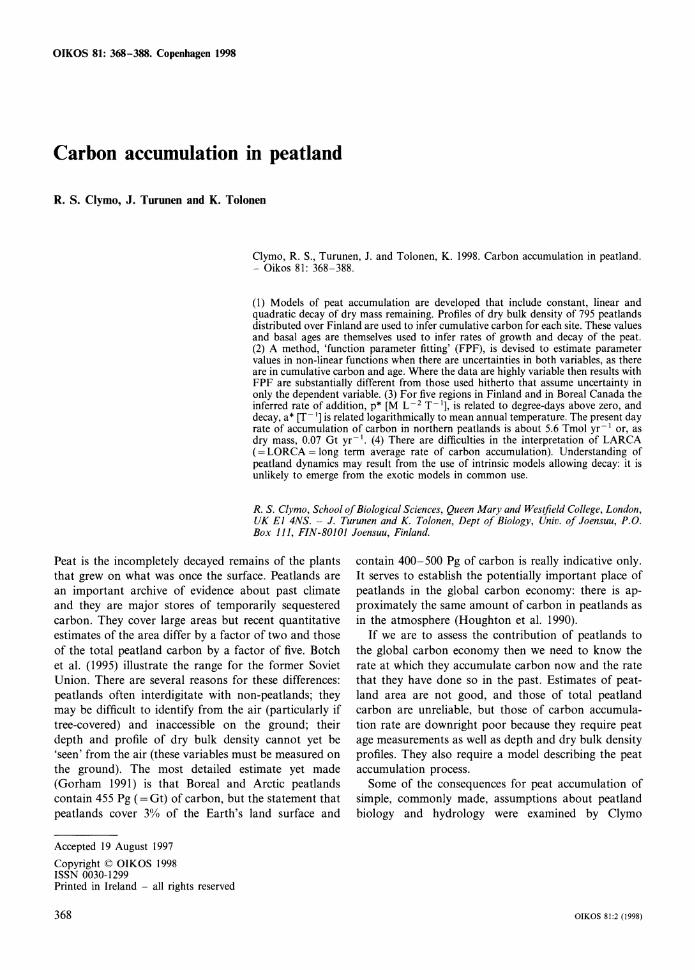
Fig. 3. Relationship of three different commonly used measures of 'peat accumulation rate'. The slope at the origin is p*, the rate at which dry matter is added to the system; the chord from the origin to the present time is LARCA = LORCA, the long term apparent rate of carbon accumulation; the slope at the present time is TRACA = ARCA, the true rate of carbon accumulation. In the inset these three rates are compared. The numerical values are always, for T > 0, in the order p* > LARCA > TRACA. It is often assumed (wrongly, if there is any decay) that p* = LARCA = TRACA.

so

= -[dr

hi^ must be solved for the particular decay rule a =

f(p) and the result rearranged to give = f(T). (2) L~~the total dry mass at time T be M,, and the

rate of addition of dry mass to the catotelm be p* [M L-2 T - 1 1. Then:

This too must be integrated for the particular decay rule. Solutions for the three decay rules of Fig. 1 are given in Table 1. Their graphs are shown in Fig. 2.

Entities and units

We have here considered dry mass but exactly the same analysis applies to carbon, except that the symbol M indicates carbon rather than dry mass, and the physical dimension M must be understood to represent the chemical mole rather than mass. The numerical factor 0.52, based on about 200 measurements, converts dry mass values to carbon, i.e. peat contains about 52%) carbon (Gorham 1991, Clymo unpubl.). This factor is larger than the 0.40 needed for carbohydrate. It is the carbon balance of peatlands that is of importance in considerations of climate change and in relation to CO, and CH,. We take the logical step of expressing the results for carbon in chemical units rather than mass ones. This makes carbon balance calculations straight- forward (carbon in peat, CO, and CH,. for example,

Age. T

can be expressed in the same units) and serves to distinguish carbon from dry mass. For example, suppose the cumulative dry mass on an area basis is 30 g cm-2 = 300 kg mP2 then the cumulative mass of carbon on an area basis is 1.3 mol = 13 kmol mP2. The same is applied to the rate of addition, p*: dry mass is shown in mass units; carbon in chemical Ones.

Basal age only

The age of the base of a peatland might be, for example, 8000 yr. If we consider this base as being T = 0 (as we have done so far) then the present surface has T = 8000 yr. Age is expressed as negative time, but as our equations use the base of the peat as datum then age is numerically identical with T. On the graphs this duality is represented by the label 'Age, T (yr)'. A S long as we use only basal dates there is no difficulty.

The accumulated mass of carbon above the base of the peat may be divided by the age of that base to give the long term apparent rate of carbon accumulation: LARCA = LORCA = M,IT [M L-2 T-'1. It corre-sponds to the slope of the chord in Fig. 3, while the rate of addition, p*, is the slope at the origin (when there is nothing to decay and so no losses). The true or actual rate of carbon accumulation now, at T, is the slope of the curve now: TRACA = ARCA = dM/dT at present. It will be obvious, and Fig. 3 shows, that for all T > 0 then p* > LARCA > TRACA. The differences among these three increase with T. Specific relations among them may be inferred from Table 1.

It is particularly important to recognise that, in the simple models considered here, in which p* and a*

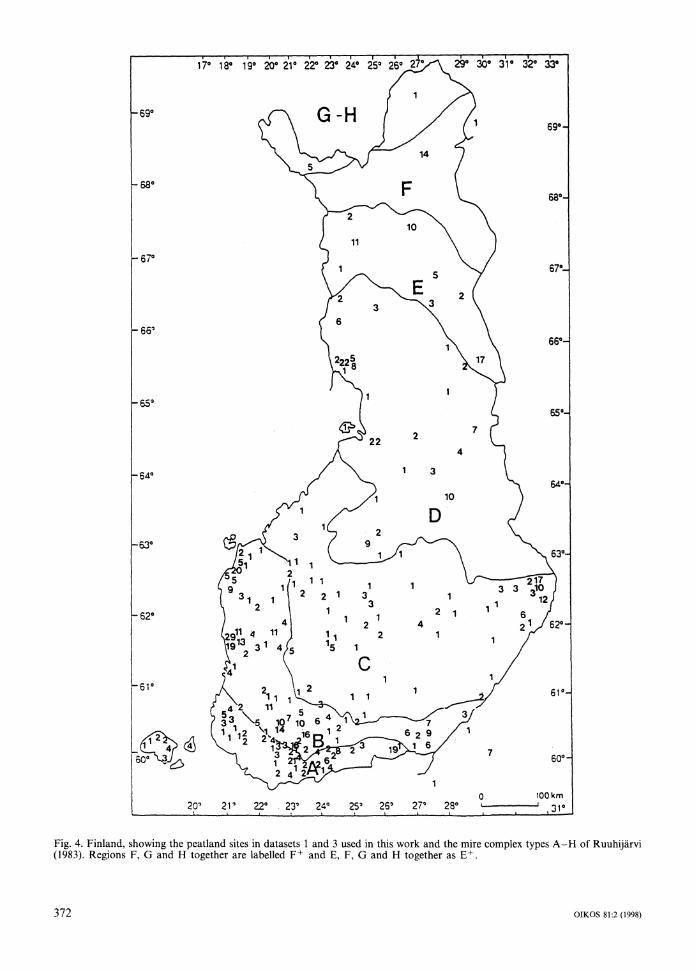
Fig. 4. Finland, showing the peatland sites in datasets 1 and 3 used in this work and the mire complex types A-H of Ruuhijarvi (1983). Regions F, G and H together are labelled F+ and E, F, G and H together as E+.

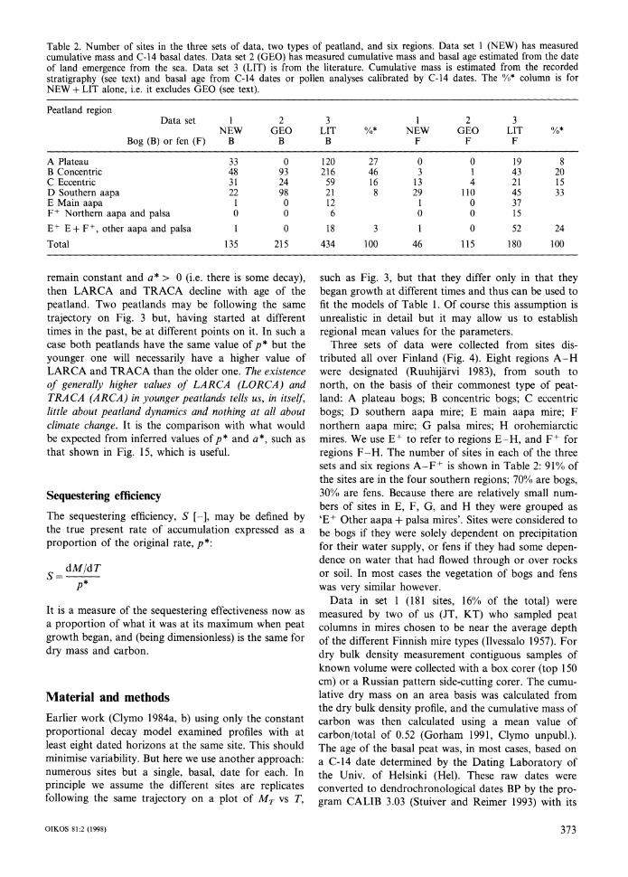
Table 2. Number of sites in the three sets of data, two types of peatland, and six regions. Data set 1 (NEW) has measured cumulative mass and C-14 basal dates. Data set 2 (GEO) has measured cumulative mass and basal age estimated from the date of land emergence from the sea. Data set 3 (LIT) is from the literature. Cumulative mass is estimated from the recorded stratigraphy (see text) and basal age from C-14 dates or pollen analyses calibrated by C-14 dates. The %* column is for NEW + LIT alone, i.e. it excludes GEO (see text).

Peatland region Data set 1 2

NEW CEO Bog (B) or fen (F) B B

A Plateau B Concentric C Eccentric D Southern aapa E Main aapa F+ Northern aapa and palsa E+ E + Ff , other aapa and palsa

Total

remain constant and a* > 0 (i.e. there is some decay), then LARCA and TRACA decline with age of the peatland. Two peatlands may be following the same trajectory on Fig. 3 but, having started at different times in the past, be at different points on it. In such a case both peatlands have the same value of p * but the younger one will necessarily have a higher value of LARCA and TRACA than the older one. The existence of generally higher ualues of LARCA (LORCA) and TRACA (ARCA) in younger peatlands tells us, in itselJ; little about peatland dynamics and nothing at all about climate change. It is the comparison with what would be expected from inferred values of p * and a*, such as that shown in Fig. 15, which is useful.

Sequestering efficiency

The sequestering efficiency, S [-I, may be defined by the true present rate of accumulation expressed as a proportion of the original rate, p*:

It is a measure of the sequestering effectiveness now as a proportion of what it was at its maximum when peat growth began, and (being dimensionless) is the same for dry mass and carbon.

Material and methods Earlier work (Clymo 1984a, b) using only the constant proportional decay model examined profiles with at least eight dated horizons at the same site. This should minimise variability. But here we use another approach: numerous sites but a single, basal, date for each. In principle we assume the different sites are replicates following the same trajectory on a plot of M , vs T ,

3 1 2 3 LIT %* NEW GEO LIT 'Xi*

B F F F

such as Fig. 3, but that they differ only in that they began growth at different times and thus can be used to fit the models of Table 1. Of course this assumption is unrealistic in detail but it may allow us to establish regional mean values for the parameters.

Three sets of data were collected from sites distributed all over Finland (Fig. 4). Eight regions A-H were designated (Ruuhijiirvi 1983), from south to north, on the basis of their commonest type of peatland: A plateau bogs; B concentric bogs; C eccentric bogs; D southern aapa mire; E main aapa mire; F northern aapa mire; G palsa mires; H orohemiarctic mires. We use E + to refer to regions E-H, and F + for regions F-H. The number of sites in each of the three sets and six regions A-F+ is shown in Table 2: 91% of the sites are in the four southern regions; 70% are bogs, 30% are fens. Because there are relatively small num- bers of sites in E, F, G, and H they were grouped as 'EtOther aapa + palsa mires'. Sites were considered to be bogs if they were solely dependent on precipitation for their water supply, or fens if they had some dependence on water that had flowed through or over rocks or soil. In most cases the vegetation of bogs and fens was very similar however.

Data in set 1 (181 sites, 16% of the total) were measured by two of us (JT, KT) who sampled peat columns in mires chosen to be near the average depth of the different Finnish mire types (Ilvessalo 1957). For dry bulk density measurement contiguous samples of known volume were collected with a box corer (top 150 cm) or a Russian pattern side-cutting corer. The cumulative dry mass on an area basis was calculated from the dry bulk density profile, and the cumulative mass of carbon was then calculated using a mean value of carbon/total of 0.52 (Gorham 1991, Clymo unpubl.). The age of the basal peat was, in most cascs, based on a C-14 date determined by the Dating Laboratory of the Univ. of Helsinki (Hel). These raw dates were converted to dendrochronological dates BP by the program CALIB 3.03 (Stuiver and Reimer 1993) with its

/ND

20-yr calibration data set and 5-point smoothing. We treat these dates as acceptably close to the true age. In a few cases the age was estimated from pollen spectra compared with C-14 dated pollen spectra from nearby sites. In a very few cases, for sites at low altitude in the region of unusually rapid land uplift around the Both- nian Bay, the independent dating of land uplift was used with the assumption that mire formation began as soon as the land emerged from the sea. A more detailed description is given by Tolonen and Turunen (1996).

Data in set 2 (330 sites, 29% of the total) were taken from peat inventory reports published by the Geologi- cal Survey of Finland during 1984-1994. They chose only peatlands more than 20 ha in extent and more than 2 m deep. Peat samples were taken with a piston corer near the centre of the peatland or near its deepest peat. The piston corer failed to produce satisfactory

Mst 0 04 P Mst 020 P I Spl 0 50 P

No/

Mst 004 P Mst 020U I Spl 0 50 P ,

Fig. 5. Simulations of carbon accumulation under the linear decay model with the rate of addition, p* = 0.0050 kmol m-2 y r - ~ ' and the decay coefficient, a t = 0.00030 y r r ' . The 48 points were first positioned randomly on the T axis and the corresponding value of M , calculated. The individual uncertainty, considered here as 'measurement error' and shown by the vertical and horizontal bars, is calculated in the three proportional (P) cases as Mst x :+ min, where Mst is a proportion (0.04 or 0.20 in the examples shown), 2 is the value on the M , or T axis, and min is a minimum: 0.2 kmol m r 2 on the M , axis and 20 yr on the Taxis. At the lower right, which is otherwise the same as the top right, the errors are uniform (U) as Mst x zmean + min. In all four graphs each point also has random Gaussian 'sample error' added to the M , and T values in proportion Spl to the exact value. In the examples shown Spl = 0.10 or 0.50. Three sorts of line are shown: T is the (true) curve for the given values of p, a* and the linear decay model. ND is the line pT, i.e. with no decay. L is the line found by 'function parameter fitting' using the median of 36 randomly chosen subsets of half the data. L, is the line fitted when all the error was assumed to be in M,.

samples in the top few dm at many sites. There is a tight linear regression between waterldry mass vs dry bulk density, so the dry bulk density in such cases was estimated from moisture content measurements. We used only those sites in the geologically young region below the highest Finnish Littorina limit. The basal age of the sites was estimated from the land uplift datings (Saarnisto 1981, Matiskainen 1989, Eronen et al. 1993, Gluckert et al. 1993) with the assumption that mire formation began as soon as the land emerged from the sea. But we made no search for the microfossils that confirm such datings (Huuikari 1956). We eliminated sites from regions above the Littorina limit because of the increasing uncertainty of such datings.

Data in set 3 (614 sites, 55% of the total) were taken from more than 30 published sources dealing with sites all over Finland (Fig. 4). A complete list of these

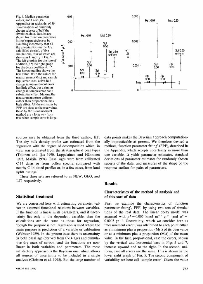
Fig. 6 . Median parameter 0 03 values, and G-ile (see Appendix) on each side, of 36 minimisations of randomly chosen subsets of half the simulated data. Results are 1shown for 'function ~arameter Msf 004

fitting' (open circlesfor by 0 02 assuming incorrectly that all the uncertainty is in the M , -A

axis (filled circles), of five r"

simulations, four of which are ! 1 1

shown as L and L, in Fig. 5. 2 The left graph is for the rate of .& addition,p*; the right graph a for the decay coefficient, a*. 0 01

The horizontal line shows the true value. With the values for measurement (Mst) and sample (Spl) error used, a five-fold change in measurement error has little effect, but a similar change in sample error has a substantial effect. Making the measurement error uniform rather than proportional has little effect. All the estimates by FPF are close to the true value; those by the usual incorrect method are a long way from true when sample error is large.

sources may be obtained from the third author, KT. The dry bulk density profile was estimated from the regression with the degree of decomposition which, in turn, was estimated from the stratigraphical peat types (Tolonen and Ijas 1990, Lappalainen and Hanninen 1993, Makila 1994). Basal ages were from calibrated C-14 dates or from pollen spectra compared with nearby C-14 dated profiles or, in a few cases, from land uplift datings.

These three sets are referred to as NEW, GEO, and LIT respectively.

Statistical treatment

We are concerned here with estimating parameter values in assumed functional relations between variables. If the function is linear in its parameters, and if uncertainty lies only in the dependent variable, then the calculations are the same as those for regression, though the purpose is not: regression is used where the main purpose is prediction of a variable or calibration (Webster 1989). In the present case there is uncertainty in both basal age (derived from C-14 age) and cumulative dry mass of carbon, and the functions are non-linear in both variables and parameters. The most satisfactory approach is the Bayesian one, which allows all sources of uncertainty to be included in a single analysis (Christen et al. 1995). But the large number of

O Oo3 I M s ~0.04 Mst 020

Ms1 020 I I I 0 002 , ,

b

2 0

SplO50 f Spl 0.50 un~form .>- umform

m

0.001 ;to ;to - I

True

data points makes the Bayesian approach computation- ally impracticable at present. We therefore devised a method, 'function parameter fitting' (FPF), described in the Appendix, which accepts uncertainty in more than one variable. It yields parameter estimates, standard deviations of parameter estimates for randomly chosen subsets of the data, and measures of the shape of the response surface for pairs of parameters.

Characteristics of the method of analysis and of this sort of data

First we examine the characteristics of 'function parameter fitting', FPF, by using two sets of simulations of the real data. The linear decay model was assumed with p* =0.005 kmol m-' yr-' and a* =

0.0003 yr-'. Uncertainty, which we consider here as 'measurement error', was attributed to each point either as a minimum plus a proportion (Mst) of its own value or as a minimum plus a proportion (Mst) of the mean value. In the first, proportional, case the errors, shown by the vertical and horizontal bars in Figs 5 and 7, increase upward and to the right. In the second, uniform, case all errors are the same. This is shown in the lower right graph of Fig. 5. The second component of variability we here call 'sample error'. Given the value

OIKOS 81.2 (1998) 375

40 ISpl 0.50

Fig. 7. Simulations similar to those of Fig. 5 (p* =0.0050 kmol m-* yr-' and a* =0.00030 yr-') with proportional measurement error (Mst = 0.05) differing only in sample error (Spl by 0.010 increments to 0.60). Two lines are shown: T is the true one (T), given the values of p*, a* and the linear decay model: L is that found by 'function parameter fitting' using the median of 36 randomly chosen subsets of half the simulated data.

True

Spl proportion Spl proport~on

Fig. 8. Median parameter values, and G-ile (see Appendix) on each side, of 36 minimisations of randomly chosed subsets of half the simulated data. Results are shown for 'function parameter fitting' (open circles) or by assuming incorrectly that all the uncertainty is in the M , axis (filled circles), for the six simulations with differing sample error shown in Fig. 7. The left graph is for the rate of addition, p*; the right graph for the decay coefficient, a*. The horizontal line shows the true value.

of T (chosen at random within specified limits of 0 and The results for four such simulations with different 11 000 yr) an exact value of M , was calculated from the values of Mst and Spl are shown in Fig. 5 , line 'L'. In linear decay model equation in Table 1. To this value Fig. 6, open circles, are shown the median parameter and to that of T was added a randomly chosen propor- values used to draw the lines in Fig. 5 (with one other tion from a Gaussian distribution with zero mean and not shown there) and their attendant G-ile (see Ap-standard deviation Spl of the mean (Spl for 'sample'). pendix). Median and G-ile are used to minimise the

376 OIKOS 81:2 (1998)

Bog NEW Bog GEO Bog LIT

;20 c- x I(

Fen NEW Fen GEO Fen LIT

Fig. 9. Depth (as cumulative carbon on an area basis, M,) vs basal age, T, for bogs (upper row) and fens (lower row) for each of the three sets of data: NEW = newly collected. GEO = from the Geological Survey of Finland, and LIT = from the literature. The symbols represent the region in Finland from south to north: A, plateau bogs =upright crosses; B, concentric bogs =diag-onal crosses: C, eccentric bogs = triangles; D. southern aapa mires = squares, Ei, other aapa and palsa mires = stars.

effects of occasional outliers. Also shown for comparison (Fig. 5 line 'Li', Fig. 6 filled circles) are the solutions by standard methods, incorrectly applied here. that assume all the uncertainty is in the M , axis alone.

The results for a second set of six simulations are shown in Figs 7 and 8. In these we explore the effects of changing Spl in more detail, with the same values of p* and a* as before, the linear decay model, and a fixed value of 0.05 (5%) proportional value of Mst.

Several conclusions may be drawn. (1) When the measurement and sample error are

small (Fig. 5 top left, compare T and L) then F P F recovers the true relationship fairly exactly. Even with substantial errors of both kinds (lower left, upper right) the agreement is still fairly close, though the fitted line, L, is always higher than and parallel to the true line. The L, lines which assume all the uncertainty is in the M , axis alone follow a different trajectory from the true line, the size of the difference being affected in the same way as that for the 'L' lines.

(2) In Fig. 6 it is clear that, for F P F (unfilled circles) and for the values of Mst and Spl chosen, a five-fold increase in Mst has a smaller effect on the exactness with which the true values of the parameters are recov- ered than does the same proportional increase in Spl. But all give values not far from the true ones. But with larger Spl and all uncertainty assumed to be in the M ,

axis the parameter values are substantially above the true ones. In effect larger values of p* are compensated by larger values of a*, causing a more rapid initial rise and later slower increase than the true one. These effects are systematic as Figs 7 and 8 show.

In short, F P F recovers the true parameter values reasonably accurately until Spl reaches about 0.60, while the incorrect method assuming all the uncertainty is in the &I, axis does not. Given the graph for Spl0.50 in Fig. 7 the similarity of the F P F line (L) and the true one (T) is really rather surprising.

One may judge from Figs 9-1 1 that in the real data the variation corresponds to Spl sO.5, and that the incorrect method overestimates p* by a factor of 2, and a* by a factor of 3-4.

Reliability of the data

The relation between cumulative carbon on an area basis (M,) and age (7')for bogs and fens in each of the three sets of data is shown in Fig. 9. There is. as one would expect, a lot of variation unrelated to mire type, area and dataset among these data. The rather sharp cutoff in age in the GEO data is a result of the decision to restrict sites to those in the geologically young region below the highest Finnish Littorina limit. The bogs in the GEO set older than 5000 yr seem to be shallower

A Plateau B Concentr~c

D Southern aapa E' Other aapa + palsa A-H All reglons

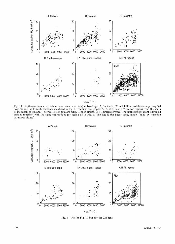
Fig. 10. Depth (as cumulative carbon on an area basis, M, ) vs basal age. T. for the NEW and LIT sets of datn comprisi~rf569 bogs among the Finnish pentlands identified in I3g. 4. The first five graphs: A, W, C, D, and E + are for regions from the south to the north of rinland. The two sets of data are NEW = open circles. LIT = upright crosses. The sixth (boxed) graph shows all regions together. with the same collventions for region as in Fig. 0. The line is the lincar decay model found by 'fi~nctioii parameter fitting'.

A Plateau B Concentrrc C Eccentrrc

5 20

2 Rl ..

10 . ** . *; * *+ . t* a, + " :+* *. 0

2.

2- + ( I * t . I f + ' * O * - *

* ' 1

8 r

D Southern aapa E' Other aapa t palsa A-H Ail regrons

Age T (YO

F I ~11 As for E ~ g .10 hut for thc 226 fell?

~ ~ o o o ~ o o o o 2 ~ ~, ~

South North 0

Bog Fen Plat Ecce Other Conc S aapa

B F P C E S a O

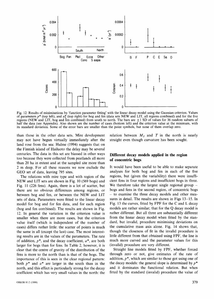
Fig. 12. Results of minimisations by 'function parameter fitting' with the linear decay model using the Gaussian criterion. Values of parameters p* (top left), and a t (top right) for bog and fen (data sets NEW and LIT, all regions combined) and for the five regions (NEW and LIT, bog and fen combined) from south to north. The bars are 1 SD of values for 36 random subsets of half the data (see Appendix). Also shown are the number of cases (bottom left) and the criterion value at the minimum, with its standard deviation. Some of the error bars are smaller than the point symbols, but none of them overlap zero.

than those in the other data sets. Mire development may not have begun virtually immediately after the land rose from the sea: Hulme (1994) suggests that on the Finnish island of Hailuoto the delay may be several centuries. The data in this set are biassed in other ways too because they were collected from peatlands all more than 20 ha in extent and at the sampled site more than 2 m deep. For all these reasons we now exclude the GEO set of data, leaving 795 sites.

The relations with mire type and with region of the NEW and LIT sets are shown in Fig. 10 (569 bogs) and Fig. l l (226 fens). Again, there is a lot of scatter, but there are no obvious differences among regions, or between bog and fen, or between the NEW and LIT sets of data. Parameters were fitted to the linear decay model for bog and for fen data, and for each region (bog and fen combined). The results are shown in Fig. 12. In general the variation in the criterion value is smaller when there are more cases, but the criterion value itself (which is independent of the number of cases) differs rather little: the scatter of points is much the same in all (except the last) case. The most interesting results are in the values of the parameters. The rate of addition, p*, and the decay coefficient, a*, are both larger for bogs than for fens. In Table 2, however, it is clear that the centre of gravity of the distribution of the fens is more to the north than is that of the bogs. The importance of this is seen in the clear regional pattern: both p* and a* are larger in the south than in the north, and this effect is particularly strong for the decay coefficient which has very small values in the north: the

relation between M , and T in the north is nearly straight even though curvature has been sought.

Different decay models applied in the region of concentric bogs

It would have been useful to be able to make separate analyses for both bog and fen in each of the five regions, but (given the variability) there were insuffi-cient fens in four regions and insufficient bogs in three. We therefore take the largest single regional group -bogs and fens in the second region, of concentric bogs - to examine the three decay models and other measures in detail. The results are shown in Figs 13-15. In Fig. 13 the curves, fitted by FPF for the C and L decay models are rather similar; that for the Q decay model is rather different. But all three are substantially different from the linear decay model when fitted by the standard, but invalid, procedure minimising deviations on the cumulative mass axis alone. Fig. 14 shows that, though the closeness of fit in the invalid procedure is little different from that obtained using FPF, the line is much more curved and the parameter values for this (invalid) procedure are very different.

Straight line models fitted by FPF, whether forced through zero or not, give estimates of the rate of addition, p*, which are similar to those got using one of the decay models: the general slope is determined by p* and it dominates the functional relation. But when fitted by the standard (invalid) procedure the value of

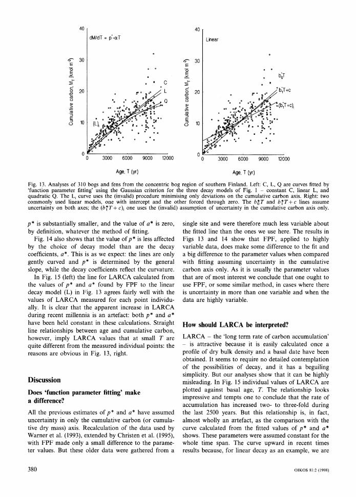
I Linear

Fig. 13. Analyses of 310 bogs and fens from the concentric bog region of southern Finland. Left: C, L, Q are curves fitted by 'function parameter fitting' using the Gaussian criterion for the three decay models of Fig. 1 constant C, linear L, and-

quadratic Q. The L, curve uses the (invalid) procedure minimising only deviations on the cumulative carbon axis. Right: two commonly used linear models, one with intercept and the other forced through zero. The hXT and b:T+ c lines assume uncertainty on both axes; the (h:T+ c), one uses the (invalid) assumption of uncertainty in the cumulative carbon axis only.

p* is substantially smaller, and the value of a* is zero, by definition, whatever the method of fitting.

Fig. 14 also shows that the value o f p * is less affected by the choice of decay model than are the decay coefficients, a*. This is as we expect: the lines are only gently curved and p* is determined by the general slope, while the decay coefficients reflect the curvature.

In Fig. 15 (left) the line for LARCA calculated from the values of p* and a* found by F P F to the linear decay model (L) in Fig. 13 agrees fairly well with the values of LARCA measured for each point individu- ally. It is clear that the apparent increase in LARCA during recent millennia is an artefact: both p* and a* have been held constant in these calculations. Straight line relationships between age and cumulative carbon, however, imply LARCA values that at small T are quite different from the measured individual points: the reasons are obvious in Fig. 13, right.

Discussion

Does 'function parameter fitting' make a difference?

All the previous estimates of p* and a* have assumed uncertainty in only the cumulative carbon (or cumulative dry mass) axis. Recalculation of the data used by Warner et al. (1993), extended by Christen et al. (1995), with F P F made only a small difference to the parameter values. But these older data were gathered from a

single site and were therefore much less variable about the fitted line than the ones we use here. The results in Figs 13 and 14 show that FPF, applied to highly variable data, does make some difference to the fit and a big difference to the parameter values when compared with fitting assuming uncertainty in the cumulative carbon axis only. As it is usually the parameter values that are of most interest we conclude that one ought to use FPF, or some similar method, in cases where there is uncertainty in more than one variable and when the data are highly variable.

How should LARCA be interpreted?

LARCA the 'long term rate of carbon accumulation' -

- is attractive because it is easily calculated once a profile of dry bulk density and a basal date have been obtained. It seems to require no detailed contemplation of the possibilities of decay, and it has a beguiling simplicity. But our analyses show that it can be highly misleading. In Fig. 15 individual values of LARCA are plotted against basal age, T. The relationship looks impressive and tempts one to conclude that the rate of accumulation has increased two- to three-fold during the last 2500 years. But this relationship is, in fact, almost wholly an artefact, as the comparison with the curve calculated from the fitted values of p* and a* shows. These parameters were assumed constant for the whole time span. The curve upward in recent times results because, for linear decay as an example, we are

Fig. 14. Left: values for the curves In Fig. 13 of rate of addit~on, p* (or b* for the straight lines). Right: values for the curves in Fig. 13 of a* (for the curved lines only: the straight ones imply no decay). The bars are II SD of values for 36 random subsets of half the data.

plotting @*/a* x In(1 + a*T)IT against T. There is a fairly strong element of ' l / T vs T' in this, so it would be surprising if the curve were not concave. The real comparison should be of the cloud of individual points with the continuous curve. That does not encourage the conclusion that there has been a recent increase in the rate of peat growth, however one defines growth.

Of course one cannot claim on this evidence that p * and a* have been shown to be nearly constant over ten millennia. But one can claim that the observations are not inconsistent with that proposition.

We do not argue that peatlands are simple systems, but that it is only after the consequences of simple assumptions have been explored and understood that one has a background against which the complexities may be investigated. For example, one approach to exploring the true dynamics of the carbon accumulation in peatlands is three dimensional reconstruction of carbon balance within the whole mire basin (Korhola et al. 1996).

Measurements of gas concentrations in peatlands (Clymo and Pearce 1995) show a profile with increasing concentrations of CO, and CH, downwards. It is difficult to account for this in any way other than as a consequence of continued decay. One may argue, therefore, that any analysis which ignores the possibility of decay is probably flawed. Our approach has been to allow the possibility and accept evidence, if it appears, that the numerical value of the decay coefficient is negligible (as it seems to be in the far north).

How do rate of addition (p*) and of decay (a*) depend on climate?

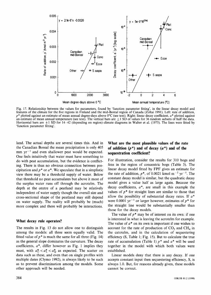
It seemed useful to seek data for peatlands in other regions and climates. Ovenden (1990) assembled data for Canada, but reports only rates of height accumulation. Zoltai (1991), however, treated C-14 date as dependent on cumulative mass for peatlands in the Boreal and Subarctic zones of Canada. We now use his Boreal data, which are sufficiently numerous, but in the oppo- site sense to give M , dependent on T, and uncertainty in both. (The data are from Zoltai's Fig. 4 graph which seems to have been swapped with that in his Fig. 2, though the captions are correct.) The C-14 dates were converted to dendrochronologically calibrated dates (equated here to age), T, and the 'Weight' to cumulative carbon, M , by the same methods as were used for the Finnish data. For illustration we present the linear decay model only, but much the same conclusions emerge if one of the other models is used. In Fig. 16 is shown the fit, and the values o f p * and a*. The value of p * is similar to that measured in the concentric bog region of Finland (Figs 13, 14) but the decay coefficient is lower: the fitted line is almost straight. Why is there a difference?

We have already noted (Fig. 12) that the values of p* and a * in Finland decrease northwards. The decay processes operate in the catotelm peat. Daily sinusoidal temperature fluctuations in a homogeneous isotropic medium (which the catotelm a roximates) are rapidly damped, and annual ones &z 19 fold less. The

Fig. 15. Left: line for LARCA = LORCA calculated for the L line and for the two valid linear regressions in Fig. 13. The points are actual values of LARCA for each site. Note that the line is not fitted to these points but calculated from the fit in the top left graph in Fig. 13. Right: sequestering ability calculated for the six lines in Fig. 13.

(annual) damping depth that depth at which the-

amplitude of the temperature wave is reduced to 1,'e =

37% of its value at the top of the catotelm - is about 1.2 m in peat (Monteith 1973, Daulat and Clymo in press). At n damping depths the amplitude is only (lle)" of the surface value. Whilst it would be wrong to claim that the peat is isothermal it is true that the temperature of most of the peat fluctuates only a few degrees around the annual mean temperature, and the deeper one goes the smaller the fluctuations. It is sensible, therefore, to look for correlations between the decay coefficient, a*, and mean annual temperature. In the field (Silvola et al. 1996: Fig. 3 back transformed to linear scale) the efflux of CO, increases linearly with average temperature, but most of this CO, is probably generated near the surface, and the average temperature hides large fluctuations. In steady laboratory condi-tions, however, the efflux of CO, and CH, is close to exponential with Celsius temperature (Daulat and Clymo in press) and the CH, at least is produced in the anoxic conditions found in the catotelm. So it seems sensible to plot the decay coefficient on a logarithmic Celsius temperature scale.

Different considerations apply to the rate of addition of carbon, p*, at the top of the acrotelm. This rate will reflect the imbalance between carbon fixation at the surface and losses, predominantly by aerobic decay, in the acrotelm. Both these processes are temperature dependent, but it is the temperature at the surface which is likely to be most important. Clymo (1984) showed that increasing the amplitude of the surface (daily) temperature wave, while keeping the mean value the same, should increase the rate of decay because, if

the temperature response is concave (as it is), a few hours at 5°C below the mean is more than compensated by the same time at 5°C above the mean. The same argument applies to carbon fixation. One might therefore look for correlations of the rate of addition, p*, with some measure of weighted integral time above 0°C.

We took climate summaries for all the stations in each of the Finnish and Canadian Boreal regions from the climate diagrams of Walter and Lieth (1975). The annual march of mean monthly temperature is approximately sinusoidal. We took the total area above zero of a sine curve centred between the reported monthly maximum and monthly minimum temperatures and offset by the mean annual temperature and used the value as an estimate of the degree-days above 0°C (DD,,). This measure has no weighting favouring higher temperatures, and it is but one of numerous similar intercorrelated indices that might have been used. But the stations were those available, and were not directly related to the peatlands either in geographical position or altitude, so we doubt if any more elaborate calculation is justifiable. A similar caveat applies to the standard deviations of the values. Fig. 18, top left, shows the relation between DD, and mean annual temperature for Finland and the area in a swathe to the south as far as the Mediterranean.

The results of comparisons o f p * and a* with climate are shown in Fig. 17. The results are remarkable, when one considers the messiness of the raw data. There is a rather clear relationship between the rate of addition, p * in all the regions (including the Canadian Boreal) and DD,. There is a near-linear relationship on a

OIKOS 81.2 (1998) 382

Fig. 16. Analysis of data collected by Zoltai (1991) from the low and mid Boreal 40 zone of Canada. Left: fitted lines for the linear decay model (Z, L) and for a straight line forced through zero (Z,bXT). Both lines were ,30 fitted by 'function parameter -E fitting'. Top right: values for the rate of addition, p* from g

2 the fitted lines, with that for 5the concentric bog region of Finland added for $ 20* comparison. Bottom right: 8 similar comparison for the linear model decay coefficient. 2 2.b;T is not shown because fit denies that there is any 0 10 decay.

0 0 3000 6000

Age. T (yr)

logarithmic scale in all the regions between the decay coefficient, a* , and mean annual temperature though the slope is too steep to be maintained at higher temperatures: a* cannot exceed 1.0, and values above 0.5 would be unlikely. The dynamics of North Ameri- can, mainly continental, peatlands and the oceanic peatlands of western Europe seem to fit into a common frame governed by peat average temperature and growing season characters.

One can explore the effects of temperature on peat accumulation in a simulation (Fig. 18). DD, increases as one moves south to higher mean annual temperatures. Within the Finnish range of DD, the increase in p* is approximately linear, but such increase cannot continue indefinitely. The highest estimates for p* are about 0.006 kmol m-' yr-', so a curve asymptotic to this value but near linear in the Finnish range of DD, is used in the simulation (Fig. 18, upper, centre). (The behaviour pattern of the whole system does not depend on the maximum value of p*, though the detail of positioning of maximum depth does depend on how rapidly the curve turns over.) A similar procedure can be used for simulating the dependence of a* on temperature. The lower part of the range, for the Finnish peatlands, gives an approximately linear relation with a* on a log scale. But one rapidly reaches a temperature at which decay has an impossibly large value. Measurements of CH, and CO, efflux in laboratory conditions (Daulat and Clymo in press) show an exponential response to Celsius temperature, with slope of 0.115"CP1. When scaled to the annual loss this gives the line in Fig. 18, top right. The curve there was used to approximate the two straight lines in the simulation.

-Cone bog '

Y ZL Zb$ Finland P a a 0002

6x10'~

Conc, bog F~nland

-? 4x10'~ z , ~ ZI -'a

2 ~ 1 0 ' ~ I9000 12000

0 -

These curves are not based on any understanding of the underlying processes: they are purely descriptive. In this they are fundamentally different from the models of peat accumulation described in the early part of this article.

The simulations in Fig. 18 are at 2000-yr intervals. All show a peak which moves t o the left (decreasing mean annual temperature) with age. These peaks result because as one moves southwards to higher temperatures both p* and a* increase, but a* does so more than p* because its relation to temperature is exponential. These graphs are not predictions: but it is interesting that - the values that result are credible and the effects (that maximum peat depth occurs in the temperature range 5-10°C) accord with experience.

What then is the r6le of water? There is empirical evidence that the depth of peat is correlated with the water supply features of climate (Granlund 1932); Clymo (1987) used Granlund's limiting curves to show that, for a given precipitation in the range 500 to 1000 mm yr-I, the limit of H2/L was constant ( H = maxi-mum depth of peat, L = diameter of peatland) and the value o f H2/L increased with precipitation. There are also theoretical reasons to exvect that the overall size and shape of rainwater-dependent peatlands will be related to the water supply (for example; Ingram 1982, Clymo 1984a, 1987) but for a given precipitation it is H2/L2 , rather than H2/L, which will be constant. Fur- ther, in the Finnish regions studied here, the same climate maps as before show that precipitation declines from a mean 644 mm yr-' in the south to 459 mm yr-' in the north. Granlund's Swedish data suggest that the maximum depth of peat to be expected in these conditions would be 30-120 cm for a 1 km-diameter peat-

CanadIan

J, m~d-Boreal Plat

* Ecce

Other +fa S aapa + S aapa

Other

Mean degree-days above 0OC Mean annual temperature (OC)

Fig. 17. Relationship between the values for parameters, found by 'function parameter fitting', in the linear decay model and features of the climate for the five regions in Finland and the mid-Boreal region of Canada (Zoltai 1991). Left: rate of addition, p* plotted against an estimate of mean annual degree-days above 0°C (see text). Right: linear decay coefficient, a* plotted against an estimate of mean annual temperature (see text). The vertical bars are 1 SD of values for 36 random subsets of half the data. Horizontal bars are i1 SD for 14-42 (depending on region) climate diagrams in Walter et al. (1975). The lines were fitted by 'function parameter fitting'.

land. The actual depths are several times this. And in the Canadian Boreal the mean precipitation is only 405 mm yr-I and even shallower peat would be expected. One feels intuitively that water must have something to do with peat accumulation, but the evidence is conflict- ing. There is thus no obvious connection between precipitation a n d p * or a*. We speculate that in a simplistic view there may be a threshold supply of water. Below that threshold no peat accumulates but above it most of the surplus water runs off through the acrotelm. The depth at the centre of a peatland may be relatively independent of water supply though the overall size and cross-sectional shape of the peatland may still depend on water supply. The reality will probably be (much) more complex and there will probably be interactions.

What decay rule operates?

The results in Fig. 13 do not allow one to distinguish among the models: all three seem equally valid. The fitted value of p* is much the same for all three (Fig. 14) as the general slope dominates the curvature. The decay coefficients, a* , differ however as Fig. 1 implies they must, with a: <a*, < a; as expected. The scatter on data such as these, and even that on single profiles with multiple dates (Clymo 1992), is always likely to be such as to prevent discrimination among the models. Some other approach will be needed.

What are the most plausible values of the rate of addition (p*) and of decay (a*) and of the sequestration coefficient?

For illustration, consider the results for 310 bogs and fens in the region of concentric bogs (Table 3). The linear decay model fitted by F P F gives an estimate for the rate of addition, p*, of 0.0021 kmol m-2 yrr l . The constant decay model is similar, but the quadratic decay model gives a value half as large again. Because the decay coefficients, a* , are small in this example the values of p* for straight lines are similar to those that allow the possibility of substantial decay rates. If a* were 0.0001 yrr l or larger however, estimates of p* for the straight line would be substantially smaller than those for the decay models.

The value of p* may be of interest on its own: if one is interested in what is leaving the acrotelm for example. The value of a* on its own is important if one wishes to account for the rate of production of CO, and CH, in the catotelm, and in the calculation of sequestering efficiency (S, Table 1; Fig. 15). But to calculate the true rate of accumulation (Table 1) p* and a* will be used together in the model with which both values were established.

Linear models deny that there is any decay. If one accepts constant input then sequestering efficiency, S, is always 1.0. But, for reasons already given, these models cannot be correct.

Mean annual temperature (OC) Mean degree-days above 0 'cU Mean annual temperature ( O C )

Mean annual temperature (O C)

Fig. 18. The consequences (lower half) for peat accumulation of combining the dependence of the parameters p* and a* on mean annual temperature. Top left shows the relation between degree-days above zero and mean annual temperature (see text). Top centre shows the relation between p* and degree-days above zero. The points and straight line are from Fig. 17. The curved line is the one used in the simulation (see text). Together these define the relation between p* and mean annual temperature. Top right is the relation between decay coefficient a* and mean annual temperature. The steep straight line is from Fig. 17; the shallower straight line is from experimental measurements (Daulat and Clymo unpubl.). The curve is that used in the simulation (see text). The lower graph combines the temperature-dependent upper graphs and the linear decay model to illustrate the course of peat accumulation at 2000-yr intervals. The lower graph is indicative only: it is not a 'prediction'.

Of the decay models one may suspect that C (con-stant decay) cannot be correct either, but beyond that we have no guidance. As a compromise therefore we take the linear model (L) as the most plausible, with p* = 0.0021 kmol mr2 yr-' and a* = 3.7 x l o r 5 yrr ' . It is interesting that a value of 0.0017 kmol m-2 y r r l was found for the net carbon sink (equivalent for p*) in coastal Alaskan wet tundra using eddy covariance methods (Vourlitis and Oechel 1997).

Fig. 15 indicates that, depending on the decay model, the sequestering efficiency. S, of long established bogs in the concentric bog region of Finland may now be only 50% to 80%. The value depends on the decay coefficient alone and not at all on the value of p*: larger values of the coefficient give smaller sequestering ability after a given time.

Most 'off-the-shelf models, of which linear regression, polynomial regression, and spline curves are examples, are exotic in the sense used by Skellam (1972). They are designed for some general situation and without consideration of the specific processes in the system being studied. Such models can (and in the case of peatlands have) lead to important miscalculations as well as failing to advance understanding of the processes at work in the peatlands.

At what rate are northern peatlands sequestering carbon?

By heroic extrapolation from these Finnish peatlands we can make an estimate for the whole Boreal and northern Subarctic region. From Table 3 we take p* =

0.0021 kmol m--' y r r l and a* = 3.7 x l o r 5 yr r ' . Ap-plying these in the equation for linear decay in Table 1 gives the rate of accumulation, dMldT, after 5000 yr ' (close to the median age) as 0.0018 kmol m-* yr (equivalent, for carbon, to about 21 g m-* yr-'; 0.21 t ha-' yr). Note that this is not the rate at which carbon is being fixed by photosynthesis: it is the present-day sequestering rate ('sink'). When converted to dry mass, and using the mean dry bulk density of 0.091 g cm-' (Makila 1994, based on 49 953 samples) we arrive at a mean depth for peatlands of 2.5 m while Gorham calculated 2.3 m. Deviations of 1 or 2 millennia make little difference to these calculations. Nor do smaller values of a* : the calculation is dominated by the value of p*.

The total area of these northern peatlands was taken by Gorham (1991) as 346 Mha (3.5 million km2; a square of side about 1900 km). Applied to our estimate of present-day sequestering rate this gives these north-

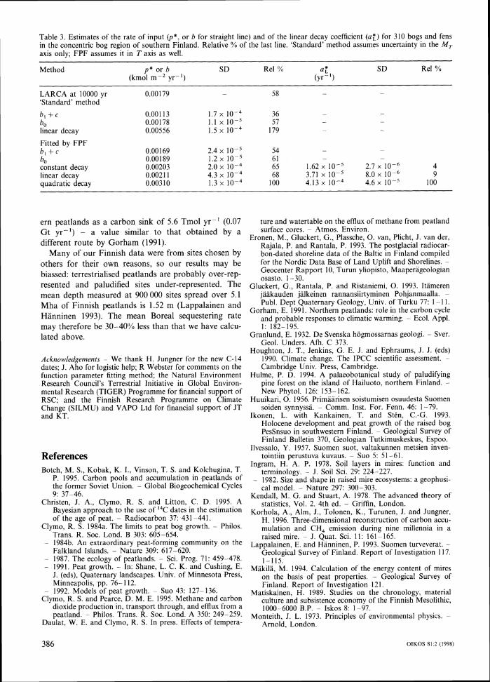
Table 3. Estimates of the rate of input (p*,or b for straight line) and of the linear decay coefficient (a*,)for 310 bogs and fens in the concentric bog region of southern Finland. Relative % of the last line. 'Standard' method assumes uncertainty in the M , axis only; F P F assumes it in T axis as well.

Method p* o r b SD (kmol m-2 yr-')

LARCA at 10000 yr 0.00179 -

'Standard' method

b, + c 0.001 13 1.7 x lo-, bo 0.00178 1.1 x l 0 v 5 linear decay 0.00556 1.5

Fitted by FPF h . + c 0.00169 2.4 x 10V5 - 1 -

6,)constant decay linear decay quadratic decay

e rn peatlands as a carbon sink of 5.6 Tmol yr-I (0.07 Gt yr-') - a value similar to that obtained by a different route by Gorham (1991).

Many of our Finnish data were from sites chosen by others for their own reasons, so our results may be biassed: terrestrialised peatlands are probably over-represented and paludified sites under-represented. The mean depth measured at 900 000 sites spread over 5.1 Mha of Finnish peatlands is 1.52 m (Lappalainen and Hanninen 1993). The mean Boreal sequestering rate may therefore be 30-40% less than that we have calculated above.

Acknowledgements We thank H. Jungner for the new C-14 -

dates; J. Aho for logistic help; R Webster for comments on the function parameter fitting method; the Natural Environment Research Council's Terrestrial Initiative in Global Environ- mental Research (TIGER) Programme for financial support of RSC; and the Finnish Research Programme on Climate Change (SILMU) and VAPO Ltd for financial support of JT and KT.

References Botch, M. S., Kobak, K. I., Vinson, T. S. and Kolchugina, 7.

P. 1995. Carbon pools and accumulation in peatlands of the former Soviet Union. Global Biogeochemical Cycles -

9: 37-46. Christen, J . A, , Clymo, R. S. and Litton. C. D. 1995. A

Bayesian approach to the use of I4C dates in the estimation of the age of peat. - Radiocarbon 37: 4 3 1 4 4 1 .

Clymo, R. S. 1984a. The limits to peat bog growth. Philos.-

Trans. R . Soc. Lond. B 303: 605-654. - 1984b. An extraordinary peat-forming community on the

Falkland Islands. Nature 309: 617-620. -

- 1987. The ecology of peatlands. - Sci. Prog. 71: 459-478. - 1991. Peat growth. - In: Shane, L. C. K. and Cushing, E.

J. (eds), Quaternary landscapes. Univ. of Minnesota Press, Minneapolis, pp. 76- 1 12.

- 1992. Models of peat growth. Suo 43: 127-136. -

Clymo, R. S, and Pearce, D. M. E. 1995. Methane and carbon dioxide production in, transport through, and efflux from a peatland. - Philos. Trans. R. Soc. Lond. A 350: 249-259.

Daulat, W. E. and Clymo, R. S. In press. Effects of tempera-

Re1 '% a*, SD Rel % (yr-')

-58 -

57 36 - -

- -

179 - -

54 -

ture and watertable on the efflux of methane from peatland surface cores. Atmos. Environ. -

Eronen, M., Gluckert, G. , Plassche, 0 . van, Plicht, J. van der, Rajala, P. and Rantala, P. 1993. The postglacial radiocarbon-dated shoreline data of the Baltic in Finland compiled for the Nordic Data Base of Land Uplift and Shorelines. -Geocenter Rapport 10, Turun yliopisto, Maaperageologian osasto. 1-30.

Gluckert, G. , Rantala, P. and Ristaniemi, 0. 1993. Itameren jaakauden jalkeinen rannansiirtyminen Pohjanmaalla. -

Publ. Dept Quaternary Geology, Univ. of Turku 77: 1-1 1. Gorham. E. 1991. Northern peatlands: role in the carbon cycle

and probable responses to climatic warming. - Ecol. Appl. I: 182-195.

Granlund, E. 1932. De Svenska hogmossarnas geologi. Sver.-

Geol. Unders. Afh. C 373. Houghton, J. T., Jenkins, G . E. J. and Ephraums, J. J. (eds)

1990. Climate change. The IPCC scientific assessment. -Cambridge Univ. Press, Cambridge.

Hulme, P. D . 1994. A palaeobotanical study of paludifying pine forest on the island of Hailuoto. northern Finland. -New Phytol. 126: 153-162.

Huuikari, 0 . 1956. Primaarisen soistumisen osuudesta Suomen soiden synnyssa. - Comm. Inst. For. Fenn. 46: 1-79.

Ikonen. L. with Kankainen, T. and Sten, C.-G. 1993. Holocene development and peat growth of the raised bog PesSnsuo in southwestern Finland. Geological Survey of -

Finland Bulletin 370, Geologian Tutkimuskeskus. Espoo. Ilvessalo. Y. 1957. Suomen suot. valtakunnen metsien inven-

tointiin perustuva kuvaus. - Suo 5: 51-61. Ingram, H. A. P. 1975. Soil layers in mires: function and

terminology. - J . Soil Sci. 29: 224-227. - 1982. Size and shape in raised mire ecosystems: a geophusi-

cal model. - Nature 297: 300-303. Kendall, M. G. and Stuart, A. 1978. The advanced theory of

statistics, Vol. 2. 4th ed. - Griffin, London. Korhola, A,, Alm, J. , Tolonen. K.. Turunen, J. and Jungner.

H. 1996. Three-dimensional reconstruction of carbon accumulation and CH, emission during nine millennia in a raised mire. - J . Quat. Sci. 11: 161 -165.

Lappalainen, E. and Hanninen, P. 1993. Suomen turveverat. -Geological Survey of Finland. Report of Investigation 1 17. 1-115.

Makila, M. 1994. Calculation of the energy content of mires on the basis of peat properties. Geological Survey of -

Finland. Report of Investigation 121. Matiskainen, H. 1989. Studies on the chronology, material

culture and subsistence economy of the Finnish Mesolithic, 1000-6000 B.P. - Iskos 8: 1-97.

Monteith. J. L. 1973. Principles of environmental physics. -Arnold, London.

Nelder. J. A. and Mead. R. 1965. A simplex method for function minimization. Computer J. 7: 308-313. -

Ovenden, L. 1990. Peat accumulation in northern wetlands. -Quat. Res. 33: 377-386.

Press. W. H., Flannery, B. P., Teukolsky, S. A. and Vetterling, W. T. 1989. Numerical recipes in PASCAL. The art of

-scientific computing. Cambridge Univ. Press, Cam-bridge.

Ruuhijirvi, R. 1983. The Finnish mire types and their regional distribution. - In: Gore. A. J. P. (ed.). Ecosystems of the World Vol4B. Mires: swamp, bog. fen and moor. Regional studies. Else~ier, Amsterdam. pp. 47-68.

Saarnisto, M. 1981. Holocene emergence history and stratigraphy in the area north of the Gulf of Bothnia. Ann. Acad. -

Sci. Fenn. AlII 130: 1-42. Silvola. J., .41m. J.. Ahlholm, U., Nykanen. H. and h4ar-

tikainen. P. J . 1996. CO2 fluxes from peat in boreal mires under varying temperature and moisture conditions. - J. Ecol. 84: 219-228.

Skellam, J. G. 1972. Some philosophical aspects of mathematical modelling in empirical science with special reference to ecology. In: Jeffers,EJ.EN.ER. (ed.), Mathematical mod- -

els in ecology. Blackwell, Oxford, pp. 13-28. Stuiver. M. and Reimer, P. J. 1993. Extended 14C database

and revised CALIB radiocarbon calibration program. -Radiocarbon 35: 215-230.

Tolonen, K . and Ijas. L. 1990. Turvessaanon arviointi suo- tyypin ja turpeen syvyyden perusteella. Suo 41: 25-32. -

- and Turunen. J . 1996. Accu~nulation rates of carbon in mires in Finland and implications for climate change. -Holocene 6: 171 - 178.

Vourlitis. G. L. and Oechel, W. C. 1997. Landscape-scale COZ, water-vapour and energy flux of moist-wet tundra ecosystems over two growing seasons. - J . Ecol. 85: 575- 590.

Walter. H. and Lieth. H. with Rehder. H. and Hatnickell, E. 3975. Klin~adiagramm-WeltAltlas. Gustav Fischer, Jena. -

Warner, B. G., Clymo, R. S. and Tolonen, K. 1993 Implica- tions of peat accumulation at Point Escuminac, New Brunswick. - Quat. Res. 39: 245 248.

Webster. R. 1989. Is regression uhat you really want? Soil-

Use Manage. 5: 47-53. Zoltai, S. C. 1991. Estimating the age of peat samples from

their weight: a study from west-central Canada. -

Holocene 1 : 68-73.

Appendix: 'function parameter fitting' with uncertainty in more than one variable

There are techniques for estimating parameter values when the function to be fitted is linear in the parameters and if there is measurement error distributed in a known manner in one of the variables only, or if the quotient of the errors in two variables is known (Kendall and Stuart 1978, Webster 1989). But the case of non-linear parameters and uncertainty of unknown distribution in more than one variable is quite common. The usual response has been that of Procrustes: to force the analysis into an existing but unsuitable mode.

Here we describe an operational solution, 'function parameter fitting' (FPF). to the more general problem of fitting an arbitrary function of one or more variables and one or more parameters. with uncertainty in more than one variable, and where the distribution in one or more of the variables is not necessarily Gaussian. The cost of this generality is that the measures of uncer-

tainty in the parameter values are not linked to the general mass of statistical theory.

Standard parameter fitting techniques in a two-variable case (y, x) minimise some function of distance on t h e y axis, in which all the uncertainty resides, between a data point and the point on the line with the same x coordinate: y -i .This puts all the weight on the y axis and none on the x axis. Here, instead of J. -2:. we use the distance normal to (at right angles to the tangent to) the fitted line, i.e, the shortest distance from the measured point to the line. This procedure requires that the scaling of the axes be specified. If the x axis were stretched enormously the procedure would approximate using y -2:. while if the J axis were stretched the procedure would approximate using .I -4.

How then should this scaling be made? We choose to use some measure of the spread of values for each variable. Each datum value is divided by the measure of spread to give the scaled value which is thus dimensionless: a necessary feature of the procedure. There are three obvious measures of spread: the standard deviation, the mean absolute deviation. and a proportion-ile such as the inter-quartile distance. For a Gaussian distribution the standard deviation is the natural choice. This is what is used in Principal Components Analysis (as well as the assumption that the relationships are linear for each variable). For a somewhat skewed distribution or one with a non-Gaussian fourth moment. and where a transformation cannot be used, the mean absolute deviation is more robust. Strongly skewed distributions or those with outliers that cannot be ignored may benefit from a proportion-ile. In prac- tice we use mean absolute de~iat ion~0.78 and the proportion-ile between 0.31 and 0.69 (the G-ile) because for a Gaussian distribution all three measures give the same value as the standard deviation. The user chooses which of these three scalings to use. but if the distribution is Gaussian it does not matter which is chosen.

The criterion we have chosen to minimise is similar to a maximum likelihood. In a space defined by all the variables with uncertainty, let c, be the shortest Eu- clidean distance from the point i to the fitted line, and e, be the error measure for the point (calculated from Euclidean combination of scaled errors on all the axes with uncertainty). Then let z = C (c, e , ) and n be the number of data points. The criterion itself in increasing order of robustness (Press et al. 1989) is then z2:2n (Gaussian), Iz 1 :n (double exponential) or (In[l + z2 /21) ln

(Cauchy, Lorentzian). We link scaling measure and criterion: standard deviation with Gaussian; standard- ised mean absolute deviation with double exponential; and G-ile with Cauchy.

It remains to specify the values of e,. They may have been measured. as in C-14 dating for example. Or they may be known to exist but not have been measured, when they must be 'guesstimated'. We use a constant proportion (of the mean) or a proportion of the datum

value. or a combination. These values of e, are used only as weights.

The whole process is incorporated in a PASCAL program. The shortest distances are found by Nelder and Mead's (1965) variable simplex method. which is not necessarily the fastest method but is robust (Press et al. 1989). Local minima are (usually) avoided by ex-panding around a tentative minimum, but there is no guarantee that the global minimum will be found. With functions of simple shape the method has proved well behaved and false global minima have been rare. The variable simplex method is used to fit the parameter values as well. Suppose the function is 'U'-shaped. As the parameter values change, the position of the 'U' may move horizontally to the right. A particular datum point may start to the right of the right limb. Its shortest distance is to the right limb and diminishes to zero, then increases until it is half way between the limbs, then transfers to the left limb. diminishes to zero. then increases indefinitely. All these changes are continuous and are automatically sensed by the method.

The process is robust but it is not easy to set inter- pretable 'confidence limits' to the parameter values. Three aids are provided however. First. a large number

of randomly chosen subsets of the data may be sub- jected to F P F and the standard deviation (or other measure if appropriate) of the parameter values gives some indication of the precision with which these values are known. Secondly, the response surface (criterion values) around pairs of parameter values, typically those locating a minimum, can be mapped in chosen detail defined by a specified proportion of the parameter value. Thirdly. for pairs of parameter values, the magnitude and direction of minimum and maximum second differences can be calculated for the same proportional change in each parameter. This allows one to assess the shape of the minimum and the extent of correlation among parameters. The behaviour of the method is illustrated in Figs 5-8.

On a 100-MHz machine the location of a minimum for two parameters. two variables each with uncer-tainty. and for 795 data points took about 5-10 min (where fitting a straight line minimising J. - J' took only 2 s). Mapping around the minimum took about 20-40 min, and getting standard deviations for 36 random subsets of half the data took about 4-8 h. These times are approximately proportional to the number of data, the number of variables, and the number of parameters.

carbon accumulation in peatland r. s. clymo; j. turunen; k...

Documents