cellular automata - federation of american scientists

by Stephen Wolfram

T t appears that the basic laws of physics relevant to everyday phenomena are now known. Yet there are manyeveryday natural systems whose complex structure and behavior have so far defied even qualitative analysis. Forexample, the laws that govern the freezing of water and the conduction of heat have long been known, butanalyzing their consequences for the intricate patterns of snowflake growth has not yet been possible. While many

complex systems may be broken down into identical components, each obeying simple laws, the huge number ofcomponents that make up the whole system act together to yield very complex behavior.

In some cases this complex behavior may be simulated numerically with just a few components. But in most casesthe simulation requires too many components, and this direct approach fails. One must instead attempt to distill

the mathematical essence of the process by which complex behavior is generated. The hope in such anapproach is to identify fundamental mathematical mechanisms that are common to many different

natural systems. Such commonality would correspond to universal features in the behavior ofvery different complex natural systems.

To discover and analyze the mathematical basis for the generation of complexity,one must identify simple mathematical systems that capture the essence of

the process. Cellular automata are a candidate class of such systems. Thisarticle surveys their nature and properties, concentrating on funda-

mental mathematical features. Cellular automata promise toprovide mathematical models for a wide variety of

complex phenomema, from turbulence in fluids topatterns in biological growth. The general

features of their behavior discussed hereshould form a basis for future

detailed studies of suchspecific systems.

The Nature of Cellular Automataand a Simple Example

Cellular automata are simple mathemati-cal idealizations of natural systems. Theyconsist of a lattice of discrete identical sites,each site taking on a finite set of, say, integervalues. The values of the sites evolve indiscrete time steps according to deterministicrules that specify the value of each site interms of the values of neighboring sites.Cellular automata may thus be considered asdiscrete idealizations of the partial differen-tial equations often used to describe naturalsystems. Their discrete nature also allows animportant analogy with digital computers:cellular automata may be viewed as parallel-processing computers of simple construction.

As a first example of a cellular automaton,consider a line of sites, each with value 0 or 1(Fig. 1). Take the value of a site at position i

for the time evolution of these site values is

(1)

where mod 2 indicates that the O or 1remainder after division by 2 is taken. Ac-

cording to this rule, the value of a particularsite is given by the sum modulo 2 (or.equivalently, the Boolean algebra “exclusiveor”) of the values of its left- and right-handnearest neighbor sites on the previous timestep. The rule is implemented simultaneouslyat each site. * Even with this very simple rulequite complicated behavior is neverthelessfound.

Fractal Patterns Grown from Cellular Au-tomata. First of all, consider evolution ac-

*In the very simplest computer implementation aseparate array of updated site values mast bemaintained and copied back CO the original sitevalue array when the updating process is com-plete.

4

1 0 1 1 0 1 0 0 0 1 1 0 1 0 1 1 0 1 0 0

Fig. 1. A typical configuration in the simple cellular automaton described by Eq. 1,consisting of a sequence of sites with values O or I. Sites with value 1 are representedby squares; those with value O are blank.

Fig. 2. A few time steps in the evolution of the simple cellular automaton defined byEq. I, starting from a “seed” containing a single nonzero site. Successive lines areobtained by successive applications of Eq. 1 at each site. According to this rule, thevalue of each site is the sum modulo 2 of the values of its two nearest neighbors on theprevious time step. The pattern obtained with this simple seed is Pascal’s triangle ofbinomial coefficients, reduced modulo 2.

Fall 1983 LOS ALAMOS SCIENCE

Cellular Automata

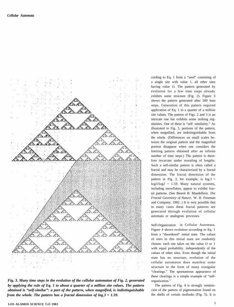
Fig. 3. Many time steps in the evolution of the cellular automaton of Fig. 2, generatedby applying the rule of Eq. 1 to about a quarter of a million site values. The patternobtained is “self-similar”: a part of the pattern, when magnified, is indistinguishablefrom the whole. The pattern has a fractal dimension of log23 = 1.59.

LOS ALAMOS SCIENCE Fall 1983

cording to Eq. 1 from a “seed” consisting ofa single site with value 1, all other siteshaving value O. The pattern generated byevolution for a few time steps alreadyexhibits some structure (Fig. 2). Figure 3shows the pattern generated after 500 timesteps. Generation of this pattern requiredapplication of Eq. 1 to a quarter of a millionsite values. The pattern of Figs. 2 and 3 is anintricate one but exhibits some striking reg-ularities. One of these is “self -similarity.” Asillustrated in Fig. 3, portions of the pattern,when magnified, are indistinguishable from

the whole. (Differences on small scales be-tween the original pattern and the magnifiedportion disappear when one considers thelimiting pattern obtained after an infinitenumber of time steps.) The pattern is there-fore invariant under resealing of lengths.Such a self-similar pattern is often called afractal and may be characterized by a fractaldimension. The fractal dimension of thepattern in Fig. 3, for example, is logz3 =log3/log2 = 1.59. Many natural systems,including snowflakes, appear to exhibit frac-tal patterns. (See Benoit B. Mandelbrot, TheFractal Geornetry of Nature, W. H. Freemanand Company, 1982. ) It is very possible thatin many cases these fractal patterns aregenerated through evolution of cellularautomata or analogous processes.

Self-Organization in Cellular Automata.

Figure 4 shows evolution according to Eq. 1from a “disordered” initial state. The valuesof sites in this initial state are randomlychosen: each site takes on the value O or 1with equal probability. independently of thevalues of other sites. Even though the initialstate has no structure, evolution of thecellular automaton does manifest somestructure in the form of many triangular“clearings.” The spontaneous appearance ofthese clearings is a simple example of “self-organization.”

The pattern of Fig. 4 is strongly reminis-cent of the pattern of pigmentation found onthe shells of certain mollusks (Fig. 5). It is

5

quite possible that the growth of thesepigmentation patterns follows cellular au-tomaton rules.

In systems that follow conventionalthermodynamics, the second law ofthermodynamics implies a progressive deg-radation of any initial structure and a univer-sal tendency to evolve with time to states ofmaximum entropy and maximum disorder.While many natural systems do tend towarddisorder, a large class of systems, biologicalones being prime examples, show a reversetrend: they spontaneously generate structurewith time, even when starting from dis-ordered or structureless initial states. Thecellular automaton in Fig. 4 is a simpleexample of such a self-organizing system.The mathematical basis of this behavior isrevealed by considering global properties ofthe cellular automaton. Instead of followingevolution from a particular initial state, as inFig. 4, one follows the overall evolution of anensemble of many different initial states.

It is convenient when investigating globalproperties to consider finite cellular autom-ata that contain a finite number N of siteswhose values are subject to periodic bound-

ary conditions. Such a finite cellular automa-ton may be represented as sites arranged, forexample. around a circle. If each site has twopossible values, as it does for the rule of Eq.1, there are a total of 2 n possible states, orconfigurations, for the complete finite cellu-lar automaton. The global evolution of thecellular automaton may then be represented

by a finite state transition graph plotted inthe “state space” of the cellular automaton.Each of the 2 n possible states of the com-plete cellular automaton (such as the state110101101010 for a cellular automaton withtwelve sites) is represented by a node, orpoint, in the graph, and a directed lineconnects each node to the node generated bya single application of the cellular automatonrule. The trajectory traced out in state spaceby tbe directed lines connecting oneparticular node to its successors thus cor-responds to the time evolution of the cellular

6

Fig. 4. Evolution of the simple cellular automaton defined by Eq. I, from a disorderedinitial state in which each site is taken to have value O or 1 with equal, independentprobabilities. Evolution of the cellular automaton even from such a random initialstate yields some simple structure.

Fig. 5. A “cone shell” with a pigmentation pattern reminiscent of the pattern generatedby the cellular automaton of Fig. 4. (Shell courtesy of P. Hut.)


Cellular Automata

automaton from the initial state representedby that particular node. The state transitiongraph of Fig. 6 shows all possible trajectoriesin state space for a cellular automaton withtwelve sites evolving according to the simplerule of Eq. 1.

A notable feature of Fig. 6 is the presence

of trajectories that merge with time. Whileeach state has a unique successor in time, itmay have several predecessors or no pred-ecessors at all (as for states on the periphery


Fig. 6. The global state transition graphfor a finite cellular automaton consistingof twelve sites arranged around a circleand evolving according to the simple ruleof Eq. 1. Each node in the graph repre-sents one of the 4096 possible states, orsequences of the twelve site values, of thecellular automaton. Each node is joinedby a directed line to a successor nodethat corresponds to the state obtained byone time step of cellular automatonevolution. The state transition graphconsists of many disconnected pieces,many of identical structure. Only onecopy of each structurally identical pieceis shown explicitly. Possible pathsthrough the state transition graph rep-resent possible trajectories in the statespace of the cellular automaton. Themerging of these trajectories reflects theirreversibility of the cellular automatonevolution. Any initial state of thiscellular automaton ultimately evolves toan “attractor” represented in the graphby a cycle. For this particular cellularautomaton all configurations evolve toattractors in at most three time steps.(From O. Martin, A. Odlyzko, and S.Wolfram, “Algebraic Properties ofCellular Automata, ” Bell Laboratoriesreport (January 1983) and to be pub-lished in Communications in Mathemat-ical Physics.)

of the state transition graph). The merging oftrajectories implies that information is lost inthe evolution of the cellular automaton:knowledge of the state attained by the sys-tem at a particular time is not sufficient todetermine its history uniquely, so that theevolution is irreversible. Starting with aninitial ensemble in which all configurationsoccur with any distribution of probabilities.the irreversible evolution decreases theprobabilities for some configurations and

increases those for others. For example, afterjust one time step the probabilities for stateson the periphery of the state transition graphin Fig. 6 are reduced to zero; such statesmay be given as initial conditions, but maynever be generated through evolution of thecellular automaton. After many time stepsonly a small number of all the possibleconfigurations actually occur. Those that dooccur may be considered to lie on “attrac-tors” of the cellular automaton evolution.Moreover. if the attractor states have special

“organized” features, these features will ap-pear spontaneously in the evolution of thecellular automaton. The possibility of self-organization is therefore a consequence ofthe irreversibility of the cellular automatonevolution, and the structures obtainedthrough self-organization are determined bythe characteristics of the attractors.

The irreversibility of cellular automatonevolution revealed by Fig, 6 is to be con-trasted with the intrinsic reversibility of sys-tems described by conventional thermo-dynamics. At a microscopic level the trajec-tories representing the evolution of states insuch systems never merge: each state has aunique predecessor. and no information islost with time, Hence a completely dis-ordered ensemble, in which all possible statesoccur with equal probabilities, remains dis-ordered forever. Moreover. if nearby statesarc grouped (or “coarse-grained”) together.as by imprecise measurements, then withtime the probabilities for different groups ofstates will tend to equality. regardless of theirinitial values. In this way such systems tendwith time to complete disorder and max-imum entropy. as prescribed by the secondlaw of thermodynamics. Tendency to dis-order and increasing entropy are universalfeatures of intrinsically reversible systems instatistical mechanics. Irreversible systems,such as the cellular automaton of Figs. 2, 3,and 4, counter this trend, but universal lawshave yet to be found for their behavior andfor the structures they may generate. Onehopes that such general laws may ultimately

7

be abstracted from an investigation of thecomparatively simple examples provided bycellular automata.

While there is every evidence that thefundamental microscopic laws of physics areintrinsically reversible (information-preserv-ing, though not precisely time-reversal in-variant), many systems behave irreversiblyon a macroscopic scale and are ap-propriately described by irreversible laws,For example, while the microscopic molecu-lar interactions in a fluid are entirely re-versible, macroscopic descriptions of theaverage velocity field in the fluid, using, say,the Navier-Stokes equations, are irreversibleand contain dissipative terms. Cellular au-tomata provide mathematical models at thismacroscopic level.

Mathematical Analysis of a SimpleCellular Automaton

The cellular automaton rule of Eq. 1 isparticularly simple and admits a rather com-plete mathematical analysis.

The fractal patterns of Figs. 2 and 3 maybe characterized in a simple algebraic man-ner. If no reduction modulo 2 were per-formed, then the values of sites generatedfrom a single nonzero initial site wouldsimply be the integers appearing in Pascal’striangle of binomial coefficients. The patternof nonzero sites in Figs. 2 and 3 is thereforethe pattern of odd binomial coefficients inPascal’s triangle. (See Stephen Wolfram,“Geometry of Binomial Coefficients,” to bepublished in American MathematicalMonthly.)

This algebraic approach may be extendedto determine the structure of the state tran-sition diagram of Fig. 6. (See O. Martin, A.Odlyzko, and S. Wolfram, “AlgebraicProperties of Cellular Automata,” Bell Labo-ratories report (January 1983) and to bepublished in Communications in Mathemati-cal Physics,) The analysis proceeds by writ-

ing for each configuration a characteristicpolynomial

where x is a dummy variable, and thecoefficient of xi is the value of the site atposition i. In terms of characteristic poly-nomials, the cellular automaton rule of Eq. 1takes on the particularly simple form

where

T(x) = (x + x-’)

and all arithmetic on the polynomial coeffi-cients is performed modulo 2. The reductionmodulo xN –1 implements periodic boundaryconditions. The structure of the state tran-sition diagram may then be deduced fromalgebraic properties of the polynomial T(x).For even N one finds, for example, that thefraction of states on attractors is 2-D2(N) ,where D2(N) is defined as the largest integralpower of 2 that divides N (for example,D2(12) = 4).

Since a finite cellular automaton evolvesdeterministically with a finite total number ofpossible states, it must ultimately enter acycle in which it visits a sequence of statesrepeatedly. Such cycles are manifest asclosed loops in the state transition graph.The algebraic analysis of Martin et al. showsthat for the cellular automaton of Eq. 1 themaximal cycle length II (of which all othercycle lengths are divisors) is given for even Nby

or

and in fact is almost always equal to thisvalue (the first exception occurs for N = 37),Here sord N (2) is a number theoretical func-tion defined to be the minimum positive

maximum value of sord N (2), typicallyachieved when N is prime, is (N–1)/2. Themaximal cycle length is thus of order 2N/2,approximately the square root of the totalnumber of possible states 2N.

An unusual feature of this analysis is theappearance of number theoretical concepts.Number theory is inundated with complexresults based on very simple premises. Itmay be part of the mathematical mechanismby which natural systems of simple construc-tion yield complex behavior,

More General Cellular Automata

The discussion so far has concentrated onthe particular cellular automaton rule givenby Eq. 1. This rule may be generalized inseveral ways. One family of rules is obtainedby allowing the value of a site to be anarbitrary function of the values of the siteitself and of its two nearest neighbors on theprevious time step:

A convenient notation illustrated in Fig. 7.assigns a “rule number” to each of the 256rules of this type. The rule number of Eq. 1 is90 in this notation.

Further generalizations allow each site ina cellular automaton to take on an arbitrary

8 Fall 1983 LOS ALAMOS SCIENCE

Cellular Automata

Universality Classes in CellularAutomata

Fig. 7. Assignment of rule numbers to cellular automata for which k = 2 andr = I. The values of sites obtained from each of the eight possible three-siteneighborhoods are combined to form a binary number that is quoted as a decimalinteger. The example shown is for the rule given by Eq. 1.

number k of values and allow the value of asite to depend on the values of sites at adistance up to r on both sides. so that

The number of different rules with given kand r grows as kk2r+1 and therefore becomesimmense even for rather small k and r.

Figure 8 shows examples of evolutionaccording to some typical rules with variousk and r values. Each rule leads to patternsthat differ in detail. However, the examplessuggest a very remarkable result: all patternsappear to fall into only four qualitativeclasses. These basic classes of behavior maybe characterized empirically as follows:

. Class l—evolution leads to a homogene-

ous state in which, for example, all sites havevalue O;

stable or periodic structures that are sepa-


rated and simple;

pattern;Class 4—evolution leads to complex

structures, sometimes long-lived.

Examples of these classes are indicated inFig. 8.

The existence of only four qualitativeclasses implies considerable universality inthe behavior of cellular automata; manyfeatures of cellular automata depend only onthe class in which they lie and not on theprecise details of their evolution. Such uni-versality is analogous, though probably notmathematically related, to the universalityfound in the equilibrium statistical mechanicsof critical phenomena. In that case manysystems with quite different detailed con-struction are found to lie in classes withcritical exponents that depend only on gen-eral, primarily geometrical features of thesystems and not on their detailed construc-tion.

To proceed in analyzing universality incellular automata, one must first give morequantitative definitions of the classes identi-fied above. One approach to such definitionsis to consider the degree of predictability ofthe outcome of cellular automaton evolution,given knowledge of the initial state. For class1 cellular automata complete prediction istrivial: regardless of the initial state, thesystem always evolves to a unique homoge-neous state. Class 2 cellular automata havethe feature that the effects of particular sitevalues propagate only a finite distance, thatis, only to a finite number of neighboringsites. Thus a change in the value of a singleinitial site affects only a finite region of sitesaround it, even after an infinite number oftime steps. This behavior, illustrated in Fig.9, implies that prediction of a particular finalsite value requires knowledge of only a finiteset of initial site values. In contrast, changesof initial site values in class 3 cellular autom-ata, again as illustrated in Fig. 9, almostalways propagate at a finite speed foreverand therefore affect more and more distantsites as time goes on. The value of aparticular site after many time steps thusdepends on an ever-increasing number ofinitial site values. If the initial state is dis-ordered, this dependence may lead to anapparently chaotic succession of values for aparticular site. In class 3 cellular automata,therefore, prediction of the value of a site atinfinite time would require knowledge of aninfinite number of initial site values. Class 4cellular automata are distinguished by aneven greater degree of unpredictability, asdiscussed below.

Class 2 cellular automata may be con-sidered as “filters” that select particularfeatures of the initial state. For example, aclass 2 cellular automata may be constructedin which initial sequences 111 survive, butsites not in such sequences eventually attain

9

Fig. 9. Difference patterns showing the differences between the rule: for class 2 rules the effects have finite range; for classconfigurations generated by evolution, according to various 3 rules the effects propagate to neighboring sites indefinitely atcellular automaton rules, from initial states that differ in the a fixed speed; and for class 4 rules the effects also propagatevalue of a single site. Each difference pattern is labeled by the to neighboring sites indefinitely but at various speeds. Thebehavior class of the cellular automaton rule. The effects of difference patterns shown here are analogues of Green’schanges in a single site value depend on the behavior class of functions for cellular automata.

value O. Such cellular automata are of prac-tical importance for digital image processing:they may be used to select and enhanceparticular patterns of pixels. After a suffi-ciently long time any class 2 cellular automa-ton evolves to a state consisting of blockscontaining nonzero sites separated by re-gions of zero sites. The blocks have a simpleform. typically consisting of repetitions ofparticular site values or sequences of sitevalues (such as 101010. . .). The blockseither do not change with time (yieldingvertical stripes in the patterns of Fig. 8) orcycle between a few states (yielding “railroadtrack” patterns).

While class 2 cellular automata evolve togive persistent structures with small periods,class 3 cellular automata exhibit chaoticaperiodic behavior, as shown in Fig. 8.Although chaotic, the patterns generated byclass 3 cellular automata are not completely

random. In fact, as mentioned for the exam-ple of Eq. 1, they may exhibit important self-organizing behavior. In addition and again incontrast to class 2 cellular automata, thestatistical properties of the states generatedby many time steps of class 3 cellularautomaton evolution are the same for almostall possible initial states. The large-timebehavior of a class 3 cellular automaton istherefore determined by these commonstatistical properties.

The configurations of an infinite cellularautomaton consist of an infinite sequence ofsite values. These site values could be con-sidered as digits in a real number, so thateach complete configuration would cor-respond to a single real number. The topol-ogy of the real numbers is. however, notexactly the same as the natural one for theconf igura t ions ( the b inary numbers0.111111 . . . and 1.00000 . . . are identical,

but the corresponding configurations arenot). Instead. the configurations of an infinitecellular automaton form a Cantor set. Figure10 illustrates two constructions for a Cantorset. In construction (a) of Fig. 10. one startswith the set of real numbers in the interval Oto 1. First one excludes the middle third ofthe interval, then the middle third of eachinterval remaining, and so on. In the limit theset consists of an infinite number of discon-nected points. If positions in the interval arerepresented by ternimals (base 3 fractions,analogous to base 10 decimals). then theconstruction is seen to retain only pointswhose positions are represented by ternimalscontaining no 1‘s (the point 0.2202022 istherefore included; 0.2201022 is excluded).An important feature of the limiting set is its

self-similarity. or fractal form: a piece of theset, when magnified, is indistinguishablefrom the whole. This self-similarity is math-


emetically analogous to that found for thelimiting two-dimensional pattern of Fig. 3.

In construction (b) of Fig. 10, the Cantorset is formed from the “leaves” of an infinitebinary tree. Each point in the set is reachedby a unique path from the “root” (top asdrawn) of the tree. This path is specified byan infinite sequence of binary digits, in whichsuccessive digits determine whether the left-or right-hand branch is taken at each suc-cessive level in the tree. Each point in theCantor set corresponds uniquely to oneinfinite sequence of digits and thus to oneconfiguration of an infinite cellular automa-ton. Evolution of the cellular automaton thencorresponds to iterated mappings of theCantor set to itself. (The locality of cellularautomaton rules implies that the mappingsare continuous.) This interpretation of cellu-lar automata leads to analogies with thetheory of iterated mappings of intervals ofthe real line. (See Mitchell J. Feigenbaum,“Universal Behavior in Nonlinear Systems,”Los Alamos Science, Vol. 1, No. 1(1980):4-27.)

Cantor sets are parameterized by their“dimensions.” A convenient definition ofdimension, based on construction (a) of Fig.10, is as follows, Divide the interval from 0to 1 into k17 bins, each of width k n. Then letN(n) be the number of these bins thatcontain points in the set. For large n thisnumber behaves according to

N(n) - kd” . (2)

and d is defined as the “set dimension” of theCantor set. If a set contained all points in theinterval O to 1, then with this definition itsdimension would simply be 1. Similarly, anyfinite number of segments of the real linewould form a set with dimension 1. How-ever, the Cantor set of construction (a’),which contains an infinite number of discon-nected pieces, has a dimension according to

An alternative definition of dimension,agreeing with the previous one for present

14

0 2

0 0 2

0 2

(b)

Fig. 10. Steps in two constructions of a Cantor set. At each step in construction (a),the middle third of all intervals is excluded. The first step thus excludes all pointswhose positions, when expressed as base 3 fractions, have a 1 in the first “ternimalplace” (by analogy with decimal place), the second step excludes all points whosepositions have a 1 in the second ternimal place, and so on. The limiting set obtainedafter an infinite number of steps consists of an infinite number of disconnected pointswhose positions contain no 1‘s. The set maybe assigned a dimension, according to Eq.

Cantor set. Infinite sequences of digits, representing cellular automaton configura-tions, are seen to correspond uniquely with points in the Cantor set.


Cellular Automata

Fig. 11. Time evolution of the probabilities for each of the 1024 possible configura-tions of a typical class 3 cellular automaton with k = 2 and r = I and of size 10,starting from an initial ensemble in which each possible configuration occurs withequal probability. The configurations are specified by integers whose binary digitsform the sequence of site values. The probability for a particular configuration is givenon successive lines in a vertical column: a dot appears at a particular time step if theconfiguration occurs with nonzero probability at that time step. In the initial ensembleall configurations occur with equal nonzero probabilities, and dots appear in allpositions. The cellular automaton evolution modifies the probabilities for theconfigurations, making some occur with zero probability and yielding gaps in whichno dots appear. This “thinning” is a consequence of the irreversibility of the cellularautomaton evolution and is reflected in a decrease of entropy with time. In the limit ofcellular automata of infinite size, the configurations appearing at large times form aCantor set. For the rule shown (rule 18 in the notation of Fig. 7) the limitingdimension of this Cantor set is found to be approximately 0.88.

purposes. is based on self-similarity. Takethe Cantor set of construction (a) in Fig. 10.Contract the set by a magnification factork-m. By virtue of its self-similarity, the wholeset is identical to a number, say M(m), o fcopies of this contracted copy. For large m,

set dimension.With these definitions the dimension of the

Cantor set of all possible configurations foran infinite one-dimensional cellular automa-ton is 1. A disordered ensemble. in whicheach possible configuration occurs withequal probability, thus has dimension I.Figure 11 shows the behavior of theprobabilities for the configurations of a typi-cal cellular automaton as a function of time.


starting from such a disordered initialensemble, As expected from the irre-versibility of cellular automaton evolution,exemplified by the state transition graph ofFig. 6, different configurations attain dif-ferent probabilities as evolution proceeds.and the probabilities for some configurationsdecrease to zero. This phenomenon is mani-fest in the “thinning” of configurations onsuccessive time steps apparent in Fig. I I.The set of configurations that survive withnonzero probabilities after many time stepsof cellular automaton evolution constitutesthe “attractors” for the evolution. This set isagain a Cantor set; for the example of Fig.

1.755 is the real solution of the polynomial

equation z3 – Z2 + 2 Z – 1 = 0. (See D. A.

Lind, “Applications of Ergodic Theory andSofic Systems to Cellular Automata.” Uni-versity of Washington preprint (April 1983)and to be published in Physica D; see alsoMartin et al., op. cit.) The greater theirreversibility in the cellular automaton evo-lution, the smaller is the dimension of theCantor set corresponding to the attractorsfor the evolution. If the set of attractors for acellular automaton has dimension 1, thenessentially all the configurations of thecellular automaton may occur at large times.If the attractor set has dimension less than 1.then a vanishingly small fraction of allpossible configurations are generated aftermany time steps of evolution. The attractorsets for most class 3 cellular automata havedimensions less than 1. For those class 3cellular automata that generate regular pat-terns, the more regular the pattern, thesmaller is the dimension of the attractor set;these cellular automata are more irreversibleand are therefore capable of a higher degreeof self-organization.

The dimension of a set of cellular automa-ton configurations is directly proportional tothe limiting entropy (or information) per siteof the sequence of site values that make upthe configurations. (See Patrick Billingsley,Ergodic Theory and Information, JohnWiley & Sons. 1965.) If the dimension of theset was 1, so that all possible sequences ofsite values could occur, then the entropy ofthese sequences would be maximal. Di-mensions lower than 1 correspond to sets inwhich some sequences of site values areabsent, so that the entropy is reduced. Thusthe dimension of the attractor for a cellularautomaton is directly related to the limitingentropy attained in its evolution, startingfrom a disordered ensemble of initial states.

Dimension gives only a very coarsemeasure of the structure of the set of con-figurations reached at large times in a

cellular automaton. Formal language theorymay provide a more complete characteriza-tion of the set. “Languages” consist of a set

15

of words, typically infinite in number.

formed from a sequence of letters accordingto certain grammatical rules. Cellular

automaton configurations are analogous towords in a formal language whose letters arethe k possible values of each cellular automa-ton site. A grammar then gives a succinctspecification for a set of cellular automatonconfigurations.

Languages may be classified according tothe complexity of the machines or computersnecessary to generate them. A simple classof languages specified by “regular gram-mars’” may be generated by finite statemachines. A finite state machine is repre-sented by a state transition graph (analogousto the state transition graph for a finitecellular automaton illustrated in Fig. 6). Thepossible words in a regular grammar aregenerated by traversing all possible paths inthe state transition graph. These words maybe specified by “regular expressions” consist-ing of finite length sequences and arbitraryrepetitions of these, For example, the regularexpression 1(00)* 1 represents all sequencescontaining an even number of O’s (arbitraryrepetition of the sequence 00) flanked by apair of 1’s. The set of configurations ob-tained at large times in class 2 cellularautomata is found to form a regular lan-guage. It is likely that attractors for otherclasses of cellular automata correspond tomore complicated languages.

Analogy with DynamicalSystems Theory

The three classes of cellular automatonbehavior discussed so far are analogous tothree classes of behavior found in the solu-tions to differential equations (continuousdynamical systems). For some differentialequations the solutions obtained with anyinitial conditions approach a fixed point atlarge times. This behavior is analogous toclass 1 cellular automaton behavior. in asecond class of differential equations, thelimiting solution at large times is a cycle inwhich the parameters vary periodically withtime. These equations are analogous to class2 cellular automata. Finally. some differen-tial equations have been found to exhibitcomplicated, apparently chaotic behavior de-pending in detail on their initial conditions.With the initial conditions specified by deci-mals, the solutions to these differential equa-tions depend on progressively higher andhigher order digits in the initial conditions.This phenomenon is analogous to the de-pendence of a particular site value on pro-

16

Evolution of a class 4 cellular automaton from several disordered initial

states. The bottom example has been reproduced on a larger scale to show detail. Inthis cellular automaton, for which k = 2 and r = 2, the value of a site is 1 only if a totalof two or four sites out of the five in its neighborhood have the value 1 on the previoustime step. For some initial states persistent structures are formed, some of whichpropagate with time. This cellular automaton is believed to support universalcomputation, so that with suitable initial states it may implement any finite algorithm.


Cellular Automata

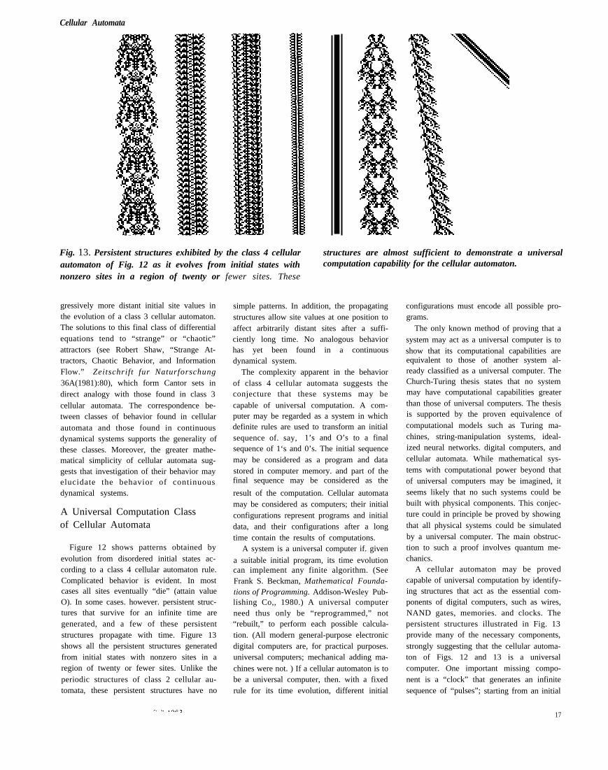
Fig. 13. Persistent structures exhibited by the class 4 cellularautomaton of Fig. 12 as it evolves from initial states withnonzero sites in a region of twenty or fewer sites. These

structures are almost sufficient to demonstrate a universalcomputation capability for the cellular automaton.

gressively more distant initial site values inthe evolution of a class 3 cellular automaton.The solutions to this final class of differentialequations tend to “strange” or “chaotic”attractors (see Robert Shaw, “Strange At-tractors, Chaotic Behavior, and InformationFlow.” Zeitschrift fur Naturforschung36A(1981):80), which form Cantor sets indirect analogy with those found in class 3cellular automata. The correspondence be-tween classes of behavior found in cellularautomata and those found in continuousdynamical systems supports the generality ofthese classes. Moreover, the greater mathe-matical simplicity of cellular automata sug-gests that investigation of their behavior mayelucidate the behavior of continuousdynamical systems.

A Universal Computation Classof Cellular Automata

Figure 12 shows patterns obtained byevolution from disordered initial states ac-cording to a class 4 cellular automaton rule.Complicated behavior is evident. In mostcases all sites eventually “die” (attain valueO). In some cases. however. persistent struc-tures that survive for an infinite time aregenerated, and a few of these persistentstructures propagate with time. Figure 13shows all the persistent structures generatedfrom initial states with nonzero sites in aregion of twenty or fewer sites. Unlike theperiodic structures of class 2 cellular au-tomata, these persistent structures have no

simple patterns. In addition, the propagatingstructures allow site values at one position toaffect arbitrarily distant sites after a suffi-ciently long time. No analogous behaviorhas yet been found in a continuousdynamical system.

The complexity apparent in the behaviorof class 4 cellular automata suggests theconjecture that these systems may becapable of universal computation. A com-puter may be regarded as a system in whichdefinite rules are used to transform an initialsequence of. say, 1’s and O’s to a finalsequence of 1‘s and 0’s. The initial sequencemay be considered as a program and datastored in computer memory. and part of thefinal sequence may be considered as the

result of the computation. Cellular automatamay be considered as computers; their initialconfigurations represent programs and initialdata, and their configurations after a longtime contain the results of computations.

A system is a universal computer if. given

a suitable initial program, its time evolutioncan implement any finite algorithm. (SeeFrank S. Beckman, Mathematical Founda-tions of Programming. Addison-Wesley Pub-lishing Co,, 1980.) A universal computerneed thus only be “reprogrammed,” not“rebuilt,” to perform each possible calcula-tion. (All modern general-purpose electronicdigital computers are, for practical purposes.universal computers; mechanical adding ma-chines were not. ) If a cellular automaton is tobe a universal computer, then. with a fixedrule for its time evolution, different initial

configurations must encode all possible pro-grams.

The only known method of proving that asystem may act as a universal computer is toshow that its computational capabilities areequivalent to those of another system al-ready classified as a universal computer. TheChurch-Turing thesis states that no systemmay have computational capabilities greaterthan those of universal computers. The thesisis supported by the proven equivalence ofcomputational models such as Turing ma-chines, string-manipulation systems, ideal-ized neural networks. digital computers, andcellular automata. While mathematical sys-tems with computational power beyond thatof universal computers may be imagined, itseems likely that no such systems could bebuilt with physical components. This conjec-ture could in principle be proved by showingthat all physical systems could be simulatedby a universal computer. The main obstruc-tion to such a proof involves quantum me-chanics.

A cellular automaton may be provedcapable of universal computation by identify-ing structures that act as the essential com-ponents of digital computers, such as wires,NAND gates, memories. and clocks. Thepersistent structures illustrated in Fig. 13provide many of the necessary components,strongly suggesting that the cellular automa-ton of Figs. 12 and 13 is a universalcomputer. One important missing compo-nent is a “clock” that generates an infinitesequence of “pulses”; starting from an initial

17

I

I

configuration containing a finite number ofnonzero sites, such a structure would giverise to an ever-increasing number of nonzerosites. If such a structure exists, it can un-doubtedly be found by careful investigation,although it is probably too large to be foundby any practical exhaustive search. If thecellular automaton of Figs. 12 and 13 isindeed capable of universal computation,then, despite its very simple construction, itis in some sense capable of arbitrarily com-plicated behavior.

Several complicated cellular automatahave been proved capable of universal com-putation. A one-dimensional cellular autom-aton with eighteen possible values at eachsite (and nearest neighbor interactions) hasbeen shown equivalent to the simplest knownuniversal Turing machine. In two dimensionsseveral cellular automata with just two statesper site and interactions between nearestneighbor sites (including diagonally adjacentsites, giving a nine-site neighborhood) areknown to be equivalent to universal digitalcomputers. The best known of these cellularautomata is the “Game of Life” invented byConway in the early 1970s and simulatedextensively ever since. (See Elwyn R.Berlekamp, John H. Conway, and RichardK. Guy, Winning Ways, Academic Press,1982 and Martin Gardner, Wheels, Life, andOther Mathematical Amusements, W. H.Freeman and Company, October 1983.

The Life rule takes a site to have value 1 ifthree and only three of its eight neighbors are1 or if four are 1 and the site itself was 1 onthe previous time step.) Structures analogousto those of Fig. 13 have been identified in theGame of Life. In addition, a clock structure,dubbed the glider gun, was found after a longsearch.

By definition, any universal computer mayin principle be simulated by any other uni-versal computer. The simulation proceeds byemulating the elementary operations in thefirst universal computer by sets of operationsin the second universal computer, as in an“interpreter” program. The simulation is ingeneral only faster or dower by a fixed finitefactor, independent of the size or duration ofa computation. Thus the behavior of a uni-versal computer given particular input maybe determined only in a time of the sameorder as the time required to run thatuniversal computer explicitly. In general thebehavior of a universal computer cannot bepredicted and can be determined only by aprocedure equivalent to observing the univer-sal computer itself.

If class 4 cellular automata are indeed

18

universal computers, then their behaviormay be considered completely unpredictable.For class 3 cellular automata the values ofparticular sites after a long time depend onan ever-increasing number of initial sites. Forclass 4 cellular automata this dependence isby an algorithm of arbitrary complexity, and

the values of the sites can essentially befound only by explicit observation of thecellular automaton evolution. The apparentunpredictability of class 4 cellular automataintroduces a new level of uncertainty into thebehavior of natural systems.

The unpredictability of universal com-puter behavior implies that propositions con-cerning the limiting behavior of universalcomputers at indefinitely large times areformally undecidable. For example, it isundecidable whether a particular universalcomputer, given particular input data, willreach a special “halt” state after a finite timeor will continue its computation forever.Explicit simulations can be run only for finitetimes and thus cannot determine such infinitetime behavior. Results may be obtained forsome special input data, but no general(finite) algorithm or procedure may even inprinciple be given. If class 4 cellular autom-ata are indeed universal computers, then it isundecidable (in general) whether a particularinitial state will ultimately evolve to the nullconfiguration (in which all sites have value O)or will generate persistent structures. As istypical for such generally undecidablepropositions, particular cases may be de-cided. In fact, the halting of the cellularautomaton of Figs. 12 and 13 for all initialstates with nonzero sites in a region oftwenty sites has been determined by explicitsimulation. In general, the halting prob-ability, or fraction of initial configurationsultimately evolving to the null configuration,is a noncomputable number. However, theexplicit results for small initial patterns sug-gest that for the cellular automaton of Figs.12 and 13, this halting probability is approx-imately 0.93.

In an infinite disordered configuration allpossible sequences of site values appear atsome point, albeit perhaps with very smallprobability. Each of these sequences may beconsidered to represent a possible “pro-gram”; thus with an infinite disordered initialstate, a class 4 automaton may be con-sidered to execute (in parallel) all possibleprograms. Programs that generate structuresof arbitrarily great complexity occur, at leastwith indefinitely small probabilities. Thus,for example, somewhere on the infinite line asequence that evolves to a self-reproducing

structure should occur. After a sufficientlylong time this configuration may reproducemany times, so that it ultimately dominatesthe behavior of the cellular automaton. Eventhough the a priori probability for theoccurrence of a self-reproducing structure inthe initial state is very small, its a posterioriprobability after many time steps of cellularautomaton evolution may be very large. Thepossibility that arbitrarily complex behaviorseeded by features of the initial state canoccur in class 4 cellular automata withindefinitely low probability prevents the tak-ing of meaningful statistical averages overinfinite volume (length). It also suggests thatin some sense any class 4 cellular automatonwith an infinite disordered initial state is amicrocosm of the universe.

In extensive samples of cellular automatonrules, it is found that as k and r increase,class 3 behavior becomes progressively moredominant, Class 4 behavior occurs only fork> 2 or r > 1; it becomes more common forlarger k and r but remains at the few percentlevel. The fact that class 4 cellular automataexist with only three values per site andnearest neighbor interactions implies that thethreshold in complexity of constructionnecessary to allow arbitrarily complexbehavior is very low. However, even amongsystems of more complex construction, onlya small fraction appear capable of arbitrarilycomplex behavior. This suggests that somephysical systems may be characterized by acapability for class 4 behavior and universalcomputation; it is the evolution of suchsystems that may be responsible for verycomplex structures found in nature.

The possibility for universal computationin cellular automata implies that arbitrarycomputations may in principle be performedby cellular automata. This suggests thatcellular automata could be used as practicalparallel-processing computers. The mech-anisms for information processing found inmost natural systems (with the exception ofthose, for example, in molecular genetics)appear closer to those of cellular automatathan to those of Turing machines or conven-tional serial-processing digital computers.Thus one may suppose that many naturalsystems could be simulated more efficientlyby cellular automata than by conventionalcomputers . I n p r a c t i c a l t e r m s t h ehomogeneity of cellular automata leads tosimple implementation by integrated circuits.A simple one-dimensional universal cellularautomaton with perhaps a million sites and atime step as short as a billionth of a secondcould perhaps be fabricated with current


Cellular Automata

Fig. 14. Simulation network for symmetric cellular automaton Simulations are included in the network shown only when the

rules with k = 2 and r = I. Each rule is specified by the number necessary blocks are three or fewer sites long. Rules 90 and

obtained as shown in Fig. 7, and its behavior class is indicated 150 are additive class 3 rules, rule 204 is the identity rule, and

by shades of gray: light gray corresponds to class 1, medium rules 170 and 240 are left- and right-shift rules, respectively.

gray to class 2, and dark gray to class 3. Rule A is considered Attractive simulation paths are indicated by bold lines.

to simulate rule B if there exist blocks of site values that evolve (Network courtesy of J. Milnor.)

under rule A as single sites would evolve under rule B.

technology on a single silicon wafer (the one-dimensional homogeneous structure makesdefects easy to map out). Conventional pro-gramming methodology is, of course, of littleutility for such a system. The development ofa new methodology is a difficult but impor-tant challenge. Perhaps tasks such as imageprocessing, which are directly suitable for


cellular automata, should be considered first. empirical result. Techniques from computa-tion theory may provide a basis, and ulti-mately a proof, of this result.

A Basis for Universality? The first crucial observation is that with

special initial states one cellular automatonmay behave just like another. In this way

The existence of four classes of cellular one cellular automaton may be considered to

automata was presented above as a largely “simulate” another. A single site with a

19

Cellular Automata

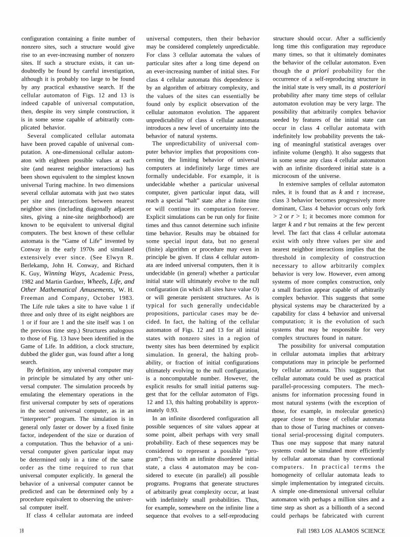
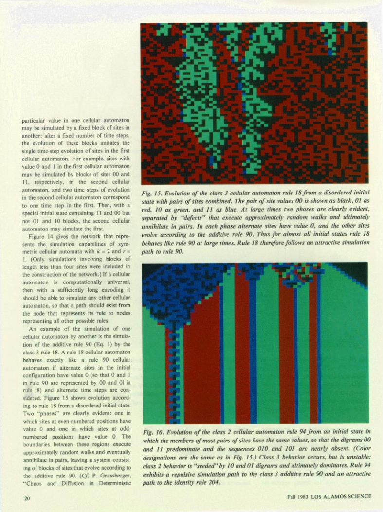
cellular Automata,” to be published inPhysica D.) Thus the simulation of rule 90by rule 18 may be considered an “attractive”one: starting from almost all initial states,rule 18 evolves toward states in which itsimulates rule 90. In general, one expectsthat some paths in the network of Fig. 14 areattractive, while the rest are repulsive. Theconsequences of a repulsive simulation pathare illustrated in Fig. 16: with special initialstates rule 94 behaves like rule 90, but anyimpurities in the initial states grow andeventually dominate the evolution of thesystem.

Class 1 cellular automata have an attract-ive simulation path to rule O (or its equiv-alents). Class 2 cellular automata have at-tractive simulation paths to the identity rule204. A conjecture for which some evidenceexists is that all class 3 rules exhibit attrac-tive simulations has to additive rules suchas 90 or 150. Simulation by blocking of sitevalues is analogous to a block spin orrenormalization group transformation: addi-tive rules have the special property that theyare invariant under such transformations. Asmentioned earlier, class 4 cellular automataare distinguished by the. presence of simula-tion paths leading to every other cellularautomaton rule. It is likely that no specificpath is distinguished as attractive.

Cellular automata of different classes maythus be distinguished by their limitingbehavior under simulation transformations.This approach suggests that classification ofthe qualitative behavior of cellular automatamay be related to determinations of equiv-alence of systems and problem classes incomputation theory. In general, one mayhope for fundamental connections betweencomputation theory and the theory of com-plex nonequilibrium statistical systems. In-formation theory forms a mathematical basisfor equilibrium statistical mechanics. Com-putation theory, which addresses time-de-pendent processes. may be expected to playa fundamental role in nonequilibrium statis-tical mechanics. ■

Los Alamos Science Fall 1983

Stephen Wolfram was born in London, England in 1959. He was educated at Eton College, OxfordUniversity, and the California Institute of Technology where he received his Ph.D. in theoretical physicsin 1979. He was a member of the faculty at Caltech from 1980 until he resigned in 1982. At that time hejoined the Institute for Advanced Study in Princeton, New Jersey. He has worked in various areas oftheoretical physics, including high-energy physics, cosmology, and statistical mechanics and has alsoworked in computer science, particularly in the area of symbolic computation. He received a MacArthurFellowship in 1981 and since 1982 has been a Visiting Staff Member of the Theoretical Division at LosAlamos.

Acknowledgments

I am grateful to many people for discussions and suggestions. I thank in particular my collaborators invarious cellular automaton investigations: O. Martin. J. Milnor, and A. Odlyzko. The research describedhere was supported in part by the Office of Naval Research under contract number N00014-80-C-0657.

Further Reading

John von Neumann. Edited and completed by Arthur W. Burks. Theory of Self-Reproducirg Automata.

Urbana: University of Illinois Press, 1966.

Arthur W. Burks, editor. Essays on Cellular Automata. Urbana: University of IIIinois Press, 1970.

Stephen Wolfram. ‘cStatistical Mechanics of Cellular Automata.” Reviews of Modern Physics55(1983):601

Stephen Wolfram. “Universality and Complexity in Cellular Automata.” The Institute for AdvancedStudy preprint (May 1983) and to be published in Physica D.

Stephen Wolfram, J. Doyne Farmer, and Tommaso Toffoli, editors. “Cellular Automata: Proceedings of

an Interdisciplinary Workshop (LOS Alamos; March 7-11. 1983).” TO be published in Physica D and tobe available separately from North-Holland Publishing Company.

21

.—..

HISTORICAL PERSPECTIVE

From Turing and von Neumannto the Present

by Necia G. Cooper

automaton—a mechanism that is rel-atively self-operating; a device or machinedes igned to fo l low automat ica l ly apredetermined sequence of operations orrespond to encoded instructions.

The notion of automata in the sense ofmachines that operate on their own fromencoded instructions is very ancient, and onemight say that mechanical clocks and musicboxes fall under this category. The idea ofcomputing machines is also very old. Forinstance. Pascal and Leibnitz outlined vari-ous schematics for such machines. In thelatter part of the 18th century Baron deKempelen built what was alleged to be thefirst chess-playing machine. Remarkable asit appeared. alas, it was a fake operated by aperson hidden within it!

The modern theory of automata can betraced to two giants in the field ofmathematics. Alan Turing and John vonNeumann. These two men laid much of thelogical foundation for the development ofpresent-day electronic computers, and bothwere involved in the practical design of realcomputing machines.

Before World War II Turing had provedthe logical limits of computability and on thebasis of this work had designed in idealizedterms a universal computer, a machine thatcould perform all possible numerical com-putations. This idealized machine is nowknown as a Turing machine. (All moderncomputers have capabilities equivalent tosome of the universal Turing machines.)During World War H Turing successfullyapplied his logical talent to the real andurgent problem of breaking the Nazi in-telligence code. a feat that played a crucialrole in the Allied victory.

Prior to World War II von Neumann wasaware of Turing’s work on computing ma-chines and realized how useful such ma-chines would be for investigating nonlinearproblems in mathematical physics, inparticular. the fascinating problem ofturbulence. Numerical calculations might,for example, elucidate the mysterious role oft h e R e y n o l d s n u m b e r i n t u r b u l e n tphenomena. (The Reynolds number givesroughly the ratio of the inertial forces to theviscous forces. A flow that is regular be-comes turbulent when this number is about2000.) He was convinced that the best

mathematics proceeds from empirical sci-ence and that numerical calculation on elec-tronic computers might provide a new kindof empirical data on the properties ofnonlinear equations. Stan Ulam suggests thatthe final impetus for von Neumann to workenergetically on computer methods and de-sign came from wartime Los Alamos, whereit became obvious that analytical work alonewas often not sufficient to provide evenqualitative answers about the behavior of anatomic bomb. The best way to construct acomputing machine thus presented a prac-tical as well as a theoretical problem.

Starting in 1944 von Neumann formulatedmethods of translating a set of mathematicalprocedures into a language of instructionsfor a computing machine. Before von Neu-mann’s work on the logical design of com-puters, the few existing electronic machineshad to be rewired for each new problem. VonNeumann developed the idea of a fixed “flowdiagram” and a stored “code,” or program,that would enable a machine with a fixed setof connections to solve a great variety ofproblems.

Von Neumann was also interested, as wasTuring, in discovering the logical elements

22 Fall 1983 LOS ALAMOS SCIENCE

Cellular Automata

HISTORICAL PERSPECTIVE—.

and organization required to perform someof the more general types of functions thathuman beings and other life forms carry outand in trying to construct, at least at an

abstract level, machines that contained suchcapabilities. But whereas Turing was prima-rily interested in developing “intelligent” au-tomata that would imitate the thinking anddecision-making abilities of the human brain,von Neumann focused on the broader prob-lem of developing a general theory of com-plicated automata, a theory that would en-compass both natural automata (such as thehuman nervous system and living organisms)and artificial automata (such as digital com-puters and communication networks).

What is meant by the term “com-plicated”? As von Neumann put it, it is not aquestion of how complicated an object is butrather of how involved or difficult itspurposive operations are. In a series oflectures delivered at the University of Illinoisin 1949, von Neumann explored ideas aboutwhat constitutes complexity and what kindof a theory might be needed to describecomplicated automata. He suggested that anew theory of information would be neededfor such systems, one that would bear aresemblance to both formal logic andthermodynamics. It was at these lecturesthat he explained the logical machinerynecessary to construct an artificial automa-ton that could carry out one very specificcomplicated function, namely, self-reproduc-tion. Such an automaton was also logicallycapable of constructing automata more com-plex than itself. Von Neumann actuallybegan constructing several models of self-reproducing automata. Based on an inspiredsuggestion by Ulam, one of these models wasin the form of a “cellular” automaton (seethe preceding article in this issue by StephenWolfram for the definition of a cellularautomaton).

From the Illinois lectures it is clear thatvon Neumann was struggling to arrive at acorrect definition of complexity. Althoughhis thoughts were still admittedly vague, they


do seem, at least in some respects, related tothe present efforts of Wolfram to find univer-sal features of cellular automaton behaviorand from these to develop new laws,analogous to those of thermodynamics, todescribe self-organizing systems.

Von Neumann suggested that a theory ofinformation appropriate to automata wouldbuild on and go beyond the results of Turing,Godel, Szilard, and Shannon.

Turing had shown the limits of what canbe done with certain types of informa-tion—namely, anything that can be de-scribed in rigorously logical terms can bedone by an automaton. and, conversely.

anything that can be done by an automatoncan be described in logical terms. Turingconstructed. on paper, a universal automa-ton that could perform anything that anyother automaton could do. It consisted of afinite automaton, one that exists in a finitenumber of states, plus an indefinitely ex-tendible tape containing instructions. “Theimportance of Turing’s research is just this:”said von Neumann, “that if you construct anautomaton right, then any additional require-ments about the automaton can be handledby sufficiently elaborate instructions. This istrue only if [the automaton] is sufficientlycomplicated. if it reaches a certain minimumlevel of complexity” (John von Neumann,Theory of Self-Reproducing Automata,

edited and completed by Arthur W. Burks,University of Illinois Press, 1966, p. 50).

Turing also proved that there are somethings an automaton cannot do. For exam-ple, “YOU cannot construct an automatonwhich can predict in how many steps an-other automaton which can solve a certainproblem will actually solve it. . . . In otherwords, you can build an organ which can doanything that can be done. but you cannotbuild an organ which tells you whether it canbe done” (ibid., p. 51). This result of Turing’sis connected with Godel’s work on the

hierarchy of types in formal logic. VonNeumann related this result to his notion ofcomplexity. He suggested that for objects of

low complexity, it is easier to predict theirproperties than to build them, but for objectsof high complexity, the opposite is true.

Von Neumann stated that the new theory

of information should include not only thestrict and rigorous considerations of formallogic but also statistical considerations. Thereason one needs statistical considerations isto include the possibility of failure. Theactual structure of both manmade andartificial automata is dictated by the need toachieve a state in which a majority of allfailures will not be lethal. To include failure,one must develop a probabilistic system oflogic. Von Neumann felt that the theory ofentropy and information in thermodynamicsand Shannon’s information theory would berelevant.

Szilard had shown in 1929 that entropy ina physical system measures the lack ofinformation; it gives the total amount ofmissing information on the microscopicstructure of the system. Entropy defined as aphysical quantity measures the degree ofdegradation suffered by any form of energy.“There are strong indications that informa-tion is similar to entropy and that thedegenerative processes of entropy areparalleled by degenerative processes in theprocessing of information” (ibid., p. 62).

Shannon’s work focused on the problemof transmitting information. He had de-veloped a quantitative theory of measuringthe capacity of a communication channel, atheory that included the role of redundancy.Redundancy makes it possible to correcterrors and “is the only thing which makes itpossible to write a text which is longer than,say, ten pages. In other words, a languagewhich has maximum compression wouldactually be completely unsuited to conveyinginformation beyond a certain degree of com-plexity, because you could never find outwhether a text is right or wrong” (ibid., p.60).

Von Neumann emphasized the ability ofliving organisms to operate across errors.Such a system “is sufficiently flexible and

23


well organized that as soon as an errorshows up in any one part of it, the systemautomatically senses whether this error mat-ters or not. If it doesn’t matter, the systemcontinues to operate without paying anyattention to it. If the error seems to beimportant, the system blocks that region out.by-passes it and proceeds along other chan-nels. The system then analyzes the regionseparately at leisure and corrects what goeson there. and if correction is impossible thesystem just blocks the region off and by-passes it forever. . . .

“To apply the philosophy underlyingnatural automata to artificial automata wemust understand complicated mechanismsbetter than we do, we must have elaboratestatistics about what goes wrong, and wemust have much more perfect statisticalinformation about the milieu in which amechanism lives than we now have. Anautomaton cannot be separated from themilieu to which it responds” (ibid., pp .71-72).

From artificial automata “one gets a verystrong impression that complication, orproductive potentiality in an organization, isdegenerative, that an organization whichsynthesizes something is necessarily morecomplicated. of a higher order, than theorganization it synthesizes” (ibid., p. 79).

But life defeats degeneracy. Although thecomplicated aggregation of many elementaryparts necessary to form a living organism isthermodynamically highly improbable, oncesuch a peculiar accident occurs. the rules ofprobability do not apply because the or-ganism can reproduce itself provided themilieu is reasonable—and a reasonablemilieu is thermodynamically much less im-probable. Thus probability leaves a loopholethat is pierced by self-reproduction.

Is it possible for an artificial automaton toreproduce itself? Further, is it possible for amachine to produce something that is morecomplicated than itself in the sense that theoffspring can perform more difficult andinvolved tasks than the progenitor? These

24

A three-dimensional object grown from a single cube to the thirtieth generation (darkcubes). The model shows only one octant of the three-dimensional structure. This

figure and the two others illustrating this article are from R. G. Schrandt and S. M.Ulam, “On Recursively Defined Geometrical Objects and Patterns of Growth,” LosAlamos Scientific Laboratory report LA-3762, November 1967 and are also reprintedin Arthur W. Burks, editor, Essays on Cellular Automata, University of Illinois Press,1970.

questions arise from looking at natural au-tomata. In what sense can a gene contain adescription of the human being that willcome from it? How can an organism at alow level in the phylogenetic order developinto a higher level organism?

From his comparison of natural andartificial automata, von Neumann suggestedthat complexity has one decisive property,namely, a critical size below which theprocess of synthesis is degenerative andabove which the process is explosive in thesense that an automaton can produce others

that are more complex and of higher poten-tiality than itself. However, to get beyond therealm of vague statements and develop acorrect formulation of complexity, he felt itwas necessary to construct examples thatexhibit the “critical and paradoxicalproperties of complication” (ibid., p. 80).

To this end he set out to construct, inprinciple, self-reproducing automata, autom-ata “which can have outputs somethinglike themselves” (ibid., p. 75). (All artificial

automata discussed up to that point. such asTuring machines, computing machines, and


Cellular Automata


(a) (b)

the network of abstract neurons discussed byMcCulloch and Pitts (“A Logical Calculusof the Ideas Immanent in Nervous Activity,”Bulletin of Mathematical Biophysics, 1943),had inputs and outputs of completely dif-ferent media than the automata them-selves.)

"There is no question of producing matterout of nothing. Rather, one imagines au-tomata which can modify objects similar tothemselves, or effect syntheses by picking upparts and putting them together, or takesynthesized entities apart” (ibid., p. 75).

Von Neumann drew up a list of unam-

biguously defined parts for the kinematicmodel of a self-reproducing automaton. Al-though this model ignored mechanical andchemical questions of force and energy, it didinvolve problems of movement, contact,positioning, fusing, and cutting of elements.

Von Neumann changed his initial ap-proach after extensive discussions withUlam. Ulam suggested that the proof ofexistence and construction of a self-

reproducing automaton might be done in asimpler, neater way that retained the logicaland combinatorial aspects of the problembut eliminated complicated aspects ofgeometry and motion. Ulam’s idea was toconstruct the automaton in an indefinitelylarge space composed of cells. In twodimensions such a cellular structure is equiv-alent to an infinite checkerboard. The ele-ments of the automaton are a set of allow-able states for each cell. including an empty,

A “contest’’ between two patterns, one of lines within squares (shaded) and one of dotswithin squares, growing in a 23 by 23 checkerboard. Both patterns grow by a recursiverule stating that the newest generation (represented by diagonal lines or by dots in anx shape) may occupy a square if that square is orthogonally contiguous to one andonly one square occupied by the immediately preceding generation (represented byperpendicularly bisecting lines or by dots in a + shape). In addition, no piece of eitherpattern may survive more than two generations. Initially, the line pattern occupiedonly the lower left corner square, and the dot pattern occupied only the squareimmediately to the left of the upper right corner square. (a) At generation 16 the twopatterns are still separate. (b) At generation 25 the two patterns engage. (c)At 32generations the dot pattern has penetrated enemy territory. (d) At 33 generations thedot pattern has won the contest.

or quiescent, state, and a transition rule fortransforming one state into another. The ruledefines the state of a cell at time interval t+1in terms of its own state and the states ofcertain neighboring cells at time interval t.Motion is replaced by transmitting informa-tion from cell to cell; that is, the transitionrule can change a quiescent cell into anactive cell.

Von Neumann’s universal self-reproduc-ing cellular automaton, begun in 1952, was arather baroque construction in which eachcell had twenty-nine allowable states and a

LOS ALAMOS SCIENCE Fall 1983 25


neighborhood consisting of the four cellsorthogonal to it. Influenced by the work ofMcCulloch and Pitts, von Neumann used aphysiological simile of idealized neurons tohelp define these states. The states andtransition rules among them were designedto perform both logical and growth opera-tions. He recognized. of course. that hisconstruction might not be the minimal oroptimal one, and it was later shown byEdwin Roger Banks that a universal self-reproducing automaton was possible withonly four allowed states per cell.

The logical trick employed to make theautomaton universal was to make it capableof reading any axiomatic description of anyother automaton, including itself, and toinclude its own axiomatic description in itsmemory. This trick was close to that used byTuring in his universal computing machine.The basic organs of the automaton includeda tape unit that could store information onand read from an indefinitely extendiblelinear array of cells, or tape, and a construct-ing unit containing a finite control unit andan indefinitely long constructing arm thatcould construct any automaton whose de-scription was stored in the tape unit. Realiza-tion of the 29-state self-reproducing cellularautomaton required some 200,000 cells.

Von Neumann died in 1957 and did notcomplete this construction (it was completedby Arthur Burks). Neither did he completehis plans for two other models of self-reproducing automata. In one, based on the29-state cellular automaton, the basic ele-ment was to be neuron-like and have fatiguemechanisms as well as a threshold for excita-tion. The other was to be a continuous modelof self-reproduction described by a system ofnonlinear partial differential equations of thetype that govern diffusion in a fluid. VonNeumann thus hoped to proceed from thediscrete to the continuous. He was inspiredby the abilities of natural automata andemphasized that the nervous system was notpurely digital but was a mixed analog-digitalsystem.

26

Much effort since von Neumann’s timehas gone into investigating the simulationcapabilities of cellular automata. Can onedefine appropriate sets of states and transi-tion rules to simulate natural phenomena’?Ulam was among the first to use cellularautomata in this way. He investigatedgrowth patterns of simple finite systems,simple in that each cell had only two statesand obeyed some simple transition rule.Even very simple growth rules may yieldhighly complex patterns, both periodic andaperiodic. “The main feature of cellularautomata,” Ulam points out, “is that simplerecipes repeated many times may lead tovery complicated behavior. Information

analysts might look at some final pattern andinfer that it contains a large amount ofinformation, when in fact the pattern isgenerated by a very simple process. Perhapsthe behavior of an animal or even ourselvescould be reduced to two or three pages ofsimple rules applied in turn many times!"(private conversation. October 1983).Ulam’s study of the growth patterns ofcellular automata had as one of its aims “tothrow a sidelight on the question of howmuch ‘information’ is necessary to describethe seemingly enormously elaborate struc-tures of living objects” (ibid.). His work withHolladay and with Schrandt on an electroniccomputing machine at Los Alamos in 1967produced a great number of such patterns.Properties of their morphology were

surveyed in both space and time. Ulam andSchrandt experimented with “contests” inwhich two starting configurations were al-lowed to grow until they collided. Then afight would ensue, and sometimes one con-figuration would annihilate the other. Theyalso explored three-dimensional automata.

Another early investigator of cellularautomata was Ed Fredkin. Around 1960 hebegan to explore the possibility that allphysical phenomena down to the quantummechanical level could be simulated bycellular automata. Perhaps the physicalworld is a discrete space-time lattice of

A pattern grown according to a recursiverule from three noncontiguous squaresat the vertices of an approximately equi-lateral triangle. A square of the nextgeneration is formed if (a) it is con-tiguous to one and only one square of thecurrent generation, and (b) it touches noother previously occupied square exceptif the square should be its “grand-parent. ” In addition, of this set of pro-spective squares of the (n+l)th genera-tion satisfying condition (b), all squaresthat would touch each other areeliminated. However, squares that havethe same parent are allowed to touch.

information bits that evolve according tosimple rules. In other words, perhaps theuniverse is one enormous cellular automa-ton.

There have been many other workers inthis field. Several important mathematicalresults on cellular automata were obtainedby Moore and Holland (University of Mich-igan) in the 1960s. The “Game of Life,” anexample of a two-dimensional cellularautomaton with very complex behavior, wasinvented by Conway (Cambridge University)around 1970 and extensively investigated forseveral years thereafter.


Cellular Automata

Cellular automata have been used in bio-logical studies (sometimes under the namesof “tessellation automata” or “homogeneousstructures”) to model several aspects of thegrowth and behavior of organisms. Theyhave been analyzed as parallel-processingcomputers (often under the name of “iter-ative arrays”). They have also been appliedto problems in number theory under thename “stunted trees” and have been con-sidered in ergodic theory, as endomorphismsof the “dynamical” shift system.

A workshop on cellular automata at LosAlamos in March 1983 was attended byresearchers from many different fields. Theproceedings of this workshop will be pub-lished in the journal Physica D and will alsobe issued as a book by North-HollandPublishing Co.

In all this effort the work of StephenWolfram most closely approaches von Neu-mann’s dream of abstracting from examplesof complicated automata new concepts rele-

vant to information theory and analogous tothe concepts of thermodynamics. Wolframhas made a systematic study of one-dimen-

sional cellular automata and has identifiedfour general classes of behavior, as describedin the preceding article.

Three of these classes exhibit behavioranalogous to the limit points, limit cycles,and strange attractors found in studies ofnonlinear ordinary differential equations andtransformation iterations. Such equations

characterize dissipative systems. systems inwhich structure may arise spontaneouslyeven from a disordered initial state. Fluidsand living organisms are examples of suchsystems. (Non-dissipative systems, in con-trast, tend toward disordered states of max-imal entropy and are described by the lawsof thermodynamics.) The fourth class mim-ics the behavior of universal Turing ma-chines. Wolfram speculates that his identifi-cation of universal classes of behavior incellular automata may represent a first step

Further Reading

John von Neumann. Theory of Self-Reproducing Automata. Edited and completed by Arthur W. Burks.Urbana: University of Illinois Press. 1966. Part I is an edited version of the lectures delivered at theUniversity of Illinois. Part II is von Neumann’s manuscript describing the construction of his 29-stateself-reproducing automaton.

Arthur W. Burks, editor. Essays on Cellular Automata. Urbana: University of Illinois Press. 1970. Thisvolume contains early papers on cellular automata including those of Ulam and his coworkers.

Andrew Hodges, “Alan Turing: Mathematician and Computer Builder.” New Scientist. 15 September1983, pp. 789-792. This contains a wonderful illustration, “A Turing Machine in Action.”

Martin Gardner. "On Cellular Automata, Self-Reproduction, the Garden of Eden. and the Game ‘Life,’ “Scientific American, October 1971.

The following publications deal with complexity per se:

W. A. Beyer, M. L. Stein, and S. M. Ulam. “The Notion of Complexity.” Los Alamos ScientificLaboratory report LA-4822. December 1971.


in the formulation of general laws for com-plex self-organizing systems. He says thatwhat he is looking for is a new con-cept—maybe it will be complexity or maybesomething else—that like entropy will bealways increasing (or decreasing) in such asystem and will be manifest in both themicroscopic laws governing evolution of thesystem and in its macroscopic behavior. Itmay be closest to what von Neumann had inmind as he sought a correct definition of’complexity. We can never know. We can

Acknowledgment

I wish to thank Arthur W. Burks for per-mission to reprint quotations from Theory ofSelf-Reproducing Automata. We areindebted to him for editing and completingvon Neumann’s manuscripts in a mannerthat retains the patterns of thought of a greatmind.

S. Winograd. Arithmetic Complexity of Computations. Philadelphia: Society of Industrial and AppliedMathematics. 1980.

LOS ALAMOS SCIENCE Fall 1983 27

cellular automata - federation of american scientists

Documents