centralized approach for multi-node localization and
TRANSCRIPT

Abstract: A new algorithm for the localization and identification of multi-node systems has been introduced in this
paper; this algorithm is based on the idea of using a beacon provided with a distance sensor and IR sensor to calculate the
location and to know the identity of each visible node during scanning. Furthermore, the beacon is fixed at middle of the
frame bottom edge for a better vision of nodes. Any detected node will start to communicate with the neighboring nodes
by using the IR sensors distributed on its perimeter; that information will be used later for the localization of
invisible nodes. The performance of this algorithm is shown by the implementation of several simulations.
Index Terms— Beacon node, Identification, Localization, Multi-node.
I. INTRODUCTION
Wireless sensor networks have attracted a lot of
attention due to their important role and increased
utilization in many military and civilian domains
[1-3]. Localization is one of the most important
challenges in the development of wireless sensor
networks [4-5], the reason for that is, collecting
data without locations will make these data
geographically meaningless [6-7].
Wireless sensor network consist of many sensor
nodes that each contains sensors, battery,
processor and other devices that may be needed
[8]. Every node in wireless sensor network
collects data and either forwards them to a central
node to calculate their locations and this will be
called a centralized architecture [9-10] or use
these data to localize itself and then forward the
data and this will be called a distributed
architecture [11-12].
Localization can be relative, absolute or a
combination of them [13-14] .Relative
localization is usually based on the dead
reckoning (that is, monitoring the wheel
revolutions to find the distance from a known
starting location). The unbounded accumulation
of errors is the main disadvantage of this method
and in the case of movement, relative localization
is preferable. On the other hand, absolute
localization depends on the satellite signals,
beacons, landmarks or map matching to find the
location of a node. GPS is one of the used
methods as an example of the absolute
localization but it can be used only outdoor and it
is inaccurate for mobile nodes [15-16].
In this paper, we introduce a combination of both
absolute and relative localization; the absolute
localization is represented by the beacon which
scans the environment looking for visible nodes.
On the other hand, the relative localization is
generated by visible nodes while exploring the
environment in search of their neighbors. Also, in
this paper we use the centralized architecture
where all the information results from scanning
the environment by both of the beacon and visible
nodes is collected in the beacon to construct two
tables which will be used later to localize the
invisible nodes. The details of this algorithm will
be discussed in section II and the related work in
section III; section IV shows the simulation
results of this algorithm. Finally the conclusion
will be in section V.
II. RELATED WORK
When we talk about obtaining location
information, the first thing came into our mind is
the global positioning system (GPS) proposed by
B. Hofmann-Wellenhof [17]. But due to its high
cost and in ability to work in indoor environment,
a lot of algorithms concerns with localization
Centralized approach for multi-node localization and
identification
Electrical Engineering Department
University of Basrah
Basrah, Iraq
Ramzy S. Ali
Electrical Engineering Department
University of Basrah
Basrah, Iraq
Abdulmuttalib T. Rashid Electrical Engineering Department
University of Basrah
Basrah, Iraq
178
Iraqi Journal for Electrical and Electronic EngineeringOriginal Article
Open Access
Received: 2 September 2016 Revised: 25 October 2016 Accepted: 30 October 2016
DOI: 10.37917/ijeee.12.2.8 Vol. 12| Issue 2 | December 2016
Ola A. Hasan

according to the type of information used to
localize nodes have been studied [9]. Many of
those algorithms lay on the range-based schemes
which use the ranged measurements strategies
such as the received signal strength (RSS), angle
of arrival (AOA), time of arrival (TOA) and time
difference of arrival (TDOA) to compute either
the distance or angle between two nodes [18]. As
an example is the algorithm proposed by P. Bahl
et al. [19] which is a method to convert the RSS
to a distance and then uses the triangulation to
calculate the node's position. Some other papers
lay on the range free strategies such as:
approximate point in triangle (APIT), DV-Hop
and centroid. Those strategies take into account
the connectivity among nodes to achieve
localization [9]. For example, centroid algorithm
proposed by N. Bulusu et al. [20] which uses a
centroid formula to localize the nodes after
receiving the locations of beacons. The range
based algorithms are more accurate than the range
free but the range free algorithms are less in the
term of complicity and cost. Therefore, some
researchers focused on proposing methods that
combine the benefits of the range based and range
free both and considered to be more accurate than
the range free and less cost and complicity than
the range based. An example for that is the
algorithm proposed by A. T. Rashid et al. [21]
where a beacon is provided with distance sensor
to determine the locations of visible nodes and
construct clusters; those clusters will be
compared later with unit disk graph for each node
which constructed by the connectivity among
nodes to know the identity of them. In this paper
we will propose an algorithm that is better than
the algorithm proposed by A. T. Rashid et al. in
the case of visibility, accuracy and computation
complicity.
III. LOCATION AND IDENTITY COMBINATION
ALGORITHM
In this algorithm, the beacon which is located at
middle of the frame bottom edge contains a
distance sensor and IR sensor pair (transmitter
and receiver) as shown in Fig. 1; those sensors
are fixed on a servo motor which rotates at 180⁰ .
Also, there are n of IR sensors distributed evenly
on the perimeter of every node in the system. The
location and identity of each node are found
according to the following subsections:
Fig.1, The construction of the Beacon node.
A. Localization of Visible Nodes: The beacon
scans the environment at 180⁰ searching for any
node as shown in Fig.2, if the beacon detects a
node, the coordinates of this node will be
calculated as in the equation below:
xi = xb + dbi * cos αb
i
(1)
yi = yb + dbi * sin αb
i
Where dbi and αb
i are the distance and the
detecting angle of node i respectively, (xb, yb) are
the coordinates of the beacon and (xi, yi) are the
coordinates of node i.
B. Identity of Visible Nodes: After detecting a
node, the beacon uses the IR sensor pair to send
an infrared signal to identify itself and waits for
the node to reply with its identity number. Each
node is provided with n of IR sensor pairs which
numbered in sequentially form starting from the
reference IR sensor as shown in Fig.3; the angle
K between each two neighboring sensor pairs are
equal and they are computed as in equation2: K = 360 / n (2)
179
Ola A. Hasan Vol. 12| Issue 2 | December 2016
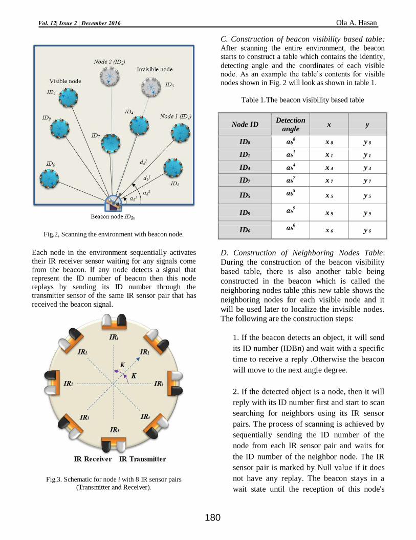
Fig.2, Scanning the environment with beacon node.
Each node in the environment sequentially activates their IR receiver sensor waiting for any signals come from the beacon. If any node detects a signal that represent the ID number of beacon then this node replays by sending its ID number through the transmitter sensor of the same IR sensor pair that has
received the beacon signal.
Fig.3. Schematic for node i with 8 IR sensor pairs
(Transmitter and Receiver).
C. Construction of beacon visibility based table: After scanning the entire environment, the beacon starts to construct a table which contains the identity,
detecting angle and the coordinates of each visible node. As an example the table’s contents for visible nodes shown in Fig. 2 will look as shown in table 1.
Table 1.The beacon visibility based table
Node ID Detection
angle x y
ID8 αb8
x 8 y 8
ID1 αb1 x 1 y 1
ID4 αb4 x 4 y 4
ID7 αb7 x 7 y 7
ID5 αb
5 x 5 y 5
ID9 αb
9 x 9 y 9
ID6 αb
6 x 6 y 6
D. Construction of Neighboring Nodes Table:
During the construction of the beacon visibility
based table, there is also another table being
constructed in the beacon which is called the
neighboring nodes table ;this new table shows the
neighboring nodes for each visible node and it
will be used later to localize the invisible nodes.
The following are the construction steps:
1. If the beacon detects an object, it will send
its ID number (IDBn) and wait with a specific
time to receive a reply .Otherwise the beacon
will move to the next angle degree.
2. If the detected object is a node, then it will
reply with its ID number first and start to scan
searching for neighbors using its IR sensor
pairs. The process of scanning is achieved by
sequentially sending the ID number of the
node from each IR sensor pair and waits for
the ID number of the neighbor node. The IR
sensor pair is marked by Null value if it does
not have any replay. The beacon stays in a
wait state until the reception of this node's
180
Ola A. Hasan Vol. 12| Issue 2 | December 2016
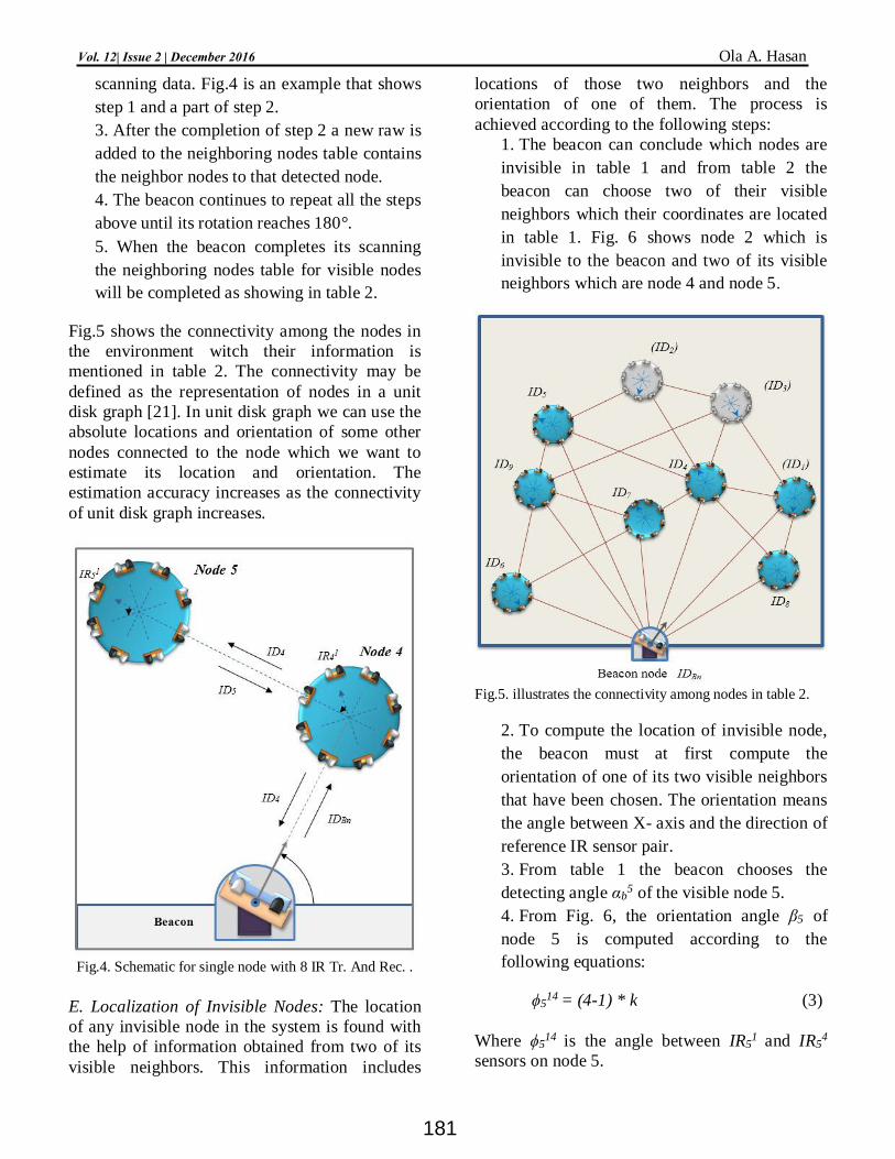
scanning data. Fig.4 is an example that shows
step 1 and a part of step 2.
3. After the completion of step 2 a new raw is
added to the neighboring nodes table contains
the neighbor nodes to that detected node.
4. The beacon continues to repeat all the steps
above until its rotation reaches 180°.
5. When the beacon completes its scanning
the neighboring nodes table for visible nodes
will be completed as showing in table 2.
Fig.5 shows the connectivity among the nodes in
the environment witch their information is
mentioned in table 2. The connectivity may be
defined as the representation of nodes in a unit
disk graph [21]. In unit disk graph we can use the
absolute locations and orientation of some other
nodes connected to the node which we want to
estimate its location and orientation. The
estimation accuracy increases as the connectivity
of unit disk graph increases.
Fig.4. Schematic for single node with 8 IR Tr. And Rec. .
E. Localization of Invisible Nodes: The location
of any invisible node in the system is found with
the help of information obtained from two of its
visible neighbors. This information includes
locations of those two neighbors and the
orientation of one of them. The process is
achieved according to the following steps: 1. The beacon can conclude which nodes are
invisible in table 1 and from table 2 the
beacon can choose two of their visible
neighbors which their coordinates are located
in table 1. Fig. 6 shows node 2 which is
invisible to the beacon and two of its visible
neighbors which are node 4 and node 5.
Fig.5. illustrates the connectivity among nodes in table 2.
2. To compute the location of invisible node,
the beacon must at first compute the
orientation of one of its two visible neighbors
that have been chosen. The orientation means
the angle between X- axis and the direction of
reference IR sensor pair.
3. From table 1 the beacon chooses the
detecting angle αb5 of the visible node 5.
4. From Fig. 6, the orientation angle β5 of
node 5 is computed according to the
following equations:
ϕ514 = (4-1) * k (3)
Where ϕ514 is the angle between IR5
1 and IR54
sensors on node 5.
181
Ola A. Hasan Vol. 12| Issue 2 | December 2016

σ = 180 - ϕ514 (4)
β5 = σ + αb5 (5)
5. The localization of invisible node 2 as in
Fig.7 is achieved according to set of equations
as follow:
L = ((y5 – y4)2 + (x5 – x4)2)1/2 (6)
Where L is the distance between node 4 and node
5.
ϕ556 = (6 – 5) * K (7)
Where ϕ556 is the angle between IR5
5 (the sensor
which received the signal from node 4) and IR56
(the sensor which received the signal from node
2) on node 5.
ϕ412 = (2 – 1) * K (8)
Where ϕ412 is the angle between IR4
1 (the sensor
which received the signal from node 2) and IR42
(the sensor which received the signal from node
5) on node 4.
ϕ282 = 180 - (ϕ5
56 + ϕ412) (9)
ϕ282 represents the angle between the IR sensors
which received the signals from nodes 5 and 4.
By using the sin low:
L / sin ϕ282 = R / sin ϕ4
12 (10)
Where R is the distance between node 5 and node
2.
ϕ561 = (9 – 6) * K (11)
ϕ561 is the angle between the orientation of node 5
and the distance between node 2 and node 5. The
number 9 represents (8+1), where 8 is total
number of IR sensor pairs on each node.
θ = β5 – ϕ561 (12)
The coordinates (x2, y2) of the invisible node 2
will be as below:
x2 = x5 + R * cos θ
(13)
y2 = y5 + R * sin θ
Fig.6, the orientation of node 5.
Fig.7. Localization of node 2.
182
Ola A. Hasan Vol. 12| Issue 2 | December 2016

Table 2. The neighboring nodes table
IV. THE SIMULATION RESULTS
Numerical simulations have been implemented by
using visual basic 2012 programming language. It
is repeated over 100 times on different sizes of
networks ranging from 5 to 50 nodes and also
repeated for three nodes' radiuses which are 10,
15 and 20 pixels. Nodes are distributed on an area
of 500*500 pixels and each node has a unique ID
number. The results of our algorithm are
compared with the robotic cluster matching
algorithm [21]; the robotic cluster matching
algorithm uses a combination of absolute and
relative sources for localization and orientation of
multi-robot systems. The absolute information is
obtained from the beacon which is a distance
sensor located at the left bottom corner of the
frame and rotates at 90⁰. The beacon scans the
environment for visible robots that will be used to
form clusters. On the other hand, the relative
information is obtained from robots where every
robot scans the environment looking for its
neighbors to construct a unit disk graph. Finally,
by the matching of clusters and the unit disk
graph of each robot the visible robots will be
localized. In our algorithm the beacon is provided
with a distance and IR sensors; it is located at
middle of the frame bottom edge and rotates at
180⁰. Fig.8, Fig. 9, and Fig. 10 study the effects
of 10, 15 and 20 pixels node radius respectively
on the visibility (the number of visible nodes) of
30 nodes environment, where the black nodes are
visible to the beacon while the gray ones are not.
It is obvious that the visibility decreases as the
radius of nodes increases. The increasing in
visibility means that the number of nodes which
localized by the beacon increased and thus leads
to an increase in number of nodes which have
accurate locations.
Fig. 8, Illustration the effects of nodes with 10 pixels radius on 30 nodes environment
Fig.11 shows a comparison between the visibility
percentage of our algorithm and the robotic
IR1 IR
2 IR3 IR
4 IR
5 IR
6 IR
7 IR
8
ID8 Null Null Null ID1 ID4 Null IDBn Null
ID1 ID8 Null Null Null Null ID3 ID4 IDBn
ID4 ID2 ID5 ID7 IDBn ID8 ID1 Null ID3
ID7 Null ID9 ID6 IDBn Null Null ID4 Null
ID5 Null Null ID9 IDBn ID4 ID2 Null Null
ID9 ID6 IDBn ID7 ID3 ID5 Null Null Null
ID6 Null IDBn ID7 ID9 Null Null Null Null
183
Ola A. Hasan Vol. 12| Issue 2 | December 2016
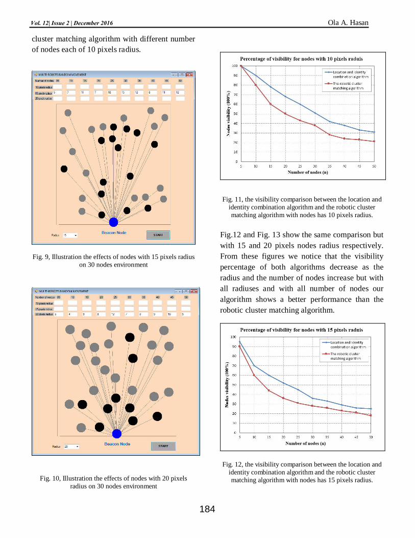
cluster matching algorithm with different number
of nodes each of 10 pixels radius.
Fig. 9, Illustration the effects of nodes with 15 pixels radius
on 30 nodes environment
Fig. 10, Illustration the effects of nodes with 20 pixels
radius on 30 nodes environment
Fig. 11, the visibility comparison between the location and
identity combination algorithm and the robotic cluster
matching algorithm with nodes has 10 pixels radius.
Fig.12 and Fig. 13 show the same comparison but
with 15 and 20 pixels nodes radius respectively.
From these figures we notice that the visibility
percentage of both algorithms decrease as the
radius and the number of nodes increase but with
all radiuses and with all number of nodes our
algorithm shows a better performance than the
robotic cluster matching algorithm.
Fig. 12, the visibility comparison between the location and
identity combination algorithm and the robotic cluster
matching algorithm with nodes has 15 pixels radius.
184
Ola A. Hasan Vol. 12| Issue 2 | December 2016
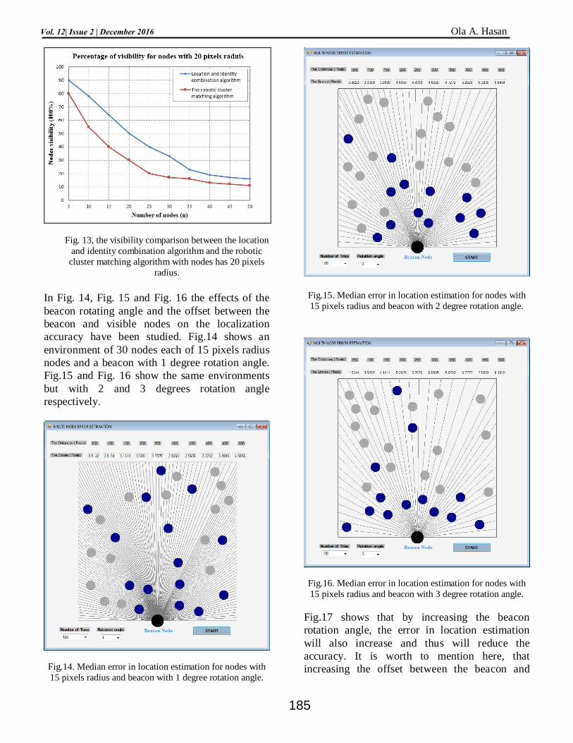
Fig. 13, the visibility comparison between the location
and identity combination algorithm and the robotic
cluster matching algorithm with nodes has 20 pixels
radius.
In Fig. 14, Fig. 15 and Fig. 16 the effects of the
beacon rotating angle and the offset between the
beacon and visible nodes on the localization
accuracy have been studied. Fig.14 shows an
environment of 30 nodes each of 15 pixels radius
nodes and a beacon with 1 degree rotation angle.
Fig.15 and Fig. 16 show the same environments
but with 2 and 3 degrees rotation angle
respectively.
Fig.14. Median error in location estimation for nodes with
15 pixels radius and beacon with 1 degree rotation angle.
Fig.15. Median error in location estimation for nodes with
15 pixels radius and beacon with 2 degree rotation angle.
Fig.16. Median error in location estimation for nodes with
15 pixels radius and beacon with 3 degree rotation angle.
Fig.17 shows that by increasing the beacon
rotation angle, the error in location estimation
will also increase and thus will reduce the
accuracy. It is worth to mention here, that
increasing the offset between the beacon and
185
Ola A. Hasan Vol. 12| Issue 2 | December 2016

visible nodes will also cause an increasing in the
error average.
Fig. 17, the accuracy of localization for different rotating
angles.
V. CONCLUSIONS
In this paper, an algorithm for multi-node
localization system has been introduced; it uses
the idea of centralized architecture where all the
locations computation is done in a centralized
station which is the beacon. In this algorithm, the
beacon also serves as a source of absolute
information during the environment scanning in
search of visible nodes. The source of relative
information is represented by the nodes where
each node scans the environment to find its
neighbors.
The position of beacon in our algorithm at
middle of the frame bottom edge has highlighted
the important role of this position on the nodes
visibility average. So, as compared with the
robotic cluster matching algorithm, our algorithm
shows an increase in the visibility average
meaning that more accuracy in location
estimation will be obtained. Also, our proposed
algorithm shows a better performance than the
robotic cluster matching algorithm in addressing
the nodes under the effects of different
parameters such as the rotating angle of beacon,
nodes radius and the size of network.
The proposed algorithm in this paper deals with
nodes only. So, as an improvement we suggest to
add a separate section for the orientation
calculation to involve even the robots. Another
suggestion is to add a beacon at middle of the
frame upper edge to have more visibility average.
REFERENCES
[1] M. Li, and Y. Lu, "Angle of arrival estimation for
localization and communication in wireless networks," 16th
European signal processing conference (EUSIPCO 2008),
pp. 25-29, 2008.
[2] Y. Bokareva, W. Hu, S. Kanhere, B. Ristic, N. Gordon,
T. Bessell, M. Rutten and S. Jha, "Wireless Sensor
Networks for Battlefield Surveillance," Land Warfare
Conference 2006.
[3] Q. I. Ali, A. Abdulmaowjod and H. M. Mohammed,
"Simulation and performance study of wireless sensor
network (WSN) using MATLAB," Iraq J. Electrical and
electronical engineering, vol.7, no. 2, pp. 112-119, 2011.
[4] N. Dhopre, and Sh. Y. Gaikwad, "Localization of
wireless sensor networks with ranging quality in woods,"
International journal of innovative research in computer and communication engineering, vol. 3, no. 4, pp.2893-2896,
2015.
[5] P.K. Singh, B. Tripathi, and N. P. Singh, "Node
localization in wireless sensor network," International
Journal of Computer Science and Information
Technologies, vol. 2, no. 6, pp. 2568-2572, 2011.
[6] G. S. Klogo,and J. D. Gadze, "Energy Constraints of
Localization Techniques in Wireless Sensor Networks
(WSN): A Survey," International Journal of Computer
Applications, vol. 75, no. 9, pp. 0975 – 8887, March 2013.
[7] J. Zhang, H. Li and J. Li, "An Improved CPE
Localization Algorithm for Wireless Sensor Networks,"
International Journal of Future Generation Communication
and Networking, vol.8, no. 1, pp. 109-116, 2015.
[8] J. N. S.,and M. R. Mundada, "Localization techniques
for wireless sensor networks," International journal of
engineering and technical research (IJETR), vol.3, no. 1,
pp. 30-36, 2015. [9] Y. Shang, W. Ruml, Y. Zhang, and M. P. J. Fromherz,
"Localization from mere connectivity," ACM symposium
on mobile Ad Hoc networking and computing, pp. 201-212,
2003 .
[10] A. Pal, "Localization Algorithms in Wireless Sensor
Networks: Current Approaches and Future Challenges,"
Network Protocols and Algorithms, vol. 2, no. 1, pp.45-73,
2010.
[11] K. Langendoen, and N. Reijers, "Distributed
localization in wireless sensor networks: A quantitative
comparison," Computer networks, vol.43, no. 4, pp. 499-
518, 2003.
[12] P.D.Patil, and R.S.Patil, " Distributed Localization in
Wireless Ad-hoc Networks," IOSR Journal of Electronics
and Communication Engineering (IOSR-JECE), Second
International Conference on Emerging Trends in
Engineering,vol.2, pp. 34-38, 2013. [13] J. Borenstein, and L. Feng, "Measurement and
correction of systematic odometry errors in mobile robots,"
186
Ola A. Hasan Vol. 12| Issue 2 | December 2016

IEEE Trans. Robot. Autom, vol. 12, no. 6, pp. 869–880,
1996.
[14] P. Goel, S. I. Roumeliotis and G. S. Sukhatme, "Robot
Localization Using Relative and Absolute Position
Estimates," Intelligent robots and systems, International
conference, vol. 2 , pp. 1134 – 1140, 1999.
[15] J. Borenstein, and L. Feng, "UMBmark —A Method
for Measuring, Comparing, and Correcting Dead-reckoning
Errors in Mobile Robots," The University of Michigan, Technical Report UM-MEAM-94-22, December 1994.
[16] W. Burgard, D. Fox, D. Hennig and T. Schmidt,
"Estimating the Absolute Position of a Mobile Robot Using
Position Probability Grids," Proc. of the Fourteenth
National Conference on Artificial Intelligence (AAAI-96).
[17] B. Hofmann-Wellenhof, H. Lichtenegger, and J.
Collins, " Global Positioning Systems: Theory and
Practice," Springer, 5 edition, 2001.
[18] C. ZHAO, Y. XU, and H. HUANG, " Sparse
Localization with a Mobile Beacon Based on LU
Decomposition in Wireless Sensor Networks,"
RADIOENGINEERING, vol. 24, no. 3, 2015.
[19] P.BAHL, and V. N. PADMANABHAN, "RADAR: an
in-building RF based user location and tracking system,". In
Proceedings of the 19thAnnual Joint Conference of IEEE
Computer and Communications Societies (INFOCOM),
pp.775–784, 2000. [20] N .Bulusu, J .Heidemann, and D. Estrin. '' GPS-less
low-cost outdoor localization for very small devices,'' IEEE
Personal Communications, vol. 7,pp 28-34, 2000.
[21] A. T. Rashid , M. Frasca , A. A. Ali , A. Rizzo , and L.
Fortuna , "Multi-robot localization and orientation
estimation using robotic cluster matching algorithm,"
Robotics and Autonomous Systems, vol. 63, pp. 108–121,
2015.
187
Ola A. Hasan Vol. 12| Issue 2 | December 2016