ch. 4 model adequacy checking - university of british columbia

Ch. 4 Model Adequacy Checking

• Regression Model:

y˜

= Xβ˜

+ ε˜

• Assumptions:1. The relationship between y

˜and the predictors is linear.

2. The noise term ε˜

has zero mean.

3. All ε’s have the same variance σ2.4. The ε’s are uncorrelated between observations.5. The ε’s are independent of the predictors.6. ∗ The ε’s are normally distributed.

• Regression diagnostics – for detecting departures from assumptions.

∗This is not always required.

1

Residual Plots

• Residual Plots are the most important diagnostics:

– Residuals vs fitted values or predictors

* for detecting changes in variance

* for detecting nonlinearity

* for detecting outliers

* for detecting dependence on a predictor.

– Partial plots - for checking whether variables enter the modellinearly

– Time plot of residuals - for detecting dependence in time:autocorrelation.

– Normal QQ - for assessing normality.

2

Types of Residuals

• Raw Residuals:

ei = yi − yi

(Scale problem: how big is a large residual?)

• Standardized Residuals:

di =ei√MSE

(variance of di ∼ 1, but depends on xi)

3

Types of Residuals (cont’d)

• Studentized Residuals:

ri =ei√

MSE(1− hii)

where hii = ith diagonal element of H.

(Var(e˜) = Var((I −H)y

˜) = (I −H)σ2)

• PRESS Residuals: e(i) = yi − y(i) = ei1−hii

(y(i): delete ith observation; fit model and predict atxi1, xi2, . . . , xik.)

4

Example

• Data on a collection of paperback books:

> library(DAAG); softbacksvolume weight

1 412 2502 953 700

............8 1034 725

softbacks.lm <- lm(weight ˜ volume, data = softbacks)summary(softbacks.lm)

Coefficients:Estimate Std. Error t value Pr(>|t|)

(Intercept) 41.372 97.559 0.42 0.68629volume 0.686 0.106 6.47 0.00064

Residual standard error: 102 on 6 degrees of freedom

soft.res <- resid(softbacks.lm) # ordinary residualssoft.stres <- soft.res/102 # standardizedsoft.stud <- soft.res/(102*sqrt(1-

hat(model.matrix(softbacks.lm)))) # studentizedsoft.press <- soft.res/(1-

hat(model.matrix(softbacks.lm))) # PRESS residualspar(mfrow=c(2,2))plot(soft.res ˜ volume, data=softbacks, ylim=2*range(soft.res))

# similarly for the other 3 types of residuals

5

Example (cont’d)

●

●●

●

●

●

● ●

400 800 1200

−20

00

200

400

volume

soft.

res

●

●●

●

●

●

● ●

400 800 1200

−1

12

34

volumeso

ft.st

res

●

●●

●

●

●

● ●

400 800 1200

−2

02

4

volume

soft.

stud

●

●●

●

●

●

● ●

400 800 1200

−40

00

200

volume

soft.

pres

s

• Observation: There is a mild outlier.

6

Example

• Biochemical Oxygen Demand

Capability of subsurface flow wetland systems to remove biochemicaloxygen demand (BOD) and various other chemical constituentsresulted in 13 observations on BOD mass loading (x) and BOD massremoval (y). Interest centers on how to predict BOD mass removal.

library(Devore5); data(ex12.04); attach(ex12.04)par(mfrow=c(2,2))hist(x); hist(log(x)); hist(y); hist(log(y))

Histograms of each variable can be helpful.

7

Example (cont’d)

Histogram of x

x

Fre

quen

cy

0 50 100 150

01

23

45

6

Histogram of log(x)

log(x)F

requ

ency

1 2 3 4 5

01

23

45

6

Histogram of y

y

Fre

quen

cy

0 20 40 60 80 100

02

46

8

Histogram of log(y)

log(y)

Fre

quen

cy

1.0 2.0 3.0 4.0

01

23

45

• A log transformation of each variable is recommended here.

8

Example (cont’d)

BOD.lm <- lm(log(y) ˜ log(x))plot(resid(BOD.lm) ˜ log(x)) # resid vs. predictor

●

●●

●

●

●

●

●

●

●

●

●

●

●

1 2 3 4 5

−1.

0−

0.6

−0.

20.

00.

2

log(x)

resi

d(B

OD

.lm)

9

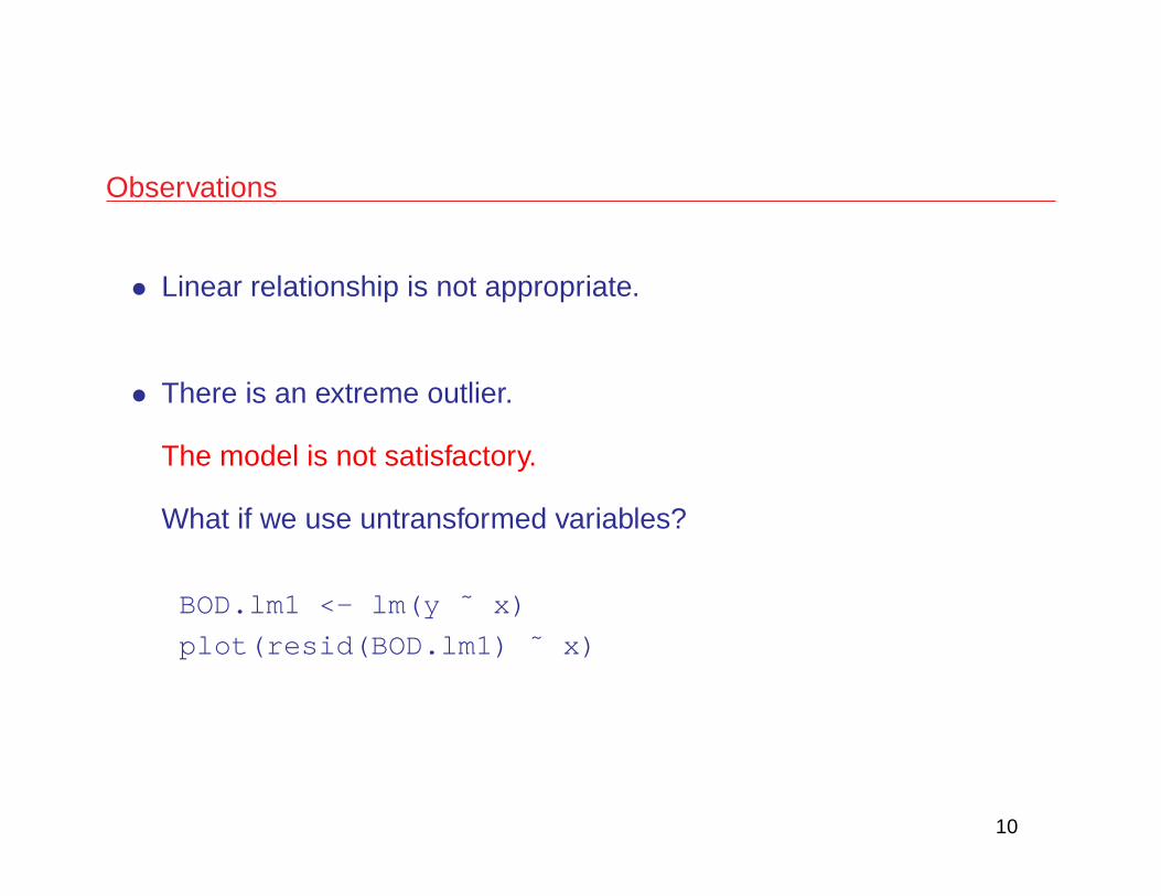
Observations

• Linear relationship is not appropriate.

• There is an extreme outlier.

The model is not satisfactory.

What if we use untransformed variables?

BOD.lm1 <- lm(y ˜ x)

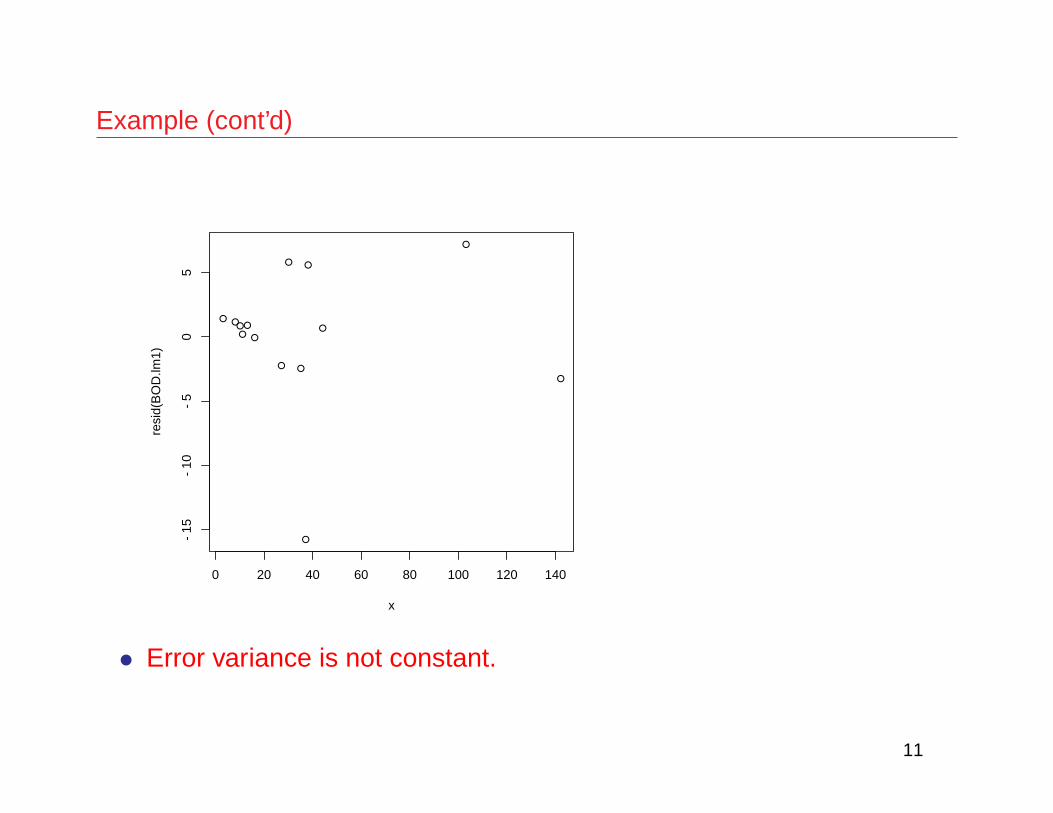
plot(resid(BOD.lm1) ˜ x)

10

Example (cont’d)

● ●●●

●

●

●

●

●

●

●

●

●

●

0 20 40 60 80 100 120 140

−15

−10

−5

05

x

resi

d(B

OD

.lm1)

• Error variance is not constant.

11

Ch. 4.2.4 Partial Regression Plots

• Example: Suppose observations are taken on a response variable y

and three other variables x1, x2 and x3.

• Linear Model:

y = β0 + β1x1 + β2x2 + β3x3 + ε

• One should always check plots of the residuals versus the fittedvalues, and versus each of the predictors.

• An additional way to check whether each predictor should enter theregression model linearly is to look at partial regression plots for eachvariable.

12

Constructing a Partial Regression Plot for x1

• regress y against x2 and x3 (i.e. all variables but x1)

• regress x1 against x2 and x3

• obtain residuals for both regressions

• Plot the y residuals against the x1 residuals

If x1 enters the model linearly, you should see a points scatteredabout a straight line of slope β1. Otherwise, the plot may indicatewhat kind of transformation to apply to x1.

13

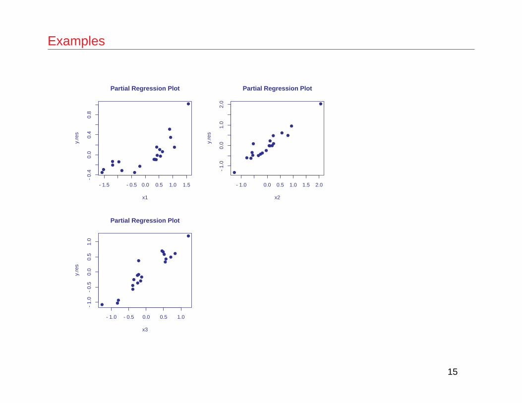
Examples

• Some artificial data is in partial.data : the first three columns arex1, x2 and x3; the last column is y.

partial.plot(partial.data[,-4],partial.data[,4],1) # partial for x1;# the true model is nonlinear# y = .2 exp(x1) + x2 + x3 + e sd(e) = .1partial.plot(partial.data[,-4],partial.data[,4],2) # linear termpartial.plot(partial.data[,-4],partial.data[,4],3) # linear term

14

Examples

●

●

●

●

●●

●●

●●●

●●

●

●

●

●

●

●

●

−1.5 −0.5 0.0 0.5 1.0 1.5

−0.

40.

00.

40.

8Partial Regression Plot

x1

y.re

s

●●

●

●

●

●

●

●●

●●

●

●●

●

●

●

●

●

●

−1.0 0.0 0.5 1.0 1.5 2.0

−1.

00.

01.

02.

0

Partial Regression Plot

x2

y.re

s

●

●

●●

●

●

●

●●

●

●

●

●●

●

●

●

●

●

●

−1.0 −0.5 0.0 0.5 1.0

−1.

0−

0.5

0.0

0.5

1.0


x3

y.re

s

15

Examples

# litters example

partial.plot(litters[,-3],litters[,3],1) # partial for litter size

partial.plot(litters[,-3],litters[,3],2) # partial for body weight

16

Examples

●

●

●

●

●●

●

●

●

●

●

●

●

●

●

●

●

●

●

●

−1.0 −0.5 0.0 0.5 1.0 1.5 2.0

−0.

02−

0.01

0.00

0.01

0.02


lsize

y.re

s

17

Examples

●

●

●

●●

●

●

●

●

●

●

●

●

●

●

●

●

●

●

●

−0.5 0.0 0.5 1.0

−0.

03−

0.02

−0.

010.

000.

010.

020.

03Partial Regression Plot

bodywt

y.re

s

18

•

• Observation: there is mild nonlinearity.

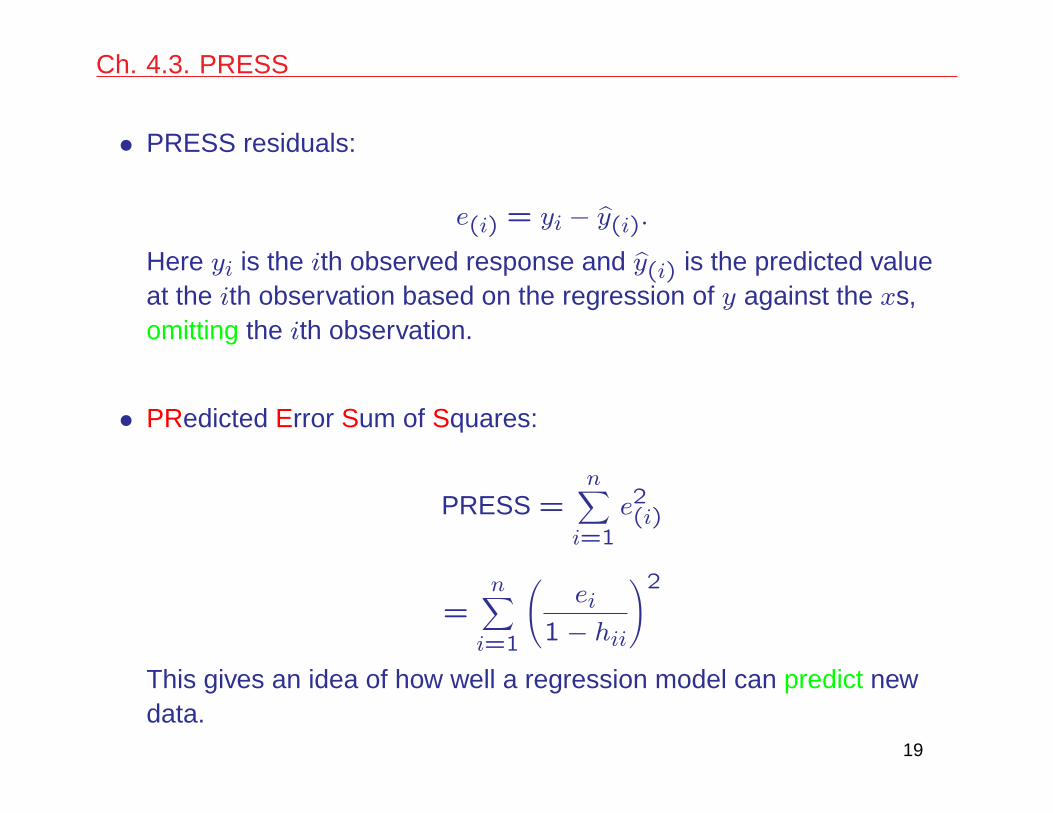
Ch. 4.3. PRESS

• PRESS residuals:

e(i) = yi − y(i).

Here yi is the ith observed response and y(i) is the predicted valueat the ith observation based on the regression of y against the xs,omitting the ith observation.

• PRedicted Error Sum of Squares:

PRESS =n∑

i=1

e2(i)

=n∑

i=1

(ei

1− hii

)2

This gives an idea of how well a regression model can predict newdata.

19

Small values of PRESS are desired.

litters Example

# regression of brain weight against body weight and litter size:> litters.lm <- lm(brainwt ˜ bodywt + lsize, data = litters)

PRESS(litters.lm)[1] 0.0035 # same regression as above, but without the interceptterm:> litters.0 <- lm(brainwt ˜ bodywt + lsize -1, data=litters)> PRESS(litters.0)[1] 0.00482 # regression of brain weight against body weight only,with intercept:> litters.1 <- lm(brainwt ˜ bodywt, data=litters)> PRESS(litters.1)[1] 0.00385 # regression of brain weight against both variablesplus an interaction term:> litters.2 <- lm(brainwt ˜ bodywt + lsize + lsize:bodywt, data=litters)> PRESS(litters.2)[1] 0.0037 # best predictor is the 1st model!

20

Ch. 4.4 Detection and Treatment of Outliers

• An outlier is an extreme observation. If a residual plots more thanabout 3 standard deviation units away from 0, then the observationshould be regarded as an outlier.

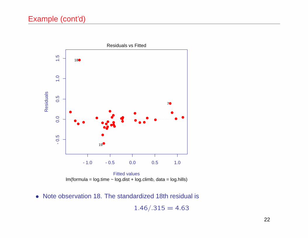
• Detection: Plot residuals vs. fitted values

• Example hills.lm

> hills.lm <- lm(log.time ˜ log.dist + log.climb, data = log.hills)> summary(hills.lm)


(Intercept) -3.1716 0.5350 -5.93 1.3e-06log.dist 0.8944 0.1275 7.02 5.9e-08log.climb 0.1715 0.0932 1.84 0.075

Residual standard error: 0.315 on 32 degrees of freedom....

> plot(hills.lm,pch=16,which=1,col=2)

21

Example (cont’d)

−1.0 −0.5 0.0 0.5 1.0

−0.

50.

00.

51.

01.

5

Fitted values

Res

idua

ls

●●

●

● ●

●

●

●●

● ●●

●

●

●

●●

●

●

●●

● ●

●

●

●●

●

●

●

●

●

●

●

●

lm(formula = log.time ~ log.dist + log.climb, data = log.hills)

Residuals vs Fitted

18

19

7

• Note observation 18. The standardized 18th residual is

1.46/.315 = 4.63

22

• In R:

> resid(hills.lm)[18]/summary(hills.lm)$sigma[1] 4.62

• It is an extreme outlier.

Treatment

• Outlying observations should be examined closely.

• Example cont’d:

> hills[18,]

dist climb time

18 3 350 1.31

• Let’s compare this with the rest of the data:

> summary(hills)

dist climb time

Min. : 2.00 Min. : 300 Min. :0.266

1st Qu.: 4.50 1st Qu.: 725 1st Qu.:0.467

Median : 6.00 Median :1000 Median :0.66223

Mean : 7.53 Mean :1815 Mean :0.965

3rd Qu.: 8.00 3rd Qu.:2200 3rd Qu.:1.144

Max. :28.00 Max. :7500 Max. :3.410

• The 18th race seems to have taken a long time, though it was a shortclimb and a short distance. e.g. Compare this race with the firstobservation:

hills[1,]

dist climb time

1 2.4 650 0.268

This race is shorter but with more climbing. The time is much lessthan for race 18.

• Observation 21 is also comparable for distance and climb, but not atall for time:

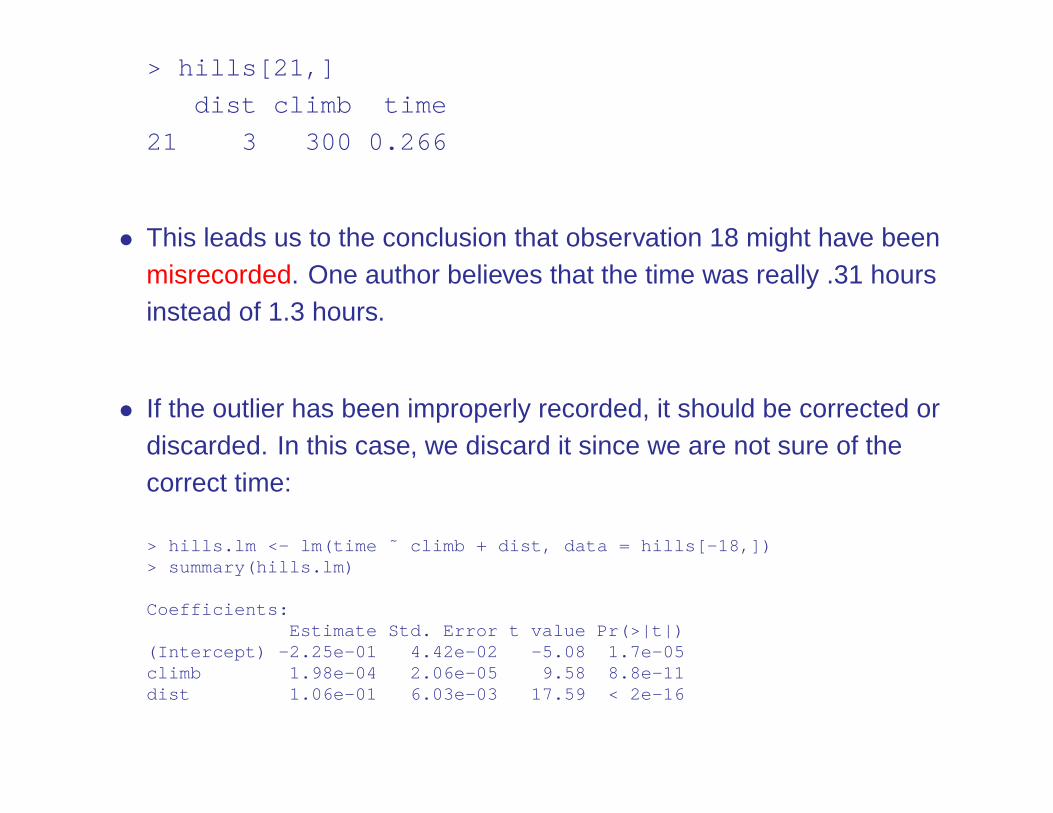
> hills[21,]

dist climb time

21 3 300 0.266

• This leads us to the conclusion that observation 18 might have beenmisrecorded. One author believes that the time was really .31 hoursinstead of 1.3 hours.

• If the outlier has been improperly recorded, it should be corrected ordiscarded. In this case, we discard it since we are not sure of thecorrect time:

> hills.lm <- lm(time ˜ climb + dist, data = hills[-18,])> summary(hills.lm)


(Intercept) -2.25e-01 4.42e-02 -5.08 1.7e-05climb 1.98e-04 2.06e-05 9.58 8.8e-11dist 1.06e-01 6.03e-03 17.59 < 2e-16

Residual standard error: 0.147 on 31 degrees of freedomMultiple R-Squared: 0.972, Adjusted R-squared: 0.97F-statistic: 529 on 2 and 31 DF, p-value: 0

• Note the effect on the standard error after removing that outlier.

Handling Outliers

• If the outlier has not been improperly recorded, then it could meanthat the model is not adequate. In such cases,

– Compare the fitted model with and without the observation.

– If the outlier is making a big difference, one strategy is to reportthe fitted model obtained without the outlier, but to report theoutlier as well. In addition, any plots of the data should properlyidentify the outlying observation.

– Exercise: plot the residuals vs. fitted values for the hills datawithout observation 18. Note that there is now a new outlier. Itcannot be explained away as easily as observation 18.

– Are there other variables that could be included in the model? Acluster of outliers sometimes indicates that an important variablehas been omitted, e.g. gender.

24

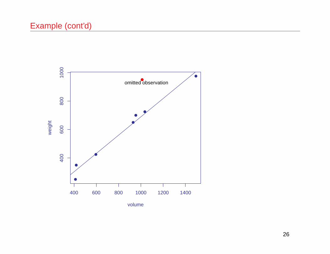
Example – Softbacks

• Observation 6 appears to be an outlier. It has not been recordedincorrectly. It is just different from the other observations. The pagesare of denser material than in the other books; perhaps densityshould be measured and included in the model.

• If we choose to omit this observation, we should do it as follows:

softbacks.lm6 <- lm(weight ˜ volume,

data = softbacks[-6,])

plot(softbacks,pch=16)

abline(softbacks.lm6)

points(softbacks[6,],col=2,pch=16)

text(1050,930,"omitted observation")

25

Example (cont’d)

●

●

●

●

●

●

●

●

400 600 800 1000 1200 1400

400

600

800

1000

volume

wei

ght

●omitted observation

26

The Normal Assumption

• Real data are not likely to be normally distributed.

• For practical purposes, two questions are important:

– How much departure from normality can we tolerate?

– How can we decide if it is plausible that data are from a normaldistribution?

• The first question can be difficult.

– Large departures from normality should be checked for,particularly skewness.

– Small departures can be ignored. For most moderate-sizedsamples, only gross departures will be detectable.

27

What sorts of checks will detect gross departures?

• While histograms have their place, the normal qq plot is moreeffective.

• The following code plots 4 histograms of independent randomsamples of 50 values from a normal distribution.

par(mfrow=c(2,2))

set.seed(2733)

for (i in 1:4) hist(rnorm(50))

par(mfrow=c(1,1))

28

Example - Simulated Normal Data

Histogram of rnorm(50)

rnorm(50)

Fre

quen

cy

−3 −2 −1 0 1 2

02

46

812


rnorm(50)

Fre

quen

cy

−3 −2 −1 0 1 2 3

05

1015

20Histogram of rnorm(50)

rnorm(50)

Fre

quen

cy

−3 −2 −1 0 1 2 3

05

1015


rnorm(50)

Fre

quen

cy

−3 −2 −1 0 1 2 3

05

1015

29

• It is surprising to see how non-normal some of them look!

The normal Q-Q plot

• One sorts the data values.

• These are then plotted against the corresponding values that onemight expect if the data were really from a normal distribution.

• If the data really are from a normal distribution, the plot shouldapproximate a straight line.

par(mfrow=c(2,2))

set.seed(2733) # Use the same samples as before

for(i in 1:4)qqnorm(rnorm(50), main="")

par(mfrow=c(1,1))

30

Example - Simulated Normal Data

●

●

●

●●●

●

●

●

●

●

●

●

●

●

●● ●

●

●

●

●

●

●●

●●

●

●

●

●●

●

●

●

●●

●

●

●

●

●

●

●

●

●

●●

●

●

−2 −1 0 1 2

−3

−2

−1

01

Theoretical Quantiles

Sam

ple

Qua

ntile

s

●

●●

●

●

●

●

●

●

●

●

●

●

●

●

●●

●●

●

●

●

●

●

●

●

●

●

●●

●

●

●

●

●●

●●

●●

●

●

●●

●

●

●●

●

●

−2 −1 0 1 2

−2

−1

01

2


Sam

ple

Qua

ntile

s

●

●

●

●

●

●

●●

●

●

●●

●●

●

●

●

●

●

●●

●

●

● ●●

●

●

●

●●

●

●

●

●

●

●

●

●

●

●

●

●

●

●

●

●

●

●

●

−2 −1 0 1 2

−2

01

2


Sam

ple

Qua

ntile

s

●

●

●

●

●

●

●

●

●

●

●

●

●

●

●

●

●

●

●

●

●

●●

●

●

●

●

●

●●●

●

●●

● ●

●

●●

●

●●

●

●

●

●

●

●

●

●

−2 −1 0 1 2

−2

01

2


Sam

ple

Qua

ntile

s

31

• Simulated plots such as this help train the eye on what to expect insamples of size 50. The process can be repeated several times. Onethen has a standard against which to compare the normal Q-Q plotfor the sample.

Exercise: roller data

• Obtain a normal Q-Q plot of the residuals

roller.lm <- lm(depression ˜ weight,

data = roller)

plot(roller.lm, which=2, pch=16, col=4)

abline(0,1,lwd=2,col=2)

32

Exercise: roller data (cont’d)

●

●

●

●

●

●

●

●

●

●

−1.5 −1.0 −0.5 0.0 0.5 1.0 1.5

−1.

0−

0.5

0.0

0.5

1.0

1.5


Sta

ndar

dize

d re

sidu

als

lm(formula = depression ~ weight, data = roller)

Normal Q−Q plot

10 8

7

33

Setting the sample plot alongside plots for random normal data

par(mfrow=c(2,2))

roller.lm <- lm(depression ˜ weight,

data = roller)

plot(roller.lm, which=2, pch=16, col=4)


for(i in 1:3) {

qqnorm(rnorm(10), pch=16, col=4)


}

par(mfrow=c(1,1))

34

Formal statistical testing for normality

• There are formal statistical tests for normality.

• A difficulty with such tests is that normality is difficult to rule out insmall samples, while in large samples the tests will almost inevitablyidentify departures from normality that are too small to have anypractical consequence for standard forms of statistical analysis.

35

QQ plot for roller data

●

●

●

●

●

●

●

●

●

●

−1.5 −0.5 0.5 1.5

−1.

00.

01.

0


Sta

ndar

dize

d re

sidu

als

Normal Q−Q plot

10 8

7

●●

●

●

●

●

●

●

●

●

−1.5 −0.5 0.5 1.5

−1.

5−

0.5

0.5

Normal Q−Q Plot


Sam

ple

Qua

ntile

s

●

●

●

●●

●

●

● ●

●

−1.5 −0.5 0.5 1.5

−1.

5−

0.5

0.5

Normal Q−Q Plot


Sam

ple

Qua

ntile

s

●

●

●

●

●

●

●●

●

●

−1.5 −0.5 0.5 1.5

−1.

5−

0.5

0.5

Normal Q−Q Plot


Sam

ple

Qua

ntile

s

36

Ch. 4.5.1 Lack of Fit in Simple Regression

• Suppose repeated observations of y are taken at at least one level ofx.

• Example – tomatoes : Electrical conductivity measured at differentsalinity concentrations:

> tomatoessalinity electrical.conductivity

1 1.6 59.52 1.6 53.33 1.6 56.84 1.6 63.15 1.6 58.76 3.8 55.27 3.8 59.18 3.8 52.89 3.8 54.510 6.0 51.711 6.0 48.812 6.0 53.913 6.0 49.014 10.2 44.615 10.2 48.5

37

16 10.2 41.017 10.2 47.318 10.2 46.1

> plot(tomatoes, pch = 16)> tomatoes.lm <- lm(electrical.conductivity˜salinity,

data = tomatoes)> abline(tomatoes.lm)> summary(tomatoes.lm)


(Intercept) 60.67 1.28 47.37 < 2e-16salinity -1.51 0.20 -7.53 1.2e-06

Residual standard error: 2.83 on 16 degrees of freedomMultiple R-Squared: 0.78, Adjusted R-squared: 0.766F-statistic: 56.7 on 1 and 16 DF, p-value: 1.21e-006

●

●

●

●

●

●

●

●

●

●

●

●

●

●

●

●

●

●

2 4 6 8 10

4550

5560

x

y

●

●

●

●

Fitted model:

y = 60.7− 1.51x

with an estimated noise standard error of 2.83.

• How well does this linear model actually fit the data?

• Because of the repeated observations the model can be written as

yij = β0 + β1xi + εij

j = 1,2, . . . , ni, i = 1,2, . . . , m, (n =∑m

i=1 ni).

i.e. There are ni observations at each xi, i = 1,2, . . . , m.

• yi is the ‘best’ estimate of E[y|x = xi]. If we fit a straight line, then yi − yi is ameasure of lack of fit of the linear relationship. Look at the residuals

eij = yij − yi

=yij − yi

pure error+

yi − yi

lack of fit

SSE = SSPE + SSLOF

where

SSPE =m∑

i=1

ni∑j=1

(yij − yi)2

and

SSLOF =m∑

i=1

ni(yi − yi)2

• To test for lack of fit, calculate

F0 =MSLOF

MSPE

• Null hypothesis: E[yi] = β0 + β1xi (i.e. linear model is correct.)

• Degrees of freedom:

– Error: n− 2

– Pure error:∑m

i=1(ni − 1) = n−m

– Lack of fit: n− 2− (n−m) = m− 2.

Therefore, F0 ∼ Fm−2,n−m when the null hypothesis is true. Reject the nullhypothesis when F0 > Fm−2,n−m,α.

> lof.lm(tomatoes.lm)Test of Lack of Fit for Simple Linear Regression

Response: electrical.conductivityDf Sum Sq Mean Sq F value Pr(>F) prediction ratio

Lack of Fit 2 3.5 1.7 0.19 0.8 13.1Pure Error 14 124.5 8.9

litters Example

• brainwt vs. lsize

Here, litter size is replicated so the test can be applied

> litters.0 <- lm(brainwt ˜ lsize, data=litters)> lof.lm(litters.0)Test of Lack of Fit for Simple Linear Regression

Response: brainwtDf Sum Sq Mean Sq F value Pr(>F) prediction ratio


The prediction ratio which is smaller now than for the tomatoes data:

range of fitted values√2MSPE/n

This gives an idea of how well the model is able to predict. Larger values indicatemore predictive power.

38

Example (cont’d)

●

●

●

●

●

●

●

●

●

●

●

●

●

●

●

●

●

●

●

●

4 6 8 10 12

0.38

0.40

0.42

0.44

x

y

●

●

●

●●

●●

●

●

●

39

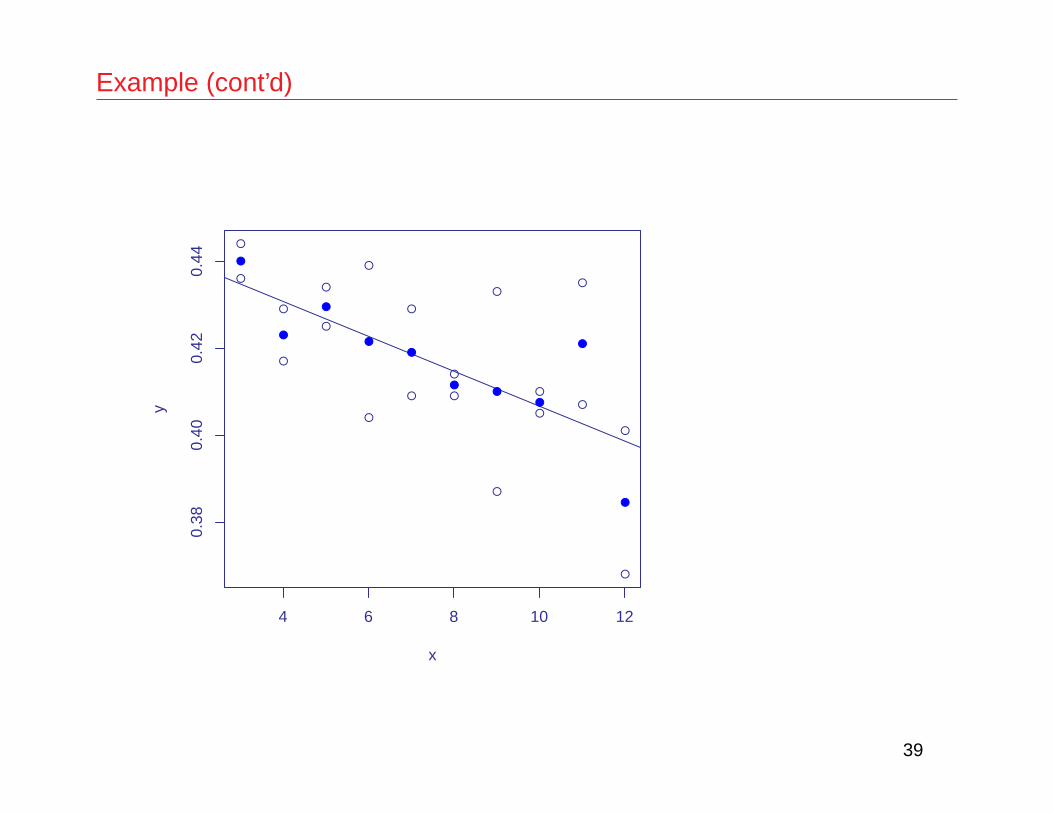
Example (cont’d)

• brainwt vs. bodywt

> litters.1 <- lm(brainwt ˜ bodywt, data=litters)> lof.lm(litters.1)[1] "There are no replicate observations."[1] "Exact Lack of Fit Test is Not Applicable."

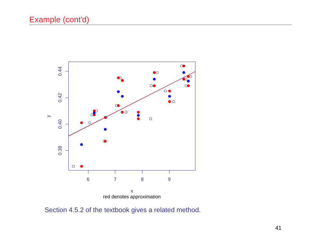
A simple approximation involves averaging neighboring points:

> lof.lm(litters.1,approx=T)The following results are only approximate!!!Test of Lack of Fit for Simple Linear Regression

Response: yDf Sum Sq Mean Sq F value Pr(>F) prediction ratio


40

Example (cont’d)

●

●

●

●

●

●

●

●

●

●

●

●

●

●

●

●

●

●

●

●

6 7 8 9

0.38

0.40

0.42

0.44

x

y

●

●

●

●

●

●

●

●

●

●

●

●

●

●

●

●

●

●

●

●

red denotes approximation

●

●

●

●

●

●

●

●

●

●

Section 4.5.2 of the textbook gives a related method.

41

geophones data

• measurements of the thickness of a subsurface layer in a region ofAlberta.

> geophones.lm <- lm(thickness˜distance,data=geophones)> summary(geophones.lm)


(Intercept) 289.8972 1.9101 151.8 < 2e-16distance -0.4220 0.0362 -11.7 2.2e-16

Residual standard error: 5.6 on 54 degrees of freedomMultiple R-Squared: 0.716, Adjusted R-squared: 0.71F-statistic: 136 on 1 and 54 DF, p-value: 2.22e-016

Fitted model:

y = 289.9− .422x

with a noise standard deviation of 5.6.

> lof.lm(geophones.lm, approx=T)The following results are only approximate!!!Test of Lack of Fit for Simple Linear Regression

42


Lack of Fit 26 1609 62 18.9 8.9e-12 85Pure Error 28 92 3

Example (cont’d)

●●

●

●

●●

●●

●●

●●

●●

●

●●

●

●

●●●

●●●

●●●

●●

●●●

●

●

●● ●

●

●

●

●

●●

●

●

●●●

●●

●

●●

●

●

20 30 40 50 60 70 80

250

255

260

265

270

275

280

x

y

●●

●

●

●●

●●

●●

●●

●●

●

●●

●

●

● ●●

●●●

●●●

●●

●● ●

●

●

● ●●

●

●

●

●

●●

●

●

●● ●

●●

●

●●

●

●


● ●

●

●●

●

●●

●

●

●

●

● ●

● ●

●

●

●

●

●

●

●

● ●

●●

●

43

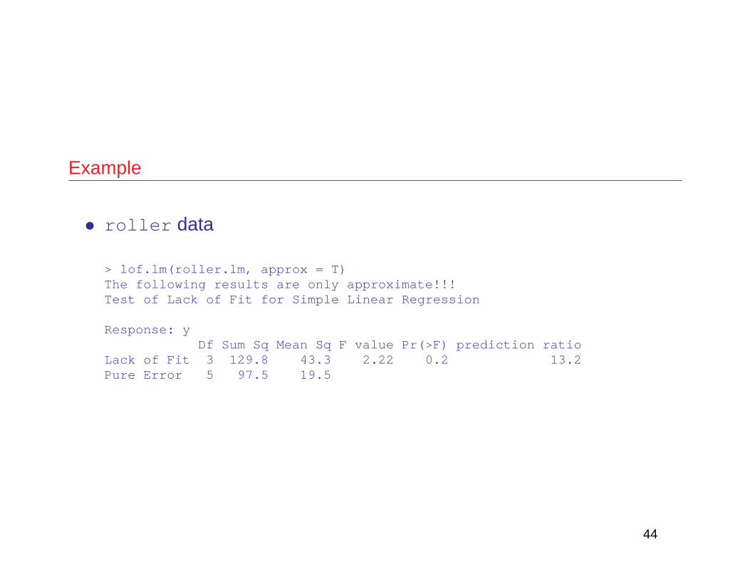
Example

• roller data

> lof.lm(roller.lm, approx = T)The following results are only approximate!!!Test of Lack of Fit for Simple Linear Regression



44

Example (cont’d)

●●

● ●

● ●

●

●

●

●

2 4 6 8 10 12

05

1015

2025

30

x

y

●●

●●

●●

●

●

●

●


●

●

●

●

●

45

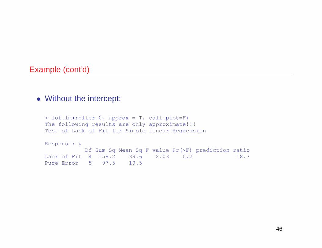
Example (cont’d)

• Without the intercept:

> lof.lm(roller.0, approx = T, call.plot=F)The following results are only approximate!!!Test of Lack of Fit for Simple Linear Regression



46

ch. 4 model adequacy checking - university of british columbia

Documents