ch. 4. the fourier transform

Signals & SystemsProf. M. Song

4.1 Introduction

4.2 The Continuous-Time Fourier Transform4.2.1 Development of the Fourier Transform4.2.2 Existence of the Fourier Transform4.2.3 Examples of the Continuous-Time Fourier Transform

4.3 Properties of the Fourier Transform4.3.1 Linearity4.3.2 Symmetry4.3.3 Time Shifting4.3.4 Time Scaling4.3.5 Differentiation4.3.6 Energy of Aperiodic Signals4.3.7 Convolution4.3.8 Duality4.3.9 Modulation

4.4 Applications of the Fourier Transform4.4.1 Amplitude Modulation4.4.2 Multiplexing4.4.3 The Sampling Theorem4.4.4 Signal Filtering

1

Ch. 4. The Fourier Transform

4.5 Duration Bandwidth Relationships4.5.1 Definitions of Duration and Bandwidth

4.5.2 The Uncertainty Principle

4.6 Summary


2

4.1 Introduction

§ Any periodic signal with period T can be decomposed in terms of harmonics related complex exponential. ð Fourier series

§ Consider the another powerful techniques, called the Fourier transform, for describing both periodic and non-periodic signals for which no Fourier series exists.

• Like the Fourier series coefficients, the Fourier transform specifies the spectral contents of a signal.

• Fourier transform is a valuable tool in the analysis of LTI system.


4.2 The Continuous-Time Fourier Transform (CtFT)

§ Fourier series is restricted to periodic inputs.

§ We will develop a method, the Fourier transform, for representing

aperiodic signals.

3


§ For given , consider the periodic signal

§ Fourier series representation

( ) ( )k

x t x t kT¥

=-¥

= -å%

( )x t ( )x t( )x t%

T ® ¥

[ ]0( ) expnn

x t c jn tw¥

=-¥

= å%

[ ]/ 2

0/ 2

1 ( )expT

n Tc x t jn t dt

Tw

-= -ò %

( )x t ( )x t%

4

4.2.1 Development of the Fourier Transform


• When ,T ® ¥

0 02 2, , ( ) ( )nd n x t x tT Tp pw w w w= ® = ® ®%

[ ]( ) ( )expX x t j t dtw w¥

-¥= -ò

[ ]( )exp2n t

dc x t j t dtw wp

¥

=-¥= -ò

( ) [ ] [ ]( )exp exp2t

dx t x t j t dt j tw

ww wp

¥ ¥

=-¥ =-¥

é ù= -ê úë ûò ò

[ ]0( ) expnn

x t c jn tw¥

=-¥

= å% [ ]/ 2

0/ 2

1 ( )expT

n Tc x t jn t dt

Tw

-= -ò %

( )X w

( ) ( ) [ ]1 X exp2

x t j t dw

w w wp

¥

=-¥= ò

Fourier Transform PairFourier Transform Pair


§ Fourier transform• Analysis equation

• Synthesis equation

• Notation

§ Spectrum

• Magnitude spectrum :

• Phase spectrum :

• Energy spectrum :

[ ]( ) ( )expX x t j t dtw w¥

-¥= -ò

[ ]1( ) ( )exp2

x t X j t dw w wp

¥

-¥= ò

{ } { }1( ) ( ), ( ) ( ) , ( ) ( )x t X X x t x t Xw w w-« = =F F

[ ]( ) ( ) exp ( )X X jw w f w=

( )X w

( ), ( )X w f wR2( )X w

6

* An aperiodic signal has a continuous spectrum rather than a line spectrum.


§ Fourier transform exists if x(t) is absolutely integrable.

• x(t) is energy signal if x(t) is absolutely integrable.

ð Energy signal has Fourier transform.

• Being absolutely integrable is a sufficient condition.− Power signals (unit-step signal, periodic signal) have Fourier

transforms.

− They are not absolutely integrable.

( )x t dt¥

-¥< ¥ò

4.2.2 Existence of the Fourier Transform

7


Rectangular pulse

§ Rectangular pulse ⇔ Sinc function

( ) rect tx tt

æ ö= ç ÷è ø

[ ] [ ]/ 2

/ 2

2( ) ( )exp exp sin2

X x t j t dt j t dtt

t

wtw w ww

¥

-¥ -= - = - =ò ò

( )x t

2t

2t

-

Ex. 4.2.1Ex. 4.2.1

4.2.3 Examples of the Continuous-Time Fourier Transform

8


Triangular pulse

| |1 , | |( )

0, | |

t ttx tt

tt

t t

ì - £ïæ ö= D = íç ÷è ø ï >î

[ ] 2 2

0( ) exp 2 1 cos sinc Sa

2 2t tX j t dt t dt

t wt wtw w w tt t p

¥

-¥

æ ö æ ö= D - = - = =ç ÷ ç ÷è ø è øò ò

2 2sinc Sa2 2

t wt wttt p

æ öD « =ç ÷è ø

0t

x(t)

Ex. 4.2.2Ex. 4.2.2

9


One-sided exponential signal

[ ]( ) exp ( )x t t u ta= -

[ ] [ ]

[ ]

[ ]0

0

( ) exp ( )exp

exp ( )

1 exp ( )( )

1

X t u t j t dt

j t dt

j tj

j

w a w

a w

a wa w

a w

¥

-¥

¥

¥

= - -

= - +

é ù= - +ë û- +

=+

òò

Ex. 4.2.3Ex. 4.2.3

10


Two-sided exponential signal

[ ]( ) exp | | , 0x t ta a= - >

[ ] [ ] [ ] [ ]

[ ] [ ]

0

00

0

2 2

( ) exp exp exp exp

exp ( ) exp ( )

1 1 2

X t j t dt t j t dt

j t dt j t dt

j j

w a w a w

a w a w

aa w a w a w

¥

-¥

¥

-¥

= - + - -

= - + - +

= + =- + +

ò òò ò

Ex. 4.2.4Ex. 4.2.4

11


Impulse function

§ Impulse signal consists of equal-amplitude sinusoids of all frequency.

{ } [ ]( ) ( )exp 1t t j t dtd d w¥

-¥= - =òF

( ) 1td «

[ ]1( ) exp2

t j t dd w wp

¥

-¥= ò

{ } [ ]1 1exp 2 ( )j t dtw pd w¥

-¥= - =òF

1 2 ( )pd w«

[ ]11 2 ( )exp2

j t dpd w w wp

¥

-¥= ò

Ex. 4.2.5Ex. 4.2.5

12


§ behaves like as an impulse at t=0

[ ]1 exp ( ) (0)2

j t d g t dt gw wp

¥ ¥

-¥ -¥

é ù Þê úë ûò ò

[ ] [ ]1 1exp ( ) ( )exp ( )2 2

1 ( )2

j t d g t dt g t j t dt d

G d

w w w wp p

w wp

¥ ¥ ¥ ¥

-¥ -¥ -¥ -¥

¥

-¥

é ù é ù= - -ê ú ê úë ûë û

= -

ò ò ò ò

ò

[ ]0

1 1 1( ) ( ) ( )exp (0)2 2 2 t

G d G d G j t d gw w w w w w wp p p

¥ ¥ ¥

-¥ -¥ -¥=

- = = =ò ò ò

[ ]1( ) exp2

t j t dd w wp

¥

-¥\ = ò

[ ](1/ 2 ) exp j t dp w w¥

-¥ò

Ex. 4.2.6Ex. 4.2.6

13


§ Exchange t and w in Eq. (4.2.11)

[ ] [ ]1 1( ) exp ( ) exp2 2

t j t d jt dtd w w d w wp p

¥ ¥

-¥ -¥= Þ =ò ò

[ ]2 ( ) 1exp 2 ( )j t dtpd w w pd w¥

-¥- = - =ò

1 2 ( )pd w«

Ex. 4.2.6Ex. 4.2.6

14


§ In Example 4.2.1

§ As , and

2( ) rect( / ) ( ) sin2

x t t X wtt ww

= « =

2lim sin 2 ( )2t

wt pd ww®¥

=

, ( ) 1x tt ® ¥ ® ( ) 2 ( )X w pd w®

Ex. 4.2.7Ex. 4.2.7

15


Exponential signal

[ ]0( ) expx t j tw=

[ ] [ ]

[ ]0

0

0

( ) exp exp

exp ( )

2 ( )

X j t j t dt

j t dt

w w w

w w

pd w w

¥

-¥

¥

-¥

= -

= - -

= -

òò

[ ]0 0exp 2 ( )j tw pd w w« -

Ex. 4.2.8Ex. 4.2.8

16


§ Fourier transform of a periodic signal• Periodic signal is a power signal.

• Its Fourier transform contains impulses.

• Its Fourier transform can be obtained from the Fourier series coefficients.

17


Periodic signal

§ Fourier series representation

§ Fourier transform

§ The Fourier transform of a periodic signal is an impulse train with impulses located at , each of which has a strength , and all impulses are separated from each other by .

02( ) ( ),x t x t TTpw= + =

[ ]0( ) expnn

x t c jn tw¥

=-¥

= å

[ ]{ }0 0( ) exp 2 ( )n nn n

X c jn t c nw w p d w w¥ ¥

=-¥ =-¥

= = -å åF

0nw w= 2 ncp

0w

Ex. 4.2.9Ex. 4.2.9

18


Impulse train

§ Fourier series coefficients

§ Fourier transform

( ) ( )n

x t t nTd¥

=-¥

= -å

1 2 1 2 1( )exp ( )expn T T

nt ntc x t j dt t j dtT T T T T

p pd< > < >

é ù é ù= - = - =ê ú ê úë û ë ûò ò1 2( ) exp

n

ntx t jT T

p¥

=-¥

é ù= ê úë ûå

2 2exp 2nt njT Tp ppd wé ù æ ö« -ç ÷ê úë û è ø

1 2 2 2expn n

nt njT T T T

p p pd w¥ ¥

=-¥ =-¥

é ù æ ö« -ç ÷ê úë û è øå å

2 2( )n

nXT Tp pw d w

¥

=-¥

æ ö= -ç ÷è ø

åImpulse

train

Ex. 4.2.10Ex. 4.2.10

19


§ If,

then 1 1 2 2( ) ( ), ( ) ( )x t X x t Xw w« «

1 2 1 2( ) ( ) ( ) ( )ax t bx t aX bXw w+ « +

4.3.1 Linearity

4.3 Properties of the Fourier Transform

20

§ Several useful properties of the Fourier transform allow some problems to be solved almost by inspection.


Sinusoidal signal

[ ] [ ]{ }1 0 0 01( ) cos exp exp2

x t t j t j tw w w= = + -

[ ] [ ]{ }2 0 0 01( ) sin exp exp

2x t t j t j t

jw w w= = - -

{ }2 0 0( ) ( ) ( )Xjpw d w w d w w= - - +

1 0( ) cosx t tw=

2 0( ) sinx t tw=

{ }1 0 0( ) ( ) ( )X w p d w w d w w= - + +

[ ][ ]

0 0

0 0

exp 2 ( )

exp 2 ( )

j t

j t

w pd w w

w pd w w

« -

- « +

Ex. 4.3.1Ex. 4.3.1

21


§ If x(t) is a real-valued time signal, then

<Proof>

§ The magnitude is an even function and the phase is an odd function.

*( ) ( )X Xw w- =

[ ]

[ ]{ }

[ ]{ }

*

*

*

( ) ( )exp ( )

( ) exp ( )

( )exp

( )

X x t j t dt

x t j t dt

x t j t dt

X

w w

w

w

w

¥

-¥

¥

-¥

¥

-¥

- = - -

= -

= -

=

òò

ò

[ ]( ) ( ) exp ( )X X jw w f w=

4.3.2 Symmetry

22[ ]*( ) ( ) exp ( )X X jw w f w= -

[ ]( ) ( ) exp ( ) ( ) ( ) , ( ) ( )X X j X Xw w f w w w f w f w- = - - Þ = - - = -


Real signal

[ ]

[ ] [ ]

[ ] [ ]

[ ] [ ] [ ] [ ]

{ }

0

0

0 0

0 0

1( ) ( )exp21 1( )exp ( )exp

2 21 1( )exp ( )exp

2 21 1( ) exp ( ) exp ( ) exp ( ) exp

2 2

set

1 ( ) exp ( ) exp2

x t X j t d

X j t d X j t d

X j t d X j t d

X j j t d X j j t d

X j t j t

w w wp

w w w w w wp p

q q q w w wp p

w f w w w w f w w wp p

w w f w w

w q

p

¥

-¥

¥

-¥

¥ ¥

¥ ¥

=

= +

= - - +

= - - +

é ù= + + - +

¬ -

û

=

ë

ò

ò ò

ò ò

ò ò

{ }( )

{ }

0

0

( )

1 2 ( ) cos ( )2

d

X t d

f w w

w w f w wp

¥

¥

é ùë û

= +

ò

ò

Ex. 4.3.2Ex. 4.3.2

23


Even and real-valued signal

[ ]

( )

0

( ) ( ) exp

( ) cos sin

( ) cos ( )sin

2 ( )cos

X x t j t dt

x t t j t dt

x t t dt j x t t dt

x t t dt

w w

w w

w w

w

¥

-¥

¥

-¥

¥ ¥

-¥ -¥

¥

= -

= -

= -

=

òòò òò

Ex. 4.3.3Ex. 4.3.3

24


§ If

then,

<Proof>

( ) ( )x t X w«

[ ]0 0( ) ( )expx t t X j tw w- « -

[ ]0 0( )exp ( )x t j t Xw w w« -

[ ] [ ]

[ ] [ ][ ]

0

0

0

00 set( )exp ( )exp ( )

exp ( )exp

ex

p ( )

tx t t j t dt x j t d

j t x j d

X

t

j t

w t w t t

w t wt

t

t

w w

¥ ¥

-¥ -¥

¥

-¥

- - = - +

=

¬ = -

- -

= -

ò òò

[ ] [ ] ( ) ( )0 0 0( )exp exp ( )expx t j t j t dt x t j t d Xw w w w t w w¥ ¥

-¥ -¥é ù- = - - = -ë ûò ò

Amplitude isnot changed

AM modulation

4.3.3 Time Shifting

25


§ If

then,( ) ( )x t X w«

1( )x t X waa a

æ ö« ç ÷è ø

0 00

0

0t

0

0

0

t

t

2 0

0/2

2 0

0/2

t0 t0

t0/2 t0/2

2t0 2t0

X

X

X

x t

x t

x t/2

4.3.4 Time Scaling

26


( ) rect , 0tx t aa at

æ ö= >ç ÷è ø

rect sinc rect sinc2 2

t twt a wtt a tt p t pa

ì ü ì üæ ö æ ö= Þ =í ý í ýç ÷ ç ÷è ø è øî þ î þ

F F

Ex. 4.3.4Ex. 4.3.4

27


§ If,

then

<Proof>

( ) ( )x t X w«

( ) ( )( ), ( ) ( )n

nn

dx t d x tj X j Xdt dt

w w w w« «

[ ]1( ) ( )exp2

x t X j t dw w wp

¥

-¥= ò

[ ] { }1( ) 1 ( ) exp ( )2

dx t X j j t d j Xdt

w w w w w wp

¥ -

-¥= =ò F

4.3.5 Differentiation

28


§ Integration

§ Problems• Differentiation operation destroys any dc component of y(t).

• X(0) must be zero. (See 166 page, )

§ When , we add a dc term , where c depends on the

average of x(t),

1( ) ( ) ( )t

y t x d Xj

t t ww-¥

= «ò( ) 1( ) ( ) ( ) ( ) ( ) ( ) ( )

t dy ty t x d x t X j Y Y Xdt j

t t w w w w ww-¥

= Þ = « = Þ =ò

(0) ( ) 0X x dt t¥

-¥= =ò

1( ) ( ) ( ) ( ) (0) ( )t

y t x d Y X Xj

t t w w p d ww-¥

= « = +ò

( ) (0)y X¥ =

(0) 0X ¹ ( )cd w

(0)c Xp=

29


Unit step function

§ Signum function

• sgnt has a zero dc component

§ Unit step function

1, 0sgn 0, 0

1, 0

tt t

t

- <ìï= =íï >î

sgn 2 ( ) sgn 2 ( )td t t t d

dtd d t t

-¥= Þ = ò

{ } { }1 2sgn 2 ( )t tj j

dw w

= =F F

1 1( ) sgn2 2

u t t= +

{ } { }1 1 1( ) sgn ( )2 2

u t tj

pd ww

ì ü= + = +í ýî þ

F F F

Ex. 4.3.5Ex. 4.3.5

30


§ Parseval's theorem

§ Parseval's relation for aperiodic signals.

<Proof>

2 21 ( ) nTn

x t dt cT

¥

< >=-¥

= åò

2 21( ) ( )2

E x t dt X dw wp

¥ ¥

-¥ -¥= =ò ò

[ ]

[ ]{ }

2 *

*

*

2

( ) ( ) ( )

1( ) ( )exp2

1 ( ) ( )exp21 ( )

2

E x t dt x t x t dt

x t X j t d dt

X x t j t dt d

X d

w w wp

w w wp

w wp

¥ ¥

-¥ -¥

¥ ¥

-¥ -¥

¥ ¥

-¥ -¥

¥

-¥

= =

ì ü= -í ýî þ

= -

=

ò ò

ò ò

ò ò

ò

4.3.6 Energy of aperiodic signals

31


§ Energy density spectrum

• Energy in the frequency band

§ Power density spectrum• Let x(t) be a power signal and define as

2( )( ) ( )

2X

E dw

w w wp

¥

-¥= Þ = òE E

1 2w w w£ £

2

1

( )E dw

ww wD = ò E

( )x tt

( ),( )

0, otherwisex t t

x tt

t t- < <ì= í

î

32


• The average power of x(t)

• Power density spectrum, power spectrum density (PSD)

⇒ PSD depends only on the magnitude of the spectrum.

221 1lim ( ) lim ( )2 2

P x t dt x t dtt

ttt tt t¥

- -¥®¥ ®¥

é ù é ù= =ê ú ê úë û ë ûò ò2

2

1 1lim ( )2 2

( )1 lim2 2

1 ( )2

P X d

Xd

S d

tt

t

t

w wt p

ww

p t

w wp

¥

-¥®¥

¥

-¥ ®¥

¥

-¥

é ùì ü= í ýê úî þë ûé ù

= ê úê úë û

=

ò

ò

ò

2( )( ) lim

2X

S t

t

ww

t®¥

é ù= ê ú

ê úë û

33


§ One-sided exponential signal

§ Energy density spectrum

§ Total energy

§ Energy in

⇒84.4 % of total energy

[ ]( ) exp ( )x t t u t= -

2

2

( ) 1 1 1( )1

( )2 2 1

XX

jw

ww

wp p w

= =+

¬ =+

E

2

1 1 1( )2 21

E d dw w wp w

¥ ¥

-¥ -¥= = =

+ò òE

12 2 2

1 1 1tan ,1

xdx C da ax a

w pw

¥-

-¥

ì ü= + =í ý+ +î þò òQ

( )4 4 1 124 0

1 1 1( ) 2 tan 4 tan 0 0.42202 1

E d dw w wp pw

- -

-D = = = - »

+ò òE

Ex. 4.3.6Ex. 4.3.6

34


§ If

then

<Proof>

( ) ( ), ( ) ( )x t X h t Hw w« «

( ) ( ) ( ) ( ) ( ) ( )y t x t h t Y X Hw w w= * « =

{ } [ ]

[ ]

[ ]

[ ]

( ) ( ) ( ) ( ) exp

( ) ( ) exp

( ) ( ) exp

( )exp ( )

( ) ( )

x t h t x t h t j t dt

x h t d j t dt

x h t j t dt d

x j H d

X H

w

t t t w

t t w t

t wt w t

w w

¥

-¥

¥ ¥

-¥ -¥

¥ ¥

-¥ -¥

¥

-¥

* = * -

é ù= - -ê úë ûé ù= - -ê úë û

= -

=

ò

ò ò

ò ò

ò

F

4.3.7 Convolution

35


§ Amplitude and phase spectrum of output signal

§ Hence, convolution in the time domain is equivalent to multiplication in the frequency domain, which, in many cases, is convenient and can be done by inspection.

( ) ( ) ( )Y X Hw w w=

( ) ( ) ( )Y X Hw w w= +R R R

36


LTI system[ ]( ) ( ), ( ) exp ( ) ( ) ??x t u t h t at u t y t= = - Þ =

1 1( ) ( ) , ( )X Hj j a

w pd w ww w

= + =+

{ } [ ]{ }

1 1( ) ( )

1( )( )

1 1 1( )

1 1 1 1( )

1 1( ) exp ( )

Yj j a

a j j a

a a j j a

a j a j a

u t at u ta a

w pd ww w

p d ww w

p d ww w

pd ww w

é ù é ù= +ê ú ê ú+ë û ë û

= ++

é ù= + -ê ú+ë û

é ù= + -ê ú +ë û

= - -F F

[ ]{ }1( ) 1 exp ( )y t at u ta

\ = - -

Ex. 4.3.7Ex. 4.3.7

37


Triangle signal

1( ) , ( ) rectt tz t x tt tt

æ ö æ ö= D =ç ÷ ç ÷è ø è ø

1( ) sinc2

X wtwt

=

2 22 1 1( ) ( ) sinc sinc

2 2Z X wt wtw w

ttæ ö æ ö= = = ç ÷ç ÷ è øè ø

( ) ( ) ( ) ( ) ??z t x t x t Z w= * Þ =

Ex. 4.3.8Ex. 4.3.8

38


LTI system

[ ] [ ] [ ]{ }( ) exp ( ), ( ) exp exp ( ) ( ) ??h t at u t y t bt ct u t x t= - = - - - Þ =

1( )Hj a

ww

=+

1 1( )Yj b j c

ww w

= -+ +

( )( )( )

1 1

Y j a j aXH j b j c

a b a c a b a cj b j c j b j c

w w www w w

w w w w

+ += = -

+ +- - - -

= + - - = -+ + + +

[ ] [ ]( ) ( ) exp ( ) ( ) exp ( )x t a b bt u t a c ct u t\ = - - - - -

Ex. 4.3.9Ex. 4.3.9

39


Integration

( ) ( ) ( ) ( )t

y t x d x t u tt t-¥

= = *ò1( ) ( )Uj

w pd ww

= +

1 ( )( ) ( ) ( ) ( ) ( ) (0) ( ) XY X U X Xj j

ww w w w pd w p d ww w

é ù= = + = +ê ú

ë û

Ex. 4.3.10Ex. 4.3.10

40


§ Energy spectrum density of the response of an LTI system

• The phase characteristics of the system does not affect the energy

spectrum density of the output.

2 2 2 2( ) ( ) ( ) ( ) ( )Y X H X Hw w w w w= =

41


§ If

then

<Proof>

( ) ( )x t X w«

( ) 2 ( )X t xp w« -

{ } [ ]

[ ]

( ) ( ) exp

12 ( )exp ( )2

2 ( )

X t X t j t dt

X t jt dt

x

w

p wp

p w

¥

-¥

¥

-¥

= -

é ù= -ê úë û= -

ò

ò

F

4.3.8 Duality

42


§ Time limiting and frequency limiting are mutually exclusive.• If x(t) is time limited, then X(w) is never band limited.

• If X(w) is band limited, then x(t) is never time limited.

rect sinc2

t twtt p

«

2sinc rect2

B

B B

tw p wp w w

«

Ex. 4.3.11Ex. 4.3.11

43


[ ]( ) ( ) expX x t j t dtw w¥

-¥= -ò

[ ] { }( ) ( )( ) exp ( ) ( )dX x t jt j t dt jt x td

w ww

¥

-¥= - - = -ò F

( )( ) ( ) dXjt x td

ww

\ - «

( )( ) ( )n

nn

d Xjt x td

ww

\ - «

Ex. 4.3.12Ex. 4.3.12

44


§ If,

then

( ) ( ), ( ) ( )]x t X m t Mw w« «

[ ]1 1( ) ( ) ( ) ( ) ( ) ( )2 2

x t m t X M X M dw w s w s sp p

¥

-¥« * = -ò

{ } [ ]

[ ] [ ]

[ ]

[ ]

( ) ( ) ( ) ( ) exp

1 ( )exp ( )exp2

1 ( ) ( ) exp ( )21 ( ) ( )

21 ( ) ( )

2

x t m t x t m t j t dt

X j t d m t j t dt

X m t j dt d

X M d

X M

w

s s s wp

s w s sp

w w s sp

w wp

¥

-¥

¥ ¥

-¥ -¥

¥ ¥

-¥ -¥

¥

-¥

= -

é ù= -ê úë û

é ù= - -ê úë û

= -

= *

ò

ò ò

ò ò

ò

F

4.3.9 Modulation

45


§ AM modulation

( ) ( )x t X w«

[ ]0 0 01( )cos ( ) ( )2

x t X Xw w w w w« - + +

46


Sampling signal

§ Periodic impulse train

§ Sampled signal

2 2( ) ( ) ( )n n

np t t nT PT Tp pd w d w

¥ ¥

=-¥ =-¥

æ ö= - « = -ç ÷è ø

å å

( ) ( ) ( )sx t x t p t=

[ ]1( ) ( ) ( )21 2( )

1 2

s

n

n

X X P

nXT T

nXT T

w w wp

pw d w

pw

¥

=-¥

¥

=-¥

= *

æ ö= * -ç ÷è ø

æ ö= -ç ÷è ø

å

å

Ex. 4.3.13Ex. 4.3.13

47


§ consists of a periodically repeated replica of

2Tp 4

Tp2

Tp

-4Tp

-

1T

( )sX w ( )X w

48

Ex. 4.3.13Ex. 4.3.13


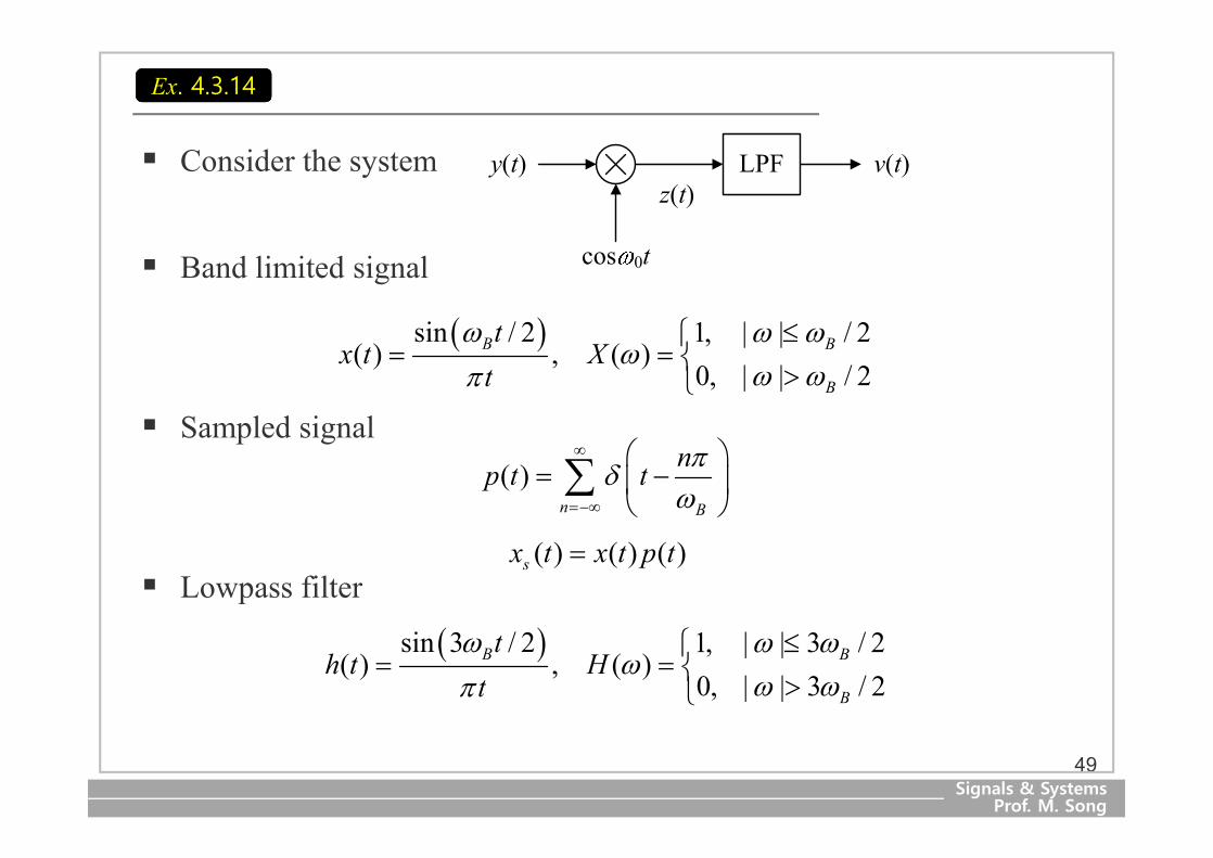
§ Consider the system

§ Band limited signal

§ Sampled signal

§ Lowpass filter

LPFy(t)

cos 0t

v(t)z(t)

( )sin / 2 1, | | / 2( ) , ( )

0, | | / 2B B

B

tx t X

tw w w

ww wp

£ì= = í >î

( )n B

np t t pdw

¥

=-¥

æ ö= -ç ÷

è øå

( ) ( ) ( )sx t x t p t=

( )sin 3 / 2 1, | | 3 / 2( ) , ( )

0, | | 3 / 2B B

B

th t H

tw w w

ww wp

£ì= = í >î

Ex. 4.3.14Ex. 4.3.14

49


§ Output signal

§ Spectra

0

0

1

Z(

BB

H(

0

X(

1

B/2B/2

0

Y(

1

B/2B/2

3 B/2-3 B/2

( ) ( ) ( )sy t x t h t= *

( ) ( ) ( ) ( )Y X H Xw w w w= =

50

Ex. 4.3.14Ex. 4.3.14


§ Power spectrum of the periodic signal x(t) with period T

• where cn are the Fourier series coefficients of x(t)

§ Define the truncated signal

§ Fourier transform of periodic signal x(t)

( )20 0

2( ) 2 ,nn

S c nTpw p d w w w

¥

=-¥

= - =å

( ) ( )rect2tx t x tt t

æ ö= ç ÷è ø

[ ]1 1( ) 2 Sa ( ) ( ) 2 Sa ( ) ( )2 2

X X X dt w t wt w t qt w q qp p

¥

-¥= * = -ò

0( ) 2 ( )nn

X cw p d w w¥

=-¥

= -å

Ex. 4.3.15Ex. 4.3.15

51


§ Average power of

§ Power spectrum of x(t)

( ) ( )2

*0 0

( )2 Sa Sa

2 n mn m

Xc c n mt w

t w w t w w tt

¥ ¥

=-¥ =-¥

é ù é ù= - -ë û ë ûå å

( ) ( )0 0

1,0,

m nn m

m nd w w d w w

=ì- - = í ¹î

( )x tt

( )2

20

( )( ) lim 2

2 nn

XS c nt

t

ww p d w w

t

¥

®¥=-¥

\ = = -å

52

Ex. 4.3.15Ex. 4.3.15


§ Modulation• Modulated signal

where m(t) is a carrier signal.0( ) ( ) ( ) ( )cosy t x t m t x t tw= =

4.4.1 Amplitude Modulation

53

4.4 Applications of the Fourier Transform

Signal multiplier

• Spectrum[ ]

[ ]

0 0

0 0

1( ) ( ) ( ) ( )21 ( ) ( )2

Y X

X X

w w p d w w d w wp

w w w w

= * - + +

= - + +

Shift in frequency


54

[ ]0 01( ) ( ) ( )2

Y X Xw w w w w= - + +

§ This process of shifting the spectrum of the signal by w0 is necessary because low-frequency (baseband) information signals cannot be propagated easily be radio waves.


§ Process of extracting the information from the modulated signal

§ Synchronous demodulation• Demodulated signal

• Low-pass filtering [Fig. 4.4.3]

LPFy(t)

cos 0t

v(t)z(t)

0( ) ( )cosz t y t tw=

[ ]0 0

0 0

1( ) ( ) ( )21 1 1( ) ( 2 ) ( 2 )2 4 4

Z Y Y

X X X

w w w w w

w w w w w

= - + +

= + - + +

2, | |( )

0, | |B

B

Hw w

ww w

£ì= í >î

( ) ( ) ( ) ( )V H Z Xw w w w= =

55

Demodulation


• Spectrum of the demodulated output

56

LPFy(t)

cos 0t

v(t)z(t)


§ Frequency Division Multiplexing (FDM): A very useful technique for

simultaneously transmitting several information signals by assigning

a portion of the final frequency to each signal

• Examples− AM radio stations− TV stations− Fire engines− Police cruisers− Taxicabs− Mobile phones− And many other sources of radio waves

4.4.2 Multiplexing

57


§ Frequency division multiplexing (FDM)• Modulated signal

• Spectrum

1 1 2 2 3 3( ) ( )cos ( )cos ( )cosy t x t t x t t x t tw w w= + +

[ ] [ ]

[ ]

1 1 1 1 2 2 2 2

3 3 3 3

1 1( ) ( ) ( ) ( ) ( )2 2

1 ( ) ( )2

Y X X X X

X X

w w w w w w w w w

w w w w

= - + + + - + +

+ - + +

0

1

0

1

0

1

B1 B1 B2 B3 B3B2

4.4.2 Multiplexing

58


§ FDM system

59


§ The sampling theorem has the most impact on information

transmission and processing.

§ Sampling process• Let x(t) be a band limited signal.

• Sampler output, sampled signal

where p(t) is the periodic impulse train

− T : sampling period

− : sampling frequency

( ) 0, for | | BX w w w= >

( ) ( ) ( )sx t x t p t=

( ) ( )n

p t t nTd¥

=-¥

= -å

2 /s Tw p=

4.4.3 The Sampling Theorem

60


§ Spectrum of sampled signal

( )2 2 2( ) sn n

nP nT T Tp p pw d w d w w

¥ ¥

=-¥ =-¥

æ ö= - = -ç ÷è ø

å å1 1 1( ) ( ) ( ) ( ) ( ) ( )

2 2s sn

X X P X P d X nT

w w w s w s s w wp p

¥¥

-¥=-¥

= * = - = -åò

61


§ If , x(t) can be recovered from xs(t) using LPF.

§ If , x(t) cannot be recovered from xs(t). ⇒ aliasing

§ Nyquist sampling rate

2s Bw w³

2s Bw w<

2s Bw w=

|Xs

BB 0ss

s+ Bs Bs+ Bs B

BB 0 ss

BB 0 ss ss

|Xs

|Xs

s > 2 B

s < 2 B

s = 2 B

62

Nyquist sampling theorem


Nyquist sampling rate

§ Band limited signal with

§ Nyquist sampling rate

§ Sampling period

5 kHzBf =

2 10 kHzs Bf f= =

42 2 (2 5000) 2 10 rad/secs Bw w p p= = ´ ´ = ´

1 2 0.1 mss s

Tf

pw

= = =

Ex. 4.4.1Ex. 4.4.1

63


Aliasing

§ Band limited signal with

§ Sampling rate is

§ Aliasing

5 kHzBf =

8 kHzsf =

( )2s Bf f£Q

Ex. 4.4.2Ex. 4.4.2

64


Sampling of modulated signal

§ xa(t) is band limited to the range

§ Modulated signal xm(t)

§ Filtered signal xb(t) with LPF of

§ Sampled signal xs(t) with

800 1200 Hzf£ £

200 Hzcw =

1/ 400 sec, 400 HzsT f< >

1/ 500 sec, 500 HzsT f= =

Ex. 4.4.3Ex. 4.4.3

65


§ Spectra

• we can recover xa(t) from xs(t) by using a BPF

Xa

0 1 1.20.8-1

1

-1.2 -0.8

Xm

0 1-1

1

2-2

Xb

0 1-1

1

2-2

Xs

0 1-1

500

2-2

66

Ex. 4.4.3Ex. 4.4.3


§ Reconstruction• We can recover x(t) from sampled signal xs(t) by using a LPF

• Reconstructed signal

• It can be interpreted as using interpolation to reconstruct x(t) from its

samples x(nT) .

( ) ( ) ( )sX H Xw w w=

1, | | sin( ) , ( )0, | |

B B

B

tH h t Tt

w w ww

w w p£ì

= =í >î

sin( ) ( ) ( ) ( ) ( )

sin ( ) 2 sin ( )( ) ( )( ) ( )

Bs

n

B B B

n n s

tx t x t h t x t t nT Tt

t nT t nTTx nT x nTt nT t nT

wd

pw w w

p w p

¥

=-¥

¥ ¥

=-¥ =-¥

é ù= * = - *ê úë û

- -= =

- -

å

å å

67


§ Filtering is the process by which the essential and useful part of a

signal is separated from noise.• Passband: the range of frequencies that pass through

• Stop band: the range of frequencies that do not pass

• The most common types of filters− Low-pass filter (LPF) − High-pass filter (HPF)− Band-pass filter (BPF)− Band-stop filter (BSF)

4.4.4 Signal Filtering

68


Ideal LPF

§ This filter is noncausal and is not physically realizable.

lp

1, | |( )

0, otherwisecH

w ww

<ì= í

î

lp ( ) sincc cth t w wp p

=

lp ( ) 0 for 0h t t¹ <

Ex. 4.4.4Ex. 4.4.4

69


§ The most filters we deal with in practice are different from the ideal

filters which pass one set of frequencies without any change and

completely stop others. Practical filters have some transition band as

shown in following figure.

70

Practical Filters


RC circuit

§ Low-pass RC circuit• Transfer function

• Amplitude spectrum ⇒ LPF

• Cutoff frequency

1( )1

Hj RC

ww

=+

2

1( )( ) 1

HRC

ww

=+

2

1 1 1( )2( ) 1

c c

c

HRCRC

w ww

= = Þ =+

1 kΩ, C=1 FR m=

Ex. 4.4.5Ex. 4.4.5

71


§ High-pass RC circuit• Transfer function

• Amplitude spectrum ⇒ HPF

• Cutoff frequency

y(t)x(t)

C

R+

-

1( ) 11 1

j RCHj RC

j RC

www

w

= =+ +

2

2

1( )1( ) 1 1

( )

RCHRC

RC

www

w

= =+ +

2

1 1 1( )211

( )

c c

c

HRC

RC

w w

w

= = Þ =+

1 kΩ, C=1 FR m=72

Ex. 4.4.5Ex. 4.4.5


73

Passive or Active Filters

§ Filters can be classified as passive or active.• Passive filters: made of passive elements (resistors, capacitors, and inductors)

• Active filters: use operational amplifiers with capacitors and resistors.

• Passive filters are relatively large in size, more stable against parameter changes,

and can operate at higher frequencies.

• Active filters are small, more sensitive to parameter changes, operate at lower

frequencies, and need voltage sources.


4.5 Duration-Bandwidth Relations

74


75

4.6 Summary

ch. 4. the fourier transform

Documents