changing retail business models and the impact on co
TRANSCRIPT

Changing Retail Business Models and the Impact on CO2 Emissions
from Transport: E-commerce Deliveries in Urban and Rural Areas
FINAL PROJECT REPORT
by
Anne Goodchild Erica Wygonik
University of Washington
for Pacific Northwest Transportation Consortium (PacTrans)
USDOT University Transportation Center for Federal Region 10 University of Washington
More Hall 112, Box 352700 Seattle, WA 98195-2700
In cooperation with US Department of Transportation-Research and Innovative Technology
Administration (RITA)

ii
Disclaimer
The contents of this report reflect the views of the authors, who are responsible for the
facts and the accuracy of the information presented herein. This document is disseminated
under the sponsorship of the U.S. Department of Transportation’s University
Transportation Centers Program, in the interest of information exchange. The Pacific
Northwest Transportation Consortium, the U.S. Government and matching sponsor
assume no liability for the contents or use thereof.

iii
Technical Report Documentation Page
1. Report No. 2. Government Accession No. 3. Recipient’s Catalog No.
2013-S-UW-0023 01547301
4. Title and Subtitle 5. Report Date
Changing Retail Business Models and the Impact on CO2 Emissions from Transport: E-commerce Deliveries in Urban and Rural Areas
10/31/2014 6. Performing Organization Code
7. Author(s) 8. Performing Organization Report No.
Anne Goodchild, Erica Wygonik 23-626637 9. Performing Organization Name and Address 10. Work Unit No. (TRAIS)
PacTrans Pacific Northwest Transportation Consortium University Transportation Center for Region 10 University of Washington More Hall 121E Seattle, WA 98195-2700
University of Washington, Seattle Civil and Environmental Engineering Department 201 More Hall, Box 352700 Seattle, WA 98195-2700 USA
11. Contract or Grant No.
DTRT12-UTC10
12. Sponsoring Organization Name and Address 13. Type of Report and Period Covered
United States of America Department of Transportation Research and Innovative Technology Administration
Research 7/1/2013-10/31/2014 14. Sponsoring Agency Code
15. Supplementary Notes
Report uploaded at www.pacTrans.org 16. Abstract
While researchers have found relationships between passenger vehicle travel and smart growth development patterns, similar relationships have not been extensively studied between urban form and goods movement trip making patterns. In rural areas, where shopping choice is more limited, goods movement delivery has the potential to be relatively more important than in more urban areas. As such, this work examines the relationships between certain development pattern characteristics including density and distance from warehousing. This work models the amount of CO2, NOx, and PM10 generated by personal travel and delivery vehicles in a number of different scenarios, including various warehouse locations. Linear models were estimated via regression modeling for each dependent variable for each goods movement strategy. Parsimonious models maintained nearly all of the explanatory power of more complex models and relied on one or two variables – a measure of road density and a measure of distance to the warehouse. Increasing road density or decreasing the distance to the warehouse reduces the impacts as measured in the dependent variables (VMT, CO2, NOx, and PM10). We find that delivery services offer relatively more CO2 reduction benefit in rural areas when compared to CO2 urban areas, and that in all cases delivery services offer significant VMT reductions. Delivery services in both urban and rural areas, however, increase NOX and PM10 emissions.
17. Key Words 18. Distribution Statement
Emissions, delivery, CO2 footprint, land use No restrictions. 19. Security Classification (of this
report)
20. Security Classification (of this
page)
21. No. of Pages 22. Price
Unclassified. Unclassified. NA
Form DOT F 1700.7 (8-72) Reproduction of completed page authorized

ii
Table of Contents
Abstract v
Executive Summary vi
CHAPTER 1 INTRODUCTION ......................................................................... 1
CHAPTER 2 LITERATURE REVIEW ................................................................ 5
2.1 Reductions in externalities with delivery systems ......................................... 5
2.2 Warehouse locations ...................................................................................... 6
2.3 Influence of urban form ................................................................................. 7
CHAPTER 3 STUDY DATA ............................................................................ 9
CHAPTER 4 METHOD ................................................................................. 19
4.1 Scenarios ...................................................................................................... 19
4.2 Vehicle travel ............................................................................................... 21
4.3 Assumptions ................................................................................................. 22
4.4 Regression modeling .................................................................................... 22
CHAPTER 5 RESULTS ................................................................................. 27
5.1 Evaluation of goods movement schemes by municipality ........................... 27
5.2 Developing regression models for each goods movement scheme ............. 34
5.3 Developing regression models for goods movement scheme comparisons. 38
CHAPTER 6 DISCUSSION ............................................................................ 43
6.1 Limitations ................................................................................................... 44
CHAPTER 7 CONCLUSIONS AND RECOMMENDATIONS ............................... 47
REFERENCES ............................................................................................. 49

iii
List of Figures Figure 1.1 Emissions and Vehicle Miles Traveled by Source Type ...............................................2 Figure 3.1 Address density and road density of municipalities in King County, Washington ......11 Figure 3.2 Map of selected municipalities – Seattle, Black Diamond, and Sammamish –
illustrating relative locations, sizes, and road densities ...........................................................12 Figure 3.3 Warehouse, depot, and store locations in Seattle .........................................................15 Figure 3.4 Warehouse, depot, and store locations for the three studied municipalities ................16 Figure 4.1 System bounds and vehicle types for three scenarios ..................................................20 Figure 4.2 Correlations between evaluated independent variables ................................................26 Figure 5.1 Illustrations of example stock routes ............................................................................27 Figure 5.2 Illustrations of example final travel to homes ..............................................................28 Figure 5.3 Results for each delivery structure, by vehicle type .....................................................30 Figure 5.4 Studied municipalities and other King County, Washington municipalities ...............41 Figure 5.5 Sensitivity analysis threshold comparing influences on CO2 emissions between
passenger vehicles and warehouse delivery goods movement schemes ..................................42 Figure 5.6 Studied Municipalities and Other King County, Washington Municipalities Compared
to Distance to Warehouse and Road Density Thresholds between Passenger Travel and Regional Delivery for CO2 Emissions ....................................................................................42

iv
List of Tables
Table 3.1 Emissions factors (kilograms per mile of CO2 Equivalents, NOx, and PM10) from EPA’s MOVES model (EPA 2013a) .......................................................................................10
Table 3.2 Descriptive statistics for selected municipalities – Seattle, Black Diamond, and Sammamish ..............................................................................................................................13
Table 4.1 Descriptive statistics for evaluated independent variables ............................................25 Table 5.1 Vehicle miles traveled, emissions, and travel time by supply chain leg and design .....32 Table 5.2 Summary of delivery structure impacts .........................................................................33 Table 5.3 t-test results ....................................................................................................................34 Table 5.4 Best fit models for each goods movement strategy .......................................................35 Table 5.5 Parsimonious models for each goods movement strategy .............................................37 Table 5.6 Best fit models for goods movement strategy comparisons ..........................................38 Table 5.7 Parsimonious models for goods movement strategy comparisons ................................39

v
Abstract
While researchers have found relationships between passenger vehicle travel and smart
growth development patterns, similar relationships have not been extensively studied between
urban form and goods movement trip making patterns. In rural areas, where shopping choice is
more limited, goods movement delivery has the potential to be relatively more important than in
more urban areas. As such, this work examines the relationships between certain development
pattern characteristics including density and distance from warehousing. This work models the
amount of CO2, NOx, and PM10 generated by personal travel and delivery vehicles in a number
of different scenarios, including various warehouse locations. Linear models were estimated via
regression modeling for each dependent variable for each goods movement strategy.
Parsimonious models maintained nearly all of the explanatory power of more complex models
and relied on one or two variables – a measure of road density and a measure of distance to the
warehouse. Increasing road density or decreasing the distance to the warehouse reduces the
impacts as measured in the dependent variables (VMT, CO2, NOx, and PM10). We find that
delivery services offer relatively more CO2 reduction benefit in rural areas when compared to
CO2 urban areas, and that in all cases delivery services offer significant VMT reductions.
Delivery services in both urban and rural areas, however, increase NOX and PM10 emissions.

vi
Executive Summary
Worldwide, awareness has been raised about the dangers of growing greenhouse gas emissions.
In the United States, transportation is a key contributor to greenhouse gas emissions. American and
European researchers have identified a potential to reduce greenhouse gas emissions by replacing
passenger vehicle travel with delivery service. These reductions are possible because, while delivery
vehicles have higher rates of greenhouse gas emissions than private light-duty vehicles, the routing of
delivery vehicles to customers is far more efficient than those customers traveling independently. In
addition to lowering travel-associated greenhouse gas emissions, because of their more efficient routing
and tendency to occur during off-peak hours, delivery services have the potential to reduce congestion.
Thus, replacing passenger vehicle travel with delivery service provides opportunity to address global
concerns - greenhouse gas emissions and congestion.
While addressing the impact of transportation on greenhouse gas emissions is critical, transportation
also produces significant levels of criteria pollutants, which impact the health of those in the immediate
area. These impacts are of particular concern in urban areas, which due to their constrained land
availability increase proximity of residents to the roadway network. In the United States, heavy vehicles
(those typically used for deliveries) produce a disproportionate amount of NOx and particulate matter –
heavy vehicles represent roughly 9% of vehicle miles travelled but produce nearly 50% of the NOx and
PM10 from transportation.
Researchers have noted that urban policies designed to address local concerns including air quality
impacts and noise pollution – like time and size restrictions – have a tendency to increase global impacts,
by increasing the number of vehicles on the road, by increasing the total VMT required, or by increasing
the amount of CO2 generated. The work presented here is designed to determine whether replacing
passenger vehicle travel with delivery service can address both concerns simultaneously. In other words,
can replacing passenger travel with delivery service reduce congestion and CO2 emissions as well as

vii
selected criteria pollutants? Further, does the design of the delivery service impacts the results? Lastly,
how do these impacts differ in rural versus urban land use patterns?
This work models the amount of VMT, CO2, NOx, and PM10 generated by personal travel and
delivery vehicles in a number of different development patterns and in a number of different scenarios,
including various warehouse locations. In all scenarios, VMT is reduced through the use of delivery
service, and in all scenarios, NOx and PM10 are lowest when passenger vehicles are used for the last mile
of travel. The goods movement scheme that results in the lowest generation of CO2, however, varies by
municipality.
Regression models for each goods movement scheme and models that compare sets of goods
movement schemes were developed. The most influential variables in all models were measures of
roadway density and proximity of a service area to the regional warehouse.
These results allow for a comparison of the impacts of greenhouse gas emissions in the form of CO2
to local criteria pollutants (NOx and PM10) for each scenario. These efforts will contribute to increased
integration of goods movement in urban planning, inform policies designed to mitigate the impacts of
goods movement vehicles, and provide insights into achieving sustainability targets, especially as online
shopping and goods delivery becomes more prevalent.

1
Chapter 1 Introduction
Worldwide, awareness has been raised about the dangers of growing greenhouse gas emissions.
In the United States, transportation is a key contributor to greenhouse gas emissions (US EPA 2008).
American and European researchers have identified a potential to reduce greenhouse gas emissions by
replacing passenger vehicle travel with delivery service (see Wygonik & Goodchild 2012 and Siikivirta et
al. 2002). These reductions are possible because, while delivery vehicles have higher rates of greenhouse
gas emissions than private light-duty vehicles, the routing of delivery vehicles to customers is far more
efficient than those customers travelling independently. In addition to lowering travel-associated
greenhouse gas emissions, because of their more efficient routing and tendency to occur during off-peak
hours, delivery services have the potential to reduce congestion. Thus, replacing passenger vehicle travel
with delivery service provides opportunity to address global concerns - greenhouse gas emissions and
congestion.
While addressing the impact of transportation on greenhouse gas emissions is critical,
transportation also produces significant levels of criteria pollutants, which impact the health of those in
the immediate area (US EPA 2013b, US EPA 2013c). These impacts are of particular concern in urban
areas, which due to their constrained land availability increase proximity of residents to the roadway
network. In the United States, heavy vehicles (those typically used for deliveries) produce a
disproportionate amount of NOx and particulate matter – heavy vehicles represent roughly 9% of vehicle
miles travelled but produce nearly 50% of the NOx and PM10 from transportation (US EPA 2008, Davis
et al. 2013) (see fig. 1.1).

2
Figure 1.1 Emissions and Vehicle Miles Traveled by Source Type
Researchers have noted that urban policies designed to address local concerns including air quality
impacts and noise pollution – like time and size restrictions – have a tendency to increase global impacts,
by increasing the number of vehicles on the road, by increasing the total VMT required, or by increasing
the amount of CO2 generated (Wygonik and Goodchild 2011, Siikavirta et al. 2002, Quak and de Koster
2007 and 2009, Allen et al. 2003, van Rooijen et al. 2008, Holguin-Veras 2013). The work presented here
is designed to determine whether replacing passenger vehicle travel with delivery service can address
both concerns simultaneously. In other words, can replacing passenger travel with delivery service reduce
congestion and CO2 emissions as well as selected criteria pollutants? Further, does the design of the
delivery service impacts the results?
In addition, while researchers have found relationships between passenger vehicle travel and smart
growth development patterns, similar relationships have not been extensively studied between urban form
and goods movement trip making patterns. In rural areas, where shopping choice is more limited, goods
movement delivery has the potential to be relatively more important than in more urban areas. As such,
this work also aims to examine the relationships between certain development pattern characteristics

3
including density and distance from warehousing. That is, do goods movement strategy impacts differ by
urban form characteristics?
This work models the amount of CO2, NOx, and PM10 generated by personal travel and delivery
vehicles in a number of different scenarios, including various warehouse locations. The results allow for a
comparison of the impacts of greenhouse gas emissions in the form of CO2 to local criteria pollutants
(NOx and PM10) for each scenario. These efforts will contribute to increased integration of goods
movement in urban planning, inform policies designed to mitigate the impacts of goods movement
vehicles, and provide insights into achieving sustainability targets, especially as online shopping and
goods delivery becomes more prevalent.

4

5
Chapter 2 Literature Review
2.1 Reductions in externalities with delivery systems
A sizable body of research has indicated replacement of personal travel to grocery stores with
grocery delivery services has significant potential to reduce VMT. Cairns (1997, 1998, 2005) observed
reductions in vehicle miles travelled (VMT) between 60 and 80 percent when delivery systems replaced
personal travel. The Punakivi team found reductions in VMT as high as 50 to 93 percent (Punakivi and
Saranen, 2001; Punakivi et al., 2001; Punakivi and Tanskanen, 2002; Siikavirta et al., 2002). Wygonik
and Goodchild (2012) saw reductions of 70-95%.
Both Siikavirta et al. (2002) and Wygonik & Goodchild (2012) examined the impact on CO2
emissions for passenger travel replacement for grocery shopping. Wygonik & Goodchild observed
reductions in CO2 emissions between 20 and 75 percent when delivery systems served randomly selected
customers and reductions 80-90% when deliver systems served clustered customers. These are
comparable to the results observed by Siikavirta et al. (2002).
Hesse (2002) points out limitations in evaluations which directly replace passenger travel with
delivery service as other changes to the logistics system are likely. He further comments on the likelihood
for e-commerce to encourage more distal warehouse locations. The evaluation presented here attempts to
address some of these concerns by incorporating the entire supply chain from regional warehouse to end
consumer. Recent growth by Amazon (Wenger 2013) shows at least some retailers are not moving their
warehouses further away, but instead are moving them closer to population centers.
While some research has indicated replacement of personal travel to grocery stores with grocery
delivery services has significant potential to reduce VMT, these articles have not addressed criteria
pollutants, which are associated with significant health impacts (EPA 2013b, EPA 2013c).

6
2.2 Warehouse locations
Since warehouses (including storage and distribution centers) are frequently an end point for
commercial trips, their location can significantly influence the distances travelled by goods movement
vehicles. Research about the optimal locations for warehouses is common. Crainic et al. (2004) found that
the use of ‘satellite” warehouses to coordinate movements of multiple shippers and carriers into smaller
vehicles reduced the vehicle miles traveled of heavy trucks in the urban center but increased the total
mileage and number of vehicles moving goods within the urban center. This research illustrates the close
relationship between warehouse location and the vehicle choice. Likewise Dablanc and Rakotonarivo
(2010) found terminal locations have moved further from the city center over the past 30 years resulting
in an estimated increase in CO2 of 15,000 tonnes per year. They compare this with estimated gains from
smaller consolidation centers located close to city centers and found the increase in CO2 from the
relocated terminals was 30 times greater than the savings from the smaller consolidation centers. Filippi et
al. (2010) found greater potential environmental savings through urban distribution centers than through
changes to the vehicle fleet, though both were successful.
In contrast, Allen and Browne (2010) found that locating distribution facilities closer to urban
centers would reduce the average length of haul and total vehicle kilometers travelled by freight vehicles
in and to urban centers, and Andreoli et al. (2010) found that mega-distribution centers, located to serve
multiple regions, increased the distance travelled between the distribution center and the final outlet.
While this area of the literature is well-studied, clear consensus about the CO2 impacts of
warehouse location has not been reached and little research exists on the impacts of warehouse location
on criteria pollutants. This research examines the results of shifting shopping behavior from personal
travel to delivery service and examines the influence on warehouse structure on those results. It also
provides insight into the trade-offs between local impacts (criteria pollutants – NOx and PM10) and
global ones (VMT and CO2).

7
2.3 Influence of urban form
An extensive literature has examined the role of density and urban form on automobile travel.
Dense development, strong road connectivity, and a mix of land uses are three of the key features of
Smart Growth development (Smart Growth Network 2011, Moudon et al. 2003). These features are
associated with reduction in travel cost (Porter et al. 2005), trip making, trip length (Cervero 1989;
Cervero 1996; Cervero and Landis 1997), total VMT (Frank et al. 2007;Frank et al. 2006; Ewing et al.
2002; Ewing and Cervero 2001; Handy et al. 2005; Porter et al. 2005), and emissions ( TRB 2009).
While there is reasonable consensus about the household travel benefits of dense development patterns,
only a few studies have touched on the impact of density on freight vehicle impacts and those studies are
not conclusive. Klastorin et al. (1995) found demand for truck trips is increased in urban areas, but
Wygonik and Goodchild (2011) found the cost and environmental impact per delivery order to be less in
denser areas.
Daganzo (2010) in discussing the traveling salesman problem (TSP), proposes an approximation
summarized in equation 2.1. The approximate travel length for a single delivery vehicle serving a
set of customers is a function of the number of customers and service area size (or customer
density) along with a factor for the type of road network connectivity (straight line paths –
Euclidean/L2 or grid connections – Manhattan/L1 ). Daganzo’s (2010) TRP approximation is:
L*~k √(AN)=kN/√δ (2.1)
where L: travel length
k : network constant (k =0.72 for L2 (Euclidean), .92 for L1 (grid))
A : service area
N : number of customers
δ : customer density.

8
He extends that approximation for the vehicle routing problem (VRP) (in which more
than one vehicle serves a set of customers) in equation 2.2. Here in addition to the number of
customers and service area, he includes the capacity of the vehicle and the distance from the
depot to the service area centroid. Daganzo’s (2010) VRP approximation is:
Lvrp≤Ltsp+2Dr/vm (2.2)
where Lvrp: travel length for the vehicle routing problem estimation
Ltsp: travel length for the traveling salesman problem estimation
r: distance from depot to center of tour area
D: total demand (units)
vm: vehicle capacity.
The findings from these studies indicate that customer density, road network density and
connectivity, service area size, the mix of land uses, and the distance from the warehouse or
depot to the service area centroid all may influence VMT and, thus, emissions associated with
goods movement.

9
Chapter 3 Study Data
3.1 Network Data Set
The base network is pulled from the ESRI StreetMap North America data set (ESRI
2006) and was modified in a number of ways. First, the data set was trimmed to only include
road segments in King County, Washington to reduce processing time. Next, the length in feet of
each road segment was calculated and appended to the data table. Travel time was calculated
using the segment length and the speed limit information and appended to the data table. Finally,
information regarding the CO2, NOx, and PM10 emissions associated with each road segment
for each vehicle type was also appended to the data table, based on the MOVES emissions
factors, the roadway speed limit, the roadway functional class, the roadway length, and the
vehicle type.
Once the data were added to the StreetMap layer, it was built as a Network for use in the
Network Analyst tool set in ArcGIS.
While this evaluation considers link-level travel speeds, it does not include various real-
time travel components, including congestion and queuing. These factors may affect the results
but are outside the scope of this analysis.
3.2 Emissions Factors
Emissions factors were obtained from the 2010b MOVES model (EPA 2013a). EPA’s MOVES
model was used to identify emissions rates as it is the most current emissions model supported by the
United States government. The factors in MOVES are sensitive to a number of different parameters
considered within this analysis, including speed and vehicle type. This analysis assumed uncongested
conditions, so speed limit data from the StreetMap North America data set was used as the default flow
speed for each road segment. Running exhaust emissions are tracked.

10
Personal travel is represented by the emissions factors for personal cars using gasoline. The home
delivery vehicle travel uses emissions factors for single-unit short haul trucks with diesel fuel, and the
emissions rates for the vehicles used to move goods from the warehouse to stores relies on data for
combination short-haul trucks and diesel fuel. A weighted average of the previous 15 years of data was
used according to the vehicle age distribution reported in the Transportation Energy Data Book (Davis et
al. 2013) for passenger cars and trucks, respectively. Because of data restrictions, the distribution of the
previous 15 years data is only released as of 2001. This distribution is applied to 2014.
Emission factors were selected for an analysis year of 2014. Hourly kilograms per mile of CO2
equivalents, NOx, and PM10 were extracted and averaged over each hour of the day, for weekdays,
throughout the year for the King County, Washington region. Roadways with speeds of 5, 20, 25, and 35
miles per hour used urban unrestricted roadtype emissions factors, and roadways with speeds of 45 and 55
miles per hour used urban restricted roadtype emissions factors (see table 3.1). Since the trucks work
with hot engines due to their short stopping time, only running exhaust emissions are tracked.
Table 3.1 Emissions factors (kilograms per mile of CO2 Equivalents, NOx, and PM10) from EPA’s MOVES model (EPA 2013a)
5 20 25 35 45 55
CO2 1.05917 0.41817 0.37320 0.33967 0.30813 0.29773
NOx 0.0004980 0.0002969 0.0002943 0.0003189 0.0003020 0.0003128
PM10 0.00002615 0.00000865 0.00000842 0.00001183 0.00000736 0.00000720
CO2 3.8027 1.4837 1.3319 1.1308 0.8667 0.7403
NOx 0.016566 0.005898 0.005196 0.004357 0.003390 0.002950
PM10 0.0007268 0.0002548 0.0002240 0.0001876 0.0001566 0.0001448
CO2 4.8386 2.5148 2.3542 1.9788 1.9175 1.7228
NOx 0.023531 0.010781 0.009821 0.008475 0.008198 0.007719
PM10 0.0010048 0.0005433 0.0005058 0.0003797 0.0003296 0.0002410
Urban RestrictedUrban Unrestricted
Passenger
Cars
Single Unit
Short Haul
Combination
Short Haul

11
3.3 Selected Municipalities
To consider the impact of urban form and density on delivery impacts, a set of municipalities
was selected to reflect a range of development patterns. To maintain consistent data, the municipalities
within King County, Washington were evaluated. Earlier work focused on Seattle, which is a large urban
area. To enable comparison with the earlier work, Seattle was included here. To select the additional
locations, the number of addresses, road length, and municipal area for each municipality in King County
were calculated in ArcGIS. These values were used to calculate the address density (number of addresses
per square mile) and the road density (linear feet per square feet) for each municipality (see fig. 3.1).
Figure 3.1 Address density and road density of municipalities in King County, Washington
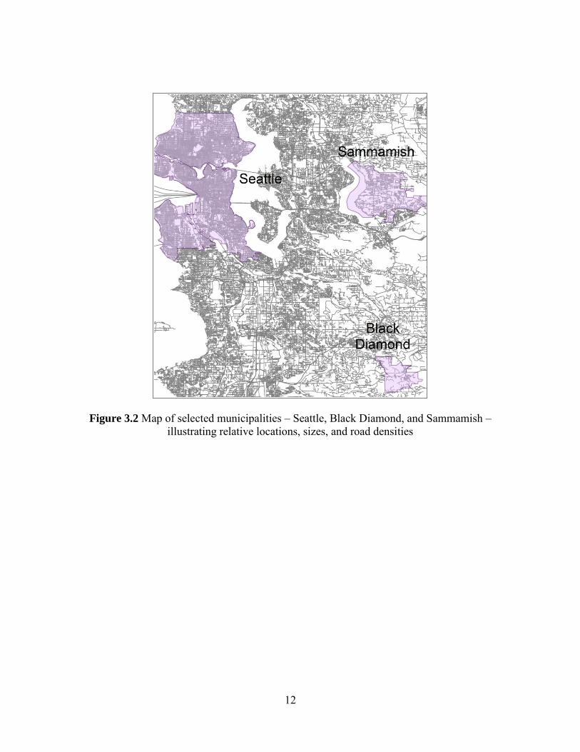
As illustrated in figure 3.1 Seattle has relatively high address density and moderate road density.
After eliminating outliers and places with fewer than 1000 residents, Black Diamond and Sammamish
were selected as two of the most contrasting locations, with low address and road densities. Their relative
locations, sizes, and road densities are illustrated in figure 3.2. Table 3.2 illustrates the descriptive
statistics for each municipality.
1414
Black Diamond
Sammamish
Seattle
12
Figure 3.2 Map of selected municipalities – Seattle, Black Diamond, and Sammamish – illustrating relative locations, sizes, and road densities
18

13
Table 3.2 Descriptive statistics for selected municipalities – Seattle, Black Diamond, and Sammamish
3.4 Depot Locations
Delivery services are generally clustered into two primary types – ones that rely on existing
brick-and-mortar retail locations for depots and those that use warehouses as depots. While other models
exist, this research compares these two main types: a brick-and-mortar storefront depot with a
warehouse-based model. This analysis considers replacing one roundtrip by an address to its nearest
grocery store with delivery from a local store-based delivery service or service from a regional
warehouse. Earlier work by the authors (Wygonik and Goodchild 2012) used one service area for
personal travel and delivery service, and this work is designed to develop a more realistic model of the
delivery service. For companies operating a delivery service out of a store-front, they are unlikely to
operate that company out of every store front. Rather, they would likely pick a small subset of available
options which would serve as depots for different quadrants of the city. This change reflects more realistic
catchment areas for retail stores versus a delivery depot.

14
Puget Sound Regional Council provided a shapefile with the locations of the major grocery stores
within King, Kitsap, and Snohomish counties. The service areas of the stores were calculated (using the
Service Area tool within ArcGIS Network Analyst) and addresses were assigned to their closest store’s
service area for the personal travel calculations. Cairns (1995) summarizes the results from six surveys to
describe the typical grocery shopping patterns in the United Kingdom. She cites a 1993 survey showing
nearly two-thirds of housewives grocery shop less than two miles from home and a survey by Telephone
Survey LTD, which indicated “62% of car shoppers use the nearest store to their home ‘of its type’ for
main food shopping” (Cairns 1995, pg. 412). Her summary also indicated the vast majority of households
with a car (99.6%) in the UK use a car for shopping, though in certain districts that percentage is
somewhat lower (Cairns 1995). Siikvavirta et al. (2002) indicate in Finland only 55%of households use a
car to grocery shop. Similarly detailed data are not available in the United States, where the National
Household Travel Survey (US DOT 2003) consolidates all shopping into one category. Analysis of the
2001 NHTS by Pucher and Renne (2003) indicates 91.5% of all shopping trips in the U.S. were made by
personal automobile. Market research by the Nielsen Company indicates value is the primary
consideration for 60% of U.S. shoppers when choosing a grocery store, followed by goods selection
(28%) and closest store (23%) (2007). While value is considered more important than proximity for more
Americans, the survey report did not indicate secondary and tertiary considerations. For this analysis,
assigning customers to their nearest store is reasonable, and provides a baseline for comparisons between
personal travel and delivery vehicles.
One in 5 stores throughout King County were selected to serve as local depots. This value
compares with the roughly 1 in 3 stores Tesco.com uses as local depots in the UK (Punakivi and
Tanskanen, 2002). As a result, a subset of five stores was selected to serve as depots for the store-based
delivery service in Seattle. These stores are distributed throughout Seattle and are illustrated in figure 3.3.
Black Diamond and Sammamish are each served by one local depot. In Black Diamond that depot is
outside the city limits. One existing warehouse location in Kent, Washington was selected to serve as the

15
depot location for the warehouse-based delivery service, as well as the warehouse serving the grocery
stores themselves (fig. 3.4).
Figure 3.3 Warehouse, depot, and store locations in Seattle

16
Figure 3.4 Warehouse, depot, and store locations for the three studied municipalities
3.5 Household Data
Geographic data regarding households and parcels were gathered from the Washington State
Geospatial Data Archive (WAGDA) and the Urban Ecology Lab at the University of Washington. To
maintain consistency with prior work, in Seattle only household location were selected. That effort
required joining the WAGDA King County parcels file (containing address data) to the Urban Ecology
Lab King County parcels file (containing the residential units data) to geocode the parcels with residential
units information, and selecting out the residential parcels. For Black Diamond and Sammamish, all
addresses were used as potential customers, reflecting that both households and businesses receive
delivery services.

17
As personal communication with local delivery providers indicate each truck can hold
approximately 35 households worth of orders, 35-household samples are used here. A total of 25 samples
for each municipality were gathered, as that ensured adequate statistical power while providing
reasonable computation time. For Seattle, 5 samples were gathered for each of the 5 local depot service
areas. For Black Diamond and Sammamish, 25 samples were gathered for the local depot service area.
These samples were used for all three travel types – household travel to their proximate store, delivery
service from their assigned store-based depot, and delivery service from the regional warehouse –
enabling direct comparison between each. The sampling was conducted randomly, with replacement,
from all available customers in the local depot service area. To evaluate the impacts of personal travel, the
sampled customers were then assigned to their closest store.

18

19
Chapter 4 Method
4.1 Scenarios
Three scenarios were considered in this evaluation:
1) The baseline scenario, Passenger Vehicles, represents a common form of travel for grocery
shopping. A large, combination truck stocks the grocery stores from the regional warehouse.
Individual customers use passenger vehicles to complete roundtrips from their addresses to
their closest grocery store and back.
2) The second scenario, Local Depot Delivery, provides delivery service from selected grocery
retail locations distributed throughout the region. In this scenario, the local depots are stocked
from the regional warehouse using large, combination trucks. Then smaller box trucks
complete delivery via a milk-run starting and ending at the select stores and stopping at the
sampled customers along the way.
3) The third scenario, Regional Warehouse Delivery, provides delivery service directly from the
regional warehouse using small, box trucks. The routes start and end at the regional
warehouse and stop at the sampled customers along the way.
These scenarios are illustrated in figure 4.1.

20
Pass
enge
r Veh
icle
s
Loca
l Dep
ot D
eliv
ery
Reg
iona
l War
ehou
se D
eliv
ery
Figure 4.1 System bounds and vehicle types for three scenarios
Regional Warehouse
Home
Home
Home
Home
Home
Home
Home
Home
Home
Home
Home
Home
HomeHome
HomeHome
GroceryStore
GroceryStore
GroceryStore
GroceryStore
Combination Truck
Single-unit Truck
Passenger Car
Regional Warehouse
Home
Home
Home
Home
Home
Home
Home
Home
Home
Home
Home
Home
HomeHome
HomeHome
GroceryStore
GroceryStore
GroceryStore
GroceryStore
GroceryStore
GroceryStore
GroceryStore
GroceryStore
Regional Warehouse
Home
Home
Home
Home
Home
Home
Home
Home
Home
Home
Home
Home
HomeHome
HomeHome

21
4.2 Vehicle travel
To estimate the distances traveled and the associated emissions, routing tools within ArcGIS
Network Analyst were used.
To complete the routing estimates, the Network Analyst Closest Facility tool was used to
calculate the distance traveled to each grocery store for each household in the sample for the Passenger
Vehicle scenario. The StreetMap network was loaded for use with Network Analyst. Output from
Network Analyst includes the one-way distance traveled for each residential unit and the one-way
emissions associated with each residential unit’s grocery store trip when the trip is optimized for shortest
time. These outputs were doubled, to reflect round trip distances and emissions. Using round trips for the
Passenger Vehicle scenario represents a simplification, as some grocery shopping does occur within
chained trips. However, the available data do indicate most grocery shopping occurs via passenger vehicle
making exclusive trips (as discussed above and outlined in Wygonik and Goodchild 2012). Not all trips
would be replaced by this type of service, but it is a reasonable estimation of the impact of replacing main
household stocking trips.
To complete the routing estimates, the Network Analyst Routing tool was used to calculate the
distance traveled by a delivery vehicle starting and ending at the depots and serving a sample of 35
households. The StreetMap network was loaded for use with Network Analyst. Network Analyst was run
to identify the fastest path to serve the given households. The analysis reordered the stops to identify the
fastest route, but kept the first and last stops (the depot) constant. Output from Network Analyst includes
the distance traveled for each delivery vehicle and emissions associated with each tour, with the route
optimized for shortest time.
Vehicle travel to stock the grocery stores from the regional warehouse was also included to
maintain a constant system boundary for all scenarios. For the personal travel, 10 tractor trailers were

22
required to stock the 49 grocery store locations proximate to Seattle. The Network Analyst Routing tool
was used to calculate the distance traveled and emissions for 10 tractor trailers leaving the regional
warehouse and each serving 5 stores (one served 4). The results were then divided by 10 to represent the
average values for one truck. For Black Diamond, the 5 stores closest to the one serving Black Diamond
were selected and served by a tractor trailer. For Sammamish, the 10 closest stores were selected and
served by two tractor trailers for stocking runs.
For the scenario involving the local, store-based depots, the Network Analyst Routing
tool was used to calculate the distance traveled and emissions for one tractor trailer serving the 5
store-based depots in Seattle and the closest 5 depots to Black Diamond and Sammamish. Figure
4.1 above illustrates the 3 scenarios.
4.3 Assumptions
A number of assumptions were required within the modeling system. First, all optimizations used
hard time windows, guaranteeing that promised delivery times would be met. The problem is also
simplified to an urban delivery system, disregarding pickup. The model does not consider real-time
routing changes. It is a planning tool and is not intended to provide dynamic routing information. In
addition, this model currently assumes uncongested conditions.
4.4 Regression modeling
The regression modeling was conducted using the R statistical package. This evaluation relied on
the same set of sampled addresses used above, but in this case each address represented a data point with
information about VMT and CO2, PM10, and NOx emissions associated with each of the three goods
movement scenarios along with descriptive data about an addresses associated land use environment
(address density, distance to the warehouse, etc.). As a result, the regression estimates were conducted on
the entire set of sampled addresses, with a sample size of 2625 (25 addresses, sampled 35 times, in 3
municipalities). Because of the sampling with replacement initially conducted, a small subset of the

23
sampled addresses may be included more than once. This value is expected to be small enough to not
affect the outcome.
To estimate the models, a modified forward selection was conducted on the likely variables. Each
variable was tested for fit, and the variable with the highest explanatory power that was also significant
was added to the model. This new model was tested with each of the remaining variables. If any of those
remaining variables were significant, the model with the new highest predictive power was selected as the
current active model. This process was repeated until either all variables were added to the model or new
variables were not significant.
Two difference sets of models were developed. The first set of models represented the Best Fit
models, and these models included all variables that tested significant within the model estimation. The
second set of models represent the Parsimonious models. These models include only the variables that
meaningfully improve the explanatory power.
Models for each dependent variable (VMT, CO2, NOx, and PM10) were developed for each
goods movement structure, for a total of 12 models in each of the two sets.
The variables selected in these models were then tested for influence in the comparative
relationships between goods movement strategies. The two sets of models were again developed for each
dependent variable, but this time a subset of models was created representing the differences between
passenger vehicle travel and local depot delivery, between passenger vehicle travel and warehouse-based
delivery, and between local depot delivery and warehouse-based delivery. Again, a total of 24 models
were estimated.
Based on the literature, the following variables were tested for each goods movement strategy.
For Passenger Travel, the tested variables include:
Address Density : the number of addresses in the store service area divided by the store
service area size (units = 1/square mile)
Store Service Area Size : the store service area size (square mile)

24
Distance from the Warehouse to the Store : the on-road travelled distance between the
warehouse and the assigned store (miles), calculated using Google maps and the location
addresses
Store Service Area Road Density : the linear feet of road in a store service area divided by the
store service area size (feet/square feet)
Store Service Area Junction Density : the number of junctions in a store service area divided
by the store service area size (1/square feet)
A similar set of variables was tested for the Local Depot Delivery models, but these variables
were standardized by the depot service area instead of the store service area.
Customer Density : the number of customers in the depot service area divided by the depot
service area size (units = 1/square mile)
Depot Service Area Size : the store service area size (square mile)
Distance from the Warehouse to the Depot : the on-road travelled distance between the
warehouse and the assigned depot (miles) , calculated using Google maps and the location
addresses
Depot Service Area Road Density : the linear feet of road in a depot service area divided by
the depot service area size (feet/square feet)
Depot Service Area Junction Density : the number of junctions in a depot service area divided
by the depot service area size (1/square feet)
Distance from the Depot to the Depot Service Area Centroid : the on-road travelled distance
between the depot and the geographic centroid of the depot service area (miles), calculated
using Network Analyst tools in ArcGIS
The variables tested for Warehouse Delivery were the same as those tested for Local Depot
delivery, except a different measure for travel distance from the warehouse was used.
Customer Density
Depot Service Area Size

25
Depot Service Area Road Density
Depot Service Area Junction Density
Distance from the Warehouse to the Depot Service Area Centroid : the on-road travelled
distance between the warehouse and the geographic centroid of the depot service area (miles)
, calculated using Network Analyst tools in ArcGIS
Additional variables were developed for the goods movement strategy comparisons. These were
ratios between like variables. For example, the passenger travel models were evaluated for the road
density in the store service area, while the delivery models were evaluated for the road density in the
depot service area. For the comparison models, an extra variable representing the ratio of store service
area road density to depot service area road density was included.
Descriptive statistics for all evaluated variables are included in table 4.1. The correlation
plot between these variables is illustrated in fig 4.2. As is shown, the different measures of
distance among the warehouse, stores, depots, and centroids were highly correlated. The various
measures of road and junction density were highly correlated.
Table 4.1 Descriptive statistics for evaluated independent variables
Minimum
Value Mean
Maximum
Value
Standard
Deviation Units
Store Service Area Road Density 6.0 15.6 37.5 7.81 miles/square mile
Distance: Warehouse to Store 10.8 19.2 29.4 6.31 miles
Address Density 20.5 1009.1 2886.5 760.56 1/square miles
Store Service Area Junction Density 56.6 179.9 637.0 116.88 1/square miles
Store Service Area Size 0.5 6.6 20.6 3.95 square miles
Customer Density 1.6 2.9 4.9 1.43 1/square miles
Depot Service Area Road Density 9.8 16.3 31.9 8.64 miles/square mile
Distance: Warehouse to Depot 12.5 19.1 25.7 5.80 miles
Depot Service Area Junction Density 70.3 204.8 530.0 146.49 1/square miles
Distance: Depot to Centroid 0.2 2.1 4.2 1.51 miles
Distance: Warehouse to Centroid 12.8 20.0 27.0 5.89 miles
Store:Depot Service Area Road Density 0.60 0.98 1.31 0.17
Distance - Warehouse to Store: Warehouse to Centroid 0.72 0.96 1.25 0.09
Distance - Warehouse to Centroid: Warehouse to Depot 0.93 1.05 1.14 0.08
Distance - Warehouse to Store: Warehouse to Depot 0.67 1.00 1.19 0.07

26
Figure 4.2 Correlations between evaluated independent variables

27
Chapter 5 Results
5.1 Evaluation of goods movement schemes by municipality
Figure 5.1 and figure 5.2 illustrate the service areas for the grocery stores and local depots. The
35-household samples were drawn from the households within each depot service area. One of the
stocking routes used to supply the stores or local depots is shown in figure 5.1. One of the household
samples and the associated routes for passenger travel and for local-depot-based delivery are shown in
figure 5.2.
Warehouse to Stores
(Combination Short Haul Truck)
Warehouse to Local Depots
(Combination Short Haul Truck)
Figure 5.1 Illustrations of example stock routes

28
Passenger Vehicles
(Passenger Cars)
Delivery Vehicle
(Single-Unit Short Haul Truck)
Figure 5.2 Illustrations of example final travel to homes
Looking at the results from the three different delivery structures (fig. 5.3), the relative
contributions of the different legs of the supply chain become apparent. Personal travel requires the
largest number of vehicle miles traveled but generates moderate levels of pollutants. Any use of a
combination short haul truck within a supply chain involves significant emissions production, while the
passenger cars contribute very small amounts of the studied emissions and practically no PM10.
Combination short haul trucks have particularly high rates of NOx emissions, relatively. In Black
Diamond, where the regional warehouse delivery system generates only slightly higher levels of VMT

29
than the local depot delivery system but fewer emissions of NOx and PM10, the relative impact of the
combination short haul trucks is apparent.
Seat
tle
0
1
2
3
4
5
6
7
8
Pas
sen
ger
Ve
hic
le
Loca
l De
live
ry
Re
gio
nal
De
live
ry
Pas
sen
ger
Ve
hic
le
Loca
l De
live
ry
Re
gio
nal
De
live
ry
Pas
sen
ger
Ve
hic
le
Loca
l De
live
ry
Re
gio
nal
De
live
ry
Pas
sen
ger
Ve
hic
le
Loca
l De
live
ry
Re
gio
nal
De
live
ry
Pas
sen
ger
Ve
hic
le
Loca
l De
live
ry
Re
gio
nal
De
live
ry
VMT CO2 (kg) NOx (g) PM10 (dg) Travel time (min)
Combination Short Haul Single-unit Short Haul Passenger Cars

30
Bla
ck D
iam
ond
Sam
mam
ish
Figure 5.3 Results for each delivery structure, by vehicle type
0
2
4
6
8
10
12
14
Pas
sen
ger
Ve
hic
le
Loca
l De
live
ry
Re
gio
nal
De
live
ry
Pas
sen
ger
Ve
hic
le
Loca
l De
live
ry
Re
gio
nal
De
live
ry
Pas
sen
ger
Ve
hic
le
Loca
l De
live
ry
Re
gio
nal
De
live
ry
Pas
sen
ger
Ve
hic
le
Loca
l De
live
ry
Re
gio
nal
De
live
ry
Pas
sen
ger
Ve
hic
le
Loca
l De
live
ry
Re
gio
nal
De
live
ry
VMT CO2 (kg) NOx (g) PM10 (dg) Travel time (min)
Combination Short Haul Single-unit Short Haul Passenger Cars

31
Table 5.1 displays the data that supports figure 5.3. It includes averaged data about each leg of the
supply chain for each scenario: the trip from warehouse to store or depot and the trip from the store or
depot to the addresses or the trip directly from the warehouse to the addresses.
Local Depot Delivery service – where a single-unit short haul truck delivers to homes from a
local depot stocked by a combination short haul truck – requires the lowest amount of VMT. The
efficiency of delivery is highlighted by comparing the amount of VMT generated by passenger cars
compared to the corresponding final-leg delivery vehicle. Even when the delivery vehicle is serving
homes from a regional warehouse, it still requires fewer VMT than if individual homes travel directly to
their closest grocery store.
The results in table 5.1 also highlight the benefit of delivering to stops that are clustered together.
While the combination trucks all serve 5 stores or depots, the stores are clustered together in the routes.
The depots are spread throughout the city or region and require more travel to serve from the warehouse.
Further, the personal vehicles require twice as much travel to get from the homes to the stores as the
delivery vehicle requires to serve those homes from a local depot even though the personal travel goes to
the closest store and the local depot is serving an entire quadrant of the city.
By leveraging the efficiency of a delivery structure, local depot delivery directly has the lowest
VMT any of the cases. A goods movement system relying on passenger vehicles for the last mile has the
highest levels of VMT and the highest levels of CO2 for two of the municipalities. It does, however,
produce the lowest levels of the studied criteria pollutants (NOx and PM10) for the three municipalities.
The goods movement system producing the lowest levels of CO2 varies by municipality, with each of the
three studied locations relying on a different goods movement structure to minimize carbon dioxide
generation. The two delivery systems produce the highest criteria pollutants, but the least efficient system
varies by municipality.

32
Table 5.1 Vehicle miles traveled, emissions, and travel time by supply chain leg and design
Seat
tle
Bla
ck D
iam
ond
Sam
mam
ish
Table 5.2 summarizes the goods movement system that produces the highest and lowest levels of
VMT, CO2, Nox, PM10, and Travel Time for each municipality.
VMT CO2 (kg) Nox (g) PM10 (dg)
Travel time
(min)
To stores 0.3 0.5 2.2 0.8 0.4
To addresses 1.8 0.6 0.6 0.2 3.5
Total 2.1 1.1 2.7 1.0 3.8
To depots 0.3 0.7 2.8 1.2 0.5
To addresses 0.8 1.1 3.7 1.6 1.6
Total 1.1 1.7 6.5 2.8 2.1
To addresses 1.7 1.8 6.9 3.1 2.8
Last Mile Personal Travel
Local Depot Truck Delivery
Regional Truck Delivery
VMT CO2 (kg) Nox (g) PM10 (dg)
Travel
time (min)
To 5 stores 0.2 0.3 1.3 0.6 0.3
To addresses 8.3 2.7 2.5 0.7 13.5
Total 8.4 3.0 3.8 1.3 13.8
To 5 depots 0.5 0.9 3.8 1.6 0.7
To addresses 0.9 1.1 4.2 1.8 1.9
Total 1.4 2.0 8.0 3.4 2.6
To addresses 1.5 1.7 6.8 2.9 2.9Regional Truck Delivery
Last Mile Personal Travel
Local Depot Truck Delivery
VMT CO2 (kg) Nox (g) PM10 (dg)
Travel
time (min)
To 10 stores 0.3 0.6 2.7 1.0 0.5
To addresses 8.3 2.7 2.5 0.7 13.5
Total 8.6 3.3 5.2 1.7 14.0
To 5 depots 0.5 0.9 3.8 1.6 0.7
To addresses 1.2 1.5 5.8 2.5 2.6
Total 1.6 2.4 9.6 4.1 3.3
To addresses 2.5 2.6 10.3 4.6 4.3Regional Truck Delivery
Local Depot Truck Delivery
Last Mile Personal Travel

33
Table 5.2 Summary of delivery structure impacts
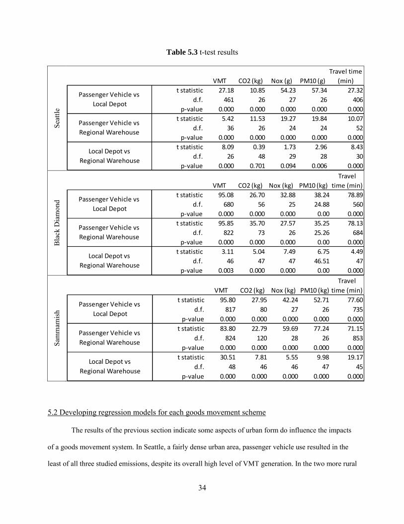
The results were also evaluated for significance using the two-tailed t-test. All comparisons were
significantly different with p-values (p≤0.001), except for the difference in pollution generation between
the two delivery systems in Seattle and the difference in VMT for the two delivery systems in Black
Diamond. In Seattle, no significant difference between the two delivery systems was observed in the
generation of CO2. The difference in NOx generation in Seattle between the two delivery systems was
significant only at the p≤0.1 level, and the difference in PM10 generation was significant at the p≤0.01
level. The difference in VMT between the two delivery systems in Black Diamond was significant at the
p≤0.005 level.
Detailed results of the t-tests are included in table 5.3 and illustrate that variations across samples
are small compared to the variation between scenarios.
34
Table 5.3 t-test results
Seat
tle
Bla
ck D
iam
ond
Sam
mam
ish
5.2 Developing regression models for each goods movement scheme
The results of the previous section indicate some aspects of urban form do influence the impacts
of a goods movement system. In Seattle, a fairly dense urban area, passenger vehicle use resulted in the
least of all three studied emissions, despite its overall high level of VMT generation. In the two more rural
VMT CO2 (kg) Nox (g) PM10 (g)
Travel time
(min)
t statistic 27.18 10.85 54.23 57.34 27.32
d.f. 461 26 27 26 406
p-value 0.000 0.000 0.000 0.000 0.000
t statistic 5.42 11.53 19.27 19.84 10.07
d.f. 36 26 24 24 52
p-value 0.000 0.000 0.000 0.000 0.000
t statistic 8.09 0.39 1.73 2.96 8.43
d.f. 26 48 29 28 30
p-value 0.000 0.701 0.094 0.006 0.000
Local Depot vs
Regional Warehouse
Passenger Vehicle vs
Regional Warehouse
Passenger Vehicle vs
Local Depot
VMT CO2 (kg) Nox (kg) PM10 (kg)
Travel
time (min)
t statistic 95.08 26.70 32.88 38.24 78.89
d.f. 680 56 25 24.88 560
p-value 0.000 0.000 0.000 0.00 0.000
t statistic 95.85 35.70 27.57 35.25 78.13
d.f. 822 73 26 25.26 684
p-value 0.000 0.000 0.000 0.00 0.000
t statistic 3.11 5.04 7.49 6.75 4.49
d.f. 46 47 47 46.51 47
p-value 0.003 0.000 0.000 0.00 0.000
Local Depot vs
Regional Warehouse
Passenger Vehicle vs
Local Depot
Passenger Vehicle vs
Regional Warehouse
VMT CO2 (kg) Nox (kg) PM10 (kg)
Travel
time (min)
t statistic 95.80 27.95 42.24 52.71 77.60
d.f. 817 80 27 26 735
p-value 0.000 0.000 0.000 0.000 0.000
t statistic 83.80 22.79 59.69 77.24 71.15
d.f. 824 120 28 26 853
p-value 0.000 0.000 0.000 0.000 0.000
t statistic 30.51 7.81 5.55 9.98 19.17
d.f. 48 46 46 47 45
p-value 0.000 0.000 0.000 0.000 0.000
Passenger Vehicle vs
Local Depot
Passenger Vehicle vs
Regional Warehouse
Local Depot vs
Regional Warehouse

35
municipalities – Black Diamond and Sammamish – delivery options were able to reduce CO2 emissions
even if they could not reduce criteria pollutants. However, there are a number of differences among these
places. They vary in terms of their customer density, network density, number of stores and depots, and
their distance to the regional warehouse. To shed some light into the factors that influence VMT and
emissions generation, regression models were developed for each of the three goods movement methods.
As discussed in the Methods section, a modified forward selection was conducted to develop Best Fit and
Parsimonious models. For this analysis, all of the delivery addresses for all three municipalities were
combined into one data set to enable testing of the variables discussed above, resulting in a sample size of
2625 addresses. Table 5.4 illustrates the resulting models for each of 4 dependent variables for each of
the three goods movement strategies.
Table 5.4 Best fit models for each goods movement strategy
Pass
enge
r Veh
icle
Loca
l Dep
ot D
eliv
ery
r^2 Intercept
Store Service
Area Road
Density
Distance:
Warehouse to
Store
Address
Density
Store Service
Area Junction
Density
Store Service
Area Size
VMT 0.686 10.990 -0.286 0.045 -0.001
Co2 0.659 3.598 -0.088 0.031 -0.0003
NOx 0.698 2.879 -0.034 0.111 -0.0003 -0.001 0.013
PM10 0.600 0.102 -0.001 0.003 -0.00001 -0.00003 0.0004
r^2 Intercept
Depot Service
Area Road
Density
Distance:
Warehouse to
Depot
Depot Service
Area Junction
Density
Distance: Depot
to Centroid
VMT 0.822 1.190 -0.028 0.024 0.001 0.032
Co2 0.647 1.833 -0.035 0.029 0.001 0.020
NOx 0.873 7.006 -0.181 0.135 0.004 0.229
PM10 0.871 0.294 -0.008 0.006 0.0002 0.010

36
Reg
iona
l War
ehou
se
Del
iver
y
As seen in table 5.4, a relatively small number of variables influences each model. Further, the
variables that influence the models for each delivery structure are consistent, with the same variables
appearing in all four models across each of the local depot and regional warehouse delivery models. For
the passenger vehicle structure, the models for VMT and CO2 result in the same set of selected variables,
as do the models for NOx and PM10. The models shown here all explain at least 60 percent of the
variation observed, with as much as 95 percent of the variation observed for regional warehouse delivery
explained. All of the models rely on a form of road density and distance from the warehouse to some part
of the service area. Junction density and customer or address density appear in a majority of the models.
Lastly, the coefficients have consistent signs across most of the models. Road density always has
a negative influence (increased road density results in lower VMT, CO2, NOx, and PM10). An increased
distance between the warehouse and service area always results in higher values for the dependent
variables. Increased customer density results in lower VMT but higher CO2, NOx, and PM10 for the
regional warehouse delivery. In contrast, increased address density for passenger vehicle travel results in
lower VMT and lower CO2, NOX, and PM10 emissions. The junction density variables have consistent
signs for the delivery models (increased junction density increases the VMT, CO2, NOx, and PM10), but
those signs are opposite the signs for junction density in the passenger travel models for NOx and PM10.
While these models are explanatory, they have two primary limitations. First, simpler models
explain much of the variation observed in the Best Fit models. Second, some of the independent variables
r^2 InterceptCustomer
Density
Depot Service
Area Road
Density
Depot Service
Area Junction
Density
Distance:
Warehouse to
Centroid
VMT 0.969 0.567 -0.008 -0.018 0.001 0.077
Co2 0.945 0.930 0.022 -0.028 0.001 0.067
NOx 0.948 3.602 0.075 -0.112 0.003 0.266
PM10 0.956 0.149 0.002 -0.005 0.0001 0.013

37
included in the Best Fit models covary. For example, the variables for junction density and road density
are highly correlated. For these reasons, Parsimonious Models were developed. These models are seen in
table 5.5.
Table 5.5 Parsimonious models for each goods movement strategy
Pass
enge
r Veh
icle
Loca
l Dep
ot D
eliv
ery
Reg
iona
l War
ehou
se
Del
iver
y
As seen in table 5.5, these models can be reduced to one or two variables: some measure of road
density and some measure reflecting the distance from the warehouse to the service area. The r^2 values
for the Best Fit models are no more than 0.018 better, and as little as 0.002 improvement is seen. In all of
the Parsimonious Models, road density negatively influences the dependent variables, and the distance
from the warehouse to the service area has a positive influence.
r^2 Intercept
Store Service
Area Road
Density
Distance:
Warehouse to
Store
VMT 0.677 12.127 -0.369
Co2 0.641 4.300 -0.114
NOx 0.692 3.507 -0.081 0.094
PM10 0.596 0.118 -0.002 0.003
r^2 Intercept
Depot Service
Area Road
Density
Distance:
Warehouse to
Depot
VMT 0.818 1.343 -0.021 0.020
Co2 0.643 1.876 -0.024 0.028
NOx 0.865 8.054 -0.129 0.109
PM10 0.864 0.034 -0.006 0.005
r^2 Intercept
Depot Service
Area Road
Density
Distance:
Warehouse to
Centroid
VMT 0.967 0.424 -0.009 0.081
Co2 0.942 0.980 -0.016 0.066
NOx 0.945 3.700 -0.062 0.266
PM10 0.953 0.149 -0.003 0.013

38
5.3 Developing regression models for goods movement scheme comparisons
The variables identified in the previous section, which influence the studied impacts of the three
goods movement strategies, were used to focus evaluations of the comparative impacts of the strategies.
Models were developed for each comparison (passenger vehicle travel vs. local depot delivery, passenger
vehicle travel vs. regional warehouse delivery, and regional warehouse delivery vs. local depot delivery)
for each of the studied impacts. The variables that appear in the Parsimonious models for the two goods
movement strategies under consideration were included in the regression analysis. For example, when
evaluating the variables that influence the relative impacts of passenger vehicle travel versus local depot
delivery, Store Service Area Road Density, Depot Service Area Road Density, Distance from Warehouse
to Store, and Distance from Warehouse to Depot were included. Further, ratios comparing Store Service
Area Road Density to Depot Service Area Road Density and the two distances were also developed and
included. This model therefore had six potential variables included. The results for the Best Fit models are
shown in table 5.6.
Table 5.6 Best fit models for goods movement strategy comparisons
Pass
enge
r Veh
icle
s vs.
Loca
l Dep
ot D
eliv
ery
Pass
enge
r Veh
icle
s vs.
War
ehou
se D
eliv
ery
r^2 Intercept
Store Service
Area Road
Density
Distance:
Warehouse to
Store
Depot Service
Area Road
Density
Distance:
Warehouse to
Depot
Store:Depot
Service Area
Road Density
VMT 0.699 9.084 -0.187 -0.017 -0.155 1.706
Co2 0.556 1.455 -0.066 -0.023 -0.009 0.620
NOx 0.238 -5.050 -0.033 0.077 0.331
PM10 0.546 -0.230 0.004 -0.001
r^2 Intercept
Store Service
Area Road
Density
Distance:
Warehouse to
Store
Depot Service
Area Road
Density
Distance:
Warehouse to
Centroid
Store:Depot
Service Area
Road Density
Distance
Warehouse
to Store:
Warehouse
to Centroid
VMT 0.708 9.548 -0.198 -0.072 -0.151 1.895
Co2 0.609 3.723 -0.057 0.057 -0.033 -0.098 0.517 -1.545
NOx 0.653 -1.174 -0.067 0.055 -0.162 0.615
PM10 0.838 -0.053 -0.002 0.003 -0.010 0.021

39
Reg
iona
l War
ehou
se
vs. L
ocal
Dep
ot
Del
iver
y
Most of the Best Fit models were able to explain more than half the variation in the comparisons.
However, once again, the Best Fit models included variables that covary and did not provide significantly
more explanatory power than simpler models. Table 5.7 illustrates the resulting Parsimonious models.
Table 5.7 Parsimonious models for goods movement strategy comparisons
Pass
enge
r Veh
icle
s vs.
Loca
l Dep
ot D
eliv
ery
Pass
enge
r Veh
icle
s vs.
War
ehou
se D
eliv
ery
r^2 Intercept
Depot Service
Area Road
Density
Distance:
Warehouse to
Depot
Distance:
Warehouse to
Centroid
Distance
Warehouse to
Centroid:
Warehouse to
Depot
VMT 0.979 -0.710 0.003 0.052 0.010
Co2 0.644 -0.813 0.005 0.038
NOx 0.953 -7.938 0.009 0.581 -0.403 4.469
PM10 0.966 -0.265 0.001 0.020 -0.011 0.106
r^2 Intercept
Depot Service
Area Road
Density
Distance:
Warehouse to
Depot
VMT 0.691 10.252 -0.322
Co2 0.544 1.840 -0.082
NOx 0.235 -4.754 0.047
PM10 0.546 -0.230 0.004 -0.001
r^2 Intercept
Distance:
Warehouse to
Store
Depot Service
Area Road
Density
Distance:
Warehouse to
Centroid
VMT 0.701 11.086 -0.065 -0.328
Co2 0.599 2.620 -0.040 -0.085
NOx 0.644 -0.789 -0.158
PM10 0.835 -0.037 0.001 -0.010

40
Reg
iona
l War
ehou
se v
s. Lo
cal D
epot
Del
iver
y
As with the individual models, one or two variables was able to explain much of the variation
observed. Variable selection for the parsimonious models relied only on direct measures of distance and
road density, and none of the ratios were selected for these models. Further, once again the r^2 values are
not substantially larger with the Best Fit models than the parsimonious models. Differences as little as
0.001 and not larger than 0.012 are observed between the r^2 values.
Using this information along with the differences observed in the estimated impacts for each
municipality allows us to evaluate the tipping point for CO2 reduction when replacing Passenger Vehicle
travel. Solving for 0 with equation 5.1, indicates that when the road density in the depot service area is at
least 22.43 miles/square mile, passenger travel will result in lower CO2 emissions than local depot
delivery. Black Diamond’s 78 linear miles of road represent 10 linear miles of road for every square mile,
and Sammamish’s 215 linear miles of road represent about 9.7 linear miles of road for every square mile.
In contrast, Seattle’s over 2000 linear miles of road represent more than 24 linear miles of road for every
square mile of land – just above the threshold. The relationships between the studied municipalities and
the identified threshold is illustrated in figure 5.4. The difference in CO2 between passenger travel and
local depot delivery is
CO2 passenger travel-local depot delivery = 1.840-0.082 * δ (5.1)
where δ : Depot Service Area Road Density.
r^2 Intercept
Depot Service
Area Road
Density
Distance:
Warehouse to
Depot
Distance:
Warehouse to
Centroid
VMT 0.978 -0.662 0.062
Co2 0.644 -0.813 0.005 0.038
NOx 0.949 -3.565 0.030 0.159
PM10 0.965 -0.165 0.001 0.008

41
Figure 5.4 Studied municipalities and other King County, Washington municipalities
Because the parallel equation comparing passenger vehicle travel and warehouse delivery
relies on two variables (equation 5.2) the tipping point cannot be solved. However, the graph
below illustrates the sensitivity analysis for the two variables. Any point below the line is a
scenario in which Warehouse-based Delivery is estimated to generate lower CO2 emissions than
Passenger vehicle travel (see fig. 5.5). Figure 5.6 illustrates where the municipalities in King
County, Washington – including the ones studied here – fall relative to that line. The difference
in CO2 between passenger travel and warehouse-based delivery is
CO2 passenger travel-warehouse-based delivery = 2.620-0.04*L-0.085 * δ (5.2)
Where L : Distance from Warehouse to Store δ : Depot Service Area Road Density.
3737
Black Diamond
Sammamish
Seattle

42
Figure 5.5 Sensitivity analysis threshold comparing influences on CO2 emissions between passenger vehicles and warehouse delivery goods movement schemes
Figure 5.6 Studied Municipalities and Other King County, Washington Municipalities Compared to Distance to Warehouse and Road Density Thresholds between Passenger Travel
and Regional Delivery for CO2 Emissions
0
5
10
15
20
25
30
35
0 15 30 45 60 75
Dep
ot
Serv
ice A
rea R
oad
Den
sit
y
(ft/
ft2)
Distance from Warehouse to Store (mi)
4040
Black DiamondSammamish
Seattle

43
Chapter 6 Discussion
These results show notable sensitivity to the structure of the depot, the depot location, routes
traveled, and business model. Earlier work by Wygonik and Goodchild (2012) found delivery services
reduced VMT and CO2 emissions when used in lieu of passenger vehicle travel. These results
conditionally support those findings. Understanding operational details and including them in modeling
efforts is necessary to evaluate the efficacy of these services. On-going work should pursue the influence
of customer density thresholds, depot density, regional warehouse location sensitivity, and engine
technology. Delivery service is one method of addressing some of the externalities from transportation.
Further research will inform how to best leverage this transportation strategy. Shopping travel represents
14.5 percent of household vehicle miles travelled. (Hu and Reuscher 2004) Finding methods to reduce
VMT associated with shopping has significant potential to address total VMT and resulting emissions.
This analysis relied on data provided by a local supplier, in which 35-households are served from
a regional warehouse using one single-unit truck within the necessary time constraints. Different regional
land use patterns with higher levels of sprawl might require significantly more travel from the regional
warehouse to the urban center and restrict the number of households that can be served by each truck.
Alternatively, lower customer demand may alter the usage levels of the vehicles or higher customer
demand may enable more tightly clustered customers. While this analysis did not show particular
sensitivity to customer density, there is mathematical support for its influence. As such, testing the
assumptions in this work with different customer sample sizes and different truck occupancy levels is
suggested.
Distance to the warehouse was a significant variable in the models developed. However, the
variation in distance was limited. In rural places that are not as proximate to a major urban center, these
distances would be expected to be considerably longer. Further evaluation of the sensitivity of the models
to this variable is suggested.
In structuring this work, the author had expected to find a relationship between an aspect of the
store service area to an aspect of the delivery service area to explain the relative efficiency of the goods

44
movement strategies. This did not occur. Further, the author had anticipated customer density to be an
important variables. This also did not occur. In practice, only direct measures – not comparative ones –
informed the relative performance of the goods movement strategies. In addition, which density was
important, it was the road density, not the customer density that influenced the results. Exploring other
measures of transportation density and connectivity are therefore suggested.
A key aspect of this analysis is the assumed location of the local depots and the warehouse.
Given the importance of distance and road density, the results may be highly sensitive to the locations
chosen. Extensive random sampling of the households was conducted, but the depots were not similarly
varied. The author suggests an evaluation in which the number and location of local depots are varied, in
addition to the above suggestion to pursue a wider range of warehouse distances. Another aspect that may
be highly influential are the assumptions made in this analysis regarding the number of depots and stores
served by the stocking routes. As the relative contributions of the combination trucks are large, the results
could be sensitive to variations in these assumptions. In addition, the efficiency of these stocking routes
may vary with urban form – more distant and less dense areas may require less efficient stocking routes
because of the additional time required to serve those locations.
Finally, this analysis relied on business-as-usual transportation methods: diesel-engine tractor
trailers serving longer routes and bigger customers with single-unit diesel engine trucks or gasoline-
engine passenger vehicles serving customers. Transportation methods that rely on lower emission
technology (such as hybrid, electric, compressed natural gas or human-powered vehicles) or that involve
more efficient operations (trip-training for passenger vehicles) will change the impacts observed.
6.1 Limitations
This work provided useful insight regarding the relationship between land use and VMT,
and CO2, PM10, and NOx emissions. However, a number of limitations remain.

45
This work relied on data from King County, Washington. While the selected
municipalities reflected the range of densities observed in that county, it is not reflective of the
entire range of densities observed across the United States or in other countries.
The work also assumed a roundtrip was conducted between addresses and stores and that
roundtrip was replaced by a delivery service. While carpooling or using transit service to replace
a commute trip would be purely substitutional, the same relationship is not guaranteed with
shopping behavior. Personal shopping trips that are replaced by delivery service may be
backfilled with other trips, including other shopping trips. Further, a replacement may occur
between final purchase in store with an online purchase, but recent data indicates customers will
still shop in the store to gather data before making their purchase, so-called showrooming.
Lastly, while the evidence indicates most shopping transportation does occur with personal
vehicles and does involve roundtrips, some shopping does occur using walking, biking or transit
and some shopping is part of chained trips. In addition, this analysis assumed customers would
travel to the closest store. While the available data indicates this assumption is mostly true
(recall, customers were reported to shop at the closest store of its type), it is not strictly true and
has the effect of underestimating the impacts of the personal travel scenario. Some minor error is
introduced in that addresses but not individual units were sampled. Since zoning laws tend to
focus multifamily homes and multiple-occupant commercial space toward central business
districts and arterials, this sampling error has the potential to bias the results in the other
direction – overestimating the impacts from personal travel. These units are, however, the most
likely to take advantage of alternative modes to conduct shopping activities due to their
proximity.

46
Another limitation to generalizing these results, reflects the number and location of the
warehouses and depots. The results point to the influence of the distance to the warehouse on the
measures. Because of the land use patterns and physical constraints in King County, Washington
(due to bodies of water, mountains, and existing urban areas), the range of distances to the
warehouse was relatively small. Less geographically-constrained regions of the country may
have much longer distances to warehouses.
While some reductions in CO2 emissions were estimated through the use of delivery
service, this model is not able to include secondary benefits to CO2 emissions from congestion
reduction. This secondary effect will have the largest impact in urban areas which are already
significantly impacted by high levels of congestion. The more dense areas are the places where
reductions in CO2 emissions are not observed directly by replacing personal travel with delivery
service. While rural areas would be less impacted by secondary effects of congestion reduction,
the significant reductions seen in CO2 generation when personal travel is replaced by delivery
service could be eliminated if some of the personal travel trips are not eliminated but are
replaced by other travel.
Finally, this analysis assumed trucks would utilize existing diesel engine technology.
Diesel engines generate high levels of the evaluated pollutants and will limit the potential
advantage of VMT reductions. Leveraging other types of engine technology may allow delivery
services to positively affect all evaluated measures and eliminate the observed trade-offs.

47
Chapter 7 Conclusions and Recommendations
This work supports earlier findings that VMT can be reduced by delivery schemes. Earlier efforts
found VMT reduction between passenger travel and delivery vehicles to range from 50 to 95 percent
(Cairns 1997, 1998, 2005; Punakivi and Saranen, 2001; Punakivi et al., 2001; Punakivi and Tanskanen,
2002; Siikavirta et al., 2002; Wygonik and Goodchild 2012). This work, which included both urban and
more rural areas and more realistic comparisons between delivery service areas and retail customer sheds,
found a wider range in the VMT reduction. In Seattle, reductions in VMT as small as 20% were observed
when passenger vehicle travel was replaced by warehouse-based delivery service. However, in the more
rural areas, where passenger vehicle trips are longer and the delivery service areas more closely resemble
the retail store customer sheds, the reductions in VMT were between 70 and 85 percent. Likewise, the
work here saw reductions in CO2 only in the more rural areas, and observations of 20 to 45 percent were
at the low end of the 20-90 percent reduction range observed in the earlier studies (Wygonik & Goodchild
2012, Siikavirta et al. 2002).
The results show there is some trade-off between VMT and pollutants. While the Local Depot
Delivery has the lowest VMT levels, in some cases it generates the highest levels of criteria pollutants.
Further, the passenger travel system generates the highest VMT but the lowest levels of criteria
pollutants. Frequently, transportation policies and operating systems are designed to address VMT and
congestion. If a region is also concerned with pollution, it will have to decide how to value the different
impacts to decide how to shape policy. Combination trucks produce exceptionally high levels of NOx and
PM10. These criteria pollutants have localized impacts. Policies that limit big trucks near population
centers my increase VMT, but they may be worth it to ameliorate local health impacts from NOx and
PM10.
Linear models were estimated via regression modeling for each dependent variable for each
goods movement strategy and their comparisons. Parsimonious models maintained nearly all of the
explanatory power of more complex models and relied on one or two variables – a measure of road
density and a measure of distance to the warehouse. Increasing road density or decreasing the distance to

48
the warehouse reduces the impacts as measured in the dependent variables (VMT, CO2, NOx, and
PM10).

49
References
Allen, J., G. Tanner, M. Browne, S. Anderson, G. Chrisodoulou, and P. Jones. Modelling Policy Measures and Company Initiatives for Sustainable Urban Distribution; Final Technical Report. Transport Studies Group, University of Westminster, London, 2003.
Allen, J. and M. Browne, 2010. Considering the relationship between freight transportation and urban form. Green Logistics Project: Work Module 9 (Urban Freight Transport). University of Westminster.
Andreoli, D., Goodchild, A., and K. Vitasek, 2010. The Rise of Mega Distribution Centers and the Impact on Logistical Uncertainty. Transportation Letters, 2(2), 75-88.
Cairns, S. “Travel For Food Shopping: The Fourth Solution.” Traffic Engineering & Control 36, (7/8), (1995): 411-14, 416-18.
Cairns, S. (1997). Potential Traffic Reductions from Home Delivery Services: Some Initial Calculations. TSU Working Paper 97/45 (London: UCL).
Cairns, S. (1998). Promises and problems: Using GIS to analyse shopping travel. Journal of Transport
Geography 6, (4): 273-84.
Cairns, S. (2005). Delivering supermarket shopping: More or less traffic? Transport Reviews, 25(1): 51-84.
Cervero, R. (1989). Jobs-Housing Balancing and Regional Mobility. Journal of the American Planning Association, 55, 136–150.
Cervero, R. (1996) Job-housing balance revisited. Journal of the American Planning Association, 62, 492–511.
Cervero, R. and Landis, J. (1997) Twenty years of the Bay Area Rapid Transit System: land use and development impacts. Transportation Research A, 31, 309–333.
Crainic,T.G., Ricciardi, N. and G. Storchi., 2004. Advanced freight transportation systems for congested urban areas. Transportation Research Part C. 12: 119–137.
Dablanc, L. and D. Rakotonarivo,, 2010. The impacts of logistics sprawl: How does the location of parcel transport terminals affect the energy efficiency of goods’ movements in Paris and what can we do about it?, Procedia - Social and Behavioral Sciences, 2 (3), 2010, Pages 6087-6096.
Daganzo, C. (2010). Logistics systems analysis. Berlin: Springer.
Davis, S.C., S.W. Diegle, and R.G. Boundy. (2013). Transportation Energy Data Book: Edition 32. http://cta.ornl.gov/data/tedb32/Edition32_Full_Doc.pdf
Environmental Systems Research Institute. (2006). ESRI Data and Maps. CD-ROM. Environmental Systems Research Institute, Redlands, California.

50
Ewing, R. and Cervero, R. (2001). Travel and the built environment—synthesis. Transportation Research Record, 1780, 87–114.
Ewing, R., Pendall, R., and D. Chen. Measuring Sprawl and Its Impact Volume I. October 2002.
Filippi, F., A. Nuzzolo, A. Comi, and P. Delle Site., 2010. Ex-ante assessment of urban freight transport policies. Procedia - Social and Behavioral Sciences, 2 (3), 2010, Pages 6332-6342.
Frank, L, Sallis JF, Conway T, Chapman J, Saelens B, Bachman W. (2006). Multiple Pathways from Land Use to Health: Walkability Associations with Active Transportation, Body Mass Index, and Air Quality. Journal of the American Planning Association Vol. 72
Frank, L., Bradley M, Kavage S, Chapman J and Lawton TK. (2007). Urban form, travel time, and cost relationships with tour complexity and mode choice. Transportation, Volume 35, No. 1: pp. 37-54.
Handy, S., Xinyu, C. and Mokhtarian, P. (2005) Correlation or causality between the built environment and travel behavior? Evidence from Northern California. Transportation Research Part D, 10, 427–444.
Hesse M. (2002), “Shipping news: the implication of electronic commerce for logistics and freight transport”, Resources, conservation and Recycling, 36, 211-240.
Holguín-Veras, J., Cruz, C. A. T., & Ban, X. (2013). On the comparative performance of urban delivery vehicle classes. Transportmetrica A: Transport Science, 9(1), 50-73.
Hu, P.S. and T. R. Reuscher for the United States Department of Transportation and the Federal Highway Administration. (2004). Summary of Travel Trends: 2001 National Household Travel Survey. December 2004. http://nhts.ornl.gov/2001/pub/stt.pdf
Klastorin, Ted, Pivo, G., Pilcher, M., Carlson, D., Hyman, C., Hansen, S., Hess, P. and Thatte, A., 1995. Urban Goods and Intercity Freight Movement. Olympia: Washington State Department of Transportation for the Washington State Transportation Commission Planning and Programming Service Center in cooperation with the U.S. Department of Transportation Federal Highway Administration. WA-RD 373.1.
Moudon, A., Pergakes, N., Forsyth, C. and Lillard, L. (2003). Strategies and Tools to Implement Transportation-Efficient Development: A Reference Manual Phase 3 of Integrating Land Use and Transportation Investment Decision-Making. Washington State Transportation Center, Washington State Department of Transportation, Federal Highway Administration.
The Nielsen Company. “Good Value” is the Top Influencer of U.S. Grocery Store Choice.” Press Release (2007). http://en-us.nielsen.com/content/dam/nielsen/en_us/documents/pdf/ Press%20Releases/2007/December/%E2%80%9CGood%20Value%E2%80%9D%20Is%20the%20Top%20Influencer%20of%20U.S.%20Grocery%20Store%20Choice,%20Nielsen%20Reports.pdf

51
Porter, D., B. Siethhoff, and V. Smith. Impacts of Comprehensive Planning and Smart Growth Initiative on Transportation. In Transportation Research Record: Journal of the Transportation Research Board, No. 1902, Transportation Research Board of the National Acadamies, Washington, D.C., 2005.
Pucher, J. and J.L. Renne. “Socioeconomics of Urban Travel: Evidence from the 2001 NHTS.” Transportation Quarterly 57 (3), (2003): 49–77.
Punakivi, M., & Tanskanen, K. (2002). Increasing the cost efficiency of e-fulfilment using shared reception boxes. International Journal of Retail & Distribution Management 30(10): 498-507.
Punakivi, M., Yrj.l a, H., & Holmstrom, J. (2001). Solving the last mile issue: reception box or delivery box? International Journal of Physical Distribution & Logistics Management, 31(6).
Punakivi, M., & Saranen, J. (2001). Identifying the success factors in e-grocery home delivery. International Journal of Retail & Distribution Management 29(4): 156-63.
Quak, H. J., and M. B. M. de Koster. Exploring retailers' sensitivity to local sustainability policies. Journal of Operations Management. 25 (6): pp 1103, 2007.
Quak, H. J., and M. B. M. de Koster. Delivering Goods in Urban Areas: How to Deal with Urban Policy Restrictions and the Environment. Transportation Science. 43 (2): 211, 2009.
Siikavirta, H., Punakivi, M., Karkkainen, M., & Linnanen, L. (2002). Effects of E-commerce on greenhouse gas emissions: A case study of grocery home delivery in Finland. Journal of
Industrial Ecology 6: 83-98
Smart Growth Network. 2011. Smart Growth Principles. Retrieved from: http://www.smartgrowth.org/engine/index.php/principles/
Transportation Research Board. (2009). Driving and the Built Environment: The Effects of Compact Development on Motorized Travel, Energy Use, and CO2 Emissions. Prepublication copy available at: http://onlinepubs.trb.org/onlinepubs/sr/sr298prepub.pdf
United States Department of Transportation. 2001 National Household Travel Survey. Washington, D. C., 2003.
United States. Environmental Protection Agency. (2008). National Emissions Inventory 2008 v1.5 GPR. http://www.epa.gov/ttn/chief/net/2008inventory.html
United States. Environmental Protection Agency. Office of Transportation and Air Quality. (2013a). MOVES (Motor Vehicle Emission Simulator) [2010b model and user guide]. http://www.epa.gov/otaq/models/moves/
US Environmental Health Organization 2013b. Nitrogran Dioxides: Health. http://www.epa.gov/air/nitrogenoxides/health.html
US Environmental Health Organization 2013c. Particulate Matter (PM): Health. http://www.epa.gov/airquality/particlepollution/health.html

52
Van Rooijen, T. Groothedde, B., and J. C. Gerdessen. Quantifying the Effects of Community Level Regulation on City Logistics. Innovations in City Logistics:387-399, 2008.
Wenger, Y. 2013. “Proposed Baltimore warehouse fits Amazon's growth: Shipping industry experts say online retailer expanding in urban markets.” Baltimore Sun. http://articles.baltimoresun.com/2013-08-23/news/bs-md-ci-amazon-site-20130823_1_online-retailer-amazon-same-day-delivery-distribution-center
Wygonik, Erica, and Anne Goodchild. 2011. "Evaluating CO 2 emissions, cost, and service quality trade-offs in an urban delivery system case study". IATSS Research. 35 (1): 7-15. DOI:10.1016/j.iatssr.2011.05.001.
Wygonik, E. and A. Goodchild. Evaluating the Efficacy of Shared-use Vehicles for Reducing Greenhouse
Gas Emissions: A Case Study of Grocery Delivery in Seattle. Journal of the Transportation Research Forum, Vol 51. No. 2 (2012), 111-126.