1

CHAPTER 1

ELECTRIC FIELDS

1.1 Introduction

This is the first in a series of chapters on electricity and magnetism. Much of it will be

aimed at an introductory level suitable for first or second year students, or perhaps some

parts may also be useful at high school level. Occasionally, as I feel inclined, I shall go a

little bit further than an introductory level, though the text will not be enough for anyone

pursuing electricity and magnetism in a third or fourth year honours class. On the other

hand, students embarking on such advanced classes will be well advised to know and

understand the contents of these more elementary notes before they begin.

The subject of electromagnetism is an amalgamation of what were originally studies of

three apparently entirely unrelated phenomena, namely electrostatic phenomena of the

type demonstrated with pieces of amber, pith balls, and ancient devices such as Leyden

jars and Wimshurst machines; magnetism, and the phenomena associated with

lodestones, compass needles and Earth’s magnetic field; and current electricity – the sort

of electricity generated by chemical cells such as Daniel and Leclanché cells. These must

have seemed at one time to be entirely different phenomena. It wasn’t until 1820 that

Oersted discovered (during the course of a university lecture, so the story goes) that an

electric current is surrounded by a magnetic field, which could deflect a compass needle.

The several phenomena relating the apparently separate phenomena were discovered

during the nineteenth century by scientists whose names are immortalized in many of the

units used in electromagnetism – Ampère, Ohm, Henry, and, especially, Faraday. The

basic phenomena and the connections between the three disciplines were ultimately

described by Maxwell towards the end of the nineteenth century in four famous

equations. This is not a history book, and I am not qualified to write one, but I strongly

commend to anyone interested in the history of physics to learn about the history of the

growth of our understanding of electromagnetic phenomena, from Gilbert’s description

of terrestrial magnetism in the reign of Queen Elizabeth I, through Oersted’s discovery

mentioned above, up to the culmination of Maxwell’s equations.

This set of notes will be concerned primarily with a description of electricity and

magnetism as natural phenomena, and it will be treated from the point of view of a

“pure” scientist. It will not deal with the countless electrical devices that we use in our

everyday life – how they work, how they are designed and how they are constructed.

These matters are for electrical and electronics engineers. So, you might ask, if your

primary interest in electricity is to understand how machines, instruments and electrical

equipment work, is there any point in studying electricity from the very “academic” and

abstract approach that will be used in these notes, completely divorced as they appear to

be from the world of practical reality? The answer is that electrical engineers more than

anybody must understand the basic scientific principles before they even begin to apply

them to the design of practical appliances. So – do not even think of electrical

engineering until you have a thorough understanding of the basic scientific principles of

the subject.

2

This chapter deals with the basic phenomena, definitions and equations concerning

electric fields.

1.2 Triboelectric Effect

In an introductory course, the basic phenomena of electrostatics are often demonstrated

with “pith balls” and with a “gold-leaf electroscope”. A pith ball used to be a small, light

wad of pith extracted from the twig of an elder bush, suspended by a silk thread. Today,

it is more likely to be either a ping-pong ball, or a ball of styrofoam, suspended by a

nylon thread – but, for want of a better word, I’ll still call it a pith ball. I’ll describe the

gold-leaf electroscope a little later.

It was long ago noticed that if a sample of amber (fossilized pine sap) is rubbed with

cloth, the amber became endowed with certain apparently wonderful properties. For

example, the amber would be able to attract small particles of fluff to itself. The effect is

called the triboelectric effect. [Greek τρίβος (rubbing) + ήλεκτρον (amber)] The amber,

after having been rubbed with cloth, is said to bear an electric charge, and space in the

vicinity of the charged amber within which the amber can exert its attractive properties is

called an electric field.

Amber is by no means the best material to demonstrate triboelectricity. Modern plastics

(such as a comb rubbed through the hair) become easily charged with electricity

(provided that the plastic, the cloth or the hair, and the atmosphere, are dry). Glass

rubbed with silk also carries an electric charge – but, as we shall see in the next section,

the charge on glass rubbed with silk seems to be not quite the same as the charge on

plastic rubbed with cloth.

1.3 Experiments with Pith Balls

A pith ball hangs vertically by a thread. A plastic rod is charged by rubbing with cloth.

The charged rod is brought close to the pith ball without touching it. It is observed that

the charged rod weakly attracts the pith ball. This may be surprising – and you are right

to be surprised, for the pith ball carries no charge. For the time being we are going to put

this observation to the back of our minds, and we shall defer an explanation to a later

chapter. Until then it will remain a small but insistent little puzzle.

We now touch the pith ball with the charged plastic rod. Immediately, some of the

magical property (i.e. some of the electric charge) of the rod is transferred to the pith ball,

and we observe that thereafter the ball is strongly repelled from the rod. We conclude

that two electric charges repel each other. Let us refer to the pith ball that we have just

charged as Ball A.

Now let’s do exactly the same experiment with the glass rod that has been rubbed with

silk. We bring the charged glass rod close to an uncharged Ball B. It initially attracts it

3

weakly – but we’ll have to wait until Chapter 2 for an explanation of this unexpected

behaviour. However, as soon as we touch Ball B with the glass rod, some charge is

transferred to the ball, and the rod thereafter repels it. So far, no obvious difference

between the properties of the plastic and glass rods.

But... now bring the glass rod close to Ball A, and we see that Ball A is strongly

attracted. And if we bring the plastic rod close to Ball B, it, too, is strongly attracted.

Furthermore, Balls A and B attract each other.

We conclude that there are two kinds of electric charge, with exactly opposite properties.

We arbitrarily call the kind of charge on the glass rod and on Ball B positive and the

charge on the plastic rod and Ball A negative. We observe, then, that like charges (i.e.

those of the same sign) repel each other, and unlike charges (i.e. those of opposite sign)

attract each other.

1.4 Experiments with a Gold-leaf Electroscope

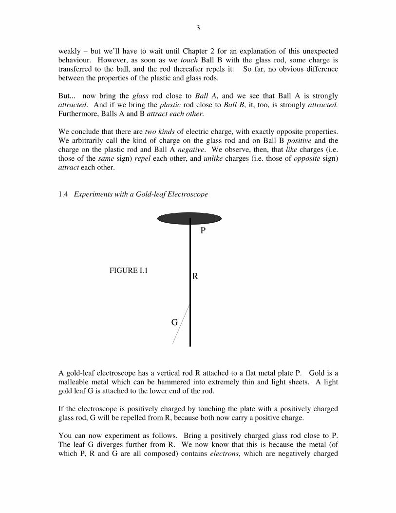
A gold-leaf electroscope has a vertical rod R attached to a flat metal plate P. Gold is a

malleable metal which can be hammered into extremely thin and light sheets. A light

gold leaf G is attached to the lower end of the rod.

If the electroscope is positively charged by touching the plate with a positively charged

glass rod, G will be repelled from R, because both now carry a positive charge.

You can now experiment as follows. Bring a positively charged glass rod close to P.

The leaf G diverges further from R. We now know that this is because the metal (of

which P, R and G are all composed) contains electrons, which are negatively charged

P

R

G

FIGURE I.1

4

particles that can move about more or less freely inside the metal. The approach of the

positively charged glass rod to P attracts electrons towards P, thus increasing the excess

positive charge on G and the bottom end of R. G therefore moves away from R.

If on the other hand you were to approach P with a negatively charged plastic rod,

electrons would be repelled from P down towards the bottom of the rod, thus reducing the

excess positive charge there. G therefore approaches R.

Now try another experiment. Start with the electroscope uncharged, with the gold leaf

hanging limply down. (This can be achieved by touching P briefly with your finger.)

Approach P with a negatively charged plastic rod, but don’t touch. The gold leaf

diverges from R. Now, briefly touch P with a finger of your free hand. Negatively

charged electrons run down through your body to ground (or earth). Don’t worry – you

won’t feel a thing. The gold leaf collapses, though by this time the electroscope bears a

positive charge, because it has lost some electrons through your body. Now remove the

plastic rod. The gold leaf diverges again. By means of the negatively charged plastic rod

and some deft work with your finger, you have induced a positive charge on the

electroscope. You can verify this by approaching P alternately with a plastic (negative)

or glass (positive) rod, and watch what happens to the gold leaf.

1.5 Coulomb’s Law

If you are interested in the history of physics, it is well worth reading about the important

experiments of Charles Coulomb in 1785. In these experiments he had a small fixed

metal sphere which he could charge with electricity, and a second metal sphere attached

to a vane suspended from a fine torsion thread. The two spheres were charged and,

because of the repulsive force between them, the vane twisted round at the end of the

torsion thread. By this means he was able to measure precisely the small forces between

the charges, and to determine how the force varied with the amount of charge and the

distance between them.

From these experiments resulted what is now known as Coulomb’s Law. Two electric

charges of like sign repel each other with a force that is proportional to the product of

their charges and inversely proportional to the square of the distance between them:

.2

21

r

QQF ∝ 1.5.1

Here Q1 and Q2 are the two charges and r is the distance between them.

We could in principle use any symbol we like for the constant of proportionality, but in

standard SI (Système International) practice, the constant of proportionality is written as

,4

1

πε so that Coulomb’s Law takes the form

5

.4

12

21

r

QQF

πε= 1.5.2

Here ε is called the permittivity of the medium in which the charges are situated, and it

varies from medium to medium. The permittivity of a vacuum (or of “free space”) is

given the symbol ε0. Media other than a vacuum have permittivities a little greater than

ε0. The permittivity of air is very little different from that of free space, and, unless

specified otherwise, I shall assume that all experiments described in this chapter are done

either in free space or in air, so that I shall write Coulomb’s Law as

.4

12

21

0 r

QQF

πε= 1.5.3

You may wonder – why the factor 4π? In fact it is very convenient to define the permittivity in this

manner, with 4π in the denominator, because, as we shall see, it will ensure that all formulas that describe

situations of spherical symmetry will include a 4π, formulas that describe situations of cylindrical

symmetry will include 2π, and no π will appear in formulas involving uniform fields. Some writers

(particularly those who favour cgs units) prefer to incorporate the 4π into the definition of the permittivity,

so that Coulomb’s law appears in the form ,)/( 2

021 rQQF ε= though it is standard SI practice to

define the permittivity as in equation 1.5.3. The permittivity defined by equation 1.5.3 is known as the

“rationalized” definition of the permittivity, and it results in much simpler formulas throughout

electromagnetic theory than the “unrationalized” definition.

The SI unit of charge is the coulomb, C. Unfortunately at this stage I cannot give you an

exact definition of the coulomb, although, if a current of 1 amp flows for a second, the

amount of electric charge that has flowed is 1 coulomb. This may at first seem to be very

clear, until you reflect that we have not yet defined what is meant by an amp, and that,

I’m afraid, will have to come in a much later chapter.

Until then, I can give you some small indications. For example, the charge on an electron

is about −1.6022 × 10−19

C, and the charge on a proton is about +1.6022 × 10−19

C. That

is to say, a collection of 6.24 × 1018

protons, if you could somehow bundle them all

together and stop them from flying apart, amounts to a charge of 1 C. A mole of protons

(i.e. 6.022 × 1023

protons) which would have a mass of about one gram, would have a

charge of 9.65 × 104 C, which is also called a faraday (which is not at all the same thing

as a farad).

[The current definition of the coulomb and the amp, which will be given in Chapter 6, requires some

knowledge of electromagnetism. However, it is likely that, in 2015, the coulomb will be redefined in such

a manner that the magnitude of the charge on a single electron is exactly 1.60217 % 10−19 C.]

The charges involved in our experiments with pith balls, glass rods and gold-leaf

electroscopes are very small in terms of coulombs, and are typically of the order of

nanocoulombs.

The permittivity of free space has the approximate value

6

.mNC108542.8 21212

0

−−−×=ε

Later on, when we know what is meant by a “farad”, we shall use the units F m−1

to

describe permittivity – but that will have to wait until section 5.2.

You may well ask how the permittivity of free space is measured. A brief answer might

be “by carrying out experiments similar to those of Coulomb”. However – and this is

rather a long story, which I shall not describe here – it turns out that since we today

define the metre by defining the speed of light, c, to be exactly 2.997 925 58 × 108 m s

−1,

the permittivity of free space has a defined value, given, in SI units, by

.104

2

7

0c

=πε

It is therefore not necessary to measure ε0 any more than it is necessary to measure c.

But that, as I say, is a long story.

[But if, as is likely, the new definition of the coulomb, referred to on the previous page, becomes official in

2015, ε0 will no longer have an exact defined value, but its measured value will be approximately 8.8542 % 10

−12 C

2 N

−1 m

−2. Many teaching laboratories run an undergraduate experiment in which students measure

the charge on a capacitor of known physical dimensions and a measured potential difference between the

plates, and this enables the measured value of ε0 to be calculated.]

From the point of view of dimensional analysis, electric charge cannot be expressed in

terms of M, L and T, but it has a dimension, Q, of its own. (This assertion is challenged

by some, but this is not the place to discuss the reasons. I may add a chapter, eventually,

discussing this point much later on.) We say that the dimensions of electric charge are Q.

Exercise: Show that the dimensions of permittivity are

[ε0] = M−1

L−3

T2

Q2.

I shall strongly advise the reader to work out and make a note of the dimensions of every

new electric or magnetic quantity as it is introduced.

Exercise: Calculate the magnitude of the force between two point charges of 1 C each

(that’s an enormous charge!) 1 m apart in vacuo.

The answer, of course, is 1/(4πε0), and that, as we have just seen, is c2/10

7 = 9 × 10

9 N,

which is equal to the weight of a mass of 9.2 × 105 tonnes or nearly a million tonnes.

Exercise: Calculate the ratio of the electrostatic to the gravitational force between two

electrons. The numbers you will need are: Q = 1.60 × 10−19

C, m = 9.11 × 10−31

kg, ε0

= 8.85 × 10−12

N m2 C

−2 , G = 6.67 × 10

−11 N m

2 kg

−2 .

7

The answer, which is independent of their distance apart, since both forces fall off

inversely as the square of the distance, is ),4/( 2

0

2GmQ πε (and you should verify that this

is dimensionless), and this comes to 4.2 × 1042

. This is the basis of the oft-heard

statement that electrical forces are 1042

times as strong as gravitational forces – but such a

statement out of context is rather meaningless. For example, the gravitational force

between Earth and Moon is much more than the electrostatic force (if any) between them,

and cosmologists could make a good case for saying that the strongest forces in the

Universe are gravitational.

The ratio of the permittivity of an insulating substance to the permittivity of free space is

its relative permittivity, also called its dielectric constant. The dielectric constants of

many commonly-encountered insulating substances are of order “a few”. That is,

somewhere between 2 and 10. Pure water has a dielectric constant of about 80, which is

quite high (but bear in mind that most water is far from pure and is not an insulator.)

Some special substances, known as ferroelectric substances, such as strontium titanate

SrTiO3, have dielectric constants of a few hundred.

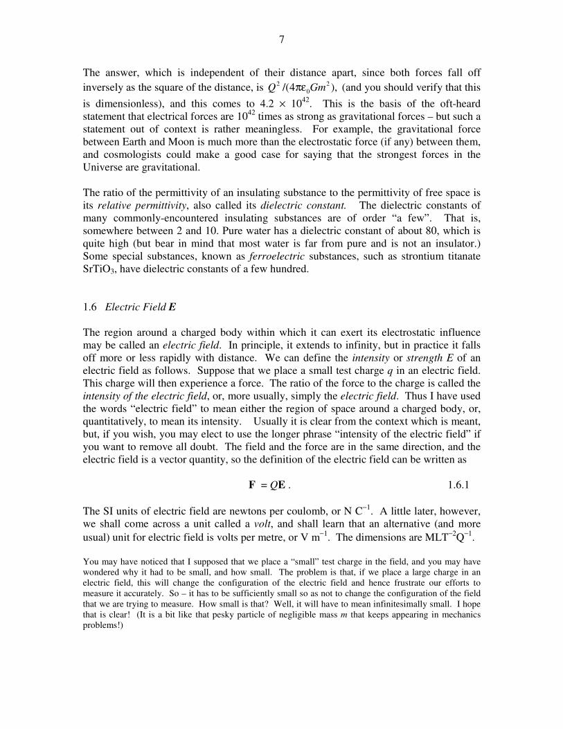
1.6 Electric Field E

The region around a charged body within which it can exert its electrostatic influence

may be called an electric field. In principle, it extends to infinity, but in practice it falls

off more or less rapidly with distance. We can define the intensity or strength E of an

electric field as follows. Suppose that we place a small test charge q in an electric field.

This charge will then experience a force. The ratio of the force to the charge is called the

intensity of the electric field, or, more usually, simply the electric field. Thus I have used

the words “electric field” to mean either the region of space around a charged body, or,

quantitatively, to mean its intensity. Usually it is clear from the context which is meant,

but, if you wish, you may elect to use the longer phrase “intensity of the electric field” if

you want to remove all doubt. The field and the force are in the same direction, and the

electric field is a vector quantity, so the definition of the electric field can be written as

F = QE . 1.6.1

The SI units of electric field are newtons per coulomb, or N C−1

. A little later, however,

we shall come across a unit called a volt, and shall learn that an alternative (and more

usual) unit for electric field is volts per metre, or V m−1

. The dimensions are MLT−2

Q−1

.

You may have noticed that I supposed that we place a “small” test charge in the field, and you may have

wondered why it had to be small, and how small. The problem is that, if we place a large charge in an

electric field, this will change the configuration of the electric field and hence frustrate our efforts to

measure it accurately. So – it has to be sufficiently small so as not to change the configuration of the field

that we are trying to measure. How small is that? Well, it will have to mean infinitesimally small. I hope

that is clear! (It is a bit like that pesky particle of negligible mass m that keeps appearing in mechanics

problems!)

8

We now need to calculate the intensity of an electric field in the vicinity of various

shapes and sizes of charged bodes, such as rods, discs, spheres, and so on.

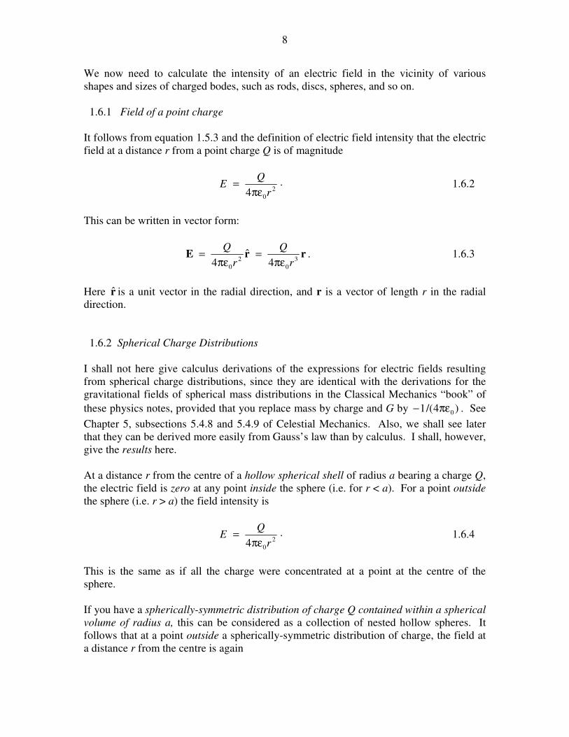
1.6.1 Field of a point charge

It follows from equation 1.5.3 and the definition of electric field intensity that the electric

field at a distance r from a point charge Q is of magnitude

.4 2

0r

QE

πε= 1.6.2

This can be written in vector form:

.4

ˆ4 3

0

2

0

r r

Q

r

Q

πε=

πε= rE 1.6.3

Here r̂ is a unit vector in the radial direction, and r is a vector of length r in the radial

direction.

1.6.2 Spherical Charge Distributions

I shall not here give calculus derivations of the expressions for electric fields resulting

from spherical charge distributions, since they are identical with the derivations for the

gravitational fields of spherical mass distributions in the Classical Mechanics “book” of

these physics notes, provided that you replace mass by charge and G by )4/(1 0πε− . See

Chapter 5, subsections 5.4.8 and 5.4.9 of Celestial Mechanics. Also, we shall see later

that they can be derived more easily from Gauss’s law than by calculus. I shall, however,

give the results here.

At a distance r from the centre of a hollow spherical shell of radius a bearing a charge Q,

the electric field is zero at any point inside the sphere (i.e. for r < a). For a point outside

the sphere (i.e. r > a) the field intensity is

.4 2

0r

QE

πε= 1.6.4

This is the same as if all the charge were concentrated at a point at the centre of the

sphere.

If you have a spherically-symmetric distribution of charge Q contained within a spherical

volume of radius a, this can be considered as a collection of nested hollow spheres. It

follows that at a point outside a spherically-symmetric distribution of charge, the field at

a distance r from the centre is again

9

.4 2

0r

QE

πε= 1.6.5

That is, it is the same as if all the charge were concentrated at the centre. However, at a

point inside the sphere, the charge beyond the distance r from the centre contributes zero

to the electric field; the electric field at a distance r from the centre is therefore just

.4 2

0r

QE r

πε= 1.6.6

Here Qr is the charge within a radius r. If the charge is uniformly distributed throughout

the sphere, this is related to the total charge by ,

3

Qa

rQr

= where Q is the total

charge. Therefore, for a uniform spherical charge distribution the field inside the sphere

is

.4 3

0a

QrE

πε= 1.6.7

That is to say, it increases linearly from centre to the surface, where it reaches a value of

,4 2

0a

Q

πε whereafter it decreases according to equation 1.6.5.

It is not difficult to imagine some electric charge distributed (uniformly or otherwise)

throughout a finite spherical volume, but, because like charges repel each other, it may

not be easy to realize this idealized situation in practice. In particular, if a metal sphere is

charged, since charge can flow freely through a metal, the self-repulsion of charges will

result in all the charge residing on the surface of the sphere, which then behaves as a

hollow spherical charge distribution with zero electric field within.

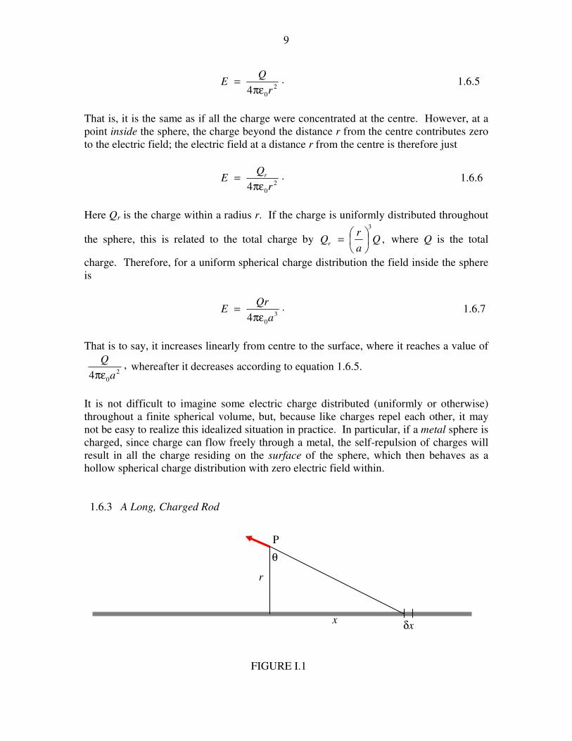
1.6.3 A Long, Charged Rod

r

x δx

θ

FIGURE I.1

P

10

A long rod bears a charge of λ coulombs per metre of its length. What is the strength of

the electric field at a point P at a distance r from the rod?

Consider an element δx of the rod at a distance 2/122 )( xr + from the rod. It bears a

charge λ δx. The contribution to the electric field at P from this element is

22

0

.4

1

xr

x

+

δλ

πεin the direction shown. The radial component of this is

.cos.4

122

0

θ+

δλ

πε xr

x But .secandsec,tan 22222 θ=+δθθ=δθ= rxrrxrx

Therefore the radial component of the field from the element δx is .cos4 0

δθθπε

λ

r To

find the radial component of the field from the entire rod, we integrate along the length of

the rod. If the rod is infinitely long (or if its length is much greater than r), we integrate

from θ = −π/2 to + π/2, or, what amounts to the same thing, from 0 to π/2, and double it.

Thus the radial component of the field is

.2

cos4

2

0

2/

00 rr

Eπε

λ=δθθ

πε

λ= ∫

π

1 6.8

The component of the field parallel to the rod, by considerations of symmetry, is zero, so

equation 1.6.8 gives the total field at a distance r from the rod, and it is directed radially

away from the rod.

Notice that equation 1.6.4 for a spherical charge distribution has 4πr2 in the denominator,

while equation 1.6.8, dealing with a problem of cylindrical symmetry, has 2πr.

11

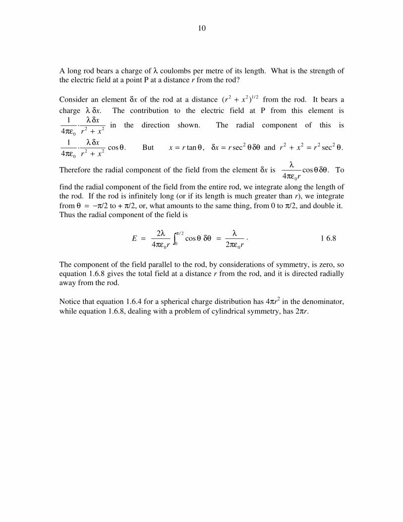
1.6.4 Field on the Axis of and in the Plane of a Charged Ring

Field on the axis of a charged ring.

Ring, radius a, charge Q. Field at P from element of charge δQ = .)(4 22

0 za

Q

+πε

δ

Vertical component of this = .)(4)(4

cos2/322

022

0 za

Qz

za

Q

+πε

δ=

+πε

θδ

Integrate for entire ring:

a

z

δQ

θ

P

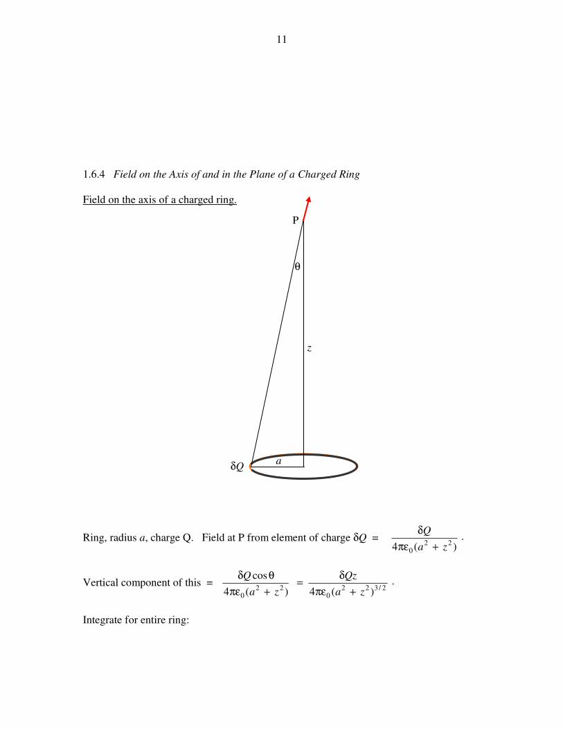
12

Field .)(4 2/322

0 za

zQE

+πε=

In terms of dimensionless variables:

,)1( 2/32

z

zE

+=

where E is in units of 2

04 a

Q

πε, and z is in units of a.

0 0.5 1 1.5 2 2.5 3 3.5 40

0.05

0.1

0.15

0.2

0.25

0.3

0.35

0.4

z

E

From calculus, we find that this reaches a maximum value of 3849.09

32=

at .7071.02/1 ==z

It reaches half of its maximum value where .9

3

)1( 2/32=

+ z

z

That is, 039723 32 =++− ZZZ , where .2zZ =

13

The two positive solution are Z = 0.041889 and 3.596267.

That is, .8964.1and2047.0=z

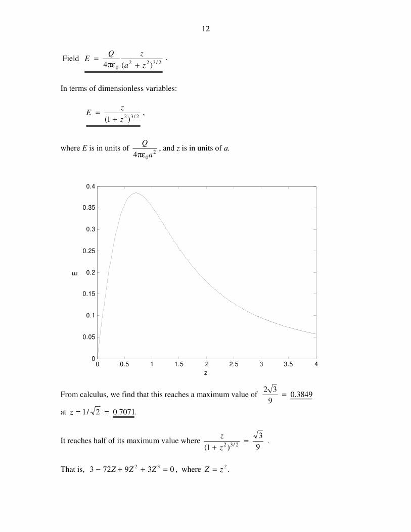
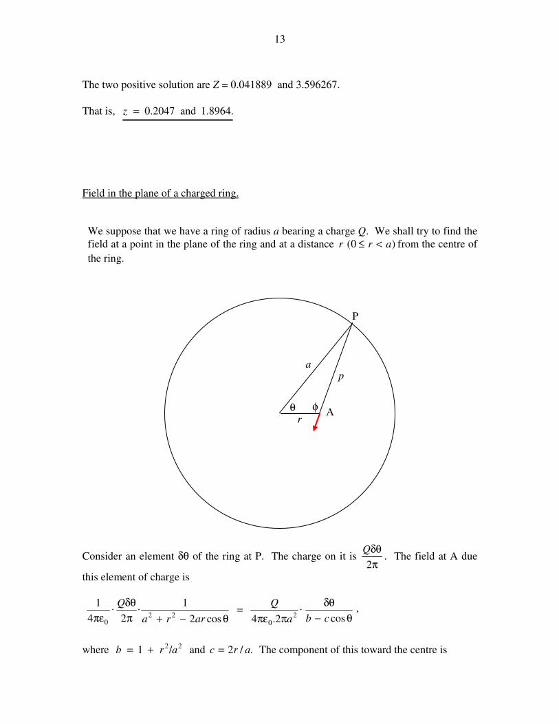
Field in the plane of a charged ring.

We suppose that we have a ring of radius a bearing a charge Q. We shall try to find the

field at a point in the plane of the ring and at a distance )0( arr <≤ from the centre of

the ring.

Consider an element δθ of the ring at P. The charge on it is π

δθ

2

Q. The field at A due

this element of charge is

,cos

.2.4cos2

1.2

.4

12

022

0 θ−

δθ

ππε=

θ−+π

δθ

πε cba

Q

arra

Q

where 22/1 arb += and ./2 arc = The component of this toward the centre is

θ A

P

a

r

φ

p

14

.cos

cos.2.4 2

0 θ−

δθφ

ππε−

cba

Q

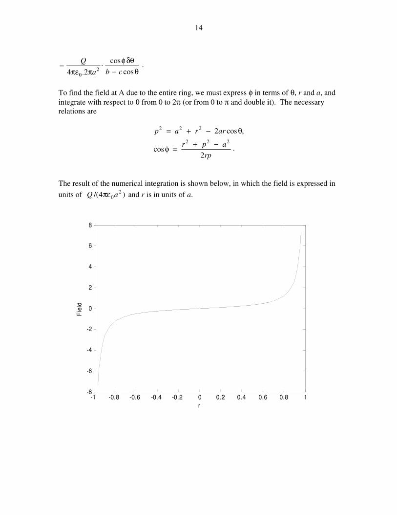
To find the field at A due to the entire ring, we must express φ in terms of θ, r and a, and

integrate with respect to θ from 0 to 2π (or from 0 to π and double it). The necessary

relations are

.2

cos

,cos2

222

222

rp

apr

arrap

−+=φ

θ−+=

The result of the numerical integration is shown below, in which the field is expressed in

units of )4/( 20aQ πε and r is in units of a.

-1 -0.8 -0.6 -0.4 -0.2 0 0.2 0.4 0.6 0.8 1-8

-6

-4

-2

0

2

4

6

8

r

Fie

ld

15

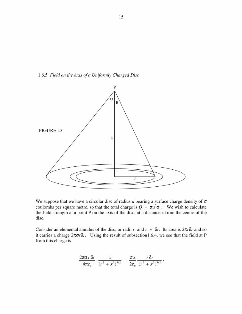
1.6.5 Field on the Axis of a Uniformly Charged Disc

We suppose that we have a circular disc of radius a bearing a surface charge density of σ

coulombs per square metre, so that the total charge is Q = πa2σ . We wish to calculate

the field strength at a point P on the axis of the disc, at a distance x from the centre of the

disc.

Consider an elemental annulus of the disc, or radii r and r + δr. Its area is 2πrδr and so

it carries a charge 2πσrδr. Using the result of subsection1.6.4, we see that the field at P

from this charge is

.)(

.2)(

.4

22/322

0

2/322

0 xr

rrx

xr

xrr

+

δ

ε

σ=

+πε

δπσ

α θ

x

P

r

FIGURE I.3

16

But .sec)(andsec,tan 2/1222 θ=+δθθ=δθ= xxrxrxr Thus the field from

the elemental annulus can be written

.sin2 0

δθθε

σ

The field from the entire disc is found by integrating this from θ = 0 to θ = α to obtain

.)(

12

)cos1(2 2/122

00

+−

ε

σ=α−

ε

σ=

xa

xE 1.6.11

This falls off monotonically from σ/(2ε0) just above the disc to zero at infinity.

1.6.6 Field of a Uniformly Charged Infinite Plane Sheet

All we have to do is to put α = π/2 in equation 1.6.10 to obtain

.2 0ε

σ=E 1.6.12

This is independent of the distance of P from the infinite charged sheet. The electric field

lines are uniform parallel lines extending to infinity.

Summary

Point charge Q: .4 2

0r

QE

πε=

Hollow Spherical Shell: E = zero inside the shell,

2

04 r

QE

πε= outside the shell.

Infinite charged rod: .2 0r

Eπε

λ=

Infinite plane sheet: .2 0ε

σ=E

17

1.7 Electric Field D

We have been assuming that all “experiments” described have been carried out in a

vacuum or (which is almost the same thing) in air. But what if the point charge, the

infinite rod and the infinite charged sheet of section 1.6 are all immersed in some medium

whose permittivity is not ε0, but is instead ε? In that case, the formulas for the field

become

.2

,2

,4 2 ε

σ

πε

λ

πε=

rr

QE

There is an ε in the denominator of each of these expressions. When dealing with media

with a permittivity other than ε0 it is often convenient to describe the electric field by

another vector, D, defined simply by

D = εE 1.7.1

In that case the above formulas for the field become just

.2

,2

,4 2

σ

π

λ

π=

rr

QD

The dimensions of D are Q L−2

, and the SI units are C m−2

.

This may seem to be rather trivial, but it does turn out to be more important than it may

seem at the moment.

Equation 1.7.1 would seem to imply that the electric field vectors E and D are just

vectors in the same direction, differing in magnitude only by the scalar quantity ε. This is

indeed the case in vacuo or in any isotropic medium – but it is more complicated in an

anisotropic medium such as, for example, an orthorhombic crystal. This is a crystal

shaped like a rectangular parallelepiped. If such a crystal is placed in an electric field,

the magnitude of the permittivity depends on whether the field is applied in the x- , the y-

or the z-direction. For a given magnitude of E, the resulting magnitude of D will be

different in these three situations. And, if the field E is not applied parallel to one of the

crystallographic axes, the resulting vector D will not be parallel to E. The permittivity in

equation 1.7.1 is a tensor with nine components, and, when applied to E it changes its

direction as well as its magnitude.

However, we shan’t dwell on that just yet, and, unless specified otherwise, we shall

always assume that we are dealing with a vacuum (in which case D = ε0E) or an isotropic

18

medium (in which case D = εE). In either case the permittivity is a scalar quantity and D

and E are in the same direction.

1.8 Flux

The product of electric field intensity and area is the flux ΦE. Whereas E is an intensive

quantity, ΦE is an extensive quantity. It dimensions are ML3T

−2Q

−1 and its SI units are N

m2 C

−1, although later on, after we have met the unit called the volt, we shall prefer to

express ΦE in V m.

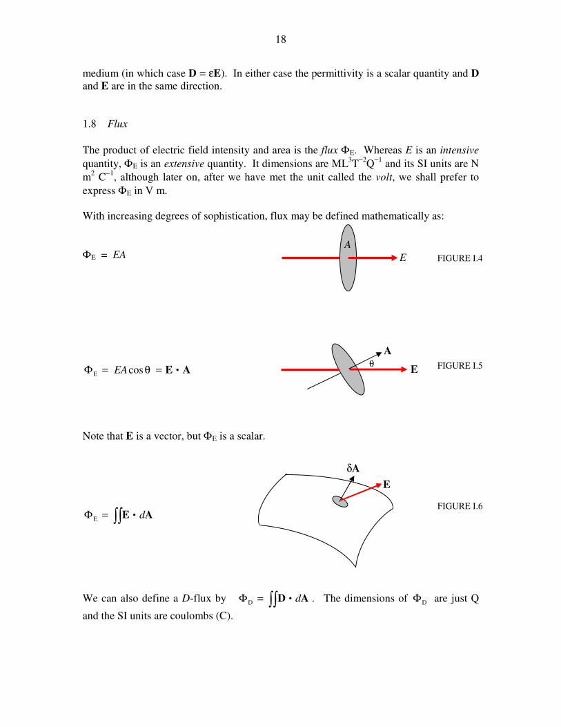
With increasing degrees of sophistication, flux may be defined mathematically as:

ΦE = EA

AE •=θ=Φ cosE EA

Note that E is a vector, but ΦE is a scalar.

∫∫ •=Φ AE dE

We can also define a D-flux by .D ∫∫ •=Φ AD d The dimensions of DΦ are just Q

and the SI units are coulombs (C).

A

E

E θ

A

δA

E

FIGURE I.4

FIGURE I.6

FIGURE I.5

19

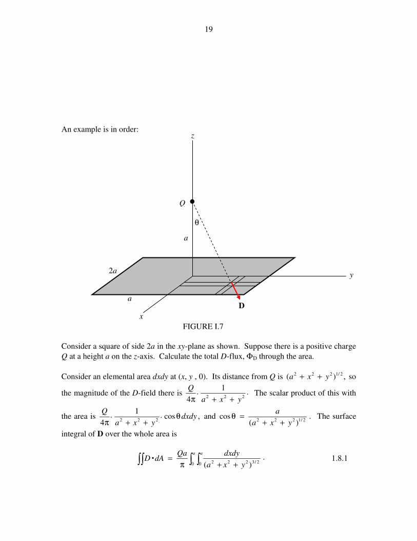
An example is in order:

Consider a square of side 2a in the xy-plane as shown. Suppose there is a positive charge

Q at a height a on the z-axis. Calculate the total D-flux, ΦD through the area.

Consider an elemental area dxdy at (x, y , 0). Its distance from Q is ,)( 2/1222 yxa ++ so

the magnitude of the D-field there is .1

.4 222

yxa

Q

++π The scalar product of this with

the area is ,cos.1

.4 222

dxdyyxa

Qθ

++π and .

)(cos

2/1222yxa

a

++=θ The surface

integral of D over the whole area is

.)(0 0 2/3222∫ ∫∫∫ ++π

=•a a

yxa

dxdyQadAD 1.8.1

x

y

z

θ

Q •

FIGURE I.7

a

a

2a

D

20

Now all we have to do is the nice and easy integral. Let ,tan22 ψ+= yax and the

inner integral ∫ ++

a

yxa

dx

0 2/3222 )( reduces, after some modest algebra, to

.2)( 2222

yaya

a

++ Thus we now have

.

2)(0 2222

2

∫∫∫++π

=•a

yaya

dyQadAD 1.8.2

With the further substitution ,sec222 ω=+ aya this reduces, after more careful

algebra, to

.6∫∫ =•Q

dAD 1.8.3

Two additional examples of calculating surface integrals may be found in Chapter 5,

section 5.6, of the Celestial Mechanics section of these notes. These deal with

gravitational fields, but they are essentially the same as the electrostatic case; just

substitute Q for m and −1/(4πε) for G.

I urge readers actually to go through the pain and the algebra and the trigonometry of

these three examples in order that they may appreciate all the more, in the next section,

the power of Gauss’s theorem.

1.9 Gauss’s Theorem

A point charge Q is at the centre of a sphere of radius r. Calculate the D-flux through the

sphere. Easy. The magnitude of D at a distance a is Q/(4πr2) and the surface area of the

sphere is 4πr2. Therefore the flux is just Q. Notice that this is independent of r; if you

double r, the area is four times as great, but D is only a quarter of what it was, so the total

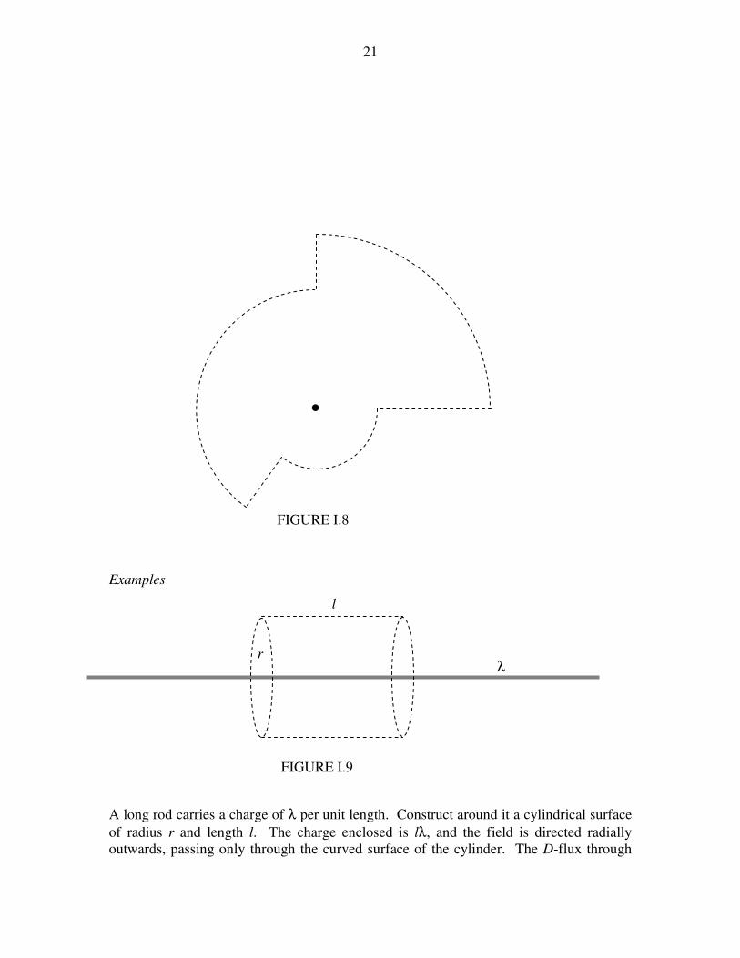
flux remains the same. You will probably agree that if the charge is surrounded by a

shape such as shown in figure I.8, which is made up of portions of spheres of different

radii, the D-flux through the surface is still just Q. And you can distort the surface as

much as you like, or you may consider any surface to be made up of an infinite number

of infinitesimal spherical caps, and you can put the charge anywhere you like inside the

surface, or indeed you can put as many charges inside as you like – you haven’t changed

the total normal component of the flux, which is still just Q. This is Gauss’s theorem,

which is a consequence of the inverse square nature of Coulomb’s law.

The total normal component of the D-flux through any closed surface is equal to the

charge enclosed by that surface.

21

Examples

A long rod carries a charge of λ per unit length. Construct around it a cylindrical surface

of radius r and length l. The charge enclosed is lλ, and the field is directed radially

outwards, passing only through the curved surface of the cylinder. The D-flux through

•

FIGURE I.8

r

l

FIGURE I.9

λ

22

the cylinder is lλ and the area of the curved surface is 2πrl, so D = lλ/(2πrl) and hence

).2/( rE πελ=

A flat plate carries a charge of σ per unit area. Construct around it a cylindrical surface

of cross-sectional area A. The charge enclosed by the cylinder is Aσ, so this is the D-flux

through the cylinder. It all goes through the two ends of the cylinder, which have a total

area 2A, and therefore D = σ/2 and E = σ/(2ε).

A hollow spherical shell of radius a carries a charge Q. Construct two gaussian spherical

surfaces, one of radius less than a and the other of radius r > a. The smaller of these two

surfaces has no charge inside it; therefore the flux through it is zero, and so E is zero.

The charge through the larger sphere is Q and is area is 4πr2. Therefore

.)4/(and)4/( 22 rQErQD πε=π= (It is worth going to Chapter 5 of Celestial

Mechanics, subsection 5.4.8, to go through the calculus derivation, so that you can

appreciate Gauss’s theorem all the more.)

A point charge Q is in the middle of a cylinder of radius a and length 2l. Calculate the

flux through the cylinder.

An infinite rod is charged with λ coulombs per unit length. It passes centrally through a

spherical surface of radius a. Calculate the flux through the spherical surface.

These problems are done by calculus in section 5.6 of Celestial Mechanics, and furnish

good examples of how to do surface integrals, and I recommend that you work through

them. However, it is obvious from Gauss’s theorem that the answers are just Q and 2aλ

respectively.

A point charge Q is in the middle of a cube of side 2a. The flux through the cube is, by

Gauss’s theorem, Q, and the flux through one face is Q/6. I hope you enjoyed doing this

by calculus in section 1.8.

A

σ

FIGURE I.10

23