chapter 16: consumption. john m. keynes: absolute income hypothesis consumption is a linear function...
TRANSCRIPT

Chapter 16: ConsumptionChapter 16: Consumption
John M. Keynes: Absolute Income Hypothesis
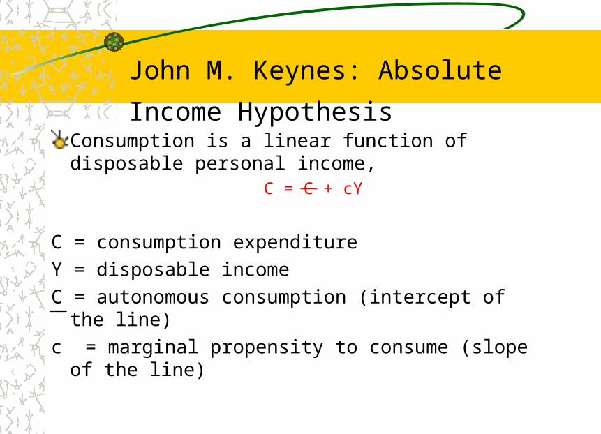
Consumption is a linear function of disposable personal income,
C = C + cY
C = consumption expenditureY = disposable incomeC = autonomous consumption (intercept of the line)c = marginal propensity to consume (slope of the line)
Properties of Consumption Function
Consumption is determined by current income
Marginal propensity to consume (MPC = ΔC/ΔY) is between zero and one (0<c<1)
Average propensity to consume (APC = C/Y) falls as income rises
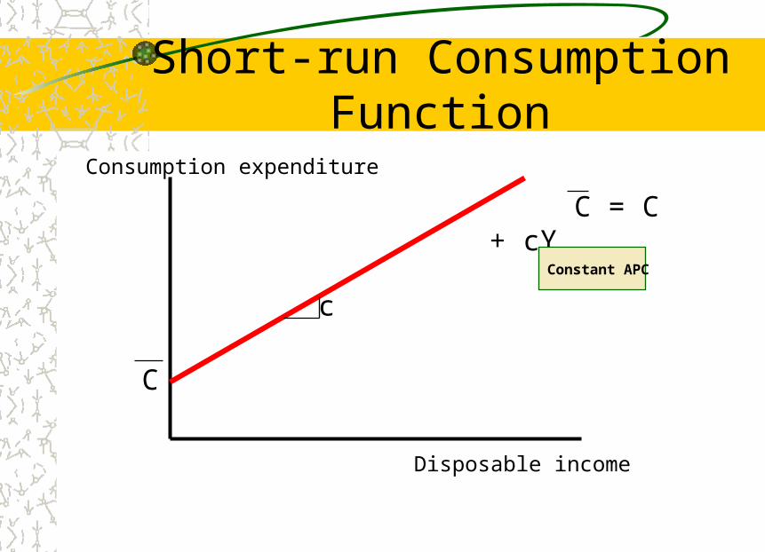
Short-run Consumption Function
Disposable income
Consumption expenditure
C = C + cY
C
c
Constant APC
Empirical Evidence
High income families have a higher marginal propensity to save (MPS = 1 – MPC)
High income families have a higher average propensity to save (APS = 1 – APC); APC falls with the level of income
In the long-run, autonomous consumption falls to zero (C = 0)
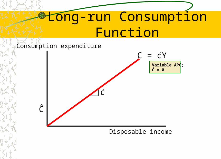
Long-run Consumption Function
C = ćY
Ĉ
ć
Variable APC; Ĉ = 0
Consumption expenditure
Disposable income

Irving Fisher: Intertemporal Choice
Consumption decisions are based on current and future income
Current period income = current income plus present value of future income: Y1 + Y2 / (1 + r), where r is a discount rate
Future period income = future income plus future value of current income: Y2 + (1 + r)Y1
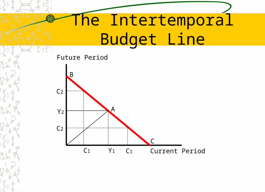
The Intertemporal Budget Line
A
B
C
Y1
Y2
C1
C2
C1
C2
Current Period
Future Period
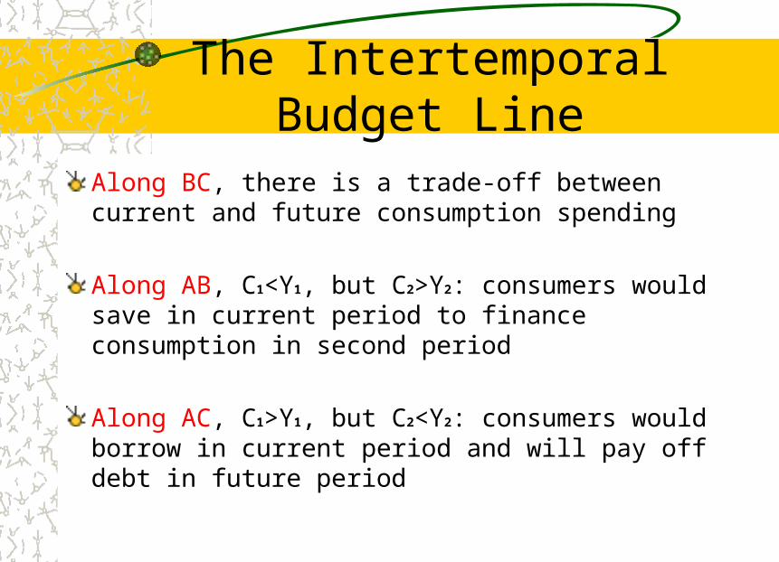
The Intertemporal Budget Line
Along BC, there is a trade-off between current and future consumption spending
Along AB, C1<Y1, but C2>Y2: consumers would save in current period to finance consumption in second period
Along AC, C1>Y1, but C2<Y2: consumers would borrow in current period and will pay off debt in future period
Consumer Preferences
Consumer preferences are shown by a family of indifference curves
Any combination of current and future consumption along an indifference curve provides the same level of satisfaction for the consumer
A higher indifference curve yields combinations with greater satisfaction
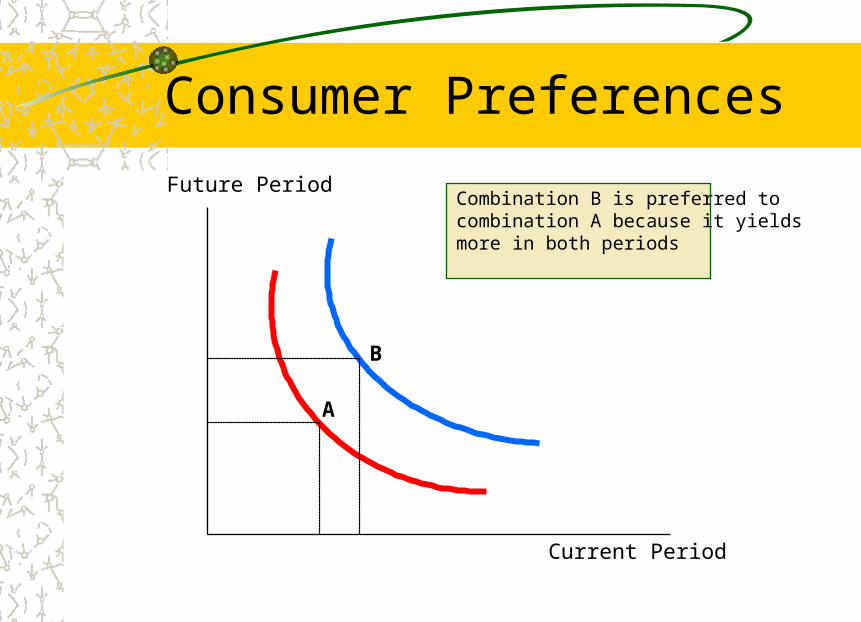
Consumer PreferencesFuture Period
Current Period
A
B
Combination B is preferred to combination A because it yields more in both periods
The Consumer’s Optimum
Consumer equilibrium is achieved at the tangency of the highest attainable indifference curve and the budget line
The tangency determines the optimum allocation of consumption spending in both periods; i.e. highest level of satisfaction within the budget

The Consumer’s Optimum
B
C1c
C1f
Future Period
Current Period
A
Higher income shifts the budget line up, positioning the consumer on a higher indifference curve and consumer’s optimum
C2f
C2c
Franco Modigliani: Life Cycle Hypothesis
Consumption depends on income and wealth
C = Consumption expenditureW = Consumer wealthR = Length of productive life timeT = Years of life
Consumption Function
C = (W + RY)/T = (1/T)W + (R/T)YDefine:
α = 1/T is the MPC out of wealthβ = R/T is the MPC out of income
C = αW + βY

Consumption Function
C = αW + βY
β
For the United States, α = 0.02 and β = 0.60.
1
αW
Consumption expenditure
Disposable income
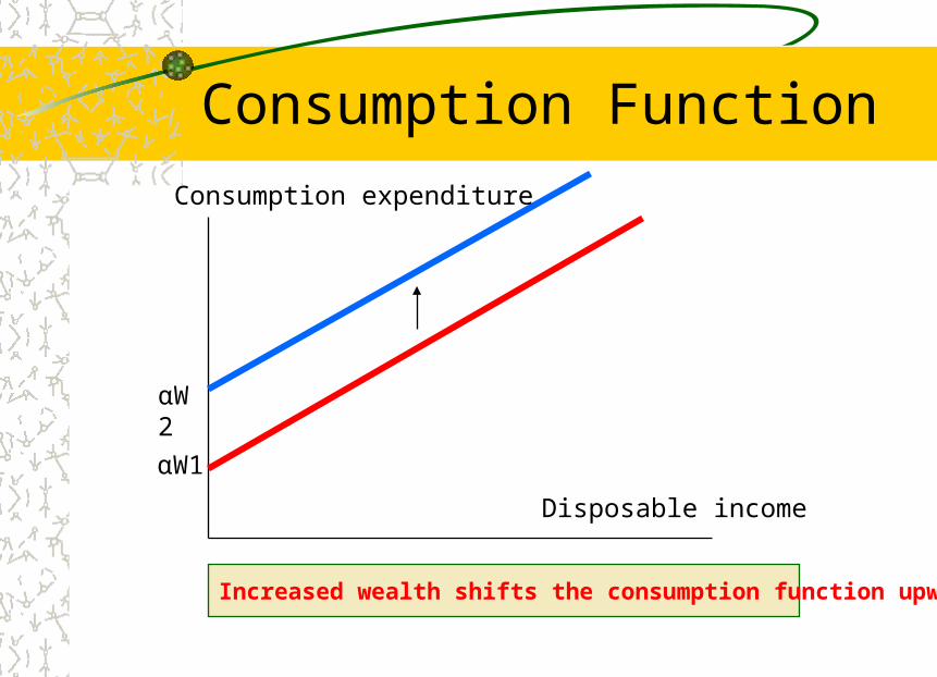
Consumption Function
Increased wealth shifts the consumption function upward.
αW1
αW2
Consumption expenditure
Disposable income

Consumer Behavior over Life Time
Consumption spending is a stable function of income
Consumers save their leftover income
Consumers accumulate wealth during the productive lifetime
Consumer finance retirement by dissaving and selling-off their assets
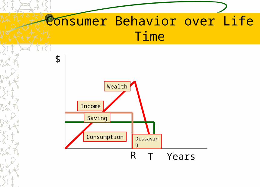
Consumer Behavior over Life Time
$
T
Wealth
Income
Consumption Dissaving
Saving
R Years

Milton Friedman: Permanent Income Hypothesis
Measured income consists of permanent and transitory income; Y = YP + YT
Permanent income is the average income we make during years of productive life
Transitory income is the random variation from the average
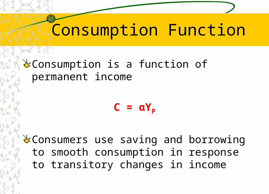
Consumption Function
Consumption is a function of permanent income
C = αYP
Consumers use saving and borrowing to smooth consumption in response to transitory changes in income
Determinants of Consumption
Combining all the theories, we can conclude that consumption depends on
Current incomeExpected future incomeWealthInterest rate