chapter 17 model command · chapter 17 718 because by statements are used to name the continuous...
TRANSCRIPT

MODEL Command
711
CHAPTER 17
MODEL COMMAND
In this chapter, the MODEL command is discussed. The MODEL
command is used to describe the model to be estimated. The first part of
this chapter describes the general modeling framework used by Mplus
and introduces a set of terms that are used to describe the model to be
estimated. The second part of this chapter explains how a model is
translated into the Mplus language using the options of the MODEL
command. The last part of the chapter describes variations of the
MODEL command. The MODEL command has variations for use with
models with indirect effects, models with linear and non-linear
constraints, models with parameter constraints for the Wald test,
multiple group models, mixture models, multilevel models, and models
for generating data for Monte Carlo simulation studies.
THE Mplus FRAMEWORK
VARIABLES
There are three important distinctions that need to be made about the
variables in an analysis in order to be able to specify a model. The
distinctions are whether variables are observed or latent, whether
variables are dependent or independent, and the scale of the observed
dependent variables.
OBSERVED OR LATENT VARIABLES
Two types of variables can be modeled: observed variables and latent
variables. Observed variables are variables that are directly measured
such as test scores and diagnostic criteria. They are sometimes referred
to as manifest variables, outcomes, or indicators. Latent variables are
variables that are not directly measured such as ability, depression, and
health status. They are measured indirectly by a set of observed
variables. There are two types of latent variables: continuous and
categorical. Continuous latent variables are sometimes referred to as
factors, dimension, constructs, or random effects. Categorical latent
variables are sometimes referred to as latent class variables or mixtures.
CHAPTER 17
712
DEPENDENT OR INDEPENDENT VARIABLES
Observed and latent variables can play the role of a dependent variable
or an independent variable in the model. The distinction between
dependent and independent variables is that of a regression analysis for y
regressed on x where y is a dependent variable and x is an independent
variable. An independent variable is one that is not influenced by any
other variable. Dependent variables are those that are influenced by
other variables. Other terms used for dependent variables are outcome
variable, response variable, indicator variable, y variable, and
endogenous variable. Other terms used for independent variables are
covariate, background variable, explanatory variable, predictor, x
variable, and exogenous variable.
SCALE OF OBSERVED DEPENDENT VARIABLES
The scale of observed dependent variables can be continuous, censored,
binary, ordered categorical (ordinal), unordered categorical (nominal),
counts, or combinations of these variable types.
UNDERLYING GENERAL MODEL
The purpose of modeling data is to describe the structure of a data set in
a simple way so that it is more understandable and interpretable.
Essentially, modeling data amounts to specifying a set of relationships
between variables.
The underlying model of Mplus consists of three parts: the measurement
model for the indicators of the continuous latent variables, the
measurement model for the indicators of the categorical latent variables,
and the structural model involving the continuous and categorical latent
variables and the observed variables that are not indicators of the
continuous or categorical latent variables. A model may consist of only
a measurement model as in confirmatory factor analysis or latent class
analysis, only a structural model as in a path analysis, or both a
measurement model and a structural model as in latent variable
structural equation modeling, longitudinal growth modeling, regression
mixture modeling, or growth mixture modeling.
MODEL Command
713
THE MODEL COMMAND
The MODEL command is used to describe the model to be estimated. It
has options for defining latent variables, describing relationships among
variables in the model, and specifying details of the model. The
MODEL command has variations for use with models with indirect
effects, models with non-linear constraints, models with parameter
constraints for the Wald test, multiple group models, mixture models,
multilevel models, and models for generating data for Monte Carlo
simulation studies.
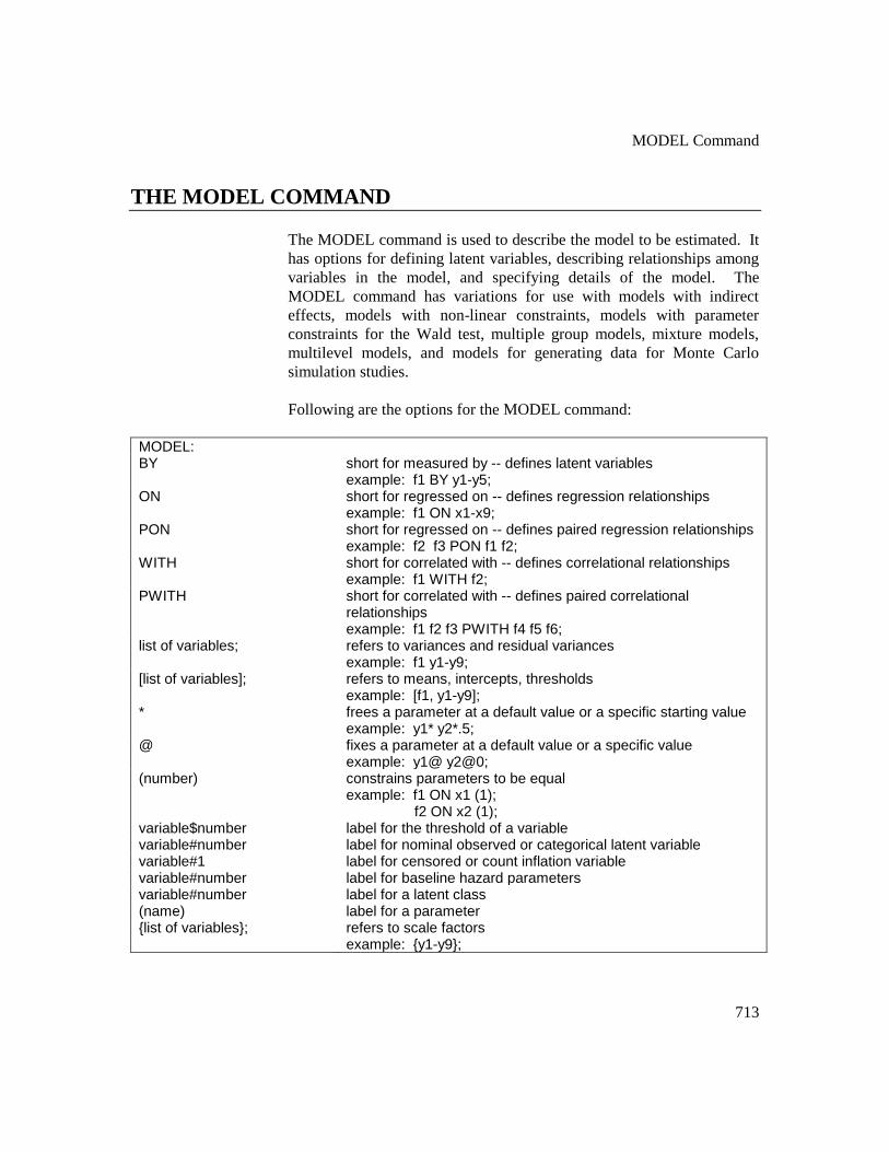
Following are the options for the MODEL command:
MODEL: BY short for measured by -- defines latent variables
example: f1 BY y1-y5; ON short for regressed on -- defines regression relationships
example: f1 ON x1-x9; PON short for regressed on -- defines paired regression relationships
example: f2 f3 PON f1 f2; WITH short for correlated with -- defines correlational relationships
example: f1 WITH f2; PWITH short for correlated with -- defines paired correlational
relationships example: f1 f2 f3 PWITH f4 f5 f6;
list of variables; refers to variances and residual variances example: f1 y1-y9;
[list of variables]; refers to means, intercepts, thresholds example: [f1, y1-y9];
* frees a parameter at a default value or a specific starting value example: y1* y2*.5;
@ fixes a parameter at a default value or a specific value example: y1@ y2@0;
(number) constrains parameters to be equal example: f1 ON x1 (1); f2 ON x2 (1);
variable$number label for the threshold of a variable variable#number label for nominal observed or categorical latent variable variable#1 label for censored or count inflation variable variable#number label for baseline hazard parameters variable#number label for a latent class (name) label for a parameter {list of variables}; refers to scale factors
example: {y1-y9};

CHAPTER 17
714
| growth model AT ON BY variable name XWITH
used for growth models, random effects, and latent variable interactions example: i s | y1@0 y2@1 y3@2; example: i s | y1 y2 y3 AT t1 t2 t3; example: s | y1 ON x1; example: s1 s2 s3 | f BY y1 y2 y3; f@1; example: logv | y; example: int | f1 XWITH f2;
MODEL INDIRECT: IND VIA MOD
describes indirect and total effects describes a specific indirect effect or a set of indirect effects when there is no moderation; describes a set of indirect effects that includes specific mediators; describes a specific indirect effect when there is moderation;
MODEL CONSTRAINT: NEW DO PLOT LOOP
describes linear and non-linear constraints on parameters assigns labels to parameters not in the analysis model; describes a do loop or double do loop; describes y-axis variables; describes x-axis variables;
MODEL TEST: DO
describes testing restrictions on the analysis model using the Wald test describes a do loop or double do loop;
MODEL PRIORS:
COVARIANCE DO
DIFFERENCE
specifies the prior distribution for the parameters assigns a prior to the covariance between two parameters; describes a do loop or double do loop; assigns priors to differences between parameters;
Following are variations of the MODEL command:
MODEL: describes the analysis model MODEL label: describes the group-specific model in multiple group analysis
and the model for each categorical latent variable and combinations of categorical latent variables in mixture modeling
MODEL: %OVERALL% %class label%
describes the overall part of a mixture model describes the class-specific part of a mixture model
MODEL: %WITHIN% %BETWEEN% %BETWEEN label%
describes the individual-level model describes the cluster-level model for a two-level model describes the cluster-level model for a three-level or cross-classified model
MODEL POPULATION: describes the data generation model MODEL POPULATION-label:
describes the group-specific data generation model in multiple group analysis and the data generation model for each categorical latent variable in mixture modeling

MODEL Command
715
MODEL POPULATION: %OVERALL% %class label%
describes the overall data generation model for a mixture model describes the class-specific data generation model for a mixture model
MODEL POPULATION: %WITHIN% %BETWEEN% %BETWEEN label%
describes the individual-level data generation model for a multilevel model describes the cluster-level data generation model for a two-level model describes the cluster-level data generation model for a three-level or cross-classified model
MODEL COVERAGE: describes the population parameter values for a Monte Carlo study
MODEL COVERAGE-label: describes the group-specific population parameter values in multiple group analysis and the population parameter values for each categorical latent variable and combinations of categorical latent variables in mixture modeling for a Monte Carlo study
MODEL COVERAGE: %OVERALL% %class label%
describes the overall population parameter values of a mixture model for a Monte Carlo study describes the class-specific population parameter values of a mixture model
MODEL COVERAGE: %WITHIN% %BETWEEN% %BETWEEN label%
describes the individual-level population parameter values for coverage describes the cluster-level population parameter values for a two-level model for coverage describes the cluster-level population parameter values for a three-level or cross-classified model for coverage
MODEL MISSING: describes the missing data generation model for a Monte Carlo study
MODEL MISSING-label: describes the group-specific missing data generation model for a Monte Carlo study
MODEL MISSING: %OVERALL% %class label%
describes the overall data generation model of a mixture model describes the class-specific data generation model of a mixture model
The MODEL command is required for all analyses except exploratory
factor analysis (EFA), exploratory latent class analysis (LCA), a baseline
model, and TYPE=BASIC.

CHAPTER 17
716
MODEL COMMAND OPTIONS There are three major options in the MODEL command that are used to
describe the relationships among observed variables and latent variables
in the model. They are:
BY
ON
WITH
BY is used to describe the regression relationships in the measurement
model for the indicators of the continuous latent variables. These
relationships define the continuous latent variables in the model. BY is
short for measured by. ON is used to describe the regression
relationships among the observed and latent variables in the model. It is
short for regressed on. WITH is used to describe correlational
(covariance) relationships in the measurement and structural models. It
is short for correlated with.
The model in the following figure is used to illustrate the use of the BY,
ON, and WITH options. The squares represent observed variables and
the circles represent latent variables. Regression relationships are
represented by arrows from independent variables to dependent
variables. The variables f1 and f2 are continuous latent variables. The
observed dependent variables are y1, y2, y3, y4, y5, y6, y7, y8, and y9.
The measurement part of the model consists of the two continuous latent
variables and their indicators. The continuous latent variable f1 is
measured by y1, y2, y3, y4, and y5. The continuous latent variable f2 is
measured by y6, y7, y8, and y9. The structural part of the model
consists of the regression of the two continuous latent variables on nine
observed independent variables. The observed independent variables are
x1, x2, x3, x4, x5, x6, x7, x8, and x9. Following is the MODEL
command for the figure below:
MODEL: f1 BY y1-y5;
f2 BY y6-y9;
f1 f2 ON x1-x9;

MODEL Command
717
BY The BY option is used to name and define the continuous latent
variables in the model. BY is short for measured by. The parameters
that are estimated are sometimes referred to as factor loadings or
lambdas. These are the coefficients for the regressions of the observed
dependent variables on the continuous latent variables. These observed
dependent variables are sometimes referred to as factor indicators. Each
BY statement can be thought of as a set of ON statements that describes
the regressions of a set of observed variables on a continuous latent
variable or factor. However, continuous latent variables in the
measurement model cannot be specified using a set of ON statements

CHAPTER 17
718
because BY statements are used to name the continuous latent variables.
BY statements also provide a set of convenient defaults.
Observed factor indicators for continuous latent variables can be
continuous, censored, binary, ordered categorical (ordinal), or counts.
Factor indicators can also be continuous latent variables or the inflation
part of censored and count variables. Combinations of all factor
indicator types are allowed. With TYPE=TWOLEVEL and
TYPE=TWOLEVEL MIXTURE, factor indicators for continuous latent
variables can be between-level random effects. These factor indicators
can appear only on the BETWEEN level.
CONFIRMATORY FACTOR ANALYSIS MODELING
In this section the use of the BY option for confirmatory factor analysis
(CFA) models is described. Following are the two BY statements that
describe how the continuous latent variables in the figure above are
measured:
f1 BY y1- y5;
f2 BY y6- y9;
The factor loading of any observed variable mentioned on the right-hand
side of the BY statement is free to be estimated with the exception of the
factor loading of the first variable after the BY option. This factor
loading is fixed at one as the default. Fixing a factor loading of an
indicator of a continuous latent variable sets the metric of the continuous
latent variable. Setting the metric can also be accomplished by fixing
the variance of the continuous latent variable to one and freeing the
factor loading of the factor indicator that is fixed at one as the default.
In the example above, the factor loadings of y1 and y6 are fixed at one.
The other factor loadings are estimated using default starting values of
one.
Following is an example of how to set the metric of the continuous latent
variable by fixing the variance of the continuous latent variable to one
and allowing all factor loadings to be free:
f1 BY y1* y2- y5;
f2 BY y6* y7- y9;
f1@1 f2@1;
MODEL Command
719
where the asterisk (*) after y1 and y6 frees the factor loadings of y1 and
y6, and the @1 after f1 and f2 fixes the variances of f1 and f2 to one.
The use of the asterisk (*); @ symbol; and the specification of means,
thresholds, variances, and covariances are discussed later in the chapter.
Residual variances are estimated as the default when factor indicators
are continuous or censored. Residual covariances among the factor
indicators are fixed at zero as the default. All default settings can be
overridden. How to do so is discussed later in this chapter.
The BY option can also be used to define continuous latent variables
underlying other continuous latent variables that have observed factor
indicators. This is referred to as second-order factor analysis. However,
a continuous latent variable cannot be used on the right-hand side of a
BY statement before it has been defined on the left-hand side of another
BY statement. For example, the following statements are acceptable:
f1 BY y1 y2 y3 y4 y5;
f2 BY y6 y7 y8 y9;
f3 BY f1 f2;
whereas, the following statements are not acceptable:
f3 BY f1 f2;
f1 BY y1 y2 y3 y4 y5;
f2 BY y6 y7 y8 y9;
because f1 and f2 are used on the right-hand side of a BY statement
before they are defined on the left-hand side of a BY statement.
EXPLORATORY STRUCTURAL EQUATION MODELING
In this section the use of the BY option for exploratory structural
equation (ESEM) modeling (Asparouhov & Muthén, 2009a) is
described. One of the differences between CFA and EFA factors is that
CFA factors are not rotated. For a set of EFA factors, the factor loading
matrix is rotated as in conventional EFA using the rotations available
through the ROTATION option of the ANALYSIS command. A set of
EFA factors must have the same factor indicators. A set of EFA factors
can be regressed on the same set of covariates. An observed or latent
variable can be regressed on a set of EFA factors. EFA factors are
CHAPTER 17
720
allowed with TYPE=GENERAL and TYPE=COMPLEX with observed
dependent variables that are continuous, censored, binary, ordered
categorical (ordinal), and combinations of these variable types. EFA
factors are not allowed when summary data are analyzed or when the
MLM, MLMV, or GLS estimators are used.
The BY option has three special features that are used with sets of EFA
factors in the MODEL command. One feature is used to define sets of
EFA factors. The second feature is a special way of specifying factor
loading matrix equality for sets of EFA factors. The third feature is used
in conjunction with the TARGET setting of the ROTATION option of
the ANALYSIS command to provide target factor loading values to
guide the rotation of the factor loading matrix for sets of EFA factors.
DEFINING EFA FACTORS
Following is an example of how to define a set of EFA factors using the
BY option:
f1-f2 BY y1-y5 (*1);
where the asterisk (*) followed by a label specifies that factors f1 and f2
are a set of EFA factors with factor indicators y1 through y5.
Following is an alternative specification:
f1 BY y1-y5 (*1);
f2 BY y1-y5 (*1);
where the label 1 specifies that factors f1 and f2 are part of the same set
of EFA factors. Rotation is carried out on the five by two factor loading
matrix. Labels for EFA factors must follow an asterisk (*). EFA factors
with the same label must have the same factor indicators.
More than one set of EFA factors may appear in the MODEL command.
For example,
f1-f2 BY y1-y5 (*1);
f3-f4 BY y6-y10 (*2);
MODEL Command
721
specifies that factors f1 and f2 are one set of EFA factors with the label
1 and factors f3 and f4 are another set of EFA factors with the label 2.
The two sets of EFA factors are rotated separately.
Factors in a set of EFA factors can be regressed on covariates but the set
of covariates must be the same, for example,
f1-f2 ON x1-x3;
or
f1 ON x1-x3;
f2 ON x1-x3;
A set of EFA factors can also be used as covariates in a regression, for
example,
y ON f1-f2;
EQUALITIES WITH EFA FACTORS
The BY option has a special convention for specifying equalities of the
factor loading matrices for more than one set of EFA factors. The
equality label is placed after the label that defines the set of EFA factors
and applies to the entire factor loading matrix not to a single parameter.
Following is an example of how to specify that the factor loading
matrices for the set of EFA factors f1 and f2 and the set of EFA factors
f3 and f4 are held equal:
f1-f2 BY y1-y5 (*1 1);
f3-f4 BY y6-y10 (*2 1);
The number 1 following the labels 1 and 2 that define the EFA factors
specifies that the factor loadings matrices for the two sets of EFA factors
are held equal.
TARGET ROTATION WITH EFA FACTORS
The BY option has a special feature that is used with the TARGET
setting of the ROTATION option of the ANALYSIS command to
specify target factor loading values for a set of EFA factors (Browne,

CHAPTER 17
722
2001). The target factor loading values are used to guide the rotation of
the factor loading matrix. Typically these values are zero. For the
TARGET rotation, a minimum number of target values must be given for
purposes of model identification. For the default oblique TARGET
rotation, the minimum is m(m-1) where the m is the number of factors.
For the orthogonal TARGET rotation, the minimum is m(m-1)/2. The
target values are given in the MODEL command using the tilde (~)
symbol. The target values are specified in a BY statement using the tilde
(~) symbol as follows:
f1 BY y1-y5 y1~0 (*1);
f2 BY y1-y5 y5~0 (*1);
where the target factor loading values for the factor indicator y1 for
factor f1 and y5 for factor f2 are zero.
ON
The ON option is used to describe the regression relationships in the
model and is short for regressed on. The general form of the ON
statement is:
y ON x;
where y is a dependent variable and x is an independent variable.
Dependent and independent variables can be observed or latent
variables.
In the previous figure, the structural relationships are the regressions of
the continuous latent variables f1 and f2 on the nine independent
variables x1 through x9. The ON statements shown below are used to
specify these regressions:
f1 ON x1-x9;
f2 ON x1-x9;
These statements specify that regression coefficients are free to be
estimated for f1 and f2 regressed on the independent variables x1
through x9 with default starting values of zero.
MODEL Command
723
For continuous latent variables, the residual variances are estimated as
the default. The residuals of the latent variables are correlated as the
default because residuals are correlated for latent variables that do not
influence any other variable in the model except their own indicators.
These defaults can be overridden. Means, variances, and covariances of
the independent variables in the model should not be mentioned in the
MODEL command because the model is estimated conditioned on the
covariates.
An ON statement can be used to describe the regression relationship
between an observed dependent variable and an observed independent
variable. Following is an example of how to specify the regression of an
observed dependent variable y9 on the observed independent variable
x9:
y9 ON x9;
The general form of the ON statement is used to describe regression
relationships for continuous latent variables and observed variables that
are continuous, censored, binary, ordered categorical (ordinal), counts,
censored inflated, and count inflated. The ON option has special
features for categorical latent variables and unordered categorical
(nominal) observed variables which are described below.
CATEGORICAL LATENT VARIABLES AND
UNORDERED CATEGORICAL (NOMINAL) OBSERVED
VARIABLES
For categorical latent variables and unordered categorical (nominal)
observed variables, the ON option is used to describe the multinomial
logistic regression of the categorical latent variable or the unordered
categorical (nominal) observed variable on one or more independent
variables.
For a categorical latent variable, an ON statement is specified for each
latent class except the last class which is the reference class. A class
label is used to refer to each class. Class labels use the convention of
adding to a variable name the number symbol (#) followed by a number.
For a categorical latent variable c with three classes,
c#1 c#2 ON x1-x3;
CHAPTER 17
724
specifies that regression coefficients are free to be estimated for classes
1 and 2 of the categorical latent variable c regressed on the independent
variables x1, x2, and x3. The intercepts in the regression of the
categorical latent variable on the independent variables are free to be
estimated as the default.
The statement above can be simplified to the following:
c ON x1-x3;
The multinomial logistic regression of one categorical latent variable on
another categorical latent variable where c2 has four classes and c1 has
three classes is specified as follows:
c2 ON c1;
or
c2#1 c2#2 c2#3 ON c1#1 c1#2;
For an unordered categorical (nominal) observed variable, an ON
statement is specified for each category except the last category which is
the reference category. A category label is used to refer to each
category. Category labels use the convention of adding to a variable
name the number symbol (#) followed by a number. For a three-
category variable u,
u#1 u#2 ON x1-x3;
specifies that regression coefficients are free to be estimated for
categories 1 and 2 of the unordered categorical (nominal) observed
variable u regressed on the independent variables x1, x2, and x3. The
thresholds in the regression of the unordered categorical (nominal)
observed variable on the independent variables are free to be estimated
as the default.
The statement above can be simplified to the following:
u ON x1-x3;

MODEL Command
725
Following is a table that describes how the relationships between
dependent variables and observed mediating variables or latent variables
are specified. Relationships with the designation of NA are not allowed.
Relationships not specified using the ON option are specified by listing
for each class the intercepts or thresholds in square brackets and the
residual variances with no brackets. Not shown in the table is that all
dependent variables can be regressed on independent variables that are
not mediating variables using the ON option.
Scale of
Dependent
Variable
Scale of Observed
Mediating Variable
Scale of Latent Variable
Continuous Censored,
Categorical,
and Count
Nominal Continuous Categorical Inflation
Part of
Censored
and Count
Continuous ON ON NA ON Mean and
variance vary
across classes
NA
Censored,
Categorical,
and Count
ON ON NA ON Mean/
threshold
and variance
vary across
classes
NA
Nominal ON ON NA ON Means vary
across classes
NA
Continuous
Latent
ON ON NA ON Mean and
variance vary
across classes
NA
Categorical
Latent
ON ON NA ON ON NA
Inflation
Part of
Censored
and Count
ON ON NA ON Mean varies
across classes
NA
PON
A second form of the ON option is PON. PON is used to describe the
paired regression relationships in the model and is short for regressed
on. PON pairs the variables on the left-hand side of the PON statement
with the variables on the right-hand side of the PON statement. For

CHAPTER 17
726
PON, the number of variables on the left-hand side of the PON statement
must equal the number of variables on the right-hand side of the PON
statement. For example,
y2 y3 y4 PON y1 y2 y3;
implies
y2 ON y1;
y3 ON y2;
y4 ON y3;
The PON option cannot be used with the simplified language for
categorical latent variables or unordered categorical (nominal) observed
variables.
WITH
The WITH option is used to describe correlational relationships in a
model and is short for correlated with. Correlational relationships
include covariances among continuous observed variables and
continuous latent variables and among categorical latent variables. With
the weighted least squares estimator, correlational relationships are also
allowed for binary, ordered categorical, and censored observed
variables. For all other variable types, the WITH option cannot be used
to specify correlational relationships. Special modeling needs to be used
in these situations, for example, using a latent variable that influences
both variables.
The NOCOVARIANCES setting of the MODEL option of the
ANALYSIS command specifies that the covariances and residual
covariances among all latent and observed variables in the analysis
model are fixed at zero. The WITH option is used to free selected
covariances and residual covariances.
Following is an example of how to specify the WITH option:
f1 WITH f2;
This statement frees the covariance parameter for the continuous latent
variables f1 and f2.

MODEL Command
727
Several variables can be included on both sides of the WITH statement.
In this situation, the variables on the left-hand side of the WITH
statement are crossed with the variables on the right-hand side of the
WITH statement resulting in all possible combinations of left- and right-
hand side variables.
The association between two categorical latent variables c1 and c2
where c1 has three classes and c2 has four classes is specified as
follows:
c1#1 c1#2 WITH c2#1 c2#2 c2#3;
The statement above can be simplified to:
c1 WITH c2;
The association coefficient for the last class of each categorical latent
variable is fixed at zero as the default as in loglinear modeling.
PWITH
A second form of the WITH option is PWITH. PWITH pairs the
variables on the left-hand side of the PWITH statement with those on the
right-hand side of the PWITH statement. For PWITH, the number of
variables on the left-hand side of the PWITH statement must equal the
number of variables on the right-hand side of the PWITH statement. For
example,
y1 y2 y3 PWITH y4 y5 y6;
implies
y1 WITH y4;
y2 WITH y5;
y3 WITH y6;
whereas,
y1 y2 y3 WITH y4 y5 y6;
implies
CHAPTER 17
728
y1 WITH y4;
y1 WITH y5;
y1 WITH y6;
y2 WITH y4;
y2 WITH y5;
y2 WITH y6;
y3 WITH y4;
y3 WITH y5;
y3 WITH y6;
The PWITH option cannot be used with the simplified language for
categorical latent variables.
VARIANCES/RESIDUAL VARIANCES
For convenience, no distinction is made in how variances and residual
variances are referred to in the MODEL command. The model defines
whether the parameter to be estimated is a variance or a residual
variance. Variances are estimated for independent variables and residual
variances are estimated for dependent variables. Variances of
continuous and censored observed variables and continuous latent
variables are free to be estimated as the default. Variances of categorical
observed variables are not estimated. When the Theta parameterization
is used in either a growth model or a multiple group model, variances for
continuous latent response variables for the categorical observed
variables are estimated. Unordered categorical (nominal) observed
variables, observed count variables, and categorical latent variables have
no variance parameters.
A list of observed or latent variables refers to the variances or residual
variances of those variables. For example,
y1 y2 y3;
refers to the variances of y1, y2, and y3 if they are independent variables
and refers to the residual variances of y1, y2, and y3 if they are
dependent variables. The statement means that the variances or residual
variances are free parameters to be estimated using default starting
values.
MODEL Command
729
MEANS/INTERCEPTS/THRESHOLDS
Means, intercepts, and thresholds are included in the analysis model as
the default. The NOMEANSTRUCTURE setting of the MODEL option
of the ANALYSIS command is used with TYPE=GENERAL to specify
that means, intercepts, and thresholds are not included in the analysis
model.
For convenience, no distinction is made in how means and intercepts are
referred to in the MODEL command. The model defines whether the
parameter to be estimated is a mean or an intercept. Means are
estimated for independent observed variables and observed variables that
are neither independent nor dependent variables in the model. Means for
nominal variables are logit coefficients corresponding to probabilities
for each category except the last category. Means for count variables are
log rates. Means for time-to-event variables in continuous-time survival
analysis are log rates. Means are also estimated for independent
continuous latent variables and independent categorical latent variables.
For an independent categorical latent variable, the means are logit
coefficients corresponding to probabilities for each class except the last
class.
Intercepts are estimated for continuous observed dependent variables,
censored observed dependent variables, unordered categorical (nominal)
observed dependent variable, count observed dependent variables,
baseline hazard parameters for continuous-time survival analysis,
continuous latent dependent variables, and categorical latent dependent
variables.
Thresholds are estimated for binary and ordered categorical observed
variables. The sign of a threshold is the opposite of the sign of a mean
or intercept for the same variable. For example, with a binary dependent
variable, a threshold of -0.5 is the same as an intercept of .5.
A list of observed or latent variables enclosed in brackets refers to
means, intercepts, or thresholds.
For example,
[y1 y2 y3];

CHAPTER 17
730
refers to the means of variables y1, y2, and y3 if they are independent
variables and refers to the intercepts if they are continuous dependent
variables. This statement indicates that the means or intercepts are free
parameters to be estimated using the default starting values.
If the variables are categorical, the thresholds are referred to as follows,
[y1$1 y1$2 y1$3 y2$1 y2$2];
where y1 is a four category variable with three thresholds and y2 is a
three category variable with two thresholds. y1$1 refers to the first and
lowest threshold of variable y1; y1$2 refers to the next threshold; and
y1$3 refers to the highest threshold. This statement means that the
thresholds are free parameters to be estimated using the default starting
values.
For models with a mean structure, all means, intercepts, and thresholds
of observed variables are free to be estimated at the default starting
values. The means and intercepts of continuous latent variables are
fixed at zero in a single group analysis. In a multiple group analysis, the
means and intercepts of the continuous latent variables are fixed at zero
in the first group and are free to be estimated in the other groups. In a
mixture model, the means and intercepts of the continuous latent
variables are fixed at zero in the last class and are free to be estimated in
the other classes. The means and intercepts of categorical latent
variables are fixed at zero in the last class and are free to be estimated in
the other classes.
CONVENIENCE FEATURES FOR THE MODEL
COMMAND
There are several features that make it easier for users to specify the
model to be estimated. One feature is the list function. A user can use a
hyphen to specify a list of variables, a list of equality constraints, and a
list of parameter labels.
When using the list function, it is important to know the order of
observed and latent variables that the program expects. The order of
observed variables is determined by the order of variables in the
NAMES or USEVARIABLES options of the VARIABLE command. If
MODEL Command
731
all of the variables in NAMES statement are used in the analysis, then
the order is taken from there. If the variables for the analysis are a
subset of the variables in the NAMES statement, the order is taken from
the USEVARIABLES statement.
The order of continuous latent variables is determined by the order of
the BY and | statements in the MODEL command. Factors defined using
the BY option come first in the order that they occur in the MODEL
command followed by the random effects defined using the | symbol in
the order that they occur in the MODEL command.
The list function can be used on the left- and right-hand sides of ON and
WITH statements and on the right-hand side of BY statements. A list on
the left-hand side implies multiple statements. A list on the right-hand
side implies a list of variables.
Following is an example of the use of the list function on the right-hand
side of a BY statement. It assumes the variables are in the order: y1, y2,
y3, y4, y5, y6, y7, y8, y9, y10, y11, and y12.
f1 BY y1-y4;
f2 BY y5-y9;
f3 BY y10-y12;
The program would interpret these BY statements as:
f1 BY y1 y2 y3 y4;
f2 BY y5 y6 y7 y8 y9;
f3 BY y10 y11 y12;
To use the list function with latent variables the order of latent variables
would be f1, f2, f3 because of the order of the BY statements in the
MODEL command.
Following is an example of using the list function on both the left- and
the right-hand sides of the ON statement:
f1-f3 ON x1-x3;
This implies the multiple statements:
CHAPTER 17
732
f1 ON x1 x2 x3;
f2 ON x1 x2 x3;
f3 ON x1 x2 x3;
The list function can also be used with the WITH option,
y1-y3 WITH y4-y6;
This implies
y1 WITH y4;
y1 WITH y5;
y1 WITH y6;
y2 WITH y4;
y2 WITH y5;
y2 WITH y6;
y3 WITH y4;
y3 WITH y5;
y3 WITH y6;
FREEING PARAMETERS AND ASSIGNING
STARTING VALUES
The asterisk (*) is used to free a parameter and/or assign a starting value
for the estimation of that parameter. It is placed after a parameter with a
number following it. For example:
y1*.5;
is interpreted as freeing the variance/residual variance of y1 to be
estimated with a starting value of 0.5.
Consider the BY statements from the previous section:
f1 BY y1 y2 y3 y4 y5;
f2 BY y6 y7 y8 y9;
As mentioned previously, the above statements result in the factor
loadings for y1 and y6 being fixed at one in order to set the metric of the
latent variables f1 and f2. All of the other parameters mentioned are free
MODEL Command
733
to be estimated with starting values of one. Consider the following BY
statements:
f1 BY y1* y2*0.5 y3 y4 y5;
f2 BY y6 y7-y9*0.9;
By putting an asterisk (*) after y1, the y1 parameter is freed at the
default starting value of one instead of being fixed at one by default. By
placing an asterisk (*) followed by 0.5 behind y2, the parameter starting
value is changed from the default starting value of 1 to 0.5. The
variables y3, y4, and y5 are free to be estimated at the default starting
value of one. In the BY statement for f2 the variables y7, y8, and y9 are
specified using the list function, y7-y9, followed by an asterisk (*) and
the value 0.9. This changes the starting values for y7, y8, and y9 from
the default starting value of 1 to 0.9.
These same features can be used with the ON and WITH options and for
assigning starting values to variances, means, thresholds, and scales.
Following are examples of assigning starting values to a variety of
parameters:
f1 ON x1-x3*1.5;
f1 WITH f2*.8;
y1-y12*.75;
[f1-f3*.5];
{y1-y12*5.0};
FIXING PARAMETER VALUES
In some cases, it is necessary to fix a parameter at a specific value. The
@ symbol is used to fix the values of parameters. Consider the
following example based on the measurement model in the earlier figure.
Following are the specifications needed to free the value of the first
indicator of each latent variable at starting values of one and to fix the
value of the second indicator of each latent variable to one in order to set
the metric of each latent variable:
f1 BY y1* y2@1 y3 y4 y5;
f2 BY y6* y7@1 y8 y9;
CHAPTER 17
734
By placing an asterisk (*) after y1, the factor loading for y1 is estimated
using the starting value of one. By placing @1 after y2, the factor
loading for y2 is fixed at one. Likewise, by placing an asterisk (*) after
y6, the factor loading for y6 is estimated using the starting value of one.
By placing @1 after y7, the factor loading for y7 is fixed at one.
The @ symbol can be used to fix any parameter in a model. The
following example fixes the covariance between f1 and f2 at zero:
f1 WITH f2@0;
CONSTRAINING PARAMETER VALUES TO BE
EQUAL
Parameters can be constrained to be equal by placing the same number in
parentheses following the parameters that are to be held equal. This
convention can be used for all parameters. Following is an example in
which regression coefficients, residual variances, and residual
covariances are held equal:
y1 ON x1 (1) ;
y2 ON x2 (1) ;
y3 ON x3 (1) ;
y1 y2 y3 (2);
y1 WITH y2-y3 (3);
In the above example, the regression coefficients for the three
regressions are constrained to be equal, the three residual variances are
constrained to be equal, and the two residual covariances are constrained
to be equal.
There can be only one number in parentheses on each line. If a
statement continues on more than one line, the number in parentheses
must be stated at the end of each line.
For example,
f1 BY y1 y2 y3 y4 y5 y6 y7 y8 y9 y10 y11 y12 (1)
y13 y14 y15 (1);

MODEL Command
735
specifies that the factor loadings of y2 through y15 are constrained to be
equal. The factor loading of y1 is fixed at one as the default.
The following statement,
f1 BY y1 y2 y3 y4 y5 y6 y7 y8 y9 y10 y11 y12
y13 y14 y15 (1);
specifies that the factor loadings of y13, y14, and y15 are constrained to
be equal because (1) refers to only the information on the line on which
it is located.
The following statement,
f1 BY y1 y2 y3 y4 y5 (1)
y6 y7 y8 y9 y10 (2)
y11 y12 y13 y14 y15 (3);
specifies that the factor loading of y1 is fixed at one and that the factor
loadings of y2, y3, y4, and y5 are held equal, that the factor loadings of
y6, y7, y8, y9, and y10 are held equal, and that the factor loadings of
y11, y12, y13, y14, and y15 are held equal.
Following are examples of how to constrain the parameters of means,
intercepts and/or thresholds to be equal.
[y1 y2 y3] (1);
indicates that the means/intercepts of variables y1, y2, and y3 are
constrained to be equal. The statements
[u1$1 u2$1 u3$1] (2);
[u1$2 u2$2 u3$2] (3);
[u1$3 u2$3 u3$3] (4);
indicate that the first threshold for variables u1, u2, and u3 are
constrained to be equal; that the second threshold for variables u1, u2,
and u3 are constrained to be equal; and that the third threshold for
variables u1, u2, and u3 are constrained to be equal. Out of nine
possible thresholds, three parameters are estimated. Only one set of
parentheses can be included on each line of the input file.
CHAPTER 17
736
USING THE LIST FUNCTION FOR ASSIGNING
STARTING VALUES, FIXING VALUES,
CONSTRAINING VALUES TO BE EQUAL, AND
ASSIGNING LABELS TO PARAMETERS
The list function is convenient for assigning starting values to
parameters, fixing parameters values, constraining parameter values to
be equal, and assigning labels to parameters.
ASSIGNING STARTING VALUES TO PARAMETERS
Following is an example of how to use the list function to assign starting
values to parameters:
f1 BY y1 y2-y4*0;
f2 BY y5 y6-y9*.5;
f3 BY y10 y11-y12*.75;
The program interprets these BY statements as:
f1 BY y1 y2*0 y3*0 y4*0;
f2 BY y5 y6*.5 y7*.5 y8*.5 y9*.5;
f3 BY y10 y11*.75 y12*.75;
where the starting value of 0 is assigned to the factor loadings for y2, y3,
and y4; the starting value of .5 is assigned to the factor loadings for y6,
y7, y8, and y9; and the starting value of .75 is assigned to the factor
loadings for y11 and y12. The factor loading for the first factor
indicator of each factor is fixed at one as the default to set the metric of
the factor.
FIXING PARAMETER VALUES
Following is an example of using the list function to fix parameter
values:
f1-f3@1;
The statement above fixes the variances/residual variances of f1, f2, and
f3 at one.

MODEL Command
737
CONSTRAINING PARAMETER VALUES TO BE EQUAL
Following is an example of using the list function to constrain parameter
values to be equal:
f1 BY y1-y5 (1)
y6-y10 (2);
The statement above specifies that the factor loadings of y2, y3, y4, and
y5 are held equal and that the factor loadings of y6, y7, y8, y9, and y10
are held equal. The factor loading of y1 is fixed at one as the default to
set the metric of the factor.
The list function can be used to assign equalities to a list of parameters
using a list of equality constraints. A list of equality constraints cannot
be used with a set of individual parameters. Following is an example of
how to use the list function with a list of parameters on the right-hand
side of the BY option:
f1 BY y1
y2-y5 (2-5);
f2 BY y6
y7-y10 (2-5);
The statements above specify that the factor loadings for y2 and y7 are
held equal, the factor loadings for y3 and y8 are held equal, the factor
loadings for y4 and y9 are held equal, and the factor loadings for y5 and
y10 are held equal. This can also be specified as shown below for
convenience.
f1 BY y1-y5 (1-5);
f2 BY y6-y10 (1-5);
No equality constraint is assigned to y1 and y6 even though they are part
of the list of variables because they are fixed at one to set the metric of
the factors. The number of equalities in the list must equal the number
of variables on the right-hand side of the BY option.
A list of equality constraints cannot be used with a list of parameters on
the left-hand side of an option. Following is an example of how equality

CHAPTER 17
738
constraints are specified for a list of parameters on the left-hand side of
the ON option:
y1-y3 ON x (1 2 3);
y4-y6 ON x (1 2 3);
where the regression coefficients in the regression of y1 on x and y4 on
x are constrained to be equal; the regression coefficients in the
regression of y2 on x and y5 on x are constrained to be equal; and the
regression coefficients in the regression of y3 on x and y6 on x are
constrained to be equal.
Following is an example of how equalities are specified when a list of
parameters appears on both the left- and right-hand sides of an option:
y1-y3 ON x1-x2 (1-2 3-4 5-6);
y4-y6 ON x1-x2 (1-2 3-4 5-6);
Each variable on the left-hand side of the ON option must have a list of
equalities for use with the variables on the right-hand side of the ON
option. Because there are three variables on the left-hand side of the ON
statement and two variables on the right-hand side of the ON statement,
three lists of two equalities are needed. A single list cannot be used.
Following is what this specifies:
y1 ON x1 (1);
y1 ON x2 (2);
y2 ON x1 (3);
y2 ON x2 (4);
y3 ON x1 (5);
y3 ON x2 (6);
y4 ON x1 (1);
y4 ON x2 (2);
y5 ON x1 (3);
y5 ON x2 (4);
y6 ON x1 (5);
y6 ON x2 (6);
The list function can be used with the simplified language for categorical
latent variables and unordered categorical (nominal) observed variables.

MODEL Command
739
The multinomial logistic regression of one categorical latent variable on
another categorical latent variable where c2 has four classes and c1 has
three classes is specified as follows:
c2 ON c1;
Following is an example of how equalities are specified when a list of
parameters appears on both the left- and right-hand sides of the ON
option using the simplified language:
c2 ON c1 (1-2 1-2 1-2);
or
c2 ON c1 (1-2);
Following is what this specifies:
c2#1 ON c1#1 (1);
c2#2 ON c1#2 (2);
c2#3 ON c1#1 (1);
c2#1 ON c1#2 (2);
c2#2 ON c1#1 (1);
c2#3 ON c1#3 (2);
ASSIGNING LABELS TO PARAMETERS
The list function can be used to assign labels to parameters in the
MODEL command. Following is an example of how to use the list
function in this way:
[y1-y5] (p1-p5);
The statement above assigns the parameter label p1 to y1, p2 to y2, p3 to
y3, p4 to y4, and p5 to y5.
The list function can be used to assign labels to a list of parameters using
a list of labels. A list of labels cannot be used with a set of individual
parameters. Following is an example of how to use the list function with
a list of parameters on the right-hand side of the BY option:
CHAPTER 17
740
f1 BY y1
y2-y5 (p2-p5);
The statement above assigns the label p2 to the factor loading for y2, p3
to the factor loading for y3, p4 to the factor loading for y4, and p5 to the
factor loading for y5.
A list of labels cannot be used with a list of parameters on the left-hand
side of an option. Following is an example of how labels are specified
for a list of parameters on the left-hand side of the ON option:
y1-y3 ON x (p1 p2 p3);
where the regression coefficient in the regression of y1 on x is assigned
the label p1; the regression coefficient in the regression of y2 on x is
assigned the label p; and the regression coefficient in the regression of
y3 on x is assigned the label p3.
Following is an example of how labels are specified when a list of
parameters appears on both the left- and right-hand sides of an option:
y1-y3 ON x1-x2 (p1-p2 p3-p4 p5-p6);
Each variable on the left-hand side of the ON option must have a list of
labels for use with the variables on the right-hand side of the ON option.
Because there are three variables on the left-hand side of the ON
statement and two variables on the right-hand side of the ON statement,
three lists of two equalities are needed. A single list cannot be used.
Because there are three variables on the left-hand side of the ON
statement and two variables on the right-hand side of the ON statement,
three lists of two equalities are needed.
Following is what this specifies:
y1 ON x1 (p1);
y1 ON x2 (p2);
y2 ON x1 (p3);
y2 ON x2 (p4);
y3 ON x1 (p5);
y3 ON x2 (p6);

MODEL Command
741
The list function can be used with the simplified language for categorical
latent variables and unordered categorical (nominal) observed variables.
The multinomial logistic regression of one categorical latent variable on
another categorical latent variable where c2 has four classes and c1 has
three classes is specified as follows:
c2 ON c1;
Following is an example of how labels are assigned when a list of
parameters appears on both the left- and right-hand sides of the ON
option using the simplified language:
c2 ON c1 (p1-p2 p3-p4 p5-p6);
Following is what this specifies:
c2#1 ON c1#1 (p1);
c2#2 ON c1#2 (p2);
c2#3 ON c1#1 (p3);
c2#1 ON c1#2 (p4);
c2#2 ON c1#1 (p5);
c2#3 ON c1#3 (p6);
SPECIAL LIST FUNCTION FEATURE
The list function has a special feature that can make model specification
easier. This feature allows a parameter to be mentioned in the MODEL
command more than once. The last specification is used in the analysis.
For example,
f1 BY y1-y6*0 y5*.5;
is interpreted by the program as
f1 BY y1*0 y2*0 y3*0 y4*0 y5*.5 y6*0;
Although y5 is assigned a starting value of 0.0 in the beginning of the
BY statement using the list function, y5 is assigned a starting value of
0.5 later in the statement. The program uses the last specification.

CHAPTER 17
742
If a variable is mentioned more than once on the right-hand side of a BY,
ON, or WITH statement or in a list of variances, means, or scale factors,
the program uses the last value it reads. This makes it convenient when
a user wants all of the starting values in a list to be the same except for a
few. The same feature can be used when fixing values. For example,
f1-f4@1 f3@2;
fixes the variances/residual variances of f1, f2, and f4 at one and fixes
the variance/residual variance of f3 at 2.
This feature can also be used with equalities, however, the variable from
the list that is not to be constrained to be equal must appear on a separate
line in the input file. In a line with an equality constraint, anything after
the equality constraint is ignored. For example,
f1 BY y1-y5 (1)
y4
y6-y10 (2);
indicates that the factor loadings for y2, y3, and y5 are held equal, the
factor loading for y4 is free and not equal to any other factor loading,
and the factor loadings for y6, y7, y8, y9, and y10 are held equal. The
factor loading for y1 is fixed at one as the default.
LABELING THRESHOLDS
For binary and ordered categorical dependent variables, thresholds are
referred to by using the convention of adding to a variable name a dollar
sign ($) followed by a number. The number of thresholds is equal to the
number of categories minus one. For example, if u1 is an ordered
categorical variable with four categories it has three thresholds. These
thresholds are referred to as u1$1, u1$2, and u1$3.
LABELING CATEGORICAL LATENT
VARIABLES AND UNORDERED CATEGORIAL
(NOMINAL) OBSERVED VARIABLES
The classes of categorical latent variables and the categories of
unordered categorical (nominal) observed variables are referred to by
MODEL Command
743
using the convention of adding to a variable name a number sign (#)
followed by the category/class number. For example, if c is a
categorical latent variable with three classes, the first two classes are
referred to as c#1 and c#2. The third class has all parameters fixed at
zero as a reference category. If u1 is a nominal variable with three
categories, the first two categories are referred to as u1#1 and u1#2. The
third category has all parameters fixed at zero as a reference category.
With the ON option categorical latent variables and unordered
categorical (nominal) observed variables can be referred to by their
variable name. With the WITH option, categorical latent variables can
be referred to by their variable name.
LABELING INFLATION VARIABLES
Censored and count inflation variables are referred to by using the
convention of adding to a variable name a number sign (#) followed by
the number one. For example, if y1 is a censored variable, the inflation
part of y1 is referred to as y1#1. If u1 is a count variable, the inflation
part of u1 is referred to as u1#1.
LABELING BASELINE HAZARD PARAMETERS
In continuous-time survival modeling, there are as many baseline hazard
parameters are there are time intervals plus one. When the
BASEHAZARD option of the ANALYSIS command is ON, these
parameters can be referred to by using the convention of adding to the
name of the time-to-event variable the number sign (#) followed by a
number. For example, for a time-to-event variable t with 5 time
intervals, the six baseline hazard parameters are referred to as t#1, t#2,
t#3, t#4, t#5, and t#6.
LABELING CLASSES OF A CATEGORICAL
LATENT VARIABLE
In the MODEL command, categorical latent variable classes are referred
to using labels. These labels are constructed by using the convention of
adding to the name of the categorical latent variable a number sign (#)
followed by a number. For example, if c is a categorical latent variable
with four classes, the labels for the four classes are c#1, c#2, and c#3.
The last class is the reference class.

CHAPTER 17
744
LABELING PARAMETERS
Labels can be assigned to parameters by placing a name in parentheses
following the parameter in the MODEL command. These labels are
used in three ways. First, they are used in conjunction with the MODEL
CONSTRAINT command to define linear and non-linear constraints on
the parameters in the model. Second, they are used with the MODEL
TEST command to test linear restrictions on the model defined in the
MODEL and MODEL CONSTRAINT commands. Third, they are used
with ESTIMATOR=BAYES and the MODEL PRIORS command to
specify the prior distribution for parameters in the MODEL command.
The parameter labels follow the same rules as variable names. They can
be up to 8 characters in length; must begin with a letter; can contain only
letters, numbers, and the underscore symbol; and are not case sensitive.
Only one label can appear on a line. Following is an example of how to
label parameters:
MODEL: y ON x1 (p1)
x2 (p2)
x3 (p3);
where p1 is the label assigned to the regression slope for y on x1, p2 is
the label assigned to the regression slope for y on the x2, and p3 is the
label assigned to the regression slope for y on x3.
The list function can be used to assign labels. Following is an example
of how to use the list function to label parameters:
MODEL: [y1-y10] (q1-q10);
y1-y10 (p1-p10);
f BY y1-y10 (z2-z10);
where the labels q1 through q10 are assigned to the intercepts of y1
through y10, the labels p1 through p10 are assigned to the residual
variances of y1 through y10, and the labels z2 through z10 are assigned
to the factors loadings for y2 through y10. The factor loading of y1 is
fixed at one as the default to set the metric of the factor.
If a list of labels is used, for example, in MODEL PRIORS, the order of
the labels is alphabetical not the order of the labels in the MODEL

MODEL Command
745
command. For example, the list p4-q2 includes p4, p5, p6, p7, p8, p9,
p10, q1, and q2.
The list function can be used with the ON and WITH options when there
are lists of variable names on both the right- and left-hand sides of these
options. Following is an example of how to use the list function to
assign labels when there are lists of variables on both the right- and left-
hand sides of ON:
y1-y3 ON x1-x2 (p1-p6);
The first variable on the left-hand side of ON is paired with all variables
on the right-hand side. Then the second variable on the left-hand side of
ON is paired with all variables on the right-hand side etc. The label p1
is assigned to the regression slope for y1 on x1. The label p2 is assigned
to the regression slope for y1 on x2. The label p3 is assigned to the
regression slope for y2 on y1. The label p6 is assigned to the regression
slope for y3 on x2.
Following is an example of how to use the list function to assign labels
when there are lists of variables on both the right- and left-hand sides of
WITH:
y1-y3 WITH y1-y3 ( p1-p3);
The labels are assigned to the upper triangle of a symmetric matrix read
row-wise. The label p1 is assigned to the covariance between y1 and y2.
The label p2 is assigned to the covariance between y1 and y3. The label
p3 is assigned to the covariance between y2 and y3.
SCALE FACTORS
In models that use TYPE=GENERAL, it may be useful to multiply each
observed variable or latent response variable by a scale factor that can be
estimated. For example, with categorical observed variables, a scale
factor refers to the underlying latent response variables and facilitates
growth modeling and multiple group analysis because the latent response
variables are not restricted to have across-time or across-group equalities
of variances. With continuous observed variables, using scale factors
containing standard deviations makes it possible to analyze a sample
covariance matrix by a correlation structure model.
CHAPTER 17
746
A list of observed variables in curly brackets refers to scale factors. For
example,
{u1 u2 u3};
refers to scale factors for variables u1, u2, and u3. This statement means
that the scale factors are free parameters to be estimated using the
default starting values of one.
The | SYMBOL
The | symbol is used to specify growth models, to name and define
random effect variables in the model, and to name and define latent
variable interactions.
GROWTH MODELS
Following is a description of the language specific to growth models.
The | symbol can be used with all analysis types to specify growth
models. The names on the left-hand side of the | symbol name the
random effect variables, also referred to as growth factors. The
statement on the right-hand side of the | symbol names the outcome and
specifies the time scores for the growth model.
Following is an example of the MODEL command for a quadratic
growth model for a continuous outcome specified without using the |
symbol:
MODEL: i BY y1-y4@1;
s BY y1@0 y2@1 y3@2 y4@3;
q BY y1@0 y2@1 y3@4 y4@9;
[y1-y4@0 i s q];
If the | symbol is used to specify the same growth model for a continuous
outcome, the MODEL command is:
MODEL: i s q | y1@0 y2@1 y3@2 y4@3;
All of the other specifications shown above are done as the default. The
defaults can be overridden by mentioning the parameters in the MODEL
command after the | statement. For example,

MODEL Command
747
MODEL: i s q | y1@0 y2@1 y3@2 y4@3;
[y1-y4] (1);
[i@0 s q];
changes the parameterization of the growth model from one with the
intercepts of the outcome variable fixed at zero and the growth factor
means free to be estimated to a parameterization with the intercepts of
the outcome variable held equal, the intercept growth factor mean fixed
at zero, and the slope growth factor means free to be estimated.
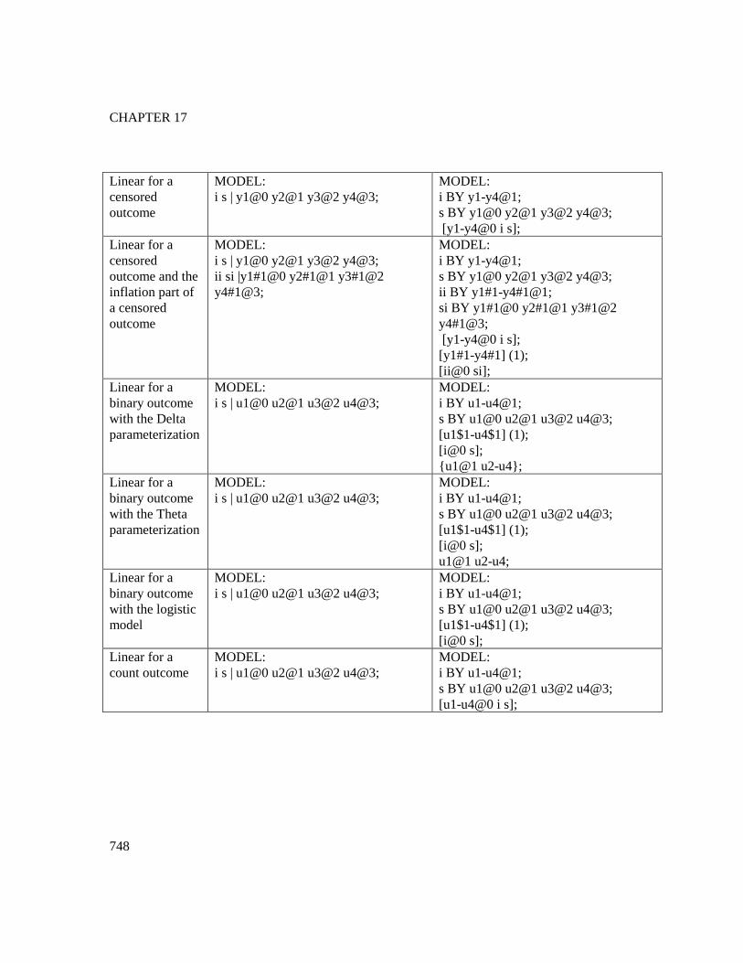
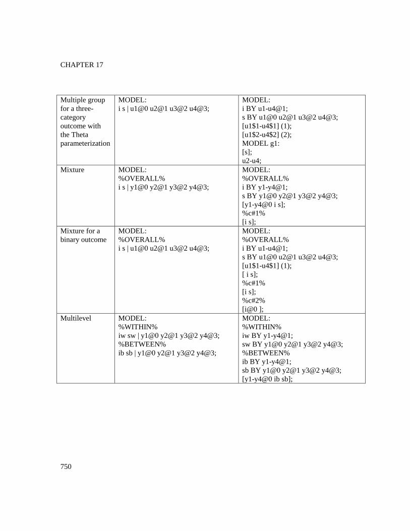
Many other types of growth models can be specified using the | symbol.
Following is a table that shows how to specify some of these growth
models using the | symbol and also how to specify the same growth
models using the BY option and other options. All examples are for
continuous outcomes unless specified otherwise.
Growth Language Alternative
Intercept only MODEL:
i | y1-y4@1;
MODEL:
i BY y1-y4@1;
[y1-y4@0 i];
Linear MODEL:
i s | y1@0 y2@1 y3@2 y4@3;
MODEL:
i BY y1-y4@1;
s BY y1@0 y2@1 y3@2 y4@3;
[y1-y4@0 i s];
Linear with free
time scores
MODEL:
i s | y1@0 y2@1 y3 y4;
MODEL:
i BY y1-y4@1;
s BY y1@0 y2@1 y3 y4;
[y1-y4@0 i s];
Quadratic MODEL:
i s q | y1@0 y2@1 y3@2 y4@3;
MODEL:
i BY y1-y4@1;
s BY y1@0 y2@1 y3@2 y4@3;
q BY y1@0 y2@1 y3@4 y4@9;
[y1-y4@0 i s q];
Piecewise MODEL:
i s1 | y1@0 y2@1 y3@2 y4@2 y5@2;
i s2 | y1@0 y2@0 y3@0 y4@1 y5@2;
MODEL:
i BY y1-y4@1;
s1 BY y1@0 y2@1 y3@2 y4@2 y5@2;
s2 BY y1@0 y2@0 y3@0 y4@1 y5@2;
[y1-y4@0 i s1 s2];
CHAPTER 17
748
Linear for a
censored
outcome
MODEL:
i s | y1@0 y2@1 y3@2 y4@3;
MODEL:
i BY y1-y4@1;
s BY y1@0 y2@1 y3@2 y4@3;
[y1-y4@0 i s];
Linear for a
censored
outcome and the
inflation part of
a censored
outcome
MODEL:
i s | y1@0 y2@1 y3@2 y4@3;
ii si |y1#1@0 y2#1@1 y3#1@2
y4#1@3;
MODEL:
i BY y1-y4@1;
s BY y1@0 y2@1 y3@2 y4@3;
ii BY y1#1-y4#1@1;
si BY y1#1@0 y2#1@1 y3#1@2
y4#1@3;
[y1-y4@0 i s];
[y1#1-y4#1] (1);
[ii@0 si];
Linear for a
binary outcome
with the Delta
parameterization
MODEL:
i s | u1@0 u2@1 u3@2 u4@3;
MODEL:
i BY u1-u4@1;
s BY u1@0 u2@1 u3@2 u4@3;
[u1$1-u4$1] (1);
[i@0 s];
{u1@1 u2-u4};
Linear for a
binary outcome
with the Theta
parameterization
MODEL:
i s | u1@0 u2@1 u3@2 u4@3;
MODEL:
i BY u1-u4@1;
s BY u1@0 u2@1 u3@2 u4@3;
[u1$1-u4$1] (1);
[i@0 s];
u1@1 u2-u4;
Linear for a
binary outcome
with the logistic
model
MODEL:
i s | u1@0 u2@1 u3@2 u4@3;
MODEL:
i BY u1-u4@1;
s BY u1@0 u2@1 u3@2 u4@3;
[u1$1-u4$1] (1);
[i@0 s];
Linear for a
count outcome
MODEL:
i s | u1@0 u2@1 u3@2 u4@3;
MODEL:
i BY u1-u4@1;
s BY u1@0 u2@1 u3@2 u4@3;
[u1-u4@0 i s];

MODEL Command
749
Linear for a
count outcome
and the inflation
part of a count
outcome
MODEL:
i s | u1@0 u2@1 u3@2 u4@3;
ii si | u1#1@0 u2#1@1 u3#1@2
u4#1@3;
MODEL:
i BY u1-u4@1;
s BY u1@0 u2@1 u3@2 u4@3;
ii BY u1#1-u4#1@1;
si BY u1#1@0 u2#1@1 u3#1@2
u4#1@3;
[u1-u4@0 i s];
[u1#1-u4#1] (1);
[ii@0 si];
Multiple group MODEL:
i s | y1@0 y2@1 y3@2 y4@3;
MODEL:
i BY y1-y4@1;
s BY y1@0 y2@1 y3@2 y4@3;
[y1-y4@0 i s];
MODEL g1:
[i s];
Multiple group
for a binary
outcome with
the Delta
parameterization
MODEL:
i s | u1@0 u2@1 u3@2 u4@3;
MODEL:
i BY u1-u4@1;
s BY u1@0 u2@1 u3@2 u4@3;
[u1$1-u4$1] (1);
{u1@1};
MODEL g1:
[s];
{u2-u4};
Multiple group
for a three-
category
outcome with
the Delta
parameterization
MODEL:
i s | u1@0 u2@1 u3@2 u4@3;
MODEL:
i BY u1-u4@1;
s BY u1@0 u2@1 u3@2 u4@3;
[u1$1-u4$1] (1);
[u1$2-u4$2] (2);
MODEL g1:
[s];
{u2-u4};
Multiple group
for a binary
outcome with
the Theta
parameterization
MODEL:
i s | u1@0 u2@1 u3@2 u4@3;
MODEL:
i BY u1-u4@1;
s BY u1@0 u2@1 u3@2 u4@3;
[u1$1-u4$1] (1);
u1@1;
MODEL g1:
[s];
u2-u4;
CHAPTER 17
750
Multiple group
for a three-
category
outcome with
the Theta
parameterization
MODEL:
i s | u1@0 u2@1 u3@2 u4@3;
MODEL:
i BY u1-u4@1;
s BY u1@0 u2@1 u3@2 u4@3;
[u1$1-u4$1] (1);
[u1$2-u4$2] (2);
MODEL g1:
[s];
u2-u4;
Mixture MODEL:
%OVERALL%
i s | y1@0 y2@1 y3@2 y4@3;
MODEL:
%OVERALL%
i BY y1-y4@1;
s BY y1@0 y2@1 y3@2 y4@3;
[y1-y4@0 i s];
%c#1%
[i s];
Mixture for a
binary outcome
MODEL:
%OVERALL%
i s | u1@0 u2@1 u3@2 u4@3;
MODEL:
%OVERALL%
i BY u1-u4@1;
s BY u1@0 u2@1 u3@2 u4@3;
[u1$1-u4$1] (1);
[ i s];
%c#1%
[i s];
%c#2%
[i@0 ];
Multilevel MODEL:
%WITHIN%
iw sw | y1@0 y2@1 y3@2 y4@3;
%BETWEEN%
ib sb | y1@0 y2@1 y3@2 y4@3;
MODEL:
%WITHIN%
iw BY y1-y4@1;
sw BY y1@0 y2@1 y3@2 y4@3;
%BETWEEN%
ib BY y1-y4@1;
sb BY y1@0 y2@1 y3@2 y4@3;
[y1-y4@0 ib sb];

MODEL Command
751
Multiple
indicator
MODEL:
f1 BY y11
y21 (1);
f2 BY y12
y22 (1);
f3 BY y13
y23 (1);
f4 BY y14
y24 (1);
[y11 y12 y13 y14] (2);
[y21 y22 y23 y24] (3);
i s | f1@0 f2@1 f3@2 f4@3;
MODEL:
f1 BY y11
y21 (1);
f2 BY y12
y22 (1);
f3 BY y13
y23 (1);
f4 BY y14
y24 (1);
[y11 y12 y13 y14] (2);
[y21 y22 y23 y24] (3);
i BY f1-f4@1;
s BY f1@0 f2@1 f3@2 f4@3;
[f1-f4@0 i@0 s];
Multiple
indicator for a
binary outcome
with the Delta
parameterization
MODEL:
f1 BY u11
u21 (1);
f2 BY u12
u22 (1);
f3 BY u13
u23 (1);
f4 BY u14
u24 (1);
[u11$1 u12$1 u13$1 u14$1] (2);
[u21$1 u22$1 u23$1 u24$1] (3);
{u11-u21@1 u12-u24};
i s | f1@0 f2@1 f3@2 f4@3;
MODEL:
f1 BY u11
u21 (1);
f2 BY u12
u22 (1);
f3 BY u13
u23 (1);
f4 BY u14
u24 (1);
[u11$1 u12$1 u13$1 u14$1] (2);
[u21$1 u22$1 u23$1 u24$1] (3);
{u11-u21@1 u12-u24};
i BY f1-f4@1;
s BY f1@0 f2@1 f3@2 f4@3;
[f1-f4@0 i@0 s];

CHAPTER 17
752
Multiple
indicator for a
binary outcome
with the Theta
parameterization
MODEL:
f1 BY u11
u21 (1);
f2 BY u12
u22 (1);
f3 BY u13
u23 (1);
f4 BY u14
u24 (1);
[u11$1 u12$1 u13$1 u14$1] (2);
[u21$1 u22$1 u23$1 u24$1] (3);
u11-u21@1 u12-u24;
i s | f1@0 f2@1 f3@2 f4@3;
MODEL:
f1 BY u11
u21 (1);
f2 BY u12
u22 (1);
f3 BY u13
u23 (1);
f4 BY u14
u24 (1);
[u11$1 u12$1 u13$1 u14$1] (2);
[u21$1 u22$1 u23$1 u24$1] (3);
u11-u21@1 u12-u24;
i BY f1-f4@1;
s BY f1@0 f2@1 f3@2 f4@3;
[f1-f4@0 i@0 s];
The defaults for the means/intercepts of the growth factors vary
depending on the scale of the outcome variable as described below. The
variances/residual variances and covariances/residual covariances of
growth factors are free to be estimated for all outcomes as the default.
For continuous, censored, and count outcomes, the means/intercepts of
the growth factors are free to be estimated. For a binary outcome, an
ordered categorical (ordinal) outcome, the inflation part of a censored
outcome, the inflation part of a count outcome, and a multiple indicator
growth model, the mean/intercept of the intercept growth factor is fixed
at zero. The means/intercepts of the slopes growth factors are free to be
estimated.
In multiple group analysis for continuous, censored, and count outcomes,
the means/intercepts of the growth factors are free to be estimated in all
groups. In multiple group analysis for a binary outcome, an ordered
categorical (ordinal) outcome, the inflation part of a censored outcome,
the inflation part of a count outcome, and a multiple indicator growth
model, the mean/intercept of the intercept growth factor is fixed at zero
in the first group and is free to be estimated in the other groups. The
means/intercepts of the slopes growth factors are free to be estimated in
all groups.
MODEL Command
753
In mixture models for continuous, censored, and count outcomes, the
means/intercepts of the growth factors are free to be estimated in all
classes. In mixture models for a binary outcome, an ordered categorical
(ordinal) outcome, the inflation part of a censored outcome, the inflation
part of a count outcome, and a multiple indicator growth model, the
mean/intercept of the intercept growth factor is fixed at zero in the last
class and is free to be estimated in the other classes. The
means/intercepts of the slopes growth factors are free to be estimated in
all classes.
The residual variances of continuous and censored outcome variables are
free as the default. The inflated part of censored outcomes, binary
outcomes, ordered categorical (ordinal) outcomes, count outcomes, and
the inflated part of count outcomes have no variance parameters. An
exception is the Theta parameterization used for binary and ordered
categorical (ordinal) outcomes. In the Theta parameterization, residual
variances are fixed at one at the first time point and are free at the other
time points.
AT
The AT option is used with TYPE=RANDOM to define a growth model
with individually-varying times of observation for the outcome variable.
AT is short for measured at. It is used in conjunction with the | symbol
to name and define the random effect variables in a growth model which
are referred to as growth factors.
Four types of growth models can be defined using AT and the | symbol:
an intercept only model, a model with two growth factors, a model with
three growth factors, and a model with four growth factors. The names
of the random effect variables are specified on the left-hand side of the |
symbol. The number of names determines which of the four models
model will be estimated. One name is needed for an intercept only
model and it refers to the intercept growth factor. Two names are
needed for a model with two growth factors: the first one is for the
intercept growth factor and the second one is for the slope growth factor
that uses the time scores to the power of one. Three names are needed
for a model with three growth factors: the first one is for the intercept
growth factor; the second one is for the slope growth factor that uses the
time scores to the power of one; and the third one is for the slope growth
factor that uses the time scores to the power of two. Four names are

CHAPTER 17
754
needed for a model with four growth factors: the first one is for the
intercept growth factor; the second one is for the slope growth factor that
uses the time scores to the power of one; the third one is for the slope
growth factor that uses the time scores to the power of two; and the
fourth one is for the slope growth factor that uses the time scores to the
power of three. Following are examples of how to specify these growth
models:
intercpt | y1 y2 y3 y4 AT t1 t2 t3 t4;
intercpt slope1 | y1 y2 y3 y4 AT t1 t2 t3 t4;
intercpt slope1 slope2 | y1 y2 y3 y4 AT t1 t2 t3 t4;
intercpt slope1 slope2 slope3 | y1 y2 y3 y4 AT t1 t2 t3 t4;
where intercpt, slope1, slope2, and slope3 are the names of the intercept
and slope growth factors; y1, y2, y3, and y4 are the outcome variables in
the growth model; and t1, t2, t3, and t4 are observed variables in the data
set that contain information on times of measurement. The TSCORES
option of the VARIABLE command is used to identify the variables that
contain information about individually-varying times of observation for
the outcome in a growth model. The variables on the left-hand side of
AT are paired with the variables on the right-hand side of AT.
The intercepts of the outcome variables are fixed at zero as the default.
The residual variances of the outcome variables are free to be estimated
as the default. The residual covariances of the outcome variables are
fixed at zero as the default. The means, variances, and covariances of
the intercept and slope growth factors are free as the default.
RANDOM SLOPES
The | symbol is used in conjunction with TYPE=RANDOM to name and
define the random slope variables in the model. The name on the left-
hand side of the | symbol names the random slope variable. The
statement on the right-hand side of the | symbol defines the random slope
variable. Random slopes are defined using the ON or PON options. ON
or PON statements used on the right-hand side of the | symbol may not
use the asterisk (*) or @ symbols. Otherwise, the regular rules regarding
ON and PON apply. The means and the variances of the random slope
variables are free as the default. Covariances among random slope
variables are fixed at zero as the default. Covariances between random

MODEL Command
755
slope variables and growth factors, latent variables defined using BY
statements, and observed variables are fixed at zero as the default.
With TYPE=TWOLEVEL RANDOM and TYPE=CROSSCLASSIFIED
RANDOM, the random slope variables are named and defined in the
within part of the MODEL command and used in the between part of the
MODEL command. For TYPE=THREELEVEL RANDOM, the random
slope variables are named and defined in the within and between level 2
parts of the MODEL command. Random slope variables defined in
within part of the MODEL command can be used in both the between
level 2 and between level 3 parts of the MODEL command. Random
slope variables defined in the between level 2 part of the MODEL
command can be used only in the between level 3 part of the MODEL
command.
For TYPE=THREELEVEL and TYPE=CROSSCLASSIFIED, random
slope variables are between-level variables. For TYPE=TWOLEVEL,
random slope variables are between-level variables unless specifically
designated as having variation on both levels. This is done by placing an
asterisk (*) after the name on the left-hand side of the | symbol as
follows:
s* | y ON x;
where the asterisk (*) indicates that the random slope variable s has
variation on both the within and between levels.
Following is an example of how to specify a random slope using the |
symbol:
s | y ON x;
where s is a random slope in the regression of y on x where y is a
continuous dependent variable and x is an independent variable. Both
dependent and independent variables can be latent or observed variables.
Lists can be used on both the left-hand side of the | symbol and the left-
and right-hand sides of ON and PON. Following is an example of how
to specify a set of random slopes using the | symbol and PON:
s1-s3 | y1-y3 PON x1-x3;

CHAPTER 17
756
where s1, s2, and s3 are random slopes in the regressions of y1 on x1, y2
on x2, and y3 on x3.
A random slope variable can refer to more than one slope by being used
on the left-hand side of more than one | statement. In this case, the
random slope variables are the same. For example,
s1 | y1 ON x1;
s1 | y2 ON x2;
defines the random slope, s1, to be the same in the regressions of y1 on
x1 and y2 on x2.
Another example is,
s2 | y1 ON x1 x2;
which defines the random slope, s2, to be the same in the regressions of
y1 on x1 and y1 on x2.
RANDOM FACTOR LOADINGS
For TYPE=TWOLEVEL and TYPE=CROSSCLASSIFIED, the | symbol
is used in conjunction with TYPE=RANDOM to name and define the
random factor loading variables in the model. The names on the left-
hand side of the | symbol name the random factor loading variables. The
statements on the right-hand side of the | symbol define the random
factor loading variables. Random factor loadings are defined using the
BY option. BY statements used on the right-hand side of the | symbol
may not use the asterisk (*) or @ symbol. Otherwise, the regular rules
regarding BY apply. The means and the variances of the random factor
loading variables are free as the default. Covariances between random
factor loading variables and growth factors, latent variables defined
using BY statements, and observed variables are fixed at zero as the
default.
For TYPE=TWOLEVEL, the random factor loading variables are named
and defined in the within part of the MODEL command and used in the
between part of the MODEL command. For
TYPE=CROSSCLASSIFIED, random factor loading variables that are
named and defined in the level 2a part of the MODEL command can be
MODEL Command
757
used in the level 2b part of the MODEL command. Level 2a is the
second cluster variable on the CLUSTER statement. Level 2b is the first
cluster variable on the CLUSTER statement. Random factor loading
variables are between-level variables. Following is an example of how
to specify random factor loadings using the | symbol:
s1-s10 | f BY y1-y10;
f@1;
where s1 through s10 are random factor loadings for the factor f. All
factor loadings are free. The metric of the factor is set by fixing the
factor variance to one.
RANDOM VARIANCES
The | symbol is used in conjunction with TYPE=RANDOM to name and
define random variance variables in the model. Random variances are
available only for TYPE=TWOLEVEL with ESTIMATOR=BAYES.
The name on the left-hand side of the | symbol names the random
variance variable. The variable on the right-hand side of the | symbol
specifies the variable that will have a random variance. The log of the
random residual variance is used in the model. The asterisk (*) or @
symbols may not be used on the right-hand side of the | symbol. The
means and the variances of the random variance variables are free as the
default. Covariances among random variance variables are fixed at zero
as the default. Covariances among random variance variables and
growth factors, latent variables defined using BY statements, and
observed variables are fixed at zero as the default. Following is an
example of how to specify and random variance using the | symbol.
logv | y;
where logv is the random variance for the variable y.
XWITH
The XWITH option is used with TYPE=RANDOM to define
interactions between continuous latent variables or between a continuous
latent variable and an observed variable. XWITH is short for multiplied
with. It is used in conjunction with the | symbol to name and define
interaction variables in a model. It is not available for
CHAPTER 17
758
TYPE=THREELEVEL or TYPE=CROSSCLASSIFIED. Following is
an example of how to use XWITH and the | symbol to name and define
an interaction:
int | f1 XWITH f2;
where int is the name of the interaction between f1 and f2. Interaction
variables can be used only on the right-hand side of ON statements.
The XWITH option can be used to create an interaction variable that is
the square of a latent variable. Following is an example of how this is
specified:
fsquare | f XWITH f;
Latent variable interactions are estimated using maximum likelihood for
all regular models as well as mixture models and multilevel models.
Interactions are allowed between continuous latent variables and
between a continuous latent variable and an observed variable. Factor
indicators for the continuous latent variables can be continuous,
censored, binary, ordered categorical (ordinal), counts, or combinations
of these variable types. Observed variables in the interaction can be
independent or mediating variables and the mediating variables can be
censored, binary, ordered categorical (ordinal), counts, or combinations
of these variable types. Dependent observed variables in the interaction
can have missing data. In many cases, numerical integration is required
in the maximum likelihood estimation of latent variable interactions.
Numerical integration becomes increasingly more computationally
demanding as the number of factors and the sample size increase.
Interactions between observed variables are handled using the DEFINE
command where an interaction variable is created via multiplication. If
an observed dependent variable has missing data, a latent variable can be
created for this observed variable and the procedure described above can
be used.
Interactions between categorical latent variables and between a
categorical latent variable and an observed or continuous latent variable
are handled using mixture modeling.
MODEL Command
759
Following is a table that summarizes ways of obtaining interactions for
different variable types.
Types of Variables Interaction Options
observed continuous with
observed continuous
DEFINE
observed categorical with
observed continuous
DEFINE
Multiple Group
observed continuous with
continuous latent
XWITH
observed categorical with
continuous latent
XWITH
Multiple Group
observed continuous with
categorical latent
MIXTURE
observed categorical with
categorical latent
MIXTURE
KNOWNCLASS
continuous latent with
continuous latent
XWITH
continuous latent with
categorical latent
MIXTURE
categorical latent with
categorical latent
MIXTURE
THE MODEL INDIRECT COMMAND
The MODEL INDIRECT command is used to request indirect and direct
effects and their standard errors. Both the conventional indirect and
direct effects used in the traditional mediation literature (see, e.g.,
MacKinnon, 2008; Hayes, 2013) and counterfactually-defined causal
effects (see, e.g., Muthén, 2011; VanderWeele, 2015; Muthén &
Asparouhov, 2015b; Muthén, Muthén, & Asparouhov, 2016) are
available. The MODEL INDIRECT command is not available for
TYPE=RANDOM, the CONSTRAINT option of the VARIABLE
command, and TYPE=EFA.
Delta method standard errors for the indirect effects are computed as the
default. Bootstrap standard errors for the indirect effects can be
obtained by using the MODEL INDIRECT command in conjunction
with the BOOTSTRAP option of the ANALYSIS command.

CHAPTER 17
760
For conventional indirect and direct effects, the MODEL INDIRECT
command can be used in conjunction with the STANDARDIZED option
of the OUTPUT command to obtain standardized indirect effects and
their standard errors. Bootstapped standard errors are available for the
standardized indirect and direct effects when the BOOTSTRAP option is
used.
MODEL INDIRECT can also be used in conjunction with the
CINTERVAL option of the OUTPUT command to obtain confidence
intervals and Bayes credibility intervals for the indirect and direct effects
and the standardized indirect and direct effects. Three types of 95% and
99% confidence intervals can be obtained: symmetric, bootstrap, and
bias-corrected bootstrap confidence intervals (MacKinnon, Lockwood,
& Williams, 2004; MacKinnon, 2008). The bootstrapped distribution of
each parameter estimate is used to determine the bootstrap and bias-
corrected bootstrap confidence intervals. These intervals take non-
normality of the parameter estimate distribution into account. As a
result, they are not necessarily symmetric around the parameter estimate.
CONVENTIONAL INDIRECT AND DIRECT
EFFECTS
Conventional indirect effects defined as products of regression
coefficients are available for the case of a continuous, censored, binary,
or ordered categorical (ordinal) mediator and a continuous, censored,
binary, or ordered categorical (ordinal) outcome. Continuous mediators
and outcomes can be observed continuous variables or continuous latent
variables. For censored, binary, and ordered categorical (ordinal)
mediators or outcomes, the latent response variables underlying these
variables are used in the indirect and direct effects. These effects are
available for multiple mediators and multiple outcomes. Total, total
indirect, specific indirect, and direct effects used in traditional mediation
modeling are obtained using the IND and VIA options. The IND option
is used to request a specific indirect effect or a set of indirect effects.
The VIA option is used to request a set of indirect effects that includes
specific mediators.
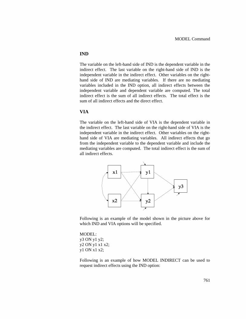
MODEL Command
761
IND
The variable on the left-hand side of IND is the dependent variable in the
indirect effect. The last variable on the right-hand side of IND is the
independent variable in the indirect effect. Other variables on the right-
hand side of IND are mediating variables. If there are no mediating
variables included in the IND option, all indirect effects between the
independent variable and dependent variable are computed. The total
indirect effect is the sum of all indirect effects. The total effect is the
sum of all indirect effects and the direct effect.
VIA
The variable on the left-hand side of VIA is the dependent variable in
the indirect effect. The last variable on the right-hand side of VIA is the
independent variable in the indirect effect. Other variables on the right-
hand side of VIA are mediating variables. All indirect effects that go
from the independent variable to the dependent variable and include the
mediating variables are computed. The total indirect effect is the sum of
all indirect effects.
Following is an example of the model shown in the picture above for
which IND and VIA options will be specified.
MODEL:
y3 ON y1 y2;
y2 ON y1 x1 x2;
y1 ON x1 x2;
Following is an example of how MODEL INDIRECT can be used to
request indirect effects using the IND option:

CHAPTER 17
762
MODEL INDIRECT:
y3 IND y1 x1;
y3 IND y2 x1;
y3 IND x2;
The first IND statement requests the specific indirect effect from x1 to
y1 to y3. The second IND statement requests the specific indirect effect
from x1 to y2 to y3. The third IND statement requests all indirect effects
from x2 to y3. These include x2 to y1 to y3, x2 to y2 to y3, and x2 to y1
to y2 to y3.
Following is an example of how MODEL INDIRECT can be used to
request indirect effects using the VIA option:
MODEL INDIRECT:
y3 VIA y1 x1 ;
The VIA statement requests all indirect effects from x1 to y3 that are
mediated by y1. These include x1 to y1 to y3 and x1 to y1 to y2 to y3.
Following is an example of how MODEL INDIRECT can be used to
request total, total indirect, specific indirect, and direct effects:
MODEL INDIRECT:
y3 IND x1;
The IND statement requests all indirect effects from x1 to y3. These
include x1 to y1 to y3, x1 to y2 to y3, and x1 to y1 to y2 to y3, the total
effect, and the total indirect effect.
COUNTERFACTUALLY-DEFINED CAUSAL
EFFECTS
Counterfactually-defined total natural indirect effects (TNIE), pure
natural direct effects (PNDE), and total effects are available for
continuous, binary, and ordered categorical (ordinal) mediators and
continuous, binary, ordered categorical (ordinal) and count outcomes.
Continuous mediators and outcomes can be observed continuous
variables or continuous latent variables. The exposure variable can be
binary or continuous. Counterfactually-defined total natural indirect

MODEL Command
763
effects, pure natural direct effects, and total effects are available for a
single mediator. These effects are obtained using the IND and MOD
options. The IND option is used to specify a specific indirect effect
when there is no moderation. The MOD option is used to specify a
specific indirect effect when there is moderation.
IND
The IND option is used to specify a specific indirect effect when there is
no moderation. Following is an example of how to specify the IND
option with a binary exposure variable:
MODEL INDIRECT:
y IND m x;
where y is the outcome, m is the mediator, and x is a binary exposure
variable. The outcome and mediator can be continuous latent variables.
When the exposure variable is continuous, two values must be given in
parentheses following the exposure variable. The causal effects are
computed comparing these two values. The default is one for the first
value and zero for the second value corresponding to a binary exposure
variable such as comparing a treatment group to a control group.
Following is an example of how to specify the IND option with a
continuous exposure variable:
MODEL INDIRECT:
y IND m x (1 -1);
where y is the outcome, m is the mediator, and x is the continuous
exposure variable. The two values in parentheses following x are the
values used to compute the causal effects, in this case, comparing 1 to -
1, which represents an increase in x from -1 to 1. The outcome,
mediator, and the exposure variable can be continuous latent variables.
MOD
The MOD option is used to specify a specific indirect effect when there
is moderation. The MOD option can have three, four, or five arguments
on the right-hand side of MOD. If the model contains continuous
control variables, they should be centered for more meaningful results.
CHAPTER 17
764
If they are centered, indirect and direct effects are evaluated using their
means. If they are not centered, indirect and direct effects are evaluated
at the value zero.
The MOD option has three arguments when there is an interaction
between the exposure variable and the mediator. Following is an
example of how to specify the MOD option with three arguments:
MODEL INDIRECT:
y MOD m mx x;
where y is the outcome, m is the mediator, mx is the interaction between
m and x, and x is a binary exposure variable. The variables must be
given in this order. The outcome can be a continuous latent variable.
When a model contains a moderator variable in addition to an exposure
and a mediator variable, a moderator plot is available showing the
effects and their confidence intervals as a function of different values of
the moderator variable. The MOD option with a moderator can have
four or five arguments. The moderation plots are obtained by specifying
TYPE=PLOT2 or TYPE=PLOT3 in the PLOT command.
The MOD option followed by four arguments has two specifications.
The moderator can interact with either the mediator or the exposure
variable. Following is an example of how to specify the MOD option
with four arguments when the moderator interacts with the mediator:
MODEL INDIRECT:
y MOD m z (-1 1 0.1) mz x;
where y is the outcome, m is the mediator, z is the moderator, mz is the
interaction between m and z, and x is a binary exposure variable. The
variables must be given in this order. The numbers in parentheses
following z are the lower limit, upper limit, and the increment to be used
in evaluating and plotting the direct and indirect effects. The outcome
can be a continuous latent variable.
Following is an example of how to specify the MOD option with four
arguments when the moderator interacts with the mediator and the
exposure variable is continuous:
MODEL Command
765
MODEL INDIRECT:
y MOD m z (-1 1 0.1) mz x (1 -1);
where y is the outcome, m is the mediator, z is the moderator, mz is the
interaction between m and z, and x is a continuous exposure variable.
The variables must be given in this order. The numbers in parentheses
following z are the lower limit, upper limit, and the increment to be used
in evaluating and plotting the direct and indirect effects. The two values
in parentheses following x are the values used to compute the causal
effects, in this case, comparing 1 to -1, which represents an increase in x
from -1 to 1. The outcome and the exposure variable can be continuous
latent variables.
Following is an example of how to specify the MOD option with four
arguments when the moderator interacts with the binary exposure
variable:
MODEL INDIRECT:
y MOD m z (-1 1 0.1) xz x;
where y is the outcome, m is the mediator, z is the moderator, xz is the
interaction between x and z, and x is a binary exposure variable. The
variables must be given in this order. The numbers in parentheses
following z are the lower limit, upper limit, and the increment to be used
in evaluating and plotting the direct and indirect effects. The mediator
and outcome can be continuous latent variables.
The MOD option has five arguments when a moderator interacts with
both the mediator and the exposure variable. Following is an example of
how to specify the MOD option with five arguments:
MODEL INDIRECT:
y MOD m z (-1 1 0.1) mz xz x;
where y is the outcome, m is the mediator, z is the moderator, mz is the
interaction between m and z, xz is the interaction between x and z, and x
is a binary exposure variable. The variables must be given in this order.
The numbers in parentheses following z are the lower limit, upper limit,
and the increment to be used in evaluating and plotting the direct and
indirect effects. The outcome can be a continuous latent variable.
CHAPTER 17
766
If the special direct effect referred to as the controlled direct effect is
wanted, a value of the mediator must be given in parentheses following
the mediator variable. Following is an example of how to specify the
IND option with a binary exposure variable:
MODEL INDIRECT:
y IND m (2) x;
where y is the outcome, m is the mediator, and x is the binary exposure
variable. The value in parentheses following m is used to compute the
controlled direct effect.
THE MODEL CONSTRAINT COMMAND
The MODEL CONSTRAINT command is used to define linear and non-
linear constraints on the parameters in the model and to create new
parameters using the parameters in the model. These constraints can be
implicit or explicit. The default setting for the INFORMATION option
of the ANALYSIS command for MODEL CONSTRAINT is
OBSERVED. The MODEL CONSTRAINT command is not available
for TYPE=EFA.
LABELING THE PARAMETERS AND
SELECTING VARIABLES
The MODEL CONSTRAINT command specifies parameter constraints
using labels defined for parameters in the MODEL command, labels
defined for parameters not in the MODEL command using the NEW
option of the MODEL CONSTRAINT command, and names of observed
variables that are identified using the CONSTRAINT option of the
VARIABLE command. See Labeling Parameters to see how parameters
are labeled using the MODEL command.
NEW
The NEW option is used to assign labels and starting values to
parameters not in the analysis model. These parameters are used to
constrain the parameters in the analysis model. The default starting
value for these parameters is 0.5. Following is an example of how the
NEW option is specified:
MODEL Command
767
MODEL:
[y1-y3] (p1-p3);
MODEL CONSTRAINT:
NEW (c*.6);
p2 = p1 + c;
p3 = p1 + 2*c;
where c is a parameter that constrains the means to change linearly
across the three variables. The value .6 following the asterisk (*)
specifies that the value .6 will be used as a starting value for model
estimation. If the analysis is a Monte Carlo simulation study, the value
will also be used as a coverage value.
CONSTRAINT
The CONSTRAINT option of the VARIABLE command is used to
identify the variables that can be used in the MODEL CONSTRAINT
command. These can be not only variables used in the MODEL
command but also other variables. All variables on the CONSTRAINT
list are treated as continuous variables in the analysis. Only variables
used by the following options cannot be included: GROUPING,
PATTERN, COHORT, COPATTERN, CLUSTER, STRATIFICATION,
and AUXILIARY. Variables that are part of these options can be used
in DEFINE to create new variables that can be used in the
CONSTRAINT statement. The CONSTRAINT option is not available
for TYPE=RANDOM, TYPE=TWOLEVEL, TYPE=THREELEVEL,
TYPE=CROSSCLASSIFIED, TYPE=COMPLEX, and for estimators
other than ML, MLR, and MLF. The CONSTRAINT option is specified
as follows:
CONSTRAINT = y1 u1;
where y1 and u1 are variables that can be used in the MODEL
CONSTRAINT command.
DEFINING LINEAR AND NON-LINEAR
CONSTRAINTS
Linear and non-linear constraints can be defined using the equal sign (=),
the greater than sign (>), the less than sign (<), and all arithmetic

CHAPTER 17
768
operators and functions that are available in the DEFINE command with
the exception of the absolute value function.
In the MODEL CONSTRAINT command, labels from the MODEL
command and the NEW option of the MODEL CONSTRAINT
command can be used on both the left-hand and right-hand sides of one
or more parameter constraint statements. Variables listed on the
CONSTRAINT option of the VARIABLE command can appear on the
right-hand side of one or more parameter constraint statements.
Following is an example of how to define an explicit constraint:
MODEL:
[y1-y3] (p1-p3);
MODEL CONSTRAINT:
p1 = p2**2 + p3**2;
where the parameter p1 is constrained to be equal to the sum of the
squares of the p2 and p3 parameters.
Following is an example of how to define an implicit constraint where a
function of parameters is constrained to be zero:
MODEL:
[y1-y5] (m1-m5);
MODEL CONSTRAINT:
0 = - m4 + m1*m3 - m2;
0 = exp(m3) - 1 - m2;
0 = m4 - m5;
Following is an example of how to define an implicit constraint where a
parameter appears in a set of parameter constraints:
MODEL:
[y1-y4] (p1-p4);
MODEL CONSTRAINT:
p1 = p2**2 + p3**2;
p2 = p4;

MODEL Command
769
DO
The DO option provides a do loop and a double do loop to facilitate
specifying a set of new parameters that are a function of the parameters
of the model. Following is an example of how to specify a do loop:
MODEL:
y1 ON x1 (p1);
y1 ON x2 (p2);
y1 ON x3 (p3);
y2 ON x1 (q1);
y2 ON x2 (q2);
y2 ON x3 (q3);
MODEL CONSTRAINT:
NEW (ratio1-ratio3);
DO (1, 3) ratio# = p#/q#;
where the numbers in parentheses give the range of values for the do
loop. The number sign (#) is replaced by these values during the
execution of the do loop. Following are the new parameters that are
created based on the DO option specified above:
ratio1 = p1/q1;
ratio2 = p2/q2;
ratio3 = p2/q3;
The DO option can also be used to place constraints on a set of
parameters. Following is an example of how to use a do loop to
constrain the residual variances of y1 through y4 to be greater than zero:
MODEL:
f BY y1-y4;
y1-y4 (p1-p4);
MODEL CONSTRAINT:
DO (1, 4) p# > 0;
where the numbers in parentheses give the range of values for the do
loop. The number sign (#) is replaced by these values during the

CHAPTER 17
770
execution of the do loop. Following are the constraints that are placed
on the model parameters based on the DO option specified above:
p1 > 0;
p2 > 0;
p3 > 0;
p4 > 0;
Following is an example of how to specify a double do loop:
MODEL:
y1 ON x1 (p1);
y2 ON x2 (p2);
y3 ON x3 (q3);
y4 ON x4 (q4);
MODEL CONSTRAINT:
DO ($,1,2) DO (%,3,4) p$ = q%;
where the numbers in parentheses give the range of values the double do
loop will use. The numbers replace the symbol preceding them.
Following are the constraints that are placed on the model parameters
based on the DO option specified above:
p1 = q3;
p1 = q4;
p2 = q3;
p2 = q4;
PLOT
The PLOT option is used to name the variables that will be plotted on
the y-axis in the plots created using the LOOP option. Following is an
example of how to specify the PLOT option:
PLOT (ind1 ind2);
where ind1 and ind2 are the variables that will be plotted on the y-axis in
the plots created using the LOOP option.
MODEL Command
771
LOOP
The LOOP option is used in conjunction with the PLOT option to create
plots of variables. For example, it is useful for plotting indirect effects
with moderation and mediation (Preacher, Rucker, & Hayes, 2007),
cross-level interactions in multilevel regression (Bauer & Curran, 2005),
and sensitivity graphs for causal effect mediation modeling (Imai, Keele,
& Tingley, 2010a; Muthén, 2011; Muthén, Muthén, & Asparouhov,
2016). Following is an example of how to specify the LOOP option:
LOOP (mod, -1, 1, 0.01);
where mod is a variable that will be used on the x-axis, the numbers -1
and 1 are the lower and upper values of mod, and 0.01 is the incremental
value of mod to use in the computations. When mod appears in a
MODEL CONSTRAINT statement involving a new parameter, that
statement is evaluated for each value of mod specified by the LOOP
option. For example, the first value of mod is -1; the second value of
mod is -1 plus 0.01 or -0.99; the third value of mod is -0.99 plus 0.01 or -
0.98; the last value of mod is 1. Plots are created with mod on the x-axis
and the names in the PLOT option on the y-axis.
Following is an example of how to use the PLOT and LOOP options
with the MODEL and MODEL CONSTRAINT commands:
MODEL:
y ON x (p1);
MODEL CONSTRAINT:
PLOT (ypred);
LOOP (age, 10, 50, 1);
ypred = p1*age;
Using TYPE=PLOT2 in the PLOT command, the plot of ypred and age
can be viewed by choosing Loop plots from the Plot menu of the Mplus
Editor. The plot presents the computed values along with a 95%
confidence interval. For frequentist estimation, the default confidence
interval uses plus and minus 1.96 times the standard error. The
CINTERVAL option of the OUTPUT command can be used in
conjunction with the BOOTSTRAP option of the ANALYSIS command
to obtain bootstapped or bias-corrected bootstrap confidence intervals.
CHAPTER 17
772
For Bayesian estimation, the default is credibility intervals of the
posterior distribution with equal tail percentages. The CINTERVAL
option of the OUTPUT command can be used to obtain credibility
intervals of the posterior distribution that give the highest posterior
density.
THE MODEL TEST COMMAND
The MODEL TEST command is used to test restrictions on the
parameters in the MODEL and MODEL CONSTRAINT commands
using the Wald chi-square test. These restrictions are defined using
labels from the MODEL command and new parameters from the NEW
option of the MODEL CONSTRAINT command. See Labeling
Parameters to see how parameters are labeled using the MODEL
command. See the NEW option to see how new parameters are named
using this option. Variables listed on the CONSTRAINT statement of
the VARIABLE command cannot be used in MODEL TEST. Model
restrictions can be defined using the equal sign (=) and all arithmetic
operators and functions that are available in the DEFINE command with
the exception of the absolute value function.
Following is an example of how to test restrictions on the parameters in
the MODEL command using MODEL TEST:
MODEL:
y ON x1 (p1)
x2 (p2)
x3 (p3);
MODEL TEST:
0 = p2 – p1;
0 = p3 – p1;
where in the MODEL command p1, p2, and p3 represent the regression
coefficients for x1, x2, and x3, respectively. In the MODEL TEST
command, a joint test of the equality of the three regression coefficients
is carried out using the Wald test with two degrees of freedom. Note
that having 0 = p3 - p2 in MODEL TEST is redundant and incorrect.

MODEL Command
773
Following is an example of how to test a restriction on the parameters in
the MODEL CONSTRAINT command using MODEL TEST:
MODEL:
y ON m1 (b1);
y ON m2 (b2);
m1 ON x1 (a1);
m2 ON x2 (a2);
MODEL CONSTRAINT:
NEW (ind1 ind2);
ind1 = a1*b1;
ind2 = a2*b2;
MODEL TEST:
0 = ind1 – ind2;
where in the MODEL command b1 and b2 represent the regression
coefficients for m1 and m2 and a1 and a2 represent the regression
coefficients for x1 and x2. In the MODEL CONSTRAINT command,
two new parameters are defined. Ind1 is the indirect effect from x1 to y
via m1. Ind2 is the indirect effect from x2 to y via m2. In the MODEL
TEST command, a test of the equality of the two indirect effects is
carried out using the Wald test with one degree of freedom.
DO
The DO option provides a do loop and a double do loop to facilitate
specifying a set of tests involving model parameters that will be jointly
tested using the Wald test. Following is an example of how to specify a
do loop:
MODEL:
y1 ON x1 (p1);
y1 ON x2 (p2);
y1 ON x3 (p3);
y2 ON x1 (q1);
y2 ON x2 (q2);
y2 ON x3 (q3);
MODEL TEST:
DO (1, 3) 0 = p# - q#;
CHAPTER 17
774
where the numbers in parentheses give the range of values for the do
loop. The number sign (#) is replaced by these values during the
execution of the do loop. Following is the set of tests involving model
parameters that will be jointly tested using the Wald test based on the
DO option specified above:
0 = p1 – q1;
0 = p2 – q2;
0 = p3 – q3;
Following is an example of how to specify a double do loop:
MODEL:
y1 ON x1 (p1);
y1 ON x2 (p2);
y1 ON x3 (p3);
y2 ON x1 (q1);
y2 ON x2 (q2);
y2 ON x3 (q3);
MODEL TEST:
DO (#,1,3) DO ($,1,3) 0 = p# - q$;
where the numbers in parentheses give the range of values the double do
loop will use. The numbers replace the symbol preceding them.
Following is the set of tests involving model parameters that will be
jointly tested using the Wald test based on the DO option specified
above:
0 = p1 – q1;
0 = p1 – q2;
0 = p1 – q3;
0 = p2 – q1;
0 = p2 – q2;
0 = p2 – q3;
0 = p3 – q1;
0 = p3 – q2;
0 = p3 – q3;
MODEL Command
775
THE MODEL PRIORS COMMAND
The MODEL PRIORS command is used with ESTIMATOR=BAYES to
specify the prior distribution for each parameter. The default is to use
diffuse (non-informative) priors. Following is a table that shows the
distributions available and the default priors for different types of
parameters:
Type of Parameter Distributions Available Default Priors
Observed continuous dependent variable means/intercepts (nu)
normal normal (0, infinity)
Observed continuous dependent variable variances/residual variances (theta)
inverse Gamma inverse Gamma (-1, 0)
Observed categorical dependent variable thresholds (tau)
normal uniform
normal (0, infinity)
Factor loadings (lambda) normal normal (0, infinity)* normal (0, 5)**
Regression coefficients (beta) normal normal (0, infinity)* normal (0, 5)**
Continuous latent variable means/intercepts (alpha)
normal normal (0, infinity)
Continuous latent variable variances/residual variances (psi)
One latent variable inverse Gamma Gamma uniform lognormal normal More than one latent variable inverse Wishart
inverse Gamma (-1, 0) inverse Wishart (0, -p-1)***
Categorical latent variable parameters (varies)
Dirichlet Dirichlet (10, 10)
* Continuous variables
** Categorical variables
*** Not available for GIBBS(RW)
For the normal distribution default, infinity is ten to the power of ten.
For the inverse Gamma default, the settings imply a uniform prior
ranging from minus infinity to plus infinity. For the inverse Wishart
default, p is the dimension of the multivariate block of latent variables.

CHAPTER 17
776
For the Dirichlet default, the first number gives the number of
observations to add to the class referred to and the second number gives
the number of observations to add to the last class. For a discussion of
priors, see Gelman et al. (2004), Browne and Draper (2006), and Gelman
(2006).
ASSIGNING PRIORS TO PARAMETERS
Priors are assigned to the parameters using the tilde (~) symbol, which
means distributed as, using the following distribution settings:
Normal – N
Lognormal – LN
Uniform – U
Inverse Gamma – IG
Gamma – G
Inverse Wishart – IW
Dirichlet – D
Each setting has two numbers in parentheses following the setting. For
the normal and lognormal distributions, the first number is the mean and
the second number is the variance. For the uniform distribution, the first
number is the lower limit and the second number is upper limit. For the
inverse Gamma distribution, the first number is the shape parameter and
the second number is the scale parameter. For the Gamma distribution,
the first number is the shape parameter and the second number is the
inverse scale parameter. For the inverse Wishart distribution, the first
number is used to form a covariance matrix and the second number is the
degrees of freedom. For the Dirichlet distribution, the first number gives
the number of observations to add to the class referred to and the second
number gives the number of observations to add to the last class. For a
technical description of the implementation of priors, see Asparouhov
and Muthén (2010b).
In the MODEL PRIORS command, labels from the MODEL command
are used to represent parameters for which prior distributions are
specified. See Labeling Parameters to see how parameters are labeled
using the MODEL command. Following is an example of how to assign
priors to the factor loading parameters:
MODEL Command
777
MODEL:
f BY y1-y10* (p1-p10);
f@1;
MODEL PRIORS:
p1-p10 ~ N (1, 0.5);
where parameters p1 through p10 have normal priors with mean one and
variance 0.5.
COVARIANCE
The COVARIANCE option is used to assign a prior to the covariance
between two parameters. Only normal priors are available. Covariance
priors can be assigned to only factor loadings, regression coefficients,
intercepts, and thresholds for binary variables. Following is an example
of how to specify the COVARIANCE option:
MODEL:
y ON x1 (p1)
x2 (p2);
MODEL PRIORS:
p1 ~ N (10, 4);
p2 ~ N (6, 1);
COVARIANCE (p1, p2) = 0.5;
where the bivariate prior distribution of p1 and p2 has a covariance of
0.5 which corresponds to a correlation of 0.25 computed as 0.5 / (sqrt (4)
* sqrt (1)).
DO
The DO option provides a do loop and a double do loop to facilitate
specifying the same prior for a set of parameters. With MODEL
PRIORS it can be used with the DIFFERENCE option to assign priors to
differences among a set of parameters. Following is an example of how
to specify a do loop:

CHAPTER 17
778
MODEL:
f1 BY y1-y20;
f2 BY y1-y10
y11-y20 (s1-s10);
MODEL PRIORS:
DO (1,10) s# ~ N (0,0.1);
where the numbers in parentheses give the range of values for the do
loop. The number sign (#) is replaced by these values during the
execution of the do loop. Following are the statements that are
generated based on the DO option specified above:
s1 ~ N (0,0.1);
s2 ~ N (0,0.1);
s3 ~ N (0,0.1);
s4 ~ N (0,0.1);
s5 ~ N (0,0.1);
s6 ~ N (0,0.1);
s7 ~ N (0,0.1);
s8 ~ N (0,0.1);
s9 ~ N (0,0.1);
s10 ~ N (0,0.1);
Following is an example of how to specify a double do loop for a
multiple group model:
MODEL:
f1 BY y1-y20;
f2 BY y1-y15
y16-y20 (s#_1-s#_5);
MODEL PRIORS:
DO (#,1,2) DO ($,1,5) s#_$ ~ N (0,0.1);
where the numbers in parentheses give the range of values the double do
loop will use. The numbers replace the symbol preceding them. In this
example, the first do loop refers to the two groups. Following are the
statements that are generated based on the DO option specified above:

MODEL Command
779
s1_1 ~ N (0,0.01);
s1_2 ~ N (0,0.01);
s1_3 ~ N (0,0.01);
s1_4 ~ N (0,0.01);
s1_5 ~ N (0,0.01);
s2_1 ~ N (0,0.01);
s2_2 ~ N (0,0.01);
s2_3 ~ N (0,0.01);
s2_4 ~ N (0,0.01);
s2_5 ~ N (0,0.01);
DIFFERENCE
The DIFFERENCE option is used to assign priors to the difference
between two parameters. Only normal priors are available. Difference
priors can be assigned to only factor loadings, regression coefficients,
intercepts, and thresholds for binary variables. Following is an example
of how to specify the DIFFERENCE option:
MODEL:
y ON x1 (p1)
x2 (p2);
MODEL PRIORS:
DIFFERENCE (p1, p2) ~ N (0, 0.01);
where the difference between p1 and p2 has a normal prior with mean
zero and variance 0.01.
The DO option provides a do loop to facilitate specifying the same
expression for a set of parameters. The DO and DIFFERENCE options
can be used together to simplify the assignment of priors to a large set of
difference parameters for models with multiple groups and multiple time
points. In Bayesian estimation, multiple group analysis is obtained using
TYPE=MIXTURE and the KNOWNCLASS option. Following is an
example of how to use the DO and DIFFERENCE options to assign
priors to differences across groups among a set of parameters:
CHAPTER 17
780
MODEL:
%OVERALL%
f BY y1-y5;
%c#1%
f BY y2-y5 (p12-p15);
%c#2%
f BY y2-y5 (p22-p25);
%c#3%
f BY y2-y5 (p32-p35);
MODEL PRIORS:
DO (2, 5) DIFFERENCE (p1#-p3#) ~ N (0, 0.01);
where the numbers in parentheses give the range of values for the do
loop. The number sign (#) is replaced by these values during the
execution of the do loop. Following are the differences that were
assigned normal priors with mean zero and variance 0.01:
p12 - p22
p12 - p32
p22 - p32
p13 - p23
p13 - p33
p23 - p33
p14 - p24
p14 - p34
p24 - p34
p15 - p25
p15 - p35
p25 - p35
MODEL COMMAND VARIATIONS
The MODEL command is used to describe the analysis model using the
options described in the previous sections. This section discusses
variations of the MODEL command for use with multiple group models,
mixture models, multilevel models, and models for generating data for
Monte Carlo simulations studies.

MODEL Command
781
MODEL:
The MODEL command is used to describe the analysis model for a
single group analysis and the overall analysis model for multiple group
analysis.
MODEL label:
MODEL followed by a label is used to describe the group-specific
analysis models in multiple group analysis and the analysis model for
each categorical latent variable in mixture modeling when there are more
than one categorical latent variable in the analysis.
In multiple group analysis, MODEL followed by a label is used to
describe differences between the overall analysis model described in the
MODEL command and the analysis model for each group. Labels are
defined using the GROUPING option of the VARIABLE command for
raw data in a single file, by the FILE option of the DATA command for
raw data in separate files, and by the program for summary data.
MODEL followed by a label is used in conjunction with the
%WITHIN% and %BETWEEN% specifications in multiple group
multilevel analysis.
In mixture modeling, MODEL followed by a label is used to describe the
analysis model for each categorical latent variable when there are more
than one categorical latent variable in the analysis and for combinations
of categorical latent variables when there are more than two categorical
latent variables in the analysis. Labels are defined by using the names of
the categorical latent variables.
When there are more than one categorical latent variable in the model,
the class-specific parts of the model for each categorical latent variable
must be specified within a MODEL command for that categorical latent
variable. The %OVERALL% specification is not included in the
MODEL commands for each categorical latent variable. Following is an
example of how to specify the MODEL command when there are more
than one categorical latent variable in the model:

CHAPTER 17
782
MODEL c1:
%c1#1%
%c1#2%
where the class-specific parts of the model for c1 is specified after
MODEL c1.
When there are more than two categorical latent variables in the model,
MODEL commands for pairs of categorical latent variables are allowed.
These are used to specify parameters that are specific to the
combinations of classes for those two categorical latent variables.
Categorical latent variables can be combined in sets involving all but one
categorical latent variable. For example, with three categorical latent
variables c1, c2, and c3, combinations of up to two categorical latent
variables are allowed. Following is an example of how this is specified:
MODEL c1.c2:
%c1#1.c2#1%
where %c1#1.c2#1% refers to a combination of class 1 for c1 and class 1
for c2.
MODEL:
%OVERALL%
%class label%
The MODEL command used in conjunction with %OVERALL% and
%class label% is used to describe the overall and class-specific models
for mixture models. Statements following %OVERALL% refer to the
model common to all latent classes. Statements following %class
label% refer to class-specific model statements.
Class labels are created by adding to the name of the categorical latent
variable a number sign (#) followed by the class number. For example,
if c is a categorical latent variable with two latent classes, the class
labels are c#1 and c#2.
MODEL Command
783
MODEL:
%WITHIN%
%BETWEEN%
%BETWEEN label%
The MODEL command used in conjunction with %WITHIN%,
%BETWEEN%, and %BETWEEN label% is used to describe the
individual-level and cluster-level models for multilevel modeling. For
TYPE=TWOLEVEL, the statements following %WITHIN% describe
the individual-level model and the statements following %BETWEEN%
describe the cluster-level model. With multilevel mixture models, the
%OVERALL% and %class label% specifications are used with the
%WITHIN% and %BETWEEN% specifications to describe the mixture
part of the model.
For TYPE=THREELEVEL and TYPE=CROSSCLASSIFIED, the
statements following %WITHIN% describe the individual-level model
and the statements following %BETWEEN label% describe the cluster-
level model. The label is a cluster variable from the CLUSTER option.
THE MODEL POPULATION COMMAND
The MODEL POPULATION command is used to provide the
population parameter values to be used in data generation using the
options of the MODEL command described earlier. The MODEL
POPULATION command has variations for use with multiple group
models, mixture models, and multilevel models. These are described
below.
In the MODEL POPULATION command, each parameter in the model
must be specified followed by the @ symbol or the asterisk (*) and the
population parameter value. Any model parameter not specified will
have the value of zero as the population parameter value.
Parameter estimates can be saved from a real data analysis using the
ESTIMATES option of the SAVEDATA command and used in a
subsequent Monte Carlo analysis as population parameter values. This
is done by using the POPULATION option of the MONTECARLO
command.

CHAPTER 17
784
MODEL POPULATION:
The MODEL POPULATION command is used to provide the
population parameter values to be used in data generation for single
group analysis and the overall analysis model for multiple group
analysis.
MODEL POPULATION-label:
MODEL POPULATION followed by a dash and a label is used to
provide parameter values to be used in the generation of data for the
group-specific analysis models in multiple group analysis and the
analysis model for each categorical latent variable in mixture modeling
when there are more than one categorical latent variable in the analysis.
In multiple group analysis, the label following the dash refers to the
group. The first group is referred to by g1, the second group by g2, and
so on. In mixture modeling, the label following the dash is the name of
each categorical latent variable when there are more than one categorical
latent variables in the generation of the data.
In addition, the NGROUPS option of the MONTECARLO command is
used for the generation of data for multiple group Monte Carlo
simulation studies.
MODEL POPULATION:
%OVERALL%
%class label%
MODEL POPULATION used in conjunction with %OVERALL% and
%class label% is used to provide the population parameter values to be
used in the generation of data for mixture models. Statements following
%OVERALL% refer to the model common to all latent classes.
Statements following %class label% refer to class-specific model
statements. In addition, the GENCLASSES option of the
MONTECARLO command is used for the generation of data for mixture
models.
The statements in the overall part of the model include information
about the means, variances, and covariances of the background variables
MODEL Command
785
and the specification of the overall model including information about
parameters that do not vary across the classes. The class-specific parts
of the model describe the parameters that vary across classes.
MODEL POPULATION:
%WITHIN%
%BETWEEN%
%BETWEEN label%
MODEL POPULATION used in conjunction with %WITHIN%,
%BETWEEN%, and %BETWEEN label% is used to provide the
population parameter values to be used in the generation of clustered
data. For TYPE=TWOLEVEL, %WITHIN% is used to provide
population parameter values for the individual-level model parameters.
%BETWEEN% is used to provide population parameter values for the
cluster-level model parameters. With multilevel mixture models, the
%OVERALL% and %class label% specifications are used with the
%WITHIN% and %BETWEEN% specifications to provide the
population parameter values to be used in the generation of data for
mixture models.
For TYPE=THREELEVEL and TYPE=CROSSCLASSIFIED,
%WITHIN% is used to provide population parameter values for the
individual-level model parameters. %BETWEEN label% is used to
provide population parameter values for the cluster-level model
parameters. For TYPE=THREELEVEL, the labels level2 and level3 are
used to provide the level 2 and level 3 population parameter values. For
TYPE=CROSSCLASSIFIED, the labels level2a and level2b are used to
describe the level 2a and level 2b population parameter values.
In addition, the NCSIZES, CSIZES, BETWEEN, and WITHIN options
of the MONTECARLO command are used for the generation of
clustered data.
THE MODEL COVERAGE COMMAND
In Monte Carlo simulation studies, the MODEL command describes not
only the analysis model but also provides values for each parameter that
are used both as the population parameter values for computing coverage
and as starting values in the estimation of the model. If the MODEL

CHAPTER 17
786
COVERAGE command is used, coverage is computed using the
population parameter values specified in the MODEL COVERAGE
command, and the values specified in the MODEL command are used
only as starting values. The MODEL COVERAGE command has
special options for multiple group models, mixture models, and
multilevel models.
In MODEL COVERAGE, each parameter in the model must be
specified followed by the @ symbol or the asterisk (*) and the
population parameter value. Any model parameter not specified will
have the value of zero as the population parameter value.
Parameter estimates can be saved from a real data analysis using the
ESTIMATES option of the SAVEDATA command and used in a
subsequent Monte Carlo analysis as population parameter values. This
is done by using the COVERAGE option of the MONTECARLO
command.
MODEL COVERAGE:
The MODEL COVERAGE command is used to provide the population
parameter values to be used for computing coverage for single group
analysis and the overall analysis model for multiple group analysis.
MODEL COVERAGE-label:
MODEL COVERAGE followed by a dash and a label is used in multiple
group analysis to provide group-specific parameter values to be used in
computing coverage. The label following the dash refers to the group.
The first group is referred to by g1, the second group by g2, and so on.
In mixture modeling, the label following the dash is the name of each
categorical latent variable when there are more than one categorical
latent variable.
MODEL COVERAGE:
%OVERALL%
%class label%
MODEL COVERAGE used in conjunction with %OVERALL% and
%class label% is used to provide the population parameter values to be

MODEL Command
787
used in computing coverage. Statements following %OVERALL% refer
to the model common to all latent classes. Statements following %class
label% refer to class-specific model statements.
Class labels are created by adding to the name of the categorical latent
variable a number sign (#) followed by the class number. For example,
if c1 is a categorical latent variable with two latent classes, the class
labels are c1#1 and c1#2.
The statements in the overall part of the model include information
about the means, variances, and covariances of the background variables
and the specification of the overall model including information about
latent class parameters that do not vary across the classes. The class-
specific parts of the model describe the latent class parameters that do
vary across classes.
MODEL COVERAGE:
%WITHIN%
%BETWEEN%
%BETWEEN label%
MODEL COVERAGE used in conjunction with %WITHIN% and
%BETWEEN% is used to provide the population parameter values to be
used in computing coverage. For TYPE=TWOLEVEL, %WITHIN% is
used to provide the population parameter values for the individual-level
model parameters. %BETWEEN% is used to provide the population
parameter values for the cluster-level model parameters.
For TYPE=THREELEVEL and TYPE=CROSSCLASSIFIED,
%WITHIN% is used to provide population parameter values for the
individual-level model parameters. %BETWEEN label% is used to
provide population parameter values for the cluster-level model
parameters. For TYPE=THREELEVEL, the labels level2 and level3 are
used to provide the level 2 and level 3 population parameter values. For
TYPE=CROSSCLASSIFIED, the labels level2a and level2b are used to
describe the level 2a and level 2b population parameter values.

CHAPTER 17
788
THE MODEL MISSING COMMAND
The MODEL MISSING command is used to provide information about
the population parameter values for the missing data model to be used in
the generation of data. The MODEL MISSING command has special
options for multiple group models and for mixture models. The
MISSING option of the MONTECARLO command is required for
MODEL MISSING.
Each parameter in the model must be specified followed by the @
symbol or the asterisk (*) and the population parameter value. Any
model parameter not specified will have the value of zero as the
population parameter value.
Information about each variable listed in the MISSING statement of the
MONTECARLO command must be included as part of the MODEL
MISSING command. These variables must be dependent variables in
the MODEL command. The probability of having missing data or not on
these dependent variables is described by logistic regressions in the
MODEL MISSING command. In the MODEL MISSING command, the
missing data indicators use the same names as the dependent variables in
the MODEL command. For each dependent variable, the intercept and
slopes for all covariates must be specified for the logistic regression.
The covariates in these logistic regressions can be both independent and
dependent variables in the MODEL command. When a dependent
variable in the MODEL command is used as a dependent variable in the
logistic regression, it is a missing value indicator. When it is used as a
covariate in the logistic regression, it is the original variable in the
MODEL command. In the following example, in the first ON statement
y1 is a missing value indicator variable. In the second ON statement, y1
is treated as the original variable.
MODEL MISSING:
y1 ON x;
y2 ON y1 x;
A dependent variable that is censored, categorical, or count is treated as
a continuous covariate in the logistic regressions.

MODEL Command
789
MODEL MISSING:
The MODEL MISSING command is used to provide information about
the population parameter values for the missing data model to be used in
the generation of data for single group analysis and the overall analysis
model for multiple group analysis.
MODEL MISSING-label: MODEL MISSING followed by a dash and a label is used in multiple
group analysis to provide group-specific population parameter values for
the missing data model to be used in the generation of data. The label
following the dash refers to the group. The first group is referred to by
g1, the second group by g2, and so on.
MODEL MISSING:
%OVERALL%
%class label%
MODEL MISSING used in conjunction with %OVERALL% and %class
label% is used to provide the population parameter values for the
missing data model to be used in the generation of data for mixture
models. Statements following %OVERALL% refer to the model
common to all latent classes. Statements following %class label% refer
to class-specific model statements.
Class labels are created by adding to the name of the categorical latent
variable a number sign (#) followed by the class number. For example,
if c1 is a categorical latent variable with two latent classes, the class
labels are c1#1 and c1#2.

CHAPTER 17
790