Chapter 2

Stellar Dynamics in Galaxies

2.1 Introduction

A system of stars behaves like a fluid, but one with unusual properties. In a normalfluid two-body interactions are crucial in the dynamics, but in contrast star-star en-counters are very rare. Instead stellar dynamics is mostly governed by the interactionof individual stars with the mean gravitational field of all the other stars combined.This has profound consequences for how the dynamics of the stars within galaxies aredescribed mathematically, allowing for some considerable simplifications.

This chapter establishes some basic results relating to the motions of stars withingalaxies. The virial theorem provides a very simple relation between the total potentialand kinetic energies of stars within a galaxy, or other system of stars, that has settleddown into a steady state. The virial theorem is derived formally here. The timescale forstars to cross a system of stars, known as the crossing time, is a simple but importantmeasure of the motions of stars. The relaxation time measures how long it takes fortwo-body encounters to influence the dynamics of a galaxy, or other system of stars.An expression for the relaxation time is derived here, which is then used to show thatencounters between stars are so rare within galaxies that they have had little effectover the lifetime of the Universe.

The motions of stars within galaxies can be described by the collisionless Boltzmannequation, which allows the numbers of stars to be calculated as a function of positionand velocity in the galaxy. The equation is derived from first principles here. Similarly,the Jeans Equations relate the densities of stars to position, velocity, velocity dispersionand gravitational potential.

2.2 The Virial Theorem

2.2.1 The basic result

Before going into the main material on stellar dynamics, it is worth stating – andderiving – a basic principle known as the virial theorem. It states that for any systemof particles bound by an inverse-square force law, the time-averaged kinetic energy〈T 〉 and the time-averaged potential energy 〈U〉 satisfy

2 〈T 〉 + 〈U〉 = 0 , (2.1)

15

for a steady equilibrium state. 〈T 〉 will be a very large positive quantity and 〈U〉 avery large negative quantity. Of course, for a galaxy to hold together, the total energy〈T 〉+ 〈U〉 < 0 ; the virial theorem provides a much tighter constraint than this alone.Typically, 〈T 〉 and −〈U〉 ∼ 1050 to 1054 J for galaxies.

In practice, many systems of stars are not in a perfect final steady state and thevirial theorem does not apply exactly. Despite this, it does give important, approxi-mate results for many astronomical systems.

The virial theorem was first devised by Rudolf Clausius (1822–1888) to describemotions of particles in thermodynamics. The term virial comes from the Latin wordfor force, vis.

2.2.2 Deriving the virial theorem from first principles

To prove the virial theorem, consider a system of N stars. Let the ith star have a massmi and a position vector xi. The position vector will be measured from the centre ofmass of the system, and we shall assume that this centre of mass moves with uniformmotion. The velocity of the ith star is xi ≡ dxi/dt, where t is the time.Consider the moment of inertia I of this system of stars defined here as

I ≡N∑

i=1

mi xi.xi =

N∑

i=1

mi x2i . (2.2)

(Note that this is a different definition of moment of inertia to the moment of inertiaabout a particular axis that is used to study the rotation of bodies about an axis.)Differentiating with respect to time t,

dI

dt=

d

dt

(

∑

i

mi xi.xi

)

=∑

i

d

dt

(

mi xi.xi

)

=∑

i

mid

dt

(

xi.xi

)

assuming that the masses mi do not change

=∑

i

mi

(

xi.xi + xi.xi

)

from the product rule

= 2∑

i

mi xi.xi

Differentiating again,

d2I

dt2= 2

d

dt

∑

i

mi xi.xi = 2∑

i

d

dt

(

mi xi.xi

)

= 2∑

i

mid

dt

(

xi.xi

)

= 2∑

i

mi

(

xi.xi + xi.xi

)

= 2∑

i

mi xi.xi + 2∑

i

mi xi2 (2.3)

The kinetic energy of the ith particle is 12mixi

2. Therefore the total kinetic energy ofthe entire system of stars is

T =∑

i

12mi x

2i ∴

∑

i

mi x2i = 2T

16

Substituting this into Equation 2.3,

d2I

dt2= 4T + 2

∑

i

mi xi.xi , (2.4)

at any time t.We now need to remember that the average of any parameter y(t) over time t = 0 toτ is

〈y〉 =1

τ

∫ τ

0

y(t) dt

Consider the average value of d2I/dt2 over a time interval t = 0 to τ .

⟨

d2I

dt2

⟩

=1

τ

∫ τ

0

(

4T + 2∑

i

mi xi.xi

)

dt

=4

τ

∫ τ

0

T dt +2

τ

∫ τ

0

∑

i

mi xi.xi dt

= 4 〈T 〉 + 2∑

i

mi

τ

∫ τ

0

xi.xi dt assuming mi is constant over time

= 4 〈T 〉 + 2∑

i

mi 〈xi.xi〉 (2.5)

When the system of stars eventually reaches equilibrium, the moment of inertia Iwill be constant. So, 〈d2I/dt2〉 = 0. An alternative way of visualising this is byconsidering that I will be bounded in any physical system and d2I/dt2 will alsobe finite. Therefore the long-time average 〈d2I

dt2〉 will vanish as τ becomes large, i.e.

limτ→∞〈d2Idt2

〉 = limτ→∞( 1τ

∫ τ

0d2Idt2

dt) → 0 because d2I/dt2 remains finite.

Substituting for 〈d2I/dt2〉 = 0 into Equation 2.5,

4 〈T 〉 + 2∑

i

mi 〈xi.xi〉 = 0 .

∴ 2 〈T 〉 +∑

i

mi 〈xi.xi〉 = 0 . (2.6)

The term∑

imi 〈xi.xi〉 is related to the gravitational potential. We next need to showhow.

Newton’s Second Law of Motion gives for the ith star,

mi xi =∑

jj 6=i

Fij

where Fij is the force exerted on the ith star by the jth star. Using the law of universalgravitation,

mi xi =∑

jj 6=i

− Gmimj

|xi − xj|3(xi − xj) .

Taking the scalar product (dot product) with xi,

mi xi.xi =(

∑

jj 6=i

− Gmimj

|xi − xj|3(xi − xj)

)

.xi

17

Summing over all i,

∑

i

mixi.xi = −∑

i

∑

jj 6=i

Gmimj

|xi − xj|3(xi−xj).xi = −

∑

i,ji6=j

Gmimj

|xi − xj|3(xi−xj).xi

(2.7)Switching i and j, we have

∑

j

mj xj.xj = −∑

j,ii6=j

Gmj mi

|xj − xi|3(xj − xi).xj (2.8)

Adding Equations 2.7 and 2.8,

∑

i

mixi.xi+∑

j

mjxj.xj = −∑

i,ji6=j

Gmimj

|xi − xj|3(xi−xj).xi −

∑

i,ji6=j

Gmj mi

|xj − xi|3(xj−xi).xj

∴ 2∑

i

mi xi.xi = −∑

i,ji6=j

Gmimj

|xi − xj|3(

(xi − xj).xi + (xj − xi).xj

)

But

(xi − xj).xi + (xj − xi).xj = (xi − xj).xi − (xi − xj).xj

= (xi − xj).(xi − xj) (factorising)

= |xi − xj|2

∴ 2∑

i

mi xi.xi = −∑

i,ji6=j

Gmimj

|xi − xj|3|xi − xj|2

∴∑

i

mi xi.xi = − 1

2

∑

i,ji6=j

Gmimj

|xi − xj|(2.9)

We now need to find the total potential energy of the system.The gravitational potential at star i due to star j is

Φi j = − Gmj

|xi − xj|

Therefore the gravitational potential at star i due to all other stars is

Φi =∑

jj 6=i

Φi j =∑

jj 6=i

− Gmj

|xi − xj|

Therefore the gravitational potential energy of star i due to all the other stars is

Ui = mi Φi = − mi

∑

jj 6=i

Gmj

|xi − xj|

18

The total potential energy of the system is therefore

U =∑

i

Ui =1

2

∑

i

−mi

∑

jj 6=i

Gmj

|xi − xj|

The factor 12

ensures that we only count each pair of stars once (otherwise we wouldcount each pair twice and would get a result twice as large as we should). Therefore,

U = − 1

2

∑

i,ji6=j

Gmimj

|xi − xj|

Substituting for the total potential energy into Equation 2.9,

∑

i

mi xi.xi = U

Equation 2.6 uses time-averaged quantities. So, averaging over time t = 0 to τ ,

1

τ

∫ τ

0

∑

i

mi xi.xi dt = 〈U〉

∴∑

i

mi1

τ

∫ τ

0

xi.xi dt = 〈U〉

∴∑

i

mi 〈 xi.xi 〉 = 〈U〉

Substituting this into Equation 2.6,

2 〈T 〉 + 〈U〉 = 0

This is Equation 2.1, the Virial Theorem.It is also possible to rederive the virial theorem using tensors. This tensor virial

theorem uses a tensor moment of inertia and tensor representations of the kinetic andpotential energies. This is beyond the scope of this course.

2.2.3 Using the Virial Theorem

The virial theorem applies to systems of stars that have reached a steady equilibriumstate. It can be used for many galaxies, but can also be used for other systems suchas some star clusters. However, we need to be careful that we use the theorem onlyfor equilibrium systems.

The theorem can be applied, for example, to:

• elliptical galaxies

• evolved star clusters, e.g. globular clusters

• evolved clusters of galaxies (with the galaxies acting as the particles, not theindividual stars)

Examples of places where the virial theorem cannot be used are:

19

• merging galaxies

• newly formed star clusters

• clusters of galaxies that are still forming/still have infalling galaxies

(Note that the virial theorem does also apply to stars or planets in circular orbits,but we do not normally use it for these simple cases because a direct analysis basedon the acceleration is more straightforward.)

The virial theorem provides an easy way to make rough estimates of masses, be-cause velocity measurements can give 〈T 〉. To do this we need to measure the observedvelocity dispersion of stars (the dispersion along the line of sight using radial velocitiesobtained from spectroscopy). The theorem then gives the total gravitational potentialenergy, which can provide the total mass. This mass, of course, is important becauseit includes dark matter. Virial masses are particularly important for some galaxyclusters (using galaxies, or atoms in X-ray emitting gas, as the particles).

But it is prudent to consider virial mass estimates as order-of-magnitude only,because (i) generally one can measure only line-of-sight velocities, and getting T =12

∑

imix2i from these requires more assumptions (e.g. isotropy of the velocity distri-

bution); and (ii) the systems involved may not be in a steady state, in which case ofcourse the virial theorem does not apply — some clusters of galaxies are may be quitefar from a steady state.

Note that for galaxies beyond our own, we cannot measure three-dimensional ve-locities of stars directly (although some projects are now achieving this for some LocalGroup galaxies). We have to use radial velocities (the component of the velocity alongthe line of sight to the galaxy) only, obtained from spectroscopy through the Dopplershift of spectral lines. Beyond nearby galaxies, radial velocities of individual starsbecome difficult to obtain. It becomes necessary to measure velocity dispersions alongthe line of sight from the observed widths of spectral lines in the combined light ofmillions of stars.

2.2.4 Deriving masses from the Virial Theorem: a naive ex-

ample

Consider a spherical elliptical galaxy of radius R that has uniform density and whichconsists of N stars each of mass m having typical velocities v.From the virial theorem,

2 〈T 〉 + 〈U〉 = 0

where 〈T 〉 is the time-averaged total kinetic energy and 〈U〉 is the average total po-tential energy.We have

T =N∑

i=1

1

2mv2 =

1

2Nmv2

and averaging over time, 〈T 〉 = 12Nmv2 also. (Note that strictly speaking we are

taking the typical velocity to mean the root mean square velocity.)The total gravitational potential energy of a uniform sphere of mass M and radius R(a standard result) is

U = − 3

5

GM2

R

20

where G is the universal gravitational constant. So the time-averaged potential energyof the galaxy is

〈U〉 = − 3

5

GM2

R

where M is the total mass. Substituting this into the virial theorem equation,

2

(

1

2Nmv2

)

− 3

5

GM2

R= 0

But the total mass is M = Nm.

∴ v2 =3

5

NGm

R=

3

5

GM

R

The calculation is only approximate, so we shall use

v2 ' NGm

R' GM

R. (2.10)

This gives the mass to be

M ' v2R

G. (2.11)

So an elliptical galaxy having a typical velocity v = 350 km s−1 = 3.5 × 105 m s−1,and a radius R = 10 kpc = 3.1 × 1020 m, will have a mass M ∼ 6 × 1041 kg ∼3 × 1011M�.

2.2.5 Example: the fundamental plane for elliptical galaxies

We can derive a relationship between scale size, central surface brightness and centralvelocity dispersion for elliptical galaxies that is rather similar to the fundamental plane,using only assumptions about a constant mass-to-light ratio and a constant functionalform for the surface brightness profile.

We shall assume here that:

• the mass-to-light ratio is constant for ellipticals (all E galaxies have the sameM/L regardless of their size or mass), and

• elliptical galaxies have the same functional form for the mass distribution, onlyscalable.

Let I0 be the central surface brightness and R0 be a scale size of a galaxy (in this case,different galaxies will have different values of I0 and R0). The total luminosity will be

L ∝ I0 R20 ,

because I0 is the light per unit projected area. Since the mass-to-light ratio is aconstant for all galaxies, the mass of the galaxy is M ∝ L .

∴ M ∝ I0 R20 .

From the virial theorem, if v is a typical velocity of the stars in the galaxy

v2 ' GM

R0.

21

The observed velocity dispersion along the line sight, σ0, will be related to the typicalvelocity v by σ0 ∝ v (because v is a three-dimensional space velocity). So

σ20 ∝ M

R0. ∴ M ∝ σ2

0 R0 .

Equating this with M ∝ I0 R20 from above, σ2

0 R0 ∝ I0 R20 .

∴ R0 I0 σ−20 ' constant .

This is close to, but not the same, as the observed fundamental plane result R0 I0.80 σ−1.3

0

' constant. The deviation from this virial prediction probably has something to dowith a varying mass-to-light ratio, and may be caused by differences in ages betweengalaxies causing differences in luminosity.

2.3 The Crossing Time, Tcross

The crossing time is a simple, but important, parameter that measures the timescalefor stars to move significantly within a system of stars. It is sometimes called thedynamical timescale.

It is defined as

Tcross ≡ R

v, (2.12)

where R is the size of the system and v is a typical velocity of the stars.As a simple example, consider a stellar system of radius R (and therefore an overall

size 2R), having N stars each of mass m; the stars are distributed roughly homoge-neously, with v being a typical velocity, and the system is in dynamical equilibrium.Then from the virial theorem,

v2 ' NGm

R.

The crossing time is then

Tcross ≡ 2R

v' 2R

√

NGmR

' 2

√

R3

NGm. (2.13)

But the mass density is

ρ =Nm43πR3

=3Nm

4πR3.

∴R3

Nm=

3

4πρ.

∴ Tcross = 2

√

3

4πGρ

So approximately,

Tcross ∼ 1√Gρ

. (2.14)

Although this equation has been derived for a particular case, that of a homogeneoussphere, it is an important result and can be used for order of magnitude estimates inother situations. (Note that ρ here is the mass density of the system, averaged over a

22

volume of space, and not the density of individual stars.)

Example: an elliptical galaxy of 1011 stars, radius 10 kpc.

R ' 10 kpc ' 3.1 × 1020 m

N = 1011

m ' 1 M� ' 2 × 1030 kg

Tcross ' 2

√

R3

NGmgives Tcross ' 1015 s ' 108 yr.

The Universe is 14 Gyr old. So if a galaxy is ' 14 Gyr old, there are ' few × 100crossing times in a galaxy’s lifetime so far.

2.4 The Relaxation Time, Trelax

The relaxation time is the time taken for a star’s velocity v to be changed significantlyby two-body interactions. It is defined as the time needed for a change ∆v2 in v2 tobe the same as v2, i.e. the time for

∆v2 = v2 . (2.15)

To estimate the relaxation time we need to consider the nature of encounters betweenstars in some detail.

2.5 Star-Star Encounters

2.5.1 Types of encounters

We might expect that stars, as they move around inside a galaxy or other systemof stars, will experience close encounters with other stars. The gravitational effectsof one star on another would change their velocities and these velocity perturbationswould have a profound effect on the overall dynamics of the galaxy. The dynamics ofthe galaxy might evolve with time, as a result only of the internal encounters betweenstars.

The truth, however, is rather different. Close star-star encounters are extremelyrare and even the effects of distant encounters are so slight that it takes an extremelylong time for the dynamics of galaxies to change substantially.

We can consider two different types of star-star encounters:

• strong encounters – a close encounter that strongly changes a star’s velocity –these are very rare in practice

• weak encounters – occur at a distance – they produce only very small changes ina star’s velocity, but are much more common

23

2.5.2 Strong encounters

A strong encounter between two stars is defined so that we have a strong encounterif, at the closest approach, the change in the potential energy is larger than or equalto the initial kinetic energy.

For two stars of mass m that approach to a distance r0, if the change in potentialenergy is larger than than initial kinetic energy,

Gm2

r0≥ 1

2mv2 ,

where v is the initial velocity of one star relative to the other.

∴ r0 ≤ 2Gm

v2.

So we define a strong encounter radius

rS ≡ 2Gm

v2. (2.16)

A strong encounter occurs if two stars approach to within a distance rS ≡ 2Gm/v2.For an elliptical galaxy, v ' 300 kms−1. Using m = 1M�, we find that rS '

3×109 m ' 0.02 AU. This is a very small figure on the scale of a galaxy. The typicalseparation between stars is ∼ 1 pc ' 200 000 AU.

For stars in the Galactic disc in the solar neighbourhood, we can use a velocitydispersion of v = 30 kms−1 and m = 1M�. This gives rS ' 3 × 1011 m ' 2 AU.This again is very small on the scale of the Galaxy.

So strong encounters are very rare. The mean time between them in the Galacticdisc is ∼ 1015 yr, while the age of the Galaxy is ' 13 × 109 yr. In practice, we canignore their effect on the dynamics of stars.

2.5.3 Distant weak encounters between stars

A star experiences a weak encounter if it approaches another to a minimum distancer0 when

r0 > rS ≡ 2Gm

v2(2.17)

where v is the relative velocity before the encounter andm is the mass of the perturbingstar. Weak encounters in general provide only a tiny perturbation to the motions ofstars in a stellar system, but they are so much more numerous than strong encountersthat they are more important than strong encounters in practice.

We shall now derive a formula that expresses the change δv in the velocity v duringa weak encounter (Equation 2.19 below). This result will later be used to derive anexpression for the square of the velocity change caused by a large number of weakencounters, which will then be used to obtain an estimate of the relaxation time in asystem of stars.

Consider a star of mass ms approaching a perturbing star of mass m with an impactparameter b. Because the encounter is weak, the change in the direction of motionwill be small and the change in velocity will be perpendicular to the initial direction

24

of motion. At any time t when the separation is r, the component of the gravitationalforce perpendicular to the direction of motion will be

Fperp =Gmsm

r2cosφ ,

where φ is the angle at the perturbing mass between the point of closest approachand the perturbed star. Let the component of velocity perpendicular to the initialdirection of motion be vperp and let the final value be vperp f .

Making the approximation that the speed along the trajectory is constant, r '√b2 + v2t2 at time t if t = 0 at the point of closest approach. Using cos φ = b/r '

b/√b2 + v2t2 and applying F = ma perpendicular to the direction of motion we

obtaindvperp

dt=

Gm b

(b2 + v2t2)3/2,

where vperp is the component at time t of the velocity perpendicular to the initialdirection of motion. Integrating from time t = −∞ to ∞,

[

vperp

]vperp f

0= Gm b

∫ ∞

−∞

dt

(b2 + v2t2)3/2.

We have the standard integral∫∞

−∞(1 + s2)−3/2 ds = 2 (which can be shown using

the substitution s = tanx). Using this standard integral, the final component of thevelocity perpendicular to the initial direction of motion is

vperpf =2Gm

bv. (2.18)

Because the deflection is small, the change of velocity is δv ≡ |δv| = vperp f . Thereforethe change in the velocity v is given by

δv =2Gm

bv, (2.19)

where G is the constant of gravitation, b is the impact parameter and m is the massof the perturbing star.

25

As a star moves through space, it will experience a number of perturbations causedby weak encounters. Many of these velocity changes will cancel, but some net changewill occur over time. As a result, the sum over all δv will remain small, but thesum of the squares δv2 will build up with time. It is this change in v2 that we needto consider in the definition of the relaxation time (Equation 2.15). Because thechange in velocity δv is perpendicular to the initial velocity v in a weak encounter,the change in v2 is therefore δv2 ≡ v2

f −v2 = |v+ δv|2−v2 = (v+ δv).(v+ δv)−v2 =v.v + 2v.δv + δv.δv − v2 = 2v.δv + (δv)2 = (δv)2, where vf is the final velocity ofthe star. The change in v2 resulting from a single encounter that we need to consideris

δv2 =

(

2Gm

bv

)2

. (2.20)

Consider all weak encounters occurring in a time period t that have impact parametersin the range b to b + db within a uniform spherical system of N stars and radius R.

The volume swept out by impact parameters b to b + db in time t is 2 π b db v t.Therefore the number of stars encountered with impact parameters between b andb+ db in time t is

(volume swept out) (number density of stars) =(

2 π b db v t) N

43πR3

=3 b v tN db

2R3

The total change in v2 caused by all encounters in time t with impact parameters inthe range b to b+ db will be

∆v2 =

(

2Gm

bv

)2 (3 b v tN db

2R3

)

Integrating over b, the total change in a time t from all impact parameters from bmin

to bmax is

∆v2(t) =

∫ bmax

bmin

(

2Gm

bv

)2 (3 b v tN db

2R3

)

=3

2

(

2Gm

v

)2v tN

R3

∫ bmax

bmin

db

b

26

∴ ∆v2(t) = 6

(

Gm

v

)2v tN

R3ln

(

bmax

bmin

)

. (2.21)

It is sometimes useful to have an expression for the change in v2 that occurs in onecrossing time. In one crossing time Tcross = 2R/v, the change in v2 is

∆v2(Tcross) = 6

(

Gm

v

)2v

R3

(

2R

v

)

N ln

(

bmax

bmin

)

= 12N

(

Gm

Rv

)2

ln

(

bmax

bmin

)

. (2.22)

The maximum scale over which weak encounters will occur corresponds to the size ofthe system of stars. So we shall use bmax ' R.

∆v2(Tcross) = 12N

(

Gm

Rv

)2

ln

(

R

bmin

)

. (2.23)

We are more interested here in the relaxation time Trelax. The relaxation time isdefined as the time taken for ∆v2 = v2. Substituting for ∆v2 from Equation 2.21 weget,

6

(

Gm

v

)2v TrelaxN

R3ln

(

bmax

bmin

)

= v2 .

∴ Trelax =1

6N ln(

bmax

bmin

)

(Rv)3

(Gm)2, (2.24)

or putting bmax ' R,

Trelax =1

6N ln(

Rbmin

)

(Rv)3

(Gm)2. (2.25)

Equation 2.25 enables us to estimate the relaxation time for a system of stars,such as a galaxy or a globular cluster. Different derivations can have slightly differentnumerical constants because of the different assumptions made.

In practice, bmin is often set to the scale on which strong encounters begin tooperate, so bmin ' 1 AU. The precise values of bmax and bmin have relatively littleeffect on the estimation of the relaxation time because of the log dependence.

As an example of the calculation of the relaxation time, consider an elliptical galaxy.This has: v ' 300 kms−1 = 3.0× 105 ms−1, N ' 1011, R ' 10 kpc ' 3.1× 1020 m andm ' 1 M� ' 2.0 × 1030 kg. So, ln(R/bmin) ' 21 and Trelax ∼ 1024 s ∼ 1017 yr. TheUniverse is 14 × 109 yr old, which means that the relaxation time is ∼ 108 times theage of the Universe. So star-star encounters are of no significance for galaxies.

For a large globular cluster, we have: v ' 10 kms−1 = 104 ms−1, N ' 500 000,R ' 5 pc ' 1.6 × 1017 m and m ' 1 M� ' 2.0 × 1030 kg. So, ln(R/bmin) ' 15 andTrelax ∼ 5 × 1015 s ∼ 107 yr. This is a small fraction (10−3) of the age of the Galaxy.Two body interactions are therefore significant in globular clusters.

The importance of the relaxation time calculation is that it enables us to decidewhether we need to allow for star-star interactions when modelling the dynamics of asystem of stars. This is discussed further in Section 2.7 below.

27

2.6 The Ratio of the Relaxation Time to the Cross-

ing Time

An approximate expression for the ratio of the relaxation time to the crossing timecan be calculated easily. Dividing the expressions for the relaxation and crossing times(Equations 2.25 and 2.12),

Trelax

Tcross

=1

12N ln(

Rbmin

)

R2v4

(Gm)2.

For a uniform sphere, from the virial theorem (Equation 2.10),

v2 ' NGm

R

and setting bmin equal to the strong encounter radius rS = 2GM/v2 (Equation 2.16),we get,

Trelax

Tcross

=1

12N ln(

Rv2

2GM

)

R2v4

(Gm)2' N2

12N ln(N)

∴Trelax

Tcross

' N

12 lnN. (2.26)

For a galaxy, N ∼ 1011. Therefore Trelax/Tcross ∼ 109. For a globular cluster, N ∼ 105

and Trelax/Tcross ∼ 103.

2.7 Collisional and Collisionless Systems

It is possible to classify the dynamics of systems of matter according to whether the in-teractions of individual particles in those systems are important or not. Such systemsare said to be either collisional or collisionless. The dynamics are of these systems are:

• collisional if interactions between individual particles substantially affect theirmotions;

• collisionless if interactions between individual particles do not substantially af-fect their motions.

Note that this definition was encountered in Chapter 1 relating to the encountersbetween different systems. Here it applies within a single system of mass: the effectsare all internal to the system.

The relaxation time calculations showed that galaxies are in general collisionless

systems. (But an exception to this might be the region around the central nuclei ofgalaxies where the density of stars is very large.) Globular clusters are collisional

over the lifetime of the Universe. Gas, whether in galaxies or in the laboratory, iscollisional.

Modelling becomes much easier if two-body encounters can be ignored. Fortu-nately, we can ignore these star-star interactions when modelling galaxies and thismakes possible the use of a result called the collisionless Boltzmann equation later.

28

2.8 Violent Relaxation

Stars in galaxies are collisionless systems, as we have seen. Therefore, the stars in asteady state galaxy will continue in steady state orbits without perturbing each other.The average distribution of stars will not change with time.

However, the situation can be very different in a system that is not in equilibrium.A changing gravitational potential will cause the orbits of the stars to change. Becausethe stars determine the overall potential, the change in their orbits will change thepotential. This process of changes in the dynamics of stars caused by changes in theirnet potential is called violent relaxation.

Galaxies experienced violent relaxation during their formation, and this was aprocess that brought them to the equilibrium state that we see many of them intoday. Interactions between galaxies can also bring about violent relaxation. Theprocess takes place relatively quickly (∼ 108 yr) and redistributes the motions ofstars.

2.9 The Nature of the Gravitational Potential in a

Galaxy

The gravitational potential in a galaxy can be represented as essentially having twocomponents. The first of these is the broad, smooth, underlying potential due to theentire galaxy. This is the sum of the potentials of all the stars, and also of the darkmatter and the interstellar medium. The second component is the localised deeperpotentials due to individual stars.

We can effectively regard the potential as being made of a smooth component withvery localised deep potentials superimposed on it. This is illustrated figuratively inFigure 2.1.

Figure 2.1: A sketch of the gravitational potential of a galaxy, showing the broadpotential of the galaxy as a whole, and the deeper, localised potentials of individualstars.

Interactions between individual stars are rare, as we have seen, and therefore it isthe broad distribution that determines the motions of stars. Therefore, we can repre-sent the dynamics of a system of stars using only the smooth underlying componentof the gravitational potential Φ(x, t), where x is the position vector of a point andt is the time. If the galaxy has reached a steady state, Φ is Φ(x) only. We shall

29

neglect the effect of the localised potentials of stars in the following sections, which isan acceptable approximation as we have shown.

2.10 Gravitational potentials, density distributions

and masses

2.10.1 General principles

The distribution of mass in a galaxy – including both the visible and dark matter –determines the gravitational potential. The potential Φ at any point is related to thelocal density ρ by Poisson’s Equation,

∇2Φ (≡ ∇.∇Φ) = 4π Gρ . (2.27)

This means that if we know the density ρ(x) as a function of position across a galaxy,we can calculate the potential Φ, either analytically or numerically, by integration.Alternatively, if we know Φ(x), we can calculate the density profile ρ(x) by differenti-ation. In addition, because the acceleration due to gravity g is related to the potentialby g = −∇Φ, we can compute g(x) from Φ(x) and vice-versa. Similarly, substitutingfor g = −∇Φ in the Poisson Equation gives ∇.g = − 4πGρ .

These computations are often done for some example theoretical representationsof the potential or density. A number of convenient analytical functions are encoun-tered in the literature, depending on the type of galaxy being modelled and particularcircumstances.

The issue of determining actual density profiles and potentials from observations ofgalaxies is much more challenging, however. Observations readily give the projecteddensity distributions of stars on the sky, and we can attempt to derive the three-dimensional distribution of stars from this; this in turn can give the density of visiblematter ρ

V IS(x) across the galaxy. However, it is the total density ρ(x), including dark

matter ρDM

(x), that is relevant gravitationally, with ρ(x) = ρDM

(x) + ρV IS

(x). Thedark matter distribution can only be inferred from the dynamics of visible matter(or to a limited extent from gravitational lensing of background objects). In practice,therefore, the three-dimension density distribution ρ(x) and the gravitational potentialΦ(x) are poorly known, particularly where dark matter dominates far from the centralregions.

2.10.2 Spherical symmetry

Calculating the relationship between density and potential is much simpler if we aredealing with spherically symmetric distributions, which are appropriate in some cir-cumstances such as spherical elliptical galaxies. Under spherical symmetry, ρ and Φ arefunctions only of the radial distance r from the centre of the distribution. Therefore,

∇2Φ =1

r2

d

dr

(

r2 dΦ

dr

)

= 4 π Gρ (2.28)

because Φ is independent of the angles θ and φ in a spherical coordinate system (seeAppendix C).

30

Another useful parameter for spherically symmetric distributions is the mass M(r)that lies inside a radius r. We can relate this to the density ρ(r) by considering a thinspherical shell of radius r and thickness dr centred on the distribution. The mass ofthis shell is dM(r) = ρ(r) × surface area × thickness = 4πr2ρ(r) dr. This gives us thedifferential equation

dM

dr= 4π r2 ρ , (2.29)

often known as the equation of continuity of mass. The total mass isMtot = limr→∞M(r).The gravitational acceleration g in a spherical distribution has an absolute value

|g| of

g =GM(r)

r2, (2.30)

at a distance r from the centre, where G is the constant of gravitation (derived inAppendix B), and is directed towards the centre of the distribution.

If we know how one of these functions (ρ, Φ or M(r)) depends on radial distancer, we can calculate the others relatively easily when we have spherical symmetry. Forexample, if know the potential Φ(r) as a function of r, we can differentiate it to getthe mass M(r) interior to r, and by differentiating it again we can get the densityρ(r). On the other hand, if we know ρ(r) as a function of r, we can integrate it to getM(r), and integrating it again gives Φ(r).

Comparing equations 2.28 and 2.29, we find that

M(r) =r2

G

dΦ

dr, (2.31)

when we have spherical symmetry. This allows us to convert between M(r) and Φ(r)directly for this spherically symmetric case.

2.10.3 Two examples of spherical potentials

The Plummer Potential

A function that is often used for the theoretical modelling of spherically-symmetricgalaxies is the Plummer potential. This has a gravitational potential Φ at a radialdistance r from the centre that is given by

Φ(r) = − GMtot√r2 + a2

, (2.32)

where Mtot is the total mass of the galaxy and a is a constant. The constant a servesto flatten the potential in the core.

For this potential the density ρ at a radial distance r is

ρ(r) =3Mtot

4π

a2

(r2 + a2)5/2, (2.33)

which can be derived from the expression for Φ using the Poisson equation ∇2Φ =4πGρ. This density scales with radius as ρ ∼ r−5 at large radii.

The mass interior to a point M(r) can be computed from the density ρ usingdM/dr = 4πr2ρ, or from the potential Φ using Gauss’s Law in the form

∫

S∇Φ.dS =

4πGM(r) for a spherical surface of radius r. The result is

M(r) =Mtot r

3

(r2 + a2)3/2. (2.34)

31

The Plummer potential was first used in 1911 by H. C. K. Plummer (1875–1946)to describe globular clusters. Because of the simple functional forms, the Plummermodel is sometimes useful for approximate analytical modelling of galaxies, but ther−5 density profile is much steeper than elliptical galaxies are observed to have.

The Dark Matter Profile

A density distribution that is often used in modelling galaxies is one that is sometimescalled the dark matter profile. The total density is given by

ρ(r) =ρ0

1 + (r/a)2=

ρ0 a2

r2 + a2, (2.35)

where ρ0 is the central density (ρ(r) at r = 0) and a is a constant. The mass interiorto a radius r is

M(r) = 4πρ0

∫ r

0

r′2

1 + r′2/a2dr′ = 4πρ0 a

2 ( r − a tan−1(r/a) ) .

Spiral galaxies with this profile would have rotation curves that are flat for r � a,which is exactly what is observed. This profile therefore represents successfully thelarge amount of dark matter that is observed at large distances r from the centresof galaxies. One weakness is that the mass interior to a radius tends to infinity asr increases: limr→∞M(r) → ∞. In practice, therefore, the density profiles of realgalaxies must fall below the dark matter profile at some very large distances. Theseissues are discussed further in Chapter 5.

The Isothermal Sphere

The density distribution known as the isothermal sphere is a spherical model of agalaxy that is identical to the distribution that would be followed by a stable cloud ofgas having the same temperature everywhere. A spherically-symmetric cloud of gashaving a single temperature T throughout would have a gas pressure P (r) at a radiusr from its centre that is related to T by the ideal gas law as P (r) = npkBT , wherenp(r) is the number density of gas particles (atoms or molecules) at radius r and kB

is the Boltzmann constant. This can also be expressed in terms of the density ρ asP (r) = kBρ(r)T/mp, where mp is the mean mass of each particle in the gas.

The cloud will be supported by hydrostatic equilibrium, so therefore

dP

dr= − GM(r)

r2ρ(r) , (2.36)

where M(r) is the mass enclosed within a radius r. The gradient in the mass isdM/dr = 4πr2ρ(r).

These equations have a solution

ρ(r) =σ2

2πG r2, and M(r) =

2σ2

Gr , where σ2 ≡ kBT

mp

, (2.37)

where mp is the mass of each gas particle. The parameter σ is the root-mean-squarevelocity in any direction. This is only one of a number of solutions and it is called thesingular isothermal sphere.

32

The isothermal sphere model for a system of stars is defined to be a model that hasthe same density distribution as the isothermal gas cloud. Therefore, an isothermalgalaxy would also have a density ρ(r) and mass M(r) interior to a radius r given by

ρ(r) =σ2

2πG r2, and M(r) =

2σ2

Gr , (2.38)

for a singular isothermal sphere, where σ is root-mean-square velocity of the starsalong any direction.

The singular isothermal sphere model is sometimes used for the analytical mod-elling of galaxies. While it has some advantages of simplicity, it does suffer from thedisadvantage of being unrealistic in some important respects. Most significantly, themodel fails totally at large radii: formally the limit of M(r) as r −→ ∞ is infinite.

2.11 Phase Space and the Distribution Function

f(x, v, t)

To describe the dynamics of a galaxy, we could use:

• the positions of each star, xi

• the velocities of each star, vi

where i = 1 to N , with N ∼ 106 to 1012. However, this would be impractical numeri-cally.

If we tried to store these data on a computer as 4-byte numbers for every star ina galaxy having N ∼ 1012 stars, we would need 6 × 4 × 1012 bytes ∼ 2 × 1013 bytes∼ 20 000 Gbyte. This is such a large data size that the storage requirements areprohibitive. If we needed to simulate a galaxy theoretically, we would need to followthe galaxy over time using a large number of time steps. Storing the complete set ofdata for, say, 103 − 106 time steps would be impossible. Observationally, meanwhile,it is impossible to determine the positions and motions of every star in any galaxy,even our own.

In practice, therefore, people represent the stars in a galaxy using the distribution

function f(x,v, t) over position x and velocity v, at a time t. This is the probabilitydensity in the 6-dimensional phase space of position and velocity at a given time. Itis also known as the “phase space density”. It requires only modest data resources tostore the function numerically for a model of a galaxy, while f can also be modelledanalytically.

The number of stars in a rectangular box between x and x + dx, y and y + dy, zand z + dz, with velocity components between vx and vx + dvx, vy and vy + dvy, vz

and vz + dvz, is f(x,v, t) dx dy dz dvx dvy dvz ≡ f(x,v, t) d3x d3v . The numberdensity n(x,v, t) of stars in space can be obtained from the distribution function f byintegrating over the velocity components,

n(x,v, t) =

∫ ∞

−∞

f(x,v, t) dvx dvy dvz =

∫ ∞

−∞

f(x,v, t) d3v . (2.39)

33

2.12 The Continuity Equation

We shall assume here that stars are conserved: for the purpose of modelling galaxieswe shall assume that the number of stars does not change. This means ignoring starformation and the deaths of stars, but it is acceptable for the present purposes.

The assumption that stars are conserved results in the continuity equation. Thisexpresses the rate of change in the distribution function f as a function of time tothe rates of change with position and velocity. The equation becomes an importantstarting point in deriving other equations that relate f to the gravitational potentialand to observational quantities.

Consider the x − vx plane within the 6-dimensional phase space (x, y, z, vx, vy, vz)in Cartesian coordinates. Consider a rectangular box in the plane extending from xto x + ∆x and vx to vx + ∆vx.

But the velocity vx means thatstars move in x (vx ≡ dx/dt).So there is a flow of stars throughthe box in both the x and the vx

directions.

We can represent the flow of stars by the continuity equation:

∂f

∂t+

∂

∂x

(

fdx

dt

)

+∂

∂y

(

fdy

dt

)

+∂

∂z

(

fdz

dt

)

+∂

∂vx

(

fdvx

dt

)

+

∂

∂vy

(

fdvy

dt

)

+∂

∂vz

(

fdvz

dt

)

= 0 . (2.40)

34

This can be abbreviated as

∂f

∂t+

3∑

i=1

(

∂

∂xi

(

fdxi

dt

)

+∂

∂vi

(

fdvi

dt

) )

= 0 , (2.41)

where x1 ≡ x, x2 ≡ y, x3 ≡ z, v1 ≡ vx, v2 ≡ vy, and v3 ≡ vz. It is sometimes alsoabbreviated as

∂f

∂t+

∂

∂x.

(

fdx

dt

)

+∂

∂v.

(

fdv

dt

)

= 0 , (2.42)

where, in this notation, for any vectors a and b with components (a1, a2, a3) and(b1, b2, b3),

∂

∂a.b ≡

3∑

i=1

∂bi∂ai

. (2.43)

(Note that it does not mean a direct differentiation by a vector).It is also possible to simplify the notation further by introducing a combined

phase space coordinate system w = (x,v) with components (w1, w2, w3, w4, w5, w6) =(x, y, z, vx, vy, vz). In this case the continuity equation becomes

∂f

∂t+

6∑

i=1

∂

∂wi(fwi) = 0 . (2.44)

The equation of continuity can also be expressed in terms of the momentum p = mv,where m is mass of an element of gas, as

∂f

∂t+

∂

∂x.

(

fdx

dt

)

+∂

∂p.

(

fdp

dt

)

= 0 . (2.45)

2.13 The Collisionless Boltzmann Equation

2.13.1 The importance of the Collisionless Boltzmann Equa-tion

Equation 2.25 showed that the relaxation time for galaxies is very long, significantlylonger than the age of the Universe: galaxies are collisionless systems. This, fortu-nately, simplifies the analysis of the dynamics of stars in galaxies.

It is possible to derive an equation from the continuity equation that more explicitlystates the relation between the distribution function f , position x, velocity v and timet. This is the collisionless Boltzmann equation (C.B.E.), which takes its name from asimilar equation in statistical physics derived by Boltzmann to describe particles in agas. It states that

∂f

∂t+

3∑

i=1

(

dxi

dt

∂f

∂xi

+dvi

dt

∂f

∂vi

)

≡ df

dt= 0 . (2.46)

The collisionless Boltzmann equation therefore provides a relationship between thedensity of stars in phase space for a galaxy with position x , stellar velocity v andtime t.

35

2.13.2 A derivation of the Collisionless Boltzmann Equation

The continuity equation (2.41) states that

∂f

∂t+

3∑

i=1

(

∂

∂xi

(

fdxi

dt

)

+∂

∂vi

(

fdvi

dt

) )

= 0 ,

where f is the distribution function in the Cartesian phase space (x1, x2, x3, v1, v2, v3).But the acceleration of a star is given by the gradient of the gravitational potential Φ:

dvi

dt= − ∂Φ

∂xi

in each direction (i.e. for each value of i for i = 1, 2, 3). (This is simply dv/dt = g =−∇Φ resolved into each dimension.)

We also havedxi

dt= vi, so,

∂f

∂t+

3∑

i=1

(

∂

∂xi

(fvi) +∂

∂vi

(

−f ∂Φ∂xi

) )

= 0 .

But vi is a coordinate, not a value associated with a particular star: we are usingthe continuous function f rather than considering individual stars. Therefore vi isindependent of xi. So,

∂

∂xi(fvi) = vi

∂f

∂xi.

The potential Φ ≡ Φ(x, t) does not depend on vi: Φ is independent of velocity.

∴∂

∂vi

(

fdΦ

dxi

)

=∂Φ

∂xi

∂f

∂vi

∴∂f

∂t+

3∑

i=1

(

vi∂f

∂xi

− ∂Φ

∂xi

∂f

∂vi

)

= 0 .

Butdvi

dt= − ∂Φ

∂xi

, so,

∂f

∂t+

3∑

i=1

(

vi∂f

∂xi+

dvi

dt

∂f

∂vi

)

= 0 . (2.47)

This is the collisionless Boltzmann equation. It can also be written as

∂f

∂t+

3∑

i=1

(

dxi

dt

∂f

∂xi+

dvi

dt

∂f

∂vi

)

= 0 . (2.46)

Alternatively it can expressed as,

∂f

∂t+

6∑

i=1

wi∂f

∂wi

= 0 , (2.48)

36

where w = (x,v) is a 6-dimensional coordinate system, and also as

∂f

∂t+

dx

dt.

∂f

∂x+

dv

dt.

∂f

∂v= 0 , (2.49)

and as∂f

∂t+

dx

dt.

∂f

∂x+

dp

dt.

∂f

∂p= 0 . (2.50)

Note the use here of the notation

dx

dt.

∂f

∂x≡

3∑

i=1

dxi

dt

∂f

∂xi, etc. (2.51)

2.13.3 Deriving the Collisionless Boltzmann Equation usingHamiltonian Mechanics

[This section is not examinable.]

The collisionless Boltzmann equation can also be derived from the continuity equa-tion using Hamiltonian mechanics. This derivation is given here. It has the advantageof being neat. However, do not worry if you are not familiar with Hamiltonian me-chanics: this is given as an alternative to Section 2.13.2.

Hamilton’s Equations relate the differentials of the position vector x and of the(generalised) momentum p to the differential of the Hamiltonian H:

dx

dt=

∂H

∂p,

dp

dt= − ∂H

∂x. (2.52)

(In this notation this means

dxi

dt=

∂H

∂piand

dpi

dt= − ∂H

∂xifor i = 1 to 3, (2.53)

where xi and pi are the components of x and p.)Substituting for dx/dt and dp/dt into the continuity equation,

∂f

∂t+

∂

∂x.

(

f∂H

∂p

)

+∂

∂p.

(

− f∂H

∂x

)

= 0 .

For a star moving in a gravitational potential Φ, the Hamiltonian is

H =p2

2m+ mΦ(x) =

p.p

2m+ mΦ(x) . (2.54)

37

where p is its momentum and m is its mass. Differentiating,

∂H

∂p=

d

dp

(p.p

2m

)

+d

dp(mΦ)

=p

m+ 0 because Φ(x, t) is independent of p

=p

m

and∂H

∂x=

∂

∂x

(

p2

2m

)

+ m∂Φ

∂x

= 0 + m∂Φ

∂xbecause p2 = p.p is independent of x

= m∂Φ

∂x.

Substituting for ∂H/∂p and ∂H/∂x,

∂f

∂t+

∂

∂x.

(

fp

m

)

− ∂

∂p.

(

fm∂Φ

∂x

)

= 0

∴∂f

∂t+

p

m.

∂f

∂x− m

∂Φ

∂x.

∂f

∂p= 0

because p is independent of x, and because ∂Φ/∂x is independent of p since Φ ≡Φ(x, t).But the momentum p = m dx/dt and the acceleration is 1

mdp/dt = − ∂Φ/∂x (the

gradient of the potential).

∴∂Φ

∂x= − 1

m

dp

dt.

So,∂f

∂t+

m

m

dx

dt.

∂f

∂x− m

(

− 1

m

dp

dt

)

.

∂f

∂p= 0

∴∂f

∂t+

dx

dt.

∂f

∂x+

dp

dt.

∂f

∂p= 0 .

The left-hand side is the differential df/dt. So,

∂f

∂t+

dx

dt.

∂f

∂x+

dp

dt.

∂f

∂p≡ df

dt= 0 (2.55)

— the collisionless Boltzmann equation.While this equation is called the collisionless Boltzmann equation (or CBE) in

stellar dynamics, in Hamiltonian dynamics it is known as Liouville’s theorem.

2.14 The implications of the Collisionless Boltz-

mann Equation

The collisionless Boltzmann equation tells us that df/dt = 0. This means that thedensity in phase space, f , does not change with time for a test particle. Therefore if

38

we follow a star in orbit, the density f in 6-dimensional phase space around the staris constant.

This simple result has important implications. If a star moves inwards in a galaxyas it follows its orbit, the density of stars in space increases (because the density of starsin the galaxy is greater closer to the centre). df/dt = 0 then tells us that the spreadof stellar velocities around the star will increase to keep f constant. Therefore thevelocity dispersion around the star increases as the star moves inwards. The velocitydispersion is therefore larger in regions of the galaxy where the density of stars isgreater. Conversely, if a star moves out from the centre, the density of stars around itwill decrease and the velocity dispersion will decrease to keep f constant.

The collisionless Boltzmann equation, and the Poisson equation (which is the grav-itational analogue of Gauss’s law in electrostatics) together constitute the basic equa-tions of stellar dynamics:

df

dt= 0 , ∇2Φ(x) = 4πGρ(x) , (2.56)

where f is the distribution function, t is time, Φ(x, t) is the gravitational potential atpoint x, ρ(x, t) is the mass density at point x, and G is the constant of gravitation.

The collisionless Boltzmann equation applies because star-star encounters do notchange the motions of stars significantly over the lifetime of a galaxy, as was shown inSection 2.5. Were this not the case and the system were collisional, the CBE wouldhave to be modified by adding a “collisional term” on the right-hand side.

Though f is a density in phase space, the full form of the collisionless Boltzmannequation does not necessarily have to be written in terms of x and p. We can expressdfdt

= 0 in any set of six variables in phase space. You should remember that f isalways taken to be a density in six-dimensional phase space, even in situations whereit is a function of fewer variables. For example, if f happens to be a function of energyalone, it is not the same as the density in energy space.

2.15 The Collisionless Boltzmann Equation in Cylin-

drical Coordinates

[This section is not examinable.]

So far we have considered Cartesian coordinates (x, y, z, vx, vy, vz). However, theform

∂f

∂t+

3∑

i=1

(

dxi

dt

∂f

∂xi

+dvi

dt

∂f

∂vi

)

= 0 ,

for the collisionless Boltzmann equation of Equation 2.46 applies to any coordinatesystem.

For a galaxy, it is often more convenient to use cylindrical coordinates with thecentre of the galaxy as the origin.

39

The coordinates of a star are (R, φ, z). A cylindrical system is particularly usefulfor spiral galaxies like our own where the z = 0 plane is set to be the Galactic plane.(Note the use of a lower-case φ as a coordinate angle, whereas elsewhere we have useda capital Φ to denote the gravitational potential.)

The collisionless Boltzmann equation in this system is

df

dt=

∂f

∂t+

dR

dt

∂f

∂R+

dφ

dt

∂f

∂φ+

dz

dt

∂f

∂z+

dvR

dt

∂f

∂vR+

dvφ

dt

∂f

∂vφ+

dvz

dt

∂f

∂vz

= 0 , (2.57)

where vR, vφ, and vz are the components of the velocity in the R, φ, z directions.We need to replace the differentials of the velocity components with more conve-

nient terms. dvR/dt, dvφ/dt and dvz/dt are related to the acceleration a (but are notactually the components of the acceleration for the R and φ directions). The velocityand acceleration in terms of these differentials in a cylindrical coordinate system are

v =dr

dt=

dR

dteR + R

dφ

dteφ +

dz

dtez

a =dv

dt=

(

d2R

dt2−R

(

dφ

dt

)2)

eR +

(

2dR

dt

dφ

dt+R

d2φ

dt2

)

eφ

+d2z

dt2ez (2.58)

where eR, eφ and ez are unit vectors in the R, φ and z directions (a standard re-sult for any cylindrical coordinate system, and for any velocity, acceleration or force,gravitational or any other kind: see Appendix C5). Representing the velocity asv = vReR + vφeφ + vzez and equating coefficients of the unit vectors,

dR

dt= vR ,

dφ

dt=vφ

R,

dz

dt= vz . (2.59)

The acceleration can be related to the gravitational potential Φ with a = −∇Φ (be-cause the only forces acting on the star are those of gravity). In a cylindrical coordinatesystem,

∇ ≡ eR∂

∂R+ eφ

1

R

∂

∂φ+ ez

∂

∂z. (2.60)

40

Using this result and equating coefficients, we obtain,

d2R

dt2−R

(

dφ

dt

)2

= − ∂Φ

∂R, 2

dR

dt

dφ

dt+R

d2φ

dt2= − 1

R

∂Φ

∂φ,

d2z

dt2= − dΦ

dz

Rearranging these and substituting for dR/dt, dφ/dt and dz/dt from 2.59, we obtain,

dvR

dt= − ∂Φ

∂R+v2

φ

R, and

dvz

dt= − ∂Φ

∂z,

and with some more manipulation,

dvφ

dt=

d

dt

(

Rdφ

dt

)

=dR

dt

dφ

dt+R

d2φ

dt2= vR

vφ

R+(

− 1

R

∂Φ

∂φ− 2

dR

dt

dφ

dt

)

=vR vφ

R− 1

R

∂Φ

∂φ− 2 vR

vφ

R= − 1

R

∂Φ

∂φ− vR vφ

R. (2.61)

Substituting these into Equation 2.57, we obtain,

df

dt=

∂f

∂t+ vR

∂f

∂R+

vφ

R

∂f

∂φ+ vz

∂f

∂z+

(

v2φ

R− ∂Φ

∂R

)

∂f

∂vR

− 1

R

(

vRvφ +∂Φ

∂φ

)

∂f

∂vφ

− ∂Φ

∂z

∂f

∂vz

= 0 , (2.62)

This is the collisionless Boltzmann equation in cylindrical coordinates. This formrelates f to observable parameters (R, φ, z, vR, vφ, vz) and the potential Φ.

In many practical cases, particularly spiral galaxies, Φ will be independent of φ,so ∂Φ/∂φ = 0 (but not if we include spiral arms where the potential will be slightlydeeper).

2.16 Orbits of Stars in Galaxies

2.16.1 The character of orbits

The term orbit is used to describe the trajectories of stars within galaxies, even thoughthey are very different to Keplerian orbits such as those of planets in the Solar System.The orbits of stars in a galaxy are usually not closed paths and in general they arethree dimensional (they do not lie in a plane). They are often complex. In generalthey are highly chaotic, even if the galaxy is in equilibrium.

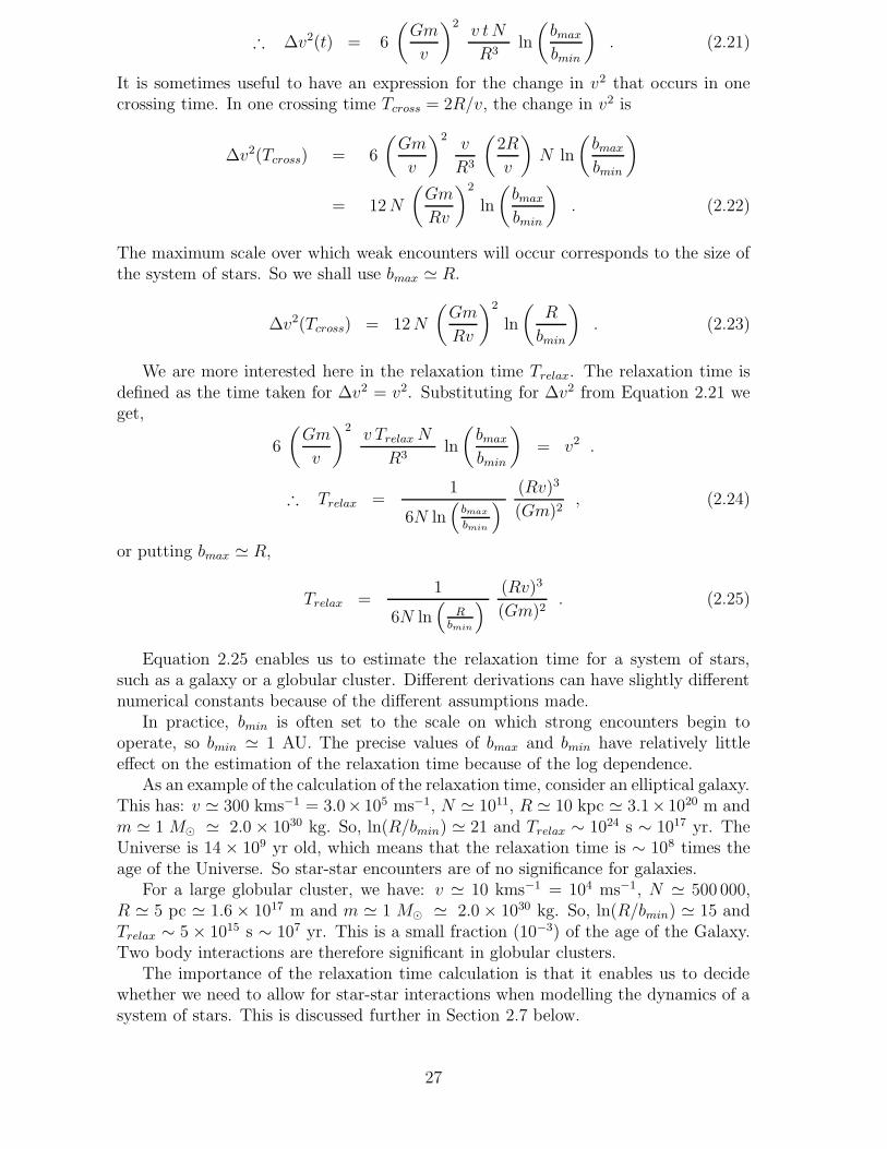
The orbit of a star in a spherical potential, to consider the simplest example, isconfined to a plane perpendicular to the angular momentum vector of the star. It is,however, not a closed path and has an appearance that is usually described as a rosette.In axisymmetric potentials (e.g. an oblate elliptical galaxy) the orbit is confined to aplane that precesses. This plane is inclined to the axis of symmetry and rotates aboutthe axis. The orbit within the plane is similar to that in a spherical potential.

Triaxial potentials can have orbits that are much more complex. Triaxial potentialsoften have the tendency to tumble about one axis, which leads to chaotic star orbits.

41

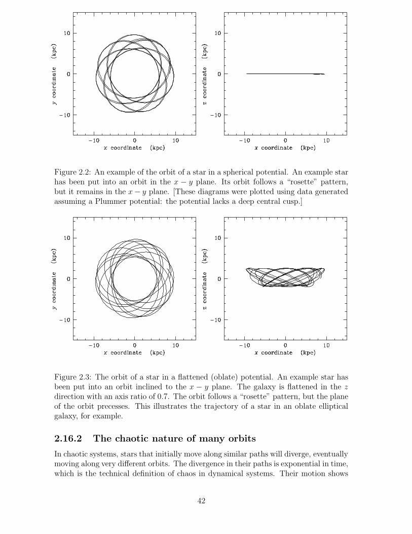
Figure 2.2: An example of the orbit of a star in a spherical potential. An example starhas been put into an orbit in the x − y plane. Its orbit follows a “rosette” pattern,but it remains in the x− y plane. [These diagrams were plotted using data generatedassuming a Plummer potential: the potential lacks a deep central cusp.]

Figure 2.3: The orbit of a star in a flattened (oblate) potential. An example star hasbeen put into an orbit inclined to the x − y plane. The galaxy is flattened in the zdirection with an axis ratio of 0.7. The orbit follows a “rosette” pattern, but the planeof the orbit precesses. This illustrates the trajectory of a star in an oblate ellipticalgalaxy, for example.

2.16.2 The chaotic nature of many orbits

In chaotic systems, stars that initially move along similar paths will diverge, eventuallymoving along very different orbits. The divergence in their paths is exponential in time,which is the technical definition of chaos in dynamical systems. Their motion shows

42

Figure 2.4: The orbit of a star in a triaxial potential. An example star has been putinto an orbit inclined to the x−y plane. The galaxy has different dimensions (differentscale sizes) in each of the x, y and z directions. The orbit is complex and it maps outa region of space. This illustrates the trajectory of a star in a triaxial elliptical galaxy,for example. (This simulation extends over a longer time period than those of Figures2.2 and 2.3.)

a stretching and folding in phase space. This can be so even if there is no collectivemotion of stars at all (f in equilibrium).

This stretching and folding in phase space can be appreciated using an analogy.When making bread, a baker’s dough behaves essentially as a fluid. Dough is in-compressible, but that does not prevent the baker stretching it in one direction andshrinking it in others, and then folding it back. So while the dough keeps much thesame overall shape, particles initially nearby within it can be dispersed to widely dif-ferent parts of it, through the repeated stretching and folding. The same stretchingand folding operation can take place for stars in phase space. In fact it appears thatphase space is typically riddled with regions where f gets stretched in one directionwhile being shrunk in others. Thus nearby orbits tend to diverge, and the divergenceis exponential in time.

Simulations show that the timescale for divergence (the e-folding time) is Tdiverge ∼Tcross, the crossing time, and gets shorter for higher star densities.

However, in some special cases, there is no chaos. These systems are said to beintegrable.

If the dynamics is confined to one real-space dimension (hence two phase-spacedimensions) then no stretching-and-folding can happen, and orbits are regular. So in aspherical system all orbits are regular. In addition, there are certain potentials (usuallyreferred to as Stackel potentials) where the dynamics decouples into three effectivelyone-dimensional systems; so if some equilibrium f generates a Stackel potential, theorbits will stay chaos-free. Also, small perturbations of non-chaotic systems tendto produce only small regions of chaos,1 and orbits may be well described through

1If you ever come across the ‘KAM theorem’, that’s basically it.

43

perturbation theory.

2.16.3 Integrals of the motion

To solve the collisionless Boltzmann equation for stars in a galaxy, we need furtherconstraints on the position and velocity. This can be done using integrals of the motion.These are simply functions of the star’s position x and velocity v that are constantalong its orbit. They are useful in potentials Φ(x) that are constant over time. Thedistribution function f is also constant along the orbit and can be written as a functionof integrals of the motion.

Examples of integrals of the motion are:

• The total energy. The mechanical energy E of a particular star in a potential isconstant over time, so E(x,v) = 1

2mv2 +mΦ(x). Because this is dependent on

the mass of the star, it is more normal to work with the energy per unit mass,which will be written as Em here. So Em = 1

2v2 + Φ is a constant.

• In an axisymmetric potential (e.g. our Galaxy), the z-component of the angularmomentum, Lz, is conserved. Therefore Lz is an integral of the motion in sucha potential.

• In a spherical potential, the total angular momentum L is constant. ThereforeL is an integral of the motion in this potential, and the x, y and z componentsof L are each integrals of the motion.

An orbit is said to be regular if it has as many isolating integrals that can definethe orbit unambiguously as there are spatial dimensions.

2.16.4 Isolating integrals and integrable systems

The collisionless Boltzmann equation tells us that df/dt = 0 (Section 2.14). As wasdiscussed earlier, if we move with a star in its orbit, f is constant locally as the starpasses through phase space at that instant in time. But if the system is in a steadystate (the potential is constant over time), f is constant along the star’s path at all

times. This means that the orbits of stars map out constant values of f .An integral of the motion for a star (e.g. energy per unit mass, Em) is constant

(by definition). They therefore define a 5-dimensional hypersurface in 6-dimensionalphase space. The motion of a star is confined to that 5-dimensional surface in phasespace. Therefore f is constant over that hypersurface.

A different value of the isolating integral (e.g. a different value of Em) will define adifferent hypersurface. In turn, f will be different on this surface. So f is a functionof the isolating integral, i.e. f(x, y, z, vx, vy, vz) = fn(I1) where I1 is an integral of themotion. I1 here “isolates” a hypersurface. Therefore the integral of the motion isknown as an isolating integral.

Integrals that fail to confine orbits are called “non-isolating” integrals. A systemis integrable if we can define isolating integrals that enable the orbit to be determined.

In integrable systems there are significant simplifications. Each orbit is (i) confinedto a three-dimensional toroidal subspace of six-dimensional phase space, and (ii) fills

44

its torus evenly.2 Phase space itself is filled by nested orbit-carrying tori—they have tobe nested, since orbits can’t cross in phase space. Therefore the time-average of eachorbit is completely specified once we have specified which torus it is on; this takes threenumbers for each orbit, and these are called ‘isolating integrals’ – they are constantsfor each orbit of course. Think of the isolating integrals as a coordinate system thatparameterises orbital tori; transformations to a different set of isolating integrals islike a coordinate transformation.

If isolating integrals exist, then any f that depends only on them will automaticallysatisfy the collisionless Boltzmann equation. Conversely, since orbits fill their torievenly, any equilibrium f cannot depend on location on the tori, it can only dependon the tori themselves, i.e., on the isolating integrals. This result is known as theJeans Theorem.

2.16.5 The Jeans Theorem

The Jeans Theorem is an important result in stellar dynamics that states the impor-tance of integrals of the motion in solving the collisionless Boltzmann equation forgravitational potentials that do not change with time. It was named after its discov-erer, the English astronomer, physicist and mathematician Sir James Hopwood Jeans(1877–1946). 3

It states that any steady-state solution of the collisionless Boltzmann equationdepends on the phase-space coordinates only through integrals of the motion in thegalaxy’s potential, and any function of the integrals yields a steady-state solution ofthe collisionless Boltzmann equation.

This means that in a potential that does not change with time, we can express thecollisionless Boltzmann equation in terms of integrals of motion, and then solve forthe distribution function f in terms of those integrals of motion. We can then convertthe solution of f in terms of the integrals to a solution for f in terms of the space andvelocity coordinates. For example, if the energy per unit mass Em and total angularmomentum components Lx and Ly are constant for each star in some potential, thenwe can solve for f uniquely as a function of Em, Lx and Ly. Then we can convert fromEm, Lx and Ly to give f as a function of (x, y, z, vx, vy, vz).

You should be wary of Jeans’ theorem, especially when people tacitly assume it,because as we saw, it assumes that the system is integrable, which is in general notthe case.

2.17 Spherical Systems

2.17.1 Solving for f in spherical galaxies

The Jeans Theorem does apply in spherical systems of stars, such as spherical ellipticalgalaxies. As a consequence, f can depend on (at most) three integrals of motion ina spherical system. The simplest case is for f to be a function of the energy of thestars only. (Since we are considering bound systems, f = 0 for E > 0 always: any

2These two statements are important results from Hamiltonian dynamical systems which we won’ttry to prove here. But the statements that follow in this section are straightforward consequences of(i) and (ii).

3Much of this work was published by Jeans in the Monthly Notices R.A.S., 76, 70, 1915.

45

stars that did have E > 0 will have escaped from the galaxy.) To find an equilibriumsolution, we only have to satisfy Poisson’s equation ∇2Φ = 4πGρ.

The total energy of a star of mass m moving with a velocity v is E = 12mv2 +mΦ,

where Φ is the gravitational potential at the point where the star is situated. Here itis more convenient to use the energy per unit mass Em = 1

2v2 + Φ.

A spherical galaxy can be described very simply by a spherical polar coordinatesystem (r, θ, φ) with the origin at the centre. Poisson’s equation relates the Laplacianof the gravitational potential Φ at a point to the local mass density ρ as ∇2Φ = 4πGρ.In a spherical polar coordinate system the Laplacian of any scalar function A(r, θ, φ)is

∇2A ≡ 1

r2

∂

∂r

(

r2 ∂A

∂r

)

+1

r2 sin θ

∂

∂θ

(

sin θ∂A

∂θ

)

+1

r2 sin2 θ

∂2A

∂φ2(2.63)

(a standard result from vector calculus: see Appendix C).In a spherically symmetric galaxy that does not change with time, the potential is

a function of the radial distance r from the centre only. So ∂Φ/∂θ = 0 and ∂Φ/∂φ = 0.Therefore,

∇2Φ =1

r2

d

dr

(

r2 dΦ

dr

)

. (2.64)

Substituting this into the Poisson equation,

1

r2

d

dr

(

r2 dΦ

dr

)

= 4πGρ . (2.65)

The distribution function f is related to the number density n of stars by

n =

∫

f d3v

(from Equation 2.39), and in this case f is a function of energy per unit mass: f =f(Em). We can relate this to the density ρ using ρ = m n where m is the mean massof a star, giving,

ρ = m

∫

f d3v . (2.66)

Note that here we are assuming that mass is in the form of stars only: there is no darkmatter here. This integral is over all velocities. We can convert from d3v to dv, wherev ≡ |v| by considering a thin spherical shell in a space defined by the three velocitycomponents, which gives d3v = 4πv2dv. So

ρ = 4π m

∫

fv2 dv . (2.67)

Note that this integration is over all velocities at a particular point in the galaxy. Itcan be performed over velocity at each and every point in the galaxy, so this ρ is ρ(r).(Here v is the magnitude of the velocity vector v, so v ≥ 0 always.)

We must determine the limits on this integral. For any particular point in thegalaxy (i.e. any value of r), the minimum possible velocity is v = 0, which occurswhen a star moving on a radial orbit reaches its maximum distance from the centreat that point. The maximum velocity at this position occurs when a star has thegreatest possible energy (Em = 0, which would allow a star to move out from the

46

point to arbitrary distance: any star with energy per unit mass Em > 0 will bemoving faster than the escape velocity for that location and will escape from thegalaxy). Therefore, using Em = 1

2v2 + Φ(r), the maximum velocity (for Em = 0) is

v =√

−2Φ(r) (remember that Φ(r) is negative, so that −2Φ(r) is positive). So the

integration at this point in space is from velocity v = 0 to√

−2Φ(r). So,

1

r2

d

dr

(

r2 dΦ

dr

)

= (4π)2 Gm

∫

√−2Φ(r)

0

f v2 dv . (2.68)

We can convert this integral over velocity to an integral over energy per unit mass.Em = 1

2v2 + Φ gives dEm = v dv at a fixed position (and hence for a constant Φ(r)).

The maximum possible energy per unit mass is 0 (because any stars with Em > 0 willhave escaped long ago), while the minimum possible value at a radius r would be givenby a star that is stationary at that point: Em = Φ(r) (which is of course negative).So, at any radius r,

1

r2

d

dr

(

r2 dΦ

dr

)

= (4π)2√

2 Gm

∫ 0

Φ(r)

√

Em − Φ(r) f(Em) dEm , (2.69)

on substituting v =√

2(Em − Φ) .It is usual in Equation 2.68 to take f(v) as given and to try to solve for Φ(r)

and hence ρ(r); this is a nonlinear differential equation. In Equation 2.69 we wouldnormally take Φ as given, and try to solve for f(Em); this is a linear integral equation.

There are f(Em) models in the literature, and you can always concoct a new oneby picking some ρ(r), computing Φ(r) and then solving Equation 2.69 numerically.Note that the velocity distribution is isotropic for any f(Em). If f depends on otherintegrals of motion, say angular momentum L or its z component, or both – thusf(Em, L

2, Lz) – then the velocity distribution will be anisotropic, and there are manyexamples of these around too.

2.17.2 Example of a spherical, isotropic distribution function:

the Plummer potential

As discussed earlier, the Plummer potential has a gravitational potential Φ and a massdensity ρ at a radial distance r from the centre that are given by

Φ(r) = − GMtot√r2 + a2

, ρ(r) =3Mtot

4π

a2

(r2 + a2)5/2, (2.32) and (2.33)

where Mtot is the total mass of the galaxy and a is a constant. The distributionfunction f for the Plummer model is related to the density ρ by Equation 2.67. It canbe shown that these Φ(r) and ρ(r) forms give a solution,

f(Em) =24√

2

7π3

a2

G5M4tot m

(−Em)72 . (2.70)

This can be verified by inserting in Equation 2.68, which can be done with somemathematical work. This result gives the distribution function f as a function only ofthe energy per unit mass Em. To calculate f for any point (x, y, z, vx, vy, vz) in phasespace, we need only to calculate Em from these coordinates and then calculate thevalue of f associated with that Em.

47

2.17.3 Example of a spherical, isotropic distribution function:the isothermal sphere

The isothermal sphere was introduced in Section 2.10.3. The density profile wasgiven in Equation 2.38. The isothermal sphere is defined by analogy with a Maxwell-Boltzmann gas, and therefore the distribution function as a function of the energy perunit mass Em is given by,

f(Em) =n0

(2πσ2)32

exp

(

− Em

σ2

)

=n0

(2πσ2)32

exp

(

−12v2 + Φ

σ2

)

, (2.71)

where σ is a velocity dispersion and acts in this distribution like a temperature doesin a gas. n0 is a constant. Integrating over velocities gives

n(r) =

∫

f d3v =

∫ ∞

0

f . 4π v2 dv =4π n0

(2πσ2)32

exp

(

− Φ

σ2

)∫ ∞

0

v2 exp

(

− v2

2σ2

)

dv

=4π n0

(2πσ2)32

exp

(

− Φ

σ2

)

.

(

σ3

4

√8π

)

= n0 exp

(

−Φ(r)

σ2

)

, (2.72)

using the standard integral∫∞

0x2e−ax2

dx =√

π/a3 /4 . (Note that the isothermaldistribution includes stars with speeds from v = 0 to ∞, so our integration is fromzero to infinity in this case, instead of the 0 to

√−2Φ used in the more realistic general

case in Equation 2.68. In practice, no stable galaxy will have stars with speeds largerthan

√

−2Φ(r) at a point a distance r from the centre because these stars would betravelling faster than escape velocity.)Converting this to density ρ(r) using ρ = mn, where m is the mean mass of the stars,we get,

ρ(r) = ρ0 exp

(

−Φ(r)

σ2

)

, and equivalently, Φ(r) = − σ2 ln

(

ρ(r)

ρ0

)

, (2.73)

where ρ0 is a constant (with ρ0 ≡ n0m). Using this, Poisson’s equation (∇2Φ = 4πGρ)in a spherically symmetric potential on substituting for dΦ/dr becomes,

1

r2

d

dr

(

r2 d

dr

(

− σ2 ln

(

ρ

ρ0

) ))

= 4πGρ ,

which simplifies tod

dr

(

r2 d ln ρ

dr

)

= − 4πG

σ2r2 ρ . (2.74)

This is a second-order differential equation in ρ and r. One solution to this is

ρ(r) =σ2

2πGr2, (2.38)

which is known as the singular isothermal sphere. As already commented in Sec-tion 2.10.3, the isothermal sphere has infinite mass! (A side effect of this is that theboundary condition Φ(∞) = 0 cannot be used, which is why we needed the redundant-looking constant ρ0 in Equations 2.71 and 2.72.) Nevertheless, this isothermal spheredensity profile is often used as a model, with some large-r truncation assumed, for thedark matter haloes of disc galaxies.

The same ρ(r) can be produced by many different f , all having different velocitydistributions.

48

2.18 Observable and Measurable Quantities

The phase space distribution f is usually very difficult to measure observationally,because of the challenges of measuring the distribution of stars over space and par-ticularly over velocity. Velocity components along the line of sight can be measuredspectroscopically from a Doppler shift. However, transverse velocity components can-not be measured directly for galaxies beyond our own (or at least beyond the LocalGroup). As a function of seven variables (six of the phase space, plus time), the func-tion f can be awkward to compute theoretically. It is therefore more convenient touse quantities related to f .

The number density n of stars in space can be measured observationally by count-ing more luminous stars for nearby galaxies, or from the observed intensity of light formore distant galaxies. Star counts combined with estimates of the distances of indi-vidual stars can provide n as a function of position within our Galaxy. For a distantgalaxy, converting the intensity along the line of sight of the integrated light from largenumbers of stars in to number densities – a process known as deprojection – requiresassumptions about the stellar populations and their three-dimensional distribution.Nevertheless, reasonable attempts can be made in many cases.

Spectroscopy provides mean velocities 〈vl〉 along the line of sight through a galaxy,and the widths of absorption lines provide velocity dispersions σl along the line of sight.These mean velocities will be weighted according to the numbers of stars. In our ownGalaxy, it is usually possible to calculate the mean velocity and the dispersions of thevelocity about the mean value.

The velocity dispersion is an important concept. Observational data can providethe velocity dispersion in perpendicular directions, at least within our own Galaxy. Soin our Galaxy, at each point in space, we might have the mean values of the velocitycomponents, 〈vR〉, 〈vφ〉 and 〈vz〉, in the R, φ and z directions, plus the dispersionsσR, σφ and σz, of the velocity components about their mean values, expressed as stan-dard deviations. Velocity dispersions are often represented by the velocity dispersion

ellipsoid. This is an idealised representation of the dispersions as a three-dimensionalellipsoid, where the distance from the origin in any particular direction is the size ofthe velocity dispersion in that direction.

When working with galaxies other than our own, we sometimes consider isotropic

velocity distributions (particularly for elliptical galaxies). In this case, the velocitydispersions in each direction are the same: σr = σθ = σφ, using a spherical coordinatesystem (r, θ, φ) here. We may abbreviate these equal components simply as σ, andthese will be the same as the velocity dispersion σl along our line of sight. If the meanvelocities are zero, i.e. 〈vr〉 = 〈vθ〉 = 〈vφ〉 = 0 (as will be the case if the galaxy is in asteady state and has no net rotation), then σ2 = 〈v2

r〉 = 〈v2θ〉 = 〈v2

φ〉. The mean of thesquare of the space velocity will be 〈v2〉 = 〈v2

r〉+ 〈v2θ〉+ 〈v2

φ〉. Therefore, 〈v2〉 = 3σ2 ina steady-state with no net rotation.

Although researchers often use the velocity dispersions in three perpendicular di-rections (such as σR, σφ and σz), a full description of the dynamics of stars requires avelocity dispersion tensor σij. This will discussed in detail later.

It is therefore much more convenient to calculate quantities involving number den-sities n, mean velocities and velocity dispersions from f . These quantities can thenbe compared with observations more directly. A series of equations called the JeansEquations allow this to be done.

49

2.19 The Jeans Equations

The Jeans Equations relate number densities, mean velocities, velocity dispersionsand the gravitational potential. They were first used in stellar dynamics by Sir JamesJeans in 1919.

It is useful to derive equations for the quantities

n =

∫

f d3v ,

n 〈vi〉 =

∫

vi f d3v ,

n σ 2ij =

∫

(vi − 〈vi〉) (vj − 〈vj〉) f d3v , (2.75)

by taking moments of the collisionless Boltzmann equation (expressed in the Cartesianvariables xi and vi). σij is a velocity dispersion tensor: it is discussed in more detailbelow.

The collisionless Boltzmann equation gives (Equation 2.46)

∂f

∂t+

3∑

i=1

(

dxi

dt

∂f

∂xi+

dvi

dt

∂f

∂vi

)

= 0 ,

or equivalently,

∂f

∂t+

3∑

i=1

vi∂f

∂xi−

3∑

i=1

∂Φ

∂xi

∂f

∂vi= 0 ,

on substituting for the components of acceleration from dv/dt = −∇Φ.To derive the first of the Jeans Equations, we shall consider the zeroth moment by

integrating this equation over all velocities.

∫

(

∂f

∂t+

3∑

i=1

vi∂f

∂xi−

3∑

i=1

∂Φ

∂xi

∂f

∂vi

)

d3v =

∫

0 . d3v . (2.76)

∴

∫

∂f

∂td3v +

3∑

i=1

∫

vi∂f

∂xi

d3v −3∑

i=1

∂Φ

∂xi

∫

∂f

∂vi

d3v = 0

(with the right hand being zero because it is a definite integral). Some of these termscan be simplified, particularly by noting the integration is performed over all velocitiesat each position and time.

50

But

∫

∂f

∂td3v =

∂

∂t

∫

f d3v because t and vi’s are independent

=∂n

∂tbecause n =

∫

f d3v,

and

∫

vi∂f

∂xid3v =

∫

∂(vif)

∂xid3v because vi’s and xi’s are independent

=∂

∂xi

∫

vi f d3v because xi’s and vi’s are independent

=∂ (n 〈vi〉 )

∂xion substituting n〈vi〉 =

∫

vifd3v

and

∫

∂Φ

∂xi

∂f

∂vi

d3v =∂Φ

∂xi

∫

∂f

∂vi

d3v because xi’s and Φ are independentof vi’s

=∂Φ

∂xi(0) because f −→ 0 as |vi| −→ ∞ (by analogy

with the divergence theorem)

= 0 .

Substituting for these terms,

∂n

∂t+

3∑

i=1

∂n〈vi〉∂xi

= 0 , (2.77)

which is a continuity equation. This is the first of the Jeans Equations.

To derive the second of the Jeans Equations, we consider the first moment ofthe collisionless Boltzmann equation by multiplying by vi and integrating over allvelocities. Multiplying the C.B.E. throughout by vi, we obtain,

vi∂f

∂t+ vi

3∑

j=1

vj∂f

∂xj− vi

3∑

j=1

∂Φ

∂xj

∂f

∂vj= 0 , (2.78)

where the summation is performed over an integer j because we have introduced avelocity component vi. Note that the use of vi means that we are considering oneparticular velocity component only at this stage, i.e. one value of i from i = 1, 3.Integrating this over all velocities,

∫

(

vi∂f

∂t+

3∑

j=1

vi vj∂f

∂xj−

3∑

j=1

vi∂Φ

∂xj

∂f

∂vj

)

d3v =

∫

0 . d3v . (2.79)

∴

∫

vi∂f

∂td3v +

3∑

j=1

∫

vi vj∂f

∂xjd3v −

3∑

j=1

∫

vi∂Φ

∂xj

∂f

∂vjd3v = 0 .

51

But

∫

vi∂f

∂td3v =

∫

∂(vi f)

∂td3v because vi and t are independent

=∂

∂t

∫

vi f d3v

=∂

∂t(n 〈vi〉) because n 〈vi〉 =

∫

vi f d3v,

and

∫

vi vj∂f

∂xj

d3v =

∫

∂

∂xj

(vi vj f) d3v because vi and vj are indepen-dent of xi

=∂

∂xj

∫

vivjf d3v because xi and vi’s are indepen-dent

=∂ (n 〈vivj〉 )

∂xj

on substituting n〈vivj〉 =∫

vivjf d3v

and

∫

vi∂Φ

∂xj

∂f

∂vjd3v =

∂Φ

∂xj

∫

vi∂f

∂vjd3v because xj’s and Φ are inde-

pendent of vi’s

But∂(vif)

∂vj

= vi∂f

∂vj

+ f∂vi

∂vj

∴ vi∂f

∂vj

=∂(vif)

∂vj

− f∂vi

∂vj

and∂vi

∂vj

= 1 if i = j

= 0 if i 6= j because vi and vj are independent if i 6= j

∴∂vi

∂vj

= δij

∴ vi∂f

∂vj=

∂(vif)

∂vj− δij f .

So

∫

vi∂Φ

∂xj

∂f

∂vj

d3v =∂Φ

∂xj

∫(

∂(vif)

∂vj

− δij f

)

d3v

=∂Φ

∂xj

(∫

∂(vif)

∂vj

d3v − δij

∫

f d3v

)

=∂Φ

∂xj

(

0 − δij n)

because vif −→ 0 as |vi| −→ ∞

= − ∂Φ

∂xj

δij n .

Substituting for these terms,

∂(n〈vi〉)∂t

+3∑

j=1

∂

∂xj

(

n〈vivj〉)

−3∑

j=1

(

− ∂Φ

∂xi

δij n

)

= 0 .

So,

∂(n〈vi〉)∂t

+

3∑

j=1

∂

∂xj

(

n〈vivj〉)

= − ∂Φ

∂xin , (2.80)

52

for each of i = 1, 2, 3. This is the second of the Jeans Equations.

We need to introduce a tensor velocity dispersion σij defined so that

n σ2ij ≡

∫

(

vi − 〈vi〉) (

vj − 〈vj〉)

f d3v , (2.81)

for i, j = 1, 3 (see Equation 2.75 above). This is used to represent the spread ofvelocities in each direction. It is a symmetric tensor and we can choose some coordinatesystem in which it is diagonal (i.e. σ11 6= 0, σ22 6= 0, σ33 6= 0, but all the otherelements are zero). This is known as the velocity ellipsoid. For example, in a cylindricalcoordinate system, we might use elements such as σRR, σφφ and σzz. If the velocitydispersion is isotropic, σ11 = σ22 = σ33, which we might simplify by writing as σ only.

Rearranging Equation 2.81 and multiplying out,

σ2ij =

1

n

∫

(

vi − 〈vi〉) (

vj − 〈vj〉)

f d3v

=1

n

∫

(

vivj − vi〈vj〉 − 〈vi〉vj + 〈vi〉 〈vj〉)

f d3v

=1

n

∫

vivj f d3v − 1

n

∫

vi 〈vj〉 f d3v − 1

n

∫

〈vi〉 vj f d3v

+1

n

∫

〈vi〉 〈vj〉 f d3v

=1

n

∫

vivj f d3v − 〈vj〉1

n

∫

vi f d3v − 〈vi〉1

n

∫

vj f d3v

+ 〈vi〉 〈vj〉1

n

∫

f d3v because 〈vi〉 and 〈vj〉 are constants

= 〈vivj〉 − 〈vj〉 〈vi〉 − 〈vi〉 〈vj〉 + 〈vi〉 〈vj〉 from Equation 2.75.

So,

σ2ij = 〈vivj〉 − 〈vi〉 〈vj〉 . (2.82)

This can be used to find 〈vivj〉 using

〈vivj〉 = σ2ij + 〈vi〉 〈vj〉 .

Substituting for 〈vivj〉 into the second of the Jeans Equations (Equation 2.80),

∂(n〈vi〉)∂t

+

3∑

j=1

[

∂

∂xj

(

nσ2ij

)

+∂

∂xj

(

n〈vi〉〈vj〉)

]

= − ∂Φ

∂xin ,

for each of i = 1, 2 and 3. Therefore,

〈vi〉∂n

∂t+ n

∂〈vi〉∂t

+

3∑

j=1

∂

∂xj

(

nσ2ij

)

+

3∑

j=1

∂

∂xj

(

n〈vi〉〈vj〉)

= − ∂Φ

∂xin . (2.83)

We can eliminate the 1st and 4th terms using the first of the Jeans Equations (Equa-tion 2.77). Multiplying that equation throughout by 〈vi〉,

〈vi〉∂n

∂t+ 〈vi〉

3∑

j=1

∂

∂xj

(

n〈vj〉)

= 0

∴ 〈vi〉∂n

∂t+

3∑

j=1

〈vi〉∂

∂xj

(

n〈vj〉)

= 0 (2.84)

53

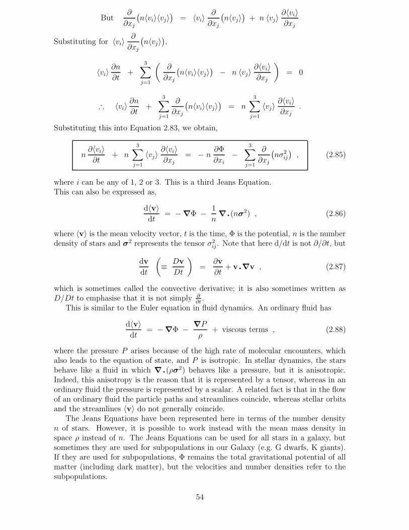
But∂

∂xj

(

n〈vi〉〈vj〉)

= 〈vi〉∂

∂xj

(

n〈vj〉)

+ n 〈vj〉∂〈vi〉∂xj

Substituting for 〈vi〉∂

∂xj

(

n〈vj〉)

,

〈vi〉∂n

∂t+

3∑

j=1

(

∂

∂xj

(

n〈vi〉〈vj〉)

− n 〈vj〉∂〈vi〉∂xj

)

= 0

∴ 〈vi〉∂n

∂t+

3∑

j=1

∂

∂xj

(

n〈vi〉〈vj〉)

= n3∑

j=1

〈vj〉∂〈vi〉∂xj

.

Substituting this into Equation 2.83, we obtain,

n∂〈vi〉∂t

+ n

3∑

j=1

〈vj〉∂〈vi〉∂xj

= − n∂Φ

∂xi−

3∑

j=1

∂

∂xj

(

nσ2ij

)

, (2.85)

where i can be any of 1, 2 or 3. This is a third Jeans Equation.This can also be expressed as,

d〈v〉dt

= − ∇Φ − 1

n∇.(nσ2) , (2.86)

where 〈v〉 is the mean velocity vector, t is the time, Φ is the potential, n is the numberdensity of stars and σ2 represents the tensor σ2

ij. Note that here d/dt is not ∂/∂t, but

dv

dt

(

≡ Dv

Dt

)

=∂v

∂t+ v.∇v , (2.87)

which is sometimes called the convective derivative; it is also sometimes written asD/Dt to emphasise that it is not simply ∂

∂t.

This is similar to the Euler equation in fluid dynamics. An ordinary fluid has

d〈v〉dt

= − ∇Φ − ∇P

ρ+ viscous terms , (2.88)

where the pressure P arises because of the high rate of molecular encounters, whichalso leads to the equation of state, and P is isotropic. In stellar dynamics, the starsbehave like a fluid in which ∇.(ρσ2) behaves like a pressure, but it is anisotropic.Indeed, this anisotropy is the reason that it is represented by a tensor, whereas in anordinary fluid the pressure is represented by a scalar. A related fact is that in the flowof an ordinary fluid the particle paths and streamlines coincide, whereas stellar orbitsand the streamlines 〈v〉 do not generally coincide.

The Jeans Equations have been represented here in terms of the number densityn of stars. However, it is possible to work instead with the mean mass density inspace ρ instead of n. The Jeans Equations can be used for all stars in a galaxy, butsometimes they are used for subpopulations in our Galaxy (e.g. G dwarfs, K giants).If they are used for subpopulations, Φ remains the total gravitational potential of allmatter (including dark matter), but the velocities and number densities refer to thesubpopulations.

54

2.20 The Jeans Equations in an Axisymmetric Sys-

tem, e.g. the Galaxy

Using cylindrical coordinates (R, φ, z) and assuming axisymmetry (so ∂/∂φ = 0), thesecond Jeans Equation is

∂

∂t

(

n〈vR〉)

+∂

∂R

(

n〈v2R〉)

+∂

∂z

(

n〈vRvz〉)

+n

R

(

〈v2R〉 − 〈v2

φ〉)

= − n∂Φ

∂Rfor the R direction,

∂

∂t

(

n〈vφ〉)

+∂

∂R

(

n〈vRvφ〉)

+∂

∂z

(

n〈vφvz〉)

+2n

R〈vRvφ〉 = 0

for the φ direction,

∂

∂t

(

n〈vz〉)

+∂

∂R

(

n〈vRvz〉)

+∂

∂z

(

n〈v2z〉)

+n 〈vRvz〉

R= − n

∂Φ

∂zfor the z direction. (2.89)

In a steady state, where the potential does not change with time, we can use∂/∂t = 0. This axisymmetric form of the second Jeans Equation is useful in spiralgalaxies, such as our own Galaxy, provided that we neglect any change in the potentialin the φ direction (although there might be a φ dependence if the potential is deeperin the spiral arms).

Meanwhile, the first of the Jeans Equations in a cylindrical coordinate system withaxisymmetric symmetry (∂/∂φ = 0) is,

∂n

∂t+

1

R

∂

∂R

(

Rn〈vR〉)

+∂

∂z

(

n〈vz〉)

= 0 . (2.90)

2.21 The Jeans Equations in a Spherically Sym-

metric System

The second Jeans Equation in a steady-state (∂/∂t = 0) spherically-symmetric (∂/∂φ =0, ∂/∂θ = 0) galaxy in a spherical polar coordinate system (r, θ, φ) is

d

dr

(

n 〈v2r〉)

+n

r

[

2〈v2r〉 − 〈v2

θ〉 − 〈v2φ〉]

= − ndΦ

dr. (2.91)

This might be used, for example, for a spherical elliptical galaxy.(This equation will just be stated here: it will not be derived. It can be derived

from the collisionless Boltzmann equation expressed in spherical coordinates usingsimilar methods to the Cartesian Jeans equations discussed above.)

We can calculate the gradient in the potential in this spherical case very simply.Using the general result that the acceleration due to gravity is g = −∇Φ, that g =GM(r)/r2 in a spherically symmetric system where M(r) is the mass interior to theradius r, and that ∇Φ = dΦ/dr in a spherical system, we get dΦ/dr = GM(r)/r2.

As a simple test to see whether this really does work, let us make a crude modelof our Galaxy’s stellar halo. We shall assume that the halo is spherical, assume alogarithmic potential of the form Φ(r) = v2

0 ln r where v0 is a constant, assume thatthe velocity components are isotropic (i.e. 〈v2

r〉 = 〈v2θ〉 = 〈v2

φ〉 = σ2, where σ is a

55

constant), and assume that the star number density of the halo can be approximatedby n(r) ∝ r−l where l is a constant. Equation 2.91 now becomes

d

dr

(

n σ2)

+n

r(0) = − n

dΦ

dr, ∴ σ2 dn

dr= −n

dΦ

dr,

on substituting for the velocity terms. Using Φ = v20 ln r and n(r) = kr−l (where k is

a constant) we get dΦ/dr = v20/r and dn/dr = −lkr−l−1. Substituting for these and

cancelling r, we obtain σ = v0/√l. For the Milky Way’s halo, observations show that

n ∝ r−3.5 (i.e. l = 3.5), while v0 as measured from gas on circular orbits is 220 km s−1,and rotation is negligible (which is a requirement for v2

θ = σ2 etc.). So we expectσ ' 220 km s−1/

√3.5 ' 120 km s−1. And it is.

2.22 Example of the Use of the Jeans Equations:

the Surface Mass Density of the Galactic Disc

The Jeans Equations can be applied to our Galaxy to measure the surface mass densityof the Galactic disc at the solar distance from the centre using observations of thevelocities of stars along the line of sight lying some distance above or below the Galacticplane. The surface mass density is the mass per unit area of the disc when viewedfrom from a great distance. It is expressed in units of kg m−2, or more commonly solarmasses per square parsec (M�pc−2). This analysis is important because it allows thequantity of dark matter in the disc to be estimated. Determining whether there isdark matter in the Galactic disc is a very important constraint on the nature of darkmatter.

56

The second Jeans Equation in a cylindrical coordinate system (R, φ, z) centred on theGalaxy, with z = 0 in the plane and R = 0 at the Galactic Centre states for the zdirection that

∂(n〈vz〉 )

∂t+

∂(n〈vRvz〉 )

∂R+

∂(n〈v2z〉 )

∂z+

n〈vRvz〉R

= − n∂Φ

∂z

(Equation 2.89), where n is the star number density, vR and vz are the velocity compo-nents in the R and z directions, Φ(R, z, t) is the Galactic gravitational potential andt is time.The Galaxy is in a steady state, so n does not change with time. Therefore the firstterm ∂(n〈vz〉)/∂t = 0.Observations show that

∂(n〈vRvz〉 )

∂R' 0 and

n〈vRvz〉R

' 0 ,

as is to be expected because of the cancelling of positive and negative terms of thez-components of the velocity. Therefore,

∂(n〈v2z〉 )

∂z= − n

∂Φ

∂z. (2.92)

〈v2z〉 is the mean square velocity in the direction perpendicular to the Galactic plane.

Poisson’s equation gives ∇2Φ = 4πGρ, where ρ is the mass density at a point. Incylindrical coordinates the Laplacian is

∇2Φ =1

R

∂

∂R

(

R∂Φ

∂R

)

+1

R2

∂2Φ

∂φ2+

∂2Φ

∂z2

(from Appendix C).If we observe stars directly above and below the Galactic plane, all at the same Galac-tocentric radius R, we can neglect the ∂Φ/∂R and ∂2Φ/∂φ2 terms.

∴∂2Φ

∂z2= 4πGρ ,

57

and substituting for ∂Φ/∂z from Equation 2.92 into this,

∂

∂z

(

− 1

n

∂

∂z

(

n〈v2z〉)

)

= 4πGρ .

Integrating perpendicular to the Galactic plane from −z to z, the surface mass densitywithin a distance z of the plane at a Galactocentric radius R is

Σ(R, z) =

∫ z

−z

ρ dz′ =

∫ z

−z

1

4πG

∂

∂z

(

− 1

n

∂

∂z

(

n〈v2z〉)

)

dz′

= − 1

4πG

[

1

n

∂

∂z

(

n〈v2z〉)

]z

z′=−z

= − 1

2πGn

∂

∂z

(

n〈v2z〉)

∣

∣

∣

∣

∣

z

,

assuming symmetry about z = 0. Therefore the surface mass density within a distancez of the plane at the solar Galactocentric radius R0 is

Σ(R0, z) = − 1

2πGn

∂

∂z

(

n〈v2z〉)

∣

∣

∣

∣

∣

z

. (2.93)

If the star densities n can be measured as a function of height z from the plane and ifthe z-component of the velocities vz can be measured as spectroscopic radial velocities,we can solve for Σ(R0, z) as a function of z. This gives, after modelling the contributionfrom the dark matter halo, the mass density of the Galactic disc.

The analysis can be performed on some subclass of stars, such as G giants or Kgiants. In this case the number density n of stars in space is that of the subclass.Number counts of stars towards the Galactic poles, combined with estimates of thedistances to individual stars, give n. Spectroscopic observations give radial velocities

58

(the velocity components along the line of sight) through the Doppler effect. Byobserving towards the Galactic poles, the radial velocities are the same as the vz

components.This analysis gives Σ(R0, z) as a function of z. The value increases with z as

a greater proportion of the stars of the disc are included, until all the disc matter isincluded. Σ(R0, z) will still increase slowly with z beyond this as an increasing amountmass from the dark matter halo is included. Indeed, it is necessary to determinethe contribution Σd(R0) from the disc alone to the observed data. An additionalcomplication is that in measuring ∂(n〈v2

z〉)/∂z as a function of z, we are dealing withthe differential of observed quantities. This means that the effects of observationalerrors can be considerable.

The first measurement of the surface density of the Galactic disc was carried outby Oort in 1932. More modern attempts were carried out in the 1980s by Bahcall andby Kuijken and Gilmore. There has been considerable debate about the interpretationof results. Early studies claimed evidence of dark matter in the Galactic disc, butmore recently some consensus has developed that there is little dark matter in the discitself, apart from the contribution from the dark matter halo that extends into thedisc. A modern value is Σd(R0) = 50 ± 10 M� pc−2. The absence of significant darkmatter in the disc indicates that dark matter does not follow baryonic matter closelyon a small scale, a very important result.

2.23 N-body Simulations

An alternative approach that can be adopted to study the dynamics of stars in galaxiesis to use N -body simulations. In these analyses, the system of stars is represented bya large number of particles and computer modelling is used to trace the dynamics ofthese particles under their mutual gravitational attractions. These simulations usuallydetermine the positions of the test particles at each of a series of time steps, calculatingthe changes in their positions between each step. It is possible to add further particlesto trace gas and dark matter, although the gas must be made collisional.

The individual particles in a galaxy simulation, however, do not correspond tostars. It is impossible to represent every star in a galaxy in N -body simulations. Inpractice, the limits on computational power allow only ∼ 105 to 108 particles, whereasthere may be as many as 1012 stars in the galaxies being modelled. The appropriateinterpretation of simulation particles is as Monte-Carlo samplers of the distributionfunction f .

In Section 2.6 we found that the ratio of the relaxation time to the crossing timewas Trelax/Tcross ∼ N/12 lnN for a system of N particles. It follows that a system thatis modelled computationally by too few particles will have a relaxation time that istoo short, and may experience the effects of two-body encounters. As a consequence,the particles in N -body simulations have to be made collisionless artificially. Thestandard way of doing this is to replace the 1/r gravitational potential of each particle

by (r2 +a2)−12 , which amounts to smearing out the mass on the ‘softening length’ scale

a.Early N -body computer codes performed calculations for each time step that took

a time that depended on the number N of particles as N 2. Modern codes performfaster computations by treating distant particles differently to nearby particles. “Treecodes” combine the effects of number of distant particles together. This increases their

59

efficiency and the computation times scale as only N lnN .N -body simulations are widely used now to study the evolution of galaxies, and an

active research area at present is to incorporate gas dynamics in them. In contrast tostandard N -body methods, smoothed particle hydrodynamics (SPH) are often usedto study the gas in galaxies. Modern simulations include the effects of dark matteralongside stars and gas. They can follow the collapse of clumps of dark matter inthe early Universe that led to the formation of galaxies. Simulations can also followthe growth of structure in the Universe as gravitational attraction produced the clus-tering of galaxies observed today. N -body simulations can model the effects of largechanges in gravitational potentials, whereas analytical methods can find these morechallenging.

60