stellar dynamics and structure of galaxies - collisionless...
TRANSCRIPT

Galaxies Part II
Collisionless Systems:Introduction
Relaxation time
Gravitational Drag /Focusing
The CollisionlessBoltzman Equation
The Jeans Equations
Application of Jeansequations
The Virial Theorem
Stellar Dynamics and Structure of GalaxiesCollisionless systems
Martin [email protected]
Institute of Astronomy
Michaelmas Term 2018
1 / 100

Galaxies Part II
Collisionless Systems:Introduction
Relaxation time
Gravitational Drag /Focusing
The CollisionlessBoltzman Equation
The Jeans Equations
Application of Jeansequations
The Virial Theorem
Outline I1 Collisionless Systems: Introduction
2 Relaxation time
3 Gravitational Drag / Focusing
4 The Collisionless Boltzman EquationThe Distribution FunctionPhase space flowThe fluid continuity equationThe continuity of flow in phase spaceIn cylindrical polarsLimitations and links with the real world
5 The Jeans EquationsZeroth momentFirst moment
6 Application of Jeans equationsIsotropic velocity dispersionJeans equations for cylindrically symmetric systemsApplication of axisymmetric Jeans equations
7 The Virial TheoremPotential-energy tensorKinetic-energy tensor
2 / 100

Galaxies Part II
Collisionless Systems:Introduction
Relaxation time
Gravitational Drag /Focusing
The CollisionlessBoltzman Equation
The Jeans Equations
Application of Jeansequations
The Virial Theorem
Outline IITensor Virial TheoremScalar Virial TheoremApplications Virial Theorem
3 / 100

Galaxies Part II
Collisionless Systems:Introduction
Relaxation time
Gravitational Drag /Focusing
The CollisionlessBoltzman Equation
The Jeans Equations
Application of Jeansequations
The Virial Theorem
Collisionless SystemsIntroduction
NB The use of the word “collisionless” is a technical one, specific tostellar dynamics. It does not simply mean there are no physicalcollisions between stars - it is a stronger statement than that.
Aiming to describe the strucure of a self-gravitating collection of stars,such as a star cluster or a galaxy.
e.g. globular cluster N ∼ 106 stars, rt ∼ 10 pc ∼ 3× 10¹⁷ m.
4 / 100

Galaxies Part II
Collisionless Systems:Introduction
Relaxation time
Gravitational Drag /Focusing
The CollisionlessBoltzman Equation
The Jeans Equations
Application of Jeansequations
The Virial Theorem
Collisionless SystemsIntroduction
1. Gravity is a long range force. For example, if the star density isuniform, then a star at the apex of a cone sees the same force from aregion of a given thickness independent of its distance.
m1 ∝ r 21 h
m2 ∝ r 22 h
and
f1 ∝ −Gm1
r 21
∝ h
f2 ∝ −Gm2
r 22
∝ h
⇒ the force acting on a star is determined by distant stars andlarge-scale structure of the galaxy. The force is zero if uniform densityeverywhere, but 6= 0 if the density falls off in one direction, forexample. This is unlike molecules of gas where forces are strong onlyduring close collisions
5 / 100

Galaxies Part II
Collisionless Systems:Introduction
Relaxation time
Gravitational Drag /Focusing
The CollisionlessBoltzman Equation
The Jeans Equations
Application of Jeansequations
The Virial Theorem
Collisionless SystemsIntroduction
2 Stars almost never collide physically.
Distance to nearest star in a globular cluster isd ∼ 10
(106)13∼ 0.1 pc ∼ 3× 10¹⁵ m >> r∗ ∼ 109 m.
r∗ d rt
This means that we can mentally smooth out the stars into a meandensity ρ and use that to calculate a mean gravitational potential Φand use that to calculate the orbits of the individual stars. The forceson a given star do not vary rapidly.
If this is a good approximation then the system is said to be“collisionless”..
6 / 100

Galaxies Part II
Collisionless Systems:Introduction
Relaxation time
Gravitational Drag /Focusing
The CollisionlessBoltzman Equation
The Jeans Equations
Application of Jeansequations
The Virial Theorem
Relaxation timeBetween 2 and ∞
N =∞ If the system consisted of an infinite number of stars whichare themselves point masses then the collisionless approximation wouldbe perfect.
N = 2 If instead we have a binary system then the approximation isdire - it does not work at all.
So somewhere between N = 2 and N =∞ it becomes OK. What isthe criterion for this?
Consider a system of N stars each of mass m, and look at the motionof one star as it crosses the system. Now look at
1 the path under the assumption that the mass of the stars issmoothed out
2 the real path using individual stars
What we want to do is estimate the difference between the two - or, inparticular, the difference in the resultant transverse (relative to theinitial motion) velocity of the star we have chosen to follow.
7 / 100

Galaxies Part II
Collisionless Systems:Introduction
Relaxation time
Gravitational Drag /Focusing
The CollisionlessBoltzman Equation
The Jeans Equations
Application of Jeansequations
The Virial Theorem
Relaxation timeWeak encounters
For the real path we will use an impulse approximation to start with.On the real path the star undergoes encounters with other stars whichperturb the straight path. One encounter with a star of mass m at(0, b), i.e. impact parameter b as shown:
on the path x = vt Fy =Gm2
r 2cos θ =
Gm2b
(x2 + b2)32
Fy =Gm2
b2
[1 +
(vtb
)2]− 3
2
= mvy
∆vy =Gm
b2
∫ ∞−∞
[1 +
(vtb
)2]− 3
2
dt
=Gm
bv
∫ ∞−∞
(1 + s2)−32 ds
Setting s = tan θ allows us to integrate this
∆vy =2Gm
bv
8 / 100

Galaxies Part II
Collisionless Systems:Introduction
Relaxation time
Gravitational Drag /Focusing
The CollisionlessBoltzman Equation
The Jeans Equations
Application of Jeansequations
The Virial Theorem
Relaxation timeWeak encounters
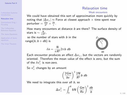
We could have obtained this sort of approximation more quickly bynoting that |∆v⊥| ≈ Force at closest approach × time spent nearperturber = Gm
b2 × 2bv
.
How many encounters at distance b are there? The surface density ofstars is ∼ N
πR2 ,
so the number of stars with b in therange(b, b + db) is
δn =N
πR22πb db
Each encounter produces an effect ∆v⊥, but the vectors are randomlyoriented. Therefore the mean value of the effect is zero, but the sumof the δv 2
⊥ is non-zero.
So v 2⊥ changes by an amount(
2Gm
bv
)22N
R2b db
We need to integrate this over all b, so
∆v 2⊥ =
∫ R
0
8N
(Gm
Rv
)2db
b9 / 100

Galaxies Part II
Collisionless Systems:Introduction
Relaxation time
Gravitational Drag /Focusing
The CollisionlessBoltzman Equation
The Jeans Equations
Application of Jeansequations
The Virial Theorem
Relaxation timeWeak encounters
We could have obtained this sort of approximation more quickly bynoting that |∆v⊥| ≈ Force at closest approach × time spent nearperturber = Gm
b2 × 2bv
.
How many encounters at distance b are there? The surface density ofstars is ∼ N
πR2 ,
so the number of stars with b in therange(b, b + db) is
δn =N
πR22πb db
Each encounter produces an effect ∆v⊥, but the vectors are randomlyoriented. Therefore the mean value of the effect is zero, but the sumof the δv 2
⊥ is non-zero.
So v 2⊥ changes by an amount(
2Gm
bv
)22N
R2b db
We need to integrate this over all b, so
∆v 2⊥ =
∫ R
0
8N
(Gm
Rv
)2db
b9 / 100

Galaxies Part II
Collisionless Systems:Introduction
Relaxation time
Gravitational Drag /Focusing
The CollisionlessBoltzman Equation
The Jeans Equations
Application of Jeansequations
The Virial Theorem
Relaxation timeWeak encounters
∆v 2⊥ =
∫ R
0
8N
(Gm
Rv
)2db
b
There is a problem here, and that is the lower limit 0 for the integral.The approximation we have used breaks down then, so replace 0 bybmin, the expected closest approach - i.e. such that
N
πR2(b2
minπ) = 1
sobmin ∼ R/N
12
Then
∆v 2⊥ ≈ 8N
(Gm
Rv
)2
ln Λ
where Λ = R/bmin.
10 / 100
Galaxies Part II
Collisionless Systems:Introduction
Relaxation time
Gravitational Drag /Focusing
The CollisionlessBoltzman Equation
The Jeans Equations
Application of Jeansequations
The Virial Theorem
Relaxation timeWeak encounters
Let us check for consistency that approximation we have used is OK.
When b = bmin. We have the requirement that δv⊥/v << 1,so require 2Gm/bv 2 << 1, or b >> 2Gm/v 2.
But from the Virial theorem v 2 ∼ GM/R ∼ GNm/R, so needb >> 2GmR/GNm = 2R/N, i.e. b/R >> 2/N.
For bmin have bmin/R ∼ 1/N12 >> 1/N, so the approximation is OK.
11 / 100
Galaxies Part II
Collisionless Systems:Introduction
Relaxation time
Gravitational Drag /Focusing
The CollisionlessBoltzman Equation
The Jeans Equations
Application of Jeansequations
The Virial Theorem
Relaxation timeThe time to erase the memory of the past motion
So we conclude that v 2⊥ changes by an amount ∆v 2
⊥ ≈ 8N(GmRv
)2ln Λ
at each crossing.
The collisionless approximation will fail after nrelax crossings, where
nrelax∆v 2⊥ ∼ v 2 i.e. nrelax8N
(Gm
Rv
)2
ln Λ ∼ v 2
and using v 2 ' GNmR
this becomes
nrelax8N
(v 2
Nv
)2
ln Λ ∼ v 2 i.e. nrelax ∼N
8 ln Λ
The relaxation time is
trelax = nrelax × tcross ≈ nrelaxR
v
and the crossing time
tcross ∼√
R3
GNm
12 / 100
Galaxies Part II
Collisionless Systems:Introduction
Relaxation time
Gravitational Drag /Focusing
The CollisionlessBoltzman Equation
The Jeans Equations
Application of Jeansequations
The Virial Theorem
Relaxation time
Notes:
1 ln Λ ∼ lnN, so nrelax ∼ N8 ln N
.
2 relaxation time is the timescale on which stars share energy witheach other.
3 can model a system as collisionless only if t << trelax.
Estimates of timescales:
• Galaxies: N ∼ 1011, tcross ∼ 108 yr, nrelax ∼ 5× 10⁸, sotrelax ∼ 5× 10⁸tcross ∼ 5× 10¹⁶ yr. This is much greater than aHubble time, so galaxies are not relaxed.
• Globular clusters: N ∼ 106, tcross ∼ 10pc/20km s−1 ∼ 5× 10⁵ yr,so trelax ∼ 4× 10⁹ yr. Their ages are somewhat greater than this,so globular clusters are relaxed, and hence spherical.
13 / 100

Galaxies Part II
Collisionless Systems:Introduction
Relaxation time
Gravitational Drag /Focusing
The CollisionlessBoltzman Equation
The Jeans Equations
Application of Jeansequations
The Virial Theorem
Gravitational Drag / Focusing
Consider a large mass M moving with speed v through a sea ofstationary masses m, density ρ. In the frame of the mass M:
.. so not only is v⊥affected, but there is also acontribution to v‖.
14 / 100

Galaxies Part II
Collisionless Systems:Introduction
Relaxation time
Gravitational Drag /Focusing
The CollisionlessBoltzman Equation
The Jeans Equations
Application of Jeansequations
The Virial Theorem
Gravitational Drag / Focusing
Relative to M have a Keplerian orbit with the angular momentumh = bv = r 2ψ The orbit, as you remember:
1
r= C cos(ψ − ψ0) +
GM
h2
15 / 100

Galaxies Part II
Collisionless Systems:Introduction
Relaxation time
Gravitational Drag /Focusing
The CollisionlessBoltzman Equation
The Jeans Equations
Application of Jeansequations
The Virial Theorem
Gravitational Drag / Focusing
1
r= C cos(ψ − ψ0) +
GM
h2
Get C , ψ0 by differentiatingthis ↑
dr
dt= Cr 2ψ sin(ψ − ψ0)
As ψ → 0 drdt→ −v so
−v = Cbv sin(−ψ0)
Also, since r →∞ then
0 = C cosψ0 +GM
b2v 2
sotanψ0 = −bv 2/GM
16 / 100

Galaxies Part II
Collisionless Systems:Introduction
Relaxation time
Gravitational Drag /Focusing
The CollisionlessBoltzman Equation
The Jeans Equations
Application of Jeansequations
The Virial Theorem
Gravitational Drag / Focusing
Now π − θdefl = 2(π − ψ0), soθdefl = 2ψ0 − π. ⇒
tan
(θdefl
2
)= − 1
tanψ0
and so
tan
(θdefl
2
)=
GM
bv 2
Then θdefl = π2
if ψ0 = 3π4
, or tanψ0 = −1 ⇒
b⊥ ∼GM
v 2
17 / 100

Galaxies Part II
Collisionless Systems:Introduction
Relaxation time
Gravitational Drag /Focusing
The CollisionlessBoltzman Equation
The Jeans Equations
Application of Jeansequations
The Virial Theorem
Gravitational Drag / Focusing
To estimate the drag force, we assume that all particles with b < b⊥lose all their momentum to M (i.e. δv ≈ v at b⊥)So the force on M = rate of change of momentum = πb2
⊥ρv2
(consider cylinder vdt × πb2 within which each star contributes v)So
Mdv
dt= −πρv 2
(GM
v 2
)2
ordv
dt' −πρG
2M
v 2
This is known as dynamical friction.
18 / 100

Galaxies Part II
Collisionless Systems:Introduction
Relaxation time
Gravitational Drag /Focusing
The CollisionlessBoltzman Equation
The Jeans Equations
Application of Jeansequations
The Virial Theorem
Gravitational Drag / Focusing
Note:
1 We have assumed that the mass is moving at velocity v withrespect to the background. In general the background will have avelocity dispersion σ. We have effectively assumed in the abovethat v >> σ. If v << σ then we expect negligible drag since theparticle barely “knows” it is moving. The general result (seeBinney & Tremaine, p643 onwards) is that drag is caused byparticles with velocities 0 < u < v .
2 Force F ∝ M2, and the wake mass is ∝ M
3 F ∝ 1v2 .
19 / 100

Galaxies Part II
Collisionless Systems:Introduction
Relaxation time
Gravitational Drag /Focusing
The CollisionlessBoltzman Equation
The Jeans Equations
Application of Jeansequations
The Virial Theorem
Gravitational Drag / FocusingNGC 2207
20 / 100
Galaxies Part II
Collisionless Systems:Introduction
Relaxation time
Gravitational Drag /Focusing
The CollisionlessBoltzman Equation
The Jeans Equations
Application of Jeansequations
The Virial Theorem
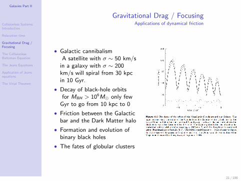
Gravitational Drag / FocusingApplications of dynamical friction
• Galactic cannibalismA satellite with σ ∼ 50 km/s
in a galaxy with σ ∼ 200km/s will spiral from 30 kpcin 10 Gyr.
• Decay of black-hole orbitsfor MBH > 106M only few
Gyr to go from 10 kpc to 0
• Friction between the Galacticbar and the Dark Matter halo
• Formation and evolution ofbinary black holes
• The fates of globular clusters
21 / 100

Galaxies Part II
Collisionless Systems:Introduction
Relaxation time
Gravitational Drag /Focusing
The CollisionlessBoltzman Equation
The Jeans Equations
Application of Jeansequations
The Virial Theorem
Gravitational Drag / FocusingSimulation of dwarf satellite accretion
22 / 100

Galaxies Part II
Collisionless Systems:Introduction
Relaxation time
Gravitational Drag /Focusing
The CollisionlessBoltzman Equation
The DistributionFunction
Phase space flow
The fluid continuityequation
The continuity of flow inphase space
In cylindrical polars
Limitations and linkswith the real world
The Jeans Equations
Application of Jeansequations
The Virial Theorem
The Collisionless Boltzman Equation
• If the interactions are rare, then the orbit of any star can becalculated as if the system’s mass was distributed smoothly.
• But, as we just saw, eventually the true orbit deviates from themodel orbit.
• Luckily, as long as we consider timescales < trelax we are fine
• In fact, for galaxies, trelax >> tHubble . Perfect!
• However, when modelling a collisionless system such as anelliptical galaxy it is not practical to follow the motions of allconstituent stars. Because there are too many of them!
23 / 100

Galaxies Part II
Collisionless Systems:Introduction
Relaxation time
Gravitational Drag /Focusing
The CollisionlessBoltzman Equation
The DistributionFunction
Phase space flow
The fluid continuityequation
The continuity of flow inphase space
In cylindrical polars
Limitations and linkswith the real world
The Jeans Equations
Application of Jeansequations
The Virial Theorem
The Collisionless Boltzman EquationThe Distribution Function
Let us assume that the stellar systems consist of a large number N ofidentical particles with mass m (could be stars, could be dark matter)moving under a smooth gravitational potential Φ(x, t).
Most problems are to do with working out the probability of finding astar in particular geographical location about the galaxy, moving at aparticular speed.
Or, in other words, the probability of finding the star in thesix-dimensional phase-space volume d3xd3v, which is a small volumed3x centred on x in the small velocity range d3v centred on v.
At any time t a full description of the state of this system is given byspecifying the number of stars f (x, v, t)d3xd3v, where f (x, v, t) iscalled the “distribution function” (or “phase space density”) of thesystem.
Obviously, f ≥ 0 everywhere, since we do not allow negative stardensities.
24 / 100

Galaxies Part II
Collisionless Systems:Introduction
Relaxation time
Gravitational Drag /Focusing
The CollisionlessBoltzman Equation
The DistributionFunction
Phase space flow
The fluid continuityequation
The continuity of flow inphase space
In cylindrical polars
Limitations and linkswith the real world
The Jeans Equations
Application of Jeansequations
The Virial Theorem
The Collisionless Boltzman EquationThe Distribution Function
Naturally, integrating over all phase space:∫f (x, v, t)d3xd3v = N (5.1)
Alternatively, we can normalize it to have:∫f (x, v, t)d3xd3v = 1 (5.2)
Then f (x, v, t)d3xd3v is the probability that at time t a randomlychosen star has phase-space coordinates in the given range.
25 / 100

Galaxies Part II
Collisionless Systems:Introduction
Relaxation time
Gravitational Drag /Focusing
The CollisionlessBoltzman Equation
The DistributionFunction
Phase space flow
The fluid continuityequation
The continuity of flow inphase space
In cylindrical polars
Limitations and linkswith the real world
The Jeans Equations
Application of Jeansequations
The Virial Theorem
The Collisionless Boltzman EquationPhase space flow
If we know the initial coordinates and velocities of every star, then wecan use Newton’s laws to evaluate their positions and velocities at anyother time i.e. given f (x, v, t0) then we should be able to determinef (x, v, t) for any t. With this aim, we consider the flow of points inphase space, with coordinates (x,v), that arises as stars move along intheir orbits. We can set the phase space coordinates
(x, v) ≡ w ≡ (w1,w2,w3,w4,w5,w6)
so the velocity of the flow (which is the time derivative of thecoordinates) may be written as
w = (x, v) = (v,−∇Φ).
w is a six-dimensional vector which bears the same relationship to thesix-dimensional vector w as the three-dimensional fluid flow velocityv = x.
26 / 100

Galaxies Part II
Collisionless Systems:Introduction
Relaxation time
Gravitational Drag /Focusing
The CollisionlessBoltzman Equation
The DistributionFunction
Phase space flow
The fluid continuityequation
The continuity of flow inphase space
In cylindrical polars
Limitations and linkswith the real world
The Jeans Equations
Application of Jeansequations
The Virial Theorem
The Collisionless Boltzman EquationPhase space flow
Any given star moves through phase space, so the probability of findingit at any given phase-space location changes with time. In what way?
However, the flow in phase space conserves stars, hence we can derivethe equation of conservation of the phase space probability analogousto the fluid continuity equation.
27 / 100

Galaxies Part II
Collisionless Systems:Introduction
Relaxation time
Gravitational Drag /Focusing
The CollisionlessBoltzman Equation
The DistributionFunction
Phase space flow
The fluid continuityequation
The continuity of flow inphase space
In cylindrical polars
Limitations and linkswith the real world
The Jeans Equations
Application of Jeansequations
The Virial Theorem
The Collisionless Boltzman EquationThe fluid continuity equation
For an arbitrary closed volume V fixed in space and bounded bysurface S , the mass of fluid in the volume is
M(t) =
∫V
d3xρ(x, t) (5.3)
The fluid mass changes with time at a rate
dM
dt=
∫V
d3x∂ρ
∂t(5.4)
But, the mass flowing out through the surface area element d2S perunit time ρv · d2S. Thus:
dM
dt= −
∮S
d2S · (ρv) (5.5)
Or ∫V
d3x∂ρ
∂t+
∮S
d2S · (ρv) = 0 (5.6)
28 / 100

Galaxies Part II
Collisionless Systems:Introduction
Relaxation time
Gravitational Drag /Focusing
The CollisionlessBoltzman Equation
The DistributionFunction
Phase space flow
The fluid continuityequation
The continuity of flow inphase space
In cylindrical polars
Limitations and linkswith the real world
The Jeans Equations
Application of Jeansequations
The Virial Theorem
∫V
d3x∂ρ
∂t+
∮S
d2S · (ρv) = 0
can be re-written with the use of the divergence theorem:∫V
d3x
[∂ρ
∂t+ ∇ · (ρv)
]= 0 (5.7)
Since the result holds for any volume:
∂ρ
∂t+ ∇ · (ρv) = 0 (5.8)
Which in Cartesian coordinates looks like this:
∂ρ
∂t+
∂
∂xj(ρvj) = 0 (5.9)
using the summation convention
A · B =3∑
i=1
AiBi = AiBi
29 / 100

Galaxies Part II
Collisionless Systems:Introduction
Relaxation time
Gravitational Drag /Focusing
The CollisionlessBoltzman Equation
The DistributionFunction
Phase space flow
The fluid continuityequation
The continuity of flow inphase space
In cylindrical polars
Limitations and linkswith the real world
The Jeans Equations
Application of Jeansequations
The Virial Theorem
The Collisionless Boltzman EquationThe continuity of flow in phase space
Since x = v , for fluids:
∂ρ
∂t+
∂
∂x· (f x) = 0
The analogous equation for the conservation of probability in phasespace is:
∂f
∂t+
∂
∂w· (f w) = 0 (5.10)
Note that writing it as a continuity equation carries with it theassumption that the function f is differentiable. This means that closestellar encounters where a star can jump from one point in phasespace to another are excluded from this description.
30 / 100

Galaxies Part II
Collisionless Systems:Introduction
Relaxation time
Gravitational Drag /Focusing
The CollisionlessBoltzman Equation
The DistributionFunction
Phase space flow
The fluid continuityequation
The continuity of flow inphase space
In cylindrical polars
Limitations and linkswith the real world
The Jeans Equations
Application of Jeansequations
The Virial Theorem
The Collisionless Boltzman EquationThe continuity of flow in phase space
Let us have a closer look at the second term in ∂f∂t
+ ∂∂w · (f w)= 0
∂(f wi )
∂wi= wi
∂f
∂wi+ f
∂wi
∂wi(5.11)
The flow in six-space is an interesting one, since
6∑i=1
∂(wi )
∂wi=
3∑i=1
(∂vi∂xi
+∂vi∂vi
)=
3∑i=1
− ∂
∂vi
(∂Φ
∂xi
)= 0 (5.12)
Here ∂vi∂xi
= 0 because in this space vi and xi are independentcoordinates, and the last step follows because Φ, and hence ∇Φ doesnot depend on the velocities. We can use this equation to simplify thecontinuity equation, which now becomes
∂f
∂t+
6∑i=1
wi∂f
∂wi= 0 (5.13)
31 / 100
Galaxies Part II
Collisionless Systems:Introduction
Relaxation time
Gravitational Drag /Focusing
The CollisionlessBoltzman Equation
The DistributionFunction
Phase space flow
The fluid continuityequation
The continuity of flow inphase space
In cylindrical polars
Limitations and linkswith the real world
The Jeans Equations
Application of Jeansequations
The Virial Theorem
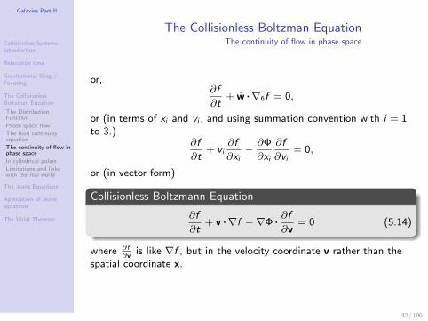
The Collisionless Boltzman EquationThe continuity of flow in phase space
or,∂f
∂t+ w .∇6f = 0,
or (in terms of xi and vi , and using summation convention with i = 1to 3.)
∂f
∂t+ vi
∂f
∂xi− ∂Φ
∂xi
∂f
∂vi= 0,
or (in vector form)
Collisionless Boltzmann Equation
∂f
∂t+ v .∇f −∇Φ . ∂f
∂v= 0 (5.14)
where ∂f∂v is like ∇f , but in the velocity coordinate v rather than the
spatial coordinate x.
32 / 100

Galaxies Part II
Collisionless Systems:Introduction
Relaxation time
Gravitational Drag /Focusing
The CollisionlessBoltzman Equation
The DistributionFunction
Phase space flow
The fluid continuityequation
The continuity of flow inphase space
In cylindrical polars
Limitations and linkswith the real world
The Jeans Equations
Application of Jeansequations
The Virial Theorem
The Collisionless Boltzman EquationLiouville’s Theorem
The meaning of the collisionless Boltzmann equation can be seen byextending to six dimensions the concept of the Lagrangian derivative.We define (using the summation convention here and forever more)
Df
Dt≡ ∂f
∂t+ wi
∂f
∂wi(5.15)
dfdt
represents the rate of change of density in phase space as seen byan observer who moves through phase space with a star with phasespace velocity w. The collisionless Boltzmann equation is then simply
Df
Dt= 0 (5.16)
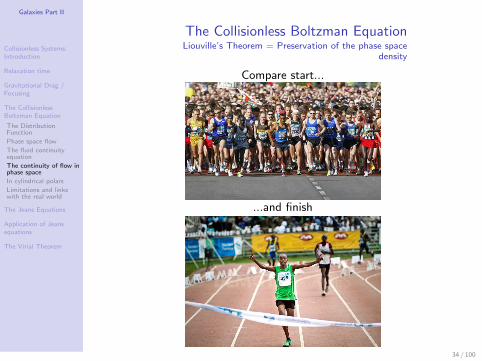
Therefore the flow of stellar phase points through phase space isincompressible – the phase-space density of points around a given staris always the same.
33 / 100
Galaxies Part II
Collisionless Systems:Introduction
Relaxation time
Gravitational Drag /Focusing
The CollisionlessBoltzman Equation
The DistributionFunction
Phase space flow
The fluid continuityequation
The continuity of flow inphase space
In cylindrical polars
Limitations and linkswith the real world
The Jeans Equations
Application of Jeansequations
The Virial Theorem
The Collisionless Boltzman EquationLiouville’s Theorem = Preservation of the phase space
density
Compare start...
...and finish
34 / 100

Galaxies Part II
Collisionless Systems:Introduction
Relaxation time
Gravitational Drag /Focusing
The CollisionlessBoltzman Equation
The DistributionFunction
Phase space flow
The fluid continuityequation
The continuity of flow inphase space
In cylindrical polars
Limitations and linkswith the real world
The Jeans Equations
Application of Jeansequations
The Virial Theorem
The Collisionless Boltzman EquationLiouville’s Theorem = Preservation of the phase space
density
35 / 100

Galaxies Part II
Collisionless Systems:Introduction
Relaxation time
Gravitational Drag /Focusing
The CollisionlessBoltzman Equation
The DistributionFunction
Phase space flow
The fluid continuityequation
The continuity of flow inphase space
In cylindrical polars
Limitations and linkswith the real world
The Jeans Equations
Application of Jeansequations
The Virial Theorem
The Collisionless Boltzman EquationLiouville’s Theorem = Preservation of the phase space
density
36 / 100

Galaxies Part II
Collisionless Systems:Introduction
Relaxation time
Gravitational Drag /Focusing
The CollisionlessBoltzman Equation
The DistributionFunction
Phase space flow
The fluid continuityequation
The continuity of flow inphase space
In cylindrical polars
Limitations and linkswith the real world
The Jeans Equations
Application of Jeansequations
The Virial Theorem
The Collision-less Boltzman EquationLiouville’s Theorem = Preservation of the phase space
density
37 / 100

Galaxies Part II
Collisionless Systems:Introduction
Relaxation time
Gravitational Drag /Focusing
The CollisionlessBoltzman Equation
The DistributionFunction
Phase space flow
The fluid continuityequation
The continuity of flow inphase space
In cylindrical polars
Limitations and linkswith the real world
The Jeans Equations
Application of Jeansequations
The Virial Theorem
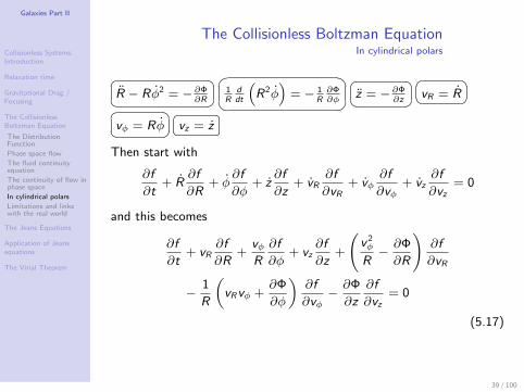
The Collisionless Boltzman EquationIn cylindrical polars
Be careful when writing down the collisionless Boltzmann equation innon-Cartesian coordinates! For example, in cylindrical polars (axialsymmetry)
R − Rφ2 = −∂Φ
∂R
1
R
d
dt
(R2φ
)= − 1
R
∂Φ
∂φ
z = −∂Φ
∂z
withvR = R
vφ = Rφ ( not just φ)
vz = z
Since dx = dReR + Rdφeφ + dzez
38 / 100
Galaxies Part II
Collisionless Systems:Introduction
Relaxation time
Gravitational Drag /Focusing
The CollisionlessBoltzman Equation
The DistributionFunction
Phase space flow
The fluid continuityequation
The continuity of flow inphase space
In cylindrical polars
Limitations and linkswith the real world
The Jeans Equations
Application of Jeansequations
The Virial Theorem
The Collisionless Boltzman EquationIn cylindrical polars R − Rφ2 = − ∂Φ
∂R
1
Rddt
(R2φ
)= − 1
R∂Φ∂φ
z = − ∂Φ∂z
vR = R vφ = Rφ vz = z
Then start with
∂f
∂t+ R
∂f
∂R+ φ
∂f
∂φ+ z
∂f
∂z+ vR
∂f
∂vR+ vφ
∂f
∂vφ+ vz
∂f
∂vz= 0
and this becomes
∂f
∂t+ vR
∂f
∂R+
vφR
∂f
∂φ+ vz
∂f
∂z+
(v 2φ
R− ∂Φ
∂R
)∂f
∂vR
− 1
R
(vRvφ +
∂Φ
∂φ
)∂f
∂vφ− ∂Φ
∂z
∂f
∂vz= 0
(5.17)
39 / 100

Galaxies Part II
Collisionless Systems:Introduction
Relaxation time
Gravitational Drag /Focusing
The CollisionlessBoltzman Equation
The DistributionFunction
Phase space flow
The fluid continuityequation
The continuity of flow inphase space
In cylindrical polars
Limitations and linkswith the real world
The Jeans Equations
Application of Jeansequations
The Virial Theorem
The Collisionless Boltzman EquationLimitations and links with the real world
1 Stars are born and die! Hence they are not really conserved.Therefore, more appropriately:
Df
Dt=∂f
∂t+ v
∂f
∂x− ∂Φ
∂x
∂f
∂v= B − D (5.18)
where B(x, v, t) and D(x, v, t) are the rates per unit phase-spacevolume at which stars are born and die.
But v∂f /∂x ≈ vf /R = f /tcross
Similarly, ∂Φ/∂x ≈ a ≈ v/tcross , hence∂Φ/∂x ∂f /∂v ≈ af /v ≈ f /tcrossTherefore, the important ratio
γ =
∣∣∣∣B − D
f /tcross
∣∣∣∣ 1 (5.19)
i.e. the fractional change in the number of stars per crossing time issmall
40 / 100

Galaxies Part II
Collisionless Systems:Introduction
Relaxation time
Gravitational Drag /Focusing
The CollisionlessBoltzman Equation
The DistributionFunction
Phase space flow
The fluid continuityequation
The continuity of flow inphase space
In cylindrical polars
Limitations and linkswith the real world
The Jeans Equations
Application of Jeansequations
The Virial Theorem
The Collisionless Boltzman EquationLimitations and links with the real world
Density of stars at a particular location x
ν(x) ≡∫
d3vf (x, v) (5.20)
Probability distribution of stellar velocities at x
Px(v) =f (x, v)
ν(x)(5.21)
For lines of sight through the galaxy, defined by s - a unit vector fromobserver to the galaxy.The components of x and v vectors parallel and perpendicular to theline of sight are:
x‖ ≡ s · x
v‖ ≡ s · v
x⊥ ≡ x− x‖s
v⊥ ≡ v − v‖s
41 / 100
Galaxies Part II
Collisionless Systems:Introduction
Relaxation time
Gravitational Drag /Focusing
The CollisionlessBoltzman Equation
The DistributionFunction
Phase space flow
The fluid continuityequation
The continuity of flow inphase space
In cylindrical polars
Limitations and linkswith the real world
The Jeans Equations
Application of Jeansequations
The Virial Theorem
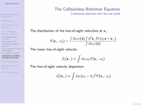
The Collisionless Boltzman EquationLimitations and links with the real world
The distribution of the line-of-sight velocities at x⊥
F (x⊥, v‖) =
∫dx‖ν(x)
∫d2v⊥Px(v‖s + v⊥)∫dx‖ν(x)
The mean line-of-sight velocity:
v‖(x⊥) ≡∫
dv‖v‖F (x⊥, v‖)
The line-of-sight velocity dispersion:
σ2‖(x⊥) ≡
∫dv‖(v‖ − v‖)
2F (x⊥, v‖)
42 / 100
Galaxies Part II
Collisionless Systems:Introduction
Relaxation time
Gravitational Drag /Focusing
The CollisionlessBoltzman Equation
The Jeans Equations
Zeroth moment
First moment
Application of Jeansequations
The Virial Theorem
The Jeans Equations
• The distribution function f is a function of seven variables, sosolving the collisionless Boltzmann equation in general is hard.
• So need either simplifying assumptions (usually symmetry), or tryto get insights by taking moments of the equation.
• We cannot observe f , but can determine ρ and line profile (which
is the average velocity along a line of sight v r and v 2r .
43 / 100

Galaxies Part II
Collisionless Systems:Introduction
Relaxation time
Gravitational Drag /Focusing
The CollisionlessBoltzman Equation
The Jeans Equations
Zeroth moment
First moment
Application of Jeansequations
The Virial Theorem
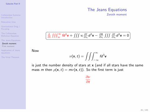
The Jeans EquationsZeroth moment
Start with the collisionless Boltzmann equation -using the summationconvention
∂f
∂t+ vi
∂f
∂xi− ∂Φ
∂xi
∂f
∂vi= 0 (5.22)
and take the zeroth moment integrating over d3v.
∂
∂t
∫ ∫ ∫ ∞∞
fd3v +
∫ ∫ ∫vi∂f
∂xid3v − ∂Φ
∂xi
∫ ∫ ∫∂f
∂vid3v = 0 (5.23)
where for the first term we can take the differential with respect totime out of the integral since the limits are independent of t, and inthe third term Φ is independent of v so the ∂Φ
∂xiterm comes out.
44 / 100
Galaxies Part II
Collisionless Systems:Introduction
Relaxation time
Gravitational Drag /Focusing
The CollisionlessBoltzman Equation
The Jeans Equations
Zeroth moment
First moment
Application of Jeansequations
The Virial Theorem
The Jeans EquationsZeroth moment
∂∂t
∫∫∫∞∞ fd3v +
∫∫∫vi∂f∂xi
d3v − ∂Φ∂xi
∫∫∫∂f∂vi
d3v = 0
Now
ν(x, t) =
∫ ∫ ∫ ∞−∞
fd3v
is just the number density of stars at x (and if all stars have the samemass m then ρ(x, t) = mν(x, t)). So the first term is just
∂ν
∂t
45 / 100

Galaxies Part II
Collisionless Systems:Introduction
Relaxation time
Gravitational Drag /Focusing
The CollisionlessBoltzman Equation
The Jeans Equations
Zeroth moment
First moment
Application of Jeansequations
The Virial Theorem
The Jeans EquationsZeroth moment
∂∂t
∫∫∫∞∞ fd3v +
∫∫∫vi∂f∂xi
d3v − ∂Φ∂xi
∫∫∫∂f∂vi
d3v = 0
Also∂
∂xi(vi f ) =
∂vi∂xi
f + vi∂f
∂xi
and∂vi∂xi
= 0
since vi and xi are independent coordinates, and so
∂
∂xi(vi f ) = vi
∂f
∂xi
46 / 100

Galaxies Part II
Collisionless Systems:Introduction
Relaxation time
Gravitational Drag /Focusing
The CollisionlessBoltzman Equation
The Jeans Equations
Zeroth moment
First moment
Application of Jeansequations
The Virial Theorem
The Jeans EquationsZeroth moment
∂∂t
∫∫∫∞∞ fd3v +
∫∫∫vi∂f∂xi
d3v − ∂Φ∂xi
∫∫∫∂f∂vi
d3v = 0
Hence the second term above becomes
∂
∂xi
∫ ∫ ∫vi fd
3v
and if we define an average velocity v i by
v i =1
ν
∫ ∫ ∫vi fd
3v
(so interpret f as a probability density) then the term we areconsidering becomes
∂
∂xi(νv i )
47 / 100
Galaxies Part II
Collisionless Systems:Introduction
Relaxation time
Gravitational Drag /Focusing
The CollisionlessBoltzman Equation
The Jeans Equations
Zeroth moment
First moment
Application of Jeansequations
The Virial Theorem
The Jeans EquationsZeroth moment
∂∂t
∫∫∫∞∞ fd3v +
∫∫∫vi∂f∂xi
d3v − ∂Φ∂xi
∫∫∫∂f∂vi
d3v = 0
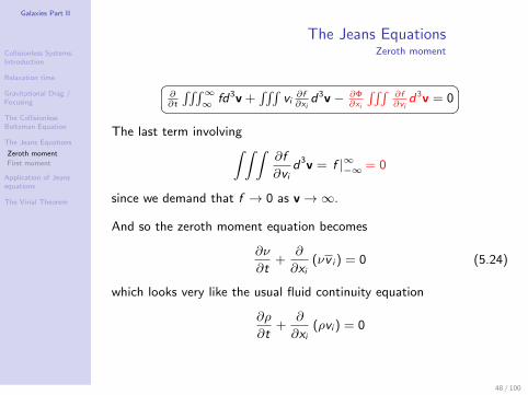
The last term involving∫ ∫ ∫∂f
∂vid3v = f |∞−∞= 0
since we demand that f → 0 as v→∞.
And so the zeroth moment equation becomes
∂ν
∂t+
∂
∂xi(νv i ) = 0 (5.24)
which looks very like the usual fluid continuity equation
∂ρ
∂t+
∂
∂xi(ρvi ) = 0
48 / 100
Galaxies Part II
Collisionless Systems:Introduction
Relaxation time
Gravitational Drag /Focusing
The CollisionlessBoltzman Equation
The Jeans Equations
Zeroth moment
First moment
Application of Jeansequations
The Virial Theorem
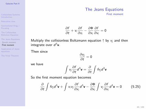
The Jeans EquationsFirst moment
∂f
∂t+ vi
∂f
∂xi− ∂Φ
∂xi
∂f
∂vi= 0
Multiply the collisionless Boltzmann equation ↑ by vj and thenintegrate over d3v.
Then since∂vj∂t
= 0
we have ∫vj∂f
∂td3v =
∂
∂t
∫fvjd
3v
So the first moment equation becomes
∂
∂t
∫fvjd
3v +
∫vivj
∂f
∂xid3v − ∂Φ
∂xi
∫vj∂f
∂vid3v = 0 (5.25)
49 / 100
Galaxies Part II
Collisionless Systems:Introduction
Relaxation time
Gravitational Drag /Focusing
The CollisionlessBoltzman Equation
The Jeans Equations
Zeroth moment
First moment
Application of Jeansequations
The Virial Theorem
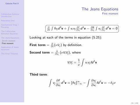
The Jeans EquationsFirst moment
∂∂t
∫fvjd
3v +∫vivj
∂f∂xi
d3v − ∂Φ∂xi
∫vj∂f∂vi
d3v = 0
Looking at each of the terms in equation (5.25):
First term = ∂∂t
(νv j) by definition.
Second term = ∂∂xi
(νvivj), where
vivj =1
ν
∫vivj fd
3v
Third term: ∫vj∂f
∂vid3v = [fvj ]
∞−∞ −
∫∂vj∂vi
fd3v = −δijν
50 / 100

Galaxies Part II
Collisionless Systems:Introduction
Relaxation time
Gravitational Drag /Focusing
The CollisionlessBoltzman Equation
The Jeans Equations
Zeroth moment
First moment
Application of Jeansequations
The Virial Theorem
The Jeans EquationsFirst moment
∂∂t
∫fvjd
3v +∫vivj
∂f∂xi
d3v − ∂Φ∂xi
∫vj∂f∂vi
d3v = 0
So first moment equation is
∂
∂t(νv j) +
∂
∂xi(νvivj) + ν
∂Φ
∂xj= 0 (5.26)
We can manipulate this a bit further - subtracting
v j× ∂ν∂t
+ ∂∂xi
(νv i ) = 0
gives
ν∂v j
∂t− v j
∂
∂xi(νvi ) +
∂
∂xi(νvivj) = −ν ∂Φ
∂xj(5.27)
51 / 100

Galaxies Part II
Collisionless Systems:Introduction
Relaxation time
Gravitational Drag /Focusing
The CollisionlessBoltzman Equation
The Jeans Equations
Zeroth moment
First moment
Application of Jeansequations
The Virial Theorem
The Jeans EquationsFirst moment
ν
∂v j∂t− v j
∂∂xi
(νvi ) + ∂∂xi
(νvivj) = −ν ∂Φ∂xj
Now defineσ2ij ≡ (vi − v i )(vj − v j) = vivj − vi vj
(this is a sort of dispersion). Thus vivj = vi vj + σ2ij where the vi vj
refers to streaming motion and the σ2ij to random motion at the point
of interest. Using this we can tidy up (5.27) to obtain
ν∂v j
∂t+ νvi
∂vj∂xi
= −ν ∂Φ
∂xj− ∂
∂xi
(νσ2
ij
)(5.28)
This has a familiar look to it cf the fluid equation
ρ∂u
∂t+ ρ(u .∇)u = −ρ∇Φ−∇p
So the term in σ2ij is a “stress tensor” and describes anisotrpoic
pressure.
52 / 100

Galaxies Part II
Collisionless Systems:Introduction
Relaxation time
Gravitational Drag /Focusing
The CollisionlessBoltzman Equation
The Jeans Equations
Zeroth moment
First moment
Application of Jeansequations
The Virial Theorem
The Jeans Equations
Note that σ2ij is symmetric, so it can be diagonalised. Ellipsoid with
axes σ11, σ22, σ33 where 1, 2, 3 are the diagonalising coordinates iscalled the velocity ellipsoid.
If the velocity distribution is isotropic then we can write σ2ij =
(pν
)δij
for some p, and the get −∇p in equation (5.28).
(5.24) and (5.26) are the Jeans equations. (5.26) can be replaced by(5.28).
These equations are valuable because they relate observationallyaccessible quantities.
53 / 100

Galaxies Part II
Collisionless Systems:Introduction
Relaxation time
Gravitational Drag /Focusing
The CollisionlessBoltzman Equation
The Jeans Equations
Zeroth moment
First moment
Application of Jeansequations
The Virial Theorem
The Jeans EquationsJames Hopwood Jeans
54 / 100

Galaxies Part II
Collisionless Systems:Introduction
Relaxation time
Gravitational Drag /Focusing
The CollisionlessBoltzman Equation
The Jeans Equations
Zeroth moment
First moment
Application of Jeansequations
The Virial Theorem
The Jeans Equations
However...
The trouble is we have not solved anything. In a fluid we usethermodynamics to relate p and ρ, but do not have that here. Theseequations can give some understanding, and can be useful in buildingmodels, but not a great deal more.
Importantly, the solutions of the Jeans equation(s) are not guaranteedto be physical as there is no condition f > 0 imposed.
Moreover, this is an incomplete set of equations. If Φ and ν areknown, there are still nine unknown functions to determine: 3components of the mean velocity v and 6 components of the velocitydispersion tensor σ2. Yet we only have 4 equations: one zeroth orderand 3 first order moments.
Multiplying CBE further through by vivk and integrating over allvelocities will not supply the missing information.
We need to truncate or close the regression to even higher moments ofthe velocity distribution.
Such closure is possible in special circumstances
55 / 100

Galaxies Part II
Collisionless Systems:Introduction
Relaxation time
Gravitational Drag /Focusing
The CollisionlessBoltzman Equation
The Jeans Equations
Application of Jeansequations
Isotropic velocitydispersion
Jeans equations forcylindrically symmetricsystems
Application ofaxisymmetric Jeansequations
The Virial Theorem
Application of Jeans equationsIsotropic velocity dispersion
Take equation (5.28)
ν∂v j
∂t+ νvi
∂vj∂xi
= −ν ∂Φ
∂xj− ∂
∂xi
(νσ2
ij
)and assume at each point:
• steady state ∂∂t
= 0
• isotropic σ2ij = σ2δij
• non-rotating vi = 0
So no mean flow, and velocity dispersion is the same in all directions(but σ2 = σ2(r)).
56 / 100

Galaxies Part II
Collisionless Systems:Introduction
Relaxation time
Gravitational Drag /Focusing
The CollisionlessBoltzman Equation
The Jeans Equations
Application of Jeansequations
Isotropic velocitydispersion
Jeans equations forcylindrically symmetricsystems
Application ofaxisymmetric Jeansequations
The Virial Theorem
Application of Jeans equationsIsotropic velocity dispersion
Then
ν∂v j
∂t+ νvi
∂vj∂xi
= −ν ∂Φ
∂xj− ∂
∂xi
(νσ2
ij
)becomes
−ν∇Φ = ∇(νσ2)
• Cluster with spherical symmetry - if we know ν(r) orρ(r) = mν(r), then from Poisson’s equation ∇2Φ = 4πGρ, thepotential Φ(r) can be determined. Then can solve for σ2(r)
• So given a density distribution ρ(r) and the assumption ofisotropy we can find σ(r), i.e. can find a fully self-consistentmodel for the internal velocity structure of the cluster / galaxy.
• Minor difficulties: no guarantee (1) it is correct (is isotropiceverywhere possible?) or (2) it works (what if σ2 < 0 in theformal solution?).
57 / 100

Galaxies Part II
Collisionless Systems:Introduction
Relaxation time
Gravitational Drag /Focusing
The CollisionlessBoltzman Equation
The Jeans Equations
Application of Jeansequations
Isotropic velocitydispersion
Jeans equations forcylindrically symmetricsystems
Application ofaxisymmetric Jeansequations
The Virial Theorem
Application of Jeans equationsJeans equations for cylindrically symmetric systems
Start with the collisionless Boltzmann equation and set ∂∂φ
= 0 [not
vφ = 0!]. So we have, from the cylindrical polar version of theequation (5.17)
∂f
∂t+vR
∂f
∂R+vz
∂f
∂z+
(v 2φ
R− ∂Φ
∂R
)∂f
∂vR− 1
R(vRvφ)
∂f
∂vφ− ∂Φ
∂z
∂f
∂vz= 0
Then for the zeroth moment equation∫∫∫
dvRdvφdvz .Time derivative term:∫ ∫ ∫
∂f
∂tdvRdvφdvz =
∂
∂t
∫ ∫ ∫fdvRdvφdvz =
∂ν
∂t
58 / 100

Galaxies Part II
Collisionless Systems:Introduction
Relaxation time
Gravitational Drag /Focusing
The CollisionlessBoltzman Equation
The Jeans Equations
Application of Jeansequations
Isotropic velocitydispersion
Jeans equations forcylindrically symmetricsystems
Application ofaxisymmetric Jeansequations
The Virial Theorem
Application of Jeans equationsJeans equations for cylindrically symmetric systems
Velocity terms:∫ ∫ ∫ (vR∂f
∂R+ vz
∂f
∂z+
v 2φ
R
∂f
∂vR− 1
RvRvφ
∂f
∂vφ
)dvRdvφdvz
=∂
∂R
∫ ∫ ∫vR f dvRdvφdvz +
∂
∂z
∫ ∫ ∫vz f dvRdvφdvz
+1
R
∫ ∫ ∫v 2φ∂f
∂vRdvRdvφdvz
−∫ ∫ ∫ [
∂
∂vφ
(vRvφf
R
)− f
∂
∂vφ
(vRvφR
)]dvRdvφdvz ↑
↑ 0 (div theorem) 0 (div theorem)
=∂
∂R
∫ ∫ ∫vR f dvRdvφdvz +
1
R
∫ ∫ ∫vR f dvRdvφdvz
+∂
∂z
∫ ∫ ∫vz f dvRdvφdvz
=1
R
∂
∂R(R ν vR) +
∂
∂z(ν vz)
where vR =1
ν
∫ ∫ ∫vR f dvRdvφdvz and vz =
1
ν
∫ ∫ ∫vz f dvRdvφdvz
59 / 100
Galaxies Part II
Collisionless Systems:Introduction
Relaxation time
Gravitational Drag /Focusing
The CollisionlessBoltzman Equation
The Jeans Equations
Application of Jeansequations
Isotropic velocitydispersion
Jeans equations forcylindrically symmetricsystems
Application ofaxisymmetric Jeansequations
The Virial Theorem
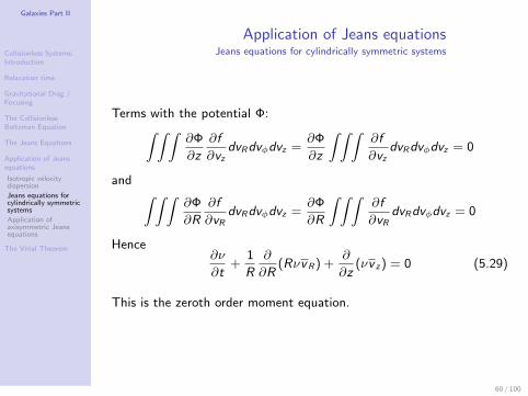
Application of Jeans equationsJeans equations for cylindrically symmetric systems
Terms with the potential Φ:∫ ∫ ∫∂Φ
∂z
∂f
∂vzdvRdvφdvz =
∂Φ
∂z
∫ ∫ ∫∂f
∂vzdvRdvφdvz = 0
and ∫ ∫ ∫∂Φ
∂R
∂f
∂vRdvRdvφdvz =
∂Φ
∂R
∫ ∫ ∫∂f
∂vRdvRdvφdvz = 0
Hence∂ν
∂t+
1
R
∂
∂R(RνvR) +
∂
∂z(νv z) = 0 (5.29)
This is the zeroth order moment equation.
60 / 100

Galaxies Part II
Collisionless Systems:Introduction
Relaxation time
Gravitational Drag /Focusing
The CollisionlessBoltzman Equation
The Jeans Equations
Application of Jeansequations
Isotropic velocitydispersion
Jeans equations forcylindrically symmetricsystems
Application ofaxisymmetric Jeansequations
The Virial Theorem
Application of Jeans equationsJeans equations for cylindrically symmetric systems
There are three first moment equations, corresponding to each of thev components, where we take the collisionless Boltzmann equation×vR , vφ, vz and
∫∫∫dvRdvφdvz .
The results are
∂(νvR)
∂t+∂(νv 2
R)
∂R+∂(νvRvz)
∂z+ ν
(v 2R − v 2
φ
R+∂Φ
∂R
)= 0 (5.30)
∂(νvφ)
∂t+∂(νvRvφ)
∂R+∂(νvφvz)
∂z+
2ν
RvφvR = 0 (5.31)
and
∂(νv z)
∂t+∂(νvRvz)
∂R+∂(νv 2
z )
∂z+νvRvzR
+ ν∂Φ
∂z= 0. (5.32)
Now, this is something powerful.
61 / 100
Galaxies Part II
Collisionless Systems:Introduction
Relaxation time
Gravitational Drag /Focusing
The CollisionlessBoltzman Equation
The Jeans Equations
Application of Jeansequations
Isotropic velocitydispersion
Jeans equations forcylindrically symmetricsystems
Application ofaxisymmetric Jeansequations
The Virial Theorem
Application of Jeans equations
• Spheroidal components with isotropic velocity dispersion
• Asymmetric drift
• Local mass density
• Local velocity ellipsoid
• Mass distribution in the Galaxy out to large radii
62 / 100

Galaxies Part II
Collisionless Systems:Introduction
Relaxation time
Gravitational Drag /Focusing
The CollisionlessBoltzman Equation
The Jeans Equations
Application of Jeansequations
Isotropic velocitydispersion
Jeans equations forcylindrically symmetricsystems
Application ofaxisymmetric Jeansequations
The Virial Theorem
Application of Jeans equationsAsymmetric drift
There is a lag and the lag increases with the age of the stellar tracersand so does the random component of their motion.
63 / 100

Galaxies Part II
Collisionless Systems:Introduction
Relaxation time
Gravitational Drag /Focusing
The CollisionlessBoltzman Equation
The Jeans Equations
Application of Jeansequations
Isotropic velocitydispersion
Jeans equations forcylindrically symmetricsystems
Application ofaxisymmetric Jeansequations
The Virial Theorem
Application of Jeans equationsAsymmetric drift
The distribution of azimuthal velocities vφ = vφ − vc is very skew.This asymmetry arises from two effects.
• Stars near the Sun with vφ < 0 have less angular momentum andthus have Rg < R0 compared to stars with vφ > 0 and Rg > R0.The surface density of stars declines exponentially, hence thereare more stars with smaller Rg .
• The velocity dispersion σR declines with R, so the fraction ofstars with Rg = R0 − δR is larger than the fraction of stars withRg = R0 + δR. Thus there are more stars on eccentric orbits thatcan reach the Sun with vφ < 0
64 / 100

Galaxies Part II
Collisionless Systems:Introduction
Relaxation time
Gravitational Drag /Focusing
The CollisionlessBoltzman Equation
The Jeans Equations
Application of Jeansequations
Isotropic velocitydispersion
Jeans equations forcylindrically symmetricsystems
Application ofaxisymmetric Jeansequations
The Virial Theorem
Application of Jeans equationsAsymmetric drift
The epicyclic approximation:
[vφ − vc(R0)]2
v 2R
' −BA− B
= − B
Ω0=
K 2
4Ω2' 0.5
65 / 100
Galaxies Part II
Collisionless Systems:Introduction
Relaxation time
Gravitational Drag /Focusing
The CollisionlessBoltzman Equation
The Jeans Equations
Application of Jeansequations
Isotropic velocitydispersion
Jeans equations forcylindrically symmetricsystems
Application ofaxisymmetric Jeansequations
The Virial Theorem
Application of Jeans equationsAsymmetric drift
The velocity of the asymmetric drift
va ≡ vc − vφ
Jeans tells us that
∂(νvR)
∂t+∂(νv 2
R)
∂R+∂(νvRvz)
∂z+ ν
(v 2R − v 2
φ
R+∂Φ
∂R
)= 0
We assume
• The Galactic disk is in the steady state
• The Sun lies sufficiently close to the equator, at z = 0
• The disk is symmetric with respect to z and hence ∂ν/∂z = 0
So,
R
ν
∂(νv 2R)
∂R+ R
∂(vRvz)
∂z+ v 2
R − v 2φ + R
∂Φ
∂R= 0 (5.33)
66 / 100
Galaxies Part II
Collisionless Systems:Introduction
Relaxation time
Gravitational Drag /Focusing
The CollisionlessBoltzman Equation
The Jeans Equations
Application of Jeansequations
Isotropic velocitydispersion
Jeans equations forcylindrically symmetricsystems
Application ofaxisymmetric Jeansequations
The Virial Theorem
Application of Jeans equationsAsymmetric drift
R
ν
∂(νv2R
)
∂R+ R ∂(vR vz )
∂z+ v 2
R − v 2φ + R ∂Φ
∂R= 0
Defineσ2φ = v 2
φ − vφ2
Remember that
v 2c = R
∂Φ
∂R
Therefore
σ2φ − v 2
R − R
ν
∂(νv 2R)
∂R− R
∂(vrvz)
∂z= v 2
c − vφ2 (5.34)
= (vc − vφ)(vc + vφ) = va(2vc − va)
If we neglect va compared to 2vc
va 'v 2R
2vc
[σ2φ
v 2R
− 1−∂ ln(νv 2
R)
∂ lnR− R
v 2R
∂(vrvz)
∂z
](5.35)
67 / 100

Galaxies Part II
Collisionless Systems:Introduction
Relaxation time
Gravitational Drag /Focusing
The CollisionlessBoltzman Equation
The Jeans Equations
Application of Jeansequations
Isotropic velocitydispersion
Jeans equations forcylindrically symmetricsystems
Application ofaxisymmetric Jeansequations
The Virial Theorem
Application of Jeans equationsAsymmetric drift
This is Stromberg’s asymmetric drift equation
va 'v 2R
2vc
[σ2φ
v 2R
− 1−∂ ln(νv 2
R)
∂ lnR− R
v 2R
∂(vrvz)
∂z
]
• σ2φ/v
2R = 0.35
• ν and v 2R are both ∝ e−R/Rd with R0/Rd = 3.2
First three terms sum up to 5.8
• The last term is tricky, as it requires measuring the velocityellipsoid outside the plane of the Galaxy, it averages to between 0and -0.8
Averaging over, the value in the brackets is 5.4± 0.4, so
va ' v 2R/(82± 6)kms−1
68 / 100

Galaxies Part II
Collisionless Systems:Introduction
Relaxation time
Gravitational Drag /Focusing
The CollisionlessBoltzman Equation
The Jeans Equations
Application of Jeansequations
Isotropic velocitydispersion
Jeans equations forcylindrically symmetricsystems
Application ofaxisymmetric Jeansequations
The Virial Theorem
Application of Jeans equationsAsymmetric drift
But, what is measured?
69 / 100

Galaxies Part II
Collisionless Systems:Introduction
Relaxation time
Gravitational Drag /Focusing
The CollisionlessBoltzman Equation
The Jeans Equations
Application of Jeansequations
Isotropic velocitydispersion
Jeans equations forcylindrically symmetricsystems
Application ofaxisymmetric Jeansequations
The Virial Theorem
Application of Jeans equationsAsymmetric drift
70 / 100

Galaxies Part II
Collisionless Systems:Introduction
Relaxation time
Gravitational Drag /Focusing
The CollisionlessBoltzman Equation
The Jeans Equations
Application of Jeansequations
Isotropic velocitydispersion
Jeans equations forcylindrically symmetricsystems
Application ofaxisymmetric Jeansequations
The Virial Theorem
Application of Jeans equationsAsymmetric drift
Something has been heating the disk! Curious what that might be.
• Heating by MACHOs
• Scattering of disk stars by molecular clouds
• Scattering by spiral arms
71 / 100

Galaxies Part II
Collisionless Systems:Introduction
Relaxation time
Gravitational Drag /Focusing
The CollisionlessBoltzman Equation
The Jeans Equations
Application of Jeansequations
Isotropic velocitydispersion
Jeans equations forcylindrically symmetricsystems
Application ofaxisymmetric Jeansequations
The Virial Theorem
Application of Jeans equationsAsymmetric drift
...MACHOs???
MACHO = MAssive Compact Halo Object.
This was the primary candidate for the baryonic Dark Matter(as considered only 10-15 years ago).
Anything dark, massive and not fuzzy goes:
• black holes
• neutron stars
• very old white dwarfs = black dwarfs?
• brown dwarfs
• rogue planets
72 / 100

Galaxies Part II
Collisionless Systems:Introduction
Relaxation time
Gravitational Drag /Focusing
The CollisionlessBoltzman Equation
The Jeans Equations
Application of Jeansequations
Isotropic velocitydispersion
Jeans equations forcylindrically symmetricsystems
Application ofaxisymmetric Jeansequations
The Virial Theorem
Application of Jeans equationsAsymmetric drift
Unfortunately, any significant contribution of MACHOs to theGalaxy’s mass budget is ruled out, due to
• they are too efficient in heating the disk and predict theamplitude of the effect to grow faster with time than observed
• can be detected directly through observations of gravitationalmicrolensing effect. While the first claims put fMACHO ∼ 20%, itis consistent with zero.
73 / 100

Galaxies Part II
Collisionless Systems:Introduction
Relaxation time
Gravitational Drag /Focusing
The CollisionlessBoltzman Equation
The Jeans Equations
Application of Jeansequations
Isotropic velocitydispersion
Jeans equations forcylindrically symmetricsystems
Application ofaxisymmetric Jeansequations
The Virial Theorem
Application of Jeans equationsAsymmetric drift
We know that the irregularities in the Galaxy’s gravitational potentialheat the disk and (re)shape the velocity distribution of the disk stars.
We do not know exactly which phenomenon is the primary source ofheating
Most likely, it is the combined effects of spiral transients andmolecular clouds
74 / 100

Galaxies Part II
Collisionless Systems:Introduction
Relaxation time
Gravitational Drag /Focusing
The CollisionlessBoltzman Equation
The Jeans Equations
Application of Jeansequations
Isotropic velocitydispersion
Jeans equations forcylindrically symmetricsystems
Application ofaxisymmetric Jeansequations
The Virial Theorem
Application of Jeans equationsAsymmetric drift
We predicted va ' v 2R/(82± 6)kms−1
The measured value from above:
va = v 2R/(80± 5)kms−1
75 / 100

Galaxies Part II
Collisionless Systems:Introduction
Relaxation time
Gravitational Drag /Focusing
The CollisionlessBoltzman Equation
The Jeans Equations
Application of Jeansequations
Isotropic velocitydispersion
Jeans equations forcylindrically symmetricsystems
Application ofaxisymmetric Jeansequations
The Virial Theorem
Application of Jeans equationsLocal mass density
The mass density in the solar neighborhood.Equation (5.32) can be written as
∂(νv z)
∂t+
1
R
∂(RνvRvz)
∂R+∂(νv 2
z )
∂z+ ν
∂Φ
∂z= 0
Take this equation and assume a steady state so ∂∂t
= 0, so have
1
R
∂(RνvRvz)
∂R+∂(νv 2
z )
∂z= −ν ∂Φ
∂z
76 / 100

Galaxies Part II
Collisionless Systems:Introduction
Relaxation time
Gravitational Drag /Focusing
The CollisionlessBoltzman Equation
The Jeans Equations
Application of Jeansequations
Isotropic velocitydispersion
Jeans equations forcylindrically symmetricsystems
Application ofaxisymmetric Jeansequations
The Virial Theorem
Application of Jeans equationsLocal mass density
We are interested in the density in a thin disk, where the density fallsoff much faster in z than in R. Typically disk a few 100pc thick, witha radial scale of a few kpc, so
∂
∂z∼ 10
∂
∂R∼ 10
1
R
so neglect ∂∂R
term. So
1
ν
∂
∂z(νv 2
z ) = −∂Φ
∂z
i.e.vertical pressure balances vertical gravity. This is the Jeansequation for one-dimensional slab.Also can show that Poisson’s equation in a thin disk approximation is
∂2Φ
∂z2= 4πGρ
where ρ is the total mass density.So have
∂
∂z
1
ν
∂
∂z(νv 2
z ) = −4πGρ.
77 / 100

Galaxies Part II
Collisionless Systems:Introduction
Relaxation time
Gravitational Drag /Focusing
The CollisionlessBoltzman Equation
The Jeans Equations
Application of Jeansequations
Isotropic velocitydispersion
Jeans equations forcylindrically symmetricsystems
Application ofaxisymmetric Jeansequations
The Virial Theorem
Application of Jeans equationsLocal mass density
Note that by f we do not necessarily mean all stars, it could be anywell-defined subset, such as all G stars (say).
The ν is the number density of G stars or whatever type is chosen. Wehave not linked ν and Φ (or ν and ρ) as was done in the previousexample of a self-consistent spherical model.
Thus if for any population of stars we can measure v 2z and ν as a
function of height z we can calculate the total local density ρ. Thisinvolves differentiation of really noisy data, so the results are veryuncertain.Using this technique for F stars + K giants Oort found
ρ0 = ρ(R0, z = 0) = 0.15 M pc−3= Oort limit.
78 / 100

Galaxies Part II
Collisionless Systems:Introduction
Relaxation time
Gravitational Drag /Focusing
The CollisionlessBoltzman Equation
The Jeans Equations
Application of Jeansequations
Isotropic velocitydispersion
Jeans equations forcylindrically symmetricsystems
Application ofaxisymmetric Jeansequations
The Virial Theorem
Application of Jeans equationsLocal mass density
Note that one can determine instead
Σ(z) =
∫ z
−z
ρdz ′ = − 1
2πGν
∂
∂z(νv 2
z )
more accurately (since there is one less difference, or differential,involved).
Oort: Σ(700pc) ' 90 M pc−2
This compares with the observable mass:Σ(1.1kpc) ' 71± 6 M pc−2 (Kuijken & Gilmore, 1991)
The baryons account for Σ(stars plus gas) ' 41± 15 M pc−2
(Binney & Evans, 2001)
79 / 100

Galaxies Part II
Collisionless Systems:Introduction
Relaxation time
Gravitational Drag /Focusing
The CollisionlessBoltzman Equation
The Jeans Equations
Application of Jeansequations
Isotropic velocitydispersion
Jeans equations forcylindrically symmetricsystems
Application ofaxisymmetric Jeansequations
The Virial Theorem
Application of Jeans equationsLocal mass density
Or we can estimate Dark Matter halo’s contribution to Σ bysupposing that
• the halo is spherical
• the circular speed vc = v0 = constant
• without the halo, vc = (GMd/r)1/2
Then, the halo mass M(r) satisfies G [M(r) + Md ] = rv 20
The halo’s density:
ρh =1
4πr 2
dM
dr=
v 20
4πGr 2= 0.014Mpc
−3
(v0
200kms−1
)2(R0
8kpc
)−2
The halo’s contribution Σh1.1 = 2.2 kpc× ρh = 30.6Mpc
−2
So local dark matter is relatively tightly constrained, and the Sun liesin transition region in which both disk and halo contribute significantmasses.
80 / 100

Galaxies Part II
Collisionless Systems:Introduction
Relaxation time
Gravitational Drag /Focusing
The CollisionlessBoltzman Equation
The Jeans Equations
Application of Jeansequations
Isotropic velocitydispersion
Jeans equations forcylindrically symmetricsystems
Application ofaxisymmetric Jeansequations
The Virial Theorem
Application of Jeans equationsMass profile of the Galaxy
Jeans equation for spherical systems:
d(νv 2r )
dr+ ν
(dΦ
dr+
2v 2r − v 2
θ − v 2φ
r
)= 0 (5.36)
For the stationary and spherically symmetric Galactic halo, the radialvelocity dispersion σr,∗ of stars with density ρ∗ obeys the above Jeansequation (albeit modified slightly):
1
ρ∗
d(ρ∗σ2r,∗)
dr+
2βσ2r,∗
r= −dΦ
dr= −v 2
c
r(5.37)
where the velocity anisotropy parameter is
β ≡ 1−σ2θ + σ2
φ
2σ2r
= 1−v 2θ + v 2
φ
2v 2r
(5.38)
Thus, the Jeans equation allows us to determine a unique solution forthe mass profile if we know σ2
r,∗, ρ∗ and β(r).
81 / 100
Galaxies Part II
Collisionless Systems:Introduction
Relaxation time
Gravitational Drag /Focusing
The CollisionlessBoltzman Equation
The Jeans Equations
Application of Jeansequations
Isotropic velocitydispersion
Jeans equations forcylindrically symmetricsystems
Application ofaxisymmetric Jeansequations
The Virial Theorem
Application of Jeans equationsMass profile of the Galaxy
The expected radial velocity dispersion for a tracer population isderived by integrating the Jeans equation:
σ2r,∗ =
1
ρ∗e∫
2βdx
∫ ∞x
ρ∗v2c e
∫2βdx
′′
dx′, x = ln r (5.39)
However, the proper motions are not available for the majority of thetracers, therefore we can only measure the line-of-sight velocitydispersion:
σGSR,∗(r) = σr,∗(r)√
1− βH(r) (5.40)
Where
H(r) =r 2 + R2
4r 2− (r 2 − R2
)2
8r 3Rln
r + Rr − R
(5.41)
82 / 100

Galaxies Part II
Collisionless Systems:Introduction
Relaxation time
Gravitational Drag /Focusing
The CollisionlessBoltzman Equation
The Jeans Equations
Application of Jeansequations
Isotropic velocitydispersion
Jeans equations forcylindrically symmetricsystems
Application ofaxisymmetric Jeansequations
The Virial Theorem
Application of Jeans equationsMass profile of the Galaxy
Alternatively,
M(r) = − rσ2r
G
[d ln ν
d ln r+
d lnσ2r
d ln r+ 2β(r)
](5.42)
83 / 100

Galaxies Part II
Collisionless Systems:Introduction
Relaxation time
Gravitational Drag /Focusing
The CollisionlessBoltzman Equation
The Jeans Equations
Application of Jeansequations
Isotropic velocitydispersion
Jeans equations forcylindrically symmetricsystems
Application ofaxisymmetric Jeansequations
The Virial Theorem
Application of Jeans equationsMass profile of the Galaxy
Still, there are further complications. Namely, the two ingredients areuncertain
• the behavior of the stellar velocity anisotropy
• stellar halo density profile at large radii
84 / 100

Galaxies Part II
Collisionless Systems:Introduction
Relaxation time
Gravitational Drag /Focusing
The CollisionlessBoltzman Equation
The Jeans Equations
Application of Jeansequations
Isotropic velocitydispersion
Jeans equations forcylindrically symmetricsystems
Application ofaxisymmetric Jeansequations
The Virial Theorem
Application of Jeans equationsMass profile of the Galaxy
from Battaglia et al, 2005
85 / 100

Galaxies Part II
Collisionless Systems:Introduction
Relaxation time
Gravitational Drag /Focusing
The CollisionlessBoltzman Equation
The Jeans Equations
Application of Jeansequations
Isotropic velocitydispersion
Jeans equations forcylindrically symmetricsystems
Application ofaxisymmetric Jeansequations
The Virial Theorem
Application of Jeans equationsMass profile of the Galaxy
With constant velocity anisotropy
86 / 100
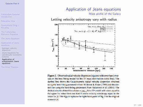
Galaxies Part II
Collisionless Systems:Introduction
Relaxation time
Gravitational Drag /Focusing
The CollisionlessBoltzman Equation
The Jeans Equations
Application of Jeansequations
Isotropic velocitydispersion
Jeans equations forcylindrically symmetricsystems
Application ofaxisymmetric Jeansequations
The Virial Theorem
Application of Jeans equationsMass profile of the Galaxy
Letting velocity anisotropy vary with radius
87 / 100

Galaxies Part II
Collisionless Systems:Introduction
Relaxation time
Gravitational Drag /Focusing
The CollisionlessBoltzman Equation
The Jeans Equations
Application of Jeansequations
The Virial Theorem
Potential-energy tensor
Kinetic-energy tensor
Tensor Virial Theorem
Scalar Virial Theorem
Applications VirialTheorem
The Virial Theorem
We have obtained the first moment of CBE by multiplying it throughby vj and integrating over all velocities. This allowed us to reduce anequation for 6D distribution function f to an equation for 3D densityν and the velocity moments:
∂
∂t(νv j) +
∂
∂xi(νvivj) + ν
∂Φ
∂xj= 0 (5.43)
Now, let us multiply the above equation ↑ by xk and integrate over allpositions, converting these differential 1st moment equations into atensor equation relating the global properties of the galaxy such askinetic energy.∫
d3xxk∂(ρv j)
∂t= −
∫d3xxk
∂(ρvivj)
∂xi−∫
d3xρxk∂Φ
∂xj(5.44)
88 / 100

Galaxies Part II
Collisionless Systems:Introduction
Relaxation time
Gravitational Drag /Focusing
The CollisionlessBoltzman Equation
The Jeans Equations
Application of Jeansequations
The Virial Theorem
Potential-energy tensor
Kinetic-energy tensor
Tensor Virial Theorem
Scalar Virial Theorem
Applications VirialTheorem
The Virial TheoremPotential-energy tensor
∫
d3xxk∂(ρv j )
∂t= −
∫d3xxk
∂(ρvi vj )
∂xi−∫d3xρxk
∂Φ∂xj
By definition, the Chandrasekhar potential-energy tensor:
Wjk ≡ −∫
d3xρ(x)xj∂Φ
∂xk(5.45)
Also, by definition:
Φ(x) ≡ −G∫
d3x′ ρ(x
′)
|x′ − x|(5.46)
Which makes W on substituting Φ:
Wjk = G
∫d3xρ(x)xj
∂
∂xk
∫d3x
′ ρ(x′)
|x′ − x|(5.47)
89 / 100

Galaxies Part II
Collisionless Systems:Introduction
Relaxation time
Gravitational Drag /Focusing
The CollisionlessBoltzman Equation
The Jeans Equations
Application of Jeansequations
The Virial Theorem
Potential-energy tensor
Kinetic-energy tensor
Tensor Virial Theorem
Scalar Virial Theorem
Applications VirialTheorem
The Virial TheoremPotential-energy tensor
∫
d3xxk∂(ρv j )
∂t= −
∫d3xxk
∂(ρvi vj )
∂xi−∫d3xρxk
∂Φ∂xj
Taking the differentiation inside the integral, re-labeling the dummyvariables x and x
′and writing Wjk twice, we get:
Wjk = −1
2G
∫d3x
∫d3x
′ρ(x)ρ(x
′)
(x′j − xj)(x
′k − xk)
|x′ − x|3(5.48)
Therefore, W is symmetric, i.e. Wjk = Wkj . Taking the trace:
trace(W) ≡3∑
j=1
Wjj = −1
2G
∫d3x ρ(x)
∫d3x
′ ρ(x′)
|x′ − x|
=1
2
∫d3x ρ(x) Φ(x)
(5.49)
This is the total potential energy of the body W ,
W = −∫
d3x ρ x∇Φ. (5.50)
90 / 100
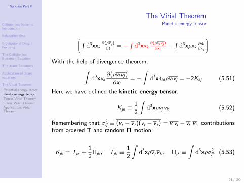
Galaxies Part II
Collisionless Systems:Introduction
Relaxation time
Gravitational Drag /Focusing
The CollisionlessBoltzman Equation
The Jeans Equations
Application of Jeansequations
The Virial Theorem
Potential-energy tensor
Kinetic-energy tensor
Tensor Virial Theorem
Scalar Virial Theorem
Applications VirialTheorem
The Virial TheoremKinetic-energy tensor
∫
d3xxk∂(ρv j )
∂t= −
∫d3xxk
∂(ρvi vj )
∂xi−∫d3xρxk
∂Φ∂xj
With the help of divergence theorem:∫d3xxk
∂(ρvivj)
∂xi= −
∫d3xδkiρvivj = −2Kkj (5.51)
Here we have defined the kinetic-energy tensor:
Kjk ≡1
2
∫d3xρvjvk (5.52)
Remembering that σ2ij ≡ (vi − v i )(vj − v j) = vivj − vi vj , contributions
from ordered T and random Π motion:
Kjk = Tjk +1
2Πjk , Tjk ≡
1
2
∫d3xρv jv k , Πjk ≡
∫d3xρσ2
jk (5.53)
91 / 100
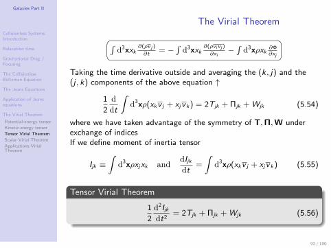
Galaxies Part II
Collisionless Systems:Introduction
Relaxation time
Gravitational Drag /Focusing
The CollisionlessBoltzman Equation
The Jeans Equations
Application of Jeansequations
The Virial Theorem
Potential-energy tensor
Kinetic-energy tensor
Tensor Virial Theorem
Scalar Virial Theorem
Applications VirialTheorem
The Virial Theorem
∫
d3xxk∂(ρv j )
∂t= −
∫d3xxk
∂(ρvi vj )
∂xi−∫d3xρxk
∂Φ∂xj
Taking the time derivative outside and averaging the (k, j) and the(j , k) components of the above equation ↑
1
2
d
dt
∫d3xρ(xkv j + xjv k) = 2Tjk + Πjk + Wjk (5.54)
where we have taken advantage of the symmetry of T,Π,W underexchange of indicesIf we define moment of inertia tensor
Ijk ≡∫
d3xρxjxk anddIjkdt
=
∫d3xρ(xkv j + xjv k) (5.55)
Tensor Virial Theorem
1
2
d2Ijkdt2
= 2Tjk + Πjk + Wjk (5.56)
92 / 100

Galaxies Part II
Collisionless Systems:Introduction
Relaxation time
Gravitational Drag /Focusing
The CollisionlessBoltzman Equation
The Jeans Equations
Application of Jeansequations
The Virial Theorem
Potential-energy tensor
Kinetic-energy tensor
Tensor Virial Theorem
Scalar Virial Theorem
Applications VirialTheorem
The Virial Theorem
• The theorem is derived for collisionless systems, but can beproven for self-gravitating collisional systems too.
• This is the equation of energy balance in systems in equilibriumunder gravity.
• Can be extended to include energy from turbulence andconvective motions, magnetic energy etc
1
2
d2Ijkdt2 = 2Tjk + Πjk + Wjk
In a steady state I = 0, the trace of the Tensor Virial Theoremequation above is:
Scalar Virial Theorem
2K + W = 0 (5.57)
where
K ≡ trace(T) +1
2trace(Π) (5.58)
93 / 100

Galaxies Part II
Collisionless Systems:Introduction
Relaxation time
Gravitational Drag /Focusing
The CollisionlessBoltzman Equation
The Jeans Equations
Application of Jeansequations
The Virial Theorem
Potential-energy tensor
Kinetic-energy tensor
Tensor Virial Theorem
Scalar Virial Theorem
Applications VirialTheorem
The Virial Theorem
Curiously, if E is the energy of the system then
E = K + W = −K =1
2W (5.59)
94 / 100
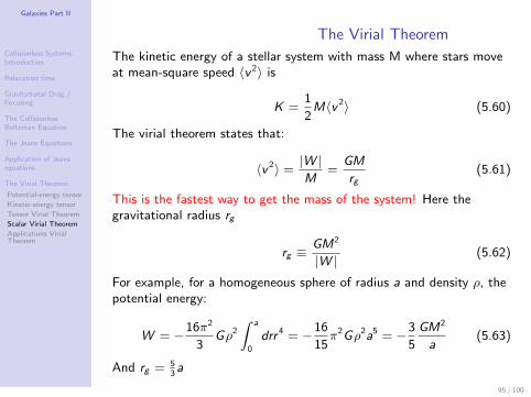
Galaxies Part II
Collisionless Systems:Introduction
Relaxation time
Gravitational Drag /Focusing
The CollisionlessBoltzman Equation
The Jeans Equations
Application of Jeansequations
The Virial Theorem
Potential-energy tensor
Kinetic-energy tensor
Tensor Virial Theorem
Scalar Virial Theorem
Applications VirialTheorem
The Virial Theorem
The kinetic energy of a stellar system with mass M where stars moveat mean-square speed 〈v 2〉 is
K =1
2M〈v 2〉 (5.60)
The virial theorem states that:
〈v 2〉 =|W |M
=GM
rg(5.61)
This is the fastest way to get the mass of the system! Here thegravitational radius rg
rg ≡GM2
|W | (5.62)
For example, for a homogeneous sphere of radius a and density ρ, thepotential energy:
W = −16π2
3Gρ2
∫ a
0
drr 4 = −16
15π2Gρ2a5 = −3
5
GM2
a(5.63)
And rg = 53a
95 / 100
Galaxies Part II
Collisionless Systems:Introduction
Relaxation time
Gravitational Drag /Focusing
The CollisionlessBoltzman Equation
The Jeans Equations
Application of Jeansequations
The Virial Theorem
Potential-energy tensor
Kinetic-energy tensor
Tensor Virial Theorem
Scalar Virial Theorem
Applications VirialTheorem
The Virial TheoremApplications Virial Theorem
• Despite the elegance of the Virial Theorem, its applications arenot straightforward.
• This is because neither 〈v 2〉 or rg are readily available for mostsystems.
• Instead of 〈v 2〉, the line of sight velocity dispersion 〈v 2‖〉 is used.
• And isotropy is assumed (not going to work in many situations)
〈v 2〉 = 3〈v 2‖〉
• Instead of gravitational radius rg the rough extent of the systemis used
• or use the so-called half-mass radius rh obtained by integratinglight and assuming mass/light ratio. It can be shown that forvariety of systems rh/rg ∼ 1
2
See Eddington (1916). Einstein (1921) used the Virial Theorem toestimate the mass of globular clusters.
96 / 100
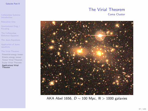
Galaxies Part II
Collisionless Systems:Introduction
Relaxation time
Gravitational Drag /Focusing
The CollisionlessBoltzman Equation
The Jeans Equations
Application of Jeansequations
The Virial Theorem
Potential-energy tensor
Kinetic-energy tensor
Tensor Virial Theorem
Scalar Virial Theorem
Applications VirialTheorem
The Virial TheoremComa Cluster
AKA Abel 1656, D ∼ 100 Mpc, N > 1000 galaxies
97 / 100

Galaxies Part II
Collisionless Systems:Introduction
Relaxation time
Gravitational Drag /Focusing
The CollisionlessBoltzman Equation
The Jeans Equations
Application of Jeansequations
The Virial Theorem
Potential-energy tensor
Kinetic-energy tensor
Tensor Virial Theorem
Scalar Virial Theorem
Applications VirialTheorem
The Virial TheoremFritz Zwicky and the Coma Cluster
98 / 100
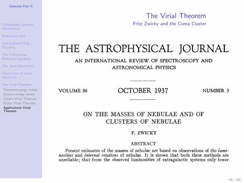
Galaxies Part II
Collisionless Systems:Introduction
Relaxation time
Gravitational Drag /Focusing
The CollisionlessBoltzman Equation
The Jeans Equations
Application of Jeansequations
The Virial Theorem
Potential-energy tensor
Kinetic-energy tensor
Tensor Virial Theorem
Scalar Virial Theorem
Applications VirialTheorem
The Virial TheoremFritz Zwicky and the Coma Cluster
99 / 100

Galaxies Part II
Collisionless Systems:Introduction
Relaxation time
Gravitational Drag /Focusing
The CollisionlessBoltzman Equation
The Jeans Equations
Application of Jeansequations
The Virial Theorem
Potential-energy tensor
Kinetic-energy tensor
Tensor Virial Theorem
Scalar Virial Theorem
Applications VirialTheorem
The Virial TheoremFritz Zwicky and the Coma Cluster
100 / 100

Galaxies Part II
Collisionless Systems:Introduction
Relaxation time
Gravitational Drag /Focusing
The CollisionlessBoltzman Equation
The Jeans Equations
Application of Jeansequations
The Virial Theorem
Potential-energy tensor
Kinetic-energy tensor
Tensor Virial Theorem
Scalar Virial Theorem
Applications VirialTheorem
The Virial TheoremFritz Zwicky and the Coma Cluster
101 / 100