8

Chapter 2

THE ZPL APPROACH

ZPL is a parallel programming language developed at the University of Washington.

Designed from first principles, it is unique in providing a mostly p-independent semantics

alongside syntactically identifiable communication. This chapter presents a brief introduc-

tion to ZPL and provides a basis for the extensions described in later chapters; For more

information on ZPL, the reader is referred to the literature [AGNS90, AGL+98, AS91,

CCL+96, CCS97, CCL+98a, CLS98, CCL+98b, CLS99a, CLS99b, CDS00, CCL+00, CS01,

Cha01, CCDS04, CS97, Cho99, CD02, DCS01, DCS02, DCCS03, Dei03, DCS04, DLMW95,

GHNS90, LLST95, LLS98, LS00, Lew01, LS90, LS91, Lin92, LW93, LS93, LS94a, LS94b,

LSA+95, NS92, NSC97, Ngo97, RBS96, Sny86, Sny94, Sny95, Sny99, Sny01, Wea99].

Throughout this chapter, changes to ZPL from the literature will be noted. In addition,

how the current implementation differs from the features described will be noted. Lastly, it

will be noted periodically that the base of ZPL is mostly p-independent.

2.1 ZPL’s Parallel Programming Model

ZPL holds to a simple parallel programming model in which data is either replicated or

distributed. In both cases, there is logically one copy of any given data object; replicated

data is kept consistent via an implicit consistency guarantee brought to fruition by an array

of static typechecking rules.

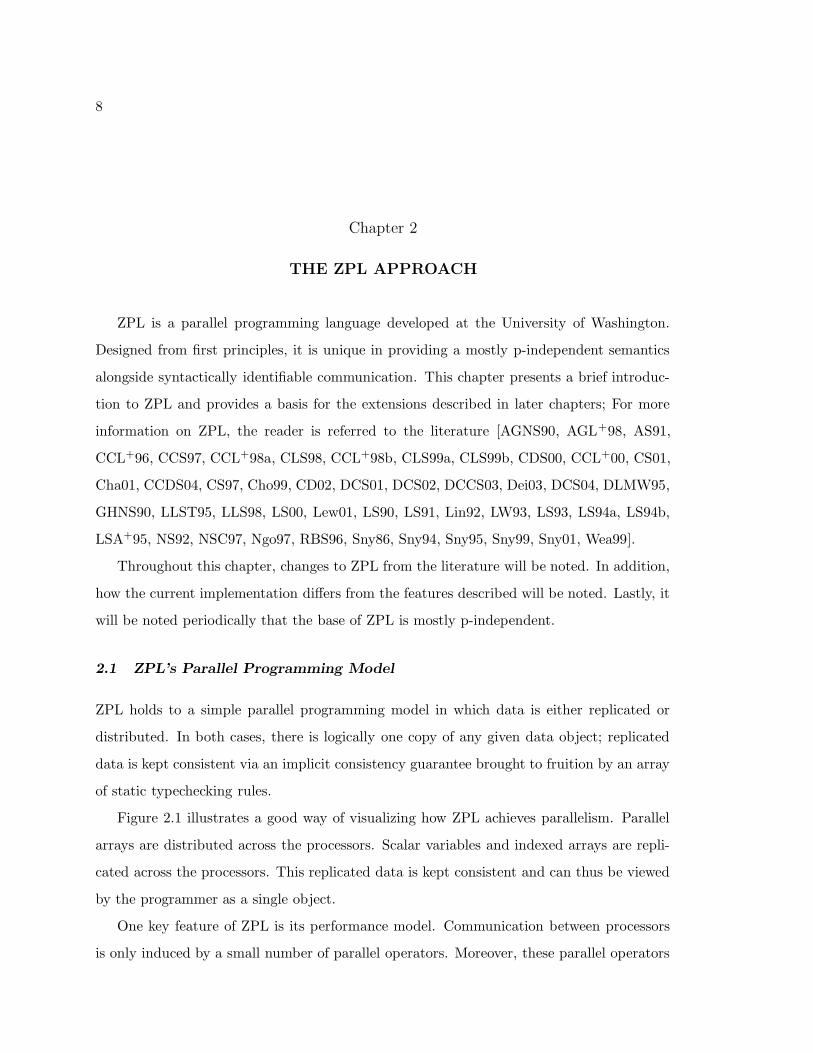
Figure 2.1 illustrates a good way of visualizing how ZPL achieves parallelism. Parallel

arrays are distributed across the processors. Scalar variables and indexed arrays are repli-

cated across the processors. This replicated data is kept consistent and can thus be viewed

by the programmer as a single object.

One key feature of ZPL is its performance model. Communication between processors

is only induced by a small number of parallel operators. Moreover, these parallel operators

9

Figure 2.1: An Illustration of ZPL’s Parallel Programming Model

LocaleP

Locale1

Locale0

...

...

...

...Indexed Arrays

Variables

Parallel Arrays

signal the kind of communication that may take place.

Unlike most SPMD programming languages, most of ZPL is p-independent. This makes

ZPL fundamentally different from languages like UPC and Titanium in which synchroniza-

tion poses a serious challenge to the programmer. In ZPL, synchronization is implicit in

the programming model. Race conditions and deadlocks are impossible.

2.2 Scalar Constructs

ZPL’s parallelism stems from regions and parallel arrays, introduced in Section 2.3. This

section presents ZPL’s scalar constructs. They mimic Modula-2 [Wir83] and are described

only briefly.

2.2.1 Types, Constants, and Variables

ZPL provides standard support for types, constants, and variables. In the parallel imple-

mentation, types and constants are replicated across the processors. Because they contain

the same value on each processor, there is logically one of each type and constant. Variables

are also replicated across the processors. By replicating the serial computation across the

processor set as well, the replicated variables are kept consistent and can be thought of as

10

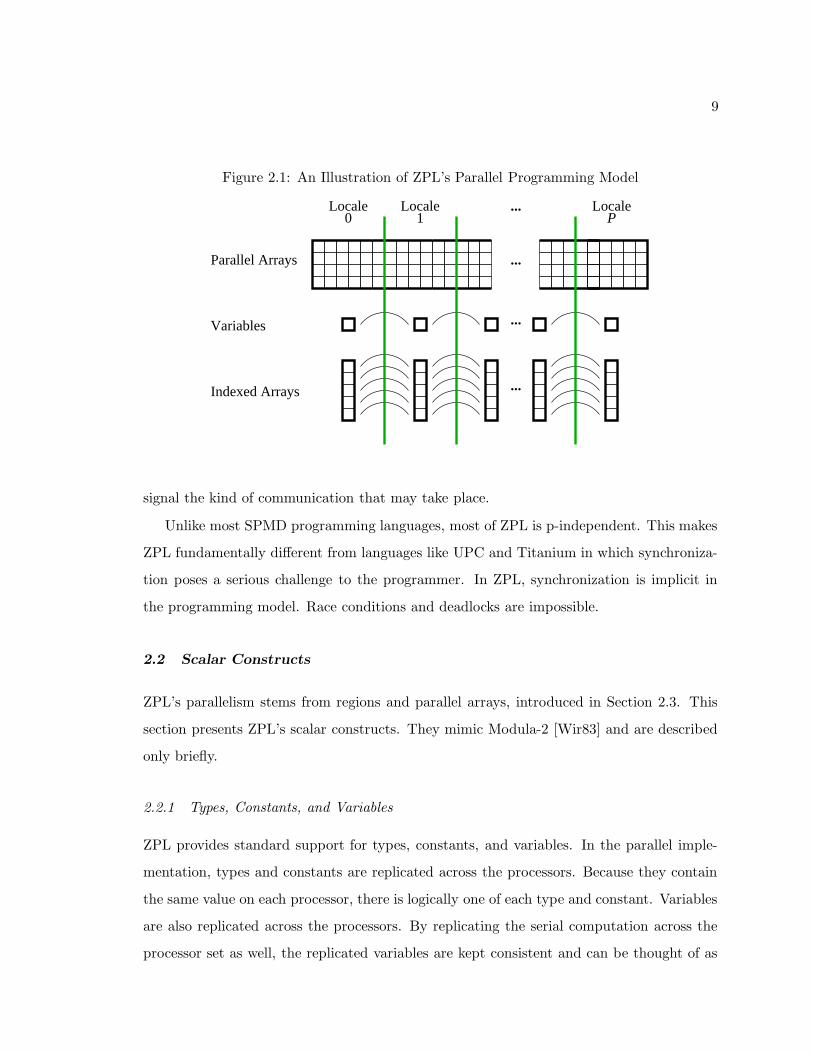
Figure 2.2: Type Coercion of a Selection of ZPL’s Scalar Types

char

string

float

complexdouble

dcomplex

integer

boolean

being a singular value.

2.2.2 Scalar Type Coercion

ZPL is a strongly typed language that supports type coercion on its base types. This is an

important aspect to ZPL’s base types that, as will be seen, extends to its parallel types as

well. Figure 2.2 illustrates the implicit type coercions of ZPL. Expressions of a type lower

in the hierarchy are automatically converted to expressions of a type higher in the hierarchy

where necessary. Thus if a double value and an integer value are added together, the

result is a double value. ZPL also supports explicit type coercions on most of the base

types using a set of standard functions, e.g., to_integer.

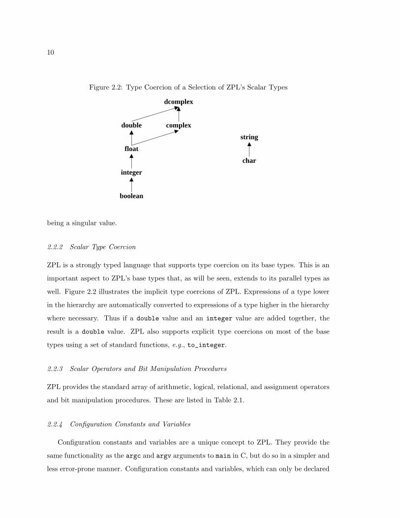
2.2.3 Scalar Operators and Bit Manipulation Procedures

ZPL provides the standard array of arithmetic, logical, relational, and assignment operators

and bit manipulation procedures. These are listed in Table 2.1.

2.2.4 Configuration Constants and Variables

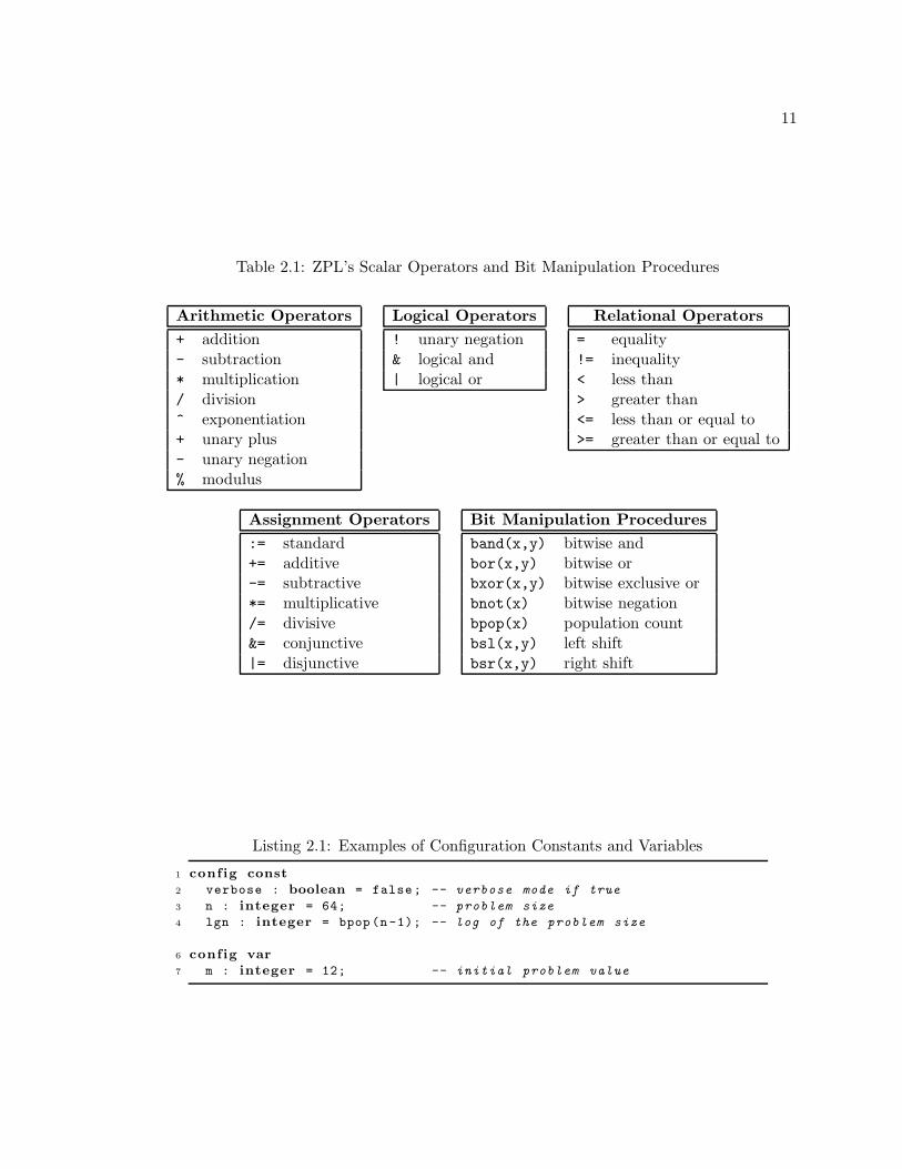
Configuration constants and variables are a unique concept to ZPL. They provide the

same functionality as the argc and argv arguments to main in C, but do so in a simpler and

less error-prone manner. Configuration constants and variables, which can only be declared

11

Table 2.1: ZPL’s Scalar Operators and Bit Manipulation Procedures

Arithmetic Operators

+ addition- subtraction* multiplication/ division^ exponentiation+ unary plus- unary negation% modulus

Logical Operators

! unary negation& logical and| logical or

Relational Operators

= equality!= inequality< less than> greater than<= less than or equal to>= greater than or equal to

Assignment Operators

:= standard+= additive-= subtractive*= multiplicative/= divisive&= conjunctive|= disjunctive

Bit Manipulation Procedures

band(x,y) bitwise andbor(x,y) bitwise orbxor(x,y) bitwise exclusive orbnot(x) bitwise negationbpop(x) population countbsl(x,y) left shiftbsr(x,y) right shift

Listing 2.1: Examples of Configuration Constants and Variables

1 config const

2 verbose : boolean = false; -- verbose mode if true

3 n : integer = 64; -- problem size

4 lgn : integer = bpop (n -1); -- log of the problem size

6 config var

7 m : integer = 12; -- initial problem value

12

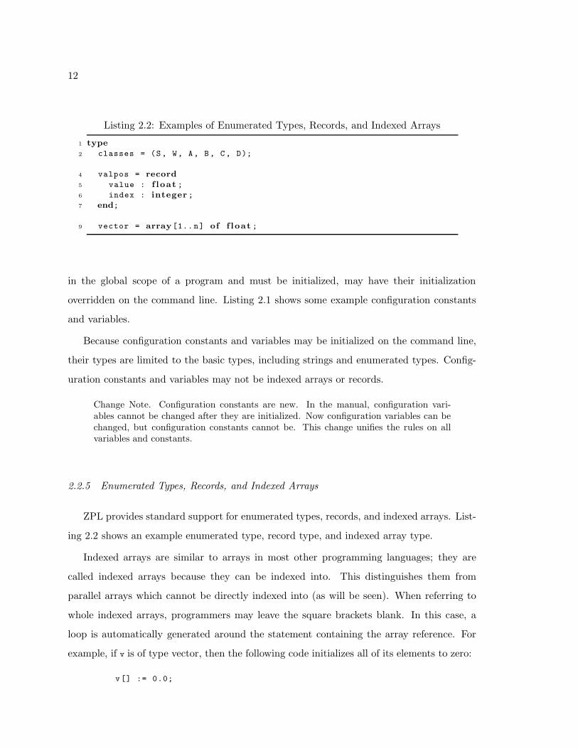
Listing 2.2: Examples of Enumerated Types, Records, and Indexed Arrays

1 type

2 classes = (S, W, A, B, C, D);

4 valpos = record

5 value : f loat ;

6 index : integer ;

7 end;

9 vector = array[1.. n] of f loat ;

in the global scope of a program and must be initialized, may have their initialization

overridden on the command line. Listing 2.1 shows some example configuration constants

and variables.

Because configuration constants and variables may be initialized on the command line,

their types are limited to the basic types, including strings and enumerated types. Config-

uration constants and variables may not be indexed arrays or records.

Change Note. Configuration constants are new. In the manual, configuration vari-ables cannot be changed after they are initialized. Now configuration variables can bechanged, but configuration constants cannot be. This change unifies the rules on allvariables and constants.

2.2.5 Enumerated Types, Records, and Indexed Arrays

ZPL provides standard support for enumerated types, records, and indexed arrays. List-

ing 2.2 shows an example enumerated type, record type, and indexed array type.

Indexed arrays are similar to arrays in most other programming languages; they are

called indexed arrays because they can be indexed into. This distinguishes them from

parallel arrays which cannot be directly indexed into (as will be seen). When referring to

whole indexed arrays, programmers may leave the square brackets blank. In this case, a

loop is automatically generated around the statement containing the array reference. For

example, if v is of type vector, then the following code initializes all of its elements to zero:

v[] := 0.0;

13

In a statement, multiple blank array references must conform, i.e., the blank dimensions

must be the same size and shape.

Counterintuitively, indexed arrays are considered scalars in ZPL. This further distin-

guishes them from parallel arrays.

2.2.6 Input/Output

Basic input and output is handled in ZPL by three procedures, write, writeln, and read.

The write procedure writes its arguments in the order that they are specified. The writeln

procedure behaves identically except that a linefeed follows its last argument. The read

procedure reads its arguments in the order that they are specified.

ZPL also provides a halt procedure to end a program’s execution. The halt procedure

behaves just like the writeln procedure except that the program is terminated after it

completes.

2.2.7 Control Flow and Procedures

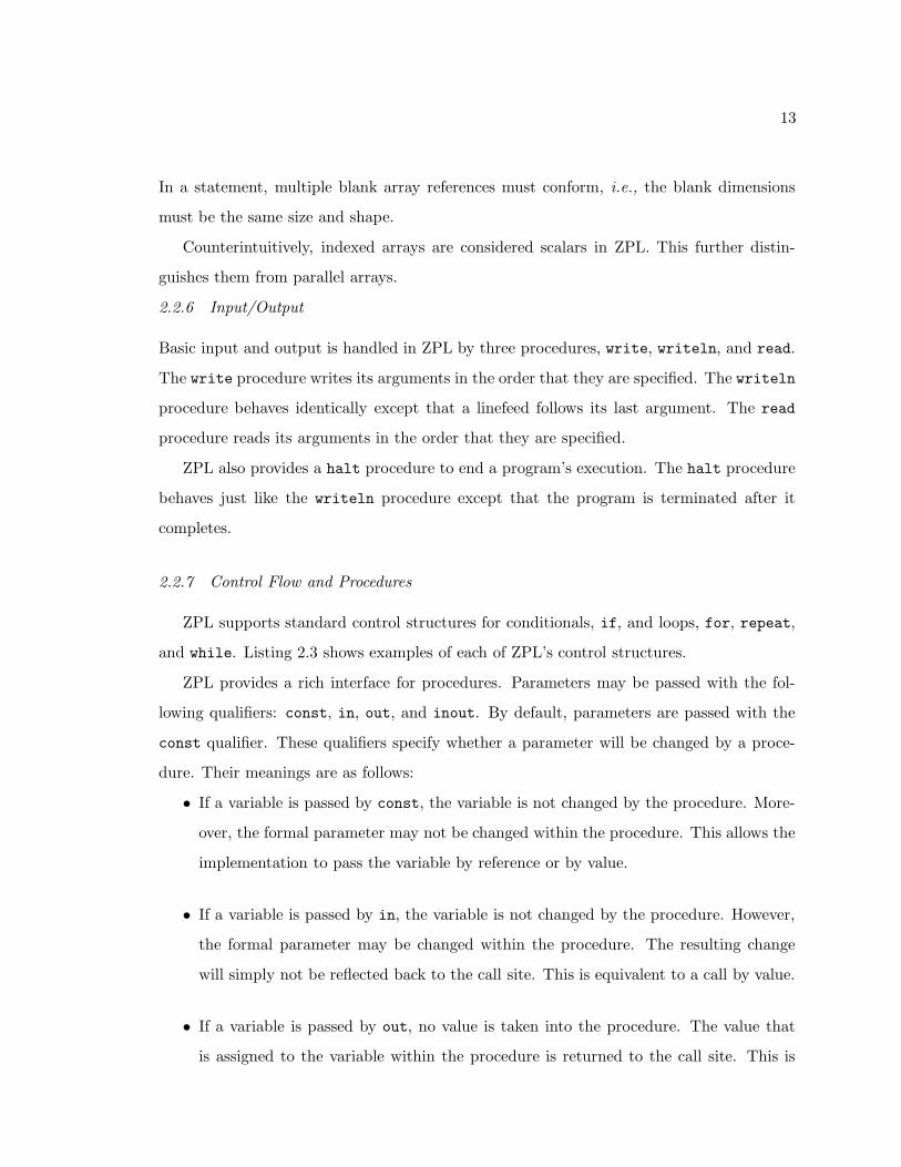
ZPL supports standard control structures for conditionals, if, and loops, for, repeat,

and while. Listing 2.3 shows examples of each of ZPL’s control structures.

ZPL provides a rich interface for procedures. Parameters may be passed with the fol-

lowing qualifiers: const, in, out, and inout. By default, parameters are passed with the

const qualifier. These qualifiers specify whether a parameter will be changed by a proce-

dure. Their meanings are as follows:

• If a variable is passed by const, the variable is not changed by the procedure. More-

over, the formal parameter may not be changed within the procedure. This allows the

implementation to pass the variable by reference or by value.

• If a variable is passed by in, the variable is not changed by the procedure. However,

the formal parameter may be changed within the procedure. The resulting change

will simply not be reflected back to the call site. This is equivalent to a call by value.

• If a variable is passed by out, no value is taken into the procedure. The value that

is assigned to the variable within the procedure is returned to the call site. This is

14

Listing 2.3: Examples of Enumerated Types, Records, and Indexed Arrays

1 i f n <= 0 then

2 halt ("Problem size is too small.");

3 e l s i f bpop(n) != 1 then

4 halt ("Problem size is not a power of two.");

5 e lse

6 writeln("Problem size = " , n);

7 end;

9 for i := 1 to n do

10 v[i] := 0.0;

11 end;

13 i := 1;

14 while i <= n do

15 v[i] := 0.0;

16 i := i + 1;

17 end;

19 i := 1;

20 repeat

21 v[i] := 0.0;

22 i := i + 1;

23 unti l i > n;

equivalent to a call by reference where the procedure assumes the variable is unini-

tialized.

• If a variable is passed by inout, the change in the procedure is reflected back to the

call site. This is equivalent to pass by reference.

Implicit aliasing is not allowed in ZPL. If an inout, out, or const parameter may

alias a different parameter or a global variable, the programmer must specify that this is

acceptable. It may result in less optimized code, but the cost of copying to avoid aliasing

may be greater.

Change Note. Previously, procedure parameters could either be passed by referenceor value. The new parameter passing mechanism is more informative and an overallimprovement. In addition, the alias keyword is new. Aliasing was previously allowed.

Implementation Note. At the time of this writing, alias analysis is not implemented andthe alias keyword is not recognized.

15

P-Independent Note. In the definition of the language so far, the programmer canonly write p-independent code. The code is completely sequential and each processorexecutes the identical computation. There is no possibility that p-dependent values canbe introduced in to the execution, but there is also no potential for a parallel speedup.

2.3 Regions

A region is a convex index set that may be strided. For example, the declarations

region R = [0..n -1 , 0..n-1];

InteriorR = [1..n -2 , 1..n-2];

create the following two index sets, respectively:

{(i, j)|0 ≤ i ≤ n − 1, 0 ≤ j ≤ n − 1}

{(i, j)|1 ≤ i ≤ n − 2, 1 ≤ j ≤ n − 2}

Regions R and InteriorR are two-dimensional constant regions with unit stride. Regions

with non-unit stride are discussed in Section 2.3.3 and variable regions are discussed in

Chapter 3.

The rank of a region is the dimensionality of its indexes. Both R and InteriorR have

rank two. The region Line declared by

region Line = [0..n-1];

has rank one. Regions can contain a single index in any dimension, and such dimensions

are called singleton dimensions. A singleton dimension can be abbreviated with the single

integer expression that would be duplicated if the dimension were written as a range. For

example, the first row of R can be declared as in

region TopRow = [0 , 0..n -1];

2.3.1 Anonymous Regions

Regions R, InteriorR, and Line are all named regions. A literal region may be used

wherever a named region may be used. Such regions are called anonymous regions since

there is no way to refer to them later. They are commonly used in computations where a

16

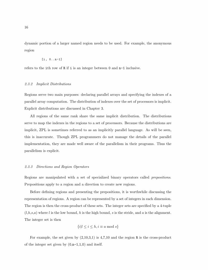
dynamic portion of a larger named region needs to be used. For example, the anonymous

region

[i , 0..n-1]

refers to the ith row of R if i is an integer between 0 and n-1 inclusive.

2.3.2 Implicit Distributions

Regions serve two main purposes: declaring parallel arrays and specifying the indexes of a

parallel array computation. The distribution of indexes over the set of processors is implicit.

Explicit distributions are discussed in Chapter 3.

All regions of the same rank share the same implicit distribution. The distributions

serve to map the indexes in the regions to a set of processors. Because the distributions are

implicit, ZPL is sometimes referred to as an implicitly parallel language. As will be seen,

this is inaccurate. Though ZPL programmers do not manage the details of the parallel

implementation, they are made well aware of the parallelism in their programs. Thus the

parallelism is explicit.

2.3.3 Directions and Region Operators

Regions are manipulated with a set of specialized binary operators called prepositions.

Prepositions apply to a region and a direction to create new regions.

Before defining regions and presenting the prepositions, it is worthwhile discussing the

representation of regions. A region can be represented by a set of integers in each dimension.

The region is then the cross-product of these sets. The integer sets are specified by a 4-tuple

(l,h,s,a) where l is the low bound, h is the high bound, s is the stride, and a is the alignment.

The integer set is then

{i|l ≤ i ≤ h, i ≡ a mod s}

For example, the set given by (2,10,3,1) is 4,7,10 and the region R is the cross-product

of the integer set given by (0,n-1,1,0) and itself.

17

Directions

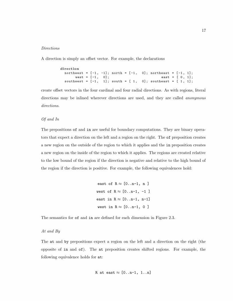
A direction is simply an offset vector. For example, the declarations

direction

northwest = [ -1 , -1]; north = [-1, 0]; northeast = [ -1 , 1];

west = [-1, 0]; east = [ 0 , 1];

southwest = [-1, 1]; south = [ 1 , 0]; southeast = [ 1 , 1];

create offset vectors in the four cardinal and four radial directions. As with regions, literal

directions may be inlined wherever directions are used, and they are called anonymous

directions.

Of and In

The prepositions of and in are useful for boundary computations. They are binary opera-

tors that expect a direction on the left and a region on the right. The of preposition creates

a new region on the outside of the region to which it applies and the in preposition creates

a new region on the inside of the region to which it applies. The regions are created relative

to the low bound of the region if the direction is negative and relative to the high bound of

the region if the direction is positive. For example, the following equivalences hold:

east of R ≈ [0..n-1, n ]

west of R ≈ [0..n-1, -1 ]

east in R ≈ [0..n-1, n-1]

west in R ≈ [0..n-1, 0 ]

The semantics for of and in are defined for each dimension in Figure 2.3.

At and By

The at and by prepositions expect a region on the left and a direction on the right (the

opposite of in and of). The at preposition creates shifted regions. For example, the

following equivalence holds for at:

R at east ≈ [0..n-1, 1..n]

18

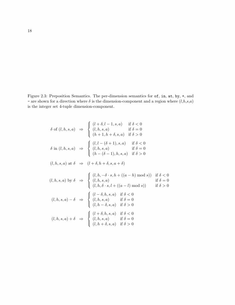
Figure 2.3: Preposition Semantics. The per-dimension semantics for of, in, at, by, +, and- are shown for a direction where δ is the dimension-component and a region where (l,h,s,a)is the integer set 4-tuple dimension-component.

δ of (l, h, s, a) ⇒

(l + δ, l − 1, s, a) if δ < 0(l, h, s, a) if δ = 0(h + 1, h + δ, s, a) if δ > 0

δ in (l, h, s, a) ⇒

(l, l − (δ + 1), s, a) if δ < 0(l, h, s, a) if δ = 0(h − (δ − 1), h, s, a) if δ > 0

(l, h, s, a) at δ ⇒ (l + δ, h + δ, s, a + δ)

(l, h, s, a) by δ ⇒

(l, h,−δ · s, h + ((a − h) mod s)) if δ < 0(l, h, s, a) if δ = 0(l, h, δ · s, l + ((a − l) mod s)) if δ > 0

(l, h, s, a) − δ ⇒

(l − δ, h, s, a) if δ < 0(l, h, s, a) if δ = 0(l, h − δ, s, a) if δ > 0

(l, h, s, a) + δ ⇒

(l + δ, h, s, a) if δ < 0(l, h, s, a) if δ = 0(l, h + δ, s, a) if δ > 0

19

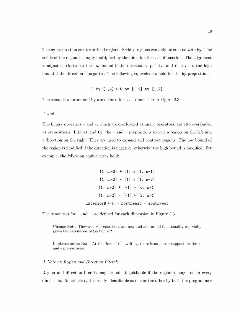
The by preposition creates strided regions. Strided regions can only be created with by. The

stride of the region is simply multiplied by the direction for each dimension. The alignment

is adjusted relative to the low bound if the direction is positive and relative to the high

bound if the direction is negative. The following equivalences hold for the by preposition:

R by [1,4] ≈ R by [1,2] by [1,2]

The semantics for at and by are defined for each dimension in Figure 2.3.

+ and -

The binary operators + and -, which are overloaded as unary operators, are also overloaded

as prepositions. Like at and by, the + and - prepositions expect a region on the left and

a direction on the right. They are used to expand and contract regions. The low bound of

the region is modified if the direction is negative; otherwise the high bound is modified. For

example, the following equivalences hold:

[1..n-2] + [1] ≈ [1..n-1]

[1..n-2] - [1] ≈ [1..n-3]

[1..n-2] + [-1] ≈ [0..n-1]

[1..n-2] - [-1] ≈ [2..n-1]

InteriorR ≈ R - northeast - southwest

The semantics for + and - are defined for each dimension in Figure 2.3.

Change Note. The+ and - prepositions are new and add useful functionality especiallygiven the extensions of Section 4.2.

Implementation Note. At the time of this writing, there is no parser support for the +and - prepositions.

A Note on Region and Direction Literals

Region and direction literals may be indistinguishable if the region is singleton in every

dimension. Nonetheless, it is easily identifiable as one or the other by both the programmer

20

and the compiler based on the context. For example, the following equivalences are easy to

verify:

[1,1] of [2,2] ≈ [3,3]

[2,2] of [1,1] ≈ [2..3,2..3]

2.3.4 Region Types

Regions are first-class in ZPL. They are typed constructs and their rank is part of their type.

As new concepts are introduced, the type of the region will be expanded. For example, in

addition to a region’s rank, the type of each of its dimensions is part of its type. So far, only

one dimension type, range, has been introduced so this is uninteresting. Section 2.8 will

introduce a second dimension type and Chapter 4 will introduce a third and final dimension

type.

The syntax used for declaring regions previously is a useful syntactic sugar for declaring

constant regions. Regions R, InteriorR, TopRow, and Line could also be declared using the

following syntax:

const R : region <.. ,.. > = [0..n -1 , 0..n -1];

InteriorR : region <.. ,.. > = [1..n -2 , 1..n -2];

TopRow : region <.. ,.. > = [0 , 0..n -1];

Line : region <..> = [0..n -1];

The “..” portion of the region type specifies that a region is declared with dimension type

range in the dimension. Two more dimension types will be introduced later in this thesis:

flood dimensions in Section 2.8 and grid dimensions in Chapter 4. Note that for initialized

regions it is legal to declare the type simply as region since the dimension types can be

inferred. For variable regions that are not initialized this type information is necessary.

Change Note. The extensions in this thesis made it necessary to distinguish betweena region’s value and type. Previously, it was unclear whether a region was a type or avalue and regions were never variables or constants.

21

2.3.5 Sparse Regions

Sparse regions allow programmers to specify sparse computations over both sparse and dense

arrays using syntax similar to masks. By separating the sparse index set from the array,

programmers are able to express their sparse computations using a dense array syntax,

making the code easier for programmers to read and compilers to optimize. Sparse regions

are an important concept in ZPL. Their existence has influenced some of the choices made

in this thesis. Nonetheless, they are a complicated subject that is largely orthogonal to the

work in this thesis. The reader interested in learning more about ZPL’s support for sparse

computations is referred to the literature [CLS98, CS01, Cha01].

2.4 Parallel Arrays

As mentioned, regions are used to declare parallel arrays and to specify the indexes of a

parallel array computation. ZPL is first and foremost a parallel array language. The region

is its central abstraction, but regions are useless without parallel arrays. For simplicity, this

thesis will refer to parallel arrays simply as arrays. Where the distinction between parallel

arrays and indexed arrays is unclear, indexed arrays will be called indexed arrays.

2.4.1 Arrays and Regions

Regions have no associated data. Arrays are declared over regions and contain data for each

index in its declaring region. For example, the declarations

var A, B, C : [R] integer ;

L : [ Line ] integer ;

create three arrays, A, B, and C, that contain n2 integers each and one array, L, that contains

n integers. The scalar type component of these arrays, integer, is called the base type. The

type of a parallel array consists of the base type and the type of the declaring region. The

region itself is not part of the type of the array, although it is statically bound to the array.

Parallel arrays are distributed across the processors according to their region distribu-

tion. Thus, if explicit distributions are not used, all parallel arrays of the same rank are

distributed in the same way. This allows all basic array computations to execute in paral-

22

lel without any interprocessor communication. Communication is only induced by ZPL’s

parallel operators (introduced in Section 2.5).

Basic array computations are elementwise and data-parallel. They are written with a

region that specifies the indexes involved in the computation. For example, the statement

[InteriorR ] A := B + C;

assigns the elementwise sums of the interior elements of B and C to the corresponding

elements of A. Note that the computing region can be different from the declaring region.

2.4.2 Arrays and Structured Types

Unlike indexed arrays, parallel arrays may not be nested. However, parallel arrays can be

nested inside indexed arrays and records and these structured types can be the base types

of parallel arrays. For example, the declarations

var AofI : [R] array [0..n -1] of integer ;

IofA : array[0..n -1] of [R] integer ;

create two structures. The parallel array of indexed arrays AofI distributes indexed arrays

across the processors. The indexed array of parallel arrays IofA contains an indexed array

of parallel arrays that distribute the integers. Their storage and parallel implementation is

different, but they are referenced in the same way. For example, the statement

[R] AofI [] := IofA [];

assigns all of the elements of IofA to AofI.

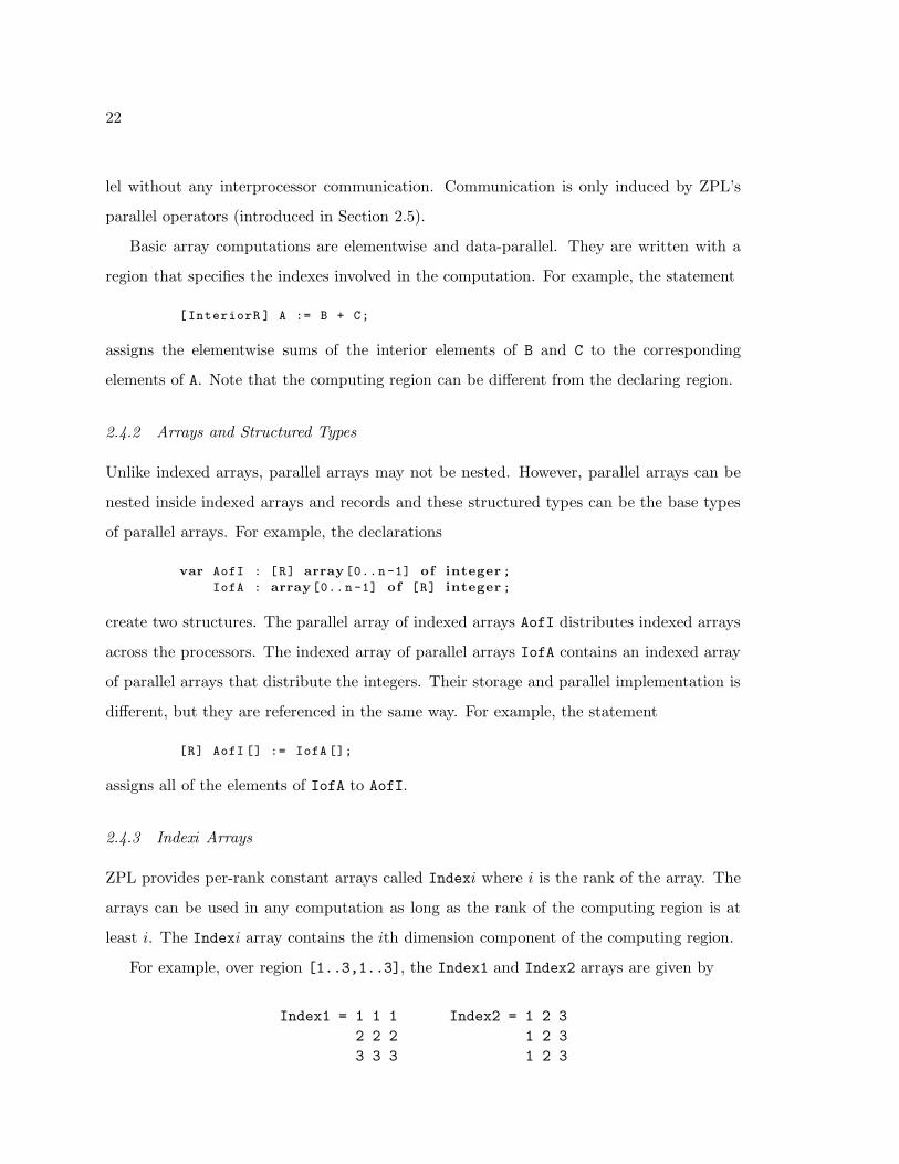
2.4.3 Indexi Arrays

ZPL provides per-rank constant arrays called Indexi where i is the rank of the array. The

arrays can be used in any computation as long as the rank of the computing region is at

least i. The Indexi array contains the ith dimension component of the computing region.

For example, over region [1..3,1..3], the Index1 and Index2 arrays are given by

Index1 = 1 1 1 Index2 = 1 2 3

2 2 2 1 2 3

3 3 3 1 2 3

23

P-Independent Note. In the definition of the language so far, all behavior is p-independent.This follows because the semantics of the language are orthogonal to the processors.

2.5 Parallel Operators

Communication between processors is an expensive part of parallel computing that should

be avoided when possible. For interesting parallel computations, communication can be

minimized, but it is impossible to avoid completely. In ZPL, unlike many other high-level

parallel programming languages, communication is syntactically identifiable. Communica-

tion is induced only by the following operators: @, @^, op<<, op||, >>, #, and ’@. The

advantages of syntactically identifiable communication are great not only for programmers

who can easily evaluate the quality of their code, but also for the compiler which can eas-

ily optimize local portions of the code. These operators are collectively referred to as the

parallel operators.

This section presents the parallel operators and shows examples to acquaint the reader

with their semantics. The most important point about ZPL’s semantics is that it is an

array language and thus the right hand side of an expression can be evaluated before the

left hand side. Temporary variables declared over the computing region can be inserted for

every expression. The one exception to this rule is with statements involving the prime at,

(’@), operator. More exceptions will be discussed in Chapter 4. The semantics introduced

here are a simpler form of the full semantics. They are complete as regarding parallel arrays

with range dimensions and scalars.

2.5.1 The @ and Wrap @ Operators

The @ operator, (@), and the wrap @ operator, (@^), are useful for nearest neighbor and

stencil computations. The @ operator shifts data in an array by a direction similarly to

how the at preposition shifts indexes in a region. The wrap @ operator also shifts data in

an array by a direction and, in addition, applies a toroidal boundary condition to the array.

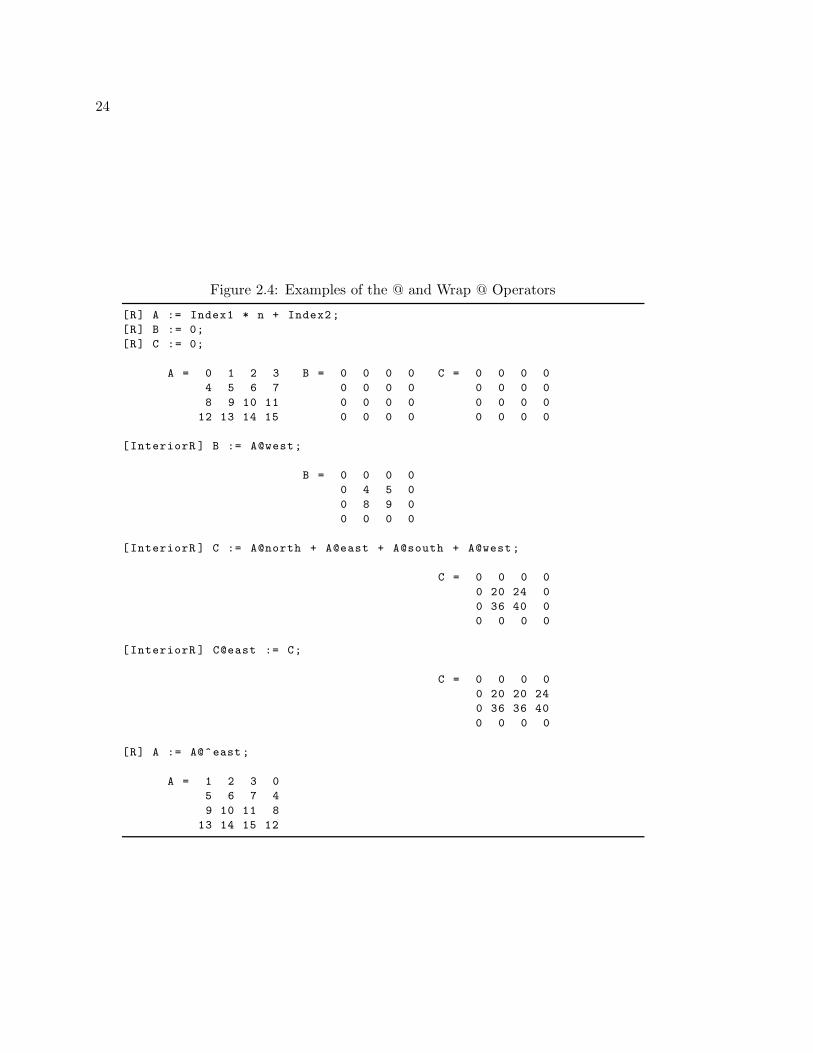
Figure 2.4 shows several examples of applying the @ operator to parallel arrays. The

first segment of code initializes arrays A, B, and C from Section 2.4.1. Array A is initialized

with the Indexi arrays so that each element in A is unique; arrays B and C are zeroed out.

24

Figure 2.4: Examples of the @ and Wrap @ Operators

[R] A := Index1 * n + Index2;

[R] B := 0;

[R] C := 0;

A = 0 1 2 3 B = 0 0 0 0 C = 0 0 0 0

4 5 6 7 0 0 0 0 0 0 0 0

8 9 10 11 0 0 0 0 0 0 0 0

12 13 14 15 0 0 0 0 0 0 0 0

[InteriorR ] B := A@west;

B = 0 0 0 0

0 4 5 0

0 8 9 0

0 0 0 0

[InteriorR ] C := A@north + A@east + A@south + A@west;

C = 0 0 0 0

0 20 24 0

0 36 40 0

0 0 0 0

[InteriorR ] C@east := C;

C = 0 0 0 0

0 20 20 24

0 36 36 40

0 0 0 0

[R] A := A@^east ;

A = 1 2 3 0

5 6 7 4

9 10 11 8

13 14 15 12

25

The next line shows a simple assignment statement from A to B where the @ operator

has been applied to A and the direction west. Note that the assignment takes place over

region InteriorR. Thus only the interior elements of B are assigned values. They are the

values in the region InteriorR at west.

The third line shows a more interesting computation. Here the interior elements of C

are assigned the sum of the four neighbors to the corresponding interior elements of A.

The fourth line shows how the @ operator can be applied to the left-hand side of a

statement. The @ operator, wrap @ operator, ’@ operator, and remap operator may all be

used on the left-hand side. The other parallel operators can only be used on the right-hand

side. In this example, the data in the interior of C is shifted to the right.

The last line shows a use of the wrap @ operator. In this line, the values of A are cyclically

shifted to the left. As mentioned previously, because ZPL is an array programming language,

the right hand side of a statement is evaluated before the left hand side.

2.5.2 The Reduce Operator

The reduce operator is used to compute reductions. It supports two types of reductions

called full reductions and partial reductions. In full reductions, the elements of a parallel

array read over some region are combined to form a single scalar value. In partial reductions,

the elements of a parallel array read over some region are reduced in one or more dimensions

to the same or another parallel array.

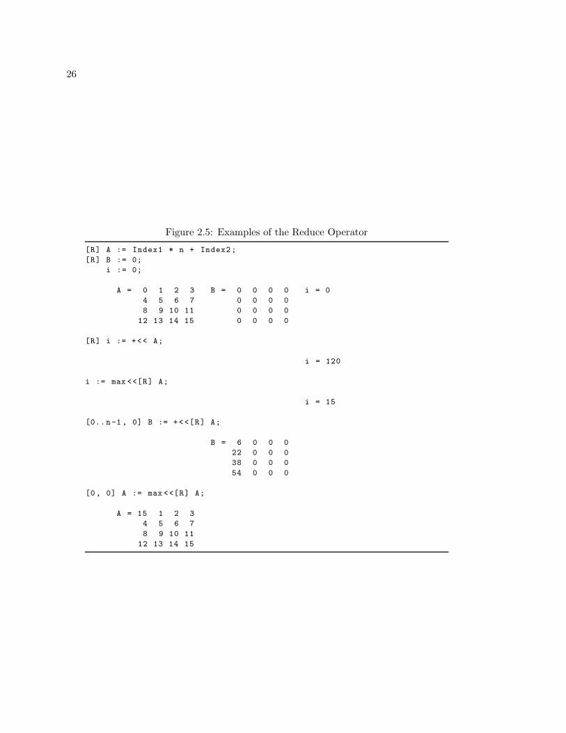
Figure 2.5 shows several examples of applying the reduce operator to parallel arrays.

The first example of the reduce operator shows a full reduction of A. Since R specifies all

the elements in A, the first example stores into i the sum of all of the elements in A. The

second example shows a full reduction using the max operator instead of the + operator and

using an alternative syntax. The result is the same; the scalar i is assigned the maximum

element in A.

Change Note. This new syntax for full reductions is new to ZPL. It makes for a moresymmetric language definition.

Implementation Note. At the time of this writing, this alternative syntax is not sup-

26

Figure 2.5: Examples of the Reduce Operator

[R] A := Index1 * n + Index2;

[R] B := 0;

i := 0;

A = 0 1 2 3 B = 0 0 0 0 i = 0

4 5 6 7 0 0 0 0

8 9 10 11 0 0 0 0

12 13 14 15 0 0 0 0

[R] i := +<< A;

i = 120

i := max <<[R] A;

i = 15

[0..n-1 , 0] B := +<<[R] A;

B = 6 0 0 0

22 0 0 0

38 0 0 0

54 0 0 0

[0 , 0] A := max <<[R] A;

A = 15 1 2 3

4 5 6 7

8 9 10 11

12 13 14 15

27

ported.

The third and fourth examples show partial reductions. In the third example, the second

dimension of array A is reduced. The first column of B is assigned the sum of the rows of

array A. In the fourth example, the element at position (0,0) in array A is assigned the

maximum element in A.

The semantics of the reduce operator are simple. Full reductions are always assigned to

scalar variables; they are always applied to parallel arrays. Partial reductions are always

assigned to and from parallel arrays. For partial reductions, there are two regions, a source

region and a destination region. The source region applies to the array or array expression

being reduced. The destination region applies to the result. A dimension is reduced if

the source region is a range in that dimension and the destination region is a singleton in

that dimension. If the destination dimension is a range, the source dimension must be the

identical range. If the source dimension is a singleton, the destination dimension must be

another, not necessarily identical, singleton.

The semantics do not require the source to be a range and the destination to be a

singleton so as to allow for partial multi-dimensional reductions (such as the third reduction

in Figure 2.5. Note that one can use the reduction operator to write a simple assignment

between two arrays as in

[R] A := +<<[R] A;

In this case, since no dimensions are reduced, nothing is done.

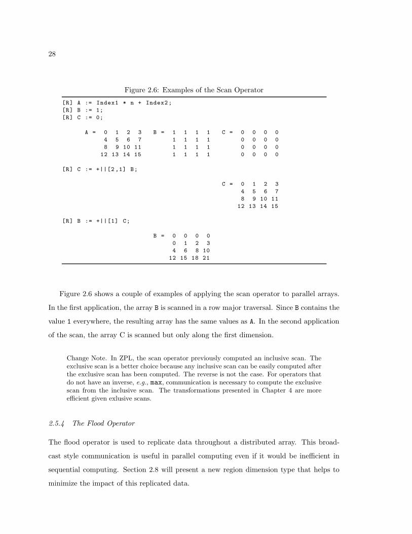
2.5.3 The Scan Operator

The scan operator computes parallel prefix computations. The programmer specifies a

dimension list that looks like a direction or region of singleton dimensions where every

dimension has a unique integer from one to the rank. The length of the dimension list

can be no longer than the rank of the computing region. The dimension list orders the

scan over the dimensions. The scan operator then uses the operator to compute exclusive

prefix reductions throughout the computing region. In the exclusive scan, as opposed to an

inclusive scan, the last element is not included in the prefix reduction.

28

Figure 2.6: Examples of the Scan Operator

[R] A := Index1 * n + Index2;

[R] B := 1;

[R] C := 0;

A = 0 1 2 3 B = 1 1 1 1 C = 0 0 0 0

4 5 6 7 1 1 1 1 0 0 0 0

8 9 10 11 1 1 1 1 0 0 0 0

12 13 14 15 1 1 1 1 0 0 0 0

[R] C := +||[2 ,1] B;

C = 0 1 2 3

4 5 6 7

8 9 10 11

12 13 14 15

[R] B := +||[1] C;

B = 0 0 0 0

0 1 2 3

4 6 8 10

12 15 18 21

Figure 2.6 shows a couple of examples of applying the scan operator to parallel arrays.

In the first application, the array B is scanned in a row major traversal. Since B contains the

value 1 everywhere, the resulting array has the same values as A. In the second application

of the scan, the array C is scanned but only along the first dimension.

Change Note. In ZPL, the scan operator previously computed an inclusive scan. Theexclusive scan is a better choice because any inclusive scan can be easily computed afterthe exclusive scan has been computed. The reverse is not the case. For operators thatdo not have an inverse, e.g., max, communication is necessary to compute the exclusivescan from the inclusive scan. The transformations presented in Chapter 4 are moreefficient given exlusive scans.

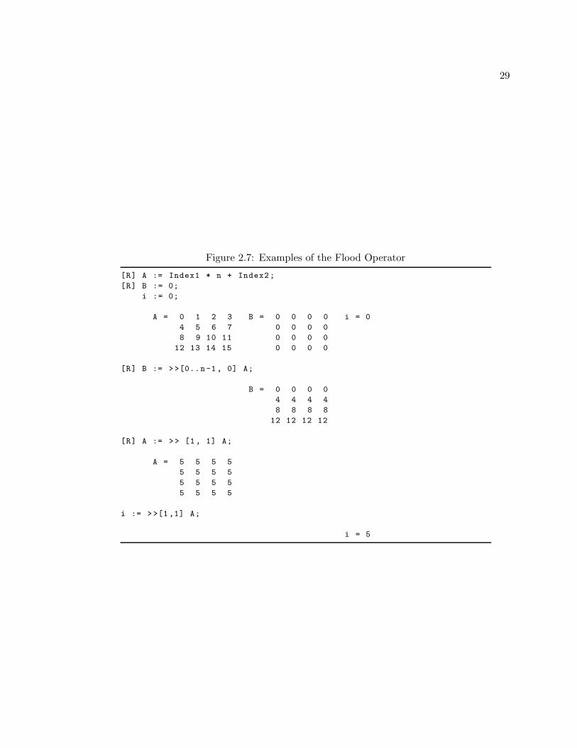
2.5.4 The Flood Operator

The flood operator is used to replicate data throughout a distributed array. This broad-

cast style communication is useful in parallel computing even if it would be inefficient in

sequential computing. Section 2.8 will present a new region dimension type that helps to

minimize the impact of this replicated data.

29

Figure 2.7: Examples of the Flood Operator

[R] A := Index1 * n + Index2;

[R] B := 0;

i := 0;

A = 0 1 2 3 B = 0 0 0 0 i = 0

4 5 6 7 0 0 0 0

8 9 10 11 0 0 0 0

12 13 14 15 0 0 0 0

[R] B := > >[0..n -1 , 0] A;

B = 0 0 0 0

4 4 4 4

8 8 8 8

12 12 12 12

[R] A := > > [1 , 1] A;

A = 5 5 5 5

5 5 5 5

5 5 5 5

5 5 5 5

i := > >[1 ,1] A;

i = 5

30

Figure 2.7 shows several examples of applying the flood operator to parallel arrays. In

the first application of the flood operator, the first column of A is replicated throughout the

columns of B. Notice that with the flood operator, like with the reduce operator, there are

two regions, a source region and a destination region. In the case of the flood, a dimension

is replicated if the source dimension is a singleton and the destination dimension is a range.

This is the opposite of reduce. In the case of flood, if the source dimension is a range

and the destination dimension is a range, they must be identical ranges. If the destination

dimension is a singleton, the source dimension must be another, not necessarily identical,

singleton.

In the second application of the flood operator, the element at position (1,1) in array A

is replicated throughout the whole of A. The third application of the flood operator shows

a full flood. This is the logical counterpart to the full reduce. In the full flood, a single

element in a parallel array is moved into a scalar variable. Note that in this case, A has the

same value everywhere so the specified position does not matter. Nonetheless, even in the

presence of a high-quality optimizing compiler, the flood operator could still need to induce

communication here if, for example, there are processors that do not own any of A.

Change Note. Previously there was no counterpart to the full reduction; the full flooddid not exist. Rather, the full reduction operator was used in this case and the operatorwas ignored.

Implementation Note. At the time of this writing, full floods are not supported.

In the definition of the language so far, there are no p-dependent abstractions. Thisfollows because the semantics are independent of the processors. Moreover, where com-munication does exist, there is no possibility that the logical values will change depend-ing on the processors. Round-off error in reductions and scans is ignored as mentionedin the introduction. The next operator is different because of a many-to-one mappingwhich may change depending on the processors.

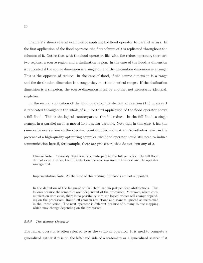
2.5.5 The Remap Operator

The remap operator is often referred to as the catch-all operator. It is used to compute a

generalized gather if it is on the left-hand side of a statement or a generalized scatter if it

31

Figure 2.8: Examples of the Remap Operators

[R] A := Index1 * n + Index2;

[R] B := n - 1 - Index1;

[Line ] L := Index1 * n;

A = 0 1 2 3 B = 3 3 3 3 L = 0 4 8 12

4 5 6 7 2 2 2 2

8 9 10 11 1 1 1 1

12 13 14 15 0 0 0 0

[R] A := A#[Index2 , Index1 ];

A = 0 4 8 12

1 5 9 13

2 6 10 14

3 7 11 15

[R] B := A#[B , ];

B = 3 7 11 15

2 6 10 14

1 5 9 13

0 4 8 12

[R] A := L#[ Index2 ];

A = 0 4 8 12

0 4 8 12

0 4 8 12

0 4 8 12

[Line ] L := B#[ Index1 ,Index1 ];

L = 3 6 9 12

32

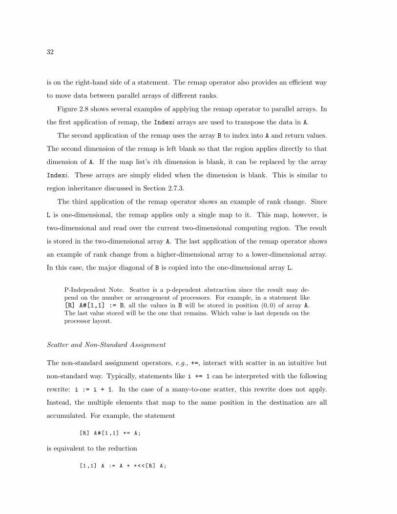
is on the right-hand side of a statement. The remap operator also provides an efficient way

to move data between parallel arrays of different ranks.

Figure 2.8 shows several examples of applying the remap operator to parallel arrays. In

the first application of remap, the Indexi arrays are used to transpose the data in A.

The second application of the remap uses the array B to index into A and return values.

The second dimension of the remap is left blank so that the region applies directly to that

dimension of A. If the map list’s ith dimension is blank, it can be replaced by the array

Indexi. These arrays are simply elided when the dimension is blank. This is similar to

region inheritance discussed in Section 2.7.3.

The third application of the remap operator shows an example of rank change. Since

L is one-dimensional, the remap applies only a single map to it. This map, however, is

two-dimensional and read over the current two-dimensional computing region. The result

is stored in the two-dimensional array A. The last application of the remap operator shows

an example of rank change from a higher-dimensional array to a lower-dimensional array.

In this case, the major diagonal of B is copied into the one-dimensional array L.

P-Independent Note. Scatter is a p-dependent abstraction since the result may de-pend on the number or arrangement of processors. For example, in a statement like[R] A#[1,1] := B, all the values in B will be stored in position (0, 0) of array A.The last value stored will be the one that remains. Which value is last depends on theprocessor layout.

Scatter and Non-Standard Assignment

The non-standard assignment operators, e.g., +=, interact with scatter in an intuitive but

non-standard way. Typically, statements like i += 1 can be interpreted with the following

rewrite: i := i + 1. In the case of a many-to-one scatter, this rewrite does not apply.

Instead, the multiple elements that map to the same position in the destination are all

accumulated. For example, the statement

[R] A#[1 ,1] += A;

is equivalent to the reduction

[1 ,1] A := A + +<<[R] A;

33

Figure 2.9: Examples of the Prime @ Operator

[R] A := Index1 * n + Index2;

[R] B := 1;

A = 0 1 2 3 B = 1 1 1 1

4 5 6 7 1 1 1 1

8 9 10 11 1 1 1 1

12 13 14 15 1 1 1 1

[InteriorR ] A := A’@west;

A = 0 1 2 3

4 4 4 7

8 8 8 11

12 13 14 15

[1..n-1 , 1..n -1] B := B’@north + B’@west;

B = 1 1 1 1

1 2 3 4

1 3 6 10

1 4 10 20

[0..n-2 , 0..n -2] interleave

A := B’@[1 ,1];

B := A + A’@east;

end;

A = 41 17 4 3 B = 58 21 7 1

30 31 10 7 61 41 17 4

4 10 20 11 14 30 31 10

12 13 14 15 1 4 10 20

It is not equivalent to the statement

[R] A#[1 ,1] := A#[1 ,1] + A;

2.5.6 The Prime @ Operator and Interleave

The prime @ operator, ’@, provides language-level support for representing wavefront

computations. This operator is briefly noted here. For a more thorough discussion of

ZPL’s support for pipelining wavefront computations, the reader is referred to the litera-

ture [CLS99a, LS00, Lew01].

The prime @ operator breaks the array language semantics of evaluating the right-hand

34

side before evaluating the left-hand side. For statements involving the prime @ operator, the

statement cannot be rewritten with temporary arrays declared over the computing region

used to store temporary expressions. For this reason, the prime @ operator is restricted to

statements that contain only @, wrap @, and other prime @ operators. In addition, when

multiple directions are used in these statements, there are restrictions on the values of these

directions that make sense.

The prime @ operator denotes an array whose values should be reused in the computation

after they are created. The directions thus induce an order on the computation called a

wavefront. Multiple statements can be involved in these wavefronts using interleaved blocks.

The interleave keyword requires multiple statements to be executed together.

In addition to being useful for wavefront computations, interleaving statements lets the

programmer manually implement the scalarizing compiler optimization of loop fusion. In-

terleaving statements can be interpreted as executing the block of statements for each index

separately. ZPL’s sequential flow of parallel statements is violated in interleaved statement

blocks. For this reason, communication is limited in interleave blocks to avoid the issues

plaguing languages involving a parallel execution of communicating sequential processes.

Such CSP style languages imply the possibility of deadlocks and race conditions which are

impossible in ZPL. Interleaved statement blocks are subject to the same restrictions as sin-

gle statements involving a prime @ operator. Other than the @, wrap @, and prime @

operators, no other parallel operators may be used in interleaved statements. In addition,

scalars may not be assigned values in interleaved statement blocks.

Change Note. Previously, multiple statements could be executed in a single wavefrontusing a scan block rather than an interleave block. The semantics were identical,but the keyword was different. By changing the keyword to interleave and giving ita more general meaning, the single concept can be reused. The interleave keywordis especially useful when combined with the extensions of Chapter 4.

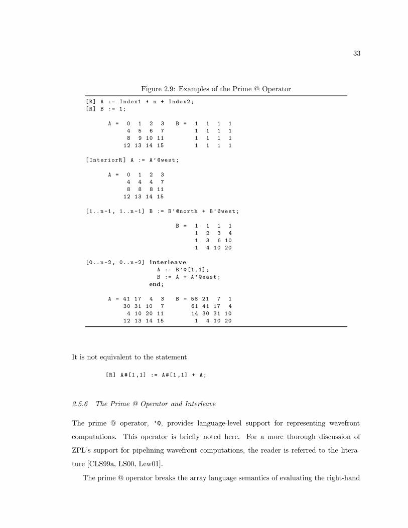
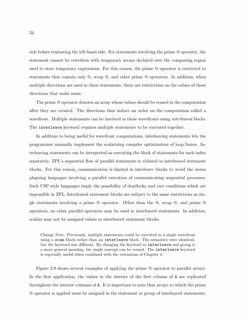
Figure 2.9 shows several examples of applying the prime @ operator to parallel arrays.

In the first application, the values in the interior of the first column of A are replicated

throughout the interior columns of A. It is important to note that arrays to which the prime

@ operator is applied must be assigned in the statement or group of interleaved statements.

35

Otherwise, there would be no newly created values to read.

In the second application of the prime @ operator, a wavefront computation is induced

from the upper-left corner of B. Each element not in the first row or column of B is assigned

the sum of its neighbor to the north and west as the wavefront passes by.

The last application of the prime @ operator shows a more complicated set of interacting

wavefronts using two interleaved statements. A pipelined implementation of this code is very

difficult to write in a lower-level language like Fortran+MPI. It is also very important to

pipeline such wavefronts because they are important in many applications. The prime @

operator makes the code easy to write and guarantees a parallel implementation.

P-Independent Note. The Prime @ operator is p-independent.

2.5.7 ZPL’s Parallel Performance Model

Knowing that the parallel operators induce communication lets programmers optimize their

programs or choose between alternative algorithms if it can be determined that one program

induces significantly more communication than the other. In addition to this knowledge,

the programmer knows that some parallel operators are more expensive than others. The

@ operator’s nearest neighbor communication is significantly cheaper than the remap op-

erator’s remap communication in the worst case. The other operators lie between these

two extremes. For a more detailed discussion of this important ZPL property, the reader is

referred to the literature [CCL+98b].

2.5.8 A Note on Structured Parallel Arrays

The @, wrap @, prime @, and remap operators apply to parallel arrays and result in variables

that can be assigned much like indexing into indexed arrays and selecting fields of records.

However, unlike array indexing and field selection, these operators do not apply to the point

in the type where the region is used to declare a parallel array. They always apply to the

outside. For example, when the @ operator is applied to AofI and IofA from Section 2.4.2,

the expressions are as follows:

[R] ... AofI [i]@east ... IofA [i]@east ...

36

This is particularly important for cases where the indexing is done by a parallel array. For

example, if i is replaced by A, the @ operator applies to both AofI, IofA, and A. This allows

us to maintain the performance model. If the @ operator did not apply to the A in either

case, extra communication would be necessary to pass the values of A onto the processor

that is reading or writing AofI and IofA. The excess communication is even worse in the

case of the remap operator.

Change Note. Previously, the @ and remap operators did not apply to the outside ofthe expression, but rather to the point where the region was used in the declaration.This was an oversight. It is not too difficult to derive an example that would violatethe performance model if the operator did not apply to everything to its left. Thoughrare, examples of a similar nature are common with the extensions of Chapter 4.

2.6 Promotion

Promotion is a natural concept in ZPL in which scalar operators, values, procedures, and

control structures seamlessly interact with parallel arrays. Virtually transparent, promotion

has already been introduced. For example, in the simple statement

[R] C := A + B;

the scalar operators := and + were promoted to operate element-wise on the parallel arrays.

2.6.1 Scalar Value Promotion

Promotion of scalar values has also been seen before. If a parallel array activates a statement,

all scalar variables and values in that statement are transparently promoted. For example,

in the statement

[R] C := C + 1;

the value 1 becomes a parallel array of 1s. Similarly, a scalar variable would become a

parallel array of the same base type with its value replicated.

Values can only be promoted for reading, not writing. Thus a parallel array cannot be

assigned to a scalar. This error is caught by the type checker, ensuring that scalars are kept

consistent across the processors. For example, the following line of code does not compute

37

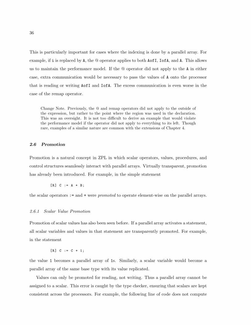
Listing 2.4: An Example of Scalar Procedure Promotion

1 procedure add(a, b : integer ; out c : integer );

2 begin

3 c := a + b;

4 end;

6 [InteriorR ] add(A, B, C);

a reduction over parallel array A:

[R] i += A;

Instead it results in a type-checking error.

2.6.2 Scalar Procedure Promotion

Scalar procedures are procedures that do not involve parallel arrays and call only other

scalar procedures. Scalar procedures can be promoted in a similar way to scalar operators if

and only if they have no side effects. For example, Listing 2.4 shows an example in which a

scalar add procedure that takes two integers and stores their sum in a third can be promoted

to work on three parallel arrays.

A scalar procedure is promoted if it is called from a statement to which a region applies,

i.e., there are parallel arrays in that statement even if not in the arguments to the function.

Change Note. A scalar procedure only used to be promoted if one or more of itsarguments were parallel arrays. Thus if it was assigned to a parallel array, its resultwould be promoted but the procedure would not be. These old semantics do not meshwell with the extension of Chapter 4 or shattered control flow (introduced shortly).

When a scalar procedure is promoted, all its arguments are promoted. A scalar argument

can thus not be passed to any of the promoted procedure’s out and inout parameters. In

addition, the procedure’s return value is promoted and cannot be assigned to a scalar.

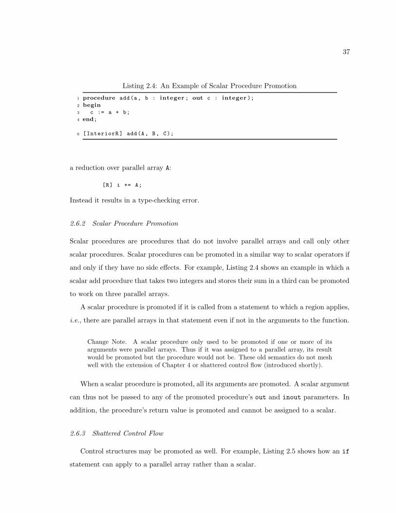
2.6.3 Shattered Control Flow

Control structures may be promoted as well. For example, Listing 2.5 shows how an if

statement can apply to a parallel array rather than a scalar.

38

Listing 2.5: An Example of Scalar Procedure Promotion

1 [R] i f A < 0 then

2 B := -A;

3 e lse

4 B := A;

5 end;

Shattered control flow results in code similar to interleave statements, discussed in Sec-

tion 2.5.6. The statements in the control flow block are executed for each index. The parallel

operators may not be used in shattered control flow and scalars may not be assigned within

shattered control flow.

Note that shattered control flow, interleaved statement blocks, and promoted scalar pro-

cedures are all similar. They all replace ZPL’s sequential composition of parallel statements

with a parallel execution of statements for each index. The restrictions associated with

each of these concepts eliminates the possibility of a parallel composition of communicating

sequential processes.

P-Independent Note. Promotion and shattered control flow are p-independent becausethe semantics are orthogonal to the processors.

2.7 Region Scopes

Region scopes can be opened over single statements, compound statements, or control flow

statements, but a region only actively applies to statements that contain parallel arrays. If

a statement contains no parallel arrays, the region is ignored. Thus regions are said to be

passive. For example, region R serves no purpose in the following line of code (assuming i

is a scalar integer):

[R] i := i + 1;

It is good ZPL style to capitalize parallel arrays and regions while leaving non-parallel

variables, e.g., scalars and indexed arrays, lowercase. This serves as a visual clue to whether

a region is active or passive for any given statement.

39

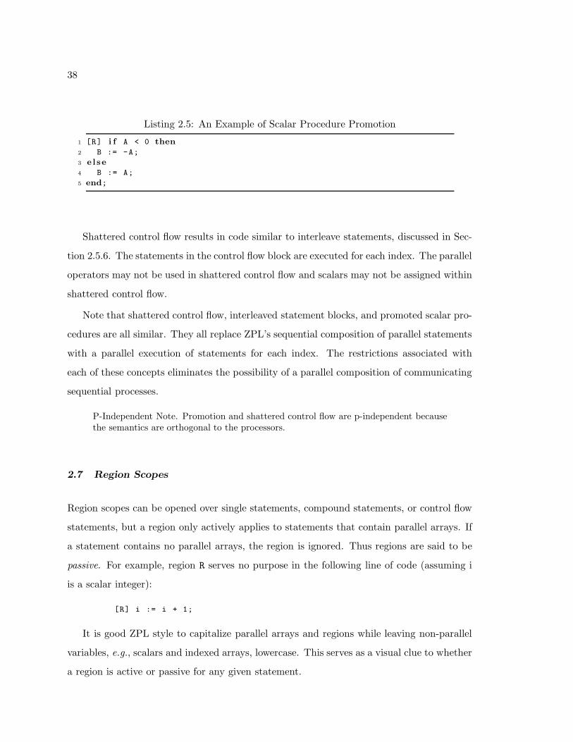
Listing 2.6: An Example of a Dynamic Region Scope

1 procedure Add(A, B : [R] integer ; inout C : [R] integer );

2 begin

3 C := A + B;

4 end;

6 [InteriorR ] Add(A, B, C);

Region scopes may be nested. In these cases, only the innermost region applies to

statements involving parallel arrays. The outer regions are eclipsed.

2.7.1 Dynamic Region Scopes

A region scope may also span procedures. That is, regions are dynamically, not lexically,

scoped. Listing 2.6 shows an example of a dynamically scoped region. In this example,

region InteriorR applies to the parallel procedure call Add. Because it is not eclipsed in

the procedure body, it is used to implement the array statement C := A + B.

2.7.2 Masked Region Scopes

Masks are parallel arrays of Boolean base type. They can be attached to computing regions

using either the keyword with or without. They specify whether indexes are involved in

the computation (with) or not (without). For example, given a Boolean parallel array M

declared over R, the statement

[R with M] A := B + C;

computes the elementwise sum of B and C and stores the result in A wherever M is true. The

mask must be readable over the region to which it applies but does not need to be declared

over that region.

2.7.3 Region Inheritance

When region scopes are opened, they may inherit one or more dimensions from the eclipsed

region. This is legal in the case where the eclipsed region is dynamically scoped. In this

case, the procedure may have to be cloned depending on the types of the regions. There

40

are two forms of region inheritance: blank dimensions and ditto regions.

Blank Dimensions

Blank dimensions allow the programmer to open a new region scope based on the current

region scope. For example, in the code

[R] begin

A := B;

[i, ] B := C;

end;

the values in B are assigned to A and then the values in the ith row of C are assigned to the

ith row of B.

Blank dimensions are especially useful for writing reductions and floods since the reduce

and flood operators require that non-singleton dimensions are identical, inheritance can save

some redundant specifications. For example, writing

[R] A := > >[1 , 0..n -1] A;

is equivalent to writing

[R] A := > >[1 , ] A;

Ditto Scopes

The ditto region, ["], refers to the region scope. It is useful for creating new regions

using prepositions based on the current region, e.g., [east of "]. Because preprocessors

sometimes complain about non-terminating strings, the ditto region may also be written

with two apostrophes as in [’’].

The ditto specifier may also be used to inherit masks from the current region scope. In

this case, the ditto is used after the keyword with or without.

2.8 Flood Dimensions

Flood dimensions, *, are special dimensions of regions that specify a single value and conform

to any index. They are used to hold data that is logically replicated across dimensions of

41

an array. For example, the declarations

region Row = [* , 0..n -1];

Column = [0..n-1 , * ];

create two regions with one flood dimension and one range dimension. Region Row’s first

dimension is a flood dimension; region Column’s second dimension is a flood dimension.

2.8.1 Flood Arrays

Flood arrays are arrays that are declared over flood regions. They have logically a single

element in their flood dimension that can be read over any index. In the implementation,

the single values are replicated over the flood dimensions and each processor contains a copy.

These copies are kept consistent across the processors in the same way that scalars are kept

consistent across the processors. Flood arrays are declared similarly to regular arrays. For

example, the declarations

var FR : [ Row ] integer ;

FC : [ Column ] integer ;

create flood arrays over Row and Column.

Since flood dimensions conform to any range dimension, flood arrays can be read over

any region. The statement

[R] A := FR * FC;

computes the cross-product of the two replicated vectors FR and FC. Arrays with a flood

dimension that are read over a region not flooded in that dimension are said to be promoted,

in much the same way that scalars are promoted. Promotion of flood arrays is discussed in

more detail in Section 2.8.5.

The inverse of this promotion is not allowed. Arrays not flooded in a dimension cannot be

read or written over a region flooded in that dimension because only one value is associated

with a flood dimension and there are multiple values in non-flooded dimensions. In addition,

arrays not flooded in a dimension cannot be written over regions flooded in that dimension.

This enforces their consistency. Like the consistency of scalars, the consistency of flood

arrays is maintained not by extra communication but rather by a restricted use enforced by

42

type-checking.

2.8.2 Indexi Arrays and Flood Dimensions

The Indexi arrays are closely related to flood arrays. For example, in a two-dimensional

region, Index1 has a single value that is replicated across the second dimension. The second

dimension of Index1 is a flood dimension. Similarly, the first dimension of Index2 is a flood

dimension. In general, every dimension other than the ith dimension of Indexi is a flood

dimension. Thus Indexi is readable over any region as long as the ith region is not a flood

dimension.

2.8.3 Parallel Operators and Flood Dimensions

When parallel operators are used on flood arrays, the same semantics as before apply if the

regions do not have flood dimensions. The flood arrays are simply promoted. (The remap

operator is an exception and this will be discussed shortly.) If the regions involved do have

flood dimensions, the semantics are natural and are explained here.

The @, Wrap @, and Prime @ Operators

The @, wrap @, and prime @ operators are ignored over flood dimensions. Since flood arrays

have infinitely replicated data over the flood dimension, accessing neighboring elements are

naturally the same. For example, the statements

[Row] FR := FR@east + 1;

[Row] FR := FR + 1;

are identical for the same reason that

[R] A := FR@east + 1;

[R] A := FR + 1;

are identical. In the latter statements, FR is promoted and the elements in the rows are

identical. In the former statements, FR is not promoted, but the single data value conforms

across the arrays. Note that in the latter statement, FR@east does not result in an out-of-

bounds error since the flood dimensions can be read over any index in that dimension.

43

The Reduce Operator

There are two cases to consider with the reduce operator: whether the destination region

is flooded or whether the source region is flooded. Since flood dimensions have a logically

singular value, they are similar to singleton dimensions. Values in an array can thus be

reduced into flood dimensions. That is, a dimension is reduced if the destination region is

flooded in that dimension and the source region is a range or a singleton in that dimension.

Note that if the source region is singleton in that dimension, the reduction is over the one

value.

In the other case, when the source region is flooded in a dimension, the reduction is

legal, but it has no effect. The result of the reduction is an array that is flooded in the same

dimension. This array can be read, by promotion, over a range or singleton dimension.

The Scan Operator

Like the @ operator, the scan operator has no effect over flooded dimensions. It is treated

the same way it is treated over singleton dimensions. Since there is only one logical value

in that dimension, there is nothing to scan.

The Flood Operator

The flood operator, as its name suggests, is intimately related to the flood dimension.

Although the reduce operator can be used to move data in a regular array into a flood

array, this is a degenerate case. It is much like a full reduction over a singleton region. The

flood operator does a better job of this because there is no operator to ignore.

In a flood dimension, there are two cases to consider. If the destination region is flooded

in a dimension, then the source region must either be a singleton in that dimension or flooded

in that dimension. If it is a singleton, the value is replicated into the flood dimension. This

is the common usage. If it is flooded as well, there is no effect. In the second case, if the

source region is flooded in a dimension, the source expression, which must be readable over

the flood dimension, is unchanged. It can then be promoted to either a singleton or range

dimension of the destination region.

44

The Remap Operator

The remap operator is more complicated than the other operators. Even if the region is

not flooded in any dimension, the semantics may be impacted if the array being remapped

is flooded. This is different than the other operators in which the array could just be

promoted.

If the region is flooded in some dimension, the effect on the remap operator is minor.

The remapped array or expression does not need to be flooded in that dimension. It is

read with the indexes generated by the maps. All other expressions and arrays, as well as

the map expressions, do need to be flooded in that dimension (or they can be promoted

scalars).

The interesting changes show up when the remapped array is flooded in some dimension.

(Note that if the remapped array is flooded in all of its dimensions, the remap operator has

no effect whatsoever and is trivially uninteresting. The interesting case is when the array

is flooded in some dimensions, but not others.)

In the case of the gather, the map array that applies to a dimension in which the

remapped array is flooded is, in a sense, unnecessary. No matter what values that map

array contains, the result will be the same. The map array, however, can be useful in

specifying an optimized parallel implementation. Since the indexes are distributed over the

processors, different values in the map array could cause different processors to send the

same value to other processors. In the case of the scatter, if the destination array is flooded

in some dimension, there is a difficulty. This is because the maps will generate indexes to

write the destination array and this would break the consistency of flood dimensions. For

this reason, a special flood map is provided to read or write flood arrays.

For example, in the gather

[Column ] FC := FR#[ Index2 ,Index2];

the replicated row array is moved into a replicated column array. The second map array

is unnecessary in the sense that it has no effect on the computation. Since FR is flooded

in the second dimension, no matter what the values fed by the second map, the remapped

values would be the same. The flood map allows the programmer to make this explicit. For

45

example, the gather above and the three gathers below are all equivalent:

[Column] FC := FR#[ Index2 ,1];

[Column] FC := FR#[ Index2 ,*];

[Column] FC := FR#[ Index2 , ];

The scalar map array 1 reads from the first position in the second dimension of FR. This

is the same as all the positions. The flood map * reads from FR as if the region FR is read

over is flooded in the second dimension. In the final gather, the map array is elided and the

result is similar to using Index2.

A scatter can be used for the same computation but, in this case, the only legal imple-

mentation is to use a flood map:

[Row] FC #[*, Index1 ] := FR;

Since FC can only be written over a region flooded in the first dimension, the flood map is

necessary. Gather is only different because the array is being read, not written.

Change Note. The flood map is new and has not appeared in previous literature. Usefulon its own, it is symmetric to an extension of Chapter 4.

Implementation Note. At the time of this writing, the flood map is not implemented.

2.8.4 Region Operators and Flood Dimensions

The region operators of, in, at, by, +, and - can be applied to regions with flood dimensions.

The flood dimensions of the region are unchanged; the range dimensions are changed as

always.

2.8.5 Beyond Promotion: Basic Parallel Type Coercion

Promotion, discussed in Section 2.6, is more formally parallel type coercion. In promotion,

scalars are changed into parallel arrays just as integers are changed into doubles in scalar

type coercion (See Section 2.2.2).

Both scalars and flood arrays can be promoted and read over regions with range dimen-

sions. For example, the statement

46

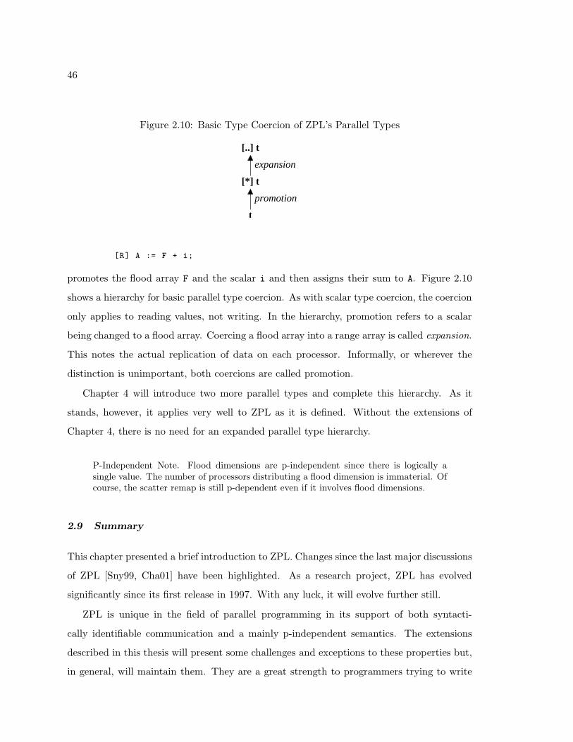
Figure 2.10: Basic Type Coercion of ZPL’s Parallel Types

[*] t

[..] t

t

promotion

expansion

[R] A := F + i;

promotes the flood array F and the scalar i and then assigns their sum to A. Figure 2.10

shows a hierarchy for basic parallel type coercion. As with scalar type coercion, the coercion

only applies to reading values, not writing. In the hierarchy, promotion refers to a scalar

being changed to a flood array. Coercing a flood array into a range array is called expansion.

This notes the actual replication of data on each processor. Informally, or wherever the

distinction is unimportant, both coercions are called promotion.

Chapter 4 will introduce two more parallel types and complete this hierarchy. As it

stands, however, it applies very well to ZPL as it is defined. Without the extensions of

Chapter 4, there is no need for an expanded parallel type hierarchy.

P-Independent Note. Flood dimensions are p-independent since there is logically asingle value. The number of processors distributing a flood dimension is immaterial. Ofcourse, the scatter remap is still p-dependent even if it involves flood dimensions.

2.9 Summary

This chapter presented a brief introduction to ZPL. Changes since the last major discussions

of ZPL [Sny99, Cha01] have been highlighted. As a research project, ZPL has evolved

significantly since its first release in 1997. With any luck, it will evolve further still.

ZPL is unique in the field of parallel programming in its support of both syntacti-

cally identifiable communication and a mainly p-independent semantics. The extensions

described in this thesis will present some challenges and exceptions to these properties but,

in general, will maintain them. They are a great strength to programmers trying to write

47

high-performance parallel programs in a reasonable amount of time.