chapter 3 - mohan munasinghe

3. Economics of the Environment∗ Overview This chapter explores how economics relates to environmental (and related social) concerns. Section 3.1 outlines how environmental degradation is impeding economic development, while human activity is harming the environment. Sections 3.2 and 3.3 expand on economic cost-benefit analysis – a key element of SDA and the project cycle. Important details are explained, including economic decision criteria, efficiency and social shadow pricing, economic imperfections (market failures, policy distortions, and institutional constraints), methods of measuring costs and benefits, and qualitative considerations. Types of environmental assets and services, and practical techniques of valuing them are described in Section 3.4. Next, Section 3.5 outlines multi-criteria analysis, which is useful for decision making, when economic valuation is difficult. Key issues relating to discounting, risk and uncertainty are set out in Section 3.6. Finally, Section 3.7 explains links between economywide policies and environmental (and social) issues, as well as environmentally adjusted national accounts. 3.1 HUMAN ACTIVITIES AND THE ENVIRONMENT Mankind's relationship with the environment has gone through several stages, starting with primitive times in which human beings lived in a state of symbiosis with nature. Human interactions were primarily within the biotic sphere. This phase was followed by a period of increasing mastery over nature up to the industrial age, in which technology was used to manipulate physical laws governing the abiotic sphere. The outcome was the rapid material-intensive and often unsustainable growth patterns of the twentieth century, which damaged the natural resource base. The initial reaction to such environmental harm was a reactive approach characterized by increased clean-up activities. Recently, a more proactive attitude has emerged, including the design of projects and policies that will help to make development more sustainable (Chapter 2).

Both environmental and resource economics and ecological economics are useful to address these issues (Boxes 2.1 and 2.3). They have been defined comprehensively by other authors (e.g. Costanza et al., 1997; Freeman, 1993; Gowdy and Ericson, 2005; Opschoor, Button and Nijkamp, 1999; Tietenberg, 1992; Van den Bergh, 1999). These two disciplines overlap (Turner, 1999). Instead of highlighting the differences, we focus on the common elements, which support the

∗ Some parts of the chapter are based on material adapted from Munasinghe, M. (1992a,

1993a, 1999b, 2002b, 2004b). 76

Economics of the Environment

77

sustainomics framework. A training textbook issued by the World Bank and European Commission provides an excellent review of the subject -- starting with sustainomics and the sustainable development triangle (Markandya et al., 2002).

The environmental assets that are under threat due to human activities provide three main types of services to society – provisioning, regulation, and aesthetic-cultural (details given in Chapter 4). Environmental and ecological economics help us incorporate ecological concerns into the conventional human decision making framework (see Figure 2.2). More generally, the process for improving policies and projects to make development more sustainable involves: (1) identifying biophysical, and social impacts of human activities; (2) estimating the economic value of such impacts; and (3) modifying projects and policies to limit harm. 3.2 CONVENTIONAL PROJECT EVALUATION A development project involves several steps. The systematic approach used in a typical project cycle includes identification, preparation, appraisal, negotiations and financing, implementation and supervision, and post-project audit (Box 3.1). The economic basis of project evaluation, including cost-benefit analysis and shadow pricing are described next. Practical applications are given in Chapters 11 and 15. Box 3.1 The project cycle

A typical project cycle involves: identification, preparation, appraisal, financing, implementation and supervision (World Bank 2006). Identification – involves the preliminary selection of potential projects that appear to be viable in financial, economic, social, and environmental terms, and conform to national and sectoral development goals. Preparation – lasts up to several years, and includes systematic study of economic, financial, social, environmental, engineering-technical, and institutional aspects of the project (including alternative methods for achieving the same objectives). Appraisal – consists of a detailed review that comprehensively evaluates the project, in the context of the national and sectoral strategies, as well as the engineering-technical, institutional, economic, financial, social and environmental issues. Environmental and social assessments are also key elements which may affect the project design and alter the investment decision. The economic evaluation itself involves several well-defined stages, including the demand forecast, least-cost alternative, benefit measurement and cost-benefit analysis. Financing – if outside financial assistance is involved, the country and financier negotiate measures required to ensure the success of the project, and the conditions for funding (usually included in loan agreements). Implementation and supervision – implementation involves putting into effect in the field all finalized project plans. Supervision of the implementation process is carried out through periodic field inspections and progress reports. Ongoing reviews help to update and improve implementation procedures.

Framework and Fundamentals

78

Evaluation – is the final stage, involving an independent project performance audit, to measure the project outcome against the original objectives. This analysis can yield valuable information to improve processing of future projects. 3.2.1 Cost-benefit analysis and economic assessment Cost-benefit analysis (CBA) is the economic assessment component of overall sustainable development assessment (SDA), in the project appraisal stage (see section 2.4.2). CBA assesses project costs and benefits over time monetarily. Benefits are defined by gains in human well-being. Costs are defined in terms of their opportunity costs, which is the benefit foregone by not using resources in the best available alternative application.

SDA also requires us to consider a number of non-economic aspects (including financial, environmental, social, institutional, and technical criteria) in project appraisal. In particular, the economic analysis of projects differs from financial analysis. The latter focuses on the money profits derived from the project, using market or financial prices, whereas economic analysis uses shadow prices rather than financial prices. Shadow prices (including valuation of externalities) reflect economic opportunity costs, and measure the effect of the project on the efficiency objectives in relation to the whole economy. Criteria commonly used in CBA may be expressed in economic terms (using shadow prices) or financial terms (using market prices) -- our emphasis will be on economic rather than financial evaluation.

The most basic criterion for accepting a project compares costs and benefits to ensure that the net present value (NPV) of benefits is positive:

NPV = (Bt-Ct)/(1+r)t ∑=

T

t 0

where Bt and Ct are the benefits and costs in year t, r is the discount rate, and T is the time horizon.

Both benefits and costs are defined as the difference between what would occur with and without project implementation. In economic analysis B, C, and r are defined in economic terms and shadow priced using efficiency prices (Munasinghe 1990). Alternatively, in financial analysis, B, C and r are defined in financial terms.

If projects are to be compared or ranked, the one with the highest (and positive) NPV would be preferred. Suppose NPVi = net present value for project i. Then if NPVI > NPVII project I is preferred to project II, provided also that the scale of the alternatives is roughly the same. More accurately, the scale and scope of each of the projects under review must be altered so that, at the margin, the last increment of investment yields net benefits that are equal (and greater than zero) for all the projects. Complexities may arise in the analysis of interdependent projects.

The internal rate of return (IRR) is another project criterion given by:


79

∑=

T

t 0 (Bt -Ct )/(1+IRR)t = 0.

Thus, the IRR is the discount rate which reduces the NPV to zero. The project is acceptable if IRR > r, which in most cases implies NPV > 0 (ignoring projects where multiple roots could occur, because the annual net benefit stream changes sign several times). Problems of interpretation occur if alternative projects have widely differing lifetimes, so that the discount rate plays a critical role. If economic (shadow) prices are used, then the terminology internal economic rate of return (IERR) may be used, while the application of financial (market) prices yields the internal financial rate of return (IFRR).

Another frequently used criterion is the benefit-cost ratio (BCR):

BCR = Bt/(1+r)t Ct/(1+r)t ∑=

T

t 0∑=

T

t 0 If BCR > 1, then NPV > 0 and the project is acceptable. Each of these criteria has its strengths and weaknesses, but NPV is probably the most useful. It may be used to derive the least-cost rule, when the benefits of two alternative projects are equal (i.e., both serve the same need or demand). Then the comparison of alternatives is simplified, since the benefit streams cancel out. Thus:

NPVI - NPVII= [CII,t - CI,t]/(1+r)t ; ∑=

T

t 0

Therefore, NPVI > NPVII if

∑=

T

t 0CII,t /(1+r)t > CI,t /(1+r)t ; ∑

=

T

t 0

In other words the project which has the lower present value of costs is preferred. This is called the least-cost alternative (when benefits are equal). However, even after selecting the least-cost alternative, it is still necessary to ensure that this project has a positive NPV. 3.2.2 Shadow pricing Shadow pricing of economic inputs and outputs is used in project analysis when some idealised assumptions of neoclassical economics are violated in the real world (Box 2.3). Conceptually, one may capture all the key economic relationships in a comprehensive “general equilibrium” model of the economy. In such a model, the overall national development goal might be embodied in an objective function such as aggregate consumption. Usually, analysts seek to maximize this consumption subject to constraints, including limits on scarce resources (like capital, labor and environmental assets), structural distortions in the economy, and so on -- see the


80

optimality-based approach in Chapter 2. Then, the shadow price of a scarce economic resource is the change in value of the objective function, caused by a marginal change in the availability of that resource. In a mathematical programming macroeconomic model, the optimal values of the dual variables (corresponding to the binding resource availability constraints in the primal problem) have dimensions of price, and could be interpreted as shadow prices (Luenberger 1973). While the general equilibrium approach is conceptually important, it is too cumbersome and data-intensive to use. In practice, partial equilibrium methods are used to evaluate shadow prices of key economic resources in a few sectors or areas (Squire and Van der Tak 1975). Efficiency and social shadow prices

Two basic types of shadow prices exist, depending on how sensistive society is to income distribution considerations. Consider the national goal of maximizing the present value of aggregate consumption over a long period. If the consumption of different individuals is added directly regardless of their income levels, then the resulting shadow prices are efficiency prices because they reflect the pure efficiency of resource allocation. Alternatively, if consumption of low income groups need to be raised, shadow prices may be adjusted by income group to give greater weight to the poor in aggregate consumption. Such prices are called social prices. In practice, such formal weighting schemes are seldom used in project evaluation. Instead, distributional and other social issues are addressed by direct targeting of beneficiaries and similar ad hoc methods.

In brief, efficiency shadow prices try to establish the economic values of inputs and outputs, while social shadow prices account for the fact that the income distribution between different societal groups or regions may be distorted relative to national goals. We will place primary emphasis on efficiency shadow pricing. Common propery resources and externalities

Non-priced inputs and outputs like common property resources and externalities (especially those arising from environmental impacts) must be shadow-priced to reflect their economic opportunity costs. Access to common property resources is unrestricted, and thus exploitation tends to occur on a first come, first served basis, often resulting in (unsustainable) overuse. Public goods are environmental resources (e.g.scenic view) that are freely accessible and indivisible (i.e., enjoyment by one individual does not preclude enjoyment by others). These properties lead to “free-riding” -- a situation in which one user, (either knowingly or unknowingly), uses the resource at a price less than it’s efficient cost, and therby takes advantage of greater contributions by others (Samuelson 1954). For example, wastewater discharge taxes may be paid by users of a transnational water source in one nation, while the benefits of cleaner water are shared with users in another country who draw from the same source, but do not pay such taxes. The JDB international


81

symposium involving leading economists (Arrow et al. 1996) highlighted and analysed such problems affecting both local and global communities.

Externalities are defined as beneficial or adverse effects imposed on others for which the originator of these effects cannot charge or be charged (Coase 1960). If a (damaging) externality can be economically valued or shadow priced, then a charge or tax may be levied on the perpetrator, to compensate for and limit the damage. This is the so-called “Pigouvian” or “price-control” approach to environmental regulation. The basic concepts and techniques for economic valuation of environmental impacts underlying this approach are discussed later.

Unfortunately, many externalities are difficult to measure not only in physical terms but also in monetary equivalents (i.e., willingness to pay). Quite often therefore, the “quantity-control” approach is taken, by imposing regulations and standards, expressed in physical measurements only that try to eliminate the perceived external damages (e.g.safe minimum standards for pollution). Especially when environmental pollution is severe and obvious, setting standards could serve as a useful first step to raise consciousness and limit excessive environmental damage, until more accurate valuation studies can be carried out. In such cases, the initial emphasis is on cost effectiveness (i.e., achieving pollution targets at the lowest cost), rather than valuing the benefits of control measures. For example, quantity controls on air pollution that limit the aggregate emission level may be combined with an initial allocation of emission rights among existing and potential polluters (which collectively do not exceed the total emission limit). This is analogous to defining property rights to an open access resource -- in this case, the air shed over a particular region. Next, it would be logical to encourage schemes like marketable pollution permits (which may be competitively traded among polluters), to achieve an economically efficient redistribution of “pollution rights” within the overall emission limit. However, minimum quantity controls may not be an efficient long-term solution, if no attempt is made to compare the marginal costs of compliance with the real benefits provided (i.e., marginal damages avoided)—especially as environmental conditions improve over time).

In practice, a mix of price and quantity controls is used to protect the environment (Pearce and Turner 1990). A mixed system allows the various policy instruments to be flexibly adjusted depending on marginal cleanup costs. Thus, an optimal outcome can be approached even without full information concerning control costs (Baumol and Oates 1988). The role of property rights in addressing environmental externalities, is discussed further in Section 4.2. Practical considerations

Shadow prices are location and time specific, and their computation may be tedious. Key elements such as the numeraire, border priced conversion factors, shadow wage rates, accounting rate of interest (or discount rate), social shadow prices and distribution weights, are described in Annex 3.1. Applications to resource pricing policy are given in Chapter 14.


82

3.3 MEASURING COSTS AND BENEFITS In CBA, economic costs and benefits of a project are measured by differences in outcome between two alternative scenarios -- WITH and WITHOUT the project. This process is explained below for a typical resource -- water (Chapter 12). The same analysis may be easily generalized to other areas such as energy, agricultures, etc. 3.3.1 Patterns of resource use Figure 3.1 shows the likely effects on water use when piped water is supplied to an area that had no such service previously available. In practice, the effects of introducing piped water will be felt over a number of years, as users gradually make the necessary investments in water-using appliance to take full advantage of the new water system.

There are three main reasons why demand for water will shift because of the development of a water supply system (see also Annex 14.2): • cost difference between the new and old supply (price shift); • consumers find new uses of water, unrelated to any shift in price (greater

availability and quantity); and • consumers switch to a more acceptable source (improved quality).

The first demand effect is illustrated in Figure 3.1 (i). It indicates the demand for

household water where the new water supply (e.g.pipeborne supply) can substitute for another source of water that was previously used (e.g.water vendor), with little significant change in quality of the useful output. The horizontal axis represents water consumed per unit time, while the vertical axis shows the effective total cost per unit to the customer. Since piped water is usually much cheaper than water from a vendor, consumption will increase from AB to AC. The second demand effect shown in Figure 3.1 (ii), arises from new uses of water (e.g.watering a vegetable garden) that were previously not thought of, or considered infeasible, because of the limited quantity available or prohibitively high costs. Thus, the consumption GH represents an entirely new or induced market for water. The third demand effect is shown in Figure 3.1 (iii). Here, new piped water also displaces an old source such as contaminated surface water. There is an improvement in quality which results in the demand curve shifting out from DO to DF. If there was no such shift, demand would have increased from JL to JF’ because of the lower price of water, but with the additional displacement of the demand curve, the overall consumption would be JF (Chapter 14).


83

(ii) New Use of Water

DN = Demand for New Uses of Water

PNPN

PV

DO

DH

PV

PN

BA

Unit Price

C G H J L FWater Use

DN

PO

F′

DF

Water Use

Unit Price

Water Use

Unit Price

(iii) Higher Supply Quality

Do = Demand for Water from Old SourceDF = Demand for Water from New Supply

(i) Same Supply Quality

DH = Demand for Household WaterPV = Cost of Water from Old SourcePN = Cost of Water from New Supply

Figure 3.1 Effects of a water investment project on water use 3.3.2 Basic economics of cost and benefit measurement Next, consider Figure 3.2, which is a static picture of the likely water use by a typical consumer, both with and without the project. This case is similar to the one shown in Figure 3.1 (iii). The symbols are: Without Project Condition DA = demand curve for an alternative source of water; QA = quantity of alternative water consumed, in liters per month of water

required to produce the equivalent output; MCA = marginal cost of supplying alternative water; PA = price of alternative water (subsidized below MC). With Project Condition D = demand curve for water, shifted outward due to higher quality of piped

water provided; Q = quantity of piped water consumed, in liters per moth; MC = marginal cost of supplying piped water; P = price of piped water (subsidized below MC).


84

Unit Price

Water used per month

DA

Q

I

S

JK

MC

PA

MCA

H

G

F

L

A

E

R

N

DP

QA

DS

O

Figure 3.2 Measuring the net costs and benefits of water use The benefit of consuming water is given by the area under the demand curve. Therefore, in the ‘without project’ situation, [OAGK] is the user benefit of consuming an amount of water QA, where the string of capitals in parentheses indicates the boundary of the area. The corresponding cost of supplying this water is MCA.QA. In the same way, the benefit and cost in the ‘with project’ condition are [OEIJ] and MC.Q respectively. The project’s incremental benefit (or change in benefit) is:

IB = [OEIJ] - [OAGK] = [AEFG] + [FHI] + p(Q- QA)

Similarly, the incremental cost is:

IC = MC.Q - MCA.QA

Finally, the net benefit due to the water supply project is:

NB = IB – IC = {p(Q- QA)+ MCA.QA +[FHI]+ [AEFG]}- [MC.Q]

The last term above indicates the project costs, and we may write:

C = [MC.Q]

The remaining part of the expression is usually called the project benefit:

B = {p(Q- QA) )+ MCA. QA+[FHI]+ [AEFG]}

In the expression for C, the marginal cost element MC is the long-run marginal cost (LRMC) per unit of water supplied. LRMC is the incremental system cost of supplying one unit of sustained future water consumption (Chapter 14). Q is the total quantity of new water supplied.


85

The expression for B is more complicated. The first term is the sales revenue corresponding to additional water used, while the second is the cost saving due to alternative water not used. The final two terms are areas representing consumer surplus. In general, these demand curves will shift and consumption levels (as well as LRMC) will change over time. The present value of the stream of (shadow priced) net benefits must be evaluated, year by year, over the lifetime of the project, to calculate the NPV and other cost-benefit criteria described earlier. 3.3.3 Estimation of project costs and benefits Total cost

The total cost of the new water supply system is given by the least cost solution. Alternatively, we may use equation MC = LRMC per unit of water supplied and Q = Total quantity of new water. First benefit term: p (Q- QA)

The benefit component involving revenues from incremental consumption is the price times quantity (from the demand forecast). When there is uncertainty concerning future price trends, the “neutral” assumption of constant real future price of water may be used. If this water supply price is well below the level of LRMC, then the consumer surplus portion of benefits [FHI] will be relatively large and its estimation becomes more important, as discussed below. On the other hand, in the event that price is not very different from LRMC, then the incremental revenues will approximate the full benefits more closely. Revenues are evaluated in market prices; they must be converted into shadow priced values (see Section 3.2.4). Second benefit term: MCA. QA

The second term in the expression for B represents cost savings from not using water derived from previous sources, measured in shadow prices. The rate at which this substitution takes place has to be predicted, and also reflected consistently in the demand forecast. Additional cost saving benefits may arise due to substitution of hypothetical new water sources that might have emerged in the absence of the water supply project, but these benefits must be carefully justified. Third and fourth benefit terms: [FHI and AEFG]

The third term in the benefit expression, [FHI], is the consumer surplus associated with the increase in water consumption. Additional output due to increased productivity in new activities may be used to approximate some of this willingness-to-pay for water. For example, the availability of more water for irrigation might increase farm yields significantly. The shadow priced economic value of additional output, net of all input costs including expenditures on water, is the appropriate


86

measure of consumer surplus to be used. Similarly, higher net output derived by replacing an existing water source may be used to estimate consumer surplus [AEFG]. The benefit [FHI] is over and above the cost saving benefit arising from the replacement of alternative water described earlier. 3.3.4 Benefits that are difficult to value monetarily Non-monetary gains are difficult to value. Analysts must be careful to avoid using such supposed benefits to justify a water supply project that otherwise may not have been viable. Such benefits may be included in the analysis through qualitative judgement.

First, improved water supply supports and stimulates modernization and growth. Most of the productivity gains by households, agriculture and industry, may be quantified as shown earlier. However, if water supply acts as a catalyst, there may be further unrecognized benefits, for example, due to changes in attitudes of the entire community.

Second, social benefits could accrue due to overall improvements in the quality of life. For example, clean and accessible water would improve health and sanitation, and free up people’s time. Other intangible benefits might include, increased personal satisfaction and family welfare, and reduced social discontent and unrest.

Third, water supply may be viewed by governments as a tool for improving social equity and income distribution (Munasinghe 1988). Often, the benefits of water supply may accrue mainly to the rich. Weighting benefits to favour the poor is problematic because it is difficult to identify poverty groups and determine the correct social weights. Therefore, targeting the benefits of water supply, especially through connections policy and price subsidies is often a more practical method.

Fourth, there may be significant employment and other gains as a result of the water project. The direct employment effects due to greater productive uses of water will be captured by analyzing incremental output, as described earlier. In the case of rural water supply, another benefit is reduced rural to urban migration, due to better opportunities for employment and advancement, or improvements in the quality of life.

Fifth, it is sometimes argued that better water supply may provide a number of other benefits, from the broad national viewpoint, such as improved political stability and national cohesion, and reduced urban-rural and inter-regional tensions and inequalities.

In Figure 3.2, the “social” demand curve Ds captures the social surplus benefits or willingness-to-pay of society [ERSI], not directly internalized within demand curves of individual users.


87

3.4 BASIC CONCEPTS FOR VALUING ENVIRONMENTAL COSTS AND BENEFITS

This section describes methods of valuing environmental impacts. Little and Mirrlees (1990) noted that from the mid-1970s to 1990s, there had been a rise and decline of project appraisal in development community. Our view is that natural resource and environmental issues may be critical for making development more sustainable. Therefore, environmental economic analysis should be pursued, preferably early in the project cycle. Even where the valuation is difficult, techniques like multi-criteria analysis are useful to make decisions (see Section 3.5).

The first step in the analysis is to determine the environmental (and social) impacts of the project or policy, by comparing the “with project” and the “without project” scenarios (see Section 3.3). Transdisciplinary work is essential (see Section 2.1). The quantification of impacts in non-monetary units is a pre-requisite not only for accurate economic valuation, but also for the use of other analytical methods like multi-criteria analysis. Such biophysical impacts are themselves complex and often poorly understood.

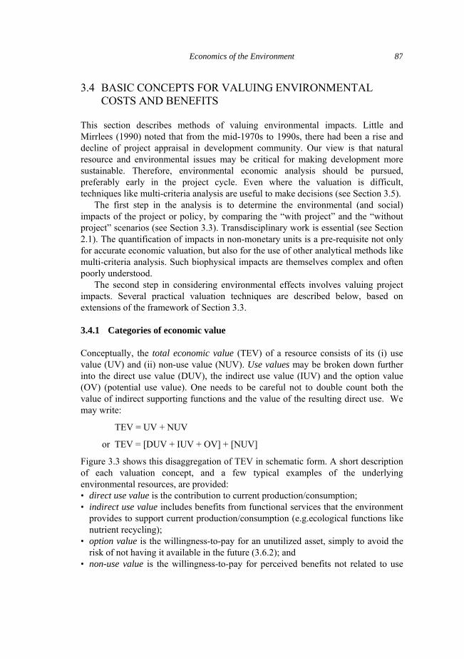
The second step in considering environmental effects involves valuing project impacts. Several practical valuation techniques are described below, based on extensions of the framework of Section 3.3. 3.4.1 Categories of economic value Conceptually, the total economic value (TEV) of a resource consists of its (i) use value (UV) and (ii) non-use value (NUV). Use values may be broken down further into the direct use value (DUV), the indirect use value (IUV) and the option value (OV) (potential use value). One needs to be careful not to double count both the value of indirect supporting functions and the value of the resulting direct use. We may write:

TEV = UV + NUV

or TEV = [DUV + IUV + OV] + [NUV]

Figure 3.3 shows this disaggregation of TEV in schematic form. A short description of each valuation concept, and a few typical examples of the underlying environmental resources, are provided: • direct use value is the contribution to current production/consumption; • indirect use value includes benefits from functional services that the environment

provides to support current production/consumption (e.g.ecological functions like nutrient recycling);

• option value is the willingness-to-pay for an unutilized asset, simply to avoid the risk of not having it available in the future (3.6.2); and

• non-use value is the willingness-to-pay for perceived benefits not related to use


88

value, e.g. existence value, which is based on the satisfaction of merely knowing that an asset exists, even without intending to use it.

Use Value Non-use Value

Total Economic Value

Direct use values Indirect use values

Option values Existence values Other non-use values

Outputs that can be consumed directly

Functional benefits

Future direct and indirect use values

Value from knowledge of continued existence

-Food-Biomass-Recreation-Health

-Ecological functions-Flood control-Storm protection

-Biodiversity-Conserved habitats

-Habitats-Endangered species

Decreasing tangibility of value to individuals

Use Value Non-use Value

Total Economic Value

Direct use values Indirect use values Option values Existence values Other non-use values

Outputs that can be consumed directly

Functional benefits

Future direct and indirect use values

Value from knowledge of continued existence

-Food-Biomass-Recreation-Health

-Ecological functions-Flood control-Storm protection

-Biodiversity-Conserved habitats

-Habitats-Endangered species

Decreasing tangibility of value to individuals

Figure 3.3 Categories of economic values attributed to environmental assets

(examples from a forest). Economic theory clearly defines TEV, but there is considerable overlap and ambiguity in the breakdown categories, especially with regard to non-use values. Thus, option values and non-use values are shaded in the figure. These categories are useful as an indicative guide, but the goal of practical estimation is to measure TEV rather than its components.

The distinction between use and non-use values is not always clear. The latter tend to be linked to more altruistic motives (Schechter and Freeman 1992). Differing forms of altruism include intergenerational altruism, or the bequest motive; interpersonal altruism or the gift motive; stewardship (which has more ethical than utilitarian origins); and q-Altruism, which states that the resource has an intrinsic right to exist. This final definition is outside conventional economic theory, and incorporates the notion that the welfare function should be derived from something more than purely human utility (Quiggin 1991).

For the practitioner, the precise conceptual basis of economic value is less important than the various empirical techniques that permit us to estimate a monetary value for environmental assets. 3.4.2 Practical valuation techniques The economic concept underlying all valuation methods is the willingness to pay (WTP) of individuals for an environmental service or resource, which is itself based


89

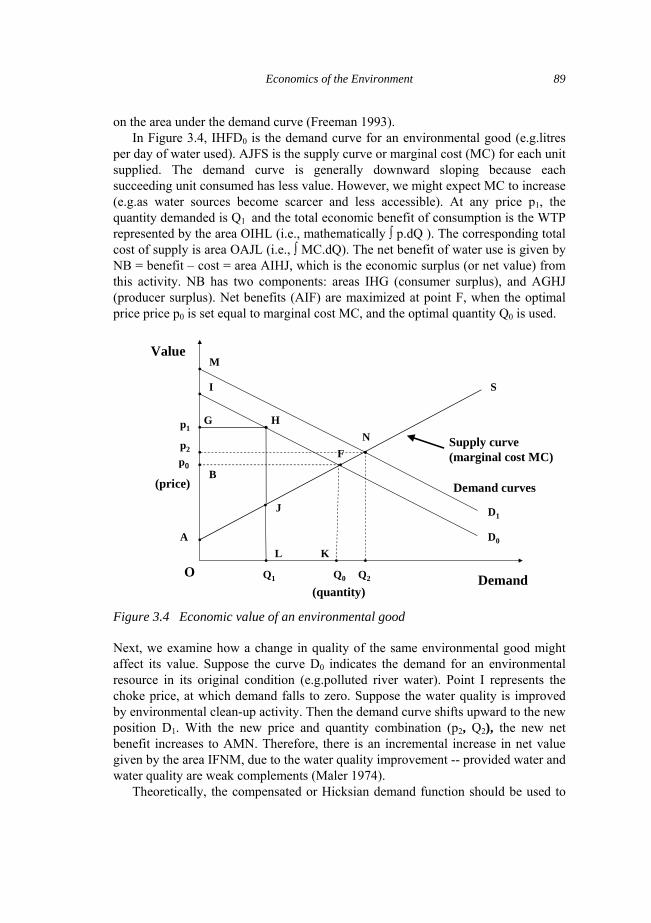
on the area under the demand curve (Freeman 1993). In Figure 3.4, IHFD0 is the demand curve for an environmental good (e.g.litres

per day of water used). AJFS is the supply curve or marginal cost (MC) for each unit supplied. The demand curve is generally downward sloping because each succeeding unit consumed has less value. However, we might expect MC to increase (e.g.as water sources become scarcer and less accessible). At any price p1, the quantity demanded is Q1 and the total economic benefit of consumption is the WTP represented by the area OIHL (i.e., mathematically ∫ p.dQ ). The corresponding total cost of supply is area OAJL (i.e., ∫ MC.dQ). The net benefit of water use is given by NB = benefit – cost = area AIHJ, which is the economic surplus (or net value) from this activity. NB has two components: areas IHG (consumer surplus), and AGHJ (producer surplus). Net benefits (AIF) are maximized at point F, when the optimal price price p0 is set equal to marginal cost MC, and the optimal quantity Q0 is used.

I

B

F

Q0 Demand

Value

D0

p0

O

Demand curves

A

S

Supply curve (marginal cost MC)

(price)

(quantity)

p2

Q2

D1

M

N

K

p1G H

J

L

Q1

Figure 3.4 Economic value of an environmental good Next, we examine how a change in quality of the same environmental good might affect its value. Suppose the curve D0 indicates the demand for an environmental resource in its original condition (e.g.polluted river water). Point I represents the choke price, at which demand falls to zero. Suppose the water quality is improved by environmental clean-up activity. Then the demand curve shifts upward to the new position D1. With the new price and quantity combination (p2, Q2), the new net benefit increases to AMN. Therefore, there is an incremental increase in net value given by the area IFNM, due to the water quality improvement -- provided water and water quality are weak complements (Maler 1974).

Theoretically, the compensated or Hicksian demand function should be used to


90

estimate value, since it indicates how demand varies with price while keeping the user's utility level constant. The change in value of an environmental asset could also be defined by the difference between the values of two expenditure (or cost) functions. The latter are the minimum amounts required to achieve a given level of household utility or firm output, before and after varying the quality of, price of, or access to the environmental resource, while keeping all other aspects constant.

Measurement problems arise because the commonly estimated demand function is the Marshallian one -- which indicates how demand varies with the price of an environmental good, while keeping the user's income level constant. In practice, it has been shown that the Marshallian and Hicksian estimates of WTP are in good agreement for a variety of conditions, and in a few cases the Hicksian function may be derived from the estimated Marshallian demand functions (Willig 1976, Braden and Kolstad 1991).

People’s willingness-to-accept (WTA) in the way of compensation for environmental damage is another measure of economic value that is related to the WTP; the WTA and the WTP could diverge as discussed below (Cropper and Oates 1992). In practice, both measures are used in the valuation techniques described below. Practical valuation methods are categorized in Figure 3.5.

Type of Market Behaviour Type

Conventional Market

Implicit Market

Constructed Market

Actual behaviour

Effect on production Effect on helath Defensive or preventive costs

Travel cost Wage differences Property values Proxy marketed goods

Artificial market

Intended behaviour

Replacement cost Shadow project

Benefit transfer Contingent valuation Choice Experiments

Source: Munasinghe (1992a)

Figure 3.5 Techniques for economically valuing environmental impact

Empirical evidence indicates that WTP questions yield higher answers than WTA questions about willingness to pay to retain the same amenity. Some argue that WTA questions need more time to be properly understood and assimilated, and that the gap between WTA and WTP narrows with successive iterations. Others suggest that people are less willing to pay actual income than to receive “hypothetical” compensation (Knetsch and Sinden, 1984). It may also be the case that individuals are more cautious when weighing the net benefits of changing assets than when no change is made. Generally, WTP is considered to be more consistent


91

and credible a measure than WTA. However, when significant discrepancies exist between the two measures, then the higher values may be more appropriate when valuing environmental losses.

In developing countries, the ability to pay is a concern. In low income areas, money values placed on environmental goods and services are traditionally low, and income weights may be used (see Section 3.2.2). Alternatively, other social and ethical measures might be used to protect the poor (see Section 13.2.3). Alternative measures such as willingness to give time to environmental-related activities (Ninan & Sathyapalan, 2005) are also gaining attention in the literature in addressing such concerns.

3.4.3 Direct effects valued on conventional markets The methods considered in this section are based on changes in market prices or productivity, due to environmental impacts.

Change in productivity. Projects can affect production. Changes in marketed output can be valued by using standard economic prices.

Loss of earnings. Environmental quality affects human health. Ideally, the monetary value of health impacts should be determined by the WTP for improved health. In practice, proxy measures like foregone net earnings may be used in case of premature death, sickness, or absenteeism (and higher medical expenditures, which can be considered a type of replacement cost). One may avoid ethical controversies associated with valuing a single specific life, by costing the statistical probability of ill-health or death (like the actuarial values used by life insurance firms).

Actual defensive or preventive expenditures. Individuals, firms, and governments undertake “defensive expenditures” to avoid or reduce unwanted environmental effects. Defensive expenditures may be easier to obtain than direct valuations of environmental harm. Such actual expenditures indicate that individuals, firms, or governments judge the resultant benefits to exceed the costs. Defensive expenditures can then be interpreted as a minimum valuation of benefits. 3.4.4 Potential expenditure valued on conventional markets

Replacement cost. Here, the costs to be incurred in order to replace a damaged asset are estimated. The actual damage costs may be higher or lower than the replacement cost. However, it is an appropriate method if there are compelling reasons for restoring the damage. This approach is especially relevant if there is a sustainability constraint that requires certain assets stocks to be maintained intact (see Chapter 2).

Shadow project. This approach is based on costing one or more “shadow projects” that provide for substitute environmental services to compensate for environmental assets lost under the ongoing project. Further, this approach is often


92

an institutional judgement of replacement cost, and its application would be most relevant when “critical” environmental assets at risk need to be maintained. 3.4.5 Valuation using implicit (or surrogate) markets Techniques described in this section use market information indirectly. Each method has advantages and disadvantages, including specific data and resource needs.

Travel cost. The travel cost method has been used to measure benefits produced by recreation sites. It determines the demand for a site (e.g.number of visits per year), as a function of variables like consumer income, price, and various socio-economic characteristics. The price is usually the sum of observed cost elements like a) entry price to the site; b) costs of travelling to the site; and c) foregone earnings or opportunity cost of time spent. The consumer surplus associated with the estimated demand curve provides a measure of the value of the recreational site in question. More sophisticated versions include comparisons across sites, where environmental quality is also included as a variable that affects demand.

Property value. This is a hedonic price technique based on the more general land value approach which decomposes real estate prices into components attributable to different characteristics like proximity to schools, shops, parks, etc. The method seeks to determine the increased WTP for improved local environmental quality, as reflected in housing prices in cleaner surroundings. It assumes a competitive housing market, and its demands on information and tools of statistical analysis are high.

Wage differential. This method is also a hedonic technique, which assumes a competitive market where the demand for labor equals the value of the marginal product and labour supply varies with working and living conditions. Thus, a higher wage is necessary to attract workers to locate in polluted areas or undertake more risky occupations. This method relies on private valuation of health risks, not necessarily social ones. Data on occupational hazards must be good for private individuals to make meaningful tradeoffs between health risks and remuneration. Finally, the effects of other factors like skill level, job responsibility, etc. that might influence wages must be eliminated, to isolate the impacts of environment.

Marketed goods as proxies for non-marketed goods. In situations where environmental goods have close substitutes that are marketed, the value of an environmental good may be approximated by the observed market price of its substitutes.

Benefit transfer. Values determined at one place and time are used to infer values of similar goods at another place and time (where direct valuation is difficult), with adjustments for differences in incomes, prices, quality, behaviour, etc. (ADB 1996, Ecological Economics 2006).


93

3.4.6 Valuation using constructed markets

Contingent valuation. When market prices do not exist, this method basically asks people what they are willing to pay for a benefit, and/or what they are willing to accept by way of compensation to tolerate a cost. This process of asking may be either through a direct questionnaire/ survey, or by experimental techniques in which subjects respond to stimuli in “laboratory” conditions. The contingent valuation method has certain shortcomings, including problems of designing, implementing, and interpreting questions. However, in some cases, it may be the only available technique for estimating benefits. It has been applied to common property resources, amenity resources with scenic, ecological or other characteristics, and to other situations where market information is not available. Caution should be exercised in seeking to pursue some of the more abstract benefits of environmental assets such as existence value.

Choice experiments (CE) are a recent valuation method based on Lancasterian consumer theory (Henscher, Rose & Greene, 2005). It is assumed that consumers make choices depending on preferences for a set of attributes of goods, rather than on simple marginal rates of substitution among goods. The CE takes place in a hypothetical setting, where individuals are asked to choose among alternatives in a choice set. Consumer choice is determined by the relative importance placed on various attributes of goods (e.g., price, appearance, etc.), during this process (Hanemann and Kanninen 1998).

Artificial market. Such markets could be constructed for experimental purposes, to determine consumer willingness to pay for a good or service. For example, a home water purification kit might be marketed at various price levels or access to a game reserve might be offered on the basis of different admission fees, thereby providing an estimate of the value placed on water purity or on the use of a recreational facility, respectively. 3.5 MULTI-CRITERIA ANALYSIS Projects, policies and their impacts are embedded in a system of broader (national) objectives. If the impacts of projects and policies on these broader objectives can be valued economically, all such effects may be incorporated into the conventional decisionmaking framework of cost-benefit analysis. However, some social and biophysical impacts cannot be easily quantified in monetary terms, and multi-criteria analysis offers a complementary approach, which facilitates decision making.

Multi-criteria analysis (MCA) or multi-objective decisionmaking differs from CBA in three major areas (van Pelt 1993). While CBA focuses on efficiency (although incorporation of income distribution objectives may be attempted), MCA does not impose limits on the forms of criteria, allowing for consideration of social and other forms of equity. Secondly, while CBA requires that effects be measured in quantitative terms, to allow for the application of prices, MCA can be broken down


94

into three groups: one that requires quantitative data, a second that uses only qualitative data, and a third that handles both simultaneously. Finally, MCA does not require the use of prices, although they might be used to arrive at a score. CBA uses prices which may sometimes be adjusted according to equity weighting. MCA uses weighting involving relative priorities of different groups as opposed to pricing. If efficiency is the only criterion and prices are available to value efficiency attributes, CBA is preferable. However, in many cases, a paucity of data, and the need to incorporate social and biophysical impacts makes the use of MCA a more practicable and realistic option.

MCA calls for desirable objectives to be specified. These often exhibit a hierarchical structure. The highest level represents the broad overall objectives (for example, improving the quality of life), often vaguely stated and, hence, not very operational. They may be broken down into more operational lower level objectives (e.g.increased income) so that the extent to which the latter are met may be practically assessed. Sometimes only proxies are available (e.g.if the objective is to enhance recreation opportunities, the number of recreation days can be used). Although value judgements may be required in choosing the proper attribute, measurement does not have to be in monetary terms (like the single-criterion CBA). More explicit recognition is given to the fact that a variety of concerns may be associated with planning decisions.

An intuitive understanding of the fundamentals of multi-criteria analysis can be provided by a two-dimensional graphical exposition such as in Figure 3.6. Assume that a scheme has two non-commensurable and conflicting objectives, Z1 and Z2. For example, Z1 could be the additional project cost required to protect biodiversity, and Z2, some index indicating the loss of biodiversity. Assume further that alternative projects or solutions to the problem (A, B and C) have been identified. Clearly, point B is superior (or dominates) to A in terms of both Z1 and Z2 because B exhibits lower costs as well as biodiversity loss relative to A. Thus, alternative A may be discarded. However, we cannot make such a simple choice between solutions B and C since the former is better than the latter with respect to objective Z1 but worse with respect to Z2. In general, more points (or solutions) such as B and C may be identified to define the set of all non-dominated feasible solution points that form an optimal trade-off curve or curve of best options.

For an unconstrained problem, further ranking of alternatives cannot be conducted without the introduction of value judgements. Specific information has to be elicited from the decisionmaker to determine the most preferred solution. In its most complete form such information may be summarized by a family of equi-preference curves that indicate the way in which the decision maker or society trades off one objective against the other -- typical equipreference curves are shown in Figure 3.6. The preferred alternative is the one that yields the greatest utility, which occurs (for continuous decision variables as shown here) at the point of tangency D of the best equi-preference curve, with the trade-off curve.

Since the equi-preference curves are usually not known other practical


95

techniques have been developed to narrow down the set of feasible choices on the trade-off curve. One approach uses limits on objectives or “exclusionary screening”. For example, in the figure, the decisionmaker may face an upper bound on costs CMAX (i.e., a budgetary constraint). Similarly, ecological experts might set a maximum value of biodiversity loss BMAX (e.g.a level beyond which the ecosystem collapses). These two constraints define a more restricted portion of the trade-off curve (darker line), thereby reducing and simplifying the choices available.

Source: Adapted from Munasinghe (1992a)

Figure 3.6 Simple multi-criteria analysis (MCA)

Pearce and Turner (1990) describe five main forms of multi criteria evaluation methods: aggregation, lexicographic, graphical, consensus-maximizing, and concordance. Among the various types of multi criteria analysis, the most suitable method depends upon the nature of the decision situation (Petry 1990). For instance, interactive involvement of the decisionmaker has proved useful for problems characterized by a large number of decision variables and complex causal interrelationships. Some objectives may be directly optimized, while others will need to meet a certain standard (e.g.level of biological oxygen demand (BOD) not below 5 mg/liter).


96

The major accomplishment of MCA models is that they allow for more accurate representation of decision problems, by accounting for several objectives. However, a key question concerns whose preferences are to be considered. The model only aids a single decisionmaker (or a homogeneous group). Various stakeholders will assign different priorities to the respective objectives, and it may not be possible to determine a single best solution via the multi objective model. Also, the mathematical framework imposes constraints upon the ability to effectively represent the planning problem. Non linear, stochastic, and dynamic formulations can assist in better defining the problem but impose costs in terms of complexity in formulation and solving the model (Cocklin 1989). In constructing the model the analyst communicates information about the nature of the problem by specifying why factors are important and how they interact. There is value to be gained in constructing models from differing perspectives and comparing the results Liebman (1976). MCA used in conjunction with a variety of models, and effective stakeholder consultations, could help to reconcile the differences between individual versus social, and selfish versus altruistic preferences.

In addition to facilitating specific tradeoff decisions at the project level, MCA could also help in selecting strategic development paths. 3.6 DISCOUNT RATE, RISK AND UNCERTAINTY In this section, some key issues that arise in the sustainable development assessment of projects and policies are briefly reviewed. 3.6.1 Discounting and inter-generational choices Discounting is the process by which costs and benefits that occur in different time periods may be compared. It has been a general problem in cost-benefit analysis, and is particularly important with regard to long term environmental issues (Harberger 1976, Marglin 1963).

In standard analysis, past costs and benefits are treated as “sunk” and are ignored in decisions about the present and future. Future costs and benefits are discounted to their equivalent present value and then compared. In theory the interest rate in a perfect market reflects both the subjective rate of time preference (of private individuals) and the rate of productivity of capital. These rates are equated at the margin by the market, so that the rate at which individuals are willing to trade present for future values is just equal at the margin to the rate at which they are able to transform present goods, in the form of foregone consumption, into future goods (through capital investment).

Often, the rate of time preference and the rate of capital productivity are not equal, because of imperfect financial markets and government distortions introduced by taxation. Also, individual decisions differ from social decisions in that individuals are relatively short-lived, whereas societies persist for longer periods.


97

The community usually discounts the future less than individuals. These considerations give rise to the concept of social rate of discount (see Box 3.2).

Box 3.2 Social rate of discount and long term concerns

Social rate of discount

The social rate of discount (SRD) is appropriate for determining public policy. Basic issues of value and equity are involved in the choice of such a social discount rate. Sustainable development provides a broad guideline -- each generation has the right to inherit a economic, social and environmental assets that are at least as good as the those enjoyed by the preceding generation (Chapter 2).

Even in traditional cost benefit analysis used in project evaluation, the choice of discount rates is not clear cut (Munasinghe 1992a). They vary across countries, depending on behavioural preferences and economic conditions. Furthermore, it is considered prudent to test the sensitivity of project results by using a range of discount rates (usually about 4 to 12 percent per annum), even within one country.

Starting from the theoretically ideal (or first best) situation of perfectly functioning, competitive markets and an optimal distribution of income (Box 2.3), it is possible to show that the discount rate should be equal to the marginal returns to investment (MRI) which will also equal the interest rate on borrowing by both consumers and producers (Lind 1982). There are three conditions to ensure an efficient (or optimal) growth path. First, the marginal returns to investment between one period and the next should equal the rate of interest (i) charged from borrowing producers. Second, the rate of change of the marginal utility of consumption (or satisfaction derived from one extra unit consumed) from one period to the next should be equal to the interest rate (r) paid out to lending consumers. Third and finally, the producer and consumer rates of interest are equal (i.e., i = r), throughout the economy and over all time periods.

As we deviate from ideal market conditions and the optimal income distribution, the choice of discount (or interest) rates becomes less clear. For example, taxes (subsidies) may increase (decrease) the borrowing rate to producers above (below) the interest rate paid to consumers on their savings (i.e., i differs from r). More generally, if the three conditions do not hold because of economic distortions, then efficiency may require project-specific discount rates with corrections to compensate for the economic imperfections. In some cases, no theoretical basis exists to link market interest rates to the social discount rate, but market behaviour could still provide useful data to estimate the latter.

Declining or negative discount rates (in the long term)

Traditional discount rate analysis may be used to derive declining (and even negative) discount rates for evaluating costs and benefits over very long (or multi-generational) time periods, when welfare and returns on investment may be falling. Consider the consumer rate of time preference (CTP), which is the subjective discount rate of individuals (as opposed to the MRI, which is market-derived). It has several components: CTP = α + βg. Here, α


98

represents the preference of an individual for consumption today rather than in the future -- it may be based on the myopic notion of “pure” preference, as well as the risk perception that future consumption may never be realized. β is the elasticity of marginal welfare and g is the growth rate of consumption.

Assuming that welfare (W) depends on consumption (c), we may write W = W(c). Then, by definition, β = −{c(d2W/dc2)/(dW/dc)} and g = (dc/dt)/c. Marginal welfare increases with consumption: (dW/dc) > 0; but at a declining rate: (d2W/dc2) < 0, as consumers become satiated. Therefore β > 0, so that the sign of the term (βg) is the same as sign of g. The term (βg) shows that the declining marginal welfare of consumption combined with higher expected future consumption will make the latter less valuable than present-day consumption, i.e., since we are likely to be richer in the future, consumption today is more valuable.

The general consensus is that α is close to zero, usually 0–3%, and β may be in the range of 1 to 2. Thus if g is large (i.e., high expected economic growth rates), then CTP could be quite large too. On the other hand, if we consider a long-range scenario in which growth and consumption are falling (e.g.catastrophic global warming in 100 years), then g could become negative and consequently CTP may be small or even negative. In this case, with CTP as the discount rate, future costs and benefits would loom much larger in present value terms than if the conventional opportunity cost of capital (say 8%) was used, thereby giving a larger weight to long-term, intergenerational concerns. The key point is that it may be misleading to choose discount rates without assuming some consistent future scenario: Uzawa (1969) shows how discount rates may be endogenized to reflect future consumption. Thus an optimistic future would favour higher discount rates than a gloomy one, which is consistent since the risk of future catastrophes should encourage greater concern for the future. Hansen (2006) and Winkler (2006) further discuss the pros and cons of declining (hyperbolic) discount rates.

Source: Munasinghe (1992a) The rate of productivity is higher in many developing countries, because of capital scarcity. In poor countries, the rate of time preference may also be elevated, because of the urgency of satisfying immediate basic needs rather than ensuring long-term sustainability.

The neoclassical discounted utility model implies that the rate of time preference is independent of time frames and the amounts of commodities -- this is not always true. Furthermore, the lack of properly developed capital markets in many developing economies often causes investment decisions to be linked to consumption, and to depend on preferences.

Higher discount rates may discriminate against future generations. This is because projects with social costs occurring in the long term and net social benefits occurring in the near term, will be favored by higher discount rates. Projects with benefits accruing in the long run will be less likely to be undertaken under high discount rates. Thus, future generations will suffer from market discount rates determined by high rates of current generation time preference and/or productivity of capital.


99

The foregoing arguments suggest that discount rates could be lowered to reflect long-term environmental concerns and issues of intergenerational equity – see Section 5.2.3 for a discussion relating to climate change. Yet, this may lead to a problem. Although ecologically sound activities would pass the cost-benefit test more frequently, many more projects would also generally pass the test, and the resulting increase in investment could lead to additional environmental stress. (Krautkraemer 1988).

Many environmentalists believe that a zero discount rate should be employed to protect future generations. However, employing a zero discount rate is inequitable, since it would imply a policy of high current sacrifice, which would discriminate against the poor of today. Non-constant (and declining) discount rates may be more relevant to deal with long term multi-generational issues (see Section 5.2.3), especially where the future productivity of capital is expected to decrease. The discount rate could be determined on a country-specific basis, and be regularly updated, as is the case with other shadow prices.

Arbitrary manipulation of discount rates to facilitate intergenerational transfers, could distort resource allocations. A better alternative might be to impose sustainability constraints to ensure that the overall stock of capital is preserved or enhanced for future generations (Chapter 2). Even simple rules that limit specific environmental impacts (e.g.pollution standards) may be a useful first step. Another alternative is to ensure that irreplaceable environmental assets command a premium value in CBA.

In summary, the following practical guidance is useful within the context of sustainomics: a) The standard opportunity cost of capital (e.g.range of 4-12 percent) may be used as a benchmark for NPV calculations, and as the comparator when the IRR is computed, b) Efforts should be made to ensure that compensating investments offset capital stock degradation within a framework of policy and project decisions; and c) In the case of projects leading to irreversible damage, CBA should be adapted to the extent possible, to include a measurement of the foregone benefits of preservation in the computation of costs; d) Where valuation of environmental and social impacts is difficult, and large irreversible damage might occur, restrictions might be set to limit the damage within acceptable biophysical or social norms; e) Declining or negative discount rates may be considered for pessimistic long term scenarios. 3.6.2 Risk and uncertainty problems All projects and policies entail risk and uncertainty. Risks are usually measured by the probabilities assigned to the likelihood of occurrence of an undesirable event (e.g.natural disaster). Uncertainty describes a situation where little is known about future impacts. Therefore, no probabilities can be assigned because the outcomes are undefined.

Risk can be treated probabilistically on the basis of estimated data, and therefore


100

insured against and treated like any other project cost. However, uncertainty defies actuarial principles because the future is undefined. As projects and environmental impacts grow larger, uncertainty looms larger than risk. The proper response to risk is to count it as a cost in expected value computations. However, the use of a single number (or expected value of risk) does not capture the risk variability or the range of values to be expected. Additionally, it does not allow for individual perceptions of risk. Precaution is one response to uncertainty -- if the future cannot be perceived clearly, then the speed of advance should be tailored to the distance over which the clarity of vision is acceptable.

In practice, the way risk and uncertainty are included in project appraisal work is through sensitivity analyses, which determine how the IRR is dependent on different variables. Using optimistic and pessimistic values for different variables can indicate which ones will significantly affect benefits and costs. Sensitivity analysis need not reflect the probability of occurrence of the upper or lower values. In project appraisal, deterministic point estimates of value could be quite misleading, whereas ranges of value help identify more robust options (Anderson and Quiggin 1990). Various criteria such as mini-max and minimum-regret also may be used (Friedman, 1986).

The issue of uncertainty plays an important role in environmental valuation and policy formulation. Option values and quasi-option values are based on the existence of uncertainty (see Section 3.4.1). Option value (OV) is essentially the premium that consumers are willing to pay to avoid the risk of not having something available in the future. Among the definitions of option value, one useful measure is the difference between the ex-ante and ex-post welfare associated with the use of an environmental asset. The sign of option value depends upon the presence of supply or demand uncertainty, and on whether the consumer is risk averse or risk loving (Pearce and Turner, 1990).

Quasi-option value (QOV) is the value of preserving options for future use in the expectation that knowledge will grow over time. If a project causes irreversible environmental damage, the opportunity to expand knowledge through scientific study of that asset is lost. Uncertainty about the benefits of preservation to be derived through future knowledge expansion (which is independent of development) yields a positive QOV. Thus development might be postponed until increased knowledge facilitates a more informed decision. If information growth itself depends on the development taking place, then QOV is positive when the uncertainty concerns preservation benefits, and negative when the uncertainty is about development benefits (Pearce and Turner 1990).

If calculations are performed in terms of the option price (valuing what a person would pay for future benefits today) then the option value may be redundant. The option value is added to expected future benefits to bring total value up to the option price. Most contingent valuation methods (CVMs) estimate the option price directly. Thus, OV may be practically redundant if it is captured in other measures, although conceptual valid (Freeman 1993).


101

Environmental policy formulation is complicated by the presence of numerous forms of uncertainty. As an illustration, Bromley (1989) identified six different aspects of uncertainty in the case of air pollution resulting from acid deposition. They are 1) identification of the sources of particular pollutants; 2) ultimate destination of particular emissions; 3) actual physical impacts at the point of destination; 4) human valuation of the realized impacts at the point of destination of the emissions; 5) the extent to which a particular policy response will have an impact on the abovementioned factors; and 6) the actual cost level and the incidence of those costs that are the result of policy choice.

Policymakers address these uncertainties based on their perception of the existing entitlement structure. The interests of the future may be protected by an entitlement structure that imposes a duty on current generations to consider the rights of future generations – since unborn generations are unable to enter bids in today’s markets, to protect their interests. There are three policy instruments to ensure that future generations are not made worse off: mandated pollution abatement; full compensation for future damages (e.g.by taxation); and an annuity that will compensate the future for costs imposed in the present. In the face of uncertainty, the first option would appear to be the most practical.

3.7 ECONOMYWIDE POLICIES AND THE ENVIRONMENT Next, we turn to larger scale issues that show how economywide policies (both macroeconomic and sectoral) may cause significant environmental and social harm. More details, including a historical review of ideas and recent case studies are given in Chapters 7, 8 and 9.

Fiscal and monetary policies, structural adjustment programs, and stabilization measures all effect the natural resource base. Unfortunately, interactions among the economy, society and environment are complex, and our understanding of them is limited. Ideally, one would wish to trace the effects of economywide policy reforms (both macroeconomic and sectoral) through the socio-economic and ecological systems. Time and data limitations generally preclude such comprehensive approaches in developing countries. Practical policy analysis is usually limited to a more partial approach which traces the key impacts of specific economywide policies, at least qualitatively, and wherever possible, quantitatively.

No simple generalizations are possible as to the likely environmental and social effects of broad policy measures. Nevertheless, opportunities have been missed for combining poverty reduction - or efficiency-oriented reforms with the complementary goal of environmental protection – i.e., “win-win” outcomes (Munasinghe 1992a). For example, addressing problems of land tenure as well as access to financial and social services not only yield economic gains but are also essential for promoting environmental stewardship. Similarly, improving the efficiency of industrial or energy related activities would reduce both economic waste and environmental pollution (World Bank 1992b-e).


102

Many instances of excessive pollution or resource over-exploitation are due to market distortions. Broad policy reforms, which usually promote efficiency or reduce poverty, could be made more beneficial for the environment. The challenge is to identify the complicated paths by which such policy changes ultimately influence conservation at the firm or household level. Some changes can have either beneficial or harmful environmental and social effects, depending on the nature of intervening conditions. The objective is not necessarily to directly modify the original broader policies (which have other conventional, non-environmental goals), but rather to design more specific complementary policy measures that would help mitigate negative effects or enhance the positive impacts of the original policies on the environment. 3.7.1 Macroeconomic policies During the economic crisis of the early 1980s, many developing countries that had been running substantial budget and trade deficits (and financing these by increasing external debt) were forced to adopt emergency stabilization programs. These programs often had unforeseen social and environmental consequences.

One important environmental impact of the crisis was related to poverty and unemployment. The stabilization efforts often necessitated currency devaluations, controls on capital, and interest rate increases. When income levels dropped, tax revenues decreased accordingly. As unemployment increased, governments fell back upon expansionary financing policies, which led to increases in consumer prices. The effect of such policies on the poorest population groups often drove them onto marginal lands, resulting in soil erosion or desertification. Fuel price increases and lowered incomes also contributed to deforestation and reductions in soil fertility, as the poor were forced to use fuelwood and animal dung for heating, lighting, and cooking.

Aside from the contractionary aspects of short-term stabilization measures, many macroeconomic policies also have potentially important effects on resource use and the environment. Unfortunately, no easy generalizations as to the directions of these effects are possible; they can be either beneficial or negative, depending on specific conditions. For example, real currency devaluations have the effect of increasing international competitiveness, and raising production of internationally tradable goods (for example, forestry and agricultural products). If the agricultural response occurs through crop substitution, environmental impact would depend on whether the crop being promoted tended to be environmentally benign (such as tea, cocoa, rubber) or environmentally damaging (such as tobacco, sugarcane, and corn). Environmental impacts would also depend on whether increased production led to farming on new land (which could result in increased deforestation) or to more efficient use of existing farmland. Another possibility is that overvaluation of the exchange rate (and resulting negative terms of trade, decreased competitiveness of products and lower farm gate prices), may well push small cultivators onto more


103

environmentally fragile marginal lands, in an attempt to absorb the effects of the price changes.

The output from a natural resource stock such as a forest or fishery will be affected by other factors like property rights (see Section 4.2). Thus, if trade policy increased the value of output (for example, timber or fish exports), then the degree of ownership would influence how production and resource stocks were managed. Reactions might range from more investment in and maintenance of assets (if environmental costs were internalized by owner-users) to rapid depletion (when the users had no stake in the resource stock). Thus, Capistrano and Kiker (1990) propose that increasing the competitiveness of world exports would also increase the opportunity cost of keeping timber unharvested. This could lead to forest depletion that significantly exceeds natural regenerative capacity. Another study (Kahn and McDonald 1991) used empirical evidence to suggest that a correlative link exists between debt and deforestation. They propose that debt burdens cause myopic behavior that often results in overdepletion of forest resources—through deforestation rates that may not be optimal in the long run, but are necessary to meet short-term needs.

Munasinghe and Cruz (1994) explicitly traced how economywide policy reforms to promote economic development could have numerous unanticipated environmental and social effects. Table 3.1 summarizes some typical results. Table 3.1 Typical examples of direct and indirect environmental and social impacts

of economywide policies

Policy Issue

Policy Reform

Direct Economic Objectives/ Effects

Indirect (Environmental and Social Effects)

1. Trade deficits

Flexible exchange rates.

Promote industrial competitiveness, exports; reduce imports.

Export promotion might promote more deforestation for export, and lead to substitution of tree crops for annual crops. Industrial job creation may reduce pressure on land resources.

2. Food security and unemployment

Agricultural intensification in settled lands and resettlement programs for new areas.

Increase crop yields and acreage; absorb more rural labor.

May reduce spontaneous migration to ecologically fragil areas. However there is potential for overuse of fertilizers and chemicals.

3. Industrial protection, due to inefficient production.

Reduce tariffs and special investment incentives.

Promote competition and industrial efficiency.

More openness may lead to more energy-efficient or less polluting technologies. It may also attract hazardous industries.

The first column lists only a few of the many economywide policy issues

addressed through macroeconomic reforms. The policies in the second column of the table are usually designed to address these issues, with the corresponding economic development objectives or direct impacts in the third column. The fourth


104

column shows important second-order environmental and social impacts that may not be anticipated. While policy reforms could improve natural resource management, some potential negative environmental impacts that concern us are given in this column. Thus, to properly evaluate such reforms, it would be necessary to assess their direct and indirect effects as well as the trade-offs between their conventional development contribution and their environmental effects. Relevant defensive measures or modifications may then be analyzed for each policy. This systematic process is captured in the Action Impact Matrix (AIM) methodology (see Section 2.4.1).

The key influence of macroeconomic policies on agriculture has already been shown by early studies (Johnson l973, Schuh l974). Krueger, Schiff, and Valdes (l99l) also show that economywide factors may be more important than sectoral policies in agriculture. When a broad assessment perspective is adopted, direct output price interventions by government have less effect on agricultural incentives than indirect, economywide factors, such as foreign exchange rates and industrial protection policies.

The impact of economywide policies may also be important for the environment. For example, Hyde et al. (l99l) cite studies in Brazil and in the Philippines that demonstrate how economic policy spillovers constitute an important source of deforestation. Agricultural subsidies in Brazil probably contribute to half of forest destruction in Amazonia (Mahar l988, Binswanger l989). A general equilibrium simulation for the Philippines suggests that foreign exchange rate changes, although motivated by general balance of payments concerns, have major implications for the demand for wood products, therefore influencing logging rates. The case of fuelwood may be as interesting, since fuelwood shortages have been identified as the major forestry problem in many developing countries. National price policies on fuel and investment policies on alternative energy sources may be important for addressing the fuelwood problem. 3.7.2 Structural adjustment Structural adjustment programs address a well-defined set of reform areas (see Section 7.2.1). These will generally include establishing an appropriate macroeconomic framework for growth, introducing a set of supporting sectoral policies and investment efforts, and integrating the domestic economy into the world economy (Fischer and Thomas l990).

Adjustment lending in the early l980s addressed problems of maintaining growth caused by the worldwide economic crisis. The crisis was triggered by the second round of energy price hikes, the collapse of export markets, and increased international interest rates. These external conditions, combined with lack of competitiveness of local industries, lagging employment generation, and persistent budget deficits, led to unsustainable current account deficits.

Thus, trade-oriented reforms, including tariff reductions and devaluation, became


105

key components of adjustment lending. Adjustment implications for managing external debt also received much attention. In turn, this led to concerns for stimulating domestic savings, increasing the role of taxation in resource mobilization, decreasing the extent of government expenditures, and making investments more productive.

The benefits and costs of such programs are country-specific. In a review of the Latin American experience, Birdsall and Wheeler (1992) conclude that there is no evidence to show that open developing country economies are more prone to pollution. The inflow of foreign technology and capital would tend to bring in better pollution standards. At the same time, it is the pollution-intensive heavy industries sector that has benefited from protective industrial and trade policies. Nevertheless, some concern persists that encouraging foreign investment and privatization might lead to the growth of “pollution havens,” given the weakness of environmental regulations in most developing countries. Trade liberalization also could encourage the growth of energy-intensive and/or highly polluting industry. However, pollution caused by industrialization could be offset by afforestation (although this does not necessarily compensate residents of polluted areas), and limited by appropriate taxation policies that encouraged the use of pollution abatement technologies.

The environmental relevance of structural adjustment reforms was reviewed (Warford et al. 1992). The reforms included (l) relative price changes in agricultural outputs, inputs, energy, export taxes; (2) trade and industry policy reform; (3) changes in public expenditure programs; and (4) institutional reforms by sector. In the early to mid-l980s, environmental aspects were relatively neglected in adjustment lending operations, with few environmental loan components or conditionalities. The review also found that programs from FY88-FY92, included more on the environment. For example, about 60% of the 58 countries reviewed had adjustment programs whose loan components or conditionalities were environmentally related, compared to 37% during FY79-FY87. Sectoral adjustment programs have also included environmental policy reforms.

In the 1990s, international donor agencies, non-governmental organizations and academic institutions contributed to the debate on the environmental effects of structural adjustment and stabilization programs. Several good studies of environmental and social impacts of countrywide policies exisit (Munasinghe 1992a, Reed 1992; Munasinghe and Cruz 1994; Abaza 1995; Young and Bishop 1995; Munasinghe 1996; Reed 1996; Opschoor and Jongma 1996; Panayotou and Hupe 1996; Cruz, Munasinghe and Warford 1997; Warford, Munasinghe and Cruz 1997; Kessler and Van Dorp 1998; and Environment and Development Economics 1999) – see Chapter 7 for details. 3.7.3 Public investment/expenditure reviews Reductions in public expenditure are an integral part of many structural adjustment loans, and usually emerge from recommendations on spending priorities made in


106

Public Investment/Expenditure Reviews (PI/ERs). The main purpose of PI/ERs is to provide recommendations to governments on the size and composition of their spending programs and on ways to strengthen local institutions in ways that enhance country capabilities to design and implement such programs. They have also been used to carry out basic sector work and to identify projects appropriate for World Bank support. PI/ERs facilitate expenditure decisions by the core planning and finance agencies, which are central to the key objectives of structural adjustment, poverty alleviation, and sound management of natural resources.

Public investment programs often do not give adequate weight to environmental objectives as compared to efficiency and poverty alleviation. The potential exists for investment reviews to appropriately elevate environmental concerns and thereby help to avoid making investments that have some of the serious long-term environmental consequences. While the expenditure reviews are perhaps less crucial, these could be used to ensure, for example, that environmental agencies and their programs get a fair share of current government expenditures. 3.7.4 Sectoral policies While adjustment is inherently a macroeconomic effort, involving macroeconomic policy reform, it also requires specific sectoral reforms (Munasinghe and Cruz 1994). The key macroeconomic variables in adjustment programs are the investment-savings gap, the fiscal deficit, the trade deficit, the exchange rate, and the rate of inflation. The microeconomic or sectoral reforms relevant to adjustment include industrial promotion and investment incentives, tax incidence, import liberalization and trade, and energy pricing. These are undertaken to improve resource allocation, but they also have important implications for macroeconomic stability and growth (Fischer and Thomas l990). The first is primarily a microeconomic goal while the second is an adjustment goal.

For example, taxation and government expenditures are the prime microeconomic mechanisms for resource allocation. However, they also comprise the basic elements of fiscal policy. In turn, fiscal policy has a critical macroeconomic impact because it directly determines the fiscal deficit and therefore affects the current account deficit and, after a lag, investment levels. Tax reform issues are particularly relevant from an environmental management perspective because they can have a wide range of potential impacts on resource use. The choice of the tax or tariff base can lead to substantial changes in the level of pollution-related activities. However, such environmental implications are not considered in conventional assessments that focus on fiscal effectiveness. Other sectoral reforms, such as those dealing with energy pricing and industrial exports, also affect macroeconomic stability and have thus played a regular role in adjustment programs (World Bank l989).

Beyond their role in contributing to a stable macroeconomic environment, sectoral policies also have economy-wide relevance in terms of promoting growth


107

from the supply side. These include sectoral investment and pricing policies as well as sectoral regulation and institutional development. As noted by Fischer and Thomas (l990), the traditional approach to development was through investment in agriculture, industry, infrastructure, and human resources. However, the contribution of these sectoral investments also depended largely on macroeconomic policies and the presence of enabling institutions. Some countries subsidize urban consumers by placing price ceilings on food. In such cases, the environmental consequences will be the same as for currency overvaluation, as both results in lowered incentives to increase production of internationally tradable crops.

In the case of Brazil, Binswanger (1989) showed that general tax policies, special tax incentives, the rules of land allocation, and the agricultural credit system all accelerate deforestation in the Amazon. These policies also increase landholding size and reduce the land available to the poor. Mahar (1989) traced many problems in the Amazon in Brazil to the decision in the mid-1960s to provide overland access to Amazonia. Further examples of sectoral work that address issues of environmental concern through economywide policy reform are given in Chapter 7, Munasinghe and Cruz (1994), and Munasinghe (1997). 3.7.5. National income accounts and macroeconomic performance In order to accurately recognize and include environmental concerns in macro-economic analyses, standard national income accounting techniques must be re-examined. Performance is currently measured by the growth in gross domestic product (GDP), and policy reforms are justified routinely on the basis of their short-, medium-, or long-term contribution to such growth. While GDP measures market activity reasonably well, it has been criticized for its neglect of other key aspects such as non-market value added, income distribution, and so on. Further, GDP does not consider depreciation of manmade capital (although the less quoted net domestic product or NDP does), and also leaves out the degradation of “natural capital.” Thus, GDP is an inaccurate measure of true, sustainable income.

In terms of the environment, there are several shortcomings in the widely used traditional system of national accounts (SNA) framework: 1. Natural and environmental resources are not fully included in balance sheets;

therefore, national accounts represent limited indicators of national well-being, since they are a poor, or even “perverse,” measure of changes in environmental and natural resource conditions;

2. Conventional national accounts fail to record the true costs of using natural resources in economic activity. The depletion or degradation of natural capital stocks (water, soil, air, minerals, and wilderness areas), which occurs due to productive activity is not included in current costs or depreciation of natural wealth. Thus, resource-based goods are underpriced -- the lower the value added, the larger is the extent of underpricing of the final product. Some countries promote primary product exports by subsidizing them, often with


108

disproportionately large adverse impacts on the poor (who are less able to protect themselves) -- the small cultivator, the forest dweller, landless peasant, and so on. If such hidden costs or “subsidies” were estimated, the GDP of many countries could well be significantly lower. In addition, natural resource depletion raises intergenerational equity issues, since productive assets available to future generations may be unfairly diminished (see Section 3.6.1).

3. Cleanup or abatement activities (e.g.expenditures incurred to restore environmental assets) often serve to inflate national income, while the offsetting environmental damages are not considered. For private firms, defensive environmental expenditures are netted out of final value added. In contrast, such cleanup costs are considered as productive contributions to national output if they are incurred by the public sector or households. GDP calculations are distorted in two ways, because undesirable outputs (like pollution) are overlooked while beneficial environment-related activities are often implicitly valued at zero.

Such deficiencies in the accounting techniques employed up to the 1980s pointed to the need for a system of national accounts (SNA) which permits the computation of an environmentally adjusted net domestic product (EDP) and an environmentally adjusted net income (EDI). National level decision makers and macroeconomic planners (typically, in a Ministry of Finance or Planning) routinely rely on the conventional SNA to formulate economic policies. Thus, a supplementary environmentally adjusted SNA and corresponding performance indicators would encourage policymakers to reassess the macroeconomic situation in light of environmental concerns and to trace the links between economywide policies and natural resource management (Munasinghe and Cruz 1994).

Based on work done during the 1980s (Bartelmus, Stahmer, and van Tongeren 1989), the System for Environmentally-adjusted Economic Accounts (SEEA) was created as an interim measure. Its objective was to integrate environmental data sets with existing national accounts information, while maintaining SNA concepts and principles insofar as possible. Environmental costs, benefits, and natural resource assets, as well as expenditures for environmental protection, were presented as satellite accounts in a manner consistent with the accounting framework of the SNA. The method involved disaggregation of the conventional SNA to highlight environmental relationships, linked physical and monetary accounting, imputations of environmental costs, and extensions of the SNA production boundary – without modifying the core accounts.

The SEEA framework received further impetus through the UN interim handbook on environmental accounting (UN, 1993), which outlined the possibilities for computing various national accounts aggregates such as ‘green GNP’ – that are adjusted downward to reflect the costs of net resource depletion and environmental pollution. Green net national product is a Hicks-Lindahl measure of potentially sustainable income (Hicks, 1946). However, it cannot indicate whether the saving


109

rate can maintain this income indefinitely, and typically does not measure potential consumption if the economy were actually on a constant-utility path. ‘Genuine savings’ is a better measure of macro-sustainability (Atkinson et al., 1997). Further work is outlined in Section 7.1.5.

Next, an operational handbook was published (UN 2000), and finally the Integrated Environmental and Economic Accounting Handbook was issued in 2003 (UN 2003). The revisions provide methods to estimate environmental and natural resource related expenditures, which were not effectively captured in conventional SNA. Features include: (1) natural resource asset accounts which include natural resource stock depletion, and improve the balance sheets of the conventional SNA; (2) pollutant and material flow accounts which report the use of energy and materials, and the generation of pollutants and wastes in the production process and the final demand. These accounts are linked to the supply and use tables of the IO table described in SNA; (3) environmental protection and resource management expenditures are shown more explicitly and this data may be used for policy analysis and other research on sustainable development; and (4) better macroeconomic aggregates like environmentally adjusted Net Domestic Product have been developed.

Natural resource accounts have a balance sheet flavour, with their emphasis on opening and closing stocks in quantity and values of natural resources, including both commercial natural resources and non-commercial or environmental resources. Thus, resource accounts underlie the expanded national balance sheet accounts in the revised SNA. The principal policy and analytical uses of these accounts include: measuring physical scarcity, resource management, assessing the balance sheet of the resource sectors, productivity measurement, portfolio analysis and management, valuing depletion, and identifying effects of environmental degradation. Natural resource accounts, and their counterparts in the national balance sheet accounts, can therefore have wide use with regard to resource management policies and broader environmental policies.

Several countries have explored various environmental adjustments to the SNA (World Bank 2006). Various measures of national product and wealth are under consideration, including natural resource (stock) accounts, resource and pollutant flow accounts, environmental expenditure accounts, and alternative national accounts aggregates (Atkinson et al. 1997). However, no countries have formally altered their SNA to reflect the environmental concerns in the 2003 revision to the SNA (UN 2003), although pilot studies have been done.

The simple measure introduced in Section 2.3.5 to indicate the sustainability of natural resource stocks may be extended to cover total wealth per capita. The latter would be a useful indicator of sustainability, if the SNA aimed to measure total national wealth (including the value of stocks of manufactured capital, as well as living and non-living resources). For total wealth W and population P, development is (weakly) sustainable, when:

S = [d(W/P)/dt]/[W/P] ≥ 0


110

This index has several desirable properties -- e.g.separately accounting for changes in natural assets having low substitution possibilities. Evolution of practical applications

The World Bank, together with the UN Statistical Office (UNSO), completed early case studies in Mexico (van Tongeren et al. 1991), and Papua New Guinea (Bartelmus et al. 1991), to determine how such accounts can be prepared. The Papua New Guinea study demonstrates the feasibility of applying the SEEA framework in a country with relatively weak institutional capacities and limited data availability, (a scenario that would exist in many resource-rich developing countries). Depreciation of produced assets was calculated to be 9-11 percent of Gross Domestic Product (GDP), resulting in a conventional Net Domestic Product (NDP) of between 89 and 91 percent of GDP. Environmental impacts were assessed for the agriculture, forestry, mining and energy sectors.

The authors estimated that these impacts were about 2 percent of NDP on average, for the 1986-1990 time period. First, the Environmentally—adjusted net Domestic Product 1 (EDP 1) was calculated, which incorporates the “economic” depletion costs of natural resource use, (but does not account for the degradation of environmental quality and corresponding losses of non-marketed environmental services that is reflected in EDP2). Next, EDP2 was estimated after subtracting the costs of degradation of environmental quality from EDP1. EDP2 was estimated to range from 90 to 97 percent of NDP. The final results showed that consumption exceeded net environmentally adjusted domestic production in most years. However, lack of physical data made it extremely difficult to obtain accurate estimates. Significant fluctuations in commodity prices also reflect the difficulties for governments in attempting to maintain sustainable development policies.

Additionally, contrary to findings, Papua New Guinea is not necessarily depleting its capital base, as the capital gain from erosion of external debt (caused by inflation reducing the value of the debt) is about 4% of GNP in real terms. The substitutability of capital is therefore an issue to be considered in the definition of “income”. In addition to these World Bank-supported studies, a few examples exist of the application of environmental accounting in developing countries (and even less in the developed world). The UN Economic Commission for Latin America and the Environment (ECLAC) and UNEP performed two case studies in Latin America that apply environmental accounting methodologies to limited areas within countries (CIDIE 1992). The Argentina study valued a forest ecosystem by estimating the costs of improving productive functions and of maintaining ecosystem functions. Results gained were employed in modelling alternative management and exploitation scenarios. The Mexico study calculated adjustments to the gross product, due to a biological corridor, using market valuation of replacement cost in the agricultural and forestry sectors, and constructed physical balance sheets for individual resources. The Hicksian concept of income was utilized to provide a revised measure of the region's income.


111

Gilbert (CIDIE 1992) did a study of Botswana using an environmental accounting framework within a larger modelling and information system. The approach used stock accounts (describing natural resource stocks in physical units); resource user accounts (describing stocks in physical and monetary units); and socio-economic accounts (focusing on resource use, demographics, and environmental policy). However, full implementation of the framework has not been possible because of severe data constraints.

An early application of environmental accounting in a developing country was performed by Repetto et al. (1989) for the World Resources Institute. The study collected data on petroleum, timber, and soil resources. The approach used is based upon physical stock and flow accounts of natural resources, and the valuation of these stocks. It has been suggested that the valuation method used in forestry overestimates the true resource depreciation, but has nevertheless proved extremely useful as an indicator of the magnitudes involved in adjustments to GDP through environmental accounting (CIDIE 1992). A later study (WRI 1991) utilized the same valuation methodology for forestry, but focused on providing detailed methods for the technical estimates of deforestation, soil erosion, and coastal fishery over-exploitation in Costa Rica.

Recent work suggests that Bolivia may be on an unsustainable development path (World Bank, 2006). When depletion of natural resources is included, the genuine national savings rate became minus 3.8% of gross national income (GNI) in 2003, although the traditionally computed national savings rate was 12% of GNI. In this estimate, depletion of energy, metals, and minerals was 9% percent of GNI and pollution damage was almost 7%, while the net forest depletion was zero.

Some researchers have computed more composite indices of human welfare to show that the relationship between ‘true’ welfare and conventional income per capita is positive in the early development stage but becomes negative later -- in contrast to the EKC effect (Daly and Cobb 1990, Max-Neef 1995). One such measure called Index of Sustainable Economic Welfare (ISEW), has already peaked in the 1970s or 1980s and is now declining for the US, UK, Germany, Austria and Netherlands. Poverty alleviation remains a dominant social objective (Sen 1984). Lawn (2005) examines the valuation methods used to calculate the Index of Sustainable Economic Welfare, the Genuine Progress Indicator, and the Sustainable Net Benefit Index. He argues that a consistent and more robust set of valuation techniques is required in order for these alternative indexes to gain broad acceptability as a means of comparing the costs and benefits of growth. Recent work seeks to expand the social accounting matrix (SAM) to include the distributional impacts of environmental damage across income groups (Munasinghe 2002).


112

Annex 3.1. Estimating and Using Shadow Prices

Numeraire

To derive a consistent set of economic shadow prices for goods and services, a common yardstick or numeraire to measure value is necessary. The same nominal unit of currency may have a different value depending on the economic circumstances in which it is used. For example, a rupee-worth of chocolate purchased in a duty free shop is likely to be more than quantity of chcoclate obtained for one rupee from a retail store (after import duties and taxes have been levied). Therefore, it is possible to distinguish intuitively between the border-priced rupee, which is used in international markets free of import tariffs, and a domestic-priced rupee, which is used in the domestic market subject to various distortions.

The choice of the numeraire, like the choice of a currency unit, should not change the outcome of an economic decision – provided the same consistent framework and assumptions are used in the analysis. For example, only one difference exists between a cost-benefit study which uses “cents” as units, and another which uses “rupees” (one rupee is equal to 100 cents). In the analysis using cents, all quantities will be numerically one hundred times larger than in the one using rupees. Since the analytical results will not be changed by this linear scale factor, one may choose the numeraire according to convenience.

A most appropriate numeraire in many instances is a unit of uncommitted public income at border shadow prices (Little and Mirrlees 1974). This unit is the same as freely disposable foreign exchange available to the government, but expressed in terms of units of local currency converted at the official exchange rate (OER). The border-priced numeraire is particularly relevant for the foreign exchange-scarce developing countries. It represents the set of opportunities available to a country to purchase goods and services on the international market. Economic efficiency shadow prices

The estimation and use of efficiency shadow prices is facilitated by dividing economic resources into tradeable and nontradeable items. Tradeables are directly imported or exported goods and services, and their values are already known in border prices – i.e., foreign exchange costs converted at the OER. Nontradeables are local goods whose values are known only in terms of domestic market prices, which must be converted to border prices, by applying conversion factors (CF).

Border (Shadow) Price = Conversion Factor x Domestic(Market) Price

BP = CF x DP

For tradeables with infinite elasticities (of world supply for imports and world demand for exports), the cost, insurance, and freight (C.I.F.) border price for imports and the free-on-board (F.O.B.) border price for exports may be used (with a suitable adjustment for the marketing margin). If the relevant elasticities are finite, then the


113

change in import or export costs, as well as any shifts in other domestic consumption or production levels or in income transfers, should be considered. The free trade assumption is not required to justify the use of border prices since domestic price distortions are adjusted by netting out all taxes, duties, and subsidies.

To clarify this point, consider a household where a child is given an allowance of twenty pesos a month as pocket money. The youngster may purchase a bag of sweets from a store at a price of two pesos. If the parents want to discourage consumption of sweets, they may impose a fine of one peso on each bag. The fine is exactly like an import duty, and the child must surrender three pesos for every bag of candy (valued at its domestic price, inside the household). From the family’s perspective, the total external payment for the item is only two pesos, because the one peso fine is a net transfer within the household. Therefore, the true economic cost (or shadow price) of the bag of lollipops to the household is two pesos (i.e., its border price), when the impact of the fine on the distribution of the income between parent and child is ignored.

A nontradeable is conventionally defined as a commodity whose domestic supply price lies between the F.O.B. export price and C.I.F. import price. Items that are not traded at the margin because of prohibitive trade barriers, such as bans or rigid quotas, are also included within this category. If the increased demand for a given nontradeable good or service is met by the expansion of domestic supply or imports, the associated border-priced marginal social cost (MSC) of this increased supply is the relevant resource cost. If decreased consumption of other domestic or foreign users results, the border-priced marginal social benefit (MSB) of this foregone domestic consumption or of reduced export earnings, would be a more appropriate measure of social costs.

The socially optimal level of total consumption for the given input (Qopt) lies at the point where the curves of MSC and MSB intersect. Price and non-price distortions lead to nonoptimal levels of consumption Q ≠ Qopt , where MSB ≠ MSC. More generally, if both effects are present, a weighted average of MSC and MSB should be used. The MSB is more important in a short-run, supply constrained situation, while the MSC dominates in the longer run, when expansion of output is possible.

The MSC of nontradeable goods and services from many sectors can be determined through appropriate decomposition. For example, suppose one peso-worth, of the output of the construction sector (valued in domestic prices), may be broken down successively into components -- like capital, labor, materials, etc., which are valued at pesos C1, C2,… Cn in border prices. Then the construction conversion factor (defined as the ratio of the border price to the domestic price), is given by:

n CCF = ∑ Ci

i = 1


114

The standard conversion factor (SCF) may be used with nontradeables that are not important enough to merit individual attention, or lack sufficient data. The SCF is equal to the OER divided by the more familiar shadow exchange rate (SER), appropriately defined. Using the SCF to convert domestic priced values into border price equivalents, is conceptually the inverse of the traditional practice of multiplying foreign currency costs by the SER (instead of the OER), to convert foreign exchange to the domestic price equivalent. The SCF is approximated by the ratio of the official exchange rate to the free trade exchange rate (FTER), when the country is moving toward a freer trade regime:

SCF = )tnM(1)teX(1

nMeXFTEROER

mx ++−+

=

where, X = F.O.B. value of exports, M = C.I.F. value of imports, e = elasticity of domestic supply of exports, n = elasticity of domestic demand for imports, tx = average tax rate on exports (negative for subsidy), and tm = average tax rate on imports.

The foregone output of workers is the dominant component of the shadow wage rate (SWR). Consider unskilled labor in a labor surplus country -- for example, rural workers employed in an urban factory. Complications arise in estimating the opportunity cost of labor, because the original rural income earned may not reflect the marginal product of agricultural labor. Furthermore, for every new urban job created, more than one rural worker may give up former employment. Adjustments are also needed for seasonal activities such as harvesting, and overhead costs like transport expenses. Then, the efficiency shadow wage rate (ESWR) is given by:

ESWR = a.m + c.u,

where m and u are the foregone marginal output and overhead costs of labor in domestic prices, and a and c are corresponding conversion factors to convert these values into border prices.

The appropriate shadow value placed on land depends on its location. Usually, the market price of urban land is a good indicator of its economic value in domestic prices, and the application of an appropriate conversion factor (such as the SCF) to this domestic price, will yield the border-priced cost of urban land inputs. Rural land that can be used in agriculture may be valued at its opportunity costs -- the net benefit of foregone agricultural output. The marginal social cost of other rural land depends on potential uses like recreation (see Section 3.4).

The shadow price of a capital is usually reflected in the discount rate or accounting rate of interest (ARI), which is defined as the rate of decline in the value of the numeraire over time (see Sections 3.2 and 3.6). In terms of pure efficiency, one practical proxy for ARI is the opportunity cost of capital (OCC) -- defined as the expected value of the annual stream of consumption, in border prices net of


115

replacement, which is yielded by the investment of one unit of public income at the margin. Adjustments for social (and environmental) shadow prices

If social pricing is important, it is necessary to include the effect of changes on consumption patterns. Starting with the efficiency shadow wage rate (ESWR), suppose a worker receives a wage Wn in a new job, and that the income forgone is Wo (both in domestic prices). We note that Wn may not necessarily be equal to the marginal product foregone m. It could be assumed, quite plausibly, that low-income workers consume the entire increase in income (Wn - Wo). Then this increase in consumption will result in a resource cost to the economy of b(Wn - Wo). The increased consumption also provides a benefit given by w(Wn - Wo), where w represents the MSB, in border prices, of increasing domestic-priced private sector consumption by one unit.

Thus, we may estimate the following social shadow wage rate (adjusted for consumption effects):

SSWR = a.m + c.u + (b - w) (Wn - Wo)

Here b represents the MSC, of increased consumption. If all new income is consumed, then b is the consumption conversion factor or resource cost (in units of the numeraire) of supplying consumers with one unit worth (in domestic prices) of the marginal basket of goods they would purchase.

n b = ∑ gi .CFi

i =1

where, gi is the proportion or share of the i th good in the marginal consumption basket, and CFi is the corresponding conversion factor.

The corresponding MSB of increased consumption is given by: w = d/v. Here, 1/v is the value (in units of the numeraire) of a one-unit increase in domestic-priced consumption accruing to someone at the average level of consumption (ca). Therefore, v may be roughly thought of as the premium attached to public savings, compared to “average” private consumption. Under certain simplifying assumptions, b = 1/v.

d is a form of “social weighting” which favours the poor. If MU(c) denotes the marginal utility of consumption at some level c, then d = MU(c) / MU(ca). Assuming that the marginal utility of consumption is diminishing, d would be greater than unity for “poor” consumers who are below the average level of income (i.e., c < ca), and vice versa. A simple form of marginal utility function could be: MU(c) = c-n. Thus, d = MU(c) / MU(ca) = n(ca/c). Making the further assumption that the distribution parameter n = 1, gives:

d = ca/c = ia/i ;


116

where ia/i is the ratio of net incomes, which may be used as a proxy for the corresponding consumption ratio. In this simple case, the social weight d is equal to the income ratio.

The consumption term (b-w) in the expression for SSWR disappears if, at the margin: (a) society is indifferent to the distribution of income (or consumption), so that everyone’s consumption has equivalent value (d = 1); and (b) private consumption is considered to be as socially valuable as uncommitted public savings (b = 1/v).

A simple formula for the social shadow price of capital, which also includes consumption effects, is given by:

SARI = OCC [s + (1 – s)w/b],

where, s is the fraction of the yield from the original investment that will be saved and reinvested.

Adjustments for environmental shadow prices are based on environmental externalities (see Section 3.4). Since the rigorous estimation of shadow prices is a long and complex task, it is advisable to use whatever shadow prices have already been calculated. Alternatively, one might estimate a few important items such as the standard conversion factor, opportunity cost of capital, and shadow wage rate. When the data are not precise enough, sensitivity studies may be made over a range of values of such key national parameters.

chapter 3 - mohan munasinghe

Documents