chapter 4 pv-upqc based harmonics...
TRANSCRIPT

66
CHAPTER 4
PV-UPQC BASED HARMONICS REDUCTION IN POWER
DISTRIBUTION SYSTEMS
INTRODUCTION
The use of electronic controllers in the electric power supply system
has become very common. These electronic controllers behave as nonlinear
load and cause serious distortion in the distribution system and introduce
unwanted harmonics in the system, leading to decreased efficiency of the
power system network and equipment connected in the network. To meet
the requirements of harmonic reduction, passive and active power filters
are being used in combination with the conventional converters. Presently,
active power filters are becoming more affordable due to cost reductions in
power semiconductor devices, their auxiliary parts and integrated digital
control circuits. Resent research focuses on use of the UPQC to
compensate for power-quality problems. The performance of UPQC
mainly depends upon how accurately and quickly reference signals are
derived. After efficient extraction of the distorted signal, a suitable dc-link
current regulator is used to derive the actual reference signals. Various
control approaches, such as the PI, sliding-mode, predictive, unified
constant frequency (UCF) controllers are in use.
Modern control theory-based controllers are state feedback
controllers, self-tuning controllers and model reference adaptive
controllers. These controllers also need mathematical models and are
therefore sensitive to parameter variations. In recent years, a major effort
has been underway to develop new and unconventional control techniques
that can often augment or replace conventional control techniques. A
number of unconventional control techniques have evolved, offering

67
solutions to many difficult control problems in industry and manufacturing
sectors.
However, at the same time, these advanced power electronics
systems also help in reducing the harmonics flowing in the power systems.
The THD value is the effective value of all the harmonics current added
together compared with the value of the fundamental current, as discussed
by John et al (2001). When excessive harmonic voltage and current are
generated, filters are usually installed to reduce the harmonic distortion
Fang et al (1990) and Helga et al (2004). Other methods of harmonic
reduction is considered such as current injected by active power filter,
discussed by Sangsun et al (2001) and Ambra et al (2003). Ideally, voltage
and current waveforms are pure sinusoids. However, because of the
increased usage of nonlinear loads, these waveforms become distorted.
This deviation from a pure sine wave can be represented by harmonic
components having a frequency that is an integral multiple of the
fundamental frequency. Thus, a pure voltage or current sine wave has no
distortion and no harmonics. In order to quantify the distortion, the term of
total harmonics distortion is used.
The inverter switches are connected and disconnected at discrete
time instant to generate desired output voltage of specific magnitude and
frequency. Such an output voltage in addition to its fundamental
component contains a lot of other undesired harmonic components as well.
Hamadi et al (2004) has discussed the minimization of the harmonic
injection from an inverter into the power system. But, his work did not
meet the IEEE Standard 519-1992 since the THD value high. IEEE
recommended practices and requirements for harmonic control in electrical
power systems address harmonics limits at the consumer and service
provider interface.
This standard provides procedure for controlling harmonics on the
power system along with recommended limits for customer harmonics

68
injection and overall power system harmonics levels to ensure overall
system voltage integrity. The utilities are responsible for maintaining the
quality of voltage on the overall system and for the voltage distortion at the
PCC. Excessive harmonic levels in voltage or current in the utility system
can result in increased equipment heating, equipment malfunction and
premature equipment failure, communication interference, fuse blowing in
capacitor banks and customer equipment and process problems.
Rizy et al (2003), has discussed about implementation of ANN
control strategy. But unfortunately, the methodology adopted by them has
some serious drawbacks. ANNs may not be suitable for a large distribution
system since many smaller subsystems are required and the training time
becomes excessive. However, once networks are trained, iterative
calculations are no longer required and a fast solution for a given set of
inputs can be provided.
Suresh Mikkili et al (2011) has discussed about implementation of
fuzzy control optimization approach. It is very simple and naturally fast as
compared to other optimization methods. However, for some problems the
procedure might get trapped in a local optimal point and fail to converge to
the global (or near global) optimal solution.
In order to sustain the constant frequency in the utility, utilized the
Fuzzy Logic Controller based constant frequency UPFC. A Constant
Frequency (CF) UPQC is composed of a UPQC and a matrix converter
based frequency changer. UPQC is a combination of series active and
shunt active filter. The series active filter and shunt active filter have been
employed to compensate the voltage, current imbalance and harmonics.
The Frequency Converter (matrix converter) has been used to control the
supply frequency when it exceeds the power quality limit.
Therefore, in order to overcome the flaws in the above mentioned
control, hysteresis control strategies are used for better performance. When

69
the distortion levels on the utility system cause a problem, the proposed
mitigation measures need to be implemented. In order to reduce the
harmonics injected into power system by PV-UPQC, harmonics reduction
technique is developed.
4.1 PROCEDURES FOR HARMONICS REDUCTION USING
UPQC WITH DIFFERENT CONTROLLERS
The shunt inverter filter using ANN current controller as discussed
by Jeno Paul et al (2011), is essentially a cluster of suitably interconnected
nonlinear elements of very simple form that possess the ability of learning
and adaptation. These networks are characterised by their topology, the
way in which they communicate with their environment, the manner in
which they are trained and their ability to process information. Their ease
of use, inherent reliability and fault tolerance has made ANNs a viable
medium for control.
An alternative to fuzzy controllers in many cases, neural
controllers share the need to replace hard controllers with intelligent
controllers in order to increase control quality. A feed forward neural
network works as compensation signal generator. This network is designed
with three layers. The input layer with seven neurons, the hidden layer with
21 neurons and the output layer with 3 neurons. Activation functions
chosen are tan sigmoidal and pure linear in the hidden and output layers
respectively. The training algorithm used is Levenberg Marquardt Back
Propagation (LMBP). The compensator output depends on input and its
evolution. The chosen configuration has seven inputs, three each for
reference load voltage and source current respectively and one for output of
error PI controller. The neural network trained for giving fundamental
reference currents output. The signals thus obtained are compared in a

70
current controller to give switching signals. The block diagram of ANN
compensator is shown in Figure 4.1.
Source currents
Figure 4.1 Block diagram of ANN-based compensator
4.1.1 Fuzzy Controller
Rama Rao et al (2010), has discussed the implementation of fuzzy
control optimization approach. Figure 4.2 shows the block diagram of the
fuzzy logic control scheme. The control scheme consists of fuzzy
controller, limiter and three phase sine wave generator for reference
current generation and generation of switching signals. The peak value of
reference currents is estimated by regulating the DC link voltage. In order
to implement the control algorithm of a shunt active power filter in a
closed loop, the dc capacitor voltage VDC is sensed and then compared with
the desired reference value VDC-ref. The error signal VDC-error = VDC-ref VDC
is passed through Butterworth design based LPF with a cut off frequency
of 50 Hz, that pass only the fundamental component. The error signal e(n)
and integration of error signal Ie(n) are used as inputs for fuzzy processing.
The output of the fuzzy logic controller limits the magnitude of peak
reference current Imax. This current takes care of the active power demand
of the non-linear load and losses in the distribution system. The switching
signals for the PWM inverter are generated by comparing the actual source

71
currents (isa ,isb,isc) with the reference current (isa*,isb*,isc *) The output of
the fuzzy controller is estimating the magnitude of peak reference current
Imax . This current Imax comprises of active power demand of the non-linear
load and losses in the distribution system. The peak reference current is
multiplied with PLL output for determining the desired reference current.
(a)
(b)
Figure 4.2 (a) and (b) Control block diagram of fuzzy controller
4.1.2 Proposed PI with Hysteresis Controller
The proposed control strategy, described in section 3.3.1 and shown
in figure 3.3, ensures fast elimination of higher order current harmonics of
the load. Hysteresis controller is designed for controlling the switching of

72
the shunt inverter. Based on the active power demand of the load, a suitable
sinusoidal reference is selected for the incoming utility current and in
addition, appropriate hysteresis band is selected. Narrower hysteresis band
ensures higher THD elimination, at the cost of higher switching frequency
of the inverter. Suitable trade off in design is required to optimize all
criteria. The constant bandwidth hysteresis current control technique is
widely used in voltage-source grid connected inverters. The hysteresis
current control block diagram is shown in figure 4.3
The measured phase current (iA) is subtracted from reference current
(iAref), and current error (ierror) is obtained. This error is compared with
hysteresis band and switching pulses are generated. The bandwidth value
(h) is constant and hysteresis control restricts the current in the band.
(a)
(b) Figure 4.3 (a) and (b) Hysteresis current control and waveforms

73
Hysteresis current controller compares the current error with lower
and upper hysteresis band. For phase- A, if iAerror > +h, upper switch is ON,
and iA increases. If iAerror< -h, upper switch is OFF.
As discussed earlier, the dc link voltage ideally should not decay,
unless some active power loss occurs in the PV-UPQC. Therefore, the
deviation of the DC link voltage acts as a measure of active power
requirement from utility supply. The error is processed through a PI
controller and a suitable sinusoidal reference signal in phase with the
supply voltage is multiplied with the output of the PI controller, to generate
the reference current for the supply. Hysteresis band is imposed on top and
bottom of this reference current. The width of the hysteresis band is
adjusted such that the supply current THD remains within that specified by
the standards. As the supply current hits the upper or lower band,
appropriate switching of the shunt inverter takes place so as to compel the
supply current to remain within the band, by either aiding its dc link
voltage to utility supply.
4.1.3 Simulation Parameter
The three-phase PV- UPQC system simulation model is described in
section 3.8 and shown in figure 3.6. In the simulation model, the following
data parameters are used for system simulation. The source voltage is 230V
in rms (325 peak voltage). A linear load of 6 KW and 4.5 KVAR is
connected to the system, in addition to a nonlinear load of 5 KW and 3.75
KVAR. The DC link capacitor of 2000 F is connected between two
inverters. 1.245 mH is the value of both shunt and series interface
inductors. The filter capacitors of the series and shunt branches are 140 F
and 20 F, respectively. A 4 damping resistor is connected in series with
the shunt filter capacitor. Coupling transformers are used to connect the
series and shunt active filters to the PCC.
74
4.2 RESULTS AND DISCUSSION
The three-phase PV- UPQC system simulation model is described in
section 3.8 and is shown in figure 3.6. The results obtained using the
simulation model is presented in this section.
The PV-UPQC model is simulated with following case studied:
Unbalanced supply voltage and nonlinear loads with sag
Unbalanced supply voltage and liner and nonlinear loads without
sag
Balanced supply voltage and liner and nonlinear loads with sag
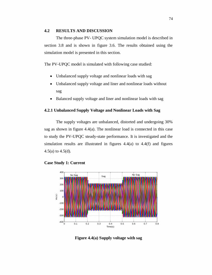
4.2.1 Unbalanced Supply Voltage and Nonlinear Loads with Sag
The supply voltages are unbalanced, distorted and undergoing 30%
sag as shown in figure 4.4(a). The nonlinear load is connected in this case
to study the PV-UPQC steady-state performance. It is investigated and the
simulation results are illustrated in figures 4.4(a) to 4.4(f) and figures
4.5(a) to 4.5(d).
Case Study 1: Current
Figure 4.4(a) Supply voltage with sag
0 0.1 0.2 0.3 0.4 0.5 0.6 0.7 0.8-400
-300
-200
-100
0
100
200
300
400
Time(s)
SagNo Sag No Sag

75
Figure 4.4(b) Load current
Figure 4.4(c) Load current (THD=14.3%)
Figure 4.4 (d) Current injected by shunt active filter

76
Figure 4.4 (e) Supply current (THD=1.15%)
Figure 4.4(f) Phase A –Supply, Load and Injected currents
Figure 4.4 (c) shows the load currents, which are highly distorted.
The THD is 14.3%, whereas according to IEEE Standard 519-1992 they
should not exceed 5% in our case. The effects of the injection of
compensating currents are shown in figure 4.4 (d). Figure 4.4(e) shows the
harmonics minimization sinusoidal wave (THD=1.15%), which fulfills the
5% stipulated by the IEEE standard. From figure 4.5 (e), the supply current

77
is in-phase with the load voltage, which is due to the in-phase series
voltage injection. The injection is in-phase with the fundamental of the
supply voltage. Thus, no reactive power is drawn from the supply. In figure
4.4 (f), the supply current, load current and injected current of are plotted
together. If the injected current wave is subtracted from the load current
wave, the result will be the supply current wave.
Case Study 1: voltage
Figure 4.5 (a) Supply voltages (THD=7.7%)
Figure 4.5 (b) Voltages injected by series active filter

78
Figure 4.5 (c) Load voltage (THD=0.7%)
Figure 4.5 (d) DC link voltages
Figure 4.5 (e) Phase A load voltage and supply current

79
Figure 4.5(f) Phase A supply voltages, injected and load voltages
From figure 4.5 (a), the supply voltages are unbalanced, distorted
(THD=7.7%) and undergoing a sag. The series compensator injects
voltages as shown in figure 4.5 (b). Due to this series compensation, the
voltages on the load side are balanced sinusoidal. Figure 4.5(c) shows
THD of 0.7%, which is much below the 5% limit stipulated by the IEEE
Standard. It can be seen from figure 4.5 (c) that the load voltages are kept
at the nominal level of 325 volts. The load and injected voltages for phase
A are plotted together. The sum of the injected voltage and the supply
voltage is the load voltage.
In figure 4.5 (d), the concept of dc link voltage has been illustrated.
The shunt compensator is connected at 0.02s which causes a drop in dc link
voltage. After the sag from 0.02 s to 0.5s, the dc link voltage is restored.
From figure 4.5 (d), it is observed that the average dc link voltage is kept
constant at 400 V.

80
Case Study 2
4.2.2 Linear and nonlinear loads without sag
The supply voltages, as shown in figure 4.6(a), are unbalanced and
distorted (the 5th harmonic is present) but there is no sag this time. The
nonlinear load is permanently connected and the linear load is connected at
0.2s and disconnected at 0.5s. In this case study, the PV-UPQC dynamic
performance at load change is investigated and the simulation results are
illustrated through the figures 4.6 to 4.10.
Case Study 2: load currents
Figure 4.6 (a) Load current dynamics
81
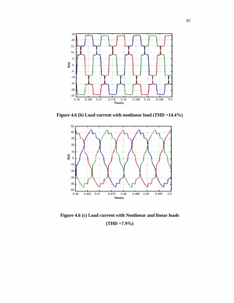
Figure 4.6 (b) Load current with nonlinear load (THD =14.4%)
Figure 4.6 (c) Load current with Nonlinear and linear loads
(THD =7.9%)

82
Figure 4.6 (d) Load current with Nonlinear load (THD = 14.4%)
The simulated duration is composed of three sub-intervals:
0 s to 0.2 s, only with the nonlinear load connected to the system
0.2 s to 0.5 s, with both the linear and nonlinear loads connected to
the system
0.5 s to 0.8 s, only with the nonlinear load is connected to the
system
For clarity, the load current waveforms, shown in figure 4.6(a), for
each of these three subintervals is zoomed in figures 4.6 (b) to 4.6 (d). The
injected and supply currents are shown in figures 4.7 and 4.8. The load
current changes are reflected in both injected and supply currents. A
change in the load causes the system to go through a transient period after
which the supply currents become balanced sinusoids, as shown in figures
4.8(b) to 4.8(d), in phase with the load voltage as shown in figure 4.10.
Thus, the PV-UPQC adjusts the injected current according to the load
condition, ensuring that, in steady-state, the supply currents are always
balanced sinusoids and no reactive power is drawn from the supply.

83
Figure 4.7 (a) Injected current dynamics
Figure 4.7 (b) Injected current with nonlinear load
0 0.1 0.2 0.3 0.4 0.5 0.6 0.7 0.8-25
-20
-15
-10
-5
0
5
10
15
20
25
Time(s)
Nonlinearload
Nonlinear load
Linear and Nonlinear loads

84
Figure 4.7(c) Injected current with linear and nonlinear loads
Figure4.7 (d) Injected current for nonlinear load
Figure 4.8(a) Supply current with dynamics

85
Figure 4.8 (b) Source current with nonlinear load (THD =2.4%)
Figure 4.8 (c) Source current with nonlinear and linear loads
(THD =1.3%)
Figure 4.8(d) Source current with nonlinear load (THD=2.4%)

86
During the entire simulation period (from 0s to 0.8 s), the supply
voltages are unbalanced and distorted (THD=5.05%), as shown in figure
4.9 (a). The injected voltage by the series compensator is shown in figure
4.9 (b). Due to this series compensation, the voltages on the load side are
balanced sinusoidal waveforms, as shown in figure 4.9(c), with THD 1%,
which is much lower than the 5% limit recommended by IEEE Standard
519-1992. From figure 4.9(c), it can be seen that the load voltages are kept
at the nominal level (325 V).
Figure 4.9 (a) Supply voltage (THD = 5.05%)
Figure 4.9 (b) Inverter injected voltage

87
Figure 4.9 (c) Load voltage (THD=1%)
Figure 4.9 (d) DC link Voltage
The DC link voltage dynamics is shown in figure 4.6(d).The load
current increases at 0.2s and decreases at 0.5s. This is due to the connection
or disconnection of the linear load. Since it takes a finite time interval to
calculate the new reference current, the shunt compensator cannot
immediately respond to the load change. Some settling time is required to
stabilize the controlled parameter around its reference. During transient
periods, the DC link capacitor is supplying active power in order to ensure
the power balance.

88
Figure 4.10 (a) Load voltage and load current with nonlinear load
Figure 4.10(b) Load voltage and load current with nonlinear and
linear loads
Due to this transient supply of active power, the dc link voltage
decreases during the sag at the time interval of 0.2s – 0.4s and the swell in
the voltage occurs during the interval 0.5s – 0.7s. After clearing the

89
interruptions, as illustrated through the figure 4.6 (d), the dc link voltage is
restored back to its reference value (400 V).
The shunt compensator is controlled in such a way that the supply
current is in-phase with the fundamental of the supply voltage, which
means that no reactive power is drawn from the supply. The fundamental
of the series injected voltage is in-phase with the supply current, as shown
in figure 4.10.
Case study 3
4. 2.3 Balanced linear and nonlinear loads with sag
During the time interval from 0s to 0.8 s, both the linear and
nonlinear loads are connected with 30% of supply voltage sag, which is
generated at 0.2 s and cleared at 0.5 s. During the same time, the supply
voltage becomes balanced and distorted (the 5th harmonic is present). The
supply voltages are as shown in figure 4.11(a) and figure 4.11 (e) Supply
current during the sag with fuzzy logic control.
In this case study, the dynamic performance of the PV-UPQC
system, at the occurrence or clearance of the supply voltage sag, is
investigated and the simulation results are illustrated through figures 4.11
to 4.15.
The supply current is increased considerably during the sag, as
shown in figure 4.12. During the sag, the load should draw the same
amount of power from the supply as it does in the normal condition
(nominal power). Since the supply voltage is decreased during the sag, the
supply current should be accordingly increased in order to provide the
same nominal power to the load.

90
Figure 4.11 (a) Supply current with dynamics
Figure 4.11 (b) Supply current before sag (THD=3.8%)
Figure 4.11(c) Supply current during the sag (THD=1.1%)

91
Figure 4.11 (d) Supply current after the clearance sag (THD
=3.8%)
Figure 4.11 (e) Supply current during the sag with fuzzy logic
control (THD=1.2%)
The supply voltage dynamics are shown in figure 4.12(a). During
the sag condition from 0.2 s to 0.5s, the supply voltages undergo 60% sag.
They are unbalanced and distorted with THD of 7.7%, as shown in figure
4.12 (c). During the other two sub-intervals from 0s to 0.2s and from 0.5s
to 0.8s, the supply voltages are balanced sinusoidal waveforms at nominal
level (325V), as shown in the figures 4.12 and 4.13.

92
Figure 4.12 (a) Supply voltage with dynamics
Figure 4.12 (b) Supply voltage before sag (THD=0.55%)
0 0.1 0.2 0.3 0.4 0.5 0.6 0.7 0.8-400
-300
-200
-100
0
100
200
300
400
Time(s)
SagNo Sag No Sag

93
Figure 4.12 (c) Supply voltage during sag (THD=7.7%)
Figure 4.12 (d) Load voltage after the clearance of sag (THD=0.55%)
Figure 4.13 (a) Voltages injected during sag

94
Figure 4.13(b) DC link voltage during sag
Figure 4.14 (a) Load voltage with dynamics
Figure 4.14 (b) Load voltage before sag (THD=1.4%)
0 0.1 0.2 0.3 0.4 0.5 0.6 0.7 0.8-400
-300
-200
-100
0
100
200
300
400
Time(s)
No sag No sag Sag

95
Figure 4.14 (c) Load voltage during sag (THD=0.75%)
Figure 4.14 (d) Load voltage sag with ANN controller (THD=1.2%)
During the supply voltage sag, the series compensator injects
voltages, as shown in figure 4.14(a). Due to this series compensation, the
voltages on the load side are balanced sinusoidal waveforms with THD of
0.75%, which is much lower than the 5% limit recommended by IEEE
Standard 519-1992, as shown in figure 4.14(c) and figure 4.14 (d) shows
the load voltage sag with ANN controller. Figure 4.15 shows that the load
voltages are kept at the nominal voltage throughout the simulation time
interval.
96
The DC link voltage dynamics are shown in figure 4.13 (b). Due to
the occurrence of the supply voltage sag at 0.2 s, the supply current is
increased. With the clearance of sag at 0.5s, the supply current decreased.
Since it takes a finite time interval to calculate the new reference current,
the shunt compensator cannot immediately respond to this supply current
change. Some settling time is required to stabilize the controlled parameter
around its reference.
Consequently, after the occurrence or clearance of the sag instants
(0.2s and 0.5s), there exist some transient periods during which the DC link
capacitor is supplying active power in order to ensure the balanced power.
Due to this transient supply of active power, the DC link voltage is
undergoing sag during the time interval 0.2 s – 0.4 s and a swell during the
interval 0.5 s – 0.7 s. From figure 4.14 (d), it can be observed that after
clearing the transients, the DC link voltage is restored back to its reference
value (400 V).
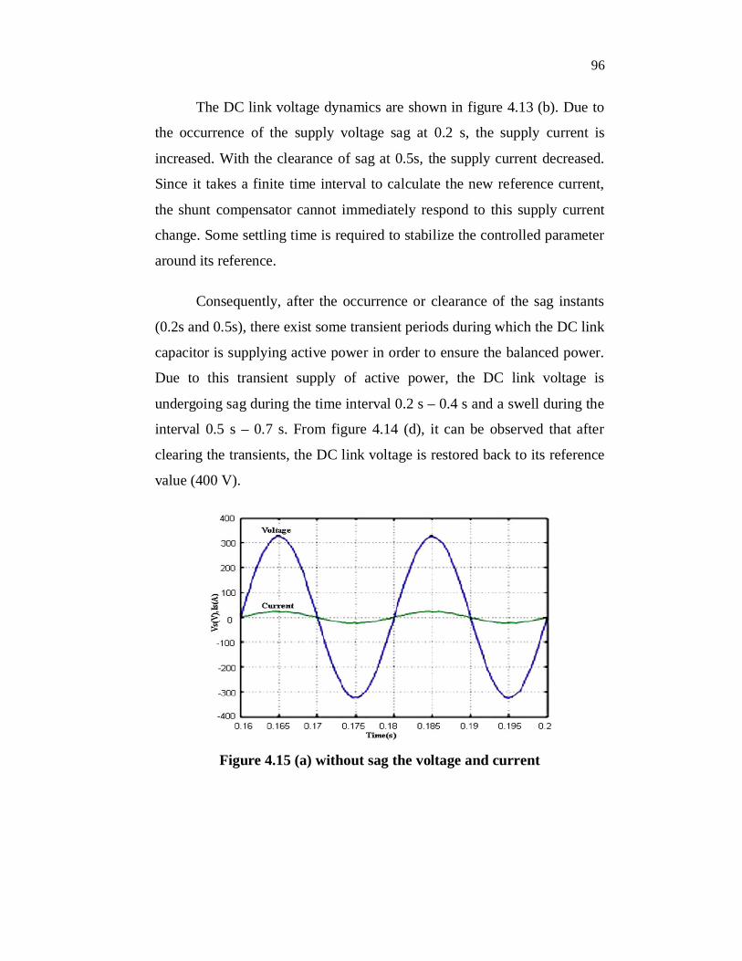
Figure 4.15 (a) without sag the voltage and current

97
Figure 4.15 (b) during sag the voltage and current
Figure 4.15(c) after clearance of the sag voltage and current
Due to unity power factor compensation throughout the entire
simulated period, the supply current is in phase with the fundamental of the
supply voltage, as shown in figure 4.15, which implies that no reactive
power is drawn from the supply.
A complete summary of the results with and without the proposed
system is given in table 4.1 and in figures 4.16 to 4.21.

98
Table 4.1 Comparative percentage THD voltage and current with and
without PV-UPQC system.
Casestudy No’s
Events
Without PV-UPQC
With PV-UPQC
Current %THD
Voltage %THD
Current %THD
Voltage %THD
1Unbalanced supply voltage nonlinear loads with sag
14.3 7.7 1.15 0.7
2
Unbalanced supply voltage linear and nonlinear loads without sag
14.4 5.05 1.3 1
3
Balanced supply voltage linear and nonlinear loads with sag
14.18 7.7 1.1 0.55

99
Figure 4.16 Percentage THD with and without PV-UPQC for
nonlinear loads with sag and unbalanced supply voltage
Figure 4.17 Percentage THD with and without PV-UPQC for
unbalanced supply voltage linear without sag and nonlinear loads

100
Figure 4.18 Percentage THD with and without PV-UPQC for balanced
supply voltage with sag and linear and nonlinear loads
Figure 4.19 Percentage THD with and without PV-UPQC for
unbalanced supply voltage with sag and nonlinear loads

101
Figure 4.20 Percentage THD with and without PV-UPQC for
unbalanced supply voltage without sag with liner and nonlinear loads
Figure 4.21 Percentage THD with and without PV-UPQC for balanced
supply voltage with sag and nonlinear loads

102
Table 4.2 THD values of load current with fuzzy logic control Rama
Rao et al (2010) and proposed PI with hysteresis control
THD load current
without controller
Fuzzy logic control
THD load currents
Proposed PI with
hysteresis control THD
load currents
14.3% 1.2% 1.1%
Figure 4.22 Percentage THD for fuzzy logic control and proposed
hysteresis control

103
Table 4.3 THD value of load voltage Artificial Neural Networks
(ANN) Jeno Paul et al (2011) and proposed PI with hysteresis control
THD for load voltage without
controller
ANN control THD load voltage
PI with Hysteresis control THD load voltage
7.7% 1.2% 0.55%
Figure 4.23 Percentage THD for ANN control and proposed hysteresis
control
The performance evaluation of PV-UPQC system associated with
linear and nonlinear loads with sag using hysteresis control, in terms of the
THD of the load current, is given in table 4.2. Comparing with the results
of THD of 1.2% in the load current obtained using an ANN control by
Jeno Paul et al (2011), the proposed hysteresis control has achieved a lower
THD of 1.1%, which is shown in figure 4.22.
Comparing with the results of THD of 1.2% in the load voltage
obtained using a fuzzy logic control by Rama Rao et al (2010), the
proposed hysteresis control has achieved a lower THD of 0.55% as shown
in table 4.3 and figure 4.23. The analysis shows that the proposed

104
approach is more efficient with respect to ANN and fuzzy logic control
strategies.
On the basis of the research work presented in this chapter, a paper
entitled ‘Photovoltaic based improved power quality using unified power
quality conditioner’ has been published in the International Journal of
Electrical Engineering Vol.4, No.2, pp.227-242, July 2011.
On the basis of the research work presented in this chapter, a paper
entitled ‘Power Quality Improvement using Photovoltaic Compensation
Techniques’ has been published in the International Journal of Power
Engineering Vol.2, No.1, pp. 33-46, June 2010.
4.3 CONCLUSION
In this chapter, three significant case studies of an unbalanced
system with linear and nonlinear loads are presented. The first case is
supply voltage sag with nonlinear loads. The second case is linear and
nonlinear loads without sag. The third case is linear and nonlinear loads
with sag. The simulation results shows that the linear and nonlinear loads
are connected the voltage becomes unacceptably distorted due to the
switching frequencies in the supply current.
For comparative analysis of the proposed PI with hysteresis control,
the fuzzy logic and ANN control strategies of other researchers have been
considered. Among various control techniques, the proposed hysteresis
current control is the most preferable technique for shunt compensation.
The hysteresis control method has simpler implementation, enhanced
system stability and fast response. The proposed approach ensures that the
unwanted harmonics are reduced compared to the other control strategies.