Chapter 7. Electrons in a solid I. One electron approximation 1. Total (non-relativistic) Hamiltonian of a lattice:

2. Large difference between electron and nuclear masses ⇒ Nuclei kinetic energy can be neglected. 3. If the nuclei have a fixed configuration, the nucleus-nucleus is a constant term and it can be disregard if we are considering just the electronic states. 4. Hence the many-body Hamiltonian for a system of N interacting electrons in the presence of nuclei can be written in the form

The goal is to find the solution of the Eigenvalue problem HeΨ(r1σ1, r2σ2,…. ,rNσN)= EΨ(r1σ1, r2σ2,…. ,rNσN) 5, Hartree approximation 1: The total wave function Ψ is a product of orthonormalized one-electron wave functions ψ:

Ψ(r1σ1, r2σ2,…. ,rNσN)= ψ1(r1σ1)ψ2(r2σ2)… ψN(rNσN) The subscript i in riσi indexes the electrons. The subscript i in ψi indexes the wave function. ψ is the product of two parts – spatial ϕ(r) and spin χ(σ) so that ψ( rσ)= ϕ(r)χ(σ). The problem is now to determine ψ(rσ). 6. The electron charge density is given by

The summation is over all electrons. 7. Hartree approximation 2:

|Rr|eZ )r(V

|RR|eZZ

21

|rr|e

21 )r(V

M2p

m2p H

J

2I

Inucl

ninteractio nucleus-nucleus

JI

2jI

JI

ninteractioelectron -electron

ji

2

ji

ninteractio nucleus-electron

inucli

KE Nuclei

I

2I

I

KE electrons'

2i

iTot

vvv

44 344 21

vv

4434421

vv43421

v

43421

v

43421

v

−−=

−+

−+++=

∑

∑∑∑∑∑≠≠

ij

2

jiinucl

2i

i

ninteractioelectron -electron

ji

2

ji

ninteractio nucleus-electron

inucli

KE electrons'

2i

ie

re

21 )r(V

m2p

|rr|

e21 )r(V

m2p

H

vv

v

44 344 21

vv43421

v

43421

v

∑∑

∑∑∑

≠

≠

++=

−++=

)r()r(*(-e) )r( iii

vvv ϕϕ=ρ ∑

The Coulomb potential experienced by an election due to other electrons is approximated by the Hartree potential Vcoul, which is actually the potential due to all electrons. It is further assumed that all electrons experience the same potential. In this way, the multi-electrons problem is reduced to one electron problem.

From these we have the Hartree equation:

8. The solution is a set of wave function ψ1,ψ2… ψNdetermined by self-consistency:

'rd)'r(|'rr|

1)'r(* 'rd|'rr|

)'r( )r(V 3

ii

j

3

jCoul

vvvv

vvvv

vv

−ϕ=

−ρ

= ∫∑∫∑

iiiCoulinucl

2

)r(V )r(Vm2

pψε=ψ⎥

⎦

⎤⎢⎣

⎡++ vv

v

Guess a set of wave functions ψ1,ψ2… ψN

Calculate Hartree Potential Vcoul with the wave functions.

Solve Hartree equation with Vcoul just calculated and get a new set of wave functions.

Is the difference between the new and the old sets of wave functions small enough?

The set of wave functions is the solution. Can continue to calculate εi.

9. Problem of the Hartree approximation: the wave functions do not take into the fact that electrons are Fermion and hence the wave function ψ(rσ) should be anti-symmetric (i.e. Pauli exclusion principle). II. Hartree-Fock equation 1. If ψ1(r1σ1)ψ2(r2σ2)… ψN(rNσN) is a solution of HeΨ= EΨ, then so is any permutation like ψ1(rNσN)ψ2(r2σ2)… ψN(r1σ1) and any linear combination of these permutations. 2. Electron is a Fermion, exchanging any two electrons will change sign of the wave function, i.e. Ψ(r1σ1, r2σ2,…. ,rNσN) = - Ψ(rNσN, r2σ2,…. ,r1σ1) and so on. 3. Furthermore, no two electrons can occupy the same state. For example, ψ1(r1σ1)ψ2(r2σ2)… ψ1(rNσN) =0 4. The Slater determinant constructed from ψ1(rNσN), ψ2(r2σ2), … ψN(r1σ1) processes all of the above properties: 5. The Hamiltonian matrix element for the total wave function can be calculated for the Slater determinant:

hand.)short (in detN!1

)r()r()r(

)r()r()r()r()r()r(

N!1 )r,r,r(

N21

NNN22N11N

NN2222112

NN1221111

NN2211

ψψψ

σψσψσψ

σψσψσψσψσψσψ

σσσ

L

vL

vvLLLL

vL

vv

vL

vv

vL

vv

=

=Ψ

)r()r(Vm2

p )r(

N!)r(N!1)r(V

m2p )r(

N!1

detN!1)r(V

m2p det

N!1

)r,r,r()r(Vm2

p )r,r,r(

iiiinucl

2i

iiii

iiiinucl

2i

iiii

N21inucl

2i

nspermutatio N!

N21i

NN2211inucl

2i

iNN2211

σψσψ

σψσψ

ψψψψψψ

σσσσσσ

vvv

v

vvv

v

Lv

v

43421L

vL

vvvv

vL

vv

+=

×+=

+=

Ψ+Ψ

∑

∑

∑

∑

The electron-electron repulsive energy on the antisymmetric wave function is always lower than the repulsive energy on the “simple” wave function used in the Hartree equation. 6. Hartree-Fock equation can be obtained by variational principle in minimizing <Ψ|He|Ψ> under the constraint that <ψi|ψj>=δij. Apply Lagrange multipliers εij: Define Operators:

><−

⎥⎥⎦

⎤

⎢⎢⎣

⎡−+

+=

∑

∑

)r(|)r(

)r()r(re )r()r()r()r(

re )r()r(

21

)r()r(Vm2

p )r( E

jjjiiiij

jjiiijij

2

jjjiiijjjiiiij

2

jjjiiij,i

iiiinucl

2i

iiii

σψσψε

σψσψσψσψσψσψσψσψ

σψσψ

vv

vvv

vvvvv

vv

vvv

v

44444444 344444444 21

vvv

vvvvv

vv

vvv

vv

vvv

vv

Lv43421L

vL

vvv

vL

vv

" Exchange"

jjiiijij

2

jjjiiiji

jjjiiiij

2

jjjiiiji

jjiiijij

2

jijjjiii

jjjiiiij

2

jijjjiii

N21ij

2

jinspermutatio N!

N21

NN2211ij

2

jiNN2211

)r()r(re )r()r(

21)r()r(

re )r()r(

21

N!)r()r(N!1

re

21 )r()r(

N!1-

)r()r(N!1

re

21 )r()r(

N!1

detN!1

re

21 det

N!1

)r,r,r(re

21 )r,r,r(

σψσψσψσψσψσψσψσψ

σψσψσψσψ

σψσψσψσψ

ψψψψψψ

σσσσσσ

∑∑

∑

∑

∑

∑

≠≠

≠

≠

≠

≠

−=

×⎪⎭

⎪⎬⎫

⎪⎩

⎪⎨⎧

=

=

ΨΨ

Define operators:

Above equation reduces to a single electron equation:

Diagonalize ε so that εij = εiδij, we have the Hartree-Fock equation:

)r(

)r()r(re )r()r()r(

re )r()r()r(V

m2p

)r(|)r(

)r()r(re )r()r()r()r(

re )r()r(

)r()r(Vm2

p )r(

0E :0 | s variationand |ariation arbitray vConsider

jjjij

jjiiijij

2

jjjiiijjjij

2

jjjj

iiiinucl

2i

jjjiiiij

jjiiijij

2

jjjiiijjjiiiij

2

jjjiiij,i

iiiinucl

2i

iiii

ii

σψε

σψσψσψσψσψσψσψ

σψσδψε

σψσψσψσδψσψσψσψσδψ

σψσδψ

δδψδψ

v

vvv

vvvv

vvvv

vv

vvv

vvvvv

vv

vvv

v

=

⎥⎥⎦

⎤

⎢⎢⎣

⎡−+⎟

⎟⎠

⎞⎜⎜⎝

⎛+⇒

><=

⎥⎥⎦

⎤

⎢⎢⎣

⎡−+

+⇒

=≡><

∑

∑

∑

j3

jjij

2

jjjjj

j3

jjijj

2

jjjj

iijjjiij

2

jjjj

jjiiijij

2

jjjj

iexch

ij3

jjjj

2

jj*

jj

jjjij

2

jjjj

iCoul

rd)r(|r-r|

e)r()r(-

rd)r()r(|r-r|

e)r(-

))r()r(re )r(( )r()r(

re )r( )r()r(V

)r(rd)r(|r-r|

e )r(

)r(re )r()r()r(V

vvvv

vv

vvvvv

v

vvv

vvvv

vvv

vvvvv

v

vv

vvv

σψσψσψ

σψσψσψ

σψσψσψσψσψσψψ

ψσψσψ

σψσψψ

∫∑

∫∑

∑∑

∫∑

∑

=

=

−=−=

⎥⎥⎦

⎤

⎢⎢⎣

⎡=

=

)r()r()r(V)r(V)r(Vm2

piiiijiiiiexchiCoulinucl

2i σψεσψ vvvvvv

=⎟⎟⎠

⎞⎜⎜⎝

⎛−++

)r()r()r(V)r(V)r(Vm2

piiiiiiiiexchiCoulinucl

2i σψεσψ vvvvvv

=⎟⎟⎠

⎞⎜⎜⎝

⎛−++

III. Free electron 1. Screening of nuclei potential by inner electrons ⇒ Vnucl = 0. 2. Low electron density, screening by free electrons (Thomas-Fermi screening) and the rareness of electron-electron scattering ⇒ VCoul = Vexch =0. 3. For free electrons: 4. For free electrons: Determination of Fermi energy EF: Dispersion relation: Density of state: Temperature effect:

rkiiiiiiiiiii

2i e)r( )r()r(m2

p vvvvvv

⋅=⇒=⎟⎟⎠

⎞⎜⎜⎝

⎛σψσψεσψ

kx

ky

kz

kF

Fermi sphere

n 3k N

V8

k34

2 3

3F

3

3F

=⇒=×ππ

π

m2k E

22h=

dEdkkV D(E) D(E)dE

V8

dkk42 223

2

ππ

π=⇒=×

Note that µ(0)=EF. IV. Central equation 1. A crystal possesses lattice symmetry, and hence there must be some potential for the electron with the same periodicity, no matter how small is the potential (in case of nearly free electron). The one electron Schroedinger equation:

where V is the periodic potential. 2. Bloch’s theorem. The solution of the one electron Schroedinger equation is always in the form:

where uk(r) is a periodic function that has the same periodicity as the lattice: uk(r+R) = uk(r) Note that ψk(r) does not have the same periodicity as the lattice because ψk(r)≠ ψk(r+R). Instead,

This equation is considered as Bloch’s theorem also (in another form). 3. Because of the periodicity, eiK⋅r forms a complete orthogonal set of functions. Any function with the same periodicity as the lattice can be expressed as a linear combination of eiK⋅r:

4. The one electron Schroedinger equation can be reduced to the Central equation:

Central equation relates C(k) and C(k+K) for all reciprocal vectors K. There is one central equation for each allowed value of k. The dispersion relation of electron can be obtained by requiring the determinant of this set of linear equations to be zero (for a non-trivial solution). 5. ψk(r) in terms of C(k):

1e

1 f(E)Tk(T)-E

B +

= µ

ψ=ψ+ψ∇− E V m2

22h

rkikk e)r(u )r(

vv

vvvv ⋅=ψ

0 )K k(CV )k(CEm2k K

K

22

=−+⎟⎟⎠

⎞⎜⎜⎝

⎛− ∑

vvvhv

v

rd)erV(V1V eV )rV( 3rKi-

CellK

rKiK

K

vvv v

v

v

vv

⋅⋅ ∫∑ =⇒=

)r(ee)r(uee)r(u )Rr( kRkirki

kRki)Rr(ki

kkvvvvv

v

vvvv

v

vvvvv

vv ψ===+ψ ⋅⋅⋅+⋅

rkirKi

Kk e e)Kk(C )r(

vvvv

vv

vvv ⋅−⋅−−=ψ ∑

Compare with Bloch’s theorem, we know that

6. Now look at the Central equation, there is one equation for each value of k (-∞<k<∞). However, only k, k+K, k+K’, k+K”,….are related together within the same group of equation. For the sake of discussion, let us assume there are N real space lattice points and M reciprocal space lattice points (N, M →∞). There is a total number of N×M central equations for the N×M unknown C(k). However, since only only k, k+K, k+K’, k+K”,… (M of them) will appear in the same central equation (M of them), hence the N×M central linear equation system is actually block diagonalized into M×M blocks and there are N of these blocks. 7. This block diagonization allows us (and more reasonable) to present the dispersion relationship of single electron in the reduced zone scheme: instead of using the N×M k (-∞<k<∞) values to index the solution (extended zone scheme), we can use k (limited to the first Brillouin zone, N of them) and K (M of them) to index the solution (reduced zone scheme). If is more often to use n (=1,2, ….M) instead of K in labeling the solution.

)r(ue)Kk(Cee)Kk(Ce)Kk(C )Rr(u

:lattice theasy periodicit same thehasit and )r(u e)Kk(C

krKi

K

RKirKi

K

)Rr(Ki

Kk

krKi

Kvvvvvvvvv

vvv

vvv

v

vvvv

v

vvv

vv

vvv

v

=−=−=−=+

=−

⋅−⋅−⋅−+⋅−

⋅−

∑∑∑

∑

C

CC

C

CC

C

CC

C

CC

C

CC

C

CC

MN

1N

N

M2

12

2

M1

11

1

MN

1N

N

M2

12

2

M1

11

1

Kk

Kk

k

Kk

Kk

k

Kk

Kk

k

Kk

Kk

k

Kk

Kk

k

Kk

Kk

k

⎟⎟⎟⎟⎟⎟⎟⎟⎟⎟⎟⎟⎟⎟⎟⎟⎟⎟⎟⎟⎟⎟⎟⎟

⎠

⎞

⎜⎜⎜⎜⎜⎜⎜⎜⎜⎜⎜⎜⎜⎜⎜⎜⎜⎜⎜⎜⎜⎜⎜⎜

⎝

⎛

⎟⎟⎟⎟⎟⎟⎟⎟⎟⎟⎟⎟⎟⎟⎟⎟⎟⎟⎟⎟⎟⎟⎟

⎠

⎞

⎜⎜⎜⎜⎜⎜⎜⎜⎜⎜⎜⎜⎜⎜⎜⎜⎜⎜⎜⎜⎜⎜⎜

⎝

⎛

=

⎟⎟⎟⎟⎟⎟⎟⎟⎟⎟⎟⎟⎟⎟⎟⎟⎟⎟⎟⎟⎟⎟⎟⎟

⎠

⎞

⎜⎜⎜⎜⎜⎜⎜⎜⎜⎜⎜⎜⎜⎜⎜⎜⎜⎜⎜⎜⎜⎜⎜⎜

⎝

⎛

+

+

+

+

+

+

+

+

+

+

+

+

vr

vr

r

vr

vr

r

vr

vr

r

vr

vr

r

vr

vr

r

vr

vr

r

M

M

M

M

M

M

M

M

M

M

M

M

M

M M×M

M×M

M×M

M×M

0

0

M×N

M×N

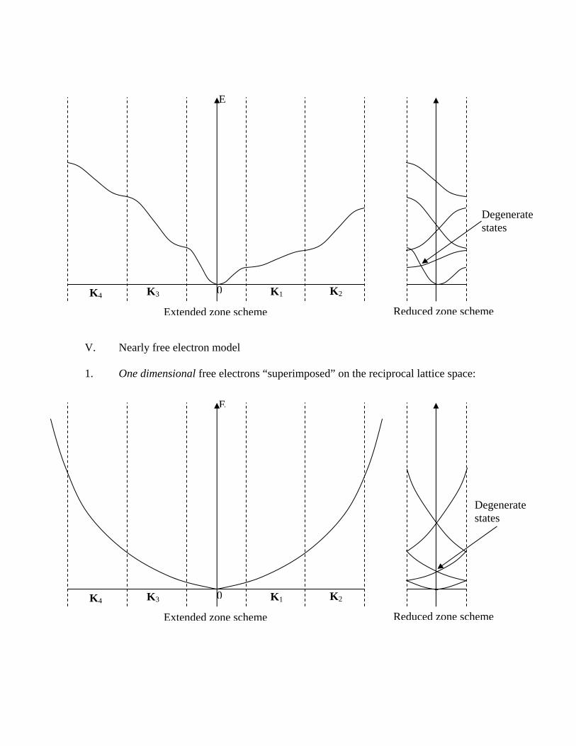
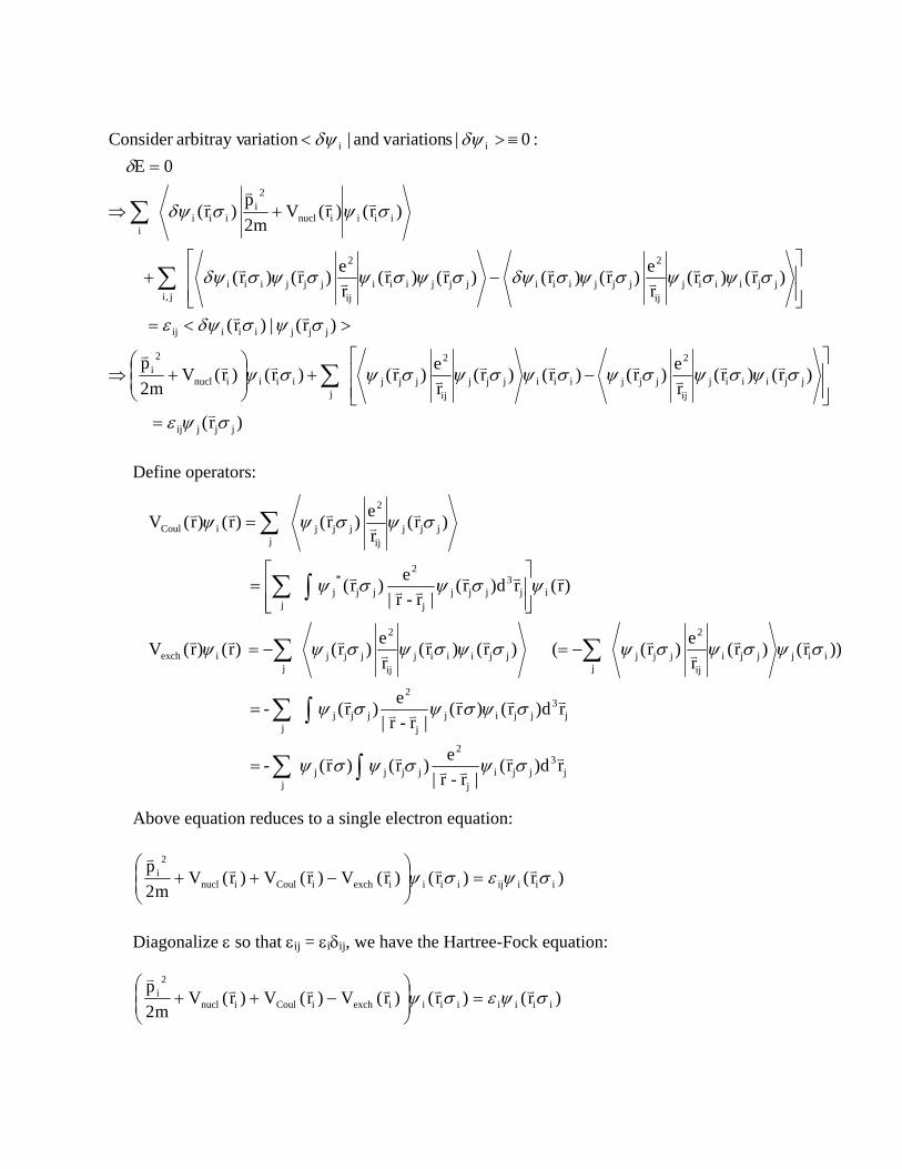
V. Nearly free electron model 1. One dimensional free electrons “superimposed” on the reciprocal lattice space:

0 K1 K2 K3 K4

E

Degenerate states

Extended zone scheme Reduced zone scheme

Degenerate states

Reduced zone scheme

0 K1 K2 K3 K4

E

Extended zone scheme

2. If there is no potential, the electron will be perfectly free, but there will be no periodicity either. Hence, for the existence of lattice periodicity, there must be some potential, no matter how weak, possessing the same periodicity as the lattice. 3. If the potential is very weak, the dispersion relationship for the single electron should be very similar to that of free electron and the wave function of the electron should look like the plane wave eik⋅r. 4. In reduced zone scheme, degenerate states will occur (see figures above). Bragg’s scattering will remove the degeneracy and create band gap. For this reason, it is not practical to label the band with reciprocal vector K. 5. Sketching Fermi surfaces (i) Construct enough Brillouin zone to contain the Fermi sphere (i.e. construction in extended zone scheme). (ii) Draw the Fermi sphere to hold all electrons (iii) Rearrange different zone region into one piece (reduced zone scheme) ⇒ possible to have several Fermi surfaces. (iv) “Round off” corners. By crystal symmetry, Fermi surface always perpendicular to zone boundary.

K

K’ 2|VKK’|

N 2

V8

k34

spin3

3F

=×π

π

VI. Tight binding model 1. Also known as Linear Combination of Atomic Orbital (LACO). 2. This model starts from isolated atoms and atoms can “share” electrons by overlap of atomic orbital. Model works fine for the d-bands of transition metals and also valance bands of insulators. 3. Atomic orbital: s orbital (l=0 with mz=0), can hold two electrons. Group notation: a1g (a=non-degenerate, g= inversion symmetry) p orbital (l=1 with mz=0, ±1 ), can hold 6 electrons. \ Group notation: t1u (t=triple degeneracies) d orbital (l=2 with mz=0, ±1, ±2), can hold 10 electrons. Group notation: t2g (t=triple degeneracies)

px

dxy

py pz

dxz

dxz

Group notation: eg (e=double degeneracies) 4. Mixint of different orbital ⇒ Hybridization. E.g. s-d hybridization. 5. ρ

γα

ϕρϕϕϕvv

v

444 3444 21

vvvv

444 3444 21

vvv ⋅

−

∑∫∫ += k-i

nn

3*

-

3*k er)dr()H-r( r)dr()Hr( E

where nn=nearest neighbors and ρ is the vector pointing to the nearest neighbor vector. For example, there are six nearest neighbors for simple cubic.

a)k cos ak cos ak (cos2- - ]eeeee[e - - E

a).(0,0, a,0),(0, a,0,0),(

zyx

aikaik-aikaik-aikaik-k

zzyyxx

++=

+++++=∴

±±±=

γαγα

ρv

6. Band width: Narrow band with small bandwidth ⇔ Higher effective mass m* ⇔ Lower mobility. A material with a very narrow bandwidth is an insulator (Mott insulator). A metal-insulator (Mott) transition by adjusting the bandwidth is called Mott transition. One way to achieve Mott transition is to increase the atomic separation a and reduce the overlap of atomic orbitals. VII. Semiclassical model

dz2 dx

2- y2

E

k

Bandwidth W

1. A single particle in k-space (occupying a unique state) will produce a wave u(r)eik⋅r in real space. Similarly, a single particle in real space is a wave in k-space. In semi-classical model, a compromise is made so that the single electron wave function is “Gaussian” like in both reap space and k-space: In this way the electron is “particle like” in both real space and k-space. Physical quantities like position and velocity can be measured by the mean of the Gaussian functions. 2. Equations of motion: For example, one-dimensional free electrons case, In the presence of electric and magnetic field, 3. Effective mass of an electron at state k: The effective mass is actually a tensor [m*(k)] with its inverse defined as

ψ

r

ψ

k

k p F

E 1v k

&vh&vv

h

vv

==

∇=

vmp

mk

dkdEE

m2k E

2

k

22

hhhh

v ====∇⇒=

)BvEe(- k )BvE-e( F vvv&vh

vvvv×+=⇒×+=

m1

m1

m2k

k1

kk)kE(1

electron, free D-1For :Example

kk)kE(1 ])k(*m[

2

2

22

2

2

2ji

2

2

ji

2

2ij1-

==⎟⎟⎠

⎞⎜⎜⎝

⎛∂∂

=∂∂

∂

∂∂∂

±=

h

h

h

h

v

h

v

h

v

Notes: (i) There are two signs for the mass tensor. Positive sign is for electron and negative sign is for hole. (ii) Near the extremums of the energy band, m-1 is a measure of the parabolic curvature. 4. 5. Semiclassical model does not allow interband transition. i.e., n remains constant for a particular electron. 6. The equations of motion apply only to an electron in the time between two collisions. Immediately after a collision, the electron will be scattered in random direction (Drude model) and the equations of motion will be followed again until the next collision. 7. Effect of external force: If there is no collision (i.e. no resistance)

vM F ed,diagonaliz is tensor mass theIf

vM F k p F

:space realin have weTherefore, k vM

kM v

it

k kk

)kE( 1v

x)y,x,(i i k

)kE( 1 v E 1v

ijij

jiji

jij1-

i

i

ii

2

ii

iik

&vv

&&vh&vv

&h&

&h&

v

h&

v

hh

vv

=

=⇒==

=⇒

=⇒

∂∂

∂∂∂

=⇒

=∂∂

=⇒∇=

∑

k

E

k

E

Larger m-1 ⇒ smaller m Smaller m-1 ⇒ larger m ∴ narrow band ⇒ larger m

The Fermi sphere will translate across the d-space: Un-free electron No interband transition ⇒ the Fermi surface will “oscillate” and remain in the first Brillouin zone. Over time, it will “disappear” at the zone boundary but reappear immediately at the opposite zone boundary as shown in the above figure. If there is collision (as in all real cases): The Fermi surface will remain stationary in k-space. On average, the sphere has only a time of τ (relaxation time) to translate across the k-space.

Free electronF

ky

kx ∆k

constant is force if tF

dt F k F k k p F

h

vh

vv

h

v&v&vh&v

v

=

=∆⇒=⇒== ∫

F ky

kx ∆k

The equation of motion has to be modified accordingly: VIII. Electrons in magnetic field 1. Consider an electron moving in a constant magnetic field without electric field. 2. In real space, the electron moves either in circle perpendicular to the B field, or spiral along the B field. If the mass tensor is diagonalized, with equal mass in all directions, ωc is the frequency of the circular trajectory. Note that the trajectory is possible only between collisions.

Scattering F

ky

kx h

vv τF k =∆

k1dtd F k F &vh

v&vhv

⎟⎠⎞

⎜⎝⎛ +=→=

τ

B B

frequency.cyclotron theis meB

0 v, vmeB- v, v

meB- v

case.steady for 0 vdtd

v 1dtdm B ve

c

xzyyx

=

===∴

=

⎟⎠⎞

⎜⎝⎛ +=×−

ω

ττ

τv

vvv

3. In k-space, equation of motion: The trajectory in k-space is a path on equal energy surface and perpendicular to the B field. Note that the trajectory does not need to be closed. 4. If r⊥ is component of r perpendicular to B, It the particle is tracing closed orbit in both real space (with an area Ar) and k-space (with an area Ak):

B k

Bre- k

Bre- k

Bve- k

vv

vv

h

v

vvvh

vv&vh

⊥∴

×=⇒

×=⇒

×=

B

|B||r|e

|k| and r// kh

vvvv

⊥⊥ =

B

r⊥

B

k Ar Ak

2

r

k2k

2r

eB AA

k A and r A ⎟⎠⎞

⎜⎝⎛=⇒∝∝ ⊥h

IX. Resistivity 1. Electrical resistivity is caused by inelastic collisions of electrons. Drude model assumes <v>=0 immediately after a collision and we have: 2. τ is the relaxation time, equals to the average time duration between two collisions. Hence, if l is the mean free path, l = vFτ For typical materials, vF= 108cm/s = 106m/s. If l=1000 Angstroms = 10-7m then τ=10-7/106 = 10-13 s. 3. Origin of electrical resistivity: (i) Collision with phonon -- dominant at high temperatures (e.g. room temperature). (ii) impurity -- dominant at low temperatures. (iii) lattice imperfection -- dominant at low temperatures. (iv) sample boundary -- dominant at low temperatures. If τL is the relaxation time for phonon scattering, and τi is the relaxation time for impurities and defects etc. 4. Mathiessen’s rule: Separate sources of resistivity, such as phonon and impurities, sum linearly to produce the total resistivity of a sample just as resistors in a series sum linearly: 5. In most cases, ρL decreases with temperature while ρi remains constant,

*mne2τσ =

iL

11 1τττ

+=

iL ρ+ρ=ρ

T

ρ

ρi

L 1 21Total +ρ+ρ=ρ⇒σ

∝ρ

6. Residual resistiviy ratio (RRR) is defined as:

RRR can be used as an indication on the purity of the sample: For a purer sample, ρi is smaller and hence RRR is greater. RRR can be 106 for some very pure metal, but ~1 for some alloys. 7. Mathiessen’s rule ⇒ Resistivity ∝ impurity sample. If ni= impurity concentration, As a rough rule: For example: For example, ρ(300K) for a copper sample is 1.7×10-6 µΩ-cm. If RRR=1000, then ρ(0K) ~1.7×10-3 µΩ-cm. 8. Surface resistance, or more appropriately square or sheet resistance Rs. This is the resistance measured between opposite edges of a square sheet:

Rs is independent of the dimension of the sheet. Surface resistance is commonly used in semiconductor and thin film measurements. X. Hall effect 1. Consider a constant homogeneous field B applied perpendicular to the sample plane:

4.2k)(or 0K at sistivityRe

(300K) re temperaturoomat sistivityRe RRR =

i

L

i

Li )K300( 1 )K300( 4.2K)(or

(300K) RRRρ

ρ+=

ρρ+ρ

=ρρ

=

constant n

)K0( n )K0(i

iii =

ρ⇒∝ρ

1 atom %in n

cm-in )K0( i

i =Ωµρ

ppm) (17 101.7or %101.7 atom %in n 1 atom %in n

cm-in )K0( 5-3-i

i

i ××≈⇒=Ωµρ

L L

d

d

LdL

AL R s

ρ=ρ=ρ=

2. Hall conductivity σH is defined as jx= σH Ey. The more common Hall resistivity is RH = 1/ σH = Ey / jx.

xxcy

xcy

xcy

xxy

zz

zy

c

zz

xcyy

ycxx

Em

eB E E

0 Eme-E

me-

0vEme- and

Eme- v 0 v

0 E 0 v

0 v v xjj Also,

frequencycyclotron meB where

Eme-v

vEme-v

vEme-v

:casesteady for 0 vdtd

v 1dtdm B veEe

τ−=τω−=⇒

=⎟⎠⎞

⎜⎝⎛ ττω−

τ∴

=τω−τ

τ=⇒=

=⇒=

==⇒=

==ω

τ=

τω−τ

=

τω−τ

=

=

⎟⎠⎞

⎜⎝⎛

τ+=×−−

v

v

vvvv

B

x

y z

x j j =v

neB-

nem

meB

Em

neEj But

jE

meB

jE

2H

x

2

x

xyH

=τ

τ−=ρ∴

τ=σ=

τ−==ρ

3. Hall coefficient RH is defined as

RH depends only on the carrier density n. RH can be positive or negative, depends on the sign of the carrier charge. 4. Hall effect is important in the determination of carrier density, and also the sign of the charges. Note that many metals have positive (hole) carrier charge.

ne1 - R

BR

H

HH

=∴

ρ=