chapter ii. oil prices and global imbalances

Two developments have dominated theinternational economic landscapeover the past several years. First, largeglobal external imbalances have per-

sisted, including a large current accountdeficit in the United States matched by sur-pluses in other advanced economies, in emerg-ing Asia and—more recently—in fuel-exportingcountries (Figure 2.1). These imbalances havebeen matched by corresponding shifts in netforeign asset positions, although—particularlyfor the United States—this has been partlyoffset by valuation changes, reflecting exchangerate movements in conjunction with changesin the relative price of U.S. financial assets.Second, energy prices have risen sharply since2003 (Figure 2.2), driven both by strengthen-ing global demand and most recently byconcerns about future supply.1 With limitedexcess capacity, the medium-term supply-demand balance is expected to remain verytight, and oil prices will persist near currentlevels.

This chapter seeks to examine the implica-tions of the rise in oil prices for global imbal-ances and how these imbalances may evolve,focusing on three main questions:2

• What has been the impact of higher oil priceson global imbalances, and what are the keychannels of transmission?

71

CHAPTER II OIL PRICES AND GLOBAL IMBALANCES

1990 92 94 96 98 2000 02 04-10

-8

-6

-4

-2

0

2

4

6

8

1990 92 94 96 98 2000 02 04-2

-1

0

1

2

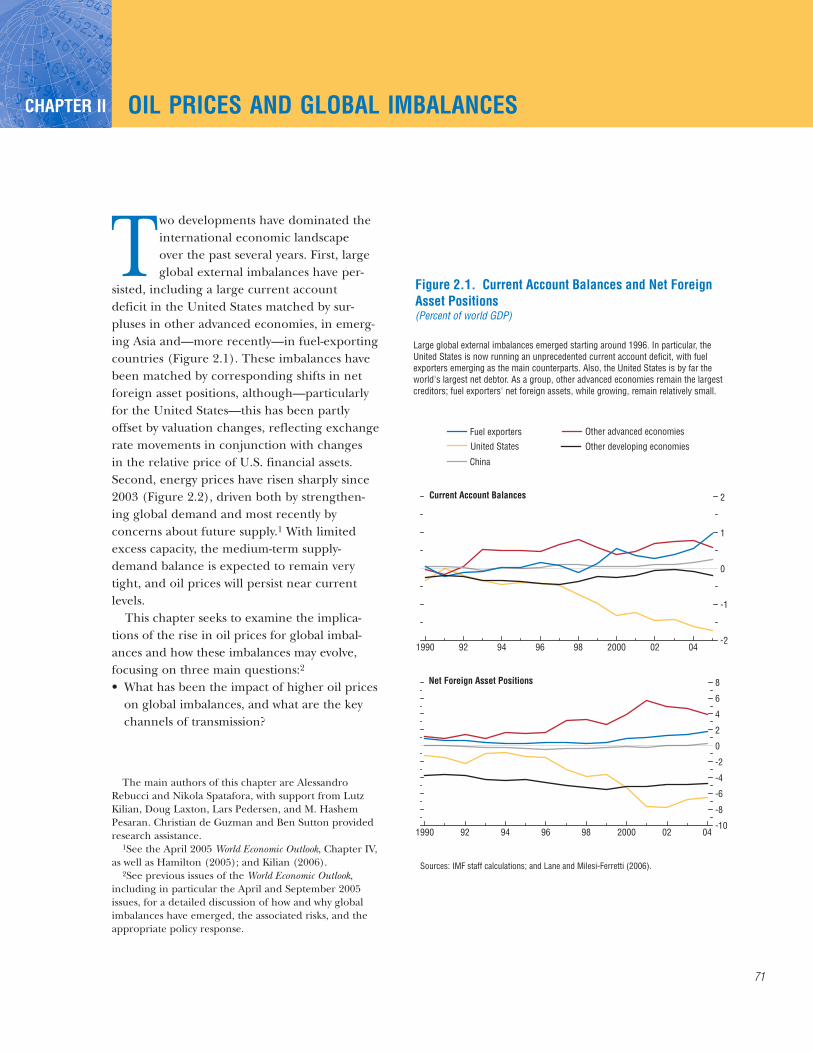
Figure 2.1. Current Account Balances and Net Foreign Asset Positions(Percent of world GDP)

Large global external imbalances emerged starting around 1996. In particular, the United States is now running an unprecedented current account deficit, with fuel exporters emerging as the main counterparts. Also, the United States is by far the world's largest net debtor. As a group, other advanced economies remain the largest creditors; fuel exporters' net foreign assets, while growing, remain relatively small.

Fuel exporters Other advanced economies

United States Other developing economies

China

Sources: IMF staff calculations; and Lane and Milesi-Ferretti (2006).

Current Account Balances

Net Foreign Asset Positions

The main authors of this chapter are AlessandroRebucci and Nikola Spatafora, with support from LutzKilian, Doug Laxton, Lars Pedersen, and M. HashemPesaran. Christian de Guzman and Ben Sutton providedresearch assistance.

1See the April 2005 World Economic Outlook, Chapter IV,as well as Hamilton (2005); and Kilian (2006).

2See previous issues of the World Economic Outlook,including in particular the April and September 2005issues, for a detailed discussion of how and why globalimbalances have emerged, the associated risks, and theappropriate policy response.

• How has the recycling of oil export revenues,or “petrodollars,” affected global and regionalfinancial markets?

• How do policy responses—in particular thepace at which oil exporters spend additionalrevenues, and the extent to which oilimporters allow pass-through of energy pricesinto core inflation—affect global and regionalsaving and investment, and hence the evolu-tion of external imbalances?Specifically, the next section documents key

facts about the energy market, external imbal-ances, and their financing, contrasting the cur-rent oil price shock with previous episodes. Thechapter then analyzes the likely impact of thecurrent shock on imbalances and how the imbal-ances may evolve over time. In particular, itoffers an econometric analysis of the historicalimpact of oil prices on external positions, thechannels of transmission, and the associatedadjustment process. It also investigates throughsimulations the impact of factors such as thespeed with which oil exporters spend their addi-tional revenues, and the extent to which oilprices are allowed to feed through into coreinflation.

How Does the Current Oil Price ShockCompare with Previous Episodes?

As a result of the almost $30 per barrelincrease in oil prices during 2002–05—and, to amuch lesser extent, rising production—globaloil exports have boomed. For a broad sample offuel exporters,3 the value of oil exports more


72

1970 75 80 85 90 95 2000 050

200

400

600

800Fuel Exporters' Net Oil Exports (billions of 2005 U.S. dollars)

0

20

40

60

80

100

120Real Oil Prices (2005 U.S. dollars a barrel)

Figure 2.2. Real Oil Prices and Net Oil Exports

Energy prices started to increase in 1999, with a sharp rise since 2003. This upsurge is to a large extent driven by growing demand in advanced and emerging economies, as well as by expectations of future market tightness. However, current and expected future real oil prices are still significantly below their value in the late 1970s and early 1980s.

Sources: IMF, International Financial Statistics; and IMF staff estimates.

1970 75 80 85 90 95 2000 05 07

3This sample consists of Algeria, Angola, Azerbaijan,Bahrain, Brunei Darussalam, Republic of Congo,Equatorial Guinea, Gabon, Islamic Republic of Iran, Iraq,Kazakhstan, Kuwait, Libya, Nigeria, Norway, Oman, Qatar,Russia, Saudi Arabia, Sudan, Syrian Arab Republic,Trinidad and Tobago, Turkmenistan, United ArabEmirates, Venezuela, and Yemen. The sample includes allthe countries in the World Economic Outlook “FuelExporters” analytical group as of February 2005, with theaddition of Kazakhstan and Norway. The main criteria forselection were that, over the past five years, the averageshare of fuel exports in total exports exceeds 40 percent;

than doubled to nearly $800 billion in 2005 andin real terms is now well above the previous1980 peak (Figure 2.2). For fuel exporters, thecurrent shock is in real terms comparable to (orindeed slightly larger than) the shocks of the1970s, although as a share of their GDP it is notquite as large (Table 2.1). Rising exports by fuelproducers have, of course, been matched by ris-ing imports elsewhere. The increase in the oil-import bill between 2002 and 2005 amounted toalmost 4 percent of GDP for China, and over 1percent of GDP for the United States, otheradvanced economies, and other developingcountries (Table 2.2). From the perspective ofthe global economy, nevertheless, the currentshock is smaller than in the 1970s, whethermeasured relative to world GDP, private capitalflows, or the size of financial markets (Table2.1). It is also worth noting that external imbal-ances were apparent well before oil pricesstarted to edge upwards in 1999, and certainlybefore oil prices reached their current peaks(Figure 2.3). That said, over the past two yearshigher oil prices account for one-half of the

deterioration in the U.S. current accountdeficit.

Since 2002, fuel exporters have spent a some-what smaller share of their additional revenuesthan after the first oil price shock. Their importsover the past few years have remained broadlyconstant as a share of GDP; even in absoluteterms, the increase in imports accounts for littlemore than one-half of the additional revenues(as opposed to the three-quarters share observedin the early 1970s). A more formal statisticalanalysis (see Box 2.1, “How Rapidly Are OilExporters Spending Their Revenue Gains?”)confirms these broad conclusions, while finding

HOW DOES THE CURRENT OIL PRICE SHOCK COMPARE WITH PREVIOUS EPISODES?

73

Table 2.1. Increase in Fuel Exporters’ Net Oil Exports1

(Billions of constant 2005 U.S. dollars, unless otherwise noted)

Percent of World Trade-Price- Percent of Percent of Percent of World Stock Market

CPI-Deflated Deflated2 World GDP3 Own GDP3 Private Capital Flows3 Capitalization3

1973–81 436 289 1.9 48.9 78.6 7.61973–76 239 139 1.1 27.8 58.4 5.51978–81 218 174 0.8 14.5 39.3 4.5

2002–05 437 382 1.2 33.2 37.3 1.6

Sources: IMF staff calculations, World Economic Outlook, International Financial Statistics; and World Bank, Financial Structure and EconomicDevelopment Database.

1All values deflated by the U.S. CPI, except where otherwise noted.2Trade-price-deflated figure is calculated using a trade-weighted average of the G-7 non-oil export-price deflator.3World GDP, own GDP, private capital flows, and stock market capitalization are all computed for the first year of the relevant period (except

for private capital flows and stock market capitalization during 1973–76 and 1973–81, when the final year of the relevant period was usedinstead, reflecting limited data availability). Private capital flows are defined as the sum of net direct investment, portfolio investment, and otherinvestment, from the balance of payments. Russia is excluded from all calculations in the “Percent of Own GDP” column, since it was not amarket economy during 1973–81.

Table 2.2. Change in Net Oil Exports, 2002–05

Billions ofConstant 2005 Percent of Percent of U.S. Dollars1 World GDP2 Own GDP2

Fuel exporters3 437 1.24 33.2United States –124 –0.35 –1.1Other advanced

economies4 –198 –0.56 –1.3China –53 –0.15 –3.8Other developing

countries5 –53 –0.15 –1.2

Source: IMF staff calculations.1All values deflated by the U.S. CPI.2Both world GDP and own GDP are computed for 2002.3Includes all the countries in the World Economic Outlook group

of fuel exporters, with the addition of Kazakhstan and Norway.4Includes all the countries in the World Economic Outlook group

of advanced economies, except for the United States.5Includes all other countries.

and the average value of fuel exports exceeds $500 mil-lion. Kazakhstan was included even though data were notavailable to gauge whether the first criterion was met. Thesample excludes large oil producers for which oil is not akey export earner, such as Canada, Ecuador, Mexico, andthe United Kingdom.

significant differences across countries (spend-ing rates are relatively low in CooperationCouncil of the Arab States of the Gulf, or GCC,countries, but considerably higher in the IslamicRepublic of Iran). In particular, the public sectorhas been cautious about rapidly ramping upspending: between 2002 and 2005, governmentbudget surpluses in fuel exporters increased onaverage by 11 percentage points of GDP. Thisappears to reflect concerns, fueled by past expe-rience, about whether such large amounts canbe spent effectively within a short period, andwhether the current oil price shock may provetransitory (see also IMF, 2005).

Will the shock in fact persist? From a histori-cal perspective, about one-half of the 1973–74oil price shock proved enduring, while the1979–81 shock was eventually completelyreversed. While any long-run oil price forecast issubject to enormous uncertainty, both marketexpectations and an assessment of medium-termoil market fundamentals suggest that a consider-able proportion of the recent shock will be per-manent in nature (see Chapter IV of the April2005 World Economic Outlook). Examining thisissue from a different perspective, the shock haschanged not just current income, but alsowealth: the value of fuel exporters’ petroleumreserves increased by more than $40 trillionbetween 1999 and 2005 (Table 2.3). If two-thirdsof this were to prove permanent in nature,broadly consistent with the estimates in the April2005 World Economic Outlook, it would imply an$850 billion increase in permanent income,4

almost three times the observed increase inaggregate imports to date. That said, theincrease in wealth has been spread very unevenlyacross fuel exporters; in some, such as Norwayand Bahrain, the value of total petroleumreserves is equivalent to current GDP or less.

Fuel exporters’ spending patterns are likelyto affect the relative demand for goods from


74

1999 2000 01 02 03 04 05-500

0

500

1000

1500

2000

1999 2000 01 02 03 04 05-500

0

500

1000

1500

2000

74 75 76-100

0

100

200

300

400

500

600

Figure 2.3. Fuel Exporters' Cumulative Current Account Balances and Capital Flows(Billions of 2005 U.S. dollars, cumulative)

Current account surpluses in the 1970s were associated with significant increases in official reserves and bank deposits. During the past few years, there has been relatively little accumulation of bank deposits, while portfolio investment flows have been sizable.

19

Source: IMF staff calculations. Cumulative, starting from 1974. Cumulative, starting from 1979. Cumulative, starting from 1999.

1

32

1974–76 1

79 80 81-100

0

100

200

300

400

500

600

7001979–812

1999–20053

19

1

Other investment, netPortfolio investment, netDirect investment, netReserve assets

Errors & omissions Current account

4Assuming a U.S. long-term real interest rate of 3 per-cent, roughly the average value observed over the past30 years.

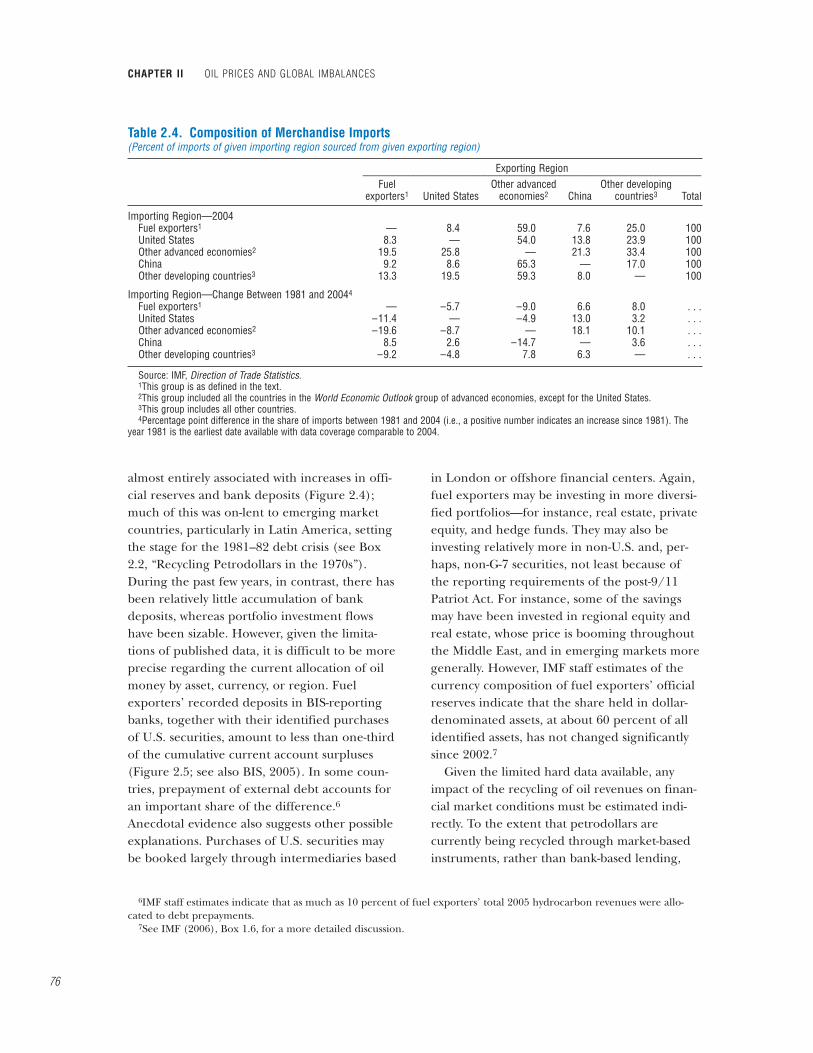
different regions. In particular, fuel exportersare importing fewer goods, measured as ashare of their total merchandise imports, fromthe United States today than they were in the1970s. In terms of market share of imports, theUnited States ranks well below either advancedeconomies or most developing economies(Table 2.4).5 Hence, as the shock redistributesincome from advanced economies and otherdeveloping countries toward fuel exporters, rel-ative demand for U.S. goods declines. Evenassuming that fuel exporters spend all their

incremental revenues, this “third-country” effectwould still act to increase the U.S. currentaccount deficit by a further $25 billion, or0.2 percent of GDP.

For now, however, oil exporters are saving aconsiderable share of their income. This raisesthe question of how the surplus funds are beingrecycled and how they are affecting globalfinancing conditions, including the extent towhich they are contributing to low global inter-est rates. At a broad level, the current accountsurpluses of the 1970s and early 1980s were

HOW DOES THE CURRENT OIL PRICE SHOCK COMPARE WITH PREVIOUS EPISODES?

75

Table 2.3. Petroleum Reserves

Change in Value of Reserves, Value of Reserves 1999–2005 Percent of___________________________

Percent of in Percent of Percent of Percent of World CrudeWorld Reserves 2005 GDP1 2005 GDP 2005 world GDP Oil Production

Sample of selected fuel exporters 88.2 2,156 1,763 98.3 62.4Kuwait 8.3 8,178 6,708 10.5 3.0Libya 3.3 5,847 5,034 4.3 2.0Saudi Arabia 22.1 4,722 3,856 27.6 13.2Kazakhstan 3.3 4,145 3,663 4.5 1.6United Arab Emirates 8.2 4,129 3,368 10.3 3.3Iran, I. R. of 11.1 3,679 3,199 14.8 5.1Venezuela 6.5 3,329 2,724 8.1 3.7Azerbaijan 0.6 3,276 2,672 0.7 0.4Qatar 1.3 2,244 2,143 1.9 1.2Nigeria 3.0 2,111 1,862 4.0 3.1Angola 0.7 1,826 1,672 1.0 1.2Congo, Rep. of 0.2 1,729 1,425 0.2 0.3Gabon 0.2 1,416 1,123 0.2 0.3Sudan 0.5 1,290 1,280 0.8 0.4Equatorial Guinea 0.1 1,133 1,042 0.2 0.4Oman 0.5 1,033 849 0.6 1.0Yemen 0.2 1,010 995 0.4 0.5Brunei Darussalam 0.1 927 761 0.1 0.3Syrian Arab Republic 0.3 661 572 0.4 0.7Algeria 1.0 635 522 1.3 2.4Russia 6.0 529 454 8.0 11.6Trinidad and Tobago 0.1 399 354 0.1 0.2Norway 0.8 185 144 1.0 4.0Turkmenistan — 175 142 0.1 0.3Bahrain — 53 36 — 0.1Iraq2 9.7 — — 12.1 2.5

OPEC 74.9 3,601 2,997 95.3 41.0World 100.0 153 128 128.0 100.0

Sources: BP, Statistical Review of World Energy 2005; Energy Information Administration; and IMF staff calculations. Note: Estimates of reserves refer to end-2004 and of crude oil production to 2004 (except for Bahrain, where production estimates refer to

2003).1Total value of stock of reserves calculated using average petroleum spot price for December 2005.2No GDP data available.

5As a caveat, the data reflect the composition of merchandise trade alone. However, there is anecdotal evidence that fuelexporters may be relatively large consumers of U.S. financial services.

almost entirely associated with increases in offi-cial reserves and bank deposits (Figure 2.4);much of this was on-lent to emerging marketcountries, particularly in Latin America, settingthe stage for the 1981–82 debt crisis (see Box2.2, “Recycling Petrodollars in the 1970s”).During the past few years, in contrast, there hasbeen relatively little accumulation of bankdeposits, whereas portfolio investment flowshave been sizable. However, given the limita-tions of published data, it is difficult to be moreprecise regarding the current allocation of oilmoney by asset, currency, or region. Fuelexporters’ recorded deposits in BIS-reportingbanks, together with their identified purchasesof U.S. securities, amount to less than one-thirdof the cumulative current account surpluses(Figure 2.5; see also BIS, 2005). In some coun-tries, prepayment of external debt accounts foran important share of the difference.6

Anecdotal evidence also suggests other possibleexplanations. Purchases of U.S. securities maybe booked largely through intermediaries based

in London or offshore financial centers. Again,fuel exporters may be investing in more diversi-fied portfolios—for instance, real estate, privateequity, and hedge funds. They may also beinvesting relatively more in non-U.S. and, per-haps, non-G-7 securities, not least because ofthe reporting requirements of the post-9/11Patriot Act. For instance, some of the savingsmay have been invested in regional equity andreal estate, whose price is booming throughoutthe Middle East, and in emerging markets moregenerally. However, IMF staff estimates of thecurrency composition of fuel exporters’ officialreserves indicate that the share held in dollar-denominated assets, at about 60 percent of allidentified assets, has not changed significantlysince 2002.7

Given the limited hard data available, anyimpact of the recycling of oil revenues on finan-cial market conditions must be estimated indi-rectly. To the extent that petrodollars arecurrently being recycled through market-basedinstruments, rather than bank-based lending,


76

Table 2.4. Composition of Merchandise Imports(Percent of imports of given importing region sourced from given exporting region)

Exporting Region___________________________________________________________________Fuel Other advanced Other developing

exporters1 United States economies2 China countries3 Total

Importing Region—2004Fuel exporters1 — 8.4 59.0 7.6 25.0 100United States 8.3 — 54.0 13.8 23.9 100Other advanced economies2 19.5 25.8 — 21.3 33.4 100China 9.2 8.6 65.3 — 17.0 100Other developing countries3 13.3 19.5 59.3 8.0 — 100

Importing Region—Change Between 1981 and 20044

Fuel exporters1 — –5.7 –9.0 6.6 8.0 . . .United States –11.4 — –4.9 13.0 3.2 . . .Other advanced economies2 –19.6 –8.7 — 18.1 10.1 . . .China 8.5 2.6 –14.7 — 3.6 . . .Other developing countries3 –9.2 –4.8 7.8 6.3 — . . .

Source: IMF, Direction of Trade Statistics.1This group is as defined in the text.2This group included all the countries in the World Economic Outlook group of advanced economies, except for the United States.3This group includes all other countries.4Percentage point difference in the share of imports between 1981 and 2004 (i.e., a positive number indicates an increase since 1981). The

year 1981 is the earliest date available with data coverage comparable to 2004.

6IMF staff estimates indicate that as much as 10 percent of fuel exporters’ total 2005 hydrocarbon revenues were allo-cated to debt prepayments.

7See IMF (2006), Box 1.6, for a more detailed discussion.

any effect on financing should be concentratedon market-based financial systems and on tradedassets. Box 2.3 (“The Impact of Petrodollars onU.S. and Emerging Market Bond Yields”) ana-lyzes whether the recycling of petrodollars hashelped lower either U.S. long-term interest ratesor emerging market spreads. There is indeedstrong evidence that capital inflows from abroadhave helped reduce yields on U.S. bonds. Theprecise impact of oil-related flows is more diffi-cult to disentangle, although its magnitude islikely to be relatively modest (at most a !/3 per-centage point reduction in U.S. nominal yieldsin 2005), possibly reflecting the diminishedimportance of fuel exporters in the internationalfinancial system.8

Finally, it is worth underscoring that thecurrent increase in oil prices is taking place ina very different global environment from thepast. In particular, the pattern of external imbal-ances has changed markedly since the 1970s.Then, large external deficits were concentratedin oil-importing developing countries (Figure2.3). Now, it is the United States that is runninga large external deficit, aggravated by high oilprices; given the central role of the UnitedStates in the world economy, this must heightenconcerns. Set against this, the nature of theinternational financial system has been trans-formed over time, with bank-based lendingbeing largely replaced by intermediationthrough financial markets. Now that the recy-cling of petrodollars is market-based and lessdriven by a few large intermediaries, it maywell prove more sustainable than in earlierepisodes.

How Will the Current Oil Price ShockAffect Global Imbalances?

The previous section sought to place therecent oil shock in context. This section looks in

HOW WILL THE CURRENT OIL PRICE SHOCK AFFECT GLOBAL IMBALANCES?

77

1999 2000 01 02 03 04-100

0

100

200

300

400

500

600

700

800

900

Figure 2.4. Fuel Exporters' Cumulative Current Account Balances and Identified Asset Purchases(Billions of U.S. dollars, cumulative since 1999)

In contrast to the 1970s, tracking the precise assets and countries into which oil revenues have been invested over the past few years is difficult. Identified purchases only account for a small share of current account surpluses.

Sources: Bank for International Settlements; Treasury International Capital System; and IMF staff calculations.

U.S. corporate bondsU.S. agency bondsU.S. treasuriesU.S. equities

Offshore bank deposits Current account balance

8Their gross external assets as of end-2004 accountedfor less than 4 percent of the world total, while theirshare of official reserves was about 10 percent.

more detail at how the global economy—andparticularly global imbalances—are likely toadjust. Following the initial oil price shock,adjustment takes place broadly as follows.9

• In fuel importers, the rise in world oil pricesworsens the trade balance, leading to a highercurrent account deficit and a deteriorating netforeign asset position. At the same time,higher oil prices tend to decrease private dis-posable income and corporate profitability,reducing domestic demand; along with adepreciation of the exchange rate, this acts tobring the current account back into equilib-rium over time. The speed and output cost ofadjustment depends on factors such as thedegree of trade openness, structuralflexibility,10 and central bank credibility, aswell as the shock’s expected persistence andthe speed with which it is allowed to feedthrough into domestic fuel prices. Amongother things, these determine the extent towhich rising oil prices raise inflationary pres-sures, necessitating a monetary tightening thatcould lead to a more pronounced slowing ingrowth.

• In fuel exporters, the process works broadly inreverse: trade surpluses are offset by strongergrowth and, over time, real exchange rateappreciation. One important difference, how-ever, is that fuel exporters may take longerthan fuel importers to adjust to the increase infuel prices.11 Hence, their savings may remainat high levels for extended periods.

• Consequently, aggregate global demand is likelyto fall. In turn, this sets in train a process ofmultilateral adjustment, driven by interestand exchange rate changes, as well as growth


78

Figure 2.5. Current Account and Oil Trade Balances(Percent of GDP)

In the 1970s, large external deficits, financed by the recycling of petrodollars, were concentrated in oil-importing developing countries. In recent years, the oil price shock has instead contributed to a widening U.S. current account deficit and has redistributed current account surpluses from other advanced economies and emerging Asia toward fuel exporters.

Source: IMF staff calculations.

Current account Oil trade balance

United States

1970 75 80 85 90 95 2000 05-8

-6

-4

-2

0

2Other Advanced Economies

1970 75 80 85 90 95 2000 05-6

-4

-2

0

2

4

6

8

1970 75 80 85 90 95 2000 05-6

-5

-4

-3

-2

-1

0

1 Other Developing EconomiesChina

Fuel Exporters

1970 75 80 85 90 95 2000 05-10

0

10

20

30

40

1970 75 80 85 90 95 2000 05-5

-4

-3

-2

-1

0

1

2

3

9See Ostry and Reinhart (1992) and Cashin andMcDermott (2003) for a detailed discussion of the inter-national transmission of terms-of-trade shocks.

10See the April 2005 World Economic Outlook, Chapter III.11The rise in oil exporters’ revenues is often very large

as a share of own GDP, and cyclical and/or structural andinstitutional constraints can make it very difficult toexpand demand quickly and efficiently. In contrast, nosuch constraints prevent demand from rapidly adjustingdownward in fuel importers.


79

Oil-exporting countries’ export revenueshave increased significantly over the past twoyears, with Organization of the PetroleumExporting Countries (OPEC) revenues esti-mated at about $500 billion in 2005, twice thatin 2003, but lower as a share of world GDP(1.1 percent) than both in 1974 and in 1979(around 2 percent). Oil exporters’ response tohigher revenues has an important bearing onthe evolution of global imbalances, as well astheir domestic economic developments. Thisbox assesses the response of major oil-exportingcountries’ imports to higher oil revenues andcompares it with their past behavior, in par-ticular with the 1970s’ episodes of sharpincreases in oil prices. To this end, it augmentsthe use of the simple marginal propensities toimport by a more formal estimation of importfunctions.

One might expect that after years of low oilprices and limited social expenditures in manyoil-exporting countries, spending would adjustrapidly to higher prices, especially in countrieswith large populations (relative to their oilincome) and sizable development needs. Inthe 1970s, however, oil exporters took time torespond to higher revenues, but once spendingtook off, it gradually rose to unsustainablelevels, with the average propensity to importsurpassing one by the late 1980s—reflecting inlarge part badly planned or wasteful projectsand declining oil prices. Spending was finallycurtailed (with the average propensity toimport falling below one) by the mid-1990s,after years of low oil prices, suggesting thatoil exporters must have initially assumed ahigher permanent component in the pricehikes than was justified ex post. The experiencewith the resulting fiscal deficits, therefore,could result in a more cautious use of higheroil revenues this time around, especially incountries where the ability to absorb theincreased revenues is limited.

A quantitative analysis and comparison ofspending patterns across the three episodes isnot straightforward in part because muchdepends on the time periods used and defini-tions of spending out of oil revenues. Forexample, a casual examination of the firstfigure—which depicts nominal imports and oilexports of OPEC countries—suggests thatspending out of oil revenues has been larger inthe current episode than in the past. Specifi-cally, in 2004 imports constituted about 90 per-cent of oil exports, in contrast to 38 percent in1974 and 75 percent in 1979.

However, more meaningful than these simpleratios is the behavior of the marginal propensityto import out of oil revenues over the shockperiods. There is no single correct way of defin-ing this propensity. One possible definition is

Box 2.1. How Rapidly Are Oil Exporters Spending Their Revenue Gains?

OPEC Imports and Oil Exports(Billions of U.S. dollars)

1970 75 80 85 90 95 2000 050

100

200

300

400

500

600

Sources: World Integrated Trade Solution; Source OECD; and IMF staff calculations. OPEC-9, excluding Iraq and Indonesia; data for United Arab Emirates start from 1971.

1

1

Value of imports of goods and services

Value of oil exports

Note: The main authors of this box are PelinBerkmen and Hossein Samiei.


80

the change in the current account over thechange in oil revenues.1 The results, shown inthe table, suggest that OPEC is currently spend-ing 24 percent of its additional oil revenues onimports. The figure is 31 percent for major non-OPEC countries and 15 percent for the Coope-ration Council of the Arab States of the Gulf(GCC). The latter group also appears to bespending less rapidly than in most past episodes,while for OPEC the picture is less clear-cut.These results, however, could underestimatespending propensities if, in particular, additionsto non-oil export revenues are also mostly oil-related (e.g., natural gas and oil products—as inmany OPEC countries), although the extentthat this may be the case is difficult to knowgiven data deficiencies. If the above definition ismodified to incorporate the change in non-oilrevenues too, then the marginal propensity tospend in the recent period will be higher (and

less different from past episodes). The figure forthe GCC (34 percent) is also now close to thatfor OPEC (36 percent). These aggregate trendsalso mask important differences across coun-tries. In particular, countries with larger popula-tions and/or expenditure needs, such as theIslamic Republic of Iran, Mexico, and Venezuelahave higher propensities to import than SaudiArabia and most other GCC members.

The above analysis, while informative, doesnot capture the impact of other variables onimports. As an alternative—and more formal—statistical analysis, we estimate import functionsfor the 1970–2001 period and examine the out-of-sample forecasts for the recent period. Thisprocedure does not distinguish shock episodesfrom other periods and focuses on testingwhether current performance is similar to the

Box 2.1 (concluded)

Marginal Propensity to Import Out of Oil Revenues1

1973– 1973– 1978– 1978– 2003–1974 1975 1980 1981 2005

GCC2 0.08 0.34 0.18 0.25 0.15OPEC3 0.14 0.52 0.24 0.42 0.24

Iran, I.R. of 0.17 0.68 0.35 0.24 0.37Saudi Arabia 0.01 0.32 0.27 0.39 0.26Venezuela 0.18 0.65 –0.15 0.01 0.46

Major non-OPEC4 . . . . . . . . . . . . 0.31Russia 0.77 1.37 0.76 1.08 0.20Norway . . . . . . 0.18 –0.30 –0.13Mexico . . . . . . . . . . . . 0.78

Sources: World Integrated Trade Solution; OECD; WorldEconomic Outlook; and IMF staff calculations.

1Defined as (change in imports net of non-oil exports, invest-ment income, and transfers)/(change in oil exports).

2The Cooperation Council of the Arab States of the Gulf(GCC) includes Bahrain, Kuwait, Oman, Qatar, Saudi Arabia, andthe United Arab Emirates.

3OPEC-9, excluding Iraq and Indonesia. Data for the UnitedArab Emirates start from 1971.

4Major non-OPEC includes Angola, Canada, Kazakhstan,Mexico, Norway, Oman, and Russia.

1Or equivalently: (change in imports net of non-oilexports, investment income, and transfers)/(changein oil exports). This definition assumes that theincrease in oil income is the only “shock” to externalrevenues and that additions to other revenues are fullyspent on imports.

1972 79 86 93 20001

2

3

4

5

6

1972 79 86 93 20001

1.5

2

2.5

3

3.5

4

4.5

5

Dynamic Forecasts for Real Imports(Log of billions of 2000 U.S. dollars)

Source: IMF staff estimates.

Forecast Actual

1972 79 86 93 20002.0

2.5

3.0

3.5

4.0

4.5Saudi ArabiaIran, I.R. of

1972 79 86 93 20001.5

2.0

2.5

3.0

3.5

4.0

4.5GCCOPEC

differentials. The incipient excess of globalsaving over investment puts downward pres-sure on real interest rates, which supportsinvestment demand in fuel importers andweakens incentives to save in fuel exporters.At the same time, exchange rate changes andgrowth differentials shift aggregate demandfrom importers to exporters.

• Adjustment is also influenced importantly byfinancial market developments. Higher oil priceswill tend to reduce asset prices—includingequities and exchange rates12—in oil-import-ing countries and to raise them in oil-export-ing countries. This will tend to reinforce theadjustment process, particularly in countries—such as the United States—where wealtheffects are large. In addition, changes in assetprices have important valuation effects.13 Forexample, if oil exporters hold equities or

bonds in oil-importing countries, their gainsfrom higher oil prices may be partly offset bycapital losses on their asset holdings, as stockmarkets in oil importers fall or their exchangerates depreciate.To investigate the adjustment process in more

detail, IMF staff used two separate but consistentvector autoregressions (VARs).14 The first ofthese, a standard VAR, investigates the linkbetween real oil prices and external positions(measured using both current accounts and netforeign assets) in the United States and inselected other country groups. The second, aGlobal VAR (GVAR),15 looks in more detail atthe link between oil prices, growth, inflation,and asset prices, to shed more light on how theadjustment takes place. Starting with the broadimplications of oil prices for external positions,the VARs suggest that:


81

average of the past. We use an error-correctionformulation, with real GDP and the terms oftrade as explanatory variables.2 The estimation isdone for oil-exporting countries individually, theGCC, and OPEC (for which comparison withthe past is possible). The results (second figure)suggest that OPEC’s spending is only slightlylower than that implied by its past behaviorwhile the GCC’s spending behavior is clearly

more conservative. Most of the individual coun-tries’ responses (e.g., the Islamic Republic ofIran and Saudi Arabia) are also consistent withtheir spending needs and with the trends in themarginal propensity to import discussed above.

On balance, these findings suggest that aver-age spending so far has been gradual, especiallyfor most GCC exporters. But expenditure needsare great in many countries and, based on the1970s experience, it is not at all certain that thecurrent trend will continue. The outcome willalso depend on perceptions about the magni-tude of the permanent component in higherprices. Higher spending, when prudent and onprojects with high returns, would help promotedomestic growth in these countries and con-tribute to reducing global imbalances.

2The logarithmic change in real imports is regressedon its lagged values, current and lagged values oflogarithmic changes in GDP and the terms of trade,and an error correction term. The estimation is car-ried out using an autoregressive distributed lag model,and employs the Schwarz-Bayesian criterion for lagselection.

12Bond prices will also fall, as long as nominal interest rates increase.13See the April 2005 World Economic Outlook, Chapter III, for a detailed discussion of valuation effects.14Adopting two separate but consistent models allows for more parsimonious specifications. The results are consistent

with those obtained combining the two models within a single GVAR.15As estimated by Dees and others (forthcoming); see Appendix 2.1 for details.

• Oil price shocks have a marked but relativelyshort-lived impact on current accounts(Figure 2.6).16 A permanent increase in realoil prices of $10 per barrel was on averageassociated with an increase in fuel exporters’current account surplus of about 2 percent ofown GDP, with the effect dying out withinthree years. This was matched by higherdeficits in the United States (about !/4 percentof GDP), other advanced economies, anddeveloping economies other than China.17

Among these, the impact on the UnitedStates was statistically the most significant aswell as persistent (with a half-life of aboutthree years).

• Oil price shocks also have a noticeable—andpredictable—effect on the net foreign assetposition of all regions, except the UnitedStates (see Figure 2.6). A permanent $10 perbarrel oil price shock boosts the net foreignasset position of oil exporters by about 2 per-cent of GDP, in line with the increase in thecurrent account; the increase has a half-life ofabout five years. More surprisingly, the esti-mated change in U.S. net foreign assets waspositive (although statistically insignificant),while other countries experienced a largerand more persistent reduction in net foreignassets than implied by the (cumulative)impact on the current account.18 This mayreflect the valuation effects described above,with declines in asset prices in the UnitedStates reducing wealth in the rest of theworld.Against this background, how does the under-

lying adjustment to an oil shock occur, and arethere significant differences across countries andregions? Figure 2.7 compares the adjustmentprocess across regions in response to a perma-


82

0 2 4 6 8 10-1.0

-0.5

0.0

0.5

1.0

0 2 4 6 8 10-1.0

-0.5

0.0

0.5

1.0

0 2 4 6 8 10-1.0

-0.5

0.0

0.5

1.0

0 2 4 6 8 10-1.0

-0.5

0.0

0.5

1.0

Other Advanced Economies

0 2 4 6 8 10-3.0

-1.5

0.0

1.5

3.0

0 2 4 6 8 10-3.0

-1.5

0.0

1.5

3.0

Current Account Response Net Foreign Asset Response

Fuel Exporters 2

0 2 4 6 8 10-1.0

-0.5

0.0

0.5

1.0

0 2 4 6 8 10-1.0

-0.5

0.0

0.5

1.0

0 2 4 6 8 10-1.0

-0.5

0.0

0.5

1.0

Other Developing Economies 4

United States

Source: IMF staff calculations. Response to a permanent $10 a barrel annual average increase in oil prices (measured in constant 2005 U.S. dollars). Fuel exporters' response presented on a wider scale. Net foreign asset data available only after 1980.

China3

Figure 2.6. Impact of Oil Price Shocks on External Imbalances, 1972–2004(Percent of GDP, x-axis in years)

1

1

32

4

In the short term, oil price shocks lead to external imbalances. However, the impact on net foreign assets has historically proved transitory.

95 percent error bandsPoint estimate

Error bands partially out of scale.

16See Appendix 2.1 for a fuller discussion of the identi-fication and interpretation of the oil price shock.

17China was a net oil exporter during the first half ofthe sample period.

18For many fuel exporters, complete data on foreignasset positions are not available. This may explain the sim-ilarity between the cumulative current account responseand the estimated change in net foreign assets.


83


United States ChinaFuel Exporters2

Figure 2.7. Adjustment to Oil Price Shocks, 1979:Q2–2003:Q4(Percent unless otherwise indicated, x-axis in quarters)

1

0 4 8 12 16 20 24-6

-3

0

3

6

0 4 8 12 16 20 24-6

-3

0

3

6

0 4 8 12 16 20 24-6

-3

0

3

6

0 4 8 12 16 20 24-2

-1

0

1

2

0 4 8 12 16 20 24-2

-1

0

1

2

0 4 8 12 16 20 24-2

-1

0

1

2Real Output

0 4 8 12 16 20 24-1.0

-0.5

0.0

0.5

1.0

0 4 8 12 16 20 24-1.0

-0.5

0.0

0.5

1.0

0 4 8 12 16 20 24-1.0

-0.5

0.0

0.5

1.0Long-Term Interest Rate6

0 4 8 12 16 20 24-10

-5

0

5

10

0 4 8 12 16 20 24-10

-5

0

5

10Real Equity Price 4

0 4 8 12 16 20 24-1.0

-0.5

0.0

0.5

1.0

0 4 8 12 16 20 24-1.0

-0.5

0.0

0.5

1.0

0 4 8 12 16 20 24-1.0

-0.5

0.0

0.5

1.0Inflation3

Real Exchange Rate5

Response to a permanent $10 a barrel annual average increase in oil prices (measured in constant 2005 U.S. dollars). Groups described in Appendix 2.1. Y-axis in percentage points at a quarterly rate. For other developing countries, error bands out of scale. For fuel exporters, data only available for Canada, Norway, and the United Kingdom. For other developing countries, confidence intervals partially out of scale. For China, insufficient data available. Error bands partially out of scale. For the United States, real effective exchange rate vis-à-vis other groups shown. For all other groups, CPI-based real bilateral exchange rate vis-à-vis the United States shown. Y-axis in percentage points at a quarterly rate; multiply by four to annualize. For other developing countries, only Korea and South Africa

1

32

4

5

6

Source: IMF staff calculations, based on Dees and others (forthcoming).

shown. For China, short-term interest rates shown.

nent oil price shock (again, of $10 per barrel).19

The key points are as follows.• The basic adjustment channels work broadly as

described above, with slowing growth and realdepreciation supporting the trade adjustmentin oil importers, while fuel exporters experi-ence real appreciation and output growth. Inparticular, in the United States, the real effec-tive exchange rate depreciates, and outputdeclines by up to !/2 percent, although thisdecrease is statistically weak. In other advancedeconomies, the exchange rate also depreciates,but any output declines are smaller than in theUnited States (especially in Japan).20

• Inflation in advanced economies rises after oneyear by an annualized #/4 percentage point inthe United States, and somewhat less else-where.21 This has historically been accompa-nied by an increase in both short- andlong-term nominal interest rates. Long-termreal rates, however, fall temporarily in responseto the shock. This helps support demand infuel importers and maintain the global saving-investment balance, until exchange ratechanges and growth differentials work theirway through the adjustment process. In devel-oping countries, the response of inflation can-not be estimated precisely, reflecting strongheterogeneity within this group.22


84

2

1

2

Figure 2.7 (concluded)


Other Advanced Economies Other Developing Economies

0 4 8 12 16 20 24-2

-1

0

1

2

0 4 8 12 16 20 24-2

-1

0

1

2

0 4 8 12 16 20 24-1.0

-0.5

0.0

0.5

1.0

0 4 8 12 16 20 24-1.0

-0.5

0.0

0.5

1.0Long-Term Interest Rate6

0 4 8 12 16 20 24-1.0

-0.5

0.0

0.5

1.0

0 4 8 12 16 20 24-1.0

-0.5

0.0

0.5

1.0Inflation3

Real Exchange Rate5

0 4 8 12 16 20 24-6

-3

0

3

6

0 4 8 12 16 20 24-6

-3

0

3

6

Real Output

0 4 8 12 16 20 24-10

-5

0

5

10

0 4 8 12 16 20 24-10

-5

0

5

10Real Equity Price4

Response to a permanent $10 a barrel annual average increase in oil prices (measured in constant 2005 U.S. dollars). Groups described in Appendix 2.1. Y-axis in percentage points at a quarterly rate. For other developing countries, error

For fuel exporters, data only available for Canada, Norway, and the United Kingdom. For other developing countries, confidence intervals partially out of scale. For China, insufficient data available. Error bands partially out of scale. For the United States, real effective exchange rate vis-à-vis other groups shown. For all other groups, CPI-based real bilateral exchange rate vis-à-vis the United States shown. Y-axis in percentage points at a quarterly rate; multiply by four to annualize. For otherdeveloping countries, only Korea and South Africa shown. For China, short-term interest rates shown.

1

32

4

5

6

bands out of scale.

19These results are based on the estimates of Dees andothers (forthcoming). For this exercise, both the sampleperiod (1979:Q2–2003:Q4) and the list of countriesincluded (see Appendix 2.1) are slightly different fromwhat was previously used. This reflects the limited avail-ability of the quarterly data needed to estimate the under-lying GVAR model.

20In Japan, there is a marked depreciation. In the euroarea, in contrast, the real exchange rate does not respond(see Appendix 2.1).

21For this sample, which includes the second oil priceshock and the associated delayed policy response, thehypothesis that inflation is affected even in the long runcannot be rejected.

22These results, while based on a different methodol-ogy, are broadly consistent with earlier IMF staff estimatesof the impact of an oil price shock. For instance, the cal-culations in IMF (2000) suggest that a $10 per barrelincrease in oil prices would reduce real GDP in theUnited States and euro area by about !/2 percent, andincrease inflation after one year by 1 percentage point.


85

The first “oil shock” began in the fall of 1973.The sudden tripling of world oil prices resultedin a large windfall gain for oil-exporting coun-tries at the expense of oil importers. It also ledto a major financial shock, since most exportingcountries spent only a small portion of theincreased revenues. In 1974, the first full yearafter the initial shock, the aggregate currentaccount surplus of major oil-exporting countriesamounted to $68 billion (one-third of theirGDP). The major counterparts were the deficitsof industrial countries ($31 billion, 0.8 percentof GDP) and of oil-importing developing coun-tries, or OIDC ($34 billion, 10!/2 percent of GDP).Although these shifts moderated over time as oilexporters adjusted to the new market situationwith increased spending, the general patternpersisted through the rest of the decade.1

Oil exporters faced the question of how to usetheir sizable current account surplus. Data onidentified investments, which account for almostthe entire surplus, indicate that most of themoney was channeled into a few well-established

markets. In 1974, more than half was placed inbank deposits and money market instruments(including short-term treasury securities) inadvanced economies (see the first table). Of theliquid investments in the United States, treasurysecurities accounted for less than a sixth of thetotal, with the rest placed mostly with commer-cial banks. About $25 billion was channeled intolong-term investments, such as loans to nationalgovernments and international agencies, as wellas government bonds in the United States andthe United Kingdom. Broadly speaking, the pat-tern persisted throughout the rest of the 1970s.

The financial shock from the oil priceincreases of the 1970s came at a time when thepotential for large private international capitalflows was just beginning to be realized. The firstrelevant development, which began in the late1960s, was the deregulation and consequentinnovative evolution of Eurocurrency markets.The oil shock of 1973–74 reinforced this devel-opment, providing new fuel for these markets bymaking large sums of liquid assets available forinvestment. By then, banks in Europe and in lessregulated “offshore” financial centers weremuch better prepared than they would havebeen even a few years earlier to accept andinvest dollar-denominated deposits and otherliquid liabilities. A third factor was weak aggre-

Box 2.2. Recycling Petrodollars in the 1970s

Fuel Exporters’ Deployment of Current Account Surpluses(Billions of U.S. dollars; by type of financial investment)

1974 1975 1976 1977 1978 1979

Bank deposits and money market investmentsDollar deposits in the United States 1.9 1.1 1.8 0.4 0.8 4.9Sterling deposits in the United Kingdom 1.7 0.2 –1.4 0.3 0.2 1.4Deposits in foreign currency markets 22.8 9.1 12.1 10.6 3.0 31.2Treasury bills in the United Kingdom and the United States 4.8 0.6 –1.0 –1.1 –0.8 3.4Total 31.2 11.0 11.5 10.2 3.2 40.9

Long-term investmentsSpecial bilateral arrangements 11.9 12.4 12.2 12.7 8.7 11.8Loans to international agencies 3.5 4.0 2.0 0.3 0.1 –0.4Government securities in the United Kingdom and

the United States 1.1 2.2 4.1 4.5 –1.8 –0.9Other1 9.7 6.1 8.5 5.8 3.3 2.4Total 25.1 24.7 26.8 23.3 10.3 12.9

Total new investments 56.3 35.7 38.3 33.5 13.5 53.8

Source: Bank for International Settlements.1Including equity and property investments in the United Kingdom and the United States, and foreign currency lending.

Note: The main authors of this box are James M.Boughton and Suchitra Kumarapathy.

1The current account balance of industrial countriesswung from a cumulative surplus of $23 billion in1968–73 to a deficit of $44 billion in 1974–79, while thecumulative deficit of OIDC doubled to $139 billion.


86

gate demand in industrial countries, whichmeant that banks in those countries had to findother profitable outlets for the “petrodollars”that oil exporters were investing with them. Formany banks, meeting this challenge meant mov-ing into new markets where loan demand wasstronger, including Latin America and otherdeveloping countries.

A large part of the initial response to the oilshocks took the form of official “recycling” ofpetrodollars, in which the IMF and other officialcreditors provided fast-disbursing loans toOIDC. The main vehicle for the IMF was an “OilFacility,” newly established in 1974, throughwhich $2.4 billion were lent to 45 developingcountries from 1974 to 1976. Because the shockwas thought to be temporary, this financing wasprovided with only token conditionality. Overall,in 1974–76, official recycling from multilateraland bilateral creditors and donors amounted to$48 billion, two-thirds of which was bilateral.

Over time, international private banks tookover much of the financing role. In 1975,long-term official loans and grants to OIDCamounted to about $18 billion, and privatefinancing was estimated at roughly the sameamount, most of it channeled through commer-cial banks. But cross-border private flows, espe-cially through banks, then increased sharply. Forinstance, the external foreign currency assetsreported by banks in eight European countries,Canada, Japan, the United States, and offshorebranches of U.S. banks quadrupled to almost$1 trillion between 1973 and 1980.2 The

Eurobond market also expanded considerably,with the total value of international and foreignbond issues growing from $12 billion in 1974 to$38 billion in 1980.

A portion of the recycled funds went toindustrial countries with large current accountdeficits, including France, Italy, and the UnitedKingdom, which relied on a combination ofofficial and private external financing (see thesecond table). In 1974, for instance, the UnitedKingdom financed its $7.5 billion currentaccount deficit by means of compensatory for-eign borrowing and direct inflows of funds fromoil-exporting countries (at the time, the UnitedKingdom was still developing the North Sea oilfields and was a major oil importer). The IMFalso provided financing to several industrialcountries, including large Stand-By Arrange-ments for Italy and the United Kingdom, in partbecause of the failure of these countries toadjust policies and aggregate demand fully tothe oil shock.

An even greater share of the recycled petro-dollars went to developing countries, many ofwhich had initially faced difficulties financingtheir increased current account deficits. Weakoverall aggregate demand and a big unantici-pated jump in price inflation kept world interestrates low in nominal terms and substantially

Box 2.2 (concluded)

Financial Inflows for Selected OECD Economiesin 1974(Billions of U.S. dollars)

Financial Inflows___________________________________Traditional Compensatory

capital foreign Officialinflows borrowing1 inflows2 Total

United Kingdom 2.2 4.13 3.24 9.5Italy 1.0 2.1 5.3 8.4France 3.8 1.7 0.5 6.0

Source: OECD, Economic Outlook, 1975.1Official or semi-official borrowing from foreign private

institutions.2Private and official borrowing from foreign official institutions.3Of which, $2.6 billion representing foreign currency borrow-

ing by the public sector under the exchange cover scheme, and$1.5 billion drawing on the government Euro-loan.

4Including an increase of $5.3 billion in sterling-denominatedexchange reserves by oil-exporting countries.

2Since the lion’s share of the recycling in the 1970spassed through the banking systems or securities mar-kets of industrial countries, the Bank for InternationalSettlements (BIS) was able to estimate the composi-tion and direction of financial flows, using dataobtained largely from its participating central banks.Subsequently, financial markets continued to globalizeand diversify into new and more complex instruments,and a variety of nonbank financial institutions becamemajor intermediaries for cross-border flows. Since themid-1990s the BIS has ceased reporting cross-borderbanking claims on a basis comparable to earlier years,and tracking the course of overall flows has becomemuch more difficult.

• There also appears to be an active valuationchannel. Equity prices fall by 2–4 percentagepoints in major advanced economies, which—along with the depreciation of the U.S.dollar—results in a wealth transfer to theUnited States from other economies.The analysis so far describes the average

impact of oil price shocks in the past. However,the effects of the current shock, including thespeed and nature of the future adjustmentprocess, may be different, and in particular willdepend on two policy-related factors. First, asnoted above, oil producers appear to be increas-ing their spending in response to higher rev-enues more slowly than in the past. In addition,as discussed in Chapter I, the impact of oilprices on core inflation to date has been surpris-ingly mild relative to previous experience, sothat central banks have not had to raise short-term interest rates to reduce inflationary pres-sures. Partly as a result, growth in oil-importingcountries has been relatively unaffected, imply-ing that trade balances may take longer toadjust; set against this, for net debtors, relativelylower interest payments on external debt havereduced any negative impact on currentaccounts.23

To examine the potential impact of thesevarious factors on the adjustment of globalimbalances, IMF staff undertook two simula-tions using the IMF’s MULTIMOD model.24

The first scenario assumes rapid adjustment inoil exporters, as compared to the WEO baselinewhere their existing current account surplusescontinue into the medium term. Specifically,the scenario assumes that imports by oilexporters increase by $150 billion in 2006(about !/3 of their aggregate 2005 currentaccount surplus, or !/3 percent of world GDP),and $350 billion (about #/4 of their currentsurplus) by 2010. This more rapid pace ofexpenditure shrinks the U.S. current accountdeficit, by almost #/4 percent of GDP by 2010,and also leads to some real dollar appreciation(Table 2.5). The decline in global savings resultsin an increase in real and nominal interest ratesin oil importers, amounting to up to 40 basispoints. There is little net impact on growth inadvanced economies.

In the second scenario, it is assumed that thelow level of pass-through into core inflation can-not be sustained and that pass-through picks upin 2006, although its magnitude is still only halfof what would have been expected based on his-


87

negative in real terms throughout the 1970s,encouraging developing countries to take onloans. For many developing countries that wereexporters of primary commodities, a commodity-price boom in the mid-1970s made their bor-rowing terms look even more attractive. Forinstance, in 1973–78 low-income countries as agroup paid an average nominal interest rate of

just over 3 percent on their external debt, whiletheir export prices—measured in the depreciat-ing U.S. dollar—rose at an average annual rateof 18 percent. Latin America emerged as thelargest borrowing region, accounting for two-thirds of total credits issued by reporting banksto OIDC—a development that laid the basis forthe debt crises of the 1980s.

23In addition, historical experience may prove misleading in illustrating the potential impact of any large future oil priceshock, if there are important nonlinearities in the effects of such shocks.

24For a description of MULTIMOD, see Laxton and others (1998); see Hunt, Isard, and Laxton (2001) for the specificversion employed here. MULTIMOD does not have a separate “oil exporters” group. The estimates reported aggregate allthose countries whose trade surplus increases in response to an oil price increase. This includes Canada, the UnitedKingdom, the “small industrial economies” group, and a group of high-income developing economies that are mainly oilexporters.

torical experience through 2003. As core infla-tion increases, central banks respond by increas-ing nominal interest rates significantly (byabout 70 basis points for the United States in2007, relative to the baseline), so as to containthe inflationary impact of the increase in energyprices (Table 2.6). In turn, higher interest ratesact to depress demand and output, with somepositive effects on the trade balance. Higherinterest rates also increase the interest burden

on the U.S. stock of net foreign liabilities,which tends to raise both the U.S. currentaccount deficit and the Japanese currentaccount surplus.25 Nevertheless, as long asmonetary policy responds promptly to the infla-tionary pressures, the effects on both outputand, especially, the current account are rela-tively mild. If the monetary policy response wereinstead delayed, the eventual effects wouldprove much more sizable.26


88

Table 2.5. Impact of Oil Price Shock: GreaterSpending by Fuel Exporters(Relative to baseline)

2006 2007 2008 2009 2010

Current account balance (in percent of GDP)

United States 0.4 0.4 0.5 0.6 0.7Japan 0.5 0.7 0.9 1.0 1.1Euro area 0.5 0.7 0.9 1.0 1.1

Core inflation (in percentage points)

United States 0.1 0.1 — — 0.1Japan 0.1 0.1 0.1 0.1 0.1Euro area 0.2 0.2 0.1 — 0.1

Real short-term interest rate (in percentage points)


Nominal short-term interest rate (in percentage points)


GDP (in percent)United States 0.5 0.1 –0.4 –0.2 –0.1Japan 0.5 0.2 –0.4 –0.3 –0.1Euro area 0.7 0.2 –0.5 –0.3 –0.1

Real effective exchange rate (in percent)

United States –0.8 –0.7 –0.6 –0.6 –0.6Japan 0.7 0.7 0.7 0.6 0.6Euro area –0.3 –0.3 –0.4 –0.4 –0.4


Table 2.6. Impact of Oil Price Shock: DelayedPass-Through to Core Inflation(Relative to baseline)

2006 2007 2008 2009 2010

Current account balance (in percent of GDP)

United States — — –0.1 –0.1 –0.1Japan — 0.1 0.2 0.2 0.1Euro area — — — — —

Core inflation (in percentage points)

United States 0.1 0.3 0.1 0.1 —Japan 0.1 0.3 0.1 — —Euro area 0.1 0.2 0.1 — —

Real short-term interest rate (in percentage points)

United States 0.2 0.6 0.4 0.3 0.2Japan 0.2 0.5 0.3 0.2 0.1Euro area 0.2 0.5 0.2 0.1 —

Nominal short-term interest rate (in percentage points)

United States 0.3 0.7 0.6 0.3 0.2Japan 0.3 0.6 0.4 0.2 0.1Euro area 0.2 0.6 0.3 0.1 —

GDP (in percent)United States –0.3 –0.8 –0.7 –0.5 –0.4Japan –0.2 –0.6 –0.6 –0.4 –0.3Euro area –0.2 –0.5 –0.5 –0.3 –0.2

Real effective exchange rate(in percent)

United States 0.1 0.3 0.3 0.2 0.1Japan — 0.1 — 0.1 0.1Euro area –0.1 –0.4 –0.3 –0.2 –0.2


25The impact on net foreign assets, however, would be mitigated by valuation effects working in favor of the UnitedStates but not present in the model.

26For technical reasons, all scenarios assume that the oil price is driven only by oil supply shocks. This tends to overesti-mate the positive impact of lower oil prices on real GDP in oil-consuming countries. However, there is no a priori reasonwhy the assumption should affect results for either scenario relative to the baseline. In addition, all scenarios assume fulland immediate pass-through of the world oil price into domestic oil prices. Incomplete pass-through would result in sloweradjustment.


89

How does the recycling of oil-export revenuesaffect global financial markets? To the extent thathigher oil prices increase world net savings, andthat saved petrodollars are used to purchase givensecurities, the outcome would be an increase inthe price of (or, equivalently, a lower interest rateon) such securities. In turn, this could lead to asecond-round effect on the price of other, similarsecurities. This box analyzes the issue by focusingon the link between oil prices and interest rateson U.S. and emerging market bonds.

Examining first the United States, direct evi-dence of a link between petrodollars, capitalinflows, and interest rates is not available, inlarge part because many oil exporters tend topurchase U.S. securities through third-countryintermediaries. Such third-country trades con-found the country attribution of U.S. capitalflows data. The estimation here therefore pro-ceeds more indirectly. As a first step, followingWarnock and Warnock (2006), there is evidencethat capital flows to the United States do putdownward pressure on U.S. interest rates (seethe first table, column 1). Foreign flows intoU.S. government securities in the 12-monthperiod through May 2005 depressed U.S. 10-yearyields by 86 basis points,1 controlling for factorssuch as inflation expectations and the federalfunds rate. On this basis, if one assumed thatfuel exporters used one half of their currentaccount surplus to finance investments in theUnited States, the increase in oil prices over thelast two years would have reduced U.S. yields byabout !/3 percentage point (holding constant allother capital flows).

To investigate the issue further, the Warnockand Warnock regression analysis was extendedby disaggregating total capital flows into theUnited States into two components: those attrib-utable to East Asian countries, which areunlikely to directly reflect oil-export revenues;

and all others (“Other Flows”).2 Perhaps surpris-ingly, East Asian inflows were found to have arelatively greater dollar-for-dollar impact on U.S.yields, although Other Flows have recently beensomewhat larger in absolute terms (see the firsttable, column 2). Among possible explanations,East Asian purchases may have been concen-trated on more thinly traded, longer-maturityportions of the yield curve, where purchaseshave a greater impact. In addition, interventionsby Asian central banks may have been inter-preted as a signal that they were likely to con-tinue buying dollars in the future.3 Overall, theregression attributes 52 basis points of the total

Box 2.3. The Impact of Petrodollars on U.S. and Emerging Market Bond Yields

The Impact of Oil Revenues on U.S. Interest Rates1

Nominal 10-Year Treasury Yield_________________________

(1) (2) (3)

Foreign capital inflows2,3 –0.24* . . . . . .East Asian flows . . . –0.42* –0.35*Other flows . . . –0.14* . . .Oil-related . . . . . . –0.12Residual . . . . . . –0.13*

Inflation expectations, 10-year ahead 0.63* 0.67* 0.65*

Interest rate risk premium 1.88* 3.16* 0.90*Federal funds rate 0.36* 0.33* 0.35*Structural budget deficit2 0.25* 0.23* 0.22*

R2 0.90 0.90 0.85

Source: Authors’ calculations.1The sample is monthly, from August 1987 to May 2005.

Yields are measured in percentage points. Asterisks denote sta-tistical significance at the 1 percent level. The following vari-ables are included but not reported: expected real GDP growth;the difference between 1-year ahead and 10-year ahead inflationexpectations; and a constant.

2Scaled by lagged GDP.3Twelve-month benchmark-consistent foreign official flows

into U.S. treasury and agency bonds.

Note: The main authors of this box are LauraKodres and Frank Warnock.

1Calculated as 12-month inflows, amounting to 3.65(percent of lagged GDP), times the estimated coeffi-cient, –0.236.

2For the purpose of this box, East Asia consists ofChina, Hong Kong SAR, Japan, Korea, and TaiwanProvince of China—countries and territories whosegovernments have recently accumulated substantialpositions in U.S. government securities.

3On a more technical note, “Other Flows” may alsocontain private flows that are related to other variablesin the regression. In contrast, East Asian flows are pri-marily official flows, and may more reasonably betreated as exogenous.


90

yield reduction between June 2004 and May2005 to East Asian flows, but only 34 basis pointsto Other Flows.

Of course, Other Flows cannot be entirelyassumed to reflect oil-export revenues—theyhave many potential sources. To isolate theeffect of oil revenues, Other Flows were explic-itly regressed on oil prices.4 In this regression,however, oil prices have very little explanatorypower. Further, the part of Other Flows that isrelated to oil prices does not help explain lowerU.S. rates, even though non-oil-related OtherFlows do have a statistically significant impact(see the first table, column 3).5

Summing up, while one might expect higheroil prices and the consequent recycling ofpetrodollars to exert downward pressure on U.S.interest rates, such an effect is hard to detect sta-tistically among all the competing influences onU.S. yields. This may well reflect the relativelylimited magnitude of petrodollar flows. Twocaveats should, however, be stressed. First, thesenegative findings in part likely reflect the lack ofdirect data on capital inflows from fuel-exportingcountries. Second, the above analysis treats U.S.interest rates as being determined separatelyfrom global interest rates. In an integrated worldcapital market, oil prices may also affect U.S.rates indirectly, through the impact of recycledpetrodollars on interest rates in other countries.That said, the regressions failed to find a statisti-cally significant impact of interest rate differen-tials or exchange rates on U.S. yields.6

Even if petrodollars have only a limited effecton the large U.S. bond market, they might havea more sizable impact on the smaller marketfor emerging market debt. This hypothesis isexplored next, using a model of emergingmarket bond spreads that controls for theimpact of country-specific and global macro-economic fundamentals and of variables relatedto U.S. financial markets. Specifically, themodel recognizes that oil prices (as well asnonfuel commodity prices, global industrialproduction, and U.S. interest rates) influenceemerging market bond spreads through twoseparate channels. First, oil prices affect emerg-ing market “fundamentals,” as proxied by theircredit ratings and outlooks, which in turn affecttheir spreads. In particular, for oil importers,higher oil prices may negatively affect the cur-

Box 2.3 (concluded)

Determinants of Emerging Market Bond Spreads

Explanatory Variable Coefficient1

Oil price2 0.005Non-fuel commodity prices2 –1.096*World industrial production2 –1.173Predicted credit ratings and outlooks3 0.237*

Federal funds three-month future rate 0.076*

R2 Within = 0.49;Between = 0.73; Overall = 0.64

Sources: Bloomberg, L.P.; The PRS Group; J.P. Morgan;Bloomberg; and authors’ calculations.

1Fixed-effects panel regression using 2,345 monthlyobservations on 29 countries, from January 1991 to May2005. The dependent variable is the log of Emerging MarketBond Spreads, measured in basis points, using the J.P. MorganEmerging Market Bond Indices (EMBI) relative to the U.S.10-year treasury bond. All countries for which EMBI areavailable are included, except that Algeria and Côte d’Ivoireare excluded owing to lack of other data; Russia and Venezuelaare excluded owing to significant oil exports; Nigeria isexcluded on both grounds; and Argentina is excluded owingto its crisis-related spreads in 2001. Asterisks denote sta-tistical significance at the 1 percent level. The followingvariables are included but not reported: expectations offederal funds rate (FF) increase; expectations of FF decrease;volatility of FF futures; volatility of FF futures × expectationsof FF increase; volatility of FF futures × expectations of FFdecrease; volatility of S&P 500 options; a constant; and atime trend.

2In logs.3Predicted value for default risk, from a separate first-stage

regression.

4Allowing for 24 monthly lags, and deflating bynominal GDP. An alternative specification alsoincluded oil-export revenues, as proxied by oil pricestimes fuel exporters’ total petroleum output, but thesedid not prove significant.

5Over selected subperiods (e.g., starting in January1999), there is a relationship between Other Flowsand oil prices. However, the portion of Other Flowsattributable to oil prices over such subperiods stilldoes not help explain U.S. rates.

6Their effect may already be picked up through otherincluded variables, such as inflationary expectations oroutput. In a similar vein, purchases of U.S. corporatesecurities by oil exporters might impact U.S. interestrates; this effect is again not explicitly modeled.

ConclusionsGlobal imbalances had emerged long before

the current oil price shock began. Neverthe-less, some of these imbalances have clearlybeen exacerbated by higher energy prices. Inparticular, the increase in oil prices since 2003has directly worsened the U.S. current accountdeficit by over 1 percent of GDP; at the sametime, higher oil prices have tended to reducesurpluses in non-oil-exporting developingcountries, notably in Asia. To the extent thathigher net savings by oil exporters have drivendown global interest rates, and that these lowerrates have boosted demand in economies withmarket-based financial systems, such as theUnited States, the oil price shock may also havehad an additional indirect negative effect onthe U.S. external position. Since it is neitherfeasible nor desirable for oil exporters to spendtheir newfound revenues immediately, globalcurrent account imbalances are likely to remainat elevated levels for longer than would other-wise have been the case, heightening the risk ofa sudden, disorderly adjustment.

In the past, current accounts have tended toadjust relatively quickly to oil shocks, as higherenergy prices led to a rise in interest rates, aslowdown in growth and domestic demand, andchanges in exchange rates and asset prices. Thistime, in part because of improved monetary

frameworks and credibility, the impact on short-term interest rates, growth, and inflation hasbeen smaller than before, while deeper finan-cial integration may facilitate the persistence ofdeficits. Further, authorities in fuel-exportingcountries are being somewhat more cautious inincreasing spending, even though marketexpectations indicate that the current energyprice shock is likely to prove more persistentthan in the 1970s. All this suggests that currentaccounts may adjust more slowly now than inthe past.

As with any terms-of-trade shock, much of theadjustment must take place in the private sector,but policies can also play an important support-ing role. For consuming countries, this requiresfull pass-through of world oil prices into domes-tic energy prices, accompanied by a monetarystance that guards against potential spilloversinto core inflation. For producers, most ofwhich are developing countries, the rise in oilrevenues represents a major developmentopportunity. While the pace at which oil earn-ings can be usefully spent will vary by country,measures to boost expenditures in areas wherereturns are high (as well as structural reforms toboost domestic supply, particularly of nontrad-ables) would be highly desirable both from adomestic perspective and to help reduce globalimbalances.

CONCLUSIONS

91

rent account, one of the variables used to estab-lish credit ratings.

Second, as discussed above, if a significantshare of oil exporters’ revenues is used to pur-chase emerging market debt , then higher oilprices may be associated with lower emergingmarket spreads. However, even after controllingfor fundamentals, estimates suggest that anylink between higher oil prices and lower emerg-ing market spreads becomes statisticallyinsignificant when industrial production is alsoincluded in the regressions (see the second

table). Oil prices and industrial productionboth move in sync with the global economiccycle, making their independent influence onspreads difficult to disentangle. Interestingly,nonfuel commodity prices do have a statisticallysignificant, negative impact on spreads. Eithertheir positive influence on fundamentals inthose nonfuel commodity exporters included inthe sample (such as Chile) is not sufficientlycaptured by credit ratings, or the associatedexport revenues are being used to purchaseemerging market debt.

Appendix 2.1. Oil Prices and GlobalImbalances: Methodology, Data, andFurther ResultsThe authors of this appendix are Alessandro Rebucciand Nikola Spatafora.

This appendix describes more fully the empir-ical evidence, presented earlier in this chapter,regarding the effects of oil price shocks onexternal imbalances and the associated adjust-ment process. Specifically, the appendixdescribes the econometric models and data usedand the identification of the oil price shocks. Italso reports additional results underlying theaggregate responses depicted in Figure 2.7.

The Econometric Models

The econometric models used to analyze theresponse to oil price shocks of the currentaccount or net foreign assets (NFA) are standardVARs, which include one lag of the followingendogenous variables:27

• The real oil price, defined as the averageannual nominal oil price deflated by the U.S.CPI, in first-difference form; and

• The current account (in the first VAR), orNFA as estimated by Lane and Milesi-Ferretti(2006) (in the second VAR), both as a shareof world GDP.

The model also includes the following exoge-nous variables (as well as a constant and a timetrend):• World growth and world consumer price

inflation.28

• A measure of the change in world oil supplydue to events that are exogenous to the oilmarket, from Kilian (2006).The model is estimated for the following

countries and country groups: the United States;fuel exporters, as defined earlier; China; otheradvanced economies;29 and other developingeconomies.30 The current account and NFA ofeach country group are constructed as the sumof the values for individual countries.31

The econometric model used to analyze thebroader macroeconomic adjustment process isinstead the global, multiregion VAR (GVAR)estimated by Dees and others (forthcoming).32

In this GVAR, country-specific VARs are first esti-mated for 33 countries (see below for modeldetails and sample), under the assumption thatforeign variables are weakly exogenous. Then,the country-specific VARs are combined to solvefor a global model in which world variables andcountry-specific variables are jointly determined.Each country-specific model embeds a set ofco-integrating relations derived from a standard,New-Keynesian small open economy model.33

Hence, the GVAR may be interpreted as theempirical counterpart to a simplified, global,dynamic general equilibrium model.34

Each of the underlying country-specific VARsincorporates the following variables, subject todata availability: the level of real GDP; consumerprice inflation; the real bilateral exchange rateversus the U.S. dollar; short and long nominalinterest rates; real equity prices; and the foreigncounterparts of these variables. The (nominal)oil price is endogenous in the VAR for the


92

27Data frequency is annual, and the sample period is 1972–2004.28We treat these variables as exogenous because, while they are likely to affect oil prices quickly, it may take significant

time for oil prices to affect them; and endogenizing world growth and inflation would use up a needed degree offreedom.

29Consisting of Australia, Canada, Cyprus, Denmark, euro area, Iceland, Israel, Japan, New Zealand, Sweden,Switzerland, and the United Kingdom.

30Consisting of all other countries in the Lane and Milesi-Ferretti (2006) data set.31Inclusion of the global discrepancy in the empirical analysis does not change the results.32Data frequency is quarterly, and the sample period is 1979:Q2–2003:Q4. On GVAR modeling, see also Pesaran,

Schuermann, and Weiner (2004).33For each country, these restrictions are first tested using an unrestricted model; if not rejected, they are then imposed

on the data.34Technically, it may also be seen as an approximation to a global common factor model.

United States and hence in the GVAR, butweakly exogenous in all other country-specificVARs (see Dees and others, forthcoming, formore details on all these variables). Lag length isselected at the level of the country-specific VARs,using standard selection criteria.

After estimating the responses of individualcountries, weighted averages of these individualresponses (with weights given by PPP-adjustedGDP) are used to construct aggregate responsesfor the following country groups: fuel exporters,both advanced and developing;35 otheradvanced economies, consisting of Japan, avail-able euro area economies36 and other smalladvanced economies;37 and other developingeconomies, consisting of East Asia,38 LatinAmerica,39 and others.40

Description and Identification of Oil Price Shocks

Figure 2.6 reports the generalized impulseresponses (GIRs) to a permanent shock to the realoil price.41 The magnitude of the shock is nor-malized to $10 per barrel at constant 2005 prices.The GIRs are rescaled to show the impact on cur-rent account and NFA in terms of own GDP,although the models are estimated using currentaccount and NFA as a share of world GDP.

The VARs for external positions control sepa-rately for those changes in world oil supply thatare due to exogenous events, such as wars,domestic political instability, or other geopoliti-cal events. Hence, the oil price shock should beviewed as that part of the change in real oil

prices that is not due to such geopolitical events.The rationale for discarding such events is that,while wars, revolutions, and the consequent dis-ruption of economic activity will undoubtedly beassociated with changes in current accounts andNFA, the relevant channels (at least in the caseof the directly affected countries) may go wellbeyond changes in oil prices, and hence have lit-tle to do with those economic mechanisms thatare the focus of this chapter.

As a result, the oil price shock being analyzedembodies a mixture of demand and supply fac-tors (for instance, expected future market tight-ness, long production lags, or discoveries of newoil reserves). And there is no a priori reason toexpect that the responses to pure demand andsupply shocks would be the same. No attempt ismade to separate demand from supply shocks,since no generally accepted procedure for doingso exists.

Figure 2.7 reports the GIR to a permanentshock to the nominal oil price. The magnitudeof the shock is again normalized to $10 per bar-rel at constant 2005 prices, for greater ease ofcomparison.42

Additional Details on GVAR Results

Figure 2.7 only reports the GIR to a perma-nent oil price shock for selected countries andcountry groups—specifically, the United States,China, all fuel exporters, all other advancedeconomies, and all other developing economies.Figure 2.8 presents more disaggregated

APPENDIX 2.1. OIL PRICES AND GLOBAL IMBALANCES: METHODOLOGY, DATA, AND FURTHER RESULTS

93

35Advanced economy fuel exporters are Canada, Norway, and the United Kingdom. Developing economy fuel exportersare Indonesia, Mexico, and Saudi Arabia.

36Austria, Belgium, Finland, France, Germany, Italy, the Netherlands, and Spain.37Australia, New Zealand, Sweden, and Switzerland.38Korea, Malaysia, the Philippines, Singapore, and Thailand.39Argentina, Brazil, Chile, and Peru.40India, South Africa, and Turkey.41Also shown are two-standard-deviation error bands, computed analytically. GIRs illustrate the effects of changes in

observed variables (such as oil prices) on the evolution of other variables in the system, taking into account the historicalcorrelations between shocks to all variables in the system. The use of GIRs allows the computation of impulse responseswithout the large number of arguably arbitrary identification assumptions typically needed to orthogonalize shocks. Thedisadvantage is that the shocks are not structural and are therefore harder to interpret as supply or demand shocks.

42Since the GVAR is estimated using quarterly data, the distinction between real and nominal oil prices makes little dif-ference to the results. Also shown are error bands, computed using bootstrap simulation, which contain 95 percent of thesimulated distribution.


94

Advanced Fuel Exporters Developing Fuel ExportersOther Major

Developing Economies

0 4 8 12 16 20 24-2

-1

0

1

2

0 4 8 12 16 20 24-2

-1

0

1

2

0 4 8 12 16 20 24-2

-1

0

1

2Real Output

0 4 8 12 16 20 24-1.0

-0.5

0.0

0.5

1.0

0 4 8 12 16 20 24-1.0

-0.5

0.0

0.5

1.0

0 4 8 12 16 20 24-1.0

-0.5

0.0

0.5

1.0Long-Term Interest Rate 6

0 4 8 12 16 20 24-10

-5

0

5

10

0 4 8 12 16 20 24-10

-5

0

5

10Real Equity Price4

0 4 8 12 16 20 24-1.0

-0.5

0.0

0.5

1.0

0 4 8 12 16 20 24-1.0

-0.5

0.0

0.5

1.0

0 4 8 12 16 20 24-1.0

-0.5

0.0

0.5

1.0Inflation 3

Real Exchange Rate5

0 4 8 12 16 20 24-6

-3

0

3

6

0 4 8 12 16 20 24-6

-3

0

3

6

0 4 8 12 16 20 24-6

-3

0

3

6


Figure 2.8. Additional Results: Adjustment to Oil Price Shocks, 1979:Q2–2003:Q4(Percent unless otherwise indicated, x-axis in quarters)

1

2 2 2

APPENDIX 2.1. OIL PRICES AND GLOBAL IMBALANCES: METHODOLOGY, DATA, AND FURTHER RESULTS

95

Japan Euro Area 2

0 4 8 12 16 20 24-2

-1

0

1

2

0 4 8 12 16 20 24-2

-1

0

1

2

0 4 8 12 16 20 24-2

-1

0

1

2Real Output

0 4 8 12 16 20 24-1.0

-0.5

0.0

0.5

1.0

0 4 8 12 16 20 24-1.0

-0.5

0.0

0.5

1.0

0 4 8 12 16 20 24-1.0

-0.5

0.0

0.5

1.0Long-Term Interest Rate 6

Real Equity Price 4

0 4 8 12 16 20 24-1.0

-0.5

0.0

0.5

1.0

0 4 8 12 16 20 24-1.0

-0.5

0.0

0.5

1.0

0 4 8 12 16 20 24-1.0

-0.5

0.0

0.5

1.0Inflation3

Figure 2.8 (concluded)

Real Exchange Rate5

0 4 8 12 16 20 24-6

-3

0

3

6

0 4 8 12 16 20 24-6

-3

0

3

6

0 4 8 12 16 20 24-6

-3

0

3

6


Other Small Advanced Economies 2

0 4 8 12 16 20 24-10

-5

0

5

10

0 4 8 12 16 20 24-10

-5

0

5

10

0 4 8 12 16 20 24-10

-5

0

5

10

Source: IMF staff calculations, based on Dees and others (forthcoming). Response to a $10 a barrel annual average increase in oil prices (measured in constant 2005 U.S. dollars). Groups described in Appendix 2.1. Y-axis in percentage points at a quarterly rate. Developing fuel exporters and Turkey partially out of scale. Insufficient data available for developing fuel exporters. For other major developing countries, only India and South Africa shown. Euro area and other major developing countries partially out of scale. CPI-based real bilateral exchange vis-à-vis the United States shown. Developing fuel exporters and Japan partially out of scale. Y-axis in percentage points at a quarterly rate. For developing fuel exporters, short-term interest rates for Indonesia and Mexico shown. For other major developing countries, only South Africa shown.

21

34

56

responses; all groups referenced therein aredefined as discussed above. Estimated responsesfor short-term interest rates are also available,although not reported.

ReferencesBank for International Settlements (BIS), 2005, 75th

Annual Report, Chapter 2. Available via the Internet:http://www.bis.org/publ/arpdf/ar2005e2.htm.

Cashin, Paul, and C. John McDermott, 2003,“Intertemporal Substitution and Terms of TradeShocks,” Review of International Economics, Vol. 11(September), pp. 604–18.

Dees, Stephane, Filippo di Mauro, M. HashemPesaran, and Vanessa Smith, forthcoming,“Exploring the International Linkages of theEuro Area: A Global VAR Analysis,” Journal ofApplied Econometrics.

Hamilton, James D., 2005, “Oil and the Macro-economy” (La Jolla, California: University ofCalifornia, San Diego). Available via the Internet:http://dss.ucsd.edu/~jhamilto/JDH_palgrave_oil.pdf.

Hunt, Ben, Peter Isard, and Douglas Laxton, 2001,“The Macroeconomic Effects of Higher Oil Prices,”IMF Working Paper 01/14 (Washington: Interna-tional Monetary Fund).

International Monetary Fund, 2000, “The Impact ofHigher Oil Prices on the Global Economy”(Washington). Available via the Internet:http://www.imf.org/external/pubs/ft/oil/2000/oilrep.pdf

———, 2005, “Regional Economic Outlook: MiddleEast and Central Asia” (Washington). Available via

the Internet: http://www.imf.org/external/pubs/ft/reo/2005/eng/meca0905.pdf.

———, 2006, Global Financial Stability Report, April, WorldEconomic and Financial Surveys (Washington).

Kilian, Lutz, 2006, “Exogenous Oil Supply Shocks:How Big Are They and How Much Do They Matterfor the U.S. Economy?” (Ann Arbor, Michigan:University of Michigan). Available via the Internet:http://www-personal.umich.edu/~lkilian/oil1jan01_06.pdf.

Lane, Philip, and Gian Maria Milesi-Ferretti, 2006,“The External Wealth of Nations Mark II: Revisedand Extended Estimates of Foreign Assets andLiabilities, 1970–2004,” IMF Working Paper 06/69(Washington: International Monetary Fund).

Laxton, Douglas, Peter Isard, Hamid Faruqee, EswarPrasad, and Bart Turtelboom, 1998, MULTIMODMark III: The Core Dynamic and Steady-State Models,IMF Occasional Paper No. 164 (Washington:International Monetary Fund).

Ostry, Jonathan D., and Carmen M. Reinhart, 1992,“Private Savings and Terms of Trade Shocks:Evidence from Developing Countries,” IMF StaffPapers, International Monetary Fund, Vol. 39(September), pp. 495–517.

Pesaran, M. Hashem, Til Schuermann, and ScottWeiner, 2004, “Modeling Regional Interdepen-dencies Using a Global Error-Correcting Macro-econometric Mode,” Journal of Business andEconomics Statistics, Vol. 22, pp. 129–62.

Warnock, Francis E., and Veronica Cacdac Warnock,2006, “International Capital Flows and U.S. InterestRates” (Charlottesville: University of Virginia).Available via the Internet: http://www.faculty.darden.virginia.edu/warnockf/research.htm.


96

chapter ii. oil prices and global imbalances

Documents