20

CHAPTER-III

CONVENTIONAL TO SOFT COMPUTING

TECHNIQUES

21

CHAPTER-III

CONVENTIONAL TO SOFT COMPUTING

TECHNIQUES

3.0. INTRODUCTION

HVDC systems are highly uncertain; obtaining an accurate

mathematical model of the plant is not possible. Thus, the controller

incorporated has to satisfy the many constraints. They should operate

well over a wide operating range, they should adapt to changing

system conditions and parameters, should not be sensitive to

nonlinearities, should not demand a mathematical model of the plant

and should be simple to design and implement.

This leads to considerable research in the field of effective control

of a HVDC systems using either adaptive, optimal, or Intelligent

controllers such as fuzzy and neural networks or genetic algorithm

controllers .So, brief description of conventional to intelligent controls

for HVDC is presented in brief in the next few sections.

3.1. OPERATIONAL MODES OF AC-DC INTERCONNECTON

FROM CONVENTIONAL CONTROL THEORY

Figure 3.1 is the model of a transmission system comprising of two

converters, one acting as a rectifier and the other as an inverter. The

rectified dc power is transferred from the sending terminal to the

receiving end over a line consisting of a resistance connected in series

22

with an Inductance L consisting smoothing reactors which reduce the

ripple content in the dc power.

Figure 3.1 A Two Terminal HVDC System

Eq‟n (3.1) represents the current exchanged in a dc interconnector

----------------------(3.1)

Where Vdr is the rectifier side dc voltage.

Vdi is the inverter end dc voltage.

From the converter control theory the Vd –Id equation for a rectifier

can be written as

-------------------(3.2)

A similar Vd –Id relationship for inverter end is written as

β -------------------(3.3)

Or

γ --------------------(3.4)

So from the above two equations 3.2 and 3.3 an equation for the dc

link current in terms of the controllable parameters can be written as

β)/RL+Rcr+Rci --------------------(3.5)

23

3.2. NEED FOR CONVERTER CONTROL

Converter control has a major role to play in avoiding large

variations of the link current and attain a reasonable performance of

the HVDC system. A merger variation in the value of Vdr or Vdi may

result in huge variation of Id .So it can be inferred that even if r and

i are kept constant, Id may vary over a very wide range for small

variations in ac voltage at the either terminals. Such variation cannot

be tolerated as the resulting current may damage the thyristor valves

and remaining system components. Therefore effective and fast

control of power to limit wild variations in current is an essential

requisite for practical applications of a HVDC system.

Therefore from the equation (3.5) it can be concluded that the

changes in current dI can occur because of the variation of

Firing Angle α at the rectifier

Advance angle β or extinction angle γ at the inverter

Transformer tap to vary voltages at both ends of the system.

The power factor at sending and receiving end systems can be found

from

)cos((cos5.0)cos( ------(3.6)

Or

)cos((cos5.0)cos( ------(3.7)

In view of minimizing losses and current rating of the ac system

apparatus and maximize power rating of the converter as large for a

particular current , power factor of the ac system should be high.

24

3.3 .REQUREMENTS OF KEEPNG LOW POWER FACTOR

Four reasons are concerned with maintaining the power factor

high; two concerning the converter itself and the other two concerning

the ac system to which it is connected. Primarily for specified values of

currents and voltages, it is to maximize rated power of the converters,

voltage specifications of valves and transformers. The second factor is

reduction in stresses on switches. The third reason is to minimize the

required current rating and the copper losses in the ac lines to the

converter. The fourth reason is to minimize voltage drops at the ac

terminals of the converter as the loading increases. The last two

reasons apply to any large ac loads. The power factor can be raised by

adding shunt capacitors, and if this is done the disadvantages become

the cost of the capacitors and switching them as the load on the

converter varies. The Reactive power requirement at the converters is

dependent on . Reactive power requirement at the rectifier side rises

with the rise of converter firing angle and similarly the reactive

power requirement at inverter increases with the rise of converter

extinction angle (γ).

)cos([cos2/1cos u

-------- --------------(3.8)

)cos([cos2/1cos u

----------------------(3.9)

In order to get a reasonably high power factor, it is preferred to

operate the inverter with minimum extinction angle (γ) and the

25

rectifier with minimum firing angle (a).In a rectifier, it is easy to make

a=0, for which cos a = 1 . There are various practical reasons for

which a has to be limited to around 50. The rectifier has a minimum

alpha limit of about 50 to ensure adequate voltage across the valve

before firing. For example, in the case of thyristors ,the +ve voltage

appearing across each thyristor before firing is used to charge the

supply circuit providing the firing pulse energy to the thyristor.

Therefore, firing cannot occur earlier than about alpha =50.

Consequently ,the rectifier normally operates at a value of alpha

within the range of 15 to 20 o so as to leave room for increasing

rectifier voltage to control dc power flow. In an inverter it is more

difficult, and must be greater than zero by some margin. Extinction

angle (γ) is not supposed to hit this minimum for the reason that

follows.

3.4. γ MINIMUM LIMIT

The reason lies in the fact that, after a valve (thyristor) turns off, it

should regain its blocking capability, prior to re-application of the

forward voltage. We cannot control directly but instead must control

the ignition advance angle u in accordance with the value of

overlap angle u. A generally noted problem at an inverter is the failure

of transfer of current from one valve to other.

26

3.5. COMMUTATION FALIURE

Commutation failure is the phenomenon in which an off-going

valve (thyristor) either does not completely extinguish, or re-ignites

immediately on forward voltage. Commutation failure occurs when

conditions in the ac or dc circuits outside of the bridge results in

inadequate line voltage which is necessary for valve turn-off. In order

to ensure successful commutation during steady state operation, the

ongoing valve should be fired when there is sufficient line voltage to

successfully transfer current from one valve to another. This can be

achieved by maintaining a minimum commutation margin, making

sure that after a valve turns off, it does not see forward voltage until

the end of the margin period. This period, expressed as an electrical

angle, is called the extinction angle (γ) of the valve, and the above

strategy ensures that its value be kept at a constant γ, (typically 15°-

180). The controller that achieves this goal is called the constant

extinction angle (CEA) controller. The reason lies in the fact that, after

a valve (thyristor) turn off it should regain its blocking capability, prior

to re-application of the forward voltage. We cannot control directly but

instead must control the ignition advance angle u in

accordance with the value of overlap angle u.

3.6. CONTROLS EMPLOYED

Under rated conditions the rectifier is in CC and inverter is in CEA

control mode. System changes such as ac side voltage reduction at the

rectifier end pushes the CC controller to hit the minimum firing angle

27

limit on the rectifier side (a = amin), and the controller acts as the

constant firing angle.

Simultaneously the inverter controller should switch from CEA to

CC. In other words the current control function is taken over at the

inverter end, with the rectifier operating on its uncontrolled

characteristic at the minimum firing angle. Inverter is also equipped

with an current controller, but for this the terminal current reference

is dropped by the amount dI , the so called current margin.

So as to further improve the performance of the controller a few

particulars are also included into the HVDC control scheme. Some of

these modifications are of general nature and common among all the

control schemes, and are summarized.

In order to prevent sudden changes in the operating point during

system transients (as mentioned above), the crossover sharp knee (as

shown dashed-dotted figure 3.2) is broken with a positive resistance

drop from the γ min characteristic to current control characteristic of

the inverter (AB instead of AB 'B figure (3.2)). This droop characteristic

is usually called current error control (CEC) as shown in figure (3.2).

In fact as long as the CEC block is active and the operating point lies

on the droop line AB, the inverter is under the CEA control mode with

adjusted value for the reference .

At point A, is at γ minimum limit. As the point moves down along

line AB a linear offset is added to γ min which is equal to Ay at point

28

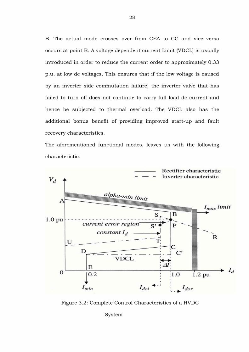
B. The actual mode crosses over from CEA to CC and vice versa

occurs at point B. A voltage dependent current Limit (VDCL) is usually

introduced in order to reduce the current order to approximately 0.33

p.u. at low dc voltages. This ensures that if the low voltage is caused

by an inverter side commutation failure, the inverter valve that has

failed to turn off does not continue to carry full load dc current and

hence be subjected to thermal overload. The VDCL also has the

additional bonus benefit of providing improved start-up and fault

recovery characteristics.

The aforementioned functional modes, leaves us with the following

characteristic.

Figure 3.2: Complete Control Characteristics of a HVDC

System

29

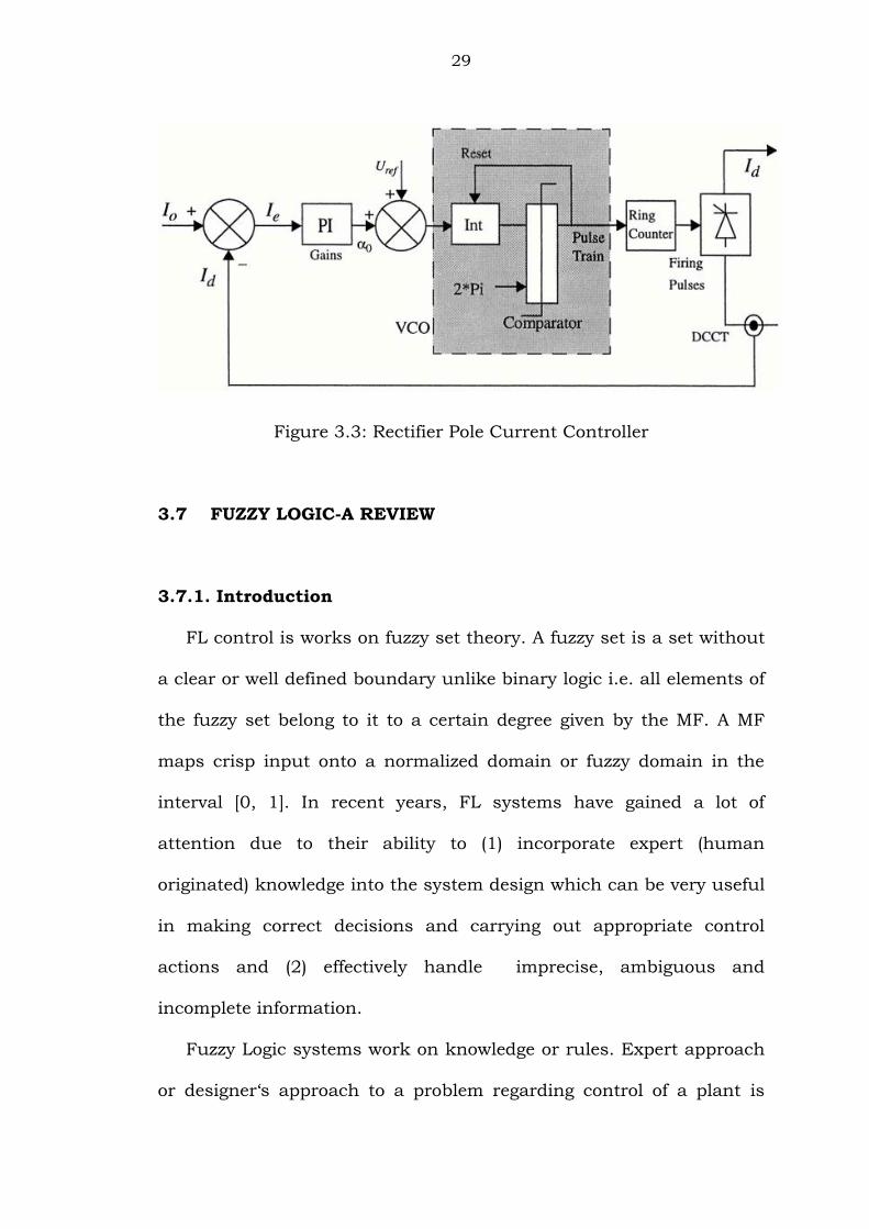
Figure 3.3: Rectifier Pole Current Controller

3.7 FUZZY LOGIC-A REVIEW

3.7.1. Introduction

FL control is works on fuzzy set theory. A fuzzy set is a set without

a clear or well defined boundary unlike binary logic i.e. all elements of

the fuzzy set belong to it to a certain degree given by the MF. A MF

maps crisp input onto a normalized domain or fuzzy domain in the

interval [0, 1]. In recent years, FL systems have gained a lot of

attention due to their ability to (1) incorporate expert (human

originated) knowledge into the system design which can be very useful

in making correct decisions and carrying out appropriate control

actions and (2) effectively handle imprecise, ambiguous and

incomplete information.

Fuzzy Logic systems work on knowledge or rules. Expert approach

or designer„s approach to a problem regarding control of a plant is

30

accumulated in the knowledge base as clear IF-THEN rules and this

knowledge base is used by Fuzzy Logic Controller to deduce

appropriate control action employing an inference strategy.

Overall, Fuzzy Logic controller acts as a buffer between a

nonlinear, highly complex system and desired control output, offering

numerous advantages such as providing a model free approach,

allowing human intelligence to be included in the control scheme and

ability to perform any nonlinear control action as fuzzy systems are

universal.

In recent years the fuzzy logic control technique has been used in

many applications, by which the controller performance can be

improved significantly as compared to conventional methods in the

presence of model uncertainties. In this chapter a basic introduction

about fuzzy logic design technique is given which describes the main

parts of the fuzzy controller and the description of each component is

given in detail.

3.7.2. Fuzzy Sets

As per the properties of classical set theory we speak whether an

element do or do not belong to a set. For eg: It‟ s 100% percent true

that the number three is a one among the set of odd numbers

and 100% percent false that it belongs to the set of even numbers.

But in the case of fuzzy an object partly will be a member of fuzzy set

and at the same instant to another set.

31

Let G be very big space all its components represented by y, then a

fuzzy set B in G is denoted as a set of prearranged pairs.

GyyxB B ),(,{ --------------------------------------(3.10)

B(y) is called the membership function (or MF) of y in B. MF‟S

relates all members of G to a value between 0 and 1. Degrees of

fuzziness are not similar to probability percentages, Probabilities tell

us whether a thing will happen or not, fuzziness defines the extent to

which something occurs.

3.7.3. Membership Function.

Membership functions can be a variety of shapes, the most

usual being triangular, trapezoidal, singleton or an exponential. The

simplest membership function is a straight line. A triangular

membership function is formed by a number of straight lines.

Trapezoidal, Gaussian, and bell-shaped functions are also extensively

used .In [31] it is concluded that the performance of fuzzy logic fault

detector designed considering three membership functions of

triangular shape is better than trapezoidal and Gaussian membership

functions. In [32] the investigation concluded that shape of MF‟s

slightly affect the performance with nonlinear MF‟s (Gaussian ) being

better than linear MF‟s. Polynomial distribution has a slightly worse or

similar performance to linear distribution. Therefore, linear

distribution of MF‟s is recommended to be used for the control of

HVDC systems. Investigations available in literature [33] and [34]

32

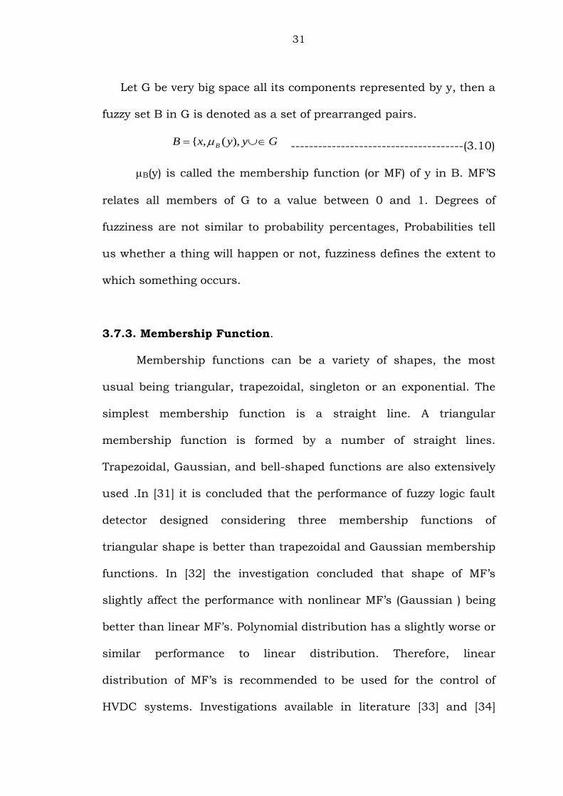
focused the extensive used of four basic membership functions. The

following Fig(3.4) is the representation of those basic membership

Functions usually employed.

Figure 3.4 (a) Trapezoidal (b) Triangular

(c ) Gaussian (d) Bell Shaped MF‟s

3.7.4. Fuzzy Rules

An example of an IF –THEN rule can be explained by considering

the compensation in power systems.

If we consider a power system network, at some points a drop in

the voltage is observed and at some points a raise in the voltage is

indicated as load on the system varies. Generally compensation device

is to be connected where ever the voltage decreases. The terms raise

and drop , are linguistics, which are used to define entire set of fuzzy

rules to determine location to place the compensation device.

Truly speaking, a single rule by itself won‟t solve the problem in an

efficient manner. A rule base comprising of two or more rules need to

33

be played-off one other. Each rule gives us a fuzzy set. All these

generated fuzzy sets are segregated in to one output set and the

obtained set has to be defuzzified.

3.7.5 FLC Structure

In the conventional control, the amount of control is determined

in relation to a number of data inputs using a set of equations to

express the entire control process. Expressing human experience in

the form of a mathematical formula is a very difficult task, if not an

impossible one. Fuzzy logic provides a simple tool to interpret this

experience into reality. Fuzzy logic controllers are rule-based

controllers. The structure of the FLC resembles that of a knowledge

based controller except that the FLC utilizes the principles of the fuzzy

set theory in its data representation and its logic. The basic

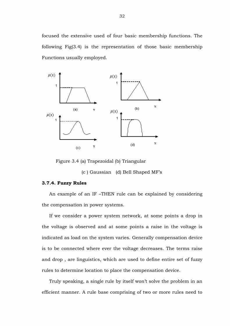
configuration of the FLC can be simply represented in four parts, as

shown in figure (3.5).Role played by the various parts is explained

briefly in the next few lines.

• Fuzzification module – the functions of which are first, to read,

measure, and scale the control variable (speed, acceleration) and,

second, to transform the measured numerical values to the

corresponding linguistic (fuzzy variables with appropriate

membership values);

• Knowledge base - this includes the definitions of the fuzzy

membership functions defined for each control variables and the

34

necessary rules that specify the control goals using linguistic

variables;

• Inference mechanism – it should be capable of simulating human

decision making and influencing the control actions based on fuzzy

logic;

• Defuzzufication module – which converts the inferred decision from

the linguistic variables backthe numerical values.

Figure 3.5 Basic Block Diagram of Fuzzy Logic Controller

3.7.6 FLC DESIGN

The design process of an FLC may split into various tasks which can

be described under various headings as follows:

35

a. Selection of the control variables

The selection of control variables (controlled inputs and outputs)

depends on the nature of the controlled system and the desired

output. Usually the output error (e) and the rate or derivative of the

output (de) are used as controller inputs. Some researchers have also

proposed the use of error and the integral of error as an input to the

FLC [33].

b. Representation of Membership functions

Each of the FLC input signal and output signal, fuzzy variables

(Xj={e, de,u}), has the real line R as the universe of discourse. In

practice, the universe of discourse is restricted to a comparatively

small interval [Xminj, Xmaxj]. The universe of discourse of each fuzzy

variables can be quantized into a number of overlapping fuzzy sets

(linguistic variables).The number of fuzzy sets for each fuzzy variables

varies according to the application. The reasonable number is an odd

number (3,5,7…). Increasing the number of fuzzy sets results in a

corresponding increase in the number of rules.

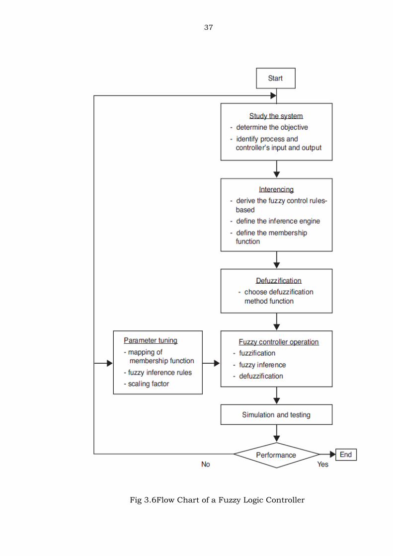
c. Defuzzification strategy

Defuzzification is a process of converting the FLC inferred control

actions from fuzzy vales to crisp values. This process depends on the

output fuzzy set, which is generated from the fired rules. The

performance of the FLC depends very much on the deffuzzification

36

process. This is because the overall performance of the system under

control is determined by the controlling signal (the defuzzified output

of the FLC.As mentioned in [33] various defuzzification methods have

been proposed to convert the output of the fuzzy controller to a crisp

value required by the plant. These methods are: Center of Area (COA),

Center of Sum (COS), Height Method (HM), Mean of maxima (MOM),

Center of Largest (COLA) and First maxima (FM).The flow chart

representing the various operations involved can be drawn as shown

in the figure (3.6).

The main part of the FLC is the Rule Base and the Inference

Mechanism. The rule base is normally expressed in a set of Fuzzy

Linguistic rules, with each rule triggered with varying belief for

support. The ith linguistic control rule can be expressed as:

Ri: If ei is Ai and dei is Bi THEN ui is Ci,

Where Ai and Bi (antecedent), Ci (consequent) are fuzzy variables

characterized by fuzzy membership functions.

37

Fig 3.6Flow Chart of a Fuzzy Logic Controller

38

3.8. ASPECTS OF NEURAL NETWORKS UTILISED IN THE THESIS

3.8.1. Introduction Artificial Neural networks are data handling prototypes comprising

networked data processing elements called neurons which work

together to perform a specific task. A data archetype is utilized to

teach NN . Constituents of the NN which handles information are

known as neurons. A neuron takes many inputs and gives an output.

The firing principle decides the output to be engendered for a specific

sample of input. Weight allocated to a particular node is a

consequence of effect of an input on the output. The neuron gives us

an output if the sum of the products of inputs and their

corresponding weights exceeds an upper limit.

In a feed Forward Neural Network the parameters traversal is form

input to output. On the contrary in feedback networks data takes the

path of various loops and can travel in any direction from input to

output or output to input.

3.8.2. Back Propagation Algorithm

The process involved in BPA can be demonstrated by considering a

three layer feed forward network consisting of a input, output as well

as a hidden layer.

39

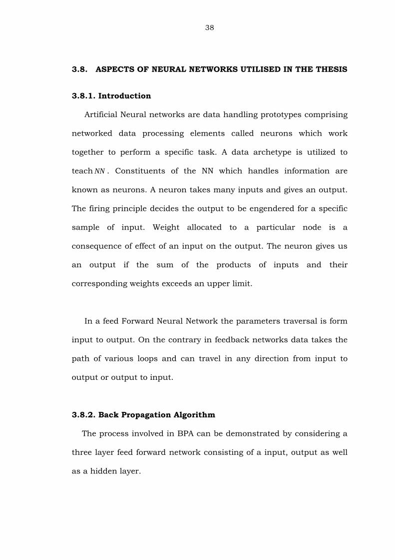
Figure 3.7 A Three Layer Neural Network

Figure 3.7 accepts 1x and 2x as inputs and delivers output

1Y .

Every neuron is linked with two factors. First parameter finds

summation of products of input and their corresponding weights. The

second quantity implements a nonlinear function, called Neural

Activation Function. The first parameter yields e , and )(efy is

output y of neuron.

40

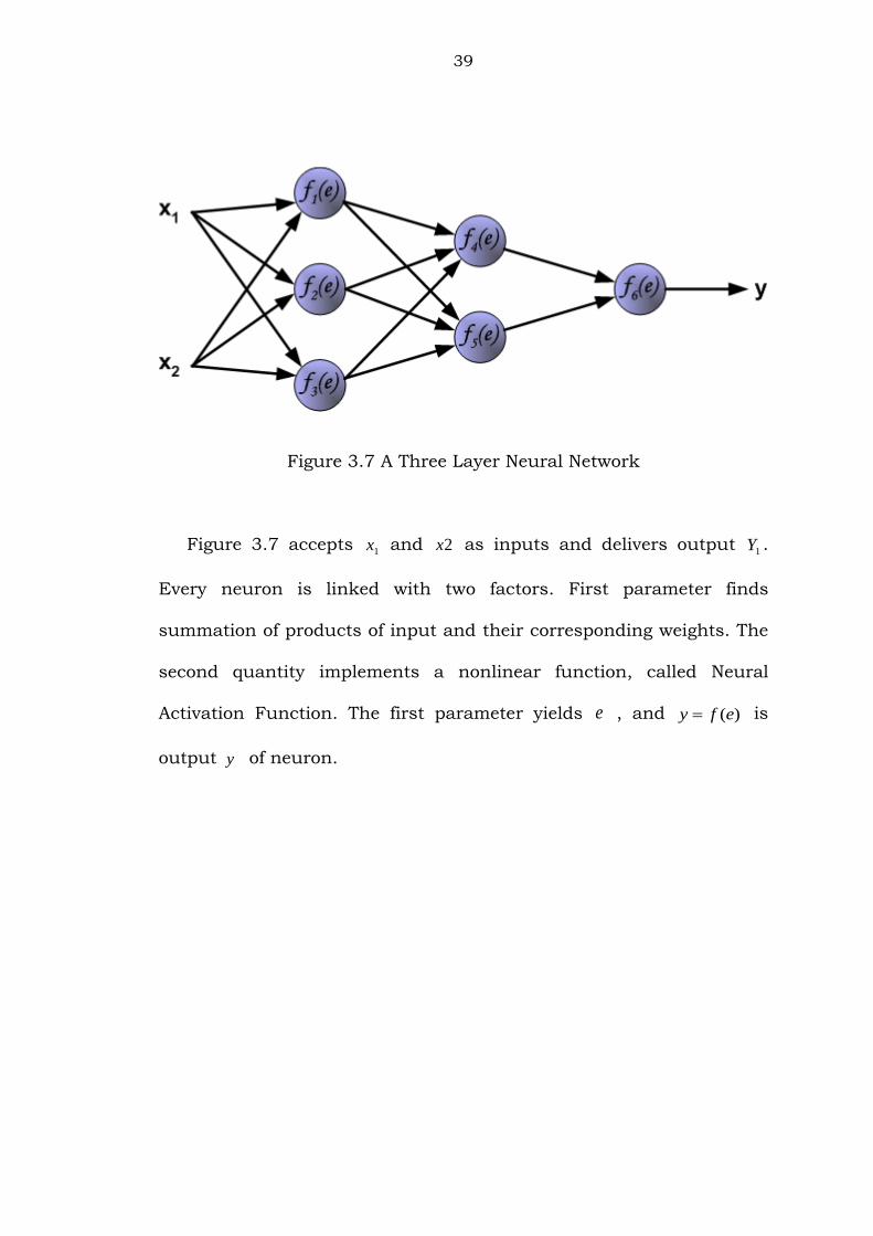
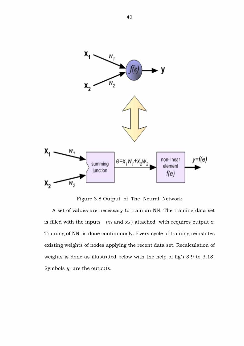
Figure 3.8 Output of The Neural Network

A set of values are necessary to train an NN. The training data set

is filled with the inputs (x1 and x2 ) attached with requires output z.

Training of NN is done continuously. Every cycle of training reinstates

existing weights of nodes applying the recent data set. Recalculation of

weights is done as illustrated below with the help of fig‟s 3.9 to 3.13.

Symbols yn are the outputs.

41

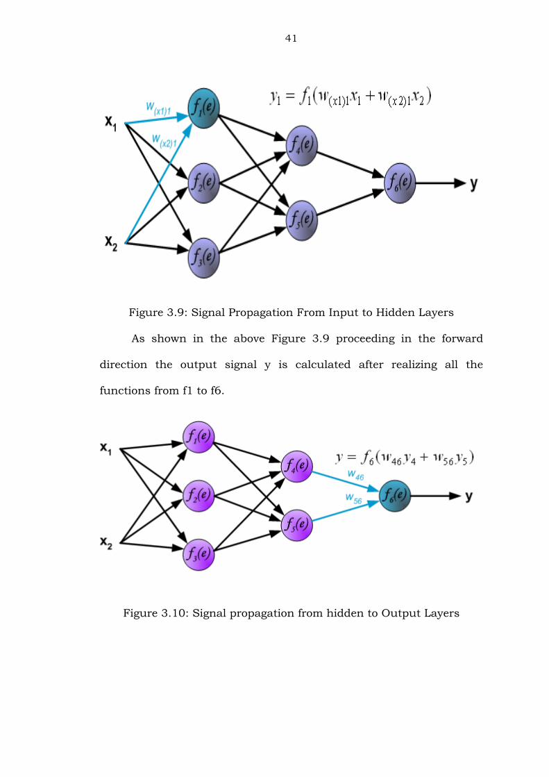
Figure 3.9: Signal Propagation From Input to Hidden Layers

As shown in the above Figure 3.9 proceeding in the forward

direction the output signal y is calculated after realizing all the

functions from f1 to f6.

Figure 3.10: Signal propagation from hidden to Output Layers

42

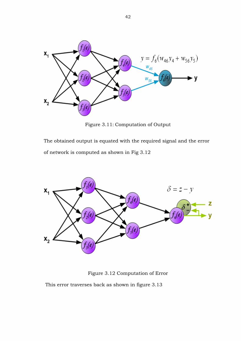
Figure 3.11: Computation of Output

The obtained output is equated with the required signal and the error

of network is computed as shown in Fig 3.12

Figure 3.12 Computation of Error

This error traverses back as shown in figure 3.13

43

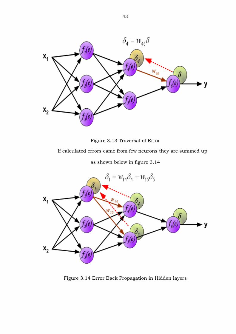
Figure 3.13 Traversal of Error

If calculated errors came from few neurons they are summed up

as shown below in figure 3.14

Figure 3.14 Error Back Propagation in Hidden layers

44

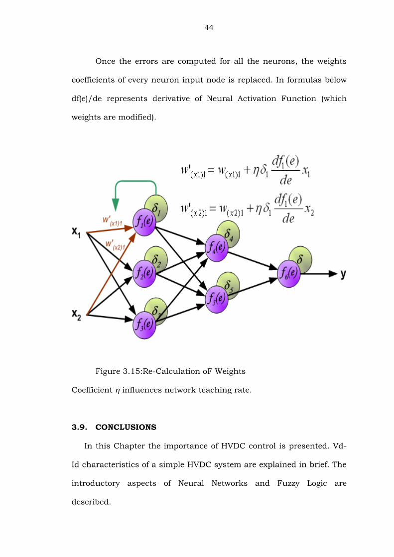
Once the errors are computed for all the neurons, the weights

coefficients of every neuron input node is replaced. In formulas below

df(e)/de represents derivative of Neural Activation Function (which

weights are modified).

Figure 3.15:Re-Calculation oF Weights

Coefficient η influences network teaching rate.

3.9. CONCLUSIONS

In this Chapter the importance of HVDC control is presented. Vd-

Id characteristics of a simple HVDC system are explained in brief. The

introductory aspects of Neural Networks and Fuzzy Logic are

described.