characterizing the behavior of magnetorheological …...characterizing the behavior of...
TRANSCRIPT

Characterizing the Behavior of Magnetorheological Fluids at High Velocities and High Shear Rates
by
Fernando D. Goncalves
Dissertation submitted to the Faculty of the
Virginia Polytechnic Institute and State University
in partial fulfillment of the requirements for the degree of
Doctor of Philosophy
in
Mechanical Engineering
Approved:
Dr. Mehdi Ahmadian Dr. Donald Baird
Dr. David Carlson Dr. Daniel Inman
Dr. Mary Kasarda Dr. Donald Leo
January 2005
Blacksburg, Virginia
Keywords: Magnetorheological, MR Fluid, MR Effect, Yield Stress, Bingham, Response Time, Dwell Time, Shear Rate, High Velocity
© 2005 Fernando D. Goncalves
Characterizing the Behavior of Magnetorheological Fluids at High Velocities and High Shear Rates
by
Fernando D. Goncalves
Abstract
Magnetorheological (MR) fluids offer solutions to many engineering challenges. The success of MR fluid is apparent in many disciplines, ranging from the automotive and civil engineering communities to the biomedical engineering community. This well documented success of MR fluids continues to motivate current and future applications of MR fluid.
One such application that has been considered recently is MR fluid devices for use in impact and other high velocity applications. In such applications, the fluid environment within the device may be well beyond the scope of our understanding for these fluids. To date, little has been done to explore the suitability of MR fluids in such high velocity and high shear applications.
While future applications may expose the fluid to adverse flow conditions, we must also consider current and existing applications which expose the fluid to extreme flow environments. Consider, for example, an MR damper intended for automotive primary suspensions, in which shear rates may exceed 105 s-1. Flow conditions within these dampers far exceed existing fluid behavior characterization.
The aim of the current study is to identify the behavior of the fluid under these extreme operating conditions. Specifically, this study intends to identify the behavior of MR fluid subject to high rates of shear and high flow velocities. A high shear rheometer is built which allows for the high velocity testing of MR fluids. The rheometer is capable of fluid velocities ranging from 1 m/s to 37 m/s, with corresponding shear rates ranging from 0.14x10⁵ s-1 to 2.5x10⁵ s-1. Fluid behavior is characterized in both the off-state and the on-state.
The off-state testing was conducted in order to identify the high shear viscosity of the fluid. Because the high shear behavior of MR fluid is largely governed by the behavior of the carrier fluid, the carrier fluid behavior was also identified at high shear. Experiments were conducted using the high shear rheometer and the MR fluid was shown to exhibit nearly Newtonian post-yield behavior. A slight thickening was observed for growing shear rates. This slight thickening can be attributed to the behavior of the carrier fluid, which exhibited considerable thickening at high shear.
The purpose of the on-state testing was to characterize the MR effect at high flow velocities. As such, the MR fluid was run through the rheometer at various flow velocities and a number of magnetic field strengths. The term “dwell time” is introduced and defined as the amount of time the fluid spends in the presence of a magnetic field. Two active valve lengths were considered, which when coupled to the fluid velocities,
iii
generated dwell times ranging from 12 ms to 0.18 ms. The yield stress was found from the experimental measurements and the results indicate that the magnitude of the yield stress is sensitive to fluid dwell time. As fluid dwell times decrease, the yield stress developed in the fluid decreases. The results from the on-state testing clearly demonstrate a need to consider fluid dwell times in high velocity applications. Should the dwell time fall below the response time of the fluid, the yield stress developed in the fluid may only achieve a fraction of the expected value. These results imply that high velocity applications may be subject to diminished controllability for falling dwell times.
Results from this study may serve to aid in the design of MR fluid devices intended for high velocity applications. Furthermore, the identified behavior may lead to further developments in MR fluid technology. In particular, the identified behavior may be used to develop or identify an MR fluid well suited for high velocity and high shear applications.

iv
“I can do all things through Christ who strengthens me.”
Philippians 4:13
v
Acknowledgements
I wish to thank my advisor Dr. Mehdi Ahmadian, who, over the course of my time at Virginia Tech, has been a great source of encouragement. Dr. Ahmadian has served as advisor and friend, and his support is truly appreciated. I also wish to thank the members of my Ph.D. committee for their guidance and support throughout this particular effort and, more generally, for their council during my time at Virginia Tech. Specifically, I would like to offer thanks to Dr. Daniel Inman, Dr. Donald Leo, Dr. Mary Kasarda, Dr. Donald Baird, and Dr. David Carlson. Special thanks are due to Dr. David Carlson, from Lord Corporation for agreeing to serve on my committee. Dr. Carlson has been a great resource and his involvement in my research is greatly appreciated. I would also like to thank Dr. Lynn Yanyo at Lord Corporation for her valuable feedback. Thanks are also due to Lord Corporation for their generous contribution to the Advanced Vehicle Dynamics Laboratory. For financial support during my time at Virginia Tech I am grateful to the Department of Mechanical Engineering.
I would also like to thank Dr. Baird in the Chemical Engineering Department for allowing the use of the equipment in the Polymer Processing Lab. Special thanks are due to his students, Matt Wilding and Chris Seay, for their assistance in making measurements on the fluid. This work has also been aided by the hard work of a number of individuals in the machine shop in the Department of Mechanical Engineering. Specifically, I would like to thank Billy Songer, James Dowdy, Timmy Kessinger, and Johnny Cox for their hard work and patience. Their guidance and effort has been a great contribution to this work and does not go unnoticed. I would also like to recognize the efforts of Bob Simonds in the Engineering Science and Mechanics Department. I am grateful to Mr. Simonds for helping me with all things related to MTS.
I would like to thank Dr. Jeong-Hoi Koo, colleague and great friend, for his constant support and encouragement. I am indebted to Jeong-Hoi for his valuable assistance on a countless number of occasions. I would also like to thank Dr. Nathan Siegel who provided valuable insight into my work for which I am truly grateful. I would also like to thank all the members of AVDL, past and present, for their companionship and memories. I also wish to list a group of friends whose companionship has meant a lot to me during my time at Virginia Tech. This list includes Jeong-Hoi Koo, Nathan Siegel, Michael Seigler, Emmanuel Blanchard, Mohammad Elahinia, and others. Thank you!
I would like to express my deepest gratitude to my parents, Manuel and Joana Goncalves, who’ve given more than I could ever hope to repay. For their love, support, and sacrifice I am forever grateful. To my brother Manny, I would like to express thanks for always looking after me. True to the big brother role, Manny has always been concerned with my well being, and for this I am grateful.
In words it would be difficult for me to express my gratitude to my fiancée, Courtney Mulligan. Her support, encouragement, and understand over the years is overwhelming. I look forward to expressing my gratitude in our coming future.
Finally, I would like to thank the Lord for being by my side always. I earn strength through my faith in God and his faith in me.

vi
Contents
Abstract_______________________________________________________________________________ ii Acknowledgements______________________________________________________________________ v List of Tables _________________________________________________________________________viii List of Figures__________________________________________________________________________ ix
1 INTRODUCTION _______________________________________________________________1
1.1 MOTIVATION______________________________________________________________1 1.2 OBJECTIVES_______________________________________________________________2 1.3 APPROACH _______________________________________________________________3 1.4 CONTRIBUTIONS ___________________________________________________________3 1.5 OUTLINE _________________________________________________________________4
2 MR FLUIDS AND DEVICES ______________________________________________________5
2.1 MAGNETORHEOLOGICAL FLUIDS_______________________________________________5 2.2 MR FLUID DEVICES _________________________________________________________6
2.2.1 MR devices in automotive applications _________________________________________8 2.2.2 MR devices in structural control applications ___________________________________10 2.2.3 Other MR fluid applications_________________________________________________12
2.3 MR FLUIDS IN HIGH VELOCITY APPLICATIONS____________________________________15 2.4 SUMMARY _______________________________________________________________17
3 MR FLUID MODELS ___________________________________________________________18
3.1 VISCO-PLASTIC MODELS ____________________________________________________18 3.2 QUASI-STEADY PARALLEL FLOW OF MR FLUID ___________________________________20
3.2.1 Velocity profile ___________________________________________________________21 3.2.2 Plug geometry____________________________________________________________22 3.2.3 Closed form solution for pressure gradient _____________________________________25
3.3 MODELING THE YIELD STRESS________________________________________________27 3.4 SUMMARY OF MR FLUID MODELS _____________________________________________30
4 EXPERIMENTAL APPROACH __________________________________________________31
4.1 DESIGN OF SLIT-FLOW RHEOMETER____________________________________________31 4.2 DATA ACQUISITION SYSTEM _________________________________________________37
4.2.1 Hardware components _____________________________________________________37 4.2.2 Software components ______________________________________________________40
4.3 EXPERIMENT PROCEDURES __________________________________________________42

vii
4.4 FRICTION FORCE __________________________________________________________44
5 OFF-STATE BEHAVIOR OF MR FLUID AT HIGH SHEAR RATES___________________46
5.1 MAGNETORHEOLOGICAL FLUID COMPOSITION ___________________________________46 5.2 FLUID PHYSICAL PROPERTIES ________________________________________________47
5.2.1 Carrier fluid properties ____________________________________________________48 5.2.2 MRF-132LD properties ____________________________________________________48
5.3 HIGH SHEAR BEHAVIOR _____________________________________________________50 5.3.1 Calculating the shear stress _________________________________________________50 5.3.2 High shear behavior of carrier fluid __________________________________________51 5.3.3 High shear behavior of MRF-132LD __________________________________________53
5.4 REYNOLDS NUMBER _______________________________________________________55 5.5 FLUID BEHAVIOR MODELS ___________________________________________________57
5.5.1 Proposed model for carrier fluid _____________________________________________58 5.5.2 Proposed model for MR fluid ________________________________________________60
5.6 TEMPERATURE CONSIDERATIONS _____________________________________________62 5.7 SUMMARY OF OFF-STATE BEHAVIOR ___________________________________________66
6 THE MR EFFECT AT HIGH VELOCITIES ________________________________________67
6.1 CREATING THE MR EFFECT __________________________________________________68 6.2 MR VALVE CONSIDERATIONS ________________________________________________70 6.3 FLUID DWELL TIME ________________________________________________________73 6.4 EXPERIMENTAL DETERMINATION OF THE YIELD STRESS ____________________________75 6.5 MAGNETIC FIELD TESTING___________________________________________________79 6.6 YIELD STRESS DEPENDENCE ON DWELL TIME ____________________________________83 6.7 MODELING THE MR EFFECT AT HIGH VELOCITIES _________________________________86 6.8 MR FLUID RESPONSE TIME __________________________________________________90 6.9 SUMMARY OF MR EFFECT AT HIGH VELOCITIES __________________________________92
7 CONCLUSIONS ________________________________________________________________94
7.1 RESEARCH SUMMARY ______________________________________________________94 7.2 RECOMMENDATIONS FOR FUTURE RESEARCH ____________________________________95
7.2.1 Non-steady conditions _____________________________________________________95 7.2.2 Evaluating different MR fluid compositions _____________________________________97 7.2.3 Other recommendations ____________________________________________________97
REFERENCES______________________________________________________________________98 VITA _____________________________________________________________________________103

viii
List of Tables
Table 5-1. Physical and chemical properties of carrier fluid (adapted from [67])........................................48 Table 5-2. Physical properties of MRF-132LD (adapted from [59])............................................................49 Table 5-3. Summary of fluid densities .........................................................................................................56 Table 5-4. Carrier fluid initial and final model parameters ..........................................................................59 Table 5-5. MR fluid initial and final model parameters ...............................................................................61 Table 5-6. Summary of proposed models.....................................................................................................66 Table 6-1. Summary of proposed MR effect models ...................................................................................89 Table 6-2. Summary of response time results ..............................................................................................91

ix
List of Figures
Figure 2-1. Activation of MR fluid: (a) no magnetic field applied; (b) magnetic field applied; (c) ferrous
particle chains have formed (© 2005 Lord Corporation [4]. All rights reserved).................................6 Figure 2-2. MR fluid modes: (a) valve mode; (b) shear mode; (c) squeeze mode (image adapted from [7]) 7 Figure 2-3. Section view of commercial MR fluid damper (image adapted from [8])...................................7 Figure 2-4. (a) Force-velocity illustration (image adapted from [9]); (b) experimentally obtained force-
velocity curve.........................................................................................................................................8 Figure 2-5. Base C5 Corvette and 50th anniversary Corvette with Magnetic Selective Ride Control
suspension (image adapted from [17])...................................................................................................9 Figure 2-6. Lord MotionMaster™ Ride Management System (© 2005 Lord Corporation [4]. All rights
reserved) ..............................................................................................................................................10 Figure 2-7. Schematic of Lord Corporation’s 180 kN seismic damper (© 2005 Lord Corporation [4]. All
rights reserved) ....................................................................................................................................11 Figure 2-8. Lord Corporation MR sponge damper (© 2005 Lord Corporation [4]. All rights reserved) ....12 Figure 2-9. Biedermann Motech prosthetic leg (© 2005 Lord Corporation [4]. All rights reserved) .........13 Figure 2-10. Lord Corporation MR rotary brake (© 2005 Lord Corporation [4]. All rights reserved) .......13 Figure 2-11. (a) QED Technologies' Q22 magnetorheological finishing machine; (b) diagram of polishing
process (images adapted from [37]).....................................................................................................14 Figure 3-1. Visco-plastic models often used to describe MR fluids.............................................................19 Figure 3-2. MR fluid flow through fixed parallel plates ..............................................................................20 Figure 3-3. Balance of forces on a fluid element in the plug region ............................................................23 Figure 3-4. Magnetic properties of MRF-132LD (© 2005 Lord Corporation [59]. All rights reserved): (a)
magnetic induction curves; (b) yield stress as a function of applied field ...........................................28 Figure 3-5. Predicted yield stress as a function of applied field...................................................................29 Figure 4-1. Venturi schematic ......................................................................................................................32 Figure 4-2. (a) MR rheometer mounted in MTS load frame; (b) Close-up of MR rheometer......................32 Figure 4-3. Main tube...................................................................................................................................33 Figure 4-4. Piston with Viton® o-ring and nylon bushing ............................................................................34 Figure 4-5. Reducer - used to reduce diameter from 101.6 mm to 10 mm...................................................35 Figure 4-6. 1x10 mm flow channel and MR valve.......................................................................................36 Figure 4-7. Electromagnet used to activate MR fluid...................................................................................37 Figure 4-8. Gauss-meter and "ultra-thin" transverse probe ..........................................................................38 Figure 4-9. Fluid temperature measurements: (a) thermocouple probe mounted at exit of rheometer; (b)
Fluke-52 and digital filters used to monitor fluid temperature ............................................................39 Figure 4-10. Circuit box and power supplies used to power the electromagnet ...........................................39 Figure 4-11. Data acquisition and control block diagram ............................................................................40
x
Figure 4-12. dSPACE ControlDesk used to monitor various signals and to control the electromagnet.......41 Figure 4-13. MTS TestWare SX software used to control hydraulic actuator .............................................42 Figure 4-14. Ramp input used in steady flow experiments ..........................................................................43 Figure 4-15. Friction model of rheometer ....................................................................................................45 Figure 5-1. SEM image of carbonyl iron powder (image adapted from [66])..............................................47 Figure 5-2. Shear thinning behavior of MRF-132LD (© 2005 Lord Corporation [59]. All rights reserved)
.............................................................................................................................................................50 Figure 5-3. Force versus position for carrier fluid........................................................................................52 Figure 5-4. Carrier fluid high shear behavior: (a) shear stress versus shear rate; (b) apparent viscosity
versus shear rate (collected at an average initial fluid temperature of 24.4 °C)...................................53 Figure 5-5. Force versus position for MR fluid............................................................................................54 Figure 5-6. MR fluid high shear behavior: (a) shear stress versus shear rate; (b) apparent viscosity versus
shear rate (collected at an average initial fluid temperature of 25.8 °C)..............................................55 Figure 5-7. Reynolds number for carrier fluid and MR fluid .......................................................................57 Figure 5-8. Flow chart for optimization routine ...........................................................................................58 Figure 5-9. Carrier fluid model results: (a) Proposed model and experimental data; (b) model error..........60 Figure 5-10. MR fluid model results: (a) Proposed model and experimental data; (b) model error.............62 Figure 5-11. Carrier fluid temperature response: (a) fluid exit temperature over piston stroke; (b) fluid
initial temperature and final temperature as a function of piston velocity ...........................................64 Figure 5-12. MR fluid temperature response: (a) fluid exit temperature over piston stroke; (b) fluid initial
temperature and final temperature as a function of piston velocity .....................................................65 Figure 6-1. Field dependent yield stress for MRF-132LD (© 2005 Lord Corporation [59]. All rights
reserved) ..............................................................................................................................................68 Figure 6-2. Electromagnet-controlled MR valve (© 2005 Lord Corporation [70]. All rights reserved) .....69 Figure 6-3. Section view of commercial MR fluid damper (image adapted from [8]).................................69 Figure 6-4. Axisymmetric MR valves: (a) single-stage piston (image adapted from [70]); (b) dual-stage
piston (image adapted from [73]); (c) 3-stage piston (© 2005 Lord Corporation [4]. All rights
reserved) ..............................................................................................................................................72 Figure 6-5. MR valve flow schematic illustrating fluid response to a magnetic field ..................................74 Figure 6-6. Dwell time of fluid through active valve length ........................................................................75 Figure 6-7. Flow channel showing MR active valve portion .......................................................................76 Figure 6-8. Flow transition through fixed parallel plates .............................................................................77 Figure 6-9. Force versus position: (a) 25.4 mm valve at 100 kA/m; (b) 25.4 mm valve at 200 kA/m; (c)
6.35 mm valve at 100 kA/m; (d) 6.35 mm valve at 200 kA/m ............................................................80 Figure 6-10. Pressure in flow channel as a function of fluid velocity: (a) 25.4 mm valve; (b) 6.35 mm valve
.............................................................................................................................................................81 Figure 6-11. Yield stress as a function of fluid velocity: (a) 25.4 mm MR valve; (b) 6.35 mm MR valve.83

xi
Figure 6-12. Yield stress as a function of dwell time: (a) 25.4 mm MR valve; (b) 6.35 mm MR valve ......84 Figure 6-13. Normalized yield stress as a function of dwell time: (a) 25.4 mm MR valve; (b) 6.35 mm MR
valve.....................................................................................................................................................86 Figure 6-14. Normalized yield stress as a function of dwell time: (a) 100 kA/m; (b) 200 kA/m.................88 Figure 6-15. Proposed MR effect model comparison: (a) 100 kA/m; (b) 200 kA/m....................................90 Figure 6-16. Identifying the response time of MR fluid at 100 kA/m and 200 kA/m ..................................92 Figure 7-1. Plug decomposition under non-steady flow...............................................................................96
1
1 Introduction
The purpose of this chapter is to express the motivation for this work and to introduce the
objectives. With the objectives identified, the means by which the objectives will be met
are discussed. Finally, a discussion of the contributions of this work and an outline of
this document conclude the chapter.
1.1 Motivation
Magnetorheological (MR) fluids offer solutions to many engineering challenges. The
success of MR fluid is apparent in many disciplines, ranging from the automotive and
civil engineering communities to the biomedical engineering community. There have
been a countless number of studies which identify the benefits of using MR devices in
these and other fields. This well documented success of MR fluids continues to motivate
current and future applications of MR fluid.
Much of the success of MR fluid devices is largely due to advancements in fluid
technology. Today’s MR fluids are capable of achieving yield stresses in excess of 80
kPa which indicates an impressive range of fluid controllability and dynamic range. The
fluids have also exhibited improved stability behavior. Moreover, the durability and life
of the fluid have developed such that the fluid can be considered for commercial
implementation. The performance of today’s MR fluids is the result of a great number of
studies which identify the properties and behavior of MR fluids. The literature is well
populated with works related to the behavior of MR fluid or the performance of specific
MR fluid devices. In many cases, knowledge of the performance of the MR device
precedes a thorough understanding of the behavior of the fluid operating in such a device.
This is the case for many MR fluid devices. An MR device intended for one application
often finds use in an alternate application in which the operating conditions of the fluid
differ greatly from the original application. An example of this “borrowed” technology is
the many applications of Lord Corporation’s MotionMaster™ damper. This damper,
originally intended for seat suspensions in trucks and buses, has also been considered for
service in civil engineering applications and in prosthetic limbs. In each of these
applications, the operating conditions of the fluid vary considerably. Perhaps a more

2
extreme example would be the use of MR automotive dampers (intended for vehicle
primary suspensions) in impact or shock loading applications. Here again, the conditions
inside the damper vary considerably.
While fluid behavior may be well understood under certain operating conditions,
there is a great need to understand fluid behavior in all regimes of operation. Fluid
behavior is often characterized in a laboratory in which fluid conditions are moderate, at
best, and are not representative of the conditions within many existing MR fluid devices.
In many current applications of MR fluids, fluid conditions within the device are far
beyond any published behavior characterization. In order to support existing
applications, and encourage emerging applications, there is a need to identify MR fluid
behavior under conditions that are representative of those observed in current and future
devices. Specifically, there is a need to understand the behavior of MR fluids at high
shear rates and high flow velocities.
1.2 Objectives
This research intends to address the lack of awareness regarding MR fluid behavior under
adverse flow conditions. The hope here is to provide a thorough investigation of the
behavior of MR fluid operating in conditions that are in the range of those observed in
current devices.
The primary objectives of this research can be summarized as follows:
1. Better understand the rheological behavior of MR fluids at high shear rates and
high velocities
2. Improve existing models for MR fluids such that they can accurately represent the
fluid behavior at high shear rates
3. Verify, to the extent possible, the accuracy of the proposed models through
comparison with experimental results
4. Potentially provide engineering guides that can be used for designing MR fluids
for high shear rate applications

3
1.3 Approach
With the primary objective of this work identified as characterizing the behavior of MR
fluids at high shear rates and high velocities, a means for testing the fluid under such
conditions was necessary. To this end, a slit-flow rheometer was designed and built
which allowed for the high velocity testing of MR fluid. Similar to a conventional
capillary rheometer, the slit-flow rheometer is capable of generating fluid velocities many
times greater than the piston velocity. A series of experiments were conducted with the
fluid in an unenergized state and at various magnetic field strengths. Results of these
experiments are used to identify fluid behavior at high shear rates and high flow
velocities. Specifically, for the zero-field tests, the fluid viscosity is found at high rates
of shear. For the magnetic field testing, the yield stress developed in the fluid is found to
quantify the MR effect at high flow velocities.
The behavior observed in the experiments is compared to the behavior predicted
by existing models. Departures between the model and the experiment are identified.
Improvements to existing models are proposed which account for the behavior observed
at high velocities.
1.4 Contributions
This research has identified the behavior of MR fluid in, as yet, uncharacterized flow
conditions. The high shear behavior of the fluid was identified in both the off-state and
the on-state. Under such conditions, the behavior of the fluid has been shown to depart
from commonly accepted behavior of the fluid. The current study may serve as a
platform for future studies in the high velocity behavior of MR fluid, and has identified
practical considerations for MR devices intended for high velocity and high shear
applications.
Specific contributions can be summarized as follows:
• The off-state behavior of the MR fluid has been identified at shear rates as high as
2.5x10⁵ s-1. Fluid viscosity was identified at these shear rates.
• The behavior of the carrier fluid has been identified at high shear.

4
• The high velocity behavior of MR fluid in the on-state was evaluated. The MR
effect was characterized as a function of fluid dwell time.
• Practical limitations of MR fluids at high velocities have been identified. High
velocity applications of MR fluids may be subject to diminished controllability
for falling dwell times.
• The outcome of the current study may serve as a foundation for future studies in
the high shear and high velocity applications of MR fluid and MR fluid devices.
1.5 Outline
The next chapter, Chapter 2, provides background on MR fluids and MR fluid devices. A
general discussion of the fundamental behavior of MR fluids is presented. Chapter 2 also
discusses a number of MR fluid devices and their applications. The chapter concludes
with an introduction of emerging applications of MR fluids and reiterates the motivation
for this work. Chapter 3 reviews common visco-plastic models, often used to describe
the field dependent yield stress of MR fluids. A model of quasi-steady parallel flow of
MR fluid is developed. Chapter 3 also discusses a model which is used to predict the
yield stress for any MR fluid as a function of magnetic field strength. In Chapter 4, the
high shear rheometer used in this study is discussed in detail. Furthermore, the
experimental approach is introduced. Results for the high shear behavior of the
unenergized fluid are presented in Chapter 5. This chapter discusses, in detail, the
composition and properties of the MR fluid used in this study. The high shear viscosity
is found from experimental measurements. In Chapter 6, the high flow velocity behavior
is discussed. In Chapter 6, the MR effect is introduced and experimental results for the
fluid under various magnetic field strengths are presented. Chapter 6 also provides a
discussion on proposed improvements to existing models. Finally, Chapter 7 provides a
summary of the work and highlights the significant results. Recommendations for future
work are also presented in Chapter 7.
5
2 MR Fluids and Devices
Magnetorheological (MR) fluids belong to a class of fluids that exhibit variable yield
stress. Discovered by Jacob Rabinow at the US National Bureau of Standards in 1948
[1], MR fluid has the ability to change from a fluid state to a semi-solid or plastic state
instantaneously upon the application of a magnetic field. In this semi-solid state, the
fluid exhibits viscoplastic behavior that is characterized by the field-dependent yield
stress. It is this field-dependent yield stress, and their fast response time, that make MR
fluids an attractive technology for many applications.
MR fluid’s success has been apparent in many fields of engineering and new
applications continue to emerge. While much of the fluid’s success has been realized in
devices intended for automotive or civil engineering applications, recent studies have
investigated the fluid’s promise in impact or shock related applications. These emerging
applications, and many current applications, subject the fluid to extreme flow conditions.
Specifically, these flow environments or conditions include high shear and high velocity
flow. The challenge in such devices becomes the lack of information regarding the
behavior of MR fluid under these adverse operating conditions.
This chapter will review the fundamental behavior of MR fluids and present some
of the existing MR fluid devices. An introduction of some of the emerging applications
of MR fluids then follows. The chapter concludes with a discussion of some of the
challenges associated with the current and future use of MR fluids in, as yet,
uncharacterized flow conditions.
2.1 Magnetorheological fluids
In the absence of a magnetic field, MR fluid is free flowing with a consistency similar to
motor oil. The value of these fluids is realized when a magnetic field is applied; micron-
sized ferrous particles suspended in the fluid align parallel to the flux path, creating
particle chains. Figure 2-1 illustrates this process. Initially, the ferrous particles are in an
amorphous state as shown in Figure 2-1a. When a magnetic field is applied, the ferrous
particles begin to align along the flux path as shown in Figure 2-1b. Figure 2-1c shows

6
the ferrous particles aligned along the flux path creating particle chains in the fluid.
These particle chains resist and restrict fluid movement. As a result, a yield stress is
developed in the fluid. The degree of change is related to the magnetic field strength and
may occur in a matter of milliseconds [2, 3].
(a) (b) (c)(a) (b) (c)
Figure 2-1. Activation of MR fluid: (a) no magnetic field applied; (b) magnetic field applied; (c)
ferrous particle chains have formed (© 2005 Lord Corporation [4]. All rights reserved)
2.2 MR fluid devices
The benefit of the controllable yield stress in MR fluids has been realized in many
devices for various applications. The range of applications is impressive and indicates
the potential for future developments. In many such applications the fluid is employed in
one of three common modes (valve mode, shear mode, or squeeze mode). The three
modes are shown in Figure 2-2. Both valve and shear mode are commonly used in MR
dampers. Other applications of shear mode appear in MR brakes and clutches. In valve
mode, the fluid flows between fixed parallel plates. This pressure driven flow is
commonly referred to as Poiseuille flow. In shear mode, the fluid flows between parallel
plates sliding relative to each other with speed vo. This type of flow combines Poiseuille
flow with shear flow or Couette flow. Squeeze mode, less common than the other two
modes, has been considered for small amplitude vibration mitigation [5, 6]. In squeeze
mode, it is often assumed that the lateral flow of the fluid has Poiseuille-like behavior.

7
(a) (b) (c)(a) (b) (c)
Figure 2-2. MR fluid modes: (a) valve mode; (b) shear mode; (c) squeeze mode (image adapted from
[7])
The benefit of the controllable yield stress in MR fluids is often realized in
devices such as MR dampers. In both the automotive industry and the civil engineering
community, applications of MR dampers have been actively studied because of their
ability to respond quickly while providing large dynamic forces. Consider the section
view of an MR damper shown in Figure 2-3. Unlike hydraulic dampers, MR dampers do
not require mechanical valves to restrict flow. Instead, an electromagnetic coil is
incorporated into the piston and the reservoir is filled with MR fluid. With the
application of current through the wire leads, a magnetic field is developed in the annular
orifice. This magnetic field causes a yield stress to develop in the fluid as it passes the
through the flux path, thus increasing the apparent viscosity of the fluid. Because of their
ability to offer controllable damping force with minimal power requirements, MR fluid
dampers are considered semi-active damping elements. It is in this form that they have
served as solutions to many engineering challenges.
Figure 2-3. Section view of commercial MR fluid damper (image adapted from [8])
8
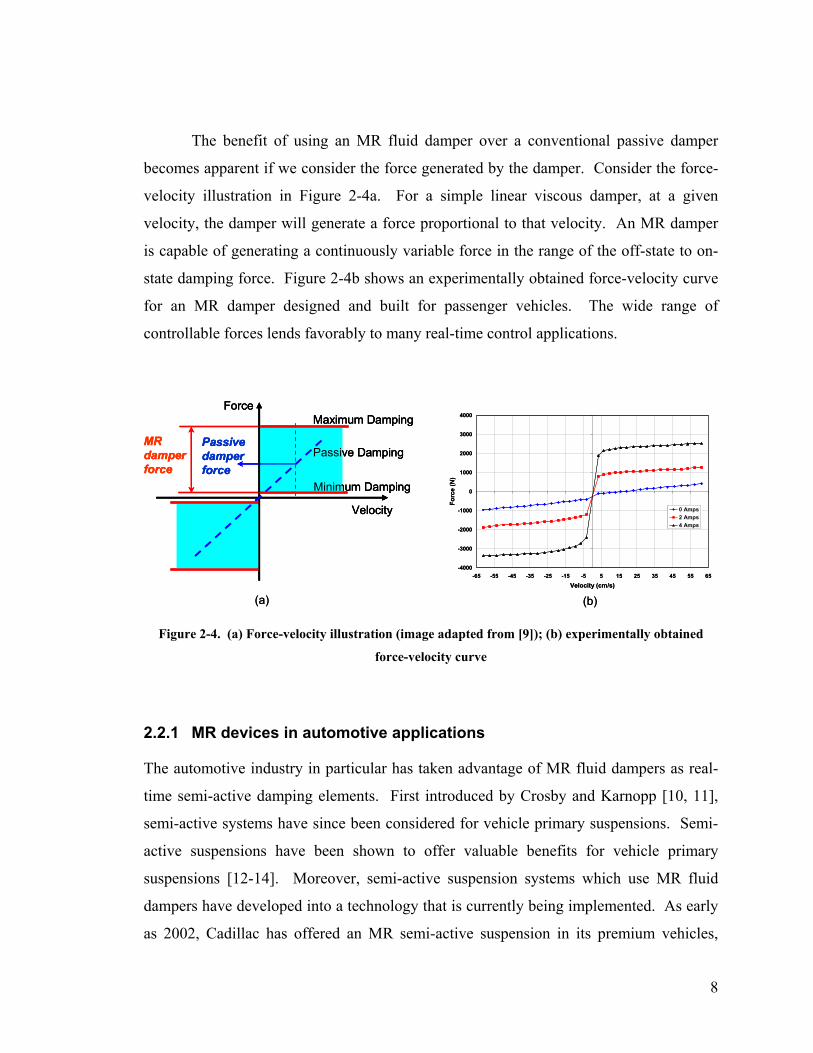
The benefit of using an MR fluid damper over a conventional passive damper
becomes apparent if we consider the force generated by the damper. Consider the force-
velocity illustration in Figure 2-4a. For a simple linear viscous damper, at a given
velocity, the damper will generate a force proportional to that velocity. An MR damper
is capable of generating a continuously variable force in the range of the off-state to on-
state damping force. Figure 2-4b shows an experimentally obtained force-velocity curve
for an MR damper designed and built for passenger vehicles. The wide range of
controllable forces lends favorably to many real-time control applications.
(a) (b)
-4000
-3000
-2000
-1000
0
1000
2000
3000
4000
-65 -55 -45 -35 -25 -15 -5 5 15 25 35 45 55 65
Velocity (cm/s)
Forc
e (N
)
0 Amps2 Amps4 Amps
Force
Velocity
Passive Damping
Maximum Damping
Minimum Damping
Passive damper force
MR damper force
(a) (b)
-4000
-3000
-2000
-1000
0
1000
2000
3000
4000
-65 -55 -45 -35 -25 -15 -5 5 15 25 35 45 55 65
Velocity (cm/s)
Forc
e (N
)
0 Amps2 Amps4 Amps
Force
Velocity
Passive Damping
Maximum Damping
Minimum Damping
Passive damper force
MR damper force
Force
Velocity
Passive Damping
Maximum Damping
Minimum Damping
Passive damper force
MR damper force
Figure 2-4. (a) Force-velocity illustration (image adapted from [9]); (b) experimentally obtained
force-velocity curve
2.2.1 MR devices in automotive applications
The automotive industry in particular has taken advantage of MR fluid dampers as real-
time semi-active damping elements. First introduced by Crosby and Karnopp [10, 11],
semi-active systems have since been considered for vehicle primary suspensions. Semi-
active suspensions have been shown to offer valuable benefits for vehicle primary
suspensions [12-14]. Moreover, semi-active suspension systems which use MR fluid
dampers have developed into a technology that is currently being implemented. As early
as 2002, Cadillac has offered an MR semi-active suspension in its premium vehicles,
9
such as the Seville STS and Escalade EXT [15, 16]. Currently, Cadillac offers a
Magnetic Ride Control suspension on the 2004 STS and the 2004 SRX. Other GM
brands are offering similar advanced suspensions. With the release of the 50th
anniversary Corvette, Chevrolet offered a Magnetic Selective Ride Control system. The
same suspension has carried over into the sixth generation Corvette. Advantages of this
suspension include real-time control and the ability of the suspension to adapt to
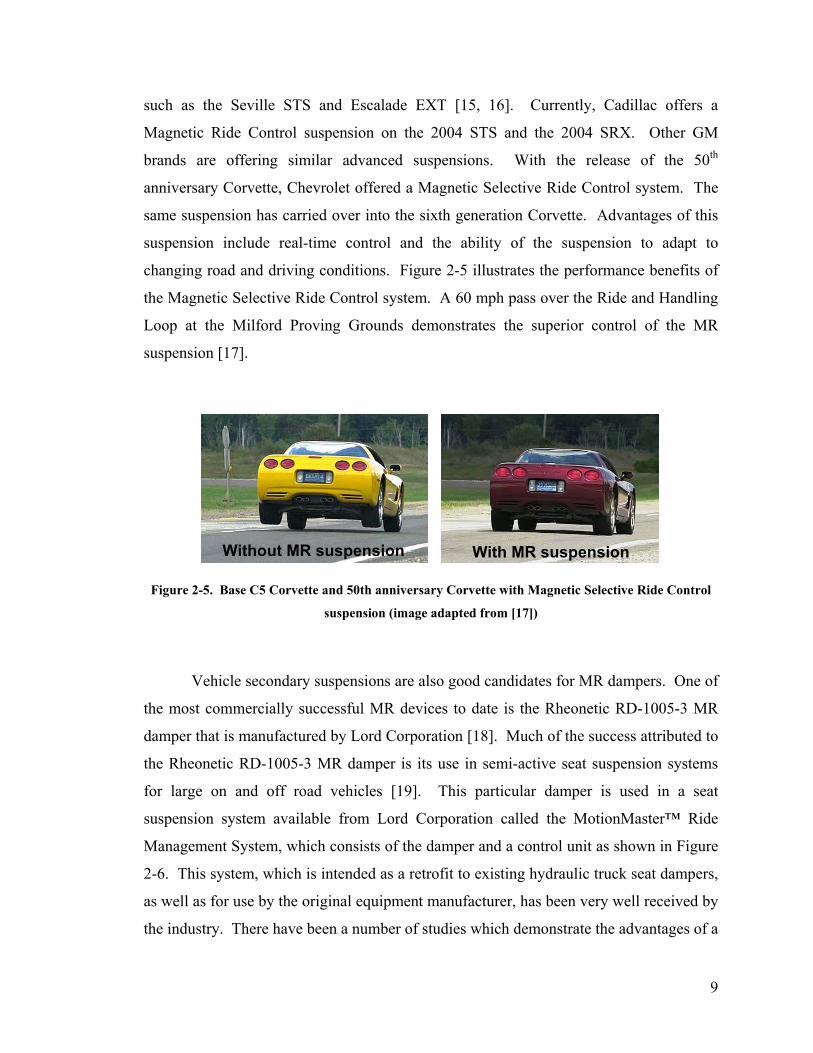
changing road and driving conditions. Figure 2-5 illustrates the performance benefits of
the Magnetic Selective Ride Control system. A 60 mph pass over the Ride and Handling
Loop at the Milford Proving Grounds demonstrates the superior control of the MR
suspension [17].
Without MR suspension With MR suspensionWithout MR suspension With MR suspension
Figure 2-5. Base C5 Corvette and 50th anniversary Corvette with Magnetic Selective Ride Control
suspension (image adapted from [17])
Vehicle secondary suspensions are also good candidates for MR dampers. One of
the most commercially successful MR devices to date is the Rheonetic RD-1005-3 MR
damper that is manufactured by Lord Corporation [18]. Much of the success attributed to
the Rheonetic RD-1005-3 MR damper is its use in semi-active seat suspension systems
for large on and off road vehicles [19]. This particular damper is used in a seat
suspension system available from Lord Corporation called the MotionMaster™ Ride
Management System, which consists of the damper and a control unit as shown in Figure
2-6. This system, which is intended as a retrofit to existing hydraulic truck seat dampers,
as well as for use by the original equipment manufacturer, has been very well received by
the industry. There have been a number of studies which demonstrate the advantages of a

10
semi-active damper over conventional passive dampers in secondary or seat suspensions
[20-23]. Agricultural off-highway vehicles also stand to benefit from the superior
vibration isolation available with the MotionMaster™ system. Sears Seating has
partnered with Lord Corporation to develop a MotionMaster™ system tailored for
agricultural and off-highway equipment [24]. School transportation officials have also
taken advantage of the MotionMaster™ system. In fact, in an effort to reduce worker
compensation claims, school transportation officials in many states have adopted the
MotionMaster™ Ride Management System for use in buses. When retrofitted with the
MotionMaster™ Ride Management System drivers report less fatigue and reduced back
and leg discomfort [25].
Figure 2-6. Lord MotionMaster™ Ride Management System (© 2005 Lord Corporation [4]. All
rights reserved)
2.2.2 MR devices in structural control applications
MR dampers have also gained considerable attention in structural control applications.
Seismic response reduction using MR dampers is an area of research that has received
considerable attention recently [26, 27]. Recently, large-scale MR fluid dampers have
been considered for structural vibration mitigation. A full-scale MR fluid damper has
been designed and built in order to test the suitability of such devices in civil engineering
applications [28, 29]. The double-ended design, shown in Figure 2-7, eliminates the need
for an accumulator to compensate for piston rod volume. Designed for a maximum force
of 200,000 N, the damper is approximately 1 m long with a mass of 250 kg.

11
Figure 2-7. Schematic of Lord Corporation’s 180 kN seismic damper (© 2005 Lord Corporation [4].
All rights reserved)
Other structures that have benefited from MR damper technology are cable-stayed
bridges. The Dongting Bridge is a cable-stayed bridge which crosses Dongting Lake
where it meets the Yangtze River in south central China. In June of 2002 the Dongting
Bridge became the first cable-stayed bridge to use MR dampers to suppress wind and rain
induced vibrations [30-32]. Results indicate significant vibration control effectiveness in
the cables that were damped with MR dampers.
MR dampers have also been considered for use in structural tuned vibration
absorbers. In such an application, the damper must be able to provide sufficient damping
force while still maintaining a low off-state force. The MR sponge damper, shown in
Figure 2-8, was a worthy candidate. Koo [9] showed that an MR sponge damper coupled
to a tuned vibration absorber (TVA) can provide benefits for controlling unwanted
vibrations in structures. The inherent difficulty with TVAs in structures is the inevitable
off-tuning of the TVA due to changes in the system’s operating conditions, i.e., mass or
stiffness changes over time. This off-tuning can lead to degradation in the performance
of the TVA. Koo showed that with the addition of an MR damper, the sensitivity of the
TVA system to changes in system operating conditions is reduced. In other words, the

12
MR TVA is more robust to changes in mass or stiffness. Because of its low off-state
damping, the MR sponge damper was a good candidate for such an application.
Figure 2-8. Lord Corporation MR sponge damper (© 2005 Lord Corporation [4]. All rights
reserved)
The MR sponge damper contains MR fluid in an absorbent matrix such as sponge,
open-celled foam, or fabric. The sponge keeps the MR fluid located in the active region
of the device where the magnetic field is applied. The device is operated in a direct shear
mode with a minimum volume of MR fluid (~3 mL). Moreover, the MR sponge device
does not require high-cost components, such as seals, rod surface finish, and the precision
mechanical tolerances that are normally associated with conventional fluid-filled MR
devices. Cost sensitive applications, such as domestic washing machines, stand to benefit
from the MR sponge damper [33]. Figure 2-8 shows the internal components of the MR
sponge damper. This MR sponge device is appropriate for many applications in which
low off-state damping is desired while still maintaining controllability in the on-state
force.
2.2.3 Other MR fluid applications
A rather innovative application of the Lord MotionMaster™ damper is its use in a
prosthetic leg that is being developed by Biedermann Motech GmbH [34]. The device,
shown in Figure 2-9, dramatically improves the mobility of leg amputees by mimicking a
natural gait. Coupled with a combination of sensors and controllers, the device can adapt
13
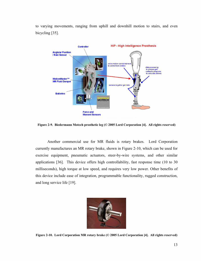
to varying movements, ranging from uphill and downhill motion to stairs, and even
bicycling [35].
Figure 2-9. Biedermann Motech prosthetic leg (© 2005 Lord Corporation [4]. All rights reserved)
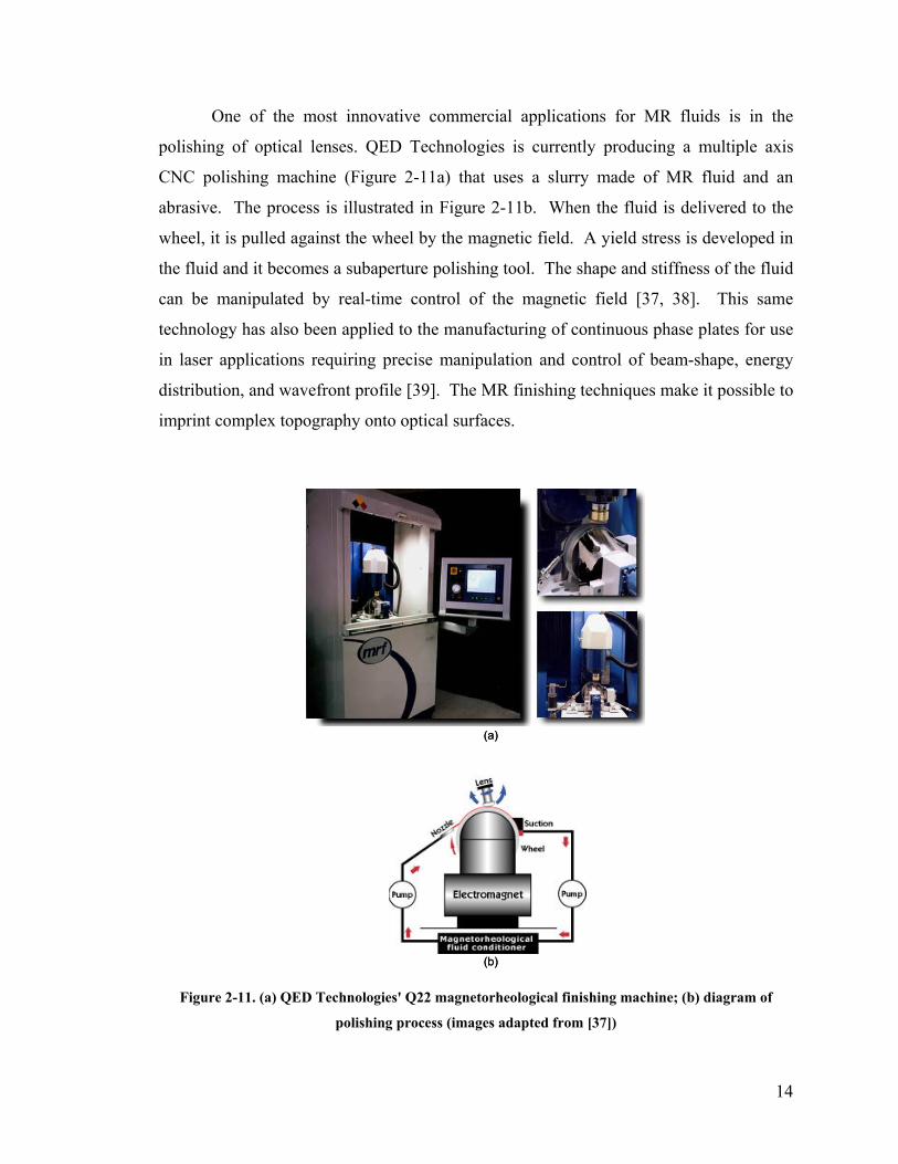
Another commercial use for MR fluids is rotary brakes. Lord Corporation
currently manufactures an MR rotary brake, shown in Figure 2-10, which can be used for
exercise equipment, pneumatic actuators, steer-by-wire systems, and other similar
applications [36]. This device offers high controllability, fast response time (10 to 30
milliseconds), high torque at low speed, and requires very low power. Other benefits of
this device include ease of integration, programmable functionality, rugged construction,
and long service life [19].
Figure 2-10. Lord Corporation MR rotary brake (© 2005 Lord Corporation [4]. All rights reserved)
14
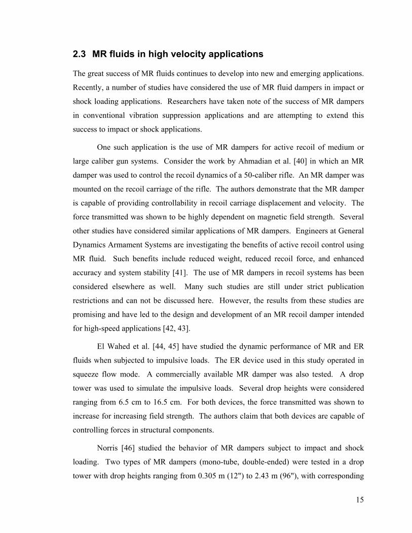
One of the most innovative commercial applications for MR fluids is in the
polishing of optical lenses. QED Technologies is currently producing a multiple axis
CNC polishing machine (Figure 2-11a) that uses a slurry made of MR fluid and an
abrasive. The process is illustrated in Figure 2-11b. When the fluid is delivered to the
wheel, it is pulled against the wheel by the magnetic field. A yield stress is developed in
the fluid and it becomes a subaperture polishing tool. The shape and stiffness of the fluid
can be manipulated by real-time control of the magnetic field [37, 38]. This same
technology has also been applied to the manufacturing of continuous phase plates for use
in laser applications requiring precise manipulation and control of beam-shape, energy
distribution, and wavefront profile [39]. The MR finishing techniques make it possible to
imprint complex topography onto optical surfaces.
(a)
(b)
(a)
(b)
Figure 2-11. (a) QED Technologies' Q22 magnetorheological finishing machine; (b) diagram of
polishing process (images adapted from [37])
15
2.3 MR fluids in high velocity applications
The great success of MR fluids continues to develop into new and emerging applications.
Recently, a number of studies have considered the use of MR fluid dampers in impact or
shock loading applications. Researchers have taken note of the success of MR dampers
in conventional vibration suppression applications and are attempting to extend this
success to impact or shock applications.
One such application is the use of MR dampers for active recoil of medium or
large caliber gun systems. Consider the work by Ahmadian et al. [40] in which an MR
damper was used to control the recoil dynamics of a 50-caliber rifle. An MR damper was
mounted on the recoil carriage of the rifle. The authors demonstrate that the MR damper
is capable of providing controllability in recoil carriage displacement and velocity. The
force transmitted was shown to be highly dependent on magnetic field strength. Several
other studies have considered similar applications of MR dampers. Engineers at General
Dynamics Armament Systems are investigating the benefits of active recoil control using
MR fluid. Such benefits include reduced weight, reduced recoil force, and enhanced
accuracy and system stability [41]. The use of MR dampers in recoil systems has been
considered elsewhere as well. Many such studies are still under strict publication
restrictions and can not be discussed here. However, the results from these studies are
promising and have led to the design and development of an MR recoil damper intended
for high-speed applications [42, 43].
El Wahed et al. [44, 45] have studied the dynamic performance of MR and ER
fluids when subjected to impulsive loads. The ER device used in this study operated in
squeeze flow mode. A commercially available MR damper was also tested. A drop
tower was used to simulate the impulsive loads. Several drop heights were considered
ranging from 6.5 cm to 16.5 cm. For both devices, the force transmitted was shown to
increase for increasing field strength. The authors claim that both devices are capable of
controlling forces in structural components.
Norris [46] studied the behavior of MR dampers subject to impact and shock
loading. Two types of MR dampers (mono-tube, double-ended) were tested in a drop
tower with drop heights ranging from 0.305 m (12") to 2.43 m (96"), with corresponding

16
impact velocities of 2.18 m/s (86 in/s) and 6.60 m/s (260 in/s). Norris claims that the
results were dominated by fluid inertia and that the damper performance can be separated
into two regions, controllable and uncontrollable. The results for varying field strength
were indistinguishable until the piston velocity dropped below a certain value. Once the
piston velocity dropped below a certain threshold value, the fluid became controllable.
A recent study by Browne et al. [47] has investigated the promise of MR fluid
dampers in another form of impact – vehicular crashes. General Motors R&D Center is
currently investigating the suitability of MR fluid based devices for impact energy
management systems. The study by Browne et al. focuses on the response of such
devices at stroking velocities representative of vehicular crashes. Experiments were
performed using a “free-flight” drop tower at impact velocities ranging from 1 m/s to 10
m/s. The results presented by Browne et al. indicate that the response of the MR damper
remains tunable over the range of impact velocities considered. However, the authors
identify a diminished ability to tune the level of peak force as impact velocities increase.
Choi and Wereley [48] studied the effectiveness of an electrorheological (ER) or
MR fluid-based landing gear system for aircraft. Specifically, the authors used an ER
damper to investigate the feasibility of such a device to attenuate dynamic loading and
vibration due to the landing impact. In characterizing the ER damper, the authors
identified a reduction in controllability for growing piston velocities. For the particular
ER damper used in the study, the authors state that for piston velocities in excess of 0.2
m/s, the increment of the damping force in response to applied field decreases. The
authors speculate that the reduced controllability is due to the fact that the particle chains
are easier to break at high flow velocities. Though this paper considered an ER fluid
damper for proof of concept, because ER and MR fluids are governed by the same
constitutive relation, the results in this study further demonstrate the need to understand
fluid behavior at high velocities.
The operating conditions in an MR damper used in impact or shock applications
are not exclusive to only impact or shock applications. Consider the conditions found
inside a MotionMaster™ damper in normal use where piston velocities are in the range of
5 cm/s – 20 cm/s. Corresponding shear rates range from 1x10⁴ s-1 – 4x10⁴ s-1. In extreme
17
conditions, this damper may experience speeds in excess of 1 m/s generating shear rates
as high as 2x10⁵ s-1. Similar conditions are observed for MR dampers used in automotive
primary suspensions where shear rates may even reach 106 s-1 [49]. Recently, the U.S.
Army has considered an MR-based suspension for the Army’s HMMWV Hummer [50].
With increased mobility over harsh terrain, shear rates can approach even higher levels
than those observed in passenger vehicles. Another consideration is in MR rotary brake
applications. Under normal operating speeds of 100 – 1000 RPM shear rates range from
103 s-1 – 104 s-1 [49].
2.4 Summary
The literature indicates the promise of MR dampers in high velocity applications. In this
capacity, however, the performance of the MR fluid itself is widely unknown. Much of
this uncertainty stems from the lack of knowledge concerning the behavior of the fluid
under high shear and high velocity conditions. Few studies exist in which an accurate
identification of fluid behavior at high shear and high velocities is presented.
The abundant success of MR fluid devices has led to wealth of knowledge
pertaining to the fluid performance and behavior under certain operating conditions.
However, as applications continue to develop, there is a need to better understand MR
fluid behavior in regimes that have yet to be quantified. The high shear and high velocity
behavior has yet to be explored and yet it has been shown that current and future
applications of MR fluids do indeed operate in this regime. As such, a thorough
investigation of the performance of the fluid under such conditions is needed.
18
3 MR Fluid Models
MR fluid models play an important role in the development of MR fluid devices.
Moreover, accurate models that can predict the performance of these MR fluid devices
are an important part of implementation of such devices. Beginning with the work by
Phillips in 1969 [51], ER fluid and MR fluid modeling has received significant attention,
and as such, the degree of accuracy available with existing models is quite good.
This chapter will review two behavioral models of MR fluids. The first
behavioral model represents the flow behavior of the fluid. Two existing models
describing the visco-plastic flow behavior of MR fluids are reviewed. After introducing
these models, a quasi-steady model of MR fluid flow through fixed parallel plates will be
developed based on the Navier-Stokes equation. The development of this model is used
to interpret the experimental results presented in Chapter 5 and Chapter 6. The second
behavioral model provides a relationship between the MR fluid yield stress and the
strength of the applied magnetic field. This particular model is valuable for estimating
the yield stress developed in the fluid at a certain magnetic field strength.
3.1 Visco-plastic models
One model that is often used to describe the field-dependent behavior of MR fluids is the
Bingham plastic model. The Bingham constitutive relation can be written as
oo ττγµττ >+±= & (3-1)
where τo is the yield stress, µ is the viscosity, and γ& is the shear rate. The onset of flow
does not occur until the shear stress exceeds the yield stress (i.e., for 0=⇒< γττ &o ).
Figure 3-1 shows the Bingham plastic model, which is effective in representing the field-
dependent behavior of the yield stress.

19
γ&Shear Rate
τShear Stress
oτ
oτ−
µ1
Bingham
Shear thickening
Shear thinning
γ&Shear Rate
τShear Stress
oτ
oτ−
µ1
Bingham
Shear thickening
Shear thinning
Figure 3-1. Visco-plastic models often used to describe MR fluids
An alternative to the Bingham model is the Herschel-Bulkley model which
accounts for the post-yield shear thinning behavior of MR fluids. The Herschel-Bulkley
model can be expressed as
mo K
1
γττ &+±= (3-2)
where K and m are fluid parameters. For m > 1 equation (3-2) represents a shear thinning
fluid while shear thickening fluids are described by m < 1. Note that for m = 1 the
Herschel-Bulkley model reduces to the Bingham plastic model.
The Bingham and Herschel-Bulkley models have been employed in a number of
models used to describe the behavior of specific MR fluid devices. Many such models
are derived from the work done by Phillips. Several studies have extended Phillips’ work
to axisymmetric damper models [52, 53]. In most cases, however, because the gap size is
very small in comparison to the annulus diameter, the axisymmetric model is reduced to
the parallel plate approximation [52, 54]. It has been shown that the maximum error
between the axisymmetric model and the parallel plate approximation is less than 5%
[52]. The simplicity of the parallel plate model and the small error justifies its use in
20
most damper models. Furthermore, parallel flow of MR fluid forms the basis for
modeling of MR fluid devices operating in valve or shear mode.
3.2 Quasi-steady parallel flow of MR fluid
In the absence of a magnetic field MR fluid behaves as a Newtonian fluid. However,
when the fluid is exposed to a magnetic field a yield stress develops and the fluid behaves
as a Bingham fluid with constitutive relation given by
dydu
o µττ +±= (3-3)
where τo is the field dependent yield stress, µ is the viscosity, and du/dy is the shear rate.
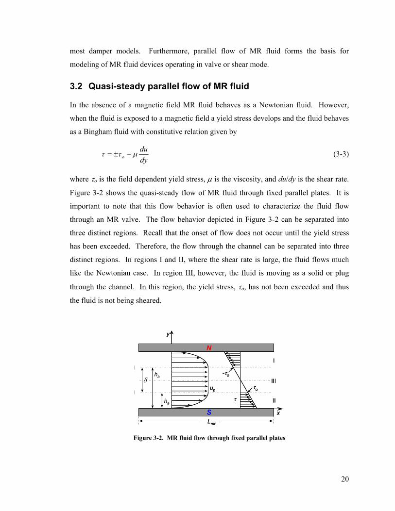
Figure 3-2 shows the quasi-steady flow of MR fluid through fixed parallel plates. It is
important to note that this flow behavior is often used to characterize the fluid flow
through an MR valve. The flow behavior depicted in Figure 3-2 can be separated into
three distinct regions. Recall that the onset of flow does not occur until the yield stress
has been exceeded. Therefore, the flow through the channel can be separated into three
distinct regions. In regions I and II, where the shear rate is large, the fluid flows much
like the Newtonian case. In region III, however, the fluid is moving as a solid or plug
through the channel. In this region, the yield stress, τo, has not been exceeded and thus
the fluid is not being sheared.
x
up
y
Lmr
hb
ha τ
-τo
τo
I
III
II
N
S
δ
x
up
y
Lmr
hb
ha τ
-τo
τo
I
III
II
N
S
δ
Figure 3-2. MR fluid flow through fixed parallel plates
21
Our goal is to determine an expression for the pressure drop caused by the flow
behavior shown in Figure 3-2. The procedure outlined below begins with a reduced form
of the Navier-Stokes equation. By enforcing boundary conditions on both the velocity
and the shear rate, the velocity profile is found in terms of the channel geometry shown in
Figure 3-2. A momentum balance on the fluid yields the plug geometry and allows for
further reduction of the velocity profile. Finally, a cubic expression for the pressure
gradient is found from the flow rate and mean velocity. The solution of this cubic
equation is found in closed form.
3.2.1 Velocity profile
In order to determine the velocity profile, we begin with a reduced form of the Navier-
Stokes equation for one-dimensional flow given by [55]
2
2
yu
xpg
xuu
tu
x ∂∂
+∂∂
−=
∂∂
+∂∂ µρρ (3-4)
Assuming fully developed and horizontal flow, the momentum equation can be further
reduced to
dxdp
dyud
µ1
2
2
= (3-5)
Integration of the momentum equation and enforcing the boundary conditions on shear
rate in each region
( ) 0=ahdydu ahy ≤≤0 (3-6)
0=dydu ba hyh ≤≤ (3-7)
( ) 0=bhdydu hyhb ≤≤ (3-8)
we obtain expressions for the shear rate. Shear rates for regions I and II are found from
equation (3-6) and equation (3-8) as
22
( )ahydxdp
dydu
−=µ1 ahy ≤≤0 (3-9)
( )bhydxdp
dydu
−=µ1 hyhb ≤≤ (3-10)
From the shear rates, the velocity in each region can be found by integrating once more
with respect to y and enforcing the following boundary conditions:
( ) 00 =u ahy ≤≤0 (3-11)
puu = ba hyh ≤≤ (3-12)
( ) 0=hu hyhb ≤≤ (3-13)
From equation (3-11) and equation (3-13), the velocity profiles in regions I and II are
found in terms of the plug geometry as
( )ahyydxdpu 2
21
−=µ
ahy ≤≤0 (3-14)
( ) ( )[ ]hyhhydxdpu b −−−= 2
21 22
µ hyhb ≤≤ (3-15)
3.2.2 Plug geometry
In order to fully define the velocity profile, the three unknowns, ha, hb, and up, must be
found. From either equation (3-14) or equation (3-15), the plug velocity can be found
from the condition uI(ha) = up or uII(hb) = up. Evaluating the velocity in region I at y = ha,
we find an expression for the plug velocity
dxdph
u ap µ2
2
−= (3-16)
An expression for the plug thickness, ab hh −=δ , can be found by enforcing
equilibrium on the plug. Consider the fluid element shown in Figure 3-3. The only
forces acting on the element are due to the pressure gradient and the shear forces acting
on the element.

23
τo(dxdz)
p3(dydz)(p3-∆p)(dydz)
dx
dz
dy
τo(dxdz)
x
y
Lmr
hb
ha τ
-τo
τo
I
III
II
N
S
δ
τo(dxdz)
p3(dydz)(p3-∆p)(dydz)
dx
dz
dy
τo(dxdz)
x
y
Lmr
hb
ha τ
-τo
τo
I
III
II
N
S
δ
Figure 3-3. Balance of forces on a fluid element in the plug region
A balance of forces on the fluid element shown in Figure 3-3 yields
dxdzpdydz oτ2−=∆ (3-17)
where the clockwise rotation of the element due to the shear stress is denoted as positive
[51]. In terms of the plug geometry, equation (3-17) can be written as
odxdp τδ 2−= (3-18)
The plug thickness is then
dxdphh o
abτ
δ2
−=−= (3-19)
Due to the symmetry of the velocity profile we know hb = h – ha and thus from equation
(3-19) we can determine the geometry of the plug as
dxdphh o
aτ
+=2
(3-20)
dxdphh o
bτ
−=2
(3-21)
The velocity profiles can now be written in terms of the known quantities, τo and h, as

24
( ) yhyydxdpu o
µτ
µ−−=
21 ahy ≤≤0 (3-22)
( ) ( )hyhyydxdpu o −+−=
µτ
µ21 hyhb ≤≤ (3-23)
Likewise, the plug velocity can be written as
( )
+−−=
dxdphh
dxdpu oo
pτ
µτ
µ 281 2 (3-24)
The mean velocity through the channel is obtained by integrating the velocity
profile over the thickness of the channel.
∫ ∫ ∫++=∫=a b
a b
h h
h
h
h
h
m udyudyudyh
udyh
u00
11 (3-25)
Recalling that hb = h – ha, we have
( )
−−= 223 34
311
ao
aam hhhhdxdp
hu
µτ
µ (3-26)
Substituting the expression for ha from equation (3-20), an alternative expression for the
mean velocity is found.
( )2
32
31
41
121
dxdphhh
dxdpu o
omτ
µτ
µµ+−−= (3-27)
Note that for τo = 0, equation (3-27) reduces to the mean velocity for the Newtonian case.
Furthermore, should um and τo be known, equation (3-27) results in a third order equation
for the pressure gradient.
04312
3
32
2
3
=−
++
hdxdp
hhu
dxdp oom ττµ
(3-28)
With τo = 0, equation (3-28) reduces to the Newtonian case
2
12hu
dxdp m
N
µ−= (3-29)
25
We also consider the opposite extreme in which flow does not occur due to the formation
of a plug of width h. When h=δ , from equation (3-19) we can write an expression for
the critical pressure drop
hdxdp o
C
τ2−= (3-30)
which is the lowest pressure gradient that would still generate flow between the parallel
plates. Thus, in order to have flow the following condition must be satisfied:
Cdxdp
dxdp
≥ (3-31)
3.2.3 Closed form solution for pressure gradient
In order to solve equation (3-34) for the pressure gradient, we first normalize with respect
to the Newtonian case
012
4123
1323
=
+
+−
µτ
µτ
m
o
Nm
o
N uh
dxdp
dxdp
uh
dxdp
dxdp (3-32)
With the introduction of the following two non-dimensional parameters [51]
µmuh
dxdp
12
2
−=P (3-33)
µτ
m
o
uh
12=T (3-34)
equation (3-32) can be written in the familiar form first presented by Phillips [51].
( ) 0431 323 =++− TPTP (3-35)
The procedure for determining the closed form solution of equation (3-35) is well
documented by Gavin [56], but for completeness, the solution is summarized here. The
solution begins with a transformation of the form
λ−= xP (3-36)
where λ is chosen to be

26
331 T+
−=λ (3-37)
such that the second order term vanishes. The resulting polynomial in x is then
( ) ( ) 031272431
31 3323 =+−++− TTT xx (3-38)
With the definition of the polynomial coefficients
( )23131 T+−=a (3-39)
( )33 312724 TT +−=b (3-40)
equation (3-38) can be written in the standard form
03 =++ baxx (3-41)
In this form, a solution can always be obtained by transforming to the trigonometric
identity [57]
( ) 03coscos3cos4 3 ≡−− θθθ (3-42)
Let θcosmx = , then
( ) 03coscos3cos4coscos 333 ≡−−≡++ θθθθθ bamm (3-43)
Equation (3-43) is always satisfied for
( )bamm
θ3cos343
−=−= (3-44)
It follows then that
32 am −= (3-45)
and
( )am
b33cos =θ (3-46)
27
From equations (3-39) and (3-40), alternative expressions for m and θ can be found as
( )Tm 3132
+= (3-47)
( )
+−= −
3
31
31541cos
31
TTθ (3-48)
from which it follows that
( )( )
+−+= 3
3
31541acos
31cos31
32x
TTT (3-49)
From the transformation in equation (3-36) we find the solution for P
( ) ( )( )
+
+−+=
21
31541acos
31cos31
32
3
3
TTTTP (3-50)
Equation (3-50) provides the solution for the non-dimensional pressure gradient,
P, in terms of the non-dimensional yield stress, T. From this solution, an expression for
the pressure drop in the flow channel can be written in terms of the channel geometry as
mrm L
hu
P 2
12 µτ
P=∆ (3-51)
Equation (3-51) represents the pressure drop developed in the MR valve. This pressure
drop is responsible for the controllability of the MR device.
3.3 Modeling the yield stress
Another important relationship regarding MR fluid behavior is the yield stress as a
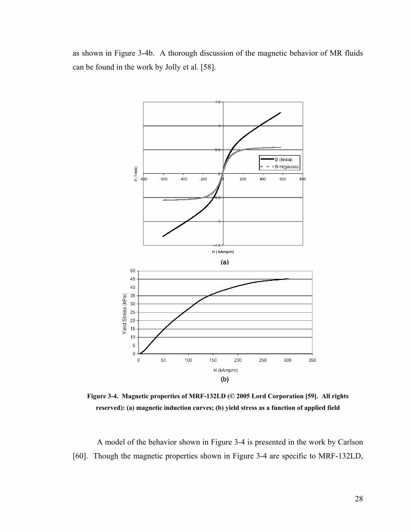
function of applied field strength. It is well known that the yield stress developed in the
fluid increases monotonically with growing magnetic field strength. The yield stress
continues to increase until the fluid reaches magnetic saturation. This is well illustrated
in Figure 3-4. The magnetic induction curve, or B-H curve, shown in Figure 3-4a
indicates that as field strengths increase, the induction, B, approaches saturation. The
saturation observed in magnetic induction is accompanied by a saturation in yield stress
28
as shown in Figure 3-4b. A thorough discussion of the magnetic behavior of MR fluids
can be found in the work by Jolly et al. [58].
(a)
(b)
(a)
(b)
Figure 3-4. Magnetic properties of MRF-132LD (© 2005 Lord Corporation [59]. All rights
reserved): (a) magnetic induction curves; (b) yield stress as a function of applied field
A model of the behavior shown in Figure 3-4 is presented in the work by Carlson
[60]. Though the magnetic properties shown in Figure 3-4 are specific to MRF-132LD,

29
the model proposed by Carlson is general and works for any MR fluid. The proposed
model relates the yield stress to the magnetic field strength as
( )HCo ⋅⋅Φ⋅⋅= 33.6tanh271700 5239.1τ (3-52)
where Φ is the particle loading, and H is the field strength in A/m. The constant C
depends on the carrier fluid and is given as
water16.1oiln hydrocarbo1
oil silicone95.0
===
CCC
Figure 3-5 shows the predicted yield stress as a function of applied field for several MR
fluids available from Lord Corporation. The expression in equation (3-52) accurately
represents the yield stress for each of these fluids.
0 50 100 150 200 250 300 350 400 4500
10
20
30
40
50
60
70
80
90
H (kA/m)
Yie
ld S
tress
(kP
a)
MRF-122EDMRF-132LDMRF-336AGMRF-240BSMRF-241ES
Figure 3-5. Predicted yield stress as a function of applied field
Clearly the model proposed in equation (3-52) is a function of the magnetic field
strength and certain fluid properties. However, the model does not account for the
condition in which the fluid is being used. This model assumes that the yield stress will
30
be developed, regardless of the operating conditions of the fluid. As will be shown in
Chapter 6, this assumption is not valid under certain operating conditions.
3.4 Summary of MR fluid models
With the great number of MR fluid devices and applications, fluid models that offer
accurate representations of the fluid are of great importance. Existing fluid models can
provide insight into the performance of a particular device long before implementation.
However, we must consider the suitability of such models in describing fluid behavior
under adverse operating conditions. Though these extreme operating conditions are
rarely considered, the fluid is often exposed to these conditions in everyday operation of
many MR devices. Existing models, however, may be unsuitable for describing the fluid
behavior under adverse conditions. Both the behavior under adverse operating
conditions, and the model’s ability to represent the fluid under these conditions, will be
addressed in the coming chapters.
31
4 Experimental Approach
The principal objective has been identified as investigating the high velocity and high
shear behavior of MR fluid. Of key importance is the behavior of the fluid itself, not the
behavior of the fluid operating in a particular device. The results must be general such
that they are not specific to a particular device geometry. The simple geometry of the
rheometer allows for the results to be extrapolated to any MR device geometry. To this
end, a rheometer was designed and built which allowed for the high flow testing of MR
fluid. Fluid behavior was to be investigated in the off-state as well as the on-state. As
such, the rheometer had to be designed such that a magnetic field could be applied to the
fluid.
This chapter discusses the design of the slit-flow rheometer. A detailed
description of the design and geometry of the rheometer are provided. Furthermore, a
brief description of the sensors and data acquisition system is also provided. This chapter
concludes by documenting the experimental procedure used in testing.
4.1 Design of slit-flow rheometer
With one of the primary objectives targeted at characterizing MR fluid behavior at high
shear rates, the rheometer needed to be designed in a way that would allow for high
velocity testing. To this end, a Venturi concept was adopted. Exploiting conservation of
mass we are able to use relatively low piston velocities to generate high fluid velocity in
the slit. Consider the schematic shown in Figure 4-1. Conservation requires that flow
rate be maintained. Thus, the velocity exiting the Venturi is proportional to v1 as
12
12 v
AAv = (4-1)
As the area ratio increases, the velocity at the exit increases. This simple property is
exploited in the design of the rheometer.

32
A2
v1
A1
v2
A2
v1
A1
v2
Figure 4-1. Venturi schematic
The overall assembly of the slit-flow rheometer is shown in Figure 4-2. Several
primary components are identified: the main bore, the reducer, the flow channel, the
electromagnet, the actuator, and the fill reservoir. Figure 4-2b also shows the
thermocouple used to measure fluid temperature and the Hall probe used to measure the
field strength. Each of these components will be discussed in detail in the following
sections.
101.6 mm bore
Reducer
1x10 mm slit
Hall Probe Electromagnet
ThermocoupleRheometer
MTS Actuator
Fill Reservoir
(a) (b)
101.6 mm bore
Reducer
1x10 mm slit
Hall Probe Electromagnet
ThermocoupleRheometer
MTS Actuator
Fill Reservoir
(a) (b)
Figure 4-2. (a) MR rheometer mounted in MTS load frame; (b) Close-up of MR rheometer
33
The hydraulic actuator used in this study is an MTS axial/torsion actuator with a
force capacity of 490 kN (110 kips). Because the actuator is bottom actuated, the
rheometer was designed to allow for bottom actuation. The framing shown in Figure
4-2b allows the actuation to occur from the bottom. In other words, the entire capillary
rheometer moves while the piston is held in place. The actuator force is transmitted
through the 25.4 mm thick steel base plate, then through the four steel pipes, into the
main tube flange which reacts against the piston, driving the fluid through the flow
channel.
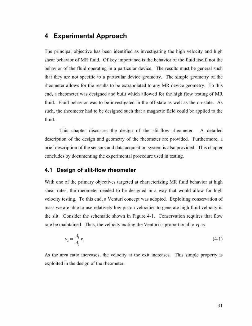
In order to achieve a large area ratio, the main tube was chosen to have a 101.6
mm (4 inch) bore. The main tube (Figure 4-3) is 4.5" OD by 4.0" ID honed DOM steel,
supplied by Scot Industries Inc. When assembled, the area ratio of the rheometer is
greater than 1000. A 25.4 mm (1 inch) thick steel flange is welded to the end of the tube
so that it can be bolted to the reducing section. A fiber gasket rated at 5000 psi is used to
seal the connection between the main tube and the reducing section. The tube length is
222.25 mm (8.75"). This length is limited by the stroke of the hydraulic actuator being
used in this study. A longer tube is desirable because it allows for multiple tests in a
single stroke. It should be noted that the main tube is free of holes along its length.
Holes along the length of the tube are undesirable as they can damage piston seals.
Figure 4-3. Main tube
The piston that was used to drive the fluid through the rheometer was made from
7075-T6 aluminum. Figure 4-4 shows the piston along with the nylon bushing. The

34
nylon bushing serves merely as a second point of contact to support any lateral loading.
A polyurethane or Viton® o-ring serves as the dynamic seal in the rheometer. The two
holes in the piston were designed to allow for top filling of the capillary rheometer. Top
filling the rheometer prolonged the life of the seals because the main bore was free of
holes or other obstructions. The piston rod was a 22.23 mm (7/8") OD hardened
precision steel shaft.
Figure 4-4. Piston with Viton® o-ring and nylon bushing
The reducer was designed to reduce the diameter from the 101.6 mm bore of the
main tube to the 10 mm width of the flow channel. For ease of machining, the reducer
was made from 7075-T6 aluminum. The length of the reducer was chosen such that the
included angle was less than 50 degrees. An included angle of 50 degrees along with an
area ratio (A2/A1) of ~0.01 results is a head loss coefficient less than 0.1 [61]. The
reducer is shown in Figure 4-5. It should be noted that the reducer was made from two
independent parts. Again, to simplify the machining, two reducers were made, one
reducing the diameter from 101.6 mm to 50.8 mm, and the other reducing the diameter
from 50.8 mm to 10 mm. Here again, a fiber gasket is used to seal the connection.
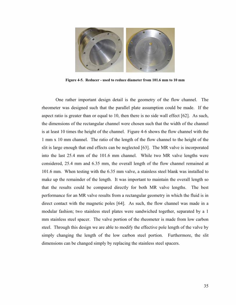
35
Figure 4-5. Reducer - used to reduce diameter from 101.6 mm to 10 mm
One rather important design detail is the geometry of the flow channel. The
rheometer was designed such that the parallel plate assumption could be made. If the
aspect ratio is greater than or equal to 10, then there is no side wall effect [62]. As such,
the dimensions of the rectangular channel were chosen such that the width of the channel
is at least 10 times the height of the channel. Figure 4-6 shows the flow channel with the
1 mm x 10 mm channel. The ratio of the length of the flow channel to the height of the
slit is large enough that end effects can be neglected [63]. The MR valve is incorporated
into the last 25.4 mm of the 101.6 mm channel. While two MR valve lengths were
considered, 25.4 mm and 6.35 mm, the overall length of the flow channel remained at
101.6 mm. When testing with the 6.35 mm valve, a stainless steel blank was installed to
make up the remainder of the length. It was important to maintain the overall length so
that the results could be compared directly for both MR valve lengths. The best
performance for an MR valve results from a rectangular geometry in which the fluid is in
direct contact with the magnetic poles [64]. As such, the flow channel was made in a
modular fashion; two stainless steel plates were sandwiched together, separated by a 1
mm stainless steel spacer. The valve portion of the rheometer is made from low carbon
steel. Through this design we are able to modify the effective pole length of the valve by
simply changing the length of the low carbon steel portion. Furthermore, the slit
dimensions can be changed simply by replacing the stainless steel spacers.
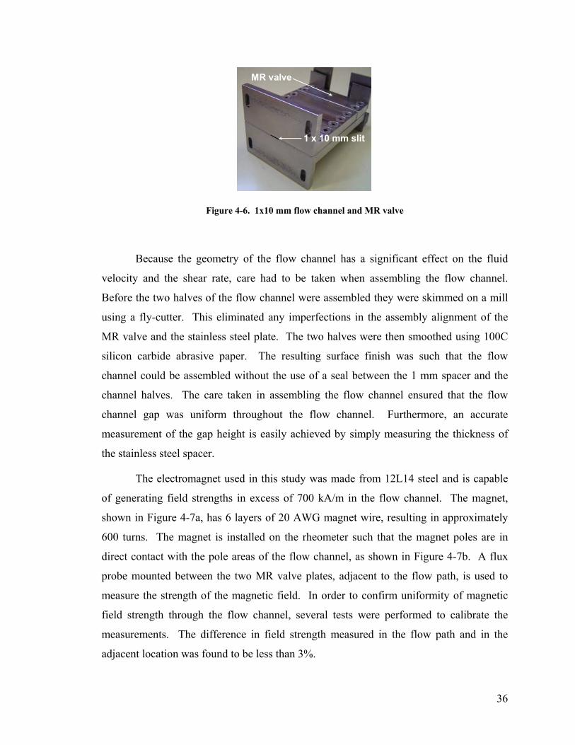
36
MR valve
1 x 10 mm slit
MR valve
1 x 10 mm slit
Figure 4-6. 1x10 mm flow channel and MR valve
Because the geometry of the flow channel has a significant effect on the fluid
velocity and the shear rate, care had to be taken when assembling the flow channel.
Before the two halves of the flow channel were assembled they were skimmed on a mill
using a fly-cutter. This eliminated any imperfections in the assembly alignment of the
MR valve and the stainless steel plate. The two halves were then smoothed using 100C
silicon carbide abrasive paper. The resulting surface finish was such that the flow
channel could be assembled without the use of a seal between the 1 mm spacer and the
channel halves. The care taken in assembling the flow channel ensured that the flow
channel gap was uniform throughout the flow channel. Furthermore, an accurate
measurement of the gap height is easily achieved by simply measuring the thickness of
the stainless steel spacer.
The electromagnet used in this study was made from 12L14 steel and is capable
of generating field strengths in excess of 700 kA/m in the flow channel. The magnet,
shown in Figure 4-7a, has 6 layers of 20 AWG magnet wire, resulting in approximately
600 turns. The magnet is installed on the rheometer such that the magnet poles are in
direct contact with the pole areas of the flow channel, as shown in Figure 4-7b. A flux
probe mounted between the two MR valve plates, adjacent to the flow path, is used to
measure the strength of the magnetic field. In order to confirm uniformity of magnetic
field strength through the flow channel, several tests were performed to calibrate the
measurements. The difference in field strength measured in the flow path and in the
adjacent location was found to be less than 3%.

37
(a) (b)
ElectromagnetFlux probe
(a) (b)
ElectromagnetFlux probe
Figure 4-7. Electromagnet used to activate MR fluid
4.2 Data acquisition system
This section describes the data acquisition system used in the experiments. Both the
hardware and software components are discussed. Hardware components include various
sensors, controllers, and power supplies. The software components include the MTS
TestStar II software and dSPACE Control Desk.
4.2.1 Hardware components
As mentioned earlier, a Hall probe was used to measure magnetic field strength. The
probe itself was an “ultra-thin” (0.2 mm x 1.5 mm) transverse probe from F. W. Bell.
This probe was connected to an F. W. Bell 5080 Gauss-meter. The probe and meter are
shown in Figure 4-8. The 5080 model provides an analog output for recording the field
strength. With a ±3 V full-scale output, the field strength could be recorded for each
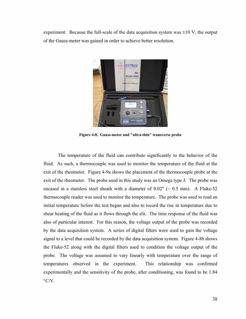
38
experiment. Because the full-scale of the data acquisition system was ±10 V, the output
of the Gauss-meter was gained in order to achieve better resolution.
Figure 4-8. Gauss-meter and "ultra-thin" transverse probe
The temperature of the fluid can contribute significantly to the behavior of the
fluid. As such, a thermocouple was used to monitor the temperature of the fluid at the
exit of the rheometer. Figure 4-9a shows the placement of the thermocouple probe at the
exit of the rheometer. The probe used in this study was an Omega type J. The probe was
encased in a stainless steel sheath with a diameter of 0.02" (~ 0.5 mm). A Fluke-52
thermocouple reader was used to monitor the temperature. The probe was used to read an
initial temperature before the test began and also to record the rise in temperature due to
shear heating of the fluid as it flows through the slit. The time response of the fluid was
also of particular interest. For this reason, the voltage output of the probe was recorded
by the data acquisition system. A series of digital filters were used to gain the voltage
signal to a level that could be recorded by the data acquisition system. Figure 4-8b shows
the Fluke-52 along with the digital filters used to condition the voltage output of the
probe. The voltage was assumed to vary linearly with temperature over the range of
temperatures observed in the experiment. This relationship was confirmed
experimentally and the sensitivity of the probe, after conditioning, was found to be 1.84
°C/V.

39
Flow channel exit
Thermocouple(a) (b)
Flow channel exit
Thermocouple
Flow channel exit
Thermocouple(a) (b)
Figure 4-9. Fluid temperature measurements: (a) thermocouple probe mounted at exit of rheometer;
(b) Fluke-52 and digital filters used to monitor fluid temperature
The magnet was controlled from within Control Desk. The circuit box and power
supplies shown in Figure 4-10 were used to amplify the signal from Control Desk. The
circuit box is a current driver circuit which receives input from Control Desk and drives a
proportional current through the magnet. The ±15 V power supply is used to power the
circuit. The 12 V power supply is used to amplify the output of the circuit to power the
magnet.
Figure 4-10. Circuit box and power supplies used to power the electromagnet
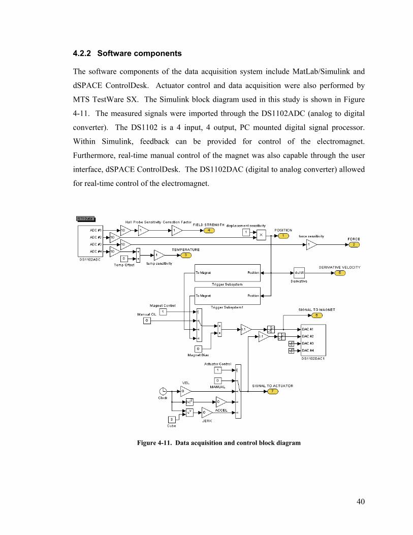
40
4.2.2 Software components
The software components of the data acquisition system include MatLab/Simulink and
dSPACE ControlDesk. Actuator control and data acquisition were also performed by
MTS TestWare SX. The Simulink block diagram used in this study is shown in Figure
4-11. The measured signals were imported through the DS1102ADC (analog to digital
converter). The DS1102 is a 4 input, 4 output, PC mounted digital signal processor.
Within Simulink, feedback can be provided for control of the electromagnet.
Furthermore, real-time manual control of the magnet was also capable through the user
interface, dSPACE ControlDesk. The DS1102DAC (digital to analog converter) allowed
for real-time control of the electromagnet.
Figure 4-11. Data acquisition and control block diagram
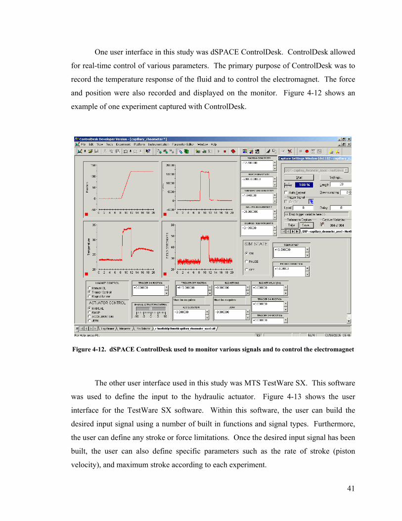
41
One user interface in this study was dSPACE ControlDesk. ControlDesk allowed
for real-time control of various parameters. The primary purpose of ControlDesk was to
record the temperature response of the fluid and to control the electromagnet. The force
and position were also recorded and displayed on the monitor. Figure 4-12 shows an
example of one experiment captured with ControlDesk.
Figure 4-12. dSPACE ControlDesk used to monitor various signals and to control the electromagnet
The other user interface used in this study was MTS TestWare SX. This software
was used to define the input to the hydraulic actuator. Figure 4-13 shows the user
interface for the TestWare SX software. Within this software, the user can build the
desired input signal using a number of built in functions and signal types. Furthermore,
the user can define any stroke or force limitations. Once the desired input signal has been
built, the user can also define specific parameters such as the rate of stroke (piston
velocity), and maximum stroke according to each experiment.

42
Figure 4-13. MTS TestWare SX software used to control hydraulic actuator
4.3 Experiment procedures
Through the experiment we hope to identify the performance of MR fluid at high
velocities. Velocity and magnetic field strength are the only variables. Defining the
piston velocity, a corresponding fluid velocity in the flow channel can be calculated from
the area ratio. A ramp signal is used as the input to the system. This constant velocity
input ensures that the force reaches steady-state, and that the flow is steady flow. In
order to avoid any transient loading associated with the MR fluid yield stress, a trigger is
used to turn on the electromagnet, only after the fluid has begun to flow. It is relatively
important that the fluid be in an amorphous state before testing begins. Otherwise, large
transient forces can occur.

43
Figure 4-14 shows the input used during testing. The piston velocity, vp, and the
stroke are defined in the TestWare SX software. Once the actuator position reaches a
predetermined value, normally 5 mm, the electromagnet is turned on. At 5 mm from the
end of the stroke, the electromagnet is turned off to prevent the fluid particles from being
in an energized state when the fluid is not flowing. Once the actuator reaches the
maximum stroke, the program is paused. The program waits for the user to resume
testing. The pause is used to open a breather valve so when the actuator is lowered to its
initial position, air is not drawn in through the bottom of the rheometer. The test is
repeated for each velocity and magnetic field strength. With a large stroke and low
piston velocities, it is possible to run several velocities before reaching the stroke limit.
This is the advantage of having a large stroke.
Time
Position
Pmax
ton toff
vp
Pon
Poff
Time
Position
Pmax
ton toff
vp
Pon
Poff
Figure 4-14. Ramp input used in steady flow experiments
Piston velocities considered in this study ranged from 2 mm/s to 36 mm/s (~ 0.1
in/s – 1.4 in/s). With the 1x10 mm flow channel geometry, these piston velocities
correspond to fluid velocities ranging from 2 m/s to 37 m/s (~ 6.7 ft/s – 121 ft/s). The
maximum shear rate achieved is 2.5x10⁵ s-1. For each velocity several magnetic field
strengths were considered, ranging from 100 kA/m to 200 kA/m. For all velocities the
fluid was also characterized in the absence of a magnetic field.

44
4.4 Friction force
Before the fluid was run through the rheometer, it was necessary to determine the friction
force inherent in the system. This force must be accounted for when calculating the shear
stress and the viscosity of the fluid. Sources of friction include the contact between the
piston rod and the nylon bushing as well as the dynamic seal between the o-ring and the
cylinder wall. To characterize these sources of friction, the rheometer was run without
fluid. The slit-flow portion of the rheometer was removed to eliminate any air pressure
that may be generated at high velocities. Several piston velocities were run and the force
was measured at each velocity. It should be noted that though the rheometer was empty,
the cylinder walls were lubricated. This was done in order to avoid dry friction between
the Viton® o-ring and the cylinder walls.
Figure 4-15 shows the friction force as a function of piston velocity. The results
indicate that friction is a function of piston velocity. In order to eliminate friction from
the analysis of the fluid results, an accurate model for the friction as a function of piston
velocity was required. An expression well suited to describe the velocity dependent
friction was found to be
2464.03565.0 −⋅= pfr vF (4-2)
and is shown along with the experimental data in Figure 4-15.
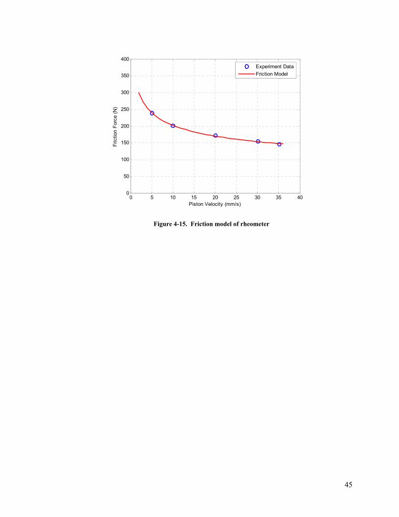
45
0 5 10 15 20 25 30 35 400
50
100
150
200
250
300
350
400
Piston Velocity (mm/s)
Fric
tion
Forc
e (N
)
Experiment DataFriction Model
Figure 4-15. Friction model of rheometer
46
5 Off-State Behavior of MR Fluid at High Shear Rates
Though much of the success of MR fluids can be attributed to the controllable or on-state
behavior of the fluid, the off-state behavior of the fluid cannot be overlooked. Much of
the literature tends to focus on the behavior of the fluid when exposed to a magnetic field.
However, the success of many MR fluid applications is highly dependent on the off-state
behavior of the fluid. Furthermore, much of the published data for MR fluids is limited
to shear rates and flow velocities that do not completely encompass the environment to
which an MR fluid is exposed in an MR device. As such, this chapter examines the
behavior of MR fluid in the absence of a magnetic field when subjected to extreme flow
conditions, i.e., high shear rates.
The chapter begins with a discussion of the composition of MR fluids. Several
factors contribute to the rheological properties of MR fluids. Such factors include
concentration and density of particles, particle size and shape distribution, properties of
the carrier fluid, additional additives, applied field, temperature, and others. The specific
physical properties of MRF-132LD are discussed. Because the behavior of the fluid is
highly dependent on the carrier, or host fluid, a characterization of the host fluid is
presented. High shear behavior is identified first for the carrier fluid and then for the MR
fluid. The high shear viscosity is found for each fluid and, based on the shear stress
versus shear rate relationship, a model is proposed for each fluid. The chapter concludes
with a discussion of temperature response of the fluid during the high flow experiments.
5.1 Magnetorheological fluid composition
Magnetorheological fluids are non-colloidal suspensions of micron-sized, magnetically
polarizable particles. Typical particle diameter is 3-5 µm. As such, MR fluids should not
be confused with colloidal ferrofluids in which the particles are 1000 times smaller. In
contrast, MR fluids with larger particles have also been considered. Lord Corporation’s
180 kN seismic damper employs an MR fluid with particles ranging in size from 0.1 µm
to 500 µm, with a preferred size between 1 µm and 100 µm [65]. As particle size
increases, however, suspension within the fluid becomes a challenge. This challenge is
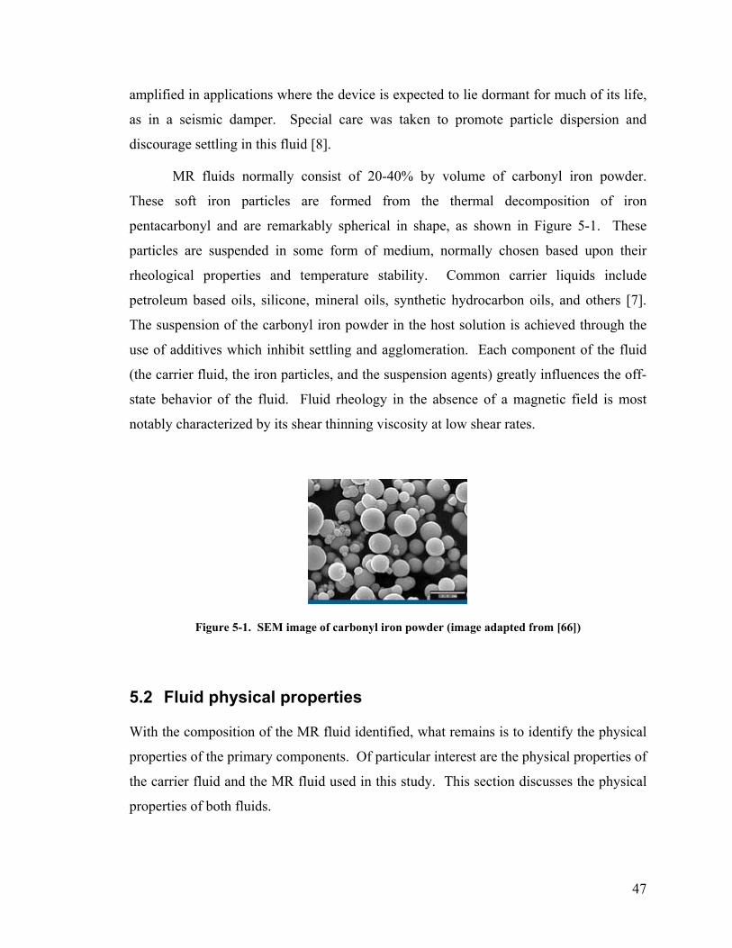
47
amplified in applications where the device is expected to lie dormant for much of its life,
as in a seismic damper. Special care was taken to promote particle dispersion and
discourage settling in this fluid [8].
MR fluids normally consist of 20-40% by volume of carbonyl iron powder.
These soft iron particles are formed from the thermal decomposition of iron
pentacarbonyl and are remarkably spherical in shape, as shown in Figure 5-1. These
particles are suspended in some form of medium, normally chosen based upon their
rheological properties and temperature stability. Common carrier liquids include
petroleum based oils, silicone, mineral oils, synthetic hydrocarbon oils, and others [7].
The suspension of the carbonyl iron powder in the host solution is achieved through the
use of additives which inhibit settling and agglomeration. Each component of the fluid
(the carrier fluid, the iron particles, and the suspension agents) greatly influences the off-
state behavior of the fluid. Fluid rheology in the absence of a magnetic field is most
notably characterized by its shear thinning viscosity at low shear rates.
Figure 5-1. SEM image of carbonyl iron powder (image adapted from [66])
5.2 Fluid physical properties
With the composition of the MR fluid identified, what remains is to identify the physical
properties of the primary components. Of particular interest are the physical properties of
the carrier fluid and the MR fluid used in this study. This section discusses the physical
properties of both fluids.

48
5.2.1 Carrier fluid properties
As mention earlier, the behavior of MR fluid is greatly influenced by the carrier fluid. In
fact, at high shear rates, the carrier fluid and suspension agents dominate the behavior [8].
As such, the properties of the carrier fluid should be well understood. The specific host
fluid used in MRF-132LD is a synthetic hydrocarbon base oil, called Oronite Synfluid 4
cSt PAO, supplied by the Chevron Phillips Chemical Company in Houston Texas. The
physical and chemical properties are taken from the MSDS and are shown in Table 5-1.
According to the MSDS, the fluid’s kinematic viscosity is 16 cSt, or 0.16 cm2/s. The
relationship between kinematic viscosity, ν, and dynamic viscosity, µ, is defined as
ρµν = (5-1)
where ρ is the fluid density found from the specific gravity. With a specific gravity of
0.82, the dynamic viscosity is 0.0123 Pa-s. As a point of reference, it is important to note
that this viscosity was measured at a temperature of nearly 40 °C as indicated in Table
5-1.
Table 5-1. Physical and chemical properties of carrier fluid (adapted from [67])
Vapor Pressure 1.7 mmHg @ 177 °C
Vapor Density (Air = 1) > 10
Boiling Point 414 °C
Solubility Soluble in hydrocarbon solvents; insoluble in water
Specific Gravity 0.82 @ 15.6 °C
Kinematic Viscosity 16 cSt @ 37.8 °C
Pour Point -73 °C
5.2.2 MRF-132LD properties
The specific type of MR fluid used in this study is Lord Corporation’s MRF-132LD.
This particular fluid is a hydrocarbon-based MR fluid containing 32% iron by volume.
The average particle diameter for this fluid is 3 µm [7]. Basic physical properties of the
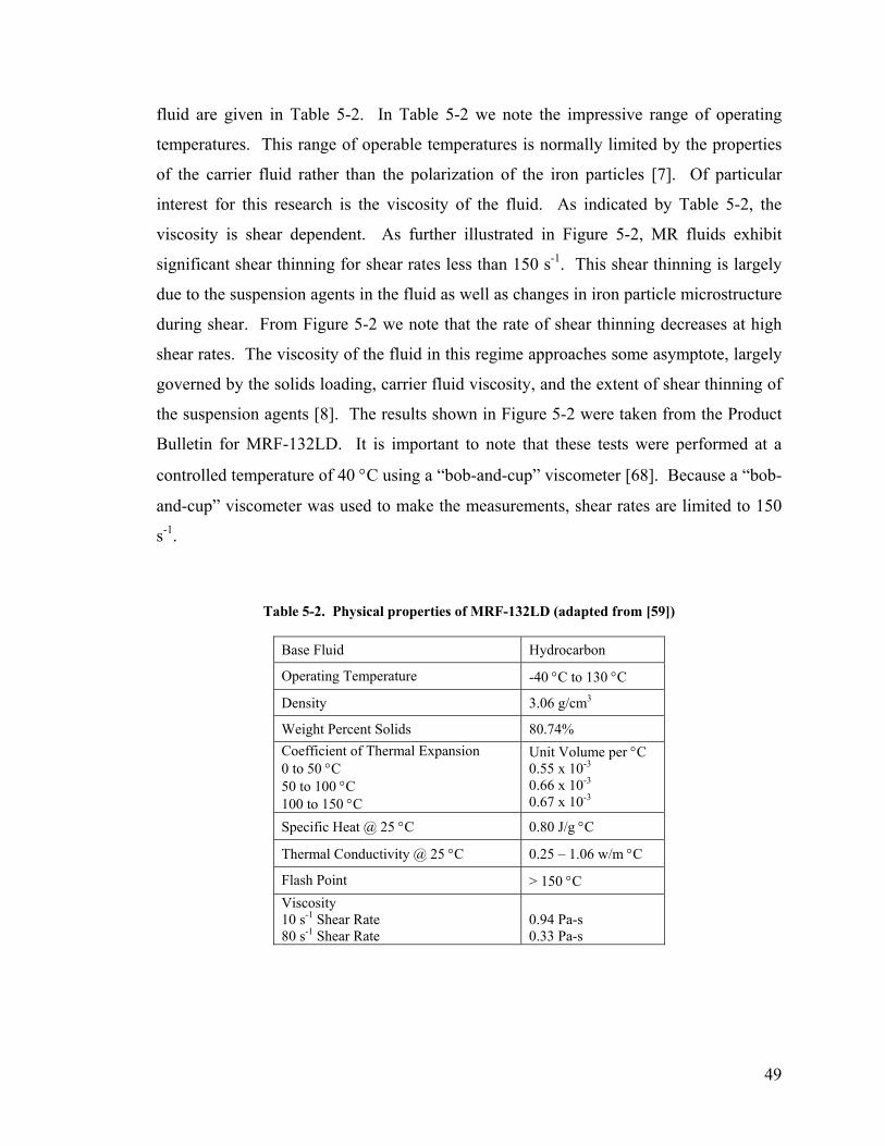
49
fluid are given in Table 5-2. In Table 5-2 we note the impressive range of operating
temperatures. This range of operable temperatures is normally limited by the properties
of the carrier fluid rather than the polarization of the iron particles [7]. Of particular
interest for this research is the viscosity of the fluid. As indicated by Table 5-2, the
viscosity is shear dependent. As further illustrated in Figure 5-2, MR fluids exhibit
significant shear thinning for shear rates less than 150 s-1. This shear thinning is largely
due to the suspension agents in the fluid as well as changes in iron particle microstructure
during shear. From Figure 5-2 we note that the rate of shear thinning decreases at high
shear rates. The viscosity of the fluid in this regime approaches some asymptote, largely
governed by the solids loading, carrier fluid viscosity, and the extent of shear thinning of
the suspension agents [8]. The results shown in Figure 5-2 were taken from the Product
Bulletin for MRF-132LD. It is important to note that these tests were performed at a
controlled temperature of 40 °C using a “bob-and-cup” viscometer [68]. Because a “bob-
and-cup” viscometer was used to make the measurements, shear rates are limited to 150
s-1.
Table 5-2. Physical properties of MRF-132LD (adapted from [59])
Base Fluid Hydrocarbon
Operating Temperature -40 °C to 130 °C
Density 3.06 g/cm3
Weight Percent Solids 80.74% Coefficient of Thermal Expansion 0 to 50 °C 50 to 100 °C 100 to 150 °C
Unit Volume per °C 0.55 x 10⁻³ 0.66 x 10⁻³ 0.67 x 10⁻³
Specific Heat @ 25 °C 0.80 J/g °C
Thermal Conductivity @ 25 °C 0.25 – 1.06 w/m °C
Flash Point > 150 °C Viscosity 10 s-1 Shear Rate 80 s-1 Shear Rate
0.94 Pa-s 0.33 Pa-s
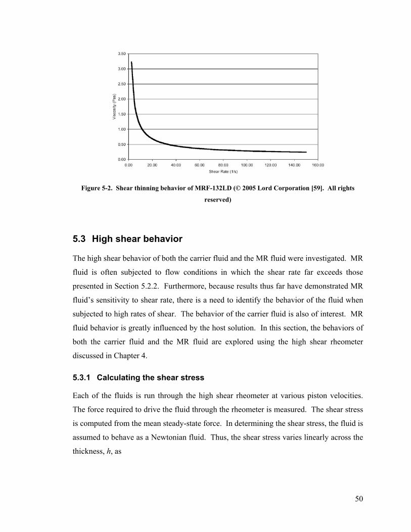
50
Figure 5-2. Shear thinning behavior of MRF-132LD (© 2005 Lord Corporation [59]. All rights
reserved)
5.3 High shear behavior
The high shear behavior of both the carrier fluid and the MR fluid were investigated. MR
fluid is often subjected to flow conditions in which the shear rate far exceeds those
presented in Section 5.2.2. Furthermore, because results thus far have demonstrated MR
fluid’s sensitivity to shear rate, there is a need to identify the behavior of the fluid when
subjected to high rates of shear. The behavior of the carrier fluid is also of interest. MR
fluid behavior is greatly influenced by the host solution. In this section, the behaviors of
both the carrier fluid and the MR fluid are explored using the high shear rheometer
discussed in Chapter 4.
5.3.1 Calculating the shear stress
Each of the fluids is run through the high shear rheometer at various piston velocities.
The force required to drive the fluid through the rheometer is measured. The shear stress
is computed from the mean steady-state force. In determining the shear stress, the fluid is
assumed to behave as a Newtonian fluid. Thus, the shear stress varies linearly across the
thickness, h, as
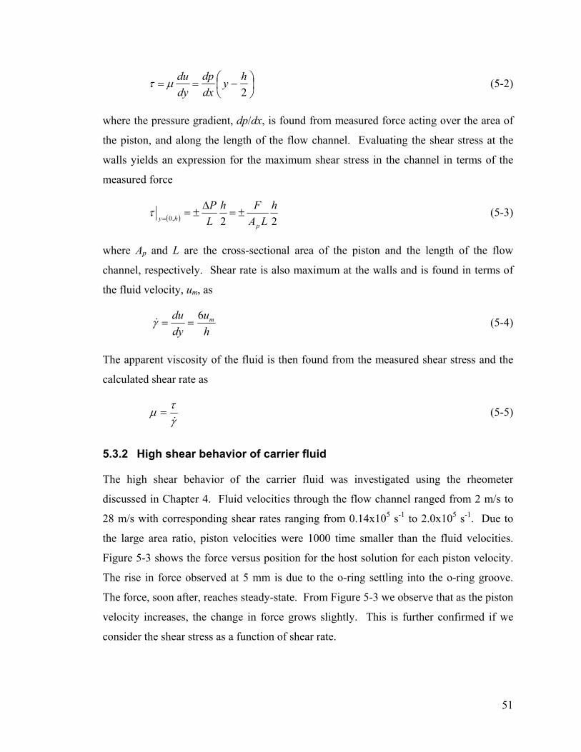
51
−==
2hy
dxdp
dyduµτ (5-2)
where the pressure gradient, dp/dx, is found from measured force acting over the area of
the piston, and along the length of the flow channel. Evaluating the shear stress at the
walls yields an expression for the maximum shear stress in the channel in terms of the
measured force
( ) 22,0
hLA
FhLP
phy
±=∆
±==
τ (5-3)
where Ap and L are the cross-sectional area of the piston and the length of the flow
channel, respectively. Shear rate is also maximum at the walls and is found in terms of
the fluid velocity, um, as
hu
dydu m6
==γ& (5-4)
The apparent viscosity of the fluid is then found from the measured shear stress and the
calculated shear rate as
γτµ&
= (5-5)
5.3.2 High shear behavior of carrier fluid
The high shear behavior of the carrier fluid was investigated using the rheometer
discussed in Chapter 4. Fluid velocities through the flow channel ranged from 2 m/s to
28 m/s with corresponding shear rates ranging from 0.14x10⁵ s-1 to 2.0x10⁵ s-1. Due to
the large area ratio, piston velocities were 1000 time smaller than the fluid velocities.
Figure 5-3 shows the force versus position for the host solution for each piston velocity.
The rise in force observed at 5 mm is due to the o-ring settling into the o-ring groove.
The force, soon after, reaches steady-state. From Figure 5-3 we observe that as the piston
velocity increases, the change in force grows slightly. This is further confirmed if we
consider the shear stress as a function of shear rate.

52
-10 0 10 20 30 40 50 60 70 800
2
4
6
8
10
12
14
Position (mm)
Forc
e (k
N)
2 mm/s4 mm/s6 mm/s8 mm/s10 mm/s12 mm/s14 mm/s16 mm/s
18 mm/s
20 mm/s
22 mm/s
24 mm/s
26 mm/s
28 mm/s
Figure 5-3. Force versus position for carrier fluid
From the mean steady-state force, the shear stress is found from equation (5-3).
Figure 5-4a shows the shear stress as a function of shear rate for the carrier fluid. In
Figure 5-4 (a) we note that the behavior is not quite Newtonian. A moderate shear
thickening is observed for growing shear rates. This behavior is better illustrated if we
consider the fluid shear viscosity as a function of shear rate, as shown in Figure 5-4b.
The apparent viscosity was defined in equation (5-5) as the measured shear stress divided
by the shear rate. Figure 5-4b further demonstrates the shear thickening behavior of the
carrier fluid. As a point of reference, it is noted that these experiments were performed at
room temperature. Furthermore, fluid initial temperature measurements had a mean
value of 24.4 °C. At this temperature, experiments yielded a mean fluid viscosity of 0.03
Pa-s.
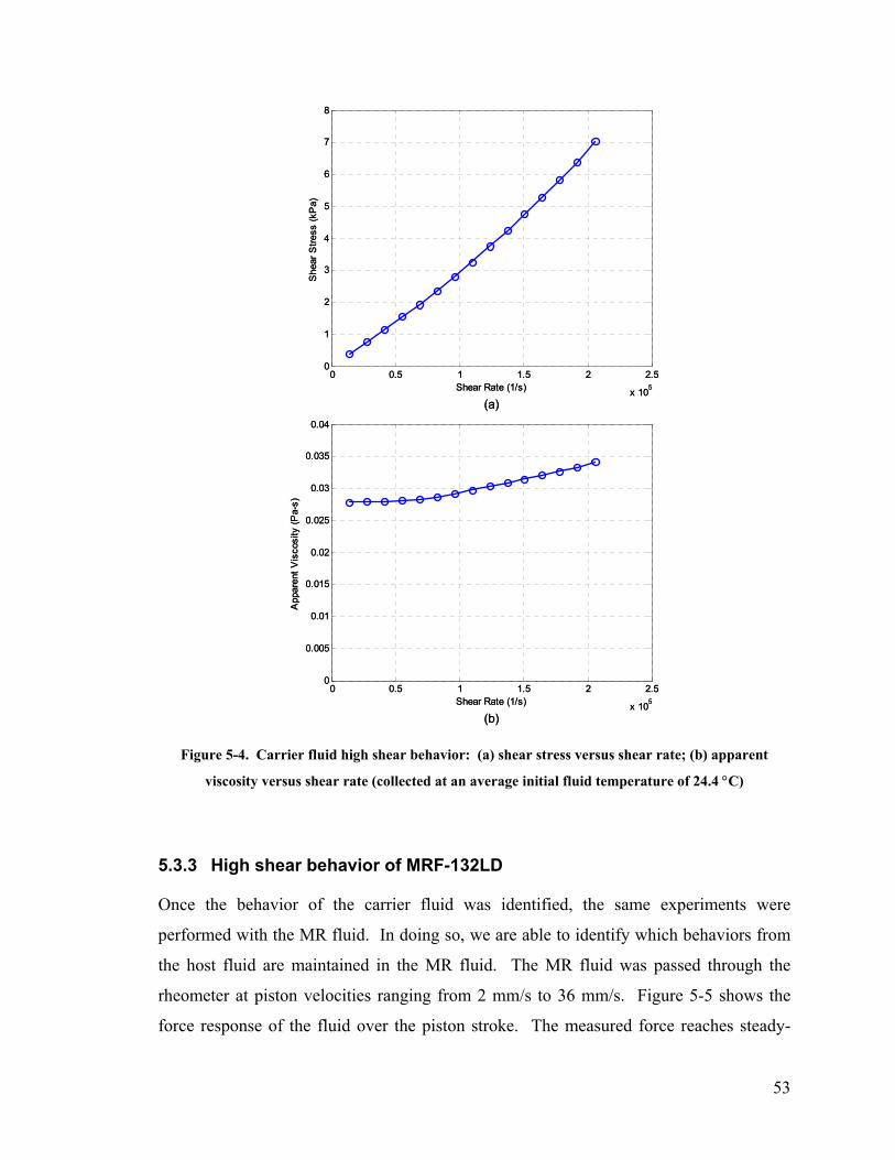
53
(a)
(b)
0 0.5 1 1.5 2 2.5
x 105
0
1
2
3
4
5
6
7
8
Shear Rate (1/s)
She
ar S
tress
(kP
a)
0 0.5 1 1.5 2 2.5
x 105
0
0.005
0.01
0.015
0.02
0.025
0.03
0.035
0.04
Shear Rate (1/s)
App
aren
t Vis
cosi
ty (P
a-s)
(a)
(b)
0 0.5 1 1.5 2 2.5
x 105
0
1
2
3
4
5
6
7
8
Shear Rate (1/s)
She
ar S
tress
(kP
a)
0 0.5 1 1.5 2 2.5
x 105
0
0.005
0.01
0.015
0.02
0.025
0.03
0.035
0.04
Shear Rate (1/s)
App
aren
t Vis
cosi
ty (P
a-s)
Figure 5-4. Carrier fluid high shear behavior: (a) shear stress versus shear rate; (b) apparent
viscosity versus shear rate (collected at an average initial fluid temperature of 24.4 °C)
5.3.3 High shear behavior of MRF-132LD
Once the behavior of the carrier fluid was identified, the same experiments were
performed with the MR fluid. In doing so, we are able to identify which behaviors from
the host fluid are maintained in the MR fluid. The MR fluid was passed through the
rheometer at piston velocities ranging from 2 mm/s to 36 mm/s. Figure 5-5 shows the
force response of the fluid over the piston stroke. The measured force reaches steady-

54
state after a stroke of 40 mm. The slight roll-off in force observed at higher piston
velocities may be attributed to increased fluid temperature during testing. As with the
carrier fluid, the shear stress is found from the mean steady-state force.
-20 0 20 40 60 80 100 120 1400
10
20
30
40
50
60
70
80
Position (mm)
Forc
e (k
N)
2 mm/s
6 mm/s
10 mm/s
14 mm/s
18 mm/s
22 mm/s
26 mm/s
30 mm/s
34 mm/s
Figure 5-5. Force versus position for MR fluid
Plotting the shear stress versus shear rate, we see that the MR fluid behavior is
quite Newtonian. Figure 5-6a shows the shear stress as a function of shear rate. The
apparent viscosity, shown in Figure 5-6b, is found at each shear rate. While a moderate
shear thinning is observed at lower shear rates, the viscosity seems to reach equilibrium
at 0.14 Pa-s. However, close inspection reveals a slight increase in viscosity for higher
rates of shear. This behavior is consistent with the behavior observed in the carrier fluid.
While the viscosity is quite different in magnitude, the shear thickening behavior may be
largely governed by the carrier fluid. Again, as a point of reference, it is noted that these
experiments were performed at room temperature. On this particular occasion, the mean
fluid initial temperature was 25.8 °C. At this temperature, the mean fluid viscosity is
0.142 Pa-s.

55
(a)
(b)
0 0.5 1 1.5 2 2.5
x 105
0
5
10
15
20
25
30
35
40
Shear Rate (1/s)
She
ar S
tress
(kP
a)
0 0.5 1 1.5 2 2.5
x 105
0
0.02
0.04
0.06
0.08
0.1
0.12
0.14
0.16
0.18
Shear Rate (1/s)
App
aren
t Vis
cosi
ty (P
a-s)
(a)
(b)
0 0.5 1 1.5 2 2.5
x 105
0
5
10
15
20
25
30
35
40
Shear Rate (1/s)
She
ar S
tress
(kP
a)
0 0.5 1 1.5 2 2.5
x 105
0
0.02
0.04
0.06
0.08
0.1
0.12
0.14
0.16
0.18
Shear Rate (1/s)
App
aren
t Vis
cosi
ty (P
a-s)
Figure 5-6. MR fluid high shear behavior: (a) shear stress versus shear rate; (b) apparent viscosity
versus shear rate (collected at an average initial fluid temperature of 25.8 °C)
5.4 Reynolds number
In order to be thorough, the results presented in Section 5.3 should include a discussion
of the Reynolds number. Flowing at high velocities, there may be some concern that the
fluid flow is not laminar and that the methods used to determine the shear stress and
viscosity are not valid. To assuage this concern, the Reynolds number was calculated for
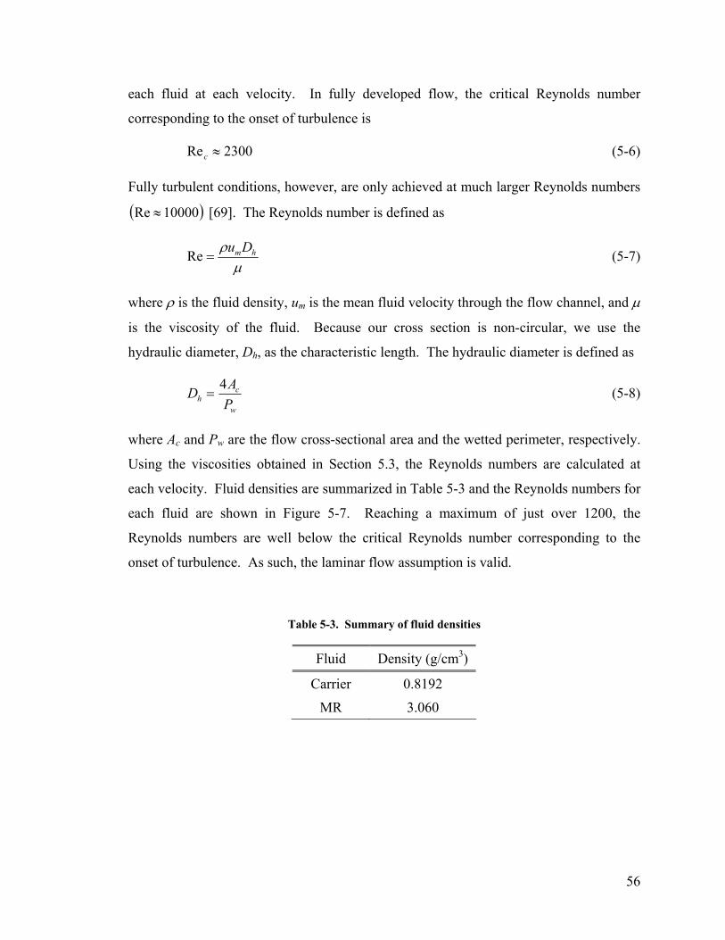
56
each fluid at each velocity. In fully developed flow, the critical Reynolds number
corresponding to the onset of turbulence is
2300Re ≈c (5-6)
Fully turbulent conditions, however, are only achieved at much larger Reynolds numbers
( )10000Re ≈ [69]. The Reynolds number is defined as
µρ hmDu
=Re (5-7)
where ρ is the fluid density, um is the mean fluid velocity through the flow channel, and µ
is the viscosity of the fluid. Because our cross section is non-circular, we use the
hydraulic diameter, Dh, as the characteristic length. The hydraulic diameter is defined as
w
ch P
AD 4= (5-8)
where Ac and Pw are the flow cross-sectional area and the wetted perimeter, respectively.
Using the viscosities obtained in Section 5.3, the Reynolds numbers are calculated at
each velocity. Fluid densities are summarized in Table 5-3 and the Reynolds numbers for
each fluid are shown in Figure 5-7. Reaching a maximum of just over 1200, the
Reynolds numbers are well below the critical Reynolds number corresponding to the
onset of turbulence. As such, the laminar flow assumption is valid.
Table 5-3. Summary of fluid densities
Fluid Density (g/cm3)
Carrier 0.8192
MR 3.060

57
0 5 10 15 20 25 30 35 400
200
400
600
800
1000
1200
1400
Fluid Velocity (m/s)
Rey
nold
s N
umbe
r
Carrier FluidMR Fluid
Figure 5-7. Reynolds number for carrier fluid and MR fluid
5.5 Fluid behavior models
In an effort to provide a more thorough representation of the fluid behavior, the
experimental data is used to fit a model of the form
nba γτ &+= (5-9)
to the shear stress versus shear rate relationships given in Section 5.3. Equation (5-9) is a
power law function commonly used to describe non-Newtonian behavior. When n = 1, b
is simply the normal plastic viscosity. For n > 1, the fluid is shear thickening, while for n
< 1, the fluid is shear thinning. In all cases, a represents a yield stress.
The parameters in the proposed model are estimated from the experimental data.
An optimization routine is used to minimize the error between the measured shear stress
and the shear stress predicted by the model, according to the objective function
( ) ( ){ }∑=
−=N
kexp kkJ
1
2ττ (5-10)

58
where τex is the experimentally determined shear stress, τp is the shear stress calculated by
the model, and N is the number of experimental measurements made over the range of
considered velocities. Figure 5-8 shows the flow chart for the optimization routine. The
experimental data is loaded and the shear stress is determined from the measured force.
Initial parameters values are chosen for the proposed model. Then using the proposed
model, the shear stress is calculated and compared to the experimentally obtained shear
stress. The error between the predicted shear stress and the experimental shear stress is
minimized using the optimization routine, “fminsearch.m.” The output of routine is the
value of the objective function as well as the model parameters, a, b, and n, that minimize
the error.
Load experimental data for each piston velocity and determine
the measured force Fex
( ) ( ){ }∑=
−=N
kexp kkJ
1
2ττ
Select values for the model parameters
END
No Yes
Calculate shear stress τex from measured force
Set initial values for proposed model parameters
Calculate τp using the proposed shear stress model
Minimize objective function
using “fminsearch.m” ?
Figure 5-8. Flow chart for optimization routine
5.5.1 Proposed model for carrier fluid
The optimization routine was run using the experimental data for the carrier fluid. The
initial model parameters and resulting optimized parameters are summarized in Table
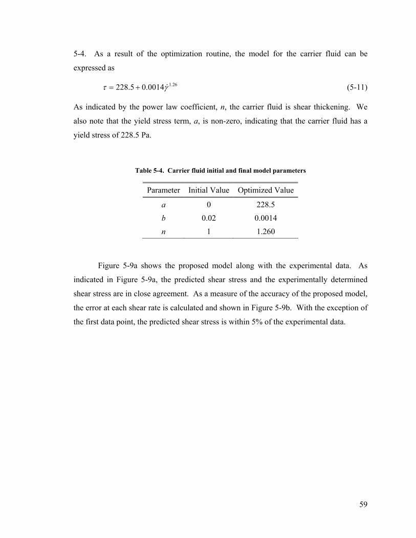
59
5-4. As a result of the optimization routine, the model for the carrier fluid can be
expressed as
26.10014.05.228 γτ &+= (5-11)
As indicated by the power law coefficient, n, the carrier fluid is shear thickening. We
also note that the yield stress term, a, is non-zero, indicating that the carrier fluid has a
yield stress of 228.5 Pa.
Table 5-4. Carrier fluid initial and final model parameters
Parameter Initial Value Optimized Value
a 0 228.5
b 0.02 0.0014
n 1 1.260
Figure 5-9a shows the proposed model along with the experimental data. As
indicated in Figure 5-9a, the predicted shear stress and the experimentally determined
shear stress are in close agreement. As a measure of the accuracy of the proposed model,
the error at each shear rate is calculated and shown in Figure 5-9b. With the exception of
the first data point, the predicted shear stress is within 5% of the experimental data.

60
0 0.5 1 1.5 2 2.5
x 105
-20
-15
-10
-5
0
5
Shear Rate (1/s)
Mod
el E
rror %
0 0.5 1 1.5 2 2.5
x 105
0
1
2
3
4
5
6
7
8
Shear Rate (1/s)
She
ar S
tress
(kP
a)
Experimental DataProposed Model
(a)
(b)
0 0.5 1 1.5 2 2.5
x 105
-20
-15
-10
-5
0
5
Shear Rate (1/s)
Mod
el E
rror %
0 0.5 1 1.5 2 2.5
x 105
0
1
2
3
4
5
6
7
8
Shear Rate (1/s)
She
ar S
tress
(kP
a)
Experimental DataProposed Model
(a)
(b)
Figure 5-9. Carrier fluid model results: (a) Proposed model and experimental data; (b) model error
5.5.2 Proposed model for MR fluid
The optimization routine was run using the MR fluid data. The initial model parameters
and the optimally tuned model parameters are shown in Table 5-5. The resulting model
can be expressed by
053.10727.02.579 γτ &+= (5-12)
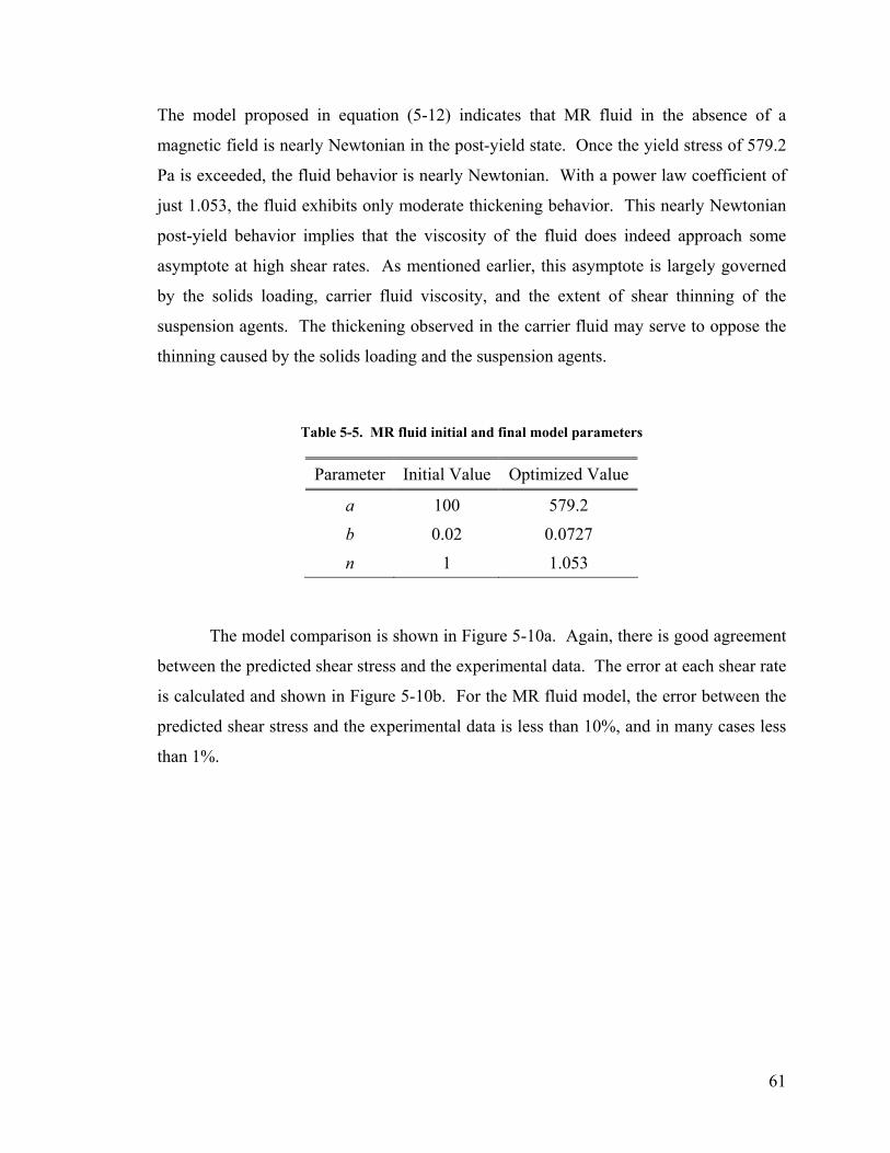
61
The model proposed in equation (5-12) indicates that MR fluid in the absence of a
magnetic field is nearly Newtonian in the post-yield state. Once the yield stress of 579.2
Pa is exceeded, the fluid behavior is nearly Newtonian. With a power law coefficient of
just 1.053, the fluid exhibits only moderate thickening behavior. This nearly Newtonian
post-yield behavior implies that the viscosity of the fluid does indeed approach some
asymptote at high shear rates. As mentioned earlier, this asymptote is largely governed
by the solids loading, carrier fluid viscosity, and the extent of shear thinning of the
suspension agents. The thickening observed in the carrier fluid may serve to oppose the
thinning caused by the solids loading and the suspension agents.
Table 5-5. MR fluid initial and final model parameters
Parameter Initial Value Optimized Value
a 100 579.2
b 0.02 0.0727
n 1 1.053
The model comparison is shown in Figure 5-10a. Again, there is good agreement
between the predicted shear stress and the experimental data. The error at each shear rate
is calculated and shown in Figure 5-10b. For the MR fluid model, the error between the
predicted shear stress and the experimental data is less than 10%, and in many cases less
than 1%.
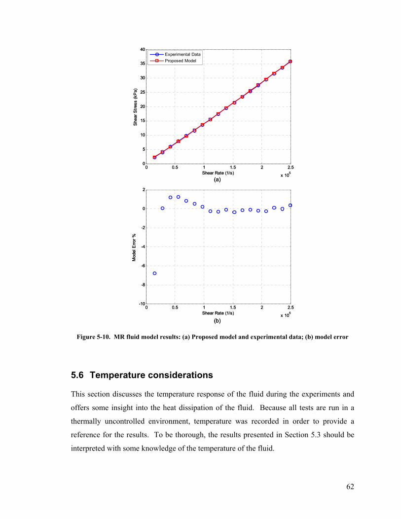
62
0 0.5 1 1.5 2 2.5
x 105
0
5
10
15
20
25
30
35
40
Shear Rate (1/s)
She
ar S
tress
(kP
a)
Experimental DataProposed Model
(a)
(b)
0 0.5 1 1.5 2 2.5
x 105
-10
-8
-6
-4
-2
0
2
Shear Rate (1/s)
Mod
el E
rror %
0 0.5 1 1.5 2 2.5
x 105
0
5
10
15
20
25
30
35
40
Shear Rate (1/s)
She
ar S
tress
(kP
a)
Experimental DataProposed Model
(a)
(b)
0 0.5 1 1.5 2 2.5
x 105
-10
-8
-6
-4
-2
0
2
Shear Rate (1/s)
Mod
el E
rror %
Figure 5-10. MR fluid model results: (a) Proposed model and experimental data; (b) model error
5.6 Temperature considerations
This section discusses the temperature response of the fluid during the experiments and
offers some insight into the heat dissipation of the fluid. Because all tests are run in a
thermally uncontrolled environment, temperature was recorded in order to provide a
reference for the results. To be thorough, the results presented in Section 5.3 should be
interpreted with some knowledge of the temperature of the fluid.
63
Tests were performed at room temperature, though slight fluctuations in room
temperature were observed between experiments. In order to document the temperature
response of the fluid, a thermocouple was placed at the exit of the rheometer. The
temperature response of the carrier fluid is shown in Figure 5-11a. Temperature reaches
steady-state after just 10 mm of stroke. For large piston velocities, i.e. 28 mm/s, a
temperature rise as large as 4 °C can be observed. In Figure 5-11b we note the increase
in steady-state temperature as fluid velocity increases. Furthermore, we note the gradual
increase in the initial fluid temperature. This gradual increase in initial fluid temperature
can be explained if we consider the rate at which mechanical energy is being dissipated.
At a piston velocity of 28 mm/s the corresponding force is 12 kN. The amount of
mechanical power that is being dissipated as heat at this piston velocity is nearly 340
Watts. This dissipation will tend to heat up the fluid as well as the rheometer. As such,
as testing progressed from low piston velocities to high piston velocities, the initial
temperature of the fluid increased slightly.
64
0 5 10 15 20 25 3023
24
25
26
27
28
29
30
Piston Velocity (mm/s)
Exi
t Tem
pera
ture
(o C)
Initial TemperatureFinal Temperature
T∆
(a)
(b)
-10 0 10 20 30 40 50 60 70 80 9023
24
25
26
27
28
29
30
Position (mm)
Tem
pera
ture
(o C)
4 mm/s
8 mm/s
12 mm/s
16 mm/s
20 mm/s
24 mm/s
28 mm/s
0 5 10 15 20 25 3023
24
25
26
27
28
29
30
Piston Velocity (mm/s)
Exi
t Tem
pera
ture
(o C)
Initial TemperatureFinal Temperature
T∆
(a)
(b)
-10 0 10 20 30 40 50 60 70 80 9023
24
25
26
27
28
29
30
Position (mm)
Tem
pera
ture
(o C)
4 mm/s
8 mm/s
12 mm/s
16 mm/s
20 mm/s
24 mm/s
28 mm/s
Figure 5-11. Carrier fluid temperature response: (a) fluid exit temperature over piston stroke; (b)
fluid initial temperature and final temperature as a function of piston velocity
Similar behavior is observed for the MR fluid. The average initial fluid
temperature was 25.8 °C. Figure 5-12a illustrates the temperature response of the MR
fluid as it is driven through the rheometer. At a piston velocity of 36 mm/s, a
temperature increase of nearly 12 °C is observed. In general, a significantly larger
temperature rise is observed for the MR fluid when compared to the carrier fluid. This
behavior can be attributed to the difference in fluid densities; the MR fluid’s density is
3.06 g/cm3, while the carrier fluid density is quite lower at 0.8192 g/cm3. Therefore, the

65
shear heating observed in the MR fluid is dramatically higher. Nearly 2400 Watts of
power are being dissipated at a piston velocity of 36 mm/s. This dissipation tends to heat
both the fluid and the rheometer. Figure 5-12b shows the mean temperature increase for
each velocity. The initial fluid temperature is also shown. A gradual increase in the
initial fluid temperature is observed as the testing progressed from low velocities to high
velocities. This increase in initial fluid temperature would likely be accompanied by an
increase in the temperature of the steel rheometer.
0 5 10 15 20 25 30 35 4024
26
28
30
32
34
36
38
40
Piston Velocity (mm/s)
Exi
t Tem
pera
ture
(o C)
Initial TemperatureFinal Temperature
(a)
(b)
0 20 40 60 80 100 120 14024
26
28
30
32
34
36
38
40
Position (mm)
Tem
pera
ture
(o C)
6 mm/s10 mm/s
16 mm/s
20 mm/s
24 mm/s
30 mm/s
36 mm/s
T∆
0 5 10 15 20 25 30 35 4024
26
28
30
32
34
36
38
40
Piston Velocity (mm/s)
Exi
t Tem
pera
ture
(o C)
Initial TemperatureFinal Temperature
(a)
(b)
0 20 40 60 80 100 120 14024
26
28
30
32
34
36
38
40
Position (mm)
Tem
pera
ture
(o C)
6 mm/s10 mm/s
16 mm/s
20 mm/s
24 mm/s
30 mm/s
36 mm/s
T∆
Figure 5-12. MR fluid temperature response: (a) fluid exit temperature over piston stroke; (b) fluid
initial temperature and final temperature as a function of piston velocity

66
5.7 Summary of off-state behavior
The behavior of MR fluid in the absence of a magnetic field has been the focus of this
chapter. Equally important as the on-state behavior, the off-state behavior of the fluid is
responsible for much of the success attributed to the fluid. Of particular interest in this
study was the high shear behavior of the fluid. Because much of the literature has
suggested that the high shear behavior is largely governed by the carrier fluid, a
characterization of the carrier fluid is also important. Both the carrier fluid and the MR
fluid were run through the high shear rheometer. Shear rates ranged from 0.14x10⁵ s-1 to
2.5x10⁵ s-1. Results for the carrier fluid indicate a considerable shear thickening with a
power law coefficient of 1.26. The MR fluid exhibited nearly Newtonian post-yield
behavior with a power law coefficient of just 1.053. A summary of the proposed models
is given in Table 5-6. Among the range of shear rates considered, the carrier fluid and
the MR fluid had mean viscosities of 0.03 Pa-s and 0.142 Pa-s, respectively.
Table 5-6. Summary of proposed models
Fluid Proposed Model
Carrier 26.10014.05.228 γτ &+=
MR 053.10727.02.579 γτ &+=

67
6 The MR Effect at High Velocities
Perhaps the most compelling feature of MR fluids is their ability to provide high dynamic
yield stresses nearly instantaneously. While the response time of the fluid has yet to be
thoroughly investigated, it is known that the fluid can respond to changes in magnetic
field strength in a matter of milliseconds. This fluid response can be described as a
change in the rheological behavior of the fluid, i.e., the development of a yield stress.
The development of a yield stress upon the application of a magnetic field is commonly
referred to as the MR effect. The degree of MR effect achieved by the fluid is a function
of magnetic field strength. However, because fluid response time is finite, the ability of
the fluid to realize the expected MR effect may be compromised if the fluid does not
spend a sufficient amount of time in the presence of the magnetic field. We define this
time as the dwell time, that is, the amount of time the fluid spends in the presence of a
magnetic field.
It is the intent of this chapter to investigate the MR effect under extreme flow
conditions. The high velocity rheometer discussed in Chapter 4 is used to study the
behavior of the MR fluid at high flow velocities with a magnetic field applied. The
magnetic field is applied over a portion of the flow channel. Dwell time is calculated
from the length of the MR valve and the fluid velocity through the valve. Two MR valve
lengths are considered (25.4 mm and 6.35 mm). Fluid velocities through the valve range
from 1 m/s to 37 m/s with corresponding dwell times ranging from 12.4 ms to 0.18 ms.
The degree of response achieved by the fluid is studied by calculating the yield stress at
each velocity. A significant reduction in the yield stress is observed for dwell times less
than 1 ms.
The organization of the chapter begins with a discussion of the MR effect and
how it is created in MR devices. A discussion of some of the design considerations for
MR valves then follows. Such design considerations include the dwell time of the fluid.
After defining the dwell time, the method of experimentally determining the yield stress
is introduced. The results from the magnetic field testing are presented and the yield
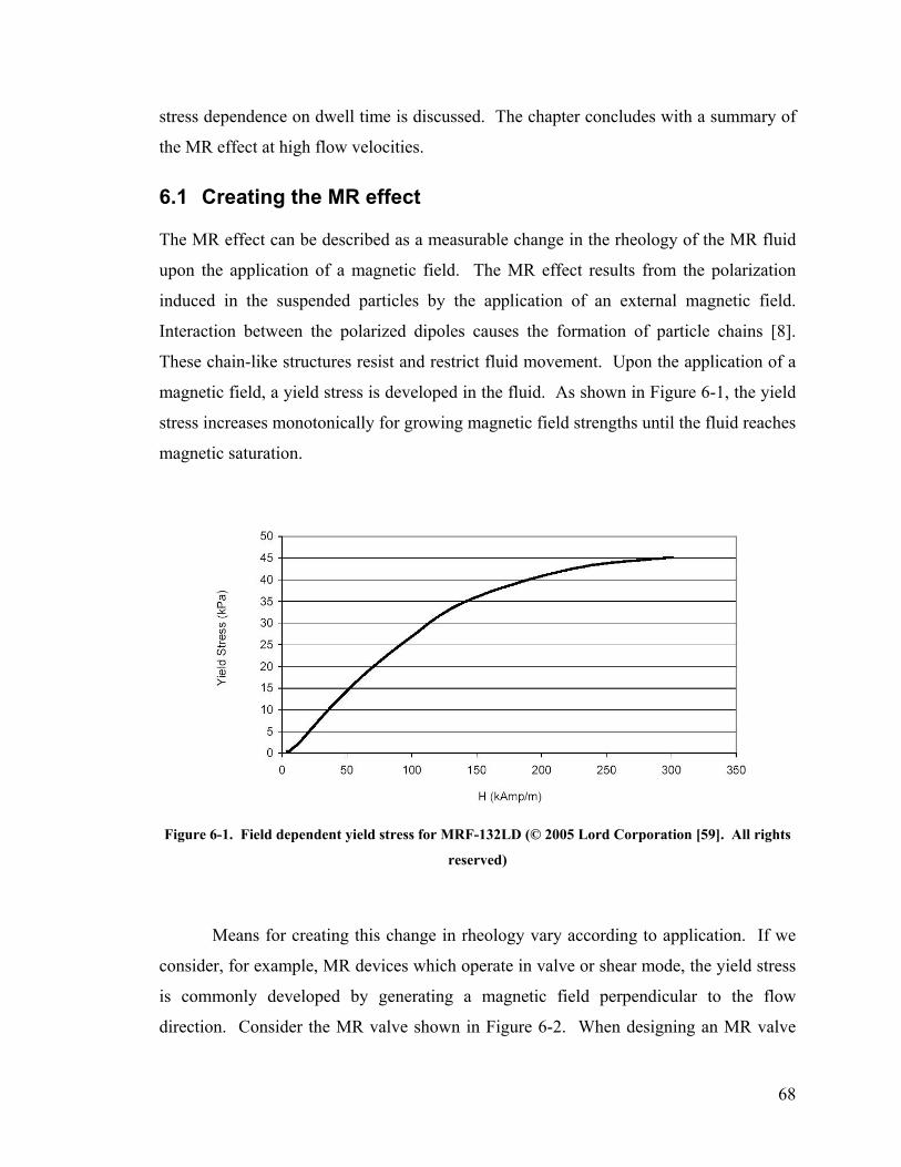
68
stress dependence on dwell time is discussed. The chapter concludes with a summary of
the MR effect at high flow velocities.
6.1 Creating the MR effect
The MR effect can be described as a measurable change in the rheology of the MR fluid
upon the application of a magnetic field. The MR effect results from the polarization
induced in the suspended particles by the application of an external magnetic field.
Interaction between the polarized dipoles causes the formation of particle chains [8].
These chain-like structures resist and restrict fluid movement. Upon the application of a
magnetic field, a yield stress is developed in the fluid. As shown in Figure 6-1, the yield
stress increases monotonically for growing magnetic field strengths until the fluid reaches
magnetic saturation.
Figure 6-1. Field dependent yield stress for MRF-132LD (© 2005 Lord Corporation [59]. All rights
reserved)
Means for creating this change in rheology vary according to application. If we
consider, for example, MR devices which operate in valve or shear mode, the yield stress
is commonly developed by generating a magnetic field perpendicular to the flow
direction. Consider the MR valve shown in Figure 6-2. When designing an MR valve
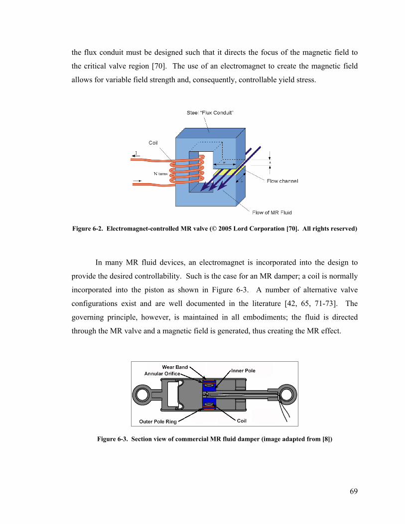
69
the flux conduit must be designed such that it directs the focus of the magnetic field to
the critical valve region [70]. The use of an electromagnet to create the magnetic field
allows for variable field strength and, consequently, controllable yield stress.
Figure 6-2. Electromagnet-controlled MR valve (© 2005 Lord Corporation [70]. All rights reserved)
In many MR fluid devices, an electromagnet is incorporated into the design to
provide the desired controllability. Such is the case for an MR damper; a coil is normally
incorporated into the piston as shown in Figure 6-3. A number of alternative valve
configurations exist and are well documented in the literature [42, 65, 71-73]. The
governing principle, however, is maintained in all embodiments; the fluid is directed
through the MR valve and a magnetic field is generated, thus creating the MR effect.
Figure 6-3. Section view of commercial MR fluid damper (image adapted from [8])
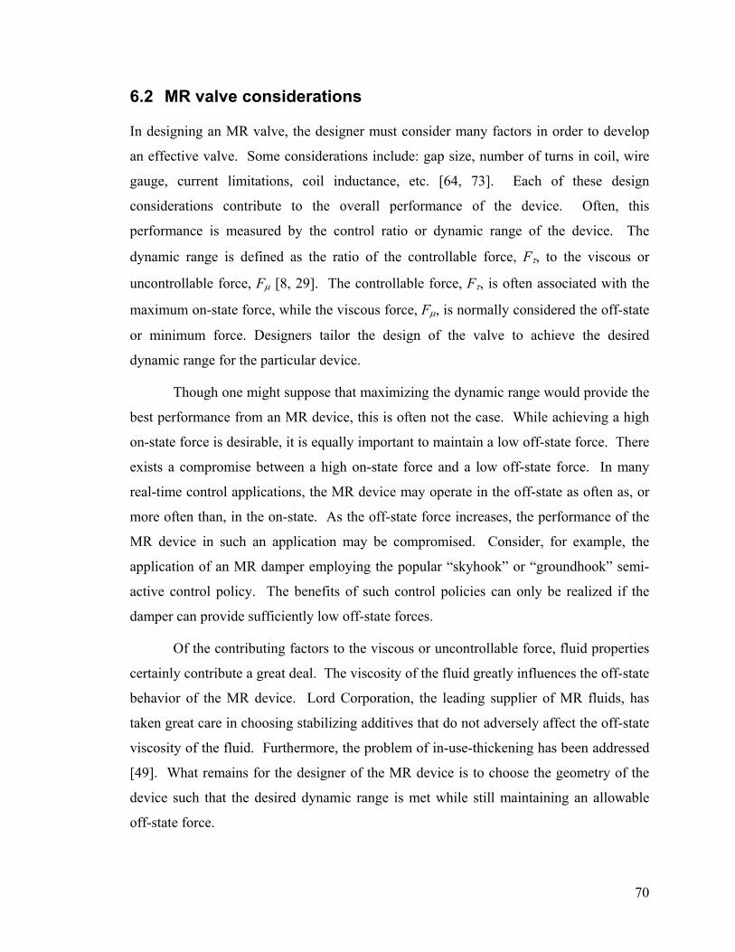
70
6.2 MR valve considerations
In designing an MR valve, the designer must consider many factors in order to develop
an effective valve. Some considerations include: gap size, number of turns in coil, wire
gauge, current limitations, coil inductance, etc. [64, 73]. Each of these design
considerations contribute to the overall performance of the device. Often, this
performance is measured by the control ratio or dynamic range of the device. The
dynamic range is defined as the ratio of the controllable force, Fτ, to the viscous or
uncontrollable force, Fµ [8, 29]. The controllable force, Fτ, is often associated with the
maximum on-state force, while the viscous force, Fµ, is normally considered the off-state
or minimum force. Designers tailor the design of the valve to achieve the desired
dynamic range for the particular device.
Though one might suppose that maximizing the dynamic range would provide the
best performance from an MR device, this is often not the case. While achieving a high
on-state force is desirable, it is equally important to maintain a low off-state force. There
exists a compromise between a high on-state force and a low off-state force. In many
real-time control applications, the MR device may operate in the off-state as often as, or
more often than, in the on-state. As the off-state force increases, the performance of the
MR device in such an application may be compromised. Consider, for example, the
application of an MR damper employing the popular “skyhook” or “groundhook” semi-
active control policy. The benefits of such control policies can only be realized if the
damper can provide sufficiently low off-state forces.
Of the contributing factors to the viscous or uncontrollable force, fluid properties
certainly contribute a great deal. The viscosity of the fluid greatly influences the off-state
behavior of the MR device. Lord Corporation, the leading supplier of MR fluids, has
taken great care in choosing stabilizing additives that do not adversely affect the off-state
viscosity of the fluid. Furthermore, the problem of in-use-thickening has been addressed
[49]. What remains for the designer of the MR device is to choose the geometry of the
device such that the desired dynamic range is met while still maintaining an allowable
off-state force.
71
The means by which a designer can achieve the desired dynamic range and low
off-state force are well demonstrated if we consider the design of an MR valve for an MR
damper. Recall the MR damper shown in Figure 6-3. The force generated by the MR
damper can be separated into two components: the viscous or off-state force, Fµ, and the
field induced controllable force, Fmr. Using the parallel plate approximation, these forces
can be approximated by [29]
3
122
1wh
LQAQ
whvF po µµ
+= (6-1)
hLA
cF pomr
τ= (6-2)
where L, w, and h are the length, width, and gap of the flow channel, µ is the off-state
viscosity, Q is the flow rate, τo is the field dependent yield stress, vo is the pole velocity,
and Ap is the area of the piston. The coefficient c is a function of the flow velocity profile
and is normally taken to be between 2 and 3 [8]. Equation (6-1) illustrates the dominant
effect of the gap size on off-state force. Because the fluid gap is cubed in equation (6-1),
the off-state force is highly sensitive to changes in the fluid gap size. The field dependent
controllable force is less sensitive to changes in the fluid gap. Because the two forces, Fµ
and Fmr, are not equally sensitive to changes in gap size, the gap size often becomes a key
design element.
The gap size is often chosen to achieve the desired off-state force. A larger gap
size will reduce the viscous or uncontrollable force of the damper. As a consequence,
however, the maximum on-state or controllable force is also reduced. The designer can
then turn to alternative measures for increasing the maximum controllable force. In order
to compensate for the larger gap size, MR dampers often employ multi-stage MR valves.
Consider the axisymmetric MR valves shown in Figure 6-4. Figure 6-4a shows a single
stage MR valve, commonly found in MR dampers such as the MotionMasterTM damper
[8]. A single stage MR valve contains a single coil which creates the “choking regions”
responsible for the controllable force. With the addition of a second coil, a two-stage MR
valve, as shown in Figure 6-4b, has twice the number of choking regions. The coils are
alternately-wound such that the magnetic fields are additive and do not cancel each other

72
[65, 73]. With the additional choking regions, a two-stage valve can provide a greater
level of on-state force. Lord Corporation’s 180 kN seismic damper [65], shown in Figure
6-4c, employs a 3-stage piston to generate the desired on-state force. Multi-stage pistons
allow designers to compensate for larger gap sizes with added controllability from
additional activation regions. By increasing the number of activation regions, the active
fluid volume increases accordingly. It has been shown that the active fluid volume
contributes directly to the dynamic range of the device [8, 52, 71, 72].
(a)
(b)
(c)
MR Valve Length
L1 L2 L3
Lmr = L1 + L2 + L3
2mrL
2mrL
pL
(a)
(b)
(c)
MR Valve Length
L1 L2 L3
Lmr = L1 + L2 + L3
MR Valve Length
L1 L2 L3
Lmr = L1 + L2 + L3
2mrL
2mrL
pL
2mrL
2mrL
pL
Figure 6-4. Axisymmetric MR valves: (a) single-stage piston (image adapted from [70]); (b) dual-
stage piston (image adapted from [73]); (c) 3-stage piston (© 2005 Lord Corporation [4]. All rights
reserved)

73
From the MR valve configurations shown in Figure 6-4, we can identify passive
and active portions of the MR valve. As shown in Figure 6-4a, the entire valve length is
not activated; the portion of the valve which contains the coil is inactive. We define the
active valve length as the portion of the MR valve which acts upon the MR fluid. The
active length, or magnetic pole length, of the piston shown in Figure 6-4b, for example, is
3.3 cm out of a total piston length of 4.0 cm [73]. Likewise, for the 3-stage piston in
Figure 6-4c, the effective pole length is 8.4 cm, with a total piston length of 22.4 cm [29,
65]. This portion of the MR valve is responsible for the rheological change in the fluid,
i.e., the MR effect. The active length of the MR valve becomes a matter of significant
importance in applications in which the fluid is operating under extreme flow conditions.
6.3 Fluid dwell time
As the fluid flows through the MR valve, it is subjected to a magnetic field in the active
valve regions. Over this portion of MR valve, the fluid develops its yield stress and
allows for controllability in the force. As the fluid enters the active valve region, the
transition from Newtonian-like flow to Bingham plastic flow occurs. Though it is known
that MR fluid response to a magnetic field occurs in a matter of milliseconds [2, 3], the
degree of response achieved by the fluid has yet to be addressed.
We confront this issue by first defining the fluid dwell time, also referred to as
residence time as described in the work by Bullough et al. [74]. Dwell time is defined as
the amount of time the fluid spends in the presence of a magnetic field. In other words,
dwell time is the time it takes the fluid to flow through the MR valve. Dwell time is
calculated from
m
mrdwell u
Lt = (6-3)
where Lmr is the length of the MR valve and um is the mean fluid velocity through the
flow channel. Consider, as an example, an extreme case in which the fluid is stationary
in an active region of an MR valve. In such a case, the fluid will develop its full
potential, or 100% of its expected yield stress with the application of a magnetic field.
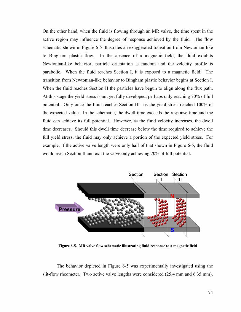
74
On the other hand, when the fluid is flowing through an MR valve, the time spent in the
active region may influence the degree of response achieved by the fluid. The flow
schematic shown in Figure 6-5 illustrates an exaggerated transition from Newtonian-like
to Bingham plastic flow. In the absence of a magnetic field, the fluid exhibits
Newtonian-like behavior; particle orientation is random and the velocity profile is
parabolic. When the fluid reaches Section I, it is exposed to a magnetic field. The
transition from Newtonian-like behavior to Bingham plastic behavior begins at Section I.
When the fluid reaches Section II the particles have begun to align along the flux path.
At this stage the yield stress is not yet fully developed, perhaps only reaching 70% of full
potential. Only once the fluid reaches Section III has the yield stress reached 100% of
the expected value. In the schematic, the dwell time exceeds the response time and the
fluid can achieve its full potential. However, as the fluid velocity increases, the dwell
time decreases. Should this dwell time decrease below the time required to achieve the
full yield stress, the fluid may only achieve a portion of the expected yield stress. For
example, if the active valve length were only half of that shown in Figure 6-5, the fluid
would reach Section II and exit the valve only achieving 70% of full potential.
S
N
SectionIII
SectionII
SectionI
Pressure
S
N
SectionIII
SectionII
SectionI
Pressure
Figure 6-5. MR valve flow schematic illustrating fluid response to a magnetic field
The behavior depicted in Figure 6-5 was experimentally investigated using the
slit-flow rheometer. Two active valve lengths were considered (25.4 mm and 6.35 mm).

75
Fluid velocities ranged from 1 m/s to 37 m/s with corresponding dwell times ranging
from 12.4 ms to 0.18 ms. Figure 6-6 shows the dwell time as a function of fluid velocity
for each valve length. With the 25.4 mm valve length, dwell times were between 12.4 ms
and 0.69 ms, while for the 6.35 mm valve length, dwell times dropped to between 6.4 ms
and 0.18 ms. For the 6.35 mm valve length, the piston velocities were chosen such that
there was a large concentration of dwell times close to 1 ms. This was done in order to
highlight the response of the fluid at dwell times close to 1 ms. The yield stress was
found from the measured force for each fluid velocity and evaluated as a function of the
dwell time.
0 5 10 15 20 25 30 35 400
1
2
3
4
5
6
7
8
9
10
11
12
13
14
Fluid Velocity (m/s)
Dw
ell T
ime
(ms)
Lmr = 25.4 mm
Lmr = 6.35 mm
Figure 6-6. Dwell time of fluid through active valve length
6.4 Experimental determination of the yield stress
Recall from the description of the rheometer in Chapter 4 that the flow channel was given
as 101.6 mm with the MR valve incorporated into the last 25.4 mm of the channel.
Figure 6-7 shows the flow channel with the 25.4 mm MR valve. The magnetic field was
applied to the active MR valve portion only. When testing with the 6.35 mm MR valve,
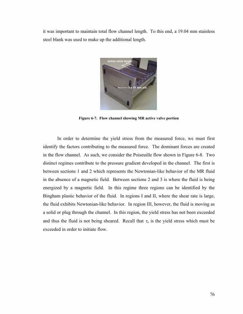
76
it was important to maintain total flow channel length. To this end, a 19.04 mm stainless
steel blank was used to make up the additional length.
active valve length
1 x 10 mm slit
active valve length
1 x 10 mm slit
Figure 6-7. Flow channel showing MR active valve portion
In order to determine the yield stress from the measured force, we must first
identify the factors contributing to the measured force. The dominant forces are created
in the flow channel. As such, we consider the Poiseuille flow shown in Figure 6-8. Two
distinct regimes contribute to the pressure gradient developed in the channel. The first is
between sections 1 and 2 which represents the Newtonian-like behavior of the MR fluid
in the absence of a magnetic field. Between sections 2 and 3 is where the fluid is being
energized by a magnetic field. In this regime three regions can be identified by the
Bingham plastic behavior of the fluid. In regions I and II, where the shear rate is large,
the fluid exhibits Newtonian-like behavior. In region III, however, the fluid is moving as
a solid or plug through the channel. In this region, the yield stress has not been exceeded
and thus the fluid is not being sheared. Recall that τo is the yield stress which must be
exceeded in order to initiate flow.

77
x
up
2 3
Lmr
hb
ha τ
-τo
τo
I
III
II
y
h
u
1
L
τ
N
S x
up
2 3
Lmr
hb
ha τ
-τo
τo
I
III
II
y
h
u
1
L
τ
N
S
Figure 6-8. Flow transition through fixed parallel plates
From the pressure gradient derivation developed in Chapter 3, the pressure in the
flow channel can be written as the sum of the pressure developed in the Newtonian
regime and pressure developed in the non-Newtonian regime, i.e. the MR valve. The
force generated in the flow channel is simply the combined pressure of the Newtonian
regime, Pµ, and the Bingham regime, Pmr, acting over the area of the piston, Ap.
( )mrp PPAF ∆+∆= µ (6-4)
where
( )mrm LL
huP −=∆ 2
12 µµ (6-5)
and
mrm
mr Lhu
P 2
12 µP=∆ (6-6)
In equation (6-5) and equation (6-6), um is the mean fluid velocity through the channel, µ
is the fluid viscosity, and h is the gap size. L and Lmr are the lengths of the flow channel
and the length of the MR valve, respectively. P is the non-dimensional pressure drop
introduced in Chapter 3. Because force is a measured quantity, we can solve equation (6-
4) for the pressure developed in the MR valve
µPAFP
pmr ∆−=∆ (6-6)
78
Substituting equation (6-5) and equation (6-6) into equation (6-7), we have an expression
for the non-dimensional pressure gradient in terms of the measured force
mr
mr
mrmp LLL
Luh
AF −
−=µ12
2
P (6-8)
Recall the cubic equation presented in Chapter 3, repeated here for convenience,
( ) 0431 323 =++− TPTP (6-9)
where P and T are given by
µmuh
dxdp
12
2
−=P (6-10)
µτ
m
o
uh
12=T (6-11)
In equation (6-10), dp/dx is the pressure gradient developed along the MR valve length,
and τo in equation (6-11) is the yield stress. Because P is known from equation (6-8), the
equation of interest becomes the cubic in T
( ) 041
43 2323 =−+− PPTPT (6-12)
Rewriting equation (6-9) in this form, we can solve for the roots of T in terms of P, where
P is found from the measured force. The desired root is given by [56]
( )
+
−
=3
41acos31cos π
PPPPT (6-13)
The yield stress is then found from equation (6-11) as
Thum
oµ
τ12
= (6-14)
It should be noted that the viscosity used in the calculation of the yield stress was
determined from the off-state viscosity discussed in Chapter 5. The shear-thinning
behavior has been accounted for in the yield stress calculations. Furthermore, by using

79
the viscosity obtained in experiments, any variation in temperature that may have existed
between experiments was accounted for.
6.5 Magnetic field testing
The yield stress was found for a number of magnetic field strengths and two active MR
valve lengths. The 25.4 mm valve length was activated with field strengths of 100 kA/m
and 200 kA/m at 18 piston velocities ranging from 2 mm/s to 36 mm/s. Piston velocities
increased at an increment of 2 mm/s. Experiments with the 6.35 mm valve length were
performed at three magnetic field strengths (100 kA/m, 150 kA/m, and 200 kA/m).
Piston velocities for the 6.35 mm valve ranged from 1 mm/s to 35 mm/s. At this valve
length, 10 piston velocities were tested between 1 mm/s and 5 mm/s, and another 5
velocities between 6 mm/s and 10 mm/s. This was done in order to highlight the
response of the fluid at dwell times close to 1 ms. Above piston velocities of 10 mm/s,
the velocity increment increased to 5 mm/s.
Figure 6-9 shows the force versus position for several piston velocities at
magnetic field strengths of 100 kA/m and 200 kA/m for both valve lengths. In Figure 6-9
we note a marked increase in force for the 25.4 mm valve length as the magnetic field
increases from 100 kA/m, Figure 6-9a, to 200 kA/m, Figure 6-9b. The same cannot be
said for the 6.35 mm valve. For large piston velocities the increase in magnetic field
from 100 kA/m, Figure 6-9c, to 200 kA/m, Figure 6-9d, results in only a marginal
increase in force. At low piston velocities, however, there is a noticeable increase in
force for the 6.35 mm valve. We also note, in comparing the forces for each valve
length, that for similar velocities the force achieved with the 6.35 mm active valve length
is significantly less than the force achieved with the 25.4 mm valve length. This is
expected since the active valve length for the 6.35 mm valve is 1/4th of the 25.4 mm
valve. As such, the yield stress is being developed over a shorter portion of the flow
channel. These results are better illustrated if we consider the force, or pressure, as a
function of fluid velocity.
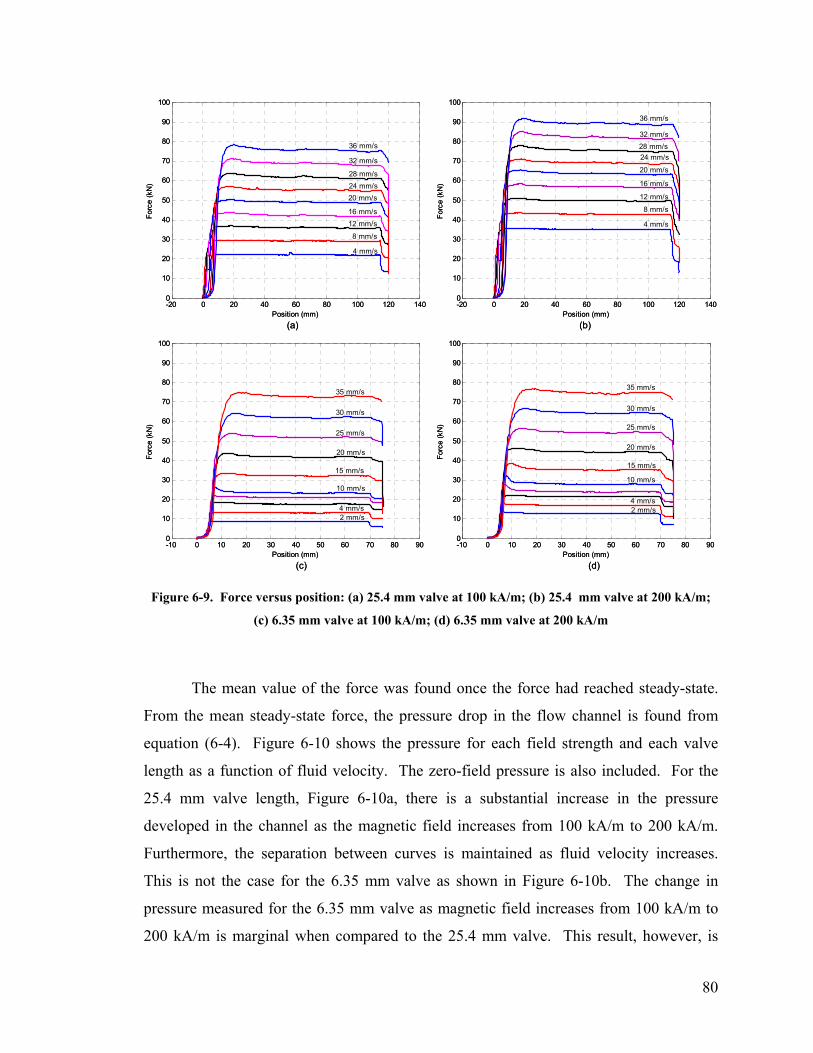
80
-20 0 20 40 60 80 100 120 1400
10
20
30
40
50
60
70
80
90
100
Position (mm)
Forc
e (k
N)
4 mm/s
28 mm/s24 mm/s
20 mm/s
16 mm/s
12 mm/s
8 mm/s
32 mm/s
36 mm/s
(b)
(d)
(a)
(c)
-20 0 20 40 60 80 100 120 1400
10
20
30
40
50
60
70
80
90
100
Position (mm)
Forc
e (k
N)
4 mm/s
8 mm/s
12 mm/s16 mm/s
20 mm/s24 mm/s28 mm/s
32 mm/s
36 mm/s
-10 0 10 20 30 40 50 60 70 80 900
10
20
30
40
50
60
70
80
90
100
Position (mm)
Forc
e (k
N)
2 mm/s
35 mm/s
30 mm/s
25 mm/s
20 mm/s
15 mm/s
10 mm/s
4 mm/s
-10 0 10 20 30 40 50 60 70 80 900
10
20
30
40
50
60
70
80
90
100
Position (mm)
Forc
e (k
N)
2 mm/s4 mm/s
10 mm/s
15 mm/s
20 mm/s
25 mm/s
30 mm/s
35 mm/s
-20 0 20 40 60 80 100 120 1400
10
20
30
40
50
60
70
80
90
100
Position (mm)
Forc
e (k
N)
4 mm/s
28 mm/s24 mm/s
20 mm/s
16 mm/s
12 mm/s
8 mm/s
32 mm/s
36 mm/s
(b)
(d)
(a)
(c)
-20 0 20 40 60 80 100 120 1400
10
20
30
40
50
60
70
80
90
100
Position (mm)
Forc
e (k
N)
4 mm/s
8 mm/s
12 mm/s16 mm/s
20 mm/s24 mm/s28 mm/s
32 mm/s
36 mm/s
-10 0 10 20 30 40 50 60 70 80 900
10
20
30
40
50
60
70
80
90
100
Position (mm)
Forc
e (k
N)
2 mm/s
35 mm/s
30 mm/s
25 mm/s
20 mm/s
15 mm/s
10 mm/s
4 mm/s
-10 0 10 20 30 40 50 60 70 80 900
10
20
30
40
50
60
70
80
90
100
Position (mm)
Forc
e (k
N)
2 mm/s4 mm/s
10 mm/s
15 mm/s
20 mm/s
25 mm/s
30 mm/s
35 mm/s
Figure 6-9. Force versus position: (a) 25.4 mm valve at 100 kA/m; (b) 25.4 mm valve at 200 kA/m;
(c) 6.35 mm valve at 100 kA/m; (d) 6.35 mm valve at 200 kA/m
The mean value of the force was found once the force had reached steady-state.
From the mean steady-state force, the pressure drop in the flow channel is found from
equation (6-4). Figure 6-10 shows the pressure for each field strength and each valve
length as a function of fluid velocity. The zero-field pressure is also included. For the
25.4 mm valve length, Figure 6-10a, there is a substantial increase in the pressure
developed in the channel as the magnetic field increases from 100 kA/m to 200 kA/m.
Furthermore, the separation between curves is maintained as fluid velocity increases.
This is not the case for the 6.35 mm valve as shown in Figure 6-10b. The change in
pressure measured for the 6.35 mm valve as magnetic field increases from 100 kA/m to
200 kA/m is marginal when compared to the 25.4 mm valve. This result, however, is

81
expected due to the dramatic reduction in the active valve length. The significance of the
result shown in Figure 6-10b is the behavior observed as the fluid velocity increases. For
low fluid velocities the pressure differential between field strengths is maintained.
However, as the fluid velocity continues to grow the pressure differential decreases;
pressures for the 100 kA/m, 150 kA/m, and 200 kA/m tests appear to converge towards
the zero-field case. This implies that, with the 6.35 mm active valve length, the yield
stress being developed in the fluid is not being maintained as fluid velocity increases.
(a)
(b)
0 5 10 15 20 25 30 35 400
2
4
6
8
10
12
Fluid Velocity (m/s)
Pre
ssur
e (M
Pa)
f0 = 0 kA/mf1 = 100 kA/mf2 = 200 kA/m
0 5 10 15 20 25 30 35 400
2
4
6
8
10
12
Fluid Velocity (m/s)
Pre
ssur
e (M
Pa)
f0 = 0 kA/mf1 = 100 kA/mf2 = 150 kA/mf3 = 200 kA/m
(a)
(b)
0 5 10 15 20 25 30 35 400
2
4
6
8
10
12
Fluid Velocity (m/s)
Pre
ssur
e (M
Pa)
f0 = 0 kA/mf1 = 100 kA/mf2 = 200 kA/m
0 5 10 15 20 25 30 35 400
2
4
6
8
10
12
Fluid Velocity (m/s)
Pre
ssur
e (M
Pa)
f0 = 0 kA/mf1 = 100 kA/mf2 = 150 kA/mf3 = 200 kA/m
Figure 6-10. Pressure in flow channel as a function of fluid velocity: (a) 25.4 mm valve; (b) 6.35 mm
valve
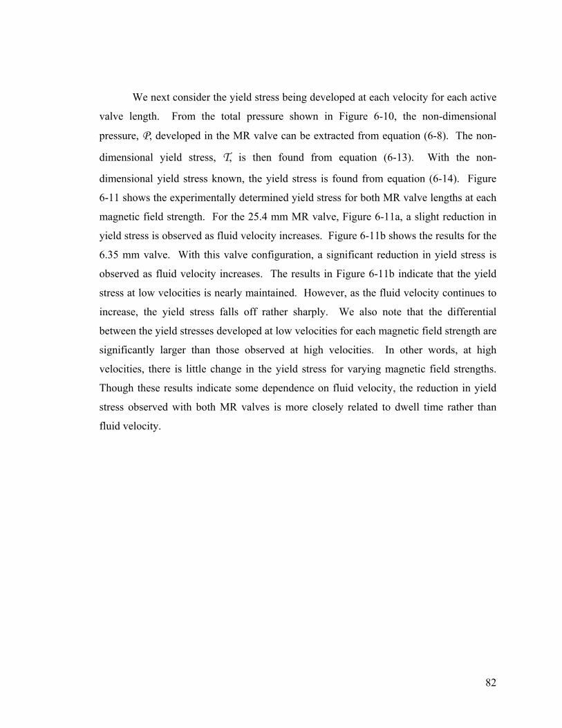
82
We next consider the yield stress being developed at each velocity for each active
valve length. From the total pressure shown in Figure 6-10, the non-dimensional
pressure, P, developed in the MR valve can be extracted from equation (6-8). The non-
dimensional yield stress, T, is then found from equation (6-13). With the non-
dimensional yield stress known, the yield stress is found from equation (6-14). Figure
6-11 shows the experimentally determined yield stress for both MR valve lengths at each
magnetic field strength. For the 25.4 mm MR valve, Figure 6-11a, a slight reduction in
yield stress is observed as fluid velocity increases. Figure 6-11b shows the results for the
6.35 mm valve. With this valve configuration, a significant reduction in yield stress is
observed as fluid velocity increases. The results in Figure 6-11b indicate that the yield
stress at low velocities is nearly maintained. However, as the fluid velocity continues to
increase, the yield stress falls off rather sharply. We also note that the differential
between the yield stresses developed at low velocities for each magnetic field strength are
significantly larger than those observed at high velocities. In other words, at high
velocities, there is little change in the yield stress for varying magnetic field strengths.
Though these results indicate some dependence on fluid velocity, the reduction in yield
stress observed with both MR valves is more closely related to dwell time rather than
fluid velocity.
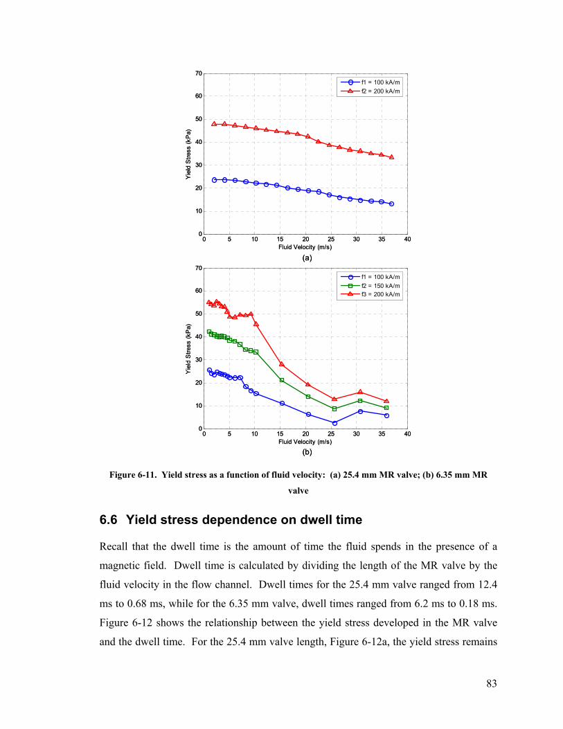
83
(a)
(b)
0 5 10 15 20 25 30 35 400
10
20
30
40
50
60
70
Fluid Velocity (m/s)
Yie
ld S
tress
(kP
a)
f1 = 100 kA/mf2 = 200 kA/m
0 5 10 15 20 25 30 35 400
10
20
30
40
50
60
70
Fluid Velocity (m/s)
Yie
ld S
tress
(kP
a)
f1 = 100 kA/mf2 = 150 kA/mf3 = 200 kA/m
(a)
(b)
0 5 10 15 20 25 30 35 400
10
20
30
40
50
60
70
Fluid Velocity (m/s)
Yie
ld S
tress
(kP
a)
f1 = 100 kA/mf2 = 200 kA/m
0 5 10 15 20 25 30 35 400
10
20
30
40
50
60
70
Fluid Velocity (m/s)
Yie
ld S
tress
(kP
a)
f1 = 100 kA/mf2 = 150 kA/mf3 = 200 kA/m
Figure 6-11. Yield stress as a function of fluid velocity: (a) 25.4 mm MR valve; (b) 6.35 mm MR
valve
6.6 Yield stress dependence on dwell time
Recall that the dwell time is the amount of time the fluid spends in the presence of a
magnetic field. Dwell time is calculated by dividing the length of the MR valve by the
fluid velocity in the flow channel. Dwell times for the 25.4 mm valve ranged from 12.4
ms to 0.68 ms, while for the 6.35 mm valve, dwell times ranged from 6.2 ms to 0.18 ms.
Figure 6-12 shows the relationship between the yield stress developed in the MR valve
and the dwell time. For the 25.4 mm valve length, Figure 6-12a, the yield stress remains
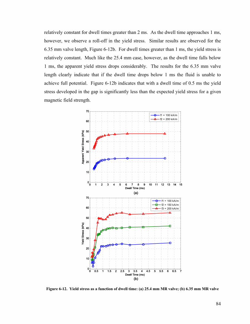
84
relatively constant for dwell times greater than 2 ms. As the dwell time approaches 1 ms,
however, we observe a roll-off in the yield stress. Similar results are observed for the
6.35 mm valve length, Figure 6-12b. For dwell times greater than 1 ms, the yield stress is
relatively constant. Much like the 25.4 mm case, however, as the dwell time falls below
1 ms, the apparent yield stress drops considerably. The results for the 6.35 mm valve
length clearly indicate that if the dwell time drops below 1 ms the fluid is unable to
achieve full potential. Figure 6-12b indicates that with a dwell time of 0.5 ms the yield
stress developed in the gap is significantly less than the expected yield stress for a given
magnetic field strength.
(a)
(b)
0 1 2 3 4 5 6 7 8 9 10 11 12 13 14 150
10
20
30
40
50
60
70
Dwell Time (ms)
App
aren
t Yie
ld S
tress
(kP
a)
f1 = 100 kA/mf2 = 200 kA/m
0 0.5 1 1.5 2 2.5 3 3.5 4 4.5 5 5.5 6 6.5 70
10
20
30
40
50
60
70
Dwell Time (ms)
Yie
ld S
tress
(kP
a)
f1 = 100 kA/mf2 = 150 kA/mf3 = 200 kA/m
(a)
(b)
0 1 2 3 4 5 6 7 8 9 10 11 12 13 14 150
10
20
30
40
50
60
70
Dwell Time (ms)
App
aren
t Yie
ld S
tress
(kP
a)
f1 = 100 kA/mf2 = 200 kA/m
0 0.5 1 1.5 2 2.5 3 3.5 4 4.5 5 5.5 6 6.5 70
10
20
30
40
50
60
70
Dwell Time (ms)
Yie
ld S
tress
(kP
a)
f1 = 100 kA/mf2 = 150 kA/mf3 = 200 kA/m
Figure 6-12. Yield stress as a function of dwell time: (a) 25.4 mm MR valve; (b) 6.35 mm MR valve

85
As a measure of the degree of response achieved by the fluid, we normalize the
yield stress with respect to the maximum yield stress observed for each field strength as
( )o
o
ττ
max=Ψ (6-15)
Figure 6-13 shows the normalized yield stress as a function of dwell time. In this
representation, we observe that for the 25.4 mm MR valve, Figure 6-13a, the fluid is still
able to achieve greater than 50% of the maximum yield stress for dwell times as low as
0.68 ms. As the dwell time decreases further below 1 ms, however, as in the 6.35 mm
valve length, Figure 6-13b shows that the yield stress is reduced to as little as 10% of the
maximum value.
The results in Figure 6-13 also indicate that a higher magnetic field can “delay”
the reduction of the yield stress. Figure 6-13a shows that the yield stress for the 100
kA/m magnetic field strength begins to falls sooner than the 200 kA/m field strength.
The normalized yield stress is consistently higher for the 200 kA/m field strength than for
the 100 kA/m field strength. If we consider, for example, the value of the normalized
yield stress at 0.68 ms, we see that the 200 kA/m field strength is achieving 70% of the
maximum value while the 100 kA/m field strength has already fallen to 55%. The same
can be said for the 6.35 mm valve length. From Figure 6-13b, we see that the normalized
yield stress for the 100 kA/m field strength drops sooner and more dramatically than the
other two magnetic field strengths.
86
(a)
(b)
0 1 2 3 4 5 6 7 8 9 10 11 12 13 14 150
0.1
0.2
0.3
0.4
0.5
0.6
0.7
0.8
0.9
1
Dwell Time (ms)
Nor
mal
ized
Yie
ld S
tress
( τo/ τ
oMA
X)
f1 = 100 kA/mf2 = 200 kA/m
0 0.5 1 1.5 2 2.5 3 3.5 4 4.5 5 5.5 6 6.5 70
0.1
0.2
0.3
0.4
0.5
0.6
0.7
0.8
0.9
1
Dwell Time (ms)
Nor
mal
ized
Yie
ld S
tress
( τo/ τ
oMA
X)
f1 = 100 kA/mf2 = 150 kA/mf3 = 200 kA/m
Figure 6-13. Normalized yield stress as a function of dwell time: (a) 25.4 mm MR valve; (b) 6.35 mm
MR valve
6.7 Modeling the MR effect at high velocities
As a characterization of the MR effect at high velocities, a model based on the
experimental results is proposed. Thus far, the results indicate that the normalized yield
stress is predominantly a function of dwell time. However, as observed in Figure 6-13,
the normalized yield stress is also a function of the magnetic field strength. Consider
Figure 6-14, in which we further generalize the yield stress results, and present the
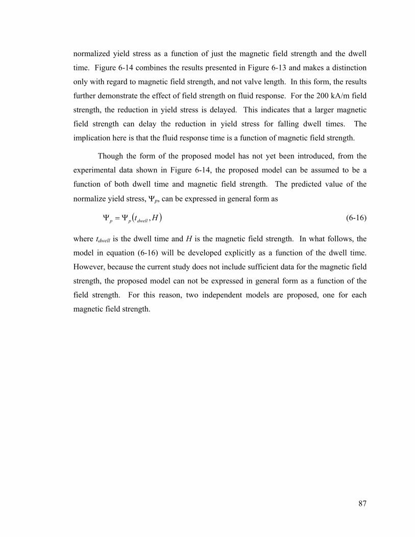
87
normalized yield stress as a function of just the magnetic field strength and the dwell
time. Figure 6-14 combines the results presented in Figure 6-13 and makes a distinction
only with regard to magnetic field strength, and not valve length. In this form, the results
further demonstrate the effect of field strength on fluid response. For the 200 kA/m field
strength, the reduction in yield stress is delayed. This indicates that a larger magnetic
field strength can delay the reduction in yield stress for falling dwell times. The
implication here is that the fluid response time is a function of magnetic field strength.
Though the form of the proposed model has not yet been introduced, from the
experimental data shown in Figure 6-14, the proposed model can be assumed to be a
function of both dwell time and magnetic field strength. The predicted value of the
normalize yield stress, Ψp, can be expressed in general form as
( )Htdwellpp ,Ψ=Ψ (6-16)
where tdwell is the dwell time and H is the magnetic field strength. In what follows, the
model in equation (6-16) will be developed explicitly as a function of the dwell time.
However, because the current study does not include sufficient data for the magnetic field
strength, the proposed model can not be expressed in general form as a function of the
field strength. For this reason, two independent models are proposed, one for each
magnetic field strength.
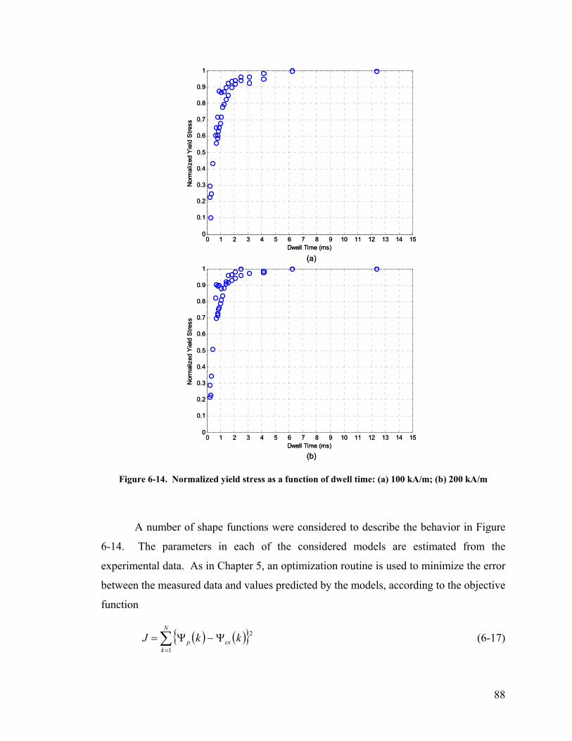
88
(a)
(b)
0 1 2 3 4 5 6 7 8 9 10 11 12 13 14 150
0.1
0.2
0.3
0.4
0.5
0.6
0.7
0.8
0.9
1
Dwell Time (ms)
Nor
mal
ized
Yie
ld S
tress
0 1 2 3 4 5 6 7 8 9 10 11 12 13 14 150
0.1
0.2
0.3
0.4
0.5
0.6
0.7
0.8
0.9
1
Dwell Time (ms)
Nor
mal
ized
Yie
ld S
tress
(a)
(b)
0 1 2 3 4 5 6 7 8 9 10 11 12 13 14 150
0.1
0.2
0.3
0.4
0.5
0.6
0.7
0.8
0.9
1
Dwell Time (ms)
Nor
mal
ized
Yie
ld S
tress
0 1 2 3 4 5 6 7 8 9 10 11 12 13 14 150
0.1
0.2
0.3
0.4
0.5
0.6
0.7
0.8
0.9
1
Dwell Time (ms)
Nor
mal
ized
Yie
ld S
tress
Figure 6-14. Normalized yield stress as a function of dwell time: (a) 100 kA/m; (b) 200 kA/m
A number of shape functions were considered to describe the behavior in Figure
6-14. The parameters in each of the considered models are estimated from the
experimental data. As in Chapter 5, an optimization routine is used to minimize the error
between the measured data and values predicted by the models, according to the objective
function
( ) ( ){ }∑=
Ψ−Ψ=N
kexp kkJ
1
2 (6-17)
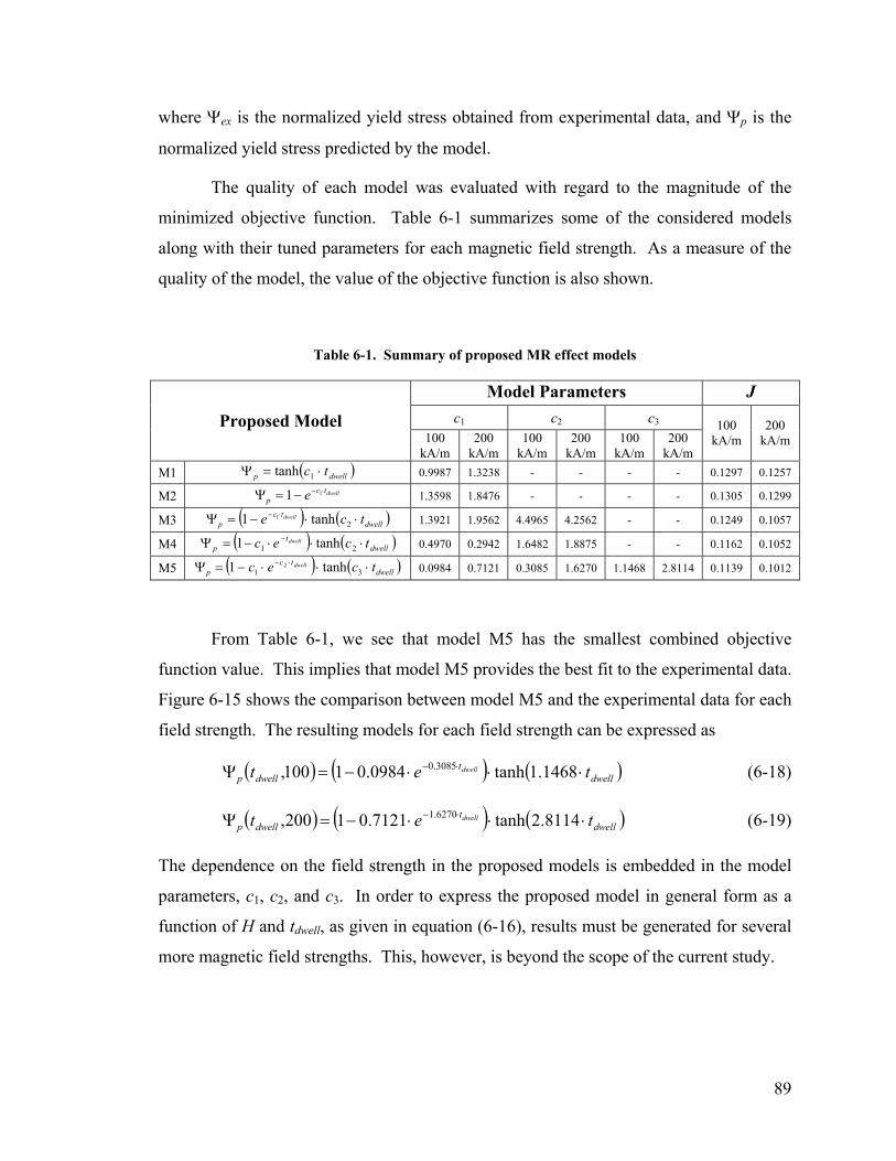
89
where Ψex is the normalized yield stress obtained from experimental data, and Ψp is the
normalized yield stress predicted by the model.
The quality of each model was evaluated with regard to the magnitude of the
minimized objective function. Table 6-1 summarizes some of the considered models
along with their tuned parameters for each magnetic field strength. As a measure of the
quality of the model, the value of the objective function is also shown.
Table 6-1. Summary of proposed MR effect models
Model Parameters J c1 c2 c3 Proposed Model
100 kA/m
200 kA/m
100 kA/m
200 kA/m
100 kA/m
200 kA/m
100 kA/m
200 kA/m
M1 ( )dwellp tc ⋅=Ψ 1tanh 0.9987 1.3238 - - - - 0.1297 0.1257
M2 dwelltcp e ⋅−−=Ψ 11 1.3598 1.8476 - - - - 0.1305 0.1299
M3 ( ) ( )dwelltc
p tce dwell ⋅⋅−=Ψ ⋅−2tanh1 1 1.3921 1.9562 4.4965 4.2562 - - 0.1249 0.1057
M4 ( ) ( )dwellt
p tcec dwell ⋅⋅⋅−=Ψ −21 tanh1 0.4970 0.2942 1.6482 1.8875 - - 0.1162 0.1052
M5 ( ) ( )dwelltc
p tcec dwell ⋅⋅⋅−=Ψ ⋅−31 tanh1 2 0.0984 0.7121 0.3085 1.6270 1.1468 2.8114 0.1139 0.1012
From Table 6-1, we see that model M5 has the smallest combined objective
function value. This implies that model M5 provides the best fit to the experimental data.
Figure 6-15 shows the comparison between model M5 and the experimental data for each
field strength. The resulting models for each field strength can be expressed as
( ) ( ) ( )dwellt
dwellp tet dwell ⋅⋅⋅−=Ψ ⋅− 1468.1tanh0984.01100, 3085.0 (6-18)
( ) ( ) ( )dwellt
dwellp tet dwell ⋅⋅⋅−=Ψ ⋅− 8114.2tanh7121.01200, 6270.1 (6-19)
The dependence on the field strength in the proposed models is embedded in the model
parameters, c1, c2, and c3. In order to express the proposed model in general form as a
function of H and tdwell, as given in equation (6-16), results must be generated for several
more magnetic field strengths. This, however, is beyond the scope of the current study.
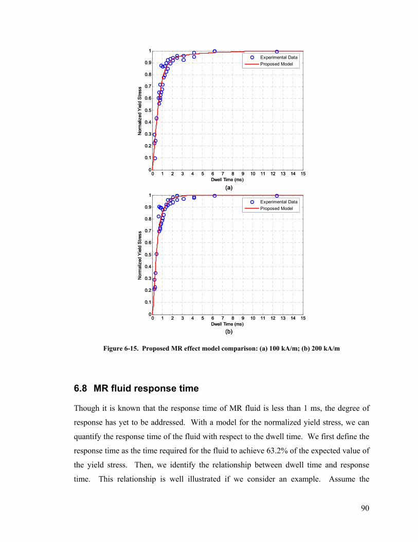
90
(a)
(b)
0 1 2 3 4 5 6 7 8 9 10 11 12 13 14 150
0.1
0.2
0.3
0.4
0.5
0.6
0.7
0.8
0.9
1
Dwell Time (ms)
Nor
mal
ized
Yie
ld S
tress
Experimental DataProposed Model
0 1 2 3 4 5 6 7 8 9 10 11 12 13 14 150
0.1
0.2
0.3
0.4
0.5
0.6
0.7
0.8
0.9
1
Dwell Time (ms)
Nor
mal
ized
Yie
ld S
tress
Experimental DataProposed Model
Figure 6-15. Proposed MR effect model comparison: (a) 100 kA/m; (b) 200 kA/m
6.8 MR fluid response time
Though it is known that the response time of MR fluid is less than 1 ms, the degree of
response has yet to be addressed. With a model for the normalized yield stress, we can
quantify the response time of the fluid with respect to the dwell time. We first define the
response time as the time required for the fluid to achieve 63.2% of the expected value of
the yield stress. Then, we identify the relationship between dwell time and response
time. This relationship is well illustrated if we consider an example. Assume the

91
response time of the fluid is 0.5 ms. Then, if the dwell time is greater than the response
time, the fluid will achieve greater than 63.2% of the expected yield stress. Otherwise,
the fluid will achieve less than 63.2% of the expected yield stress. From the models for
the normalized yield stress, we can identify the dwell time that corresponds to a
normalized yield stress of 0.632. This dwell time is the response time of the fluid.
The response time of the fluid for each magnetic field strength is identified in
Figure 6-16. With this scale, it is clear that magnetic field strength has a significant
effect on the normalized yield stress. The response times are identified graphically in
Figure 6-16 and summarized for each magnetic field strength in Table 6-2. As illustrated
in Figure 6-16, the response time decreases as magnetic field increases. This behavior
may be attributed to particle interaction within the fluid. A study by Ginder [75] suggests
that the pair-formation time is a function of field strength. Pair-formation is the
alignment of adjacent particles along magnetic flux paths. As the field is increased, the
pair-formation time decreases. The relationship suggested by Ginder is supported by the
results shown in Figure 6-16.
Table 6-2. Summary of response time results
Magnetic Field Strength (kA/m) Response Time (ms)
100 0.7325
200 0.5303
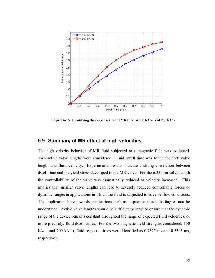
92
0 0.1 0.2 0.3 0.4 0.5 0.6 0.7 0.8 0.9 10
0.1
0.2
0.3
0.4
0.5
0.6
0.7
0.8
0.9
1
Dwell Time (ms)
Nor
mal
ized
Yie
ld S
tress
100 kA/m200 kA/m
Figure 6-16. Identifying the response time of MR fluid at 100 kA/m and 200 kA/m
6.9 Summary of MR effect at high velocities
The high velocity behavior of MR fluid subjected to a magnetic field was evaluated.
Two active valve lengths were considered. Fluid dwell time was found for each valve
length and fluid velocity. Experimental results indicate a strong correlation between
dwell time and the yield stress developed in the MR valve. For the 6.35 mm valve length
the controllability of the valve was dramatically reduced as velocity increased. This
implies that smaller valve lengths can lead to severely reduced controllable forces or
dynamic ranges in applications in which the fluid is subjected to adverse flow conditions.
The implication here towards applications such as impact or shock loading cannot be
understated. Active valve lengths should be sufficiently large to ensure that the dynamic
range of the device remains constant throughout the range of expected fluid velocities, or
more precisely, fluid dwell times. For the two magnetic field strengths considered, 100
kA/m and 200 kA/m, fluid response times were identified as 0.7325 ms and 0.5303 ms,
respectively.
93
Furthermore, from the normalized yield stress analysis, a model was proposed
which captures the dependence of yield stress on dwell time. Existing models for MR
fluid yield stress are functions of magnetic field strength exclusively. Based on the
results presented in this chapter, a modification of the form
( ) ( ){ }HCHtdwellpo ⋅⋅Φ⋅⋅⋅Ψ= 33.6tanh271700, 5239.1τ (6-20)
is suggested to account for the yield stress dependence on fluid dwell time.
94
7 Conclusions
This chapter summarizes the work conducted in this study. The primary results are
highlighted and suggestions are made for the extension of this work to future studies.
7.1 Research summary
This research studied the high shear and high velocity behavior of MR fluid. Since their
introduction, MR fluids and MR fluid devices have provided solutions to many
engineering challenges. The great success of MR fluids continues to motivate current
and future applications. However, while the behavior of the fluid may be well known
under certain operating conditions, current and future applications expose the fluid to, as
yet, uncharacterized flow conditions. Such conditions include high shear and high
velocity flow. This study identified the behavior of the fluid operating in these adverse
flow conditions. Both the off-state and the on-state behavior were evaluated.
The off-state behavior of the fluid was evaluated at shear rates ranging from
0.14x10⁵ s-1 to 2.5x10⁵ s-1. Because MR fluid behavior at high shear is largely governed
by the carrier fluid, the carrier fluid was also evaluated at high rates of shear. From the
measured force, the shear stress was found and the relationship between shear stress and
shear rate was presented for each fluid. Models for the high shear behavior of both the
MR fluid and the carrier fluid are developed from the experimental data. Results indicate
that MR fluid in the off-state exhibits nearly Newtonian post-yield behavior. A slight
thickening is observed for growing shear rates. This slight thickening may be largely due
to the carrier fluid behavior. At high shear, the carrier fluid exhibits considerable shear
thickening. This thickening may be the cause of the thickening observed in the MR fluid
behavior at high shear.
The goal of the on-state investigation was to characterize the MR effect at high
flow velocities. Fluid velocities ranged from 1 m/s to 37 m/s. Two active valve lengths
were considered, 25.4 mm and 6.35 mm. The term “dwell time” was introduced and
defined as the time the fluid spends in the presence of a magnetic field. For the range of
velocities considered and the two active valve lengths, corresponding fluid dwell times
95
ranged from 12 ms to 0.18 ms. Results indicate that fluid dwell time can greatly
influence the yield stress developed in the fluid. For dwell times less than 1 ms, the yield
stress may only achieve a fraction of the expected value. Furthermore, experimental
results imply that the normalized yield stress is a function of both dwell time and
magnetic field strength. A model which can describe the yield stress dependence on
dwell time and field strength is proposed. The model is well supported by the
experimental data.
In conclusion, this study evaluated the high shear and high velocity behavior of
MR fluid, both in the off-state and in the on-state. A nearly Newtonian post-yield
behavior was identified for the MR fluid in the off-state. Results for the on-state testing
indicated a need to consider fluid dwell times in high velocity applications. Active valve
lengths should be sufficiently large to ensure that the dynamic range of the device
remains constant throughout the range of expected fluid velocities, or more precisely,
fluid dwell times.
7.2 Recommendations for future research
Throughout the course of this research, several topics, beyond the scope of the current
study, were encountered. In what follows, a brief discussion of such topics is provided.
7.2.1 Non-steady conditions
The current study was conducted under steady-state conditions. In practice, however,
fluid flow within a particular device is seldom steady-state. On the contrary, the flow is
predominantly transient with many changes in flow direction and flow velocity. As a
first step, the current study serves to identify behavior under adverse steady-state
conditions. A logical extension would be to include adverse, non-steady conditions. Of
course, in developing models for the non-steady flow, the degree of difficulty associated
with the solution of the Navier-Stokes equations increases quite considerably. However,
various approximations or estimations can be made to simplify the problem. A number
of such approximations have been proposed in the literature [51, 56].
Of particular interest when considering non-steady conditions is the formation of
the plug within the flow channel. Under non-steady conditions the plug width would
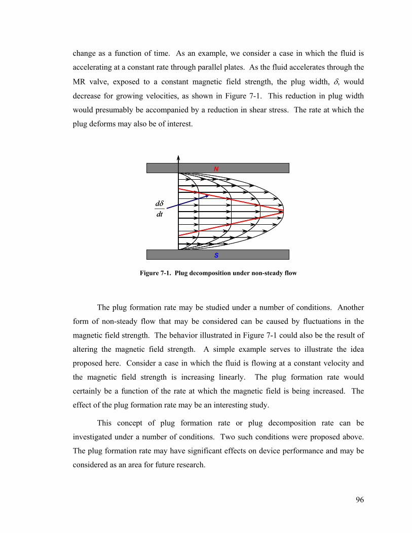
96
change as a function of time. As an example, we consider a case in which the fluid is
accelerating at a constant rate through parallel plates. As the fluid accelerates through the
MR valve, exposed to a constant magnetic field strength, the plug width, δ, would
decrease for growing velocities, as shown in Figure 7-1. This reduction in plug width
would presumably be accompanied by a reduction in shear stress. The rate at which the
plug deforms may also be of interest.
N
S
dtdδ
N
S
dtdδ
Figure 7-1. Plug decomposition under non-steady flow
The plug formation rate may be studied under a number of conditions. Another
form of non-steady flow that may be considered can be caused by fluctuations in the
magnetic field strength. The behavior illustrated in Figure 7-1 could also be the result of
altering the magnetic field strength. A simple example serves to illustrate the idea
proposed here. Consider a case in which the fluid is flowing at a constant velocity and
the magnetic field strength is increasing linearly. The plug formation rate would
certainly be a function of the rate at which the magnetic field is being increased. The
effect of the plug formation rate may be an interesting study.
This concept of plug formation rate or plug decomposition rate can be
investigated under a number of conditions. Two such conditions were proposed above.
The plug formation rate may have significant effects on device performance and may be
considered as an area for future research.

97
7.2.2 Evaluating different MR fluid compositions
The MR fluid used in this study was MRF-132LD. This particular fluid had an iron
content of 32% by volume. Future studies might consider the effect of iron content to
identify the effect of iron content on the behavior of the fluid at high velocities and high
shear rates; higher iron content may lead to faster response times. A number of fluids are
commercially available from Lord Corporation with varying fluid compositions. For
high velocity applications, future work might identify which existing fluid is best suited
for such applications. Furthermore, a thorough study might identify which fluid
properties are responsible for the improved performance at high velocity and high shear.
This information may prove valuable in the development of future fluids specifically
engineered for high velocity and high shear applications.
7.2.3 Other recommendations
Throughout the course of the current study, several other thoughts and ideas were come
upon. These may be developed into avenues for future research and are summarized as
follows:
• Identify the dependence on normalized yield stress on magnetic field strength –
Future work may include a number of additional experiments performed at
various magnetic field strengths. With sufficient data to represent the magnetic
field dependence, it will be possible to further develop the proposed model for the
normalized yield stress such that it can be expressed explicitly as a function of
both dwell time and magnetic field strength.
• Identify a model for the response time of MR fluid as a function of magnetic field
strength
• Investigate the dependence of particle size and shape on the high velocity and
high shear behavior of MR fluid
• Study the effect of the off-state behavior on the high velocity on-state behavior –
How does the off-state viscosity effect the on-state behavior of the fluid at high
velocity and high shear?

98
References
1. Rabinow, J., “The magnetic fluid clutch,” AIEE Trans. 67, p. 1308, 1948.
2. Weiss, K. D., Duclos, T. G., Carlson, J. D., Chrzan, M. J., Margida, A. J., “High strength magneto – and electro – rheological fluids,” Society of Automotive Engineers, 932451, 1993.
3. Carlson, J. D., Weiss, K. D., “A growing attraction to magnetic fluids,” Machine Design, Vol. 66, No. 15, p. 61-64, 1994.
4. Lord Corporation, www.lord.com
5. Carlson, J. D., “Multi-degree of freedom magnetorheological devices and system for using same,” U.S. Patent 5,492,312 1996.
6. Hong, S. R., Choi, S. B., Jung, W. J., Jeong, W. B., “Vibration isolation of Structural Systems Using Squeeze Mode ER Mounts,” Journal of Intelligent Material Systems and Structures, Vol. 13, No. 7, p. 421-424, 2002.
7. Carlson, J. D., and Jolly, M. R., “MR fluid, foam and elastomer devices,” Mechatronics, 10, p. 555-569, 2000.
8. Jolly, M. R., Bender, J. W., and Carlson, J. D., “Properties and applications of commercial magnetorheological fluids,” Journal of Intelligent Material Systems and Structures, Vol. 10, No. 1, p. 5, 1999.
9. Koo, J. H., “Using magnetorheological dampers in semiactive tuned vibration absorbers to control structural vibrations,” Ph.D. Dissertation, Virginia Polytechnic Institute and State University, Blacksburg, VA, 2003.
10. Crosby, M. J., Karnopp, D. C., “The Active Damper,” The Shock and Vibration Bulletin 43, Naval Research Laboratory, Washington, DC, 1973.
11. Karnopp, D. C., Crosby, M. J., “System for controlling the transmission of energy between spaced members,” U.S. Patent 3,807,678 1974.
12. Lee, H. S., and Choi, S. B., “Control and response characteristics of a magnetorheological fluid damper for passenger vehicles,” Journal of Intelligent Material Systems and Structures, Vol. 11, No. 1, p. 80-87, 2000.
13. Simon, D. E., “An investigation of the effectiveness of skyhook supsensions for controlling roll dynamics of sport utility vehicles using magnetorheological dampers,” Ph.D. Dissertation, Virginia Polytechnic Institute and State University, Blacksburg, VA, 2001.
14. Song, X., Ahmadian, M., Southward, S. C., "An Adaptive Semiactive Control Algorithm for Vehicle Suspension Systems," Proceedings of IMECE, Washington, D.C., November 16 - 21, 2003.
15. Pund, D., Markus, F., Robinson, A., Webster, L., “The New Cars: Charting the Changes for 2002,” Car & Driver, Vol. 47, No. 4, p. 62, Oct. 2001.
99
16. Gehm, R., “Delphi Improves Cadillac’s Ride,” Automotive Engineering International, Vol. 109, No. 10, pp. 32-33, Oct. 2001.
17. Halverson, H., “Magnetic Ride - Star Wars Meets the 50th Car,” www.corvetteactioncenter.com, 2003.
18. Lord Rheonetic Magnetically Responsive Technology, MR Damper, RD-1005-3 Product Bulletin, 2003.
19. Carlson, J. D., Catanzarite, D. M., St. Clair, K. A., "Commercial Magneto-Rheological Fluid Devices,” Proceedings 5th International Conference on ER Fluids, MR Suspensions and Associated Technology, W. Bullough, Ed., World Scientific, Singapore, 1996.
20. Wu, X., and Griffin, M. J., “A Semi-Active Control Policy to Reduce the Occurrence and Severity of End-Stop Impacts in a Suspension Seat with and Electrorheological Fluid Damper,” Journal of Sound and Vibration, Vol. 203, No. 5, p. 781-793, 1997.
21. Choi, S. B., Nam, M. H., Lee, B. K., “Vibration Control of MR Seat Damper for Commercial Vehicles,” Journal of Intelligent Materials System and Structures, Vol. 11, No. 12, p. 936-944, 2000.
22. McManus, S. J., St. Clair, K. A., Boileau, P. E., Boutin, J., “Evaluation of Vibration and Shock Attenuation Performance of a suspension Seat with a Semi-Active Magnetorheological Fluid Damper,” Journal of Sound and Vibration, Vol. 253, No. 1, p. 313-327, 2002.
23. Choi, Y. T., and Wereley, N. M., “Mitigation of Biodynamic Response to Vibratory and Blast-Induced Shock Loads Using Magnetorheological Seat Suspensions,” Proceedings of IMECE, 43313, Washington, D.C., November, 16-21, 2003.
24. Lord Corporation, “Sears Seating Taps LORD Corporation to Provide Motion Master Seat Suspension Technology for Ag, Off-Highway Vehicles,” Press Release, September, 2003.
25. Lord Corporation, “School Transportation Officials in Six States Adopt LORD Corporation’s Driver Seat System for Bus Safety,” Press Release, August, 2001.
26. Dyke, S. J., Spencer Jr., B. F., Sain, M. K., Carlson, J. D., “Modeling and Control of Magnetorheological Dampers for Seismic Response Reduction,” Smart Materials and Structures, Vol. 5, No. 5, p. 565-575, 1996.
27. Dyke, S. J., Spencer Jr., B. F., Sain, M. K., Carlson, J. D., “An Experimental Study of MR Dampers for Seismic Protection,” Smart Materials and Structures, Vol. 7, No. 5, p. 693-703, 1998.
28. Carlson, J. D., Spencer Jr., B. F., “Magnetorheological Fluid Dampers for Seismic Control,” Proceedings of DETC, VIB4124, Sacramento, CA, 1997.
29. Yang, G., Spencer Jr., B. F., Carlson, J. D., Sain, M. K., “Large-scale MR Fluid Dampers: Modeling and Dynamic Performance Considerations,” Engineering Structures, 24, p. 309-323, 2002.
100
30. Ni, J. M., Ni, Y. Q., Chen, Z. Q., and Spencer Jr., B. F., “Implementation of MR Dampers to Dongting Lake Bridge for Cable Vibration Mitigation,” Proceedings of the 3rd World Conference on Structural Control, Como, Italy, Vol. 3, p. 777-786, 2002.
31. Ni, Y. Q., Chen, Z. Q., Ko, J. M., and Zheng, G., “Optimal Voltage/Current Input to ER/MR Dampers for Multi-switch Control of Stay Cable Vibration,” Proceedings of the 3rd World Conference on Structural Control, Como, Italy, Vol. 3, p. 767-775, 2002.
32. Lord Corporation, “LORD Corporation Supplies 320 MR Fluid Dampers for Cable-Stayed Bridge Retrofit to Control Wind Vibration,” Press Release, March, 2002.
33. Carlson, J. D., “Low-Cost MR Fluid Sponge Devices,” Journal of Intelligent Material Systems and Structures, Vol. 10, p.589-594, August, 1999.
34. Biedermann Motech GmbH, www.biedermann.com
35. Carlson, J. D., Matthis, W., Toscano, J. R., “Smart Prosthetics Based on Magnetorheological Fluids,” Proceedings of SPIE, Vol. 4332, p. 308-316, 2001.
36. Lord Rheonetic Magnetically Responsive Technology, MR Brake MRB-2107-3, Product Bulletin, 2003.
37. QED Technologies, www.qedmrf.com
38. Kordonski, W. I., and Golini, D., “Fundamentals of Magnetorheological Fluid Utilization in High Precision Finishing,” Journal of Intelligent Material Systems and Structures, Vol. 10, p. 683-689, September, 1999.
39. Menapace, J. A., Dixit, S. N., Genin, F. Y., Brocious, W. F., “Magnetorheological Finishing for Imprinting Continuous Phase Plate Structure onto Optical Surfaces,” UCRL-CONF-153850, Boulder Damage Sysmposium XXXV, Boulder, CO, September 21-24, 2003.
40. Ahmadian, M., Poynor, J. C., Gooch, J. M., “Application of Magneto Rheological Dampers for Controlling Shock Loading,” Proceedings of ASME Dynamic Systems and Control, DSC-Vol. 67, p. 731-735, 1999.
41. Messina, N., “Multi-Role Armament & Ammunition System ATD-GDAS Program Scope and Approach,” Proceedings of 36th Annual Gun & Ammunition Symposium & Exhibition, www.dtic.mil/ndia, presentation, April 9-12, 2004.
42. Chen, P. C., Wereley, N., “Magnetorheological Damper and Energy Dissipation Method,” U.S. Patent 6,694,856 B1 2004.
43. Facey, W. B., Rosenfeld, N. C., Choi, Y. T., Wereley, N. M., “Design and Testing of a Compact Magnetorheological Damper for High Impulsive Loads,” Proceedings of the 9th International Conference on Electrorheological Fluids and Magnetorheological Suspensions, Beijing, China, August 29 – September 3, 2004.
101
44. El Wahed, A. K., Sproston, J. L., Schleyer, G. K., “Electrorheological and Magnetorheological Fluids in Blast Resistant Design Applications,” Materials and Design, 23, p. 391-404, 2002.
45. El Wahed, A. K., Sproston, J. L., Schleyer, G. K., “A Comparison Between Electrorheological and Magnetorheological Fluids Subjected to Impulsive Loads,” Proceedings of the 7th International Conference on Electrorheological Fluids and Magnetorheological Suspensions, Honolulu, Hawaii, p. 401-410, 1998.
46. Norris, J. A., “Behavior of Magnetorheological Fluids Subject to Impact and Shock Loading,” M.S. Thesis, Virginia Polytechnic Institute and State University, Blacksburg, VA, 2003.
47. Browne, A. L., McCleary, J. D., Namuduri, C. S., Webb, S. R., “Impact Performance of Magnetorheological Fluids,” Proceedings of IMECE, 60542, Anaheim, CA, November, 13-20, 2004.
48. Choi, Y. T., Wereley, N. M., “Vibration Control of a Landing Gear System Featuring Electrorheological/Magnetorheological Fluids,” Journal of Aircraft, Vol. 40, No. 3, p. 432-439, 2003.
49. Carlson, J. D., “What Makes a Good MR Fluid?,” Journal of Intelligent Material Systems and Structures, Vol. 13, No. 7, p. 431-435, 2002.
50. Lord Corporation, “Army Looks at Improving Vehicles’ Performance with MR Fluid Technology from LORD Corporation,” Press Release, July, 2004.
51. Phillips, R. W., “Engineering Applications of Fluids with a Variable Yield Stress,” Ph.D. Dissertation, University of California, Berkeley, CA, 1969.
52. Yang, G., “Large-Scale Magnetorheological Fluid Damper for Vibration Mitigation: Modeling, Testing and Control,” Ph.D. Dissertation, University of Notre Dame, Notre Dame, IN, 2001.
53. Kamath, G. M., Hurt, M. K., Wereley, N. M., “Analysis and Testing of Bingham Plastic Behavior in Semi-Active Electrorheological Fluid Dampers,” Smart Materials and Structures, Vol. 5, p. 576-590, 1996.
54. Wereley, N. M., Pang, L., “Nondimensional Analysis of Semi-Active Electrorheological and Magnetorheological Dampers Using Approximate Parallel Plate Models,” Smart Materials and Structures, Vol. 7, p. 732-743, 1998.
55. Constantinescu, V. N., Laminar Viscous Flow, Springer, New York, 1995.
56. Gavin, H. P., “Electrorheological Dampers for Structural Vibration Suppression,” Ph.D. Dissertation, University of Michigan, Ann Arbor, MI, 1994.
57. Beyer, W. H., CRC Handbook of Mathematical Sciences, 6th Edition, CRC Press, Boca Raton, FL, 1987.
58. Jolly, M. R., Carlson, J. D., Munoz, B. C., “A Model of the Behavior of Magnetorheological Materials,” Smart Materials and Structures, Vol. 5, p. 607-614, 1996.
102
59. Lord Rheonetic Magnetically Responsive Technology, Hydrocarbon-Based MR Fluid MRF-132LD, Product Bulletin, 2002.
60. Carlson, J. D., “MR Technology Workshop – Chapter 6,” Lord Corporation, Cary, NC, p. 6/9-6/10, 2004.
61. 1989 ASHRAE Handbook – Fundamentals.
62. Baird, D. G., and Collias, D. I., Polymer Processing Principles and Design, Wiley Interscience, New York, NY, 1998.
63. Van Wazer, J. R., Lyons, J. W., Kim, K. Y., Colwell, R. E., Viscosity and Flow Measurement A Laboratory Handbook of Rheology, Wiley Interscience, New York, NY, 1963.
64. Lord Materials Division, “Magnetic Circuit Design,” Engineering Note, 1999.
65. Carlson, J. D., “Magnetorheological Fluid Seismic Damper,” U.S. Patent, 6,296,088 B1 2001.
66. BASF, The Chemical Company, www.BASF.de.
67. Material Safety Data Sheet (MSDS #3332), Synfluid ® 4 cSt PAO, Chevron Phillips Chemical Company LP, The Woodlands, TX, Rev. 19, Rev. Date 10/07/2004.
68. Carlson, J. D., Private communication, 2004.
69. Incropera, F. P., DeWitt, D. P., Introduction to Heat Transfer, John Wiley & Sons, New York, 1990.
70. Lord Materials Division, “MR Valve Configurations,” Engineering Note, 2001.
71. Carlson, J. D., Chrzan, M. J., “Magnetorheological Fluid Dampers,” U.S. Patent, 5,277,281 1994.
72. Carlson, J. D., Chrzan, M. J., James, F. O., “Magnetorheological Fluid Devices,” U.S. Patent, 5,398,917 1995.
73. Poynor, J. C., “Innovative Designs for Magnetorheological Dampers,” M.S. Thesis, Virginia Polytechnic Institute and State University, Blacksburg, VA, 2001.
74. Bullough, W. A., Peel, D. J., Spronston, J. L., Stanway, R., Rodgers, D. L., “An ER Long-Stroke Damper for Vehicle Suspension Applications,” FED-Vol. 205/AMD-Vol. 190, p. 41, Proceedings of IMECE, Chicago, Illinois, November 6-11, 1994.
75. Ginder, J. M., “Rheology Controlled by Magnetic Fields,” Encyclopedia of Applied Physics, Vol. 16, p. 487-503, 1996.

103
Vita
Fernando D. Goncalves was born on August 28th, 1977 in Floral Park, New York. He
grew up in nearby Farmingville, New York, where his parents still live today. Fernando
graduated in 1995 from Sachem High School in Lake Ronkonkoma, New York. From
there, he went on to pursue a degree in Engineering from Roger Williams University in
Bristol, Rhode Island. In 1999, he earned his Bachelor’s degree in Engineering,
graduating Cum Laude and first in the School of Engineering. After graduating,
Fernando headed south to pursue a M.S. degree in Mechanical Engineering from Virginia
Tech in Blacksburg, Virginia. Studying in the Advanced Vehicle Dynamics Laboratory,
Fernando’s M.S. work focused on semi-active vehicle suspensions. Earning his M.S.
degree in August of 2001, Fernando remained at Virginia Tech to begin Ph.D. studies.
His Ph.D. work focused on the high velocity flow of magnetorheological fluids.
Fernando earned his Ph.D. in May 2005 and has accepted a position at Lord Corporation
in Cary, North Carolina. Fernando will be married in September 2005 to his fiancée
Courtney Mulligan.