Analysis of Protein

Structure and Function: A Beginner's Guide to CHARMM

Robert Schleif

Biology Department

Johns Hopkins University

3400 N. Charles St. Baltimore, MD 21218

1/2/06

ii

Preface Increasingly, biologists and biochemists are faced with understanding how their favorite proteins work. The structures of many of these proteins have been determined, and the structures of many more will be determined in the next few years. Once a protein's structure has been determined, it becomes possible and also enticing to design experiments probing the protein's mechanism of action. Tools for the graphical display of structure, the manipulation of the structure, and the calculation of various interaction energies all become interesting and important. Additionally, some properties of a protein may best be revealed by modeling the protein in water and simulating its molecular thermal motion at 300 K.

A researcher interested in protein structure and function faces the question of whether to use one of the complete, but expensive, computer programs for the manipulation and analysis of protein structure, use a number of the highly specialized but almost completely undocumented programs that are available on the web, or to learn and use a powerful and general program that can perform most of the manipulations and calculations one might need. This book is written for those who decide to follow the latter course and to learn the program CHARMM (Chemistry at Harvard Macromolecular Mechanics) that was initiated in the laboratory of Dr. Martin Karplus. The program has been continuously refined and extended by many workers over the years since the initial publication, "CHARMM: A Program for Macromolecular Energy, Minimization, and Dynamics Calculations", J. Comp. Chem. 4, 187-217 (1983), by B. R. Brooks, R. E. Bruccoleri, B. D. Olafson, D. J. States, S. Swaminathan, and M. Karplus. This book describes the use of the program for structure analysis, model building, energy calculations, and dynamics simulations. Additionally, the program can perform Monte Carlo calculations, normal mode analysis, free energy calculations, and incorporate quantum mechanical calculations.

iii

Contents

CHAPTER 1 FUNDAMENTALS

Introduction .............................................................................................................................. 1

Required Hardware, Software, and Computer Expertise ......................................................... 1

The Flavor of Linux.................................................................................................................. 2

Sources of Information ............................................................................................................. 4

Installing, Testing, and Basic Operation of CHARMM........................................................... 5

Cartesian and Internal Coordinate Systems.............................................................................. 8

Forces and Potential Energy ..................................................................................................... 9

Hydrogen Bonds and CHARMM ........................................................................................... 13

Methods of Dynamics Calculations........................................................................................ 13

The Verlet Propagation Algorithm......................................................................................... 14

Achieving Precise but Convenient Structural Description of Systems .................................. 15

Description of Polymer Units, the Residue Topology File, RTF ........................................... 15

Definition of Atom Properties and Interactions, the Parameters File, PARA........................ 17

Coordinate Files...................................................................................................................... 18

Description of a Complete System, The Principle Structure File, PSF.................................. 19

Explicit and Implicit Representation of Water ....................................................................... 20

Arrays, and Built-in Substitution Parameters ......................................................................... 22

Atom Selection ....................................................................................................................... 23

Units ....................................................................................................................................... 27

More Useful Linux Commands .............................................................................................. 27

Some Refinements to CHARMM Scripts .............................................................................. 29

Problems................................................................................................................................. 31

iv

Bibliography ........................................................................................................................... 32

Related Web Sites .................................................................................................................. 33

CHAPTER 2 INPUTTING FILES AND COORDINATE CALCULATIONS

Reformatting Protein Data Bank Files for Input to CHARMM ............................................. 34

Using awk to Reformat Protein Data Bank Files ................................................................... 37

Providing Missing Atoms and Coordinates............................................................................ 40

Reading AraC into CHARMM............................................................................................... 42

Phi-Psi Angles in Proteins ...................................................................................................... 48

Determining Phi-Psi Angles in AraC ..................................................................................... 49

Coordinate Manipulation Commands--Using CHARMM Documentation ........................... 53

Surface Area, Cavities and Holes in Proteins......................................................................... 54

Solvent Exposure of Residues in AraC .................................................................................. 56

Looping, Loop Counters, and Calculation of Unfolded Surface Area ................................... 58

Finding Cavities and Holes in AraC....................................................................................... 60

Handling Multisubunit Proteins and Reading in Multiple Coordinate Files.......................... 63

Identifying Residues Constituting a Dimerization Interface .................................................. 64

RMS Overlaying Structurally Similar Molecules................................................................... 66

Asymmetric Units, Biological Molecules and Unit Cells ...................................................... 71

Translating and Rotating a Subunit or Protein With Awk and With CHARMM .................. 73

Constructing the Biological Dimer of Apo-AraC Protein and a Linux-CHARMM TRICK . 75

Area of the Dimerization Interface of AraC ........................................................................... 79

Distance Maps-Secondary Structure Identification in AraC .................................................. 82

Distance Difference Maps, Application to Hemoglobin ........................................................ 85

Problems................................................................................................................................. 90

Bibliography ........................................................................................................................... 90

v

Related Web Sites .................................................................................................................. 91

CHAPTER 3 ENERGY MINIMIZATION AND RUNNING DYNAMICS SIMULATIONS

Methods of Energy Minimization........................................................................................... 93

Energy Minimizing the Dimerization Domain of AraC......................................................... 94

Considerations for a Dynamics Simulation ............................................................................ 97

A Dynamics Run with the AraC Dimerization Domain....................................................... 101

Langevin Dynamics .............................................................................................................. 112

A Langevin Simulation of the AraC Dimerization Domain................................................. 113

A Simulation with Periodic Boundary Conditions............................................................... 114

Reading Trajectories............................................................................................................. 116

Calculating and Interaction Energy at Intervals During a Trajectory................................... 117

Writing out PDB Format Coordinates from a Trajectory File.............................................. 119

Time Series Analysis, Reading Rotamer Angles.................................................................. 119

Problems............................................................................................................................... 123

Bibliography ......................................................................................................................... 123

Related Web Sites ................................................................................................................ 124

CHAPTER 4 MODEL BUILDING

Building a Box of Water....................................................................................................... 125

Constructing an Alpha Helix, Beta Sheet, Polyproline II Helix and Regular Structures ..... 129

Fixing, Restraining, and Pulling Atoms ............................................................................... 131

Changing, or Mutating Residues .......................................................................................... 133

Adjusting Rotameric State.................................................................................................... 135

Use of Patches for Special Structures................................................................................... 137

Constructing a Quick and Dirty Patch for the GFP Chromophore....................................... 138

vi

Writing a Residue Topology File Ligand Entry for Arabinose ............................................ 140

Fusing Two Peptides ............................................................................................................ 144

Patches for Working with DNA ........................................................................................... 146

An Alternative for Inputting DNA ....................................................................................... 150

Adding Counterions to DNA............................................................................................... 152

Problems............................................................................................................................... 156

Bibliography ......................................................................................................................... 156

Related Web Sites ................................................................................................................ 157

APPENDICES

System or CHARMM Modifications ................................................................................... 158

Command Line Substitution Parameters .............................................................................. 158

TABLES

1

Chapter 1

Fundamentals

Introduction

The calculations and manipulations that one can do with the CHARMM molecular mechanics program facilitate the study of protein structure and function. This book is intended to show and teach some of the aspects of protein structure and function that can be analyzed computationally and how to do them with CHARMM. This will be done through the use of many examples and many complete programs, which are usually called scripts, for running CHARMM. The example scripts and critical portions of the output they generate illustrate how to use the program in structure analysis, model building, energy analysis, and analysis of the motions of proteins.

Many of the calculations that are possible with CHARMM, like determination of exposed surface area or the strength of interaction between two sets of amino acids, can be interpreted in a straightforward manner. Most of the calculations presented in this book are of this nature. The results of some calculations however, like the analysis of a dynamics simulation run, can be more ambiguous. One's own scientific experience and skill play an important part in the design and interpretation of these calculations because what molecular dynamics simulation of proteins can and cannot tell us about protein function is still being learned. Up to this point CHARMM seems to have been used largely by those working on the development of molecular dynamics. That does not prevent others, the intended readers of this book, who are interested in the application of the many tools that CHARMM provides, from using them.

Required Hardware, Software, and Computer Expertise

Although computer networks or supercomputers are often utilized for lengthy and large molecular dynamics simulations, a simple single or dual processor desktop computer with at least 40GB hard drive space, a CD-ROM writer, more than 300 MB RAM, and an internet connection is more than adequate for much work. To give some idea of the speeds of computation, throughout this book, the times required to run many of the scripts and operations on a machine running at about 1 Ghz will be mentioned if they exceed 60 seconds. These timings are approximate. Not only does the clock speed, but also the computer design and even the processor design can affect overall computation speed. For example, earlier Intel processors outperformed some later processors operating at much higher clock speeds because the former processors performed more complex operations per clock cycle than the later processors.

The CHARMM program runs under the Unix-Linux operating systems. Since most of the potential users of this book are likely to be using personal computers running the Linux operating system, the term Linux will be used, even though for purposes of running CHARMM there are no real differences between Linux and Unix. Installation of Linux on a personal computer usually is simple and can be performed by novices using packages obtained from sources such as Red Hat. Problems in installation can be completely avoided by purchasing a computer with Linux installed. To carry out the operations described in this book, the reader will need to become familiar with the simple navigation and maintenance commands of Linux like change directory, list files, remove and copy files, and the editing of files. These operations can all be carried out in

2

Linux with graphical interfaces that are provided with the popular packages like Linux Red Hat. As CHARMM is run from the command line it will also be necessary to become familiar with this mode of controlling a computer. Many popular books describe the installation and use of Linux. Two books from O’Reilly Publishing, “Unix for Beginners” and “Linux in a Nutshell” are most helpful for learning and using Linux. It is also helpful to have access to sufficient Linux expertise that an internet connection can be made and programs can be installed. Although the installation and use of CHARMM and Linux are quite simple, using Linux is not the same as using the Mac or Windows operating systems, and seemingly obscure problems can occasionally arise.

It is not necessary to be a skilled programmer to start to use the approaches described in this book. One must, however, be able to understand the basic concepts that are used in programming so that the scripts and program examples provided here can be modified as needed. Complete and working scripts and programs are presented for many of the operations discussed, and most related problems can be addressed by using components from these scripts and programs.

A good molecular graphics program is essential for display of the macromolecules being manipulated by CHARMM. The program known as VMD (Humphrey et. al. 1996), which can be obtained free over the internet http://www.ks.uiuc.edu/Research/vmd/ can be recommended. This program can use a variety of input file types, including trajectory files from molecular dynamics simulation runs. Quite often, the final processing and plotting of data from CHARMM can most conveniently be done with a spreadsheet program.

The Flavor of Linux

The Windows and Mac operating systems provide interfaces that allow almost intuitive operation of the computer and the programs installed on it. These two operating systems are also designed to be used by only a single user. The Unix and Linux operating systems are designed to accommodate multiple users as well as multiple simultaneous users, and the assumption is also made that the users may not be competent, friendly, or honest. Thus, these systems are constructed to isolate each user from potentially harmful effects or even malicious efforts of other users. Hence, one must log onto the computer and provide a password to be allowed access to one's own files. One can also prevent others from reading, reading or writing, or reading, writing, and executing one's files. Similarly, only a trusted user called the root user is allowed to make important changes in the operating system or the way it functions. These protections somewhat complicate the use of Linux but do generate a relatively secure multi-user environment. Below a very brief outline of the use of Linux is provided. Other sources, for example, "Learning the Unix Operating System" by Grace Todino, John Stran, and Jerry Peek, and “Linux in a Nutshell” 4th ed. by Siever, E., Figgins, S. and Weber, A. should be consulted for much more thorough discussions and explanations.

Directories in Linux are the same as folders on the Mac operating system or directories in Windows. The top (perhaps bottom is more appropriate) of the Linux directory structure is known as the root, and it is designated with the slash symbol, /. Directories and subdirectories branch off from it, and the location of a user's personal files might be in a subdirectory called bob which is a subdirectory in home which is a subdirectory in root. The location of the bob

3

subdirectory would then be /home/bob. Here we see the slash symbol designating root as well as serving as a separator between the name of a directory and a subdirectory.

While a good many of the standard operations one may need to perform on a computer running Linux can be performed graphically as they are done with the Windows or Mac operating systems, many more are easily performed through the command line interface. This is accessed in an open and active terminal window. Near the top left of the window will be some text and the active cursor. The text that is displayed can be adjusted as described in instructions for using the Linux operating system. For example, the system could be set to show the name of the user, the name of the computer, and the current directory. This information would be displayed as [bob@kinetic bob]$

The prompt symbol in this operating setup is the dollar sign, $. A command can be entered at the prompt by typing on the keyboard, and it will be executed when the enter key is pressed. For example, the command ls instructs the operating system to list the files in the current directory. This list will appear below the command, and if the list is long, may even scroll the command off the top of the window.

Much documentation on the use of Linux is contained on the computer and the user should become familiar with extracting it. For example, information, in fact more information than one would ever seem to need, on many Linux commands can be obtained simply by typing man, for manual, at the command prompt followed by the command name. For example, man ls gives information on the ls command. Up to a screen full of the information is displayed at once. The next screen full can be displayed by pressing the spacebar, and it is possible to move backwards through a series of screens by pressing b. To quit viewing the information from man, press q. Many of the Linux commands that are used at the command line possess variants and options. For example, the manual on the ls command explains that the l option, for long, instructs ls to list not only the file names in a directory, but also several other pieces of information. The l option would be specified as ls -l.

Some other useful commands are cp fileA fileB, which will generate a copy of fileA, naming it fileB, rm fileA, which will remove or delete fileA, and mkdir nameA, which creates a directory named nameA. Issues of permissions may complicate file removal. You can remove a file only if you have permission to write to the file and to the directory in which the file resides. Permissions can be determined and adjusted to allow reading, writing, or executing with one of the graphical programs, or at the command line. Permissions of files can be determined with the long option of ls, ls –l, and they may be changed with the command chmod. For example, to add read, r, and write, w, and remove execute, x, permission from a file named dna, the command would be chmod +r+w-x dna.

Suppose the bob directory contained a subdirectory named charmm and another named coordinates. To change one's location from the bob subdirectory to the charmm subdirectory, the command cd charmm would be entered at the prompt. The prompt line could now read [bob@kinetic charmm]$

4

Another way to verify what directory you are in would be to enter the command pwd, which stands for print working directory. The following line would then appear. /home/bob/charmm [bob@kinetic charmm]$

One could change back to the bob directory with the command cd /home/bob. In this case, the complete path from the root to the desired directory has been written. Another way would be cd .. where the double dot signifies the directory one level earlier in the directory tree. One could change from the coordinate directory to the charmm directory in two steps, for example, cd .. followed by cd charmm, or one could make the change in one step with cd ../charmm, or with cd /home/charmm.

Two especially powerful Linux-Unix “commands” deserve special attention. They are grep and awk. Because effective use of CHARMM requires some facility in the use of these two programs, whenever possible, the auxiliary use of these programs will be included and described along with the use of CHARMM itself. Grep is a powerful searching program that returns lines from files that satisfy a searching criterion. Often this capability is useful in extracting data from the voluminous output of CHARMM because as a script runs, CHARMM describes each step of the operation and often generates thousands of lines of output for even a small calculation or short simulation. Grep is also useful in searching for text stored on the computer, for example, to locate documentation on the computer or on CHARMM. Awk is a line-based editing program that searches for lines meeting criteria you have specified. It will then carry out various operations on the information that is contained on those lines. Because much of the input data to CHARMM is contained in lines listing atomic coordinates and because much of the output consists of lines of a reproducible structure that contain the desired data, awk is valuable both in the preparation of data for use by CHARMM and in the analysis of output from CHARMM.

Sources of Information

Information necessary for running CHARMM is contained in documentation files that accompany the program and can also be found at a number of sites on the web. These documentation files can be displayed on the computer, and can also be printed out. In the text, a reference to the relevant CHARMM document will be made by placing the document name in parenthesis, for example, (usage.doc). This documentation is not, however, an easy way to learn how to use CHARMM. The documentation was written by experts, and is for experts. Additionally, each section is written assuming that you understand all the other sections. Despite their unsuitability as a learning tool, the eighty or so files on different CHARMM topics must frequently be referred to in the course of using CHARMM.

The most convenient access to CHARMM’s documentation is via a web browser directed to this documentation in html format. The multiple links within this form of the documentation greatly facilitate navigation to the desired information. A number of such sites exist on the web and one can also install this documentation in one’s own computer that runs either the Windows or Linux operating system.

5

The absence of an index to the documentation can be overcome most easily by using Google to search. For example, “charmm energy documentation”. Searching can also be done by using the Linux command grep to identify files that contain a particular word. For example, grep -r "force" /usr/local/c29b1/doc | more

searches for the word force in /usr/local/c29b1/doc and its subdirectories. Locally installed programs often are contained in /usr/local, and the subdirectory c29b1 is the name of a directory containing CHARMM in this example. Grep outputs the names of files containing the search term and the line in the file that contained the term. The -r option instructs grep to search subdirectories as well, and the vertical bar is the command to the operating system for sending the output from grep directly into the more command. More allows viewing its input one screen at a time. It displays one screen and stops until the spacebar is depressed, at which time more displays the second screen, and so on. To escape from more, press the q key. We have already seen the more command in operation, as the output from the man command is automatically routed through more. If in the grep search described above, a narrower search term had been used, the output would have been smaller, and the | more portion of the command would have been unnecessary.

Linux is not completely uniform in its structure. In searching for a file of a specific name using the find command, it is not necessary to specify searching subdirectories. This is done automatically. The following will look for a file named "toph19_eef1.inp" on a system in which charmm29b1 has been installed in the /usr/src/c29b1 directory. As issued, find searches the directory c29b1 and all subdirectories for a file with the name as given, and then displays the result on the monitor. find /usr/local/src/c29b1 -name 'toph19_eef1.inp' -print

Another source of information that is provided with CHARMM is its suite of test cases. These are located in the test subdirectory of the CHARMM installation directory. Often the appropriate test script is hard to find and highly cryptic, but occasionally proves useful.

Many excellent web sites contain information about molecular modeling and molecular dynamics and describe running CHARMM. Most of these are compiled from notes for graduate level molecular modeling courses. Typically they outline the biophysical basis of molecular dynamics and then illustrate relatively problem-free simulations of simple systems. With persistent searching, the answers to most questions can be found on the web. One notable web source is the CHARMM forum. This is moderated by the major CHARMM experts.

A number of books describe molecular dynamics theory and are good sources of information about the topic, (Brooks et al. (1988), Rapaport, (1995), Allen et al. (1987), Frenkel and Smit (1996), Haile, (1992), Leach, (2001).

Installing, Testing, and Basic Operation of CHARMM

A license to run CHARMM currently can be purchased for a nominal fee as described on the CHARMM website, http://yuri.harvard.edu/. The program is provided on a CD that contains the documentation, source code, and necessary auxiliary files in an archived form known as a tar file.

6

It is probably best not to copy the tar file into one’s own directory or to install it there, but rather to put the files into a location that is convenient for multiple users. To install CHARMM anywhere other than in one’s own directory, one must be logged onto the computer as the root user. Then it is necessary to “mount” the CD on which CHARMM is provided. This is more than just putting the CD in the drive, it also means informing Linux that the CD is now to be considered part of the file system of the computer. Mounting can be done with the system disk management utility or from the command line. Then a graphical program for manipulating files can be used to copy the archived program, c29b1.tar to the directory where CHARMM is to be located. This will be /usr/src in the following example. The archived files are extracted by first changing to the /usr/src directory, and then entering tar –xvf c29b1.tar at the command prompt. The subdirectories doc, exec, lib, source, support, test, tool, and toppar are created and various files constituting the source code for CHARMM and various auxiliary files are extracted and placed in them. Additionally, a file called install.com is placed in the c29b1 directory.

As described in the instructions, (install.doc), the default version of an executable version of CHARMM on a Linux system can be generated from the course code by issuing the command install.com gnu. Just entering install.com gnu at the command prompt sometimes however, does not directly inform Linux of where to find the install.com program, even if you are currently located in the directory containing install.com. This behavior is different from that of the Windows and Mac operating systems where the operating system can always find a program that is located in the same directory. That is, if Linux is told to run a command or program and no explicit path is provided from root to the command, the operating system will look for the named material only in certain prespecified directories lying on the current path. The current paths may be ascertained by entering the command echo $PATH. Note that Linux is case sensitive, and echo $path will not work. In the installation being described here, /usr/src does not lie on the path. Thus, even if you have moved to /usr/src and then entered the command install.com gnu at the prompt, the operating system may not be able to locate install.com, and the response of the system likely will be command or file not found. It is therefore necessary to specify a path from root to the program. Thus, the required command would be /usr/src/install.com gnu.

Telling the operating system how to find instal.com proves to be insufficient in this case. Another difference between Linux and the Windows or Mac operating systems is the existence of shells. Commands to the core of Linux are interpreted by an outer shell. In fact, several different flavors of shell exist, any one of which can be in use at one time. For the most part, the different shells interpret commands identically, but there are a few shell differences that are useful to experts. Nonetheless, we must be aware of shells and use the correct one when it is important. In the case of running install.com, it is important. With an editor or the command more, the first line of install.com can be seen to contain the line #!/bin/csh -f. This line indicates that install.com should be run from the c shell (Programmers are not immune to the temptations of punning.) to run install.com. Normally Linux is set up such that one is in the Bash shell by default. Therefore, to shift to the c shell, enter csh at the prompt. Then, to run the install program, enter /usr/src/install.com gnu.

As an aside, Linux-Unix was apparently designed by engineers who did not like to type. Many important commands and operations are short, for example ls for list directory. Another example is the use of two periods, .. to represent the path from root to the directory above the current directory, recall cd .. Analogously, a single period represents the path from root to the

7

current directory. Thus, the command /usr/src/install.com gnu could also have been entered as ./install.com gnu. The complete installation process of compiling the various programs to produce the executable code comprising CHARMM takes about ten minutes.

The executable code for CHARMM will be placed in /usr/src/c29b1/exec/gnu and is called charmm. As the more commonly used shell in Linux is called the Bash shell, you can exit from the c shell and return to the bash shell by entering exit. Then move to the gnu directory and verify with ls that charmm is present, and at the prompt type /usr/src/c29b1/exec/gnu/charmm. CHARMM should run and generate the headings Chemistry at HARvard Macromolecular Mechanics (CHARMM) -Developmental Version...

plus additional lines describing the operating system, atom and residue limits, heap size, and stack size. After another enter come ten lines with two prompts from read title, RDTITL> and some warnings. Another enter finally generates the CHARMM prompt CHARMM>. At this point type calc a = 2 + 3, being sure to include the spaces as shown, and enter. CHARMM responds by displaying. CHARMM> calc a = 2 + 3 Evaluating: 2+3 Parameter: A<- "5"

Typing another enter generates the CHARMM prompt. CHARMM can be seen to use the white space between characters or strings of characters to define their boundaries, for entering calc a=2+3 without any spaces yields. CHARMM> calc a=2+3 Evaluating: Parameter: A=2+3 <- "0"

In this case CHARMM has interpreted the entire character string A=2+3 to be the name of a parameter and no value has been entered for this parameter. Exit from CHARMM by entering stop. CHARMM is now installed, and can be used as described in the following chapters.

In this introduction to CHARMM we have seen that the program can be run from commands entered, one by one, at the command prompt. For anything but simple testing, it is much too laborious to enter the commands in this way, and instead, the commands necessary to perform a function are placed in a file called a script. This file is then fed by Linux to CHARMM and the commands are executed one after another. Our simple introduction also revealed that CHARMM generates a lot of output. The program tells in detail what it is doing at each step of an operation as well as recording the values of important variables. As described later, this output is usually directed to be stored in a file so that it can be examined later.

It is inconvenient to type /usr/scr/c29b1/exec/gnu/charmm to invoke charmm. Therefore, copy charmm to a directory on the path. The directory /usr/local/bin, standing for the binary files specific to the users, is usually on the path. The command cp /usr/scr/c29b1/exec/gnu/charmm /usr/local/bin/charmm will perform the copying operating. Henceforth, the examples will assume that charmm is on the path and can be invoked with the command charmm.

8

To set up the system to view the documentation via an internet browser, reformat the CHARMM documents by running the doc2html.com program. In the installation described above, the program is located in /usr/scr/c29b1/support/htmldoc. Moving to the htmldoc directory and checking the first line of this program shows that it also is intended to run in the c shell. Entering csh and then ./doc2html.com generates the response that we need to include more information while invoking the program. Entering ./doc2html.com /usr/src/c29b1 c29b1 29 correctly runs the conversion program that places the translated document files in the newly created html subdirectory of the c29b1 directory. An internet browser can be directed to display the documentation by instructing it to open the file /usr/src/c29b1/html/Charmm29.Html. Instead of doing this on a browser that is already running, a browser can be opened and directed to the file in one operation on the computer used in this example with the command /usr/bin/mozilla file:///usr/src/c29b1/html/Charmm29.Html. It is possible to assign this command to an icon that is placed on the desktop or in the toolbar. This then allows easy access to the CHARMM documentation.

Cartesian and Internal Coordinate Systems

Cartesian coordinates locate points in space relative to an origin by providing the points’ distances from the origin in three mutually perpendicular directions, x, y, and z. This system is widely used, both in everyday life and in calculations on proteins. CHARMM uses Cartesian coordinates for many of its calculations, and the structures of proteins in the Protein Data Bank are maintained in Cartesian coordinates. In addition however, CHARMM also makes use of another type of coordinate system for describing the positions of atoms in space (intcor.doc). This is called an internal coordinate system. Instead of describing all positions with respect to a single, external, fixed, and perhaps arbitrary origin, internal coordinates describe the positions of atoms with respect to each other, one after another along a polymer chain and through a complex structure. Internal coordinates describe atom positions in much the same way that bonds between atoms determine where the atoms can lie with respect to each other, that is, using the direct distance from one atom to the next and the angles formed by bonds to adjacent atoms.

i

j k

l

Rij Rkl

θijk θjkl

ϕijkl

Figure 1.1 CHARMM's internal coordinates.

9

Straightforward calculations performed by CHARMM allow for conversion between internal and external coordinates of the atoms in a system. Because bond lengths and sometimes bond angles between certain atom types are often nearly fixed, the use of internal coordinates allows for particularly convenient construction of acceptable coordinates in model building as well as simple completion of structures when the positions of some atoms are missing.

CHARMM’s internal coordinate system uses five numbers to describe the relative positions of four atoms. The internal coordinates of four linearly connected atoms, i, j, k, and l are Rij, θijk, ϕijkl, θjkl, and Rkl, Fig. 1.1, where Rij is the distance between atoms i and j, θijk is the angle between atoms i, j, and k, ϕijkl is the dihedral angle between atoms i, j, k, and l, and similarly for θjkl and Rkl. If the Cartesian coordinates of one end atom in a set of four are unknown, but the internal coordinates of all four are known, the Cartesian coordinates of the fourth atom may be determined. This process can be extended and applied to the next atom and so on until Cartesian coordinates for all the atoms have been determined. If one is constructing the Cartesian coordinates for all the atoms of a molecule, the first atom may be placed anywhere. Typically it is placed at the origin. The second atom can be placed anywhere on a sphere of radius Rij about the origin, but usually this atom is placed on the x axis and the third atom is placed in the x-y plane. The fourth atom is then placed in accordance with the five values of the internal coordinates. The internal coordinate description of a branched structure i, j, *k, l, where k is the central atom is also Rij, θijk, ϕijkl, θjkl, and Rkl.

Forces and Potential Energy

Because the systems for which CHARMM has been designed consist atoms of reasonably high mass and systems are simulated at reasonably high temperatures, classical mechanics provides an adequate description of atomic positions, velocities, and energies. Quantum mechanics need not be used. Thus both the position and velocity of atoms can be defined simultaneously and are used in simulations. Additionally, the forces acting on an atom are approximated as resulting from the sum of forces between the atom and each of the other atoms in the system. Thus, given the coordinates of each atom in the system, CHARMM must be able to calculate the forces and interaction energies between all pairs of atoms. These calculations must be reasonably precise, but must also be performed with great efficiency because most systems contain a large number of atoms and because the forces and total energy may be calculated 107 times in the course of one dynamics simulation. On one hand, obtaining meaningful results depends on using accurate values for these forces. On the other hand, calculating forces and potentials within reasonable time limits requires using rapidly calculated approximations.

It is customary, and also easier, to consider the interactions between atoms in terms of potential energy fields rather than force fields. The difference in an atom's potential at two different positions is the amount of work that is required to move the atom between the two positions. As a result, the force in the x direction on an atom due to a potential φ is the negative of the gradient in the x direction of the potential,

10

iix dx

dF

φ−= .

CHARMM uses potential functions (parmfile.doc) that approximate the total potential as a sum of bond stretching, bond bending, bond twisting, improper potentials which are used to maintain planar bonds, plus potentials representing the nonbonded van der Waals, and electrostatic interactions (MacKerell et al. 1998, Foloppe and MacKerell, 2000, MacKerell and Banavali, 2000). Each of these potentials is itself approximated in a way that permits rapid calculation of both the potential and its derivatives.

The energy of bond stretching is approximated as ,)( 20bbKV bbond −= where Kb is a

constant that depends on the identity of the two atoms sharing the bond, b is the length of the bond and b0 is the unstrained bond length, Fig. 1.2. Note that the energy is approximated as a function of the coordinates of only the two atoms sharing the bond and of the values of the constants Kb which depend on the types of the atoms that are involved. When CHARMM starts, it reads in all such force constants from a table of parameters. None are hard coded into the program.

The energy of bond bending is approximated as ,)( 20θθθ −= KVangle where Kθ is a constant that

BondStretching

Figure 1. 2 Atom motion that generates bond stretching energy terms.

Figure 1. 3 Atom motion that generates bond bending energy terms.

Bond Bending

11

depends on the three atoms defining the angle, θ is the angle between the atoms and θ0 is the unstrained angle, Fig. 1.3.

Determination of the energy of bond twisting requires four atoms, A, B, C, and D to define the bond and the amount it is twisted, Fig. 1.4. This term is also known as the dihedral energy. It is approximated as )),cos(1( δχχ −+= nKVdihedral where Kχ and δ are constants that depend on

the adjacent atoms, n is an integer equaling 1, 2, 3, 4, or 6 that depends on the number of bonds made by atoms B and C, and χ is the value of the dihedral angle which is the angle between the plane defined by atoms A, B, and C, and the plane defined by atoms B, C, and D. This energy term usually allows a full 360° of rotation about a bond at normal temperatures, but introduces preferences in the angle that correspond to positions of minimum clash of the atoms bonded to atoms B and C.

As an aside, it might seem difficult for the program to calculate the angle between the planes containing the different atoms. In reality, the calculation is quite simple. The angle χ between the plane containing atoms A, B, and C, and the plane containing atoms B, C,

and D can be determined from the positions of the four atoms using vector arithmetic. Let AB be

the vector from A to B. It lies within the plane defined by A, B, and C, as does the vector BC .

The vector cross product, BCAB × is perpendicular to this plane. Thus, a unit vector

perpendicular to the plane containing points A, B, and C is BCAB

BCAB

×

×. The normalized cross

product involving atoms B, C, and D similarly gives a unit vector perpendicular to the plane containing atoms B, C, and D. The vector dot product between these two unit vectors gives the

Bond Twisting

A

B C

D

Figure 1. 4 Rotation about bond B-C gives rise to dihedral angle energy terms.

12

cosine of the angle between them, and hence the inverse cosine of the dot product gives the desired angle.

Improper forces or potentials are artificial forces or potentials that are used to hold a group consisting of one central atom that is bonded to three others in a particular configuration, Fig. 1.5. These structures are also known as improper dihedrals. By convention, the first of the four atoms listed is the central atom and ψ is the angle between the plane containing atoms A, B, and C and the plane containing atoms B, C, and D. Formally, this is the same as the definition of dihedral angles. The potential that is used in CHARMM for improper dihedrals is different though. It is 2

0 )( ψψψ −= KVimproper where Kψ and ψ0 are constants and ψ depends on the

coordinates of the atoms. The energy constants used in these potentials are quite large, and so they serve to hold the atoms near the desired configuration.

In addition to the terms discussed above that are transmitted by the covalent bonds between atoms, CHARMM includes van der Waals interactions and electrostatic interactions, both of which act at a distance. Van der Waals interactions between two atoms are approximated with a Lennard-Jones potential as

−

=−

6

,,

12

,,, 2

r

R

r

RV jiminjimin

jiJonesLennard ε where jiji εεε ×=, , and εi and εj are constants

characteristic of the strengths of the van der Waals interactions of the two atoms,

and22

,,,,

jminiminjimin

RRR += , where Rmin,i and Rmin,j are constants characteristic of the radii of the

two atoms, and r is the distance between the centers of the two atoms.

The electrostatic interaction between two atoms is r

qqV ji

ticelectrosta πε4= where qi and qj are the

charges of the two atoms, r is their separation, and ε is the dielectric constant of the surrounding

DA

B

C

Figure 1. 5 An improper dihedral.

13

medium. In the most recent versions of CHARMM, the values in the parameter tables have been determined for and compared to model compounds in water and so ε is set to 1. This value should be used whenever water molecules are included in the simulations.

Electrostatic and van der Waals interactions act over some distance and in principle, act between all pairs of atoms. Rather than compute their strength for every pair of atoms in a system, which would require an unmanageably large number of computations, CHARMM maintains and periodically updates a list of just those pairs of atoms that are sufficiently close together that they experience significant electrostatic or van der Waals interactions, and the two interactions are calculated only for atom pairs on the list. The contents of this nonbonded atoms list depends on the locations of atoms and on the approximations used in calculating the forces such as the nonbonded cutoff distance (nbonds.doc). The value of the nonbonded cutoff distance can be specified, or a default value is read from the parameter table. Generally one instructs CHARMM to update the nonbonded list as needed during a simulation.

Hydrogen Bonds and CHARMM

In the potentials used by CHARMM and in the listing of bonds used by CHARMM, hydrogen bonds are conspicuous by their absence. Hydrogen bonding is included implicitly CHARMM through nonbonded electrostatic and van der Walls interactions. The actual strength of a hydrogen bond is a function of the angles between the hydrogen bond and the bonds immediately adjacent in the hydrogen bond donor and acceptor. An angular dependence to the strength of the bond as simulated by CHARMM is achieved by assigning partial charges to the hydrogen atom, the donor, the acceptor, and the atom to which the acceptor is bonded. This dipole-dipole interaction generates a fair approximation of the angular dependence as calculated by quantum mechanical methods (Morozov et al. 2003). The errors, however, are sufficiently large that we can expect future improvements to the potentials used in CHARMM and other molecular mechanics programs to provide a more accurate representation. Although some commands in CHARMM allow listing of hydrogen bonds or the calculation of their strength, options to include hydrogen bonds generally should not be chosen for energy minimization or molecular dynamics applications.

Methods of Dynamics Calculations

Although all the atoms in a system are assumed to obey Newton’s equations of motion, in general these equations cannot be solved in analytic form for systems consisting of three or more interacting objects. Even though analytic solutions may be unattainable, Newton's equation can be used to propagate the state of a complicated system forward in time. That is, if the initial positions and velocities for each atom in a system are known or can be assumed and all the forces acting on each atom as a function of the positions of the atoms can be calculated, then it is possible to calculate the positions and velocities a short time later. This set of numbers can be used to calculate another set of positions and velocities a short time after that, and so on. As a result, the trajectories can be calculated for the paths of each atom in a system for as long as desired. Another fundamental assumption, and one that is well borne out by the laws of statistical mechanics and experience, is that the motions within a complicated system very soon lose memory of the precise details of the initial conditions. This eliminates worries about the way the

14

systems are “started” in motion because relatively quickly, the system's average properties should become independent of minor changes in the initial conditions.

The basic principle for the calculation of positions and velocities is that if the position and velocity of the ith particle at time 0t are )( 0txi and )( 0tvi , then to propagate the positions

forward, the following relationships can be used.

ttvtxtx iii ∆+= )()()( 001

where 01 ttt −=∆ . The new velocities are calculated from the old velocities in the same way,

)()()( 001 tvtvtv iii ∆+=

but using Newton's equation F = ma, or F = mdv/dt to calculate the change in velocity,

tm

tFtv

i

ii ∆=∆

)()( 0

0 ,

where Fi is the sum of the forces acting on the ith particle. Thus

tm

tFtvtv

i

iii ∆+=

)()()( 0

01 .

The next section will show in somewhat greater detail how positions and velocities are propagated forward in time.

The Verlet Propagation Algorithm

CHARMM can use several different schemes for the forward propagation of coordinate values. One of the most frequently used is known as the Verlet algorithm. It is derived from two Taylor series expansions of the coordinates of a particle, one at time tt ∆+ , and the other at ,tt ∆−

433

32

2

2

6

)(

2

)()()()( tOt

dt

txdt

dt

txdt

dt

tdxtxttx iii

ii ∆+∆+∆+∆+=∆+ .

433

32

2

2

6

)(

2

)()()()( tOt

dt

txdt

dt

txdt

dt

tdxtxttx iii

ii ∆+∆−∆+∆−=∆− .

Adding and rearranging gives

422

2 )()()(2)( tOt

dt

txdttxtxttx i

iii ∆+∆+∆−−=∆+

and from Newton’s equation,

i

ii

m

F

dt

txd =2

2 )(,

to yield

15

42)()()(2)( tOt

m

tFttxtxttx

i

iiii ∆+∆+∆−−=∆+ .

Velocities do not explicitly appear in this form of the propagation equations. In their place, two sets of coordinate values are used, those at t and at tt ∆− . Positions are thus determined to within an error proportional to 4t∆ , and velocities, which can be obtained from the two sets of coordinate values, are given by the following:

t

ttxttxtv ii

i ∆∆−−∆+=

2

)()()( .

Achieving Precise but Convenient Structural Description of Systems

It should be clear from the previous sections that to calculate the strength of the interactions between atoms or to calculate the motions of atoms, CHARMM must know the following: the starting coordinates of each atom, the mass, radius, parameters for the Lennard-Jones description of the van der Waals interactions, and partial electrical charge of each atom, all bonds to each atom, and the strengths of these bonds. This essential information is read into CHARMM from suitable files.

The sequence of operations with CHARMM in dealing with a new protein or nucleic acid is as follows. After the program itself has loaded, it reads files called the residue topology file and the parameter file. The residue topology file contains entries that describe each of the amino acid residues, nucleotides, and other commonly used molecules. These entries list each atom in the monomer unit, give its atom type and list the bonds between each atom. The parameter file contains the information necessary to calculate the interatomic forces and potentials between each of the large number of atom types used by CHARMM. After these two files have been read, the sequence of the protein or nucleic acid is read in. Then the program uses the residue topology file, rtf, to determine the structure required for various internal arrays. These all have one slot for each atom in the protein. These arrays include two sets of Cartesian coordinates x, y, and z for each atom of the system, one which is called the main coordinate set and a second which is called the comparison coordinate set. The two sets are useful when coordinate differences are to be calculated or comparisons are to be made. Additional arrays as described below are also created. At this time the program either constructs another important file, the principal structure file or it reads one in. As more fully described below, the principal structure file lists every atom and every bond in the system that must be used in force and energy calculations. After this, the program is ready to perform calculations like coordinate manipulation, energy minimization, or dynamics simulation.

Description of Polymer Units, the Residue Topology File, RTF

The rtf file, (rtop.doc) lists the masses of each atom. It also contains entries for each of the twenty amino acids and nucleotides as well as some of the other common small molecules that are likely to be encountered in molecular dynamics studies. An entry for a residue lists the atoms of the residue, gives their IUPAC names, provides the CHARMM atom type for each, gives the partial charges of each atom, the covalent bonding pattern of the residue, and finally, provides the internal coordinate information necessary to position each atom with respect to other nearby atoms. This internal coordinate information is used to generate Cartesian coordinates for an atom

16

whose position is missing from the coordinate file read into CHARMM or for an atom being added to a system during model building.

A user of CHARMM often must examine the residue topology file, rtf, and occasionally edits it. Therefore, it is useful to know what how its information is organized. A portion of the entries for hydrogen in the top_all27_prot_na.rtf file are shown below where the CHARMM atom type, atom type number, and mass are shown along with a brief description that identifies the atom type. MASS 1 H 1.00800 H ! polar H MASS 2 HC 1.00800 H ! N-ter H MASS 3 HA 1.00800 H ! nonpolar H MASS 4 HT 1.00800 H ! TIPS3P WATER HYDROGEN MASS 5 HP 1.00800 H ! aromatic H MASS 6 HB 1.00800 H ! backbone H MASS 7 HR1 1.00800 H ! his he1, (+) his HG,HD2 MASS 8 HR2 1.00800 H ! (+) his HE1 MASS 9 HR3 1.00800 H ! neutral his HG, HD2 MASS 10 HS 1.00800 H ! thiol hydrogen MASS 11 HE1 1.00800 H ! for alkene; RHC=CR MASS 12 HE2 1.00800 H ! for alkene; H2C=CR MASS 20 C 12.01100 C ! carbonyl C, peptide backbone MASS 21 CA 12.01100 C ! aromatic C MASS 22 CT1 12.01100 C ! aliphatic sp3 C for CH MASS 23 CT2 12.01100 C ! aliphatic sp3 C for CH2 MASS 24 CT3 12.01100 C ! aliphatic sp3 C for CH3 MASS 25 CPH1 12.01100 C ! his CG and CD2 carbons MASS 26 CPH2 12.01100 C ! his CE1 carbon MASS 27 CPT 12.01100 C ! trp C between rings

Below is shown the RTF entry for alanine. This begins by defining ALA as a residue and gives its total charge as 0.00. RESI ALA 0.00 GROUP ATOM N NH1 -0.47 ATOM HN H 0.31 ATOM CA CT1 0.07 ATOM HA HB 0.09 GROUP ! | ATOM CB CT3 -0.27 ! HN-N ATOM HB1 HA 0.09 ! | HB1 ATOM HB2 HA 0.09 ! | / ATOM HB3 HA 0.09 ! HA-CA--CB-HB2 GROUP ! | \ ATOM C C 0.51 ! | HB3 ATOM O O -0.51 ! O=C BOND CB CA N HN N CA ! | BOND C CA C +N CA HA CB HB1 CB HB2 CB HB3 DOUBLE O C IMPR N -C CA HN C CA +N O DONOR HN N ACCEPTOR O C IC -C CA *N HN 1.3551 126.4900 180.0000 115.4200 0.9996 IC -C N CA C 1.3551 126.4900 180.0000 114.4400 1.5390 IC N CA C +N 1.4592 114.4400 180.0000 116.8400 1.3558 IC +N CA *C O 1.3558 116.8400 180.0000 122.5200 1.2297 IC CA C +N +CA 1.5390 116.8400 180.0000 126.7700 1.4613 IC N C *CA CB 1.4592 114.4400 123.2300 111.0900 1.5461 IC N C *CA HA 1.4592 114.4400 -120.4500 106.3900 1.0840 IC C CA CB HB1 1.5390 111.0900 177.2500 109.6000 1.1109 IC HB1 CA *CB HB2 1.1109 109.6000 119.1300 111.0500 1.1119

17

IC HB1 CA *CB HB3 1.1109 109.6000 -119.5800 111.6100 1.1114

Lines like ATOM N NH1 -0.47

specify that ALA contains an atom identified in the input pdb file as N that is of CHARMM type NH1, which is a peptide nitrogen, and that it will be assigned a partial charge of -0.47. This atom is in a group consisting of NH1, H, CT1, and HB, which collectively has zero total charge. A group is a set of atoms with integral total charge. Breaking atoms into such groups allows the entire group to be considered when calculating electrostatic interactions between widely separated atoms. The default setting on the mode for calculating electrostatic interactions in the examples of this book will be to use individual atoms rather than groups. Thus, we will pay little attention to groups. An exclamation mark in CHARMM indicates that the rest of the line is a comment that is ignored by the program. Hence, the structure to the right is for our illumination only. Further down in the table the bonding pattern is given. For example, the entry BOND CB CA N HN N CA

means that atom CB is bonded to CA, N is bonded to HN and N is bonded to CA. The entry IMPR N -C CA HN

says that the structure of the four atoms consisting of a central N atom, the C atom from the preceding residue, which is denoted as -C, the CA atom and the HN atom, all form a planar structure. Similarly, +N refers to the N atom of the following residue. Hydrogen bond donor and acceptor atoms are also identified in the entry, even though this information is rarely used. Finally, the internal coordinates of the structure are given. To reiterate the previous section, the entry IC -C CA *N HN 1.3551 126.4900 180.0000 115.4200 0.9996

provides the distance between the -C and CA atoms, the angle between -C, CA, and N, the dihedral angle formed by -C, CA, N, and HN, with the *N indicating that the structure is branched and that N is the central atom. The remaining two numbers give the CA, N, and HN angle, and the distance from N to HN.

Definition of Atom Properties and Interactions, the Parameters File, PARA

The parameter file (parmfile.doc) contains most of the numerical information that is required by CHARMM to calculate energy and force. It contains the equations that are used to approximate the strengths of the various bond types and nonbonded interactions. It also contains the constants that are to be used in these equations as well as the recommended default values for cutoffs that are used in constructing the nonbonded table. As the values of these constants depend on the types of the atoms involved in the interaction, e.g. four for a dihedral angle, the hundred or so atom types distinguished by CHARMM gives rise to a very large number of parameter values.

18

These parameters and the partial electrical charge values contained in the topology table values determines in large part the accuracy of the results that are obtained with CHARMM and considerable effort has gone into their determination. The information present in the residue topology and parameter tables is really just one body of information. Thus, topology and parameter files come as pairs, and must be used together and not mixed between different versions.

Coordinate Files

The input coordinates for most molecules have been determined by X-ray crystallography, NMR, or derived from model building, and are generally available in a defined format over the internet from the Protein Data Bank. The structures that have been obtained by X-ray crystallography list the heavy, that is nonhydrogen, atoms by residue, provide the atom’s coordinates, and give an IUPAC atom type identifier that uniquely identifies each atom in a residue. The list may also contain the crystallographic B value of the atom. This term is related to the amplitude of vibration of the atom in the protein crystal. The protein structures that have been determined by NMR also provide coordinate information on the hydrogen atoms.

CHARMM must, of course, be able to read and write files containing the coordinates of atoms. Two main file formats are used for this purpose, the Protein Data Bank, or pdb file format Table 1.1, and a CHARMM-specific format called crd format, Table 1.2.

The crd format allows greater precision in the specification of coordinate positions than the pdb format. For some purposes the crd format is slightly more convenient than the pdb format as

Table 1.1 Protein Data Bank Coordinate Data Format

Columns Data Type Field Definition 1 - 6 Record name "ATOM " 7 - 11 Integer serial Atom serial number 13 - 16 Atom name Atom type, IUPAC name of atom left justified

17 Character altLoc Alternate location indicator 18 - 20 Residue name resName Residue name

22 Character chainID Chain identifier 23 - 26 Integer resSeq Residue sequence number

27 AChar iCod Code for insertion of residues 31 - 38 Real(8.3) x Orthogonal coordinates for X in Angstroms 39 - 46 Real(8.3) y Orthogonal coordinates for Y in Angstroms 47 - 54 Real(8.3) z Orthogonal coordinates for Z in Angstroms 55 - 60 Real(6.2) occupancy Occupancy 61 - 66 Real(6.2) tempFactor Temperature factor 73 - 76 LString(4) segID Segment identifier, left-justified 77 - 78 LString(2 element Element symbol, right-justified 79 - 80 LString(2) charge Charge on the atom

19

it shows each atom’s and each residue’s position with respect to the beginning of the file as well as a residue’s position with respect to the beginning of the chain, and an identifier of the chain. Particularly for multisubunit proteins, it is often easier to identify particular residues by their chain identifier and residue number rather than position in the file. On the other hand, at least one useful CHARMM command works only with position number in the file that must be obtained from the CRD file. Some graphics programs do not read the CHARMM crd format, most likely because the filename extension of crd is not only used by CHARMM for its coordinate files, but it is also used by another popular molecular dynamics program, Amber, for its coordinate trajectory files. Consequently, many times it proves convenient to output coordinates in both pdb and crd format.

Description of a Complete System, The Principle Structure File, PSF

From the topology, parameter, and coordinate files, CHARMM constructs two important lists specific to the protein. One is the coordinate list that contains the coordinates of every atom in the protein and the residue to which each belongs. It also provides an additional identifier, a label known as the segment identifier. This will be described more completely later. The second protein-specific list that is generated by CHARMM is the principal structure list, Fig. 1.6, (struct.doc). This also lists every atom in the structure. For each atom it provides the atom number, name of the segment, residue number, residue name, CHARMM atom type, atom type number, partial charge, and atom mass. It also lists all the terms that must be included in an energy calculation. Therefore, the psf lists every pair of atoms connected by a covalent bond, each atom triplet that defines an angle energy term, each set of four atoms that define a dihedral or improper dihedral energy term, and the hydrogen bond donors and the hydrogen bond

Table 1.2 CRD Coordinate Data Format

Columns Data type Select name Definition 1 - 5 Integer Atom no. sequential 6 - 10 Integer ires Residue position from file beginning 11 - 11 Space 12 - 15 Achar resname Residue name 16 - 16 Space 17 - 20 Achar type Atom type, IUPAC name of atom left justified 21 - 30 Real(10.5) x Orthogonal coordinates for X, Angstroms 31 - 40 Real(10.5) y Orthogonal coordinates for Y, Angstroms 41 - 50 Real(10.5) z Orthogonal coordinates for Z, Angstroms 51 - 51 Space 52 - 55 Achar segid Segment identifier 56 - 56 Space 57 - 60 Achar resid Residue number within the segment 61 - 70 Real(10.5) Weighting array value

20

acceptors even though they are not used in most energy calculations. Fortunately, the construction of a psf list for a protein is largely automated. From reading in the amino acid

sequence of a protein and by using the rtf, CHARMM can obtain the identity, mass, and partial charge of almost every atom as well as the identity of almost all the bonds in the protein. Often the principle structure lists for a protein or system are written out, and in subsequent runs of CHARMM, these protein structure files are read in rather than being reconstructed. Ordinarily, the psf files as generated by CHARMM are used without manual modification.

It is sensible for the structural information of a protein to be split up into the coordinates and the information that is contained in the psf. The information in the psf remains constant during most calculations by CHARMM and therefore the psf for a protein needs to be generated once, and then can be reused. The coordinates, however, frequently change in the course of a calculation, and often many thousands of coordinate sets must be saved for later analysis. Thus, it is best that coordinate files contain a minimum amount of the unchanging information about a system.

Explicit and Implicit Representation of Water

Water molecules surround most biological macromolecules, and because water molecules are polarized and make hydrogen bonds to other molecules, the energetics and motions within proteins and DNA are critically dependent upon the surrounding water molecules. Therefore water is included in most calculations and simulations of proteins and DNA. Some groups on the surfaces of proteins hold water molecules quite tightly and generate structure in the water that persists for a thickness of several water molecules. Hence, macromolecules need to be immersed in a shell of water at least 12 Å thick. Frequently to avoid any artifacts resulting from modeling with insufficient water, considerably more water is included. This means that some simulations of a protein may also include 10,000 to 200,000 water molecules. To minimize computation time

Read CHARMMexecutable

Read residuetopology file, RTF

Read parameterfile, PAR

Read sequence of macromolecule

Use RTF to build alist of every atom present

Construct arrays forcoordinates and other

variables

Read coordinates into coordinate

array

Construct PSF fileusing RTF and PAR

Proceed to calculations

Write PSF file

Figure 1. 6 The sequence of operations CHARMM uses to prepare for a calculation.

21

it is important to represent water molecules just as simply as possible. On the other hand, since water is so important to the properties of biological macromolecules, it is important that the representation of water be as accurate as possible.

Many attempts have been made to generate simple but accurate models of water molecules (Wallqvist, A. and Mountain, R., 1999). One should note that none of the models thus far proposed does an outstanding job of representing all the properties of water. In fact, even when the constraint of computational simplicity is relaxed and as many as 50 parameters are used in representing a molecule, water is still far from being closely approximated. This failure indicates that describing biological macromolecules and water with classical mechanics is fundamentally limited in precision.

Currently the water molecules used in most CHARMM calculations are based on an approximation known as TIP3P (Jorgensen et al.1983). In this, water is modeled with three point charges, two equal positive charges corresponding to the two partial charges on the hydrogen atoms and one negative charge equal in magnitude to the sum of the two positive charges, Fig. 1.7. The van der Waals interactions involving a TIP3P water molecule are modeled with a Lennard-Jones potential centered at the oxygen atom and generally calculations are performed such that the oxygen-hydrogen bonds are held to a constant length and do not bend. The CHARMM representation of TIP3P water includes van der Waals interactions with hydrogen, but as seen in the figure, these seem to be buried in the interior behind the oxygen interactions and thus would come into play only in particularly energetic interactions.

O

H

δ−0.834

δ+0.417

Hδ+0.417

104.52˚

0.9572Å

Oxygen VDWradius, 1.7682Å

Hydrogen VDWradius, 0.2245Å

Figure 1. 7 Dimensions and charges of the TIP3 water approximation used by CHARMM.

22

In some cases where speed of computation is of great importance, the explicit inclusion of water molecules can be replaced with implicit water. One crude approximation to the effects of having water present is to represent the effective dielectric constant between two charges as being proportional to the distance separating the charges. More sophisticated approximations use altered the parameter and topology tables as well as a changed dielectric constant. Sometimes these approximations include energy terms that involve "solvent" exposed surface areas. A number of the different implicit representations have been tried in CHARMM with varying degrees of success are described in the documents (ace.doc), (aspenr.doc), (eef1.doc), (gbmv.doc), (gbsw.doc), (genborn.doc), (sasa.doc), and (scpism.doc).

Arrays, and Built-in Substitution Parameters

Once CHARMM knows the identity of every atom in the system by having read the amino acid sequence of the protein or from having read the psf file of the protein, it constructs internal arrays for the storage of critical information about each atom (scalar.doc). Some of these arrays contain information that does not change during the course of a simulation. Examples are atom masses, atom charges, friction coefficients, atom chemical type code, polarizability, and van der Waals radii. Other arrays contain information that is changed occasionally, for example that having to do with the constraints that may be set to hold atoms in specific positions. A number of the arrays contain values that change continuously during a simulation. Amongst these are the X, Y, and Z components of the coordinates for every atom and DX, DY, and DZ, the X, Y, and Z components of the forces on each atom following an energy evaluation. Depending on need, a script may or may not direct that the internal coordinate array be prepared. WMAIn and WCOMp are two additional arrays called main coordinate weights and comparison coordinate weights that are associated with the coordinate arrays. CHARMM often places the results of calculations in the these arrays. Finally, CHARMM creates nine arrays into which the user can place intermediate results of calculations that involve arrays (scalar.doc). For example, for all the atoms, or for any selected subset of the atoms, one could calculate two times the square root of the atoms' masses and place the results in temporary storage array number 3 and then print out the values in array 3 for a selected subset of atoms. A number of other commands exist for manipulating and displaying the contents of an array. The arrays used by CHARMM are listed in Table 1.3.

Rather than have the numeric byproducts or results of CHARMM commands directly returned to the command in the script issuing the command, ease in the constructing CHARMM necessitated that commands automatically place some of their output into variables with predefined names that are called substitution parameters, of which, more than 300 currently exist (subst.doc, energy.doc). A user’s script can then obtain the result of some of CHARMM’s commands by accessing the built-in parameter of the correct name. For example, ?TEMP obtains the temperature of the system. Of course, with CHARMM's voluminous output, the result of a calculation will also be put into the output. This is not a lot of help if you need the result within the same script, however. Many of the substitution parameters are described at the ends of the relevant documentation files. For example, at the end of corman.doc we can see that the command coordinate orient, which moves a protein to place its center of mass at the origin, sets the substitution parameters XMOV, YMOV, ZMOV equal to the respective distances moved. Appendix A1 lists all the substitution parameters available in CHARMM.

23

Atom Selection

Table 1. 3 Scalars used by CHARMM

Scalar Name X Main coordinate X Y Main coordinate Y Z Main coordinate Z

WMAIns Main coordinate weight XCOMp Comparison coordinate X YCOM Comparison coordinate Y ZCOMp Comparison coordinate Z WCOMp Comparison coordinate weight

DX Force from last energy evaluation, X DY Force from last energy evaluation, Y DZ Force from last energy evaluation, Z

ECONt Energy partition array EPCOnt Free energy difference atom partition MASS Atom masses

CHARge Atom charges CONStraints Harmonic constraint constants

XREF Reference coordinates, X YREF Reference coordinates, Y ZREF Reference coordinates, Z FBETa Friction coefficients MOVE Rigid constraints flag TYPE Atom chemical type codes

IGNOre ASP flag for ignoring atoms ASPValue ASP parameter value

VDWSurface ASP van der Waals RSCAle Radius scale factor for vdw

ALPHa** Atom polarizability EFFEct** Effect number of electrons RADIus** van der Waals radii

SCAx (x::=1,2,..,9) Specific scalar storage array ONE** Vector with all 1’s

ZERO** all 0’s Vector with

For the keynames labeled (**), the array values may not be modified by any scalar command, but they may be used in the SHOW, STORe, STATistics, commands or as any second keyname (e.g. COPY)

24

Many commands involving molecules require specifying or selecting a particular subset or pair of subsets of all the atoms present. The general format of such CHARMM operations is as shown. command select <set> end

An atom can be chosen to be included in the selected set by wide variety of properties (Select.doc). These include the topological location of an atom with the structure, such as a particular segment or residue or atom type, atoms with a particular property, or the location of atoms in space or with respect to other atoms. Thus, a CHARMM operation can be directed, for example, to be performed on all the atoms, on the protein only, on a set of residues, a single residue, all the alpha carbons, and so on. Below are listed some typical selections.

Select all the atoms present- select all end

Select all atoms of polypeptide whose segment identifier, segid, is prot- select segid prot end

The segment identifier, segid is described more fully in later chapters.

Select all atoms of residue 10 of the protein- select segid prot .and. resid 10 end

The identifier resid is the number of the residue within the particular segment named by the segid. The number of the first residue that is actually present in a coordinate set need not be one, as is often the case since the N-terminal amino acids of proteins often are not seen in X-ray diffraction and the pdb files lack coordinates for them. The same residue can also be selected using the ires identifier. As the ires numbers the residues from the beginning of the coordinate file beginning with one, no segment identifier is required. If in the previous example, the first residue whose coordinates are present were residue 7, then residue 10 could also be selected as follows. select ires 4 end

Select atoms of residues 10 through 20 of the protein- select segid prot .and. resid 10 : 20 end

Select the alpha carbon of residue 10- select segid prot .and. resid 10 .and. type ca end or, select atom prot 10 CA

Select all the alpha carbon atoms of the protein- select type ca end

25

Select the side chain oxygen atoms of all aspartic acid residues in the protein- select atom prot asp OD* end

Select backbone atoms of the protein- select segid prot .and. (type n .or. type ca .or. type c .or. type o .or. - type ha .or. type hn) end

The reader may confirm the atom types by reference to the rtf.

Select the side chain atoms of the protein- select segid prot .and. .not. (type n .or. type ca .or. type c .or. type o .or. - type ha .or. type hn) end

Select all the atoms of those residues of the protein identified with a segment identifier prot that have any atom within 4 Angstroms of any atom of the residue named ARA- select .byres. (segid prot .and. resname ARA .around. 4) end

Note that the parentheses are required for the previous selection to work properly.

Select water molecules whose oxygen atoms are located more than 8 Angstroms from the protein- select ( .byres. ( .not. ( segid prot .around. 8 ) .and. - (segid wat .and. type OH2 ) ) ) end

We need to define a compact nomenclature to explain the features of the select command. Writing <set> -> SEGId <segid>*

is to mean that any place in a select command that a set can be written, SEGID <segid> could instead be written. For example select segid prot end

Also, writing <set3> -> <set2> .OR. <set1>

means that the logical operation of OR of set2 with set1 defines set3 and that the expression that defines set3 may be substituted in any of the following expressions where a set can be written. This can be somewhat more elegantly written as follows. <set> -> <set> .OR. <set>

26

The following is slightly compressed and slightly modified from the CHARMM documentation on select. A few of the less frequently used constructions are not included here. The operations used to define the sets is as follows. <set> -> <token> <set> .OR. <set> <set> .AND. <set> <set> .AROUND. <real> <set> .SUBSET. <int*> <set> .SUBSET. <int1> : <int2> .NOT. <set> .BONDED. <set> .BYRES. <set> .BYGROUP. <set> <defined name> <token> -> SEGId <segid>* SEGId <segid1> : <segid2> ISEG <segnum1> : <segnum2> RESId <resid>* RESId <resid1> : <resid2> IRES <resnum1> : <resnum2> RESName <resname>* RESName <resn1> : <resn2> IGROup <grpnum1> : <grpnum2> TYPE <type>* TYPE <type1> : <type2> ATOM <segid>* <resid>* <type>* PROPerty [abs] <scalar><.LT.|.GT.|.EQ.|.NE.|.GE.|.LE.|.AE.><real> POINt <x-coor><y-coor><z-coor> [CUT <rmax>] [PERIodic] where '*' allows wildcard specifications: * matches any string of characters (including none), % matches any single character, # matches any string of digits (including none), + matches any single digit.

Some additional features of the definitions are that the term .around. means all atoms within the specified distance of another specified atom. The term .bonded. means all atoms bonded to the atoms in the set specified next, and the term .byres. means all atoms of a residue if any one of the residue’s atoms are included in the set. : indicates a range, for example resid 7 : 12 or resid proa : proc. Defined name allows prior definition of a set, for example define back select segid prot .and. (type n .or. type ca .or. type c .or. type o – .or. type ha .or. type hn) end select segid prot .and. .not. back end

and property selects atoms that have the property defined by entries in the indicated scalar array less than, greater than, equal to, not equal to, greater than or equal to, less than or equal to, are almost equal to the real value given.

A select operation sets values of the following substitution parameters. 'NSEL' - Number of selected atoms from the most recent atom selection. 'SELATOM' - Atom number of first selected atom 'SELCHEM' - Chemical type of first selected atom 'SELIRES' - Residue number of first selected atom 'SELISEG' - Segment number of first selected atom 'SELRESI' - Resid of first selected atom 'SELRESN' - Residue type of first selected atom 'SELSEGI' - Segid of first selected atom

27

'SELTYPE' - Atom name of first selected atom

Units

CHARMM uses a set of units that are useful in dealing with proteins--Angstroms, kilocalories/mole, and atomic mass units, Table 1.4. Electric charge is in units of the electron's charge. Angles are in degrees, time is in seconds and picoseconds, and temperature is in Kelvin degrees.

More Useful Linux Commands

CHARMM can be invoked to run in the background by placing an ampersand after the command invoking it. This is useful as it frees use of the terminal window for other work while the CHARMM run proceeds. If CHARMM has been started in a window that is then killed by clicking on the upper left corner, the CHARMM run will be stopped. If, however, the nohup command had been used to start the program, the CHARMM run will not be stopped. , nohup charmm <file.inp >file.out &

The status of processes running on a machine can be checked or followed with the top command. Its output for a dual processor machine running two CHARMM processes is as shown below. The output is updated every five seconds until it is ended by typing q. 9:38am up 21 days, 19:37, 9 users, load average: 2.04, 2.03, 2.11 87 processes: 84 sleeping, 3 running, 0 zombie, 0 stopped CPU states: 0.1% user, 1.9% system, 97.8% nice, 0.0% idle Mem: 257188K av, 254008K used, 3180K free, 49460K shrd, 51380K buff Swap: 265032K av, 22968K used, 242064K free 22872K cached PID USER PRI NI SIZE RSS SHARE STAT LIB %CPU %MEM TIME COMMAND 3326 bob 16 5 57780 56M 1420 R N 0 98.8 22.4 2782m CHARMM 3323 bob 14 5 57820 56M 1420 R N 0 96.6 22.4 2782m CHARMM 1076 bob 5 5 1296 712 460 S N 0 1.9 0.2 593:48 cpumemusage_app 4794 bob 0 0 880 880 668 S 0 0.7 0.3 0:02 top 4819 bob 2 0 880 880 668 R 0 0.7 0.3 0:01 top 619 root 0 0 100 52 32 S 0 0.3 0.0 8:07 gpm 26985 bob 0 0 2776 2776 1860 S 0 0.1 1.0 3:23 gnome-terminal 4795 root 0 0 1312 1268 1096 S 0 0.1 0.4 0:00 sshd2 1 root 0 0 120 68 48 S 0 0.0 0.0 0:53 init 2 root 0 0 0 0 0 SW 0 0.0 0.0 0:04 kflushd 3 root 0 0 0 0 0 SW 0 0.0 0.0 0:32 kupdate

Table 1.4 CHARMM Units

Quantity AKMA SI

Length 1 Å 1 × 10-10 m Energy 1 kcal/mol 4186 J/mol Mass 1 AMU 1.66 × 10-27 kg

Charge 1 electron 1.602 × 10-19 C Time 1 unit 0.4888 × 10-12 sec Force 1 kcal/mol- Å 6.95 × 10-1 N

28

4 root 0 0 0 0 0 SW 0 0.0 0.0 0:00 kpiod

The output of top displays the process ID number, which is useful for killing an errant job. Typing k for kill while top is running brings up a prompt for the PID of the job that needs to be killed. In a similar way, typing n for nice allows adjustment of a job's priority. Values for nice range from -20 which is highest priority to 19, which is the lowest priority. Through top, a job's priority may only be reduced, which is logical for a multi-user operating system.

A rapid way to check the progress of a lengthy CHARMM run is to examine the final portion of the output file. This can be done without opening the file by the use of the Linux tail command tail -n 100 dyn.out

which will display the last 100 lines of the dyn.out file. Tail with the –f option will provide continuous updates on a file. The beginning of a file can be examined with the head command. As mentioned earlier, the command more followed by the file name is also a convenient way to scroll through a file to examine its contents. Yet another way to monitor progress of a run is to invoke CHARMM with the command charmm <script.inp | tee script.out. In this case, the output will go into the file script.out in addition to displaying on the monitor.

Typically, on Linux, a user's directories are in the home directory. Thus, much space may exist on the hard drive, but the home directory may be filled and problems can arise. CHARMM generates huge output files that soon fill the hard drive on a computer, at which time, most flaky behavior is observed. The Linux command df -h gives a summary of the status of the file systems as shown below. [bob@kinetic bob]$ df -h Filesystem Size Used Avail Use% Mounted on /dev/sda6 4.2G 167M 3.8G 4% / /dev/sda2 23M 5.8M 16M 27% /boot /dev/sda5 8.3G 5.3G 2.6G 67% /usr /dev/sda1 3.9G 1.8G 1.9G 48% /home

The command du -h gives the directory size of the current directory and every subdirectory in the tree below the current directory. This is useful for locating files and directories that can be removed to generate more space.

A difference between the way personal computers and Unix computers handle new lines can generate problems. Scripts or programs may be reported to contain errors and yet none are visible. The problem results from the fact that DOS and Windows use two ASCIIi characters at the ends of lines, a carriage return and a new line character, whereas Unix and Linux use only the new line character. This difference can wreak havoc, as a script or program imported from a personal computer may have all the correct commands and look perfectly normal as viewed by an editor on Linux, but yield only error messages. The unwanted and unseen return characters can be removed from file.in with the translate command which as it is used below, writes file.out with them deleted. The -d option instructs tr to delete, and \r is the notation for carriage return. It is helpful to check the number of characters in the file before and after performing the translate command. This can be done with the word count command, wc, followed by the name of the file.

29

tr -d '\r' <file.in >file.out

Hitting two keys at nearly the same time can be a source of hidden characters that can corrupt a script and make CHARMM crash inexplicably. Hence, when a script looks perfectly acceptable, but crashes repeatedly at the same step, it may help to delete a few of the lines surrounding the command that makes CHARMM crash and retype them.

Some Refinements to CHARMM Scripts

A script may consist merely of a series of commands to CHARMM, as read, compute, and write. Considerable versatility is gained, however, with the ability to pass information to a script, and within a script to adjust parameters, to evaluate if statements and to perform the commands necessary to do looping (miscom.doc).

Much of the time it is sensible to modify a script for the situation at hand and to keep the script and its resulting output as a complete record of what was done. Another approach is not to customize a script to the situation at hand, but to adjust important parameters that are used by generic scripts by passing the parameters and their values to CHARMM when it is started. In this case the output file serves as the record of what was done. Buried in it will be copies of every command from the script and the action that was taken in response to each one. In addition, the beginning of the output will show the parameters that were passed and their values. Invoking CHARMM as follows assigns the value 14 to the variable resno1 and 37 to the variable resno2 for use in the input script process. charmm resno1=14 resno2=37 <process.inp >process.out

Within the script, one might then have the commands. generate prot setup patch disu prot @resno1 prot @resno2

The @ symbol tells CHARMM to substitute the value of the variable which immediately follows.

It is possible within a script to test whether or not a parameter has been assigned a value. The command @?parameter will evaluate to 0 if the parameter has not been assigned a value and will evaluate to 1 if it has. Thus, the following could be used. generate prot setup if @?resno1 eq 0 goto remainder if @?resno2 eq 0 goto remainder patch disu prot @resno1 prot @resno2 label remainder

This series of commands will skip the disulfide patch command unless the two residues to be joined have been specified. This series of commands also uses the if statement, the goto command, and a label, which in this case was given the name remainder. The goto command transfers control to specified label in the script. The if command will compare string parameters using the operators .eq., .ne., eq, and ne. The if command will also compare numeric parameters,

30

and uses the operators .gt., .lt., .ge., .le., .ae., gt, lt, ge, le, and ae, where ae means almost equal, or a difference of less than 0.0001.

Ordinarily CHARMM provides a large amount of very helpful output describing its step-by-step operation and halts with useful error messages when it encounters errors that are likely to render the computation useless. The verbosity of the output, warnings, and the severity of error necessary to halt operation can be adjusted with the prnlev, wrnlev, and bomblev commands (miscom.doc). By default, the print level and warning level are 5 on a scale of 0 to 10 and the bomb level is 0 on a scale of –5 to 5. Increasing the write level or warning level increases the amount of output and increasing the bomb level increases the willingness of CHARMM to consider halting. The documentation suggests that it is unwise ever to set the bomb level below -1.

Sometimes when using the select command no atoms will be found that satisfy the selection criterion and CHARMM fears the worst and bombs. In some situations this is the proper response, but in others, for example the removal of water molecules lying far from a protein, this would not represent a major problem. One way to keep CHARMM from quitting if no atoms are selected is merely to revise the script to eliminate any selection commands that do not select any atoms. A more general solution is to set the bomb level to –1 just before such a problematic select command, and then to set it back to 0 just after. bomb –1 select ... bomb 0

While not a refinement, it should be noted that CHARMM does not like commas within large numbers. Thus, write 10000 rather than 10,000 in commands to CHARMM.

31

Problems

1. Create a directory called charmm in your home directory. Locate the top_all27_prot_na.rtf and par_all27_prot_na.prm files on your system. Copy these files to your charmm directory.

2. From an examination of top_all27_prot_na.rtf determine what charged states are used by CHARMM for the His residue.

3. Find in the parameter table the equation that CHARMM uses to approximate van der Waals interactions and the additional approximations required to use parameter values that depend only on the individual atoms, and not on the particular atom pairs that are involved in an interaction.

4. Using the information in CHARMM's residue topology and parameter files, what is the equilibrium length of the bond between the hydroxyl oxygen and the carbon to which it is connected in serine, and how much work would it take to stretch this bond by 0.1 Angstrom?

5. Use vector methods to calculate the angle between the x axis and a line from the origin (0, 0, 0) through the point (1, 1, 1).

6. Show that four of the eight vertices of a cube comprise the vertices of a regular tetrahedron. What is the angle between lines drawn from the center of a regular tetrahedron to two vertices?

7. How many coordinate values or numbers are required to specify the position of a point in space? How many are required to specify the position and orientation of a solid in space? If a general structure of n atoms is to be specified by distances between some pairs of atoms (They need not be covalently connected.), what is the minimum number of distance values required? How do you reconcile your answer with the fact that tables of structures of molecules contain 3n position values?

8. What is the approximate separation of the centers of adjacent water molecules in liquid water? How many water molecules are contained in a cube 100 Å on a side? About how many different atom-atom interactions are possible in the cube? If, instead, only atoms lying within 10 Å of one another are included, about how many interactions are possible?

9. Sketch how the atoms bonded to the nitrogen atom of a protein differ between an N-terminal amino acid and an internal amino acid. Do these differences correspond to what appear to be the effects of the instructions in the NTER section of the residue topology file top_all27_prot_na.rtf?

10. Write a select command that selects all residues of a protein that contain any atom within 2.5 Å of any atom of residue 50 of the protein.

11. Write a select command the selects the sulfur atoms of any cysteine residues in a protein.

12. Write a select command that selects pairs of cysteine residues whose sulfur atoms are within 10 Å of one another.

13. If simulating a system for 20 picoseconds requires 5 hours of processor time, how much slower is the simulation than reality?

14. In addition to CHARMM, Amber, NAD, and Gromos are prominent molecular dynamics programs. What are the important differences amongst these programs?

32

Bibliography

Allen, M. and Tildesley, D. (1987). "Computer Simulation of Liquids,” Clarendon Press, Oxford. A practical guide to the writing of programs to simulate atomic and molecular liquids.

Brooks III, C., Karplus, M., and Pettitt, B. (1988). "Proteins: A Theoretical Perspective of Dynamics, Structure and Thermodynamics," John Wiley and Sons, New York. A dated but nice perspective of the field.

Foloppe, N. and MacKerell, Jr., A. (2000). All-Atom Empirical Force Field for Nucleic Acids: 2) Parameter Optimization Based on Small Molecule and Condensed Phase Macromolecular Target Data, J. of Comp. Chem. 21, 86-104.

Frenkel, D. and Smit, B., (1996). "Understanding Molecular Simulation From Algorithms to Applications," Academic Press, San Diego. An extensive theoretical background with some programming examples of the simulation of molecules and macromolecules in equilibrium.

Haile, J. (1992). "Molecular Dynamics Simulation, Elementary Methods,” John Wiley and Sons, New York. Focuses on methods of molecular dynamics involving hard spheres or particles the interact via Lennard-Jones potentials.

Humphrey, W., Dalke, A. and Schulten, K. (1996). VMD - Visual Molecular Dynamics, J. Molec. Graphics 14, 33-38.

Jorgensen, W., Chandrasekhar, J., Madura, J., and Klein, M. (1983). Comparison of Simple Potential Functions for Simulating Liquid Water. J. Chem. Phys. 79, 926-935. The almost universally used TIP3P water model is described here.

Leach, A. (2001). "Molecular Modeling, Principles and Applications, 2nd ed." Prentice Hall, Harlow, England. Thoroughly introduces and illustrates many techniques that are used in molecular modeling.

MacKerell, Jr., A.D. and Banavali, N. (2000). All-Atom Empirical Force Field for Nucleic Acids: 2) Application to Molecular Dynamics Simulations of DNA and RNA in Solution, J. Comp. Chem. 21, 105-120.

MacKerell, Jr., A., Bashford, D., Bellott, M., Dunbrack Jr., R., Evanseck, J. Field, M., Fischer, S., Gao, J., Guo, H., Ha, S., Joseph, D., Kuchnir, L., Kuczera, K., Lau, F., Mattos, C., Michnick, S., Ngo, T., Nguyen, D., Prodhom, B., Reiher, I., Roux, B., Schlenkrich, M., Smith, J., Stote, R., Straub, J., Watanabe, M., Wiorkiewicz-Kuczera, J., Yin, D., Karplus, M. (1998). All-hydrogen Empirical Potential for Molecular Modeling and Dynamics Studies of Proteins using the CHARMM22 Force Field. J. Phys. Chem. B 102, 3586-3616. At some point every user of CHARMM should read this to see how the parameter values used by CHARMM were determined.

Merman, H. M., Westbrook, Z., Feng, G., Gilliland, G., Bhat, T. N., Wwissig, H., Shindyalov, I. N., and Bourne, P. E. (2000). The Protein Data Bank, Nucleic Acids Res. 28, 235-242.

33

Morozov, A., Kortemme, T. Tsemekhman, K. and Baker, D. (2003). Close Agreement between the Orientation Dependence of Hydrogen Bonds Observed in Protein Structures and quantum Mechanical Calculations, Proc. Natl. Acad. Sci. USA 101, 6946-6951.

Peek, J. Todino, G. and Strang, J. (2002). “Learning the UNIX Operating System”, 5th ed. O’Reilley, Sebastopol, CA. A good introduction to Unix and Linux.

Rapaport, D. (1995). “The Art of Molecular Dynamics Simulation,” Cambridge University Press, Cambridge. A molecular dynamics tutorial as well as containing a large number of relevant computer programs.

Siever, E., Figgins, S. and Weber, A. (2003). “Linux in a Nutshell” 4th ed. O’Reilley, Sebastopol, CA. An indispensable guide to Linux.

Schlick, T. (2002). “Molecular Modeling and Simulation, An Interdisciplinary Guide” Series: Interdisciplinary Applied Mathematics, Vol. 21, Springer, New York. A wide-ranging introduction to modeling.

Wallqvist, A. and Mountain, R. (1999). Molecular Models of Water: Derivation and Description, Reviews in Computational Chemistry 13, 183-247.

Related Web Sites

http://www.charmm.org The official CHARMM site. Bulletin boards, forums, on a number of CHARMM related topics are moderated by noted CHARMM experts. The place to go for help with difficult problems.

http://www.biophysics.org/education/steinbach.pdf A nice introduction to macromolecular simulation by Peter J. Steinbach. This is a part of the Biophysics Textbook Online which can be found at http://www.biophysics.org/education/resources.htm

http://server.ccl.net/cca/documents/molecular-modeling/node1.html.shtml An introduction to molecular modeling by an K. Labanowski, Ohio Supercomputer Center.

http://www.psc.edu/general/software/packages/charmm/tutorial Tutorial lectures on molecular dynamics and a number of sophisticated and general CHARMM scripts.

http://mccammon.ucsd.edu/~chem215 A very complete description of the modeling of biological macromolecules.

http://www.lobos.nih.gov/Charmm The documentation for recent versions of CHARMM as well as useful links to CHARMM related material.

34

Chapter 2

Inputting Files and Coordinate Calculations This chapter discusses and illustrates a number of geometric calculations and manipulations based on the coordinates of macromolecules. To perform these calculations with CHARMM, generally atomic coordinates from the protein data bank must be slightly modified and then read into the program. Beginning with this chapter many practical examples will be provided involving AraC protein, the regulatory protein of the L-arabinose operon in Escherichia coli. These will describe the question being asked or the utility of the information derived from a calculation, will provide the complete CHARMM scripts necessary to carry out the calculation, and will give some of the results or actual CHARMM output when appropriate. They will also give any auxiliary computer methods necessary to extract, display, or analyze the data, and will tell what the calculation showed about AraC. Sections containing these practical examples are highlighted with a gray background in the contents and in the text itself.

Reformatting Protein Data Bank Files for Input to CHARMM

Protein Data Bank files not only contain the coordinates of protein and DNA molecules, they also contain much information about collecting and processing the data used to determine the coordinates (Berman et al. 2000) See Table 1.1. These lines of information are automatically ignored as CHARMM reads a pdb file, but we should read them as they contain much valuable information.

It is usually necessary to massage pdb files before CHARMM will correctly read them. First, many crystal structures not only contain the coordinates of multiple polypeptide chains, they also contain the coordinates of crystallographic water molecules and may contain the coordinates of small molecule ligands. Such files must be split into separate files for the water, for each polypeptide chain, and for each ligand molecule so that each can be separately read into CHARMM.

Many proteins described in the Protein Data Bank contain their four character pdb identification code in columns 73-76 of lines containing coordinate information. CHARMM version 27 used the information from these columns as a segment identifier, but version 29 does not require that such information be contained in these columns. This and later versions of CHARMM permit assigning a segment identifier at the time of reading the file into CHARMM independent of whatever is contained in columns 73-76. Instead of using the pdb identification code as an identifier of a segment of protein, which can be confusing in the case of multisubunit proteins, it is often convenient to use simple names PROT, PROA, PROB, LIGA, or SOLV. A satisfactory segment identifier should not be more than four characters, but can be less if the end of line character is after column 76. Thus PROT or PRO followed by a space would both be correctly read by CHARMM. For compatibility with earlier versions, the scripts used in this book will illustrate how to provide satisfactory entries in these columns of pdb files.

Occasionally, X-ray crystallography reveals more than one conformation for a residue, and coordinates for both the primary and secondary conformation are provided in the data bank file. Usually the remarks section of the pdb file mentions the residues for which alternative

35

conformations are present, but such residues are also identified in the data section. Below is shown a section of a pdb file in which only one conformation is present for isoleucine 26, but two are provided for glutamic acid 27. ATOM 146 CG1 ILE A 26 13.185 45.169 31.876 1.00 13.51 C ATOM 147 CG2 ILE A 26 13.271 47.564 31.065 1.00 9.85 C ATOM 148 CD1 ILE A 26 13.019 45.484 33.368 1.00 14.67 C ATOM 149 N AGLU A 27 14.382 47.461 27.991 0.63 14.88 N ATOM 150 N BGLU A 27 14.433 47.417 27.971 0.39 14.03 N ATOM 151 CA AGLU A 27 14.939 48.556 27.204 0.63 15.00 C ATOM 152 CA BGLU A 27 14.894 48.570 27.224 0.39 14.88 C

The alternative conformations can be removed to assure that the coordinates of the most highly occupied conformation, as indicated in columns 57-60, are used in analyses. Otherwise, when multiple sets of coordinates are provided for an atom, CHARMM will overwrite the first set of coordinate values for an atom by the second set of coordinate values. Therefore, the two lines ATOM 149 N AGLU A 27 14.382 47.461 27.991 0.63 14.88 N ATOM 150 N BGLU A 27 14.433 47.417 27.971 0.39 14.03 N

in the pdb file to be input to CHARMM can be replaced with the following. ATOM 149 N GLU A 27 14.382 47.461 27.991 1.00 14.88 PROT

This editing generates gaps in the atom numbering in column 2, but it doesn't matter as the numbering is repaired in a later step. CHARMM ignores the occupancy entry, but other programs might not. Note that in this case, columns 73-76 and 79 were also modified.

Near pH neutrality, the histidine residues, which have pK values near 6.5 in many proteins, very rapidly fluctuate between an ionized, positively charged, state and a neutral, unionized state. CHARMM does not simulate this fluctuation, but it leaves the residues of a protein in a fixed charge state. Hence, it is necessary to decide on the fixed charged state to be used for each histidine residue in the protein and to inform CHARMM of this state. The amino acids near histidine and the solvent pH that one is simulating determine whether the uncharged form or charged form of histidine should be designated. The alternative forms and their three letter codes can be determined by referring to the residue topology table. Most often, histidine should be left uncharged, in which case the three letter code to be used is HSD. Later we shall readdress the question of what form of histidine to use. For the moment we will substitute HSD for HIS throughout the pdb file. The HIS code is not used by CHARMM, and if it is present in an input file, an error is reported in the output.

In Protein Data Bank files one of the atom names in isoleucine is CD1, but CHARMM expects the name CD for this atom. Hence, the atom named CD1 in all isoleucine residues must be changed to CD[space], that is, CD followed by a space.

Some pdb files list two carboxyl terminal oxygen atoms, one labeled O and the other labeled OXT or OCT1 or OCT1 and OCT2, and some files list only a single C-terminal oxygen. CHARMM, however, labels the carboxyl terminal oxygen atoms of a protein OT1 and OT2. If either or both of the C-terminal atoms in the input file are not present or not labeled in this way CHARMM will generate values for the "missing" coordinates by making use of the internal

36

coordinate information for a C-terminus contained in the residue topology file under PRES CTER. Usually the program’s effort to create new coordinates does not create problems, but if it does, manually relabelling the two C-terminal atoms in the input file as OT1 and OT2, or if only one is present, as OT1 or OT2 solves the problem. When the coordinates for one C-terminal atom are correctly provided and CHARMM generates the coordinates for the other, the coordinates it chooses for the second sometimes are inappropriately close to the first. If so, the following message may be generated upon energy minimization. Additional steps in energy minimization rectify the problem. EPHI: WARNING, bent improper torsion angle is far from minimum for: IPHI= 458 with deltaPHI= 92.30096 MIN= 0.0000 ATOMS: 2606 2591 2608 2607

In order that the final atom of the file be processed correctly, following the line for the last atom in the protein, the pdb file must contain the line TER XXX ABC YYY

where XXX is the next atom number, ABC is the three letter abbreviation for the last amino acid, and YYY is the residue number of the last amino acid.

Usually coordinates of hydrogen atoms are not provided in the Protein Data Bank entries that have been determined by X-ray diffraction. Hence, just the position of the oxygen atom of a water molecule is given. For normal calculations though, hydrogen atoms are added, and examples which follow show the commands necessary to instruct CHARMM to do this. The oxygen atoms of water molecules in the Protein Data Bank often are designated as shown below. HETATM 2792 O HOH 77 25.739 34.465 54.379 1.00 20.09 O

The HETATM term needs to be changed to ATOM, the atom name O changed to OH2, and the residue name changed to TIP3 from HOH. TIP3 is the representation of water molecules that is used by the latest versions of CHARMM, and for which the rtf and parameter tables have been designed. The segment identifier can also be added, and in this example SOLV will be used. Thus, the water entry shown above becomes ATOM 2792 OH2 TIP3 77 25.739 34.465 54.379 1.00 20.09 SOLV

Columns 61-66, see Table 1.1, of most protein structures contain the temperature factor of the atom. Its value gives some idea of the motion of the atom in the crystal structure. In a few very high resolution structures the lines of the protein data bank file providing the coordinates of atoms alternate with lines providing anisotropic temperature factors. These lines begin with “ANISOU” and must be removed from the pdb files before they can be used by CHARMM.

All of the necessary modifications to the pdb files can be performed with a word processor or text editor. If a word processor is used, the output must then be saved in ASCIIi format. Much of the effort, however, of editing the pdb files can be eliminated by using the powerful line editing capabilities of the awk command in Linux or Unix as described in the next section.

37

Using awk to Reformat Protein Data Bank Files

CHARMM is able to read pdb format files that contain a single polypeptide chain or which contain only water molecules. Many pdb files however contain the coordinates of multiple polypeptide chains plus many water molecules. Therefore, from an original pdb file it is necessary to generate separate pdb coordinate files, one for each polypeptide chain, one for each ligand molecule, and one for all the water molecules. Additionally, in each of the extracted files, the appropriate segid of up to four characters should be added to each line, and several fields must be altered before the information can be used by CHARMM. The following awk program will extract polypeptide chains, cofactors, or water molecules and reformat the necessary parts of a pdb file. This script may require modification to work on some Unix machines because the fieldwidths command as used in awk on Linux machines is not always present in Unix. In such an event, the substring command of awk can be used to extract the various portions of an input line so as to achieve the same end. Lines beginning with # are comments and are ignored. The field sizes, positions, and names are obtained from Table 1.1. The field sizes as defined in the fieldwidths command are rigidly dictated by the format of pdb files, as are the sizes of the various output fields. # This file is fixpdb.awk. # Usage awk -f fixpdb.awk segid=wxyz [chainID=X] <pdbfile.in >file.out # [resname=abc] # Extracts segments from pdb files and converts to a format acceptable by charmm. # In command line can specify up to a four character segid with wxyz, which will be # placed in columns 73-75. This field is ignored in pdb file by the current # CHARMM version, but is needed for older versions. # Can specify a one character chainID. If specified on command line, extracts # only lines whose character in column 22 matches chainID X. Use to extract specific # subunit from pdb file. # Instead, can specify a three character resname to select HOH or ligands like ARA. # If resname is specified, extracts only lines whose resname in columns 18-20 # matches resname abc value. # Writes header line as a remark. # Ignores all other lines not beginning with ATOM or HETATM. # If a single coordinate value for an atom is present, takes that. # If multiple coordinates present, signified by A, B,.. in column 17, takes only A. # If protein and HOH lines are present, protein lacks a chainID, and no resname # is provided, the protein only will be extracted. # Converts HOH to TIP and adds a 3, making TIP3, HIS to HSD, CD1 to CD_ for ILE, # adds the segid in columns 73-76. Converts OXT or OCT1 to OT1 and OCT2 to OT2. # Renumbers atoms starting from 1. # Fields: Atom, Atom No, Space, Atom name, Alt Conf Indicator, Resname, Space, # Chain Ident, Res Seq No, Spaces, x, y, z, Occup, Temp fact, Spaces, Segment ID BEGIN {FIELDWIDTHS=" 6 5 1 4 1 3 1 1 4 1 3 8 8 8 6 6 6 4"} { if ($1 == "HEADER") print "REMARK" substr($0, 7, 69) if ($1 != "ATOM " && $1 != "HETATM") # Note, two spaces after ATOM endif else if ($5 != " " && $5 != "A") endif else if ($6 == resname || $8 == chainID || ($8 == " " && $1 != "HETATM")) { atomno++ if ($6 == "HOH") { $4 = " OH2" $6 = "TIP" $7 = "3" } if ($1 == "HETATM")

38

$1 = "ATOM " # Two spaces after ATOM if ($6 == "HIS") $6 = "HSD" if ($6 == "ILE" && $4 == " CD1") $4 = " CD " if ($4 == " OXT" || $4 == "OCT1") $4 = " OT1" if ($4 == "OCT2") $4 = " OT2" printf "%6s",$1 printf "%5d", atomno printf "%1s", " " printf "%4s", $4 printf "%1s", " " printf "%3s", $6 printf "%1s", $7 printf "%1s", " " printf "%4s", $9 printf "%4s", " " # Four spaces printf "%8s", $12 printf "%8s", $13 printf "%8s", $14 printf "%6s", $15 printf "%6s", $16 printf "%6s", " " # Six spaces printf "%4s\n", segid } } END {printf "%3s\n", "END"}

As indicated in the initial comment lines, awk is to be invoked with the -f option, which tells awk to take its commands from the file whose name is given next. It is to process lines in the file named pdbfile.in and will place the output in a file that Linux will create and which will be named file.out. The command line for awk should contain segid=wxyz, where wxyz is the desired segid, for example prot. This term passes the value wxyz to the variable segid in the program. Thus, each time the program is invoked, new values of segid can be provided on the command line and will be used within the program, thus eliminating the need for modifying the program for each use. Since pdb files often contain coordinates for several polypeptides, several small molecule ligands as well as crystallographic water molecules, the script can be instructed as to which of these to extract from the file and reformat. The choice can be on the basis of chainID by providing, for example, the term chainID=A. This is useful for extracting various polypeptide chains. Ligands and water molecules are best extracted and reformatted by providing the parameter resname, for example, resname=HOH or resname=ARA. Either chainID or resname can be provided, but not both. As some pdb files contain the coordinates for a single polypeptide chain and some crystallographic water molecules, but contain no chain identifiers, by default, the program will extract just the protein's coordinates from such files. The coordinates for water molecules in such files are extracted and reformatted by using the resname variable.

Comments can follow a # as awk ignores the # and any other characters following it on the same line. If a BEGIN section is present, awk executes these commands before beginning to process the input file. In this program the BEGIN section defines fixed widths of the various input fields. While awk is processing a line of input data, its own variable $0 is assigned to the entire line. To the first field, that is, the first six characters, as was specified in the FIELDWIDTHS command, it assigns the variable $1. Similarly, $2 is assigned to the next five characters and so on. Having read the line and assigned the variables, awk then processes the

39

line. If the first field, $1, is "HEADER", a line is printed containing “REMARK followed by characters 7-76 of the original header line. These are extracted from the $0 variable containing the entire line by the substring command of awk. Its first argument is the name of the variable containing the string, the second is the starting point of the extracted string, and the third is the number of characters to extract. By beginning the first line of the pdb file with “REMARK”, CHARMM will reproduce this line in its output file upon reading the sequence of the file. This feature is helpful in verifying that the proper files have been used in a computation.

Awk then reads the next line of the input file, assigns its variables, and again processes the line according to the statements starting after the BEGIN statement. Following the lines dealing with the header information, is a command telling awk to ignore all lines that do not begin with ATOM or HETATM. Note that awk uses the notation == for equals to, != for not equals to, && for and, and || for or. A single equals sign is used when a variable is to be set equal to a value. If $5 is a space, only one value for an atom's coordinates is provided, and this should be processed. If multiple values for an atom's coordinates are provided, various letters A, B, C will appear in $5. The program will only process those without a letter or those with an A.

The next command instructs awk to process only those input lines that either match the chainID or the resname that was specified on the command line. If the first field of a line is ATOM or HETATM, the counter atomno is incremented by one with the atmno++ instruction. This is a convenient shorthand for atomno = atomno + 1. Awk does not need to be told to set the initial value of atomno to zero before starting to process the input file. This is done automatically. After incrementing atomno, the variables $1, $4, $6, and $7 for atom, atom name, residue name, are adjusted as appropriate and if the residue is a water molecule, the additional character is added to TIP to make TIP3. After the adjustment of the variables, the modified output line is constructed by the use of the formatted print command, printf, and a new line is processed. In this example, the printf command is being instructed by the use format specifiers. For example, the command printf "%5s", $4 prints whatever is in variable $4 as a string of characters in a total of five spaces.

Fixpdb.awk uses both the print and printf commands. Because the print command automatically finishes with the new line character, it cannot be used when one line of output is to be constructed with multiple print commands as illustrated above. Printf requires explicit specification of the new line character. In generating files suitable for input to CHARMM, the fields must be printed with the correct widths, independent of the number of printable characters they contained. This too can be specified with printf but not with print. If widths are specified in printf, variables will be truncated or filled with spaces if necessary to fit within the required width. For clarity, in this example, each of the output fields was added to the output line with a separate printf command. They can also be collapsed. The lines printf "%6s",$1 printf "%5d", atomno printf "%1s", " " printf "%4s", $4 printf "%1s", " " printf "%3s", $6 printf "%1s", $7 printf "%1s", " " printf "%4s", $9 printf "%4s", " "

40

printf "%8s", $12 printf "%8s", $13 printf "%8s", $14 printf "%6s", $15 printf "%6s", $16 printf "%6s", " " printf "%4s\n", segid

could be written more compactly, but less clearly as follows. printf("%6s%5d%1s%4s%1s%3s%1s%1s%4s%4s%8s%8s%8s%6s%6s%6s%4s\n", \ $1, atomno, " ", $4, " ", $5, $6, $7, " ", $9, " ", $12, $13, $14 \ $15, $16, " ", segid)

After processing all the lines in the input file, awk processes any commands in an END section, if present. In this case, it adds END and a new line character to the output file. Many Linux and Unix programs use the new line character as a line delimiter, and if it is absent, say from the last line of input, such a program may search or wait indefinitely for the appearance of a return. Therefore, it is necessary to type the final enter after the last line of a program so as to place the cursor on the next line, and then end and save the file containing the program.

Providing Missing Atoms and Coordinates

CHARMM’s calculations of energy could be compromised and predictions of dynamics trajectories would be meaningless if even a single atom were missing or if the coordinates were unknown for a single atom. Since the locations of hydrogen atoms are not usually determined by X-ray diffraction, coordinates for these atoms are not present in most protein data bank files. It is therefore necessary for CHARMM to add these missing atoms. Also, sometimes both of the carboxyl terminal oxygen atoms of a protein are not present in the pdb file, or it is desired to analyze just a subregion of a protein of known structure. In either case, carboxyl terminal oxygen atoms and reasonable coordinates for them must be added to a structure. CHARMM is able to do this. The coordinates for other atoms may also be missing from pdb files. Often the missing atoms are the side chains of residues that extend into the surrounding water. These missing coordinates are relatively easily generated because coordinates of the polypeptide backbone are present. Generally the exact configuration of side chains that are being restored is not of great importance because in the natural protein the side chain was free to assume many configurations. Sometimes not only are the coordinates for the side chains not available, but the coordinates for the peptide backbone atoms are also missing. These missing regions frequently are flexible loops on the protein and these loops are disordered in the crystal from which the structure was determined. Occasionally the structures of these loops are important, and they must be added to models. In later chapters we shall see how such missing loops can be added to a protein.

CHARMM generates reasonable values for missing coordinates of nonhydrogen atoms by making use of the existing coordinate values and the internal coordinate values contained in the residue topology table (intcor.doc). As mentioned earlier, internal coordinates provide the location of one atom relative to three nearby atoms. Thus, if the Cartesian coordinates are known for three atoms, and the internal coordinates are known for the positioning of a fourth atom with respect to the first three, then the Cartesian coordinates of the fourth atom may easily be calculated. That is, CHARMM fills in the blanks in a coordinate table by making use of internal

41

coordinates. The relationships between the internal and Cartesian coordinates and the relevant commands are shown in Fig. 2.1.

After the sequence of a molecule has been read into CHARMM, the generate setup command is issued (struct.doc). This generates a set of scalar arrays, including the coordinate arrays, whose elements correspond to each atom of the structure. The elements of the newly created arrays for the Cartesian coordinates are first set to 9999.00000. This value is used to

ic fill [preserve]

generate [setup]

Coordinates(Cartesian)

Internal coordinates

Zeroes all internal coordinates, then uses existingcoordinates to determine internal coordinates.

[Uses existing coordinates to determine internal coordinates, but rest of internal coordinates

remain unaltered.]

ic build

Existing noninitialized coordinates remain, butbuilds missing coordinates from internal

coordinates. ic seed needed if all coordinatesare initialized.

Generates initialized coordinate tablefrom input sequence and RTF. [Adds internal coordinate entries

from residues in topology table to internal coordinate table.]

coordinate initialize ic parameter [all]

For zero-valued internaldistance or angle, determine

entry from parameter table[Determine all entries from

parameter table.]

[Generates initialized coordinate table.]

Sets selected coordinatesto 9999.00000.

Residue 1Residue 2Residue 3

..

.....

Residue 1Residue 2Residue 3

..

.....

read coordinates

Reads coordinate valuesinto coordinate array.

Figure 2.1 Commands for creation and manipulation of information in the coordinate and internal coordinate arrays and interchange of information between these arrays. Options for some of the commands are shown in square brackets as are the effects of these optional operations.

42

signify that no coordinate value has yet been assigned to the corresponding atom. The generate setup command also generates an array for the internal coordinates of each atom and transfers values of each atom’s internal coordinates from the residue topology table (intcor.doc) to the internal coordinate table. At this point the Cartesian coordinates of the atoms of the molecule are read in and placed by CHARMM in the coordinate array. The command ic fill preserve then replaces entries in the internal coordinate table with values calculated from the Cartesian coordinates of all those atoms for which coordinates have been provided. The remainder of the entries in the internal coordinate table are left unchanged. In a few cases the residue topology tables are incomplete and lack a necessary internal coordinate value. CHARMM can then obtain generic internal coordinate values from the parameter table. Thus, if any internal coordinate values still remain unfilled, the command ic parameter obtains their values from the parameter table. After this operation a complete set of internal coordinates exists, most of which derive from the real coordinates, some of which derive from the internal coordinate values in the residue topology table and a few of which might derive from the parameter table. Now, with a complete set of internal coordinates, any missing Cartesian coordinates are generated from the internal coordinates with the command ic build. The result of these operations is that every atom that contained coordinate values in the pdb file retains these same coordinate values and atoms that lacked coordinates are given reasonable coordinates. After these steps, hydrogen atoms may still be missing. If so, coordinates for the missing hydrogen atoms are generated with the command hbuild.

Reading AraC into CHARMM

This section describes reading one subunit of the dimerization domain of AraC protein into CHARMM, the generation of coordinates for those atoms whose coordinates are not present in the pdb file, writing out files containing the coordinates, both in pdb format and in CHARMM crd format, and also writing out a psf file of the system.

The first step in reading AraC into CHARMM is extracting the desired portion of the pdb file and reformatting. The coordinate file 2ARAC can be downloaded from the web and named 2ARC.pdb. It contains the coordinates for two subunits of the dimerization domain of AraC, two molecules of arabinose, and a large number of crystallographic water molecules. We will work with the first subunit and ignore the remainder of the file. The extraction and reformatting is accomplished with awk as described above using the following command. This produces the file protein.pdb that can be used as input to CHARMM. awk -f fixpdb.awk segid=prot chainID=A <2ARC.pdb >protein.pdb.

As mentioned earlier, CHARMM is run by commands that are entered at the command line prompt (usage.doc). Ordinarily, the sequence of commands that is required to do anything useful is too long for the commands to be typed in manually at the command line. Instead, commands are stored in text files called scripts which are nothing more than the series of commands that could have been entered one by one at CHARMM’s command line. These are then automatically fed by the operating system into CHARMM through the use of the redirect command <. Thus, for CHARMM installed as described in Chapter One, the program could be started and told to use an input script of the name script.inp by typing charmm <script.inp at the prompt.

43

CHARMM generates enormous quantities of output, and this will show up on the monitor as thousands of lines of output scrolling past unless it is redirected into a file with another redirect command, >. Typical usage is charmm <script.inp >script.out, and the resulting output file, script.out, is examined later using the Linux utility more or a text editor like gedit or vim. Long commands may be continued on additional lines by placing a hyphen at the end of each line to be continued, (usage.doc). The CHARMM command interpreter pays attention to only the first four letters of a command and ignores any additional characters. Thus, both the command gene and the command generate are interpreted identically. For clarity in this book, most commands will be spelled out.

Below is shown a script which reads the sequence and values of the coordinates from the file protein.pdb, generates the missing atoms and their coordinates, generates and writes the protein’s psf table, and writes out coordinate files in pdb and crd format containing all the atoms and their coordinates. This script assumes that the topology file top_all27_prot_na.rtf and the parameter file par_all27_prot_na.prm are present in the same directory along with the readcord.inp and protein.pdb files and that CHARMM can be run from this directory. * This file is readcord.inp. * Usage, charmm <readcord.inp >readcord.out. * Input files, top_all27_prot_na.rtf, par_all27_prot_na.prm, protein.pdb after * processing by fixpdb.awk. * Reads protein.pdb, adds H atoms, adds missing side chain atoms. * Output files, fullprot.pdb, fullprot.crd, fullprot.psf. * For backward compatibility, seg-id's in generate commands should match segids * in columns 73-76 of input pdb files. * ! Open and read amino acid topology file. open read card name "top_all27_prot_na.rtf" unit 20 read rtf card unit 20 close unit 20 ! Open and read protein parameter file. open read card name "par_all27_prot_na.prm" unit 20 read parameter card unit 20 close unit 20 ! Read sequence from the pdb coordinate file. open read card name "protein.pdb" unit 21 read sequence pdb unit 21 ! Generate segment prot and add internal coordinate entries from rtf to ic table. generate prot setup rewind unit 21 ! Read coordinates and close the units. If the first residue in pdb ! is numbered, for example, 7 rather than 1, we need the offset -6 option ! Presumably, could use the resid option if we were reading crd files. read coordinate pdb offset -6 unit 21 close unit 21 ! Transfer all existing coord. to ic table, while preserving ic entries for ! missing atoms. ic fill preserve ! Obtain any ic values still needed from parameter table. ic parameter ! Retain existing coordinates and build the rest from ic table. ic build

44

! Place any H's that are still missing. hbuild open write card name fullprot.pdb unit 30 write coordinates pdb select all end unit 30 * Coordinates of all atoms in protein, pdb format * open write card name fullprot.crd unit 31 write coordinates card select all end unit 31 * Coordinates of all atoms in protein, crd format * open write card name fullprot.psf unit 32 write psf card unit 32 * psf of the protein * stop

Following the title lines, the readcord.inp script contains a comment line. As mentioned earlier, an exclamation mark can be used as a comment, and it and anything following it on the same line are ignored by CHARMM.

Before CHARMM can handle molecules, it must be loaded with the appropriate residue topology file, also known as an rtf, file, and then with the appropriate parameter file, also known as a para file (io.doc, rtop.doc, parmfile.doc). The lines open read card name "top_all27_prot_na.rtf" unit 20 read rtf card unit 20 close unit 20

tell the system to open the file that is named top_all27_prot_na.rtf for reading as an ASCIIi file rather than a binary file and to associate this file name with unit 20. Until unit 20 is closed, the file is referred to by its unit number rather than by name. The term card in the read statement appears to be a holdover from the days of punched card input and output. It means that the format is human readable in contrast to binary format, which would be specified by using the term file instead of card. Any file that is to be read by CHARMM must first be opened with the open command. This command must also tell CHARMM whether the file format is ASCIIi text or binary format, the name of the file, and provide a (nearly arbitrary) unit number. The read command tells CHARMM what type of file is to be read. In this case, it is an rtf file. After reading the topology file, unit 20 is closed, thus ending the association of the original file name top_all27_prot_na.rtf with this unit number. The same procedure is used for writing files, where the first command opens a file for writing, gives it a name, associates a unit number, and specifies whether it is ASCIIi or binary. A subsequent command can specify the actual write operation and must tell what file type is being written, again specifying whether it is ASCIIi or binary, and the unit number. Finally, the file can be closed.

In this script, the open, association, read and close operations are also performed for the parameter file. Units between 10 and 80 are recommended for user data files. As it works, CHARMM sends output to the monitor, or as in the example here, to the redirected output file. The output begins with several lines describing the version of CHARMM in use. Then the title

45

lines of the input script are reproduced. After this, the output reproduces comments and command lines and shows the program's actions in response to the input commands.

The CHARMM documentation states that all characters are automatically converted to upper case. Recall that in contrast to the Windows operating system, the Linux operating system is sensitive to the case of characters. Thus, at the Linux prompt, one could type more top_all27_prot_na.rtf

to view the file if the name on the computer is in lower case characters. Due to CHARMM’s case conversion feature, if one wrote in a script open read card name top_all27_prot_na.rtf unit 20

an error might be returned as the file might not be found since Linux would have been told by CHARMM to search for TOP_ALL27_PROT_NA.RTF. Such case conversion seems not to be universally true with CHARMM though. Surrounding the file name by quotes may insulate a string of characters from the case conversion, but in cases where a file just can't seem to be found as indicated by an error message stating that the file cannot be opened, it is possible that the conversion or the lack of it is the cause.

Below is shown part of the readcord.out file that received CHARMM's responses to the initial commands in the readcord.inp script. CHARMM> ! Open and read amino acid topology file CHARMM> open read card name "top_all27_prot_na.rtf" unit 20 VOPEN> Attempting to open::top_all27_prot_na.rtf:: OPNLGU> Unit 20 opened for READONLY access to top_all27_prot_na.rtf CHARMM> read rtf card unit 20 MAINIO> Residue topology file being read from unit 20. TITLE> *>>>>>> COMBINED CHARMM ALL-HYDROGEN TOPOLOGY FILE FOR <<<<<<<<< TITLE> *>>>>>>> CHARMM22 PROTEINS AND CHARMM27 NUCLEIC ACIDS <<<<<<<<<<

After more title lines a warning is given concerning the CAL and DUM residues. This can be ignored. The psf, and internal coordinate tables and other scalar arrays must be set up and filled (usage.doc, struct.doc). These operations are performed in two cycles because CHARMM first needs to know the sequences of the molecules in order to set up spaces into which the coordinates and other atom-specific information will be placed. After reading the sequence, CHARMM possesses the information necessary for it to be able to list every atom in the protein. The command generate prot setup instructs CHARMM to construct the psf, the main and comparison coordinate arrays, the internal coordinate array, and the various other scalar arrays. open read card name "protein.pdb" unit 21 read sequence pdb unit 21 generate prot setup rewind unit 21

The four letters following the generate command define the segment identifier for the sequence that has just been read. In this case we are using prot as a segment identifier. The option setup following the segid characters instructs CHARMM to add entries for prot to the internal

46

coordinate table, taking them from the appropriate residue entries in the topology file as explained above. Since the structures of the N- and C-terminal amino acids are different from internal amino acids, the rtf table contains default instructions for the construction of these terminal amino acids. If the defaults are to be overridden, the generate command must include the names of the sets of instructions, which are called patches, (struct.doc), that are to be used for this alteration (See also, Chapter 4). After reading in the sequence, rewinding allows reading from the beginning of the file to extract the coordinates. Then the coordinates are read in.

A portion of the output from CHARMM for processing these commands is shown below: CHARMM> generate prot setup THE PATCH 'NTER ' WILL BE USED FOR THE FIRST RESIDUE THE PATCH 'CTER ' WILL BE USED FOR THE LAST RESIDUE GENPSF> Segment 1 has been generated. Its identifier is PROT. PSFSUM> PSF modified: NONBOND lists and IMAGE atoms cleared. PSFSUM> Summary of the structure file counters : Number of segments = 1 Number of residues = 161 Number of atoms = 2608 Number of groups = 809 Number of bonds = 2656 Number of angles = 4775 Number of dihedrals = 7059 Number of impropers = 458 Number of HB acceptors = 234 Number of HB donors = 276 Number of NB exclusions = 0 Total charge = -3.00000 CHARMM> rewind unit 21 REWINDING UNIT 21 CHARMM> CHARMM> ! Read coordinates and close the units. If the first residue in pdb CHARMM> ! is numbered, for example, 7 rather than 1, we need the offset -6 option CHARMM> ! Presumably, could use the resid option if we were reading crd files. CHARMM> read coordinate pdb offset -6 unit 21 SPATIAL COORDINATES BEING READ FROM UNIT 21 A RESIDUE OFFSET OF -6 WILL BE USED. TITLE> * ** WARNING ** For atom in coordinate file, the corresponding residue in the PSF lacks that atom: INDEX= 1301 IRES= 161 RESID=167 RES=ILE ATOM=O ** WARNING ** After reading, there are no coordinates for selected atom: 2 1 ASP HT1 ** WARNING ** After reading, there are no coordinates for selected atom: 3 1 ASP HT2 ** WARNING ** After reading, there are no coordinates for selected atom: 4 1 ASP HT3 ** WARNING ** After reading, there are no coordinates for selected atom: 6 1 ASP HA ** WARNING ** After reading, there are no coordinates for selected atom: 8 1 ASP HB1 ** WARNING ** After reading, there are no coordinates for selected atom: 9 1 ASP HB2 ** WARNING ** After reading, there are no coordinates for selected atom: 17 2 PRO HD1 ** WARNING ** After reading, there are no coordinates for selected atom: 18 2 PRO HD2 ** WARNING ** After reading, there are no coordinates for selected atom: 20 2 PRO HA ** WARNING ** After reading, there are no coordinates for selected atom: 22 2 PRO HB1 ** A total of 1304 selected atoms have no coordinates CHARMM> close unit 21 VCLOSE: Closing unit 21 with status "KEEP" CHARMM>

47

CHARMM's output should be examined to ensure that all files have been correctly read in and all processing proceeded normally. In this portion of the output we see the warning that the coordinates of 1304 atoms were not read in and that the first ten of these are hydrogen atoms. This is to be expected because the input pdb file lacks their coordinates. The warning about oxygen concerns the C-terminal oxygen atoms. The input file to fixpdb has labeled the C-terminal atoms O and OXT. Hence fixpdb labels them O and OT1. Since the psf is expecting them to be labeled OT1 and OT2, CHARMM ignores the O coordinates, finds that coordinates for OT2 are missing, and it constructs coordinates for this atom from the internal coordinate table. For some purposes, it might be better to manually label the C-terminal oxygen atoms in the coordinate files input to CHARMM as OT1 and OT2 rather than leaving them as O and OT1.

If the coordinates for the alternate conformations one of the amino acids had not been removed, CHARMM would inform us of this with the message ** WARNING ** Coordinates were overwritten for 8 atoms *** LEVEL 2 WARNING *** BOMLEV IS 0

indicating that the coordinate values for eight atoms were overwritten. Normally the first set of coordinates provided in a pdb file for an atom are those of the highest occupancy, and these should be used in further studies. Overwriting replaces these coordinates with coordinates corresponding to lower occupancies. As the awk script fixpdb.awk normally uses just the first coordinate set and ignores the other alternatives, such messages should not appear.

Warnings can be severe, in which case the program stops, printing a charming icon symbolic of its lack of success, at the end of the output file. In the example above, the warnings are informative only. As the N-terminal and C-terminal patches have been applied, CHARMM's coordinate, internal coordinate, psf, and other arrays have been adjusted to look for the appropriate atom labels on the terminal amino acids. If the input pdb file had ended with a single C-terminal oxygen rather than with two oxygen atoms named OT1 or OT2 the coordinates for the missing atom would have been provided and a warning issued.

The series of commands, ic fill preserve, ic parameter, ic build, and hbuild generates coordinates for the atoms that lack coordinates as described in the previous section. The output file at this point reports that all the atoms have been placed.�The hbuild command instructs CHARMM to place any missing hydrogen atoms. Most often this is needed when hydrogen atoms are being added to complete the structures of crystallographic waters. As each is generated, a short report on its nearest neighbors is made. The output should be checked to confirm that at this point all the atoms do possess coordinates.

After the commands for writing the pdb and crd files are lines beginning with an asterisk. These are lines that will appear at the beginning of the output files as title lines. The write commands demand the existence of at least two title lines, one containing text, and the last being just an asterisk. It is good practice to use title lines at the beginning of all files to describe their contents. Not only are the files of data thus identified, but when CHARMM reads a file, its title lines are written to the output stream, thereby identifying the input script and data that was used in a calculation. Up to 32 title lines can be present. CHARMM can process titles so as to make

48

the program's output more meaningful, and some of this processing capability will be utilized in this book. None, however, will be exploited in this chapter.

Phi-Psi Angles in Proteins

Along the peptide backbone, the six atoms, CA, C, O, N, H, and CA are close to planar, Fig. 2.2. Relatively free rotations are possible about the N-CA bond and these are called Phi, while the rotations which are possible about the CA-C bond are called Psi. The angle omega is greatly constrained by the nature of the peptide bond and in more than 99% of peptide bonds, omega lies very close to 180°. The remainder of the time, and this usually involves proline residues, it lies very near 0°. It is possible to specify the complete structure of the backbone of a protein by specifying the Phi, Psi, and Omega values for each residue. A two-dimensional plot of the Phi and Psi values for each residue in a protein is called a Ramachandran plot. (Ramachandran and Sasiskharan, 1968). In such a plot, the points are not uniformly distributed across the full range of Phi and Psi values because some combinations Phi and Psi lead to clashing or overlap of some

Oi-1

Ni Ri

CiOi

Ni+1

Ci+1

Ci-1

H

H

ϕ

ψ

Cαi

Cαi-1

H

ϖ

Figure 2.2 Definition of the Phi, Psi, and Omega angles of a polypeptide chain. Phi is the dihedral angle defined by Ci-1 – Ni – Cαi – Ci and Psi is defined by the dihedral defined by Ni – Cαi – Ci – Ni+1. When looking along a bond where the more distant atoms are towards the C-terminus, a rotation in the clockwise direction is positive. Phi is zero when C – N – Cα – C are in the same plane and the cross product N-C × N-Cα is in the same direction as Cα-N × Cα-C.

49

of the atoms of a residue or an adjacent residue. The values of Phi and Psi for glycine are more widely distributed than for the other amino acid residues because glycine’s absence of a side chain allows greater variation in the angles.

The points of a Ramachandran plot corresponding to residues in alpha helices cluster in the vicinity of Phi=-64 and Psi=-41. The points for beta sheets cluster around Phi=-121 and Psi=128. Careful examination of the Phi and Psi angles of the protein data base reveals that the distributions of the angles for each amino acid are a little different from one another (Hovmöller, 2002). Such an examination also shows that a considerable number of residues possess Phi and Psi values of around -75 and 145. These values correspond to a regular structure called a polyproline II helix (Adzhubei and Sternberg, 1993). Three, four, or five residue segments, often rich in proline, can form such a structure. In this left-handed helix with three residues per turn, the side chains extend perpendicular to the helix axis.

Determining Phi-Psi Angles in AraC

This section describes how to generate a table of the Phi and Psi angles of a protein using the coordinates contained in the protein’s pdb file. Many programs exist for doing this, and the VMD graphical display program has a very nice Ramachandran plot feature that displays the plot and allows determination of Phi and Psi of any residue. The example presented here of using CHARMM to obtain these values may be useful in some situations, and method can easily be modified to provide other bond angles of a protein, angles that otherwise may not so be easily obtained.

A check of the commands available in CHARMM reveals only one that appears to directly return angles between atoms or dihedral angles. This is quick (miscom.doc), but in fact, the versions of CHARMM as late as 27 did not fully implement the command despite the description in the documentation. At least in the earlier versions, quick did not allow the use of the select command to specify atoms. Therefore, here a different method will be described here to extract the Phi and Psi values along the peptide backbone of a protein. These angles we seek are present in the internal coordinate table of the protein. Such a table was generated from the sequence and coordinates in the example presented earlier of reading coordinates into CHARMM. Therefore we need first to write the table to a file and then an automatic way to pick out of the file just the numbers we need. An automated method is needed because the file might contain as many as 5,000 lines of coordinates. Of course, if we needed the Phi and Psi values for a particular residue, it would be straightforward to look through the table manually to find the desired value as the table is ordered by residue.

The first step in either the manual or automatic angle extraction is to write the internal coordinates to a file. This is done by adding the following lines to the readcord.inp script just before the final line containing the stop command. open write card name prot.ic unit 33 write ic unit 33 card * internal coordinates of the protein *

A portion of the internal coordinate table from CHARMM's output using the Protein Data Bank file 2ARC is shown below.

50

* INTERNAL COORDINATES OF THE PROTEIN * DATE: 2/29/ 4 11: 5:59 CREATED BY USER: bob * 20 1 0 0 0 0 0 0 0 0 0 0 0 0 0 0 0 0 0 0 2622 1 1 1 HT1 1 N 1 CA 1 C 1.0403 109.47 180.00 108.65 1.5295 2 1 HT2 1 CA 1 *N 1 HT1 1.0405 109.50 120.02 109.47 1.0403 3 1 HT3 1 CA 1 *N 1 HT2 1.0397 109.53 119.98 109.50 1.0405 4 -99 ?? 1 CA 1 *N -99 ?? 1.3465 125.31 180.00 112.94 0.9966 5 -99 ?? 1 N 1 CA 1 C 1.3465 125.31 180.00 108.65 1.5295 6 1 N 1 CA 1 C 2 N 1.4933 108.65 112.94 117.77 1.3475 7 2 N 1 CA 1 *C 1 O 1.3475 117.77 -179.96 120.29 1.2322 8 1 CA 1 C 2 N 2 CA 1.5295 117.77 -179.89 117.64 1.4660 9 1 N 1 C 1 *CA 1 CB 1.4933 108.65 120.56 109.91 1.5356 10 1 N 1 C 1 *CA 1 HA 1.4933 108.65 -116.39 106.78 1.0838 11 1 N 1 CA 1 CB 1 CG 1.4933 110.12 -174.87 112.88 1.5167 12 1 CG 1 CA 1 *CB 1 HB1 1.5167 112.88 119.23 109.23 1.1082 13 1 CG 1 CA 1 *CB 1 HB2 1.5167 112.88 -121.60 110.66 1.1081 14 1 CA 1 CB 1 CG 1 OD1 1.5356 112.88 -4.78 118.69 1.2488 15 1 OD1 1 CB 1 *CG 1 OD2 1.2488 118.69 179.74 118.55 1.252 16 1 C 2 CA 2 *N 2 CD 1.3475 117.64 179.99 110.65 1.4768 17 1 C 2 N 2 CA 2 C 1.3475 117.64 -62.19 111.93 1.5218 18 2 N 2 CA 2 C 3 N 1.4660 111.93 -19.81 116.38 1.3369 19 3 N 2 CA 2 *C 2 O 1.3369 116.38 177.04 119.75 1.2263

The Phi values can be seen to be in the twelfth column in rows containing atom identifiers of C, N, CA, C. Note that the internal coordinate table numbers the residues from one. Hence the first residue in the Protein Data Bank of the protein for which coordinates exist, residue seven, is numbered one in the internal coordinate table and in the output. An awk program for extracting the Phi values and writing them to a new file is shown below. # This file is phi.awk # Usage, awk -f phi.awk <file.in >file.out. # Extracts phi from internal coordinate file. { if ($3 == "C" && $5 == "N" && $7 == "CA" && $9 == "C" ) printf "%3s" "%5s" "%10s\n", "phi", $6, $12 }

This program contains two parts. The if command processes only those lines that contain the desired four atom identifiers in the necessary columns, for example, N in column 3. If the four required identifiers are present in the required columns, the program then prints a line containing the residue number, the word "phi," and the numerical value of Phi. These are placed in columns of fixed width so that upon opening the file in a spreadsheet program like Excel or a spreadsheet program like Open Office which is provided with Red Hat Linux, the numbers will be correctly read into a single column. The program is run with the command awk -f phi.awk <prot.ic >phi.txt

and it generates the following output. phi 2 -62.19 phi 3 71.68 phi 4 -117.13 .. phi 161 -101.70

51

A similar awk file for extraction of the Psi values is shown below. # This file is psi.awk # Usage, awk -f psi.awk <file.in >file.out. # Extracts psi from internal coordinate file. { if ($3 == "N" && $5 == "CA" && $7 == "C" && $9 == "N" ) printf "%3s" "%5s" "%10s\n", "psi", $4, $12 }

The awk program will fail if multicharacter atom identifiers and high residue numbers eliminate the white space between elements. The remedy is to use the fieldwidths command as was used in the fixpdb program.

The awk output files can be opened as text files in Excel. In the Open Office spreadsheet program found on some Linux operating systems, the file must be specified as a text file and the format must be identified as CSV, which stands for comma separated variable. The two files can be opened in two spreadsheets and combined in one spreadsheet to yield two columns of numbers. It is necessary to take care to align the residue numbers so that the Phi and Psi values corresponding to a particular residue are on the same line. The resulting two columns of numbers can then be used by Excel to make an x-y plot, a Ramachandran plot.

It is not too difficult to write an awk program that will extract both Phi and Psi and write both to a file at the same time. # This file is phipsi.awk # Usage, awk -f phipsi.awk <file.in >file.out # Extracts phi and psi angles from internal coordinate table # Output can be opened in spreadsheet # Final two columns can be used as chart input to x-y plot # Enter the no. residues +1 in the while loop before running # Read entire set of phi and psi values into the phipsi array, # taking residue no. from CA and phi or psi from column 12 { {if ($3 == "C" && $5 == "N" && $7 == "CA" && $9 == "C" ) phipsi[$6, 1] = $12} {if ($3 == "N" && $5 == "CA" && $7 == "C" && $9 == "N" ) phipsi[$4, 2] = $12} } # After completing list, print it out # Adjust limit in while loop to one greater than no. of residues in protein END { i=1 while(i<162) { printf "%3d" "%5s" "%5s" "%10s" "%10s\n", \ i, "phi", "psi", phipsi[i, 1], phipsi[i, 2] i++ } }

This produces the output shown below. 1 phi psi 112.94

52

2 phi psi -62.19 -19.81 3 phi psi -71.68 -10.36 4 phi psi -117.13 145.40 5 phi psi -56.12 155.49 6 phi psi 95.18 -11.50 ... ... 157 phi psi -68.69 -48.30 158 phi psi -54.90 -41.06 159 phi psi -71.02 -37.97 160 phi psi -71.37 -23.62 161 phi psi -101.70

The program functions in two steps. First, lines of the internal coordinate table containing Phi and Psi are identified as in the examples above. These two angles are read into the array phipsi[]. Elements phipsi[a,1] contain the Phi value of residue number a, and elements phipsi[a,2] contain the Psi value of residue a. After all the internal coordinate file has been read, the phipsi array is

Psi

Phi

-180

180

90

0

-90

-180

-90 0 90 180

β

α

Figure 2.3 Ramachandran plot of the dimerization domain of AraC. The darkest areas are conformations available to all amino acids, medium grey areas are available to all but valine and isoleucine, and the light grey area is somewhat unstable, but found in some proteins.

53

written out with the printf command. This prints lines as shown above. Commas separating the output elements have been omitted to illustrate that a text file containing a fixed column spacing such as we have here may also be easily imported into spreadsheet programs. The same steps for importing are used both in Excel and in the Open Office spreadsheet despite the fact that the input file does not contain comma separated variables. Once the data is in a spreadsheet program, the phi-psi plot can be constructed for the dimerization domain of AraC, Fig. 2.3. It shows the expected clustering of points in the alpha helix region from the coiled-coil dimerization region of the domain, and points in the beta-sheet area from the seven stretches of beta-sheet that form the pocket into which arabinose binds. The phipsi awk program illustrates a common trade-off in programming. The program could have been made more general by allowing the number of residues being processed to be passed to the program in the same way that the segid was passed in the fixpdb.awk program, or the program could have determined the number of residues itself. Either of these refinements reduce the transparency of the program and increase the difficulty of adapting the program to another problem. Because this program will be used infrequently, the refinements have been omitted, and the program itself must be modified for the protein being handled.

Coordinate Manipulation Commands--Using CHARMM Documentation

The coordinate manipulation command of CHARMM (corman.doc) allows moving some or all of the atoms or any of a wide collection of calculations based on the coordinates of a set of atoms. The commands utilize either the main coordinate array or the second coordinate array called the comparison array. Simple operations such as initialize, copy, average, add, translate, and rotate are available. Reading, writing to a file, and printing of coordinates are also covered under coordinate manipulation. More complicated calculations like RMS overlaying two different coordinate sets are possible as well as the analysis of a series of coordinate sets that result from performing a dynamics simulation. This latter operation will be illustrated in a later chapter.

Some of the general lore that is needed to run CHARMM is described in usage.doc, but in addition it is also frequently necessary to refer to the program’s detailed documentation. The syntax section of the documentation on CHARMM commands lists the commands and options available. The capitalized words or portions of words must be used as they are written. Words written in lower case are to be replaced with data. Optional items are enclosed in square brackets [optional], and if a number of items are stacked in square brackets, one may be chosen whereas if the brackets are curly {nonoptional}, a selection must be made from one of the items inside. Below is a portion of the syntax section of the documentation on coordinate manipulations. COORdinates { INITialize } [COMP] [atom-selection] { COPY } [WEIGhting_array] { SWAP } [IMAGes] { AVERage [ FACT real ] } { SCALe [ FACT real ] } { MASS_weighting } { ADD } { SET vector-spec } { TRANslate vector-spec } { ROTAte vector-spec {PHI real} } { {MATRix} } { ORIEnt [MASS] [RMS] [NOROtation] } { RMS [MASS] }

54

{ DIFFerence } { FORCe [MASS] } COORdinates SEARch { search-spec } disposition-spec { INVErt } { KEEP xvalue yvalue zvalue } { EXTEnd RBUFf real } search-spec :: [atom-selection] [COMP] [IMAGe] [operation-spec] [XMIN real] [XMAX real] [XGRId integer] [YMIN real] [YMAX real] [YGRId integer] [ZMIN real] [ZMAX real] [ZGRId integer] operation-spec ::= { } { [VACUum] } { [RESEt] } { [RCUT real] } { FILLed } { AND } { [RBUFf real] } { HOLES } { OR } { XOR } { ADD } disposition-spec::= { [NOPRint] } [NOSAve] [CREAte segid CHEM type] {PRINt [UNIT int]} [ SAVE ] COORdinates SURFace [atom-selection] [WEIGhting] { CONTact-area } [ACCUracy real] { ACCEssible-area } [RPRObe real]

According to the documentation, one could issue the command coor init

which would initialize the main coordinate set, or the command coor init comp

which would initialize the comparison coordinate set, or the command coor init comp select segid prot .and. resid 10 : 20 end

which would initialize in the comparison coordinate array the coordinates of residues 10 through 20 of the protein whose segid is prot.

Surface Area, Cavities and Holes in Proteins

While a graphical display of a protein clearly shows which residues are on the surface and which are solvent exposed, visual inspection does not provide quantitation and is inconvenient if the entire set of exposed or buried residues is needed. Techniques have long been known for calculation of surface exposure of atoms, but upon careful analysis, the problem is not simple. It is important in some applications that the area be efficiently calculated, and in other situations that the area be stable and that first derivatives of area with respect to changes in atom positions be continuous. The algorithm used by CHARMM is useable in many situations.

Two of the more convenient measures are accessible surface (Lee and M. Richards, 1971) and contact surface (Richmond and Richards, 1978). Accessible surface is defined as the area of the points that can be occupied by the center of a sphere with radius equal to the solvent as it rolls over the surface of the protein, Fig. 2.4. The accessible surface of an atom in a protein to a

55

"solvent" molecule is a function of the radius of the solvent molecule. A small solvent can fit further into crevice than a large one and therefore will be accessible to more of the protein. Typically, water, with a radius of 1.4 Å, is the solvent. Contact surface is related to accessible surface. It is defined as the points on the van der Waals surface of atoms that are contacted by a sphere of radius of 1.4 Å as it rolls over the surface.

Accessible surface of a protein provides one indication of whether a protein is folded. Unfolded proteins are more exposed to the solvent than folded proteins. Also as might be expected, upon folding, more hydrophobic amino acids are buried in a protein's interior than are hydrophilic amino acids.

Depressions or cavities in proteins often are the binding sites of ligands or substrates. Therefore, it is helpful to be able to identify such regions easily. Visual inspection of a three dimensional display of the protein is one way to locate depressions. Such a display is possible with VMD as it can alternately display on the computer screen the image your left eye and then your right eye must see in order to perceive the protein as three dimensional. In conjunction with this, one must wear glasses that alternatively darken the lens for one eye and then for the other so that each eye ends up seeing only the appropriate image. The hardware necessary for such systems is not too expensive and can be installed in personal computers. Alternatively, VMD can display the two images simultaneously and many people can cross their eyes and fuse the two images so that after a few seconds the brain perceives the three dimensional protein. Yet a third method for locating cavities is to identify them computationally and then to color the graphical display accordingly.

Conceptually, an easy way to identify a depression on a surface is to center a sphere at various points on the surface. If the sphere is in a depression, more of its surface will be included in the protein than in the solvent, Fig. 2.5. Programs have been written that carry out these operations. Another way to identify depressed areas is to use the machinery that calculates

VDW

rAccessible

surface

Contact

Figure 2.4 Definition of accessible surface and contact surface. VDW is the Van der Waals radius of the atoms, and r is the radius of the solvent molecule.

56

accessible surface. As the radius of the solvent molecule being rolled over the surface becomes large, it will no longer contact atoms located in cavities. It should be noted though, that the two methods of locating cavities do not identify exactly the same regions. The method based using the sphere centered at the surface measures the total curvature at a point. A saddle shaped surface is concave along one direction and convex along another direction. The centered sphere method sums the positive and negative curvatures whereas the accessible surface method merely identifies regions that are concave along any direction.

Solvent Exposure of Residues in AraC

Calculation of surface area is one of the many coordinate-related commands and calculations available in CHARMM (coorman.doc). While issuing the command for the calculation is straightforward, extracting the data from CHARMM's output and processing it requires several steps. Not surprisingly, this analysis can be carried out using grep and awk.

CHARMM calculates the surface or solvent exposure on an atom-by-atom basis. Likely however, it will be of most interest to obtain the exposure on a residue by residue basis. Thus, the sum of the exposures of the individual atoms in a residue needs to be calculated. The second issue is converting the areas in square Angstroms as reported by the program to a measure that is more readily understood. One meaningful measure is a comparison of a residue’s solvent exposure when the residue is in the context of the protein to the residue’s exposure when it is not surrounded by other residues that partially shield it from the solvent. It would be simple, but misleading to compare the exposure of a residue while in a protein to the same residue as a free amino acid. A free residue is considerably more exposed to the solvent than is ever possible in a protein because the flanking residues in a peptide chain always provide significant shielding from the solvent. Perhaps the simplest reasonable measure is a comparison of the solvent accessibility of a residue in the context of the complete protein to the solvent accessibility of the residue in the middle of a tripeptide as extracted from the protein.

The commands below instruct CHARMM to calculate the solvent exposure of each atom in the protein. CHARMM automatically places the exposure values in the wmain array. The scalar

Protein

Testingsphere

Figure 2.5 Finding cavities on a protein’s surface. A point on the surface is classified as lying within a cavity if more points on a sphere centered at the point are located within the protein than within the solvent.

57

command show wmain select segid prot end then instructs CHARMM to output the portion of the array containing the exposure values of the protein's atoms. These two lines can be added to the end of the readcord.inp file just before the stop command. coordinate surface select segid prot end rprob 1.4 acce accu 0.05 scalar wmain show select segid prot end

A portion of the output resulting from the above commands is given below. CHARMM> coordinate surface select segid prot end rprob 1.4 acce accu 0.05 SELRPN> 2608 atoms have been selected out of 2608 SURFAC: Lennard-Jones radii values being used SURFAC: ACCEssible area SURFAC: ACCUracy= 0.05000 RPRObe= 1.40000 Z-grid= 0.16245 number-of-Z-sections= 255 measures-of-arc= 38969 and 10729 SURFAC: TOTAL = 8211.34067 CHARMM> scalar wmain show select segid prot end SELRPN> 2608 atoms have been selected out of 2608 ( PROT ASP 7 N ) 41.404 ( PROT ASP 7 HT1 ) 0.0000 ( PROT ASP 7 HT2 ) 0.0000 ( PROT ASP 7 HT3 ) 0.0000 ( PROT ASP 7 CA ) 9.5349 ( PROT ASP 7 HA ) 1.2578 ( PROT ASP 7 CB ) 6.1876 ( PROT ASP 7 HB1 ) 13.765 ( PROT ASP 7 HB2 ) 0.0000 ( PROT ASP 7 CG ) 6.1563 ( PROT ASP 7 OD1 ) 3.9886 ( PROT ASP 7 OD2 ) 12.490 ( PROT ASP 7 C ) 0.0000 ( PROT ASP 7 O ) 0.85232 ( PROT PRO 8 N ) 0.0000 ( PROT PRO 8 CD ) 12.642 ( PROT PRO 8 HD1 ) 6.7322 ( PROT PRO 8 HD2 ) 2.7093

The desired lines of data all begin with the character string ( PROT and can be extracted from the CHARMM output file which we will assume is called surface.out, and placed in a file named area.out with the grep command. grep "( PROT" surface.out > area.out

The areas for the individual atoms in each residue can be added and the sums printed out along with the residue names and numbers with the following awk script. # This file is surface.awk # Usage, awk -f surface.awk <file.in >file.out. # Input, CHARMM output from coor surf and scalar wmain show. # Sums surface area for each residue, outputs residue name, # residue number, and total area. # Enter resid of first residue below BEGIN {resid = 7} { if ( $4 == resid) {

58

resname = $3 s+= $7 } else { print resname ", ", resid ", ", s s = $7 resid++ } endif } END {print resname ", ", resid ", ", s}

The residue number of the first amino acid must be entered in this script on the BEGIN line. In this case, the first amino acid residue present in the protein is residue 7 and therefore resid is initially set to 7. As in all awk scripts, processing is line by line. The first line of input to the program contains the information on the first atom in the protein. The script begins by extracting the residue name and adding the value for the atom's solvent exposure to the running sum, the variable s, which at this point is zero. This addition is performed by s+=$7, which is equivalent to s=s+7. This process continues until the program reaches the first line of the next residue, at which point $4 will not equal resid, and so the else section applies and awk prints out the residue name, resname, followed by a comma and a space, the residue number, resnum, followed by a comma and space, and the sum of the surface areas of the atoms in that residue, s. Then, the running total of the surface area is set to the value of the surface area of the first atom of the next residue by the s = $7 command and the value of the variable resid is indexed by one. Note that the variable resid is used by the program to identify when the input data shifts to a new residue. Finally, after all the lines of the input file have been read, the END section prints out the information for the final amino acid. Placing commas after the residue name and number allows the output file to be opened by a spreadsheet program as a text file in which fields or columns are separated by commas. This format is called comma separated variables, CSV, and is widely used as a file format for exchanging spreadsheet files between programs.

Looping, Loop Counters, and Calculation of Unfolded Surface Area

The calculation for the "unfolded" tripeptides is not much more complicated. Unfolding is approximated by calculating the solvent exposure of a residue when it is flanked by its two immediate neighbors and none of the rest of the protein, but otherwise in the same conformation as the three residues in the protein. This needs to be done one tripeptide at a time, moving through the protein from N-terminus to C-terminus and will necessitate looping. Having calculated the surface exposure of each atom in a tripeptide, just the values for the central amino acid are retained by copying them from wmain to wcomp. The values for the flanking amino acids are calculated, but ignored. The following steps perform the looping, calculation, storage, and output for the AraC dimerization domain. The loop counter must be set to the resid of the first amino acid in the protein, which in our case is 7, and the loop is to run through residue 167 of the protein, which necessitates setting the test for exit from the loop to 168. To accomplish these operations, following commands can be added to the end of the readcord.inp file. set i 7 label loop calculate before = @i - 1 calculate after = @i + 1

59

coordinate surface select segid prot .and. resid @before : @after end - rprob 1.4 acce accu 0.05 scalar wcomp copy wmain select segid prot .and. resid @i end increment i if i lt 168 goto loop scalar wcomp show select segid prot end stop

This example illustrates looping in a CHARMM script and the use of variables. The counter i represents the number of the residue whose solvent exposure is being calculated. Except at the termini of the protein, the ith residue will possess flanking residues. The value of i will run from the resid of the first residue in the protein to the last. The command set i 7 initially sets i to the value of 7. The next line labels the point in the script at which the loop begins. The label command must be followed by a suitable token. The word loop was used here, but it could equally well have been start or any other word. The next command, calculate, calculates the value of the variable i - 1 and assigns this value to the variable named before. Preceding a user-named variable with the @ symbol tells CHARMM to substitute the value of the variable. Thus, the first time through the loop, i has the value 7, the variable named before is given the value 6, and the variable named after is given the value 8. Note the distinction between user-named variables whose values are retrieved with the @ symbol and CHARMM-named variables, which are referred to as substitution parameters, and whose values are retrieved with the ? symbol

Here the coor surface command is instructed to calculate exposure area for the tripeptide by the select command. This tells the surface command to use only the residues from the current value of the variable before, indicated by @before, the current value of the variable after, indicated by @after, that is, residues i -1, i, and i + 1. Then, the scalar command copies just the values for the ith residue to the comparison weight array, wcomp. This array has one element for each atom in the protein, and the surface areas calculated for each atom are entered into that atom’s elements in the array. The next command adds one to the value of i, and the following command tests the value of i. If the loop limit has not been reached, that is, if i is less than, lt, 168 program control is directed by the goto command to the label loop, and the command following the label is executed. Upon completion of the looping, the contents of the wcomp array are written to the output. The output data can then be extracted in the previous example. A spreadsheet program can conveniently calculate the ratio of solvent exposed surface area of each residue in the protein to each residue in the "unfolded" protein. The following shows the initial portion of a spreadsheet tabulating the accessibility of each residue in the protein and as the center of a tripeptide as well as the relative solvent exposure. This output also provides a measure of the validity of approximating the solvent accessibility of a residue as its accessibility in the context of the residues that immediately precede and follow. The first few instances of leucine in the protein yield quite similar values for their “unfolded” solvent exposure, 188.84, 174.12, 193.27, and 192.95 square Angstroms. Residue Resid Folded Unfolded Relative Exposure ASP 7 95.64 205.41 0.47 PRO 8 35.28 162.2 0.22 LEU 9 33.12 188.84 0.18 LEU 10 73.69 174.12 0.42 PRO 11 105.11 151.19 0.7 GLY 12 84.55 94.51 0.89

60

TYR 13 81.06 245.1 0.33 SER 14 100.24 120.77 0.83 PHE 15 25.29 246.41 0.1 ASN 16 82.58 169.9 0.49 ALA 17 57.9 99 0.58 HSD 18 131.88 188.29 0.7 LEU 19 6.39 193.27 0.03 VAL 20 15.56 163.45 0.1 ALA 21 1.92 116.92 0.02 GLY 22 1.05 84.07 0.01 LEU 23 60.6 192.95 0.31 THR 24 8.53 149.14 0.06 PRO 25 33.86 159.28 0.21 ILE 26 0.27 200.06 0 GLU 27 76.89 180.27 0.43

Finding Cavities and Holes in AraC

Cavities on the surface of AraC are identified by calculating the accessible surface using a probe radius of 1.4, 3, 6, and 12 Å, and processing as in the preceding section. Residues or atoms in a deep cavity will be contacted only by the smallest probe. AraC protein binds arabinose in a central cavity, and then the N-terminal arm of 18 amino acids closes over the arabinose, completely burying it the sugar. Thus, if the accessible surface calculation is performed starting with residue 18, the hole for the arabinose should be detected. The following commands calculate the accessibility for a probe of radius 12 Å to residues 18 through 167 of the AraC dimerization domain. As in the calculation of solvent accessible residues, grep and awk can be used to extract the data which can then be transferred to a spreadsheet. coordinate surface select segid prot .and. resid 18 : 167 end - rprob 12 accessible accuracy 0.05 scalar wmain show select segid prot end

As expected, this method identifies the residues of the protein lining the arabinose binding pocket.

The atoms of most proteins do not pack as tightly as they might. Here and there within most proteins are voids, some of which most probably contain water molecules. Often these water molecules cannot be seen in the X-ray crystallography because the water can move within the volume. The problem then arises as to identifying holes in proteins that are large enough to hold a water molecule and then deciding whether, or how many water molecules to put in the holes during other calculations on the protein. A number of schemes exist for locating holes inside proteins. The simplest approach is merely to search through a set of grid points checking whether they lie outside the van der Waals radius of any atom of the protein. Direct application of this approach would also identify holes much too small to hold a water molecule. To identify holes large enough to hold a water molecule, the CHARMM documentation recommends adding 1.6 Å to the van der Waals radii, multiplying by .85 and then performing the grid search.

The coordinate search command searches through a volume of rectangular elements for those that are not within the van der Waals volume of any atom. This capability can be used to look for holes in a protein by finding unoccupied grid points that are not connected to the lower left hand corner of the box in which the searching is to be done. The search command therefore needs to have defined for it the coordinates of the volume of the volume to be searched, the grid size of the search, and the van der Waals radii of the atoms. The search command could extract

61

the radius of each atom directly from the radius scalar array that is set up by when the protein is read into CHARMM. Instead, the search command uses as values for the radii whatever is contained in the wmain array. This feature allows us to adjust the radii, as for example, recommended above. At the minimum, we must explicitly copy the radii from the radius array to wmain before invoking a search for holes. Direct use of the existing radii is accomplished with the following command. scalar wmain = radius

The values of these radii may be adjusted with array calculations so as to optimize the operation of search. To optimize the search for holes able to accommodate water molecules, we will load the wmain array with the radii of the atoms in the protein, add 1.6 to the radii and then multiply the results by 0.85. As detailed in the documentation, the search command also needs to be told what to do after finding holes. In the following example, we will instruct CHARMM to create a new molecule of chemical type dum whose segid will be hole. As a result, one atom of this type will be placed at each hole. On finding holes, CHARMM's internal arrays will be adjusted to reflect the additional atoms, as can be verified by writing out and examining the psf and coordinate files.

Looking at the input coordinate file, protein.pdb suggests that all the atoms are included between –20 and +70 of the x, y, and z axes. With a grid of 0.5 Angstrom, 181 grid points fit into the 90 Angstrom spans in each of the three axis directions. We can have CHARMM verify that all atoms are indeed contained in the chosen area by examining the output from the coordinate statistics command. This will give the maximum and minimum atom positions in each of the coordinate directions. These values are also assigned to substitution parameters. When the search for holes operation is applied to AraC we find that 33 holes are identified. We can examine the protein and these dummy atoms with VMD. Three holes, each sufficiently large to hold a water molecule, lie within the interior of the protein in approximately the position normally occupied by arabinose. The complete script for performing these operations is the following. * This file is holes.inp. * Usage, charmm <holes.inp >holes.out. * Input files, top_all27_prot_na.rtf, par_all27_prot_na.prm, protein.pdb from * fixpdb.awk. * Reads protein.pdb, adds H atoms, adds missing side chain atoms. * Output files, holes.pdb. * ! Open and read topology and parameter files. open read card unit 20 name "top_all27_prot_na.rtf" read rtf card unit 20 close unit 20 open read card unit 20 name "par_all27_prot_na.prm" read parameter card unit 20 close unit 20 ! Read sequence generate arrays and read coordinates from the pdb coordinate file. open read unit 21 card name "protein.pdb" read sequence pdb unit 21 generate prot setup rewind unit 21

62

read coordinate pdb offset -17 unit 21 close unit 21 ! Build missing atoms. ic fill preserve ic parameter ic build hbuild coordinate statistics scalar wmain = radius scalar wmain add 1.6 scalar wmain mult 0.85 coordinate search select segid prot .and. resid 18 : 167 end holes - XMIN -20 XMAX 70 XGRID 181 - YMIN -20 YMAX 70 YGRID 181 - ZMIN -20 ZMAX 70 ZGRID 181 - create hole chem dum noprint open write unit 30 card name holes.pdb write coordinates pdb select all end unit 30 * Dummy atoms are holes capable of holding water molecules. * stop

The relevant output from CHARMM is the following. CHARMM> coordinate statistics STATISTICS FOR 2447 SELECTED ATOMS: XMIN = -1.777690 XMAX = 39.628930 XAVE = 17.982555 YMIN = 8.759722 YMAX = 58.941167 YAVE = 36.350613 ZMIN = 22.558847 ZMAX = 57.804000 ZAVE = 40.634708 WMIN = 0.000000 WMAX = 76.150000 WAVE = 9.602963 CHARMM> CHARMM> scalar wmain = radius CHARMM> scalar wmain add 1.6 CHARMM> scalar wmain mult 0.85 CHARMM> CHARMM> coordinate search select segid prot .and. resid 18 : 167 end holes - CHARMM> XMIN -20 XMAX 70 XGRID 181 - CHARMM> YMIN -20 YMAX 70 YGRID 181 - CHARMM> ZMIN -20 ZMAX 70 ZGRID 181 - CHARMM> create hole chem dum noprint SELRPN> 2447 atoms have been selected out of 2447 A TOTAL OF 33 VACUUM POINTS WERE FOUND A TOTAL OF 244207 OCCUPIED POINTS WERE FOUND A TOTAL OF 5685501 EXTERNAL POINTS WERE FOUND A TOTAL OF 33 SELECTED POINTS WERE FOUND TOTAL OCCUPIED VOLUME = 30022.711447 TOTAL SELECTED VOLUME = 4.057007 TOTAL FREE VOLUME = 4.057007 FRACTIONAL FREE VOLUME = 0.013511 PSFSUM> PSF modified: NONBOND lists and IMAGE atoms cleared. PSFSUM> Summary of the structure file counters : Number of segments = 2 Number of residues = 151 Number of atoms = 2480 Number of groups = 788

63

Number of bonds = 2491 Number of angles = 4476 Number of dihedrals = 6610 Number of impropers = 431 Number of HB acceptors = 218 Number of HB donors = 263 Number of NB exclusions = 0 Total charge = -2.00000 CHARMM>

The following shows a portion of the holes.pdb file resulting from the creation of the dummy atoms. Both the atom name and residue name are dum, and the segment identifier is hole. ATOM 2444 HD3 ILE 167 28.402 33.847 51.407 1.00 0.99 PROT ATOM 2445 C ILE 167 33.256 32.572 52.333 1.00 1.00 PROT ATOM 2446 OT1 ILE 167 33.436 33.345 53.294 1.00 1.00 PROT ATOM 2447 OT2 ILE 167 33.295 33.285 53.371 1.00 1.00 PROT ATOM 2448 DUM DUM 1 11.575 24.503 33.950 1.00 0.00 HOLE ATOM 2449 DUM DUM 1 11.575 44.392 46.381 1.00 0.00 HOLE ATOM 2450 DUM DUM 1 11.575 46.381 26.492 1.00 0.00 HOLE ATOM 2451 DUM DUM 1 12.072 13.066 35.939 1.00 0.00 HOLE ATOM 2452 DUM DUM 1 12.072 35.939 30.470 1.00 0.00 HOLE ATOM 2453 DUM DUM 1 12.072 43.895 47.873 1.00 0.00 HOLE

Handling Multisubunit Proteins and Reading in Multiple Coordinate Files

Many times it is necessary to analyze multisubunit proteins or proteins in the presence of bound cofactors or ligands. Indeed, our frequently used example of the dimerization domain of AraC contains two polypeptides and some of the structures we use may also contain two molecules of bound arabinose. Therefore, we must learn how to handle these more complex situations. As working with arabinose generates an additional problem that will not be dealt with until a later chapter, for the present we shall just work with multiple polypeptide chains.

After coordinates have been read into CHARMM, the execution of additional operations sometimes makes it difficult to read in any additional coordinate sets. Therefore, it is standard to read in all coordinate sets after reading the topology and parameter files and before any processing is performed. Multiple coordinate sets, each with its own segment identifier, must be read in when more than one covalently connected polypeptide chain is present as occurs when multisubunit proteins are being studied, but also occurs when gaps exist in a structure file, when ligands are present, or when water molecules are present or must be added to a structure that lacks surrounding water molecules. The general procedure is to read in the sequence that possesses one segid and issue the generate command for setting up the scalar arrays and psf file. Then input file is “rewound”, which has to be a holdover from the days of magnetic tapes, to prepare for subsequent reading of its coordinate values. After this, the sequence for another file possessing a different segid is read in and a generate command is issued for the new segid.

Once all the different sequences have been read and the scalars and psf prepared for them, the coordinates can then be read in. Most of the time when CHARMM reads input coordinates, it calculates the number of the target residue in the psf as the sum of the residue number that is contained in the input file plus any offset that has been specified in the read coordinate command. If append has been specified, the final residue position of the previously read segment is added to this sum. The following shows how the coordinate set of a polypeptide and its crystallographic waters can be read in. In this example, the first six residues of the protein are missing from the pdb file, and the first residue is numbered seven. Thus, an offset of -6 is required so that residue seven will be placed in the first position in the psf.

64

open read card name "protein.pdb" unit 21 read sequence pdb unit 21 generate prot setup rewind unit 21 open read card name "xwater.pdb" unit 22 read sequence pdb unit 22 generate xwat setup first none last none noangle nodihedral rewind unit 22 read coordinate pdb offset -6 unit 21 close unit 21 read coordinate pdb append unit 22 close unit 22

Some pdb files for multisubunit proteins number all the residues consecutively, and some start each segment with one. Depending on which numbering scheme is being used, append must either be absent or present. Apparently there are special exceptions to this general scheme, but it is best first to assume it is true and if problems arise, to pay close attention to the error messages in the CHARMM output file and to modify the input or script accordingly.

For most CHARMM commands a multisubunit protein is handled almost the same as a single subunit protein. Residue selection, however, requires more care. One can use ires in select commands, but since ires values are the number of a residue with respect to the beginning of the crd file, determination of the ires value for a residue in any subunit after the first usually requires checking the crd file. Therefore, it is somewhat easier to specify residues using the segid and resid identifiers when selecting residues.

Identifying Residues Constituting a Dimerization Interface

AraC protein is reported to be dimerized by a coiled-coil (Soisson et al. 1997). While displaying the protein in cartoon representation clearly displays this interaction, the identities of the actual residues involved in the intersubunit interactions is not easily seen because side chain-side chain interactions can take place a significant distance from the polypeptide backbone. Additionally, it appears possible that other regions of the protein are also involved intersubunit interactions. One simple way to identify residues involved in the dimerization interface is to use the select command to find all atoms of one subunit that lie within 3 or 4 Angstroms of any atom of the other subunit. Executing this simple exercise requires reading two polypeptides into CHARMM and specification of selection options to one or the other subunit. These operations are accomplished by the following script. * This file is dimer.inp. * Usage, charmm <dimer.inp >dimer.out. * Input files, top_all27_prot_na.rtf, par_all27_prot_na.prm, subunit1.pdb, * subunit2.pdb from fixpdb.awk. * Reads proteins, adds H atoms, adds missing side chain atoms, determines atoms * of subunit 1 that line within 4 Angstroms of any atom of subunit 2. * ! Open and read topology and parameter files open read card unit 20 name "top_all27_prot_na.rtf" read rtf card unit 20 close unit 20 open read card unit 20 name "par_all27_prot_na.prm"

65

read parameter card unit 20 close unit 20 ! Read in the subunits open read unit 21 card name "subunit1.pdb" read sequence pdb unit 21 generate pro1 setup rewind unit 21 open read unit 22 card name "subunit2.pdb" read sequence pdb unit 22 generate pro2 setup rewind unit 22 read coordinate pdb offset -6 unit 21 close unit 21 read coordinate pdb append offset -6 unit 22 close unit 22 ! Build missing atoms ic fill preserve ic parameter ic build hbuild open write unit 30 card name interface.pdb write coordinates pdb select segid pro2 .and. (segid pro1 .around. 4) show end unit 30 * Coordinates of all atoms in protein, pdb format * stop

The two files containing the coordinates of the subunits are extracted from the pdb file of the AraC dimerization domain, 2ARC.pdb, with awk using the fixpdb.awk file and the commands awk –f fixpdb.awk segid=pro1 chainID=A <2ARC.pdb >subunit1.pdb

and awk –f fixpdb.awk segid=pro2 chainID=B <2ARC.pdb >subunit2.pdb

The amino acid sequences are then read into CHARMM and the arrays and psf are generated and then the coordinates are read in using an offset of –6 because the first residue present in the files is residue 7. Coordinates for missing atoms are generated . Then it is possible to execute the select command. Because select cannot stand alone and must be used in conjunction with another command, here it is used as part of a command to write the coordinates of the selected atoms. In this case the show option is used with select so that the result of the select command will be written to the dimer.out output file as well as the interface.pdb file.

The output file reports nothing unexpected, and the output upon reading the sequence of the second subunit is shown below. CHARMM> generate pro2 setup THE PATCH 'NTER ' WILL BE USED FOR THE FIRST RESIDUE THE PATCH 'CTER ' WILL BE USED FOR THE LAST RESIDUE GENPSF> Segment 2 has been generated. Its identifier is PRO2.

66

PSFSUM> PSF modified: NONBOND lists and IMAGE atoms cleared. PSFSUM> Summary of the structure file counters : Number of segments = 2 Number of residues = 325 Number of atoms = 5256 Number of groups = 1630 Number of bonds = 5352 Number of angles = 9620 Number of dihedrals = 14221 Number of impropers = 927 Number of HB acceptors = 475 Number of HB donors = 558 Number of NB exclusions = 0 Total charge = -7.00000

The output from write command that contains the command for selection of the atoms of the second subunit that lie within four Angstroms of the first subunit is shown. CHARMM> write coordinates pdb select segid pro2 .and. (segid pro1 .around. 4) show end unit 30 RDTITL> * COORDINATES OF ALL ATOMS IN PROTEIN, PDB FORMAT RDTITL> * The following atoms are currently set: SEGId RESId RESName .. TYPEs .. PRO2 101 ARG CD HD1 HD2 NE HE CZ NH1 HH11 HH12 NH2 HH21 HH22 PRO2 103 TYR CG CD1 CE1 HE1 CZ OH HH CD2 HD2 CE2 HE2 PRO2 106 GLU CD OE1 OE2 PRO2 107 TRP CD1 HD1 NE1 HE1 CE2 CZ2 HZ2 CH2 HH2 PRO2 136 GLN HB2 PRO2 140 ALA HB1 PRO2 146 ARG NH1 HH11 HH12 PRO2 147 TYR CB HB1 HB2 CG CD1 HD1 CE1 HE1 CZ OH HH CD2 HD2 CE2 HE2 PRO2 150 LEU CA CB HB1 HB2 CG HG CD1 HD11 HD12 HD13 CD2 HD21 HD22 C O PRO2 151 LEU N HN CA HA CB HB2 CG HG CD1 HD11 HD12 HD13 CD2 HD21 HD22 HD23 PRO2 154 ASN HA CB HB1 HB2 CG OD1 ND2 HD21 HD22 O PRO2 155 LEU HA CD1 HD11 HD12 HD13 CD2 HD21 HD23 PRO2 157 GLU CB HB2 CG HG1 CD OE2 C PRO2 158 GLN N HN CA HA CB HB1 HB2 CG HG1 HG2 CD OE1 NE2 HE21 HE22 O PRO2 161 LEU CB HB1 HB2 CG HG CD1 HD11 HD12 HD13 CD2 HD21 HD22 HD23 PRO2 162 ARG N HN HA CG HG1 CD HD2 NE HE CZ NH1 HH11 HH12 NH2 HH21 HH22 PRO2 164 MET CB HB1 HB2 HG2 CE HE1 HE2 HE3 C O PRO2 165 GLU N CA HA CG HG1 HG2 CD OE1 OE2 PRO2 168 ASN HB1 CG ND2 HD21 HD22 SELRPN> 180 atoms have been selected out of 5256 NOTE: A SELECTED SUBSET OF ATOMS WILL BE USED

The fact that residues between 136 and 168 are involved in the contact surface is not surprising because these are found in the alpha helix constituting the coiled-coil. What is surprising is that residues 101, 103, 106, and 107 are also in contact with the other subunit and that these such be considered as also constituting the dimerization interface. In the next chapter we will calculate the energetic contribution of these residues to dimerization. We expect that mutations in these residues could effect dimerization of the protein.

RMS Overlaying Structurally Similar Molecules

One particularly useful coordinate command for the study of proteins is the coordinate orient rms command. This command overlays two proteins by minimizing the root mean square of the distances between the same or corresponding atom in the original and the overlay. The overlay position that minimizes the root mean square, rms, value is found in two steps. First, one protein is moved so that the two centers correspond. If overlaying is to be done on the basis of the

67

peptide backbone, the atoms involved are carbon, nitrogen, and oxygen, whose masses are similar. Thus, there is little difference between the center and the center of mass. In other cases it may be necessary to use mass weighting, which merely involves adding the term mass to the coordinate orient command. After performing the centering operation, the protein is rotated about its center so as to minimize the root mean square of the distances separating the atoms that have been selected as corresponding to one another in the two proteins. These operations do an excellent job of overlaying proteins of similar structure, but for proteins of dissimilar structure, the degree of correspondence in overlaid structures may be misleading.

The coordinate orient command was designed to rms overlay one conformation of a protein that is contained in the main coordinate set, with another conformation of the same protein that is contained in the comparison coordinate set. If two different proteins, however, are to be rms overlaid it is necessary to restrict the calculations to just those atoms of one protein that correspond to atoms of the other protein. Usually this means using just the peptide backbone atoms of residues in regions of sequence homology between the two proteins. A second requirement for overlaying two different proteins is somehow inserting the coordinate values for the desired atoms of one protein into the comparison coordinate set at the very positions occupied by the corresponding atoms of the other protein in the main coordinate set. Then the rms overlay command can operate on the coordinates of selected atoms in the main coordinate set and the coordinates of the homologous atoms in the comparison coordinate set. The critical step in these operations is setting things up so that just the corresponding atoms in two proteins of different sequence are properly accessed by coordinate orient. This is accomplished by another coordinate command, coordinate duplicate.

The overlaying process begins by reading both proteins into CHARMM and copying the coordinates of both into the comparison coordinate set. Then comes the devious step. In the comparison coordinate set, the peptide backbone atoms of the region of the first protein to be overlaid are selected and their coordinate values are duplicated into and replace the peptide backbone atom coordinate values in the corresponding overlay region of the second protein, Fig. 2.6. The result of this operation is that the backbone atom positions in the overlay region of the SECOND protein in the comparison coordinate set contain the coordinates of the backbone atoms of the overlay region of the FIRST protein. The same region in the main coordinate set retains the coordinates of the SECOND protein. Then, performing a coordinate orient operation with the backbone atoms of the overlay region of the second protein from the main coordinate set with the same overlay region in the comparison coordinate set instructs CHARMM to overlay the selected atoms of protein one with protein two. Although the coordinate orient operation considers the coordinates of only the selected atoms in determining the translation and rotation operations to be performed, it then carries out these transformations on ALL the atoms in the main coordinate set. Hence, after the transformation, the coordinates of the second, and transformed, protein are written out from the main coordinate set. These can then be compared to the original coordinates of the first protein.

If the two proteins are not homologous over their entire lengths, only the regions of homology should be used in the processes outlined above. As an example, consider overlaying the alpha and beta subunits of human hemoglobin obtained from the pdb file 1HHB. These subunits are highly similar, but not identical, and contain noncontiguous regions of homology. Before we can overlay these two subunits, we must identify the residues in each subunit that

68

correspond to one another. One easy way to locate the corresponding residues is to align the amino acid sequences of the two on the basis of residue identity and similarity. The residues of one subunit that possess homologous residues in the other subunit can be used in the overlaying operation. Below the sequences of the alpha and beta subunits are shown along with a sequence alignment obtained by submitting the sequences to a sequence alignment web site. alpha subunit of hemoglobin 1 vlspadktnv kaawgkvgah ageygaeale rmflsfpttk tyfphfdlsh gsaqvkghgk 61 kvadaltnav ahvddmpnal salsdlhahk lrvdpvnfkl lshcllvtla ahlpaeftpa 121 vhasldkfla svstvltsky r beta subunit of hemoglobin 1 vhltpeeksa vtalwgkvnv devggealgr llvvypwtqr ffesfgdlst pdavmgnpkv 61 kahgkkvlga fsdglahldn lkgtfatlse lhcdklhvdp enfrllgnvl vcvlahhfgk 121 eftppvqaay qkvvagvana lahkyh

Maincoordinate set

Comparison coordinate set

Protein 1

Protein 2

Coordinate duplicatebackbone atom

positions

Coordinateorient RMS

First step

Second step

Figure 2.6 Diagram of the behavior of the CHARMM command coordinate duplicate and the manipulations required to RMS overlay two proteins. The main and comparison coordinate sets are shown after loading the main coordinates with the two proteins and copying to the comparison coordinate set.

69

alpha 2 LSPADKTNVKAAWGKVGAHAGEYGAEALERMFLSFPTTKTYFPHF------DLSHGSAQV beta 3 LTPEEKSAVTALWGKV--NVDEVGGEALGRLLVVYPWTQRFFESFGDLSTPDAVMGNPKV * * * * * **** * * *** * * * * * * * * alpha 56 KGHGKKVADALTNAVAHVDDMPNALSALSDLHAHKLRVDPVNFKLLSHCLLVTLAAHLPA beta 61 KAHGKKVLGAFSDGLAHLDNLKGTFATLSELHCDKLHVDPENFRLLGNVLVCVLAHHFGK * ***** * ** * ** ** ** *** ** ** * ** * alph 116 EFTPAVHASLDKFLASVSTVLTSKY beta 121 EFTPPVQAAYQKVVAGVANALAHKY **** * * * * * * **

The alignment shows that the following regions correspond and can be used in the rms overlaying operation. alpha 2:17 20:46 47:140 beta 3:18 19:45 52:145

The overlaying steps are performed by the script shown below. The input a1.pdb and b1.pdb files are obtained from 1HHB and are assumed to have been prepared for input to CHARMM by fixpdb.awk. The output files are in pdb format for ease in examining the overlaid molecules in a graphics display program. An overlay of the two subunits is shown in Fig. 2.7. * This file is overlay.inp. * Usage, charmm <overlay.inp > overlay.out. * Uses pdb files a1.pdb and b1.pdb with segnames proa and prob from fixpdb.awk. * Hardcode into the script below corresponding regions of two proteins to be * RMS overlaid. Use residue numbering as in the pdb files. * Translated and rotated coordinates of prob are output in overlay2.pdb.

α−β overlay β backbone colored bydifference from α

Figure 2.7 Left, RMS overlay of the α subunit of hemoglobin, purple, and the β subunit, blue-green. Right, the β subunit with residues colored by their distance from the homologous residues of the RMS overlaid α subunit.

70

* Color2.pdb contains backbone of prob with B values proportional to separation * between proa and prob at that position. * ! Open and read topology and parameter files open read card unit 20 name "top_all27_prot_na.rtf" read rtf card unit 20 close unit 20 open read card unit 20 name "par_all27_prot_na.prm" read parameter card unit 20 close unit 20 ! Read in the two proteins open read unit 12 card name a1.pdb read sequence pdb unit 12 generate PROA setup rewind unit 12 open read unit 13 card name b1.pdb read sequence pdb unit 13 generate PROB setup rewind unit 13 read coordinate pdb unit 12 close unit 12 read coordinate pdb append unit 13 close unit 13 ! Build missing atoms ic fill preserve ic parameter ic build hbuild coordinate copy comparison select all end ! Hardcode regions to be rms overlaid below ! Atom types HN and HA are intentionally omitted coordinate comparison duplicate select segid proa .and. resid 2 : 17 - .and. (type n .or. type ca .or. type c .or. type o) end - select segid prob .and. resid 3 : 18 - .and. (type n .or. type ca .or. type c .or. type o) end coordinate comparison duplicate select segid proa .and. resid 20 : 46 - .and. (type n .or. type ca .or. type c .or. type o) end - select segid prob .and. resid 19 : 45 - .and. (type n .or. type ca .or. type c .or. type o) end coordinate comparison duplicate select segid proa .and. resid 47 : 140 - .and. (type n .or. type ca .or. type c .or. type o) end - select segid prob .and. resid 52 : 145 - .and. (type n .or. type ca .or. type c .or. type o) end ! Perform the RMS overlaying operation coordinate orient rms select segid prob .and. (resid 3 : 18 .or. resid 19 : 45 - .or. resid 52 : 145 )- .and. (type n .or. type ca .or. type c .or. type o) end open write unit 12 card name "overlay2.pdb" write coordinate select segid pro2 end pdb unit 12 * Beta translated and rotated to RMS overlay alpha * ! Calculate coordinate differences between the overlaid proteins ! and store in the weight scalar array (crystallographic B value)

71

coordinate comparison difference coordinate comparison distance weight coordinate copy weight ! Write out just the backbone atoms and coordinates open write unit 13 card name "color.pdb" write coordinate select segid prob .and. resid 1 : 146 - .and. (type n .or. type ca .or. type c .or. type o ) end pdb unit 13 * Backbone of beta with B value proportional to distance from alpha * stop

As usual, the input pdb files must first be extracted from the original pdb file and edited by running through fixpdb.awk. In this case the alpha and beta chains were given the segid names of PROA and PROB. The script for generating the overlay reads the pdb files of the two proteins, generates a psf and the other internal arrays, which include the internal coordinate array, the coordinate array and the comparison coordinate array. Also as usual, missing atoms are added and missing coordinates are generated. Then the coordinate copy, coordinate duplicate, and coordinate orient commands are performed and the coordinates of the second protein, the protein that has been moved in the reorientation process, are printed out.

The command coordinate comparison difference instructs CHARMM to calculate the ∆x, ∆y, and ∆z values of the spatial separation between the main and comparison coordinate arrays of the overlaid protein and to place these values in the comparison coordinate array. This obliterates the original coordinate information that was in the comparison coordinate set. The command that accomplishes both operations is coordinate comparison difference. Then the magnitudes of the

coordinate differences between equivalent atoms, 222 zyx ∆+∆+∆ , are calculated by the

command coordinate comparison distance weight and assigned to the B value parameter of the corresponding atom on the backbone in the comparison coordinate set. These values are then copied back to the main coordinate set with the coordinate copy weight command. Just the backbone atoms and the B values are written to a file called color.pdb. Such a file can be used by a molecular display program that will color the backbone according to the B value, which in this case, is the deviation between to two proteins that were overlaid, Fig. 2.7.

The crystallographic B values of atoms in pdb and crd formatted files correspond to the CHARMM scalar parameter array called weight. That is, when a coordinate file is read into CHARMM, the B values are placed in the weighting array, and when a coordinate file is written by CHARMM, whatever value is in the weighting array is output as the B value.

Asymmetric Units, Biological Molecules and Unit Cells

The smaller the molecule, the easier it is to determine its structure. Therefore, crystallographers seek to identify and solve the structure of the smallest unit possible. This is called the asymmetric unit. The asymmetric unit is the smallest part of a crystal from which a unit cell can be produced with the symmetry operations permissible for chiral molecules, that is, with rotations and translations, Fig. 2.8. The unit cell is the smallest part of a crystal that when translated in three dimensions, will reproduce the full crystal. Crystallographers work with asymmetric units and unit cells whereas to study the functioning of a protein, we will normally work with the biological molecule, and this may not be the same as either an asymmetric unit or a unit cell.

72

The biological molecule may be just part of an asymmetric unit, may be the full asymmetric unit, or may be the contents of multiple asymmetric units. For example, consider a homodimeric protein. Two dimers of the protein could crystallize with an appreciable structural difference between the two. The two dimers might then together constitute an asymmetric unit. In this case, the biological molecule would be just part of the asymmetric unit. At the other extreme, the protein could crystallize with the two subunits having an identical structure and the asymmetric unit being just one subunit. Then, the biological molecule would be obtained from two asymmetric units.

Because structures contained in the Protein Data Bank rarely contain more than the coordinates of the atoms in an asymmetric unit, it is occasionally necessary to perform the appropriate symmetry operations on coordinates in order to obtain their values for a complete biological molecule. The same may also be required if one is interested in examining all the interprotein contacts made in the crystal lattice. In this case, the unit cell may have to be built up

Asymmetricunit

Unit cell

Crystallattice

Y

X

Figure 2.8 Relationship of the asymmetric unit to the unit cell and the relationship of the unit cell to the crystal lattice.

73

from the asymmetric units, and then this would be translated and copied in three directions so as to produce the crystal lattice.

The information necessary to determine the transformations required to generate all the molecules in the unit cell is usually contained in the pdb header titled REMARK 290. The transformations contained there however, sometimes do not fully populate a single unit cell. Rather, they produce molecules in different unit cells. To fully populate a single unit cell, one or more of proteins generated from the asymmetric unit may then have to be translated along the crystallographic axes by distances of the length of the unit cell in that direction. The information for these translation operations is contained in the pdb header titled CRYST1, which contains the unit cell dimensions along the a, b, and c directions, the angles α, β, and γ between these axes, Fig. 2.9, and information about the symmetry group. Note that, if the angles are not all 90º, the translations will not be in mutually perpendicular directions. Many times the information necessary to generate the biological molecule is also contained in the pdb file. In the more recent entries, information on the constitution and generation of the biological molecules is contained in REMARKS 300 and 350. Thus, generation of the coordinates of the biological molecule and generation of the coordinates necessary for examination of the contacts made between molecules in the crystal lattice require rotation and transformation operations. Generating these transformations is described in the next section.

Translating and Rotating a Subunit or Protein With Awk and With CHARMM

When the Protein Data Bank coordinate files contain the coordinates of only some of the subunits of a multisubunit protein, the comment lines that precede the coordinates will contain one or more rotation/translation matrices for the generation of the coordinates of the other subunits from those which are provided. Coordinates for the other subunits can be generated using the awk script provided below or with the coordinate translate and coordinate rotate commands of CHARMM

a

b

c

a

b

g

Figure 2.9 Definition of the angles α, β, and γ between the crystallographic axes a, b, c.

74

The numeric values for the matrix elements of the rotation and translation operations must be entered into the script below in place of the aij terms. The script reproduces without modification comment and remark lines and it computes and writes the transformed values of the x, y, and z coordinates of each atom. The script is based directly on the fixpdb.awk script used earlier, although in this case, fields that are not independently acted on are all lumped together. As this program uses the fieldwidth command, running on some Unix machines may require replacing this command with the equivalent constructed from the substring command. # This file is rotate.awk. # Usage, awk -f rotate.awk <filein >fileout # For rotation and/or translation of coordinates in pdb format files. # Best used following fixpdb.awk. # Rotation/translation matrix elements, aij, must be entered below. BEGIN {FIELDWIDTHS=" 6 24 8 8 8 22" } { if ($1 != "ATOM " && $1 != "HETATM" ) print $0 else { x=a00*$3 + a01*$4 + a02*$5 + a03 y=a10*$3 + a11*$4 + a12*$5 + a13 z=a20*$3 + a21*$4 + a22*$5 + a23 printf "%6s%24s%8.3f%8.3f%8.3f%-22s\n", $1, $2, x, y, z, $6 } }

Here is another example in which output text is formatted is generated with the printf command. Previously we have seen examples using a format specification of the form %6s. In this case, it that the output of the first variable listed, $1, be generated as a string of four characters. Similarly, the second specifier, %24s, indicates that the second variable, $2 be printed out as a string of 24 characters. The third specifier is of a new type. %8.3f indicates that the third variable, x, be printed out as a floating point number using a total of eight spaces of which a decimal point is one and that three digits or spaces are to follow the decimal point. Finally, the final variable, $6 is to be printed left justified in a space 22 characters wide. The reason for forcing left justification is that the lines in some pdb files do not extend a full 22 characters, and a specification of %s would output only as many characters as were contained in %6 and could yield a line of insufficient length. A specification of %22s would output a full 22 characters, but if %6 contained less than 22, the contents of $6 would be padded from the left by spaces. This would generate output that did not conform to the pdb format.

A CHARMM script for accomplishing the same translation and rotation steps is shown below. This script reads in the protein, and then performs the rotation and translation operations. The script does not add any missing side chains or any missing hydrogen atoms and does not need the setup option on the generate command. It doesn't hurt, however, if the setup option is there. In some situations, however, it may be more efficient to incorporate into the script the steps necessary to add any missing atoms. * This file is rotate.inp. * Usage, charmm <rotate.inp >rotate.out. * Input files, top_all27_prot_na.rtf, par_all27_prot_na.prm, protein.pdb from * fixpdb.awk with segid of prot. * Reads protein.pdb, outputs rotprot.pdb. *

75

! Open and read topology file and parameter files. open read card unit 20 name "top_all27_prot_na.rtf" read rtf card unit 20 close unit 20 open read card unit 20 name "par_all27_prot_na.prm" read parameter card unit 20 close unit 20 ! Read sequence from the pdb coordinate file, generate scalars, read coordinates. open read unit 21 card name "protein.pdb" read sequence pdb unit 21 generate prot setup rewind unit 21 ! Read coordinates and close the units. If the first residue in pdb ! is numbered, for example, 7 rather than 1, we need the offset -6 option ! Presumably, could use the resid option if we were reading crd files. read coordinate pdb offset -6 unit 21 close unit 21 coordinate rotate matrix select all end a00 a01 a02 a10 a11 a12 a20 a21 a22 coordinate translate select all end XDIR a03 YDIR a13 ZDIR a23 open write unit 30 card name rotprot.pdb write coordinates pdb select all end unit 30 * Coordinates of rotated and translated protein * stop

Constructing the Biological Dimer of Apo-AraC Protein and a Linux-CHARMM TRICK

The Protein Data Bank entry 2ARA for AraC protein crystallized in the absence of arabinose contains the coordinates for only a single polypeptide chain. Hence, this is the asymmetric unit. At the time the coordinates were deposited in the bank, the biological form of the protein was not known, and the entry therefore lacks remarks telling how the biological molecule can be constructed. The unit cell however, contains six copies of the polypeptide chain, as shown by the presence of six transformation matrices and also by the final element of the CRYST1 entry. This is termed the Z value, and it is the number of polypeptide chains in the unit cell. Experiments subsequent to determination of the structure of the apo protein showed that the biological form of the protein is the same as the arabinose-bound form. This is a dimer that is held together primarily by a coiled-coil. To examine the structure of the apo dimer and also to examine the inter-subunit interactions in the apo form, it is necessary to generate the coordinates of the five additional subunits constituting the unit cell. This can be done with awk or CHARMM using the scripts presented in the previous section.

The coordinates of single polypeptide chain in 2ARA can be subjected to the five transformations provided in the remarks section of the pdb file. Either displaying the resulting six polypeptides with a graphical display program like VMD or determining the minimum and maximum x, y, and z values for each of the six shows that they do not fill a single unit cell. Instead, they form three separated pairs of contacting molecules. Additional lattice

76

transformations corresponding to translations parallel and equal in length to the sides of the unit cell must be performed to generate the biologically active dimers or to fill out the unit cell.

Fig. 2.10 shows the locations of the six polypeptides and the dimensions of the unit cell. From the locations it appears likely that the unit cell could be completed by moving polypeptides #2 and #6 by the vector +a, which is 57.4 in the x direction. Performing the transformation and examining the six polypeptides shows that, indeed, the six occupy one unit cell. The rectangles representing the outer limits of the polypeptide chains in Fig. 2.10 contain circles that indicate the locations of the alpha-helix that forms the major part of the dimerization interface known

#4, z=-32 to 6

#3, z=49 to 87

57.4

57.4

#5, z=24 to 62

0

#2, z=22 to 60

#1, z=-6 to 32

#6, z=-4 to 34

X

Y

a

b

g

50

50

Figure 2.10 Positions in the x-y plane of the polypeptide chain whose coordinates are given in 2ARA and the positions to which it is transformed by the six transformation matrices given in the file. Also shown are the directions and magnitudes of two of the vectors, a and b, that delimit the unit cell.

77

from the arabinose-bound structure, and which now is known to form the dimerization interface of the apo structures as well. From these positions, the lengths of the unit cell in the a and b directions, and the positions of the polypeptide chains in the z dimension, it can be seen that a coiled-coil dimer likely can be formed by translating polypeptide #6 by 2a + b. In the x and y directions this is a translation in the x direction of 2 x 57.4 +57.4 x cos(120) = 86.1, and in the y direction of 57.4 x cos(120) = 49.7.

Performing the transformations and examining the structures with VMD confirms the suppositions. Combining transformation six and the translation just described yields the following transformation for generation of the biomolecule from 2ARA, a00 = -0.5, a01 = -.866, a02 = 0, a03 = 86.1 a10 = -.866, a11 = 0.5, a12 = 0, a13 = 49.7 a20 = 0, a21 = 0, a22 = -1, a23 = 27.8

The easiest way to see where the various subunits are positioned after the transformations is to determine the maximum and minimum atom positions in the three coordinate directions. While this can be done manually by examining the output pdb files, the job can be simplified considerably by modifying the awk or CHARMM rotate scripts so that they automatically report the coordinate limits. The following is an enhanced awk script for doing this. # This file is enrotate.awk. # Usage, awk -f enrotate.awk <filein >fileout # For rotation and/or translation of coordinates in pdb format files and # reporting coordinate limits. # Replace rotation/translation matrix elements with appropriate numeric values. BEGIN { FIELDWIDTHS=" 6 24 8 8 8 22" init=0 } { if ($1 != "ATOM " && $1 != "HETATM" ) print $0 else { x= a00*$3 + a01*$4 + a02*$5 + a03 y= a10*$3 + a11*$4 + a12*$5 + a13 z= a20*$3 + a21*$4 + a22*$5 + a23 printf "%6s%24s%8.3f%8.3f%8.3f%-22s\n", $1, $2, x, y, z, $6 if (init==0) { xmin=x xmax=x ymin=y ymax=y zmin=z zmax=z init=1 } if (init == 1) { if (x < xmin) xmin=x if (x > xmax) xmax=x if (y < ymin) ymin=y if (y > ymax)

78

ymax=y if (z < zmin) zmin=z if (z > zmax) zmax=z } } } END {print "xmin=" xmin ", xmax= "xmax " ymin="ymin ", ymax=" ymax \ " zmin=" zmin ", zmax=" zmax > "/dev/tty" }

This awk script generates the rotation the same way as the script presented earlier. To obtain the minimum and maximum values of the coordinates, the script distinguishes the first line of transformed coordinates from all subsequent lines. This is done with the init variable whose value begins at 0 and is changed the first time new coordinate values are calculated. These x, y, and z values are used to set the first values for the maxima and minima. Thereafter, the value of init remains at 1, indicating that a comparison of new coordinate values to previous minima and maxima can be made. If the new values of a coordinate are less than or exceed the previous values, the new values are substituted for the limits, otherwise, the old values remain. At the end of the script a Unix-Linux trick is used to redirect the output message generated by the print command to the standard output, the terminal, rather than having it go into the pdb output file. The same trick can also be used with printf in awk. It must be remembered, however, that the operating system interprets the message, and thus symbols with special meanings to the operating system like ‘ must be avoided or used with great care. Thus, the message “Awk didn’t crash” would generate an error because the system would look for a second ‘ and one wouldn't be found.

The following enhanced CHARMM script also performs the translation and rotation steps as well as reports the coordinate limits. As the first amino acid in the protein is residue 19, the read coordinate command has been modified appropriately. The script illustrates use of the redirection trick to write the limits to the terminal. In this case the CHARMM command named system is used to allow the operating system to respond to the command echo as issued by the CHARMM script. Echo tells the operating system to write whatever follows the command. The following illustrates the use of echo to write X on the monitor. [bob@kinetic charmm]$ echo X X

Below is the enhanced rotate CHARMM script. * This file is enrotate.inp. * Usage, charmm <enrotate.inp >enrotate.out. * Replace aij in rotate and translate commands with appropriate numeric values. * Input files, top_all27_prot_na.rtf, par_all27_prot_na.prm, protein.pdb from * fixpdb.awk with segid of prot. * Reads protein.pdb, outputs rotprot.pdb, reports coordinate limits. * ! Open and read the topology and parameter files. open read card unit 20 name "top_all27_prot_na.rtf" read rtf card unit 20 close unit 20 open read card unit 20 name "par_all27_prot_na.prm"

79

read parameter card unit 20 close unit 20 ! Read sequence, generate arrays, read coordinates. open read unit 21 card name "protein.pdb" read sequence pdb unit 21 generate prot setup rewind unit 21 read coordinate pdb offset -18 unit 21 close unit 21 ! Rotate and translate the protein. coordinate rotate matrix select all end a00 a01 a02 a10 a11 a12 a20 a21 a22 coordinate translate select all end XDIR a03 YDIR a13 ZDIR a23 ! Write out the coordinates of the translated and rotated protein. open write unit 30 card name transrot.pdb write coordinates pdb select all end unit 30 * Coordinates of all atoms in protein, pdb format * ! Determine properties of the protein, including min and max values of x, y, and z. coordinate statistics select all end ! Display min and max x, y, and z values on monitor. system - "echo Xmin=?XMIN Xmax=?XMAX $'\n'Ymin=?YMIN Ymax=?YMAX $'\n'Zmin=?ZMIN Zmax=?ZMAX > /dev/tty" stop

In the above script the statement being echoed obtains the minimum and maximum x, y, and z values of the transformed molecule by obtaining the substitution parameters ?XMIN, ?XMAX etc. These were evaluated and stored by the CHARMM coordinate statistics command which was given earlier. The output of echo is forced to appear on separate lines by the use of the buried formatting commands '\n'. This output is redirected from the usual CHARMM output file by the redirection command > and is instructed to be printed to the output terminal by /dev/tty.

Area of the Dimerization Interface of AraC

As seen in the previous section, the dimerization domain of AraC protein that was crystallized in the absence of arabinose contained one polypeptide chain in the asymmetric unit. By completing the unit cell and by arranging unit cells alongside one another, as we did in the previous section, it could be seen that each monomer of the apo form of the protein in the crystal made extensive contacts with two other monomers. One set of these contacts was via a coiled-coil interface that formed a homodimer. This interaction was also observed in the arabinose-bound structure of the protein and was thought to be the solution form of the protein in the presence of arabinose. The other set of contacts seen in the apo crystal was larger in area, and therefore, possibly formed a stronger interface than the coiled-coil interactions. Therefore, it was conjectured that this dimerization interface might be used by the protein in the absence of arabinose. Because this interface is blocked by the N-terminal arm of the protein when arabinose is present, the findings raised the possibility that the protein shifted its dimerization interface depending on the presence

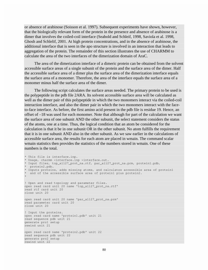
80

or absence of arabinose (Soisson et al. 1997). Subsequent experiments have shown, however, that the biologically relevant form of the protein in the presence and absence of arabinose is a dimer that involves the coiled-coil interface (Seabold and Schleif, 1998, Saviola et al. 1998, Ghosh and Schlelif, 2001. At high protein concentrations, and in the absence of arabinose, the additional interface that is seen in the apo structure is involved in an interaction that leads to aggregation of the protein. The remainder of this section illustrates the use of CHARMM to calculate the area of the two interfaces of the dimerization domain of AraC.

The area of the dimerization interface of a dimeric protein can be obtained from the solvent accessible surface areas of a single subunit of the protein and the surface area of the dimer. Half the accessible surface area of a dimer plus the surface area of the dimerization interface equals the surface area of a monomer. Therefore, the area of the interface equals the surface area of a monomer minus half the surface area of the dimer.

The following script calculates the surface areas needed. The primary protein to be used is the polypeptide in the pdb file 2ARA. Its solvent accessible surface area will be calculated as well as the dimer pair of this polypeptide in which the two monomers interact via the coiled-coil interaction interface, and also the dimer pair in which the two monomers interact with the face-to-face interface. As before, the first amino acid present in the pdb file is residue 19. Hence, an offset of –18 was used for each monomer. Note that although for part of the calculation we want the surface area of one subunit AND the other subunit, the select statement considers the status of the atoms, one at a time. Thus, the logical condition that an atom be considered for the calculation is that it be in one subunit OR in the other subunit. No atom fulfills the requirement that it is in one subunit AND also in the other subunit. As we saw earlier in the calculations of accessible surface area, the results for each atom are placed in wmain. The command scalar wmain statistics then provides the statistics of the numbers stored in wmain. One of these numbers is the total. * This file is interface.inp. * Usage, charmm <interface.inp >interface.out. * Input files, top_all27_prot_na.rtf, par_all27_prot_na.prm, protein1.pdb, * protein2.pdb. * Inputs proteins, adds missing atoms, and calculates accessible area of protein1 * and of the accessible surface area of protein1 plus protein2. * ! Open and read topology and parameter files. open read card unit 20 name "top_all27_prot_na.rtf" read rtf card unit 20 close unit 20 open read card unit 20 name "par_all27_prot_na.prm" read parameter card unit 20 close unit 20 ! Input the proteins. open read card name "protein1.pdb" unit 21 read sequence pdb unit 21 generate pro1 setup rewind unit 21 open read card name "protein2.pdb" unit 22 read sequence pdb unit 22 generate pro2 setup rewind unit 22

81

read coordinate pdb offset -18 unit 21 close unit 21 read coordinate pdb offset -18 append unit 22 close unit 22 ! Add any missing atoms. ic fill preserve ic parameter ic build hbuild ! Calculate and display the surface area of a single protein in isolation. coordinate surface select segid pro1 end accessible scalar wmain statistics ! Calculate and display the surface area of both proteins as a whole. coordinate surface select segid pro1 .or. segid pro2 end accessible scalar wmain statistics stop

The script shown above was applied to the two peptide chains, the peptide whose coordinates are given in 2ARA, and the peptide whose coordinates are obtained by applying transformation four to the given coordinates. The resulting pair engage in the face-to-face interaction. The transformation applied is shown below. REMARK 290 SMTRY1 4 -0.500025 0.865971 0.000000 0.00000 REMARK 290 SMTRY2 4 0.866051 0.500025 0.000000 0.00000 REMARK 290 SMTRY3 4 0.000000 0.000000 -1.000000 0.00000

The following is the relevant output from the script, from which the interface area can be calculated to be I=M-D/2=8013-14025/2=1001 Å2. CHARMM> coordinate surface select segid prot end accessible SELRPN> 2430 atoms have been selected out of 4860 SURFAC: Lennard-Jones radii values being used SURFAC: RPRObe= 1.60000 SURFAC: Analytic surface area method used CHARMM> scalar wmain statistics Statistics for 4860 selected atoms: minimum = 0.00000 maximum = 72.4397 weight = 4860.00 average = 1.64892 variance= 5.83723 total = 8013.76 CHARMM> CHARMM> coordinate surface select segid prot .or. segid pro2 end accessible SELRPN> 4860 atoms have been selected out of 4860 SURFAC: Lennard-Jones radii values being used SURFAC: RPRObe= 1.60000 SURFAC: Analytic surface area method used CHARMM> scalar wmain statistics Statistics for 4860 selected atoms: minimum = 0.00000 maximum = 72.4397 weight = 4860.00 average = 2.88593 variance= 7.49788 total = 14025.6

Performing the same calculations on the dimer pair that interact via the coiled-coil interface yields an area of the interface of 964 Å2. This illustrates the problem that was posed by the

82

structure of the apo form of the protein. The new interface was so large that it seemed likely to be of biological relevance. This proved not to be so, however.

Distance Maps-Secondary Structure Identification in AraC

Contact or energy maps show on a two dimensional lattice the distances or interaction energies between atoms or residues. For example, consider the Cα atoms of residues i and j in a protein that are separated by a distance dist(i, j). The collection of distances where the values of dist(i, j) are placed in the ith row and jth column of a matrix is known as a distance matrix of the protein. While the array of numbers of a distance matrix contains most of the structural the data on a protein, it is difficult to extract much meaning from the mass of numbers. Therefore, instead of placing numbers into the array, cells of the array can be colored, and the resulting patterns can be processed by our very high capacity visual systems to provide an easily interpreted summary of the information. It should be noted that since dist(i, j) = dist(j, i), a distance map is symmetric about the main diagonal from the upper left to the lower right corners. Only half of the matrix needs to be drawn, but we shall construct the full matrix because the presence of symmetry adds visual appeal to the representation.

Consider a single alpha helix. Color those cells of the distance matrix white that contain Cα− Cα distances greater than 8 Å and color them black if they contain a distance less than 8 Å. For the ith residue in an alpha helix, the Cα carbon atoms of only residues i -4, i-3, i-2, i-1, i+1,

Row i

Column j

Figure 2.11 Graphical representation of a distance matrix for an α-helix in which cells containing distances less than 8 Å are colored black. Figure 6.2 A graphical distance matrix for the dimerization domain of AraC protein in which the cutoff distance is 8 Angstroms.

83

i+2, i +3, and i + 4 lie within 8 Å of the Cα atom of the ith residue. Thus, the distance matrix of an alpha helix consists of a strip of black squares down the main diagonal, Fig. 2.11.

Consider two adjacent parallel beta sheet strands. If the first residue of the first strand is residue i, and it is opposite from residue i + n on the second strand, then residue i + 1 is opposite residue i + n + 1 on the second strand and so on. A distance difference map representing this spatial relationship yields two lines black cells on either side of the main diagonal, well offset from it, but parallel to it. Two adjacent antiparallel strands similarly generate two lines of black cells, but these are perpendicular to the main diagonal.

Fig. 2.12 shows a distance matrix for the dimerization domain of AraC protein. Towards the C-terminus at the bottom right is the signature of an alpha helical region. The contacts perpendicular to the main diagonal adjacent to the helical regions shows that the two helical regions are antiparallel to one another. Somewhat before this region another helical region is apparent. More residues are within the 8 Angstrom cutoff distance of this region than in the alpha helical region. Therefore, it is not surprising that this region is also a helix, a 3-10 helix. Earlier in the protein, a prominent antiparallel set of contacts is apparent. The protein is, in fact, folded back upon itself and consists of a very long region of antiparallel contacts that are then wrapped

Figure 2.12 A distance matrix for the dimerization domain of AraC protein.

84

around the arabinose binding pocket. In some areas, three adjacent strands are all within 8 Angstroms of each other. These areas then possess a second strip of black cells parallel to the first.

The following CHARMM commands will calculate the distance matrix between every alpha carbon in a protein and output the result to a file called dist.dmat. open write card name dist.dmat unit 21 coordinate dmat select type ca end select type ca end single unit 21

When applied to the first subunit of AraC 2arc.pdb, this produces the output shown below. ********************************* * DISTANCE MATRIX * NSET1= 161 *** 1=(PROT 7 ASP CA ) *** 2=(PROT 8 PRO CA ) *** 3=(PROT 9 LEU CA ) *** 4=(PROT 10 LEU CA ) *** 5=(PROT 11 PRO CA ) *** 6=(PROT 12 GLY CA ) *** 7=(PROT 13 TYR CA ) *** 8=(PROT 14 SER CA ) *** 9=(PROT 15 PHE CA ) *** 10=(PROT 16 ASN CA ) *** 11=(PROT 17 ALA CA ) *** 12=(PROT 18 HSD CA ) *** 13=(PROT 19 LEU CA ) .. .. *** 158=(PROT 164 MET CA ) *** 159=(PROT 165 GLU CA ) *** 160=(PROT 166 ALA CA ) *** 161=(PROT 167 ILE CA ) ********************************* * NSET2= 161 *** 1=(PROT 7 ASP CA ) *** 2=(PROT 8 PRO CA ) *** 3=(PROT 9 LEU CA ) *** 4=(PROT 10 LEU CA ) .. .. *** 159=(PROT 165 GLU CA ) *** 160=(PROT 166 ALA CA ) *** 161=(PROT 167 ILE CA ) ********************************* * 1 1 0.0000000 1 2 3.8134094 1 3 5.1908672 1 4 5.5314579 1 5 8.1970195 1 6 8.7837469 1 7 6.6315459 .. ..

As shown above, the output lists the atoms that were selected and then lists on one line the identifiers for an atom from each set and the distance between the two atoms. To process the file, it is useful first to remove the identifier lines. This is straightforward since each of these lines, and none of the data lines, contains an asterisk. Grep with the -v option excludes from the output

85

any line containing a string of characters that satisfy the match criterion. The command is shown below. grep -v "*" <file.in >file.out.

The resulting list of distances must be reformatted for importing into a spreadsheet program. The following awk program reads the atom identifiers i and j and places their distance value in a two dimensional array, dist(i, j). In this case, the protein contained 161 residues, and the matrix of distances on the spreadsheet will be 161 by 161. # This file is dmatrix.awk. # Usage, awk -f dmatrix.awk <data.in >file.out. # To extract distances between all pairs in data.in. # and output comma delimited lines suitable for spreadsheet input. # Input data is num1 num2 num3 where num3 is distance between num1 atom and # num2 atom. # Enter the array dimensions in the while loops before running. # Read entire dataset into two dimensional energy array. { dist[$1,$2] = $3 } # At end, print out comma delimited array elements on separate lines END { i=1 j=1 while(i<162) { while(j<162) { printf(dist[i,j], "," ) j++ } printf("\n") j=1 i++ } }

After the array has been filled, which is specified by just a single line in the script, it is printed out row by row in a format suitable for importing into a spreadsheet. Each element in a row must be separated from the next element by a comma so that later the import or open command in the spreadsheet can be instructed to use comma as a column delimiter. At the end of a row of input data, a line return character must be present to instruct the spreadsheet to start a new row. In the awk program, the indices i and j specify which matrix elements to be printed. The print statements output the matrix elements followed by a comma. After an entire line of elements has been printed, the new line character is printed, and output begins on the next line. After importing the data into a spreadsheet program, the cells can then colored black or not, depending on their values, using conditional formatting.

Distance Difference Maps, Application to Hemoglobin

A distance difference map is related to a distance map. These useful maps reveal the structural differences between two conformations of a protein. The distance difference matrix contains the change in the separation distance of residues between two conformational states. Residue pairs whose separation distance remains the same in the two conformational states have

86

a distance difference of zero and can be represented as white cells. The larger the distance difference between a pair of residues in the two conformations, the darker one can color the matrix element. Residues that move with respect to the rest of the protein are then revealed by horizontal and vertical bands of dark cells.

A matrix of distance differences in a spreadsheet can be produced by generating two distance matrix spreadsheets and then subtracting one from the other. Once a matrix of distance differences has been created, the following Visual Basic script will colorize the cells according to their values. This more complicated method of colorizing the cells is necessary because conditional formatting, as used in the previous section, is unable to handle more than three conditions. As there is then no way to lock in colors that have been chosen, conditional formatting is inadequate for refined uses. To use this script, under the Tools-Macro menu item in the spreadsheet create a new macro called DistMatrix, and then paste the following script into the Visual Basic editor which opens. From the spreadsheet, run the macro DistMatrix. 'For coloring cells of Excel spreadsheet by values they contain. 'Handles up to 230 x 230 matrix. 'Copy values into spreadsheet, set appropriate limits in case statements below. 'Run spreadsheet Macro DistMatrix. 'Adjust row heights and column widths. Sub DistMatrix() 'Declare Constants and variables Dim ColNo As Integer Dim RowNo As Integer ' Set six palette colors and clear colors from sheet ActiveWorkbook.Colors(1) = RGB(255, 0, 0) 'Dark red ActiveWorkbook.Colors(2) = RGB(255, 150, 150) 'Medium red ActiveWorkbook.Colors(3) = RGB(255, 215, 215) 'Light red ActiveWorkbook.Colors(4) = RGB(215, 215, 255) 'Light blue ActiveWorkbook.Colors(5) = RGB(150, 150, 255) 'Medium blue ActiveWorkbook.Colors(6) = RGB(0, 0, 255) 'Dark blue ActiveSheet.Range("A1", "IV65536").Interior.ColorIndex = xlNone 'Cycle through matrix area. For RowNo = 1 To 230 For ColNo = 1 To 230 'Case statement obtains value of cell(i,j), and if it is in the range ' indicated, sets color index of the cell appropriately Select Case Cells(RowNo, ColNo).Value Case -10 To -2 Cells(RowNo, ColNo).Interior.ColorIndex = 6 Case -2 To -1 Cells(RowNo, ColNo).Interior.ColorIndex = 5 Case -1 To -0.5 Cells(RowNo, ColNo).Interior.ColorIndex = 4 Case 0.5 To 1 Cells(RowNo, ColNo).Interior.ColorIndex = 3 Case 1 To 2 Cells(RowNo, ColNo).Interior.ColorIndex = 2 Case 2 To 10 Cells(RowNo, ColNo).Interior.ColorIndex = 1 End Select Next ColNo Next RowNo Erase values, leaving just the colored backgrounds. ActiveSheet.Range("A1:IV256").ClearContents End Sub

87

Hemoglobin significantly changes conformation between the deoxy, T, and the oxy, R, states. Thus, this is a good subject for a distance difference map. Fig. 2.13 shows such a map, constructed as described above from the pdb coordinates of deoxy hemoglobin, 2HHB and from oxy hemoglobin, 1HHO, where the N-terminus of the α1 subunit is located at the upper left corner. In this map the darkest colors represent the greatest distance changes and lighter colors,

Figure 2.13 A graphical distance difference matrix for the tetrameric hemoglobin between the deoxy and oxy states in which the subunits are labeled α1, β1, α2, and β2. The darkest colors represent distance change greater than 4 Angstroms, medium color represents distance changes between 1 and 4 Angstroms, and the lightest color represents changes between 0.4 and 1 Angstroms. No color is used for smaller changes. Blue is used for decreases in distance, and red for increases in distance.

88

smaller changes. CHARMM required less than a minute to generate the list of distances used in the map’s construction. The spreadsheet program, however, could not handle the entire distance matrix at once, and therefore the figure was constructed in parts.

The map shows a number of well known features in hemoglobin's conformational changes. The upper left hand square, α1 x α1, represents the distance changes within the α1 subunit. The rather prominent band two thirds of the distance to the C-terminus of the α1 subunit derives from movement of the F helix. Histidine 87 of this helix contacts the Fe atom in the heme group, and changes in the radius of the iron move the histidine that then drives the conformational changes in the protein. Similar changes occur in the β subunit as shown in the β1 x β1 matrix or the β2 x β2 matrix. The C-terminus of this subunit also shows a substantial movement. As a whole, there is not a lot of movement of α1 with respect to β1 or of α2 with respect to β2 as shown by the overall lightness of areas representing these motions, the upper left and the lower right sets of four squares. By far the largest motions occur between the α1β1 pair and the α2β2 pair as shown by the darkness of the α1β1 x α2β2 and α2β2 x α1β1 areas of the matrix.

The subunits of hemoglobin primarily rotate in going from the deoxy to the oxy state. This can be seen using the coordinate orient command. The four subunits of deoxy hemoglobin, and the four subunits of oxy hemoglobin were loaded into CHARMM, and the oxy hemoglobin was reoriented with coordinate orient so as to overlay its α1 subunit on the deoxy α1 subunit. Then the amount of translation and rotation necessary to overlay each of the remaining three oxy conformation subunits on the corresponding deoxy conformation subunits was determined by again using the coordinate orient command. The relevant commands for this second overlaying operation are given below for the β1 subunits, whose segment id's were DEB1 and OXB1. coordinate copy comparison select all end coordinate comparison duplicate select segid DEB1 end select segid OXB1 end coordinate orient rms select segid OXB1 end

The commands above generated the following output. CHARMM> coordinate copy comparison select all end SELRPN> 17532 atoms have been selected out of 17532 SELECTED COORDINATES COPIED TO THE COMPARISON SET. CHARMM> CHARMM> coordinate comparison duplicate select segid DEB1 end select segid OXB1 end SELRPN> 2241 atoms have been selected out of 17532 SELRPN> 2241 atoms have been selected out of 17532 CHARMM> CHARMM> coordinate orient rms select segid OXB1 end SELRPN> 2241 atoms have been selected out of 17532 CENTER OF ATOMS BEFORE TRANSLATION 13.26180 -8.15701 8.89587 CENTER OF REFERENCE COORDINATE SET 14.05806 -8.36168 9.88076 NET TRANSLATION OF ROTATED ATOMS 0.79627 -0.20467 0.98489 ROTATION MATRIX 0.998291 0.049222 -0.031492 -0.049931 0.998507 -0.022153 0.030355 0.023688 0.999258 AXIS OF ROTATION IS -0.365182 0.492688 0.789874 ANGLE IS 3.60 TOTAL SQUARE DIFF IS 7270.3325 DENOMINATOR IS 2241.0000

89

THUS RMS DIFF IS 1.801176 ALL COORDINATES ORIENTED IN THE MAIN SET BASED ON SELECTED ATOMS.

The above output shows that the β1 subunit moved 1.28 Angstroms,

( ) ( ) ( )222 985.0205.0796.0 +−+ , and rotated 3.6 degrees with respect to the α1 subunit as the

hemoglobin changed from the deoxy to the oxy state. Similar output showed that the α2 subunit moved 3.4 Angstroms and rotated 13.6 degrees with respect to the α1 subunit, and that the β2 subunit moved 4.3 Angstroms and rotated 12.6 degrees. These numbers reflect the same conclusion as is visually obvious in the distance difference matrix, that there was little movement of β1 with respect to α1, that is, the α1 and β1 subunits behave largely as a unit, as did the α2 and β2 subunits, but that the two units moved significantly with respect to each other.

90

Problems

1. Modify the fixpdb.awk script to generate from a pdb file a single line containing the one letter amino acid abbreviations for the sequence of the residues contained in the pdb file.

2. For a protein like AraC, pdb identification label 2ARC, extract chain A with fixpdb.awk and then delete one, and then both, of the C-terminal oxygen atoms and use the resulting files for input to CHARMM.

3. Overlaying one of the dimerization domains of AraC containing bound arabinose, 2ARC.PDB with one of the dimerization domains containing bound fucose, 2AAC.PDB, an arabinose analog, gave an odd result. To explore the cause, write a CHARMM script that will compute the distance between each pair of Ca atoms for residues 7-166 in a protein, and run on each of the proteins. Next, write an awk script that will extract and sum together these distances. What do your results mean? By the way, x-ray crystallographers say this should not happen.

4. Prepare 2ARC.PDB for input to CHARMM, output the coordinates in pdb format and examine the structure with a molecular display program. Manually delete the side chain atoms of several of the leucine residues in the input pdb file and let CHARMM rebuild the missing atoms and examine the rebuilt protein. Why, in general, do positions of the rebuilt side chain atoms differ from their original positions?

5. What happens when the final return character is omitted from a pdb file that is used as input to CHARMM?

6. Extract and plot the omega angles of the dimerization domain of AraC found in 2ARC.

7. Determine the residues in the dimerization domain of AraC that contact Arg38.

8. Use CHARMM to generate a file containing the internal coordinates of the dimerization domain of AraC. Use awk to set the omega angles of the peptide bond to 180° or 0°, whichever is closer. Read these back into CHARMM and rebuild the protein with these very slightly altered backbone angles. Examine the structure with a molecular display program. How does this structure compare with the actual structure?

9. Pick from the Protein Data Bank a dozen or so globular proteins of widely different molecular weight. Make a plot of the fraction of interior residues, say those with less than 15% of their surface area exposed to solvent, as a function of molecular weight.

10. In order that distance matrices and distance difference matrices not be hopelessly complex jumbles of light and dark squares, what general distance property must exist between residues in proteins?

11. Why does the overlay script not include the backbone atoms HN and HA?

Bibliography

Adzhubei, A. and Sternberg, M. (1993). Left-handed Polyproline II Helices Commonly Occur in Globular Proteins, J. Mol. Biol. 229, 472-493.

91

Berman, H. M., Westbrook, J., Feng, Z., Gilliland, G., Bhat, T. H., Weissig, H., Shindyalov, I. N., and Bourne, P. E. (2000). The Protein Data Bank, Nucleic Acids Research, 28, 235-242.

Ghosh, M. and Schleif, R. (2001). Biophysical Evidence of Arm-Domain Interactions in AraC, Anal. Biochem. 295, 107-112.

Gorodkin, J., Stærfeldt, H. H., Lund, O., and Brunak S. (1999). MatrixPlot: Visualizing Sequence Constraints.Bioinformatics 15:769-770, 1999.

Hovmöller, S., Zhou, T., and Ohlson, T. (2002). Conformations of Amino Acids in Proteins, Acta Crystallographica D58, 768-776.

Lee, B. and Richards, F. M. (1971). The Interpretation of Protein Structures: Estimation of Static Accessibility, J. Mol. Biol. 55, 379-400. Not only defines accessible surface area, but also gives an idea of the methods by which early investigators operated without powerful personal computers.

Ramachandran, G. N. and Sasiskharan V. (1968). Conformation of Polypeptides and Proteins, Adv. Protein Chem. 23, 283-437. A classic and widely cited paper.

Richards, F.M., and Kundrot, C.E. (1988). Identification of Structural Motifs From Protein Coordinate Data: Secondary Structure and First Level Super-Secondary Structure, Proteins 3, 71-84.

Richmond, T. J. and Richards, F. M. (1978). Packing of α-Helices: Geometrical Constraints and Contact areas, J. Mol. Biol. 119, 537-555.

Srinivasan, R., and Rose, G. (1994). The T-to-R Transformation in Hemoglobin: A Reevaluation, Proc. Nati. Acad. Sci. USA 91, 11113-11117. SE

Saviola, B., Seabold, R., and Schleif, R. (1998). Arm-Domain Interactions in AraC, J. Mol. Biol. 278, 539-548.

Seabold, R., and Schlelif, R. (1998). Apo-AraC Actively Seeks to Loop J. Mol. Biol. 278, 529-538.

Soisson, S., MacDougall-Shackleton, B., Schleif, R., and Wolberger, C. (1997). Structural Basis for Ligand-Regulated Oligomerization of AraC, Science, 276, 421-425.

Related Web Sites

http://www.rcsb.org/pdb/index.html Protein Data Bank

http://www-106.ibm.com/developerworks/library/l-awk1.html Common threads: Awk by example, Part 1. An intro to the great language with the strange name.

http://www-106.ibm.com/developerworks/library/l-awk2.html Common threads: Awk by example, Part 2. Records, loops, and arrays

92

http://www-106.ibm.com/developerworks/library/l-awk3.html Common threads: Awk by example, Part 3. String functions and ... checkbooks?

http://sparky.rice.edu/~hartigan/awk.html Many examples of awk usage.

http://www.netsci.org/Science/Compchem/feature14.html Molecular Surfaces: A Review. In fact a wonderful review by Michael Connolly, one of the pioneers in computation of molecular surfaces.

http://www.netsci.org/Science/Compchem/index.html Computational Chemistry. A site with a number of articles on computational chemistry, including several on molecular surfaces.

http://www.rcsb.org/pdb/biounit_tutorial.html A tutorial on asymmetric units, unit cells, and biomolecules.

http://www.ks.uiuc.edu/Research/vmd/ Website for VMD containing the program, documentation, scripts, images, and examples.

http://www.cbs.dtu.dk/services/MatrixPlot/distmatr/index.html/ A site for the convenient generation of distance and distance difference matrices. Data from the dmat matrix output from CHARMM is easily reformatted for submission to this site which will then return a postscript file of the matrix map.

93

Chapter 3

Energy Minimization and Running Dynamics Simulations The previous chapter concerned the extraction of information from existing coordinates. That is, geometric properties of static proteins were considered. In this chapter, atoms will be allowed to move with respect to one another. First, in energy minimizing a structure or system, positions of atoms are allowed to shift so as to bring the system energy to a lower value. Often such adjustments are very small and merely accommodate the slightly different atomic radii as used by protein crystallographers and by CHARMM. Sometimes however, they can be quite large if we are moving parts of proteins around by pushing or pulling on them with artificially imposed forces. The second source of movement is performing a molecular dynamics simulation. In such simulations atoms are given velocities appropriate to a chosen temperature and allowed to move in response to all the forces acting on them in paths determined by Newton's equations of motion. The study of the movements of proteins in molecular dynamics simulations may give more correct or more useful information about the structure and function of proteins than an examination of static structures. Whether or not such studies can provide deep insights to protein function remains to be learned, but such studies clearly provide information about the motions and behavior of portions of proteins that range in size from side chains to domains.

Methods of Energy Minimization

An energy minimum is found by moving each atom down the potential until each is at a point where the energy can no longer be reduced by small movements or where the gradient of the potential with respect to changes in the atom's coordinates, force, is zero(minimiz.doc). Over the years of CHARMM’s development, six different mathematical methods for minimizing a function of many variables have been applied to molecular systems. These differ in their stability, ability to reach a minimum, suitability when a system is far from a minimum, and speed of convergence. In general, however, for the problems considered in this book, the adopted basis Newton-Raphson, ABNR method is the best general purpose choice.

The forces acting on each atom derive from its covalent bonds and from the two forces that act at a distance, the Van der Waals forces and electrostatic forces. As described earlier, to economize on the number of calculations that must be made to calculate the nonbonded forces, a nonbonded list (nbonds.doc) is maintained. It lists for each atom those other atoms that must be used in the calculation of the nonbonded forces. The criteria for membership on the list and details of the calculations are contained in the nonbonded specifications. Default parameters of the nonbonded list are contained in the parameter file and are used automatically if no others are explicitly provided. In most cases, the parameters provided in the parameter table are appropriate. As the accuracy and success of simulations depends on these values, they should, however, be examined for suitability to the problem. Below is shown part of the documentation on minimization by CHARMM. MINI ABNR [ nonbond-spec ] [ hbond-spec ] – [ INBFrq 0 ] [ IHBFrq 0 ] – [NOUPdate] [STEP real] [GRADient] [DEBUg] - [ frequency-spec ] [ tolerence-spec ] [ print-spec ] - { ABNR abnr-spec }

94

Where nonbond-spec is described in nbonds.doc hbond-spec is described in hbonds.doc frequency-spec::= [NSTEP int] [IHBFrq int] [INBFrq int] [NPRInt int] tolerence-spec::= [TOLENR real] [TOLGRD real] [TOLITR int] [TOLSTP real] print-spec::= [IMAXp int] [IPRInt int] [PRTMin int] abnr-spec::= [EIGRng real] [MINDim int] [STPLim real] - [STRIct real] [ MASS ] [PSTRct real] [LATTice] [NOCOordinates] [FMEM real]

Many details of the way an energy minimization can be specified. For the most part, these details are of interest only to experts concerned with the details of the computations and we may safely bypass them. Thus, it is usually necessary only to specify the desired number of steps of energy minimization with the nstep parameter and the frequency at which the energies are printed to the output with the nprint parameter.

Energy Minimizing the Dimerization Domain of AraC

This section illustrates a script for the energy minimization of the dimerization domain of AraC and displays some of the output that is generated during such a minimization. The pdb file 2ARC.pdb must first be processed by awk using the fixpdb.awk file to extract one subunit, assign the name prot to the polypeptide chain, and generate the file protein.pdb that is suitable for input to CHARMM. The command is. awk –f fixpdb.awk segid=prot chainID=A <2ARC.pdb >protein.pdb

The following script reads CHARMM’s topology and parameter files, generates coordinates for missing atoms, centers the protein at the origin, and performs 1000 steps of energy minimization, printing a summary of the results each 20 steps. Problems at the end of the chapter illustrate that in this case, atoms may be shifted by as much as several Angstroms, but that a characteristic movement is on the order of 0.5 Angstrom. * This file is mini.inp. * Usage, charmm <mini.inp >mini.out. * Input files, top_all27_prot_na.rtf, par_all27_prot_na.prm, protein.pdb from * fixpdb.awk. * Reads protein.pdb, adds H atoms, adds missing side chain atoms, centers at * origin and orients major axis along x axis. * Energy minimizes * ! Open and read topology and parameter files. open read card unit 20 name "top_all27_prot_na.rtf" read rtf card unit 20 close unit 20 open read card unit 20 name "par_all27_prot_na.prm" read parameter card unit 20 close unit 20 ! Read in protein, prepare internal arrays, build missing coordinates. open read unit 21 card name "protein.pdb" read sequence pdb unit 21 generate prot setup rewind unit 21

95

read coordinate pdb offset -6 unit 21 close unit 21 ic fill preserve ic parameter ic build hbuild ! Center protein at the origin. coordinate orient ! Energy minimize mini abnr nstep 1000 nprint 20 ! Write outputs open write unit 30 card name prot.pdb write coordinates pdb select all end unit 30 * Coordinates of all atoms in protein, pdb format * system - "echo Script ran without crashing > /dev/tty" stop

The coordinate orient command places the center of mass of the protein at the origin and rotates the molecule so that principle geometric axis is along the x-axis and the next largest is along with the y-axis. The output displays information concerning the translation and rotation that is performed. CHARMM> ! Center protein at the origin CHARMM> coordinate orient ORIENT THE COORDINATES TO ALIGN WITH AXIS MOMENTS 154571.98081436 -19241.03804083 18203.77790833 262614.15908356 -19469.12705103 173065.57712500 Transpose of the rotation matrix 0.225476 -0.954959 0.192909 0.843063 0.290488 0.452616 -0.488267 0.060581 0.870589 CENTER OF ATOMS BEFORE TRANSLATION 17.13913 36.24537 40.24876 AXIS OF ROTATION IS 0.199785 -0.347134 -0.916288 ANGLE IS 78.86 ALL COORDINATES ORIENTED IN THE MAIN SET BASED ON SELECTED ATOMS.

The command to minimize the energy of the system produces the following output. As we have not explicitly provided values for the nonbonded list, they are taken from the parameter table and displayed. The parameters governing the minimization are also displayed. They include the two we specified plus a number of other default values. At the beginning of an energy minimization, it is not unusual to see warnings concerning some improper dihedral angles. If these do not disappear shortly or appear later in the minimization or dynamics run, something is wrong, perhaps a residue is misdefined. The various energies are reported in the table that follows. Note the very large positive initial energy of the system.

96

CHARMM> CHARMM> mini abnr nstep 1000 nprint 20 NONBOND OPTION FLAGS: ELEC VDW ATOMs CDIElec SHIFt VATOm VSWItch BYGRoup NOEXtnd NOEWald CUTNB = 14.000 CTEXNB =999.000 CTONNB = 10.000 CTOFNB = 12.000 WMIN = 1.500 WRNMXD = 0.500 E14FAC = 1.000 EPS = 1.000 NBXMOD = 5 There are 0 atom pairs and 0 atom exclusions. There are 0 group pairs and 0 group exclusions. <MAKINB> with mode 5 found 7431 exclusions and 6862 interactions(1-4) <MAKGRP> found 2404 group exclusions. Generating nonbond list with Exclusion mode = 5 == PRIMARY == SPACE FOR 749413 ATOM PAIRS AND 0 GROUP PAIRS == PRIMARY == SPACE FOR 1124139 ATOM PAIRS AND 0 GROUP PAIRS General atom nonbond list generation found: 828614 ATOM PAIRS WERE FOUND FOR ATOM LIST 43973 GROUP PAIRS REQUIRED ATOM SEARCHES ABNER> An energy minimization has been requested. EIGRNG = 0.0005000 MINDIM = 5 NPRINT = 20 NSTEP = 1000 PSTRCT = 0.0000000 SDSTP = 0.0200000 STPLIM = 1.0000000 STRICT = 0.1000000 TOLFUN = 0.0000000 TOLGRD = 0.0000000 TOLITR = 100 TOLSTP = 0.0000000 FMEM = 0.0000000 MINI MIN: Cycle ENERgy Delta-E GRMS Step-size MINI INTERN: BONDs ANGLes UREY-b DIHEdrals IMPRopers MINI EXTERN: VDWaals ELEC HBONds ASP USER ---------- --------- --------- --------- --------- --------- MINI> 0 9899.52281 0.00000 199.91051 0.00000 MINI INTERN> 230.66281 3382.13205 1659.89723 701.37550 12.60637 MINI EXTERN> 7095.10693 -3182.25809 0.00000 0.00000 0.00000 ---------- --------- --------- --------- --------- --------- UPDECI: Nonbond update at step 14 Generating nonbond list with Exclusion mode = 5 == PRIMARY == SPACE FOR 1124139 ATOM PAIRS AND 0 GROUP PAIRS General atom nonbond list generation found: 828117 ATOM PAIRS WERE FOUND FOR ATOM LIST 43857 GROUP PAIRS REQUIRED ATOM SEARCHES MINI> 20 -1603.09005 11502.61287 5.15236 0.59575 MINI INTERN> 197.30435 1153.02572 297.04947 793.64587 19.55582 MINI EXTERN> -511.51241 -3552.15888 0.00000 0.00000 0.00000 ---------- --------- --------- --------- --------- ---------

The output data is presented in a format of three header lines defining various terms followed by three lines of data corresponding to the terms above. The first row refers to general properties of the system and the progress of the minimization. GRMS is the root mean square of the gradients of the potential energy with respect to variation of each of the coordinates of each atom in the system.

97

At an energy minimum, GRMS should be close to zero. The HBONds term is zero as it should be because hydrogen bonding in CHARMM is now accounted for by other energy terms. ASP refers to an energy term that is not used here that depends upon the area of the surface that is accessible to the solvent. USER refers to a user defined energy term.

By step 1000 of the minimization we see that the total energy, the change in energy since the last printout, the GRMS, and the step size, have all become much smaller than they were initially. Of course, as an energy minimum is approached, the change in energy and the GRMS must become smaller. The reduction in step size is a feature of the ABNR minimization algorithm, which allows large steps to be taken while the system is far from a minimum, and then reduces the step size as the minimum is approached. ABNR MIN: Cycle ENERgy Delta-E GRMS Step-size ABNR INTERN: BONDs ANGLes UREY-b DIHEdrals IMPRopers ABNR EXTERN: VDWaals ELEC HBONds ASP USER ---------- --------- --------- --------- --------- --------- ABNR> 1000 -4007.56101 5.63910 0.35970 0.01450 ABNR INTERN> 168.12958 475.16113 43.42465 747.13789 17.10833 ABNR EXTERN> -642.67941 -4815.84319 0.00000 0.00000 0.00000 ---------- --------- --------- --------- --------- ---------

Considerations for a Dynamics Simulation

An accurate simulation of the motions of each atom in a protein necessitates using time steps short in comparison to the highest atomic oscillation rate. If this requirement is not met, in a time step, an atom could move from a point where its interaction energy with another atom is negligible to having penetrated far inside a Van der Waals radius where its interaction energy could be enormous, Fig. 3.1. Conversion of this high potential energy into kinetic energy as the atom is repulsed, will give it a similarly tremendous velocity. Shortly, in a single time step, such a high velocity atom will deeply penetrate the Van der Waals potential of another atom, and the

∑ =

∂ ∂ = N

i i x U

N GRMS 3 1

2 3 1

Initial

One time step later

Two time steps later

Figure 3.1 Interpenetration followed by violent repulsion when time step is too large.

98

entire system will soon “explode”. Hydrogen atoms vibrate the most rapidly, and their motion necessitates that a time step in a dynamics simulation be on the order of a femtosecond or less. Thus, on the order of a million time steps must be used merely to simulate a system for a nanosecond. Since many of the activities of proteins are thought to require times from nanoseconds to beyond milliseconds, and the systems being simulated often consist of a hundred thousand or more atoms, much of the effort of the molecular dynamics experts has been directed towards finding simulation procedures that maximize computational efficiency and minimize the computational power required. This effort to maximize the quality of numerical results obtained has spawned a huge number of simulation possibilities and a bewildering array of options. The objective of this section of the book is not to explore the intricacies of these possibilities, but rather to show how simple simulations may be set up and the results analyzed. Before returning to this theme, it is necessary to discuss however, the parameters of importance in most simulations and to mention a few of the more commonly encountered refinements.

One frequently used approximation is to constrain the lengths of the bonds to hydrogen atoms and then to calculate the positions of hydrogen atoms without dynamics considerations. Although these calculations somewhat lengthen the time required to calculate new coordinate positions, the size of a time step can be increased from 0.0005 to 0.001, and the overall effect is a considerable increase in the effective speed of the calculation. Doubling the step length effectively doubles the computation speed since almost the same number of steps yields a

Figure 3.2 Two dimensional periodic boundary conditions. The central square is surrounded by eight image squares. A particle leaving one square enters another.

99

simulation for twice as long. The command for constraining hydrogen bonds is shake bonh (cons.doc).

One issue of concern in simulations is the possibility of anomalous effects generated by boundaries between a protein plus the water molecule in which it is immersed and the rest of empty space, the surrounding vacuum. Since real molecules in solution are very far from boundaries, it makes sense to perform simulations in which all boundaries have been removed. Periodic boundary conditions eliminate boundary effects, essentially by surrounding the molecule with space filling images of itself. This is done by mapping the edges of the volume being simulated back onto itself. In cubical geometry this is done by simulating the central cube and considering the surrounding cubes, 26 in all, as identical images of the central cube. A number of different geometries completely fill space and can be used for calculations using periodic boundary conditions. These include cubes, rhomobohedra, rhombic dodecahedra, truncated octahedra, and hexagonal prisms. When an atom or molecule passes out of the central cell for cubical geometry, for example, by moving past the right boundary, it enters the right hand image box from the left, Fig. 3.2. Of course, this same event happens in every one of the images of the central box. Additionally then, an image of the atom or molecule also enters the central box from the left. By these means no boundary exists, and surface effects are eliminated, but at the expense of increased computational load and occasional artifacts arising from the existence of images and interactions between image molecules and “real” molecules. The use of periodic boundary conditions is generally considered to best represent reality and many simulations are performed using periodic boundary conditions.

Table 3.1 shows the major types of systems that can be simulated with CHARMM. Many of the examples presented in this book do not use periodic boundary conditions as the problems being considered do not require such sophistication. Instead, proteins will be immersed in droplets of water. After an example of a protein in a water drop, an example using periodic boundary conditions will be given. Finally, a simulation will be done in which no water molecules are present at all. This, of course, represents reality less well than having water present even though special parameter and topology tables have been devised to compensate for the absence of explicit water molecules. A virtue of eliminating the explicit water molecules and using implicit water is that calculations are much faster.

Table 3.1 Types of Systems Simulated by CHARMM System Comments

Constant energy, constant number No boundary Constant temp., constant number Periodic boundary conditions

Constant pressure, constant number Periodic boundary conditions Constant energy, constant volume, constant number Fixed periodic boundary conditions Constant temp., constant volume, constant number Fixed periodic boundary conditions Constant pressure, constant temp, constant number Periodic boundary conditions

Langevin simulation Atoms obey Langevin equation Stochastic boundary conditions Hybrid of Langevin and constant

energy

100

Once a system is fully defined, it seems like it should be possible to start from a known structure of a protein, set the atoms in motion and follow their positions over time, that is, to run the dynamics. In practice, this is not possible because in the structure determination some atoms will almost surely have been placed such that their bonds are stretched or such that they slightly overlap other atoms. If the dynamics were begun from such a state, these atoms could feel impossibly large forces and would accelerate to velocities outside the range that can be handled by CHARMM. To prevent this problem, before the dynamics are started, a system is brought to a state where the sum of forces acting on each atom is nearly zero. Since the net force acting on an atom is given by the derivative or gradient of the potential with respect to changes in the position of that atom, the desired position is one where all the derivatives are zero. Since the system is "smooth", such a point is an energy minimum or energy maximum of the system. In fact, it is an energy minimum. Therefore, before a dynamics simulation can be run, an energy minimization needs to be performed.

Starting a dynamics run with every atom at rest and every atom initially feeling a net force of zero is equivalent to starting the system at absolute zero. One of the main reasons, however, for doing molecular dynamics is permit study of systems under normal conditions. Thus, an energy minimized system needs to be warmed up to about 300 degrees Kelvin. In some cases it is possible to assign each atom a velocity near the value characteristic for an atom of that mass at 300 degrees and let the system evolve in time thereafter. Sometimes, however, this approach leads to the development of intolerable instabilities and CHARMM automatically stops the simulation. Therefore, usually systems are brought to the desired temperature by gradually incrementing each atom's velocity and then allowing time for this perturbation to die away before the next velocity increment. Often, systems are not completely equilibrated after these heating steps, and further evolution in the absence of heating is needed. Ordinarily the system then comes to equilibrium at a temperature slightly different from what is desired. After a further period of equilibration, the velocities are scaled so as to yield the desired target temperature. This process of equilibration followed by velocity scaling is performed until the system temperature remains constant at the desired value. Then the system is allowed to evolve in the absence of velocity adjustments. This is called the simulation or production phase.

Many additional parameters can be adjusted to control the heating, equilibration, and simulation phases of a dynamics run (dynamc.doc). These include choices on the method of integration, the size of the time step to be used, number of steps, the input and output files to be used, parameters controlling heating or equilibration, the frequencies of incrementing or adjusting velocities and of outputting information, the way that velocities are incremented, and the temperature limits. These can be categorized as shown in Table 3.2.

To reduce the impact of a power outage or a system malfunction during a long molecular dynamics run, restart files can be periodically written. These contain atom positions and velocities and permit the system to be restarted from the state of the system at the time the restart file was written. During the simulation phase, energy in a system should be conserved and starting total energy should be close to the final total energy term. Small fluctuations in temperature and a slow rise in the average temperature are normal, but increases in temperature of five to ten degrees in a thousand steps indicate that the system is unstable and soon the calculation will crash. Such instabilities can sometimes be forestalled by slower heating and more extensive equilibration or by stopping and equilibrating the temperature before proceeding.

101

Another criterion for a successful simulation is that the ratio of the RMS fluctuation of the total energy to the RMS fluctuation of the kinetic energy should not be much larger than 0.001. In the literature one can find very elaborate protocols that sometimes are followed for equilibrating systems. How these were devised and whether they are necessary is rarely described, however. After the molecular system has been equilibrated, a short trajectory of free dynamics should be run to determine the stability of the energy and the temperature.

Several refinements are commonly encountered in simulations utilizing periodic boundary conditions. One of these is the Ewald approximation (ewald.doc). The Ewald method solves the problem that is generated in simulations with periodic boundary conditions from the fact that the strength of an electric field generated by a charge diminishes with the square of the distance from the charge, but the number of images containing a charge increases as the square of the distance. Another refinement is coupling the system to a thermal reservoir so as to maintain temperature (nose.doc), or maintaining a constant pressure by allowing one or more of the walls of the main cell to move (pressure.doc). CHARMM can be instructed to use these refinements by the inclusion of a few keywords and parameter values in the dynamics command. Typical values are provided in the documentation on these three methods.

A Dynamics Run with the AraC Dimerization Domain

In this section a complete script will be given for immersing the dimerization domain of AraC in a droplet of water, energy minimizing, and then heating, equilibrating, and running production dynamics. The steps to be performed are indicated in Fig. 3.3. The protein data bank file of the protein, 2ARC.pdb contains both subunits of the protein as well as a large number of crystallographic water molecules. Those which are close to one of the subunits will be kept. In addition, a box of water molecules whose construction is described in the modeling chapter, is added. This is centered around the protein and crystallographic water molecules, and all of its molecules whose oxygen atoms lie within 2.5 Angstroms of either the protein or crystallographic water molecules are deleted as well as water molecules whose oxygen atoms lie more than 8 Angstroms from the protein.

The two commands shown below extract one subunit from 2ARC.pdb into protein.pdb and the crystallographic water molecules into xwater.pdb, and the CHARMM script for performing the dynamics follows.

Table 3.2 Categories of Dynamics Parameters Category Specifics Method Simulation type and integration method Steps Step number and size

Input and Output Units Input and output files to be used and unit numbers Temperature Temperature and heating specifications Frequency Frequencies for adjusting average velocity,

temperature, heating, writing various outputs Additional How velocity is assigned or scaled

102

awk -f fixpdb.awk segid=prot chainID=A <2ARC.pdb >protein.pdb awk -f fixpdb.awk segid=xwat resname=HOH <2ARC.pdb >xwater.pdb

Initial PDBcoordinate file

Protein coordinates

Remove alternativeconformations

HIS to HSDILE CD1 to CD

O or OCT1 to OT1Provide segid PROT

Add missing atomsAdd hydrogens

Bound watercoordinates

HOH to TIP3O to OH2

Provide segid SOLV

Box of water

Recenter box of water atorigin. Remove overlapping

waters.

Energy Minimize

Run dynamics

Combine, center proteinand crystallographic

waters at origin

Awk with fixpdb script

Figure 3.3 Operations performed by awk and CHARMM in preparing for a dynamics run on a protein.

103

* This file is mindyn.inp. * Usage, charmm <mindyn.inp >mindyn.out. * For putting a protein and its crystallographic waters in a water drop * energy minimizing, heating, equilibrating, and performing a dynamics run. * Takes nonbonded parameters from parameter table. * ! Open and read amino acid topology and parameter files. open read card name "top_all27_prot_na.rtf" unit 20 read rtf card unit 20 close unit 20 open read card name "par_all27_prot_na.prm" unit 20 read parameter card unit 20 close unit 20 ! Read sequences and coordinates from the pdb and crd files. open read card name "protein.pdb" unit 21 read sequence pdb unit 21 generate prot setup rewind unit 21 open read card name "xwater.pdb" unit 22 read sequence pdb unit 22 ! Could also be read sequence TIP3 n unit 22 where n is number of waters in file. generate xwat setup first none last none noangle nodihedral rewind unit 22 open read card name "box.crd" unit 23 read sequence TIP3 4096 unit 23 generate box setup first none last none noangle nodihedral rewind unit 23 read coordinate pdb offset -6 unit 21 close unit 21 read coordinate pdb append unit 22 close unit 22 read coordinate card append unit 23 close unit 23 ! Add missing atoms. ic fill preserve ic parameter ic build hbuild system - "echo Finished adding atoms > /dev/tty" ! Delete crystallographic waters more than 8 Angstroms from the protein. delete atom select ( .byres. ( .not. ( segid prot .around. 8 ) .and. - (segid xwat .and. type OH2 ) ) ) end ! Center protein & crystal. waters at origin. Note, use .or., not .and. coordinate orient select segid prot .or. segid xwat end ! Reverse rotating effect of coordinate orient on the water box. coordinate rotate XDIR ?XAXI YDIR ?YAXI ZDIR ?ZAXI PHI -?THET select segid box end ! Reverse translation effect of coordinate orient on the water box. coordinate translate select segid box end XDIR -?XMOV YDIR -?YMOV ZDIR -?ZMOV ! Delete waters of box that overlap the protein. delete atom select ( .byres. ( (segid prot .around. 2.5 ) .and. - (segid box .and. type OH2 ))) end

104

! Delete waters of box too far from the protein. delete atom select ( .byres. ( .not. (segid prot .around. 10 ) .and. - (segid box .and. type OH2 ))) end ! Delete waters of box that overlap crystallographic waters. delete atom select ( .byres. ((segid xwat .around. 2.5 ) .and. - (segid box .and. type OH2 ))) end ! Change the segid of all water molecules to solv. join xwat box renumber rename segid solv select segid xwat end open write card name ready.pdb unit 40 write coordinates pdb select all end unit 40 * Coordinates after centering of all atoms in protein, pdb format * system - "echo Starting minimization > /dev/tty" minimize abnr nstep 1000 nprint 100 open write card name "heat.rst" unit 31 open write file name "heat.dcd" unit 32 system - "echo Started heating > /dev/tty" ! Heating dynamics dynamics leap verlet strt - nstep 6000 timestep 0.001 nprint 500 nsavc 100 - nsavv 0 inbfrq -1 iprfrq 100 ihtfrq 200 - iunrea -1 iunwri 31 iuncrd 32 iunvel -1 kunit -1 - firstt 0.000000 finalt 300.0 teminc 10.0 - iasors 1 iasvel 1 iscvel 0 ichecw 0 open write card name "heat.pdb" unit 41 write coordinate pdb select all end unit 41 * Coordinates after heating dynamics * open read card name "heat.rst" unit 30 open write card name "equil.rst" unit 31 open write file name "equil.dcd" unit 32 system - "echo Starting equilibration > /dev/tty" ! Equilibration dynamics dynamics leap verlet rest - nstep 6000 time 0.001 nprint 500 nsavc 100 - nsavv 0 inbfrq -1 iprfrq 100 ihtfrq 0 - ieqfrq 100 ntrfrq 100 - iunread 30 iunwrite 31 iuncrd 32 invel -1 kunit -1 - finalt 300.0 - iasors 1 iasvel 1 iscvel 0 ichecw 0 open write card name "equil.pdb" unit 41 write coordinate pdb select all end unit 41 * Coordinates after equilibration dynamics * open read card name "equil.rst" unit 30 open write card name "sim.rst" unit 31 open write unit 32 file name "sim.dcd" system -

105

"echo Starting simulation > /dev/tty" ! Simulation dynamics dynamic leap verlet rest - nstep 400000 time 0.001 nprint 1000 nsavc 1000 - nsavv 0 inbfrq -1 iprfrq 1000 ihtfrq 0 - ieqfrq 0 ntrfrq 0 - iunread 30 iunwrite 31 iuncrd 32 iunvel -1 kunit -1 - isvfrq 50000 finalt 300.0 - ichecw 0 open write card name final.pdb unit 40 write coordinates pdb select all end unit 40 * Coordinates after simulation of all atoms in protein, pdb format * open write card name final.crd unit 41 write coordinates card select all end unit 41 * Coordinates after simulation of all atoms in protein, crd format * open write card name fullprot.psf unit 42 write psf card unit 42 * psf of the protein plus water * stop

As seen in prior examples, the output reports the status of the running script. After reading the sequence of the pdb file containing the coordinates of the crystallographic waters, CHARMM outputs the following. Here we see the header line reproduced from the input pdb. The entire sequence that has been read is also included in the output, although here only a portion is shown. CHARMM> open read card name "xwater.pdb" unit 22 VOPEN> Attempting to open::xwater.pdb:: OPNLGU> Unit 22 opened for READONLY access to xwater.pdb CHARMM> read sequence pdb unit 22 MAINIO> Sequence information being read from unit 22. TITLE> TRANSCRIPTION FACTOR 29-OCT-96 2ARC TITLE> * RESIDUE SEQUENCE -- 412 RESIDUES TIP3TIP3TIP3TIP3TIP3TIP3TIP3TIP3TIP3TIP3TIP3TIP3TIP3TIP3TIP3TIP3TIP3TIP3TIP3TIP3 TIP3TIP3TIP3TIP3TIP3TIP3TIP3TIP3TIP3TIP3TIP3TIP3TIP3TIP3TIP3TIP3TIP3TIP3TIP3TIP3 TIP3TIP3TIP3TIP3...

Multiple identical residues can be read in without generation of their sequence in the output. This option was used for reading in the box of water molecules, and it produced the following output. CHARMM> open read card name "box.crd" unit 23 VOPEN> Attempting to open::box.crd:: OPNLGU> Unit 23 opened for READONLY access to box.crd CHARMM> read sequence TIP3 4096 unit 23 CHARMM> generate box setup first none last none noangle nodihedral NO PATCHING WILL BE DONE ON THE FIRST RESIDUE NO PATCHING WILL BE DONE ON THE LAST RESIDUE GENPSF> Segment 3 has been generated. Its identifier is BOX . PSFSUM> PSF modified: NONBOND lists and IMAGE atoms cleared. PSFSUM> Summary of the structure file counters : Number of segments = 3 Number of residues = 4669

106

Number of atoms = 16132 Number of groups = 5317 Number of bonds = 16180 Number of angles = 9283 Number of dihedrals = 7059 Number of impropers = 458 Number of HB acceptors = 4742 Number of HB donors = 276 Number of NB exclusions = 0 Total charge = -3.00000

The noangle nodihedral options are required in the generate commands involving TIP3 water because bond stretching and bond bending is not to occur with this water approximation and these terms must be omitted from the list of energy terms in the psf file . After reading the sequences from the input files, the coordinates are read, and as before, after each read coordinate command, CHARMM lists the first ten atoms whose coordinates are missing. Coordinates for missing atoms are generated by the internal coordinate commands ic fill preserve, ic parameter, and ic build. This example is our first instance where the internal coordinate commands have not generated all the missing atoms. Here the hbuild command is required to add 824 hydrogen atoms to the 412 crystallographic water molecules. The water molecules in the box of water contained their hydrogen atoms. Hbuild notes the atoms added and their distance from the protein. Since hbuild does not consider the location of the protein when it adds hydrogen atoms to an oxygen atom, sometimes the newly placed hydrogen atom will be unphysically close to the protein. This mispositioning is rapidly corrected in the energy minimization steps that follow. CHARMM> read coordinate pdb append unit 22 SPATIAL COORDINATES BEING READ FROM UNIT 22 A RESIDUE OFFSET OF 161 WILL BE USED. INFO: A subset of total atoms will be read. TITLE> TRANSCRIPTION FACTOR 29-OCT-96 2ARC TITLE> * ** WARNING ** After reading, there are no coordinates for selected atom: 2610 162 TIP3 H1 ** WARNING ** After reading, there are no coordinates for selected atom: 2611 162 TIP3 H2 ** WARNING ** After reading, there are no coordinates for selected atom: 2613 163 TIP3 H1 ** WARNING ** After reading, there are no coordinates for selected atom: 2614 163 TIP3 H2 ** WARNING ** After reading, there are no coordinates for selected atom: 2616 164 TIP3 H1 ** WARNING ** After reading, there are no coordinates for selected atom: 2617 164 TIP3 H2 ** WARNING ** After reading, there are no coordinates for selected atom: 2619 165 TIP3 H1 ** WARNING ** After reading, there are no coordinates for selected atom: 2620 165 TIP3 H2 ** WARNING ** After reading, there are no coordinates for selected atom: 2622 166 TIP3 H1 ** WARNING ** After reading, there are no coordinates for selected atom: 2623 166 TIP3 H2 ** A total of 13112 selected atoms have no coordinates *** LEVEL 2 WARNING *** BOMLEV IS 0 CHARMM> close unit 22 VCLOSE: Closing unit 22 with status "KEEP" CHARMM> CHARMM> read coordinate card append unit 23 SPATIAL COORDINATES BEING READ FROM UNIT 23 A RESIDUE OFFSET OF 573 WILL BE USED.

107

INFO: A subset of total atoms will be read. TITLE> * THERMALIZED 4096 TIP3 BOX: A=49.6692; B=49.6692; C=49.6692 TITLE> * DATE: 7/16/ 0 21:22:44 CREATED BY USER: TITLE> * CHARMM> close unit 23 VCLOSE: Closing unit 23 with status "KEEP" CHARMM> CHARMM> ! Add missing atoms. CHARMM> ic fill preserve CHARMM> ic parameter CHARMM> ic build **** WARNING **** 824 COORDINATES ARE STILL UNDEFINED CHARMM> hbuild PRNHBD: CUToff Hydrogen Bond distance = 0.5000 Angle = 90.0000 CuT switching ON HB dist. = 3.5000 OFf HB dist. = 4.0000 CuT switching ON Hb Angle = 50.0000 OFf Hb Angle = 70.0000 ACCEptor antecedents included All hydrogen bonds for each hydrogen will be found Hydrogen bonds between excluded atoms will be kept NONBOND OPTION FLAGS: ELEC VDW ATOMs CDIElec SHIFt VATOm VSWItch BYGRoup NOEXtnd NOEWald CUTNB = 14.000 CTEXNB =999.000 CTONNB = 10.000 CTOFNB = 12.000 WMIN = 1.500 WRNMXD = 0.500 E14FAC = 1.000 EPS = 1.000 NBXMOD = 5 There are 0 atom pairs and 0 atom exclusions. There are 0 group pairs and 0 group exclusions. <MAKINB> with mode 5 found 20955 exclusions and 6862 interactions(1-4) <MAKGRP> found 2404 group exclusions. CUToff Hydrogen Bond distance = 0.5000 Angle = 90.0000 CuT switching ON HB dist. = 3.5000 OFf HB dist. = 4.0000 CuT switching ON Hb Angle = 50.0000 OFf Hb Angle = 70.0000 ACCEptor antecedents included dihedral PHI STePs for spin = 10.0000 cutoff for water acceptor search CUTWat= 7.5000 NBONDX: 1902 atom and 0 group interactions within 14.00 A. Spin:H1 ,H2 , , constructed for water XWAT 203 TIP3 OH2 . Minimum distance between this water and protein is 0.77698 A. NBONDX: 1110 atom and 0 group interactions within 14.00 A. Spin:H1 ,H2 , , constructed for water XWAT 254 TIP3 OH2 . Minimum distance between this water and protein is 1.01638 A. NBONDX: 1768 atom and 0 group interactions within 14.00 A. Spin:H1 ,H2 , , constructed for water XWAT 126 TIP3 OH2 . Minimum distance between this water and protein is 1.18347 A.

After reading in the coordinates and placing all the missing atoms, the script instructs the operating system to write an update to the monitor with the following. Similar commands are added after other major operations. system - "echo Finished adding atoms > /dev/tty"

108

Several steps are required to immerse the protein in a water droplet. The protein and those crystallographic water molecules that will be retained is centered at the origin. Thus, the first step is deleting the crystallographic water molecules that lie more than 8 Angstroms from the subunit being simulated. Then, protein and retained water molecules are centered at the origin. This process orients the atoms with their major axis along the x axis. As this translation and rotation step is applied to all the atoms of the system, the water box, that previously was centered at the origin is also rotated and translated. The effects of the translation and rotation steps on the water box must then be reversed. This is accomplished by the application of rotate and translate commands in which substitution parameters describing the transformations are applied to the water box.

When a select atom command is issued, as in the deletion of the crystallographic water molecules, CHARMM reports the number of atoms selected. In our case, the selected atoms were being deleted, and so the changes in atoms and bonds in the psf is also reported. These reports are of considerable value when debugging a script. The output from such a delete command is shown below. Also shown is the output from the coordinate orient command as applied to the protein and the remaining crystallographic water molecules. CHARMM> ! Delete crystallographic waters more than 8 Angstroms from the protein. CHARMM> delete atom select ( .byres. ( .not. ( segid prot .around. 8 ) .and. - CHARMM> (segid xwat .and. type OH2 ) ) ) end SELRPN> 561 atoms have been selected out of 16132 Message from MAPIC: Atom numbers are changed. Message from MAPIC: 187 residues deleted. DELTIC: 561 bonds deleted DELTIC: 187 angles deleted DELTIC: 187 acceptors deleted PSFSUM> PSF modified: NONBOND lists and IMAGE atoms cleared. PSFSUM> Summary of the structure file counters : Number of segments = 3 Number of residues = 4482 Number of atoms = 15571 Number of groups = 5130 Number of bonds = 15619 Number of angles = 9096 Number of dihedrals = 7059 Number of impropers = 458 Number of HB acceptors = 4555 Number of HB donors = 276 Number of NB exclusions = 0 Total charge = -3.00000 CHARMM> CHARMM> ! Center protein & crystal. waters at origin. Note, use .or., not .and. CHARMM> coordinate orient select segid prot .or. segid xwat end SELRPN> 3283 atoms have been selected out of 15571 ORIENT THE COORDINATES TO ALIGN WITH AXIS MOMENTS 222867.79075927 -28000.78443150 28752.16054589 397954.94406310 -40840.29117939 235220.54476221 Transpose of the rotation matrix 0.246510 -0.952852 0.176934 0.723973 0.302425 0.620001 -0.644279 -0.024741 0.764390 CENTER OF ATOMS BEFORE TRANSLATION 17.25232 35.71809 40.10014 AXIS OF ROTATION IS 0.326402 -0.415740 -0.848895 ANGLE IS 80.99

109

ALL COORDINATES ORIENTED IN THE MAIN SET BASED ON SELECTED ATOMS.

The next steps undo the effects of translating and rotating the box of water molecules and reposition the box back at the origin. As the coordinate orient command first translated and then rotated, to perform the inverse, it is necessary to perform the opposite rotation, and then the opposite translation on the water box. Below are shown CHARMM's output for these operations. CHARMM> ! Reverse rotating effect of coordinate orient on the water box. CHARMM> coordinate rotate XDIR ?XAXI YDIR ?YAXI ZDIR ?ZAXI PHI -?THET select segid box end RDCMND substituted energy or value "?XAXI" to "0.326402" RDCMND substituted energy or value "?YAXI" to "-0.41574" RDCMND substituted energy or value "?ZAXI" to "-0.848895" RDCMND substituted energy or value "?THET" to "80.9867" SELRPN> 12288 atoms have been selected out of 15571 ROTATION MATRIX 0.246511 0.723973 -0.644279 -0.952852 0.302426 -0.024742 0.176934 0.620001 0.764391 AXIS OF ROTATION IS -0.326402 0.415740 0.848895 ANGLE IS 80.99 SELECTED COORDINATES ROTATED IN THE MAIN SET. CHARMM> CHARMM> ! Reverse translation effect of coordinate orient on the water box. CHARMM> coordinate translate select segid box end XDIR -?XMOV YDIR -?YMOV ZDIR -?ZMOV RDCMND substituted energy or value "?XMOV" to "-17.2523" RDCMND substituted energy or value "?YMOV" to "-35.7181" RDCMND substituted energy or value "?ZMOV" to "-40.1001" SELRPN> 12288 atoms have been selected out of 15571 TRANSLATION VECTOR 17.252300 35.718100 40.100100 SELECTED COORDINATES TRANSLATED IN THE MAIN SET.

After centering the protein plus its nearby crystallographic water molecules and centering the box of water molecules at the origin, the molecules of the water box that overlap the protein or the crystallographic and water molecules as well as the water molecules located more than 8 Angstroms from the protein are all deleted. The final step of this process generates the following output. CHARMM> ! Delete waters of box that overlap crystallographic waters. CHARMM> delete atom select ( .byres. ((segid xwat .around. 2.5 ) .and. - CHARMM> (segid box .and. type OH2 ))) end SELRPN> 678 atoms have been selected out of 9340 Message from MAPIC: Atom numbers are changed. Message from MAPIC: 226 residues deleted. DELTIC: 678 bonds deleted DELTIC: 226 angles deleted DELTIC: 226 acceptors deleted PSFSUM> PSF modified: NONBOND lists and IMAGE atoms cleared. PSFSUM> Summary of the structure file counters : Number of segments = 3 Number of residues = 2179 Number of atoms = 8662 Number of groups = 2827 Number of bonds = 8710 Number of angles = 6793 Number of dihedrals = 7059 Number of impropers = 458

110

Number of HB acceptors = 2252 Number of HB donors = 276 Number of NB exclusions = 0 Total charge = -3.00000

Changing the segment identifier of all the water molecules to be the same then generates the following output. CHARMM> ! Change the segid of all water molecules to solv. CHARMM> join xwat box renumber SEGMENTS "XWAT" AND "BOX " HAVE BEEN JOINED. THE RESIDUE IDENTIFIERS HAVE BEEN RENUMBERED PSFSUM> PSF modified: NONBOND lists and IMAGE atoms cleared. PSFSUM> Summary of the structure file counters : Number of segments = 2 Number of residues = 2179 Number of atoms = 8662 Number of groups = 2827 Number of bonds = 8710 Number of angles = 6793 Number of dihedrals = 7059 Number of impropers = 458 Number of HB acceptors = 2252 Number of HB donors = 276 Number of NB exclusions = 0 Total charge = -3.00000 CHARMM> rename segid solv select segid xwat end SELRPN> 6054 atoms have been selected out of 8662 SEGMENT 'XWAT' IS RENAMED TO 'SOLV'

Energy minimization of the system proceeds as described in the earlier section. Dynamics begins on the system with the heating steps. Following reading of the dynamic command, CHARMM reports its interpretation of the parameters that have been assigned as well as the nonbonded parameters it will use. At intervals during the simulation as specified by the relevant keywords, various properties including energies are adjusted or calculated and reported as well as averages and fluctuations in these quantities. The intervals specified by these operations must be simple multiples of one another or CHARMM will crash. Table 3.3 shows the output resulting from reading the dynamic command for the heating step of the script. It shows the values of the keywords as assigned in the script, the values CHARMM has used, and additional relevant keywords and the default values that were assigned and used in the simulation. Table 3.3 Some dynamics keywords and their purpose Keyword Purpose nstep number of time steps in the simulation timestep size of a time step in 10-12 sec units nprint step frequency for writing output of energy data nsavc step frequency for writing coordinates nsav vstep frequency for writing velocities inbfrq frequency of updating nonbonded list, -1 means heuristic iprfrq frequency of printing energy fluctuations ihtfrq frequency of heating by teminc degrees iunrea unit number for reading restart file iunwri unit number for writing restart file iuncrd unit number for writing coordinates (dcd) iunvel unit number for writing velocities kunit unit for writing temperature and energy values firstt initial temperature of a system at beginning of dynamics run finalt final temperature desired of a system teminc amount by which temperature is to be incremented at ihtfrq steps iasors scale or assign velocities when adjusting temperature at ihtfrq iasvel how velocities are assigned during heating and equilibration iscvel an option for scaling velocities ichecw scale every ihtfrq or only if temp lies outside limits CHARMM> ! Heating dynamics CHARMM> dynamics leap verlet strt -

111

CHARMM> nstep 6000 timestep 0.001 nprint 500 nsavc 100 - CHARMM> nsavv 0 inbfrq -1 iprfrq 100 ihtfrq 200 - CHARMM> iunrea -1 iunwri 31 iuncrd 32 iunvel -1 kunit -1 - CHARMM> firstt 0.000000 finalt 300.0 teminc 10.0 - CHARMM> iasors 1 iasvel 1 iscvel 0 ichecw 0 IUNREA = -1 IUNWRI = 31 IUNOS = -1 IUNCRD = 32 IUNVEL = -1 KUNIT = -1 NONBOND OPTION FLAGS: ELEC VDW ATOMs CDIElec SHIFt VATOm VSWItch BYGRoup NOEXtnd NOEWald CUTNB = 14.000 CTEXNB =999.000 CTONNB = 10.000 CTOFNB = 12.000 WMIN = 1.500 WRNMXD = 0.500 E14FAC = 1.000 EPS = 1.000 NBXMOD = 5 There are 3664042 atom pairs and 20347 atom exclusions. There are 0 group pairs and 2404 group exclusions. NSTEP = 6000 NSAVC = 100 NSAVV = 0 ISCALE = 0 ISCVEL = 0 IASORS = 1 IASVEL = 1 ICHECW = 0 NTRFRQ = 0 IHTFRQ = 200 IEQFRQ = 0 NPRINT = 100 INBFRQ = -1 IHBFRQ = 0 IPRFRQ = 100 ILBFRQ = 50 IMGFRQ = 0 ISEED = 314159 ISVFRQ = 0 NCYCLE = 50 NSNOS = 10 FIRSTT = 0.000 TEMINC = 10.000 TSTRUC = -999.000 FINALT = 300.000 TWINDH = 10.000 TWINDL = -10.000 TIME STEP = 2.04548E-02 AKMA 1.00000E-03 PS NUMBER OF DEGREES OF FREEDOM = 25980 SEED FOR RANDOM NUMBER GENERATOR IS 314159 GAUSSIAN OPTION IS 1 VELOCITIES ASSIGNED AT TEMPERATURE = 0.0000 DETAILS ABOUT CENTRE OF MASS POSITION : -7.85396361E-02 8.76824601E-02 0.16637671 VELOCITY : 0.0000000 0.0000000 0.0000000 ANGULAR MOMENTUM : 0.0000000 0.0000000 0.0000000 KINETIC ENERGY : 0.0000000 DYNA DYN: Step Time TOTEner TOTKe ENERgy TEMPerature DYNA PROP: GRMS HFCTote HFCKe EHFCor VIRKe DYNA INTERN: BONDs ANGLes UREY-b DIHEdrals IMPRopers DYNA EXTERN: VDWaals ELEC HBONds ASP USER DYNA PRESS: VIRE VIRI PRESSE PRESSI VOLUme ---------- --------- --------- --------- --------- --------- DYNA> 0 0.00000 -31063.97228 0.00000 -31063.97228 0.00000 DYNA PROP> 0.18031 -31063.96809 0.01257 0.00419 919.98244 DYNA INTERN> 1139.91283 1107.93509 44.73922 700.94132 14.06586 DYNA EXTERN> 3494.02897 -37565.59558 0.00000 0.00000 0.00000 DYNA PRESS> 0.00000 -613.32163 0.00000 0.00000 0.00000 ---------- --------- --------- --------- --------- --------- DYNA> 100 0.10000 -31063.97925 10.19103 -31074.17028 0.39479 DYNA PROP> 0.13497 -31063.97639 10.19671 0.00286 904.04390 DYNA INTERN> 1140.13389 1109.93943 44.65433 700.83227 13.99879 DYNA EXTERN> 3493.13540 -37576.86439 0.00000 0.00000 0.00000 DYNA PRESS> 0.00000 -602.69593 0.00000 0.00000 0.00000 ---------- --------- --------- --------- --------- --------- DYNAMC> Averages for the last 100 steps: AVER DYN: Step Time TOTEner TOTKe ENERgy TEMPerature AVER PROP: GRMS HFCTote HFCKe EHFCor VIRKe AVER INTERN: BONDs ANGLes UREY-b DIHEdrals IMPRopers AVER EXTERN: VDWaals ELEC HBONds ASP USER AVER PRESS: VIRE VIRI PRESSE PRESSI VOLUme ---------- --------- --------- --------- --------- --------- AVER> 100 0.10000 -31063.97850 4.36836 -31068.34686 0.16923 AVER PROP> 0.14144 -31063.97647 4.37474 0.00203 884.60274

112

AVER INTERN> 1139.80227 1109.37512 44.69613 700.85146 14.01456 AVER EXTERN> 3495.50598 -37572.59237 0.00000 0.00000 0.00000 AVER PRESS> 0.00000 -589.73516 0.00000 0.00000 0.00000 ---------- --------- --------- --------- --------- --------- DYNAMC> RMS fluctuations for the last 100 steps: FLUC> 100 0.10000 0.00148 2.62209 2.62212 0.10158 FLUC PROP> 0.01436 0.00000 2.62208 0.00125 13.42813 FLUC INTERN> 0.30183 0.72694 0.03458 0.05819 0.01926 FLUC EXTERN> 1.27586 3.31747 0.00000 0.00000 0.00000 FLUC PRESS> 0.00000 8.95209 0.00000 0.00000 0.00000 ---------- --------- --------- --------- --------- --------- DRIFT/STEP (LAST-TOTAL): 2.39718547E-08 2.39718547E-08 E AT STEP 0 : -31063.976 -31063.976 CORR. COEFFICIENT : 0.0000000 0.0000000

Information about the system is reported at 100 time step intervals defined by the NPRINT variable. Its format and content is similar to that used during energy minimization, Table 3.1. In the heating and equilibration steps of example presented here, a frequency for writing a restart file is not explicitly given. By default then, CHARMM writes a restart file after nsteps, which for the heating and the equilibration operations, was 6,000. These restart files are used to start the next part of the dynamics run, and the dynamics command in the equilibration and in the simulation stages contains the restart specification. As the production portion of the simulation will run for a number of days, it is prudent to write a restart file at intervals. This enables the calculation to be continued in the case of a power outage or system crash from the point of the most recent writing of the restart file. In the simulation presented here, this was done every 50,000 steps, as specified by the option, isvfrq 50000.

The end of the output file reports information on the run. This includes the elapsed time of the run. In this case, a simulation for 0.4 ns of time required 134 hours on a single processor with a clock rate of about 1 GHz. This result clearly illustrates one of the difficulties with molecular dynamics calculations, that is, very large amounts of computational power are required even for simulations running for very modest periods of time.

Langevin Dynamics

A molecule in solution is constantly bombarded from all sides by solvent molecules. These both apply forces and push a molecule this way and that, and they also generate frictional forces that reduce the velocity of movement of a molecule in solution. The effects of the water molecules on a protein or other molecule can be approximated by assuming that an atom obeys Newton’s equation of motion relating force and acceleration and in addition, feels a frictional force that is proportional to its velocity and also is subjected to a force of random magnitude and random direction that simulates its collisions with water molecules. Thus, such simulations usually use implicit water molecules. The equation of motion of an atom is as follows.

)(2

2

tRt

x

xt

xm +

∂∂−

∂Φ∂−=

∂∂ γ

The dynamics function of CHARMM is capable of simulating the motion of atoms obeying the Langevin equation.

113

A Langevin Simulation of the AraC Dimerization Domain

Several small changes are required from the previous simulation of the dimerization domain contained within a water droplet. In this example we will use the implicit water approximation known at eef1 (eef1.doc). This requires using the appropriate topology and parameter files. In addition, it is necessary to set the fractional coefficients for the atoms and to provide additional information for the setup of the eef1 water approximation. The dynamics command also requires a few changes. A separate heating step may not be needed, Of course, the Langevin mode must be specified. Because the temperature initially may fluctuate more widely than usual, the acceptable temperature changes can be set to 50 with twindl -50 and twindh 50 rather than leaving them unspecified and therefore functioning with their default values of -10 and 10. As the system is first put into motion, it experiences rather large kinetic energy changes as well. In order that CHARMM not shut down as a result, the acceptable energy change is set to 100 with echeck rather than leaving it at the default value of 20. In this case the iasors 1 and iasvel 1 parameters instruct the system to assign initial velocities with a Gaussian distribution. The output does not look significantly different from the previous example, except that without water molecules, the simulation runs much faster, and completes 200,000 time steps in five hours. * This file is langevineef1.inp. * Usage, charmm <langevineef1.inp >langevineef1.out. * Runs Langevin dynamics with eef1 implicit water. * ! Open and read topology and parameter files for eef1 representation. open read card name "toph19_eef1.inp" unit 20 read rtf card unit 20 close unit 20 open read card name "param19_eef1.inp" unit 20 read parameter card unit 20 close unit 20 ! Read sequences and coordinates from the pdb file. open read card name "domain.pdb" unit 21 read sequence pdb unit 21 generate prot setup rewind unit 21 read coordinate pdb offset -6 unit 21 close unit 21 ! Add missing atoms. ic fill preserve ic parameter ic build hbuild open write card name lang.psf unit 31 write psf card unit 31 *psf of arm * ! Set frictional coefficient for Langevin. scalar fbeta set 60 select all end ! Setup for EEF1 eef1 temp 300 name solvpar.inp unit 93 update ctonnb 7. ctofnb 9. cutnb 10. group rdie minimize abnr nstep 1000 nprint 100

114

open write file name "langevin.dcd" unit 32 ! Heating dynamics dynamics leap langevin strt - nstep 400000 timestep 0.002 - nprint 100 nsavc 100 - ilbfrq 500 rbuf 0 tbath 300 - firstt 300 finalt 300 twindl -50 twindh 50 - nsavv 0 inbfrq -1 iprfrq 100 - iunrea -1 iunwri -1 iuncrd 32 iunvel -1 kunit -1 - iasors 0 iasvel 1 iscvel 0 ichecw 0 - ! iasors 1 iasvel 1 ichew 0 echeck 100 stop

A Simulation with Periodic Boundary Conditions

Experts in molecular mechanics have considered many factors relating to simulations using periodic boundary conditions, and the extensive documentation in (dynamc.doc), (image.doc), (nbonds.doc) and (crystal.doc), describes many potential refinements. In this section, only one of the several possible ways of running a simulation with periodic boundary conditions will be presented, that using the method of describing the image structure using the crystal facility, (crystal.doc). Just the setting up of the system, energy minimization, and the heating step will be presented, as the commands required for the equilibration and simulation phases are similar.

When the script shown below first ran on a machine running Red Hat Linux, CHARMM crashed when starting the molecular dynamics and provided the message “BAD BASE PASSED TO USEDTT”. A Google search revealed that others have encountered the problem and that the recommended solution was to issue the command “ulimit –s unlimited” running CHARMM. This worked, and the heating step of the simulation ran in five hours. Using periodic boundary conditions required the following changes to the script for running a simulation in a water drop. First, the step deleting water molecules of the water box located far from the protein was removed, the steps for defining the images were added, the parameters specifying the nonbonded list was added, and the keyword and parameter imgfrq 50 was added to the dynamics command. * This file is periodic.inp. * Usage, charmm <periodic.inp >periodic.out. * For energy minimizing, and heating using periodic boundary conditions. * ! Open and read amino acid topology and parameter files. open read card name "top_all27_prot_na.rtf" unit 20 read rtf card unit 20 close unit 20 open read card name "par_all27_prot_na.prm" unit 20 read parameter card unit 20 close unit 20 ! Read sequences and coordinates from the coordinate files. open read card name "arm.pdb" unit 21 read sequence pdb unit 21 generate prot setup rewind unit 21 open read card name "xwater.pdb" unit 22 read sequence pdb unit 22

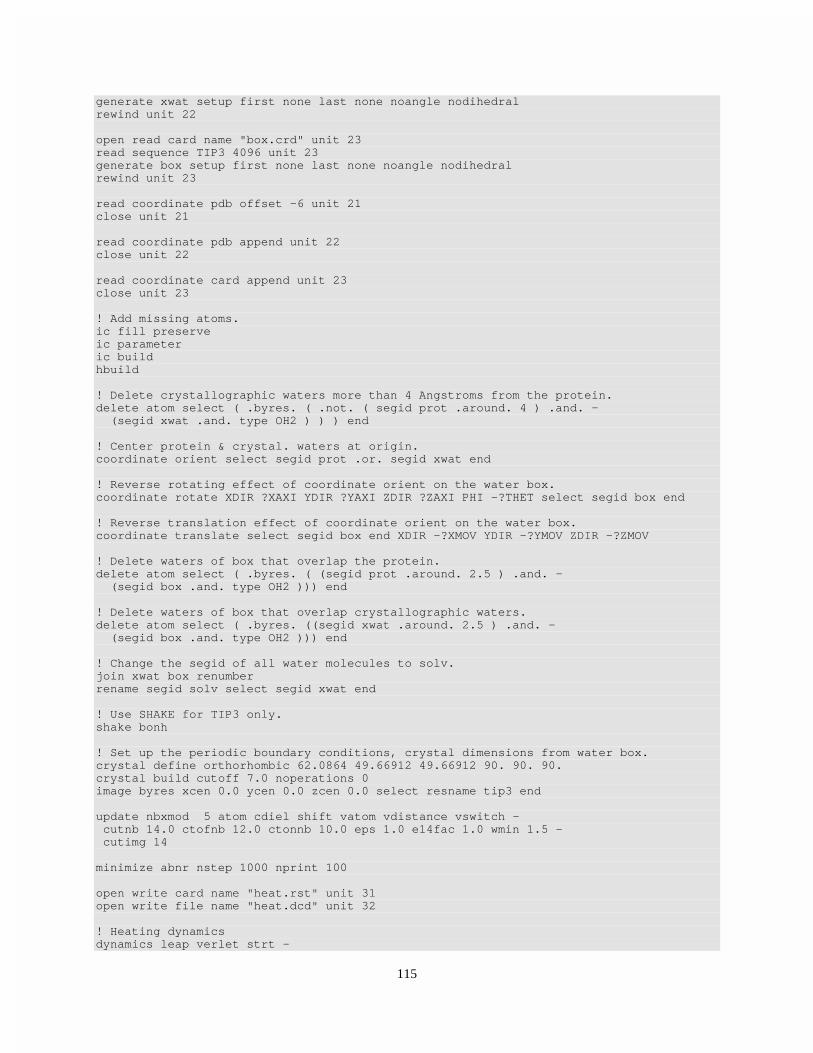
115

generate xwat setup first none last none noangle nodihedral rewind unit 22 open read card name "box.crd" unit 23 read sequence TIP3 4096 unit 23 generate box setup first none last none noangle nodihedral rewind unit 23 read coordinate pdb offset -6 unit 21 close unit 21 read coordinate pdb append unit 22 close unit 22 read coordinate card append unit 23 close unit 23 ! Add missing atoms. ic fill preserve ic parameter ic build hbuild ! Delete crystallographic waters more than 4 Angstroms from the protein. delete atom select ( .byres. ( .not. ( segid prot .around. 4 ) .and. - (segid xwat .and. type OH2 ) ) ) end ! Center protein & crystal. waters at origin. coordinate orient select segid prot .or. segid xwat end ! Reverse rotating effect of coordinate orient on the water box. coordinate rotate XDIR ?XAXI YDIR ?YAXI ZDIR ?ZAXI PHI -?THET select segid box end ! Reverse translation effect of coordinate orient on the water box. coordinate translate select segid box end XDIR -?XMOV YDIR -?YMOV ZDIR -?ZMOV ! Delete waters of box that overlap the protein. delete atom select ( .byres. ( (segid prot .around. 2.5 ) .and. - (segid box .and. type OH2 ))) end ! Delete waters of box that overlap crystallographic waters. delete atom select ( .byres. ((segid xwat .around. 2.5 ) .and. - (segid box .and. type OH2 ))) end ! Change the segid of all water molecules to solv. join xwat box renumber rename segid solv select segid xwat end ! Use SHAKE for TIP3 only. shake bonh ! Set up the periodic boundary conditions, crystal dimensions from water box. crystal define orthorhombic 62.0864 49.66912 49.66912 90. 90. 90. crystal build cutoff 7.0 noperations 0 image byres xcen 0.0 ycen 0.0 zcen 0.0 select resname tip3 end update nbxmod 5 atom cdiel shift vatom vdistance vswitch - cutnb 14.0 ctofnb 12.0 ctonnb 10.0 eps 1.0 e14fac 1.0 wmin 1.5 - cutimg 14 minimize abnr nstep 1000 nprint 100 open write card name "heat.rst" unit 31 open write file name "heat.dcd" unit 32 ! Heating dynamics dynamics leap verlet strt -

116

nstep 6000 timestep 0.001 nprint 500 nsavc 100 - nsavv 0 inbfrq -1 imgfrq 50 iprfrq 100 ihtfrq 200 - iunrea -1 iunwri 31 iuncrd 32 iunvel -1 kunit -1 - firstt 0.000000 finalt 300.0 teminc 10.0 - iasors 1 iasvel 1 iscvel 0 ichecw 0 stop

Reading Trajectories

The output of a dynamics run is contained in the trajectory file, for which the filename extension dcd is most often used. These binary format files contain multiple sets of coordinates that are usually called frames and usually, multiple frames from a trajectory are analyzed. This section shows how dcd files are read, and the following sections give examples of different calculations that use the dcd files.

Below is the relevant portion of a script for reading coordinate sets from a trajectory file. The steps of opening and reading the rtf and parameter files and the psf file appropriate to the protein are as usual and are not shown. Then, the trajectory file is opened and prepared for reading with the trajectory command (dynamc.doc). This command tells the system which unit is to be read, the first time step to be read, and the number of time steps of the original simulation to be skipped before reading another coordinate set. In this command CHARMM uses the number of time steps of the dynamics run from the beginning of a run. In general, this is much different from the number of saved coordinate sets in the dcd file. Thus, suppose in a particular run, coordinates were saved every 1000 time steps, the heating phase was 6,000 steps, the equilibration phase was 12,000 steps, and the simulation phase was 400,000 steps. To read the coordinates of the simulation phase requires a value of 19000 for the begin parameter and 1000 for the skip parameter. ! Open and read rtf, parameter, and psf files. ... ... open read file name dyn.dcd unit 51 trajectory iread 51 begin 19000 skip 1000 set i 1 label loop ! The following command reads in the next coordinate set. trajectory read ...analysis steps go here increment i if i lt 401 goto loop stop

Sometimes it is a chore to figure out the proper values for begin, particularly if a run was restarted using a rst file. The trajectory query command, open read unit 51 file name dyn.dcd trajectory query unit 15

117

will read the header information from a dcd file and output it. More useful however, is the fact that the command sets the parameters NFILE, the number of frames in the file, START, the step number of the first frame, skip, the number of steps between frames, NSTEP, the total number of steps, NDEGF, the number of degrees of freedom in the simulation, and DELTA, the step length. These can then be used in a subsequent command as illustrated below and avoids having to hard code into an analysis script the parameters needed to read coordinate sets from a dcd file. open read unit 51 file name dyn.dcd trajectory query unit 51 trajectory iread 51 begin ?start skip ?skip set i 1 label loop trajectory read ...analysis steps go here increment i if i le ?nfile goto loop stop

Calculating and Interaction Energy at Intervals During a Trajectory

The calculation of energy and of forces is central to the operation of CHARMM (energy.doc). Therefore, many options exist in the calculations of energies. For example, any of the individual contributors to energy can be singled out and calculated, for example electrostatic or bond energy, and total energy of the system or an interaction energy between parts of a system. The following example calculates the interaction energy between residues 7-20 of the dimerization domain of AraC, which constitute the N-terminal arm of the dimerization domain, and the remainder of the domain, residues 24-167. This calculation is of interest since the N-terminal arm binds to the dimerization domain over the bound arabinose and arabinose is postulated to increase the affinity of the arm for the dimerization domain. Two questions can be asked. First, whether the interaction energy between the arm and the dimerization domain in the absence of arabinose is indeed weaker than the interaction between the arm and the domain plus arabinose, and second, how well the interaction energies as calculated from the energy minimized Protein Data Bank coordinates compare to the averages of the interaction energies calculated from many frames of a molecular dynamics simulation. That is, does it appear that calculation of interaction energies from a dynamics trajectory gives more meaningful results than from a single static picture?

The following script instructs CHARMM to calculate the interaction energies between the arm and the rest of the domain and write them to an output file. This is done for each coordinate set in the output from the simulation phase of the previous example. Then, awk will be used to extract the interaction energies from the output file and average them. This example also illustrates the use of a psf file in place of reading sequence and coordinates and using the generate command to create the necessary arrays. * This file is inten.inp. * Calculates interaction energy between residues 7-20 and 24-167. * Usage, charmm <inten.inp >inten.out.

118

* ! Open and read amino acid topology and parameter files. open read card name "top_all27_prot_na.rtf" unit 20 read rtf card unit 20 close unit 20 open read card name "par_all27_prot_na.prm" unit 20 read parameter card unit 20 close unit 20 ! Open and read psf file. open read card name "fullprot.psf" unit 20 read psf card unit 20 close unit 20 ! Set up for reading coordinate sets from trajectory and writing energy data. open write card name "energy.tst" unit 52 open read file name sim.dcd unit 51 trajectory query unit 51 trajectory iread 51 begin ?start skip ?skip set i 1 ! Loop for reading coordinate sets and calculating an interaction energy. label loop trajectory read update interaction select segid prot .and. resid 7 : 20 end - select segid prot .and. resid 24 : 167 end unit 52 increment i if i le ?nfile goto loop stop

It is necessary first to open a file for writing that will contain the results of the interaction energy calculations. Then, the trajectory file is queried to determine the step and frequency parameters that must be supplied to the trajectory read command. After the query is made, this file is rewound so that coordinate frames may be read from its beginning in response to the trajectory read command. The update command updates the various lists that are used by the energy commands, and CHARMM will crash if the lists are unavailable. The interaction command selects the interactions to be calculated and directs the output to the proper file. The system being simulated here consisted of almost 9,000 atoms. To calculate the interaction energies from 400 frames requires slightly less than ten minutes.

A bit of the output in the energy.tst file is shown below. INTE ENR: Eval# ENERgy Delta-E GRMS INTE EXTERN: VDWaals ELEC HBONds ASP USER ---------- --------- --------- --------- --------- --------- INTE> 1 -149.39020 0.00000 0.57328 INTE EXTERN> -49.94151 -99.44868 0.00000 0.00000 0.00000 ---------- --------- --------- --------- --------- --------- INTE ENR: Eval# ENERgy Delta-E GRMS INTE EXTERN: VDWaals ELEC HBONds ASP USER ---------- --------- --------- --------- --------- --------- INTE> 2 -155.12775 5.73755 0.55261 INTE EXTERN> -51.45122 -103.67653 0.00000 0.00000 0.00000 ---------- --------- --------- --------- --------- ---------

119

The following awk script, avenergy.awk, for calculation of the average of the interaction energies, directs awk to maintain a sum of the energies in the s variable and to keep count of the number of energies read in the i variable. The i variable is incremented by one each time a new addition is made to the running sum of the energy. After all lines of the file have been read, the average is calculated and the results are written to the monitor. Inclusion of extra information like the number of records processed facilitates detection of errors, and is recommended. # This file is avenergy.awk # Usage, awk –f avenergy.awk <file.in { if ($1 == "INTE>") { s+=$3 i++ } } END { print "Average is " s/i, "No. records " i }

Awk can also be run directly without a script file with the following command. awk '/INTE>/ {s+=$3; i++} END {print "Average is " s/i, "No. records " i }' \ energy.tst

Note that not all single quotes are the same. Some keyboards contain more than one character that looks like a single quote, but only one will work with awk. In this case, the complete awk command became long and the Linux line continuation symbol \ was used to allow continuation of the command on a second line.

The average of the interaction energies from the 400 frames is -136 kcal/mol, which seems like an absurd value that would lead to the arm being bound to the dimerization at all times. Of course, what is relevant is the energy difference between this state and other states, and here we have not calculated the free energy or interaction energy of alternative states.

Writing out PDB Format Coordinates from a Trajectory File

Coordinates in pdb or crd format may easily be extracted from the trajectory files. The following commands perform this extraction and numbers each filename from one. They are to be placed within the trajectory read loop. The symbols @{i} direct CHARMM to substitute the value of the loop variable i in the file names and in the headers of each file. open write card name dyn@{i}.pdb unit 15 write coordinate pdb select all end unit 15 * Coordinates of protein in frame @{i} of simulation phase *

Time Series Analysis, Reading Rotamer Angles

The dihedral angles describing amino acid side chain conformations tend to be found in energy minima that are generated by steric hindrances and which differ from one another by 180 or 120 degrees. The angles are called Chi1, Chi2, etc, and the preferred conformations of a residue are called rotamers, Fig. 3.4. Glycine, of course, cannot have any Chi angles. Consider a natural protein or in a protein simulated in a molecular dynamics run. A residue lying on the surface of a protein should be relatively free to shift from one rotameric state to another while a residue on the interior of a protein will be quite constrained.

120

The correlation function of CHARMM (correl.doc) calculates a time series plus the average and rms fluctuation of whatever correl is the values of specified angles in a protein. Here we will obtain the averages and rms fluctuations of Chi1 and Chi2 of the aspartic acid residues in the dimerization domain of AraC. Time series of many quantities like bond lengths, bond angles, some energies, vector dot and cross products, temperature, and orientation can be calculated from trajectories by the correlation command without explicitly setting up a loop as was necessary in the previous example to read and calculate a quantity frame by frame. This facility is very convenient, but many of the quantities that it can calculate seem to be of primary interest to those studying and developing molecular dynamics rather than investigating protein function.

The script given below calculates the time series of Chi1 and Chi2 for Asp7 where the segment identifier is prot. As described in the documentation for the correlation function, the first command, correl, needs to be given the number of time steps that will be analyzed, the number of time series that will be calculated, and the number of atoms that will be involved. The enter commands require naming the time series that is to be calculated and then require definition of the quantity to be calculated. In this case we are using the names Chi1 and Chi2, and the atoms describing these dihedral angles are specified by segment name, residue, and atom name. After the enter commands, the trajectory command specifies which unit to read the trajectory file from, as well as which time step to begin the analysis from and how many time steps to skip between analysis operations. Finally, the write command instructs CHARMM to write out the time series of Chi1 and Chi2. The example uses the trajectory query command to extract the maximum number of frames that can be present, nfile, the step number of the first frame, start, the total number of steps in the simulation, nstep, and the skip frequency, skip. These were inserted in the correl and trajectory commands. This script runs in about half a minute. * This file is correl.inp. * Usage, charmm <correl.inp >correl.out. * Generates the chi1 and chi2 rotamer angle distributions in a trajectory. * ! Open and read amino acid topology and parameter files. open read card name "top_all27_prot_na.rtf" unit 20 read rtf card unit 20 close unit 20

NNH

CAHA

CO

CB CG

HB2 HG2

CD NE2

HE21

HE22

HB1 HG1 OE1

χ2 χ3χ1

χ1 N-CA-CB-CGχ2 CA-CB-CG-CDχ3 CB-CG-CD-OE1

Figure 3.4 Definition of Chi angles for arginine.

121

open read card name "par_all27_prot_na.prm" unit 20 read parameter card unit 20 close unit 20 ! Open and read psf file. open read card name "fullprot.psf" unit 20 read psf card unit 20 close unit 20 open read file name sim.dcd unit 51 trajectory query unit 51 open write card name rotamer.tst unit 52 correl maxtimesteps ?nfile maxseries 2 maxatoms 10 enter chi1 dihe PROT 7 N PROT 7 CA PROT 7 CB PROT 7 CG geom enter chi2 dihe PROT 7 CA PROT 7 CB PROT 7 CG PROT 7 OD1 geom trajectory firstu 51 nunit 1 begin ?start stop ?nstep skip ?skip write all card unit 52 *angles * stop

Some of CHARMM's output stream is shown below. It shows the values that had been determined by the trajectory query command and which were used by the trajectory command. As is standard with CHARMM, the title lines of the input file are reproduced in the output, allowing verification that the correct file has been analyzed. Then a summary of the calculation is provided, listing the averages and standard deviations of Chi1 and Chi2. CORREL> enter chi1 dihe PROT 7 N PROT 7 CA PROT 7 CB PROT 7 CG geom CORREL> enter chi2 dihe PROT 7 CA PROT 7 CB PROT 7 CG PROT 7 OD1 geom CORREL> trajectory firstu 51 nunit 1 begin ?start stop ?nstep skip ?skip RDCMND substituted energy or value "?START" to "13000" RDCMND substituted energy or value "?NSTEP" to "400000" RDCMND substituted energy or value "?SKIP" to "1000" The following time series will be filled: CHI1 CHI2 READING TRAJECTORY FROM UNIT 51 NUMBER OF COORDINATE SETS IN FILE: 400 NUMBER OF PREVIOUS DYNAMICS STEPS: 13000 FREQUENCY FOR SAVING COORDINATES: 1000 NUMBER OF STEPS FOR CREATION RUN: 400000 TITLE> * COORDINATES AFTER EQUILIBRATION DYNAMICS TITLE> * DATE: 11/16/ 5 18:21:25 CREATED BY USER: bob TITLE> * 388 CORD RECORDS READ FROM 1 UNITS STARTING WITH UNIT 51 RUNNING FROM STEP 13000 TO 400000 SKIPPING 1000 STEPS BETWEEN RECORDS Time step was 2.0454828E-02 AKMA time units. 1 Series "CHI1" Average = -169.235444 rms Fluctuation = 8.584620 2 Series "CHI2" Average = -83.297635 rms Fluctuation = 54.100621

The output file of the time series is shown below. Plotting or further analysis would be straightforward. The initial lines could be deleted with an editor and the data itself could be

122

directly imported into a spreadsheet program. As described in the documentation, correl can use such time series to calculate correlation functions, calculate spectral density or determine correlation times. The correl command is very powerful, and only a fraction of its capabilities has been displayed with the example given here. *ANGLES * DATE: 12/17/ 5 12:16: 9 CREATED BY USER: bob * NSER: 2 NAMES: CHI1 CHI2 TOTALS: 388 388 VECCOD: 1 1 CLASS: DIHE DIHE VELCOD: 0 0 SKIP: 1000 1000 DELTA: 0.001000 0.001000 OFFST: 1.000000 1.000000 GECOD: 1 1 VALUE: 1.000000 1.000000 1 -161.221435 -36.763926 2 -173.298686 -72.083742 3 -156.874063 -48.056556 4 -158.404703 -50.778923 ...

The dimerization domain of AraC contains five aspartic acid residues. The time series, averages, and rms fluctuations of Chi1 and Chi2 were calculated above for Asp7. The results for all the aspartic acid residues are shown in Table 3.4, where it can be seen that the rotameric states of the aspartic residues located on the surface were more free to change during the simulation than the residues located more on the interior of the protein.

Earlier versions of CHARMM running on earlier Linux versions could not run the correlation function on machines containing only 256 MB of memory. Apparently the process required more swap space than was available and the analysis would be stopped with almost no clue as to the problem. When this happens, it may be helpful to monitor the use of swap space. One way to do this is via a GNU applet that can be placed in the control bar.

Table 3.4 Rotamer Statistics of Aspartic Acid Residues in Dimerization Domain of AraC

Residue Average

Chi1

RMS Fluctuation

Chi1

Average Chi2

RMS Fluctuation

Chi2

Residue Position

Asp7 -196.2 8.5 -83.3 54.1 Surface Asp33 -167.8 6.9 46.1 13.7 Interior Asp37 -166.6 10.4 121.9 114.5 Surface Asp70 -70 7.3 -11.7 12.1 Interior Asp123 61.5 8.7 -113.4 47 Surface Asp132 -168 9.7 57.4 22 Surface

123

Problems

1. In the script mini.inp, what is accomplished by replacing minimize abnr nstep 100 nprint 20

with the following? coordinate copy comparison minimize abnr nstep 100 nprint 20 coordinate comparison rms coordinate comparison difference coordinate comparison statistics coordinate comparison distance weight coordinate copy weight scalar wmain statistics

2. Find the average distance and the maximum distance that the alpha carbon atoms of 2ARC are moved in the process of energy minimization.

3. In calculating an average distance map from a trajectory, show that, in general, averaging the coordinates and then calculating a distance map yields a different result from averaging the distance maps made from each frame of a trajectory.

4. Write an awk script that calculates the standard deviation of the energies in addition to the average of the energies using an energy output file like that described in this chapter.

5. The main limitation on increasing the size of the timestep is the high frequency of hydrogen atom oscillations. Presumably, the frequency could be reduced without affecting energy or conformational properties merely by increasing the mass of hydrogen. Where within CHARMM would this mass change be made?

6. For a moderately complex system try increasing the size of the timestep until something dramatic happens within 5,000 time steps. Then explore the functional dependence of the dramatic outcome on the size of the time step to decide whether the usual step size of 0.001 picoseconds poses any danger.

7. Measure the "evaporation" rate from a droplet of water at 1000 and 2000 degrees.

8. How many time steps of size 0.001 picoseconds are required for a sound wave to travel across a 100 Angstrom system?

Bibliography

Allen, M. and Tildesley, D. (1987). "Computer Simulation of Liquids,” Clarendon Press, Oxford. A practical guide to the writing of programs to simulate atomic and molecular liquids.

Brooks III, C., Karplus, M., and Pettitt, B. (1988). "Proteins: A Theoretical Perspective of Dynamics, Structure and Thermodynamics," John Wiley and Sons, New York. A dated but nice perspective of the field.

Essmann, U., Perera, Lalith, and Berkowitz, M. (1995). A Smooth Particle Mesh Ewald Method, J. Chem. Phys. 103, 8577-8593.

124

Leach, A. (2001). "Molecular Modeling, Principles and Applications, 2nd ed." Prentice Hall, Harlow, England. Thoroughly introduces and illustrates many techniques that are used in molecular modeling.

Rapaport, D. (1995). “The Art of Molecular Dynamics Simulation,” Cambridge University Press, Cambridge. A molecular dynamics tutorial as well as containing a large number of relevant computer programs.

Schlick, T. (2002). “Molecular Modeling and Simulation, An Interdisciplinary Guide” Series: Interdisciplinary Applied Mathematics, Vol. 21, Springer, New York. A wide-ranging introduction to modeling.

Stote, R. H., Dejaegere, A. and Karplus, M. (1997). Molecular Mechanics and Dynamics Simulations of Enzymes. Computational Approaches to Biochemical Reactivity. Netherlands, Kluwer Academic Publishers.

Related Web Sites

http://www.charmm.org The official CHARMM site. Bulletin boards, forums, on a number of CHARMM related topics are moderated by noted CHARMM experts. The place to go for help with difficult problems.

http://www.psc.edu/general/software/packages/charmm/tutorial Tutorial lectures on molecular dynamics and a number of sophisticated and general CHARMM scripts.

http://mccammon.ucsd.edu/~chem215 A very complete description of the modeling of biological macromolecules.

http://www.mdy.univie.ac.at/lehre/charmm/course1/course1.html#toc1, A CHARMM tutorial with notes and example code covering many aspects of setting up and running CHARMM simulations.

http://pekoe.chem.ukans.edu/~kuczera/Public/web/html/charmm/proc/proc.html, CHARMM Procedures for Elementary Modeling Tasks, part of an extensive web site by Krzysztof Kuczera. This shows setting up and running dynamics runs.

125

Chapter 4

Model Building Generating useful models requires the ability to create and properly position atoms. While atoms or ions may be handled individually, often it is more convenient to handle larger units consisting of entire amino acid residues or bases or groups of residues or bases, or even entire molecules. After the conceptually simple problems of creating atoms and instructing CHARMM how they are to be connected, come the more difficult problems of adjusting their conformations. Molecular mechanics assists in this operation by allowing structures to be energy minimized. Thus, structures may be constructed by specifying covalent bonds between the appropriate atoms but with impossibly long and short bond lengths. These lengths can then be corrected by energy minimizing the structure. Additional aids to the construction of models is the ability to fix some atoms in space and to pull others about while at the same time, responding properly to the presence of the rest of the structure. Examples of these types of model building operations will be presented in this chapter.

Building a Box of Water

Most molecular mechanics studies of a protein require that the protein be immersed in water. Since the structures contained in the Protein Data Bank contain only a tiny number of the water molecules surrounding a protein or DNA molecule, it is necessary computationally to create coordinate files of boxes or drops of water. In Chapter 3 a box of water molecules was used in the study of the dimerization domain of AraC. This section illustrates how such a box of water molecules may be created. The script begins by specifying the coordinates of a single molecule of water. First this is moved to the origin and then the coordinates of this molecule are assigned to a new molecule of water. The new molecule displaced in the x direction an appropriate distance to yield the correct density of water at the end of the process and then the second molecule is included in the segment identifier of the original. In the example below, the replication operation is repeated until a row of 21 water molecules has been constructed along the x axis, Fig. 4.1. This collection is then copied, row at a time, in a similar manner in the y direction to yield a square array of 441 molecules. Finally, this group is copied, square at a time, in the z direction to generate the final cubic array of 9261 water molecules.

CHARMM cannot handle unlimited numbers of atoms and residues. Version numbers before 31 are limited to 14,000 residues and 25140 atoms. In their large format, these earlier versions are limited to 32,000 residues and 120,000 atoms which is useful if larger collections of water molecules are needed. Despite these generous limits, the maximum number of residues in a segment in these earlier versions is limited to 10,000. Thus, only up to 10,000 water molecules may have the same segment identifier. Hence, the largest cubical box of water that may be constructed and used is 21 x 21 x 21 molecules and CHARMM will crash mysteriously if construction of larger boxes is attempted. When still larger boxes are required, multiple boxes, each containing less than 10,000 molecules, and each with a different segment name, must be placed beside one another or the most recent version of CHARMM must be used. * This file is waterbox.inp. * Usage, charmm <waterbox.inp >waterbox.out. * Create a box of water 21 x 21 x 21 molecules containing 9261 molecules

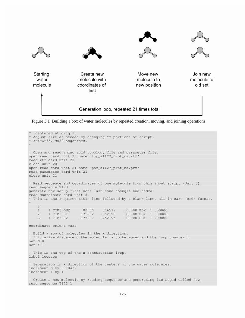
126

* centered at origin. * Adjust size as needed by changing ** portions of script. * X=Y=Z=65.19082 Angstroms. * ! Open and read amino acid topology file and parameter file. open read card unit 20 name "top_all27_prot_na.rtf" read rtf card unit 20 close unit 20 open read card unit 21 name "par_all27_prot_na.prm" read parameter card unit 21 close unit 21 ! Read sequence and coordinates of one molecule from this input script (Unit 5). read sequence TIP3 1 generate box setup first none last none noangle nodihedral read coordinate card unit 5 * This is the required title line followed by a blank line, all in card (crd) format. * 3 1 1 TIP3 OH2 .00000 .06577 .00000 BOX 1 .00000 2 1 TIP3 H1 .75902 -.52198 .00000 BOX 1 .00000 3 1 TIP3 H2 -.75907 -.52195 .00000 BOX 1 .00000 coordinate orient mass ! Build a row of molecules in the x direction. ! Initialize distance d the molecule is to be moved and the loop counter i. set d 0 set i 1 ! This is the top of the x construction loop. label looptop ! Separation in x direction of the centers of the water molecules. increment d by 3.10432 increment i by 1 ! Create a new molecule by reading sequence and generating its segid called new. read sequence TIP3 1

Starting water

molecule

Create newmolecule withcoordinates of

first

Move new molecule tonew position

Join newmolecule to

old set

Generation loop, repeated 21 times total

Figure 3.1 Building a box of water molecules by repeated creation, moving, and joining operations.

127

generate new setup first none last none noangle nodihedral ! Assign the coordinates of the first water molecule to the new molecule. coordinate duplicate select resid 1 .and. segid box end select segid new end ! Translate the new molecule a distance @d in the x direction. ! Could also use scalar x add @d select segid new end. coordinate translate XDIR @d select segid new end ! Add the new molecule to the existing molecules. join box new renumber ! Specifies **21** molecules to be built along the x axis. if i lt 21 goto looptop ! Replicate the row of molecules in the y direction. set d 0 set i 1 label loop2 increment d by 3.10432 increment i by 1 ! Create a new row of molecules, **21**. read sequence TIP3 21 generate new setup first none last none noangle nodihedral ! Assign the coordinates of the first row of old molecules to the new molecules. ! Adjust residue range to be duplicated 1:**21**. coordinate duplicate select resid 1:21 .and. segid box end select segid new end ! Translate new row of molecules a distance @d in y direction. coordinate translate YDIR @d select segid new end ! Add the new row of molecules to the existing molecules. join box new renumber ! This line specifies 21 rows molecules to be built along the y axis **21**. if i lt 21 goto loop2 ! Replicate the layer of molecules in the z direction. set d 0 set i 1 label loop3 increment d by 3.10432 increment i by 1 ! Create a new layer of molecules from the first layer. **21 x 21**. read sequence TIP3 441 generate new setup first none last none noan nodi ! Assign the coordinates of the first layer of molecules to the new molecules, **. coordinate duplicate select resid 1:441 .and. segid box end select segid new end ! translate the new layer a distance @d in the z direction. coordinate translate ZDIR @d sele segid new end ! Add the new molecule to the existing molecules join box new renumber ! This line specifies 21 layers molecules to be built along the z axis **21**. if i lt 21 goto loop3 ! Center the box at the origin.

128

coordinate orient open write card name box.pdb unit 23 write coordinates pdb select all end unit 23 * Water box 21 x 21 x 21 molecules, 65.19082 Angstroms on a side * open write card name box.crd unit 24 write coordinates sele all end card unit 24 * Water box 21 x 21 x 21 molecules, 65.19082 Angstroms on a side * stop

After reading the obligatory topology and parameter files, the script reads the sequence of one water molecule. The documentation on read and write (io.doc) shows that a sequence of TIP3 water molecules can be “read” with the command below where n is the number of molecules to be read. read sequence TIP3 n.

The appropriate scalar tables for its atoms are set up with the command generate setup (struct.doc). The noangle nodihedral options are used with TIP3 water because bond stretching and bond bending are not to occur for these atoms. Used here in the model building, there is no real need for these specifications, but they are included more as a reminder. The coordinates of the atoms are then “read” from the script. In CHARMM, in addition to the unit numbers between 10 and 80 that are available for reading and writing files, unit 5 is always the input script, and unit 6 is the output stream (usage.doc). Thus, the command open read unit 5 indicates the following portion of script is to be treated as a separate file. The coordinates will be provided in crd format, which is indicated by the command read coordinate card. read sequence TIP3 1 generate box setup first none last none noangle nodihedral read coordinate card unit 5 * This is the required title line followed by a blank line, all in card (crd) format. * 3 1 1 TIP3 OH2 .00000 .06577 .00000 BOX 1 .00000 2 1 TIP3 H1 .75902 -.52198 .00000 BOX 1 .00000 3 1 TIP3 H2 -.75907 -.52195 .00000 BOX 1 .00000

Therefore, the lines that follow duplicate what would be found in a crd format file containing the coordinates of a single molecule of TIP3 water. They include the required title lines, the number of atoms, and the coordinates as shown. The script works equally as well if instead the read coordinate indicates that a pdb file is to be read as shown below. read sequence TIP3 1 generate box setup first none last none noangle nodihedral read coordinate pdb unit 5 REMARK Now we are seeing the same information in pdb format. ATOM 1 OH2 TIP3 1 00.000 .066 00.000 1.00 0.00 BOX ATOM 1 H1 TIP3 1 .759 -.522 00.000 1.00 0.00 BOX ATOM 1 H2 TIP3 1 -.759 -.522 00.000 1.00 0.00 BOX END

129

The set command assigns values to variables or constants to regulate control flow. One of the variables is the distance molecules are to be moved, and the other is a loop counter (usage.doc). The selected molecules are moved in the x, y, and z direction by the command coordinate translate. The same effect is generated by the scalar command add (scalar.doc) and it could be used instead of the coordinate translate command. The values of variables can be set by referring directly to the variable by name, like set d 0. The value of the variable is accessed with the @ symbol, for example @d. The join and rename commands permit the joining of the atoms in two different segid's into a single segid, rename allows changing the name of a segid (struct.doc), and the coordinate orient command centers the box of water at the origin.

Constructing an Alpha Helix, Beta Sheet, Polyproline II Helix and Regular Structures

In this section a script is provided that creates a peptide with a segment identifier of pept and a sequence as defined in the script. The sequence of the peptide to be constructed is read into CHARMM (io.doc) from the script. This is given the segment identifier pept and the various associated arrays including the internal coordinate table are constructed with the generate command. In a loop that cycles once for each residue to be adjusted, the script assigns specified values to the Phi and Psi dihedrals in the internal coordinate table (intcor.doc). After this, the Cartesian coordinates are constructed. This construction requires that the position and spatial orientation of the peptide be defined by three connected atoms named in the ic seed command. The first atom named in the seed command is placed at the origin of the Cartesian coordinates. The second atom is placed on the x axis at a distance specified in the internal coordinate table as the distance between the first and second atoms. The third atom is placed in the x-y plane at a position defined by the distance from the second atom and the angle as also specified in the internal coordinate table as that defined by the three atoms.

The values to be used in the script for the Phi and Psi angles are to be included on the command line that invokes CHARMM. That is, at the command prompt one might enter the following. charmm Phi=-57 Psi=-47 <construct.inp >construct.out

As can be verified by examination of the output, CHARMM assigned the values given at the command prompt to the named variables. These values are used in the ic edit commands that adjust the values of the Phi and Psi dihedral angles. In this case the variables were those that yield an alpha helix, as can be verified by examination of the output peptide.pdb using a graphical display program like VMD.

(io.doc), (struct.doc), (intcor.doc)

It is illuminating to construct an alpha helix, a beta sheet, and the left-handed polyproline II helix. The latter structure, Fig. 4.2, is found in some structural proteins and seems to be the structure of newly synthesized polypeptide chains. Examination of this structure shows that the helix has a repeat of three, and that the side chains of the residues extend almost perpendicular to the axis of the helix.

130

* This file is construct.inp. * Usage, charmm Phi=x Psi=y <construct.inp >construct.out. * Construct a peptide of 15 residues (specified below) with phi angles set to x * and psi angles set to y. * Phi Psi * Alpha helix -57 -47 * Beta sheet -120 120 * Polyproline II Helix -75 145 * ! Open and read amino acid topology and parameter files. open read card unit 20 name "top_all27_prot_na.rtf" read rtf card unit 20 close unit 20 open read card unit 21 name "par_all27_prot_na.prm" read parameter card unit 21 close unit 21 ! Read sequence of 15 residue peptide from this input script (Unit 5). read sequence card * This is the mandatory title * 15 ALA ALA ALA ALA ALA ARG ARG ARG ARG ARG GLY GLY GLY GLY GLY ! Setup arrays for the peptide, fill ic table from residue topology file. generate pept setup ! Complete ic table, if necessary using values from parameter file. ic parameter ! Each cycle through loop changes phi of a residue and psi of the next residue. ! Note that first residue has only a psi dihedral and last residue only a phi. set resno 1

Figure 4.1 Arg-15 in a polyproline-II helix seen largely in side view and largely in end view.

131

set nextres 2 label loop ! Adjust the dihedrals phi of residue numbered nextres and psi of residue ! numbered resno to the passed values Phi and Psi. ic edit dihedral @resno C @nextres N @nextres CA @nextres C @Phi dihedral @resno N @resno CA @resno C @nextres N @Psi end increment resno increment nextres if resno lt 15 goto loop ! Having set internal coordinates, now build Cartesian coordinates. ic seed 1 N 1 CA 1 C ic build ! Write out Cartesian coordinates of the peptide. open write card name peptide.pdb unit 30 write coordinates pdb select all end unit 30 * Peptide with all phi set to @Phi and all psi set to @Psi * stop

Fixing, Restraining, and Pulling Atoms

Atoms may be fixed in place with the command constrain fix select <atom> end

and they may be restrained to the vicinity of a point with an attractive potential that increases in magnitude the further the atom is from the point (cons.doc). Both the magnitude of the attractive potential and the rate at which the potential increases with increasing distance may be assigned. Fixing of course holds an atom immobile whereas restraining allows an atom to move during energy minimization or in a dynamics simulation but in accordance the various forces acting on the atom plus the force imposed by the restraining potential.

In modeling one may want to build a peptide of a specific sequence bend it, and connect it to a protein. Generation of a peptide of any sequence and length is straightforward, as illustrated in the previous section. Here we show how parts of a peptide or protein can be pushed or pulled about so as to bend a peptide or distort a protein. In a later section a script will be developed that connects two different proteins. A peptide as a whole can be moved about with respect to a protein with the coordinate translate command by selecting only the atoms of the peptide. This allows rigidly moving the entire peptide so as to place one end at a desired position. Then, this end of the peptide can be immobilized by fixing an atom or residue in place while an atom from the other end is gently pulled during an energy minimization by the assignment of an attractive potential centered at the desired endpoint of the atom’s movement. After this, the center of the attractive potential can be moved again and the system can be energy minimized again. By allowing the peptide or protein to move in response to the artificial potential that is pulling it plus the real potentials generated by the atoms of the rest of the system, the peptide assumes conformations and interacts with the rest of the system in ways that are close to what must occur naturally. This seems better than blindly forcing the peptide into a fully predetermined structure.

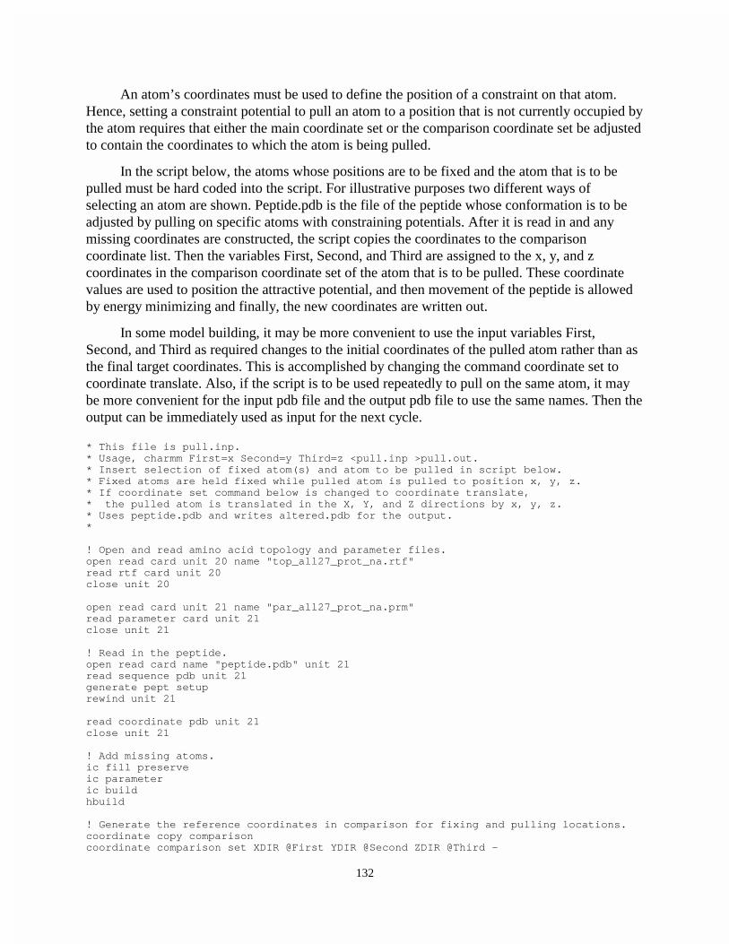
132

An atom’s coordinates must be used to define the position of a constraint on that atom. Hence, setting a constraint potential to pull an atom to a position that is not currently occupied by the atom requires that either the main coordinate set or the comparison coordinate set be adjusted to contain the coordinates to which the atom is being pulled.

In the script below, the atoms whose positions are to be fixed and the atom that is to be pulled must be hard coded into the script. For illustrative purposes two different ways of selecting an atom are shown. Peptide.pdb is the file of the peptide whose conformation is to be adjusted by pulling on specific atoms with constraining potentials. After it is read in and any missing coordinates are constructed, the script copies the coordinates to the comparison coordinate list. Then the variables First, Second, and Third are assigned to the x, y, and z coordinates in the comparison coordinate set of the atom that is to be pulled. These coordinate values are used to position the attractive potential, and then movement of the peptide is allowed by energy minimizing and finally, the new coordinates are written out.

In some model building, it may be more convenient to use the input variables First, Second, and Third as required changes to the initial coordinates of the pulled atom rather than as the final target coordinates. This is accomplished by changing the command coordinate set to coordinate translate. Also, if the script is to be used repeatedly to pull on the same atom, it may be more convenient for the input pdb file and the output pdb file to use the same names. Then the output can be immediately used as input for the next cycle. * This file is pull.inp. * Usage, charmm First=x Second=y Third=z <pull.inp >pull.out. * Insert selection of fixed atom(s) and atom to be pulled in script below. * Fixed atoms are held fixed while pulled atom is pulled to position x, y, z. * If coordinate set command below is changed to coordinate translate, * the pulled atom is translated in the X, Y, and Z directions by x, y, z. * Uses peptide.pdb and writes altered.pdb for the output. * ! Open and read amino acid topology and parameter files. open read card unit 20 name "top_all27_prot_na.rtf" read rtf card unit 20 close unit 20 open read card unit 21 name "par_all27_prot_na.prm" read parameter card unit 21 close unit 21 ! Read in the peptide. open read card name "peptide.pdb" unit 21 read sequence pdb unit 21 generate pept setup rewind unit 21 read coordinate pdb unit 21 close unit 21 ! Add missing atoms. ic fill preserve ic parameter ic build hbuild ! Generate the reference coordinates in comparison for fixing and pulling locations. coordinate copy comparison coordinate comparison set XDIR @First YDIR @Second ZDIR @Third –

133

select atom pept 15 CA end ! Assign the constraints. constrain fix select segid pept .and.(resid 1 .or. resid 5) .and. type CA end constrain harmonic comparison expo 2 force 5 - select segid pept .and. resid 15 .and. type CA end ! Perform the pulling by energy minimizing. minimize abnr nstep 1000 nprint 100 ! Write out Cartesian coordinates of the peptide. open write card name peptide.pdb unit 30 write coordinates pdb select all end unit 30 * Peptide after pulling * stop

Changing, or Mutating Residues

Often one has the coordinates of a protein and wishes to calculate something about the structure or energetics of a variant of the protein where the identity of an amino acid is changed. Two issues must be addressed in computationally mutating a protein. The first is the altering the residue, that is, changing the name of the residue and its structure as understood by CHARMM. The second is adjusting the conformation or rotameric state of the side chain to that appropriate for the protein. This second issue may sometimes be addressed by assigning the different rotameric states and energy minimizing to find the one of lowest free energy. Programs also exist that predict rotameric states of residues (Canutescu et al. 2003). This section addresses the process of changing the residue name and the side chain of the mutated residue, and the next section addresses the problem of changing the conformation of a new side chain.

The script for mutating a protein is passed a segid that will be assigned to the mutated protein, the residue number for the mutation resno, and the identity of the new amino acid, new. The steps that are required to change a residue of a protein are not complicated, Fig. 4.3. The sequence and coordinates of the protein are read in and the psf is generated. After this the side chain of the desired residue is deleted, the name of the residue name is changed, and then the side chain of the renamed residue is rebuilt using the internal coordinates in the residue topology table. If proline is involved in the process, intermediates in the mutation process may possess nonintegral electric charge, in which case CHARMM issues a warning and normally quits. This undesirable behavior can be prevented simply by changing the bomb level to –1 with the command bomb –1. After deleting the side chain atoms and renaming the residue, the protein's coordinates are written to a temporary file. CHARMM is thus cleared of all memory of the protein, and the temporary file is read back into CHARMM. Because it is the new sequence that is read in, the new internal arrays are constructed for the new sequence, that is, the mutated sequence. The internal coordinate tables are then used to provide coordinates for the side chain atoms of the mutated residue, and finally, the coordinates of the mutated protein are written to a file. One could code the desired amino acid changes into a script, but for elegance a general script can be constructed that will allow passing the residue and alteration to CHARMM in the command line. * This file is mutate.inp. * Usage, charmm segid=wxyz resno=n new=abc <mutate.inp >mutate.out * where wxyz is the segid of the protein, n is the resnumber, and abc is * the three letter abbreviation of the new residue at position n.

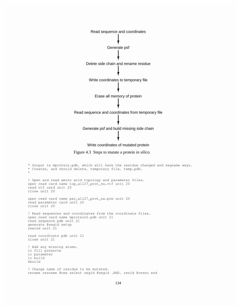
134

* Output is mprotein.pdb, which will have the residue changed and segname wxyz. * Creates, and should delete, temporary file, temp.pdb. * ! Open and read amino acid topology and parameter files. open read card name top_all27_prot_na.rtf unit 20 read rtf card unit 20 close unit 20 open read card name par_all27_prot_na.prm unit 20 read parameter card unit 20 close unit 20 ! Read sequences and coordinates from the coordinate files. open read card name mprotein2.pdb unit 21 read sequence pdb unit 21 generate @segid setup rewind unit 21 read coordinate pdb unit 21 close unit 21 ! Add any missing atoms. ic fill preserve ic parameter ic build hbuild ! Change name of residue to be mutated. rename resname @new select segid @segid .AND. resid @resno end

Read sequence and coordinates

Generate psf

Delete side chain and rename residue

Write coordinates to temporary file

Erase all memory of protein

Read sequence and coordinates from temporary file

Generate psf and build missing side chain

Write coordinates of mutated protein

Figure 4.3 Steps to mutate a protein in silico.

135

! So CHARMM won't complain about nonintegral net charges when proline is involved. bomb -1 ! Delete side chain atoms. delete atom select segid @segid .and. resid @resno .and. - .not. (type n .or. type ca .or. type c .or. type o .or. type ha .or. type hn) end ! Store the mutated protein that lacks the mutated side chain open write card name temp.pdb unit 14 write coordinates pdb select all end unit 14 *Temporary * close unit 14 ! Remove all memory from CHARMM of the protein delete atom select all end ! Read in the protein (missing side chain atoms on the residue ! to be mutated and with this residue given the new name). open read card name temp.pdb unit 14 read sequence pdb unit 14 generate @segid setup rewind unit 14 read coordinate pdb unit 14 close unit 14 ! Adds the side chain atoms to mutated residue. ic fill preserve ic parameter ic build hbuild open write card name mprotein3.pdb unit 14 write coordinates pdb select all end unit 14 *Coordinates of mutated protein. Residue @resno changed to @new * ! Delete the temporary coordinates with this system command system "rm temp.pdb" stop

Adjusting Rotameric State

Modeling of proteins can require adjustment of side chain conformations. These conformations are specified by dihedral angles Chi1, Chi2, etc. of atoms along the side chain as was mentioned in the previous chapter and illustrated in Fig. 3.4. Glycine, of course, cannot have any Chi angles. As discussed in Chapter 2, steric hindrance between atoms of the side chain and sometimes the main chain generate energy minima such that the Chi angles in amino acids tend to be found in energy minima that differ from one another by 120 or by 180 degrees. The different specific conformations of a side chain are called rotamers. One question that arises in computing properties of a mutated protein is deciding which of the rotameric states of that residue should be used. Often good guesses can be made by choosing the rotameric state that is found most often in proteins, or the rotameric state that minimizes clashes with adjacent atoms. This section does not further address the issue of choosing rotameric states, but merely indicates how the side chain of a residue may be adjusted by CHARMM. The alteration may be performed using internal coordinates or Cartesian coordinates. .

136

The script given below reads in pdb coordinates of a protein, which, of course, must first have been sanitized by fixpdb.awk. The rotamer script adjusts the Chi angle that is defined by the four atoms specified on the command line used to invoke CHARMM. Reference to the rtf shows that if Chi1 is being set, the four atoms that define Chi1 are N, CA, CB, and CG. After setting the value of the dihedral angle in the internal coordinates, the regular coordinates of the rotated side chain must be reconstructed with the ic build command. Before this can be done however, the coordinates of these side chain atoms must be initialized so the their new values will be recalculated by the ic build command. Otherwise these values would remain unaltered... * This file is rotadjust.inp. * Usage, charmm resid=int atom1=atomname atom2=atomname atom3=atomname * atom4=atomname chi=value <rotadjust.inp >rotadjust.out, * where resid is the residue number being modified and * atom1 through atom4 give the names of the atoms defining the dihedral angle. * Produces an output pdb with dihedral set to value of chi. * ! Open and read amino acid topology and parameter files. open read card name "top_all27_prot_na.rtf" unit 20 read rtf card unit 20 close unit 20 open read card name "par_all27_prot_na.prm" unit 20 read parameter card unit 20 close unit 20 ! Read sequences and coordinates from the coordinate files. open read card name "protein.pdb" unit 21 read sequence pdb unit 21 generate prot setup rewind unit 21 read coordinate pdb offset -6 unit 21 close unit 21 ! Add missing atoms. ic fill preserve ic parameter ic build hbuild ! Adjust dihedral with ic edit using the passed variables. ic edit dihedral prot @resid @atom1 prot @resid @atom2 prot @resid @atom3 – prot @resid @atom4 @chi end ! Erase coordinates of the side chain in coordinate array. coordinate initialize select segid prot .and. resid @resid .and. - .not. (type n .or. type ca .or. type c .or. type o .or. type ha .or. type hn) end ! Rebuild the rotated side chain in coordinate space ic build ! Write output open write card unit 17 name out.pdb write coordinate pdb select all end unit 17 *Chi of resid @resid defined by @atom1 @atom2 @atom3 @atom4 set to @chi * stop

137

Use of Patches for Special Structures

Proteins often contain more substructures than the standard twenty amino acids. For example, the amino terminal and carboxyl terminal amino acids possess different structures than the internal residues. These altered structures are generated by sets of instructions known as patches. Earlier chapters implicitly used patches in response to the generate command. By default, without explicit naming of the patches to be used for modifying the N- and C-termini of proteins, the generate command uses the patches NTER and CTER which are mentioned near the beginning of the residue topology file (struct.doc). The patches themselves are located further into the file. The file should be examined to gain an idea of patches they work as well as to see what other patches exist. One finds that the NTER patch is not suitable for generation of the N-terminus of proteins that begin either with glycine or proline, and instead, the patches needed to generate the correct N-terminal structures of these two amino acids are GLYP and PROP. Hence, the correct generate command for a protein beginning with glycine would be generate prot first GLYP setup

Another example the use of a patch would be specifying that the N-terminus of a protein be acetylated. This might be a sensible way to remove the positive charge from the N-terminus of a protein. By looking through the rtf file, it can be seen that the patch for acetylating the N-terminus is ace. This patch is applied during the generation of the coordinate and internal coordinate tables. Thus, the command for doing this is. generate prot first ace setup

instead of generate prot setup.

Other patches are applied after generation of the tables. For example, a protein may contain two disulfide bonds, one between residues 7 and 40 and the other between residues 20 and 50. After reading in the protein's sequence, the following commands are needed to generate the psf and internal coordinate table and to modify the psf table so as to indicate the presence of the two disulfide bonds. generate prot setup patch disu prot 7 prot 40 patch disu prot 20 prot 50

The patch command forces adjustment of the psf and the various internal tables of CHARMM. If the patch adds atoms to the structure the mention of the new atoms in the patch tells CHARMM to create slots for them in the various arrays. Similarly, the patch must list all the new bond, angle, and dihedral energy terms that involve the new atoms so that these terms my be added to the psf. Issuing a patch command does not generate values for the Cartesian coordinates of the new atoms. These may be read in from a coordinate file, or, if the patch contains the internal coordinate information for the new atoms, the values of the missing coordinates can be generated with ic parameter and ic build commands following the patch command. Missing

138

hydrogen atoms can be added with the hbuild command. Patches can be added to the residue topology file, or the can be read in separately after the main rtf file, (io.doc).

Constructing a Quick and Dirty Patch for the GFP Chromophore

A patch (struct.doc) is very similar to one of the residue entries in the rtf. Instead, however, of specifying the relevant structure de novo, only the changes that are needed to go from a structure contained in the rtf to the desired structure are specified. The first line of a patch is the identifier PRES for patch residue, the name of up to four letters identifying the patch, and the sum of the charges of the following lines that specify atoms. Then, the patch contains a list of atoms. These are atoms that are added, or are atoms whose atom types or charges are to be changed, and any atoms that are to be deleted. A patch that is applied after the generate command cannot use the autogenerate angles and autogenerate dihedrals command. Therefore, such a patch must explicitly list every angle, dihedral, and improper that includes any of the new atoms. Finally, the patch may contain a list of internal coordinates that would be used in conjunction with ic build for proper placement of any new atoms. Patches lacking internal coordinate specifications will work if the coordinates of all the nonhydrogen atoms are contained in the input coordinate file and do not need to be generated using internal coordinate values and the ic build command.

Suppose the green fluorescent protein is to be included in a simulation but that the details of the vibrations of the protein's fluorophore are not important. The GFP fluorophore is derived from three consecutive amino acids. In one form of the protein these are serine, tyrosine, and glycine that are cyclized by an oxidation that joins the serine and glycine, Fig. 4.4. The Protein Data Bank structures of GFP contain the locations of all the heavy atoms, and the hbuild features of CHARMM can position the missing hydrogen atoms. Thus, the structure of the GFP protein containing the fluorophore can be approximated merely by instructing CHARMM as to which atoms of the serine, tyrosine, and glycine are to be deleted, where the new bond is to be formed

HN

N CA

HA

CB

OG HG1

HB1HB1

C

N

O

HN

CA

HA

CB HB2HB1

C

O

N

HN

CA C

HA1

HA2 O

OHSer

Tyr

Gly

Atom to be deleted

Atom to be changed

HN C

H

C

OH

HH

C

N

C

CN

CHH

C

O

CH

OH

O

New bond

(-)

(1)

(+)

Figure 4.4 Modificatioins to Ser Tyr Gly that are needed to generate the GFP fluorophore.

139

and what new angle and dihedral energy terms must be added. The figure shows the serine, tyrosine, and glycine, the atoms that are to be deleted, the atoms whose types or partial charges need to be changed, and the final fluorophore structure. The statement required to effect the changes defined in the patch would be similar to the following where gfp refers to the name of the patch, prot is the segment identifier of the protein, and residue 66 is the tryosine of the ultimate fluorophore. This command would follow the generate setup command for the protein itself. patch gfp prot 66

A plus sign immediately preceding the atom identifier refers to the next residue, which is Gly, and a minus sign refers to the previous residue, which is Ser. By reference to the list of atom types at the beginning of the rtf table and guessing partial charges of the relevant atoms, the lines can be written to retype the four atoms, delete the five atoms, and specify the new bond that links serine and glycine. In order that the psf contain all the angle and dihedral energy terms, all the new angles and new dihedrals that involve the new bond, Fig. 4.4 must be listed. All these terms must be included because the energy terms in the parameter file have been chosen with the convention that every dihedral present will be listed. This means every possible way of listing a dihedral must be included. This seemingly strange definition is a result of the fact that autogenerate produces lists of angles and dihedrals that list all possible definitions, and the same parameters must be used both for entries in the psf that result from the autogenerate command as well as from entries in patches like this one, in which all the angles and dihedrals are listed by hand. PRES GFP -0.07 ! Usage patch gfp segname resid. ! Makeshift patch for cyclizing Ser-Tyr-Gly to form gfp fluorophore. ! Charges guessed, bonds and atom types wrong, but topology is correct. ! Cannot be used to place heavy atoms missing in input coordinate data. ATOM 1N N -0.37 ATOM 1+N N -0.35 ATOM 1+C C +0.70 ATOM 1CA CT1 -0.05 DELETE ATOM 1+HN ! That is, delete the HN atom from the next residue, 67. DELETE ATOM 1-O DELETE ATOM 1HB2 DELETE ATOM 1HN DELETE ATOM 1HA BOND 1-C 1+N angle -CA -C +N 1N -C +N angle -C +N +CA -C +N 1C dihedral -CB -CA -C +N -N -CA -C +N dihedral -HA -CA -C +N -CA -C +N 1C dihedral -CA -C +N +CA -CA -C +N +HN dihedral -C +N 1C 1O -C +N 1C 1CA dihedral -C +N +CA +HA1 -C +N +CA +HA2 dihedral -C +N +CA +C

This patch ignores the definition of groups of atoms with integral charge. This omission will generate no difficulties as long as the default is used in which electrostatic interactions are calculated on an atom basis rather than a group basis.

140

Writing a Residue Topology File Ligand Entry for Arabinose

Entries for many small molecules can be found in the topology files that accompany CHARMM. Nonetheless, sometimes the analysis of a protein will require handling a small molecule whose structure is not already present in the rtf. Dealing with such a new ligand seems like a chicken and egg problem. CHARMM can not read coordinate files containing the new ligand without a corresponding RESI residue topology file entry, but it may need the coordinates to generate a complete topology file entry. The solution is to write enough of a residue topology file that CHARMM can read in the coordinates and then to use them to complete the entry.

Here the process of generating a complete rtf file entry for L-arabinose is outlined. The necessary steps seem complicated but are not. A good starting point is the ribose portion of the rtf entry for any one of the nucleotides in the topology file top_all27_prot_na.rtf. This will provide a pattern for the atom types and the partial charges that are appropriate for use with the topology file and par_all27_prot_na.prm parameter file. Helpful information can also be extracted from the rtf file for glucose which is shown below and which is found in top_all22_sugar.inp. An input pdb coordinate file containing the coordinates of all the carbon and oxygen atoms of arabinose is also needed. * Topology file for alpha-D-glucopyranose monomer. * 10/13/94 , Guyan Liang and John Brady * 22 1 MASS 4 HT 1.00800 H ! TIP3P water hydrogen MASS 56 OT 15.99940 O ! TIP3P water oxygen MASS 73 HAS 1.00800 H ! sugar aliphatic hydrogen MASS 74 HOS 1.00800 H ! sugar hydroxyl hydrogen MASS 75 CTS 12.01100 C ! sugar aliphatic carbon MASS 78 CBS 12.01100 C ! C1 in beta sugars MASS 76 OHS 15.99940 O ! sugar hydroxy oxygen MASS 77 OES 15.99940 O ! sugar ring oxygen AUTOGENERATE angles dihedrals ! DEFAults for patching FIRSt and LAST residues DEFA FIRST NONE LAST NONE RESI AGLC 0.000 ! 4C1 alpha-D-glucopyranose monomer ! GROU ! ATOM C1 CTS 0.200 ! O6-HO6 ATOM H1 HAS 0.090 ! | ATOM O1 OHS -0.660 ! H61-C6-H62 ATOM HO1 HOS 0.430 ! | ATOM C5 CTS 0.250 ! C5---O5 ATOM H5 HAS 0.090 ! H4 /| \ O1-HO1 ATOM O5 OES -0.400 ! \ / H5 HO2 \ / GROU ! C4 | C1 ATOM C2 CTS 0.140 ! / \ H3 O2 / \ ATOM H2 HAS 0.090 ! HO4-O4 \| | / H1 ATOM O2 OHS -0.660 ! C3---C2 ATOM HO2 HOS 0.430 ! | | GROU ! HO3-O3 H2 ATOM C3 CTS 0.140 ! ATOM H3 HAS 0.090 ! ATOM O3 OHS -0.660 ! ATOM HO3 HOS 0.430 ! GROU ATOM C4 CTS 0.140 ATOM H4 HAS 0.090 ATOM O4 OHS -0.660

141

ATOM HO4 HOS 0.430 GROU ATOM C6 CTS 0.050 ATOM H61 HAS 0.090 ATOM H62 HAS 0.090 ATOM O6 OHS -0.660 ATOM HO6 HOS 0.430 BOND C1 O1 C1 H1 O1 HO1 C1 O5 C1 C2 BOND C2 H2 C2 O2 O2 HO2 C2 C3 C3 H3 BOND C3 O3 O3 HO3 C3 C4 C4 H4 C4 O4 BOND O4 HO4 C4 C5 C5 H5 C5 C6 C6 H61 BOND C6 H62 C6 O6 O6 HO6 C5 O5 DONO BLNK HO1 DONO BLNK HO2 DONO BLNK HO3 DONO BLNK HO4 DONO BLNK HO6 ACCE O1 ACCE O2 ACCE O3 ACCE O4 ACCE O5 ACCE O6 ! I J K L R(IK) T(IKJ) PHI T(JKL) R(KL) IC O1 C2 *C1 H1 1.3889 109.35 -122.69 108.98 1.0950 IC O1 O5 *C1 C2 1.3889 111.55 -121.57 110.06 1.5340 IC O2 C3 *C2 H2 1.4154 112.27 -118.21 108.23 1.0919 IC O2 C1 *C2 C3 1.4154 110.87 -125.56 111.08 1.5253 IC O3 C4 *C3 H3 1.4157 110.61 120.65 108.81 1.1068 IC O3 C2 *C3 C4 1.4157 108.09 120.77 109.86 1.5177 IC O4 C5 *C4 H4 1.4252 110.90 -120.61 108.35 1.1024 IC O4 C3 *C4 C5 1.4252 108.31 -122.08 111.17 1.5287 IC C6 O5 *C5 H5 1.5099 108.10 118.69 109.65 1.1042 IC C6 C4 *C5 O5 1.5099 111.57 119.10 108.69 1.4274 IC O6 H62 *C6 H61 1.4132 110.47 -120.32 107.85 1.0945 IC O6 C5 *C6 H62 1.4132 110.45 -121.53 108.99 1.0959 IC O5 C1 C2 C3 1.4254 110.06 54.09 111.08 1.5253 IC C1 C2 C3 C4 1.5340 111.08 -51.23 109.86 1.5177 IC C2 C3 C4 C5 1.5253 109.86 53.25 111.17 1.5288 IC C3 C4 C5 O5 1.5177 111.17 -57.46 108.69 1.4274 IC C4 C5 O5 C1 1.5288 108.69 62.25 113.77 1.4254 IC C5 O5 C1 C2 1.4274 113.77 -60.97 110.06 1.5340 IC C4 C5 C6 O6 1.5287 111.57 -170.28 110.45 1.4132 IC O5 C1 O1 HO1 1.4254 111.55 74.87 107.83 0.9684 IC C1 C2 O2 HO2 1.5340 110.87 -100.51 112.13 0.9638 IC C2 C3 O3 HO3 1.5253 108.09 -165.88 112.08 0.9730 IC C3 C4 O4 HO4 1.5177 108.31 134.18 106.97 0.9713 IC C5 C6 O6 HO6 1.5099 110.44 -143.88 107.72 0.9641 PATC FIRS NONE LAST NONE PRES BETA 0.200 ! patch to make the C1 group equatorial (beta) ! use in generate statement ATOM C1 CBS 0.200 IC O1 C2 *C1 H1 1.3890 105.75 114.54 108.17 1.0950 IC O1 O5 *C1 C2 1.3890 111.55 117.06 110.06 1.5340 END

We will add the new residue entry for arabinose to the existing rtf file. Because the existing topology file contains the autogenerate angles commands there is no need to list all the angles and dihedrals in the topology file entry for arabinose since these energy terms will be created automatically. The topology file also contains the instruction to apply the NTER and CTER structure modification patches to the first and last residues by default. To prevent this automatic and, in this case, inappropriate application of these patches when the sequence file is read by

142

CHARMM, the generate command in a script that will be reading in arabinose will need to override the automatic application. To generate the segment identifier LIGA for a residue of arabinose whose “sequence” has just been read is done as follows. generate LIGA first none last none

In the topology file the residue name for arabinose will be ARA, and its charge will be 0.000 . To write more of the file, the structure can be drawn on paper, taking care to name the atoms as they are named in the input coordinate pdb file. The nomenclature may be explained in the pdb source file, or if not, it can be determined by examination of the file in conjunction with observing the molecule with a molecular display program like VMD, Fig. 4.5. The atom names can be assigned to CHARMM atom types and partial charges can be guess by comparison to the topology file entries for glucose and ribose. Below this has been done. ! RTF for L-arabinose, based on ribose and glucose RESI ARA 0.000 GROUP ATOM C1 CN7B 0.240 ATOM O1 ON5 -0.660 ! H51 ATOM HO1 HN5 0.430 ! | ATOM H1 HN7 0.090 ! C5---O5 ATOM C5 CN8 0.240 ! H4 /| \ O1-HO1 ATOM O5 ON6B -0.520 ! \ / H52 HO2\ / ATOM H51 HN7 0.090 ! C4 | C1 ATOM H52 HN7 0.090 ! / \ H3 O2/ \ ! HO4-O4 \| |/ H1 GROUP ! C3---C2 ATOM C2 CN7B 0.140 ! | | ATOM O2 ON5 -0.660 ! HO3-O3 H2 ATOM HO2 HN5 0.430 ATOM H2 HN7 0.090 GROUP ATOM C3 CN7B 0.140 ATOM O3 ON5 -0.660 ATOM HO3 HN7 0.430 ATOM H3 HN7 0.090 GROUP ATOM C4 CN7B 0.140 ATOM O4 ON5 –0.660 ATOM HO4 HN5 0.430

O5

C1O1

C2

O2C3O3

C4

O4

C5

Figure 4.5 Atom names in L-arabinose as viewed in the graphical display program VMD.

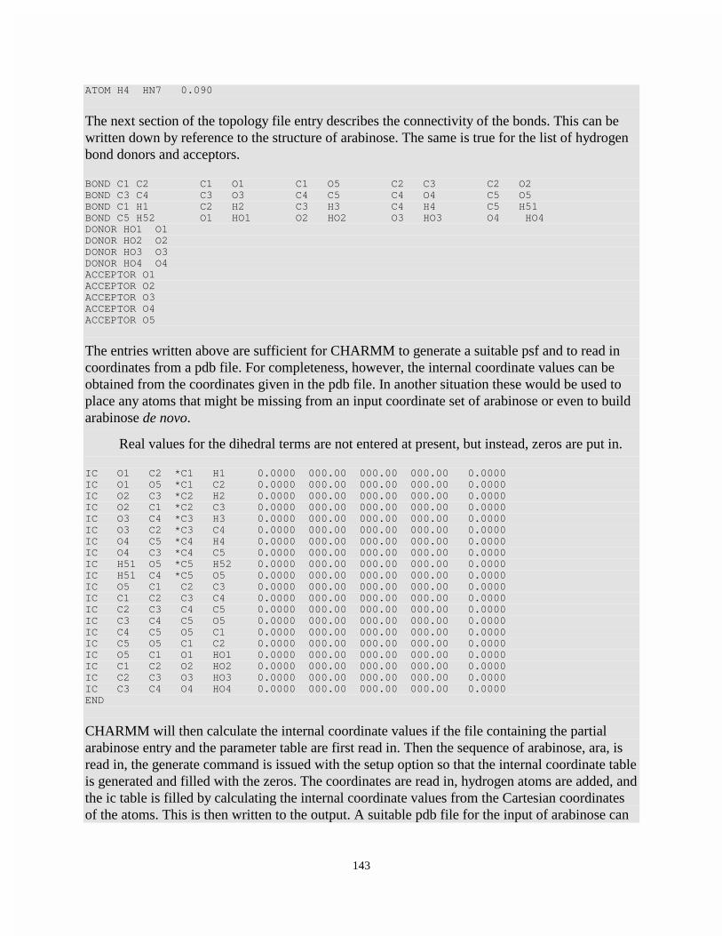
143

ATOM H4 HN7 0.090

The next section of the topology file entry describes the connectivity of the bonds. This can be written down by reference to the structure of arabinose. The same is true for the list of hydrogen bond donors and acceptors. BOND C1 C2 C1 O1 C1 O5 C2 C3 C2 O2 BOND C3 C4 C3 O3 C4 C5 C4 O4 C5 O5 BOND C1 H1 C2 H2 C3 H3 C4 H4 C5 H51 BOND C5 H52 O1 HO1 O2 HO2 O3 HO3 O4 HO4 DONOR HO1 O1 DONOR HO2 O2 DONOR HO3 O3 DONOR HO4 O4 ACCEPTOR O1 ACCEPTOR O2 ACCEPTOR O3 ACCEPTOR O4 ACCEPTOR O5

The entries written above are sufficient for CHARMM to generate a suitable psf and to read in coordinates from a pdb file. For completeness, however, the internal coordinate values can be obtained from the coordinates given in the pdb file. In another situation these would be used to place any atoms that might be missing from an input coordinate set of arabinose or even to build arabinose de novo.

Real values for the dihedral terms are not entered at present, but instead, zeros are put in. IC O1 C2 *C1 H1 0.0000 000.00 000.00 000.00 0.0000 IC O1 O5 *C1 C2 0.0000 000.00 000.00 000.00 0.0000 IC O2 C3 *C2 H2 0.0000 000.00 000.00 000.00 0.0000 IC O2 C1 *C2 C3 0.0000 000.00 000.00 000.00 0.0000 IC O3 C4 *C3 H3 0.0000 000.00 000.00 000.00 0.0000 IC O3 C2 *C3 C4 0.0000 000.00 000.00 000.00 0.0000 IC O4 C5 *C4 H4 0.0000 000.00 000.00 000.00 0.0000 IC O4 C3 *C4 C5 0.0000 000.00 000.00 000.00 0.0000 IC H51 O5 *C5 H52 0.0000 000.00 000.00 000.00 0.0000 IC H51 C4 *C5 O5 0.0000 000.00 000.00 000.00 0.0000 IC O5 C1 C2 C3 0.0000 000.00 000.00 000.00 0.0000 IC C1 C2 C3 C4 0.0000 000.00 000.00 000.00 0.0000 IC C2 C3 C4 C5 0.0000 000.00 000.00 000.00 0.0000 IC C3 C4 C5 O5 0.0000 000.00 000.00 000.00 0.0000 IC C4 C5 O5 C1 0.0000 000.00 000.00 000.00 0.0000 IC C5 O5 C1 C2 0.0000 000.00 000.00 000.00 0.0000 IC O5 C1 O1 HO1 0.0000 000.00 000.00 000.00 0.0000 IC C1 C2 O2 HO2 0.0000 000.00 000.00 000.00 0.0000 IC C2 C3 O3 HO3 0.0000 000.00 000.00 000.00 0.0000 IC C3 C4 O4 HO4 0.0000 000.00 000.00 000.00 0.0000 END

CHARMM will then calculate the internal coordinate values if the file containing the partial arabinose entry and the parameter table are first read in. Then the sequence of arabinose, ara, is read in, the generate command is issued with the setup option so that the internal coordinate table is generated and filled with the zeros. The coordinates are read in, hydrogen atoms are added, and the ic table is filled by calculating the internal coordinate values from the Cartesian coordinates of the atoms. This is then written to the output. A suitable pdb file for the input of arabinose can

144

be extracted from the 2ARC.PDB file and then processing with fixpdb.awk using a segment identifier of LIGA. All of this is shown in the script below. * This file is buildrtf.inp. * Usage, charmm <buildrtf.inp >buildrtf.out. * For generating values for ic coordinates of arabinose rtf. * Input files, top_all27_prot_na.rtf, par_all27_prot_na.prm, ara.pdb. * ! Open and read topology and parameter files. open read card unit 20 name "top_all27_prot_na.rtf" read rtf card unit 20 close unit 20 open read card unit 20 name "par_all27_prot_na.prm" read parameter card unit 20 close unit 20 ! Open and read sequence of arabinose. open read unit 14 card name "ara.pdb" read sequence pdb unit 14 generate liga setup first none last none rewind unit 14 read coordinate pdb unit 14 close unit 14 ! Add hydrogen atoms to arabinose hbuild ! Transfer coordinates to internal coordinates ic fill !Output the internal and Cartesian coordinates print ic print coordinate stop

The script above uses the incomplete rtf to enable CHARMM to read in the coordinates of the heavy atoms of arabinose, add hydrogen atoms, then construct and output the internal and Cartesian coordinates of the atoms. The values of the internal coordinates can then be used to complete the internal coordinates of the arabinose entry in the residue topology table.

Fusing Two Peptides

Occasionally it is necessary to fuse two proteins or peptides into a single protein. This can be accomplished with the script and patch given below. In summary, the two segments of protein are read into CHARMM, any missing atoms are added, and the psf and internal coordinates tables are set up. Then the patch for forming the peptide bond between the two polypeptides is executed. This deletes and adds the necessary atoms and forms the new peptide bond between the two polypeptides. The patch also defines the new bond, angle, and dihedral terms needed in the psf in case the fusion product is to be used in the same script. The patch also contains two lines of internal coordinate information so that the two added atoms may be positioned in Cartesian space. Listing the new atoms in the patch generates spaces for them in the various internal tables, but it does not determine the actual coordinate values for the new atoms. This is done with the ic parameter and ic build commands. Finally, the two polypeptide segments are joined, given the segment identifier of prot, and the coordinates are written out.

145

* This file is join.inp. * Usage, charmm Final=n First=m <join.inp >join.out * Joins N- and C-terminal fragments in peptide bond where Final is * resid of final residue of N-terminal fragment and First is * resid if first residue of C-terminal fragment. * Requires patch residue named join in residue topology file. * ! Open and read amino acid topology and parameter files. open read card name top_all27_prot_na.rtf unit 20 read rtf card unit 20 close unit 20 open read card name par_all27_prot_na.prm unit 20 read parameter card unit 20 close unit 20 ! Read sequences and coordinates from the coordinate files. open read card name nfragment.pdb unit 21 read sequence pdb unit 21 generate nter setup rewind unit 21 open read card name cfragment.pdb unit 22 read sequence pdb unit 22 generate cter setup rewind unit 22 read coordinate pdb unit 21 close unit 21 read coordinate pdb append unit 22 close unit 22 ! Add any missing atoms. ic fill preserve ic parameter ic build hbuild ! The patch named join must be in topology file. ! Execute the patch and add the needed new atoms. patch join nter @Final cter @First setup ic fill preserve ic parameter ic build hbuild ! Clean up. join nter cter renumber rename segid prot select segid nter end ! Write out the joined polypeptide. open write card unit 17 name joined.pdb write coordinate pdb unit 17 * Joined polypeptide * stop

The patch given below can be used only with two proteins that neither begin nor end with glycine or proline . A slightly different patch would be needed for fusions that involve either of these two amino acids. The patch can be written by examination of the entries for amino acids in the residue topology file, Fig. 4.6. The values in the internal coordinates section were obtained

146

from a protein by generating a protein's internal coordinate table and printing it out with the ic print command. PRES join 0.00 ! Usage patch join nter @Final cter @First setup and then the ! commands ic para and ic build. ! GROUP ATOM 1C C 0.51 ATOM 1O O -0.51 ATOM 2HN H 0.31 ATOM 2N NH1 -0.47 ATOM 2CA CT1 0.07 ATOM 2HA HB 0.09 GROUP DELETE ATOM 1OT2 DELETE ATOM 1OT1 DELETE ATOM 2HT1 DELETE ATOM 2HT2 DELETE ATOM 2HT3 BOND 1C 1O 1C 2N 2N 2HN ANGLE 1CA 1C 1O 1CA 1C 2N 1O 1C 2N ANGLE 1C 2N 2HN 1C 2N 2CA 2HN 2N 2CA DIHE 1N 1CA 1C 2N 1N 1CA 1C 1O DIHE 1CB 1CA 1C 2N 1CB 1CA 1C 1O DIHE 1HA 1CA 1C 2N 1HA 1CA 1C 1O DIHE 1CA 1C 2N 2CA 1CA 1C 2N 2HN DIHE 1O 1C 2N 2CA 1O 1C 2N 2HN DIHE 1C 2N 2CA 2C 1C 2N 2CA 2HA 1C 2N 2CA 2CB DIHE 2HN 2N 2CA 2C 2HN 2N 2CA 2HA 2HN 2N 2CA 2CB IMPH 1C 1CA 2N 1O 2N 1C 2CA 2HN IC 2N 1CA *1C 1O 1.3556 116.82 180 122.51 1.2292 IC 1C 2CA *2N 2HN 1.3550 126.78 –180 115.33 0.993

Patches for Working with DNA

Although CHARMM provides the residue topology and parameter files necessary for working with nucleic acid and protein-nucleic acid systems in the top_all27_prot_na.rtf and par_all27_prot_na.prm files, examination of the topology file reveals several impediments to the

N CA

HA

CB

COT2

OT1

N

HN1

CA C

HA

CB

HN1

HN1

1N 1CA

HA

1CB

1C 2N 2CA 2C

2HA

2CB2HN

1O

Residue 1 Residue 2

Atom to be deleted Atom to be added

Joined chains

Figure 4.6 Atoms involved in fusing two polypeptide chains.

147

simple handling of nucleic acid. First, CHARMM and the Protein Data Bank use different atom names for the ribose atoms, for example C1* in the pdb files and C1’ in the CHARMM rtf files. Second, the Protein Data Bank uses single letter abbreviations for the bases whereas the nucleic acid residues in CHARMM’s residue topology file are denoted by three-letter abbreviations. Third, the entries in the residue topology file describe ribonucleotides rather than deoxyribonucleotides. The topology files however, contain patches for the conversion of ribonucleotides to deoxyribonucleotides. Thus, in principle, one could read in DNA as though it were RNA and then apply the patches to convert it back to DNA. Overall, the incompatibilities between pdb files and the topology file can be handled in several ways. One method is to modify both the input pdb file and the topology file. The patches would then be used as a guide to hand editing the topology file. Another approach is to leave the topology file unaltered and to use the patches only within CHARMM scripts.

The first approach, which is the most straightforward is to modify the fixpdb.awk file so that awk can be used to change the atom names in the pdb to atom names that are acceptable to CHARMM and at the same time to substitute three-letter abbreviations for the single letter base abbreviations. The third component to this approach is to edit the topology file entries for the four nucleotides themselves. This will be described below. In the following section, the second approach will be described. While the second pathway is impractical to use in most cases, it illustrates a number of operations that can be useful in special situations.

In the approach being described here, a slightly modified topology file is used with an input pdb file that has been modified by awk. Only minor modifications, as shown below, need to be made to the fixpdb.awk file that was described earlier in order for it to modify pdb files of segments of DNA. As in the treatment of protein, the data files must be separated so as to contain only single segments, that is single strands. Later the files can be combined by CHARMM to describe double-stranded DNA. In addition to the changes that are made by fixpdb.awk, the enhanced version presented below substitutes the three-letter nucleotide abbreviations in place of the single letter abbreviations and changes the * symbol to ' whenever it appears in atom names. # This file is efixpdb.awk. # Usage awk -f efixpdb.awk segid=wxyz [chainID=X] <pdbfile.in >file.out # [resname=abc] # Extracts segments from pdb files and converts to a format acceptable by charmm. # In command line can specify up to a four character segid with wxyz, which will be # placed in columns 73-75. This field is ignored in pdb file by the current # CHARMM version, but is needed for older versions. # Can specify a one character chainID. If specified on command line, extracts # only lines whose character in column 22 matches chainID X. Use to extract specific # subunit from pdb file. # Instead, can specify a three character resname to select HOH or ligands like ARA. # If resname is specified, extracts only lines whose resname in columns 18-20 # matches resname abc value. # Writes header line as a remark. # Ignores all other lines not beginning with ATOM or HETATM. # If a single coordinate value for an atom is present, takes that. # If multiple coordinates present, signified by A, B,.. in column 17, takes only A. # If protein and HOH lines are present, protein lacks a chainID, and no resname # is provided, the protein only will be extracted. # Converts HOH to TIP and adds a 3, making TIP3, HIS to HSD, CD1 to CD_ for ILE, # adds the segid in columns 73-76. Converts OXT or OCT1 to OT1 and OCT2 to OT2. # Converts A to ADE, C to CYT, G to GUA, T to THY, * to ‘ in atom names. # Renumbers atoms starting from 1. # Fields: Atom, Atom No, Space, Atom name, Alt Conf Indicator, Resname, Space,

148

# Chain Ident, Res Seq No, Spaces, x, y, z, Occup, Temp fact, Spaces, Segment ID BEGIN {FIELDWIDTHS=" 6 5 1 4 1 3 1 1 4 1 3 8 8 8 6 6 6 4"} { if ($1 == "HEADER") print "REMARK" substr($0, 7, 69) if ($1 != "ATOM " && $1 != "HETATM") # Note, two spaces after ATOM endif else if ($5 != " " && $5 != "A") endif else if ($6 == resname || $8 == chainID || ($8 == " " && $1 != "HETATM")) { atomno++ {$4 = sub("\*","‘", $4)} if ($6 == "HOH") { $4 = " OH2" $6 = "TIP" $7 = "3" } if ($1 == "HETATM") $1 = "ATOM " # Two spaces after ATOM if ($6 == "HIS") $6 = "HSD" if ($6 == "ILE" && $4 == " CD1") $4 = " CD " {if ($6 == " A”) # Two spaces before A $6 = "ADE”} {if ($6 == " T”) $6 = "THY"} {if ($6 == " G”) $6 = "GUA”) {if ($6 == " C”) $6 = "CYT”} if ($4 == " OXT" || $4 == "OCT1") $4 = " OT1" if ($4 == "OCT2") $4 = " OT2" printf "%6s",$1 printf "%5d", atomno printf "%1s", " " printf "%4s", $4 printf "%1s", " " printf "%3s", $6 printf "%1s", $7 printf "%1s", " " printf "%4s", $9 printf "%4s", " " # Four spaces printf "%8s", $12 printf "%8s", $13 printf "%8s", $14 printf "%6s", $15 printf "%6s", $16 printf "%6s", " " # Six spaces printf "%4s\n", segid } } END {printf "%3s\n", "END"}

The final change needed is adjusting the residue topology file top_all27_prot_na.rtf so that the entries for Ade, Thy, Gua, and Cyt describe deoxyribonucleotides rather than ribonucleotides. The deo1 patch for pyrimidines Cyt and Thy is shown below. PRES DEO1 0.000 ! Patch to make DEOXYribose in PYRIMIDINES DELETE ATOM O2' ! necessary due to auto-generate dihedrals

149

GROUP ! To correct O4' atom type in DNA (NF) ATOM C4' CN7 0.16 ! ATOM H4' HN7 0.09 ! ATOM O4' ON6 -0.50 ! ATOM C1' CN7B 0.16 ! ATOM H1' HN7 0.09 ! GROUP ATOM C2' CN8 -0.18 ATOM H2' HN8 0.09 ATOM H2'' HN8 0.09 BOND C2' H2' !removed by adm jr. !BOND O4' C1' O4' C4' THET C1' C2' H2' C3' C2' H2' H2' C2' H2'' DIHE H2' C2' C1' O4' H2' C2' C1' N1 H2' C2' C1' H1' DIHE H2' C2' C3' C4' H2' C2' C3' O3' H2' C2' C3' H3' BILD C1' C3' *C2' H2' 0.0 0.0 -115.0 0.0 0.0

The set of lines listing ATOM C4', H4, C1', and H1' should replace the corresponding lines in the topology file. Examination of the file shows that the net result of these changes is to change the type of atom O4’. The remainder of the changes result from the replacement of the 2’ hydroxyl group by hydrogen. To accomplish this, the group in the patch containing C2', H2', and H2" should replace the group in the topology file containing C2', H2'', O2' and H2'. Also, the hydrogen bonding terms donor H2' O2' and acceptor O2' must be removed. The bond term C2' H2' should replace the C2' O2' and O2' H2' bond terms. Finally, the internal coordinates line entitled bild in the patch should replace the bild line containing atoms C1', C3', *C2', O2', and the bild line containing atoms H2', O2', C2', C3'. Analysis of the deo2 patch shows that exactly the same changes need to be made to the purinine entries Ade and Gua in the topology file. Once these changes have been made the pdb file of a strand of DNA as modified by fixpdb can be input to CHARMM by the same steps as are used for a protein. These are shown below for the input derived from the pdb file 1bna.pdb. * This file is dnainput.inp. * Usage, charmm <dnainput.inp >dnainput.out. * Generates coordinate and psf files from pdb file of DNA coordinates. * Input of DNA with pdb file fixed with fixpdbdna.awk and using top_all27_prot_na.rtf * modified so ADE, CYT, GUA, THY are deoxyribonucleotides in top_all27_prot_dna.rtf. * Adjust segment identifier in generate statement to match segid in input file. * ! Open and read modified rtf and unaltered parameter file. open read card unit 20 name "top_all27_prot_dna.rtf" read rtf card unit 20 close unit 20 open read card unit 20 name "par_all27_prot_na.prm" read param card unit 20 close unit 20 ! Read sequence from pdb file, generate segment, and read coordinates. open read card name "1bna.pdb" unit 12 read sequence pdb unit 12 generate DNAA setup first 5ter last 3ter rewind unit 12 read coordinate pdb unit 12 close unit 12

150

! Construct any missing coordinates using ic table. ic table, while preserving ic ic fill preserve ic parameter ic build hbuild ! Wite out coordinate and psf files. open write unit 15 card name 1bnadna.pdb write coordinates pdb select all end unit 15 * One strand of DNA * open write unit 16 card name 1bnadna.psf write psf card unit 16 * PSF for one strand of DNA * stop

An Alternative for Inputting DNA

Below are shown the steps necessary for CHARMM to read an unmodified pdb file using an unmodified top_all27_prot_na.rtf file. The file to be used, pdbdna.pdb, will contain the coordinates of 12 base pairs of DNA in the standard pdb format rather than the CHARMM format. In this example only one of the two strands present in the original pdb files will be used. As in the case of protein files, it is simplest to create a new file containing just the coordinates of the one segment, that is one strand. After reading the topology and parameter files, the sequence of the DNA must be provided to CHARMM from the script itself because the different naming conventions prevents CHARMM from reading sequence from the pdb files. Then the psf is generated naming the patches that are to be applied to modify the psf table entries of the 5' and 3' termini of the DNA strand. Additional patches are applied to the psf table so that its slots correspond to the atoms and structure of 2'-deoxyribose rather than ribose. Note that patches implicitly (struct.doc) contain the residue number to which they are applied. Thus, the command patch deo2 dnaa 4 applies the patch deo2 just to the fourth residue. Because purines and pyrimidines require different patches, here also the code within the script is dependent upon the sequence that is to be read in. Then the names of the residues and the names of the deoxyribose atoms in the psf table are changed from those of CHARMM to those in the pdb file so that the coordinates can at last be read from the pdb file. After this, the residue and atom names are changed back to the usual CHARMM names, missing atoms are added and the psf and coordinate files can be written out.

The process of changing the names back encounters an unexpected problem. When selecting atoms containing the * symbol, additional atoms are inadvertently selected as well because * is a wildcard character in the select command. For example, select C2* means not only C2*, but also C2. Hence these additional atoms must be specifically excluded from the selection. They were determined one at a time by looking at the CHARMM error messages. * This file is awkwarddna.inp. * Usage, charmm <awkwarddna.inp >awkwarddna.out. * Uses pdb file of a DNA strand in pdb format and uses standard * protein-nucleic acid topology and parameter files. * Script is sequence dependent. * ! Open and read standard protein-nucleic acid topology and parameter files.

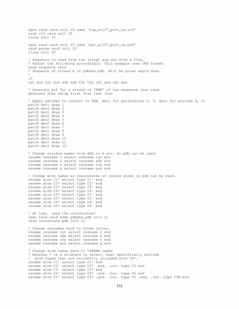
151

open read card unit 20 name "top_all27_prot_na.rtf" read rtf card unit 20 close unit 20 open read card unit 20 name "par_all27_prot_na.prm" read param card unit 20 close unit 20 ! Sequence is read from the script and not from a file. ! Adjust the following accordingly. This example uses CRD format. read sequence card * Sequence of strand A of pdbdna.pdb. Will be given segid dnaa * 12 cyt gua cyt gua ade ade thy thy cyt gua cyt gua ! Generate psf for a strand of “RNA” of the sequence just read generate dnaa setup first 5ter last 3ter ! Apply patches to convert to DNA, deo1 for pyrimidines C, T, deo2 for purines A, G. patch deo1 dnaa 1 patch deo2 dnaa 2 patch deo1 dnaa 3 patch deo2 dnaa 4 patch deo2 dnaa 5 patch deo2 dnaa 6 patch deo1 dnaa 7 patch deo1 dnaa 8 patch deo1 dnaa 9 patch deo2 dnaa 10 patch deo1 dnaa 11 patch deo2 dnaa 12 ! Change residue names from ADE to A etc. so pdb can be read. rename resname c select resname cyt end rename resname a select resname ade end rename resname t select resname thy end rename resname g select resname gua end ! Change atom names so coordinates of ribose atoms in pdb can be read. rename atom C1* select type C1' end rename atom C2* select type C2' end rename atom C3* select type C3' end rename atom C4* select type C4' end rename atom C5* select type C5' end rename atom O3* select type O3' end rename atom O4* select type O4' end rename atom O5* select type O5' end ! At last, read the coordinates! open read card name pdbdna.pdb unit 21 read coordinate pdb unit 21 ! Change resnames back to three letter. rename resname cyt select resname c end rename resname ade select resname a end rename resname thy select resname t end rename resname gua select resname g end ! Change atom names back to CHARMM names ! Because * is a wildcard in select, must specifically exclude ! atom types that are accidently included with CX*. rename atom C1' select type C1* end rename atom C2' select type C2* .and. .not. type C2 end rename atom C3' select type C3* end rename atom C4' select type C4* .and. .not. type C4 end rename atom C5' select type C5* .and. .not. type C5 .and. .not. type C5M end

152

rename atom O3' select type O3* end rename atom O4' select type O4* .and. .not. type O4 end rename atom O5' select type O5* end hbuild open write card name dnaout.pdb unit 31 write coordinate select all end pdb unit 31 * Output of roundabout way of handling DNA nomenclature * stop

Adding Counterions to DNA

Simulations and calculations including DNA are likely to be more accurate if the negatively charged phosphate groups are neutralized by counterions. Usually such ions are not present in the Protein Data Bank coordinate files of DNA, and they must be explicitly added. The following script shows one way of placing sodium ions halfway between the two oxygen atoms on each phosphate in a DNA strand. After such placement, energy minimization would, of course, be required to eliminate close encounters. During a dynamics simulation the sodium ions would be expected to move to still more appropriate positions.

The process begins by reading in the DNA and determining values for any coordinates that may be missing from the input file. A prototype sodium ion is then created and placed at the origin. After this, the script determines the residue number of the first phosphate present in the DNA and the total number of phosphates that are present. These values are used in the loop that adds the sodium ions. The counting operations use the selection capability of CHARMM. In addition to selecting atoms to be used in a command, select also sets the values of several substitution parameters. SELRESI is set to the residue number of the first atom that is selected, and NSEL is set to the number of atoms that are selected. Select must be used within a command, and here coordinate copy was chosen as an innocuous place in which to include the select command and therefore to have the required values place in SELRESI and NSEL.

The contents of the loop are patterned after the loops in the script discussed earlier that generates a box of water molecules. In the loop used here, each cycle through the loop creates a new sodium ion. This is first given the coordinates of the prototype sodium at the origin. Then the coordinates are determined where this sodium ion is to be placed. The sodium ion is placed at the midpoint of the vector from one of the phosphate oxygen atoms to the other oxygen atom. The midpoint is determined with the coordinate axis command. It places the midpoint of the vector from one of the phosphate oxygen atoms to the other in the substitution parameters XCEN, YCEN, and ZCEN. These values are added to the coordinates of the new sodium ion, and then the new sodium is placed in the same segment as the prototype sodium. The loop counter which determines to which phosphate a sodium is added to is then incremented. If it remains less than or equal to the last phosphate group, the loop is repeated. When all sodium ions have been added, the loop is exited and the same process is repeated for the other DNA strand. At the end, the prototype sodium is deleted and the coordinates are written out and can be viewed. * This file is counter.inp. * Usage, charmm <counter.inp >counter.out. * Adds sodium ions halfway between O1P and O2P oxygen atoms on phosphates of DNA. * Strands are assumed to have segment identifiers dnaa and dnab

153

* Input coordinate files to be output from inputdna.inp. * ! Open and read topology and parameter files. open read card unit 20 name "top_all27_prot_dna.rtf" read rtf card unit 20 close unit 20 open read card unit 21 name "par_all27_prot_na.prm" read parameter card unit 21 close unit 21 ! Read sequence and coordinates of DNA strands from files. open read card unit 22 name 1bnaa.pdb read sequence pdb unit 22 generate dnaa setup first 5ter last 3ter rewind unit 22 read coordinate pdb unit 22 close unit 22 ! Read second strand. open read card unit 23 name 1bnab.pdb read sequence pdb unit 23 generate dnab setup first 5ter last 3ter rewind unit 23 read coordinate pdb append unit 23 close unit 23 ! Add any missing atoms. ic fill preserve ic parameter ic build hbuild ! Create a prototype sodium ion at the origin. Its coordinates will be ! copied to new sodium ions. read sequence card * Sequence of Na+ * 1 sod generate sodp first none last none ! Append is needed so coordinates are applied to last residue listed in psf. read coordinate append card unit 5 * This is the title line followed by a blank line * 1 1 1 SOD SOD .00000 .00000 .00000 SODP 1 .00000 ! Count phosphates. Coordinate copy is just a dummy so that select can be ! used to count the phosphates. coordinate copy comp select segid dnaa .and. type P end ! Select command places the residue number of first selected atom in SELRESI ! and the number of selected atoms in NSEL. calculate phos = ?SELRESI calculate endno = ?SELRESI + ?NSEL -1 ! Loop for adding Na+ to first strand. ! Note that two loops are used and labels must be different from each other. label toploopa

154

! Create a sodium, soda, that will be placed near a phosphate. read sequence card * Sequence of Na+ * 1 sod ! Generate the segid "soda" generate soda setup first none last none noangle nodihedral ! Assign the coordinates of the prototype sodium to the new sodium. coordinate duplicate select segid sodp .and. resid 1 end select segid soda end ! Determine midpoint between atoms O1P and O2P. Coordinate axis command ! places the midpoints in XCEN, YCEN, ZCEN. coordinate axis select segid dnaa .and. resid @phos .and. type O1P end - select segid dnaa .and. resid @phos .and. type O2P end ! Add midpoint between phosphate oxygen atoms to sodium coordinates (origin). scalar x add ?XCEN select segid soda end scalar y add ?YCEN select segid soda end scalar z add ?ZCEN select segid soda end ! Add new sodium, soda, to existing ions, sodp. join sodp soda renumber increment phos by 1 if @phos le @endno goto toploopa ! To add Na+ to second strand, comments omitted. coordinate copy comp select segid dnab .and. type P end calculate phos = ?SELRESI calculate endno = ?SELRESI + ?NSEL -1 label toploopb read sequence card * Sequence of Na+ * 1 sod generate soda setup first none last none noangle nodihedral coordinate duplicate select segid sodp .and. resid 1 end select segid soda end coordinate axis select segid dnab .and. resid @phos .and. type O1P end - select segid dnab .and. resid @phos .and. type O2P end scalar x add ?XCEN select segid soda end scalar y add ?YCEN select segid soda end scalar z add ?ZCEN select segid soda end join sodp soda renumber increment phos by 1 if @phos le @endno goto toploopb ! Delete prototype sodium. delete atom select segid sodp .and. resid 1 end ! Write out coordinates of DNA and sodium ions. open write card name nadna.pdb unit 31 write coordinate select all end pdb unit 31

155

* DNA with sodium ions neutralizing each phosphate in strands dnaa and dnab * stop

156

Problems

1. Write a patch for the conversion of L-arabinose to L-ribulose.

2. Using the two entries in the residue topology file, write a patch for the conversion of alanine to aspartic acid. Note that all the angle and dihedral terms that involve any of the new atoms must be listed. The corresponding angle terms are absent in the residue topology file because the angle and dihedral terms needed in the psf are generated automatically as a result of the autogenerate angles dihedrals command that is near the beginning of the file. Apply your patch to an alanine residue in any protein and use a molecular graphics program, examine the angle between the two added oxygen atoms. Remove the angle term ANGLE OD1 CG OD2 from your patch and reexamine the angle between the oxygen atoms after application of the modified patch.

3. In many circumstances either the deo1 or deo2 patch can be applied to all the bases, both purines and pyrimidines. For what circumstances are the two patches not interchangeable?

4. Write a script and patch, if necessary, for the deletion of a nonterminal residue from a protein.

5. The example of pulling, the protein was in vacuum. Repeat the pulling exercise in the presence of implicit water and explicit water.

6. Write a script for the adjustment of Phi and Psi of any given residue in which the residue and the Phi and Psi values are passed to CHARMM from the command line invoking the program.

7. Write a script for adjusting Chi1 and Chi2 in the H80R mutant of AraC dimerization domain. Increment the angles in 10 amounts and energy minimize each structure to determine which rotameric state is the most probable. Use implicit water and the eef1 potentials.

8. Devise a script for the adjustment of Chi1 of an amino acid that performs the adjustment in real space. That is, do not use internal coordinates.

9. Write a script for joining two polypeptides when the C-terminal residue of the first polypeptide is proline, and do the same when it is glycine.

Bibliography

Canutescu, A. A., Shelenkov, A. A., and Dunbrack, R. L., Jr.(2003). A Graph-theory Algorithm for Rapid Protein Side-chain Prediction. Protein Sci. 12, 2001-2014.

Frenkel, D. and Smit, Berend, (1996). "Understanding Molecular Simulation From Algorithms to Applications," Academic Press, San Diego. An extensive theoretical background with some programming examples of the simulation of molecules and macromolecules in equilibrium.

Humphrey, W., Dalke, A. and Schulten, K. (1996). VMD - Visual Molecular Dynamics, J. Molec. Graphics 14, 33-38.

Lazaridis, T., and Karplus, M. (1999). Effective Energy Function for Proteins in Solution, Proteins 35, 133-152.

157

Leach, A. (2001). "Molecular Modeling, Principles and Applications, 2nd ed." Prentice Hall, Harlow, England. Thoroughly introduces and illustrates many techniques that are used in molecular modeling.

Merman, H. M., Westbrook, Z., Feng, G., Gilliland, G., Bhat, T. N., Wwissig, H., Shindyalov, I. N., Bourne, P. E. (2000). The Protein Data Bank, Nucleic Acids Res. 28, 235-242.

Paci, E., Vendruscolo, M., and Karplus, M. (2002). Native and Non-native Interactions Along Protein Folding and Unfolding Pathways, Proteins 47, 379-392.

Rapaport, D. (1995). “The Art of Molecular Dynamics Simulation,” Cambridge University Press, Cambridge. A molecular dynamics tutorial as well as containing a large number of relevant computer programs.

Schlick, T. (2002). “Molecular Modeling and Simulation, An Interdisciplinary Guide” Series: Interdisciplinary Applied Mathematics, Vol. 21, Springer, New York. A wide-ranging introduction to modeling.

Related Web Sites

http://www.charmm.org The official CHARMM site. Bulletin boards, forums, on a number of CHARMM related topics are moderated by noted CHARMM experts. The place to go for help with difficult problems.

http://www.psc.edu/general/software/packages/charmm/tutorial Tutorial lectures on molecular dynamics and a number of sophisticated and general CHARMM scripts.

http://mccammon.ucsd.edu/~chem215 A very complete description of the modeling of biological macromolecules.

http://www.lobos.nih.gov/Charmm The documentation for recent versions of CHARMM as well as useful links to CHARMM related material.

http://www.ks.uiuc.edu/Research/vmd/ Web site for the molecular display program VMD.

http://www.sinica.edu.tw/~scimath/msi/insight2K/charmm_principles/CHARMm_PrinTOC.doc.html Excellent source of information, but considerable understanding is necessary to make use of it.

http://xray.bmc.uu.se/hicup/ HIC-Up, The Hetero-compound Information Centre, much useful information for patch or resi construction for small molecules.

http://dunbrack.fccc.edu/Software.php A source of rotamer libraries and the program SCRWL for the prediction of rotameric states in proteins.

158

Appendices

System or CHARMM Modifications

Changing limits

The maximum number of lonepairs (MAXLP) and lonepair hosts (MAXLPH) can be specified in dimens.fcm. Upon recompilation, it's fine.

Command Line Substitution Parameters General:

'PI ' - Pi, 3.141592653589793 'KBLZ' - The Boltzmann factor (0.001987191) 'CCELEC' - 1/(4 PI epsilon) in AKMA units (332.0716) 'SPEEDL' - Speed of light 'CNVFRQ' - Conversion from root(Kcals/mol/AMU) to frequencies in CM-1. 'TIMFAC' - Conversion from AKMA time to picoseconds

Control and system variables:

'BOMLEV' - The error termination level (-5 to 5) 'WRNLEV' - The warning print level (-5 to 10) 'PRNLEV' - The standard print level (-1 to 15) 'IOLEV' - The I/O level (-1 to 1) 'IOSTAT' - The status of most recent OPEN command (-1=failed,1=OK) 'TIMER' - 'FASTER' - 'LFAST' - 'OLMACH' - 'OUTU' - 'FLUSH' - 'FNBL' - 'NBFACT' - 'LMACH' - 'MYNODE' - Current node number (0 to NUMNODE-1) 'NUMNODE' - The number of nodes (distributed memory) 'NCPU' - The number of CPUs (shared memory use) 'SYSSTAT' -

PSF counts

'NSEG' - Number of segments 'NRES' - Number of residues 'NATO' - Number of atoms 'NATOM' - "

159

'NGRP' - Number of groups 'NBON' - Number of bonds 'NBOND' - " 'NTHE' - Number of angles 'NTHETA' - " 'NPHI' - Number of dihedrals 'NIMP' - Number of improper dihedrals 'NIMPHI' - " 'NACC' - Number of acceptors 'NDON' - Number of donors 'NNB' - Number of explicit nonbond exclusions 'CGTOT' - Total system charge 'MASST' - Total system mass 'NATI' - Total number of image plus primary atoms

Parameter counts

'NATC' - Number of atom types 'NCB' - Number of bond parameters 'NCT' - Number of angle parameters 'NCSB' - Number of stretch-bend parameters 'NCP' - Number of diheral parameters 'NCI' - Number of improper dihedral parameters 'NCOOP' - Number of out-of-plane parameters 'NCH' - Number of hydrogen bond parameters 'NCN' - Number of vdw parameter pairs 'NCQ' - Number of bond charge increments

Other counts

'NCSP' - Number of restrained dihedral (CONS DIHE command). 'NTRA' - Number of image transformations 'TOTK' - Number of Ewald K vectors (not PME) 'NIC' - Number of Internal Coordinate entries in the IC table

Dimension Limits

'MAXA' - Number of atoms 'MAXATC' - Number of atom types 'MAXB' - Number of bonds 'MAXIMP' - Number of improper dihedrals 'MAXNB' - Number of explicit nonbond exclusions 'MAXP' - Number of dihedrals 'MAXPAD' - Number of donors and acceptors 'MAXRES' - Number of residues

160

'MAXSEG' - Number of segments 'MAXT' - Number of angles 'MAXCB' - Number of bond parameters 'MAXCH' - Number of hydrogen bond parameters 'MAXCI' - Number of improper dihedral parameters 'MAXCN' - Number of vdw pair parameters 'MAXCP' - Number of dihedral parameters 'MAXCT' - Number of angle parameters 'MAXCSP' - Number of restrained dihedrals

Coordinate manipulation parameters:

'XAXI' - vector and length of defined axis (COOR AXIS command). 'YAXI' 'ZAXI' 'RAXI' 'XCEN' - origin of axis vector 'YCEN' 'ZCEN' 'XMIN' - Extreme values (COOR STAT command) 'YMIN' 'ZMIN' 'WMIN' 'XMAX' 'YMAX' 'ZMAX' 'WMAX' 'XAVE' - Average values (COOR STAT command). 'YAVE' 'ZAVE' 'WAVE' 'MASS' - mass of selected atoms 'RMS' - Root mean squared difference between two structures. 'MASS' - mass (COOR ORIE and COOR RMS commands). 'XMOV' - displacement of atoms from best fit (COOR ORIE command). 'YMOV' - 'ZMOV' - 'XCEN' - 'YCEN' - 'ZCEN' - 'THET' - Angle of rotation from best fit 'AREA' - Requested surface area (COOR SURF command).

161

'VOLUME' - Requested volume (COOR VOLUme command). 'NVAC' - Number of vacuum points 'NOCC' - Number of occupied points 'NSEL' - Number of selected points 'FREEVOL'- Total free volume 'MIND' - Minimum distance (COOR MIND command). 'NPAIR' - Number of pairs (COOR DIST command). 'NCONTACT' - Number of contacts (COOR DMAT command). 'RGYR' - Radius of gyration (COOR RGYR command). 'XCM' - Center of mass (COOR RGYR command). 'YCM' - 'ZCM' - 'MASS' - Mass of selected atoms 'XDIP' - Dipole moment (COOR DIPOle command) 'YDIP' - 'ZDIP' - 'RDIP' - Dipole magnitude 'CHARGE'- Charge of selected atoms 'NHBOND' - total number of hydrogen bonds (COOR HBONd command). 'AVNOHB' - Average number of hydrogen bonds 'AVHBLF' - Average hydrogen bond life

SCALar STATistics command substitution parameters:

'SMIN' - Minimum value 'SMAX' - Maximum value 'SAVE' - Average value 'SVAR' - Variance about average 'SWEI' - Total weight used in the averaging 'STOT' - Total of selected atoms 'NSEL' - Number of selected atoms

Quick command substitution paramteters:

'XVAL' - X position of group of atoms 'YVAL' - X position of group of atoms 'ZVAL' - X position of group of atoms 'DIST' - Distance between two atom analysis 'THET' - Angle for three atom analysis 'PHI ' - Dihedral for four atom analysis

Shape analysis

'SFIT' - 'THET' -

162

'XAXI' - 'YAXI' - 'ZAXI' - 'RAXI' -

Saddle point calculation (TRAVel)

'SADE' - Saddle point energy 'SADI' - Saddle point index 'SADO' - Saddle point order

Energy calculation results:

'XCM' - Center of mass (from MMFP energy term calcuation) 'YCM' - 'ZCM' - 'XCM2' - Spatial extent 'YCM2' - 'ZCM2' - 'RGEO' - average distance from reference 'ENPB' - electrostatic free energy of solvation (from PBEQ) 'RMAX' - maximum distance to origin for the SSBP energy term

Minimization results:

'MINCONVRG' - 'MINECALLS' - 'MINGRMS' - 'MINSTEPS' -

PERT results:

'TPDEL' - Thermodynamic Perturbation energy change 'TPTOT' - Thermodynamic Perturbation total energy 'TIDEL' - Thermodynamic Integration energy change 'TITOT' - Thermodynamic Integration total energy 'SLDEL' - Slow Growth energy change 'SLTOT' - Slow Growth total energy

Atom selection parameters:

'NSEL' - Number of selected atoms from the most recent atom selection. 'SELATOM' - Atom number of first selected atom 'SELCHEM' - Chemical type of first selected atom 'SELIRES' - Residue number of first selected atom 'SELISEG' - Segment number of first selected atom 'SELRESI' - Resid of first selected atom 'SELRESN' - Residue type of first selected atom 'SELSEGI' - Segid of first selected atom

163

'SELTYPE' - Atom name of first selected atom

Crystal parameters

'XTLA' - Unit cell dimensions 'XTLB' - 'XTLC' - 'XTLALPHA' - Unit cell angles 'XTLBETA' - 'XTLGAMMA' - 'XTLXDIM' - Number of crystal degrees of freedom (cube=1,triclinic=6,..)

Data from most recently read (or current) trajectory file

'NFILE' - Number of frames in the trajectory file 'START' - Step number for the first frame 'SKIP' - Frequency at which frames were saved (NSTEP=NFILE*SKIP when not using restart files) 'NSTEP' - Total number of steps in the simulation 'NDEGF' - Number of degrees of freedom in the simulation (Can be use to get the temperature with velocity files). 'DELTA' - The dynamics step length (in picoseconds).

Nonbond list counts

'NNBA' - Number of atom pairs (main list) 'NNBG' - Number of group pairs (main list) 'NNBI' - Number of crystal atom pairs (Phonons only) 'NRXA' - Number of atom exclusions due to replicas 'NRXG' - Number of group exclusions due to replicas

Correlation Function Results

'AVER' - Series average (CORREL's SHOW command) 'FLUC' - Series fluctuation 'P2' - P2 average 'P2R3' - 'P2RA' - 'R3R' - 'R3S' - 'P0' - Polynomial best fit components (MANTime POLY command). 'P1' - 'P2' - 'P3' - 'P4' - 'P5' - 'P6' -

164

'P7' -

Vibrational analysis of thermodynamic properties:

'FTOT' - Vibrational free energy. 'STOT' - Vibrational entropy. 'HTOT' - Vibrational enthalpy. 'CTOT' - Vibrational heat capacity. 'ZTOT' - Zero point correction energy. 'FCTO' - Classical vibrational free energy. 'ETOT' - Total harmonic limit classical free energy (to compare with free energy perturbation simulations). 'TRAC' - Trace of the Hessian for selected atoms

Miscellaneous:

'VIOL' - Total violation for all NOE restraints (NOE WRITe/PRINt ANAL) 'DRSH' - the DRSH value in subroutine PSHEL (undocumented) (also undocumented in fcm/mmfp.fcm in violation of coding stds.) 'DCOEFF'- The diffusion constant (COOR ANALysis SOLVent command). 'TIME' - simulation time(ps) for current frame in trajectory reading 'STEP' - Step number for current frame in trajectory reading

Energy related properties:

'TOTE' - total energy 'TOTK' - total kinetic energy 'ENER' - total potential energy 'TEMP' - temperature (from KE) 'GRMS' - rms gradient 'BPRE' - boundary pressure applied 'VTOT' - total verlet energy (no HFC) 'VKIN' - total verlet kinetic energy (no HFC) 'EHFC' - high frequency correction energy 'EHYS' - slow growth hysteresis energy correction 'VOLU' - the volume of the primitive unit cell = A.(B x C)/XNSYMM. Defined only if images are present, or unless specified with the VOLUme keyword. 'PRSE' - the pressure calculated from the external virial. 'PRSI' - the pressure calculated from the internal virial. 'VIRE' - the external virial. 'VIRI' - the internal virial. 'VIRK' - the virial "kinetic energy". Energy term names: 'BOND' - bond (1-2) energy

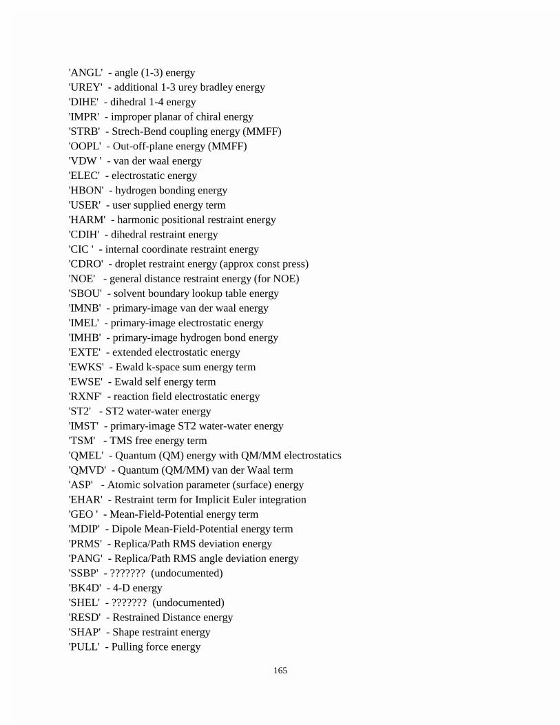
165

'ANGL' - angle (1-3) energy 'UREY' - additional 1-3 urey bradley energy 'DIHE' - dihedral 1-4 energy 'IMPR' - improper planar of chiral energy 'STRB' - Strech-Bend coupling energy (MMFF) 'OOPL' - Out-off-plane energy (MMFF) 'VDW ' - van der waal energy 'ELEC' - electrostatic energy 'HBON' - hydrogen bonding energy 'USER' - user supplied energy term 'HARM' - harmonic positional restraint energy 'CDIH' - dihedral restraint energy 'CIC ' - internal coordinate restraint energy 'CDRO' - droplet restraint energy (approx const press) 'NOE' - general distance restraint energy (for NOE) 'SBOU' - solvent boundary lookup table energy 'IMNB' - primary-image van der waal energy 'IMEL' - primary-image electrostatic energy 'IMHB' - primary-image hydrogen bond energy 'EXTE' - extended electrostatic energy 'EWKS' - Ewald k-space sum energy term 'EWSE' - Ewald self energy term 'RXNF' - reaction field electrostatic energy 'ST2' - ST2 water-water energy 'IMST' - primary-image ST2 water-water energy 'TSM' - TMS free energy term 'QMEL' - Quantum (QM) energy with QM/MM electrostatics 'QMVD' - Quantum (QM/MM) van der Waal term 'ASP' - Atomic solvation parameter (surface) energy 'EHAR' - Restraint term for Implicit Euler integration 'GEO ' - Mean-Field-Potential energy term 'MDIP' - Dipole Mean-Field-Potential energy term 'PRMS' - Replica/Path RMS deviation energy 'PANG' - Replica/Path RMS angle deviation energy 'SSBP' - ??????? (undocumented) 'BK4D' - 4-D energy 'SHEL' - ??????? (undocumented) 'RESD' - Restrained Distance energy 'SHAP' - Shape restraint energy 'PULL' - Pulling force energy

166

'POLA' - Polarizable water energy 'DMC ' - Distance map restraint energy 'RGY ' - Radius of Gyration restraint energy 'EWEX' - Ewald exclusion correction energy 'EWQC' - Ewald total charge correction energy 'EWUT' - Ewald utility energy term (for misc. corrections)

Energy Pressure/Virial Terms:

'VEXX' - External Virial 'VEXY' - 'VEXZ' - 'VEYX' - 'VEYY' - 'VEYZ' - 'VEZX' - 'VEZY' - 'VEZZ' - 'VIXX' - Internal Virial 'VIXY' - 'VIXZ' - 'VIYX' - 'VIYY' - 'VIYZ' - 'VIZX' - 'VIZY' - 'VIZZ' - 'PEXX' - External Pressure 'PEXY' - 'PEXZ' - 'PEYX' - 'PEYY' - 'PEYZ' - 'PEZX' - 'PEZY' - 'PEZZ' - 'PIXX' - Internal Pressure 'PIXY' - 'PIXZ' - 'PIYX' - 'PIYY' - 'PIYZ' -

167

'PIZX' - 'PIZY' - 'PIZZ' -

168

Index

a

-, 43, 139 CHARMM long line continuation, 43 Preceding residue, 17

'

', 78, 147

!

!, 17 CHARMM comment, 17

"

", 119

#

#, 26

$

$X. See awk

%

%, 26

&

&, 27

*

*, 26, 147

.

., 7

.., 7

./, 7

/

/, 2 /dev/tty, 78

:

:, 26 :Linux long line continuation, 119

?

?, 22, 59. See Substitution parameters substitution parameter value, 22

@

@, 29, 59, 129 variable value, 59

+

+, 26, 139 Following residue, 17

++, 39, 85 +=, 58

<

<. See Linux redirection

A

ABNR, 93 Accessible surface, 54 Accessible surface area, 56 Acetylate terminus, 137 Alpha helix, 49, 82, 129 Alternative conformation, 34 Angle determination, 49 Append, 63 Archive file, 5 Area of interface, 79 Array, 15, 22, 61

wcomp, 59 Arrays, 125 ASP, 97 Asymmetric unit, 71 Atom

adding, 138 creating, 138 deleting, 138 identifier, 139 name, 147

Atom name, 147 Atom property, 26 Atom selection, 26 Atom type, 15, 17, 36 Awk. See Linux commands Awk commands

BEGIN, 38

169

command line argument, 38 FIELDWIDTHS, 38 substring, 39

Awk examples, 50, 57, 73, 94, 105, 119, 147

B

B value, 18, 71 Backbone selection, 25 Background

running in, 27 Bash shell, 6 Beta sheet, 49, 129 Binary, 44 Binary format, 44 Biological molecule, 71 Biomolecule, 71 Bomb. See CHARMM crash Bomb level, 30 Bond bending, 10 Bond strength, 17 Bond stretching, 10 Bond twisting, 10 Bonding pattern, 19 Boolean logic, 26

C

C shell, 6 Cannot open file, 45 Carboxyl terminal oxygen, 40 Card, 44 Card format, 44 Carriage return, 28 Cartesian coordinates, 40

constructing, 129 Case sensitivity, 45 Cavity, 60 CD1, 35 Change name, 133 Character count, 28 CHARMM

abbreviations, 43 atom type, 16 command line substitution, 117 comment, 17 comparison operators, 30, 59 crash, 28, 29, 30, 40, 45, 63, 98, 110, 112, 113,

114, 118, 122, 125, 137 dynamics, 110 energy, 117 exclamation mark, 17 license, 5

looping, 117 number limits, 125 output, 44, 45, 46 passing parameters, 29 residue limits, 125 test cases, 5 trajectory, 116

Charmm commands generate, 41, 63 hbuild, 42 ic build, 42

CHARMM commands append, 63 autogenerate, 138, 139 bomb, 30 calculate, 59 coordinate axis, 152 coordinate duplicate, 67, 88, 125 coordinate initialize, 136 coordinate orient, 66, 88, 94, 109 coordinate read, pdb, 43 coordinate rotate, 73 coordinate search, 60 coordinate set, 132 coordinate translate, 73, 125, 129, 132 crystal, 114 dynamics, 100, 105 first none, 142 generate, 117, 129, 137 generate setup, 128, 137 goto, 59 hbuild, 43, 106, 144 ic build, 43, 129, 138 ic edit, 136 ic fill, 144 ic parameter, 43 ic seed, 129 if, 30 install, 6 iread, 116 join, 127, 129 label, 59 last none, 142 long line continuation, 43 minimization, 93 minimize, 94, 105 noangle, 128 nodihedral, 128 offset, 63 open read, 43 open read pdb, 43, 45 open write, 84 open write, psf, 44 print, 144

170

prnlev, 30 read parameter file, 43 read rtf file, 43 read sequence, 128, 129 read sequence, pdb, 43, 45 rename, 129, 133, 150 scalar, 57, 59 scalar add, 125 scalar statistics, 80 select ires, 64 set, 59, 129 shake, 99 skip, 116 syntax, 53 trajectory, 120 trajectory iread, 116 trajectory query, 116, 117 trajectory read, 116 wrnl, 30

Chi angles, 135 Clock speed, 1 Coiled-coil, 77 Comma separated columns, 85 Comma separated values, 85 Comma separated variables, 58 Command line argument, 38 Command line interface, 3 Command line parameters, 29 Command parsing, 7 Command prompt, 3 Comments

CHARMM, 44 Comparison array, 53 Comparison coordinate set, 15 Comparison operators, 26 Conformation changes, 87 Constant pressure, 101 Constant temperature, 101 Constraints, 131 Contact map, 82 Contact surface, 55 Coordinate

array, 53 dmat, 84 duplicate, 67 ic edit, 136 initialize, 136 internal, 43 manipulation, 53 orient, 66 pdb, 34, 119 read, 116 read crd, 128

read pdb, 43, 128 rotation matrix, 73 translate, 73 write crd, 44 write pdb, 44, 150

Coordinate rotate, 73 Coordinates

Cartesian, 8 internal, 8, 15 limits, 75

Correlation function, 120 Counterion, 152 Counting, 152 Crash. See CHARMM crash crd, 19 Creating a new molecule, 125 Creating ions, 152 Crystal lattice, 71 Crystallographic B value, 71 Crystallographic water, 101 CSV. See comma separated variables CTER, 141 C-terminal oxygens, 36 Cutoff distance, 13

D

dcd, 116 dcd files, 116 Default parameter values, 13 Delete atoms, 108, 109, 133 Deoxy, 87 Deoxyribonucleotide, 147 Dielectric constant, 13 Dihedral angle, 11, 135, 136 Dimerization interface, 79 Dipole-dipole interaction, 13 Directory, 2 Distance difference map, 87 Distance matrix, 82 Disulfide bond, 137 dmat, 84 DNA, 146

from RNA, 150 Documentation, 4, 8 Dummy atom, 61

E

eef1, 113 Electrostatic forces, 13, 17 Electrostatic interactions, 17, 139

171

Energy, 97, 117 minimization, 132

Energy minimization, 93, 95, 100 Energy terms, 138

dihedral, 139 output, 96

Equilibration, 100 Error messages, 30 Ewald, 114 Ewald approximation, 101 Extracting data. See Linux commands grep

F

Fieldwidths, 37, 38 File format, 44

tar, 5 Finding files, 5 Finding words, 5 Fixing atoms, 131 Fluctuations, 110 Force arrays, 22 Format

new line, 79 Formatted printing, awk, 74 Frame, 116 Frictional forces, 112

G

GFP, 138 Glucose, 140 Glycine, 49, 137 GNU, 122 Green fluorescent protein, 138 Grep examples, 5, 57, 84 GRMS, 96 Group, 17, 139

H

Handling ligands, 137 Handling patches, 137 Harmonic potential, 131 HBOND, 97 Heating, 110 Heating systems, 100 Hemoglobin, 87 Hetatom, 36 Histidine, 35 Hole, 60 HSD. See Histidine

HSE. See Histidine Html, 8 Hydrogen bond, 143 Hydrogen bonds, 13 Hydrogen vibration, 98

I

IC, 43 Improper dihedral angle, 10, 95 Index loop counter. See CHARMM commands,

increment Initialize coordinates, 41 Instabilities, 100 Install, 6 Interaction energy, 117 Internal coordinates, 16, 40, 43, 49, 135. See

Coordinates, internal Internet browser, 8 Ion

sodium, 152 Ires, 19, 24, 64 IUPAC, 18

L

Langevin, 99, 112 L-arabinose, 140 Lattice transformations, 76 Lennard-Jones potential, 12 Ligand, 63 Ligands

handling, 137 Line continuation, 43, 119 Linux commands

", 119 &, 27 awk, 4, 38, 119 cd, 3 cp, 3 csh, 6 df, 28 du, 28 echo, 6, 79 editor, 43 exit, 6 find, 5 gedit, 43 grep, 4, 5, 57, 84 head, 28 kill, 28 ls, 3 man, 3

172

mkdir, 3 more, 28, 45 nice, 28 nohup, 27 redirection, 38, 43 rm, 3 tail, 28 tar, 5 tee, 28 top, 27 tr, 28 vim, 43 wc, 28

Long lines, 43, 119 Looping, 58, 117, 129, 152

M

Main coordinate set, 15 Matrix, 82 Minimization, 95, 100

energy, 93, 132 Missing atoms, 40, 143 Missing coordinates, 40 Model construction, 125 Mount CD, 6 Moving a molecule, 125 Multiple coordinate sets, 63 Multiple subunits, 63 Mutation, 133

N

Name change, 150 NBONDX, 107 New line, 28 Newton's equation of motion, 13 Newtwon-Raphson, 93 Noangle, 106 Nodihedral, 106 Nonbonded interactions, 17 Nonbonded list, 13, 17, 93, 95, 114 NTER, 141 N-terminus, 137

glycine, 137 proline, 137

Nucleic acid, 146

O

OCT, 36 Open read, 44 Open write, 44

Output redirection, 78 Output verbosity, 30 OXT, 36 Oxy, 87

P

Parameter file, 15, 93 Parameter files, 17, 139 Parameter table, 13, 42 Partial charge, 17, 133, 142 Partial charges, 139 Passing information, 29 Passing parameters, 29, 129, 132, 133 Passing variables, 129 Patch, 147

DNA, 149 Patches, 46, 133, 137, 138, 141, 156 Path, 6 PBC, 99 pdb, 18, 34, 73 Peptide chain

discontinuous, 63 Peptides

linking, 144 Periodic boundary conditions, 99 Phi, 48, 129 Placing ions, 152 Polyproline helix, 49, 129 Potential

harmonic, 131 Potential field, 9 PRES, 138 Principal structure file, 15. See psf Print level, 30 printf, 74 Printf, 39, 85 Proline, 137 Proline issues, 133 psf, 19, 108, 117 Psi, 48, 129 Pulling atoms, 131

Q

Quantum mechanics, 13 Quotes, 119 Quotes, conversion protection, 45

R

Radius

173

atom, 61 Ramachandran plot, 48 Read

parameter, 144 trajectory, 117

Reading trajectories, 116 Redirection, 42, 79 Rename, 133 RESI, 140 Resid, 19, 24, 64 Residue limits, 125 Residue numbering, 63 Residue topology file, 15 Restart files, 112 Restarting dynamics, 100 Restraints, 131 Rewind, 63 Ribonucleotide, 147 Ribose, 140 RMS overlaying, 67, 88 RNA, 146 Root, 2 Root directory, 2 Root user, 6 Rotamer, 119, 135 Rotation, 108 Rotation matrix, 73, 74 rtf, 15, 44, 140, 147 Run string parameters, 29 Running programs, 6

S

Scalar array, 61 Scalar arrays, 22, 71 Script, 1, 5, 7, 42 Searching for data. See grep Segid, 19, 24, 45 Segment identifier, 110 Select, 30, 59

all, 24 backbone, 25 ires, 64 resid, 64 residue, 24 residues nearby, 25 side chain, 25 to count, 152

Shell, 6 Side chain, 133 Side chain selection, 25 Skull and crossbones, 47

Sodium ion, 152 Solvent exposure, 56 Spreadsheet, 85 Step time, 97 Stereo graphics, 55 String, 39 Substitution parameter, 59 Substitution parameters, 22, 79, 152 Substring, 37, 39, 74 Surface area, 56, 79 Swap space, 122 Symmetry operations, 71

T

Tar, 5 Taylor series, 14 Temperature, 100 Test script, 5 Time series, 120 TIP3, 36, 128 Title lines, 47 Token, 59 Topology file. See rtf Total energy, 97 Trajectory, 13, 116, 120 Trajectory files, 117 Translation, 108 Translation matrix, 73

U

Unit cell, 76 Unit numbers, 44, 128 Units, 27 Unix, 37. See Linux USER, 97

V

Van der Waals forces, 12 Van der Waals interactions, 10, 17 Van der Waals radius, 61 Variable, 59, 119. See Substitution parameters Verlet, 14 VMD, 2, 129, 142

W

Water, 36, 128 box, 101 box of molecules, 125 drop, 108

174

implicit, 112 implicit and explicit, 99

Water drop, 99, 101 Wcomp, 59 Weight array, 22, 57, 71 Wildcard specifications, 26 wmain, 80 Wmain, 57

wmain array, 61 Word count, 28 Write

array, 59 coordinates, pdb, 44, 150 internal coordinates, 49 psf, 44

Write level, 30