civil engineering systems cee218b - faculty of engineering · civil engineering systems slobodan p....
TRANSCRIPT

The University of Western Ontario Department of Civil and Environmental Engineering
Civil Engineering Systems CEE218b
Course notes
Nile add
Other Resources
Resources
add to 1
add to 2
Nile inc
Res 2 inc
Resource 2 Development
Resource 1 Development
T3 plan
Upper Nile Projects
Other Res Dev Plan
Nile
HAD Release
Slobodan P. Simonovic, Ph.D., P.Eng.
Professor and Research Chair
London, December 2003
© Slobodan P. Simonovic

Civil Engineering Systems Slobodan P. Simonovic
2
PREFACE
This updated set of notes is prepared to serve as a supporting text for an introductory systems course for civil engineers. The text is not intended to be an independent document. Rather, it is to be used as a supplement to the instructor's lectures. This text, and the course upon which it is based, is designed to provide the students with the basic concepts of systems analysis and design using simulation and optimization. The course is aimed at the second year Civil Engineering students. During the past four decades, application of the systems approach to engineering systems design and management has been established as one of the most important advances made in the field of Civil Engineering. A primary emphasis of systems analysis is on providing an improved basis for decision making. It has been concluded that a gap still exists between research studies and the application of systems approach in practice. The objective of this course is to help in providing better communication links between different sub-disciplines of Civil Engineering and reduce the existing gap as much as possible. While some theoretical aspects are addressed, the course focuses primarily on analytical topics: various problems in civil engineering are presented; the problems are formulated as systems; and techniques are introduced with which to solve the systems. In an effort to provide the students with a complete tutorial package that aids in the formulation of the model, in the selection of the most appropriate technique, and in the implementation of the algorithm, exposure to two software packages, for system simulation and optimization, is planned. The general objectives of the course are for students to be able to:
• Use systems thinking in addressing engineering problems by understanding: system structure; links and interrelationships between different elements of the structure; feedback; and behaviour of systems over time.
• Understand and use the mathematical model as a device for formalization, standardization and treatment of engineering design and management problems.
• Improve communication skills by formulating, selecting appropriate solution methodology for, solving and presenting engineering design and management decisions based on the implementation of systems analysis.
• Develop an awareness of the potential utility of systems approach to Civil Engineering.
• Recognize the need for life -long learning, interdisciplinarity and use of the systems approach in Civil Engineering as one way for addressing comple xity.
Slobodan P. Simonovic, Ph.D., P.Eng. London, December 2003

Civil Engineering Systems Slobodan P. Simonovic
3
TABLE OF CONTENT PREFACE 2 TABLE OF CONTENT 3 1. INTRODUCTION 5 1.1 Principles of systems thinking 5 1.2 Open and feedback system 7 1.3 Patterns of behavior 9 1.4 Causal loop diagrams 11 1.5 Positive- reinforcing feedback loop 14 1.6 Negative – balancing feedback loop 15 1.7 Complex system behaviour 16 1.8 Creating causal loop diagrams 20 1.9 Problems 21 1.10 References 23 2. SYSTEMS ANALYSIS 24 2.1 Definitions 25 2.2 Systems approach 27 2.3 Systems engineering 32 2.4 Mathematical modelling 34 2.5 Classification of mathematical models and optimisation techniques 37 2.6 Problems 39 2.7 References 43 3. SYSTEM SIMULATION 44 3.1 Introduction 44 3.2 System Dynamics simulation approach for Civil Engineering problems 46 3.3 Basic building blocks of system dynamics simulation environments 48 3.4 System dynamics modelling process 52 3.5 Fundamental structures and behaviors 54 3.6 An engineering system dynamics model example 58 3.7 Problems 72 3.8 References 74 Appendix A Vensim quick tutorial 75 4. OPTIMIZATION BY CALCULUS 96 4.1 Introduction 96 4.2 Unconstrained functions 102 4.3 Constrained optimisation 107 4.4 Problems 111 4.5 References 114 5. LINEAR PROGRAMMING (LP) 115 5.1 What is linear programming? 115

Civil Engineering Systems Slobodan P. Simonovic
4
5.2 Canonical forms for linear optimisation models 119 5.3 Geometric interpretation 120 5.4 Simplex method of solution 124 5.5 Completeness of the Simplex algorithm 130 5.6 Duality in LP 133 5.7 Sensitivity analysis 136 5.8 Summary LP 160 5.0 Use of Microsoft Excel for solving linear programming problems 161 5.10 Problems 167 5.11 References 171 6. MULTIOBJECTIVE ANALYSIS 172 6.1 Basic concepts of multiobjective analysis 172 6.2 Multiobjective analysis – application examples 182 6.3 The weighting method 186 6.4 Problems 193 6.5 References 200 ABOUT THE AUTHOR 203
Civil Engineering Systems Slobodan P. Simonovic
5
1. INTRODUCTION
Human beings are quick problem solvers. From an evolutionary standpoint, quick
problem solvers were the ones who survived. We quickly determine a cause for any event
that we think is a problem. Usually we conclude that the cause is another event. For
example, if sales are poor (the event that is a problem), then we may conclude that this is
because the sales force is insufficiently motivated (the event that is the cause of the
problem). This approach works well for simple problems, but it works less well as the
problems get more complex.
1.1 Principles of Systems Thinking
The methods of systems thinking provide us with tools for better understanding these
difficult management problems. The methods have been used for over thirty years
(Forrester 1961 - 1990) and are now well established. However, these approaches require
a shift in the way we think about the performance of an organization. In particular, they
require that we move away from looking at isolated events and their causes (usually
assumed to be some other events), and start to look at the organization as a system made
up of interacting parts.
We use the term system to mean an interdependent group of items forming a unified
pattern. Since our interest here is in engineering, we will focus on systems of people and
technology intended to plan, design, construct and operate engineering infrastructure.
Almost everything that goes on in engineering is part of one or more systems. As noted
above, when we face a management problem we tend to assume that some external event
caused it. With a systems approach, we take an alternative viewpoint - namely that the
internal structure of the system is often more important than external events in generating
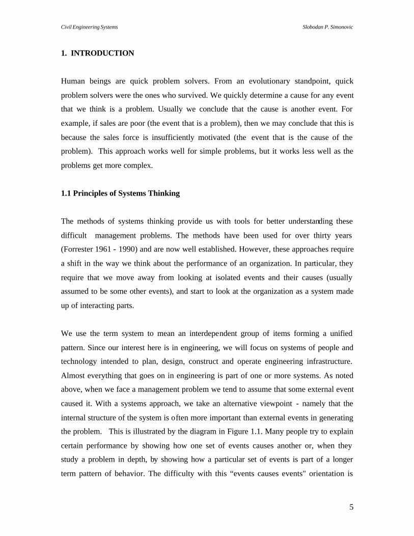
the problem. This is illustrated by the diagram in Figure 1.1. Many people try to explain
certain performance by showing how one set of events causes another or, when they
study a problem in depth, by showing how a particular set of events is part of a longer
term pattern of behavior. The difficulty with this “events causes events" orientation is
Civil Engineering Systems Slobodan P. Simonovic
6
that it doesn't lead to very powerful ways to alter the undesirable performance. You can
continue this process almost forever, and thus it is difficult to determine what to do to
improve performance.
Figure 1.1 Looking for problem solution (high leverage)
If you shift from this event orientation to focusing on the internal system structure, you
improve your possibility of finding the problem. This is because system structure is often
the underlying source of the difficulty. Unless you correct system structure deficiencies,
it is likely that the problem will resurface, or be replaced by an even more difficult
problem.
Class exercise 1:
- Automobile is a __ of components that work together to provide transportation.
- Autopilot is a __ for flying an airplane at a specific altitude.
- Loading platform is a __ for loading goods into trucks.

Civil Engineering Systems Slobodan P. Simonovic
7
- Management is a __ of people for allocating resources and regulating the activity of a
business.
- Family is a __ for living and raising children.
1.2 Open and Feedback System
An open system is one characterized by outputs that respond to inputs but where the
outputs are isolated from and have no influence on the inputs (Figure 1.2). An open
system is not aware of its own performance. In an open system, past action does not
control future action (Forester, 1990).
Figure 1.2 Graphical presentation of an open system
A feedback system (sometimes called a closed system) is influenced by its own past
behavior. A feedback system has a closed loop structure that brings results from past
action of the system back to control future action (Figure 1.3). One class of feedback
system -negative feedback- seeks a goal and responds as a consequence of failing to
achieve the goal. A second class of feedback system - positive feedback- generates
growth process wherein action builds a result that generates still greater action.
A broad purpose may imply a feedback system having many components. But each
component can itself be a feedback system in terms of some subordinate purpose. One
must then recognize a hierarchy of feedback structures where the broadest purpose of
interest determines the scope of the pertinent system. It is in the positive feedback form
of system structure that one finds the forces of growth. It is in the negative feedback, or
goal seeking, structure of systems that one finds the causes of fluctuation and instability.
System Input Output

Civil Engineering Systems Slobodan P. Simonovic
8
Figure 1.3 Graphical presentation of a feedback system
Another basic concept is the feedback loop. The feedback loop is a closed path
connecting in sequence a decision that controls action, the level (a state or condition) of
the system, and information about the level of the system (Figure 1.4). The single loop
structure is the simplest form of feedback system. There may be additional delays and
distortions appearing sequentially in the loop. There may be many loops that
interconnect. When reading a feedback loop diagram, the main skill is to see the ‘story’
that the diagram tells: how the structure creates a particular pattern of behavior and how
that pattern might be influenced.
Figure 1.4 A feedback loop
system level decision
action
System Input Output
Feedback

Civil Engineering Systems Slobodan P. Simonovic
9
Class exercise 2:
-The parts of a feedback system form a structure shaped as a (chain/loop)__.
-The ‘action’ represents the flow of something that is controlled by the __ .
-The __ alters the __ of the system.
- The __ of the system is the true condition of the system and is the source of information
about the system.
-The recurring __ governing the release of water from the reservoir changes as our
available __ about demand, inflow, and storage changes.
1.3 Patterns of Behavior
To start to consider system structure, you first generalize from the specific events
associated with your problem to considering patterns of behavior that characterize the
situation. Usually this requires that you investigate how one or more variables of interest
change over time (for example: flow of water; load on the bridge; wind load; etc.). That
is, what patterns of behavior do these variables display. The systems approach gains
much of its power as a problem solving method from the fact that similar patterns of
behavior show up in a variety of different situations, and the underlying system structures
that cause these characteristic patterns are known. Thus, once you have identified a
pattern of behavior that is a problem, you can look for the system structure that is know
to cause that pattern. By finding and modifying this system structure, you have the
possibility of permanently eliminating the problem pattern of behavior.
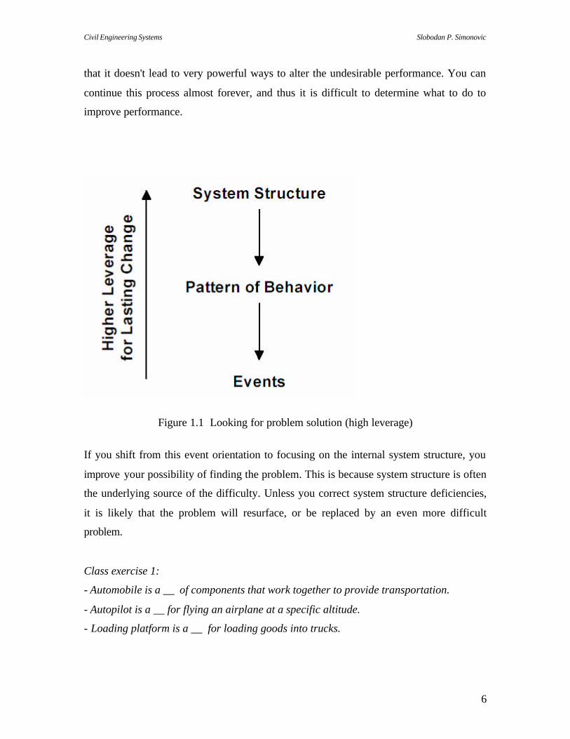
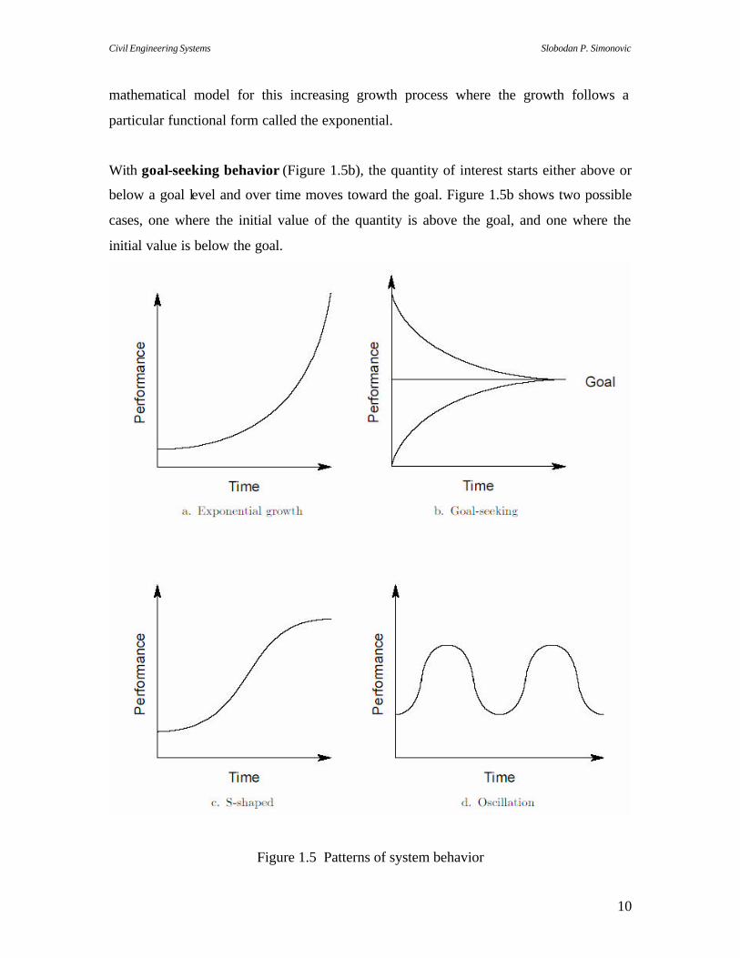
The four patterns of behavior shown in Figure 1.5 often show up, either ind ividually or in
combinations, in systems. In this figure, “Performance" refers to some variable of
interest.
With exponential growth (Figure 1.5a), an initial quantity of something starts to grow,
and the rate of growth increases. The term exponential growth comes from a
Civil Engineering Systems Slobodan P. Simonovic
10
mathematical model for this increasing growth process where the growth follows a
particular functional form called the exponential.
With goal-seeking behavior (Figure 1.5b), the quantity of interest starts either above or
below a goal level and over time moves toward the goal. Figure 1.5b shows two possible
cases, one where the initial value of the quantity is above the goal, and one where the
initial value is below the goal.
Figure 1.5 Patterns of system behavior
Civil Engineering Systems Slobodan P. Simonovic
11
With s-shaped growth (Figure 1.5c), initial exponential growth is followed by goal-
seeking behavior which results in the variable leveling of.
With oscillation (Figure 1.5d), the quantity of interest fluctuates around some level. Note
that oscillation initially appears to be exponential growth, and then it appears to be s-
shaped growth before reversing direction.
Common combinations of these four patterns include:
• Exponential growth combined with oscillation. With this pattern, the general trend
is upward, but there can be declining portions, also.
• Goal-seeking behavior combined with an oscillation whose amplitude gradually
declines over time. With this behavior, the quantity of interest will overshoot the
goal on first one side and then the other. The amplitude of these overshoots
declines until the quantity finally stabilizes at the goal.
• S-shaped growth combined with an oscillation whose amplitude gradually
declines over time.
1.4 Causal Loop Diagrams
To better understand the system structures which cause the patterns of behavior discussed
in the preceding section, we introduce a notation for representing system structures.
When an element of a system indirectly influences itself in the way discussed in section
1.2 the portion of the system involved is called a feedback loop or a causal loop.
The essence of the discipline of systems thinking lies in a shift of mind:
• seeing interrelationships rather than linear cause-effect chains; and
• seeing processes of change rather than snapshots.
To illustrate the shift consider a very simple system - filling a glass of water. You can
think that is not a system, it is too simple. From the linear point of view:
I am filling a glass of water.
Civil Engineering Systems Slobodan P. Simonovic
12
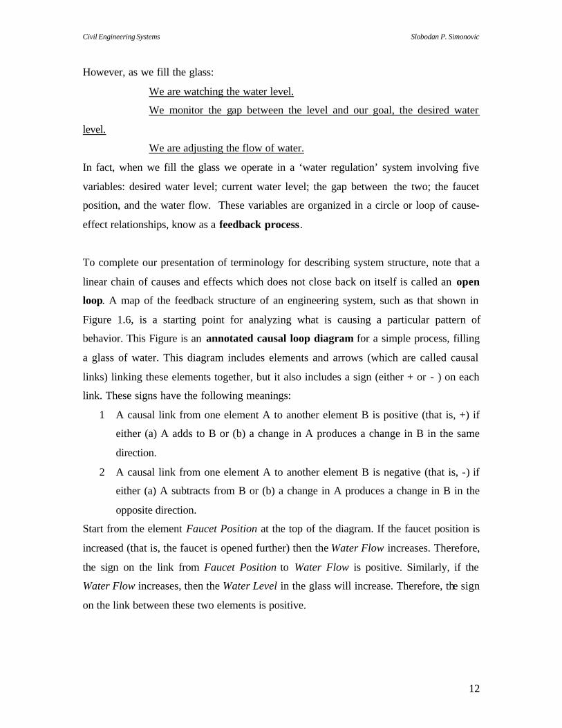
However, as we fill the glass:
We are watching the water level.
We monitor the gap between the level and our goal, the desired water
level.
We are adjusting the flow of water.
In fact, when we fill the glass we operate in a ‘water regulation’ system involving five
variables: desired water level; current water level; the gap between the two; the faucet
position, and the water flow. These variables are organized in a circle or loop of cause-
effect relationships, know as a feedback process.
To complete our presentation of terminology for describing system structure, note that a
linear chain of causes and effects which does not close back on itself is called an open
loop. A map of the feedback structure of an engineering system, such as that shown in
Figure 1.6, is a starting point for analyzing what is causing a particular pattern of
behavior. This Figure is an annotated causal loop diagram for a simple process, filling
a glass of water. This diagram includes elements and arrows (which are called causal
links) linking these elements together, but it also includes a sign (either + or - ) on each
link. These signs have the following meanings:
1 A causal link from one element A to another element B is positive (that is, +) if
either (a) A adds to B or (b) a change in A produces a change in B in the same
direction.
2 A causal link from one element A to another element B is negative (that is, -) if
either (a) A subtracts from B or (b) a change in A produces a change in B in the
opposite direction.
Start from the element Faucet Position at the top of the diagram. If the faucet position is
increased (that is, the faucet is opened further) then the Water Flow increases. Therefore,
the sign on the link from Faucet Position to Water Flow is positive. Similarly, if the
Water Flow increases, then the Water Level in the glass will increase. Therefore, the sign
on the link between these two elements is positive.

Civil Engineering Systems Slobodan P. Simonovic
13
The next element along the chain of causal influences is the Gap which is the difference
between the Desired Water Level and the (actual) Water Level. (That is, Gap = Desired
Water Level - Water Level.) From this definition, it follows that an increase in Water
Level decreases Gap, and therefore the sign on the link between these two elements is
negative. Finally, to close the causal loop back to Faucet Position, a greater value for
Gap presumably leads to an increase in Faucet Position (as you attempt to fill the glass)
and therefore the sign on the link between these two elements is positive. There is one
additional link in this diagram, from Desired Water Level to Gap. From the definition of
Gap given above, the in influence is in the same direction along this link, and therefore
the sign on the link is positive.
Figure 1.6 Causal loop diagram for ‘filling a glass of water’

Civil Engineering Systems Slobodan P. Simonovic
14
In addition to the signs on each link, a complete loop also is given a sign. The sign for a
particular loop is determined by counting the number of minus (-) signs on all the links
that make up the loop. Specifically, (i) A feedback loop is called positive, indicated by a
+ sign in parentheses, if it contains an even number of negative causal links; and (ii) A
feedback loop is called negative, indicated by a sign in parentheses, if it contains an odd
number of negative causal links.
Thus, the sign of a loop is the algebraic product of the signs of its links. Often a small
looping arrow is drawn around the feedback loop sign to more clearly indicate that the
sign refers to the loop, as is done in Figure 1.6. Note that in this diagram there is a single
feedback (causal) loop, and that this loop has one negative sign on its links. Since one is
an odd number, the entire loop is negative.
1.5 Positive – Reinforcing Feedback Loop
A positive, or reinforcing, feedback loop reinforces change with even more change. This
can lead to rapid growth at an ever- increasing rate. This type of growth pattern is often
referred to as exponential growth. Note that in the early stages of the growth, it seems to
be slow, but then it speeds up. Thus, the nature of the growth in an engineering system
that has a positive feedback loop can be deceptive. If you are in the early stages of an
exponential growth process, something that is going to be a major problem can seem
minor because it is growing slowly. By the time the growth speeds up, it may be too late
to solve whatever problem this growth is creating. Examples that some people believe fit
this category include pollution and population growth. Figure 1.7 shows a well know
example of a positive feedback loop: Growth of a bank balance when interest is left to
accumulate.
Sometimes positive feedback loops are called vicious or virtuous cycles, depending on
the nature of the change that is occurring. Other terms used to describe this type of
behavior include bandwagon effects or snowballing.

Civil Engineering Systems Slobodan P. Simonovic
15
Figure 1.7 Positive (reinforcing) feedback loop: Growth of bank balance
1.6 Negative – Balancing Feedback Loop
A negative, or balancing, feedback loop seeks a goal. If the current level of the variable
of interest is above the goal, then the loop structure pushes its value down, while if the
current level is below the goal, the loop structure pushes its value up. Many engineering
processes contain negative feedback loops which provide useful stability, but which can
also resist needed changes. In the face of an external environment which dictates that an
organization needs to change, it continues on with similar behavior. Figure 1.7 shows a
negative feedback loop diagram for the regulation of a room temperature.

Civil Engineering Systems Slobodan P. Simonovic
16
Figure 1.7 Negative (balancing) feedback loop: Room temperature control
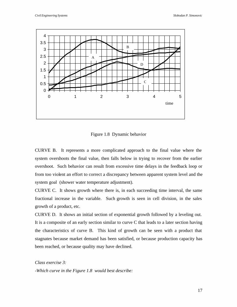
1.7 Complex System Behavior When positive and negative loops are combined, a variety of patterns are possible. Figure
1.8 illustrates four typical system behavior patters.
CURVE A. Typical feedback system in which variable rises at a decreasing rate toward a
final value (here a value of 3). The curve might represent information that gives the
apparent level of a system as understanding increases toward the true value. Or the curve
might represent the way the water is release from a reservoir into an irrigation canal. The
change toward the final value is more rapid at first and approaches more and more slowly
as the discrepancy decreases between present and final value.
Civil Engineering Systems Slobodan P. Simonovic
17
0
0.5
1
1.5
2
2.5
3
3.5
4
0 1 2 3 4 5
time
Figure 1.8 Dynamic behavior
CURVE B. It represents a more complicated approach to the final value where the
system overshoots the final value, then falls below in trying to recover from the earlier
overshoot. Such behavior can result from excessive time delays in the feedback loop or
from too violent an effort to correct a discrepancy between apparent system level and the
system goal (shower water temperature adjustment).
CURVE C. It shows growth where there is, in each succeeding time interval, the same
fractional increase in the variable. Such growth is seen in cell division, in the sales
growth of a product, etc.
CURVE D. It shows an initial section of exponential growth followed by a leveling out.
It is a composite of an early section similar to curve C that leads to a later section having
the characteristics of curve B. This kind of growth can be seen with a product that
stagnates because market demand has been satisfied, or because production capacity has
been reached, or because quality may have declined.
Class exercise 3:
-Which curve in the Figure 1.8 would best describe:
B
A
D
C
Civil Engineering Systems Slobodan P. Simonovic
18
1. How the temperature of a thermometer changes with time after it is immersed in a hot
liquid? __.
2. The position of a pendulum, which is displaced and allowed to swing, is best
described by curve __ .
3. Which curve describes the learning process? __
4. Industrialization: capital equipment used to produce more capital equipment. Which
curve describes the amount of capital equipment versus time? __
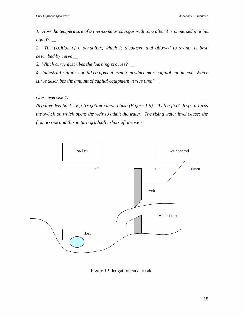
Class exercise 4:
Negative feedback loop-Irrigation canal intake (Figure 1.9): As the float drops it turns
the switch on which opens the weir to admit the water. The rising water level causes the
float to rise and this in turn gradually shuts off the weir.
Figure 1.9 Irrigation canal intake
switch
on off
weir control
up down
weir
water intake
float

Civil Engineering Systems Slobodan P. Simonovic
19
1. The water controls the water level which controls the weir opening, this is a __
system.
2. Sketch and label the flow diagram of the water intake system using symbols from the
feedback loop graph.
3. Modify the flow diagram by removing float and introducing manual control of the
weir.
4. The figure from question 3 shows an __ system.
5. FR is set at 0.1 m3/minute. In ten minutes there will be __ of water in the canal.
6. The units of measure must always accompany any numerical value to define the
quantity. The units of measure of water flow rate are __ / __ . The water volume is
measured in __ .
7. On the following figure, plot the water flow rate of 0.1 m3/minute.
8. If the FR = 0.04 m3/minute and if the canal is empty at time 0, the amount of water is
__ at 10 min
__ at 20 min
__ at 40 min
__ at 60 min.
9. Plot the amount of water in the canal for every point in time.
10. On the same graph, plot the water-time relationship showing the volume of water in
the canal for a flow rate of 0.2, 0.1 and 0.02 m3/min.
11. On the following graph use two vertical scales. Using the flow rate scale show
FR=0.05 m3/min. Using the volume scale show the volume of water ( m3 ) in the canal at
all points in time.
12. Using weir with float control (graph in problem 2) suppose that the flow rate is 0.2
m3/min when the canal is empty and declines proportionally to zero when the canal
contains 4 m3 .
13. Express FR as an equation.
14. Find T when W=0.
15. Replace T in the equation and find the FR when W=2.5m3. Check the value using the
graph from question 12.
Civil Engineering Systems Slobodan P. Simonovic
20
1.8 Creating Causal Loop Diagrams
To start drawing a causal loop diagram, decide which events are of interest in developing
a better understanding of system structure. From these events, move to showing (perhaps
only qualitatively) the pattern of behavior over time for the quantities of interest. Finally,
once the pattern of behavior is determined, use the concepts of positive and negative
feedback loops, with their associated generic patterns of behavior, to begin constructing a
causal loop diagram which will explain the observed pattern of behavior.
The following tutorial for drawing causal loop diagrams are based on guidelines by
Forester (1990) and Senge (1990)
1. Think of the elements in a causal loop diagram as variables which can go up or
down, but don't worry if you cannot readily think of existing measuring scales for these
variables.
• Use nouns or noun phrases to represent the elements, rather than verbs. That is,
the actions in a causal loop diagram are represented by the links (arrows), and not
by the elements.
• Be sure that the definition of an element makes it clear which direction is up for
the variable.
• Generally it is clearer if you use an element name for which the positive sense is
preferable.
• Causal links should imply a direction of causation, and not simply a time
sequence. That is, a positive link from element A to element B does not mean first
A occurs and then B occurs. Rather it means, when A increases then B increases.
2. As you construct links in your diagram, think about possible unexpected side effects
which might occur in addition to the in influences you are drawing. As you identify these,
decide whether links should be added to represent these side effects.
3. For negative feedback loops, there is a goal. It is usually clearer if this goal is explicitly
shown along with the gap that is driving the loop toward the goal. This is illustrated by
the examples in the preceding section on regulating room temperature.

Civil Engineering Systems Slobodan P. Simonovic
21
4. A difference between actual and perceived states of a process can often be important in
explaining patterns of behavior. Thus, it may be important to include causal loop
elements for both the actual value of a variable and the perceived value. In many cases,
there is a lag (delay) before the actual state is perceived. For example, when there is a
change in concrete quality, it usually takes a while before we perceive this change.
5. There are often differences between short term and long term consequences of actions,
and these may need to be distinguished with different loops.
6. If a link between two elements needs a lot of explaining, you probably need to add
intermediate elements between the two existing elements that will more clearly specify
what is happening.
7. Keep the diagram as simple as possible, subject to the earlier points. The purpose of
the diagram is not to describe every detail of the management process, but to show those
aspects of the feedback structure which lead to the observed pattern of behavior.
1.9 Problems
1.1 Fill in your answer:
A governor and the engine to which it is coupled form a __ to deliver power at
constant engine speed.
Thermostat is a __ system that reacts to the temperature that is being controlled.
The parts of a feedback system form a structure shaped as a (chain/loop) __.
The __ arrangement of a __ system brings the result of past actions back to guide
present decisions.
The information about the system changes as a result of past __ governing __ that
have changed the levels of the system of which we are a part.
1.2 Using a water level of 0.8 m3, what is the flow rate from equation FR=1/20 (2-
WL)?_ _
How much water will be added during the next four seconds? __
How much water is in the tank after the first 8 seconds? __
Using a table calculate flow rate and water level every 4 seconds. Complete the
table for 1 min and plot the curves of water level and flow rate as your calculation
Civil Engineering Systems Slobodan P. Simonovic
22
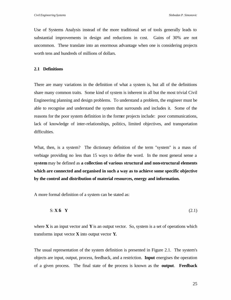
progresses (it is important for learning that you actually do these calculations and
the plotting-pay attention to the way in which the variables are changing and why).
1.3 Test are you a system thinker: A good systems thinker, particularly in an
organizational setting, is someone who can see four levels operating simultaneously:
events, patterns of behavior, systems and mental models.
Group exercises:
STEP 1 The problem is ...
(The issue should be important to you and your team. Purpose is to lay the groundwork
for a systems understanding of your own situation. Choose a chronic problem. Choose a
problem limited in scope. Choose a problem whose history is known, and which you can
describe. Make sure your description of the problem is as accurate as possible. Do not
jump to the conclusions. Be nonjudgemental.)
STEP 2. Telling the story. (This process is known as model building. During this phase,
you develop a theory or hypothesis that makes sense and could explain why the system is
generating the problems you see. Do not take classical problem solving, precisely
defining a problem statement. Try to keep in mind the following question: How did we
(through our processes and our practices) contribute to or create the circumstances
(good or bad) we face now?
Option A: Make the list. (Identify the key factors that seem likely to capture the problem
or are critical to telling the story)
Option B: Draw a picture. (Draw the most important graph about your problem and add
a few words.
The five WHYS. First why- pick the symptom where you wish to start. Write it down with
plenty of room around.
The successive whys. Repeat the process for every statement you wrote.
1.4 In question below (i) assign polarities to each of the arrows; (ii) assign polarities to
each of the feedback loops; (iii) write a brief but insightful paragraph describing the
role of the feedback loops in your diagram. [Don't describe every link in your diagram --
assume your figure and its polarities take care of that; talk mainly about the loops.]

Civil Engineering Systems Slobodan P. Simonovic
23
Feedback loops in highway construction and traffic density. After assigning polarities,
consider what the left-hand loop would do by itself? What do the right-hand loops
contribute?
1.5 Present a loop of your own (from your own thinking or from book of some sort).
Tell enough in words so that your picture and the story it tries to tell are clear.
1.10 References
Bruner, J.S., (1960), The process of education, Harward University Press, Harward,
USA..
Forester, J.W. (1990), Principles of systems, Productivity Press, Portland, Oregon, USA,
first publication in 1968.
Senge, P.M., (1990), Fifth discipline-The art and practice of the learning organization,
Doubleday, New York, USA.

Civil Engineering Systems Slobodan P. Simonovic
24
2. SYSTEMS ANALYSIS
Systems Analysis is the use of rigorous methods to help determine preferred plans and
designs for complex, often large-scale systems. It combines knowledge of the available
analytic tools, understanding of when each is more appropriate, and skill in applying them to
practical problems. It is both mathematical and intuitive, as is all planning and design (de
Neufville, 1990).
Systems Analysis is a relatively new field. Its development parallels that of the computer,
the computational power of which enables us to analyse complex relationships, involving
many variables, at reasonable cost. Most of its techniques depend on the use of the
computer for practical applications. Systems Analysis may be thought of as the set of
computer-based methods essential for the planning of major projects. It is thus central to a
modern engineering curriculum.
Systems Analysis covers much of the same material as operations research, in particular
linear and dynamic programming and decision analysis. The two fields differ substantially
in direction, however. Operations research tends to be interested in specific techniques and
their mathematical properties. Systems Analysis focuses on the use of the methods.
Systems Analysis includes the topics of engineering economy, but goes far beyond them in
depth of concept and scope of coverage. Now that both personal computers and efficient
financial calculators are available, there is little need for professionals to spend much time
on detailed calculations. It is more appropriate to understand the concepts and their
relationship to the range of techniques available to deal with complex problems.
Systems Analysis emphasises the kinds of real problems to be solved; considers the
relevant range of useful techniques, including many besides those of operations research;
and concentrates on the guidance they can provide toward improving plans and designs.
Civil Engineering Systems Slobodan P. Simonovic
25
Use of Systems Analysis instead of the more traditional set of tools generally leads to
substantial improvements in design and reductions in cost. Gains of 30% are not
uncommon. These translate into an enormous advantage when one is considering projects
worth tens and hundreds of millions of dollars.
2.1 Definitions
There are many variations in the definition of what a system is, but all of the definitions
share many common traits. Some kind of system is inherent in all but the most trivial Civil
Engineering planning and design problems. To understand a problem, the engineer must be
able to recognise and understand the system that surrounds and includes it. Some of the
reasons for the poor system definition in the former projects include: poor communications,
lack of knowledge of inter-relationships, politics, limited objectives, and transportation
difficulties.
What, then, is a system? The dictionary definition of the term "system" is a mass of
verbiage providing no less than 15 ways to define the word. In the most general sense a
system may be defined as a collection of various structural and non-structural elements
which are connected and organised in such a way as to achieve some specific objective
by the control and distribution of material resources, energy and information.
A more formal definition of a system can be stated as:
S: X → Y (2.1)
where X is an input vector and Y is an output vector. So, system is a set of operations which
transforms input vector X into output vector Y.
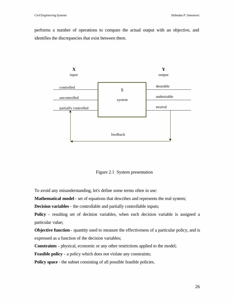
The usual representation of the system definition is presented in Figure 2.1. The system's
objects are input, output, process, feedback, and a restriction. Input energises the operation
of a given process. The final state of the process is known as the output. Feedback
Civil Engineering Systems Slobodan P. Simonovic
26
performs a number of operations to compare the actual output with an objective, and
identifies the discrepancies that exist between them.
To avoid any misunderstanding, let's define some terms often in use:
Mathematical model - set of equations that describes and represents the real system;
Decision variables - the controllable and partially controllable inputs;
Policy - resulting set of decision variables, when each decision variable is assigned a
particular value;
Objective function - quantity used to measure the effectiveness of a particular policy, and is
expressed as a function of the decision variables;
Constraints - physical, economic or any other restrictions applied to the model;
Feasible policy - a policy which does not violate any constraints;
Policy space - the subset consisting of all possible feasible policies.
Figure 2.1 System presentation
S
system
X input
Y output
desirable
undesirable
neutral
feedback
controlled
uncontrolled
partially controlled

Civil Engineering Systems Slobodan P. Simonovic
27
Class exercise 1:
You are charged with the design of the UWO parking lot Z. Specify in words possible
objectives, the unknown decision variables, and the constraints that must be met by any
solution of the problem.
2.2 Systems approach
The systems approach is a general problem-solving technique that brings more objectivity to
the planning/design processes. It is, in essence, good design; a logical and systematic
approach to problem solution in which assumptions, goals, objectives, and criteria are
clearly defined and specified. Emphasis is placed on relating system performance to these
goals. A hierarchy of systems, which allows handling of a complex system by looking at its
component parts or subsystems, is identified. Quantifiable and nonquantifiable aspects of
the problem are identified, and immediate and long-range implications of suggested
alternatives are evaluated.
The systems approach establishes the proper order of inquiry and helps in the selection of
the best course of action that will accomplish a prescribed goal by broadening the
information base of the decision maker; by providing a better understanding of the system
and the inter-relatedness of the system and its component subsystems; and by facilitating
the prediction of the consequences of several alternative courses of action.
The systems approach is a framework for analysis and decision making. It does not solve
problems, but does allow the decision maker to undertake resolution of a problem in a
logical, rational manner. While there is some art involved in the efficient application of the
systems approach, other factors play equally important roles. The magnitude and
complexity of decision processes require the most effective use possible of the scientific
(quantitative) methods of systems analysis. However, one has to be careful not to rely too
heavily on the methods of systems analysis. Outputs from simplified analyses have a
tendency to take on a false validity because of their complexity and technical elegance.

Civil Engineering Systems Slobodan P. Simonovic
28
The steps in the systems approach include (Jewell, 1986):
- Definition of the problem;
- Gathering of data;
- Development of criteria for evaluating alternatives;
- Formulation of alternatives;
- Evaluation of alternatives;
- Choosing the best alternative; and
- Final design/plan implementation.
Often several steps in the systems approach are considered simultaneously, facilitating
feedback and allowing a natural progression in the problem-solving process. The systems
approach has several defining characteristics. It is a repetitive process, with feedback
allowed from any step to any previous step. Without this feedback ability, the systems
approach is not being applied. Frequently, because systems analysis takes such a broad
approach to problem solving, interdisciplinary teams must be called in. Coordination and
commonality of technique among the disciplines is sometimes hard to achieve. However, if
applied with ingenuity and flexibility, the systems approach can provide a common basis for
understanding among specialists from seemingly unrelated fields and disciplines. Close
communication among the parties involved in applying the systems approach is essential if
this understanding is to be achieved.
Definition of the problem. Problem definition may require iteration and careful
investigation, because problem symptoms may mask the true cause of the problem. A key
step of problem definition requires the identification of any systems and subsystems that are
part of the problem, or related in some way to it. This set of systems and interrelationships
is called the environment of the problem. This environment sets the limit on factors that will
be considered when analysing the problem. Any factors that cannot be included in the
problem environment must be included as inputs to, or outputs from, the problem
environment.
Civil Engineering Systems Slobodan P. Simonovic
29
When defining the problem and its environment, the best approach is to make the definition
as general as possible. The largest problem over which there is a reasonable chance of
maintaining control should be the problem defined.
Gathering of Data. Gathering of data to assist in planning and design decision making
through the systems approach will generally be done in conjunction with several steps.
Some background data will have to be gathered at the problem definition stage and data
gathering and analysis will continue through the final plan/design and implementation stage.
Data that are gathered as the approach continues will help to identify when feedback to a
previous step is required.
Data will be required at the problem definition stage to evaluate if a problem really exists;
to establish what components, subsystems, and elements can be reasonably included in the
delineation of the problem environment; and to define interactions between components
and subsystems. Data will be needed during later steps to establish constraints on the
problem and systems involved in it, to increase the set of quantifiable variables and
parameters (constants) through statistical observation or development of measuring
techniques, to suggest what mathematical models might contribute effectively to the
analysis, to estimate values for coefficients and parameters used in any mathematical models
of the system, and to check the validity of any estimated system outputs. When feedback is
required, the data previously acquired can assist in redefining the problem, systems, or
system models.
Development of evaluative criteria. Evaluative criteria must be developed to measure the
degree of attainment of system objectives. These evaluative criteria will facilitate a rational
choice of a particular set of actions (from among a large number of feasible alternatives)
which will best accomplish the established objectives. Some evaluative criteria will provide
an absolute value of how good the solution is, such as the cost of producing one unit of
some product. Other evaluative criteria will only produce relative values that can be
compared among the alternatives to rank them in order of preference, as in economic
comparisons such as benefit/cost analysis.

Civil Engineering Systems Slobodan P. Simonovic
30
In most complex real world problems, more than one objective can be identified. A
quantitative or qualitative analysis of the trade-offs between the objectives must be made. It
may be possible to specify all but one objective as set levels of performance, which become
system constraints. Then the system can be designed to perform optimally in terms of the
remaining objective. For many problems, cost effectiveness would be the primary objective.
Cost effectiveness can be defined as the lowest possible cost for a set level of control of a
system, or the highest level of system control for a set cost.
Formulation of alternatives. Formulation of alternatives is essentially the development of
system models that, in conjunction with evaluative criteria, will be used in later analysis and
decision making. If at all possible, these models should be mathematical in nature.
However, it should not be assumed that mathematical model building and optimisation
techniques are either required or sufficient for application of the systems approach. Many
problems contain unquantifiable variables and parameters which would render results
generated by even the most elegant mathematical model meaningless. If it is not practical to
develop mathematical models, subjective models that describe the problem environment and
systems included can be constructed. Models allow a more explicit description of the
problem and its systems and facilitate the rapid examination of alternatives. The primary
emphasis in this text will be on problems that can at least partially be represented by
mathematical models. However, limitations of these models and appropriate applications of
subjective models will be indicated.
Effective model building is a combination of art and science. The science includes the
technical principles of mathematics, physics, and engineering science. The art is the
creative application of these principles to describe physical or social phenomena. Practice is
the best way to learn the art of model building, but this practice must be predicated on a
thorough understanding of the science. Although the art of modelling cannot be taught in a
single course, a course that introduces the student to the systems approach will lay the
foundation for further development.

Civil Engineering Systems Slobodan P. Simonovic
31
Evaluation of alternatives. To evaluate the alternatives that have been developed, some
form of analysis procedure must be used. Numerous mathematical techniques are available,
including the simplex method for linear programming models, the various methods for
solving ordinary and partial differential equations or systems of differential equations,
matrix algebra, various economic analyses, and deterministic or stochastic computer
simulation. Subjective analysis techniques may be used for multiobjective analysis, or
subjective analysis of intangibles.
The appropriate analysis procedures for a particular problem will generate a set of solutions
for the alternatives that can be tested according to the established evaluative criteria. In
addition, these solution procedures should allow efficient utilisation of manpower and
computational resources.
As part of the analysis stage, the importance of each variable should be checked. This is
called sensitivity analysis, and it involves testing how much the model output will change
for given changes in the values of the decision variable and model parameters.
Choosing the best alternative. Choice of the best alternative from among those analysed
must be made in the context of the objectives and evaluative criteria previously established,
but also must take into account nonquantifiable aspects of the problem such as aesthetic and
political considerations. The chosen alternative will greatly influence the development of
the final plan/design and will determine in large part the implementability of the suggested
solution.
Preferably the best alternative can be chosen from the mathematical optimisation within
feasibility constraints. Frequently, however, a system cannot be completely optimised.
Near optimum solutions can still be useful, especially if sensitivity analysis has shown that
the solution (and thus the objective function) is not sensitive to changes in the decision
variables near the optimum point.

Civil Engineering Systems Slobodan P. Simonovic
32
Final plan/design implementation. Actual final planning/design is primarily a technical
matter that is conducted within the constraints and specifications developed in earlier stages
of the systems approach. One of the end products of final planning or design is a report
which describes the recommendations made. To be effective, this report must also include
information on what has gone into the application of the systems approach to the problem.
The report should be written in the context of the audience for which it is intended. A well-
written nontechnical report can go a long way toward developing public support for the
recommended problem solution, whereas, a well-written technical report given the same
audience may be intimidating and actually reduce support for the recommendations.
2.3 Systems engineering
Systems engineering may be defined as the art and science of selecting from a large number
of feasible alternatives, involving substantial engineering content, that particular set of
actions which will best accomplish the overall objectives of the decision makers, within the
constraints of law, morality, economics, resources, politics, social life, nature, physics etc.
Another definition expresses the systems engineering as a set of methodologies for studying
and analysing the various aspects of a system (structural and non-structural) and its
environment by using mathematical and/or physical models.
Systems engineering is currently the popular name for the engineering processes of planning
and design used in the creating of a `system' or project of considerable complexity.
Design. The design of a system represents a decision about how resources should be
transformed to achieve some objectives. The final design is a choice of a particular
combination of resources and a way to use them; it is selected from other combinations
that would accomplish the same objectives. For example, the design of a building to
provide 100 apartments represents a selection of the number of floors, the spacing of the
columns, the type of materials used, and so on; the same result could be achieved in many
different ways.

Civil Engineering Systems Slobodan P. Simonovic
33
A design must satisfy a number of technical considerations. It must conform to the laws of
the natural sciences; only some things are possib le. To continue with the example of the
building, there are limits to the available strength of either steel or concrete, and this
constrains what can be built. The creation of a good design for a system thus requires solid
technical competence in the matter at hand. Engineers may take this fact to be self-evident,
but it often needs to be stressed to industrial or political leaders motivated by their hopes for
what a proposed system might accomplish.
Economics and values must also be taken into account in the choice of design; the best
design cannot be determined by technical considerations alone. Moreover, these issues tend
to dominate the final choice between many possible designs, each of which appears equally
effective technically. The selection of a design is then determined by the costs and relative
values associated with the different possibilities. The choice between constructing a
building of steel or concrete is generally a question of cost, as both can be essentially
equivalent technically. For more complex systems, political or other values may be more
important than costs. In planning an airport for a city for instance, it is usually the case that
several sites can be made to perform technically; the final choice hinges on societal
decisions about the relative importance of ease of access and the environmental impacts of
the airport, in addition to its cost.
Planning. Planning and design are so closely related that it is difficult to separate one from
the other. The planning process closely follows the systems approach, and may involve the
use of sophisticated analysis and computer tools. However, the scope of problems
addressed by planning is different from the scope of design problems. Basically, planning
is the formulation of goals and objectives that are consistent with political, social,
environmental, economic, technological, and aesthetic constraints; and the general
definition of procedures designed to meet those goals and objectives. Goals are the
desirable end states that are sought. They may be influenced by actions or desires of
government bodies, such as legislatures or courts; of special interest groups; or of
administrators. Goals may change as the interests of the concerned groups change.
Civil Engineering Systems Slobodan P. Simonovic
34
Objectives relate ways in which the goals can be reached. Planning should be involved in
all aspects of an engineering project, including preliminary investigations, feasibility studies,
detailed analysis and specifications for implementation and/or construction, and monitoring
and maintenance. A good plan will bring together diverse ideas, forces, or factors, and
combine them into a coherent, consistent structure that when implemented, will improve
target conditions without deprecating non-target conditions. Effective use of the systems
approach will help ensure that planning studies address the true problem at hand. Planning
studies that do not do this could not, if implemented, produce useful and desirable changes.
2.4 Mathematical modelling
In general, to obtain a way to control or manage a physical system we use a mathematical
model which closely represents the physical system. Then the mathematical model is solved
and its solution is applied to the physical system. Models, or idealised representations, are
an integral part of everyday life. Common examples of models include model aeroplanes,
portraits, globes, and so on. Similarly, models play an important role in science and
business, as illustrated by models of the atom, models of genetic structure, mathematical
equations describing physical laws of motion or chemical reactions, graphs, organisation
charts, and industrial accounting systems. Such models are invaluable for abstracting the
essence of the subject of inquiry, showing inter-relationships, and facilitating analysis
(Hillier and Lieberman, 1990).
Mathematical models are also idealised representations, but they are expressed in terms of
mathematical symbols and expressions. Such laws of physics as F = ma and E = mc2 are
familiar examples. Similarly, the mathematical model of a business problem is the system
of equations and related mathematical expressions that describe the essence of the problem.
Thus, if there are n related quantifiable decisions to be made, they are represented as
decision variables (say, x1, x2, ..., xn) whose respective values are to be determined. The
appropriate measure of performance (e.g. profit) is then expressed as a mathematical
function of these decision variables (e.g. P = 3x1 + 2x2 + ... + 5xn). This function is called
the objective function. Any restrictions on the values that can be assigned to these decision

Civil Engineering Systems Slobodan P. Simonovic
35
variables are also expressed mathematically, typically by means of inequalities or equations
(e.g. x1 + 3x1x2 + 2x2 ≤ 10). Such mathematical expressions for the restrictions often are
called constraints. The constants (coefficients or right-hand sides) in the constraints and
the objective function are called the parameters of the model. The mathematical model
might then say that the problem is to choose the values of the decision variables so as to
maximise the objective function, subject to the specified constraints. Such a model, and
minor variations of it, typify the models used in operations research.
Mathematical models have many advantages over a verbal description of the problem. One
obvious advantage is that a mathematical model describes a problem much more concisely.
This tends to make the overall structure of the problem more comprehensible, and it helps to
reveal important cause-and-effect relationships. In this way, it indicates more clearly what
additional data are relevant to the analysis. It also facilitates dealing with the problem in its
entirety and considering all its inter-relationships simultaneously. Finally, a mathematical
model forms a bridge to the use of high-powered mathematical techniques and computers to
analyse the problem. Indeed, packaged software for both microcomputers and mainframe
computers is becoming widely available for many mathematical models.
The procedure of selecting the set of decision variables which maximises/ minimises the
objective function subject to the systems constraints, is called the optimisation procedure .
The following is a general optimisation problem. Select the set of decision variables x*1, x*
2,
... , x*n such that
Min or Max f(x1, x2, ..., xn)
subject to:
g1 (x1, x2, ..., xn) ≤ b1
g2 (x1, x2, ..., xn) ≤ b2 (2.2)
gm (x1, x2, ..., xn) ≤ bm

Civil Engineering Systems Slobodan P. Simonovic
36
where b1, b2, ..., bm are known values.
If we use the matrix notation (2.2) can be rewritten as:
Min or Max f (x) (2.3)
subject to:
gj (x) ≤ bj j = 1, 2, ..., m
When optimisation fails, due to system complexity or computational difficulty, a reasonable
attempt at a solution may often be obtained by simulation. Apart from facilitating trial and
error design, simulation is a valuable technique for studying the sensitivity of system
performance to changes in design parameters or operating procedure. Simulation will be
presented in the Section 3 of this text.
According to equations (2.2) and (2.3) our main goal is the search for an optimal, or best
solution. Some of the techniques developed for finding such solutions are presented in
Sections 4 and 5 of this text. However, it needs to be recognised that these solutions are
optimal only with respect to the model being used. Since the model necessarily is an
idealised rather than an exact representation of the real problem, there cannot be any
Utopian guarantee that the optimal solution for the model will prove to be the best possible
solution that could have been implemented for the real problem. There just are too many
imponderables and uncertainties associated with real problems. However, if the model is
well formulated and tested, the resulting solution should tend to be a good approximation to
the ideal course of action for the real problem. Therefore, rather than be deluded into
demanding the impossible, the test of the practical success of an operations research study
should be whether it provides a better guide for action than can be obtained by other means.
Civil Engineering Systems Slobodan P. Simonovic
37
The eminent management scientist and Nobel Laureate in Economics, Herbert Simon,
points out that satisficing is much more prevalent than optimising in actual practice. In
coining the term satisficing as a combination of the words satisfactory and optimising,
Simon is describing the tendency of managers to seek a solution that is "good enough" for
the problem at hand. Rather than trying to develop various desirable objectives (including
well-established criteria for judging the performance of different segments of the
organisation), a more pragmatic approach may be used. Goals may be set to establish
minimum satisfactory levels of performance in various areas, based perhaps on past levels
of performance or on what the competition is achieving. If a solution is found that enables
all of these goals to be met, it is likely to be adopted without further ado. Such is the nature
of satisficing.
The distinction between optimising and satisficing reflects the difference between theory
and the realities frequently faced in trying to implement that theory in practice. In the words
of Samuel Eilon, "optimising is the science of the ultimate; satisficing is the art of the
feasible."
2.5 Classification of mathematical models and optimisation techniques
Depending on the nature of the objective function and the constraints, the optimisation
problem can be classified as:
Linear - the objective function and all the constraints are linear in terms of the decision
variables;
Nonlinear - part or all of the constraints and/or the OF are nonlinear;
Deterministic - if each variable and parameter can be assigned a definite fixed number or a
series of fixed numbers for any given set of conditions;
Probabilistic/Stochastic - contain variables the value of which are subject to some measure
of randomness or uncertainty;
Static - models which do not explicitly take time into account;
Dynamic - models which involve time-dependent interactions;

Civil Engineering Systems Slobodan P. Simonovic
38
Distributed Parameters - models which take into account detailed variations in behaviour
from point to point throughout the system;
Lumped Parameters - models which ignore the variations and the parameters and
dependent variables can be considered to be homogeneous throughout the entire system.
Several techniques of optimisation are available to solve the above optimisation problems,
such as:
· calculus;
· linear programming;
· non- linear programming;
- direct search;
- gradient search;
- complex method;
- geometric programming; and
- other.
· dynamic programming;
· others.
For dynamic systems:
· queuing theory;
· game theory;
· network theory;
· the calculus of variation;
· the maximum principle;
· quasi-linearisation; and
· others.
All the models and techniques mentioned up to now are dealing with the single objective
function (Eqns. 2.2 and 2.3). If we have problems which require more than one objective
functions then in mathematical terms we are dealing with "vector optimisation" or
multiobjective optimisation presented in Section 6 of this manuscript.

Civil Engineering Systems Slobodan P. Simonovic
39
Class exercise 2
Choose the optimization technique for solving the problem from the Exercise 1 according to
the classification above. Discuss the characteristics of the parking lot design problem from
the model classification point of view.
Class exercise 3:
Tables 2.1, 2.2, and 2.3 provide possible recommendations of model choice for different
steps of the water resources planning procedure (Simonovic 1989).
2.6 Problems
2.1 What are the characteristics of civil engineering planning or management problems
that are most suitable for analysis using quantitative systems analysis techniques?
2.2 Identify one engineering planning problem and specify in words possible objectives,
the unknown decision variables whose values need to be determined, and the constraints
or relationships that must be met by any solution of the problem.
2.3 Describe the political, economic, technical, aesthetic, etc. issues involved in one civil
engineering problem you are familiar with.
2.4 In the above defined problem (2.2) separate the quantitative variables from
nonquantitative. Identify the decision variables in both sets. Identify the objectives, both
quantitative and nonquantitative. Of the quantitative objectives, indicate the indices of
quantification which most appropriately reflect that objective. Also, indicate those which
might be reduced to common terms (e.g., dollars). Identify all possible constraints. Using
the classifications presented in class identify appropriate solution techniques for your
problem.
2.5 In most general terms, list all the stages of civil engineering planning and describe
the task of each.
Civil Engineering Systems Slobodan P. Simonovic
40
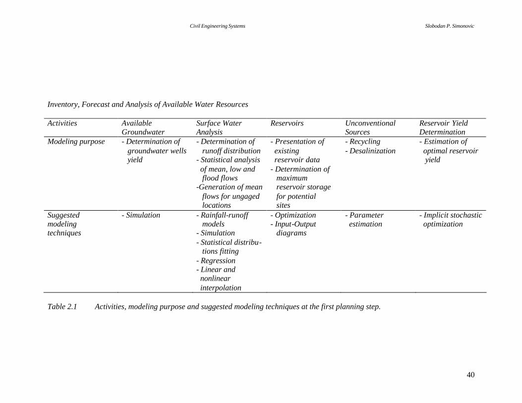
Inventory, Forecast and Analysis of Available Water Resources Activities Available
Groundwater Surface Water Analysis
Reservoirs Unconventional Sources
Reservoir Yield Determination
Modeling purpose - Determination of groundwater wells yield
- Determination of runoff distribution - Statistical analysis of mean, low and flood flows -Generation of mean flows for ungaged locations
- Presentation of existing reservoir data - Determination of maximum reservoir storage for potential sites
- Recycling - Desalinization
- Estimation of optimal reservoir yield
Suggested modeling techniques
- Simulation - Rainfall-runoff models - Simulation - Statistical distribu- tions fitting - Regression - Linear and nonlinear interpolation
- Optimization - Input-Output diagrams
- Parameter estimation
- Implicit stochastic optimization
Table 2.1 Activities, modeling purpose and suggested modeling techniques at the first planning step.

Civil Engineering Systems Slobodan P. Simonovic
41
Inventory, Forecast and Analysis of Water Demand Activities Municipal and
Industrial Water Supply
Irrigation Power Production Water Quality Control
Other Uses
Modeling Purpose
-Estimation of population growth - Prediction of industrial development
-Estimation of the water demand - Derivation of crop yield-soil moisture relation
- Estimation of power demand - Thermal and hydro power production
- Estimation of clean water amount necessary for dilution
- Recreation requirements -Fish production - Wildlife
Suggested modeling techniques
-Systems dynamics model (diagram of flows, of people, of resources, and products) -Input-output diagrams -Trends estimation
- Simulation - Mathematical formula (Blaney Criddle) - Optimization of water allocation (stochastic dynamic programming) - Optimization of crop structure (linear programming)
- Input-output modeling - Simulation - Optimization - Interpretive structural modeling
- Quality simulation - Optimization of wastewater discharge sites - Optimization of waste load
- Water Level computation (simulation) - Water quality simulation
Table 2.2 Activities, modeling purpose and suggested modeling techniques at the second planning step.

Civil Engineering Systems Slobodan P. Simonovic
42
Comparison and Ranking the Alternative Solutions Activities Setting objectives and
developing evaluation criteria
Evaluating the alternatives
Selecting an alternative
Sensitivity analysis
Modeling purpose - Model of purposes for every “water system”
- Evaluation of alternative sets according to all used criteria
- Decision making models for ranking alternatives
- Analyzing the influence of decision makers’ preferences and model parameters on alternatives rank
Suggested modeling Techniques
- Objectives tree - Hierarchical diagram - Interaction matrices
- Cost estimation model - Cost-benefit model - Cost-effectiveness model
- Discrete multi- objective techniques - Decision table (showing ranking of alternatives for each criteria) - Criterion function (mathematical expression for establishing the overall ranking of alternative)
- Preference relations - Discrete multi- objective techniques
Table 2.3 Activities, modeling purpose and suggested modeling techniques at the fourth planning step

Civil Engineering Systems Slobodan P. Simonovic
43
2.7 References
De Neufville, R., (1990), Applied Systems Analysis: Engineering Planning and
Technology Management, McGraw Hill, New York, USA.
Hillier, F.S. and G.J. Lieberman, (1990), Introduction to Mathematical Programming,
McGraw Hill, New York, USA.
Jewell, T.K., (1986), A Systems Approach to Civil Engineering Planning and Design,
Harper and Row, New York, USA.
Simonovic, S.P., (1989), “Application of Water Resources Systems Concept to the
Formulation of a Water Master Plan”, Water International, 14, 37-50.
Civil Engineering Systems Slobodan P. Simonovic
44
3. SYSTEM SIMULATION
3.1 Introduction
Simulation models “describe” how a system operates, and are used to determine changes
resulting from a specific course of action. Such models are sometimes referred to as
“cause-and-effect” models. They describe the state of the system in response to various
inputs but give no direct measure of what decisions should be taken to improve the
performance of the system. Therefore, the simulation is problem solving technique
which contains the following phases :
a) development of a model of the system;
b) operation of the model (i.e. generation of outputs resulting from the application of
inputs); and
c) observation and interpretation of the resulting outputs.
The essence of simulation is modeling and experimentation. Simulation does not directly
produce “the answer” to a given problem. In the graphical form simulation procedure is
represented in Figure 3.1. Simulation includes a wide variety of procedures. In order to
choose among, and use them effectively, the potential user must know:
i) how they operate;
ii) how they can be expected to perform; and
iii) how this performance relates to the problem under investigation.
Major components of a simulation model are :
Input : quantities that “drive” the model (in water resources engineering models
for example a principal input is the set of streamflows, rainfall sequences,
pollution loads, water and power demands, etc.).
Physical Relationships : mathematical expression of the relationship among the physical
variables of the system being modeled (continuity, energy conservation
reservoir volume and elevation, outflow relations, routing equations, etc.).

Civil Engineering Systems Slobodan P. Simonovic
45
Figure 3.1 The simulation procedure
Nonphysical Relationships : those that define economic variables, political conflicts,
public awareness, etc.
Operation Rules : the rules that govern operational control.
Outputs : the final product of operations on inputs by the physical and nonphysical
relations in accordance with operating rules.
Start
decomposition of system
computer programming
model verification
operation of the model
analysis of the resulting outputs
alternative inputs
STOP

Civil Engineering Systems Slobodan P. Simonovic
46
Engineering domain can benefit from already available computer-based simulation
modeling tools. There are numerous tools used for implementing simulation in Civil
Engineering planning and design. Complex Civil Engineering problems heavily rely on
systems thinking, which is defined as the ability to generate understanding through
engaging in the mental model-based processes of construction, comparison, and
resolution. Computer software tools like STELLA, DYNAMO, VENSIM, POWERSIM
(High Performance Systems, 1992; Lyneis et al., 1994; Ventana, 1996; Powersim Corp.,
1996) and others help the execution of these processes. One that will be used in this
course is Vensim environment developed to support a special simulation approach known
as System Dynamics.
3.2 System Dynamics simulation approach for Civil Engineering problems
System Dynamics simulation approach relies on understanding complex inter-
relationships existing between different elements within a system. This is achieved by
developing a model that can simulate and quantify the behavior of the system. Simulation
of the model over time is considered essential to understand the dynamics of the system.
Understanding of the system and its boundaries, identifying the key variables,
representation of the physical processes or variables through mathematical relationships,
mapping the structure of the model and simulating the model for understanding its
behavior are some of the major steps that are carried out in the development of a system
dynamics simulation model. It is interesting to note that the central building blocks of the
principles of system dynamics approach are well suited for modeling any physical
system.
System dynamics simulation tools are well suited for representing mental models that have
been developed using systems thinking paradigm introduced in Section 1 of this text.
Practically, these tools are built around a progression of structures. Stocks, flows, converters
and connectors are the principal building blocks of structure and they are discussed in details
later in this section.

Civil Engineering Systems Slobodan P. Simonovic
47
The power and simplicity of use of system dynamics simulation applications is not
comparable with those developed in functional algorithmic languages. In a very short
period of time, the users of the simulation models developed by system dynamics tools
can experience the main advantages of this approach. The power of simulation is the ease
of constructing “what if” scenarios and tackling big, messy, real-world problems. In
addition, general principles upon which the system dynamics simulation tools are
developed apply equally to social, natural, and physical systems. Using these tools in
Civil Engineering allows enhancement of models by adding social, economic, and
ecological sectors into the model structure.
System dynamics is an academic discipline introduced in the 1960s by the researchers at
the Massachusetts Institute of Technology. System dynamics was originally rooted in the
management and engineering sciences but has gradually developed into a tool useful in
the analysis of social, economic, physical, chemical, biological and ecological systems
(Sterman, 2000). In the field of system dynamics, a system is defined as a collection of
elements which continually interact over time to form a unified whole. The underlying
pattern of interactions between the elements of a system is called the structure of the
system. One familiar water resources engineering example of a system is a reservoir. The
structure of a reservoir is defined by the interactions between inflow, storage, outflow,
and other variables specific to a particular reservoir location (storage curve, evaporation,
infiltration, etc.). The structure of the reservoir includes the variables important in
influencing the system. The term dynamics refers to change over time. If something is
dynamic, it is constantly changing in response to the stimuli influencing it. A dynamic
system is thus a system in which the variables interact to stimulate changes over time.
System Dynamics is a methodology used to understand how systems change over time.
The way in which the elements or variables composing a system vary over time is
referred to as the behavior of the system. In the reservoir example, the behavior is
described by the dynamics of reservoir storage growth and decline. This behavior is due
to the influences of inflow, outflow, losses and environment, which are elements of the
system. One feature which is common to all systems is that a system’s structure
determines the system’s behavior. System Dynamics links the behavior of a system to its

Civil Engineering Systems Slobodan P. Simonovic
48
underlying structure. System Dynamics can be used to analyze how the structure of a
physical, biological, or any other system can lead to the behavior which the system
exhibits. By defining the structure of a reservoir, it is possible to use system dynamics
analysis to trace out the behavior over time of the reservoir based upon its structure.
The structure-behavior link need not be limited to systems which are well defined
historically or analytically. System Dynamics can also be used to analyze how structural
changes in one part of a system might affect the behavior of the system as a whole.
Perturbing a system allows one to test how the system will respond under varying sets of
conditions. Once again referring to a reservoir, someone can test the impact of a drought
on the reservoir or analyze the impact of the elimination of a particular user on the
behavior of the entire system.
In addition to relating system structure to system behavior and providing users a tool for
testing the sensitivity of a system to structural changes, System Dynamics requires a
person to partake in the rigorous process of modeling system structure. Modeling a
system structure forces a user to consider details typically glossed over within a mental
model.
3.3 Basic Building Blocks of System Dynamics Simulation Environments
The stock and flow notation provides a general way to graphically characterize any
system process. This may seem ambitious: any process! However, if we consider the
characteristics that are generally shared by all engineering processes and the components
which make up these processes, it is a remarkable fact that all such processes can be
characterized in terms of variables of two types, stocks (levels, accumulations) and flows
(rates).
The basic parts of Vensim language are: Stocks (Box Variable; Level), Rates (Flows),
Auxiliary Variables and Arrows (Connectors). They have a very particular meaning and
full understanding of it is essential for accurate System dynamics simulation modeling.

Civil Engineering Systems Slobodan P. Simonovic
49
Levels
Levels or stocks are the nouns of the Vensim language. Looking at the magnitudes of the
stocks at a point in time will tell you how things “are” within a system at that point in
time.
Stocks are signified by rectangles. Operationally, stocks function as accumulators.
Think about it…accumulations are everywhere! The food in your stomach. The money
in your wallet. The knowledge in your head. The love in your heart. All are
accumulations. Stocks can be used to depict both material and non-material
accumulations.
The magnitudes of Stocks within a system persist even if the magnitudes of all the
activities fall to zero. When you take a snapshot of a system only the accumulations that
the activities had filled and drained would appear in the picture. The picture would show
the state of the system at that point in time.
Because they accumulate, stocks often act as “buffers” within a system. In this role,
stocks enable inflows and outflows to be out of balance with each other – i.e., out of
equilibrium. For example, it was stocks which enabled us to move beyond the hunter and
gatherer phase of our existence! If we had not figured out how to store food, we’d still be
spending all of our time looking for food because we have to eat what we killed or found,
right when we killed or found it. By accumulating inventories of food, we could
consumer calories when we wanted, and the rate at which we consumed them could at
times be far in excess of the rate at which we were adding food to the inventory.
Rates
Levels and rates (stocks and flows) fit together. If stocks are nouns, flows are verbs.
You don’t have one without the other. If there is an accumulations of something, that
accumulation had to result from some activity, a flow of something. And if there is a
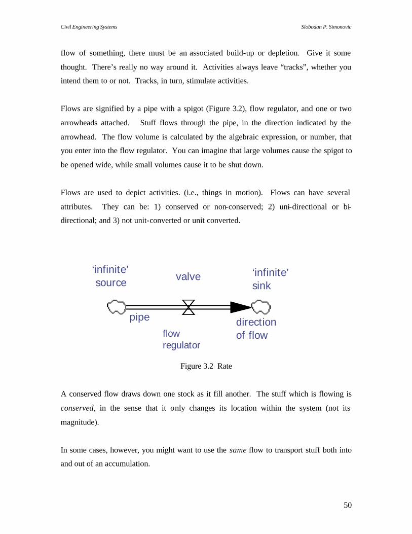
Civil Engineering Systems Slobodan P. Simonovic
50
flow of something, there must be an associated build-up or depletion. Give it some
thought. There’s really no way around it. Activities always leave “tracks”, whether you
intend them to or not. Tracks, in turn, stimulate activities.
Flows are signified by a pipe with a spigot (Figure 3.2), flow regulator, and one or two
arrowheads attached. Stuff flows through the pipe, in the direction indicated by the
arrowhead. The flow volume is calculated by the algebraic expression, or number, that
you enter into the flow regulator. You can imagine that large volumes cause the spigot to
be opened wide, while small volumes cause it to be shut down.
Flows are used to depict activities. (i.e., things in motion). Flows can have several
attributes. They can be: 1) conserved or non-conserved; 2) uni-directional or bi-
directional; and 3) not unit-converted or unit converted.
Figure 3.2 Rate
A conserved flow draws down one stock as it fill another. The stuff which is flowing is
conserved, in the sense that it only changes its location within the system (not its
magnitude).
In some cases, however, you might want to use the same flow to transport stuff both into
and out of an accumulation.
‘infinite’ source valve ‘infinite’
sink
pipe
flow regulator
direction of flow
Civil Engineering Systems Slobodan P. Simonovic
51
In most cases, flows are dominated in the same units of “stuff” as the stocks to which
they are attached. For example, bathtubs hold water. You would not expect to have jello,
motor oil or pasta flowing through the faucet or the drain. The stock would be
denominated in units of water. The flow also would be denominated in units of water,
with the suffix per time. When the units are not converted, the only difference between
stock and flow denomination in the “per time” suffix.
So, stocks and flows are inseparable. You can’t have one without the other. Both are
necessary for generating change over time, or dynamics. If we want only a static
snapshot of reality, stocks alone would be sufficient. But without flows, no change in the
magnitude of the stocks could occur. In order to move from snapshots to movies, we
need flows.
Fortunately for us, stocks and flows do exist in combination. When stocks de-couple
rates of flow, they serve as buffers, or shock-absorbers. Because stocks play this role, we
do not need to match inflows to outflows all the time.
Auxiliary variables
Auxiliary variables often function as adverbs, modifying the activities (or verbs) within
the system. But they also serve many other functions, and so are really best characterized
as “catchalls”. Auxiliary variables transform inputs into outputs. They can represent
either information or material quantities. They often are used to break out the detail of
the logic which otherwise would be buried within a flow regulator. Frequently they
represent “score-keeping” variables such as cost, cycle-time, profit, etc. Unlike levels,
auxiliary variables do not accumulate. The value for an auxiliary variable is re-calculated
from scratch in each time step. Auxiliary variables thus have no “memory”. Auxiliary
variables will play one of four roles: stock-related, flow-related, stock/flow related, and
external input-related.
In their stock-related role, auxiliary variables can provide an alternate way to measure the
magnitude of a stock, or they sometimes can be used to substitute for a stock concept.

Civil Engineering Systems Slobodan P. Simonovic
52
Auxiliary variables can also play flow-related roles in the models. The roles are twofold.
First, they can be used to “roll up” the net of several flow processes. Or, they can be used
to break out the components of the logic of a flow, so as to avoid diagram clutter.
The final category of use for auxiliary variables is “external inputs”. External inputs
include some time series inputs (often implemented via the graphical function), as well as
various built- in functions.
Arrows
The final building block is the arrow. Arrows link stocks to auxiliary variables, stocks to
flow regulators, flow regulators to flow regulators, auxiliary variables to flow regulators,
and auxiliary variables to other auxiliary variables. Arrows represent inputs and outputs,
not inflows and outflows! Arrows do not take on numerical values-they merely transmit
values taken on by other building blocks. When you step on a scale and look down at
your weight as registered on the dial, the resulting numerical magnitude is transmitted to
your eye without having any influence whatsoever on the numerical value. Such
transmissions would be represented using an arrow. Arrows cannot connect into a stock!
Only flows can change stocks.
3.4 System Dynamics Modeling Process
Though there is no universally accepted process for developing and using good quality
system dynamics models there are some basic practices that are quite commonly used.
The following steps are a useful guideline.
Issue statement. The issue statement is simply a statement of the problem that makes it
clear what the purpose of the model will be. Clarity of purpose is essential to effective
model development. Developing a model of a system or process without specifying how
the system needs to be improved or what specific behavior is problematic is difficult.
Having a clear problem in mind makes it easier to develop models with good practical
applicability.

Civil Engineering Systems Slobodan P. Simonovic
53
Variable Identification. Identify some key quantities that will need to be included in the
model for the model to be able to address the issues at hand. Usually a number of these
are very obvious. It can sometimes be useful just to write down all of the variables that
might be important and try to rank them in order to identify the most important ones.
Reference modes. A reference mode is a pattern of behavior over time. Reference
modes are drawn as graphs over time for key variables, but are not necessarily graphs of
observed behavior. Rather, reference modes are cartoons that show a particular
characteristic of behavior that is interesting. For example, a company's sales history may
be growing but bumpy, and the reference mode may be the up and down movement
around the growth trend. Reference modes can refer to past behavior, or future behavior.
They can represent what you expect to have happen, what you fear will happen and what
you hope will happen. Reference modes should be drawn with an explicitly labeled time
axis to help refine, clarify and bound a problem statement.
Reality Check. Define some Reality Check statements about how things must
interrelate. These include a basic understanding of what actors are involved and how
they interact, along with the consequences for some variables of significant changes in
other variables. Reality Check information is often simply recorded as notes (often
mental notes) about what connections need to exist. It is based on knowledge of the
system being modeled.
Dynamic hypotheses. A dynamic hypothesis is a theory about what structure exists that
generates the reference modes. A dynamics hypothesis can be stated verbally, as a causal
loop diagram, or as a stock and flow diagram. The dynamic hypotheses you generate can
be used to determine what will be kept in models, and what will be excluded. Like all
hypotheses, dynamic hypotheses are not always right. Refinement and revision is an
important part of developing good models.
Civil Engineering Systems Slobodan P. Simonovic
54
Simulation Model. A simulation model is the refinement and closure of a set of
dynamic hypotheses to an explicit set of mathematical relationships. Simulation models
generate behavior through simulation. A simulation model provides a laboratory in
which you can experiment to understand how different elements of structure determine
behavior.
The above process is iterative and flexible. As you continue to work with a problem you
will gain understanding that changes the way you need to think about the things you have
done before. Later chapters in this guide go through the process of model development
from a number of different perspectives placing emphasis on different parts of the above
process.
Vensim provides explicit support for naming variables, writing Reality Check
information, developing dynamic hypotheses and building simulation models. Creating
good issue statements and developing reference modes can easily be done with pencil and
paper or using other technologies. Dynamic hypotheses can be developed as visual
models in Vensim, or simply sketched out with pencil and paper. Simulation is the one
stage where it would be impractical to dispense with the computer altogether.
3.5 Fundamental Structures and Behaviors
As discussed above the process of building models requires the generation of an
hypothesis about what kind of structure might be responsible for the behavior in the
reference mode. This can be quite difficult, but it does become easier as you gain
experience with model building. One reason it becomes easier is that you will gain
experience with different structures and the behavior they generate. Studying the
simplest and most fundamental patterns of behavior and the simplest structure that can
generate the behavior is a useful way to get started on gaining this experience.

Civil Engineering Systems Slobodan P. Simonovic
55
In the following sections we percent growth, decay, adjustment and oscillation and some
simple structures that generate them. The models are presented in causal loop form to
emphasize feedback which is an essential part of generating a dynamic hypothesis.
Exponential Growth (money.mdl)
Suppose that you deposit $100 in the bank. If the interest rate is 10% per year
(compounded daily) and you wait 100 years what will happen? This is an example of a
first order positive feedback loop.
Figure 3.3 Exponential growth
At the end of 100 years there would be over two million dollars in the bank. Exponential
growth is interesting because it demonstrates a constant doubling time. If it takes, as it
does in this example, about 7 years to go from 100 to 200 dollars, it will also take about 7
years to go from 1 million to 2 million dollars. It is a useful exercise to explore the
relationship between the interest rate and the time it takes the money to double.
Note that for this example you can either select TIME STEP to be small enough (about
.125) so that it makes no difference or choose Runge-Kutta integration.
Exponential Decay (workers.mdl)
Suppose that you have 100 people working for you and you decide never to hire anyone
again. Your average worker hangs around for 10 years. What will happen to your
workforce? This is an example of a first order negative feedback loop.

Civil Engineering Systems Slobodan P. Simonovic
56
Figure 3.4 Exponential decay
The number of workers will decrease, very quickly at first and then more slowly. This is
the opposite of exponential growth where changes was slow at first and then quick and
there is a similar constancy in exponential decay. If it takes, as it does here, about seven
years for half the workers to leave, it will take another seven for half of those that remain
to leave. It is interesting to experiment and see the relationship between average tenancy
and the time it takes half the workers to leave.
The important thing about exponential decay is that if you move the goal away from zero,
you get the same behavior. Suppose you have a house at 10 degrees and you put it into a
40 degree neighborhood, what happens to the house temperature?
S-Shaped Growth (mice.mdl)
Suppose that you let some mice loose in your house and don't try to kill them. What will
happen to the mouse population? At first glance this sounds very much like the
exponential growth example, and for the first little time it is. Try as they might, though,
the mice will never get 2 million of themselves into your house.
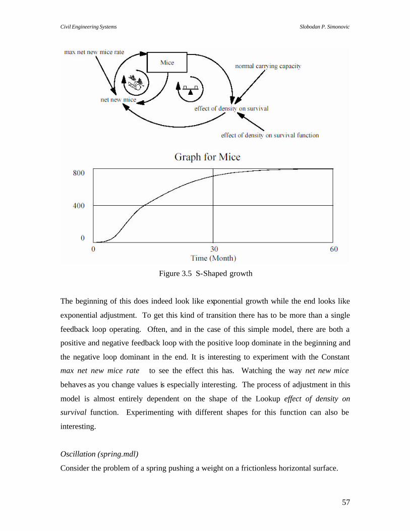
Civil Engineering Systems Slobodan P. Simonovic
57
Figure 3.5 S-Shaped growth
The beginning of this does indeed look like exponential growth while the end looks like
exponential adjustment. To get this kind of transition there has to be more than a single
feedback loop operating. Often, and in the case of this simple model, there are both a
positive and negative feedback loop with the positive loop dominate in the beginning and
the negative loop dominant in the end. It is interesting to experiment with the Constant
max net new mice rate to see the effect this has. Watching the way net new mice
behaves as you change values is especially interesting. The process of adjustment in this
model is almost entirely dependent on the shape of the Lookup effect of density on
survival function. Experimenting with different shapes for this function can also be
interesting.
Oscillation (spring.mdl)
Consider the problem of a spring pushing a weight on a frictionless horizontal surface.

Civil Engineering Systems Slobodan P. Simonovic
58
Figure 3.6 Oscillation
You need to be sure to use Runge-Kutta integration when simulating this model to get the
correct result. This is the simplest structure that can generate oscillations, and the
oscillations are undamped.
3.6 An Engineering System Dynamics Model Example
This section is focused on the conceptual issues in the development, analysis and use of a
model. After working through this example you should have a better understanding of
how to think about, and work through, a system dynamic simulation model with Vensim.
Background
You are involved in the production and sale of prefabricated window frames. Overall
your company is doing quite well, but you often go through periods of low capacity
utilization followed by production ramp up and added shifts. While all of this is normally
blamed on market demand and the condition of the economy, you have your doubts.
Looking back at sales and production over the last 8 years it seems that sales is more
stable than production. Your goal is to determine why this might be, and what you can
do about it. In attacking this problem you want to simplify as much as possible your
current situation. There are a number of reasons for this simplification:
• It is easier to understand a simple model.
• You can get results quickly and decide if you are on the right track.
• It is more effective to start with a simple model and add detail, than to build a
complex model and attempt to extract insights from it after it is complete.

Civil Engineering Systems Slobodan P. Simonovic
59
• Using a simple model forces you to take an overview which is usually useful in
the initial modeling phases.
It is not always true that you want to start building simple models. In many cases the
behavior you see is the result of complexity, and Vensim provides a very rich set of tools
for dealing with complexity. Until you have had substantial experience, however,
simplicity is highly recommended. While it is not uncommon to discover that what you
have developed is not rich enough for the problem you wish to address, it is rare not to
gain understanding in the process. Conversely, large complex models can become
significant resource drains, providing no payoff for a very long time.
Reference modes
A reference mode is a graphical statement about a problem. Verbally, the problem was
stated as "production is less stable than sales." Graphically we might draw:
Figure 3.7 Reference modes
This reference mode is a sketch of behavior we might expect a model to produce. It
might be real data from your records, or your expectation of what might happen in a new
situation. The reference mode is used to focus activity. Having mapped out one or more
reference modes the goal is to define the simplest structure that is sensible and capable of
generating patterns of behavior that qualitatively resemble the reference modes. If
appropriate, such a structure can also be refined in order to develop a model that can be
validated quantitatively against the available data.
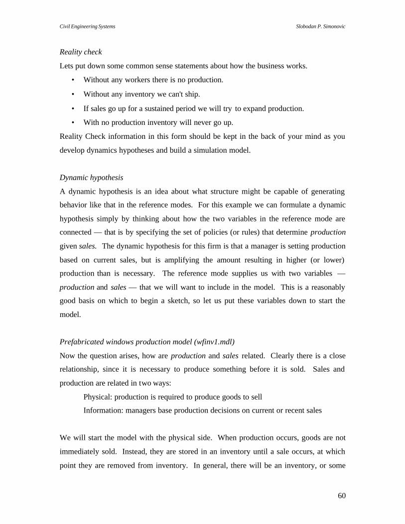
Civil Engineering Systems Slobodan P. Simonovic
60
Reality check
Lets put down some common sense statements about how the business works.
• Without any workers there is no production.
• Without any inventory we can't ship.
• If sales go up for a sustained period we will try to expand production.
• With no production inventory will never go up.
Reality Check information in this form should be kept in the back of your mind as you
develop dynamics hypotheses and build a simulation model.
Dynamic hypothesis
A dynamic hypothesis is an idea about what structure might be capable of generating
behavior like that in the reference modes. For this example we can formulate a dynamic
hypothesis simply by thinking about how the two variables in the reference mode are
connected — that is by specifying the set of policies (or rules) that determine production
given sales. The dynamic hypothesis for this firm is that a manager is setting production
based on current sales, but is amplifying the amount resulting in higher (or lower)
production than is necessary. The reference mode supplies us with two variables —
production and sales — that we will want to include in the model. This is a reasonably
good basis on which to begin a sketch, so let us put these variables down to start the
model.
Prefabricated windows production model (wfinv1.mdl)
Now the question arises, how are production and sales related. Clearly there is a close
relationship, since it is necessary to produce something before it is sold. Sales and
production are related in two ways:
Physical: production is required to produce goods to sell
Information: managers base production decisions on current or recent sales
We will start the model with the physical side. When production occurs, goods are not
immediately sold. Instead, they are stored in an inventory until a sale occurs, at which
point they are removed from inventory. In general, there will be an inventory, or some

Civil Engineering Systems Slobodan P. Simonovic
61
combination of inventory and backlog, separating production from sales. If a backlog is
used in the model, it is useful to consider orders and shipments instead of simply sales.
In this model, we will just use an inventory.
We construct Inventory as a Level, then add a rate flowing in and a rate flowing out.
Next, we use the variable merge tool to drag our two existing variables, production and
sales onto the valves.
Figure 3.8 Inventory part of the model
It is worth noting at this point that we could have created the same diagram by first
entering the level containing Inventory, then adding and naming the two rates. The
reason we chose to add Inventory then attach the existing variables as rates was to work
through the problem as it came to light, rather than working out the problem first then
putting it on the sketch.
Now we need to figure out how production gets determined. Over the long term
investment and capacity are clearly important, but these have been extremely stable. In
the shorter term more people are hired and, if necessary, an additional production shift
added. There is quite a bit of complicated stuff going on when shifts are added:
management changes, maintenance scheduling problems arise, and so on. However, as a
first approximation, more people make more products, and this is a good starting point,
so we add the level Workforce.
The things that change workforce are hiring, layoffs, firings and retirements. Again, for
simplicity we combine all of these into a composite concept — the net hire rate. Note
that net hire rate can either increase or decrease the workforce.
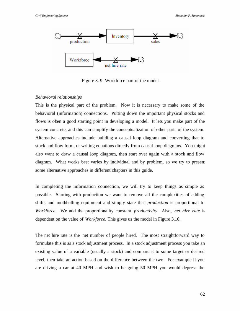
Civil Engineering Systems Slobodan P. Simonovic
62
Figure 3. 9 Workforce part of the model
Behavioral relationships
This is the physical part of the problem. Now it is necessary to make some of the
behavioral (information) connections. Putting down the important physical stocks and
flows is often a good starting point in developing a model. It lets you make part of the
system concrete, and this can simplify the conceptualization of other parts of the system.
Alternative approaches include building a causal loop diagram and converting that to
stock and flow form, or writing equations directly from causal loop diagrams. You might
also want to draw a causal loop diagram, then start over again with a stock and flow
diagram. What works best varies by individual and by problem, so we try to present
some alternative approaches in different chapters in this guide.
In completing the information connection, we will try to keep things as simple as
possible. Starting with production we want to remove all the complexities of adding
shifts and mothballing equipment and simply state that production is proportional to
Workforce. We add the proportionality constant productivity. Also, net hire rate is
dependent on the value of Workforce. This gives us the model in Figure 3.10.
The net hire rate is the net number of people hired. The most straightforward way to
formulate this is as a stock adjustment process. In a stock adjustment process you take an
existing value of a variable (usually a stock) and compare it to some target or desired
level, then take an action based on the difference between the two. For example if you
are driving a car at 40 MPH and wish to be going 50 MPH you would depress the

Civil Engineering Systems Slobodan P. Simonovic
63
accelerator. Your car's speed (a stock) will increase at a rate that depends on how far you
depress the accelerator and the car you are driving.
Figure 3.10 Connected model
To capture this stock adjustment process we add in the variables target workforce and
time to adjust workforce and connect them as shown :
Figure 3.11 Modified model
time to adjust workforce represents the time required for management to agree on a
change in the workforce level and screen potential applicants or notify workers to be laid

Civil Engineering Systems Slobodan P. Simonovic
64
off. target workforce is the number of people you need to produce the amount you want
to produce. The Level Workforce is initialized at this value. Now we add the concept of
target production, and connect it to target workforce. We will set target production on
the basis of sales.
Figure 3.12 Complete model
This is a complete model, though it does have a critical error of omission which will be
brought to light during simulation. The next step is to take the conceptual model and turn
it into a simulation model.
Equation set (wfinv1.vmf)
The full equation set for this model follows:
FINAL TIME =
100 Units:
Month
INITIAL TIME =
0 Units: Month
TIME STEP =
0.25 Units:
Month

Civil Engineering Systems Slobodan P. Simonovic
65
SAVEPER = TIME
STEP Units:
Month
Inventory =
INTEG(production
-sales, 300)
Units: Frame
net hire rate = (target workforce-Workforce)/time to adjust
workforce
Units:
Person/Month
production =
Workforce*productivity Units:
Frame/Month
productivity = 1
Units: Frame/Month/Person
sales = 100 +
STEP(50,20) Units:
Frame/Month
target production =
sales Units:
Frame/Month
target workforce = target
production/productivity Units: Person
time to adjust
workforce = 3 Units:
Month
Workforce = INTEG(
net hire rate, target
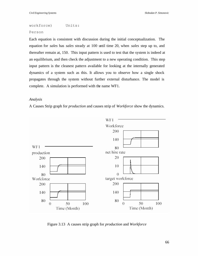
Civil Engineering Systems Slobodan P. Simonovic
66
workforce) Units:
Person
Each equation is consistent with discussion during the initial conceptualization. The
equation for sales has sales steady at 100 until time 20, when sales step up to, and
thereafter remain at, 150. This input pattern is used to test that the system is indeed at
an equilibrium, and then check the adjustment to a new operating condition. This step
input pattern is the cleanest pattern available for looking at the internally generated
dynamics of a system such as this. It allows you to observe how a single shock
propagates through the system without further external disturbance. The model is
complete. A simulation is performed with the name WF1.
Analysis
A Causes Strip graph for production and causes strip of Workforce show the dynamics.
Figure 3.13 A causes strip graph for production and Workforce
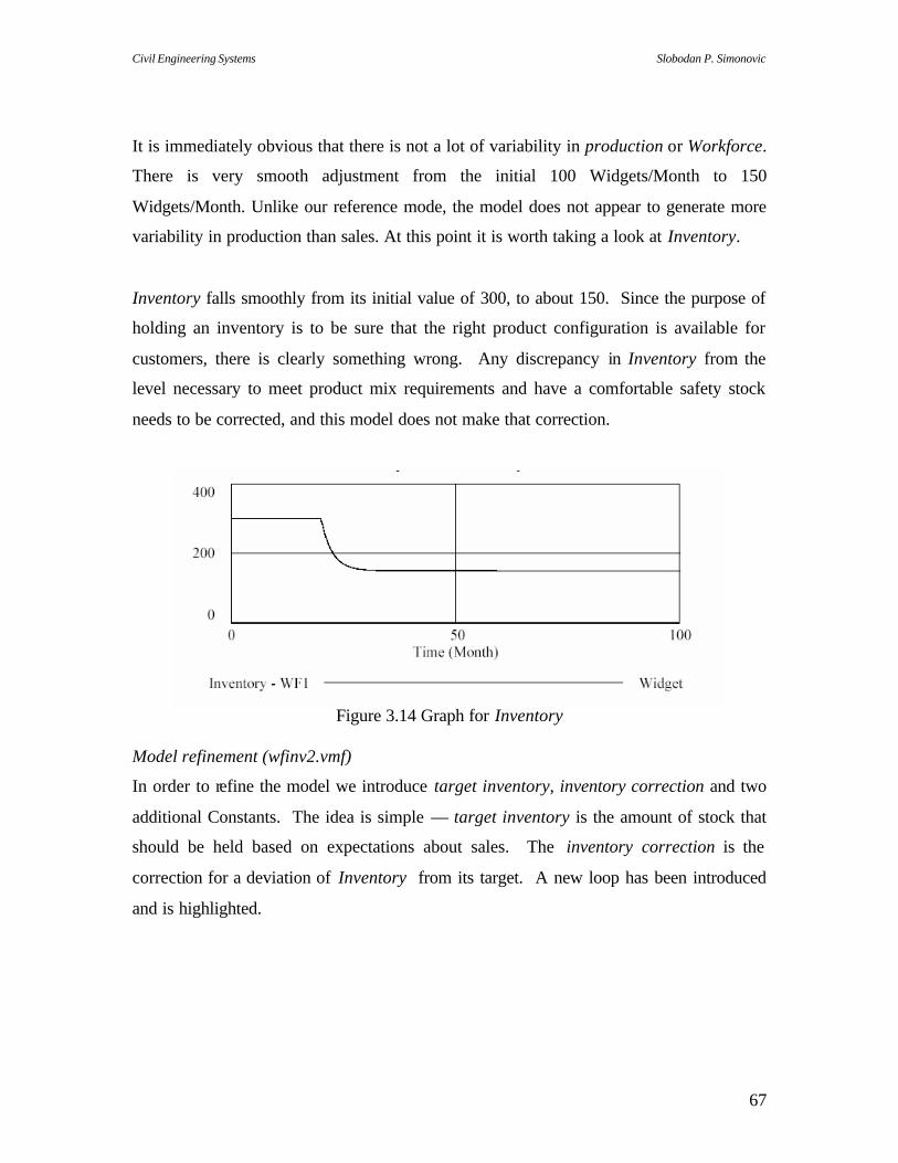
Civil Engineering Systems Slobodan P. Simonovic
67
It is immediately obvious that there is not a lot of variability in production or Workforce.
There is very smooth adjustment from the initial 100 Widgets/Month to 150
Widgets/Month. Unlike our reference mode, the model does not appear to generate more
variability in production than sales. At this point it is worth taking a look at Inventory.
Inventory falls smoothly from its initial value of 300, to about 150. Since the purpose of
holding an inventory is to be sure that the right product configuration is available for
customers, there is clearly something wrong. Any discrepancy in Inventory from the
level necessary to meet product mix requirements and have a comfortable safety stock
needs to be corrected, and this model does not make that correction.
Figure 3.14 Graph for Inventory
Model refinement (wfinv2.vmf)
In order to refine the model we introduce target inventory, inventory correction and two
additional Constants. The idea is simple — target inventory is the amount of stock that
should be held based on expectations about sales. The inventory correction is the
correction for a deviation of Inventory from its target. A new loop has been introduced
and is highlighted.
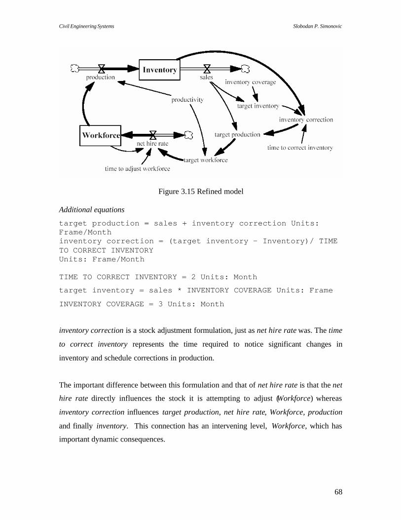
Civil Engineering Systems Slobodan P. Simonovic
68
Figure 3.15 Refined model
Additional equations
target production = sales + inventory correction Units: Frame/Month inventory correction = (target inventory - Inventory)/ TIME TO CORRECT INVENTORY Units: Frame/Month TIME TO CORRECT INVENTORY = 2 Units: Month
target inventory = sales * INVENTORY COVERAGE Units: Frame
INVENTORY COVERAGE = 3 Units: Month
inventory correction is a stock adjustment formulation, just as net hire rate was. The time
to correct inventory represents the time required to notice significant changes in
inventory and schedule corrections in production.
The important difference between this formulation and that of net hire rate is that the net
hire rate directly influences the stock it is attempting to adjust (Workforce) whereas
inventory correction influences target production, net hire rate, Workforce, production
and finally inventory. This connection has an intervening level, Workforce, which has
important dynamic consequences.

Civil Engineering Systems Slobodan P. Simonovic
69
Refined model behavior
The model is simulated and the run named WF2. First generate a graph of behavior for
Workforce with datasets from both runs loaded WF1 and WF2.
Figure 3.16 Refined model behavior
The behavior is dramatically different from the earlier model. Workforce is less stable
and there is oscillation. Causal tracing is performed on Workforce, and on target
workforce (graph not shown) and target production, and the output shown in Figure 3.17
below:
Figure 3.17 Causal tracing for the refined model

Civil Engineering Systems Slobodan P. Simonovic
70
inventory correction was not in the first model. Therefore there is no plot from WF1 for
inventory correction. All the oscillatory behavior in target production is due to inventory
correction. A graph of Inventory shows similar oscillation, but a different final value
from the first run. When sales increase, inventory now eventually adjusts to a new, higher
desired level, rather than falling as before.
Figure 3.18 Graph for Inventory for the refined model
Phasing and oscillation
To get some useful insight into this model, and oscillations in general, use the Graphs tab
in the Control Panel to create a graph containing Inventory, target inventory, production
and sales. Set the scales to zero minimum and 600 maximum values for all variables.
You will also need to go the Datasets tab of the Control Panel and put WF2 first.
Figure 3.19 Phasing and oscillation

Civil Engineering Systems Slobodan P. Simonovic
71
We want to focus in on the timing of changes just after the jump in sales. Hold down the
shift key and dragging across the portion of the graph of interest, or go to the Time Axis
tab of the Control panel, to set the time focus from approximately 18 months to 36
months. Now the custom graph generates this output:
Figure 3.20 Modified phasing and oscillation
Initially, when sales step up, inventory begins to fall because sales exceed production.
production gradually increases because target production increases with sales and
inventory correction increases as inventory falls. However, there is a delay in this process
due to the time required to hire new workers. By month 21.3, production is equal to sales,
so inventory stops falling and then begins to grow.
While Inventory is increasing, so is production. As long as inventory is below target
inventory, there is pressure to increase production, even when production is already
above sales. In fact, production needs to get sufficiently above sales so that the ongoing
difference balances the pressure from inventory correction before net hire rate will go
negative. Note that when Inventory is equal to target inventory, production is still higher
than sales because the workforce is excessive, causing an ongoing increase in Inventory.
The variability in production is now greater than that in sales; the model is exhibiting the
kind of amplification we identified in the reference mode.
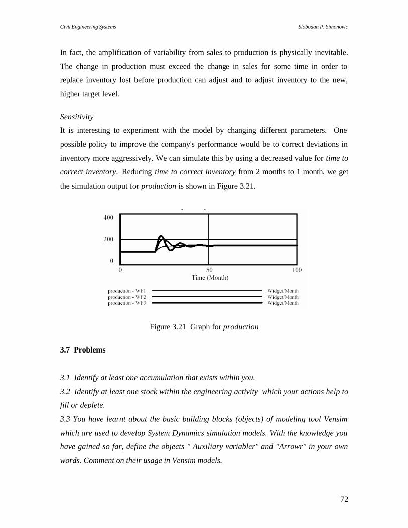
Civil Engineering Systems Slobodan P. Simonovic
72
In fact, the amplification of variability from sales to production is physically inevitable.
The change in production must exceed the change in sales for some time in order to
replace inventory lost before production can adjust and to adjust inventory to the new,
higher target level.
Sensitivity
It is interesting to experiment with the model by changing different parameters. One
possible policy to improve the company's performance would be to correct deviations in
inventory more aggressively. We can simulate this by using a decreased value for time to
correct inventory. Reducing time to correct inventory from 2 months to 1 month, we get
the simulation output for production is shown in Figure 3.21.
Figure 3.21 Graph for production
3.7 Problems
3.1 Identify at least one accumulation that exists within you.
3.2 Identify at least one stock within the engineering activity which your actions help to
fill or deplete.
3.3 You have learnt about the basic building blocks (objects) of modeling tool Vensim
which are used to develop System Dynamics simulation models. With the knowledge you
have gained so far, define the objects " Auxiliary variabler" and "Arrowr" in your own
words. Comment on their usage in Vensim models.

Civil Engineering Systems Slobodan P. Simonovic
73
3.4 I am teaching you what I know. Each of the following is a map of that process. For
each explain what you like and do not like about the map as a representation of the
process.
Things I know Things you know
teaching
Things I know 2 Things you know 2
learning
3.5 Create a simple Vensim sketch to represent each of the key feedback loop processes
described below:
(a) The activity of construction causes city to grow. As city grows and more
people come, construction also increases since there is more people.
(b) At the height of the Cold War, the nuclear arms race was a cause of great
public concern. Since neither the US nor the USSR had perfect knowledge of
the size of the other’s actual arsenal, neither side could be quite sure whether
they had ‘enough’ weapons relative to the other. When the US perceived that
the USSR had increased their arsenal the US stepped up its production of
weapons in order to keep up. Similar behavior is exhibited by the USSR.
(c) When John performs well in the class, his self-confidence grows. With this
increasing self-confidence comes even better performance.
3.6 Develop two simple Vensim models similar to the ones you have built in the first lab
session. Describe the problem you have chosen, stocks and flows, etc. Run the models
and generate results (just the graphs). Comment on the results based on the changes you
observe when you change the flow rates.
3.7 Use one of generic flow templates to represent each of the activities described below:
(a) Generation of noise pollution at the construction site;
(b) Regulation of room temperature with a thermostat; and
Civil Engineering Systems Slobodan P. Simonovic
74
(c) Generation of solid waste (optional: show the impact of recycling).
3.8 If you look at the model structure for the window manufacturing problem we have
developed in Section 3.6 you will see that it fails the Reality Check "Without Inventory we
can't ship." Try to develop a structure to correct this flaw. You will need to create an
explicit shipment variable and use a nonlinear function (Lookups are often used here) to
constrain shipments.
3.8 References
Lyneis, J., R. Kimberly, and S. Todd, (1994). “Professional Dynamo: Simulation Software
to Facilitate Management Learning and Decision Making,” in Modelling for Learning
Organizations, Morecroft, J., and J. Sterman, eds. Pegasus Communications.
Waltham, Massachusetts, USA.
Plummer, C. C., McGeary, D. (1991) Physical Geology, Fifth Edition. William C. Brown
Publishers, USA.
Powersim Corporation, (1996). Powersim 2.5 Reference Manual, Powersim Corporation
Inc., Herndon, Virginia, USA.
Sterman, J.D., (2000). Business Dynamics: Systems Thinking and Modeling for a Complex
World, McGraw Hill, New York, USA.
Ventana Systems, (1995). Vensim User’s Guide, Ventana Systems Inc., Belmont,
Massachusetts, USA.
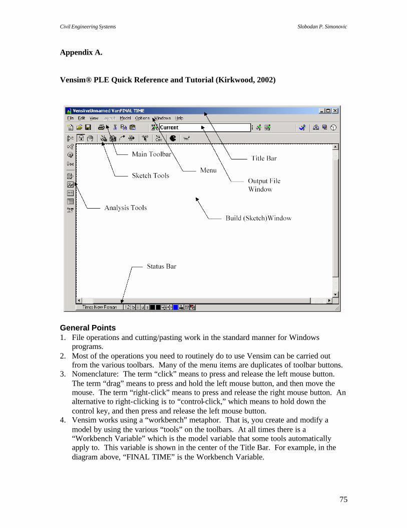
Civil Engineering Systems Slobodan P. Simonovic
75
Appendix A.
Vensim® PLE Quick Reference and Tutorial (Kirkwood, 2002)
General Points 1. File operations and cutting/pasting work in the standard manner for Windows
programs. 2. Most of the operations you need to routinely do to use Vensim can be carried out
from the various toolbars. Many of the menu items are duplicates of toolbar buttons. 3. Nomenclature: The term “click” means to press and release the left mouse button.
The term “drag” means to press and hold the left mouse button, and then move the mouse. The term “right-click” means to press and release the right mouse button. An alternative to right-clicking is to “control-click,” which means to hold down the control key, and then press and release the left mouse button.
4. Vensim works using a “workbench” metaphor. That is, you create and modify a model by using the various “tools” on the toolbars. At all times there is a “Workbench Variable” which is the model variable that some tools automatically apply to. This variable is shown in the center of the Title Bar. For example, in the diagram above, “FINAL TIME” is the Workbench Variable.

Civil Engineering Systems Slobodan P. Simonovic
76

Civil Engineering Systems Slobodan P. Simonovic
77

Civil Engineering Systems Slobodan P. Simonovic
78
Notes on the analysis tools: 1. The output of the analysis tools is “dead” in the sense that it does not change if you
make more simulation runs. Therefore, if you are doing experimentation, be careful that you keep track of what simulation run generated the output displayed in each output window.
2. Most output windows display information related to the Workbench Variable. You can select a variable to be the Workbench Variable by double-clicking on it in the Sketch. You can also select the Workbench Variable by double-clicking on a variable name in an output window.
3. The icons in the upper left corner of the output windows control various useful things. The horizontal bar at the left-most end deletes the window. The small padlock next to this is used to lock-out the delete function so that you do not accidentally delete the window. (Click this again to reactivate the delete function.) The small printer icon is used to print the contents of the window, and the clipboard icon is used to copy it into the Windows Clipboard. The floppy disk icon is used to save the window contents to a file.
4. For graph output when there are multiple curves on the same graph, the curves are displayed in different colors on the computer screen. With some black-and-white printers, it may be difficult to tell the curves apart in printed output. The curves can be marked with distinct numbers using the “Show Line Markers on Graph Lines” option on the “Options” menu.
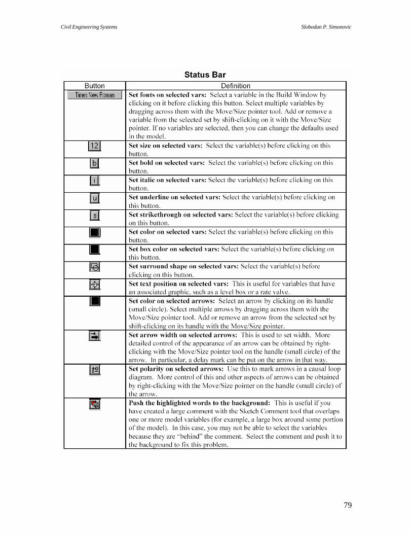
Civil Engineering Systems Slobodan P. Simonovic
79

Civil Engineering Systems Slobodan P. Simonovic
80
Highlights of the Menus Certain aspects of Vensim PLE can only be controlled by using menu items. This list shows some useful menu options:
1. Edit: There are “Find” options on this menu that can be used to track down all instances of a variable in a model sketch. This is useful when there are shadow (ghost) variables so that a variable can show up in more than one place in the model sketch.
2. View: The “Refresh” option repaints the computer screen. Certain computer video drivers have difficulty correctly responding to Windows graphics commands. This can result in “trash” on the screen (for example, an arrow that is not attached to anything, and that you cannot delete). Use the Refresh option to remove this trash. If this happens often, see item 4 below for a more permanent fix.
3. Model: The “Settings>Time Bounds tab” redisplays the “Time Bounds for Model” dialog that is displayed when you initially create a model. Use this dialog to change the time bounds variables (INITIAL TIME, FINAL TIME, TIME STEP, SAVEPER, and units for time).
4. Options: If you are continually having trash displayed on your computer screen (see item 2 above), then select the option “Continually Refresh Sketches.” This should eliminate the problem, but it may slow down working with sketches somewhat. If you cannot tell the different curves apart when you print more than one curve on the same graph, then select “Show Line Markers on Graph Lines” to have each curve marked with a different number.
5. Help: There is extensive online help for Vensim PLE
Miscellaneous Useful Items 1. With some printers, you may find that the curves for one or more arrows are not
shown in printed output of the model sketch. This can happen when the curve is almost, but not quite, a straight line. (It will be so close to a straight line that you may not be able to see the curvature on the computer screen.) Make sure that the curve is either truly a straight line or that it has visible curvature on the computer screen, and it should print all right.
2. Vensim can check units for your models. While it takes a little time to enter units for your equations, doing this can catch certain types of common errors (for example, using units of “days” one place and “weeks” somewhere else).
3. The Equation Editor is generally self-explanatory, but there is one useful point that is not immediately obvious; namely, how to enter a lookup function using the graphical dialog. When you start the Equation Editor on a variable that you wish to make into a lookup function, the “Type” of the variable will probably be shown as “Constant” in the left-center of the Equation Editor dialog. Drop down the type selection box and change the type to “Lookup.” After you do this, a new button labeled “As Graph” will appear in the dialog next to the “Help” button a couple of lines below the Type box. Click this to start the Graph Lookup definition dialog.

Civil Engineering Systems Slobodan P. Simonovic
81
In this tutorial, you will create the causal loop diagram shown above. Use the following steps:
1. Start Vensim, and click the New Model button on the Main Toolbar. The “Model Settings Time Bounds” dialog will display. You only need to worry about this for simulation models, so just click the “OK” button. A blank Build Window will appear. This is where you create your causal loop diagram. (A diagram in the Build Window is referred to as a “sketch.”)
2. Set the default font for this sketch to Arial 10 point, as follows: Click on the font name at the left end of the Status Bar. Since you do not have any items selected, the dialog will ask if you want to change the font and color defaults. Click the “Yes” button. The “View Defaults” dialog will be displayed. Change the “Face” to Arial and the “Size” to 10 points, and then click the “OK” button.
3. Select the “Variable - Auxiliary/Constant” tool from the sketch tools by clicking on it. Then click on the spot in the Build Window where you want to place the variable “interest.” An editing box will open. Enter “interest”, and press the “Enter” key. This word “interest” will appear on the sketch in Arial 10 point type. Repeat this process to create the variables “savings” and “income,” as shown in the diagram above. (Hints: If you discover that you have incorrectly spelled a variable name, select the “Variable - Auxiliary/Constant” tool, and click on the incorrectly spelled name. This will open the editing box for the variable. If you wish to completely remove a variable, or other element, from a sketch, select the “Delete” tool from the sketch tools, and click on the element to remove it.)
4. Repeat this process again to create the variable “work effort” shown in the diagram above. When you do this, both “work” and “effort” will appear on the same line. To put them on separate lines, as shown in the sketch above, place the tip of the mouse arrow on the small circle that is to the right and below the words “work effort,” and drag this circle with the mouse until “work” and “effort” are on separate lines. To change other characteristics of how “work effort” is displayed, do the following: Right-click (or, equivalently, control-click) on “work effort” in the sketch. A dialog box will open that provides a variety of options for how this variable is displayed. In the upper left section of this dialog, which is labeled “Shape,” note that the option “Clear Box” is selected. The small circle that you dragged to rearrange “work effort” is a “handle” that you use to change the shape of the Clear Box around “work effort.” Note that after you finish working on a variable with the “Variable – Auxiliary/Constant” tool the handle will disappear. When this happens, you can make the handle reappear by selecting the “Move/Size Words and Arrows” pointer tool from the sketch tools.

Civil Engineering Systems Slobodan P. Simonovic
82
5. Select the “Arrow” tool from the sketch tools by clicking on it. Then click on the variable “interest” in the Build Window, release the mouse button, and then click on the variable “savings.” A straight arrow will appear from “interest” to “savings.” Select the Move/Size pointer tool, and drag the handle (small circle) on this arrow to curve it as shown above. (Hint: As a shortcut, you can also drag using the Arrow tool. Put the tip of the curved arrow mouse pointer over the handle of the arrow in the sketch, and the curved arrow mouse pointer will change to a small hand. Then press the mouse button to drag.)
6. Repeat this process to draw arrows from “savings” to “interest,” “savings” to “work effort,” “work effort” to “income,” and “income” to “savings,” as shown in the sketch above. (Hints: You can speed up the process of creating a curved arrow by clicking with the Arrow tool at an intermediate point on the sketch between the variable names as you create the arrow. This will create a curved arrow in a single step. To remove an arrow, place the tip of the pointer on the “Delete” tool over the arrow’s head and click.)
7. You can move a variable by dragging it using the Move/Size tool. Note that as you move a variable, the arrows connected to that variable rearrange themselves to remain connected to the variable. (Hint: You can also drag a variable with the “Variable - Auxiliary/Constant” tool or the “Arrow” tool. Place the pointer of the tool over the variable name, hold down the left mouse button, and drag.)
8. Place a delay symbol on the arrow from “savings” to “work effort,” as shown in the sketch at the top of this tutorial, by right-clicking with the Move/Size tool on the arrow’s handle (small circle) in the Build Window, and then checking the “Delay marking” option in the upper center part of the dialog box that is displayed. (Hints: As a shortcut, you can also display this dialog box by right-clicking with the tip of the pointer for the “Arrow” tool cursor on the arrow’s handle. You can select more than one arrow at the same time by dragging the Move/Size pointer tool across their handles. You can add an additional arrow to the set of selected arrows by shift-clicking on its handle. When you select an arrow, its handle fills in.)
9. Add the plus signs shown in the sketch above to the arrows by selecting the arrows in the sketch as discussed in Step 8, and then clicking on the “Set polarity on selected arrows” button on the Status Bar. Select the plus sign from the displayed options. Follow an analogous procedure to add the minus sign to the arrow from “savings” to “work effort.”
10. You can change the positions of polarity signs by right-clicking on each arrow’s head or handle in turn and selecting the desired location from the “Position polarity mark at the” buttons at the bottom of the dialog. If you wish, you can also change the size of a plus or minus sign by changing the “Font” for the arrow from this same dialog.
11. Place the positive feedback loop symbol inside the positive feedback loop as follows: Select the “Sketch Comment” tool from the sketch tools by clicking it. Then click inside the positive feedback loop on the sketch. From the Comment Description dialog that opens, select a “Shape” of “Loop Clkwse.” Select “Image” under “Graphics,” and drop down the list of images to the right of this. Select the plus sign, and click on the “OK” button. The negative feedback loop symbol can be added to the sketch in an analogous manner with a “Shape” of “Loop Counter.”

Civil Engineering Systems Slobodan P. Simonovic
83
12. Finally, add the title “SAVINGS AND INCOME” by selecting the “Sketch Comment” tool, clicking on the sketch above the feedback loops, and entering “SAVINGS AND INCOME” into the “Comment” box. Change the font size to 12 points, and then click the “OK” button. Drag the handle of the Clear Box around this title to position all of the words on the same line.
13. Experiment with printing the diagram, and copying it into the Clipboard and then pasting it into a word processing document. Note that the printed or copied diagram does not have the handles (small circles) that may be shown on the sketch. Note that you must select the diagram to copy it into the Clipboard. You can do this by selecting “Select All” from the Edit menu, or by dragging across the entire diagram with the Move/Size pointer tool. (Hint: I f you use “Select All,” portions of curved arrows near the edge of the sketch may be chopped off in the copied diagram.)
14. If you wish, save your diagram using the “Save” button on the Main Toolbar. 15. Vensim PLE provides three analysis tools for analyzing the logical structure of a
causal loop diagram: “Causes Tree,” “Uses Tree,” and “Loops.” Specifically, the “Causes Tree” and “Uses Tree” tools show the variables that are causally connected to the current Workbench Variable in tree diagrams, while the “Loops” tool shows the causal (feedback) loops that contain the Workbench Variable.
16. Make sure that “savings” is selected as the Workbench Variable. The name of the Workbench Variable is shown following the rightmost colon on the “Title Bar.” If
“savings” is not selected as the Workbench Variable, select it by clicking on it in the sketch with the Move/Size tool. It will now be shown as the Workbench Variable on the Title Bar.
17. Click on the “Causes Tree” analysis tool. A window will open that displays the diagram shown in the left box below. Click on the “Uses Tree” analysis tool, and a window will open that displays the diagram shown in the right box below. These two tree diagrams trace backward and forward, respectively, through the causal link structure of the causal loop diagram starting at the current Workbench Variable, which is “savings.” Note that when a loop is completed back to the Workbench Variable, that variable’s name is shown in parentheses.
18. Make sure that “savings” is still selected as the Workbench Variable, and click on the
“Loops” analysis tool. The information shown below will be displayed. This is a list of all the causal (feedback) loops through the Workbench Variable.
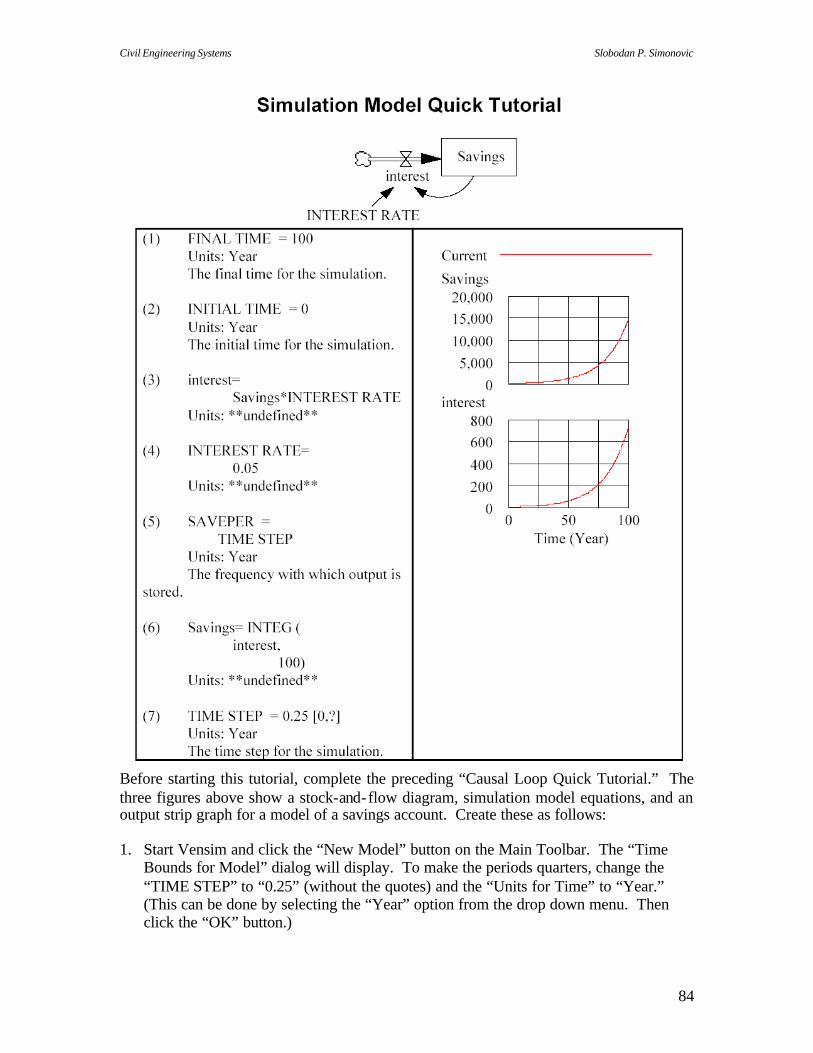
Civil Engineering Systems Slobodan P. Simonovic
84
Before starting this tutorial, complete the preceding “Causal Loop Quick Tutorial.” The three figures above show a stock-and-flow diagram, simulation model equations, and an output strip graph for a model of a savings account. Create these as follows:
1. Start Vensim and click the “New Model” button on the Main Toolbar. The “Time Bounds for Model” dialog will display. To make the periods quarters, change the “TIME STEP” to “0.25” (without the quotes) and the “Units for Time” to “Year.” (This can be done by selecting the “Year” option from the drop down menu. Then click the “OK” button.)

Civil Engineering Systems Slobodan P. Simonovic
85
2. Select “Box Variable -L evel” from the sketch tools, and click on the spot in the Build Window where you want “Savings” to appear. Enter “Savings” into the editing box that opens, and then press the “Enter” key. The “Savings” box will appear on the sketch.
3. Select the “Rate” tool from the sketch tools. Click to the left of the “Savings” box on the sketch in the Build Window, and release the mouse button. A cloud will appear on the sketch where you clicked. Move the mouse pointer to the “Savings” box and click. An editing box will appear. Enter “interest,” and press “Enter.” A flow pipe will now connect the cloud to the “Savings” box, and there will be a valve on this pipe with “interest” underneath, as shown in the stock-and-flow diagram at the top of this tutorial.
4. Select the “Variable - Auxiliary/Constant” sketch tool, and click on the spot in the Build Window where you want to place “INTEREST RATE.” Enter “INTEREST RATE into the editing box that opens, and press the “Enter” key. This variable now appears in the sketch.
5. Select the “Arrow” tool from the sketch tools, and draw arrows from “Savings” to “interest,” and from “INTEREST RATE” to “interest.” This completes the stock and flow diagram shown above.
Entering equations 6. Select the “Equations” tool from the sketch tools. The variables “interest,”
“INTEREST RATE,” and “Savings” will be highlighted in reverse video on the sketch. This highlighting signifies that these variables do not have valid equations assigned to them.
7. Click on “interest” in the sketch, and the “Editing equation for” dialog will open. Enter “Savings*INTEREST RATE” (without the quotes) into the box near the top of the dialog to the right of the equals sign. (Hint: You can “click in” this entire equation with the mouse using the keypad in the center of the dialog and the list of variable in the right-center of the dialog. For a simple equation like this one, this does not save much time over typing in the equation. However, it is a good idea to click in variable names so that you do not misspell them.) Click the “OK” button after you finish entering the equation.
8. If you have entered the equation correctly, the “Editing equation” dialog will close, and the “interest” variable will no longer show in reverse video on the sketch. In order to see how Vensim indicates an error in an equation, you may wish to spell “Savings” incorrectly in the equation. (Hint: You can click on a variable name in the sketch at any time the “Equations” tool is selected to edit the equation for that variable, even if you have already entered an equation for the variable.)
9. Click on “Savings” in the sketch, and the “Editing equation” dialog will open for “Savings.” Since Vensim is able to determine from the model sketch that the level of “Savings” is equal to the integral of “interest,” this equation is already shown next to the equal sign near the top of the dialog. Enter “100” (without the quotes) into the “Initial Value” box near the top of the dialog. As the name of this box indicates, it is for setting the initial value for “Savings.” Click the “OK” button to close the “Editing equation” dialog.

Civil Engineering Systems Slobodan P. Simonovic
86
10. Click on “INTEREST RATE” in the sketch, and enter “0.05” (without the quotes) into the box near the top of the dialog to the right of the equals sign. Click the “OK” button. You have now finished creating a model for a savings account that has an initial balance of 100 and an interest rate of 0.05 (that is, 5 per cent) per year. To show the equations for this model, select the “Document” tool from the analysis tools. The set of equations shown at the top of this tutorial will appear in a window.
Running a traditional simulation and displaying the results 11. Run the simulation model by clicking on the “Run a Simulation” button on the Main
Toolbar. I f a dataset named “Current” already exists on your computer, you will be shown a message
asking you whether you want to write over this. Answer “Yes” if this message appears. You will then momentarily see a dialog counting off the time as the simulation executes.
12. Make sure that “Savings” is selected as the Workbench Variable. The name of the Workbench Variable is shown following the rightmost colon on the “Title Bar.” If “Savings” is not selected as the Workbench Variable, select it by clicking on it in the sketch with the Pointer sketch tool. It will now be shown as the Workbench Variable on the Title Bar. Now select the “Causes Strip” tool from the analysis tools. The graphs for “Savings” and “interest” shown at the top of this tutorial will appear in a window.
13. You may wish to save your model using the “Save” button on the Main Toolbar. Also, you will find it useful to experiment with the “Build Windows - show/circulate” and “Output Windows - show/circulate” buttons on the Main Toolbar. Note that the Build Window containing the sketch of the stock-and-flow diagram is a standard window just like the Output Windows that show the model equations and the curves for the simulation output. All these windows act like normal Windows windows. In particular, if you click on an exposed part of the sketch in the Build Window while Output Windows also show on the computer screen, these Output Windows will vanish. What has happened is that the Build Window has been brought to the top of the stack of windows, and it now covers the Output Windows. You can bring the Output Windows back on top of the Build Window by clicking “Output Windows - show/circulate” on the Main Toolbar.
14. Conduct a sensitivity analysis for “INTEREST RATE” as follows: Click on the “Set up a Simulation” button on the Main Toolbar. When you do this, “INTEREST RATE” will be highlighted on the stock and flow diagram. This means that it is a constant which can be changed for a particular simulation run. Click on the highlighted “INTEREST RATE,” and an editing box will open showing the “INTEREST RATE” value of 0.05. Change this to 0.06, and press “Enter” to close the editing box. (Hint: Note that this change only applies to the next simulation run. After that, “INTEREST RATE” reverts to 0.05.)
15. Click the “Run a Simulation” button on the Main Toolbar. A dialog box will open saying “Dataset Current already exists. Do you want to overwrite it?” Answer “No.” Another dialog will open showing the datasets that are stored in the current directory. Enter “run2” for the “File name,” and press the OK button. The simulation now runs, and the results are stored in a new dataset file called “run2.vdf.”

Civil Engineering Systems Slobodan P. Simonovic
87
16. Make sure that “Savings” is selected as the Workbench Variable, and click the “Graph” button from the analysis tools. The graph shown on the next page will be displayed, except that the two curves will be shown in different colors, rather than marked by “1” and “2.” To add these markers, select “Options” on the “Menu,” and check the option “Show Line Markers on Graph Lines.” (Hint: If you print your graphs on a black and white printer, you will want to add these markers to better distinguish the curves in the printed output.)
17. Click on the “Runs Compare” analysis tool. This will display a window that shows the values of “INTEREST RATE” for the two simulation runs that have been completed.
18. You can change the display order of the curves on your graph, as well as add or delete curves from those shown on the graph. Do this by selecting “Control Panel” from the “Main Toolbar,” and then clicking on the “Datasets” tab. This shows the datasets that are currently “loaded” (that is, being used to create graphs) as well as other datasets that are available. A dataset can be “unloaded” by clicking on it in the list of “Loaded” datasets, and then clicking the double left-pointing arrow (<<). Once a dataset is unloaded, it will no longer be displayed when you create a graph until you reload it from the list of “Available” datasets by clicking it, and then clicking the double right-pointing arrow (>>). (Hints: The datasets are displayed on a graph in the order that they are listed in the “Loaded” list. If you click on a dataset that is not currently at the top of the “Loaded” list, this dataset will be moved to the top of the list. Note that any changes you make using the Control Panel options apply only to graphs that are created after you make these changes. All previously created graphs are “dead” in the sense that they do not change after they are created.)
19. You can create a table of values for the Workbench Variable by selecting the “Table” analysis tool. The “Table” window is “live,” unlike the graphical output windows.

Civil Engineering Systems Slobodan P. Simonovic
88
That is, as long as you leave this window open, each time you select the “Table” tool, the data for the current Workbench Variable is added to the data already in the “Table” window. (Hint: The “Table” tool is useful for creating data tables to be copied into a spreadsheet when you wish to create more complex graphical displays than is possible with Vensim. The “Table Time Down” analysis tool also creates a table for the Workbench Variable, but this table is arranged with values for different times in separate rows rather than separate columns.)
20. The causal loop analysis tools (“Causes Tree,” “Uses Tree,” and “Loops”) can be used to analyze the causal loop structure of a stock and flow diagram. Also, you can enter units for your variables in the equation editor. If you do this, then Vensim will check units for you.
21. You can control the time period used for simulation runs by selecting the “Time Bounds…” option from “Model>Settings” on the Menu. On the tab that is displayed for “Time Bounds…,” the “INITIAL TIME” entry sets the starting time for the simulation, and the “FINAL TIME” entry sets the ending time for the simulation. “TIME STEP” is the time interval at which new values are calculated for the model variables, and “SAVEPER” is the time interval at which the values are saved for the model variables. (Hints: The value of SAVEPER only impacts the interval at which the simulation results are saved for display in graphs or tables, and not the accuracy of the simulation calculations. SAVEPER should be set to an integer multiple of TIME STEP. If you set TIME STEP to a value less than one, then it is usually a good idea to set it to a power of 0.5, that is 0.5, 0.25, 0.125, 0.0625, etc. If TIME STEP is set to other values, then there may be roundoff error due to the way that computers store fractional numbers. The graphical display of simulation results can be controlled from the “Time Axis” tab of the “Control Panel” item on the Main Toolbar. Consult the online help for further information about this.)
Working with graphical sensitivity analysis (SyntheSim) 22. You can graphically view sensitivity of a model to the values of constants using a tool
called “SyntheSim.” When using SyntheSim, the results of the simulation are graphically overlaid on the model. Scales with bar sliders are used to represent changes that can be made to constants. Graphs are used to represent the output or impact on model variables.
23. Start SyntheSim by clicking on the “Automatically simulate on change” button on the Main Toolbar. If a dataset named “Current” already exists, you will be shown a message asking you whether you want to write over this. Answer “Yes” if this message appears. (See Step 28 for a full explanation.) You will then see the SyntheSim screen as shown below.

Civil Engineering Systems Slobodan P. Simonovic
89
24. New buttons appear on the Main Toolbar when using SyntheSim. The table below describes each SyntheSim button.
25. To see a variable graph in larger detail, hover the mouse pointer over the variable.
For instance, hover the mouse pointer over the “interest” variable. The larger graph is superimposed on the variable as shown below.
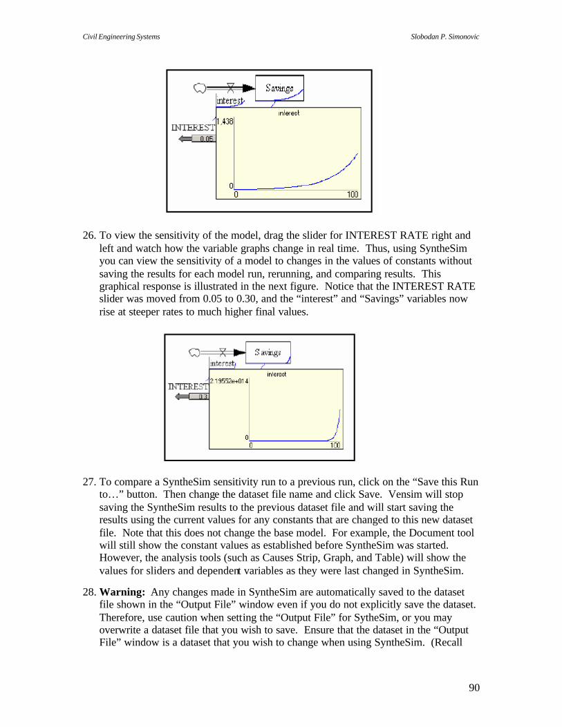
Civil Engineering Systems Slobodan P. Simonovic
90
26. To view the sensitivity of the model, drag the slider for INTEREST RATE right and left and watch how the variable graphs change in real time. Thus, using SyntheSim you can view the sensitivity of a model to changes in the values of constants without saving the results for each model run, rerunning, and comparing results. This graphical response is illustrated in the next figure. Notice that the INTEREST RATE slider was moved from 0.05 to 0.30, and the “interest” and “Savings” variables now rise at steeper rates to much higher final values.
27. To compare a SyntheSim sensitivity run to a previous run, click on the “Save this Run
to…” button. Then change the dataset file name and click Save. Vensim will stop saving the SyntheSim results to the previous dataset file and will start saving the results using the current values for any constants that are changed to this new dataset file. Note that this does not change the base model. For example, the Document tool will still show the constant values as established before SyntheSim was started. However, the analysis tools (such as Causes Strip, Graph, and Table) will show the values for sliders and dependent variables as they were last changed in SyntheSim.
28. Warning: Any changes made in SyntheSim are automatically saved to the dataset file shown in the “Output File” window even if you do not explicitly save the dataset. Therefore, use caution when setting the “Output File” for SytheSim, or you may overwrite a dataset file that you wish to save. Ensure that the dataset in the “Output File” window is a dataset that you wish to change when using SyntheSim. (Recall

Civil Engineering Systems Slobodan P. Simonovic
91
that when the SyntheSim simulation starts the prompt asks if it is ok to overwrite the current dataset. You can say no and change the dataset file name there—refer to Step 23).
29. To reset the constants in the model to their base model values, use either of the reset buttons. “Reset Current Slider to base model val” will reset only the selected constant slider to the value in the base model. “Reset all Constants/Lookups to base model vals” will reset all constant sliders to the values in the base model. 30. To stop SyntheSim, click the “Stop simulating” button. This will return you to the model definition view.
Working with custom graphs 31. You can create a custom graph by selecting “New…” on the “Graphs” tab of the
Control Panel, which is on the Main Toolbar. For example, suppose that you wish to display graphs of “Savings” and “interest” for both simulation runs “Current and “run2,” which you created earlier, on a single graph. There is no way to do this using the “Causes Strip” or “Graph” tools from the analysis tools.” However, you can create a custom graph that shows all four of these curves on a single graph.
32. To create this custom graph, select the “Control Panel” from the Main Toolbar, and then select the “Graphs” tab from the dialog that is displayed. To create a new custom graph, click the “New…” button in the lower right portion of the dialog, and the dialog shown at the top of the next page (but not yet filled in as shown in that figure) will be displayed. Using that figure as a guide, fill in the “Title,” and the entries shown on the “Variable” and “Dataset” columns in the lower portion of the dialog. The four entries in the “Variables” and “Datasets” columns specify which variables, from which simulation datasets, are to be displayed.
33. Finally, check the two boxes as shown under the entry “Scale” in the lower left portion of the dialog. Each checked box specifies that the variable immediately above the checked box and the variable immediately below the checked box are both to be displayed using the same scale on the vertical axis of the graph. Thus, with the boxes checked as shown in the figure on the next page, the two graphs for “Savings” are to be shown with the same vertical scale, and the two graphs for “interest” are to be shown with the same vertical scale (although the scales for the two pairs of graphs do not have to be the same). Click the “OK” button to close the custom graph definition dialog.

Civil Engineering Systems Slobodan P. Simonovic
92
34. You can display the custom graph that you have just defined by clicking the
“CUSTOM_GRAPH” entry on the Control Panel “Graphs” tab, and then clicking the “Display” button. When you do this, the graph below is displayed. Note that the vertical axis scale 40,000, 20,000, and 0 applies to the two graphs for “Savings,” while the vertical axis scale 4,000, 2,000, and 0 applies to the two graphs for “interest.” Further information about defining custom graphs is available in the online help.
Working with lookup functions 35. You can specify an arbitrary functional relationship between two variables in a
simulation model using a lookup function. To do this, you specify a table of pairs of values for the two variables, and Vensim uses linear interpolation to determine a value of the dependent variable for any value of the independent variable that is not specified in the table. To illustrate this approach, we will modify the savings account model developed above to consider a situation where there is a five percent interest

Civil Engineering Systems Slobodan P. Simonovic
93
rate on savings amounts less than $5,000, and a seven percent interest rate on savings amounts of $5,000 or greater.
36. Modify the stock and flow diagram for the savings account that you created earlier to create the stock and flow diagram shown below. To do this, change the constant name “INTEREST RATE” to “INTEREST LOOKUP.”
37. Use the “Equations” tool on the Main Toolbar to specify the lookup function equation
for “INTEREST LOOKUP.” To do this, open the equation editor on INTEREST LOOKUP. On the left side of the equation editing dialog, about two-thirds of the way up the dialog, there is an entry titled “Type” which shows “Constant” as the type of INTEREST LOOKUP. Click the arrow just to the right of the “Constant” to display a dropdown list of possible variable types. From this list, select “Lookup.” After you do this, a new button labeled “As Graph” will appear to the left of the “Help” button on the left side of the dialog below the “Type” entry.
38. Click on this “As Graph” button. When you do this, the Graph Lookup definition dialog will be displayed. You can enter a lookup function either by drawing it on the graph in the center of this dialog, or by entering pairs of numbers in the two column table on the left side of this dialog labeled “Input” and “Output”. Enter the lookup function using the Input and Output table as follows: In the first row of this table, enter 0 for Input and 0 for Output. In the
second row of this table, enter 5000 for Input and 250 for Output. In the third row of this table, enter 20000 for Input and 1300 for Output. Then click the “OK” button on the Graph Lookup definition dialog, and click the “OK” button on the equation editor. [What you have specified by these entries is that for an input (that is, “Savings”) of 0, the output (that is, “interest”) is 0, for an input of 5000, the output is 250, and for an input of 20000,
Civil Engineering Systems Slobodan P. Simonovic
94
the output is 1300. These are the correct values for the interest procedure specified in Step 35 above.]
39. Use the equation editor to specify the following equation for “interest:” INTEREST LOOKUP(Savings) This specifies that the value of “interest” for any value of “Savings” should be obtained by doing a linear interpolation between the values specified in INTEREST LOOKUP.
40. Run this simulation model, and display the Causes Strip graph for “Savings. You will obtain the results shown at the top of this page. As a check, you may wish to use the Table tool to obtain values for “Savings” and “interest.” The final value of “Savings” after 100 years should be 17,057, and the final value for “interest” should be 1,094. Comparing these strip graphs with the ones at the beginning of this section shows that the savings balance is somewhat higher after 100 years with the modified interest procedure, but the difference is not dramatic. This is because the higher interest rate does not start until the savings balance reaches $5,000, and that does not happen until year 78.
41. For further information about using lookup functions, consult the online help. While this example illustrates the use of lookup functions, it should be noted that the Vensim IF THEN ELSE function could also be used to calculate “interest” for this example. Consult the online help for information about IF THEN ELSE.
42. Finally, note that the Vensim sensitivity analysis feature can be used to temporarily change the shape of a lookup function for a particular simulation run.
Using “Time” as a variable 43. Some Vensim functions are explicit functions of time, and in order to use these
functions you must enter “Time” as a variable in your model. As an example, suppose that you wish to use a sine function with an amplitude of 100 units and a period of 12 months as a simple model of the seasonal variation component in demand for some product within a Vensim simulation model. Then a Vensim equation to represent this is
Variable Demand = 100 * sin(2 * 3.14159 * Time / 12) where Time is measured in months.
44. Press the New Model button to create a new Vensim simulation model. Make TIME STEP equal to 0.25, and leave the other time bounds for the model at their default values.
45. Use the “Variable – Auxiliary/Constant” tool to enter a variable called “Variable
Demand” (without the quotes) into your sketch for this model, and then attempt to use this tool to enter another variable called “Time” (also without the quotes) into this sketch. When you attempt to enter the variable Time, you will receive the following error message: “The variable Time already exists.” Click the OK button to clear this error message, and then press the Esc key to clear the variable entry box.
46. If you select the Document tool to examine the equations for your model, there will not be any variable called Time listed. However, even though it does not appear in

Civil Engineering Systems Slobodan P. Simonovic
95
the Document tool output, the variable Time is a built- in variable that exists in every Vensim simulation model.
47. Since Time already exists in the model, you enter it into the model sketch by using the “Shadow Variable” tool, rather than the “Variable – Auxiliary/Constant” tool. Select the Shadow Variable tool, click on the sketch where you want the variable Time to appear, and then select Time from the list of variables that is displayed. Then use the Arrow tool to draw an arrow from the Time variable to the Variable Demand variable. You will now have a sketch that looks something like the following:
(Note that Time appears in angle brackets to indicate that it is a shadow variable.)
48. Complete the model by using the Equations tool to enter the equation for Variable Demand shown above in item 34. Since Time is a shadow variable, do not enter an equation for it.
49. Press the “Run a Simulation” button to run the simulation model, make “Variable Demand” the Workbench Variable, and press the Causes Strip button. The following graph will be displayed:

Civil Engineering Systems Slobodan P. Simonovic
96
4. OPTIMIZATION BY CALCULUS
4.1 Introduction
In practice, Civil Engineers always have to make their designs conform to a variety of
constraints (De Neufville, 1990). They generally have to work within a budget. They
will have to satisfy engineering standards designed to ensure the quality, the
performance, and the safety of the system. They will also have to meet legal restrictions
the community has imposed to achieve its health and other objectives. The design of the
primary water supply system for New York City, for example, had to provide water at a
minimum pressure of 40 psi (pounds per square inch) as measured at the curb, with less
than a legal maximum for parts per million of various chemicals.
Constraints generally express some objectives for the system which could not be dealt
with analytically in an obvious way. Setting constraints on a system is an alternative to
the difficult problem of dealing explicitly with the multiple outputs of a system, which
has been very difficult to do. Thus New York City’s standard of 40 psi at the curb
represents an effort to ensure that the water pressure will be adequate for all residents of
the city.
The analysis will often demonstrate that many of these restrictions do not make much
sense in detail. They may easily cost far more to meet than is worth spending on the
objective they represent. New York’s standard of 40 psi for water pressure this entailed
enormous extra costs for the construction of its huge underground aqueducts. Tens of
millions of dollars could have been saved in the design if even slightly lower pressure
had been permitted in a few areas. While agreeing with the principle behind the
restrictions, in this case the idea that water pressure should be “adequate,” there is
generally much scope for improvements at the level of details (perhaps 38 psi would have
been a better standard than 40 psi).

Civil Engineering Systems Slobodan P. Simonovic
97
The reason that many restrictions on design do not make sense in details is that they were
never established on the basis of an analysis of the system. New York’s standard of 40
psi was certainly not based on a demonstration that it was the optimum level, or that it
was functionally preferable to 39 psi or 41 psi; it was almost certainly agreed to because
it was somewhere in the right region and because it was a nice round number.
Part of the Civil Engineer’s job in the future should be to help define the appropriate
levels of restrictions or, even better, to optimize the multiple output production process
directly. Meanwhile, however, the designer often will simply have to meet the
restrictions.
The difficulty in meeting restrictions on the design is that they complicate the
optimization process. To see this consider some function of many variables:
g(X) = g(X1, . . . ,Xi , . . . , Xn) (4.1)
which we assume to be continuous and analytic in that it has first and second derivatives.
If this function is unconstrained, the necessary conditions for its optimum (a maximum or
a minimum) is that all the first derivatives with respect to its arguments equal zero:
?g / ?Xi = 0 for all i (4.2)
On the other hand, if the function is constrained, these conditions for optimality may or
may not apply. The optimum may then be at the intersections of the function with the
constraint. Figure 4.1 makes the point. In a large scale system with hundred of variable
and constraints, the optimum could be located at an infinity of points.
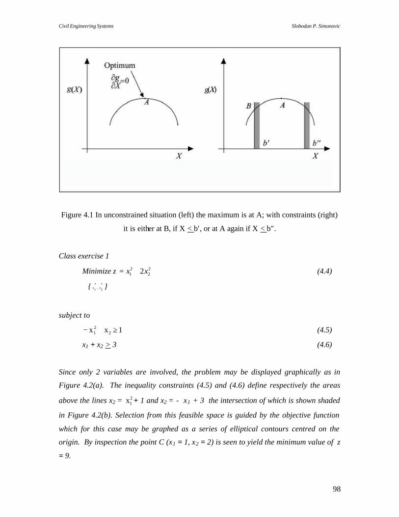
Civil Engineering Systems Slobodan P. Simonovic
98
Figure 4.1 In unconstrained situation (left) the maximum is at A; with constraints (right)
it is either at B, if X < b′, or at A again if X < b″.
Class exercise 1
Minimize z 22
21 2xx += (4.4)
{ *
2,*
1 xx }
subject to
1xx 221 ≥+− (4.5)
x1 + x2 > 3 (4.6)
Since only 2 variables are involved, the problem may be displayed graphically as in
Figure 4.2(a). The inequality constraints (4.5) and (4.6) define respectively the areas
above the lines x2 = 21x + 1 and x2 = - x1 + 3 the intersection of which is shown shaded
in Figure 4.2(b). Selection from this feasible space is guided by the objective function
which for this case may be graphed as a series of elliptical contours centred on the
origin. By inspection the point C (x1 = 1, x2 = 2) is seen to yield the minimum value of z
= 9.

Civil Engineering Systems Slobodan P. Simonovic
99
Figure 4.2 (a) Non-linear minimization in 2 variables. (b) Feasible space of Example 1.
(c) Feasible space of Example 2
Class exercise 2
Consider an example in which the signs of the constraints (4.5) and (4.6) are reversed,
i.e.
Minimize z 22
21 2xx +=
{ *
2,*
1 xx }
subject to
1221 ≤+− xx (4.7)

Civil Engineering Systems Slobodan P. Simonovic
100
x1 + x2 < 3 (4.8)
By comparison with the previous example it may be visualized that the feasible space
defined by (4.7) and (4.8) is the space below the line FBECG (Figure 4.2c). This space
includes the origin, which now forms the optimum (minimum) solution.
Class exercise 3
If the sign of the x2 term in (4.5) is changed, the feasible space is now defined by the
constraints:
21x + x2 < - 1 (4.9)
x1 + x2 > 3.
A brief examination shows that this feasible space is non-existent and no solution exists
to the minimization problem.
Therefore, it is clear that when a mathematical model includes inequality constraints:
(a) solution exists only if the constraints intersect to define a finite feasible space,
(b) the solution may lie on the edge of the feasible space, thus implying that at least one
of the constraints is active – i.e. affects the solution,
(c) the solution may lie in the interior of the feasible space, representing an
unconstrained optimization of the non-linear objective function.
Consider now some variation of the previous examples, to examine the significance of
equality constraints.
Class exercise 4
Assume that (4.5) is changed to an equality constraint. The problem now becomes
Minimize z 22
21 2xx +=
{ *
2,*
1 xx }
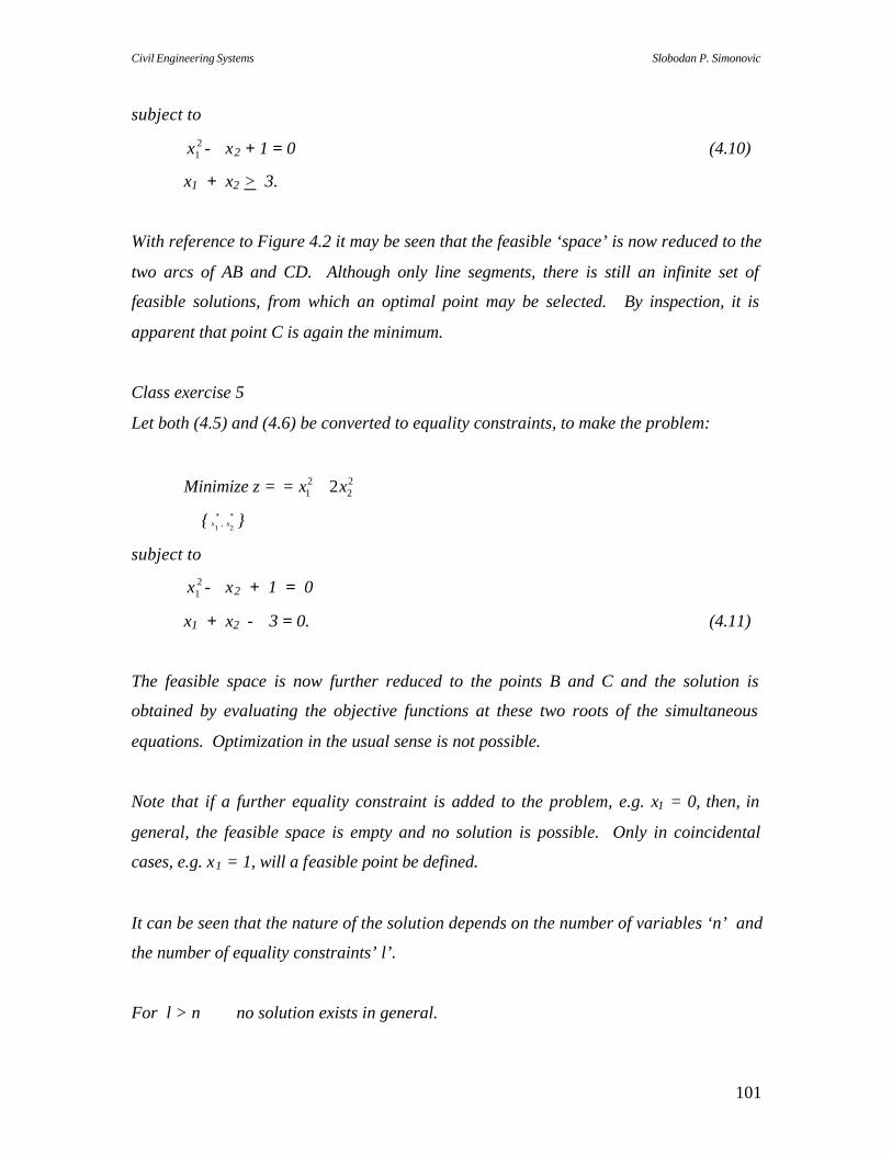
Civil Engineering Systems Slobodan P. Simonovic
101
subject to 21x - x2 + 1 = 0 (4.10)
x1 + x2 > 3.
With reference to Figure 4.2 it may be seen that the feasible ‘space’ is now reduced to the
two arcs of AB and CD. Although only line segments, there is still an infinite set of
feasible solutions, from which an optimal point may be selected. By inspection, it is
apparent that point C is again the minimum.
Class exercise 5
Let both (4.5) and (4.6) be converted to equality constraints, to make the problem:
Minimize z = 22
21 2xx +=
{ *
2,*
1 xx }
subject to 21x - x2 + 1 = 0
x1 + x2 - 3 = 0. (4.11)
The feasible space is now further reduced to the points B and C and the solution is
obtained by evaluating the objective functions at these two roots of the simultaneous
equations. Optimization in the usual sense is not possible.
Note that if a further equality constraint is added to the problem, e.g. x1 = 0, then, in
general, the feasible space is empty and no solution is possible. Only in coincidental
cases, e.g. x1 = 1, will a feasible point be defined.
It can be seen that the nature of the solution depends on the number of variables ‘n’ and
the number of equality constraints’ l’.
For l > n no solution exists in general.

Civil Engineering Systems Slobodan P. Simonovic
102
For l = n one or more discrete points (depending on the degree of the constraint
equations) are uniquely defined at which the objective function may be evaluated and a
solution obtained by inspection.
For l < n the feasible space (if it exists) may contain an infinite number of solutions
and an optimal solution, either on the edge or in the interior, must be determined by
search or other techniques.
In this connection it may be noted that any inequality constraint may be converted into an
equality constraint by the introduction of a slack variable. For example
- 21x + x2 > 1
is equivalent to
- 21x + x2 - x3 = 1. (4.12)
Thus a problem involving n decision variables, k inequality constraints, and l equality
constraints may be converted into a problem with (n + k) variables and (l + k) = m
equality constraints. The significance of the relative values of l and n discussed above is
therefore unaffected by the value of k.
4.2 Unconstrained functions
A single variable function
A function of a single variable may be examined by means of differential calculus (as
pointed in 4.1) to see if an extreme value (i.e. a maximum of minimum) exists. For this
to be possible the function must be: (i) continuous within the feasible domain of the
variable; (ii) differentiable once to locate critical points; and (iii) differentiable twice to
determine the sense of the critical points.
In general if a function z = F(x) exists then the values of x at which critical points may
exist are defined by setting the first derivative to zero, i.e.

Civil Engineering Systems Slobodan P. Simonovic
103
dz / dx = 0 (4.13)
Let one such solution of (4.13) be x*. Then the nature of the critical point is given by
evaluating the second derivative of z at x = x*. Thus for:
d2z / dx2 (x*) < 0 the critical point is a maximum
d2z / dx2 (x*) > 0 the critical point is a minimum.
Temporary lapses of memory in recalling this rule may be aided by the picture of Figure
4.3 in which the contents of an inverted or upright wine glass are considered as analogous
to the sign of the second derivative.
Figure 4.3 Wine-glass analogy
For the case in which the second derivative is zero at the stationary point some further
analysis is necessary. Find the lowest derivative which is non-zero at the stationary point,
i.e. dnz/dxn(x*) ? 0. If n is odd (n = 1, 3, 5,…) the solution found is a point of inflection
or a saddle point. If n is even (n = 2, 4,…) the rules of the wine-glass analogy may be
used as before.
Class exercise 6
Traffic passing through a road tunnel is causing a bottleneck and some form of access
control or speed control is considered as a means of maximizing the capacity. A survey
indicates that the headway (H miles) between vehicles is related to the speed (V mph) by
the empirical relation:
Civil Engineering Systems Slobodan P. Simonovic
104
H = 0.4/(50 – V) (4.14)
i.e.
density D (vehicles/mile) = 1/H = (50 – V)/0.4 (4.15)
or
D = 125 – 2.5V.
The traffic flow Q (vehicles/hour) is then given by:
Q = DV = 125V – 2.5V 2 (4.16)
The maximum flow is thus given by the critical point defined by
dQ/dV = 125 – 5V = 0 (4.17)
or
V* = 25 mph.
Since
d2Q/dV2 = – 5 < 0
the flow is a maximum when
Q = 125 * 25 – 2.5 * 252 = 1562.5 vehicles/hour.
Steps might be taken to maintain traffic speed as close to 25 mph as possible (by
controlling access). On the other hand, the headway at this speed (84.5 ft) seems
somewhat excessive and may be attributable to other factors such as poor illumination or
a greasy surface, which could be the real reason for the bottleneck.
A multiple variable function
Given a function

Civil Engineering Systems Slobodan P. Simonovic
105
F(x) where x = (x1, x2, …,xn)T (4.18)
for which all the first partial derivatives exist at all points within the feasible domain of
the function, a necessary condition for a stationary point is:
0=∂∂
ixF
i = 1, 2, …, n. (4.19)
Such a stationary point may be a minimum, a maximum, or a point of inflection.
Moreover, the possibility must be considered that two or more such stationary points may
exist.
In order to test the nature of the stationary point it is necessary to evaluate all the second
derivatives at the point, i.e.
?2F / ?xi ?xj i, j, = 1, 2, …, n. (4.20)
These second derivatives may be assembled in a Hessian matrix, thus:
∂∂
∂∂∂
∂∂∂
∂∂∂
∂∂
∂∂∂
∂∂∂
∂∂∂
∂∂
=
2n
2
2n
2
1n
2
n2
2
22
2
12
2n1
2
21
2
21
2
xF
...xx
Fxx
F............
xxF
...xF
xxF
xxF
...xx
FxF
H (4.21)
It will be noted that H is symmetric since:
ij
2
ji
2
xxF
xxF
∂∂∂
=∂∂
∂ (4.22)
Civil Engineering Systems Slobodan P. Simonovic
106
A sufficient condition for the stationary point to be a minimum is that all the second
derivatives exist at the point, and that all the principal minors are positive. (This implies
that H is positive-definite. The principal minors of a matrix A are defined as follows:
111 ap =
2221
12112 aa
aap =
…..
A=np (4.23)
where the symbol means ‘the determinant of’.
The corresponding condition that the stationary point is a maximum is that the even-
numbered principal minors (p2, p4,…) are positive and the odd-numbered principal
minors (p1, p3, p5,…) are negative. (This implies that H is negative-definite.) If
stationarity exists but the sufficient condition is not satisfied, then the nature of the point
is indeterminate and must be investigated by other means (e.g. numerical).
Another method of describing the sufficient condition is in terms of the eigen values of
the Hessian matrix evaluated at the stationary point. If all eigen values of the Hessian are
negative at x* then the stationary point is a local maximum. Clearly if all the eigen
values are negative for all possible values of x the point x* is a global maximum. If all
eigen values of the Hessian are positive at x* then the stationary point is a local
minimum. Similarly, the point is a global minimum if the eigen values are positive for all
possible values of x.
Civil Engineering Systems Slobodan P. Simonovic
107
4.3 Constra ined optimization
The practical problem is then to find ways to define optimality conditions which can
pinpoint the optimum when there are constraints. For analytic functions there are two
principal means of doing this, Lagrangeans and the Kuhn-Tucker conditions. The first is
explained in detail in following sections and the second one is out of the scope of this
course.
The purpose of this chapter is to provide insight into the nature of the optimal design of
constrained systems. It develops the key concept of ‘shadow price’ that is essential in the
practical application of optimization, particularly in sensitivity analysis. Optimization
problem with equality constraints solved by Lagrangeans, brings out the concept of
shadow prices.
Lagrangeans
Lagrangeans constitute the easiest solution to optimization subject to constraints.
Historically they are also the first. They may be considered an intermediate step to the
general optimality conditions published by Kuhn and Tucker in 1951.
Lagrangeans solve the problem of optimizing a function subject to equality constraints,
ones that must be met exactly. These routinely occur in practice. A standard example is
the requirement to use one’s budget entirely – otherwise it might be cut in the following
period. Formally, the Lagrangean addresses the problem of optimizing g(X) subject to a
series of constraints hj(X) = bj. Putting the matter into the standard vocabulary used with
optimization, we call the function to be optimized the objective function.
We then write the problem as:
Optimize: g(X)
Subject to: hj(X) = bj and X >0 (4.24)
Civil Engineering Systems Slobodan P. Simonovic
108
The condition that all X be positive is a standard assumption that in no way limits
practical applications: variables can always be redefined to meet this requirement. The
purpose of this condition is to simplify the second order, the sufficiency conditions of
optimality. In linear programming, discussed in Chapter 5, this sign convention is also
exploited to facilitate the optimization procedure.
The problem is solved by constructing a new function to be optimized. This is called the
Lagrangean and is:
L = g(X) - ∑ λj [hj(X) - bj] (4.25)
Each parameter λj is a constant associated with a particular equation, and is to be solved
for. These parameters are known as the Lagrangean multipliers.
The marvelous aspect of the Lagrangean is that it simultaneously permits us to optimize
g(X) and to satisfy the constraints hj(X) = bj. All we do is apply the conventional process
for unconstrained functions to the Lagrangean. The difference is that whereas in
considering g(X) we had i variables, one for each Xi, we now have (i + j) variables,
including one for each of the λj multipliers associated with the j constraints.
Applying the standard method of optimization to the Lagrangean we set all first
derivatives equal to zero and obtain:
?L / ?Xi = ?g / ?Xi - ∑jλj ?h / ?Xi = 0 (4.26)
?L / ?λj = hj(X) - bj = 0 (4.27)
The (i + j) set of Xi and λj that satisfy these (i + j) equations will determine the optimum.
This solution will be designated (X*, λ*) where the superscript * indicates optimality.

Civil Engineering Systems Slobodan P. Simonovic
109
Notice that the optimal solution to the Lagrangean clearly satisfies the constraints placed
on the original problem; they are identical to the ?L/?λj equations that help define the
optimal solution. Likewise, this solution also maximizes g(X) since, at optimality where
the constraints are met, the second term in the Lagrangean equals zero and optimizing L
is then equivalent to optimizing g(X) (see Class exercise 7).
Class exercise 7
Consider the problem:
Maximize:
g(X) = 3X1X22
Subject to:
h(X) = X1 + X2 = 3
X1 , X2 > 0
The Lagrangean is
L = 3X1X22 - λ(X1 + X2 - 3)
There is only one λ because there is only one constraint. There are (i + j) = 3 equations
defining the optimal solution. These are:
?L / ?X1 = 3X22 - λ = 0
?L / ?X2 = 6X1X 2 - λ = 0
?L / ?λ = X1 + X2 - 3 = 0
The first two equations imply that X2* = 2X1*. The third then leads to
X* = (1,2) and
λ* = 12
Civil Engineering Systems Slobodan P. Simonovic
110
The optimum is
g* (X) = 12.
The Lagrangean multiplier has a most important interpretation. It gives the systems
designer valuable information about the sensitivity of the results to changes in the
problems. At the optimum, the Lagrangean multiplier λj equals the rate of the change of
the optimum objective function g*(X) as the constraint bj = hj(X) varies. To see this,
take the partial derivative of the Lagrangean with respect to this constraint and obtain:
?L / ?bj = λj all j (4.27)
Now since the constraints are identically equal to zero at the optimum,
g*(X) = L (4.28)
and
?g* / ?bj = ?L / ?bj = λj all j (4.29)
In the vocabulary of economics and systems analysis, the Lagrangean multiplier is known
as the shadow price of the constraint. This neatly describes the parameter: it is the
implicit price to be paid, in terms of changes of g(X), per unit change of the constraint bj.
Being a derivative, the value of the shadow price in general varies with the value of the
constraint; the values calculated are thus instantaneous, at the margin, for any given value
of the constraint.
Semantic caution: Although the Lagrangean multiplier is called the shadow price, it has
no necessary connection with money. Its units are always in terms of those of the
function to be maximized, g(X), divided by those of the relevant constraint. Thus for the
design of New York city’s water supply system: when the objective was to maximize the
capacity to deliver water subject to constraints on the pressure, the shadow price of the
pressure standard was in terms of gallons per psi. The shadow price is expressed in terms

Civil Engineering Systems Slobodan P. Simonovic
111
of money only when g(X) is some monetary amount such as dollars of benefit from a
system.
The shadow price on a constraint is the quantitative indication of whether it is worthwhile
to alter this requirement. It is the information that allows the designer to judge to what
extent each of the constraints on a system make sense in detail. For New York City’s
water supply system, for example, the shadow price on the requirement that water be
delivered throughout the city at a minimum pressure of 40 psi at the curb was extremely
high; unless the community for some reason thought this was an absolutely vital
threshold, it would be reasonable to lower this standard for the areas of highest evaluation
so that the resulting improvements to the overall system could be shared by the whole
community.
This issue of sensitivity of the optimum to changes in the definition of the problem is one
of the central topics of all practical applications of systems analysis.
4.4 Problems
4.1 A rather old riveted, steel plate storage tank has an unfortunate habit of ‘popping’
corroded rivets, issuing a jet of water on the adjacent work area. A small wall is to be
located to retain the ponding. If the total depth is H determine the maximum distance x
from the tank wall where the jet may strike the ground.

Civil Engineering Systems Slobodan P. Simonovic
112
4.2 A rectangular, open-topped reservoir is to be proportioned. The flowrate, and thus
the cost of supplying water to the tank, is inversely proportional to the storage volume
provided. Typical figures are as follows:
Volume (m3) Flow (m3/s) Supply cost ($)
100 0.65 10 000
500 0.50 2000
1000 0.40 1000
2000 0.35 500
The cost of constructing the tank is based on the following rates: Base $2/m2; Sides
$4/m2; and Ends $6/m2. Find the dimensions for least cost. The supply cost may be
approximated by the function
c1 = 106/ Volume in m3.
4.3 Given the problem:
Maximize: Z = 2X + 3XY
Subject to: XY = X2/9 = 13
X, Y > 0
(a) Formulate the problem, state the optimality criteria and solve.
(b) What is the practical significance of the Lagrangean multiplier λ?
4.4 Assume that the number of highway miles that can be graded, H, is a function of
both the hours of labor, L, and of machines, M:
H = 0.5L0.2 M0.8

Civil Engineering Systems Slobodan P. Simonovic
113
(a) Minimize the cost of grading 20 miles, given that the hourly rates for labor and
machines are: CL = $20; CM = $160.
(b) Interpret the significance of the Lagrangean miltiplier.
4.5 A sedimentation tank is circular in plan with vertical sides above ground and a
conical hopper bottom below ground, the slope of the conical part being 3 vertically to 4
horizontally. Determine the proportions to hold a volume of 4070m3 for minimum area
of the bottom and sides.
4.6 Find the optimal reservoir size for irrigation. The total benefit (TB) derived
from irrigation water in a region has been estimated as
TB = 100 q - 0.0005 q2 (1)
where TB is expressed as dollars per year ($/yr) and q represents dependable water
supply, expressed in acre-feet per year (AF/yr).
Estimates of the annual total cost (TC) of a reservoir at different sizes results in the
expression

Civil Engineering Systems Slobodan P. Simonovic
114
TC = 44.42 q 0.90 + 0.098 q 1.45 (2)
where TC has units of dollars per year.
The agency responsible for reservoir construction wishes to maximize net benefit
(NB), defined as total benefit minus total cost. Algebraically,
Maximize NB(q) = TB(q) - TC(q). (3)
4.5 References
Baumol, W.J., (1977). Economic Theory and Operations Analysis, 4th ed., Prentice Hall,
Englewood Cliffs, NJ, USA.
de Neufville, R., (1990), Applied Systems Analysis: Engineering Planning and
Technology Management, McGraw Hill, New York, USA.
de Neufville, R., and Mira, L.-J., (1974). “Optimal Pricing for Air Transport Networks,”
Transportation Research, September, pp.1-11.
Jewell, T.K., (1986), A Systems Approach to Civil Engineering Planning and Design,
Harper and Row, New York, USA.
Winston, W.L., (1987). “Non-Linear Programming,” Ch. 11, Operations Research:
Applications and Algorithms, PWS Publishers, New York, USA.
Civil Engineering Systems Slobodan P. Simonovic
115
5. LINEAR PROGRAMMING (LP)
As indicated in Section 1 of this text, LP has been considered one of the most widely used
techniques in Civil Engineering. This section will introduce basic concepts of the linear
programming optimization technique (de Neufville, 1990; Hillier and Lieberman, 1990;
Jewell, 1986).
5.1 What is Linear Programming?
In many engineering decision problems, the aim is to maximize or minimize some objective,
but there are certain constraints on what can be done in optimising this objective. The term
linear programming (LP) is used to mean a way of modelling many of these problems so
that they have a special structure, and it also denotes the way of solving problems with such
a structure. It is a technique which can be applied in many different problem domains. The
first step in formulating a model, as discussed earlier, of the problem is to decide which are
the decision variables. These are the quantities which can be varied, and their variations
affect the value of the objective. The second step in the formulation is to express the
objective in terms of the decision variables. Lastly, in formulating the model, we must write
down the constraints that restrict the choices of our decision variables. The common sense
constraints are that we cannot make negative our decision variables. We can summarize the
mathematical representation of the LP model in the following way. Letting xj be the level of
Activity j, for j = 1, 2 ..., n, you want to select a value for each xj such that:
C1x1 + C2x2 + ... + Cnxn
is maximized, or minimized, depending on the context of the problem. The xj are
constrained by a number of relations, each of which is one of the following types:
a1x1 + a2x2 + ... + anxn ? = a
b1x1 + b2x2 + ... + bnxn = b
c1x1 + c2x2 + ... + cnxn =? c.

Civil Engineering Systems Slobodan P. Simonovic
116
The first relation includes the possible restriction xj ?= 0. Such a constrained optimization
problem may have:
(i) no feasible solution, that is, there may be no values of all the xj, for j = 1,
2,..., n, that satisfy every constraint;
(ii) a unique optimal feasible solution;
(iii) more than one optimal feasible solution; or
(iv) a feasible solution such that the objective function is unbounded; that is, the
value of the function can be made as large as desired in a maximization
problem, or as small in a minimization problem, by selecting an appropriate
feasible solution.
A simple reference problem
Let us consider the problem currently being analyzed by the management of Simon, Inc.,
a small manufacturer of bathroom tiles. Simon has been convinced by its distributor that
there is an existing market for both a medium and a high priced tiles. In fact, the
distributor is so confident of the market that if Simon can make the tiles at a competitive
price, the distributor has agreed to purchase everything Simon can manufacture over the
next three months.
After a thorough investigation of the steps involved to manufacture a tile, Simon has
determined that each tile produced will require the following operations:
1. preparing the material,
2. glazing,
3. finishing,
4. inspection and packaging.
The head of manufacturing has analyzed each of the operations and has concluded that if
the company produces a medium priced Standard model, each tile produced will require
107 of an hour in the preparation department, 2
1 of an hour in the glazing department, 1

Civil Engineering Systems Slobodan P. Simonovic
117
hour in the finishing department, and 101 of an hour in the inspection and packaging
department. Similarly, the more expensive Deluxe model will require 1 hour of
preparation time, 65 of an hour of glazing time, 3
2 of an hour of finishing time, and 41
of an hour of inspection and packaging time. This production information is summarized
in Table 5.1.
The accounting department has analyzed these production figures, assigned all relevant
variable costs, and has arrived at process for both types of tiles that will result in a profit
of $10 for every Standard tile produced and $9 for every Deluxe tile produced.
DEPARTMENTS
Product Preparation
Glazing Finishing Inspection & Packaging
Standard Tile 107 hr. 2
1 hr. 1 hr. 101 hr.
Deluxe Tile 1 hr. 65 hr. 3
2 hr. 41 hr.
Table 5.1 Production Operations and Production Requirements Per Tile
In addition, the head of manufacturing has studied his work load for the next three
months and estimates that he should have available a maximum of 630 hours of
preparation time, 600 hours of glazing time, 708 hours of finishing time, and 135 hours of
inspection and packaging time. Simon’s problem then is to determine how many
Standard and how many Deluxe tiles should be produced in order to maximize the profit.
If you were in charge of production scheduling for Simon, Inc., what decision would you
make given the above information? That is, how many Standard and how many Deluxe
tiles would you produce in the next three months?

Civil Engineering Systems Slobodan P. Simonovic
118
Changing the sense of the optimization
Any linear maximization model can be viewed as an equivalent linear minimization model,
and vice versa, by accompanying the change in the optimization sense with a change in the
signs of the objective function coefficients. Specifically,
and vice versa.
Changing the sense of an inequality
All inequalities in a linear programming model can be represented with the same directioned
inequality since:
and vice versa.
Converting an inequality to an equality
An inequality in a linear model can be represented as an equality by introducing a non-
negative variable as follows:
It is common to refer to a variable such as s as a slack variable, and t as a surplus variable.
x )c(- minimize as treatedbecan xc maximize jj
n
1j=jj
n
1j=∑∑
b,- x )a(- as written becan b xa jj
n
1j=jj
n
1j=
≥≤ ∑∑
0. t whereb =t 1- xa as written becan b xa
0 s whereb = s1+ xa as written becan b xa
jj
n
1j=jj
n
1j=
jj
n
1j=jj
n
1j=
≥≥
≥≤
∑∑
∑∑

Civil Engineering Systems Slobodan P. Simonovic
119
Converting equalities to inequalities
Any linear equality or set of linear equalities can be represented as a set of like-directioned
linear inequalities by imposing one additional constraint. The idea generalizes as follows:
where:
5.2 Canonical forms for linear optimization models
Sometimes it is convenient to be able to write any linear optimization model in a compact
and unambiguous form. The various transformations presented in the previous section
allow you to meet this objective, although it is now apparent that there is considerable
latitude in the selection of a particular canonical form to employ. We illustrate two such
representations here.
Any linear optimization model can be viewed as:
subject to
. x and m ..., 2, 1, = ifor b xa
as written becan m ..., 2, 1, = ifor b = xa
jj
n
1j=ijij
n
1j=
ijij
n
1j=
βα ≤≤ ∑∑
∑
.b - = and a - = i
m
1=iij
m
1=ij ∑∑ βα
xc maximize jj
n
1j=∑

Civil Engineering Systems Slobodan P. Simonovic
120
Similarly, any linear optimization model can be written as:
subject to:
It is typical, although not required, that n > m.
5.3 Geometric interpretation
There are two geometric representations of a linear optimization model. One is called the
solution space representation and is treated here. The other is called the requirements space
representation; it is less important for a beginner to understand.
Solution space representation - two dimensions (variables)
Here we proceed directly to the consideration of a numerical example:
maximize 12x 1 + 15x2 (5.1)
subject to
.n ..., 2, 1, = jfor 0 x
m ..., 2, 1, = ifor b xa
j
ijij
n
1j=
≥
≤∑
xc minimize jj
n
1j=∑
.n ..., 2, 1, = jfor 0 x
0) b( m ..., 2, 1, = ifor b = xa
j
iijij
n
1j=
≥
≥∑

Civil Engineering Systems Slobodan P. Simonovic
121
4x1 + 3x2 ? 12 (5.2)
2x1 + 5x2 ? 10 (5.3)
x1 ?= 0 and x2 ?= 0. (5.4)
The problem is graphed in Figure 5.1. Observe that both (5.2) and (5.3) are drawn as
equations. Then each inequality is indicated by an arrow on the side of the line representing
permissible values of x1 and x2. Since the two variables must be non-negative, the region of
permissible values is bounded also by the two coordinate axes.
Accordingly, the polygon oabc represents the region of values for x1 and x2 that satisfy all
the constraints. This polygon is called the solution set. The set points described by the
polygon is convex . The vertices 0, a, b, and c are referred to as the extreme points of the
polygon in that they are not on the interior of any line segment connecting two distinct
points of the polygon.
Figure 5.1 Solution space
The parallel lines in the figure represent various values of the objective function. The arrow
points in the direction of increasing values of the objective function. The optimal solution is
at the extreme point b, where x1 = 15/7, x2 = 8/7, and 12x1 + 15x2 = 300/7.

Civil Engineering Systems Slobodan P. Simonovic
122
Alternative optimal solutions
If the coefficients of the objective function are changed so as to alter the direction
of the parallel lines in Figure 5.1, it is clear that the optimal solution may change, but in any
case there is always an extreme-point optimal solution. Consider, in Figure 5.2 a problem
for one specific rotation of the parallel lines:
maximize 4x1 + 10x2 (5.5)
again subject to the same constraints (5.2), (5.3), and (5.4).
Now, all the points (an infinite number) on the segment ab are optimal. Thus x1 = 15/7 and
x2 = 8/7 are still optimal. But so are x1 = 0 and x2 = 2, as well as any positive-weighted
average of these two optimal solutions. The optimal value of the objective function is 20.
Figure 5.2 Alternative optimal solutions
Unbounded optimal solutions
The third illustration, shown in Figure 5.3 is based on the model:
maximize -2x1 + 6x2 (5.6)
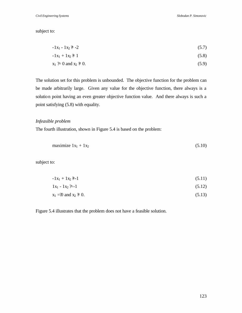
Civil Engineering Systems Slobodan P. Simonovic
123
subject to:
-1x1 - 1x2 ?= -2 (5.7)
-1x1 + 1x2 ?= 1 (5.8)
x1 ? = 0 and x2 ?= 0. (5.9)
The solution set for this problem is unbounded. The objective function for the problem can
be made arbitrarily large. Given any value for the objective function, there always is a
solution point having an even greater objective function value. And there always is such a
point satisfying (5.8) with equality.
Infeasible problem
The fourth illustration, shown in Figure 5.4 is based on the problem:
maximize 1x1 + 1x2 (5.10)
subject to:
-1x1 + 1x2 ?=-1 (5.11)
1x1 - 1x2 ? =-1 (5.12)
x1 =? 0 and x2 ?= 0. (5.13)
Figure 5.4 illustrates that the problem does not have a feasible solution.

Civil Engineering Systems Slobodan P. Simonovic
124
Figure 5.3 Unbounded solution Figure 5.4 Infeasible solution
Conclusion
We will summarize the results of the several geometric illustrations you have studied.
(i) If the solution set is nonempty, it is convex and may be either bounded or
unbounded.
(ii) If the solution set is nonempty, the optimal value of the objective function
may be finite or unbounded. If finite, then an optimal solution exists at an
extreme point.
5.4 Simplex method of solution
You will probably never have to calculate manually the solution of a linear programming
model in a real application, since a computer will do the work for you. You may
legitimately ask, then, "Why do I need to know the underlying theory of linear optimization
models? In the light of considerable experience in applying linear programming to
engineering problems, we are persuaded that an engineer must understand the principles
explained here in order to make truly effective and sustained use of this management tool.
Civil Engineering Systems Slobodan P. Simonovic
125
Many different algorithms have been proposed to solve linear programming problems, but
the one below has proved to be the most effective in general. The procedure appears to be
the following:
Step 1. Select a set of m variables that yields a feasible starting trial solution. Eliminate the
selected m variables from the objective function.
Step 2. Check the objective function to see whether there is a variable that is equal to zero
in the trial solution but would improve the objective function if made positive. If such a
variable exists, go to Step 3. Otherwise, stop.
Step 3. Determine how large the variable found in the previous step can be made until one
of the m variables in the trial solution becomes zero. Eliminate the latter variable and let the
next trial set contain the newly found variable instead.
Step 4. Solve for these m variables, and set the remaining variables equal to zero in the next
trial solution. Return to Step 2.
Interestingly, the resulting algorithm in fact does find an optimal solution to a general linear
programming model in a finite number of iterations. Often this method is termed Dantzig's
simplex algorithm, in honour of the mathematician who devised the approach.
We first examine a "well-behaved" problem and explain the simplex method by means of
this example. Afterwards we complete the presentation of the details.
Class exercise
Consider the model:
maximize 4x1 + 5x2 + 9x3 + 11x4
subject to:
1x1 + 1x2 + 1x3 + 1x4 ?= 15
7x1 + 5x2 + 3x3 + 2x4 ?= 120
3x1 + 5x2 + 10x3 + 15x4 ?= 100
x1 ?= 0 x2 =0 x3 =0 x4 ?= 0.
Civil Engineering Systems Slobodan P. Simonovic
126
Let x0 be the value of the objective function and add slack variables. Then write the system
as:
1x0 - 4x1 - 5x2 - 9x3 - 11x4 = 0 Row 0
1x1 + 1x2 + 1x3 + 1x4 + 1x5 = 15 Row 1
7x1 + 5x2 + 3x3 + 2x4 + 1x6 = 120 Row 2 (5.14)
3x1 + 4x2 + 10x3 + 15x4 + 1x7 = 100 Row 3,
where all the variables must be nonnegative. Notice how the introduction of the variable x0
in Row 0 permits us to express the objective function in equation form.
The task of Step 1 is to find a starting feasible solution to (5.14). There are a large number
of such solutions, but it is certainly most convenient to begin with x0 = 0, x5 = 15, x6 = 120,
x7 = 100, and all other variables equal to 0. In other words, start with an all-slack solution.
We term this an initial feasible basic solution, and x0, x5, x6, and x7 are known as the basic
variables, sometimes shortened to the basis. The remaining variables we call nonbasic.
Interpretation of coefficients in Row 0
Each coefficient represents the increase (for negative coefficients) or decrease (for positive
coefficients) in x0 with a unit increase of the associated nonbasic variable.
Iteration 1. For Step 2 the simplex method adopts the following easy-to-apply rule for
deciding the variable to enter the next trial basis.
Simplex Criterion I (maximization). If there are nonbasic variables having
a negative coefficient in Row 0, select one such variable with the most
negative coefficient, that is, the best per-unit potential gain (say xj). If all
nonbasic variables have positive or zero coefficients in Row 0, an optimal
solution has been obtained.
To decide which variable should leave the basic we will apply the following rule for Step 3.

Civil Engineering Systems Slobodan P. Simonovic
127
Simplex Criterion II. (a) Take the ratios of the current right-hand side to
the coefficients of the entering variable xj (ignore ratios with zero or negative
numbers in the denominator). (b) Select the minimum ratio - that ratio will
equal the value of xj in the next trial solution. The minimum ratio occurs for
a variable xk in the present solution; set xk = 0 in the solution.
The process of applying Criterion II is known as a change-of-basis calculation, or a pivot
operation. A detailed calculation is presented in Table 5.1.
Iteration 2. At this point the first iteration of the simplex method has been completed. On
returning to Step 2, you are ready to determine whether an optimal solution has been
obtained or if another simplex iteration is required. Criterion I, which examines the
nonbasic variables, indicates that a still better solution seems to exist. You might profitably
enter into the basis either x1, or x2, or x3. Criterion I selects x1, since it promises the greatest
gain per unit increase. Next perform the Step 3 calculations, using Criterion II. From Table
5.2, notice that x1 will replace x5 in the next trial solution.
Iteration 3. Having completed the second simplex iteration, once more examine the
coefficients in Row 0 to ascertain whether you have discovered an optimal solution. It now
appears favourable to enter x3 and remove x4 which was entered at the first iteration.
At this iteration you have just seen another aspect to the computational rule in Criterion II.
To sum up, Criterion II ensures that each new basic solution results only in zero or positive
values for the trial values of the basis. Consequently, the solution remains feasible at every
iteration.
Iteration 4. All the coefficients in Row 0 are nonnegative, and consequently Criterion I
asserts you have found an optimal solution. Thus the calculations are terminated in Step 2.
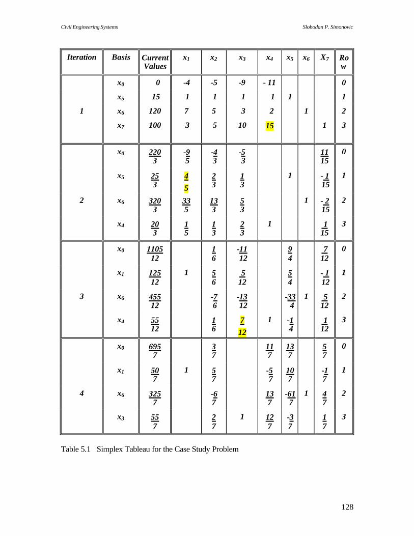
Civil Engineering Systems Slobodan P. Simonovic
128
Iteration Basis Current Values
x1 x2 x3 x4 x5 x6 X7 Row
x0 0 -4 -5 -9 - 11 0
x5 15 1 1 1 1 1 1
1 x6 120 7 5 3 2 1 2
x7 100 3 5 10 15
1 3
x0 220 3
-9 5
-4 3
-5 3
11 15
0
x5 25 3
4 5
2 3
1 3
1 - 1 15
1
2 x6 320 3
33 5
13 3
5 3
1 - 2 15
2
x4 20 3
1 5
1 3
2 3
1 1 15
3
x0 1105 12
1 6
-11 12
9 4
7 12
0
x1 125 12
1 5 6
5 12
5 4
- 1 12
1
3 x6 455 12
-7 6
-13 12
-33 4
1 5 12
2
x4 55 12
1 6
7 12
1 -1 4
1 12
3
x0 695 7
3 7
11 7
13 7
5 7
0
x1 50 7
1 5 7
-5 7
10 7
-1 7
1
4 x6 325 7
-6 7
13 7
-61 7
1 4 7
2
x3 55 7
2 7
1 12 7
-3 7
1 7
3
Table 5.1 Simplex Tableau for the Case Study Problem
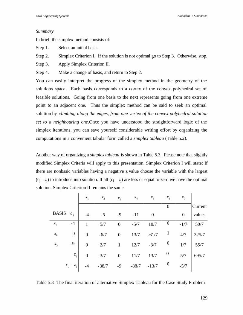
Civil Engineering Systems Slobodan P. Simonovic
129
Summary
In brief, the simplex method consists of:
Step 1. Select an initial basis.
Step 2. Simplex Criterion I. If the solution is not optimal go to Step 3. Otherwise, stop.
Step 3. Apply Simplex Criterion II.
Step 4. Make a change of basis, and return to Step 2.
You can easily interpret the progress of the simplex method in the geometry of the
solutions space. Each basis corresponds to a cortex of the convex polyhedral set of
feasible solutions. Going from one basis to the next represents going from one extreme
point to an adjacent one. Thus the simplex method can be said to seek an optimal
solution by climbing along the edges, from one vertex of the convex polyhedral solution
set to a neighbouring one.Once you have understood the straightforward logic of the
simplex iterations, you can save yourself considerable writing effort by organizing the
computations in a convenient tabular form called a simplex tableau (Table 5.2).
Another way of organizing a simplex tableau is shown in Table 5.3. Please note that slightly
modified Simplex Criteria will apply to this presentation. Simplex Criterion I will state: If
there are nonbasic variables having a negative zj value choose the variable with the largest
(cj – zj) to introduce into solution. If all (cj – zj) are less or equal to zero we have the optimal
solution. Simplex Criterion II remains the same.
1x 2x 3x 4x 5x 6x 7x
BASIS jc -4 -5 -9 -11 0
0
0
Current
values
1x -4 1 5/7 0 -5/7 10/7 0 -1/7 50/7
6x 0 0 -6/7 0 13/7 -61/7 1 4/7 325/7
3x -9 0 2/7 1 12/7 -3/7 0 1/7 55/7
jz 0 3/7 0 11/7 13/7 0 5/7 695/7
jc - jz -4 -38/7 -9 -88/7 -13/7 0 -5/7
Table 5.3 The final iteration of alternative Simplex Tableau for the Case Study Problem
Civil Engineering Systems Slobodan P. Simonovic
130
5.5 Completeness of the Simplex algorithm
In Criterion I, when two or more variables appear equally promising, as indicated by the
values of their coefficients in Row 0, an arbitrary rule may be adopted for selecting one of
these. For example, use the lowest-numbered variable, or one suspected to be in the final
basis.
In Criterion II, when two or more variables in the current basis are to fall simultaneously to
the level zero upon introducing the new variable, only one of these is to be removed from
the basis. The others remain in the basis at zero level. The resultant basis is termed
degenerate. A delicate question of theory is involved in the selection of a tie-breaking rule.
Unless some care is given to the method of deciding which variable is to be removed from
the basis, you cannot prove the method always converges. However, long experience with
simplex computations has led to the conclusion that for all practical purposes, the selection
can be arbitrary and the associated danger of nonconvergence is negligible.
If you find at some iteration in applying Criterion II that there is no positive coefficient in
any row for the entering variable, then there exists an unbounded optimal solution. In this
event, the entering variable can be made arbitrarily large, the value of x0 thereby increases
without bound, and the current basis variables remain nonnegative. Thus we now may drop
the earlier assumption that the optimal value of the objective function is finite. The simplex
algorithm provides an indication of when an unbounded optimal solution occurs. Criterion
II is easily reworded to cover this case.
Starting basis
Here we turn to the selection of an initial basis to begin the algorithm. Because each
constraint in the example of the preceding section was of the form:

Civil Engineering Systems Slobodan P. Simonovic
131
adding a slack variable to each relation and starting with an all-slack basic solution provided
a simple way of initiating the simplex algorithm. The constraints in any linear programming
model can be written as:
In this form, if a variable appears only in constraining relation i and has a coefficient of 1, as
would be the case for a slack variable, it can be used as part of the initial basis. But relation
i may not have such a variable. (This would occur, for example, if the ith equation were
linearly dependent on one or more of the other equations, such as being a sum of two
equations.) Then we may employ the following approach.
Write the constraints as:
and where yi ?= 0; then use yi as the basic variable for relation i. (We have assumed, for
simplicity, that every constraint requires the addition of a yi.) The name artificial variable is
given to yi because it is added as an artifice in order to obtain an initial-trial solution. Is this
approach legitimate? The answer is yes, provided you satisfy Condition A.
Condition A. To ensure that the final solution is meaningful, every yi must
equal 0 at the terminal iteration of the simplex method.
0, b whereb xa iijij
n
1j=
≥≤∑ (5.15)
0. b where m ..., 2, 1, = ifor b = xa iijij
n
1=j
≥∑ (5.16)
0, b where m ..., 2, 1, = ifor b = y1+ xa iiijij
n
1=j
≥∑ (5.17)

Civil Engineering Systems Slobodan P. Simonovic
132
The Big M method
There are a number of computational techniques for guaranteeing Condition A. One
approach is to add to the maximizing objective function each yi with a large penalty-cost
coefficient:
where M is relatively large. Thus each yi variable is very costly as compared to any of the xj
variables. To initiate the algorithm, you first eliminate each yi from (5.18) by using (5.17).
This gives:
which simplifies to:
Because the yi variables are so expensive, the very technique of optimizing drives the yi
variables to zero, provided there exists a feasible solution. (Incidentally, whenever a yi
drops from a basis at some iteration, you need never consider using it again, and can
eliminate it from further computations.) An example will clarify the approach.
Class exercise
Consider the problem:
maximize -3x1 - 2x2 (5.21)
subject to:
1x1 + 1x2 = 10 (5.22)
0, = My + xc - x i
m
1=ijj
n
1j=0 ∑∑ (5.18)
,b M- = xa M - xc - x i
m
1=ijij
n
1j=
m
1=ijj
n
1j=0 ∑∑∑∑ (5.19)
.b M- = x)a M + c( - x i
m
1=ijij
m
1=ij
n
1j=0 ∑∑∑ (5.20)
Civil Engineering Systems Slobodan P. Simonovic
133
1 x1 = 4 (5.23)
x1 ?= 0 x2 =? 0 (5.24)
Then, after adding a surplus variable x3 in (5.23), you can write the model as:
x0 + 3x1 + 2x2 = 0 Row 0
1x1 + 1x2 = 10 Row 1 (5.25)
1x1 - 1x3 = 4 Row 2.
Next, introduce artificial variables y1 and y2, and let M = 10, giving:
x0 + 3x1 + 2x2 + 10y1 + 10y2 = 0 Row 0
1x1 + 1x2 + 1y1 = 10 Row 1 (5.26)
1x1 - 1x3 + 1y2 = 4 Row 2.
To initiate the algorithm, you have to subtract (M = 10) times Row 1 and (M = 10) times
Row 2 from Row 0 to eliminate y1 and y2 :
x0 - 17x1 - 8x2 + 10x3 = -140 Row 0
1x1 + 1x2 + 1y1 = 10 Row 1 (5.27)
1x1 - 1x3 + 1y2 = 4 Row 2.
Verify that x1 = 4 and x2 = 6 are optimal.
5.6 Duality in LP
There is a unifying concept, namely duality, that establishes the inter-connections for all of
the sensitivity analysis techniques.

Civil Engineering Systems Slobodan P. Simonovic
134
Primal and dual problems
Consider the pair of linear programming models:
subject to:
and
subject to:
For the sake of definiteness, we arbitrarily call (5.28), (5.29), and (5.30) the primal problem
and (5.31), (5.32), and (5.33) its dual problem.
Class exercise
As an illustration, consider the following pair of problems:
maximize 4x1 + 5x2 + 9x3 (5.34)
subject to:
xc maximize jj
n
1j=∑ (5.28)
m ..., 2, 1, = ifor b xa ijij
n
1j=
≤∑ (5.29)
.n ..., 2, 1, = jfor 0 x j ≥ (5.30)
yb minimize ii
m
1=i∑ (5.31)
n ..., 2, 1, = jfor c ya jiij
m
1=i
≥∑ (5.32)
.m ..., 2, 1, = ifor 0 yi ≥ (5.33)

Civil Engineering Systems Slobodan P. Simonovic
135
1x1 + 1x2 + 2x3 ? =16
7x1 + 5x2 + 3x3 ?= 25 (5.35)
x1 ?= 0 x2 =? 0 x3 =0 Primal;
and
minimize 16y1 + 25y2 (5.36)
subject to:
1y1 + 7y2 =4
1y1 + 5y2 =5 (5.37)
2y1 + 3y2 ?= 9
y1 =0 y2 ?= 0 Dual.
Loosely put, the dual problem can be viewed as the primal model flipped on its side:
(i) The jth column of coefficients in the primal is the same as the jth row of
coefficients in the dual.
(ii) The row of coefficients of the primal objective function is the same as the
column of constants on the right-hand side of the dual.
(iii) The column of constants on the right-hand side of the primal is the same as
the row of coefficients of the dual objective function.
(iv) The direction of the inequalities and sense of optimization are reversed in the
pair of problems.
The proposition of significance is the following:
Dual Theorem
(a) In the event that both the primal and dual problems possess feasible solutions, then the
primal problem has an optimal solution x*j, for j = 1, 2, ..., n, the dual problem has an
optimal solution y*i, for i = 1, 2, ..., m, and

Civil Engineering Systems Slobodan P. Simonovic
136
(b) If either the primal or dual problem possesses a feasible solution with a finite optimal
objective function value, then the other problem possesses a feasible solution with the same
optimal objective-function value.
Primal (Maximize) Dual (Minimize)
Objective function Right-hand side
Right-hand side Objective function
jth column of coefficients jth row of coefficients
ith row of coeffic ients ith column of coefficients
jth variable nonnegative jth relation an inequality
jth variable unrestricted in sign jth relation an equality
ith relation an inequality ith variable nonnegative
ith relation an equality ith variable unrestricted in sign
Table 5.4 Relationship between primal and dual problems
5.7 Sensitivity Analysis
Sensitivity analysis is the study of how the optimal solution and the value of the optimal
solution to a linear program change given changes in the various coefficients of the
problem. That is, we are interested in answering questions such as the following:
(1) what effect will a change in the coefficients in the objective function (cj’s)
have?;
.yb = xc *ii
m
1=i
*jj
n
1j=∑∑ (5.38)
Civil Engineering Systems Slobodan P. Simonovic
137
(2) what effect will a change in the right-hand side values (bi’s) have?; and
(3) what effect will a change in the coefficients in the constraining equations
(aij’s) have? Since sensitivity analysis is concerned with how these
changes affect the optimal solution, the analysis begins only after the
optimal solution to the original linear programming has been obtained.
Hence, sensitivity analysis can be referred to as postoptimality analysis.
There are several reasons why sensitivity analysis is considered so important from an
engineering point of view. First, consider the fact that engineering businesses operate in
a dynamic environment. Prices of raw material change over time; companies purchase
new machinery to replace old; stock process fluctuate; employee turnovers occur; etc. If
a linear programming model has been used in a decision-making situation and later we
find changes in the situation cause changes in some of the coefficients associated with the
initial linear programming formulation, we would like to determine how these changes
affect the optimal solution to our original linear programming problem. Sensitivity
analysis provides us with this information without requiring us to completely solve a new
linear program. For example, if the profit for the Simon, Inc. Standard tiles were reduced
from $10 to $7 per tile, sensitivity analysis call tell the manager whether the production
schedule of 540 Standard tiles and 252 Deluxe tiles is still the best decision or not. If it
is, we will not have to solve a revised linear program with 21 97 xx + as the objective
function.
Sensitivity analysis can also be used to determine how critical estimates of coefficients
are in the solution to a linear programming problem. For example, suppose the
management of Simon, Inc. realizes the $10 profit coefficient for Standard tiles is a good,
but rough, estimate of the profit the tiles will actually provide. If sensitivity analysis
shows Simon, Inc. should produce 540 Standard tiles and 252 Deluxe tiles as long as the
actual profit for Standard tiles remains between $6.00 and $14.00, management can feel
comfortable that the recommended production quantities are optimal. However, if the
range for the profit of Standard tiles is $9.90 to $12.00, management may want to
reevaluate the accuracy of the $10.00 profit estimate. Management would especially

Civil Engineering Systems Slobodan P. Simonovic
138
want to consider what revisions would have to be made in the optimal production
quantities if the profit for Standard tiles dropped below the $9.90 limit.
As another phase of postoptimality analysis, management may want to investigate the
possibility of adding resources to relax the binding constraints. In the Simon, Inc.
problem, management would possibly like to consider providing additional hours (e.g.,
overtime) for the preparations and finishing operations. Sensitivity analysis can help
answer the important questions of how much will each added hour be worth in terms of
increasing profits and what is the maximum number of hours that can be added before a
different basic solution becomes optimal.
Thus, you can see that through sensitivity analysis we will be able to provide valuable
information for the decision maker. We begin our study of sensitivity analysis with the
coefficients of the objective function.
5.7.1 Sensitivity Analysis – The Coefficients of the Objective Function
In this phase of sensitivity analysis, we will be interested in placing ranges on the values
of the objective function coefficients such that as long as the actual value of the
coefficient is within this range, the optimal solution will remain unchanged. As stated in
the previous section, this information will tell us if we have to alter the optimal solution
when a coefficient actually changes, and will provide us with an indication of how
critical the estimates of the coefficients are in arriving at the optimal solution.
In the following sensitivity analysis procedures, we will be assuming that only one
coefficient changes at a time and that all other objective function coefficients remain at
the values defined in the initial linear programming model. To illustrate the analysis for
the coefficients of the objective function, let us again consider the final Simplex tableau
for the Simon, Inc. problem.
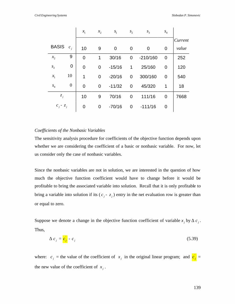
Civil Engineering Systems Slobodan P. Simonovic
139
1x 2x 1s 2s 3s 4s
BASIS jc 10 9 0 0 0 0
Current
value
2x 9 0 1 30/16 0 -210/160 0 252
2s 0 0 0 -15/16 1 25/160 0 120
1x 10 1 0 -20/16 0 300/160 0 540
4s 0 0 0 -11/32 0 45/320 1 18
jz 10 9 70/16 0 111/16 0 7668
jc - jz 0 0 -70/16 0 -111/16 0
Coefficients of the Nonbasic Variables
The sensitivity analysis procedure for coefficients of the objective function depends upon
whether we are considering the coefficient of a basic or nonbasic variable. For now, let
us consider only the case of nonbasic variables.
Since the nonbasic variables are not in solution, we are interested in the question of how
much the objective function coefficient would have to change before it would be
profitable to bring the associated variable into solution. Recall that it is only profitable to
bring a variable into solution if its ( jc - jz ) entry in the net evaluation row is greater than
or equal to zero.
Suppose we denote a change in the objective function coefficient of variable jx by ∆ jc .
Thus,
∆ jc = 'jc - jc (5.39)
where: jc = the value of the coefficient of jx in the original linear program; and 'jc =
the new value of the coefficient of jx .

Civil Engineering Systems Slobodan P. Simonovic
140
Using this notation, we can write the new objective function coefficient as
'jc = jc + ∆ jc (5.40)
It will be desirable to bring the nonbasic variable, jx , into solution if the new objective
function coefficient is such that 'jc - jz > 0 (i.e. if it will increase the value of the
objective function). On the other hand, we will not want to bring the variable jx into
solution, and thus, will not change our current optimal solution as long as 'jc - jz 0≤ .
Our goal in this phase of sensitivity analysis is to determine the range of values 'jc can
take on and still not affect the optimal solution.
Recall that jz is computed by multiplying the coefficients of the basic variables ( jc
column of the Simplex tableau) by the corresponding elements in the jth column of the A
portion of the tableau. Thus, a change in the objective function coefficient for a nonbasic
variable cannot affect the value of the jz ’s. Therefore, the values of 'jc that do not
require us to change the optimal solution are given by
'jc - jz 0≤ .
Since jz will be known in the final Simplex tableau, any new coefficient 'jc for a
nonbasic variable such that
'jc ≤ jz
will not cause a change in the current optimal solution.

Civil Engineering Systems Slobodan P. Simonovic
141
Note that there is no lower limit on the new coefficient 'jc . This is certainly as expected,
since we have a maximization objective function and thus lower and lower 'jc values will
make the nonbasic variables even less desirable.
Thus, for nonbasic variables, we can now establish a range of 'jc values which will not
affect the current optimal solution. We call this range the range of insignificance for the
nonbasic variables. It is given by:
jj zc ≤<∞− ' .
As long as the objective function coefficients for nonbasic variables remain within their
respective ranges of insignificance, the nonbasic variables will remain at a zero value in
the optimal solution. Thus, the current optimal solution and the value of the objective
function at the optimal solution will not change.
Coefficients of the Basic Variables
Let us start by asking the question of how much would the objective function coefficient
of a basic variable have to change before it would be profitable to change the current
optimal solution. Again, realize that we will only change the current optimal solution if
one or more of the net evaluation row values ( 'jc - jz ) becomes greater than zero.
Let us consider a change in the objective function coefficient for the basic variable 1x in
the Simon, Inc. problem. Let the new coefficient value be '1c . Using equation (5.40), we
can write '1c = 1c + 1c∆ where 1c is the original coefficient 10 and 1c∆ is the change in the
coefficient. Thus,
1'1 10 cc ∆+= (5.41)

Civil Engineering Systems Slobodan P. Simonovic
142
Let us now see what happens to the final Simplex tableau of the Simon, Inc. problem
where the objective function coefficient for 1x becomes 110 c∆+ . This tableau is as
follows:
1x 2x 1s 2s 3s 4s
BASIS jc 110 c∆+ 9 0 0 0 0
Current
value
2x 9 0 1 1630 0 160
210− 0 252
2s 0 0 0 1615− 1 160
25 0 120
1x 110 c∆+ 1 0 1620− 0 160
300 0 540
4s 0 0 0 3211− 0 320
45 1 18
jz 110 c∆+ 9 116
201670
c∆− 0 116
3016111
c∆+ 0
7668+540
1c∆
jc - jz 0 0 11620
1670
c∆+− 0 116
3016111
c∆−− 0
How does the change of 1c∆ affect our final tableau? First, note that since 1x is a basic
variable, the new objective function coefficient 1'1 10 cc ∆+= appears in the jc column of
the Simplex tableau. This means that the 110 c∆+ value will affect the jz values for
several of the variables. By looking at the jz row, you can see that the new coefficient
affects the jz values of the basic variable 1x , both nonbasic variables ( 1s and 3s ), and the
objective function.
Recall that a decision to change the current optimal solution must be based on values in
the net evaluation row. What variables have experienced a change in ( jc - jz ) values
because of the change 1c∆ ? As you can see, the change in the objective function

Civil Engineering Systems Slobodan P. Simonovic
143
coefficient for basic variable 1x has caused changes in the ( jc - jz ) values for both of the
nonbasic variables. The ( jc - jz ) values for all the basic variables remained unchanged;
( jc - jz ) = 0.
We have just identified the primary difference between the objective function sensitivity
analysis procedure for basic and nonbasic variables. That is, a change in the objective
function coefficient for a nonbasic variable only affects the jc - jz value for that variable;
however, a change in the objective function coefficient for a basic variable can affect the
jc - jz values for all nonbasic variables.
Returning to the Simon , Inc. problem with the coefficient for 1x changed to 110 c∆+ , we
know that our current solution will remain optimal as long as all ( jc - jz ) ≤ 0. Since the
basic variables all still have ( jc - jz ) = 0, we will have to determine what range of values
for 1c∆ will keep the ( jc - jz ) values for all nonbasic values less than or equal to zero.
For nonbasic variables 1s , we must have
116
2016
70 c∆+− 0≤ . (5.42)
Solving for 1c∆ , we see it will not be profitable to introduce 1s as long as
1670
1620
1 ≤∆c
2
7)1670(20
161 =≤∆c
.5.31 ≤∆c

Civil Engineering Systems Slobodan P. Simonovic
144
For nonbasic variables 3s , we must have
.01630
16111
1 ≤∆−− c (5.43)
Solving for 1c∆ , we see it will not be profitable to introduce 3s as long as
1630− 1c∆ ≤ 16
111
1630
1c∆ ≥ - 16111
1c∆ ≥ 3016
30111)16
111( −=−
1c∆ ≥ - 3.7.
Thus, in order to keep the net evaluation row values of the nonbasic variables less than or
equal to zero, and keep the current optimal solution, changes in 1c cannot exceed a 3.5
increase ( 1c∆ ≤ 3.5) or a 3.7 decrease ( 1c∆ ≥ - 3.7). Hence, our current solution will
remain optimal as long as:
-3.7 ≤ 1c∆ ≤ 3.5. (5.44)
From equation (5.41), we know that '11 cc =∆ - 10 where '
1c is the new value of the
coefficient for 1x in the objective function. Thus we can use equation (5.44) to define a
range for the coefficient values of 1x that will not cause a change in the optimal solution.
This is done as follows:
-3.7 ≤ '1c - 10 ≤ 3.5;

Civil Engineering Systems Slobodan P. Simonovic
145
therefore,
6.30 ≤ '1c ≤ 13.50.
The above result indicates to the decision maker that as long as the profit for one
Standard tile is between $6.30 and $13.50, the current production quantities of 540
Standard tiles and 252 Deluxe tiles will be optimal. We refer to the above range of
values for the objective function coefficient of 1x as the range of optimality for 1c .
To see how the management of Simon , Inc. can make use of the above sensitivity
analysis information, suppose that because of an increase in raw material prices, the
profit of the Standard tile is reduced to $7 per unit. The range of optimality for 1c
indicates that the current solution 1x = 540, 2x = 252, 1s = 0, 2s = 120, 3s = 0, 4s = 18
will still be optimal. To see the effect of this change, let us calculate the final Simplex
tableau for the Simon , Inc. problem after 1c has been reduced to $7.
1x 2x 1s 2s 3s 4s Current
vlaue
BASIS jc 7 9 0 0 0 0
2x 9 0 1 30/16 0 -210/160 0 252
2s 0 0 0 -15/16 1 25/160 0 120
1x 7 1 0 -20/16 0 300/160 0 540
4s 0 0 0 -11/32 0 45/320 1 18
jz 7 9 130/16 0 21/16 0 6048
jc - jz 0 0 -130/16 0 -21/16 0
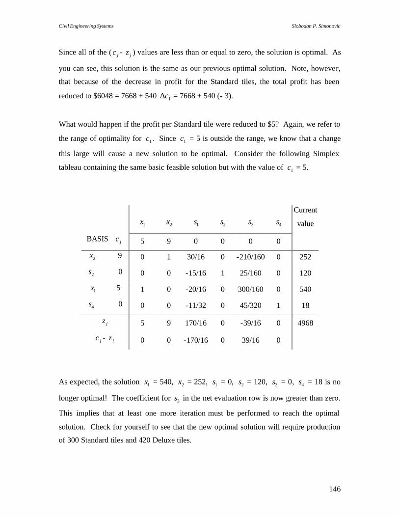
Civil Engineering Systems Slobodan P. Simonovic
146
Since all of the ( jc - jz ) values are less than or equal to zero, the solution is optimal. As
you can see, this solution is the same as our previous optimal solution. Note, however,
that because of the decrease in profit for the Standard tiles, the total profit has been
reduced to $6048 = 7668 + 540 1c∆ = 7668 + 540 (- 3).
What would happen if the profit per Standard tile were reduced to $5? Again, we refer to
the range of optimality for 1c . Since 1c = 5 is outside the range, we know that a change
this large will cause a new solution to be optimal. Consider the following Simplex
tableau containing the same basic feasible solution but with the value of 1c = 5.
1x 2x 1s 2s 3s 4s Current
value
BASIS jc 5 9 0 0 0 0
2x 9 0 1 30/16 0 -210/160 0 252
2s 0 0 0 -15/16 1 25/160 0 120
1x 5 1 0 -20/16 0 300/160 0 540
4s 0 0 0 -11/32 0 45/320 1 18
jz 5 9 170/16 0 -39/16 0 4968
jc - jz 0 0 -170/16 0 39/16 0
As expected, the solution 1x = 540, 2x = 252, 1s = 0, 2s = 120, 3s = 0, 4s = 18 is no
longer optimal! The coefficient for 3s in the net evaluation row is now greater than zero.
This implies that at least one more iteration must be performed to reach the optimal
solution. Check for yourself to see that the new optimal solution will require production
of 300 Standard tiles and 420 Deluxe tiles.

Civil Engineering Systems Slobodan P. Simonovic
147
Thus, we see how the range of optimality can be used to quickly determine whether or
not a change in the objective function coefficient of a basic variable will cause a change
in the optimal solution. Note that by using the range of optimality to determine whether
or not the change in profit coefficient for a basic variable is large enough to cause a
change in the optimal solution, we can avoid the time-consuming process of
reformulating and resolving the entire linear programming problem.
The general procedure for determining the range of optimality for the basic variable
associated with column j and row i of the Simplex tableau is to first find the range of
values for 1c∆ that satisfy
0)( ≤∆−−−
jikkk cazc (5.45)
for each nonbasic variable kx or ks . In this process, we will obtain a limit on jc∆ for
each nonbasic variable. The most restrictive upper and lower limits on jc∆ will be used
to define the range of optimality. For example, if one of these inequalities requires
jc∆ 3≤ and another requires jc∆ 1≤ , the jc∆ 1≤ is the most restrictive limit and will be
the upper limit for jc∆ .
After considering every nonbasic variable, we will have found upper and lower limits on
jc∆ in the following form:
βα ≤∆≤ jc
where: α = lower limit, and β = upper limit (α is ∞− if inequalities (5.45) do not
provide a lower limit on jc∆ and β is ∞+ if inequalities (5.45) do not provide an upper
limit).
Using the relationship )( 'jjj ccc −=∆ , the range of optimality is then given by

Civil Engineering Systems Slobodan P. Simonovic
148
βα ≤−≤ jj cc '
or
βα +≤≤+ jjj ccc ' (5.46)
Applying the above procedure to the objective function coefficient 2c in our Simon, Inc.
problem (the profit per unit for Deluxe tiles), we see that in order to satisfy inequalities
(5.45), 2c∆ must satisfy
0)1630()16
70( 2 ≤∆−− c (5.47)
and
0)1621()16
111( 2 ≤∆−− c . (5.48)
From (5.47), we get
37
2 −≥∆c .
And from (5.48), we get
21111
2 ≤∆c .
Thus we have
21111
37
2 ≤∆≤− c .
Using equation (5.46) and our original profit coefficient of 2c = 9, we have the following
range of optimality for 2c :
Civil Engineering Systems Slobodan P. Simonovic
149
2111193
79 '2 +≤≤− c
or
.29.1467.6 '2 ≤≤ c
Thus we see that as long as the profit of Deluxe tiles is between $6.67 per unit and $14.29
per unit, the production quantities of 540 Standard tiles and 252 Deluxe tiles will remain
optimal.
As a summary, we present the following managerial interpretation of sensitivity analysis
for the objective function coefficients. Think of the basic variables as corresponding to
our current product line and the nonbasic variables as representing other products we
might produce. Within bounds, changes in the profit associated with one of the products
in our current product line would not cause us to change our product mix or the amounts
produced, but the changes would have an effect on our total profit. Of course, if the
profit associated with one of our products changed drastically, we would change our
product line (i.e., move to a different basic solution). For products we are not currently
producing (nonbasic variables), it is obvious that a decrease in per unit profit would not
make us want to produce them; however, if the per unit profit for one of these products
became large enough, we would want to consider adding it to our product line.
5.7.2 Sensitivity Analysis – The Right-Hand Sides
A very important phase of sensitivity analysis, both from a theoretical and practical point
of view, is the study of the effect of changes of the right-hand sides on the optimal
solution and the value of the optimal solution. By changes of the right-hand sides, we
mean simply changing the values of one of the elements in the b vector in the matrix
representation of a linear program. We shall see that the Dual plays a role in this
analysis.

Civil Engineering Systems Slobodan P. Simonovic
150
Quite often in linear programming problems we can interpret the sbi ' as the resources
available. For example, in the Simon, Inc. problem, the right-hand side values
represented the number of man-hours available in each of four departments. Thus,
valuable management information could be provided if we knew how much it would be
worth to the company if one or more of these production time resources were increased.
Sensitivity analysis of the right-hand sides can help provide this information.
The Dual Variables as Shadow Prices
As we saw earlier in the section 5.6, in our study of the relationships between the Primal
and the Dual problems, there is a Dual variable associated with every constraint of the
Primal problem. It turns out that the values of these dual variables indicate how much the
value of the optimal solution to the Primal problem will change given a change in one of
the right-hand side values. This is another property if the relationships between the
Primal and Dual problems: If ib (the right-hand side of the ith primal cons traint) is
increased by one unit, the value of the optimal solution to the Primal problem will change
by iu units, where the iu is the value of the dual variable corresponding to the ith primal
constraint. We assume here that the same basis will remain optimal after making this
increase in ib . The reason for this assumption will be made clear later.
From the Primal-Dual relationship, we know that we can read the values of the optimal
dual variables for the Simon, Inc. problem from the final Simplex tableau of the Primal
problem.
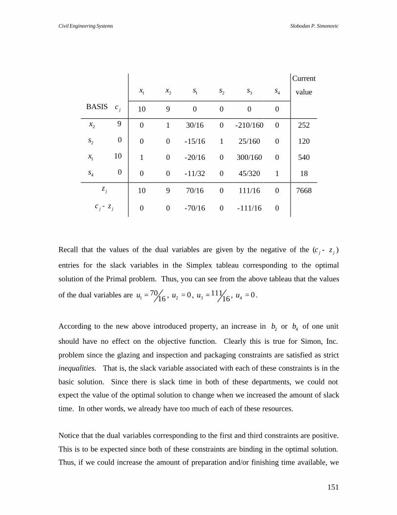
Civil Engineering Systems Slobodan P. Simonovic
151
1x 2x 1s 2s 3s 4s Current
value
BASIS jc 10 9 0 0 0 0
2x 9 0 1 30/16 0 -210/160 0 252
2s 0 0 0 -15/16 1 25/160 0 120
1x 10 1 0 -20/16 0 300/160 0 540
4s 0 0 0 -11/32 0 45/320 1 18
jz 10 9 70/16 0 111/16 0 7668
jc - jz 0 0 -70/16 0 -111/16 0
Recall that the values of the dual variables are given by the negative of the ( jc - jz )
entries for the slack variables in the Simplex tableau corresponding to the optimal
solution of the Primal problem. Thus, you can see from the above tableau that the values
of the dual variables are 1670
1 =u , 02 =u , 16111
3 =u , 04 =u .
According to the new above introduced property, an increase in 2b or 4b of one unit
should have no effect on the objective function. Clearly this is true for Simon, Inc.
problem since the glazing and inspection and packaging constraints are satisfied as strict
inequalities. That is, the slack variable associated with each of these constraints is in the
basic solution. Since there is slack time in both of these departments, we could not
expect the value of the optimal solution to change when we increased the amount of slack
time. In other words, we already have too much of each of these resources.
Notice that the dual variables corresponding to the first and third constraints are positive.
This is to be expected since both of these constraints are binding in the optimal solution.
Thus, if we could increase the amount of preparation and/or finishing time available, we

Civil Engineering Systems Slobodan P. Simonovic
152
could expect the value of the optimal solution to increase. The dual variable 1670
1 =u
indicates that the value of the optimal solution will increase by 1670 if 1b - the
maximum available preparation time – is increased by one unit. Similarly, the dual
variable 16111
3 =u indicates that the value of the optimal solution will increase by
16111 if 3b - the maximum available finishing time - is increased by one unit.
Let us consider the preparation operation in detail. Suppose we increase the original 630
hours available to 631 hours and then compute the revised final Simplex tableau. From
this tableau, which is shown below, we see that the objective function has increased by
1670 as expected.
1x 2x 1s 2s 3s 4s Current
value
BASIS jc 10 9 0 0 0 0
2x 9 0 1 30/16 0 -210/160 0 1614253
2s 0 0 0 -15/16 1 25/160 0 161119
1x 10 1 0 -20/16 0 300/160 0 1612538
4s 0 0 0 -11/32 0 45/320 1 322117
jz 10 9 70/16 0 111/16 0 1667672
jc - jz 0 0 -70/16 0 -111/16 0
You are probably wondering how this final tableau was computed. Certainly, we did not
go through all of the Simplex iterations again after changing 1b from 630 to 631. You
can see that the only changes in the tableau are the differences in the values of the basic
variables (i.e., the last column). The entries in this last column of the Simplex tableau

Civil Engineering Systems Slobodan P. Simonovic
153
have been obtained by merely adding the first five entries on the third column to the last
column in the previous tableau. That is,
=
+
−−−
166
3221
1612
161
1614
767217538119253
766818540120252
1670321116201615
1630
The reason for this is as follows. The entries in column 1s tell us how many units of the
basic variables will be driven out of solution if one unit of variable 1s is introduced into
solution. Increasing 1b by one unit has just the reverse effect. That is, it is just the same
as taking one unit of 1s out of solution. If 1b is increased by one unit, then the entries in
the 1s column tell us how many units of each of the basic variables may be added to
solution for every unit of 1s added. The increase in the value of the objective function
corresponding to adding one unit of 1b is equal to the negative of )( 33 zc − , or
equivalently, the value of the dual variable 1u .
Since this is such an important property, let us state it again. That is, associated with
every constraint of the Primal problem is a dual variable. The value of the dual variable
indicates how much the objective function of the Primal problem will increase as the
value of the right-hand side of the associated primal constraint is increased by one unit.
In other words, the value of the dual variable indicates the value of one additional unit of
a particular resource. Hence, this value can be interpreted as the maximum value or price
we would be willing to pay to obtain the one additional unit of the resource. Because of
this interpretation, the value of one additional unit of a resource is often called the
shadow price of the resource. Thus, the values of the dual variables are often referred to
as shadow prices.

Civil Engineering Systems Slobodan P. Simonovic
154
Range of Feasibility for the Right-Hand Side Values
The dual variables can be used to predict the change in the value of the objective function
corresponding to a unit change in one of the ib ’s. But here is the “catch”. The dual
variables can be used in this fashion only as long as the change in the ib ’s is not large
enough to make the current basis infeasible.
Thus, we will be interested in determining how much a particular ib can be changed
without causing a change in the current optimal basis. In effect we will do this by
calculating a range of values over which a particular ib can vary without any of the
current basic variables becoming infeasible. This range of values will be referred to as
the range of feasibility.
To demonstrate the effect of increasing a resource by several units, consider increasing
the available preparation time for the Simon, Inc. problem by 10 hours. Will the new
basic solution be feasible? If so, we can expect an increase in the objective function of
10 1u = 10 ( 1670 ) = $43.75. As before we can calculate the new values of the basic
variables by adding to the old values the change in ib times the coefficients in the 1s
column.
New solution =
=
−−−
+
169
168
1610
1612
3211
1620
1615
1630
14527110270
10
18540120252
Since the new solution is still feasible (i.e. all of the basic variable are 0≥ ), the
prediction made by the dual variable of a $43.75 change in the objective function
resulting from a 10-unit increase in ib is correct.
How do we know when a change in ib is so large that the current basis will become
infeasible? We shall first answer this question specifically for the Simon, Inc. problem.
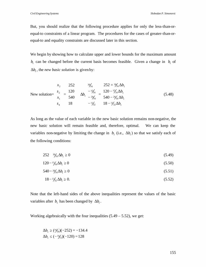
Civil Engineering Systems Slobodan P. Simonovic
155
But, you should realize that the following procedure applies for only the less-than-or-
equal-to constraints of a linear program. The procedures for the cases of greater-than-or-
equal-to and equality constraints are discussed later in this section.
We begin by showing how to calculate upper and lower bounds for the maximum amount
1b can be changed before the current basis becomes feasible. Given a change in 1b of
1b∆ , the new basic solution is given by:
New solution=
∆−∆−∆−
∆=
=
−−−
∆+
=
13211
11620
11615
11630
3211
1620
1615
1630
1
4
1
2
2
18540120
252
18540120252
bbb
b
b
sxs
x
(5.48)
As long as the value of each variable in the new basic solution remains non-negative, the
new basic solution will remain feasible and, therefore, optimal. We can keep the
variables non-negative by limiting the change in 1b (i.e., 1b∆ ) so that we satisfy each of
the following conditions:
0252 11630 ≥∆+ b (5.49)
0120 11615 ≥∆− b (5.50)
0540 11620 ≥∆− b (5.51)
.018 13211 ≥∆− b (5.52)
Note that the left-hand sides of the above inequalities represent the values of the basic
variables after 1b has been changed by 1b∆ .
Working algebraically with the four inequalities (5.49 – 5.52), we get:
128)120)((
4.134)252)((
1516
1
3016
1
=−−≤∆−=−≥∆
bb
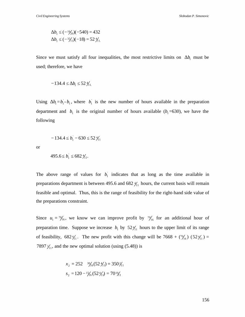
Civil Engineering Systems Slobodan P. Simonovic
156
.11
411
321
2016
1
52)18)((432)540)((
=−−≤∆=−−≤∆
bb
Since we must satisfy all four inequalities, the most restrictive limits on 1b∆ must be
used; therefore, we have
.114
1 524.134 ≤∆≤− b
Using 1b∆ = '1b - 1b , where '
1b is the new number of hours available in the preparation
department and 1b is the original number of hours available ( 1b =630), we have the
following
114'
1 526304.134 ≤−≤− b
or
495.6 .682 114'
1 ≤≤ b
The above range of values for '1b indicates that as long as the time available in
preparations department is between 495.6 and 682 114 hours, the current basis will remain
feasible and optimal. Thus, this is the range of feasibility for the right-hand side value of
the preparations constraint.
Since 1670
1 =u , we know we can improve profit by 1670 for an additional hour of
preparation time. Suppose we increase 1b by 11452 hours to the upper limit of its range
of feasibility, 114682 . The new profit with this change will be 7668 + ( 16
70 ) ( 11452 ) =
1117897 , and the new optimal solution (using (5.48)) is
112
114
1630
2 350)52(252 =+=x
1110
114
1615
2 70)52(120 =−=s
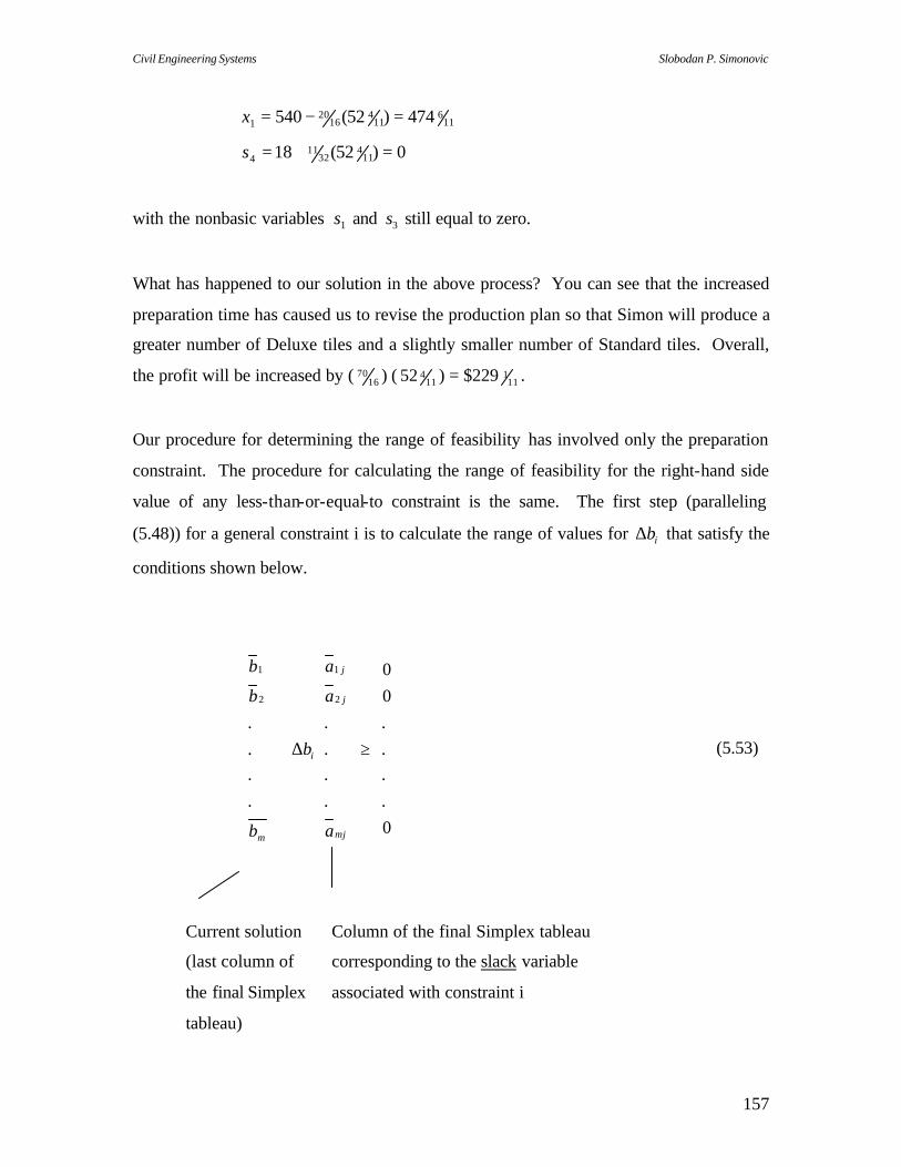
Civil Engineering Systems Slobodan P. Simonovic
157
116
114
1620
1 474)52(540 =−=x
0)52(18 114
3211
4 =+=s
with the nonbasic variables 1s and 3s still equal to zero.
What has happened to our solution in the above process? You can see that the increased
preparation time has caused us to revise the production plan so that Simon will produce a
greater number of Deluxe tiles and a slightly smaller number of Standard tiles. Overall,
the profit will be increased by ( 1670 ) ( 11
452 ) = $229 111 .
Our procedure for determining the range of feasibility has involved only the preparation
constraint. The procedure for calculating the range of feasibility for the right-hand side
value of any less-than-or-equal-to constraint is the same. The first step (paralleling
(5.48)) for a general constraint i is to calculate the range of values for ib∆ that satisfy the
conditions shown below.
≥
∆+
0....00
.
.
.
.
.
.
.
.2
1
2
1
mj
j
j
i
m a
a
a
b
b
b
b
(5.53)
Current solution Column of the final Simplex tableau
(last column of corresponding to the slack variable
the final Simplex associated with constraint i
tableau)
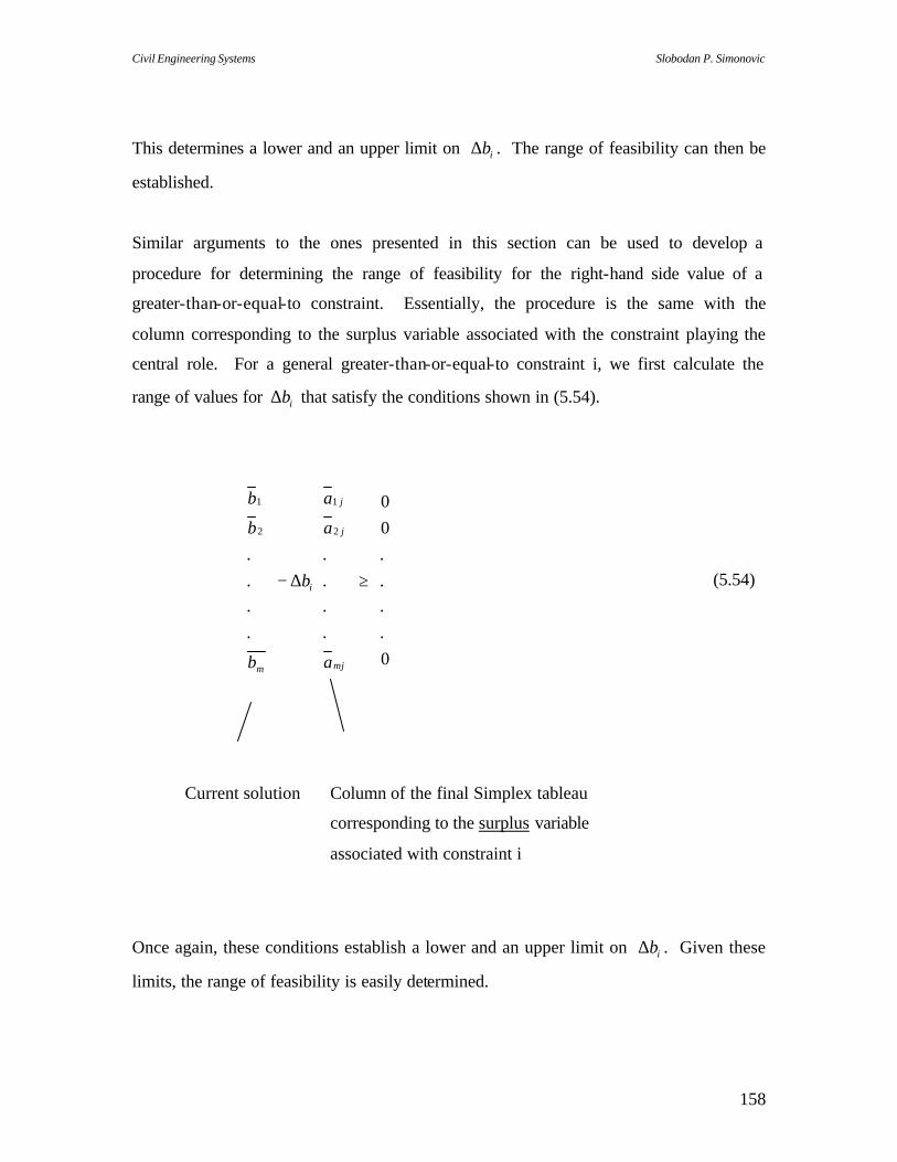
Civil Engineering Systems Slobodan P. Simonovic
158
This determines a lower and an upper limit on ib∆ . The range of feasibility can then be
established.
Similar arguments to the ones presented in this section can be used to develop a
procedure for determining the range of feasibility for the right-hand side value of a
greater-than-or-equal-to constraint. Essentially, the procedure is the same with the
column corresponding to the surplus variable associated with the constraint playing the
central role. For a general greater-than-or-equal-to constraint i, we first calculate the
range of values for ib∆ that satisfy the conditions shown in (5.54).
≥
∆−
0....00
.
.
.
.
.
.
.
.2
1
2
1
mj
j
j
i
m a
a
a
b
b
b
b
(5.54)
Current solution Column of the final Simplex tableau
corresponding to the surplus variable
associated with constraint i
Once again, these conditions establish a lower and an upper limit on ib∆ . Given these
limits, the range of feasibility is easily determined.
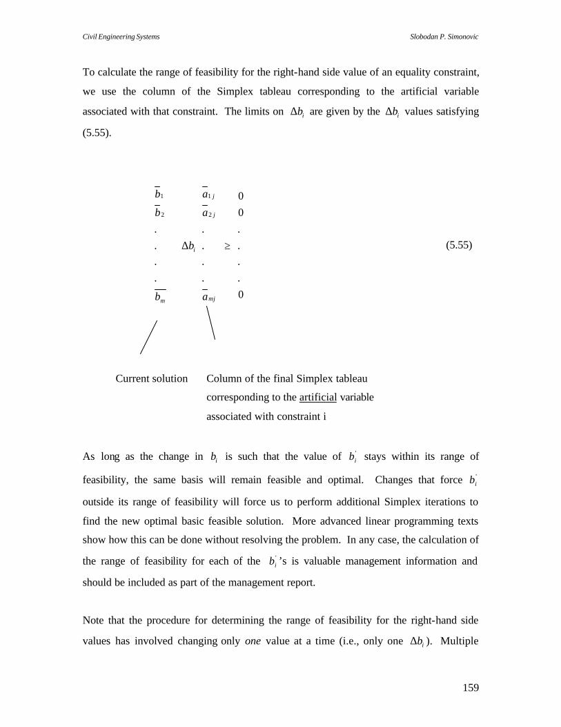
Civil Engineering Systems Slobodan P. Simonovic
159
To calculate the range of feasibility for the right-hand side value of an equality constraint,
we use the column of the Simplex tableau corresponding to the artificial variable
associated with that constraint. The limits on ib∆ are given by the ib∆ values satisfying
(5.55).
≥
∆+
0....00
.
.
.
.
.
.
.
.2
1
2
1
mj
j
j
i
m a
a
a
b
b
b
b
(5.55)
Current solution Column of the final Simplex tableau
corresponding to the artificial variable
associated with constraint i
As long as the change in ib is such that the value of 'ib stays within its range of
feasibility, the same basis will remain feasible and optimal. Changes that force 'ib
outside its range of feasibility will force us to perform additional Simplex iterations to
find the new optimal basic feasible solution. More advanced linear programming texts
show how this can be done without resolving the problem. In any case, the calculation of
the range of feasibility for each of the 'ib ’s is valuable management information and
should be included as part of the management report.
Note that the procedure for determining the range of feasibility for the right-hand side
values has involved changing only one value at a time (i.e., only one ib∆ ). Multiple

Civil Engineering Systems Slobodan P. Simonovic
160
changes are more difficult to analyze and in practice usually require the complete
generation of a new final Simplex tableau.
5.7.3 Sensitivity Analysis – The A Matrix
A change in one of the coefficients of the A matrix can have a significant effect on the
optimal solution to a linear programming problem. A complete discussion of the
ramifications of making changes in the A matrix is beyond the scope of this text.
5.8 Summary LP
Postulates
(a) Objective function and constraints can be expressed as simple algebraic expressions.
(b) Objective function must be convex and the constraints must form a convex policy
space.
(c) All decision variables must be positive.
Advantages and limitations
(1) Uses standard programs.
(2) User does not have to know details of method, only its philosophy and limitations.
(3) Can handle a large number of state variables.
(4) Can handle fewer decision variables than other programming techniques (for
example dynamic programming) on a sequential basis, but can handle a large
dimension of decision variables for one time period. (Dynamic programming must
keep the dimensionality of decision variables as small as possible, preferably less
than two within each unit time period.)
(5) Constraints tend to increase the computational cost.
(6) Requires convex systems (convex policy space).
(7) Requires linear relationships (nonlinear relationship can be linearized in several
presently available packages).
(8) Optimum obtained is only a single set of decisions (nothing known about second or
third best).

Civil Engineering Systems Slobodan P. Simonovic
161
5.9 Use of Microsoft Excel Solver for solving linear programming problems
Following material is modified from the Microsoft Excel Tutorial.
Quick Tour of Microsoft Excel Solver
Month Q1 Q2 Q3 Q4 Total Seasonality 0.9 1.1 0.8 1.2 Units Sold 3,592 4,390 3,192 4,789 15,962 Sales Revenue $143,662 $175,587 $127,700 $191,549 $638,498 Color Coding Cost of Sales 89,789 109,742 79,812 119,718 399,061 Gross Margin 53,873 65,845 47,887 71,831 239,437 Target cell Salesforce 8,000 8,000 9,000 9,000 34,000 Changing cellsAdvertising 10,000 10,000 10,000 10,000 40,000 Corp Overhead 21,549 26,338 19,155 28,732 95,775 ConstraintsTotal Costs 39,549 44,338 38,155 47,732 169,775 Prod. Profit $14,324 $21,507 $9,732 $24,099 $69,662 Profit Margin 10% 12% 8% 13% 11%
Product Price $40.00 Product Cost $25.00
The following examples show you how to work with the model above to solve for one value or several values to maximize or minimize another value, enter and change constraints, and save a problem model.
Row Contains Explanation 3 Fixed values Seasonality factor: sales are higher in quarters 2 and 4, and lower in quarters 1 and 3.
5 =35*B3*(B11+3000)^0.5 Forecast for units sold each quarter: row 3 contains
the seasonality factor; row 11 contains the cost of advertising.
6 =B5*$B$18 Sales revenue: forecast for units sold (row 5) times price (cell B18).
7 =B5*$B$19 Cost of sales: forecast for units sold (row 5) times product cost (cell B19).
8 =B6-B7 Gross margin: sales revenues (row 6) minus cost of

Civil Engineering Systems Slobodan P. Simonovic
162
sales (row 7).
10 Fixed values Sales personnel expenses.
11 Fixed values Advertising budget (about 6.3% of sales).
12 =0.15*B6 Corporate overhead expenses: sales revenues (row 6) times 15%.
13 =SUM(B10:B12) Total costs: sales personnel expenses (row 10) plus advertising (row 11) plus overhead (row 12).
15 =B8-B13 Product profit: gross margin (row 8) minus total costs (row 13).
16 =B15/B6 Profit margin: profit (row 15) divided by sales revenue (row 6).
18 Fixed values Product price.
19 Fixed values Product cost. This is a typical marketing model that shows sales rising from a base figure (perhaps due to the sales personnel) along with increases in advertising, but with diminishing returns. For example, the first $5,000 of advertising in Q1 yields about 1,092 incremental units sold, but the next $5,000 yields only about 775 units more. You can use Solver to find out whether the advertising budget is too low, and whether advertising should be allocated differently over time to take advantage of the changing seasonality factor. Solving for a Value to Maximize Another Value One way you can use Solver is to determine the maximum value of a cell by changing another cell. The two cells must be related through the formulas on the worksheet. If they are not, changing the value in one cell will not change the value in the other cell. For example, in the sample worksheet, you want to know how much you need to spend on advertising to generate the maximum profit for the first quarter. You are interested in maximizing profit by changing advertising expenditures.
nOn the Tools menu, click Solver. In the Set target cell box, type b15 or select cell B15 (first-quarter profits) on the worksheet. Select the Max option. In the By changing cells box, type b11 or select cell B11 (first-quarter advertising) on the worksheet. Click Solve. You will see messages in the status bar as the problem is set up and Solver starts working. After a moment, you'll see a message that Solver has found a solution. Solver finds that Q1 advertising of $17,093 yields the maximum profit $15,093.
nAfter you examine the results, select Restore original values and click OK to discard the results and return cell B11 to its former value. Resetting the Solver Options If you want to return the options in the Solver Parameters dialog box to their original settings so that you can start a new problem, you can click Reset All.

Civil Engineering Systems Slobodan P. Simonovic
163
Solving for a Value by Changing Several Values You can also use Solver to solve for several values at once to maximize or minimize another value. For example, you can solve for the advertising budget for each quarter that will result in the best profits for the entire year. Because the seasonality factor in row 3 enters into the calculation of unit sales in row 5 as a multiplier, it seems logical that you should spend more of your advertising budget in Q4 when the sales response is highest, and less in Q3 when the sales response is lowest. Use Solver to determine the best quarterly allocation.
nOn the Tools menu, click Solver. In the Set target cell box, type f15 or select cell F15 (total profits for the year) on the worksheet. Make sure the Max option is selected. In the By changing cells box, type b11:e11 or select cells B11:E11 (the advertising budget for each of the four quarters) on the worksheet. Click Solve.
nAfter you examine the results, click Restore original values and click OK to discard the results and return all cells to their former values. You've just asked Solver to solve a moderately complex nonlinear optimization problem; that is, to find values for the four unknowns in cells B11 through E11 that will maximize profits. (This is a nonlinear problem because of the exponentiation that occurs in the formulas in row 5). The results of this unconstrained optimization show that you can increase profits for the year to $79,706 if you spend $89,706 in advertising for the full year. However, most realistic modeling problems have limiting factors that you will want to apply to certain values. These constraints may be applied to the target cell, the changing cells, or any other value that is related to the formulas in these cells. Adding a Constraint So far, the budget recovers the advertising cost and generates additional profit, but you're reaching a point of diminishing returns. Because you can never be sure that your model of sales response to advertising will be valid next year (especially at greatly increased spending levels), it doesn't seem prudent to allow unrestricted spending on advertising. Suppose you want to maintain your original advertising budget of $40,000. Add the constraint to the problem that limits the sum of advertising during the four quarters to $40,000.
nOn the Tools menu, click Solver, and then click Add. The Add Constraint dialog box appears. In the Cell reference box, type f11 or select cell F11 (advertising total) on the worksheet. Cell F11 must be less than or equal to $40,000. The relationship in the Constraint box is <= (less than or equal to) by default, so you don't have to change it. In the box next to the relationship, type 40000. Click OK, and then click Solve.
nAfter you examine the results, click Restore original values and then click OK to discard the results and return the cells to their former values. The solution found by Solver allocates amounts ranging from $5,117 in Q3 to $15,263 in Q4. Total Profit has increased from $69,662 in the original budget to $71,447, without any increase in the advertising budget. Changing a Constraint When you use Microsoft Excel Solver, you can experiment with slightly different parameters to decide the best solution to a problem. For example, you can change a constraint to see whether the results

Civil Engineering Systems Slobodan P. Simonovic
164
are better or worse than before. In the sample worksheet, try changing the constraint on advertising dollars to $50,000 to see what that does to total profits.
nOn the Tools menu, click Solver. The constraint, $F$11<=40000, should already be selected in the Subject to the constraints box. Click Change. In the Constraint box, change 40000 to 50000. Click OK, and then click Solve. Click Keep solver solution and then click OK to keep the results that are displayed on the worksheet. Solver finds an optimal solution that yields a total profit of $74,817. That's an improvement of $3,370 over the last figure of $71,447. In most firms, it's not too difficult to justify an incremental investment of $10,000 that yields an additional $3,370 in profit, or a 33.7% return on investment. This solution also results in profits of $4,889 less than the unconstrained result, but you spend $39,706 less to get there. Saving a Problem Model When you click Save on the File menu, the last selections you made in the Solver Parameters dialog box are attached to the worksheet and retained when you save the workbook. However, you can define more than one problem for a worksheet by saving them individually using Save Model in the Solver Options dialog box. Each problem model consists of cells and constraints that you entered in the Solver Parameters dialog box. When you click Save Model, the Save Model dialog box appears with a default selection, based on the active cell, as the area for saving the model. The suggested range includes a cell for each constraint plus three additional cells. Make sure that this cell range is an empty range on the worksheet.
nOn the Tools menu, click Solver, and then click Options. Click Save Model . In the Select model area box, type h15:h18 or select cells H15:H18 on the worksheet. Click OK. Note You can also enter a reference to a single cell in the Select model area box. Solver will use this reference as the upper-left corner of the range into which it will copy the problem specifications. To load these problem specifications later, click Load Model on the Solver Options dialog box, type h15:h18 in the Model area box or select cells H15:H18 on the sample worksheet, and then click OK. Solver displays a message asking if you want to reset the current Solver option settings with the settings for the model you are loading. Click OK to proceed.
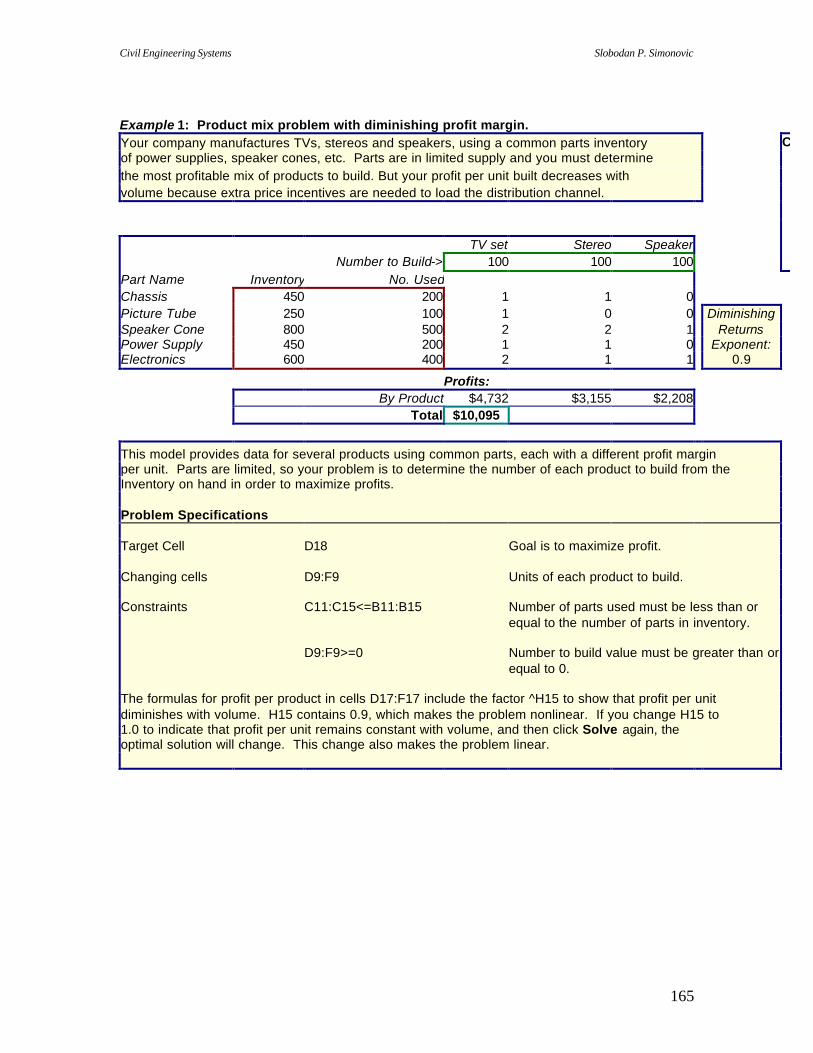
Civil Engineering Systems Slobodan P. Simonovic
165
Example 1: Product mix problem with diminishing profit margin. Your company manufactures TVs, stereos and speakers, using a common parts inventory Color Codingof power supplies, speaker cones, etc. Parts are in limited supply and you must determine the most profitable mix of products to build. But your profit per unit built decreases with volume because extra price incentives are needed to load the distribution channel. TV set Stereo Speaker Number to Build-> 100 100 100 Part Name Inventory No. Used Chassis 450 200 1 1 0 Picture Tube 250 100 1 0 0 Diminishing Speaker Cone 800 500 2 2 1 Returns Power Supply 450 200 1 1 0 Exponent: Electronics 600 400 2 1 1 0.9
Profits: By Product $4,732 $3,155 $2,208 Total $10,095
This model provides data for several products using common parts, each with a different profit margin per unit. Parts are limited, so your problem is to determine the number of each product to build from the Inventory on hand in order to maximize profits. Problem Specifications Target Cell D18 Goal is to maximize profit. Changing cells D9:F9 Units of each product to build. Constraints C11:C15<=B11:B15 Number of parts used must be less than or equal to the number of parts in inventory. D9:F9>=0 Number to build value must be greater than or equal to 0. The formulas for profit per product in cells D17:F17 include the factor ^H15 to show that profit per unit diminishes with volume. H15 contains 0.9, which makes the problem nonlinear. If you change H15 to 1.0 to indicate that profit per unit remains constant with volume, and then click Solve again, the optimal solution will change. This change also makes the problem linear.

Civil Engineering Systems Slobodan P. Simonovic
166
Example 2: Transportation Problem. Minimize the costs of shipping goods from production plants to warehouses near metropolitan demand centers, while not exceeding the supply available from each plant and meeting the demand from each metropolitan area. Number to ship from plant x to warehouse y (at intersection): Plants: Total San Fran Denver Chicago Dallas New York S. Carolina 5 1 1 1 1 1 Tennessee 5 1 1 1 1 1 Arizona 5 1 1 1 1 1 --- --- --- --- --- Totals: 3 3 3 3 3 Demands by Whse --> 180 80 200 160 220 Plants: Supply Shipping costs from plant x to warehouse y (at intersection): S. Carolina 310 10 8 6 5 4 Tennessee 260 6 5 4 3 6 Arizona 280 3 4 5 5 9 Shipping: $83 $19 $17 $15 $13 $19
The problem presented in this model involves the shipment of goods from three plants to five regional warehouses. Goods can be shipped from any plant to any warehouse, but it obviously costs more to ship goods over long distances than over short distances. The problem is to determine the amounts to ship from each plant to each warehouse at minimum shipping cost in order to meet the regional demand, while not exceeding the plant supplies. Problem Specifications Target cell B20 Goal is to minimize total shipping cost. Changing cells C8:G10 Amount to ship from each plant to each warehouse. Constraints B8:B10<=B16:B18 Total shipped must be less than or equal to supply at plant. C12:G12>=C14:G14 Totals shipped to warehouses must be greater than or equal to demand at warehouses. C8:G10>=0 Number to ship must be greater than or equal to 0. You can solve this problem faster by selecting the Assume linear model check box in the Solver Options dialog box before clicking Solve. A problem of this type has an optimum solution at which Amounts to ship are integers, if all of the supply and demand constraints are integers.

Civil Engineering Systems Slobodan P. Simonovic
167
5.10 Problems
5.1 A concrete products manufacturer makes two types of building blocks: type A and type
B. For each set of 100 type A blocks the manufacturer can make a profit of $5 whereas for
each set of 100 type B blocks he can make $8. Assume that all blocks which are produced
can be sold. It takes 1 hour to make 100 type A blocks and 3 hours to make 100 type B
blocks. Each day there are 12 hours available for block manufacturing. A set of 100 type A
blocks requires 2 units of cement, 3 units of fine aggregate , and 4 units of coarse
aggregate; a set of 100 type B blocks requires 1 unit of cement and 6 units of coarse
aggregate. Each day, 18 units of cement and 24 units of coarse aggregate are available for
block manufacturing. There is no restriction on the availability of fine aggregate. How
many type A and type B blocks should be made during the day to maximize profits?
(a) Formulate the problem as a LP problem.
(b) Name decision variables, objective function, and constraints.
(c) Solve the problem graphically.
(d) Use Excel Solver to solve the problem.
5.2 Draw the feasible region for the following LP problem:
5x1 + 5x2 = 50
x2 = 6
x1 = 8
2x1 + 4x2 = 28
x1 + 2x2 = 14
(a) Provide the extreme points.
(b) Is the feasible region convex?
(c) Indicate any redundant constraints if any.
(d) Introduce a new set of constraints that will make the feasible region infeasible.
(e) Introduce a new constraint that can make the feasible region unbounded (assuming
the objective is to maximize the objective function).

Civil Engineering Systems Slobodan P. Simonovic
168
5. 2 The Sunnyflush Company has two plants located along a stream. Plant 1 is generating
20 units of pollutants daily and plant 2 14 units. Before the wastes are discharged into the
river, part of these pollutants are removed by a waste treatment facility in each plant. The
costs associated with removing a unit of pollutant are $1,000 and $800 for plants 1 and 2.
The rates of flow in the streams are Q1 =5mgd and Q2 =2mgd, and the flows contain no
pollutants until they pass the plants. Stream standards require that the number of units of
pollutants per million gallons of flow should not exceed 2. 20% of the pollutants entering
the stream at plant 1 will be removed by natural processes before they reach plant 2. The
company wants to determine the most economical operation of its waste treatment facilities
that will allow it to satisfy the stream standards.
(a) Formulate the problem as LP problem.
(b) Name decision variables, objective function, and constraints.
(c) Solve the problem graphically.
(d) Use Excel Solver to solve the problem.
5.3 Consider the following LP problem
maximize x1 + x2
subject to
-x1 + x2 = -1
x1 - x2 = -1
Plant 1
Plant 2
Q1
Q2
Civil Engineering Systems Slobodan P. Simonovic
169
x1 = 0 and x2 =0.
(a) Find graphically the solution of the stated problem.
(b) Discuss the solution obtained in details.
(c) Modify the problem by changing the sign of both inequalities and adding one
more constraint:
x1 + x2 =6
and solve it using the Excel Solver.
5.4 The reservoir A is used for recreation (swimming, water skiing, canoeing). It is
important to keep the average depth of this reservoir within prescribed limits, which vary
from one month to the next. The engineers responsible for the operations of reservoir A
have estimated a rapid rate of seepage and evaporation from the reservoir. Since
rainfall is negligible, reservoir A must be maintained by spillage from reservoir B.
Suppose that planning horizon is 20 months. During month t, let xt denote the average
depth of the reservoir A prior to augmenting with the water from reservoir B; x1 = 25 for
month 1. Let yt be number of meters to be added to the average depth in month t (positive
value for yt indicates a decision to augment the reservoir A). Let Lt and Ut represent the
lower and upper prescribed limits, respectively, of the average reservoir depth after
augmentation in month t. Assume that xt+1 is 0.75 of the average reservoir depth in
month t after augmentat ion.
Suppose that the cost of augmenting the reservoir is ct per meter in month t. Formulate
an appropriate optimization model. Do not solve the problem.
5.5 Formulate the following linear program using the Big-M method and solve it using
Excel Solver:

Civil Engineering Systems Slobodan P. Simonovic
170
Max 4x1 + x2
subject to
2x1 + 3x2 = 4
3x1 + 6x2 = 9
x1, x2 = 0.
5.6 Consider the linear programming problem described in the Figure below:
(a) How many constraints are there?
(b) Which are binding constraints? Which are redundant?
(c) How many variables are there? What are they?
(d) At point A, which variables are greater than 0?
(e) At point A, which variables are basic? Which are non-basic?
(f) At point B, which variables are greater than 0?
(g) At point B, how many basic feasible solutions are there? What are the basic
variables associated with each basic feasible solution?
G
Constraint 4
D
Constraint 1
X2
X3 Constraint 2
Constraint 3
F
B
A
E

Civil Engineering Systems Slobodan P. Simonovic
171
5.11 References
De Neufville, R., (1990), Applied Systems Analysis: Engineering Planning and
Technology Management, McGraw Hill, New York, USA.
Hillier, F.S. and G.J. Lieberman, (1990), Introduction to Mathematical Programming,
McGraw Hill, New York, USA.
Jewell, T.K., (1986), A Systems Approach to Civil Engineering Planning and Design,
Harper and Row, New York, USA.
Civil Engineering Systems Slobodan P. Simonovic
172
6. MULTI-OBJECTIVE ANALYSIS
From the previous sections we see that the single-objective programming problem consists
of optimising one objective subject to a constraint set. On the other hand, a multiobjective
programming problem is characterised by a p-dimensional vector of objective functions:
Z(x) = [Z1(x), Z2(x), ..., Zp(x)] (6.1)
subject to:
x ∈ X
where X is a feasible region:
X = {x: x ∈ Rn, gi(x) ≤ 0, xj ≥ 0 ∀ i, j} (6.2)
where R = set of real numbers;
gi(x) = set of constraints; and
x = set of decision variables.
The word "optimization" has been purposely kept out of the definition of a multiobjective
programming problem since one can not, in general, optimise a priori a vector of objective
functions. The first step of the multiobjective problem consists of identifying the set of
nondominated solutions within the feasible region X. So instead of seeking a single optimal
solution, a set of "noninferior" solutions is sought.
6.1 Basic concepts of multiobjective analysis
The essential difficulty with multiobjective analysis is that the meaning of the optimum is
not defined so long as we deal with multiple objectives that are truly different. For example,
suppose we are trying to determine the best design of a system of dams on a river, with the
objectives of promoting "national income," reducing "deaths by flooding," and increasing

Civil Engineering Systems Slobodan P. Simonovic
173
"employment." Some designs will be more profitable, but less effective at reducing deaths.
How can we state which is better when the objectives are so different, and measured in such
different terms? How can one state with any accuracy what the relative value of a life is in
terms of national income? If one resolved that question, then how would one determine the
relative value of new jobs and other objectives? The answer is, with extreme difficulty. The
attempts to set values on these objectives are, in fact, most controversial.
To obtain a single global optimum over all objectives requires that we either establish or
impose some means of specifying the value of each of the different objectives. If all
objectives can indeed be valued on a common basis, the optimization can be stated in terms
of that single value. The multiobjective problem has then disappeared and the optimization
proceeds relatively smoothly in terms of a single- objective.
In practice it is frequently awkward if not indefensible to give every objective a relative
value. The relative worth of profits, lives lost, the environment, and other such objectives
are unlikely to be established easily by anyone, or to be accepted by all concerned. One
cannot hope, then, to be able to determine an acceptable optimum analytically.
The focus of multiobjective analysis in practice is to sort out the mass of clearly dominated
solutions, rather than determine the single best design. The result is the identification of the
small subset of feasible solutions that are worthy of further consideration. Formally, this
result is known as the set of nondominated solutions.
Nondominated solutions
To understand the concept of nondominated solutions, it is necessary to look closely at the
multiobjective problem (6.1) and (6.2). (Note: The nondominated solutions are sometimes
referred to by other names: noninferior, Pareto optimal, efficient, etc. Throughout this text
different names will be used with the same meaning.)
The essential feature of the multiobjective problem is that the feasible region of production
of the solutions is much more complex than for a single-objective. In single optimization,
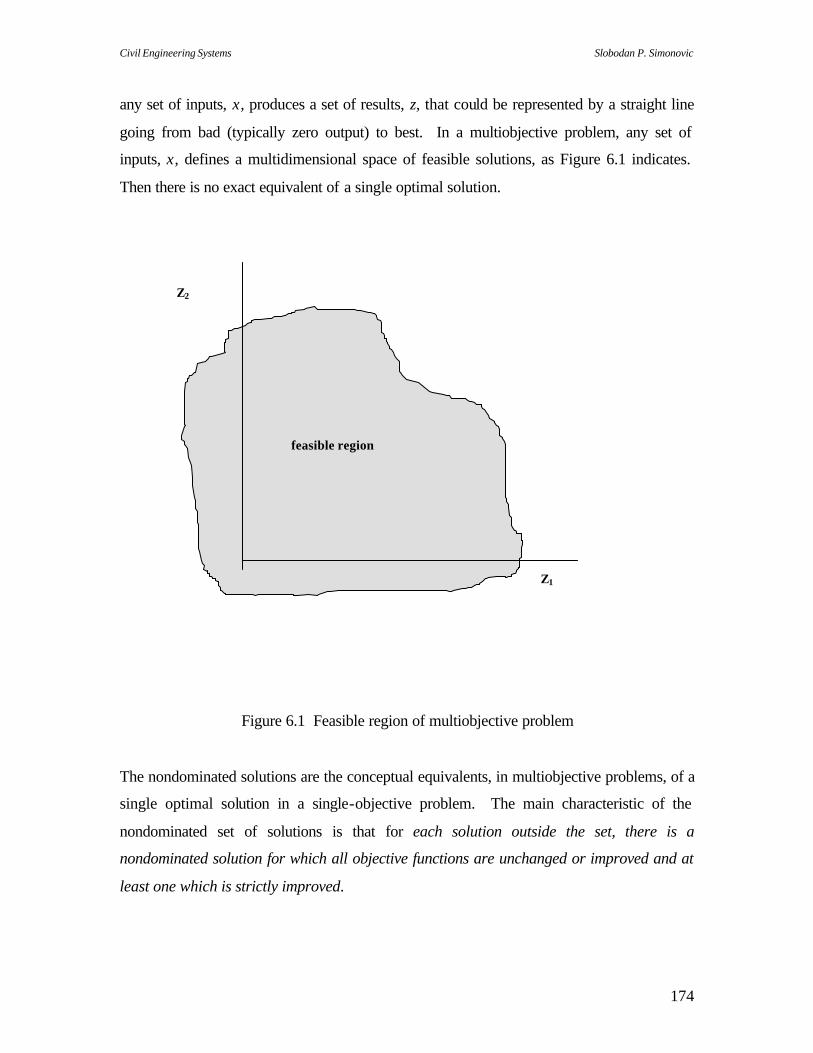
Civil Engineering Systems Slobodan P. Simonovic
174
any set of inputs, x, produces a set of results, z, that could be represented by a straight line
going from bad (typically zero output) to best. In a multiobjective problem, any set of
inputs, x, defines a multidimensional space of feasible solutions, as Figure 6.1 indicates.
Then there is no exact equivalent of a single optimal solution.
Figure 6.1 Feasible region of multiobjective problem
The nondominated solutions are the conceptual equivalents, in multiobjective problems, of a
single optimal solution in a single-objective problem. The main characteristic of the
nondominated set of solutions is that for each solution outside the set, there is a
nondominated solution for which all objective functions are unchanged or improved and at
least one which is strictly improved.
Z1
Z2
feasible region

Civil Engineering Systems Slobodan P. Simonovic
175
The preferred design for any problem should be one of the nondominated solutions. So long
as all objectives worth taking into account have been considered, no design that is not
among the nondominated solutions is worthwhile: it is dominated by some designs that are
preferable on all accounts. This is the reason multiobjective analysis focuses on the
determination of the nondominated solutions.
It is often useful to group the noninferior solutions into major categories. The purpose of
this exercise is to facilitate discussions about which solution to select. Indeed, to the extent
that it is not possible to specify acceptable relative values for the objectives, and thus
impossible to define the best design analytically, it is necessary for the choice of the design
to rest on judgement. As individuals find it difficult to consider a large number of
possibilities, it is helpful to focus attention on major categories.
If we introduce the levels of acceptability for each of the objectives the nondominated
solutions are best divided into two types of categories: the major alternatives and the
compromises. A major alternative group of dominated solutions represents the best
performance on some major objective. As Figure 6.2 ind icates, the major alternatives
represent polar extremes. A compromise group lies somewhere in between the major
alternatives.
The remainder of the feasible region of solutions is likewise usefully categorised into
dominated and excluded solutions. Dominated solutions are those that are inferior in all
essential aspects to the other solutions. They can thus be set aside from further
consideration. Excluded solutions are those that perform so badly on one or more
dimensions that they lie beneath the threshold of acceptability. Thus, they may be dropped
from further consideration.
The concepts of nondominated solutions and of major categories are often highly useful in a
practical sense. They organise the feasible designs into a small number of manageable ideas
and draw attention to the choices that must be made. These ideas can be applied even when
the feasible region is not defined analytically.
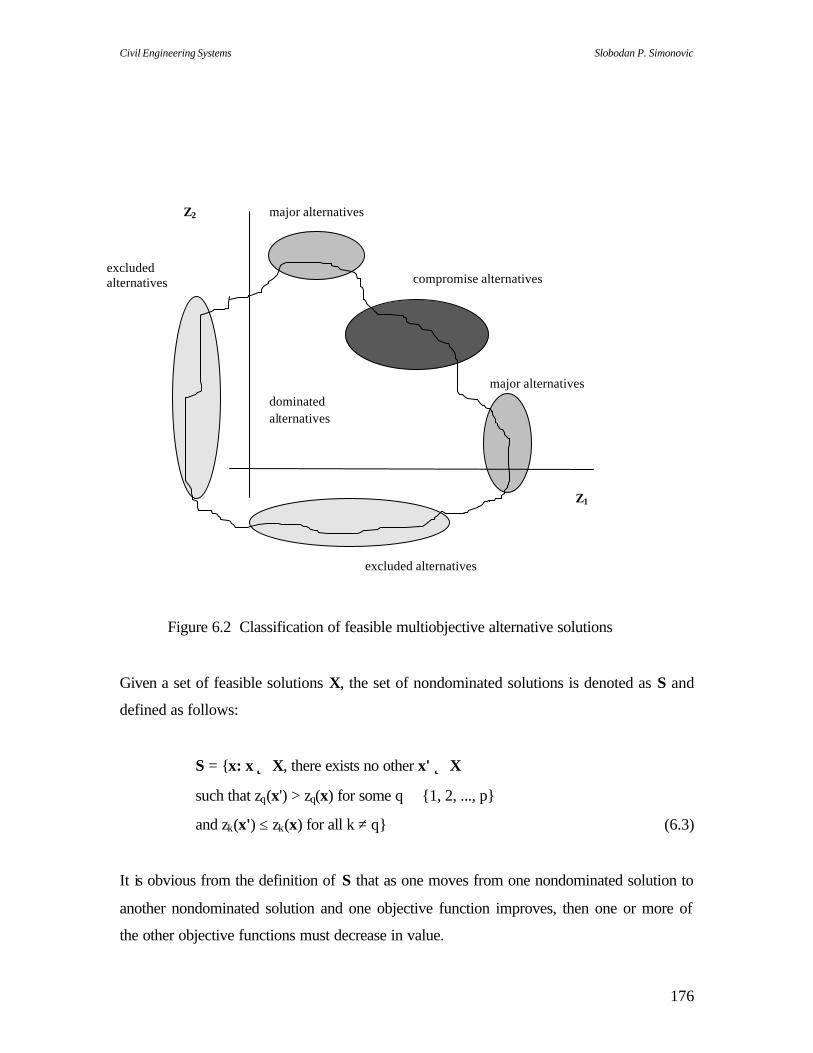
Civil Engineering Systems Slobodan P. Simonovic
176
Figure 6.2 Classification of feasible multiobjective alternative solutions
Given a set of feasible solutions X, the set of nondominated solutions is denoted as S and
defined as follows:
S = {x: x ∈ X, there exists no other x' ∈ X
such that zq(x') > zq(x) for some q ∈ {1, 2, ..., p}
and zk(x') ≤ zk(x) for all k ≠ q} (6.3)
It is obvious from the definition of S that as one moves from one nondominated solution to
another nondominated solution and one objective function improves, then one or more of
the other objective functions must decrease in value.
Z1
Z2 major alternatives
compromise alternatives
major alternatives dominated alternatives
excluded alternatives
excluded alternatives

Civil Engineering Systems Slobodan P. Simonovic
177
Classification of multiobjective techniques
Multiobjective techniques are classified into three groups: (a) methods for generating the
nondominated set; (b) methods with prior articulation of preferences; and (c) methods with
progressive articulation of preferences.
(a) Methods for generating the nondominated set. A generating method does just one thing
- it considers a vector of objective functions and uses this vector to identify and generate the
subset of nondominated solutions in the initial feasible region. In doing so, these methods
deal strictly with the physical realities of the problem (i.e. the set of constraints) and make
no attempt to consider the preferences of a decision maker (DM). The desired outcome,
then, is the identification of the set of nondominated solutions to help the DM gain insight
into the physical realities of the problem at hand.
There are several methods available to generate the set of nondominated solutions, and four
of these methods are widely known. These methods are:
· Weighting method;
· ε-constraint method;
· Phillip's linear multiobjective method; and
· Zeleny's linear multiobjective method.
The first two methods transform the multiobjective problem into a single-objective
programming format and then, by parametric variation of the parameters used to effect the
transformation, the set of nondominated solutions can be generated. The weighting and
constraint methods can be used to obtain nondominated solutions when the objective
functions and/or constraints are nonlinear.
The last two methods generate the nondominated set for linear models only. However, these
two approaches do not require the transformation of the problem into a single-objective
programming format. These methods operate directly on the vector of objectives to obtain
the nondominated solutions.
Civil Engineering Systems Slobodan P. Simonovic
178
Further insight into the weighting method will be presented in one of the following sections
of this document.
(b) Methods with prior articulation of preferences. Methods in this class are further divided
into continuous and discrete methods.
Continuous. Once the set of nondominated solutions for a multiobjective problem have
been identified using any of the methods mentioned in (a), the decision maker (DM) is able
to select one of those nondominated solutions as his final choice. Then, this solution is one
that meets the physical constraints of the problem and happens to satisfy the value structure
of the DM as well. However, more likely is the situation where the DM is unwilling or
unable to "settle down" for one of those solutions made available to him and would like to
voice his preferences regarding the various objective functions in the search for that choice
solution. Various methods are available where the DM is asked to articulate his worth or
preference structure, and these preferences are then built into the formulation of the
mathematical model for the multiobjective problem.
To assist the DM in articulating his/her preferences, a series of questions may be put to
him/her where he/she is asked to consider specific tradeoffs among several objectives and
elicit a preference for a particular allocation for each objective. In the process, use is made
of basic elements of utility theory and probability.
The net effect of articulating the preferences of the DM prior to solving the multiobjective
problem is to reduce the set of nondominated solutions to a much smaller set of solutions,
facilitating the task of selecting a final choice. Depending on the method used, this smaller
set may contain several solutions, one solution, or none at all. Preferences, then, provide an
ordering of solutions stronger than that provided by the concept of nondominated solutions.
The most known methods in the group of continuous methods with prior articulation of
preferences are:
· Goal programming;
· Utility function assessment; and
Civil Engineering Systems Slobodan P. Simonovic
179
· The surrogate worth tradeoff method.
Discrete. There are many decision situations in which the DM must choose among a finite
number of alternatives which are evaluated on a common set of noncommensurable multiple
objectives or criteria. Problems of this sort occur in many practical situations, for example,
which one of five candidates should be hired, which of ten suppliers of an important
component should be selected, which of eight systems should be chosen and implemented,
etc.
In problems of the above type, the solution process can be described as follows. First, a
statement of the general goals relating to the situation is made. Second, the alternatives
must be identified or developed. Third, the common set of relevant criteria for evaluation
purposes must be specified. Fourth, the levels of the criteria for each alternative must be
determined. Finally, a choice based on a formal or informal evaluation procedure is made.
The structure of the discrete problem can be represented in a payoff matrix as shown in
Table 6.1. The rating of the ith objective on the jth alternative (i = 1, 2, ..., m and j = 1, 2, ...,
n) is represented by rij.
Clearly the problem of choice in a problem such as that depicted by Table 6.1 is sufficiently
complex as to require some type of formal assistance. Determining the worth of the
alternatives that vary on many dimensions presents formidable cognitive difficulties. People
faced with such complex decisions react by reducing the task complexity by using various
heuristics. Unfortunately, it has been observed that decision makers who rely on heuristic
decision rules systematically violate the expected utility principle. Moreover, decision
makers tend to ignore many relevant variables in order to simplify their problem to a scale
consistent with the limitations of the human intellect. While such simplification facilitates
the actual decision making, it can clearly result in suboptimal behaviour.
In effect, as the decision-making task increases, researchers have observed systematic
discrepancies between rational theory and actual behaviour. Evidence exists that even

Civil Engineering Systems Slobodan P. Simonovic
180
experts have great difficulty in intuitively combining information in appropriate ways. In
fact, these studies and many others indicate that global judgements (i.e., combinations of
attributes) are not nearly as accurate as analytical combinations. Due to severe limitations of
the intuitive decision-making process, it is evident that analytical methods are needed to
help determine the worth of multiattributed alternatives.
Table 6.1 Payoff matrix
Alternatives 1 2 ... n
Criteria 1 r11 r12 ... r1n
2 r21 r22 ... r2n
...
...
m rm1 rm2 ... rmn
Ideally, the alternative which maximises the utility of the DM should be chosen. Therefore,
the obvious first step in the application of any discrete multiattributed method is the
elimination of all dominated alternatives. Occasionally, for discrete problems, this
dominance analysis will yield only one nondominated alternative, in which case the problem
is solved; no further analysis is needed.
The methods available in this group range from the very simple to the very complex. Some
of the methods are:
· Exclusionary screening;
· Conjunctive ranking;
· Weighted average;
· ELECTRE I and II;
· Indifference tradeoff method;

Civil Engineering Systems Slobodan P. Simonovic
181
· Direct-rating method; etc.
(c) Methods of progressive articulation of preferences. The characteristic of the methods in
this group is the following general algorithmic approach. First, a nondominated solution is
identified. Second, the decision maker (DM) is solicited for tradeoff information concerning
this solution, and the problem is modified accordingly. These two steps are repeated until
the DM indicates acceptability of a current achievement level, provided one exists.
The methods typically require greater DM involvement in the solution process. This has the
advantage of allowing the DM to gain a greater understanding and feel for the structure of
the problem. On the other hand, the required interaction has the disadvantage of being time-
consuming. The DM may not feel that the investment of the time required provides any
better decision making than ad hoc approaches. That is, the DM may perceive the costs to
be greater than any benefits. In fact, Cohon and Marks (1975) point out that decision
makers have less confidence in the interactive algorithms and find them more difficult to use
and understand than the trial and error methods. Certainly, one can not ignore these
behavioural difficulties. What they seem to indicate is that more research is needed on how
analysts can successfully interact with decision makers to implement improved but complex
decision aids.
At any rate, knowledge of some of the advantages and disadvantages should help the
management scientists or system analysts in choosing the appropriate decision aid.
Certainly, the use of any of the methods as aids to decision making will depend on the
analyst's assessment of the personality and tastes of the DM. The methods of progressive
articulation of preferences vary in the degree of sophistication and the degree of required
interaction. Some of them are:
· Step method (stem);
· Method of Geoffrion;
· Compromise programming;
· SEMOPS method; and others.

Civil Engineering Systems Slobodan P. Simonovic
182
6.2 Multiobjective analysis – application examples
River Basin Planning
Alternative strategies for the Santa Cruz River Basin, as proposed by the Corps of
Engineers, are examined by Gershon et al. (1980) with the methods ELECTRE I and II.
Combinations of flood control actions (e.g. levee construction, channelization, dams,
reservoirs, and flood plain management) and water supply actions (e.g. wastewater
reclamation, new groundwater development, the Central Arizona project, and conservation
measures) are combined to represent 25 alternative systems.
An adaptation of the constraint method is demonstrated by Cohon et al. (1979) in the
development of the Lehigh River Basin. Maximisation of economic efficiency and the
minimisation of reservoir capacity (as a surrogate for environmental quality) are the two
objectives considered.
Conjunctive Water Uses
Simultaneous utilisation of surface and groundwater sources is often a desirable
management alternative, particularly in urban water supply. In a case study of Western
Skane, Sweden, Hashimoto (1980) considers local groundwater and two pipeline systems to
supply five municipalities. A two-level hierarchy is structured to aid in the decision process
and the STEM method is used to obtain tradeoffs among five objectives pertaining to lake
water levels, downstream releases, and operating costs.
Multiattribute utility functions are used by Keeney and Wood (1977) to evaluate and rank
five water systems along the Tisza River Basin in Hungary.
Northeastern United States Water Supply (NEWS) Study (Corps of Engineers, July 1977) is
one of the better known studies conducted in the U.S.A. The region extends about 1,000
miles from northern Maine to southern Virginia, averaging 200 miles in width from the

Civil Engineering Systems Slobodan P. Simonovic
183
Atlantic Coast. It is significant because of the scale of the problem, the application of state-
of-the-art planning techniques, and the intense institutional analysis performed.
Reservoir Operation
In developing a plan of operation of a reservoir, primary consideration may be given to
reducing the damaging peak flood stages at principal downstream flood centres. Other
objectives may involve recreation and water quality enhancement.
Tauxe et al. (1979) have applied multiobjective dynamic programming (MODP) to the
operation of the Shasta Reservoir in California. The three objectives considered are (1)
maximisation of cumulative dump energy generated above the level of firm energy; (2)
minimisation of the cumulative evaporation or loss of the resource; and (3) maximisation of
the firm energy.
Cooperative n-person game theory is used by Fronza et al. (1977) to establish yearly
contract volumes in the operation of the Lake Maggiore reservoir in northern Italy. A
situation is described in which no "water sellers" or supervisors exist and the solution is
shown to result from a trade-off between two users.
Simonovic and Burn (1989) used multiobjective compromise programming for short-term
operation of a single multipurpose reservoir. An improved methodology for short-term
reservoir operation is derived which considers the operating horizon as a decision variable
which can change in real time. The optimal value of the operating horizon is selected based
on the trade-off between a more reliable inflow forecast for shorter horizons and better
reservoir operations associated with the use of longer operating horizons.
The methodology, based on combined use of simulation and multiobjective analysis, has
been developed by Simonovic (1991). It has been used to modify the existing operating
rules of the Shellmouth Reservoir in Manitoba, Canada. Flood control and the water supply
objectives are confronted with the use of reservoir water for dilution of the heated effluent
from a thermal generating plant and the improvement of water quality in the river.

Civil Engineering Systems Slobodan P. Simonovic
184
Flood Plain Management
Both structural and nonstructural measures can reduce flood damages. Structural means
include levees and dams to physically prevent floods from reaching an area. Nonstructural
means include (1) restrictions on the use of flood-prone areas and reduction of the runoff
produced by storms; and (2) the purchase of flood plain land that is already developed and
its conversion to flood-compatible uses to protect life and property.
Novoa and Halff (1977) evaluate eight alternative flooding remedies ranging from mono-
action to stream channelization to complete development of portions of the City of Dallas,
Texas. The method of weighted averages is used to evaluate and rank the eight alternative
plans; evaluation criteria reflect: (1) relative flood protection; (2) relative neighbourhood
improvement; (3) number of relocated families; (4) project cost; (5) maintenance cost;
and (6) legal considerations.
Water Quality Management
The public's increasing concern with water pollution demands that the attention be directed
to the analysis of water quality determinants, both physical and chemical. These
determinants can include dissolved oxygen, coliform count, temperature, and concentrations
of various pollutants.
An excellent compilation of papers in water supply and water quality has been published by
the Institute for Water Resources, U.S. Army Corps of Engineers (IWR report 81-R04, April
1981). It discusses water quality in the context of a variety of activities such as interbasin
water transfer, urban water supply, coal strip-mining, municipal reuse of wastewater,
agricultural and industrial uses. A second excellent discussion of water quality in the
context of regional planning is given by Goodman (1982). This particular book is strongly
recommended as it presents a comprehensive view of water resources planning with a
multitude of case studies.

Civil Engineering Systems Slobodan P. Simonovic
185
A regional planning framework that integrates land and water quality management models is
that developed by Das and Haimes (1979). The Surrogate Worth Tradeoff (SWT) method is
applied here to investigate tradeoffs among four planning objectives: (1) sheet erosion
control; (2) phosphorous loading; (3) biological oxygen demand; and (4) nonpoint source
pollution cost control.
In a hypothetical example based on the institutional arrangements of the Yodo River basin
of Japan, Nakayama et al. (1980) discuss a water quality control problem with three
objectives: (1) BOD concentration at the inflow point into Osake Bay; (2) treatment cost in
the upper reach (Katsura and Uji River basins); and (3) treatment cost in the lower reach
(Yodo River basin).
Brill et al. (1976) have analysed an effluent charge program for the Delaware River and
proposed metrics for a distribution objective that allows the explicit consideration of
efficiency-equity tradeoffs.
Water and Related Land Resources
Development of water resources frequently affects or relates to the development of land
resources and vice versa. Activities such as coal strip-mining, land reclamation, watershed
management, and land use planning relate closely to the hydrology of the area and the
availability of water resources (e.g. surface and groundwater).
Goicoechea et al. (1982) have applied mathematical programming to the problem of
reclaiming lands disturbed by coal strip-mining activities in the Black Mesa region of
northern Arizona. This study suggests a reclamation program to enable the land to sustain
agricultural, livestock grazing, fish pond-harvesting, and recreational uses. The
PROTRADE method is used in the process to examine levels of attainment and the trade-off
for five objectives: (1) livestock production; (2) water runoff augmentation; (3) farming of
selected crops; (4) sediment control; and (5) fish yield. This method, as noted earlier,
allows the use of random variables to represent parameters in the objective functions; to
Civil Engineering Systems Slobodan P. Simonovic
186
generate objective tradeoffs the decision maker is able to consider both the level of
attainment and the probability of attainment for each objective function.
The same authors have investigated the implementation of mechanical and chemical
vegetation treatments to promote water runoff in the San Pedro River basin, Tucson,
Arizona. The TRADE method was used to examine tradeoffs among five objectives: (1)
runoff augmentation; (2) sediment control; (3) animal wildlife balance; (4) recreation; and
(5) commercial benefits.
Gershon et al. (1981) have investigated the impact of alternative river basin development
plans using the ELECTRE I technique for screening and the ELECTRE II technique for the
final ranking. They illustrate the approach by means of the case study of the Tucson basin,
Arizona. A systems analysis of the problem leads to defining an array of 25 alternative
systems versus 13 criteria, only 5 of which are quantified. In the same study sensitivity of
the results to changes in weights and scales is investigated.
6.3 The weighting method
The weighting method belongs to the group of techniques for generating a nondominated
set. It is based on the idea of assigning weights to the various objective functions,
combining these into a single-objective function, and parametrically varying the weights to
generate the nondominated set.
Mathematically, the weighting method can be stated as follows:
max z(x) = w1z1(x) + w2z2(x) + ... + wpzp(x) (6.4)
subject to:
x ∈ X
which can be thought of as an operational form of the formulation

Civil Engineering Systems Slobodan P. Simonovic
187
max-dominate z(x) = [z1(x), z2(x) ..., zp(x)]
subject to:
x ∈ X
In other words, a multiobjective problem has been transformed into a singleobjective
optimization problem for which the solution methods exist. The coefficient wi operating on
the ith objective function, zi(x), is called a weight and can be interpreted as "the relative
weight or worth" of that objective when compared to the other objectives. If the weights of
the various objectives are interpreted as representing the relative preferences of some DM,
then the solution to (6.4) is equivalent to the best-compromise solution, that is, the optimal
solution relative to a particular preference structure. Moreover, the optimal solution to (6.4)
is a nondominated solution, provided all the weights are positive. The reasoning behind the
nonnegativity requirement is as follows. Allowing negative weights would be equivalent to
transforming the maximisation problem into a minimisation one, for which a different set of
nondominated solutions will exist. The trivial case where all the weights are zero will
simply identify every x ∈ X as an optimal solution, and will not distinguish between the
dominated and the nondominated solutions.
Conceptually, the generation of the nondominated set using the method of weights appears
simple. However, in practice the generation procedure is quite demanding. Several weight
sets can generate the same nondominated point. Furthermore, moving from one set of
weights to another set of weights may result in skipping a nondominated extreme point.
Subsequent linear combinations of the observed adjacent extreme points would, in many
cases, yield a set of points that are only "close" to the nondominated border. In other words,
in practice, it is quite possible to miss using weights that would lead to an extreme point.
Consequently, the most that should be expected from the weighting method is an
approximation of the nondominated set.

Civil Engineering Systems Slobodan P. Simonovic
188
The sufficiency of the approximation obviously relates to the proportion of the total number
of extreme points that are identified. For example, assume each weight is varied
systematically between zero and some upper limit using a predetermined step size. It seems
reasonable to believe that the choice of a large increment will result in more skipped
extreme points than the choice of a small increment. However, the smaller the increment
the greater the computational requirements. There exists a tradeoff between the accuracy of
the specification of the nondominated set and the costs of the computational requirements.
Judgement by the DM and the analyst must be exercised to determine the desired balance.
Class exercise:
A State water agency is responsible for the operation of a multipurpose reservoir used for
(a) municipal water supply; (b) groundwater recharge; and (c) the control of water quality
in the river downstream from the dam. Allocating the water to the first two purposes is,
unfortunately, in conflict with the third purpose. The agency would like to minimise the
negative effect on the water quality in the river and, at the same time, maximise the benefits
from the municipal water supply and groundwater recharge.
Thus, there are two objectives: minimise the increase in river pollution and maximise
profits. Tradeoffs between these two objectives are sought to assist the water agency in the
decision-making process. The available data is listed in Table 6.2
The following assumptions are made:
(i) One time period is involved; t = 0, 1.
(ii) Allocation is limited to two restrictions: (a) pump capacity is 8 hr per
period; and (b) labour capacity is 4 man-hours per period.

Civil Engineering Systems Slobodan P. Simonovic
189
Table 6.2 Available data for an illustrative example
Water Supply Groundwater
Recharge
Number of units of water delivered x1 x2
Number of units of water required 1.0 5.0
Pump time required (hr) 0.5 0.25
Labour time required (man-hour) 0.2 0.2
Direct water costs ($) 0.25 0.75
Direct labour costs ($) 2.75 1.25
Sales price of water per unit ($) 4.0 5.0
(iii) Total amount of water in the reservoir available for allocation is 72 units.
(iv) The pollution in the river increases by three units per unit of water used for
water supply and two units per unit of water used for groundwater recharge.
Based on the preceding information the objective functions and constraint s of the problem
can be formulated. The contribution margin (selling price/unit less variable cost/unit) of
each allocation can be calculated:
Municipal water supply
$4.00 - $0.25 - $2.75 = $1.00 per unit of water delivered
Sales Direct water Direct
price cost labour
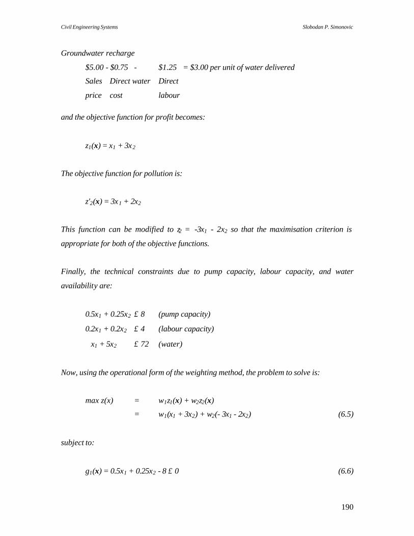
Civil Engineering Systems Slobodan P. Simonovic
190
Groundwater recharge
$5.00 - $0.75 - $1.25 = $3.00 per unit of water delivered
Sales Direct water Direct
price cost labour
and the objective function for profit becomes:
z1(x) = x1 + 3x2
The objective function for pollution is:
z'2(x) = 3x1 + 2x2
This function can be modified to z2 = -3x1 - 2x2 so that the maximisation criterion is
appropriate for both of the objective functions.
Finally, the technical constraints due to pump capacity, labour capacity, and water
availability are:
0.5x1 + 0.25x2 ≤ 8 (pump capacity)
0.2x1 + 0.2x2 ≤ 4 (labour capacity)
x1 + 5x2 ≤ 72 (water)
Now, using the operational form of the weighting method, the problem to solve is:
max z(x) = w1z1(x) + w2z2(x)
= w1(x1 + 3x2) + w2(- 3x1 - 2x2) (6.5)
subject to:
g1(x) = 0.5x1 + 0.25x2 - 8 ≤ 0 (6.6)
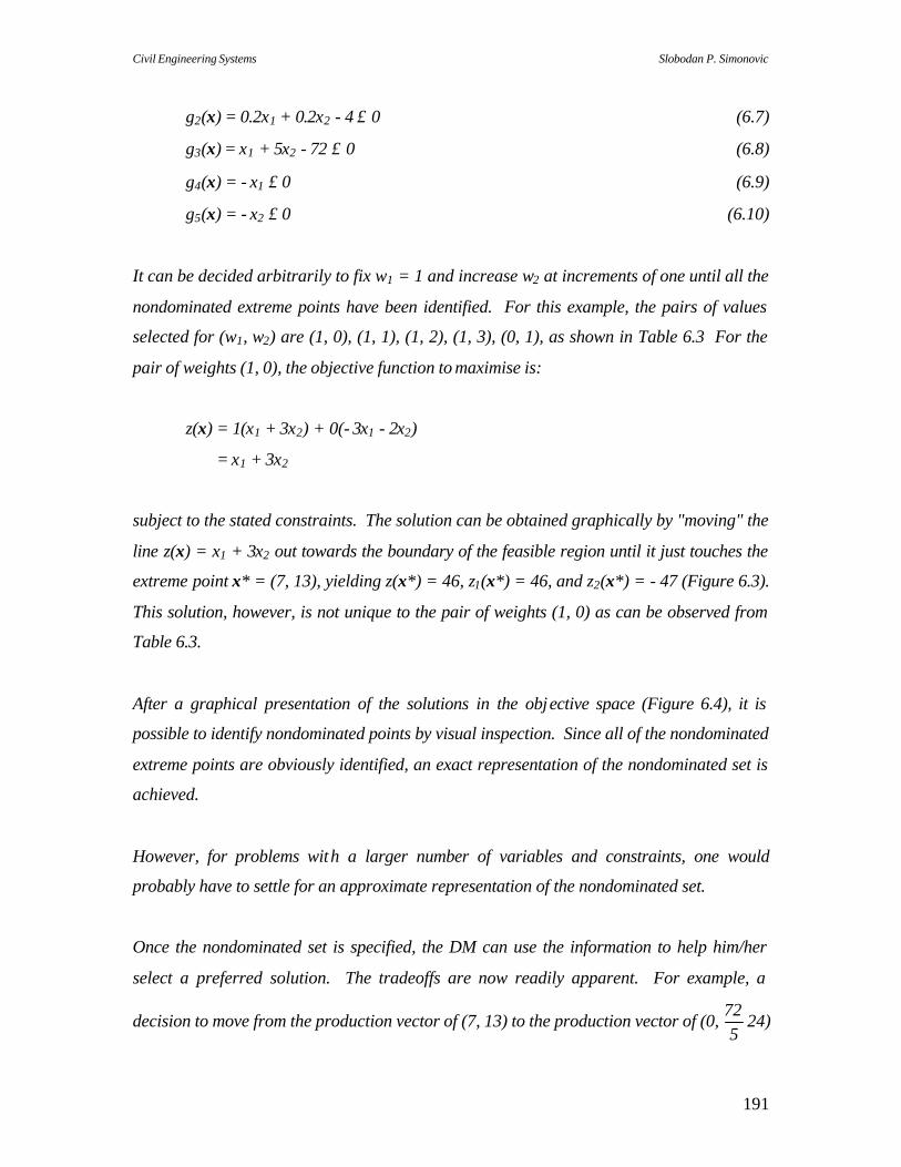
Civil Engineering Systems Slobodan P. Simonovic
191
g2(x) = 0.2x1 + 0.2x2 - 4 ≤ 0 (6.7)
g3(x) = x1 + 5x2 - 72 ≤ 0 (6.8)
g4(x) = - x1 ≤ 0 (6.9)
g5(x) = - x2 ≤ 0 (6.10)
It can be decided arbitrarily to fix w1 = 1 and increase w2 at increments of one until all the
nondominated extreme points have been identified. For this example, the pairs of values
selected for (w1, w2) are (1, 0), (1, 1), (1, 2), (1, 3), (0, 1), as shown in Table 6.3 For the
pair of weights (1, 0), the objective function to maximise is:
z(x) = 1(x1 + 3x2) + 0(- 3x1 - 2x2)
= x1 + 3x2
subject to the stated constraints. The solution can be obtained graphically by "moving" the
line z(x) = x1 + 3x2 out towards the boundary of the feasible region until it just touches the
extreme point x* = (7, 13), yielding z(x*) = 46, z1(x*) = 46, and z2(x*) = - 47 (Figure 6.3).
This solution, however, is not unique to the pair of weights (1, 0) as can be observed from
Table 6.3.
After a graphical presentation of the solutions in the objective space (Figure 6.4), it is
possible to identify nondominated points by visual inspection. Since all of the nondominated
extreme points are obviously identified, an exact representation of the nondominated set is
achieved.
However, for problems with a larger number of variables and constraints, one would
probably have to settle for an approximate representation of the nondominated set.
Once the nondominated set is specified, the DM can use the information to help him/her
select a preferred solution. The tradeoffs are now readily apparent. For example, a
decision to move from the production vector of (7, 13) to the production vector of (0, 725
24)

Civil Engineering Systems Slobodan P. Simonovic
192
results in a decrease of 2.8 units of profit with the resulting benefit of a reduction of 18.2
units
02468
10121416
0 5 10 15 20
X1
X2
Figure 6.3 Feasible region and the nondominated set in decision space
Table 6.3 Pairs of weights and associated nondominated solutions
Weights
(w1, w2)
Nondominated
Extreme Point
x* = (x1, x2)
z1(x*)
z2(x*)
z(x)
(1, 0) (7, 13) 46 - 47 46
(1, 1) (0,
725
25) 216
526 -
1445
27 725
28
(1, 2) (0, 0) 0.0 0.0 0.0
(1, 3) (0, 0) 0.0 0.0 0.0
(0, 1) (0, 0) 0.0 0.0 0.0
nondominated set

Civil Engineering Systems Slobodan P. Simonovic
193
-60
-50
-40
-30
-20
-10
0
0 10 20 30 40 50
Z1
Z2
nondominated set
Figure 6.4 Feasible region and the nondominated set in objective space
of pollution. This may be perceived as too great a sacrifice and feasible production vectors
in-between these two extremes with the corresponding tradeoffs could be examined.
6.4 Problems
6.1 A new Civil Engineering graduate has job offers from five different companies and is
faced with the problem of selecting a company within a week. The individual lists in
the form of a payoff matrix all of the important information:
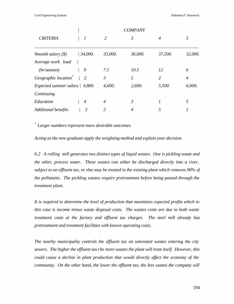
Civil Engineering Systems Slobodan P. Simonovic
194
| COMPANY
CRITERIA | 1 2 3 4 5
_________________________________________________________________________
9month salary ($) | 34,000. 33,000. 36,000. 37,500. 32,000.
Average work load |
(hr/season) | 9 7.5 10.5 12 6
Geographic location* | 2 3 5 2 4
Expected summer salary | 4,800. 4,600. 2,600. 5,500. 6,000.
Continuing
Education | 4 4 3 1 5
Additional benefits | 3 2 4 5 1
* Larger numbers represent more desirable outcomes.
Acting as the new graduate apply the weighting method and explain your decision.
6.2 A rolling mill generates two distinct types of liquid wastes. One is pickling waste and
the other, process water. These wastes can either be discharged directly into a river,
subject to an effluent tax, or else may be treated in the existing plant which removes 90% of
the pollutants. The pickling wastes require pretreatment before being passed through the
treatment plant.
It is required to determine the level of production that maximizes expected profits which in
this case is income minus waste disposal costs. The wastes costs are due to both waste
treatment costs at the factory and effluent tax charges. The steel mill already has
pretreatment and treatment facilities with known operating costs.
The nearby municipality controls the effluent tax on untreated wastes entering the city
sewers. The higher the effluent tax the more wastes the plant will treat itself. However, this
could cause a decline in plant production that would directly affect the economy of the
community. On the other hand, the lower the effluent tax, the less wastes the company will

Civil Engineering Systems Slobodan P. Simonovic
195
treat and product ion will be higher. This means the community will be subsidizing treating
the plant's waste at the city sewage plant.
Examine the problem using linear programming and solvi it using Excel Solver in order that
profits for the steel plant may be optimized according to the city's effluent charges. Apply
the Weighting Method for w=1,2 to assist the steel company in making profit projections
that reflect the city's current effluent charges and a contemplated doubling of those charges.
The following data is available:
income on steel manufactured = $25/ton
pickle wastes generated = .1 thousand gallons/ton of steel
process water generated = 1 thousand gallons/ton of steel
cost of pretreating pickle waste = $.2/thousand gallons
cost of treating process water and pretreated pickle waste = $.1/thousand gallons
pretreatment plant capacity = 2,000,000 gallons/day
treatment plant capacity = 50,000,000 gallons/day
treatment plant efficiency = .9 (both wastes)
effluent tax on untreated pickle waste = $.15/thousand gallons
effluent tax on untreated process water = $.05/thousand gallons.
The operation is shown in Figure 6.5. Also the city has imposed restrictions on how much
untreated waste can be put into the sewer. No more than 500,000 gal/day of pickle water or
10,000,000 gal/day of process water may be discharged without treatment.

Civil Engineering Systems Slobodan P. Simonovic
196
Figure 6.5 Layout of the waste facilities (after Hipel et al, 1976)
6.3 NIS consultatnts has evaluated proposed sites for a multipurpose water facility along
two objectives: economic benefits (EB) and environmental quality improvement (EQUI).
The optimal performance of each site is given by the following (EB, EQUI) pairs:
A(20,135) B(75,135) C(90,100) D(35,1050) E(82,250) F(60,-50) G(60,550) H(75,500)
I(70,620) J(10,500) K(40,350) L(30,800) N(55,250) O(40,-80) P(30,500) Q(30,900)
R(60,950) S(80,-150) T(45,550) U(25,1080) V(70,800) W(63,450).
Solve graphically.
(a) List excluded, dominated and nondominated alternative sites.
steel plant tons of steel
per day
x1
pretreatment
treatment
x2
x3
pickle waste 0.1 x1
process water 1 x1
1x1-x3 x2 +x3
0.1x1-x2
city trunk sewer

Civil Engineering Systems Slobodan P. Simonovic
197
(b) Identify nondominated solutions by maximizing EB subject to EQUI ≥ b where
b=200,400,600 and 800.
(c) Identify nondominated solution by the weighting method assigning relative
weight to (EB, EQUI) of (20,8).
6.4 Consider the multiobjective problem:
max 5x1 - 2x2 and -x1 + 4x2
subject to
-x1 + x2 <= 3
x1 + x2 <= 8
x1 <= 6
x2 <= 4
xi >= 0
(i) Graph the nondominated solutions in decision space.
(ii) Graph the nondominated combinations of the objectives in objective space.
(iii) Reformulate the problem to illustrate the weighting method for defining all
nondominated solutions of part (i) and illustrate this method in decision and objective
space.
6.5 Evaluate a plan for disposing of wastewater from a treatment plant. For the given
situation you want to use the best combination of two methods: a filetr for tertiary treatment
and irrigation with the effluent. The net benefits are: irrigation $5 per m3/s; tertiary
treatment -$2 per m3/s. Another objective is to maximize the disolved oxygen (DO) in the
river bordering the treatment plant and irrigated area. The DO will decrease by 1 mg/l for
each m3/s of effluent irrigated and increase by 4 mg/l for eaxh m3/s given tertiary treatment.
The amount of effluent filtered must be less than 3 m3/s plus the amount of effluent used for
irrigation (measured in m3/s). The total system (tertiary with irrigation) can not exceed 8
m3/s; moreover, physical constraints on the capacity of the available land limit the amount

Civil Engineering Systems Slobodan P. Simonovic
198
for irrigation to 6 m3/s and the amount of effluent for tertiary treatment to 4 m3/s. Consider
both the economic and the water quality objectives, conduct a multiobjective analysis using
the weighting method. What is your recommendation? Why?
6.6 Evaluate the three alternatives presented below using the multiobjective analyses of
your choice. In your evaluation use three objectives: economic (NED); environmental
enhancement (EQ); and regional development of a depressed region (RD). Three
alternatives may be used in various combinations: flood control; hydropower and water
quality control (mostly low-flow augmentation measure in m3/sec).
The flood control alternative, a levee that can not exceed 2m in height, will yield $1000/m in
annual benefits for both the NED and RD objectives and destroy 20 environmental units per
meter of levee height.
The hydropower alternative cannot exceed 2MW of power and will yield $1000/MW for the
NED account but only $500/MW for the RD. It will add 10 environmental units per MW.
The water qulaity alternative will yield $500 per m3/sec of flow NED. It cannot exceed 2
m3/sec and will yield $1000 per m3/sec for RD. It will yield 10 environmental units per
m3/sec.
The sum of each meter of levee height plus each MW of power plus 1.25 m3/sec of flow
augmentation must not exceed 5.0 and the sum of levee heignt plus 1 cannot be less than 1
m3/sec of flow augmentation.
Your goal is to maximize NED, RD and EQ.
6.7 A reservoir is planned for irrigation and low-flow augmentation for water quality
control. A storage volume of 6*106 m3 will be available for these two conflicting uses each
year. The maximum irrigation demand (capacity) is 4*106 m3. Let x1 be the allocation of

Civil Engineering Systems Slobodan P. Simonovic
199
water to irrigation and x2 the allocation for downstream flow augmentation. Assume that
there are two objectives, expressed as:
z1 = 4x1 - x2 and z2 = -2x1 + 6x2
(i) Write the multiobjective planning model using the weighting approach.
(ii) Define the nondominated solutions. This requires a plot of feasible combinations of x1
and x2.
(iii) Assuming that various values are assigned to the weight w1 where w2 is constant and
equal to 1, verify the following solutions to the weighting model.
w1 x1 x2 z1 z2
>6 4 0 16 -8
6 4 0 to 2 16 to 14 -8 to 4
<6 to >1.6 4 2 14 4
1.6 4 to 0 2 to 6 14 to -6 4 to 36
<1.6 0 6 -6 36
6.8 Suppose that two polluters exist, A and B, who can provide additional treatment, xa and
xb, at a cost ca(xa) and cb(xb), respectively. Lwt wa and wb be the waste produced at sites A
and B, and wa(1-xa) and wb(1-xb) be the resulting waste discharges at sites A and B. These
discharges must be no greater than the effluent standards Eamax and Eb
max. The resulting
pollution concentration aaj(wa(1-xa))+abj(wb(1-xb))+qj at varous sites j must not exceed the
stream standards Sjmax. Assume that the total cost and cost inequity [i.e. caxa + cbxb and
| caxa+cbxb|] are management objectives to be minimized.
(i) Discuss how you would model this multiobjective problem using the weighting
method.
(ii) Discuss how you would use the model to identify the nondominated solutions.
(iii) Effluent standards at sites A and B and ambient stream standards at sites j
could be replaced by other planning objectives (e.g., the minimization of waste discharged
into the stream). What would these objectives be, and how could they be included in the
multiobjective model?

Civil Engineering Systems Slobodan P. Simonovic
200
6.5 References
Brill, E., J. Leibman, and C. ReVelle, (1976)."Equity Measures for Exploring Water Quality
Management Alternatives", Water Resources Research 12 (5), 845-851.
Cohon, J.L., and D.H. Marks, (1975). "A Review and Evaluation of Multiobjective
Programming Techniques", Water Resources Research, 11 (2), 208-220.
Cohon, J.L., R.L. Church, and D.P. Sheer, (1979)."Generating Multiobjective Trade-Offs:
An Algorithm for Bicriterion Problems", Water Resources Research, 15 (5),
1001-1010.
Das, P., and Y.Y. Haimes, (1979). "Multiobjective Optimization in Water Quality and Land
Management", Water Resources Research, 15 (6), 1313-1322.
David, L., and L. Duckstein, (1980). "Multi-Criterion Ranking of Alternative Long-Range
Water Resources Systems", Water Resources Bulletin, 12 (4), 731-754.
Duckstein, L., and S. Opricovic, (1980). "Multiobjective Optimization in River Basin
Development", Water Resources Research, 16 (1), 14-20.
Fronza, G., A. Karlin, and S. Rinaldi, (977). "Reservoir Operation Under Conflicting
Objectives", Water Resources Research, 13 (2), 296-302.
Gershon, M., (1981). "Model Choice in Multiobjective Decision Making in Water and
Mineral Resource Systems", Natural Resource Systems Technical Report Series #
37, Dept. of Hydrology and Water Resources, University of Arizona, Tucson,
Arizona.
Gershon, M., R. McAniff, and L. Duckstein, (1980) "A Multiobjective Approach to River
Basin Planning", Proceedings, Arizona Section, American Water Resources
Association, and The Hydrology Section, Arizona-Nevada Academy of Science, Las
Vegas, 41-50.
Goicoechea, A., D.R. Hansen, and L. Duckstein, (1982). Multiobjective Decision Analysis
with Engineering and Business Applications, John Wiley and Sons, New York,
USA.
Goodman, A.S.(1982). Principles in Water Resources Planning, McGraw-Hill, New York.

Civil Engineering Systems Slobodan P. Simonovic
201
Hashimoto, T., (1980). "A Multiobjective Approach to Allocating Water Resources for
Municipal, Agricultural and Recreational Uses", Working Paper WP-80-107,
International Institute for Applied Systems Analysis, Laxenburg, Austria.
Hobbs, B.F., (1979). "Analytical Multiobjective Decision Methods for Power Plant Siting: a
Review of Theory and Applications", Division of Regional Studies, Brookhaven
National Laboratory, Upton, N.Y..
Keeney, R.L. and E.F. Wood, (1977)."An Illustrative Example of the Use of Multiattribute
Utility Theory for Water Resource Planning", Water Resources Research, 13 (4),
705-712.
Nakayama, H., T. Tanino, and Y. Sawaragi, (1980). "An Interactive Optimization Method in
Multicriteria Decision Making', IEEE Transactions on Systems, Man and
Cybernetics, Vol. SMC-10, No. 3.
Novoa, J.I., and A.H. Halff, (1977). "Management of Flooding in a Fully-Developed Low-
Cost Housing Neighbourhood", Water Resources Bulletin, 13 (6).
Saaty, T.L., (1980). The Analytical Hierarchy Process, New York, McGraw-Hill
International.
Simon, H.A.,(1953). Administrative Behaviour, McMillan, New York.
Simonovic, S.P., (1989). "Application of Water Resources Systems Concept to the
Formulation of a Water Master Plan", Water International, 14, 37-40.
Simonovic, S.P., (1991). "Coping with Changing Objectives in Managing an Existing
Multipurpose Reservoir", IAHS Publication, No. 206, 181-191.
Simonovic, S.P., and D.H. Burn, (1989). “An Improved Methodology for Short-Term
Operation of a Single Multipurpose Reservoir", Water Resources Research, 25 (1),
1-8.
Tauxe, F.W., R.R. Inman, and D.M. Mades, (1979). "Multiobjective Dynamic Programming
with Application to a Reservoir", Water Resources Research, 15 (6), 1403-1408.
U.S. Army Corps of Engineers (1977). Northeastern United States Water Supply Study,
Appendix Part II, Hudson River Project, Technical Report, North Atlantic Div..
______, (1981). “An Assessment of Procedures for Determining Civil Works R & D Needs
and Priorities”, Working Paper W81-01, Institute for Water Resources, Ft. Belvoir,
Va.

Civil Engineering Systems Slobodan P. Simonovic
202
U.S. Water Resources Council, (1970). Report to the Water Resources Council by the
Special Task Force: Standards for Planning Water and Land Resources (The
"Orange Book"), Washington, D.C..
Zeleny, M., (1974). "A Concept of Compromise Solutions and the Method of the Displaced
Ideal", Computers and Operations Research, 1 (4), 479-496.
______, (1975). The Theory of the Displaced Ideal, in Multiple Criteria Decision Making:
Kyoto 1975, M. Zeleny (ed.), Springer-Verlag, Berlin.

Civil Engineering Systems Slobodan P. Simonovic
203
Dr. Simonovic has over twenty-five years of research, teaching and consulting experience in water resources engineering. He is teaching courses in civil engineering and water resources systems. He actively works for national and international professional organizations (Canadian Society of Civil Engineers; International Association of Hydrological Sciences; International Hydrologic Program of UNESCO; and International Water Resources Association). He has received a number of awards for excellence in teaching, research and outreach. Dr. Simonovic has been invited to present special courses for practicing water resources engineers in many countries. He is serving as the associate editor of two water resources Journals, and participates actively in the organization of national and international meetings. He has over 300 professional publications. Dr. Simonovic’s primary research interest focuses on the application of systems approach to, and development of the decision support tools for, management of complex water and environmental systems. Most of his work is related to the integration of risk, reliability, uncertainty, simulation and optimization in hydrology and water resources management. Second research field of Dr. Simonovic is water resources decision support. He has undertaken applied research projects that integrate the mathematical modelling, data-base management, geographic information systems and intelligent interface development into decision support tools for water resources decision makers. The main focus of his current research is related to flood prevention and management. Most of his reseacrh is being conducted through the Facility for Intelligent Decision Support (FIDS) at the University of Western Ontario. Expertise:
Subject Matter - Systems modeling; Risk and reliability; Water resources and environmental systems analysis; Computer-based decision support systems development; Water resources education and training. Topical Area - Reservoirs; Flood control; Hydropower energy; Operational hydrology.
Slobodan P. Simonovic Professor and Research Chair Department of Civil and Env. Engineering Institute for Catastrophic Loss Reduction The University of Western Ontario London, Ontario, N6A 5B9