climate change, cyanobacteria blooms and ecological status

CA

Sa

b

a

ARRAA

KPBEPUW

1

cwt((tppfH

F

h00

Ecological Modelling 337 (2016) 330–347

Contents lists available at ScienceDirect

Ecological Modelling

j ourna l h omepa ge: www.elsev ier .com/ locate /eco lmodel

limate change, cyanobacteria blooms and ecological status of lakes: Bayesian network approach

. Jannicke Moea,∗, Sigrid Haandea, Raoul-Marie Couturea,b

Norwegian Institute for Water Research (NIVA), Gaustadalléen 21, 0349 Oslo, NorwayUniversity of Waterloo, 200 University Ave W, Waterloo, Ontario, N2L 3G1, Canada

r t i c l e i n f o

rticle history:eceived 10 July 2015eceived in revised form 21 April 2016ccepted 7 July 2016vailable online 1 August 2016

eywords:hytoplanktoniological indicatorsutrophicationrobabilistic modelncertaintyater framework directive

a b s t r a c t

Eutrophication of lakes and the risk of harmful cyanobacterial blooms due is a major challenge for man-agement of aquatic ecosystems, and climate change is expected to reinforce these problems. Modelling ofaquatic ecosystems has been widely used to predict effects of altered land use and climate change on waterquality, assessed by chemistry and phytoplankton biomass. However, the European Water FrameworkDirective requires more advanced biological indicators for the assessment of ecological status of waterbodies, such as the amount of cyanobacteria. We applied a Bayesian network (BN) modelling approachto link future scenarios of climate change and land-use management to ecological status, incorporatingcyanobacteria biomass as one of the indicators. The case study is Lake Vansjø in Norway, which has ahistory of eutrophication and cyanobacterial blooms. The objective was (i) to assess the combined effectof changes in land use and climate on the ecological status of a lake and (ii) to assess the suitability of theBN modelling approach for this purpose. The BN was able to model effects of climate change and man-agement on ecological status of a lake, by combining scenarios, process-based model output, monitoringdata and the national lake assessment system. The results showed that the benefits of better land-use
management were partly counteracted by future warming under these scenarios. Most importantly, theBN demonstrated the importance of including more biological indicators in the modelling of lake status:namely, that inclusion of cyanobacteria biomass can lower the ecological status compared to assessmentby phytoplankton biomass alone. Thus, the BN approach can be a useful supplement to process-basedmodels for water resource management.1
ublis
© 2016 The Authors. P
. Introduction

Eutrophication of lakes due to nutrient run-off from theatchments is a major challenge for environmental managementorld-wide (Schindler, 2012). The consequences of eutrophica-

ion for aquatic ecosystem include harmful cyanobacterial bloomsreviewed by Merel et al., 2013) and altered fish communitiesJeppesen et al., 2010). Climate change is expected to reinforcehe problems with eutrophication due to i.a. higher water tem-erature and increased nutrient run-off (Jeppesen et al., 2009). Inarticular, altered conditions in lakes due to climate change can
avour cyanobacteria over other phytoplankton species (Paerl anduisman, 2008). Therefore, climate change may counteract the
∗ Corresponding author.E-mail address: [email protected] (S.J. Moe).

1 Abbreviations: BN = Bayesian network; Chl-a = chlorophyll a; WFD = Waterramework Directive.

ttp://dx.doi.org/10.1016/j.ecolmodel.2016.07.004304-3800/© 2016 The Authors. Published by Elsevier B.V. This is an open access article

/).

hed by Elsevier B.V. This is an open access article under the CC BY-NC-NDlicense (http://creativecommons.org/licenses/by-nc-nd/4.0/).

effects of mitigation measures for nutrient enrichment, and makeit more difficult to obtain management targets for lakes.

Modelling of aquatic ecosystems has been used widely to sup-port water management, and to predict effects of altered land useand/or climate (Gal et al., 2014; Mooij et al., 2010; Recknagel et al.,2014; Trolle et al., 2012). Process-based models for catchmentsand lakes typically aim at predicting changes in water chem-istry (e.g. phosphorus, nitrogen and oxygen) or physical conditions(e.g. transparency, thermal stratification) (e.g., Jackson-Blake et al.,2015). Many lake models also predict chlorophyll a (chl-a), whichis a proxy of phytoplankton biomass (e.g. Saloranta and Andersen,2007), and a traditional indicator of water quality. However, theEuropean legislation for water management (the Water FrameworkDirective – WFD EC, 2000) requires use of more advanced biologicalindicators for the assessment of ecological status of water bod-ies. The key indicators of lake eutrophication should represent not
only phytoplankton biomass, but also other aspects of the plank-ton community. Many European countries have therefore includedintensity of cyanobacterial blooms as an indicator in their assess-ment systems (Poikane et al., 2015).
under the CC BY-NC-ND license (http://creativecommons.org/licenses/by-nc-nd/4.

dx.doi.org/10.1016/j.ecolmodel.2016.07.004

http://www.sciencedirect.com/science/journal/03043800

http://www.elsevier.com/locate/ecolmodel

http://crossmark.crossref.org/dialog/?doi=10.1016/j.ecolmodel.2016.07.004&domain=pdf

http://creativecommons.org/licenses/by-nc-nd/4.0/










mailto:[email protected]

dx.doi.org/10.1016/j.ecolmodel.2016.07.004











Model

cDaARerECPaEuflh(hW

aubfbIiTfFmi2seBeTa(cb

ipebbA(Hmseots

2

2

aH

S.J. Moe et al. / Ecological

The relationships between climatic variables, nutrients andyanobacteria have been thoroughly studied by experiments (e.g.avis et al., 2009), long-term monitoring (e.g. Nõges et al., 2010)nd analysis of time series (e.g. Huber et al., 2012; Wagner anddrian, 2009) and of multi-lake data sets (Carvalho et al., 2013;igosi et al., 2015). However, only a few process-based lake mod-ls have so far incorporated such knowledge, according to a recenteview (Elliott, 2012). These models are PROTECH (Elliott, 2010;lliott and May, 2008), PCLake (Mooij et al., 2007), DYRESM-AEDYM (Trolle et al., 2011), CLAMM (Howard and Easthope, 2002),ROBE & BIOLA (Arheimer et al., 2005) and PROTBAS (Markenstennd Pierson, 2007). For example, an application of PROTECH tosthwaite Water (a relatively shallow English lake), predicted thatnder scenarios of increased water temperature and decreasedushing rate, cyanobacteria abundance increased, comprised aigher proportion of the phytoplankton and had a longer durationElliott, 2010). However, lake models that comprise cyanobacteriaave not yet been used in efforts to assess ecological status (sensuFD), to our knowledge.In this study, we apply a Bayesian network (BN) modelling

pproach to link future scenarios of climate change and land-se management to ecological status, incorporating cyanobacteriaiomass as well as other indicators. A BN provides a frameworkor summarising large amounts of information (e.g., from process-ased models) and for integrating different types of information.

t also provides a tool for displaying effects of different scenar-os, where the change in each component can be easily visualised.he probabilistic output can readily be interpreted as the risk ofailing a certain management target and support decision making.or these reasons, BNs have been increasingly used in environ-ental modelling (reviewed by Aguilera et al., 2011), and applied

n the context of e.g. risk assessment (Lecklin et al., 2011; Moe,010), resource management (Barton et al., 2012) and ecosystemervices (Landuyt et al., 2013). There are many examples of BN mod-ls addressing water resource management (Barton et al., 2005;orsuk et al., 2004; Castelletti and Soncini-Sessa, 2007; Keshtkart al., 2013; Martín de Santa Olalla et al., 2007; Molina et al., 2010;icehurst et al., 2007; Varis and Kuikka, 1999). Here, we focus on thessessment of ecological status classes of water bodies sensu WFDHigh, Good, Moderate, Poor and Bad). The BN methodology typi-ally predicts the probability of different states, and can thereforee particularly suitable for this purpose (Lehikoinen et al., 2014).

As a case study for this BN model we have selected Lake Vansjøn South-East Norway. This lake has a history of high levels ofhosphorus and phytoplankton biomass, and has experienced sev-ral cyanobacterial blooms (Haande et al., 2011). The lake haseen monitored since 1980, and has been subject to modellingy process-based models (Couture et al., 2014; Saloranta andndersen, 2007) as well as Bayesian networks (Barton et al., 2014

basin Vanemfjorden); Barton et al., 2008 (basin Storefjorden)).owever, this is the first effort to incorporate cyanobacteria in aodel for Lake Vansjø, and to link the model to climate change

cenarios. The objective of the study is (i) to assess the combinedffect of changes in land use and climate on the ecological statusf a lake, considering both physico-chemical indicators and phy-oplankton, including cyanobacterial blooms, and (ii) to assess theuitability of the BN modelling approach for this purpose.

. Material and methods

.1. Study site

The Vansjø-Hobøl catchment (area 690 km2), also referred tos the Morsa catchment, is located in south-eastern Norway. Theobøl River drains a sub-catchment of ca. 440 km2 into Lake Vansjø,

ling 337 (2016) 330–347 331

which is the catchment’s main lake. Lake Vansjø has a surfacearea of 36 km2 and consists of several sub-basins, the two largestbeing the deeper, siliceous basin Storefjorden (eastern basin) andthe shallower, calcareous basin Vanemfjorden (western basin). Inaddition, there are six smaller sub-basins which together representless than 15% of the lake surface area. The Storefjorden basin waterflows into the Vanemfjorden basin through a shallow channel. Inthis study we have used data from the most impacted basin, Vanem-fjorden (national water body code 003-291-L, 59.443◦N, 10.755◦E).This basin is shallow (mean depth is 3.8 m and maximum depthis 19.0 m) and the water column does not stratify stably. The sur-face area is 12 km2, the residence time is 0.21 year and the waterbody is humic. The phytoplankton growth in this system is proba-bly limited by light, because of the high humic content in the lakeand hence low transparency in the water column (Skarbøvik et al.,2014).

The current physico-chemical and ecological status of Vanem-fjorden are moderate (Haande et al., 2011), hence it fails the WFD’srequirement of good ecological status (EC, 2000). However, theWFD also requires that the current status of a water body shouldnot be worsened. We are therefore also interested in the risk ofdeterioration from moderate to poor status of Vanemfjorden.

2.2. Data and other information

2.2.1. ScenariosThe future scenarios apply for the period 2030–2052 (i.e., 40

years after the reference period 1990–2012) and are describedin detail by Couture et al. (2014). In this study we have usedthe outcome of a climate scenario, “Had”: The global climatemodel HADCM3 combined with the regional climate model (RCM)HADRM3. This scenario predicts changes in both yearly mean airtemperature (+1.6 ◦C) and yearly precipitation (+78.8 mm). Dailyresolution scenario data for surface air temperature and pre-cipitation were derived from a sub-set of the RCM simulationsand implemented by scaling the observed weather (1990–2012).The observed temperatures were changed to reflect the increasein both median and variance predicted by the climate models.Precipitation was scaled using a ratio of change approach, mul-tiplying observation by the ratio of observed (1990–2012) overpredicted (2030–2052) precipitation. Climate conditions duringthe reference period are referred to as climate “Ref”. The man-agement scenarios are referred to as “Ref” = reference (historicaldata), “Best” = best case (water-quality focus), “Worst” = “worstcase” (economic focus). The “Best” scenario is defined by four cri-teria: (1) a 10% reduction in agricultural land, which is convertedto forest, (2) a 25% decrease in vegetable production, which is con-verted to grass production, (3) a 25% decrease in P-based fertilizerapplication, and (4) a 90% improvement in the P-removing perfor-mance of WWTPs. Conversely, the “Worst” scenario is defined by(1) a 10% reduction of forest cover, which is converted to agricul-tural lands, (2) a shift of 25% of the grass production to vegetableproduction, (3) an increase of P-based fertilizer application by 25%,and (4) a 25% increase in the P load of effluents from scattereddwellings and WWTPs throughout the catchment. More details onthe application of these and other scenarios to the catchment andlake process-based models are given by Couture et al. (2014).

2.2.2. Process-based model outputAll aspects of catchment and lake process-based modelling are

described by Couture et al. (2014). In brief, the effects of theclimate and management scenarios on the river hydrology and
chemistry were modelled by the catchment models PERSiST (Futteret al., 2013) and INCA-P (Wade et al., 2002), respectively. PERSiSTsimulated daily runoff in the river system using inputs of catch-ment characteristics and daily temperature and precipitation time

332 S.J. Moe et al. / Ecological Modelling 337 (2016) 330–347

Table 1Overview of nodes in the Bayesian network model. Modules are defined in Fig. 2.

Module Node name Unit No. of values Node states

1 2 3 4 5 6

1 Management Ref Worst Best1 Climate Ref Had1 Year 1990–1995 1996–2001 2002–2007 2008–20121 Month May Jun Jul Aug Sep Oct1 Season May–Jun Jul–Aug Sep–Oct2 Irradiance �mol/m2 s 251,280a 0–100 100–150 150–200 200–3002 Secchi (pred.) m 251,280 0–2 2–2.6 2.6–52 Total P (pred.) �g/L 251,280 0–20 20–25 25–30 30–39 39–50 50–802 Chl-a (pred.) �g/L 251,280 0–5 5–10.5 10.5–15 15–20 20–25 25–602 Temp. (pred.) ◦C 251,280 0–10 10–15 15–19 19–303 Secchi (obs.) m 191 0–2 2–2.6 2.6–53 Total P (obs.) �g/L 250 0–20 20–39 39–803 Chl-a (obs.) �g/L 250 0–10.5 10.5–20 20–603 Temp. (obs.) ◦C 195 0–19 19–303 Cyano �g/L 103 0–1000 1000–2000 2000–60003 CyanoMax �g/L 103b 0–1000 1000–2000 2000–60004 Status Secchi HG M PB4 Status Total P HG M PB4 Status Chl-a HG M PB4 Status Cyano HG M PB4 Status Phys-chem. HG M PB4 Status Phytoplankton HG M PB4 Status of lake HG M PB

during

strmdwAolTiigoirvuoayituttfCt�waft(

2

L

siliceous/moderate alkalinity, humic). Three of the indicators inthe classification system were obtained from MyLake modelpredictions, and included in this study: seasonal averages of

a The number of values in Module 2 is generated by simulation of weekly values

b CyanoMax has only 9 unique values (one for each year of observation).

eries. INCA-P produced daily predictions of discharge and materialransport in the river (concentration of suspended solids, solubleeactive P and total P (TP)), which were then passed to the lakeodel. The successive effects of the scenarios on the physical con-

itions and the concentration of different P fractions in the lakeere modelled by the process-based model MyLake (Saloranta andndersen, 2007). In MyLake, phytoplankton has a constant C:P ratiof 106:1 and an organic-P:Chl-a ratio of 1:1, such that particu-ate organic P is a proxy for Chl-a (Saloranta and Andersen, 2007).he MyLake model was automatically calibrated against monitor-ng data from the years 2005–2012, using a probabilistic Bayesiannference calibration scheme. In this scheme each parameter wasiven a prior and a posterior distribution, within the frameworkf a self-adaptive differential evolution learning scheme (DREAM),mplemented in Matlab (Starrfelt and Kaste, 2014). The MCMC algo-ithm was run along eight chains until convergence, monitoredisually, was obtained. Four hundred iterations were saved andsed to determine posterior parameter distribution. An envelopef 60 parameter sets of equal likelihood was sampled to gener-te a set of 60 model realisations with daily resolution for 23ears (1990–2012). The variability among these sets (median andnterquartile space) was discussed by Couture et al. (2014). Forhe BN model, all 60 realisations of the process-based models aresed as input and considered a source of uncertainty. Specifically,he following outcome of the lake model was used as nodes inhe BN model (see Table 1): surface water temperature (hence-orth referred to as “temperature”), Secchi depth, total P (TP) andhl-a. Secchi depth (SD) was calculated using the light extinc-ion coefficient (�) calculated by MyLake and the relationship

= 1.7/SD (French et al., 1982). Temperature and concentrationsere averaged for depths 0–4 m (to match the monitoring data). In

ddition we included surface irradiance at noon (an input variableor MyLake), to represent seasonal change in addition to tempera-ure. For each variable, values for one day per week were selectedto match the sampling frequency of the monitoring data).

.2.3. Lake monitoring dataThe main data source for this study was the data series from

ake Vansjø, the basin Vanemfjorden (see Table 1 and Fig. 1). All

May-Oct for 23 years with 60 different parameter sets for 6 scenarios.

data were downloaded from NIVA’s monitoring database (http://www.aquamonitor.no). The following data were included in thisstudy: water temperature (years 1993–1996, 2005–2012), Sec-chi depth (2000–2001, 2005–2012), total P (1990–2012), Chl-a(1990–2012) and biomass of cyanobacteria (2004–2012). Inte-grated water samples from 0 to 4 m were collected for the chemicaland biological analyses. Only data from the months of May toOctober were included (following the national classification sys-tem; section 2.2.4). From 2005 all variables were measured weekly,except for cyanobacteria, which were measured bi-weekly.

In addition, the larger dataset EUREGI was used for evaluationof the model (as described in section 3.3). The EUREGI lake datasetresults from the regional eutrophication survey in Norway in 1988(Oredalen and Faafeng, 2002). The dataset includes quantitativeanalyses from more than 400 lakes, sampled minimum 4 times.The locations are selected in order to cover the broadest possiblegradient of human influence. Parameters that typically representeutrophication (TP and Chl-a) range over two orders of magnitudein this dataset. Eutrophic lakes are overrepresented regarding theproportion of area covered by these lakes; nevertheless, the datasetcontains more oligotrophic than eutrophic lakes. Almost 75% of thelakes are clear-water lakes, of which the majority is calcium-poorlakes. The remaining 25% are humic lakes; this group has equalproportions of calcium-poor and calcium-rich lakes. In total 599samples from EUREGI were used in this study; samples that com-prised values for water temperature, Chl-a and cyanobacteria.

2.2.4. National classification system for lakesThe status assessment in this study is based on the main

eutrophication indicators and their combination rules in theNorwegian lake classification system,2 with status class bound-aries defined for the lake type L-N8 (lowland, large, shallow,

2 http://www.vannportalen.no/Revidert klassifiseringsveileder140123 VZIS-.pdf.file.

http://www.aquamonitor.no




http://www.vannportalen.no/Revidert_klassifiseringsveileder140123_VZIS-.pdf.file









S.J. Moe et al. / Ecological Model

Fig. 1. Observed (open black circles) and predicted (red curves) values of (a) temper-ature, (b) Secchi depth, (c) total P, (d) chl-a and (e) cyanobacteria. Predicted valuesare median values (with 25 and 75 percentiles) of 60 runs of the process modelMyLake with different parameter combinations (see section 2.1.1). (Predicted valuesfor cyanobacteria are not available from this model). Blue triangles represent sea-sonal mean values for Secchi depth, total P and chl-a, and seasonal maximum valuefor cyanobacteria (corresponding to the node CyanoMax). Horizontal lines indicateta

Spbcb2ic

complex BNs nevertheless require more data or other information

he boundaries between ecological status classes: High-Good (H-G), Moderate (M)nd Poor-Bad (P-B).

ecchi depth, TP and Chl-a. According to the classification system,hysico-chemical indicators (here: Secchi depth and TP) shoulde combined by averaging. Phytoplankton status should in prin-iple be assessed by four indicators: Chl-a, total phytoplanktoniomass, PTI (a measure of sensitive vs. tolerant taxa; (Ptacnik et al.,
009)) and the yearly maximum of cyanobacterial biomass. All four
ndices can be calculated from the monitoring data, but they are allorrelated, and only one can be predicted by MyLake (Chl-a). We

ling 337 (2016) 330–347 333

therefore chose to include only one additional phytoplankton indexin the BN, namely the yearly maximum of cyanobacteria (termed“CyanoMax”). Combined phytoplankton status should be obtainedas follows: if CyanoMax have worse status than chl-a, then the twoindicators should be averaged; if CyanoMax has equal or better sta-tus than chl-a, then CyanoMax should be ignored. Thus, includingcyanobacteria can only result in worse or equal status of phyto-plankton compared to the status determined by chl-a alone. Finally,while the overall ecological status of the lake is determined pri-marily by biology (here: phytoplankton), it can be compromisedby physico-chemical elements.

If the status set by biology is High or Good, and the physico-chemical status is worse than the biological status, then the overallecological status should be reduced by one class (i.e., from Highto Good or from Good to Moderate). (More details are given inAppendix A). The full classification system comprises several moreindicators including both physico-chemical quality elements (e.g.Total N) and biological quality elements (BQEs; macrophytes, ben-thic invertebrates and fish). In this study, however, we includedonly the indicators that could be predicted by MyLake or thatcould be linked to MyLake predictions with high confidence (i.e.,cyanobacteria).

2.3. Bayesian network modelling

For constructing the BN model, we followed recent guidelinesfor use of BN in ecological modelling (Marcot et al., 2006; Pollinoand Henderson, 2010): (1) Defining the objective of the model andits final node (here: ecological status of the lake); (2) generatinga conceptual model (nodes and arrows) based on knowledge fromthe literature and on expert knowledge; (3) establishing the modelstates and quantifying the relationships. The BN model was devel-oped and run in the software Hugin Expert, version 8 (http://www.hugin.com).

2.3.1. Model structureIn a BN model, each node (variable) is typically defined by a

discrete probability distribution across a number of alternativestates (i.e., intervals or categories). This structure enables differ-ent types of information to be linked by conditional probabilitytables (CPT) (see Table 2 and section 3.1). Although continuousvariables may also be included in a BN with certain restrictions,this type of nodes are not considered here. All nodes with outgoingarrows are termed “parent nodes”, while all nodes with incomingarrows are termed “child nodes”. In a CPT, the probabilistic depen-dencies between a child node and its parents are defined. When themodel is run, probability distribution of the child node is updatedaccordingly, given the states of the parent nodes, following theBayes’ theorem for conditional probability calculation (Koski andNoble, 2009). The probability distributions in the CPTs can repre-sent the natural variability in the system as well as any other typeof uncertainty concerning the relationship between the variables.In our model the main sources of variability are (1) the tempo-ral variation in the predicted and observed time series (within thespecified time intervals) and (2) uncertainty in the predictions ofthe process-based models that are included in the BN. The com-plexity of a BN grows exponentially with the number of nodes andarrows; therefore it is often desirable to limit the number of nodes(Varis and Kuikka, 1999). The computing capacity of computershave increased to the extent that even relatively complex and bignetworks can be built and run (Lehikoinen et al., 2013), but more

than simpler ones. In this study, we aimed at including only thenodes that were necessary to (i) run the model according to selectedscenarios, (ii) represent particular processes that were important

http://www.hugin.com





Table 2Examples of conditional probability tables (CPT) for each module of the BN model. Each column contains the probability distribution of a child node for a given combinationof states of the parent nodes. The bottom row (“Experience”) contains the total count of observations for each combination of parent nodes.

(a) CPT (the first 8 columns) for Chl-a (predicted) conditional on management, years, irradiance and water temperature. The full table contains 3 (management scenarios)x 4 (year intervals) x 4 (irradiance intervals) x 4 (temperature intervals) = 192 columns.

Management Reference

Years 1990–1995

Irradiance 0–100 100–150

Temp. (pred.) 0–10 10–15 15–19 19–25 0–10 10–15 15–19 19–25

Chl-a (pred.)0–5 0.013 0.012 0 0 0.124 0.067 0.004 05–10.5 0.104 0.106 0.117 0.117 0.588 0.180 0.065 0.09210.5–15 0.066 0.020 0.017 0.017 0.148 0.223 0.082 0.04215–20 0.297 0.085 0.000 0.000 0.036 0.026 0.033 0.00020–25 0.313 0.264 0.104 0.104 0.050 0.168 0.018 0.00025–60 0.206 0.512 0.763 0.763 0.055 0.337 0.798 0.867Experience 3015 2445 540 0a 420 1200 1980 480

(b) CPT for Cyanobacteria conditional on Chl-a (observed) and water temperature (observed).

Chl-a (obs.) 0–10.5 10.5–20 20–60

Temp. (obs) 0–19 19–25 0–19 19–25 0–19 19–25

Cyano0–1000 1 1 1 0.923 0.333 0.3231000–2000 0 0 0 0.077 0.333 0.2902000–6000 0 0 0 0 0.333 0.387Experience 20 1 22 13 3 31

(c) CPT for CyanoMax conditional on Cyanobacteria and Season.

Cyano 0–1000 1000–2000 2000–6000

Season May–Jun Jul–Aug Sep–Oct May–Jun Jul–Aug Sep–Oct May–Jun Jul–Aug Sep–Oct

CyanoMax0–1000 0.618 0.724 0.667 0 0 0 0 0 01000–2000 0.088 0.138 0.111 0.167 0.167 0 0 0 02000–6000 0.294 0.138 0.222 0.833 0.833 1 1 1 1Experience 34 29 27 6 6 2 1 12 2

(d) CPT for Status of lake conditional on status of phytoplankton (PP) and status of physico-chemical (PC) variables. HG = High-Good, M = Moderate, PB = Poor-Bad.

Status PP HG M PB

Status PC HG M PB HG M PB HG M PB

Status LakeHG 1 0 0 0 0 0 0 0 0M 0 1 1 1 1 0 0 0 0

le.

fe

nrsfhdf2oesftt

fd

PB 0 0 0 0

a Assumed probability distributions inserted where no observations were availab

or the cyanobacteria and other phytoplankton and (iii) assess theffects of the scenarios on the status indicators.

A BN is usually not a dynamic model, meaning that it doesot have a time dimension. Instead, the predictions of a BN canepresent the probability of realising different outcomes during apecified period. The BN in our study represents the whole periodor which the MyLake model was run (1990–2012). However, thereas been substantial changes in the concentrations of TP and chl-auring this period (Fig. 1c and d), which could be useful to accountor in the BN. We therefore included a node “Year” that divided the3-year time span into 4 periods of 5–6 years; this way the effectsf the different scenarios on water quality (i.e., the CPTs) could bestimated separately for these periods, and the BN could be run forelected periods. (The default setting of the Year node was a uni-orm probability distribution, corresponding to running the BN forhe whole 23-year period). Moreover, a node “Month” was included
o account for seasonal changes in the water quality.
The BN model developed in this study (Fig. 2) comprisesour modules, corresponding to the four sources of informationescribed above.

0 1 1 1 1

Module 1 contains all the parent nodes, representing the cli-mate and management scenarios, as well as the nodes representingspecific periods (years and month).

Module 2 links these scenarios to the output from the process-based models, i.e. the predicted effects on physico-chemistry in thelake.

Module 3 links these model predictions to the observed timeseries for a set of physical, chemical and biological variables, andfurthermore provides a link from two of these variables (chl-a andwater temperature) to the observed cyanobacterial biomass. Inaddition, the yearly maximum of cyanobacteria (“CyanoMax”) isset equal to the highest observed cyanobacteria biomass across allsamples in a given year. Thus, each observation of Cyano is asso-ciated with a CyanoMax from the same year, but possibly from adifferent month.

Module 4 links each of the physico-chemical and biological indi-
cators to the lake classification system. This enables prediction ofthe probability of different status classes for each indicator as wellas for the overall ecological status of the lake.

S.J. Moe et al. / Ecological Modelling 337 (2016) 330–347 335

Fig. 2. Structure of the Bayesian Network (BN) model for ecological status of Lake Vansjø, basin Vanemfjorden. The model consists of four modules: (1) Climate andmanagement scenarios (2), output from the process-based lake model MyLake; (3) monitoring data from Lake Vansjø (1990–2012); (4) the national classification system fore ed bots nditioW

dbsltiwa2

Fsc

cological status of lakes. The prior probability distribution for each node is displaytates (the second column). The set of arrows pointing to one node represents the co

FD), M = moderate, PB = Poor-Bad.

The causal links between the nodes (i.e., the arrows and theirirections) can be determined in different ways. For nodes that areased on data, it is possible to let the software estimate suggest aet of arrows and their directions given specific criteria. Neverthe-ess, we chose to develop the structure based on knowledge andheory about causal relationships among the nodes. For the nodesn Module 2, regression tree analyses were performed to explore

hich parent nodes had significant effect on the child nodes. Thenalyses were performed with the packages rpart (Therneau et al.,015) and party (Hothorn et al., 2006) in the software R (R Core

ig. 3. Regression tree for effects of temperature on the variable CyanoMax (seasonal mahow the significant breakpoints along temperature gradient. The bar plots in each resulasses: 1: High-Good (<10.5 �g/L), 2: Moderate (10.5–20 �g/L), Poor-Bad (≥20 �g/L). n =

h as horizontal bars and by percentages (the first column in each node), across thenal probability table for this node. Status classes: HG = High-Good (required by the

Team, 2015). All indicator nodes varied with year and with month.The node Management had significant effects on all indicator nodespredicted by MyLake (Secchi, TP and Chl-a). Water temperatureaffected Chl-a, but not Total P. The node Irradiance was includedas a parent for Chl-a, because of the particular importance forphytoplankton growth. The purpose was to distinguish betweeneffects of Irradiance and Temperature; both variables varied dur-
ing the year, but only Temperature was affected by Climate. TP andChl-a were strongly correlated, as is commonly observed in lakes(Phillips et al., 2008), and therefore both variables could have been a
ximum of cyanobacteria biomass). The numbers on the branches (18.85 and 20.2)lting node show the probability distribution of CyanoMax across the three status

number of observations in each node.

3 Model

sebu

2

fiqtss

wBdttptchcaoaawoF(ig22An

idtsiqboan

3

3

oTa

plimFc

36 S.J. Moe et al. / Ecological

uitable parent node for Cyanobacteria. We chose Chl-a as the par-nt node, because this variable has lately been reported to be aetter predictor of cyanobacteria biomass than the more commonlysed TP (Ptacnik et al., 2008).

.3.2. Node states and prior probability distributionsContinuous variables must be discretised into intervals (states)

or use in discrete nodes in a BN. The number of states for each nodes typically kept low, because the model complexity also growsuickly with the number of states. In this study, therefore, we triedo minimise the number of states, while still obtaining a model withufficient sensitivity to respond to the scenarios. An overview of thetates of all nodes is given in Table 1.

For all status nodes (Module 4), the five ecological status classesere lumped into three states (High-Good, Moderate and Poor-ad). The corresponding indicator nodes in Module 3 (Monitoringata: Secchi, Total P, Chl-a and CyanoMax) were discretised intohree intervals, with borders determined by the class boundaries ofhe national classification system (see Table A1a–d). Observed tem-erature was divided into two intervals, determined by a regressionree analysis (Fig. 3): A breakpoint in the effect of temperature onyanobacteria was estimated at 19 ◦C (above which there was aigher probability of high cyanobacteria concentrations). For theorresponding variables predicted by MyLake (Module 2), the largemount of simulated data allowed discretisation with higher res-lution: predicted Total P, Chl-a and Temperature were given 6, 6,nd 4 states respectively. The states from the corresponding vari-bles in Module 3 were used as a starting point; then the state(s)ith the highest proportion of the observations were split into two

r more intervals to obtain a more even probability distribution.or example, the TP state 30–39 �g/L was split into 3 intervals20–25, 25–30 and 30–39) while the state 39–80 �g/L was splitnto two intervals (39–50 and 50–80). The years (Module 1) wererouped into four 5- or 6-year periods (1990–1995, 1996–2001,002–2007 and 2008–2012). The months were grouped into three-months periods in a separate node “Season” (May-June, July-ugust and September-October); the purpose to obtain a parentode for CyanoMax with fewer states than the Month node.

All prior probability distributions are displayed in Fig. 2 (andn Supplementary data). The prior probability distributions wereefined as follows. For parent nodes representing scenarios andime intervals (Module 1), equal probability was assumed for eachtate. This was simply a starting point for running the model, ands not meant to represent our beliefs or knowledge. For each subse-uent child node, the prior probability distribution was determinedy their CPT in combination with the prior probability distributionsf their parent nodes. Hence, the prior probability distributions ofll child nodes throughout the BN represent all the different sce-ario combinations with equal probability.

. Calculation

.1. Construction of conditional probability tables

The discrete probability distributions in the CPTs are alsobtained by different approaches in the different BN modules.able 2 contains examples of CPTs for each module, while all CPTsre included in Supplementary data.

In Module 2 (Process-based model output), the conditionalrobability distribution of each child node was therefore calcu-

ated as the frequency distribution of this variable across each of
ts parent nodes in the reference scenario for both climate and
anagement, for all 60 realisations of MyLake pooled together.or example, for predicted chl-a, the probability of the lowesthl-a interval (0–5 �g/L) under a given combination of states of

ling 337 (2016) 330–347

the parent nodes (e.g. Management = Reference, Year = 1990-1995,Irradiance = 0-100 and Temperature = 0-10) was determined by thecount of predicted chl-a values obtained in this interval for this par-ticular combination of states of the parents nodes (40) divided bythe total number of observations for this combination (3015). I.e.,the probability is 40/3015 = 0.013 (the upper left cell in Table 2a).Thus, the probability distribution in this column arises from thevariability between the 60 MyLake model realisations as well asfrom the temporal variability during the period 1990–1995. Incases where a given combination of parents’ states in the refer-ence scenario did not occur in the count data (Experience = 0 inthe CPT), values based on expert judgement were inserted to allowthe model to run. For example, for Total P (obs.), the count waszero for the lowest interval of Total P (pred.) (Table B1a); herean assumed probability distribution based on the neighbour col-umn was inserted. For the nodes in module 2, where the CPTshad a high number of columns, columns with Experience = 0 werepopulated with probability distributions from the neighbour col-umn (see example in Table 2a). (Testing showed that the assumedprobability distributions in such cases had negligible effects on theposterior probability distributions of the child nodes).

In Module 3 (Monitoring data), likewise, the links from the pre-dicted MyLake outcome to the observed monitoring data werebased on the joint frequency distributions of the two variables.The observed data were paired with the corresponding predicteddata for the same week, and the concentration intervals were com-pared (Table B1). The CPT for the Cyano node was calculated fromthe observations of Temperature, Chl-a and Cyanobacteria from thesame date.

The CPT for CyanoMax (the maximum of Cyano for each year)was obtained by counting the number of observed Cyano in eachconcentration interval and each season, and calculating the fre-quency distribution across the corresponding CyanoMax intervalsfor all of these observations. For example, out of the 34 observationsof Cyano concentration below 1000 �g/L in the May-June season,10 observations (probability 0.29) came from a year where theCyanoMax in the same year exceeded 2000 �g/L. The total numberof cyanobacteria samples (90) was relatively low for calculating the9 frequency distributions in the CPT of Cyano (and of CyanoMax;Table 2c and d). We therefore complemented the temporal datafor the target lake with the larger spatial dataset from the regionaldataset EUREGI (described in section 2.2.3).

In Module 4 (Ecological status), each of the four indicators (Sec-chi, TP, Chl-a and Cyano) has a status node where the three states(High-Good, Moderate or Poor-Bad) correspond to the three inter-vals of the parent node. For these nodes, the CPT is set to 1 for eachcell with matching states and 0 for all other cells (Table A1a–d). Forthe subsequent nodes (Physico-chemical status, Phytoplankton sta-tus and Lake status), the implementation of the combination rulesinto the CPTs is described in Appendix A.

3.2. Running the BN model

A BN model can be run by altering the probability distributionof one or more nodes (e.g., selecting one management scenario)and thereby updating the probability distribution in all the nodesthat are linked by CPTs throughout the network (e.g., the statusof the lake). A common way to run the model is to “set evidence”for one or more of the parent nodes, i.e. to select one of the states(assign 100% probability for this state) (Fig. 4). In this study, the
main model runs (the 6 scenarios) were performed by setting evi-dence for each combination of the management and climate nodestates, and recording the posterior probabilities in the child nodes.In addition, for the purpose of model evaluation, alternative model


Fig. 4. Examples of BN model predictions (posterior probability distributions) for two scenarios. (a) Scenario with current climate (Ref) and reference management (Ref). (b)S igherd

ri

3

t(ff

cenario with future climate (Had) and “best case” management. Note the shift to hetails, see Fig. 2.

uns were performed by setting evidence for other selected nodesn the network (see next section).

.3. Model evaluation

Model evaluation is an important step in good modelling prac-
ice, but evaluation of Bayesian network models is often neglectedAguilera et al., 2011). Ideally, one part of a dataset should be usedor “training” (model calibration) while another part is reservedor evaluation by comparison with model predictions (Chen and
probability of HG status for most of the nodes under the latter scenario. For more

Pollino, 2012). However, the data on the most crucial componentof this model – Cyanobacteria – could not be divided without com-promising the calibration (construction of CPTs; see Table 2b).Moreover, predictions based on future scenarios could not becompared to real data. Other, more qualitative forms of model eval-uation have been suggested (Chen and Pollino, 2012; Marcot, 2012),
such as applying different combinations of inputs and examiningthe resulting probabilities throughout the network, to test whetherthe behaviour of the model is consistent with current understand-ing about the system. Here, we identified three critical parts of the

3 Model

mt

(

(

(

4

4

Bioewaocose

ntsi

wAt(dct


odel and inspected the sensitivity of the model to alterations ofhese parts.

1) The link from process-based model predictions to observed data.The correspondence between predicted and observed values iscaptured in the CPTs for the monitoring data (Table B1). As arough evaluation based on the proportions of matching statesin these CPTs, the goodness-of-fit of the MyLake model predic-tions can be characterised as good (temperature), intermediate(chl-a) and less good (TP), respectively. A detailed assessmentof the MyLake model predictions and explanations for the devi-ations are given by Couture et al. (2014). To assess the influenceof the prediction vs. observation uncertainty on the model per-formance, we ran two versions of the model: one version thatwas based on the process-based model predictions withoutaccounting for the mismatch with observations (version 1) andanother that incorporated this uncertainty in the CPTs (version2).

2) The CPT for cyanobacteria. Due to the limited number ofcyanobacteria observations (Table 2b), to reserve a subset ofthe cyanobacteria data for evaluation purposes would not bemeaningful. Instead, we used the independent EUREGI dataset(see section 2.2.3) to construct an alternative CPT for cyanobac-teria (model version 3, based on version 1) and compared theoutcome of this version with that of version 1.

3) Effects of water temperature. A critical component of this BN isthe effect of water temperature on cyanobacteria. Moreover,since the conditional probabilities used for calculating posteriorprobabilities for cyanobacteria are based on very few obser-vations for some of the parent state combinations (Table 2b),it is important to check that these CPTs do not provide spuri-ous results. We therefore inspected more closely relationshipbetween temperature, Chl-a and cyanobacteria by setting evi-dence (fixating probabilities) for the nodes Temperature andChl-a. In addition, the effect of Season was checked.

. Result and discussion

.1. Effects of management and climate scenarios on lake status

The results reported in this section are based on version 1 of theN (defined in section 3.3; the choice of the version is explained

n section 4.2). The model outcome of this version is equal to theutcome of the MyLake model (TP and Chl-a) as reported by Couturet al. (2014). The BN model has achieved new results in three mainays: (1) including the Cyanobacteria component in the model,

s well as Secchi depth, (2) assessing the probability distributionf status classes for the four indicator variables, and (3) using theombination rules of the national classification system to assess theverall lake status. In this study we focus more on the resultingtatus classes (High-Good, Moderate and Poor-Bad) than on thexact values of the indicators.

The climate scenario had a limited effect of the Temperatureode (see Fig. 4): the probability of “a warm year” (>19 ◦C wateremperature during May-October) increased from 17% to 27%. Allubsequent climate change effects in the BN are based on thisncrease.

Secchi depth values, both observed and predicted (MyLake),ere in the Poor-Bad status during the whole time series (Fig. 1a).ccordingly, this indicator had a 100% probability of Poor-Bad sta-

us, for the references scenario as well as for all other scenarios
Fig. 5a). Hence, the effects of the different scenarios on Secchiepth are not given more attention here. Nevertheless, the Sec-hi depth status affected the Physico-chemical status (Fig. 5c) andhereby potentially the overall lake status (Fig. 5g). Therefore,
ling 337 (2016) 330–347

inclusion of the Secchi depth node is important for obtaining a morecorrect overall status assessment.

For TP, the best-case management increased the probability ofobtaining a better status (Fig. 5b and d). The probability of good orhigh status was <0.1% for all scenarios. The probability of moderatestatus, however, increased from 61% under reference managementto 84% with the best-case management, and decreased to only1.5% with the worst-case management. In the combined physico-chemical status assessment (Fig. 5c), which included both Secchidepth and TP, the probability of moderate status was halved com-pared to the assessment for TP alone. This result reflects the factthat the CPT for the physico-chemical status node (Appendix A)weighted the contributions from TP and Secchi equally.

The status indicated by Chl-a was better than the status of TP,with 30% probability of good (or high) status under the referencescenario. This can be explained by the poor light conditions in thelake: a Secchi depth of 1–1.5 m and no stable stratification is proba-bly causing the phytoplankton to be continuously mixed to depthsbeyond the photic zone. Hence, the phytoplankton is light-limited,and not able to utilize the available P for optimal growth. Chl-a status was affected by the climate scenarios as well as by themanagement scenarios (Fig. 5d). Under current climate conditions,best-case management increased the probability of obtaining goodor high status to 35% with the best-case management, while worst-case management decreased it to 18%. Climate change slightlyreduced the probability of good or high status in each case.

The status probability distribution of CyanoMax (Fig. 5e) dif-fered from the distribution of Chl-a: CyanoMax had high probabilityof both the best and the worst status but a low probability ofthe intermediate status. This strongly bimodal distribution ofCyanoMax reflects the tendency of cyanobacteria to occur in eithervery low or very high abundance (blooms) (Fig. 1e). Nevertheless,the status of Cyanobacteria responded to the management and cli-mate scenarios in a similar way to Chl-a. In other words, reducingnutrient concentrations counteracted the increased cyanobacterialrisk associated with higher temperatures, in agreement with theconclusion of Rigosi et al. (2015).

The status distribution of the combined Phytoplankton node(Fig. 5f) was more affected by the Chl-a node than by the Cyanobac-teria node, as could be expected from the combination rule (section2.2.4). Notably, the Phytoplankton node had generally worse sta-tus than either of its two parent nodes. The probabilities of goodor high status were 22%, 25% and 13% (for Reference, Best andWorst management respectively) under current climate, and 18%,21% and 10% under climate change. This result is consistent withthe combination rule for phytoplankton: including Cyanobacteriain the assessment can only worsen (or not affect) the combinedPhytoplankton status.

In the overall lake status assessment (Fig. 5g), the best possiblestatus was Moderate, due to the influence of the physico-chemicalnode. In general, the probability of moderate (or better) status (e.g.,32% in the Reference scenario) was closer to the physico-chemicalnode (31%) than to the phytoplankton node (51%); i.e. the lake sta-tus was worse than indicated by phytoplankton alone. This resultreflects the whole-lake combination rule, which selected the worsestatus (or a compromise) whenever the status of the two par-ent nodes differ. Nevertheless, the whole-lake status also showednegative impact of climate change, which was inherited from thePhytoplankton node (since climate change impacts on physico-chemistry were not incorporated in this BN). Hence, all of the fourindicator nodes (Secchi depth, TP, chl-a and cyanobacteria) playedimportant roles in the overall assessment of lake status under the
management and different scenarios.
The ecological status of Vanemfjorden assessed by the BN (35%probability of Moderate and 65% probability of Poor-Bad for thereference scenario; Fig. 5g) was somewhat worse than the most


0

20

40

60

80

100

Ref Had Ref Had Ref HadCli mate scen ario

Worst Ref BestMana gemen t scena rio

Secc hi depthP

roba

bilit

y (%

)(a)

0

20

40

60

80

100

Ref Had Ref Had Ref HadClimate scena rio

Worst Ref BestManage ment scena rio

Total P(b)

0

20

40

60

80

100

Ref Had Ref Had Ref HadCli mate scena rio


Phys.-chem.(c)

0

20

40

60

80

100



Chla

Pro

babi

lity

(%)

(d)

0

20

40

60

80

100



Cyanobacteria(e)

0

20

40

60

80

100



Phytop lankton(f)

Poor- BadModerateHigh-Good

0

20

40

60

80

100



Lake

Pro

babi

lity

(%)

(g)

Fig. 5. Effects of climate and management scenarios on the probability distribution of status classes for all nodes in the module “Lake classification system” (Fig. 2). Thec rios ad (a) anC , the r

robtM2pSSTnpa

iwwwci(rteghoh

limate scenarios are reference (“Ref”) and HadRM3 (“Had); the management scenaistribution of status classes (High-Good, Moderate and Poor-Bad) for Secchi depthhl-a (b) and Cyanobacteria (e) are combined in the plot “Phytoplankton” (f). Finally

ecent official ecological status assessment, which is in the middlef the Moderate class (Haande et al., 2011). This can be explainedy differences in the selection of data for the assessment (wherehe data selected for the BN were constrained by the link to the

yLake output). Firstly, the official status is based on data from004 and 2010 only, while the BN also includes data from yearsrior to 2004, during which conditions were worse (Fig. 1c–d).econdly, the previously published assessment did not considerecchi depth, which imposed Poor-Bad status, but instead includedotal N, which was associated with Moderate status. Thirdly, it didot include cyanobacteria (which could have reduced the phyto-lankton status), but instead included macrophytes (which weressociated with Moderate status).

The effects of climate change considered in this study were lim-ted to water temperature and effects on phytoplankton. Higher

ater temperature is likely to affect other biological groups asell, especially fish (Hering et al., 2013; Jeppesen et al., 2012),hich have so far not been monitored in Vanemfjorden. The climate

hange scenario also comprised increased precipitation, which wasncluded in the process-based models for the catchment and lakeCouture et al., 2014), but precipitation has not yet been incorpo-ated explicitly as a node in the BN. Increased precipitation hashe potential to influence ecological status in several ways. Forxample, increased run-off of nutrients from agriculture is likely to
ive higher TP concentrations (Jeppesen et al., 2009). On the otherand, increased flushing of the lake may reduce the concentrationf phytoplankton and in particular of cyanobacteria, which tend toave slower growth rate than other phytoplankton (Carvalho et al.,
re economy focus (“Worst”), reference (“Ref”) and water-quality focus (“Best”). Thed total P (b) are combined in the plot “Physico-chemical” (c), while the results for

esults for Physico-chemical and Phytoplankton are combined in the plot “Lake” (g).

2011; Elliott, 2012). Such contrasting effects of altered precipita-tion patterns could be considered in a more advanced version ofthis BN.

4.2. Model evaluation

4.2.1. The link from process-based model predictions to observedvalues

The accuracy of the MyLake model predictions varied highlyamong the different indicator variables. The model performanceis discussed in detail by Couture et al. (2014); here we only con-sider the accuracy at the level of node states (intervals) and focuson the implications for the BN model. For Secchi depth, the matchbetween prediction and observation was 100%, because all pre-dictions and observations were in the same interval (0–2 m). Forwater temperature the match was generally good (Table B1c),although the highest observed temperatures (19–25 ◦C) were fre-quently underestimated by MyLake (as 15–19 ◦C). This negativebias in the prediction of temperature may have contributed tothe mismatch between predicted and observed Chl-a (Table B1b).Although the precision of predicted Chl-a was rather low (43% ofthe observed values predicted to the correct interval), the accuracywas good in terms of the balance between underestimations (28%)and overestimations (29%). TP was less well predicted: although the
precision (66%) was higher than for chl-a, the accuracy was lower:10% underestimations vs. 23% overestimations. The underestima-tions are mostly from the period 1990 to 1999 (Fig. 1c), i.e. beforethe calibration period of MyLake (2005–2012). A better match could

3 Model

hbpmm

vmnppimptacCmttltmBf(

ptaeItne

4

hiVhfpt3ar(stt

4

T3nOtbissa


ave been obtained by using only data from the calibration period,ut the range of predicted values in this period was narrow com-ared to the whole time series (e.g., predicted Total P was only inoderate status). Moreover, our intention was to make use of asuch data as possible for filling in the CPTs.Accounting for the mismatch between predicted and observed

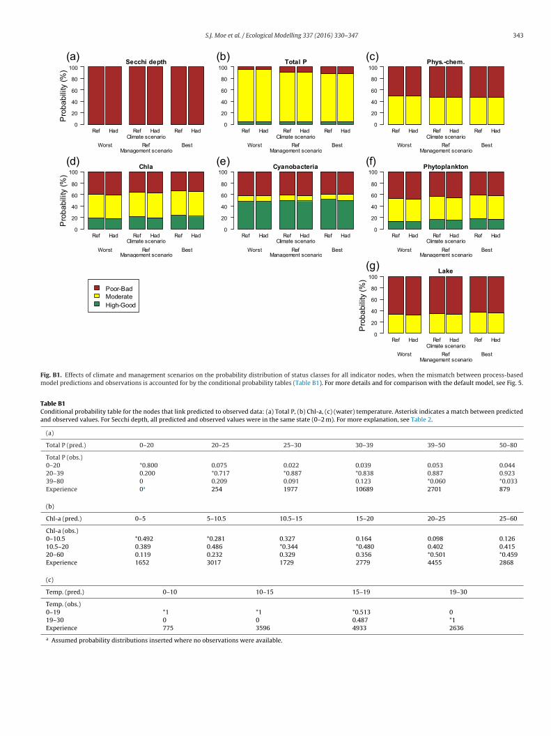
alues in the CPTs (Table B1) had clear consequences for the BNodel predictions (BN version 2, Fig. B1). For TP (Fig. B1b), the BN

o longer predicted a positive effect of better management on therobability of moderate status, but instead a weak increase in therobability of poor-bad status. For the combined physical-chemical

ndicator (Fig. B1c) there was no obvious response to the manage-ent scenarios. The Chl-a variable (Fig. B1d) and thus the combined

hytoplankton indicator (Fig. B1f) displayed similar responses tohe management scenarios as in the default BN version (Fig. 5dnd f), but the effects of the scenarios were much weaker. This isonsistent with the high accuracy and low precision of predictedhl-a from the process-based model. The total lake assessment wasost dominated by the phytoplankton node (as determined by

he classification rules), but the physical-chemical indicator con-ributed with additional uncertainty. In the BN version 2, the overallake assessment for the reference scenario (Fig. B1g) was close tohe default version (Fig. 5g), but there was almost no effect of the

anagement or climate scenarios. This is a common problem forN models that incorporate several sources of uncertainty: nodes

urther down the causal chain have greater predictive uncertaintyBorsuk et al., 2004; Marcot et al., 2006).

Our decision not to include the mismatch between MyLakeredictions and observations in the default BN version can be jus-ified by the fact that this uncertainty should already have beenccounted for in the calibration of MyLake. The resulting 60 param-ter sets were instead included as a source of uncertainty in the BN.ncorporating the prediction − observation mismatch as an addi-ional source of uncertainty would not only make the BN modelon-responsive to the scenarios, but also introduce a systematicrror for TP.

.2.2. The CPT for cyanobacteriaA minority of the EUREGI observations were from lakes with

igh degree of eutrophication; only 45 out of 559 observations weren the highest Chl-a interval (vs. 34 out of 90 observations from Lakeansjø). Likewise, the number of cyanobacteria observations in theighest interval was relatively low: 22 out of 559 (vs. 13 out of 90

rom Lake Vansjø). Nevertheless, the EUREGI dataset gave similarrobability distributions in the CPT for cyanobacteria (Table B2) tohose from Lake Vansjø (Table 2b-c). Consequently, model version

with CPT from the EUREGI dataset predicted effects of climatend management scenarios on ecological status of cyanobacte-ia (Fig. B2e) that were very similar to the default model versionFig. 5e). The fact that an independent, large-scale dataset gaveimilar CPTs and consequently very similar model predictions ashe original data from Lake Vansjø strengthened our confidence inhe cyanobacteria component of the model.

.2.3. Effects of water temperatureSince the future climate scenario had a limited effect of the

emperature node (probability of “a warm year” increased from4% to 44%), we investigated more closely how the phytoplanktonodes responded to changes in water temperature in the model.ne way to inspect the temperature effects in the BN was to select

he warmest months, July-August (“summer”). The full model isased on all data from May to October, because this is a criterion

n the national assessment system for ecological status. However,ince there is large seasonal variation in many of the variables,electing only summer months would reduce the temporal vari-tion, and might therefore improve the precision of the model (i.e.,

ling 337 (2016) 330–347

result in narrower probability distributions of the indicators). Wetherefore compared the default model outcome (Fig. 5) with thecorresponding results from summer months (Fig. B3). (To simplifythe comparison we have displayed the result in terms of statusclasses, although it is not strictly correct to base the status assess-ment of summer values only). Lower probability of Moderate orbetter status can be seen for all indicators, except cyanobacteria;this is likely because Cyanobacteria status is based on the seasonalmaximum, which is less sensitive to the selection of months. Thisresult shows that the model behaves as expected regarding sea-sonal variation in temperature and in indicator variables.

Further inspection of the water temperature effects was per-formed by setting evidence for “a warm year” (100% probability oftemperature ≥ 19 ◦C) vs. “a cold year” (<19 ◦C) (Fig. B4). The tem-perature effect was stronger for Chl-a than for cyanobacteria: froma cold to a warm year, the probability of moderate or better Chl-a status dropped from 58% to 24% (worst management) and from70% to 48% (best management). The corresponding probabilitiesfor cyanobacteria were a drop from 64% to 47% (worst manage-ment) and from 71% to 60% (best management), but this responseincluded both the direct effect of the temperature node and theindirect temperature effect through the Chl-a node. Furthermore,we fixed the Chl-a node at PB, M or HG status under cold and warmyear, respectively (Fig. B5a). The additional temperature effect oncyanobacteria was most evident when Chl-a was in moderate sta-tus (Fig. B5b). This result is in line with the conclusion by Rigosi et al.(2015), that the cyanobacteria concentrations of mesotrophic lakeswere particularly sensitive to warming. This temperature effect oncyanobacteria had a small, but noticeable effect on the total phyto-plankton status (Fig. B5c). Although this effect was small, it showsthat the BN generated reasonable results.

4.3. Assessment of the BN approach for modelling of ecologicalstatus

Overall, the BN model satisfied our objective: to integrate infor-mation from scenarios, process-based models, monitoring data –especially cyanobacteria, and the lake classification system. TheBN approach gives a possibility to account for mismatch betweenprocess-model predictions and observations for certain variables,by incorporating this uncertainty in their CPTs (cf. Table B1) andevaluating its consequences. Since the selected model (version 1)does not account for the mismatch between MyLake predictionand observations, the results predicted by the BN should not beinterpreted in terms of absolute probability values. Nevertheless,the qualitative effects of the scenarios on the different indicatorspredicted by the BN should be valid.

The components involving cyanobacteria gave reasonableresults, and had importance to the overall assessment. Our con-fidence in these components was strengthened by the comparisonwith an independent dataset (Fig. B2); at the coarse scale of the eco-logical status (rather than exact concentrations), the results werevery similar. This implies that our approach can be used for otherlakes that are at risk of algal blooms. For lakes with more lim-ited data on cyanobacteria than Lake Vansjø, we show that fillingthe data gaps using cyanobacteria observations from other lakesin combination with expert knowledge on lake type, local condi-tions etc. is a viable option. Rigosi et al. (2015) demonstrated thispossibility: using physicochemical, biological, and meteorologicalobservations collated from 20 lakes located at different latitudesand characterized by a range of sizes and trophic states, they con-
structed a BN to analyse the sensitivity of cyanobacterial bloomdevelopment to different environmental factors and to determinethe probability that cyanobacterial blooms would occur. The abil-ity to utilize other available datasets for answering management

Model

qs

ima“swlotucht(ct

ttwllr2mtbas2cectgto

tmppdFdpfMatccv1

AuMsw2BL


uestions is a strength of the BN approach, given the financial con-traints of most agencies (Wilson et al., 2008).

A complete ecological status assessment should in principlenclude three more biological quality elements (BQEs), namely

acrophytes, benthic invertebrates and fish (EC, 2000). Such anssessment is likely to have resulted in even worse status, due to theone-out, all-out” combination rule of the WFD (EC, 2005). This ruletates that the ecological status should be determined by the BQEith lowest status, meaning that including more BQEs inevitably

eads to a stricter or equally strict assessment. The more pessimisticutcome of the one-out, all-out rule compared to other combina-ion rules was also demonstrated by Lehikoinen et al. (2014), whosed a BN for analysing the probability of reaching good ecologi-al status of coastal waters in the Gulf of Finland. When there isigh uncertainty associated with the data, assessments based onhis combination rule tend to underestimate the ecological statusMoe et al., 2015). A probabilistic result such as the outcome of a BNan be helpful, giving a more nuanced and more informative resulthan only a single status class (Gottardo et al., 2011).

Compared to existing process-based models for ecological sta-us of rivers and lakes, the BN approach provides an opportunityo include biological elements, as demonstrated by our study. Evenhen data are sparse, theory or expert knowledge on selected bio-

ogical indicators can be used as a first step to construct causalinks (CPTs) between abiotic and biotic responses. Since the WFDequires that assessments are based primarily on biology (EC,000), this is clearly an added value for use of models in wateranagement in Europe. Moreover, the WFD requires that poten-

ial impacts of climate change are considered in the next set of riverasin management plans (EC, 2009). Although much knowledge isvailable on effects on climate change on ecosystems, includingpecific effects on biological quality elements in lakes (Moe et al.,014), incorporating such information in predictive models is ahallenge. The BN methodology can facilitate the use of such knowl-dge, manifested as expert judgement of probabilities under givenlimatic scenarios. Furthermore, a BN model may be relatively easyo understand for end users who do not have any modelling back-round {Borsuk et al., 2012 #138}. Therefore, BNs are promisingools for supporting informed decision making and thus the workf water managers.

There are of course also several limitations associated withhe BN methodology in the context of environmental manage-

ent. The fact that the non-dynamic network cannot contain loopsuts constraints on the ecological processes that can be modelled;hosphorus and phytoplankton dynamics in lakes are typicallyominated by feedback processes (Saloranta and Andersen, 2007).or example, high phytoplankton biomass can reduce the Secchiepth; on the other hand, lower Secchi depth can limit furtherhytoplankton growth due to light limitation. In our study, sucheedback loops were handled by dynamic models (INCA-P and

yLake), while the BN summarised the outcome of the catchmentnd lake process. Moreover, the accumulation of uncertainty withhe length of the network implies that it can be difficult to drawonclusions from the final output nodes (Borsuk et al., 2004). Otherhallenges associated with the use of BNs have been discussed pre-iously (Landuyt et al., 2013; Uusitalo, 2007; Varis and Kuikka,999).

The current BN model can be further developed in several ways.n important improvement would be to reduce the predictivencertainty of the catchment-lake model chain (i.e. INCA-P andyLake). A more quantitative sensitivity analysis of the model,

uch as calculation of entropy reduction, can help identify nodes to
hich the final output is particularly sensitive (Chen and Pollino,
012). A more complete representation of climate change in theN would include effects of changed precipitation patterns (cf.ehikoinen et al., 2014), and potentially other meteorological

ling 337 (2016) 330–347 341

or hydrological variables. Inclusion of Total N in the BN wouldmake the assessment of physico-chemical status more complete.The total N concentration also seems to play a role in favour-ing certain N-fixating cyanobacteria taxa (order Nostocales, e.g.Anabaena), especially in late summer/autumn after N has beendepleted. Effects of nutrients and other environmental variableson Anabaena biomass in a reservoir were recently analysed byanother BN model (Williams and Cole, 2013): reduced levels ofN and/or P had negligible impact on the phytoplankton in theirstudy, while high water temperature and stratification increasedthe risk of Anabaena blooms. Anyway, to model effects of climateor management scenarios on Total N in our BN would require thatthis variable is first incorporated in the process-based lake model.Finally, a dynamic version of the BN could be considered (Molinaet al., 2013; Nicholson and Flores, 2011), which might better handlefeedback processes.

In this study we used an external, larger dataset for evaluationby constructing an alternative CPT for cyanobacteria and compar-ing the results with the default model version. External datasetscan also be used in a more integrated way for estimation of CPTs.However, differences in lake type factors such as water colourand alkalinity may be even more important than the TP concen-tration (Carvalho et al., 2011). A hierarchical Bayesian regressionmodel would be a suitable method for estimating relationshipsfor a target lake while “borrowing information” on this type ofrelationship from a larger set of lakes, and simultaneously account-ing for differences in lake type (Kotamäki et al., 2015). Inclusionof more biological quality elements would also be desirable; pri-marily macrophytes, for which some data exist (Haande et al.,2011). Future monitoring in Lake Vansjø might provide some morebiological data also for macrophytes and fish. However, new bio-logical elements for which few observations are available will beassociated with high uncertainty. The model structure in its cur-rent version is rather simple and general, and should be feasibleto adapt for other lakes or other aquatic ecosystems. The modelcan be considered over-fitted to Lake Vansjø, since the estimationof probability distributions is based solely on data from this casestudy. Application of this model to other ecosystems should involvecalibration and validation of the model with relevant data.

4.4. Conclusions

In summary, the Bayesian network approach was able to modeleffects of climate change and management on ecological statusof a lake, by combining scenarios, process-based model output,monitoring data and the national lake assessment system. The BNmodel showed that the benefits of better land-use managementwere partly counteracted by future warming under these scenar-ios. Most importantly, the BN demonstrated the importance ofincluding more biological elements, namely cyanobacteria, in themodelling of lake status. Thus, the BN modelling approach can bea useful supplement to more traditional process-based models forlakes, which only rarely include cyanobacteria or other biologicalgroups.

Acknowledgements

We are grateful to David Barton, Andrew Wade and RichardSkeffington for discussions on the model structure, Koji Tominagafor providing output from the MyLake model, Anne Lyche Sol-heim for information on the national classification system and
Peter Friis Hansen for technical help with the Hugin software.The authors have received funding from the projects REFRESH(Adaptive Strategies to Mitigate the Impacts of Climate Change onEuropean Freshwater Ecosystems; EU FP7, contract no. 244121),

3 Model

Mmfnpf

An

Is

sit1

Appendix B

TC(


ARS (Managing Aquatic ecosystems and water Resources underultiple Stress; EU FP7, contract no. 603378), Climate effects

rom mountains to fjords (Research Council of Norway projecto. 208279) and Lakes in Transition (Research Council of Norwayroject no. 244558/E50). We also thank two anonymous reviewersor their many helpful comments.

ppendix A. Implementation of combination rules of theational classification system

mplementation of combination rules of the national classificationystem

For the combined Physico-Chemical status, the classification
ystem requires averaging of the two variables Secchi and TP, whichs not straight-forward in a probabilistic model. When both indica-ors had the same status, the combined status was the same with00% probability. The averaging was implemented by assigning
able A1onditional probability tables for the national classification system for ecological status

d) Status Cyano, (e) Status Phys-Chem, (f) Status Phytoplankton. (For the node Status of

(a)

Secchi 0–2 2–2.6

Status SecchiHG 0 0

M 0 1

PB 1 0

(b)

Total P 0–20 20–39

Status Total PHG 1 0

M 0 1

PB 0 0

(c)

Chl-a 0–10.5 10.5–20

Status Chl-aHG 1 0

M 0 1

PB 0 0

(d)

CyanoMax 0–1000 1000–2000

Status CyanoHG 1 0

M 0 1

PB 0 0

(e)

Status Total P HG M

Status Secchi HG M PB HGStatus Phys-chem.HG 1 0.5 0 0.5M 0 0.5 1 0.5PB 0 0 0 0

(f)

Status Chl-a HG M

Status Cyano HG M PB HGStatus PhytoplanktonHG 1 0.5 0 0

M 0 0.5 1 1

PB 0 0 0 0

ling 337 (2016) 330–347

50% probability of both High-Good and Moderate status when oneindicator was in High-Good status and the other was in Moderatestatus, and likewise for Moderate and Poor-Bad status (Table A1e).When one indicator was High-Good and the other Poor-Bad, thecombined status was Moderate with 100% probability. For the com-bined Phytoplankton status, a similar solution was used, with someexceptions: when the status of Cyano was better than or equal tothe status of Chl-a, the combined status was set equal to the statusof Chl-a (Table A1f). The overall lake status (Table 2d) was set equalto the phytoplankton status when the physico-chemical status wasequal or better, and to one lower state when the physico-chemicalstatus was worse.

Figs. B1–B5 .Tables B1 and B2.

of lakes (see Fig. 2, Module 4). (a) Status Secchi, (b) Status Total P, (c) Status Chl-a,Lake, see Table 1e). HG = High-Good, M = Moderate, PB = Poor-Bad.

2.6–5

100

39–80

001

20–60

001

2000–6000

001

PB

M PB HG M PB

0 0 0 0 0 1 0.5 1 0.5 0

0 0.5 0 0.5 1

PB

M PB HG M PB

0 0 0 0 01 0.5 0 0 00 0.5 1 1 1


0

20

40

60

80

100



Secc hi depthP

roba

bilit

y (%

)(a)

0

20

40

60

80

100



Total P(b)

0

20

40

60

80

100



Phys.-chem.(c)

0

20

40

60

80

100



Chla

Pro

babi

lity

(%)

(d)

0

20

40

60

80

100



Cyanobacteria(e)

0

20

40

60

80

100



Phytop lankton(f)


0

20

40

60

80

100



Lake

Pro

babi

lity

(%)

(g)

Fig. B1. Effects of climate and management scenarios on the probability distribution of status classes for all indicator nodes, when the mismatch between process-basedmodel predictions and observations is accounted for by the conditional probability tables (Table B1). For more details and for comparison with the default model, see Fig. 5.

Table B1Conditional probability table for the nodes that link predicted to observed data: (a) Total P, (b) Chl-a, (c) (water) temperature. Asterisk indicates a match between predictedand observed values. For Secchi depth, all predicted and observed values were in the same state (0–2 m). For more explanation, see Table 2.

(a)

Total P (pred.) 0–20 20–25 25–30 30–39 39–50 50–80

Total P (obs.)0–20 *0.800 0.075 0.022 0.039 0.053 0.04420–39 0.200 *0.717 *0.887 *0.838 0.887 0.92339–80 0 0.209 0.091 0.123 *0.060 *0.033Experience 0a 254 1977 10689 2701 879

(b)

Chl-a (pred.) 0–5 5–10.5 10.5–15 15–20 20–25 25–60

Chl-a (obs.)0–10.5 *0.492 *0.281 0.327 0.164 0.098 0.12610.5–20 0.389 0.486 *0.344 *0.480 0.402 0.41520–60 0.119 0.232 0.329 0.356 *0.501 *0.459Experience 1652 3017 1729 2779 4455 2868

(c)

Temp. (pred.) 0–10 10–15 15–19 19–30

Temp. (obs.)0–19 *1 *1 *0.513 0
19–30 0 0
Experience 775 3596

a Assumed probability distributions inserted where no observations were available.

0.487 *1
4933 2636


0

20

40

60

80

100



Secc hi depthP

roba

bilit

y (%

)(a)

0

20

40

60

80

100



Total P(b)

0

20

40

60

80

100



Phys.-chem.(c)

0

20

40

60

80

100



Chla

Pro

babi

lity

(%)

(d)

0

20

40

60

80

100



Cyanobacteria(e)

0

20

40

60

80

100



Phytop lankton(f)


0

20

40

60

80

100



Lake

Pro

babi

lity

(%)

(g)

Fig. B2. Effects of climate and management scenarios on the probability distribution of status classes for all indicator nodes, when the conditional probability table forCyanobacteria is based on the alternative larger dataset EUREGI (see section 2.2.3). For more details and for comparison with the default model, see Fig. 5.

Table B2Conditional probability table for the two cyanobacteria nodes based on the alternative, larger dataset (EUREGI, see section 2.2.3): (a) Cyano, (b) CyanoMax (corresponding toTable 2c and d, respectively). For more information, see Table 2.

(a)

Chl-a (obs.) 0–10.5 10.5–20 20–60

Temp. (obs.) 0–19 19–30 0–19 19–30 0–19 19–30Cyano0–1000 0.993 1 0.949 1 0.444 0.1111000–2000 0.007 0 0.051 0 0.111 0.2222000–6000 0 0 0 0 0.444 0.667Experience 454 19 39 2 36 9

(b)

Cyano 0–1000 1000–2000 2000–6000

Season May–Jun Jul–Aug Sep–Oct May–Jun Jul–Aug Sep–Oct May–Jun Jul–Aug Sep–OctCyanoMax0–1000 0.882 0.964 0.870 0 0 0 0 0 0
1000–2000 0.076 0.034 0.087 0.5
2000–6000 0.042 0.003 0.043 0.5

Experience 119 384 23 2

0.889 0 0 0 0
0.111 0 1 1 19 0 5 16 1


0

20

40

60

80

100



Secc hi depthP

roba

bilit

y (%

)(a)

0

20

40

60

80

100



Total P(b)

0

20

40

60

80

100



Phys.-chem.(c)

0

20

40

60

80

100



Chla

Pro

babi

lity

(%)

(d)

0

20

40

60

80

100



Cyanobacteria(e)

0

20

40

60

80

100



Phytop lankton(f)


0

20

40

60

80

100



Lake

Pro

babi

lity

(%)

(g)

Fig. B3. Effects of climate and management scenarios on the probability distribution of status classes for all indicator nodes, when the model is run only for the warmestmonths (July–August). For more details and for comparison with the default model, see Fig. 5.

0

20

40

60

80

100

Cold Warm Cold WarmCold vs. w arm yea r

Worst BestManage ment scena rio

Chla

Pro

babi

lity

(%)

(a)

0

20

40

60

80

100



Cyanob acteria(b)

0

20

40

60

80

100



Phytoplankton(c)


Fo

ig. B4. Effects of high vs. low water temperature (above vs. below 19 ◦C, respectively) unf status classes for Chl-a (a), Cyanobacteria (b) and Phytoplankton (c). For more details a

der different management scenarios (worst vs. best) on the probability distributionnd for comparison with the default model, see Fig. 5.


0

20

40

60

80

100

C W C W C WCold vs. w arm yea r

PB M HGChla status

Chla(a)

Pro

babi

lity

(%)

0

20

40

60

80

100


PB M HGChla status

Cyanobacteria(b)

0

20

40

60

80

100


PB M HGChla status

Phytoplankton(c)


F ely) up lankto

A

adgtSt0

R

A

A

B

B

B

B

B

B

C

C

C

C

C

ig. B5. Effects of high vs. low water temperature (above vs. below 19 ◦C, respectivrobability distribution of status classes for Chl-a (a), Cyanobacteria (b) and Phytop

ppendix C. Supplementary data

The file Supplementary Data.pdf contains tables with prior prob-bility distributions for all parent nodes and conditional probabilityistributions for all child nodes. The probability distributions areiven as counts rather than proportions. The file is generated fromhe BN model by the software Hugin.upplementary data associated with this article can be found, inhe online version, at http://dx.doi.org/10.1016/j.ecolmodel.2016.7.004.

eferences

guilera, P.A., Fernández, A., Fernández, R., Rumí, R., Salmerón, A., 2011. Bayesiannetworks in environmental modelling. Environ. Model. Softw. 26, 1376–1388.

rheimer, B., Andréasson, J., Fogelberg, S., Johnsson, H., Pers, C., Persson, K., 2005.Climate change impact on water quality: model results from southern Sweden.Ambio 34, 559–566.

arton, D.N., Kuikka, S., Varis, O., Uusitalo, L., Henriksen, H.J., Borsuk, M., de la Hera,A., Farmani, R., Johnson, S., Linnell, J.D.C., 2012. Bayesian networks inenvironmental and resource management. Integr. Environ. Assess. Manage. 8,418–429.

arton, D.N., Saloranta, T., Bakken, T.H., Solheim, A.L., Moe, J., Selvik, J.R., Vagstad,N., 2005. Using bayesian network models to incorporate uncertainty in theeconomic analysis of pollution abatement measures under the WaterFramework Cirective. Water Supply 5, 99–104.

arton, D.N., Saloranta, T., Moe, S.J., Eggestad, H.O., Kuikka, S., 2008. Bayesian beliefnetworks as a meta-modelling tool in integrated river basinmanagement—pros and cons in evaluating nutrient abatement decisions underuncertainty in a Norwegian river basin. Ecol. Econ. 66, 91–104.

arton, D.N., Andersen, T., Bergland, O., Engebretsen, A., Moe, J., Orderud, G.,Tominaga, K., Romstad, E., Vogt, R., 2014. Eutropia—integrated valuation oflake eutrophication abatement decisions using a Bayesian belief network. In:Applied System Science Applied System Science.

orsuk, M.E., Stow, C.A., Reckhow, K.H., 2004. A Bayesian network ofeutrophication models for synthesis prediction, and uncertainty analysis. Ecol.Model. 173, 219–239.

orsuk, M.E., Schweizer, S., Reichert, P., 2012. A Bayesian network model forintegrative river rehabilitation planning and management. Integr. Environ.Assess. Manage. 8, 462–472.

arvalho, L., McDonald, C., de Hoyos, C., Mischke, U., Phillips, G., Borics, G., Poikane,S., Skjelbred, B., Solheim, A.L., Van Wichelen, J., Cardoso, A.C., 2013. Sustainingrecreational quality of European lakes: minimizing the health risks from algalblooms through phosphorus control. J. Appl. Ecol. 50, 315–323.

arvalho, L., Miller, C.A., Scott, E.M., Codd, G.A., Davies, P.S., Tyler, A.N., 2011.Cyanobacterial blooms: statistical models describing risk factors fornational-scale lake assessment and lake management. Sci. Total Environ. 409,5353–5358.

astelletti, A., Soncini-Sessa, R., 2007. Bayesian Networks and participatorymodelling in water resource management. Environ. Model. Softw. 22,1075–1088.

hen, S.H., Pollino, C.A., 2012. Good practice in Bayesian network modelling.
Environ. Model. Softw. 37, 134–145.
outure, R.M., Tominaga, K., Starrfelt, J., Moe, S.J., Kaste, O., Wright, R.F., 2014.Modelling phosphorus loading and algal blooms in a Nordic agriculturalcatchment-lake system under changing land-use and climate. Environ. Sci.Process. Impacts 16, 1588–1599.

nder different scenarios of chl-a status (Poor-Bad, Moderate or Good-High) on then (c). For more details and for comparison with the default model, see Fig. 5.

Davis, T.W., Berry, D.L., Boyer, G.L., Gobler, C.J., 2009. The effects of temperatureand nutrients on the growth and dynamics of toxic and non-toxic strains ofMicrocystis during cyanobacteria blooms. Harmful Algae 8, 715–725.

EC (European Commission), 2000. Directive 2000/60/EC of the EuropeanParliament and of the Council of 23 October 2000 Establishing a Framework forCommunity Action in the Field of Water Policy. EC, Luxembourg.

EC (European Commission), 2005. Overall Approach to the Classification ofEcological Status and Ecological Potential. EC, Luxembourg.

EC (European Commission), 2009. River Basin Management in a Changing Climate.Common Implementation Strategy for the Water Framework DirectiveGuidance Document Number 24. EC (134 pp).

Elliott, J.A., 2010. The seasonal sensitivity of cyanobacteria and otherphytoplankton to changes in flushing rate and water temperature. GlobalChange Biol. 16, 864–876.

Elliott, J.A., 2012. Is the future blue-green: a review of the current modelpredictions of how climate change could affect pelagic freshwatercyanobacteria. Water Res. 46, 1364–1371.

Elliott, J.A., May, L., 2008. The sensitivity of phytoplankton in Loch Leven (U.K.) tochanges in nutrient load and water temperature. Freshw. Biol. 53, 32–41.

French, R.H., Cooper, J.J., Vigg, S., 1982. Secchi disc relationships. JAWRA J. Am.Water Resour. Assoc. 18, 121–123.

Futter, M.N., Erlandsson, M.A., Butterfield, D., Whitehead, P.G., Oni, S.K., Wade, A.J.,2013. PERSiST: the precipitation, evapotranspiration and runoff simulator forsolute transport. Hydrol. Earth Syst. Sci. Discuss. 10, 8635–8681.

Gal, G., Hipsey, M., Rinke, K., Robson, B., 2014. Novel approaches to addresschallenges in modelling aquatic ecosystems. Environ. Model. Softw. 61,246–248.

Gottardo, S., Semenzin, E., Giove, S., Zabeo, A., Critto, A., de Zwart, D., Ginebreda, A.,Marcomini, A., 2011. Integrated risk assessment for WFD ecological statusclassification applied to Llobregat river basin (Spain). Part I—fuzzy approach toaggregate biological indicators. Sci. Total Environ. 409, 4701–4712.

Haande, S., Solheim, A., Moe, J., Brænden, R., Lyche Solheim, A., Moe, J., Brænden, R.,2011. Klassifisering av økologisk tilstand i elver og innsjøer i VannområdeMorsa iht. Vanndirektivet. (Classification of ecologial status in rivers and lakesin river basin Morsa according to the Water Framework Directive). NIVA reportno. 6166. NIVA report no. 6166.

Hering, D., Borja, A., Carvalho, L., Feld, C.K., 2013. Assessment and recovery ofEuropean water bodies: key messages from the WISER project. Hydrobiologia704, 1–9.

Hothorn, T., Hornik, K., Zeileis, A., 2006. Unbiased recursive partitioning: aconditional inference framework. J. Comput. Graph. Stat. 15, 651–674.

Howard, A., Easthope, M.P., 2002. Application of a model to predict cyanobacterialgrowth patterns in response to climatic change at Farmoor Reservoir,Oxfordshire, UK. Sci. Total Environ. 282–283, 459–469.

Huber, V., Wagner, C., Gerten, D., Adrian, R., 2012. To bloom or not to bloom:contrasting responses of cyanobacteria to recent heat waves explained bycritical thresholds of abiotic drivers. Oecologia 169, 245–256.

Jackson-Blake, L.A., Dunn, S.M., Helliwell, R.C., Skeffington, R.A., Stutter, M.I., Wade,A.J., 2015. How well can we model stream phosphorus concentrations inagricultural catchments? Environ. Model. Softw. 64, 31–46.

Jeppesen, E., Kronvang, B., Meerhoff, M., Søndergaard, M., Hansen, K.M., Andersen,H.E., Lauridsen, T.L., Liboriussen, L., Beklioglu, M., Özen, A., Olesen, J.E., 2009.Climate change effects on runoff, catchment phosphorus loading and lakeecological state, and potential adaptations. J. Environ. Qual. 38, 1930–1941.

Jeppesen, E., Meerhoff, M., Holmgren, K., Gonzalez-Bergonzoni, I., Teixeira-deMello, F., Declerck, S.A.J., De Meester, L., Sondergaard, M., Lauridsen, T.L.,
Bjerring, R., Conde-Porcuna, J.M., Mazzeo, N., Iglesias, C., Reizenstein, M.,Malmquist, H.J., Liu, Z.W., Balayla, D., Lazzaro, X., 2010. Impacts of climatewarming on lake fish community structure and potential effects on ecosystemfunction. Hydrobiologia 646, 73–90.
http://dx.doi.org/10.1016/j.ecolmodel.2016.07.004











http://refhub.elsevier.com/S0304-3800(16)30246-0/sbref0005





































































































































































































































































































































































































































































































































































































































































Model

J

K

KK

L

L

L

L

M

M

M

M

M

M

M

M

M

M

M

M

N

N

Williams, B.J., Cole, B., 2013. Mining monitored data for decision-making with aBayesian network model. Ecol. Model. 249, 26–36.


eppesen, E., Mehner, T., Winfield, I.J., Kangur, K., Sarvala, J., Gerdeaux, D., Rask, M.,Malmquist, H.J., Holmgren, K., Volta, P., Romo, S., Eckmann, R., Sandström, A.,Blanco, S., Kangur, A., Ragnarsson Stabo, H., Tarvainen, M., Ventelä, A.-M.,Søndergaard, M., Lauridsen, T.L., Meerhoff, M., 2012. Impacts of climatewarming on the long-term dynamics of key fish species in 24 European lakes.Hydrobiologia 694, 1–39.

eshtkar, A.R., Salajegheh, A., Sadoddin, A., Allan, M.G., 2013. Application ofBayesian networks for sustainability assessment in catchment modeling andmanagement (Case study: the Hablehrood river catchment). Ecol. Model. 268,48–54.

oski, T., Noble, J., 2009. Bayesian Networks: An Introduction. Wiley (366 pp).otamäki, N., Pätynen, A., Taskinen, A., Huttula, T., Malve, O., 2015. Statistical

dimensioning of nutrient loading reduction: LLR assessment tool for lakemanagers. Environ. Manage. 56, 480–491.

anduyt, D., Broekx, S., D’Hondt, R., Engelen, G., Aertsens, J., Goethals, P.L.M., 2013.A review of Bayesian belief networks in ecosystem service modelling. Environ.Model. Softw. 46, 1–11.

ecklin, T., Ryömä, R., Kuikka, S., 2011. A Bayesian network for analyzing biologicalacute and long-term impacts of an oil spill in the Gulf of Finland. Mar. Pollut.Bull. 62, 2822–2835.

ehikoinen, A., Helle, I., Klemola, E., Mäntyniemi, S., Kuikka, S., Pitkänen, H., 2014.Evaluating the impact of nutrient abatement measures on the ecological statusof coastal waters: a Bayesian network for decision analysis. Int. J. MulticriteriaDeci. Mak. 4, 114–134.

ehikoinen, A., Luoma, E., Mäntyniemi, S., Kuikka, S., 2013. Optimizing the recoveryefficiency of Finnish oil combating vessels in the Gulf of Finland using Bayesiannetworks. Environ. Sci. Technol. 47, 1792–1799.

arcot, B.G., 2012. Metrics for evaluating performance and uncertainty of Bayesiannetwork models. Ecol. Model. 230, 50–62.

arcot, B.G., Steventon, J.D., Sutherland, G.D., McCann, R.K., 2006. Guidelines fordeveloping and updating Bayesian belief networks applied to ecologicalmodeling and conservation. Can. J. For. Res. 36, 3063–3074.

arkensten, H., Pierson, D.C., 2007. Weather driven influences on phytoplanktonsuccession in a shallow lake during contrasting years: application of PROTBAS.Ecol. Model. 207, 128–136.

artín de Santa Olalla, F., Dominguez, A., Ortega, F., Artigao, A., Fabeiro, C., 2007.Bayesian networks in planning a large aquifer in Eastern Mancha, Spain.Environ. Model. Softw. 22, 1089–1100.

erel, S., Walker, D., Chicana, R., Snyder, S., Baures, E., Thomas, O., 2013. State ofknowledge and concerns on cyanobacterial blooms and cyanotoxins. Environ.Int. 59, 303–327.

oe, S.J., 2010. Bayesian models in assessment and management. In: Kapustka, L.,Landis, W.G., Johnson, A. (Eds.), Environmental Risk Assessment andManagement from a Landscape Perspective. Wiley’s.

oe, S.J., Bennion, H., Cid, N., Solheim, A.L., Nõges, P., Adrian, R., Cardoso, A.C.,Brucet, S., Tuvikene, L., Persson, J., 2014. Implications of climate change forecological reference conditions, thresholds and classifiation systems forEuropean lakes. REFESH Deliv. 3 (15–16), 108 http://www.refresh.ucl.ac.uk/Deliverable+3.15 abstract.

oe, S.J., Lyche Solheim, A., Soszka, H., Gołub, M., Hutorowicz, A., Kolada, A.,Picinska-Fałtynowicz, J., Białokoz, W., 2015. Integrated assessment ofecological status and misclassification of lakes: the role of uncertainty andindex combination rules. Ecol. Indic. 48, 605–615.

olina, J.-L., Pulido-Velázquez, D., García-Aróstegui, J.L., Pulido-Velázquez, M.,2013. Dynamic Bayesian networks as a decision support tool for assessingclimate change impacts on highly stressed groundwater systems. J. Hydrol.479, 113–129.

olina, J.L., Bromley, J., García-Aróstegui, J.L., Sullivan, C., Benavente, J., 2010.Integrated water resources management of overexploited hydrogeologicalsystems using Object-Oriented Bayesian Networks. Environ. Model. Softw. 25,383–397.

ooij, W., Trolle, D., Jeppesen, E., Arhonditsis, G., Belolipetsky, P., Chitamwebwa,D.R., Degermendzhy, A., DeAngelis, D., De Senerpont Domis, L., Downing, A.,Elliott, J.A., Fragoso Jr., C., Gaedke, U., Genova, S., Gulati, R., Håkanson, L.,Hamilton, D., Hipsey, M., ‘t Hoen, J., Hülsmann, S., Los, F.H., Makler-Pick, V.,Petzoldt, T., Prokopkin, I., Rinke, K., Schep, S., Tominaga, K., Van Dam, A., VanNes, E., Wells, S., Janse, J., 2010. Challenges and opportunities for integratinglake ecosystem modelling approaches. Aquat. Ecol. 44, 633–667.

ooij, W.M., Janse, J.H., Senerpont Domis, L.N., Hülsmann, S., Ibelings, B.W., 2007.Predicting the effect of climate change on temperate shallow lakes with theecosystem model PCLake. Hydrobiologia 584, 443–454.

icholson, A.E., Flores, M.J., 2011. Combining state and transition models with
dynamic Bayesian networks. Ecol. Model. 222, 555–566.
õges, P., Mischke, U., Laugaste, R., Solimini, A.G., 2010. Analysis of changes over44 years in the phytoplankton of Lake Võrtsjärv (Estonia): the effect ofnutrients, climate and the investigator on phytoplankton-based water qualityindices. Hydrobiologia 646, 33–48.

ling 337 (2016) 330–347 347

Oredalen, T.J., Faafeng, B., 2002. Landsomfattende undersøkelse av trofitilstanden inorske innsjøer. Datarapport 2001, 4570.

Paerl, H.W., Huisman, J., 2008. Blooms like it hot. Science 320, 57–58.Phillips, G., Pietiläinen, O.P., Carvalho, L., Solimini, A., Lyche Solheim, A., Cardoso,

A.C., 2008. Chlorophyll–nutrient relationships of different lake types using alarge European dataset. Aquat. Ecol. 42, 213–226.

Poikane, S., Birk, S., Böhmer, J., Carvalho, L., de Hoyos, C., Gassner, H., Hellsten, S.,Kelly, M., Lyche Solheim, A., Olin, M., Pall, K., Phillips, G., Portielje, R.,Ritterbusch, D., Sandin, L., Schartau, A.-K., Solimini, A.G., van den Berg, M.,Wolfram, G., van de Bund, W., 2015. A hitchhiker’s guide to European lakeecological assessment and intercalibration. Ecol. Indic. 52, 533–544.

Pollino, C.A., Henderson, C., 2010. Bayesian Networks: A Guide for TheirApplication in Natural Resource Management and Policy. Landscape Logic,Australian Government Department of the Environment, Water, Heritage andthe Arts, Canberra, Australia.

Ptacnik, R., Lepistö, L., Willén, E., Brettum, P., Andersen, T., Rekolainen, S., LycheSolheim, A., Carvalho, L., 2008. Quantitative responses of lake phytoplankton toeutrophication in Northern Europe. Aquat. Ecol. 42, 227–236.

Ptacnik, R., Solimini, A., Brettum, P., 2009. Performance of a new phytoplanktoncomposition metric along a eutrophication gradient in Nordic lakes.Hydrobiologia 633, 75–82.

R Core Team, 2015. R: A Language and Environment for Statistical Computing. RFoundation for Statistical Computing, Vienna, Austria http://www.R-project.org/.

Recknagel, F., Ostrovsky, I., Cao, H., 2014. Model ensemble for the simulation ofplankton community dynamics of Lake Kinneret (Israel) induced from in situpredictor variables by evolutionary computation. Environ. Model. Softw. 61,380–392.

Rigosi, A., Hanson, P., Hamilton, D.P., Hipsey, M., Rusak, J.A., Bois, J., Sparber, K.,Chorus, I., Watkinson, A.J., Qin, B., Kim, B., Brookes, J.D., 2015. Determining theprobability of cyanobacterial blooms: the application of Bayesian networks inmultiple lake systems. Ecol. Appl. 25, 186–199.

Saloranta, T.M., Andersen, T., 2007. MyLake—a multi-year lake simulation modelcode suitable for uncertainty and sensitivity analysis simulations. Ecol. Model.207, 45–60.

Schindler, D.W., 2012. The dilemma of controlling cultural eutrophication of lakes.Proc. R. Soc. London Series B., http://dx.doi.org/10.1098/rspb.2012.1032.

Skarbøvik, E., S.H., M.B., B.S.H.-O.E., 2014. Overvåking Vansjø/Morsa 2012–2013.Resultater fra overvåking av innsjøer, elver og bekker i perioden oktober2012-oktober 2013. Bioforsk rapport 9 (35): 164 s. In Norwegian.

Starrfelt, J., Kaste, Ø., 2014. Bayesian uncertainty assessment of a semi-distributedintegrated catchment model of phosphorus transport. Environ. Sci. Process.Impacts 16, 1578–1587.

Therneau, T., Atkinson, B., Ripley, B., 2015. rpart: Recursive Partitioning andRegression Trees. R package version 4., pp. 1–9 http://CRAN.R-project.org/package=rpart.

Ticehurst, J.L., Newham, L.T.H., Rissik, D., Letcher, R.A., Jakeman, A.J., 2007. ABayesian network approach for assessing the sustainability of coastal lakes inNew South Wales Environmental Australia. Model. Softw. 22, 1129–1139.

Trolle, D., Hamilton, D., Hipsey, M., Bolding, K., Bruggeman, J., Mooij, W., Janse, J.,Nielsen, A., Jeppesen, E., Elliott, J.A., Makler-Pick, V., Petzoldt, T., Rinke, K.,Flindt, M., Arhonditsis, G., Gal, G., Bjerring, R., Tominaga, K., Hoen, A., Downing,J.t., Marques, D., Fragoso Jr., C., Søndergaard, M., Hanson, P., 2012. Acommunity-based framework for aquatic ecosystem models. Hydrobiologia683, 25–34.

Trolle, D., Hamilton, D.P., Pilditch, C.A., Duggan, I.C., Jeppesen, E., 2011. Predictingthe effects of climate change on trophic status of three morphologicallyvarying lakes: implications for lake restoration and management. Environ.Model. Softw. 26, 354–370.

Uusitalo, L., 2007. Advantages and challenges of Bayesian networks inenvironmental modelling. Ecol. Model. 203, 312–318.

Varis, O., Kuikka, S., 1999. Learning Bayesian decision analysis by doing: lessonsfrom environmental and natural resources management. Ecol. Model. 119,177–195.

Wade, A.J., Whitehead, P.G., Butterfield, D., 2002. The Integrated Catchmentsmodel of Phosphorus dynamics (INCA-P), a new approach for multiple sourceassessment in heterogeneous river systems: model structure and equations.Hydrol. Earth Syst. Sci. Discuss. 6, 583–606.

Wagner, C., Adrian, R., 2009. Cyanobacteria dominance: quantifying the effects ofclimate change. Limnol. Oceanogr. 54, 2460–2468.

Wilson, D.S., Stoddard, M.A., Puettmann, K.J., 2008. Monitoring amphibianpopulations with incomplete survey information using a Bayesian probabilisticmodel. Ecol. Model. 214, 210–218.





























































































































































































































































































http://www.refresh.ucl.ac.uk/Deliverable+3.15_abstract

















































































































































































































































































http://www.R-project.org/













































































dx.doi.org/10.1098/rspb.2012.1032

dx.doi.org/10.1098/rspb.2012.1032

dx.doi.org/10.1098/rspb.2012.1032

dx.doi.org/10.1098/rspb.2012.1032

dx.doi.org/10.1098/rspb.2012.1032

dx.doi.org/10.1098/rspb.2012.1032

dx.doi.org/10.1098/rspb.2012.1032

dx.doi.org/10.1098/rspb.2012.1032

dx.doi.org/10.1098/rspb.2012.1032





















http://CRAN.R-project.org/package=rpart






















































































































































































climate change, cyanobacteria blooms and ecological status

Documents