climate change risk and adaptation in water sector, dce...

Md. Nazrul Islam

Head, Synoptic DivisionSAARC Meteorological Research Centre

Dhala-1207, Bangladeshand

Associate ProfessorDepartment of Physics

Bangladesh University of Engineering & Technology (BUET)

E-mail: [email protected] [email protected]

INTRODUCTION TO CLIMATE CHANGE MODELING

Climate Change Risk and Adaptation in Water Sector, DCE, BUET 10-11 February 2008


F. George

The spatial scales of climate processes

Types of climate models

A computer model which includes many components of the climate system in detail takes a lot of computing resources. Consequently, to produce climate projections for many centuries into the future, one either needs a very powerful computer or a less complex model.


RCMGCM Mesoscale

Climate Models

Mesoscale Models

Global Climate Models (GCMs)

Regional Climate Models (RCMs)

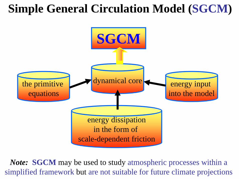
Simple General Circulation Model (SGCM)

dynamical core

SGCM

energy input into the model

the primitive equations

energy dissipationin the form of

scale-dependent friction

Note: SGCM may be used to study atmospheric processes within a simplified framework but are not suitable for future climate projections

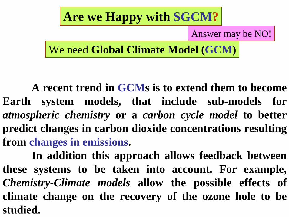
Are we Happy with SGCM?Answer may be NO!

We need Global Climate Model (GCM)

A recent trend in GCMs is to extend them to become Earth system models, that include sub-models for atmospheric chemistry or a carbon cycle model to better predict changes in carbon dioxide concentrations resulting from changes in emissions.

In addition this approach allows feedback between these systems to be taken into account. For example, Chemistry-Climate models allow the possible effects of climate change on the recovery of the ozone hole to be studied.

Global Climate Model (GCM)

physical laws (newtonian motion) empirical means

Integration fromall equations

Global Climate Model or General Circulation Model

fluid-dynamical chemical biological

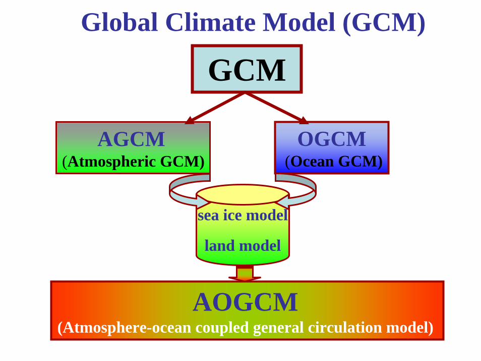
Global Climate Model (GCM)

GCM

AGCM(Atmospheric GCM)

OGCM(Ocean GCM)

AOGCM(Atmosphere-ocean coupled general circulation model)

sea ice model

land model

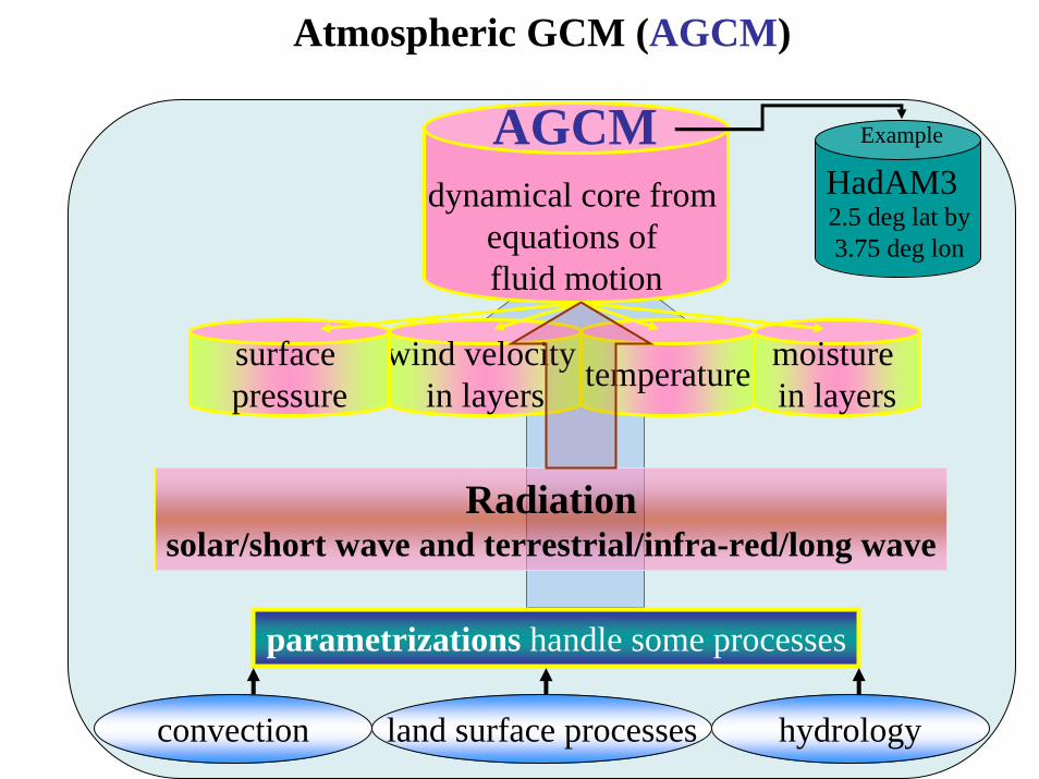
Atmospheric GCM (AGCM)

land surface processesconvection hydrology

parametrizations handle some processes

Radiationsolar/short wave and terrestrial/infra-red/long wave

moisture in layerstemperaturewind velocity

in layerssurface pressure

dynamical core from equations of fluid motion

AGCMHadAM3

Example

2.5 deg lat by3.75 deg lon

Atmosphere general circulation models (AGCMs)AGCMs consist of a three-dimensional representation of the atmosphere coupled to the land surface and cryosphere. The AGCM has to be provided with data for sea-surface temperatures and sea-ice coverage. Hence an AGCM by itself cannot be used for climate prediction, because it cannot indicate how conditions over the ocean will change. AGCMs are useful for studying atmospheric processes, the variability of climate and its response to changes in sea-surface temperature.

AGCMs coupled to a 'slab' oceanThis type of model predicts changes in sea-surface temperatures and sea ice by treating the ocean as though it were a layer of water of constant depth (typically 50 m), heat transports within the ocean being specified and remaining constant while climate changes. This kind of model is useful for simulating what the climate would be like for some fixed level of carbon dioxide, but it cannot be used for predicting the rate of change of climate because this is largely determined by processes in the ocean interior.

Atmospheric chemistry modelsThe Hadley Centre has developed a three-dimensional global atmospheric chemistry model called STOCHEM. The chemical scheme is designed to include the main agents responsible for the production and destruction of ozone and methane in the lower atmosphere.

AGCM

Model features

The first generation atmospheric general circulation model evolved from an earlier 5-layer model (Boer and McFarlane,1979). The basic structure of the model is similar to that of the spectral forecast model of Daley et al. (1976), although some improvements have been made in the procedure for implementing the spectral algorithms and of course important additional physical processes have been included. The equation governing horizontal motion are written in terms of vorticity and divergence of the horizontal wind. The remaining basic prognostic equations include the thermodynamic equation written in terms of a function of geopotential height, the moisture equation written in terms of dew-point depression, and the surface pressure equation. Temperature is determined diagnostically from the geopotentialvia the hydrostatic equation, and the vertical motion variable is determined from the mass continuity equation.

AGCM


Boundary conditionsWhile initial conditions are unimportant for general circulation models, boundary conditions have an important effect on the simulated climate. The effect of large-scale topography on the simulated climate enters into the equations of motion through the specification of the geopotential height at the surface. Surface temperatures are computed over land and oceanic pack-ice by solving the surface energy balance equation. The parameterization of surface fluxes over land requires the specification of bulk transfer coefficients at neutral stability. The drag coefficient field is used for this purpose following Cressman (1960). Surface albedo over land has a prognostic component that depends on snow cover. Background values of albedo over land, ocean and pack-ice obtained from Posey and Clapp (1964) are used.

Radiative transfer processesSolar and terrestrial radiation provides the primary energy source and sink for the climate system. In the atmospheric general circulation model described here the specification of ocean surface temperatures implies that the fluxes of heat and moisture from the oceans do not depend directly on the radiative balance of the ocean surface. Thus the model is not sensitive to the radiative calculations as it would be if an interactive ocean were present. The radiative processes that are included in the model result in heating or cooling in each atmospheric layer and at the surface which may be land or pack-ice. The radiative calculations are performed for two broad spectral regions - solar and thermal.

Horizontal transfer processesMajor horizontal transfers in the atmosphere are accomplished by the large-scale flow, which is explicitly calculated in the model. Nevertheless, the effect of unresolved horizontal scales of motion on those that are explicitly resolved in the model must be included in the formation if the results are to be realistic. While a complex physical system like the atmosphere cannot be expected to display exactly a simple turbulent behaviour, the approximate correspondence suggests that, in the absence of complete knowledge and theory concerning atmospheric behaviour, the turbulences concepts may provide useful guidance in parameterizing the effects of subgrid-scale processes on scales explicitly resolved in the model.

Precipitation and latent heat releaseIn the model, precipitation occurs and latent heat is released when the local relative humidity becomes large enough so that supersaturation can occur in a given atmospheric column. The latent heat release may be associated with moist convection when the atmosphere is locally conditionally unstable. Both condensation and convection are treated by a convective adjustment scheme and applied to individual atmospheric columns. All condensed liquid water falls to the surface as precipitation.

AGCM


Surface energy balance and hydrologyIn the model the surface of the earth may be bare or snow-covered soil, glacial or sea ice, or open ocean. Surface temperatures are specified as a function of time over the open ocean. In all other cases surface temperatures are determined so as to satisfy the requirements of a surface heat balance. The soil is considered to be completely snow covered when the snow mass per unit area exceeds a certain specified value. Surface albedo is allowed to depend on snow cover. Soil wetness and snow mass are prognostic variables in the model. Over pack-ice, snow is evaporated first but afterward the pack itself acts as an infinite reservoir of frozen water for evaporation. Gloacial ice-packs such as those over Greenland and Antarctic subcontinent are represented as thick snow layers for surface hydrology calculations. Since the solar forcing for the simulation includes annual and diurnal variations, these snow layers never melt away. Runoff is not explicitly calculated. When the total soil moisture reaches a value in excess of the field capacity the excess is assumed to run off and soil moisture is reset to unity. When rain falls on pack-ice it is assumed to run off immediately.

AGCM


Vertical discretizationThe vertical discretization of the prognostic equations in AGCM2 differs from that in AGCM1. A hybrid vertical coordinate and a finite-element formulation (both discussed in Laprise and Girard, 1990) are used in the vertical discretization of the prognostic equations in AGCM. This formulation has a number of advantages over the vertical finite-difference scheme used in AGCM2 rather than in AGCM1, including flexibility in the choice of different layering schemes for thermodynamic and momentum variables and the conservation of energy and angular momentum in the absence of physical sources or sinks. AGCM2 has ten vertical levels and employs a triangular spectral truncation having 32 longitudinal waves (T32/L10).


AGCM

Moisture variableSpecific humidity is the prognostic moisture variable in AGCM2, while dewpointdepression is used in AGCM1. This change of moisture variable was motivated mainly by the desire to ensure that the discretized prognostic equation for moisture is conservative in the absence of sources and sinks of water vapour. Such a conservation principle cannot be assured when dewpoint depression is used as the moisture variable.

Parameterization of unresolved transfer processes, precipitation, and latent heat releaseRepresentation of the effects of unresolved transfer processes and the generation of precipitation and latent heat release in AGCM2 are similar in many respects to those used in AGCM1. The moist convective adjustment and large-scale precipitation algorithms are the same as those employed in AGCM1. However, the parameterization of vertical transfer processes at the surface and in the free atmosphere have been modified to some extent.


AGCM

Turbulent vertical fluxes at the surface and in the free atmosphereVertical fluxes of momentum, heat and moisture due to turbulent transfer processes are represented using eddy diffusivity formulations in the free atmosphere, while those at the surface are represented in terms of drag coefficient formulations..

Estimation of the temperature at screen level To depict the effect of warming due to increased amounts of CO2, it is common to use either the temperature at the lowest model level or the surface temperature. These two temperature are usually different from each other, and neither is consistently more representative of the air temperature near the surface. The observed variable is, of course, the temperature at the screen level (2 m above the surface). The version of AGCM2 used for control and doubled CO2 experiments has 10 levels in the vertical with the lowest prognostic level located at approximately 200 m above the surface. AGCM2 uses a gradient profile relationship to estimate the air temperature at the screen level. The required gradient profile is obtained by noting that, in accordance with surface-layer theory, the vertical heat flux is not a function of height in the region between the surface and the screen level. In this region the diffusive representation used in the free atmosphere and the bulk formulation used at the surface are consistent with each other.


AGCM

Orographic gravity-wave dragIn particular, the effects of breaking and dissipation of unresolved orographicallyexcited gravity waves is represented as an additional drag force on the resolved flow.

Surface energy balance and hydrology over landThe treatment of surface processes over land has been modified extensively in AGCM2. A single soil-layer is used as in AGCM1, but the properties of this layer now vary with location. In order to obtain more realistic simulations of the diurnal variation of surface temperatures the energy storage in the soil is represented using the force-restore method rather than the thermal inertia method used in AGCM1. The land surface scheme in AGCM2 does not explicitly model the vegetation canopy. However, some of the effects of a vegetative canopy are represented in an approximate way by assigning spatially variable soil depths and evapotranspirationslope factors, with values being specified for each vegetation class.


AGCM

Clouds and radiation

Cloud coverageIn AGCM2 an interactive cloud scheme replaces the prescribed clouds of AGCM1. The optical properties of the clouds are also interactive variables. The fractional cloud cover is evaluated from the prognostic moisture and temperature fields through relative humidity.

Cloud optical propertiesThe optical properties of clouds are evaluated from the cloud liquid water content (LWC). In the current version the LWC is specified to be proportional to the adiabatic liquid water content that results when saturated air at ambient temperature is lifted vertically through a small distance. Cloud albedo is calculated using the delta-Eddington method (Joseph et al., 1976).


AGCM

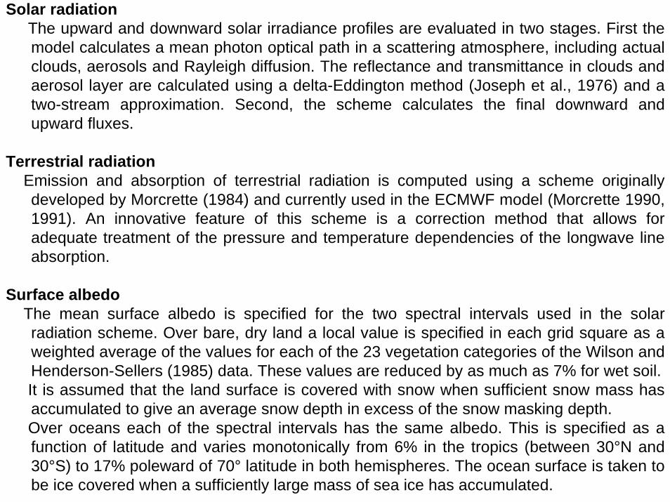
Solar radiationThe upward and downward solar irradiance profiles are evaluated in two stages. First the model calculates a mean photon optical path in a scattering atmosphere, including actual clouds, aerosols and Rayleigh diffusion. The reflectance and transmittance in clouds and aerosol layer are calculated using a delta-Eddington method (Joseph et al., 1976) and a two-stream approximation. Second, the scheme calculates the final downward and upward fluxes.

Terrestrial radiationEmission and absorption of terrestrial radiation is computed using a scheme originally developed by Morcrette (1984) and currently used in the ECMWF model (Morcrette 1990, 1991). An innovative feature of this scheme is a correction method that allows for adequate treatment of the pressure and temperature dependencies of the longwave line absorption.

Surface albedoThe mean surface albedo is specified for the two spectral intervals used in the solar radiation scheme. Over bare, dry land a local value is specified in each grid square as a weighted average of the values for each of the 23 vegetation categories of the Wilson and Henderson-Sellers (1985) data. These values are reduced by as much as 7% for wet soil. It is assumed that the land surface is covered with snow when sufficient snow mass has accumulated to give an average snow depth in excess of the snow masking depth. Over oceans each of the spectral intervals has the same albedo. This is specified as a function of latitude and varies monotonically from 6% in the tropics (between 30°N and 30°S) to 17% poleward of 70° latitude in both hemispheres. The ocean surface is taken to be ice covered when a sufficiently large mass of sea ice has accumulated.

Ocean GCM (OGCM)


HadOM3

1.25 deg mesh20 vertical layers

no sea ice model

withsea ice model

with fluxes from the atmosphere

imposed

OGCMExample

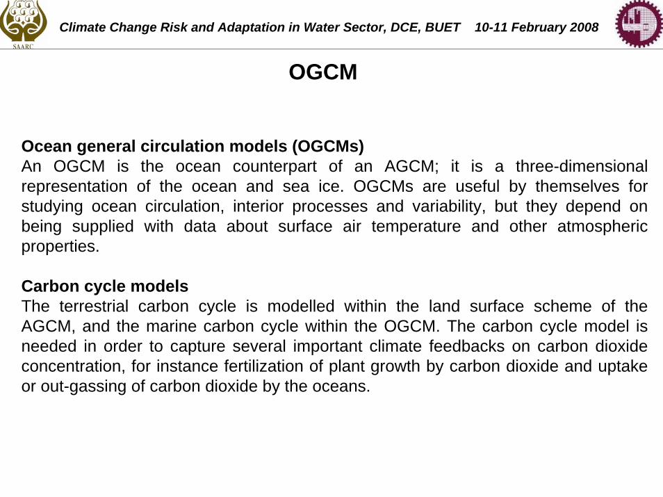
Ocean general circulation models (OGCMs)An OGCM is the ocean counterpart of an AGCM; it is a three-dimensional representation of the ocean and sea ice. OGCMs are useful by themselves for studying ocean circulation, interior processes and variability, but they depend on being supplied with data about surface air temperature and other atmospheric properties.

Carbon cycle modelsThe terrestrial carbon cycle is modelled within the land surface scheme of the AGCM, and the marine carbon cycle within the OGCM. The carbon cycle model is needed in order to capture several important climate feedbacks on carbon dioxide concentration, for instance fertilization of plant growth by carbon dioxide and uptake or out-gassing of carbon dioxide by the oceans.

OGCM


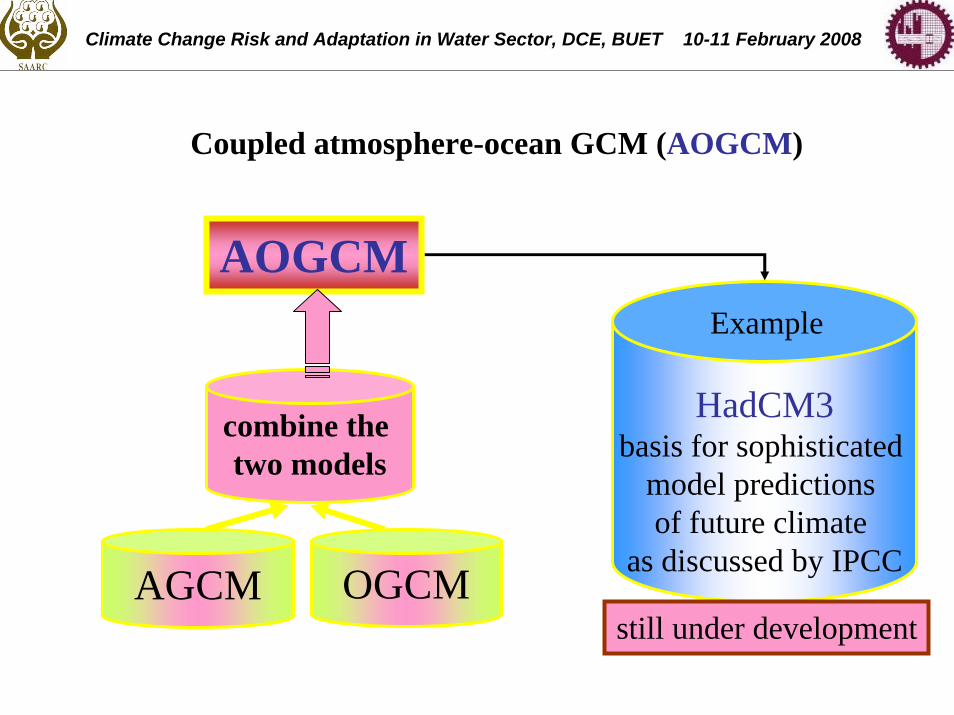
Coupled atmosphere-ocean GCM (AOGCM)


HadCM3basis for sophisticated

model predictions of future climate

as discussed by IPCC

Example

still under developmentOGCMAGCM

combine the two models

AOGCM


F. George

Coupled atmosphere-ocean general circulation models (AOGCMs) AOGCMs are the most complex models in use, consisting of an AGCM coupled to an OGCM. Some recent models include the biosphere, carbon cycle and atmospheric chemistry as well. AOGCMs can be used for the prediction and rate of change of future climate. They are also used to study the variability and physical processes of the coupled climate system. Global climate models typically have a resolution of a few hundred kilometres. Climate projections from the Hadley Centre make use of the HadCM2 AOGCM (1994) and HadCM3 AOGCM (1998). Greenhouse-gas experiments with AOGCMs have usually been driven by specifying atmospheric concentrations of the gases, but if a carbon cycle model is included, the AOGCM can predict changes in carbon dioxide concentration, given the emissions of carbon dioxide into the atmosphere. At the Hadley Centre, this was first done in 1999. Similarly, an AOGCM coupled to an atmospheric chemistry model is able to predict the changes in concentration of other atmospheric constituents in response to climate change and to the changing emissions of various gases.

AOGCM


The Third Generation Coupled Global Climate Model (CGCM3)The third version of the Canadian Centre for Climate Modelling and Analysis (CCCma) Coupled Global Climate Model (CGCM3), makes use of the same ocean component as that used in the earlier CGCM2, but it makes use of the substantially updated atmospheric component AGCM3. The sea-ice component is a two-category model (mean thickness and concentration) with cavitating fluid dynamics (Flato and Hibler, 1992) and thermodynamics as in CGCM1 and CGCM2, except that a prognostic equation for ice concentration is included following Hibler (1979). The initial version of CGCM3 was developed and ran on a NEC SX/6 vector supercomputer. A subsequent version, CGCM3.1, incorporates changes required to run efficiently on a new distributed memory IBM computer system. This latter version is the one used to produce an extensive suite of model simulations for use in the IPCC Fourth Assessment Report. CGCM3.1 is run at two different resolutions. The T47 version has a surface grid whose spatial resolution is roughly 3.75 degrees lat/lon and 31 levels in the vertical. The ocean grid shares the same land mask as the atmosphere, but has four ocean grid cells underlying every atmospheric grid cell. The ocean resolution in this case is roughly 1.85 degrees, with 29 levels in the vertical. The T63 version has a surface grid whose spatial resolution is roughly 2.8 degrees lat/lon and 31 levels in the vertical. As before the ocean grid shares the same land mask as the atmosphere, but in this case there are 6 ocean grids underlying every atmospheric grid cell. The ocean resolution is therefore approximately 1.4 degrees in longitude and 0.94 degrees in latitude.

CGCMClimate Change Risk and Adaptation in Water Sector, DCE, BUET 10-11 February 2008

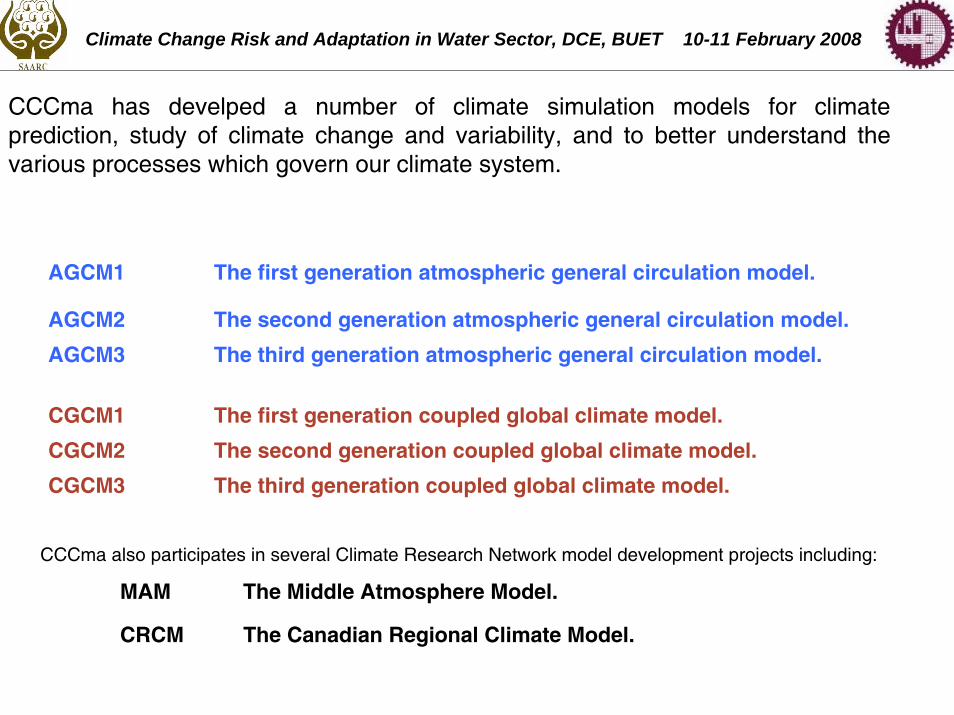
CCCma has develped a number of climate simulation models for climate prediction, study of climate change and variability, and to better understand the various processes which govern our climate system.

AGCM1 The first generation atmospheric general circulation model.

AGCM2 The second generation atmospheric general circulation model.

AGCM3 The third generation atmospheric general circulation model.

CGCM1 The first generation coupled global climate model.

CGCM2 The second generation coupled global climate model.

CGCM3 The third generation coupled global climate model.

CCCma also participates in several Climate Research Network model development projects including:


MAM The Middle Atmosphere Model.

CRCM The Canadian Regional Climate Model.

Figure : Global annual average surface temperature change, relative to 1900-1929 average as produced by CGCM1 and CGCM2 for various forcing scenarios.


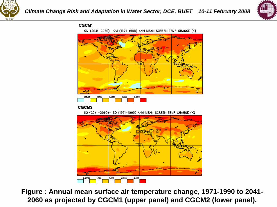
Figure : Annual mean surface air temperature change, 1971-1990 to 2041-2060 as projected by CGCM1 (upper panel) and CGCM2 (lower panel).


AGCM Model Grids


Typical AGCM resolution is between 1 and 5 deg meshand each grid point has

4 variables (u,v,T,Q)

finite difference method or the somewhat harder to

understand spectral method

AGCM

Grids

HadAM3

2.5 deg lat by3.75 deg lon

19 vertical levels

HadGEM1

1.25 deg mesh

Examples

Is it possible to provide a range of dynamical and statistical downscaling tools together with recommendations and guidanceregarding their use in order to encompass the needs of different impacts sectors for probabilistic high-resolution regional climate scenarios?

Can the best and most robust present-day state-of-art statistical downscaling methodologies be modified for integration into the ensemble prediction system?

Which, if any, of these sources of uncertainty have been reduced as a result of the ENSEMBLES work & which could be reduced with further work?

Answer may be Regional Climate Models

(RCMs)

Regional Climate ModelsThere are now 8 RCMs from 6 groups:

RCMClimate Change Risk and Adaptation in Water Sector, DCE, BUET 10-11 February 2008

ECPC RSM

IRI RSM / MM5 / REGCM2

GISS RCM

FSU FSU spectral model

NCEP ETACPTEC ETA

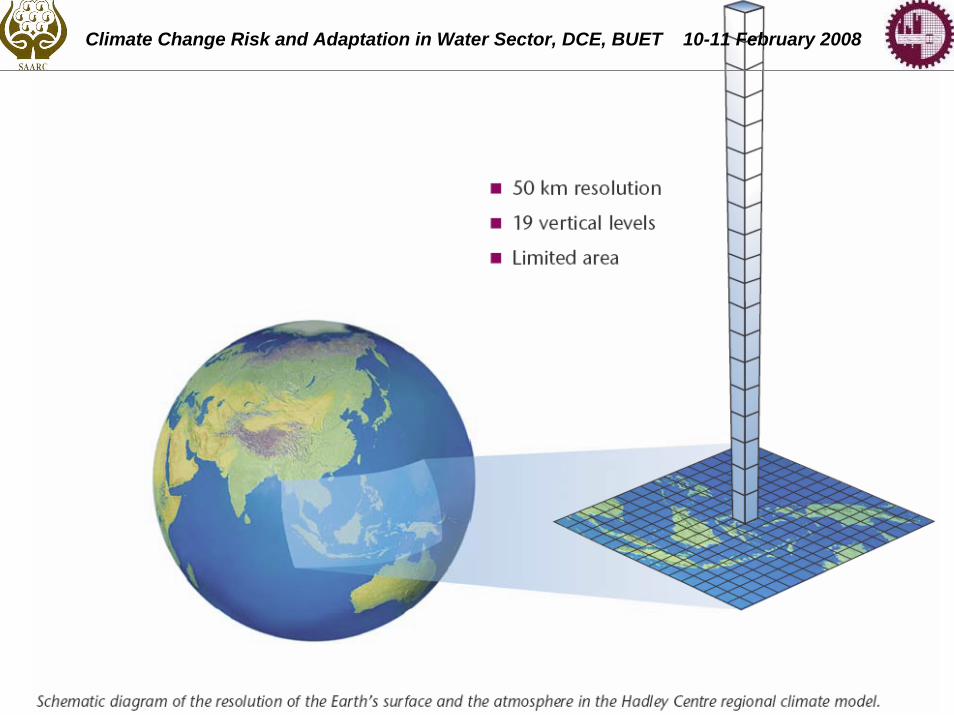
Regional climate models (RCMs)

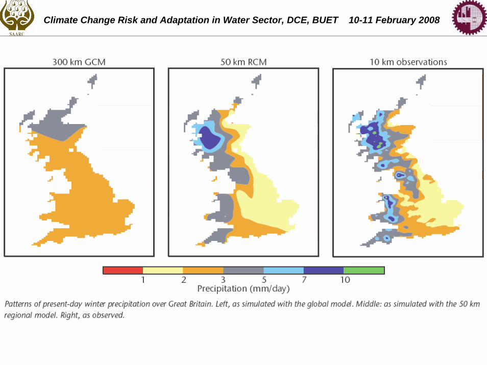
Local climate change is influenced greatly by local features such as mountains, which are not well represented in global models because of their coarse resolution. Models of higher resolution cannot practically be used for global simulation of long periods of time. To overcome this, regional climate models, with a higher resolution (typically 50 km) are constructed for limited areas and run for shorter periods (20 years or so). RCMs take their input at their boundaries and for sea-surface conditions from the global AOGCMs.

The RCM ApproachThe one-way nesting of limited area models (LAMs), suitably designed as Regional Climate Models (RCMs), within General Circulation Models (GCMs) is becoming a valuable downscaling technique for simulating the climate of a limited domain. They allow physically based and computationally affordable long-term integrations at high spatial resolution. RCMs are now been used in many climate research centres around the world.

RCM


Dynamical core (Laprise et al., 1997)Fully elastic nonhydrostatic Euler equations.

Semi-implicit semi-Lagrangian: time filter (developed by Robert (1966) and analyzed by Asselin (1972)) and uncentring of semi-implicit scheme.

3-D staggered grid: Gal-Chen terrain-following vertical-coordinate (Gal-Chen and Sommerville, 1975) along with Polar-stereographic horizontal projection.

One-way nesting over the regional domain (limited area) with lateral boundary conditions following Davies (1976) and refined by Yakimiw and Robert (1990):

-Horizontal winds U & V, air temperature, water vapour and pressure from the nesting model are imposed at the lateral boundary grid-points exactly, as interpolated onto the RCM's atmospheric levels.

-Atmospheric horizontal winds U & V relaxed toward values of the driving data over the sponge zone (generally 9 grid points).

RCM


Nesting StrategyA spectral nudging technique can be applied within the regional domain to keep the RCM's large-scale flow close to that of the driving data (Riette and Caya, 2002). The wavenumber of the smallest features passed to the nudging is user-defined, as well as the nudging intensity, which can vary according to height.

Physical parameterization

Radiative transfersSolar: improved method with three bands in the near-infrared region and one band in the visible (replacing an earlier two-band parameterization) (Puckrin et al., 2004) @ 1-h interval

Terrestrial: improved treatment of the broadband emissivities and of the water vapour continuum (Puckrin et al., 2004) @ 6-h interval Note: radiative effects of greenhouse gases are now considered separately for CO2, CH4, N2O, CFC11 and CFC12 (replacing equivalent CO2).

Vertical fluxes: heat, momentum and water vapour, turbulent eddy diffusion and surface fluxes revised turbulent transfer coefficients were introduced for surface exchanges of heat, moisture and momentum in line with AGCM3 (Abdella and McFarlane, 1996).

Gravity-wave drag: McFarlane (1987).

RCMClimate Change Risk and Adaptation in Water Sector, DCE, BUET 10-11 February 2008

Physics adapted to finer resolution:Choice of mesoscale convection scheme: Bechtold et al. (2001) or Kain and Fritsch (1990). Cloud cover onset dependent on local relative humidity and newly introduced dependence on static stability (from previous version 3.6) (Lorant et al., 2002).

Lake model:A mixed-layer/thermodynamic-ice lake model for the Laurentian Great Lakes (Goyette et al., 2000) was coupled to the CRCM. It simulates the evolution of surface water temperature and ice cover, with mixed-layer depth that can vary spatially.

Land-surface scheme : CLASS 2.7 (Canadian LAnd Surface Scheme; Verseghy, 1991; Verseghy et al., 1993) : Starting from the surface, CLASS uses three soil layers with thicknesses of 0.1 m, 0.25m and 3.75 m, corresponding approximately to the depth influenced by the diurnal cycle, the rooting zone and the annual variations of temperature, respectively.

RCM


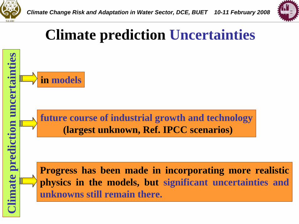
Climate prediction Uncertainties


Progress has been made in incorporating more realistic physics in the models, but significant uncertainties and unknowns still remain there.

Clim

ate

pred

ictio

n un

cert

aint

ies

in models

future course of industrial growth and technology(largest unknown, Ref. IPCC scenarios)

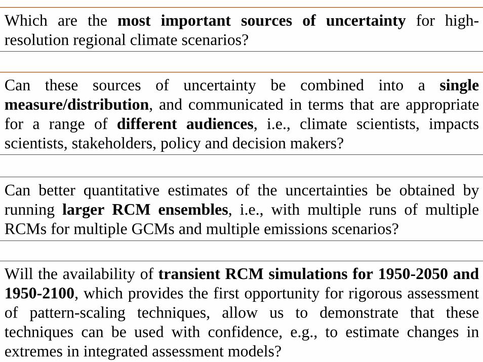
Which are the most important sources of uncertainty for high-resolution regional climate scenarios?

Can these sources of uncertainty be combined into a single measure/distribution, and communicated in terms that are appropriate for a range of different audiences, i.e., climate scientists, impacts scientists, stakeholders, policy and decision makers?

Can better quantitative estimates of the uncertainties be obtained by running larger RCM ensembles, i.e., with multiple runs of multiple RCMs for multiple GCMs and multiple emissions scenarios?

Will the availability of transient RCM simulations for 1950-2050 and 1950-2100, which provides the first opportunity for rigorous assessment of pattern-scaling techniques, allow us to demonstrate that these techniques can be used with confidence, e.g., to estimate changes in extremes in integrated assessment models?

How will impact-relevant climate parameters and meteorological extreme events such as heavy precipitation, drought, wind storms and heat waves change in the future and how do the projected changes compare with the range of natural variability?

Can more reliable high-resolution regional climate scenarios be constructed by increasing RCM resolution from 50 km to 20 km?

Answer may be PRECIS ! RegCM!Different model has different advantages.

RCMs PRECIS (Providing Regional Climate Impact Studies) and RegCM (Regional Climate Model) will be discussed in this workshop in detail.

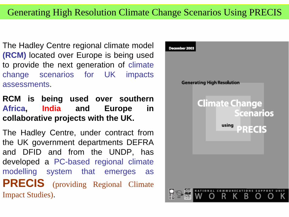
Generating High Resolution Climate Change Scenarios Using PRECIS

The Hadley Centre regional climate model (RCM) located over Europe is being used to provide the next generation of climate change scenarios for UK impacts assessments.

RCM is being used over southern Africa, India and Europe in collaborative projects with the UK.

The Hadley Centre, under contract from the UK government departments DEFRA and DFID and from the UNDP, has developed a PC-based regional climate modelling system that emerges as PRECIS (providing Regional Climate Impact Studies).

New Region PeriodScenario

Diagnostics

Run PRECIS

Stop PRECIS

PRECIS

Start 1979/12/1 Run for 1 Years

9 Months 8 Days

Hourly and daily surface and upper air data plus

climate meaning

Output format PP

Assimilated ECMWF

reanalysis abxaqNo Sulphur

All Regions

Edit Land Sea Mask

PRECIS Output format

Output data from PRECIS can be written in three different formats

PP (the UK Met Office's own data format)

NetCDF

GRIB

PP format data can be reformatted into either NetCDF or GRIB data at any point, but the reverse is not possible. This can then be converted later into NetCDF or GRIB and can be read by GrADS.

Note: GrADS does not recognize rotated coordinates as standard

We have to convert all PRECIS output in real coordinate to make useful in GrADS



Why we need PRECIS?

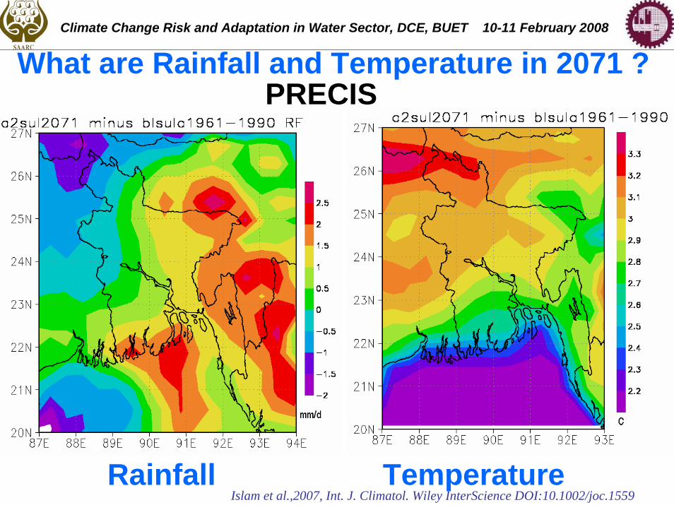
What are Rainfall and Temperature in 2071 ?PRECIS

Rainfall TemperatureIslam et al.,2007, Int. J. Climatol. Wiley InterScience DOI:10.1002/joc.1559



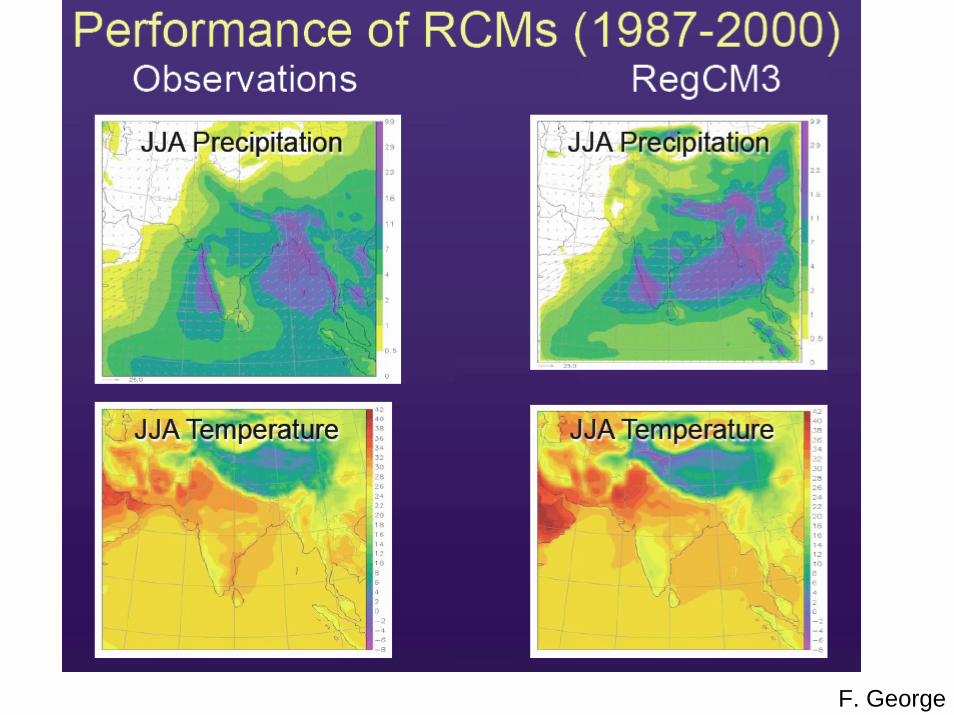
Reasons to TRUST on Simulation

88 89 90 91 9220.6

21.6

22.6

23.6

24.6

25.6

26.6

LONGITUDE (E)

LATI

TUD

E (N

)

PRECIS Rainfall JJAS 1961-90

mm/d6.577.588.599.51010.51111.51212.51313.51414.51515.516

88 89 90 91 9220.6

21.6

22.6

23.6

24.6

25.6

26.6

LONGITUDE (E)

LATI

TUD

E (N

)

Observed Rainfall JJAS 1961-90

5

6

7

8

9

10

11

12

13

14

15

16

17

18

19

20

21

mm/d

MODEL OBSERVATION

0

5

10

15

20

25

30

35

Jan

Feb

Mar

Apr

May Ju

n

Jul

Aug

Sep Oct

Nov

Dec

Tem

pera

ture

(C)

Obs Temp_1961-1990

blsula Temp_1961-1990

Islam et al.,2007, Int. J. Climatol. Wiley InterScience DOI:10.1002/joc.1559

PRECIS TEMPERATURE



Why we need RegCM?

F. George

0

2

4

6

8

10

12

14

16

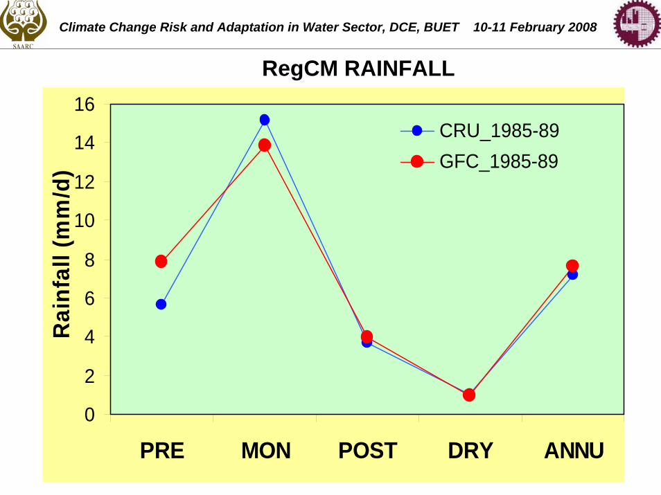
PRE MON POST DRY ANNU

Rai

nfal

l (m

m/d

)

CRU_1985-89GFC_1985-89

RegCM RAINFALL


24

25

26

27

1985 1986 1987 1988 1989

Tem

pera

ture

(C)

Kuo CRU

RegCM Annual

RegCM TemperatureClimate Change Risk and Adaptation in Water Sector, DCE, BUET 10-11 February 2008

Simulation of Killer Cyclone on 29 APRIL 1991Climate Change Risk and Adaptation in Water Sector, DCE, BUET 10-11 February 2008

CALIBRATION

SCENARIOS

GCM

LOO

K-U

P TA

BLE

APP

LIC

ATI

ONR

CMDriving

Force

PRECIS

RegCM

MM5

CReSS

Agriculture

Water Management

Fisheries

Ecology

Forestry

Infrastructure

Biodiversity

Health

Food & Disaster

Climate

2090 ?2090 ?

2080 ?

Models are ready to GENERATE future scenarios

Waiting for the demand from ENDUSERS

Grid Size ?50 km x 50 km

25 km x 25 kmMore high resolution is also possible

2070 ?2060 ?

2050 ?2040 ?

2030 ?2020 ?

2010 ?


2100 ?

Acknowledgements: All sources used in this presentation

climate change risk and adaptation in water sector, dce...

Documents