clocks, dbms and states in t imed systems
TRANSCRIPT

Clocks, DBMs and States in Timed Systems
Johan Bengtsson
A Dissertation submittedfor the Degree of Doctor of PhilosophyDepartment of Information Technology
Uppsala University
June 2002

Dissertation for the Degree of Doctor of Philosophy in Computer science withspecialization in Real Time Systems presented at Uppsala University in 2002.
ABSTRACT
Bengtsson, J. 2002: Clocks, DBMs and States in Timed Systems. Acta Universitatis UpsaliensisUppsala Dissertations from the Faculty of Science and Technology 39. 143 pp. Uppsala. ISBN91-554-5350-3
Today, computers are used to control various technical systems in our society. In manycases, time plays a crucial role in the operation of computers embedded in such systems. Thisthesis is about techniques and tools for the analysis of timing behaviours of computer systems.Its main contributions are in the development and implementation of UPPAAL, a tool designedto automate the analysis process of systems modelled as timed automata.
As the first contribution, we present a software package for timing constraints represented asDifference Bound Matrices. We describe in details, all data-structures and operations for DBMsneeded in state-space exploration of timed automata, as well as techniques for efficient imple-mentation. In particular, we have developed two normalisation algorithms to guarantee termina-tion of reachability analysis for timed automata containing constraints on clock differences, thattransform DBMs according to not only maximal constants of clocks as in algorithms publishedin the literature, but also difference constraints appearing in the automata. The second contribu-tion of this thesis is a collection of low level optimisations on the internal data-structures andalgorithms of UPPAAL to minimise memory and time consumption. We present compressiontechniques to allow the state-space of a system to be efficiently stored and manipulated in mainmemory. We also study super-trace and hash-compaction methods for timed automata to dealwith system-models for which the size of available memory is too small to store the exploredstate-space. Our experiments show that these techniques have greatly improved the performanceof UPPAAL. The third contribution is in partial-order reduction techniques for timed-systems.A major problem in automatic verification is the large number of redundant states and transi-tions introduced by modelling concurrent events as interleaved transitions. We propose a notionof committed locations for timed automata. Committed locations are annotations that can beused for not only modelling of intermediate states within atomic transitions, but also guidingthe model checker to ignore unnecessary interleavings in state-space exploration. The notion ofcommitted locations has been generalised to give a local-time semantics for networks of timedautomata, which allows for the application of existing partial order reduction techniques to timedsystems.
Johan Bengtsson, Department of Information Technology, Uppsala University, Box 337,SE-751 05 Uppsala, Sweden.
c Johan Bengtsson 2002
ISSN 1104-2516ISBN 91-554-5350-3Printed in Sweden by Elanders Gotab, Stockholm 2002Distributor: Uppsala University Library, Box 510, SE-751 20 Uppsala, Sweden

Till Erika och Simon


Acknowledgements
First of all I want to thank my supervisor, Wang Yi. Without his guiding andsupport this thesis would never have been completed. I have learnt a lot dur-ing the years we have been working together and I hope that someday I willbe as good a reasearcher as he is. I would like to thank all current and formermembers of the UPPAAL group here in Uppsala, i.e. Tobias Amnell, AlexandeDavid, Elena Fersman, Fredrik Larsson, Leonid Mokrushin, Paul Pettersson,and Justin Pearson, for the stimulating environment and all nice moments bothin and outside the department. Specially I would like to thank Fredrik and Paulwho were around from the very beginning of the UPPAAL-project. I would alsolike to thank Kim G. Larsen, Gerd Behrmann, and the rest of the UPPAAL groupin Aalborg for fruitful collaboration over the years. Without their participationUPPAAL would not have been what it is today. I am also grateful to my co-authors, i.e. Pedro D’Argenio, Ansgar Fehnker, David Griffioen, Bengt Johns-son and Johan Lilius, for fruitful discussions. It has been fun working togetherwith you.
I would like to thank everyone at DoCS for making the department such anenjoyable environment. In particular I would like to thank Björn Victor andAnders Berglund for their support.
To my wife Erika, I give my love and my deepest thanks. Without her by myside I would never have reached this point. Finally, I want to thank my sonSimon, my pride and joy, and my best source of inspiration.
This work has been partially supported by the Swedish Board for Technical Devel-opment (NUTEK), the Swedish Technical Research Council (TFR), and EC via theAIT-WOODDES project.


This thesis includes, summarises and discusses mainly the results presented infive research papers written between 1996 and 2002. These papers are listed asfollows:
Paper A: Johan Bengtsson. DBM: Structures, Operations and Implementa-tion. Submitted for publication.
Paper B: Johan Bengtsson and Wang Yi. Reachability Analysis of Timed Au-tomata Containing Constraints on Clock Differences. Submitted for pub-lication.
Paper C: Johan Bengtsson and Wang Yi. Reducing Memory Usage in Sym-bolic State-Space Exploration for Timed Systems. Technical Report, 2001-009, Department of Information Technology, Uppsala University, 2001.
Paper D: Johan Bengtsson, Bengt Jonsson, Johan Lilius and Wang Yi. Par-tial Order Reductions for Timed Systems. In Proceedings, Ninth Inter-national Conference on Concurrency Theory, volume 1466 of LectureNotes in Computer Science, Springer Verlag, 1998.
Paper E: Johan Bengtsson, W. O. David Griffioen, Kåre J. Kristoffersen, Kim G.Larsen, Fredrik Larsson, Paul Pettersson and Wang Yi. Automated Veri-fication of an Audio-Control Protocol using UPPAAL. Accepted for pub-lication in Journal on Logic and Algebraic Programming.
Comments on My Participation
Paper A: I implemented the major part of the DBM package in UPPAAL, andwrote the report.
Paper B: I participated in discussions, designed and implemented the algo-rithms. I wrote a large part of the paper.
Paper C: I participated in discussions, designed and implemented the optimi-sation techniques. I wrote the paper.
Paper D: I participated in discussions and wrote part of the paper. I made aprototype implementation which is not described in this paper.
Paper E: I participated in discussions and implemented committed locationsin UPPAAL. I have also made minor revisions to the semantics for com-mitted location.

Apart from the papers listed above, I have also participated in the followingwork:
Tobias Amnell, Gerd Behrmann, Johan Bengtsson, Pedro R. D’Argenio, Alexan-dre David, Ansgar Fehnker, Thomas Hune, Bertrand Jeannet, Kim G. Larsen, M.Oliver Möller, Paul Pettersson, Carsten Weise, and Wang Yi. UPPAAL - Now,Next, and Future. In Proceedings of Modelling and Verification of Parallel Pro-cesses, volume 2067 of LNCS, 2001.
Johan Bengtsson, Kim G. Larsen, Fredrik Larsson, Paul Pettersson, Wang Yiand Carsten Weise. New Generation of UPPAAL. In Proceedings of the Inter-national Workshop on Software Tools for Technology Transfer, 1998
Johan Bengtsson, Kim G. Larsen, Fredrik Larsson, Paul Pettersson, Wang Yi.UPPAAL in 1995, In Proceedings of Workshop on Tools and Algorithms for theConstruction and Analysis of Systems, volume 1055 of LNCS, 1996.
Johan Bengtsson, Kim G. Larsen, Fredrik Larsson, Paul Pettersson and WangYi. UPPAAL - a Tool Suite for Automatic Verification of Real-Time Systems.In Proceedings of Workshop on Verification and Control of Hybrid Systems III,volume 1066 of LNCS, 1995.

Contents
Introduction 1
1 Background . . . . . . . . . . . . . . . . . . . . . . . . . . . 1
2 Timed Automata . . . . . . . . . . . . . . . . . . . . . . . . 2
3 Model Checking . . . . . . . . . . . . . . . . . . . . . . . . . 7
4 Contributions of This Thesis . . . . . . . . . . . . . . . . . . 9
5 Related Work . . . . . . . . . . . . . . . . . . . . . . . . . . 12
6 Conclusions and Future Work . . . . . . . . . . . . . . . . . . 15
Paper A: DBM: Structures, Operations and Implementation 23
1 Introduction . . . . . . . . . . . . . . . . . . . . . . . . . . . 25
2 DBM basics . . . . . . . . . . . . . . . . . . . . . . . . . . . 26
2.1 Canonical DBMs . . . . . . . . . . . . . . . . . . . . 27
2.2 Minimal Constraint Systems . . . . . . . . . . . . . . 28
3 Operations on DBMs . . . . . . . . . . . . . . . . . . . . . . 31
3.1 Checking Properties of DBMs . . . . . . . . . . . . . 33
3.2 Transformations . . . . . . . . . . . . . . . . . . . . 33
3.3 Normalisation Operations . . . . . . . . . . . . . . . 36
4 Zones in Memory . . . . . . . . . . . . . . . . . . . . . . . . 38
4.1 Storing DBM Elements . . . . . . . . . . . . . . . . . 38
i

4.2 Placing DBMs in Memory . . . . . . . . . . . . . . . 39
4.3 Storing Sparse Zones . . . . . . . . . . . . . . . . . . 39
5 Conclusions . . . . . . . . . . . . . . . . . . . . . . . . . . . 40
A Pseudo-Code . . . . . . . . . . . . . . . . . . . . . . . . . . 42
Paper B: Reachability Analysis of Timed Automata Containing Con-straints on Clock Differences 45
1 Introduction . . . . . . . . . . . . . . . . . . . . . . . . . . . 47
2 Preliminaries . . . . . . . . . . . . . . . . . . . . . . . . . . 50
2.1 Timed Automata Model . . . . . . . . . . . . . . . . 50
2.2 Reachability Analysis . . . . . . . . . . . . . . . . . 51
3 Constraints on Clock Differences and Normalisation . . . . . 53
4 New Normalisation Algorithms . . . . . . . . . . . . . . . . . 54
4.1 Region Equivalence Refined by Difference Constraints 56
4.2 The Core of Normalisation . . . . . . . . . . . . . . . 56
4.3 Algorithm: Normalisation without Zone Splitting . . . 57
4.4 Algorithm: Normalisation with Zone Splitting . . . . . 58
5 Conclusion . . . . . . . . . . . . . . . . . . . . . . . . . . . 63
Paper C: Reducing Memory Usage in Symbolic State-Space Explo-ration for Timed Systems 67
1 Introduction . . . . . . . . . . . . . . . . . . . . . . . . . . . 69
2 Preliminaries . . . . . . . . . . . . . . . . . . . . . . . . . . 70
3 Representing Symbolic States . . . . . . . . . . . . . . . . . 73
3.1 Normal Representation . . . . . . . . . . . . . . . . . 73
3.2 Packed States . . . . . . . . . . . . . . . . . . . . . . 74
3.3 Packed Zones with Cheap Inclusion Check . . . . . . 75
4 Representing the Symbolic State-Space . . . . . . . . . . . . 78
ii

4.1 Representing WAIT . . . . . . . . . . . . . . . . . . . 78
4.2 Representing PASSED . . . . . . . . . . . . . . . . . 80
4.3 Supertrace PASSED for Timed Automata . . . . . . . 80
4.4 Hash Compaction for Timed Automata . . . . . . . . 83
5 Conclusions . . . . . . . . . . . . . . . . . . . . . . . . . . . 86
A Examples and Experiment Environment . . . . . . . . . . . . 91
Paper D: Partial Order Reductions for Timed Systems 93
1 Motivation . . . . . . . . . . . . . . . . . . . . . . . . . . . . 95
2 Preliminaries . . . . . . . . . . . . . . . . . . . . . . . . . . 99
2.1 Networks of Timed Automata . . . . . . . . . . . . . 99
2.2 Symbolic Global–Time Semantics . . . . . . . . . . . 100
3 Partial Order Reduction and Local-Time Semantics . . . . . . 102
3.1 Symbolic Local-Time Semantics . . . . . . . . . . . . 104
3.2 Finiteness of the Symbolic Local Time Semantics . . . 106
4 Partial Order Reduction in Reachability Analysis . . . . . . . 108
4.1 Operations on Constraint Systems . . . . . . . . . . . 110
5 Conclusion and Related Work . . . . . . . . . . . . . . . . . 111
Paper E: Automated Verification of an Audio-Control Protocol usingUPPAAL 115
1 Introduction . . . . . . . . . . . . . . . . . . . . . . . . . . . 117
2 Committed Locations . . . . . . . . . . . . . . . . . . . . . . 119
2.1 An Example . . . . . . . . . . . . . . . . . . . . . . 120
2.2 Syntax . . . . . . . . . . . . . . . . . . . . . . . . . 121
2.3 Semantics . . . . . . . . . . . . . . . . . . . . . . . . 122
3 Committed Locations in UPPAAL . . . . . . . . . . . . . . . 124
3.1 The Model-Checking Algorithm . . . . . . . . . . . . 124
iii

3.2 Space and Time Performance Improvements . . . . . 127
4 The Audio Control Protocol with Bus Collision . . . . . . . . 128
5 A Formal Model of the Protocol . . . . . . . . . . . . . . . . 130
6 Verification in UPPAAL . . . . . . . . . . . . . . . . . . . . . 133
7 Conclusions . . . . . . . . . . . . . . . . . . . . . . . . . . . 135
8 Appendix . . . . . . . . . . . . . . . . . . . . . . . . . . . . 139
iv

Introduction 1
Introduction
1 Background
The computer boom in the last decades has not only given us faster and moreadvanced equipment for word-processing, banking and scientific computations.The development of small, cheap, and powerful microprocessors has also en-abled a range of new application areas. Today, computers are trusted to controlall kinds of devices and technical systems used in our society, ranging fromstereos and micro-wave ovens to life-support systems and nuclear power-plants.Currently this kind of computer applications, i.e. the embedded systems, formsthe fastest growing market for microprocessors. In recent years 98%–99% ofall produced processors have been used in embedded systems [Hal00]. Onlyaround 2% are used in desktop computers.
In many embedded applications, a computer failure may have dire consequences,such as economical damage, environmental catastrophes and even loss of hu-man lives. Thus it is of great importance that such systems operate correctly,according to their specifications. Traditionally this is accomplished by methodslike reviewing of design documents and source code and by extensive simu-lation and testing of the system and its components. However, this process isoften time-consuming and provides only statistical measures of correctness.
As a complement to the traditional methods for obtaining correct software, alarge number of mathematically based techniques for reasoning about correct-ness of computer systems have been proposed in the literature, e.g. [Hoa69,Dij75, Hoa78, Rei85, Mil89, Hol91]. The common procedure in all these socalled formal methods is to define the system under development in a formalframework and then apply rigorous methods within this framework to provethat the system meets its requirements. However, due to the complexity of real-life systems, applying formal methods is often considered too difficult. A way
2 Introduction
to bridge this gap is to automate the analysis, for instance by using model-checking [CGP99]. In contrast to manual techniques, model-checking is fullyautomatic in the sense that the proof showing that a system satisfies a givenrequirement is constructed by the model-checker without manual interaction.
In this thesis we study and develop techniques for model-checking tools to ver-ify systems where timing is important. The work presented in this thesis is inthe context of the model-checker UPPAAL, which is a tool for analysing timingproperties of systems modelled as timed automata.
2 Timed Automata
Timed automata [AD90, AD94, HNSY94] is one of the most successful for-malisms for describing the timing behaviour of computer systems. Examples ofother formal systems with the same purpose, are timed Petri-net models, timedprocess algebras or real time logics [BD91, RR88, Yi91, NS94, ACD93, AH94,SS95].
A Brief Introduction to Timed Automata
A timed automaton is essentially a finite automaton extended by a set of realvalued clocks. All clocks are synchronised in the sense that they start with thevalue zero when the system is initialised and grow synchronously, with the samerate. The clocks influence the automaton by clock-constraints (guards) on theedges. An edge is only enabled when the values of the clocks satisfies the guard.The automaton can influence the clocks by letting the edges reset a subset ofthe clocks.
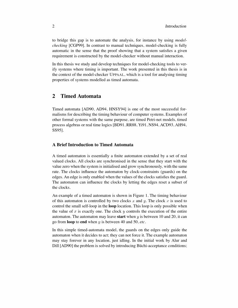
An example of a timed automaton is shown in Figure 1. The timing behaviourof this automaton is controlled by two clocks and . The clock is used tocontrol the small self-loop in the loop location. This loop is only possible whenthe value of is exactly one. The clock controls the execution of the entireautomaton. The automaton may leave start when is between 10 and 20, it cango from loop to end when is between 40 and 50, etc.
In this simple timed-automata model, the guards on the edges only guide theautomaton when it decides to act; they can not force it. The example automatonmay stay forever in any location, just idling. In the initial work by Alur andDill [AD90] the problem is solved by introducing Büchi-acceptance conditions;

Introduction 3
start
loop
end
x:=0, y:=0
10<=y<=20enter
40<=y<=50
y:=0leave
x==1
x:=0work 10<=y<=20
y:=0
Figure 1: A Timed Automaton
a subset of the locations in the automaton are marked as accepting, and onlyexecutions passing through an accepting location infinitely often are consideredvalid. As an example, consider again the automaton in Figure 1 and assume thatend is marked as accepting. This implies that all executions of the system enterend infinitely many times. This impose implicit conditions on start and loop.The location start must be left when the value of is at most 20, otherwisethe automaton would get stuck and never be able to enter end. Likewise, theautomaton must leave loop when is at most 50 to be able to enter end.
Büchi-acceptance conditions are theoretically elegant. However, as the exam-ple shows, an accepting location has global effects on the automaton, which isinconvenient for modelling and automatic analysis. A more intuitive notion ofprogress is used in timed safety-automata [HNSY94]. In timed safety-automata,the acceptance conditions are replaced by local timing constraints in each loca-tion, that is the so called location invariants. The automaton may only remainin a location as long as the clocks satisfies the invariant condition. This givesa more convenient view of the timing behaviour of particular parts of the au-tomaton. For example, consider the automaton in Figure 2. This timed safety-automaton corresponds to the Büchi automaton in the previous example. In thisautomaton the conditions that start and end must be left when is at most 20and loop must be left when is at most 50 are now stated locally in invariants.This gives a local view of the timing in each location in much more convenientway than Büchi-acceptance. For this reason we will use timed automata withlocation invariants to describe the timing behaviour of embedded systems.
To model concurrent systems, timed automata is often extended with parallelcomposition, giving networks of timed automata. In the early work on timed-automata [AD90, HNSY92], parallel composition is treated as logical con-

4 Introduction
starty<=20
loopy<=50
endy<=20
x:=0, y:=0
10<=yenter
40<=y
y:=0leave
x==1
x:=0work 10<=y
y:=0
Figure 2: A Timed Safety-Automaton
junction, i.e. all processes in a system must synchronise on every action. Inthis thesis, as well as in UPPAAL, we adopt the parallel composition usedin CCS [Mil89], which allows for internal actions in processes, as well aspair-wise synchronisation. An example of a system composed of two timed-automata is presented in Figure 3. The network models a time-dependent light-switch (to the left) and its user (to the right). The user and the switch com-municate by the press labels. The user can press the switch (press!) and theswitch waits to be pressed (press?). The product automaton, i.e. the automatondescribing the combined system is shown in Figure 4. Building the product au-tomaton is an entirely syntactical operation based on the component automata.In UPPAAL, the product automaton is computed on-the-fly during verification.
off
dim
bright
press?x:=0
x<=10press?
x>10press?
press?
ty<5
study
idle
relax
press!y:=0 press!
y>10
press!y:=0
press!
press!
Figure 3: Network of Timed Automata

Introduction 5
off,idle dim,relax
dim,t
y<5
bright, study
off,study
bright,t
y<5
dim,idle
bright,relax dim,study
off,t
y<5
bright, idle
off,relax
x:=0, y:=0
x>10, y>10
x:=0, y:=0
x<=10
x>10
x:=0
x<=10 y:=0
x<10y:=0
x>10
x>10 y:=0
x>10
x<=10,y>10
x<=10
y:=0
x>10y:=0
y>10x:=0
y:=0
Figure 4: Product Automaton for the Network in Figure 3
Semantics of Timed Automata
A state or configuration of a timed automaton has two different parts, the currentlocation and the current values of all clocks. There are two different types oftransitions between states. The automaton may either delay for some time (a de-lay transition), or follow an enabled edge (an action transition). Since clocks ina timed automaton are real-valued the state-space will be infinite and not a goodbase for automatic verification. However, many verification problems such aslanguage emptiness, reachability analysis and model-checking of timed logicscan still be decided by constructing a region graph based on the automaton un-der consideration and perform the analysis on this graph [AD94, ACD93]. Thedownside with this solution is the large number of states in the region-graph. Asan example, consider Figure 5. The figure shows the possible regions in eachlocation of an automaton with two clocks and . The largest number com-pared to is 3, and the largest number compared to is 2. In the figure eachline segment, each intersection and each area is one region. Thus, the numberof possible regions in each location of this example is 60. It also grows rapidlywith the number of clocks and the largest constants. In fact, the region graphis exponential in the number of clocks in the system as well as the in largestconstants appearing in guards in the automaton.

6 Introduction
y
x
Figure 5: Regions for a System with Two Clocks
A more appealing representation of the state-space for timed automata is ob-tained by using zone-graphs [Dil89, HNSY94, ACH 95]. Instead of regions,the clock values are represented as constraints on clocks and clock differences.In practice this gives a coarser and thus more compact representation of thestate space. The basic operations and algorithms to construct zone-graphs aredescribed in Paper A. As an example, a timed automaton and the correspondingzone graph is shown in Figure 6. We note that for this automaton the zone graphhas only eight states. The region-graph for the same example has over fifty.
off
dim
bright
press?x:=0
x<=10press?
x>10press?
press?
off
off
off
dim
dimbright
bright
bright
Figure 6: A Timed Automaton and the corresponding Zone Graph
The zone-graph of a timed automaton may unfortunately be infinite and ver-ification based on zone-graphs is thus not guaranteed to terminate. As an ex-ample, consider the model in Figure 7. In this automaton the value of clockdrifts away unboundedly, giving an infinite graph. The solution is to normalisethe zones in the zone-graph with respect to the maximum constants in the au-tomaton, that is the so called -normalisation [Rok93, Pet99]. The intuition isthat once the value of a clock is larger than the maximum constant in the au-

Introduction 7
tomaton it is no longer significant for the automaton to know its precise value,only that it is above the constant. As an example, the -normalised zone-graphof the automaton in Figure 7 is given in Figure 8. Note that the -normalisationonly works for timed automata with guards on individual clocks. For automatawith guards on clock differences a more elaborate normalisation procedure isneeded (see Paper B).
start
loopx<=10
end
x:=0,y:=0
x>=20x:=0,y:=0
x==10x:=0
start
loop
loop
loop
loop
end...
Figure 7: A Timed Automaton with an Infinite Zone Graph
start
loop
loop
loop
loop
end
Figure 8: Normalised Zone Graph for the Automaton in Figure 7
3 Model Checking
Model-checking consists of two steps, computing the state-space of the systemunder consideration, and searching for states, or sets of states that satisfy cer-tain logical properties. The first step can either be performed prior to the search,

8 Introduction
or done on-the-fly during the search process. Computing the state-space on-the-fly has an obvious advantage over pre-computing, in that only the part of thestate-space needed to prove (or disprove) the property is generated. As an ex-ample, consider a system with a million states. Generating the full state-spaceof this system will take a lot of time and may even be infeasible due to memoryrequirements. However, if the logical properties of interests can be proven byonly examining the first hundred states of the system then an on-the-fly methodwill only need to generate those states and the result will be almost instanta-neous. It should be noted though, that even on-the-fly methods will generatethe entire state-space to prove certain properties, e.g. invariant properties.
The model-checking procedure itself is based on traversing the state-space insearch for states that prove or contradict stated logical properties. As an exam-ple, we use one of the model-checking algorithms for timed-automata imple-mented in UPPAAL (see Algorithm 1).
Algorithm 1 Reachability analysisPASSED WAITwhile WAIT do
take from WAITif then return “YES”if for all PASSED then
add to PASSEDfor all such that do
add to WAITend for
end ifend whilereturn “NO”
The algorithm is used for verifying safety properties (that something bad willnever happen) for networks of timed automata. The properties are given to thealgorithm as a set of bad states ( denotes a location in the networkand denotes a clock zone). The algorithm will then compute the zone-graphof the system on-the-fly, in search for states intersecting with . The al-gorithm highlights some of the issues in developing a model-checker for timedautomata. First, handling of states, or primarily zones, is crucial to the per-formance of the model-checker. Thus, devising algorithms and data-structuresfor zones is a major issue in developing a verification tool for timed automata,which is addressed in Paper A. Second, PASSED holds all states encountered so

Introduction 9
far and its size puts a limit on how large systems we can verify. This makes itimportant to find compact representations for PASSED. However, since passedis searched each time a new state is processed it is crucial to performance thatsearching is cheap. This leads to a tradeoff between size and speed. We studythis problem in Paper C.
A major obstacle in constructing the state-space of a network of timed automatais the so called state-explosion problem. The problem appears in all kinds ofmodel-checkers, and the source of the problem is the practice of modellingconcurrent systems using parallel composition of several automata. The effectis a rapid growth of the explored state-space due to the fact that each possibleinterleaving of the automata will be taken into account by the analysis.
A method for reducing the state-space used in model-checkers for untimed sys-tems is partial-order reductions. With this technique the state-space is reducedby removing interleavings of independent transitions and choose one represen-tative. However, in timed-automata the number of independent transitions ismuch less than in the untimed case due to the tight synchronisation of time.One way of breaking this synchronisation, without affecting stated reachabilityproperties, is presented in Paper D.
Finally we shall point out that a powerful verification engine is not enough toget a successful tool and there are other issues in building verification tools. Fora tool to be widely used it requires substantial work on the user interface. Forinstance, in UPPAAL a lot of effort has been put on improving the user interface.However, such issues are not the topic of this thesis.
4 Contributions of This Thesis
The main contributions of this thesis are in the development and implemen-tation of UPPAAL, a tool-suite for timed-automata developed in collaborationbetween Uppsala University and Aalborg University. The first version of UP-PAAL was released in spring 1995, and was then the first verification tool fortimed automata where the system model could be drawn graphically (WhatYou See Is What You Verify). In 1996, another step was taken in the samedirection, when UPPAAL was equipped with a simulator that enable the userto test system models interactively and to visualise counterexamples generatedby the model-checker. In 1999, the architecture of UPPAAL was completelychanged, the tool was separated into two parts: A graphical user interface anda verification engine. Among other things this change enabled the GUI and the

10 Introduction
verification engine to be run on separate machines, e.g. running the GUI on alocal work-station and the verification engine on a large server. Today UPPAALis one of the most popular tools for timed automata and it has been downloadedby over 1300 different users from over 70 countries.
The performance of the verification engine has always been a key issue whendeveloping UPPAAL. This is also the part where most of the contributions de-scribed in this thesis are located.
A DBM Package: Data-Structures and Operations [Paper A,B]
Zones are the most important entities in a model-checker for timed systems andtheir representation and implementation are crucial to the performance. In im-plementing UPPAAL we discovered a number of techniques to improve perfor-mance of zone operations. In this thesis we present our experiences in form ofa cook-book on Difference Bound Matrices [Dil89]. We describe all primitiveoperations and data-structures for zones needed to implement state-space ex-ploration for time-automata in both forwards and backwards analysis, includingoperations for checking properties of zones, for computing the effect of delay-ing and resetting of clocks, and for constraining a zone with respect to a guard.We also present how to normalise the clock-zones with respect to guards in theautomaton to guarantee that the model-checking procedure terminates. In par-ticular we discovered that the existing -normalisation algorithms published inthe literature do not work for timed-automata with guards on clock-differences.We have developed two new normalisation algorithms for automata that maycontain constraints on clock differences.
Low-Level Optimisations [Paper C]
The performance of UPPAAL has been greatly improved by low-level optimi-sations on its central algorithms and data-structures. In this thesis we developand evaluate a number of techniques to minimise memory and time consump-tion. The techniques are implemented in UPPAAL and we believe that they aregeneric and applicable to model-checking of timed-systems in general.
We present two different methods for packing states. First, we code the entirestate as one large number using a multiply-and-add algorithm. This methodyields a representation that is canonical and minimal in terms of memory usagebut the performance for inclusion checking between states is poor. The secondmethod is mainly intended to use for the timing part of the state and it is basedon concatenation of bit strings. Using a special concatenation of the bit string

Introduction 11
representation of the constraints in a zone, ideas from [PS80] can be used toimplement fast inclusion checking between packed zones.
The problem representing large state-spaces is addressed in two different ways.First, to get rid of states that do not need to be explored, as early as possible,we introduce inclusion checking already in the data structure keeping the stateswaiting to be explored. We also describe an implementation where time, aswell as memory, is saved by this technique. Second, we investigate how super-trace [Hol91] and hash-compaction [WL93, SD95b] methods can be applied totimed systems. We present a variant of the hash compaction method, that allowstermination of branches in the search tree based on probable inclusion checkingbetween states. These techniques have been implemented in the UPPAAL tool,evaluated and compared by real-life examples; their strengths and weaknessesare described.
Partial Order Reduction [Paper D,E]
A major problem in automatic verification is the large number of states intro-duced by modelling concurrent events as interleaved transitions. In many cases,the order of the transitions are irrelevant for the investigated properties and onespecific order can be chosen to represent all. In this thesis we address this prob-lem in a setting of timed systems. We present a notion of committed locationsfor timed automata. Committed locations are annotations that can be used fornot only modelling of intermediate states within atomic transitions, but alsoguiding the model checker to ignore unnecessary interleavings in state-spaceexploration. During modelling, intermediate locations in sequences of internalactions can be marked as committed. This prohibits delay in the locations andallows its transitions to be interleaved only with transitions of committed lo-cations in other automata in the network. We present a modified algorithm forstate space exploration for networks of timed automata which generate a re-duced number of states when committed locations are used. Our experimentalresults demonstrate significant time and space-savings for a number of applica-tions. For example, the audio control protocol presented in Paper E could nothave been verified in 1995 without using committed locations.
Committed location is a simple case of getting rid of unnecessary interleavingsin sequences of transitions without delays. Naturally, we want to extend thenotion to sequences with non-zero delays. However, due to the tight synchro-nisation of time, delay in timed-automata has a global effect. To resolve thisissue, we introduce a notion of local-time and let local clocks in each processadvance independently of clocks in other processes. To avoid communication
12 Introduction
between processes with different notion of the current time we require pro-cesses to resynchronise their local time scales whenever they communicate. Asymbolic local-time semantics is developed in terms of predicate transformers,which enjoys the desired property that two predicate transformers are inde-pendent if they correspond to disjoint transitions in different processes. Thisallows existing partial order reduction techniques to be applied to the problemof reachability analysis for timed systems.
5 Related Work
In the past years, a large number of model-checkers have been developed by re-searchers for different application areas. For examples, we mention SPIN [Hol91,Hol97] for communication protocols and Mur [DDHY92] for concurrent andreactive systems, UPPAAL [LPY97, ABB 01] and KRONOS [DOTY95, Yov97,BDM 98] for timed systems, and HYTECH [HHWT97] for hybrid systems.These tools have all been successfully applied to industrial-size case studies,e.g. [HLP98, JMMS98, SD95a, MMS97, LPY98, HSLL97, TY98, HWT96].In this section we summarise the most successful and known techniques imple-mented in these tools.
Partial-order reduction: Partial-order methods [God90, Val90, Pel93] are bas-ed on the observation that in many cases the exact ordering of events affectsneither the examined properties nor how the system evolves in the future. Inthese cases all equivalent orderings can be represented by one single ordering.For timed-automata there are two different approaches to applying partial orderreductions. The first approach was introduced by Pagani in [Pag96] and laterimproved by Dams et. al. [DGKK98]. It is based on the global-time semanticsof timed automata. This limits the possible reductions in that only transitionsthat can occur in exactly the same time-interval can be independent. The sec-ond approach is the local-time approach proposed in Paper D of this thesis.In [Min99], Minea extends our result for reachability analysis to LTL model-checking. Minea also shows that standard normalisation techniques for timing-constraints are applicable also in local-time semantics.
Symmetry reductions: Symmetry reduction [HJJJ84, ID96, ES97] is a methodfor exploiting the fact that many system-models have a large number of iden-tical processes. It is often the case that these identical processes may be in-terchanged without noticeably affecting the system. As an example, in a com-munication protocol it may not matter if process A is sending and process B

Introduction 13
is receiving or the other way around. In a model-checker this is exploited bydefining equivalence classes for states based on different permutations of theidentical processes. The model-checking algorithm is then applied to the graphof equivalence classes instead of the full state-space. As examples. we men-tion that this technique has been implemented in the tools Mur [ID96] andSGM [HW98, WH02].
Symbolic model-checking: The key idea of symbolic model-checking is inrepresenting and manipulating sets of states in terms of logical formulae. Thebest known symbolic technique, introduced in [BCM 92], describe states andtransitions as propositional formulae and use BDDs [Bry86] to store and manip-ulate them. The so called bounded model-checking is introduced in [BCCZ99].In this work, the task of checking if a system-model has a certain logical prop-erty is transformed into checking satisfiability for a series of propositional for-mulae. Symbolic techniques for timed-systems are all based on zones [Dil89,HNSY94, AHH96, ACH 95, YPD94], where sets of clock-values are repre-sented and manipulated using clock constraints. This is the main topic of thisthesis.
Approximation methods: Approximation methods are aimed at systems thatare too large to be handled by precise methods, at the price that some results areinconclusive. There are two different types of approximation methods, under-approximations where part of the reachable state-space may be considered notreachable by the model-checker, and over-approximations where non-reachablestates may be considered reachable by algorithm. Two examples of under-approximation are Supertrace [Hol91] and hash-compaction [WL93, SD95b].These methods may conclude erroneously during verification that some unex-plored state has been visited before. Thus, with under-approximations, a claimthat invariant properties hold is inconclusive, since states violating the propertymay be lost in the approximation. Over-approximation techniques are oftencombined with symbolic model-checking. Often, the union of two symbolic-states can not be precisely represented by a single formula while it is possibleto construct a formula including two symbolic states. In [Bal96] this type ofmethod is applied to verification of timed automata. In the paper the convex-hull of time-zones are used as an approximation of union. In [WT94], Wong-Toipresents techniques for refining the results obtained by over-approximations bycombining the results from forwards and backwards analysis.
Efficient Representation of Clock Constraints: In a verification tool, a largefraction of memory used during verification is spent on storing clock con-straints. In the literature there are a number of techniques addressing this prob-

14 Introduction
lem. In [DY96] live-range analysis is used to reduce the number of clocks ina model. The control-structure of the system-model is analysed to compute theset of active clocks for each location. To save space, only timing information re-garding active clocks are stored. Another approach is taken in [LLPY97]. Thiswork is based on the observation that the DBM representation of a time zoneoften contains redundant information, i.e. the same set of clock values can berepresented using much fewer constraints. The paper presents an algorithm forcomputing the minimal set of constraints for a given DBM.
Inspired by the success of using BDDs to encode state-spaces in hardware ver-ification, a number of similar techniques for representing clock zones weredeveloped. In [Bal96], Balarin present a schema for encoding DBMs usingDBBs. He also develop algorithms for performing essential DBM operationsdirectly on the BDD. In [ABK 97], Asarin et. al. introduce Numerical Deci-sion Diagrams (NDDs), a technique for representing sets of regions from theregion-graph of timed automata as BDDs. The problem with both these repre-sentations is their sensitivity to time-granularity. This problem is not presentfor Clock Difference Diagrams (CDDs) [LPWY99, BLP 99] and DifferenceDecision Diagrams (DDDs) [MLAH99a, MLAH99b], which are two similartypes of decision diagrams based on difference constraints. They allow for non-convex unions of zones to be represented by a single diagram, and the maindifference is that in DDDs each node represents a single difference constraint,while a node in a CDD represents all difference constraints on a clock-pair.Thus, DDDs will, in general, have more nodes than the corresponding CDD,while the nodes in a CDD have a larger and variable number of edges.
Low-Level Optimisations: For many applications, it is not feasible to store allexplored states in main memory. In [SD98], Stern and Dill present a methodfor storing PASSED on magnetic disk. To compensate for the increased time toaccess PASSED, they collect a large number of states in WAIT and check all ofthem in one sequential sweep through PASSED. Other alternatives when dealingwith large state-spaces is to store only enough states to guarantee termination.In [LLPY97] static analysis of the system-model is used to compute the setof loop-entry location in the processes. A state is then stored in PASSED onlyif one of the processes enter such a location. This guarantee that at least onestate in each dynamic loop will be present on PASSED and thus termination isensured. A method for throwing identifying and removing states that no longercan be revisited is presented in [CKM01]. A progress measure is used by themodel-checker to identify such states.

Introduction 15
6 Conclusions and Future Work
This thesis summarises our experiences in developing and implementing UP-PAAL. We have studied and developed techniques to improve the performanceof UPPAAL in the verification process. Our main contributions are in three di-rections. First we have presented a DBM package including all data-structuresand operations needed in symbolic state-space exploration of timed automata.We hope that the included reports may serve as a cook-book for tool develop-ers of timed-systems. Second, we have presented and implemented a collec-tion of low-level optimisations on the central algorithms and data-structures ofUPPAAL. They have given significant performance improvements for the tool.Though these techniques are developed for UPPAAL, we believe that they aregeneric and applicable to other model-checkers for timed-systems. As the thirdcontribution we have presented partial-order reduction techniques for timedsystems. The notion of committed locations has been a useful mechanism fornot only modelling atomic sequences but also guiding the model-checker toavoid redundant interleavings in state-space exploration. Though the notion ofcommitted locations has been generalised to give a local-time semantics fornetworks of timed automata, which allows for partial order reductions in state-space exploration of timed systems, the technique has not yet been fully ex-plored. This is a challenging area for future work. The local-time semantics isjust a step on the way. A challenge is to develop an efficient implementation ofthe technique.
The work presented in this thesis can be extended in several directions. Hierar-chical extensions to timed automata is a direction that is currently being pursuedwithin the UPPAAL group. A challenging problem is how to take advantage ofthe hierarchical structures in state-space exploration. As future work, we willfurther study techniques to reduce memory requirements without losing perfor-mance in time, e.g. to develop packing methods and hash functions for zones,that preserve inclusion checking.
References
[ABB 01] Tobias Amnell, Gerd Behrmann, Johan Bengtsson, Pedro R. D’Argenio,Alexandre David, Ansgar Fehnker, Thomas Hune, Bertrand Jeannet,Kim G. Larsen, M. Oliver Möller, Paul Pettersson, Carsten Weise, andWang Yi. UPPAAL - Now, Next, and Future. In Modelling and Verifica-tion of Parallel Processes, volume 2067 of Lecture Notes in ComputerScience, pages 100–125. Springer-Verlag, 2001.

16 Introduction
[ABK 97] Eugene Asarin, Marius Bozga, Alain Kerbrat, Oded Maler, Amir Pnueli,and Anne Rasse. Data structures for the verification of timed automata.In Proceedings, Hybrid and Real-Time Systems, volume 1201 of LectureNotes in Computer Science, pages 346–360. Springer-Verlag, 1997.
[ACD93] Rajeev Alur, Costas Courcoubetis, and David L. Dill. Model-checking indense real-time. Journal of Information and Computation, 104(1):2–34,1993.
[ACH 95] Rajeev Alur, Costas Courcoubetis, Nicholas Halbwachs, Thomas A.Henzinger, Pei-Hsin Ho, Xavier Nicollin, Alfredo Olivero, JosephSifakis, and Sergio Yovine. The algorithmic analysis of hybrid systems.Journal of Theoretical Computer Science, 138(1):3–34, 1995.
[AD90] Rajeev Alur and David L. Dill. Automata for modeling real-time sys-tems. In Proceedings, Seventeenth International Colloquium on Au-tomata, Languages and Programming, volume 443 of Lecture Notes inComputer Science, pages 322–335. Springer-Verlag, 1990.
[AD94] Rajeev Alur and David L. Dill. A theory of timed automata. Journal ofTheoretical Computer Science, 126(2):183–235, 1994.
[AH94] Rajeev Alur and Thomas A. Henzinger. A really temporal logic. Journalof the ACM, 41(1):181–204, 1994.
[AHH96] Rajeev Alur, Thomas A. Henzinger, and Pei-Hsin Ho. Automatic sym-bolic verification of embedded systems. IEEE Transactions on SoftwareEngineering, 22:181–201, 1996.
[Bal96] Felice Balarin. Approximate reachability analysis of timed automata. InProceedings, 17th IEEE Real-Time Systems Symposium. IEEE ComputerSociety Press, 1996.
[BCCZ99] Armin Biere, Alessandro Cimatti, Edmund M. Clarke, and Yunshan Zhu.Symbolic model checking without BDDs. In Proceedings, Fifth Inter-national Conference on Tools and Algorithms for the Construction andAnalysis of Systems, volume 1579 of Lecture Notes in Computer Science.Springer-Verlag, 1999.
[BCM 92] J. R. Burch, E. M. Clarke, K. L. McMillan, D. L. Dill, and L. J. Hwang.Symbolic model checking: states and beyond. Journal of Informa-tion and Computation, 98(2):142–170, 1992.
[BD91] Bernard Berthomieu and Michel Diaz. Modeling and verification oftimed dependent systems using timed petri nets. IEEE Transactions onSoftware Engineering, 17(3):259–273, 1991.
[BDM 98] Marius Bozga, Conrado Daws, Oded Maler, Alfredo Olivero, StavrosTripakis, and Sergio Yovine. Kronos: a model-checking tool for real-time systems. In Proceedings, Tenth International Conference on Com-puter Aided Verification, volume 1427 of Lecture Notes in Computer Sci-ence. Springer-Verlag, 1998.

Introduction 17
[BLP 99] Gerd Behrmann, Kim G. Larsen, Justin Pearson, Carsten Weise, andWang Yi. Efficient timed reachability analysis using clock difference dia-grams. In Proceedings, Eleventh International Conference on ComputerAided Verification, volume 1633 of Lecture Notes in Computer Science,pages 341–353. Springer-Verlag, 1999.
[Bry86] Randal E. Bryant. Graph-based algorithm for boolean function manipu-lation. IEEE Transactions on Computers, C-35(8):677–691, 1986.
[CGP99] Edmund M. Clarke, Orna Grumberg, and Doron A. Peled. Model Check-ing. The MIT Press, 1999.
[CKM01] Søren Christensen, Lars Michael Kristensen, and Thomas Mailund. Asweep-line method for state space exploration. In Proceedings, SeventhInternational Conference on Tools and Algorithms for the Constructionand Analysis of Systems, volume 2031 of Lecture Notes in ComputerScience, pages 450–464. Springer-Verlag, 2001.
[DDHY92] David L. Dill, Andreas J. Drexler, Alan J. Hu, and C. Han Yang. Protocolverification as a hardware design aid. InProceedings, IEEE InternationalConference on Computer Design, VLSI in Computers and Processors,pages 522–525. IEEE Computer Society Press, 1992.
[DGKK98] Dennis Dams, Rob Gerth, Bart Knaack, and Ruurd Kuiper. Partial-orderreduction techniques for real-time model checking. Formal Aspects ofComputing, 10(5–6):469–482, 1998.
[Dij75] E. W. Dijkstra. Guarded commands, nondeterminacy and formal deriva-tion of programs. Communications of the ACM, 18(8):453–457, 1975.
[Dil89] David L. Dill. Timing assumptions and verification of finite-state concur-rent systems. In Proceedings, Automatic Verification Methods for FiniteState Systems, volume 407 of Lecture Notes in Computer Science, pages197–212. Springer-Verlag, 1989.
[DOTY95] Conrado Daws, Alfredo Olivero, Stavros Tripakis, and Sergio Yovine.The tool Kronos. In Proceedings, Hybrid Systems III: Verification andControl, volume 1066 of Lecture Notes in Computer Science. Springer-Verlag, 1995.
[DY96] Conrado Daws and Sergio Yovine. Reducing the number of clock vari-ables of timed automata. In Proceedings, 17th IEEE Real-Time SystemsSymposium. IEEE Computer Society Press, 1996.
[ES97] E. Allen Emerson and A. Prasad Sistla. Using symmetry when mod-elchecking under fairness assumptions: An automata theoretic approach.ACM Transactions on Programming Languages and Systems, 19(4),1997.

18 Introduction
[God90] Patrice Godefroid. Using partial orders to improve automatic verificationmethods. In Proceedings, Second International Conference on ComputerAided Verification, volume 531 of Lecture Notes in Computer Science,pages 176–185. Springer-Verlag, 1990.
[Hal00] Tom R. Halfhill. Embedded market breaks new ground. MicroprocessorReport, January 2000.
[HHWT97] Thomas A. Henzinger, Pei-Hsin Ho, and Howard Wong-Toi. HYTECH:A model checker for hybrid systems. Journal on Software Tools forTechnology Transfer, pages 110–122, 1997.
[HJJJ84] Peter Huber, Arne M. Jensen, Leif O. Jespen, and Kurt Jensen. Towardsreachability trees for high-level petri nets. In Proceedings, Advanceson Petri Nets ’84, volume 188 of Lecture Notes in Computer Science.Springer-Verlag, 1984.
[HLP98] Klaus Havelund, Mike Lowry, and John Penix. Formal analysisof a space craft controller using Spin. In Proceedings, Fourth In-ternational SPIN Workshop, 1998. Proccedings available online.URL: http://netlib.bell-labs.com/netlib/spin/ws98/program.html.
[HNSY92] Thomas A. Henzinger, Xavier Nicollin, Joseph Sifakis, and SergioYovine. Symbolic model checking for real-time systems. In Proceed-ings, Seventh Annual IEEE Symposium on Logic in Computer Science,pages 394–406, 1992.
[HNSY94] Thomas A. Henzinger, Xavier Nicollin, Joseph Sifakis, and SergioYovine. Symbolic model checking for real-time systems. Journal ofInformation and Computation, 111(2):193–244, 1994.
[Hoa69] C. A. R. Hoare. An axiomatic basis for computer programming. Com-munications of the ACM, 12(10):576–580, 1969.
[Hoa78] C. A. R. Hoare. Communicating sequential processes. Communicationsof the ACM, 21(8):666–677, 1978.
[Hol91] Gerard J. Holzmann. Design and Validation of Computer Protocols.Prentice-Hall, 1991.
[Hol97] Gerard J. Holzmann. The model checker Spin. IEEE Transactions onSoftware Engineering, 23(5):279–295, 1997.
[HSLL97] Klaus Havelund, Arne Skou, Kim G. Larsen, and Kristian Lund. Formalmodelling and analysis of an audio/video protocol: An industrial casestudy using UPPAAL. In Proceedings, 18th IEEE Real-Time SystemsSymposium, pages 2–13. IEEE Computer Society Press, 1997.
[HW98] Pao-Ann Hsiung and Farn Wang. A state-graph manipulator tool for real-time system specification and verification. In Proceedings, Fifth Inter-national Conference on Real-Time Computing Systems and Applications,1998.
Introduction 19
[HWT96] Thomas A. Henzinger and Howard Wong-Toi. Using HYTECH to syn-thesize control parameters for a steam boiler. In Formal Methods forIndustrial Applications: Specifying and Programming the Steam BoilerControl, number 1165 in Lecture Notes in Computer Science, pages265–282. Springer-Verlag, 1996.
[ID96] C. Norris Ip and David L. Dill. Better verification through symmetry.Journal of Formal Methods in System Design, 9, 1996.
[JMMS98] Wil Janssen, Radu Mateescu, Sjouke Mauw, and Jan Springintveld.Verifying business processes using SPIN. In Proceedings, FourthInternational SPIN Workshop, 1998. Proccedings available online.URL: http://netlib.bell-labs.com/netlib/spin/ws98/program.html.
[LLPY97] Kim G. Larsen, Fredrik Larsson, Paul Pettersson, and Wang Yi. Efficientverification of real-time systems: Compact data structure and state spacereduction. In Proceedings, 18th IEEE Real-Time Systems Symposium,pages 14–24. IEEE Computer Society Press, 1997.
[LPWY99] Kim G. Larsen, Justin Pearson, Carsten Weise, and Wang Yi. Clockdifference diagrams. Nordic Journal of Computing, 1999.
[LPY97] Kim G. Larsen, Paul Petterson, and Wang Yi. UPPAAL in a nutshell.Journal on Software Tools for Technology Transfer, 1997.
[LPY98] Magnus Lindahl, Paul Pettersson, and Wang Yi. Formal Design andAnalysis of a Gear-Box Controller. In Proceedings, Fourth Workshopon Tools and Algorithms for the Construction and Analysis of Systems,number 1384 in Lecture Notes in Computer Science, pages 281–297.Springer-Verlag, 1998.
[Mil89] Robin Milner. Communication and Concurrency. Prentice Hall Interna-tional Series in Computer Science. Prentice Hall, 1989.
[Min99] Marius Minea. Partial Order for Verification of Timed Systems. PhDthesis, School of Computer Science, Carnegie Mellon University, 1999.
[MLAH99a] Jesper Møller, Jakob Lichtenberg, Henrik Reif Andersen, and HenrikHulgaard. Difference decision diagrams. In Proceedings, 13th Inter-national Workshop on Computer Science Logic, volume 1683 of LectureNotes in Computer Science. Springer-Verlag, 1999.
[MLAH99b] Jesper Møller, Jakob Lichtenberg, Henrik Reif Andersen, and HenrikHulgaard. On the symbolic verification of timed systems. TechnicalReport IT-TR-1999-024, Department of Information Technology, Tech-nical University of Denmark, 1999.
[MMS97] John C. Mitchell, Mark Mitchell, and Ulrich Stern. Automated analysisof cryptographic protocols using Mur . In Proceedings, 1997 Confer-ence on Security and Privacy, pages 141–153. IEEE Computer SocietyPress, 1997.

20 Introduction
[NS94] Xavier Nicollin and Joseph Sifakis. The algebra of timed processes,ATP: Theory and application. Journal of Information and Computation,114(1):131–178, 1994.
[Pag96] Florence Pagani. Partial orders and verification of real-time systems. InProceedings, Fourth International Symposium on Formal Techniques inReal-Time and Fault-Tolerant Systems., volume 1135 of Lecture Notesin Computer Science, pages 327–346. Springer-Verlag, 1996.
[Pel93] Doron Peled. All from one, one for all: on model checking using repre-sentatives. In Proceedings, Fifth International Conference on ComputerAided Verification, volume 697 of Lecture Notes in Computer Science,pages 409–423. Springer-Verlag, 1993.
[Pet99] Paul Pettersson. Modelling and Verification of Real-Time Systems UsingTimed Automata: Theory and Practice. PhD thesis, Uppsala University,1999.
[PS80] Wolfgang J. Paul and Janos Simon. Decision trees and random accessmachines. In Logic and Algorithmic, volume 30 of Monographie deL’Enseignement Mathématique, pages 331–340. L’Enseignement Math-ématique, Université de Genève, 1980.
[Rei85] Wolfgang Reisig. Petri nets. An Introduction. In EATCS Monographs onTheoretical Compute Science, volume 4. Springer Verlag, 1985.
[Rok93] Tomas Gerhard Rokicki. Representing and Modeling Digital Circuits.PhD thesis, Stanford University, 1993.
[RR88] G. M. Reed and A. W. Roscoe. A timed model for communicatingsequential processes. Theoretical Computer Science, 58(1-3):249–261,1988.
[SD95a] Ulrich Stern and David L. Dill. Automatic verification of the SCI cachecoherence protocol. In Correct Hardware Design and Verification Meth-ods: IFIP WG10.5 Advanced Research Working Conference Proceed-ings, 1995.
[SD95b] Ulrich Stern and David L. Dill. Improved probabilistic verification byhash compaction. In Correct Hardware Design and Verification Meth-ods: IFIP WG10.5 Advanced Research Working Conference Proceed-ings, 1995.
[SD98] Ulrich Stern and David L. Dill. Using magnetic disk instead of mainmemory in the Mur verifier. In Proceedings, Tenth International Con-ference on Computer Aided Verification, volume 1427 of Lecture Notesin Computer Science. Springer-Verlag, 1998.
[SS95] Oleg V. Sokolsky and Scott A. Smolka. Local model checking for real-time systems. In Proceedings, Seventh International Conference onComputer Aided Verification, volume 939 of Lecture Notes in ComputerScience. Springer-Verlag, 1995.

Introduction 21
[TY98] Stavros Tripakis and Sergio Yovine. Verification of the fast reservationprotocol with delayed transmission using the tool Kronos. In Proceed-ings, Fourth IEEE Real-Time Technology and Applications Symposium.IEEE Computer Society Press, 1998.
[Val90] Antti Valmari. A stubborn attack on state explosion. In Proceedings, Sec-ond International Conference on Computer Aided Verification, volume531 of Lecture Notes in Computer Science, pages 156–165. Springer-Verlag, 1990.
[WH02] Farn Wang and Pao-Ann Hsiung. Efficient and user-friendly verification.IEEE Transactions on Computers, 51(1):61–83, 2002.
[WL93] Pierre Wolper and Dennis Leroy. Reliable hashing without collision de-tection. In Proceedings, Fifth International Conference on ComputerAided Verification, volume 697 of Lecture Notes in Computer Science,pages 59–70. Springer-Verlag, 1993.
[WT94] Howard Wong-Toi. Symbolic Approximation for Verifying Real-TimeSystems. PhD thesis, Stanford University, 1994.
[Yi91] Wang Yi. CCS + time = an interleaving model for real time systems. InProceedings, Eighteenth International Colloquium on Automata, Lan-guages and Programming, volume 510 of Lecture Notes in ComputerScience. Springer-Verlag, 1991.
[Yov97] Sergio Yovine. Kronos: a verification tool for real-time systems. Journalon Software Tools for Technology Transfer, 1, October 1997.
[YPD94] Wang Yi, Paul Petterson, and Mats Daniels. Automatic verification ofreal-time communicating systems by constraint-solving. In Proceedings,Seventh International Conference on Formal Description Techniques,pages 223–238, 1994.


Paper A:DBM: Structures, Operations and Implementation
Johan Bengtsson.


DBM: Structures, Operations and Implementation 25
DBM: Structures, Operations and Implementation
Johan Bengtsson
Abstract. A key issue when building a verification tool for timed sys-tems is how to handle timing constraints arising in state-space explo-ration. Difference Bound Matrices (DBMs) is a well-studied techniquefor representing and manipulating timing constraints. The goal of thispaper is to provide a cook-book and a software package for the devel-opment of verification tools using DBMs. We present all operations onDBMs needed in symbolic state-space exploration for timed automata,as well as data-structures and techniques for efficient implementation.
1 Introduction
During the last ten years, timed automata [AD90, AD94] has evolved as a com-mon model for timed systems and one of the reasons behind its success is theavailability of verification tools, such as UPPAAL [LPY97, ABB 01] and KRO-NOS [DOTY95, Yov97], that can verify industrial-size applications modelled astimed automata. The major problem in automatic verification is the large num-ber states induced by the state explosion. For timed systems this problem hasan even larger impact since both the number of states and the size of a singlestate are significantly larger than in the untimed case due to timing constraints.This makes devising data-structures for states and timing constraints one of thekey challenges in developing verification tools for timed systems.
In this paper we describe a software package for representing timing constraints,arising from state space exploration of timed systems, as difference bound ma-trices [Dil89]. The package is based on the DBM implementation of [BL96] butit has been significantly improved using implementation experiences gainedfrom developing the current version of UPPAAL. The paper is intended as acook-book for developers of verification tools and the goal is to provide a basisfor the implementation of state-of-the-art verification tools.
The paper is organised as follows: In Section 2 we introduce the DBM struc-ture and its canonical form; we also describe how to find the minimal numberof constraints needed to represent the same set of clock assignments as a givenDBM. Section 3 lists all DBM operations needed to implement a verification

26 DBM: Structures, Operations and Implementation
tool such as UPPAAL together with efficient algorithms for these operations.Some suggestions on how to store the structures in memory are given in Sec-tion 4 and finally Section 5 concludes the paper.
2 DBM basics
The key objects for representing timing information in symbolic state-spaceexploration for timed systems are a special class of constraint systems referredto as difference-bound constraint-systems or, more commonly, zones. A zonefor a set of clocks is a conjunction of atomic constraints of the form and
where , and . What make zonesso important is their simple structure and that the set of zones is closed withrespect to the strongest postcondition of all operations needed in state-spacegeneration.
Since zones are frequently used objects, their representation is a major issuewhen building a verification tool for timed automata. In this section we describethe basic concepts behind Difference Bound Matrices (DBM) [Dil89], which isone of the most effective data structures for zones.
To have a unified form for clock constraints we introduce a reference clockwith constant value 0. Let . Then any zone can berewritten as a conjunction of constraints of the form for ,
and .
Naturally, if the rewritten zone has two constraints on the same pair of variablesonly the tightest of them is significant. Thus, a zone can be represented using atmost atomic constraints of the form such that each pair of clocks
is mentioned only once. We can then store zones using matriceswhere each element in the matrix corresponds to an atomic constraint. Sinceeach element in such a matrix represents a bound on the difference betweentwo clocks, we call them Difference Bound Matrices (DBMs). In the followingpresentation we let denote element in the DBM representing the zone
.
To compute the DBM representation for a zone , we start by numbering allclocks in to assign one row and one column in the matrix to each clock. Therow is used for storing lower bounds on the difference between the clock andall other clocks while the column is used for upper bounds. The elements in thematrix are then computed in three steps.

DBM: Structures, Operations and Implementation 27
For each bound in , in , let .
For each clock difference that is unbounded in , let .Where is a special value denoting that no bound is present.
Finally add the implicit constraints that all clocks are positive, i.e., and that the difference between a clock and itself is always 0, i.e.
.
As an example, consider the zone. To construct the matrix representation of , we
number the clocks in the order . The resulting matrix representation isshown below:
To manipulate DBMs efficiently we need two operations on bounds: compari-son and addition. We define that , ifand . Further we define addition as ,
and .
2.1 Canonical DBMs
Usually there are an infinite number of zones sharing the same solution set.However, for each family of zones with the same solution set there is a uniqueconstraint system where no atomic constraint can be strengthened without los-ing solutions. We say that such a zone is closed under entailment or just closed.Since there is a unique closed zone for each solution set we use closed zones ascanonical representation of entire families of zones.
To compute the closed representative of a given zone we need to derive thetightest constraint on each clock difference. To solve this problem, we use agraph-interpretation of zones. If we see zones as a weighted graphs where theclocks in are nodes and the atomic constraints are edges, deriving boundscorresponds to adding weights along paths in the graph. Note that DBMs formadjacency matrices for this graph-interpretation.
28 DBM: Structures, Operations and Implementation
(a) (b)
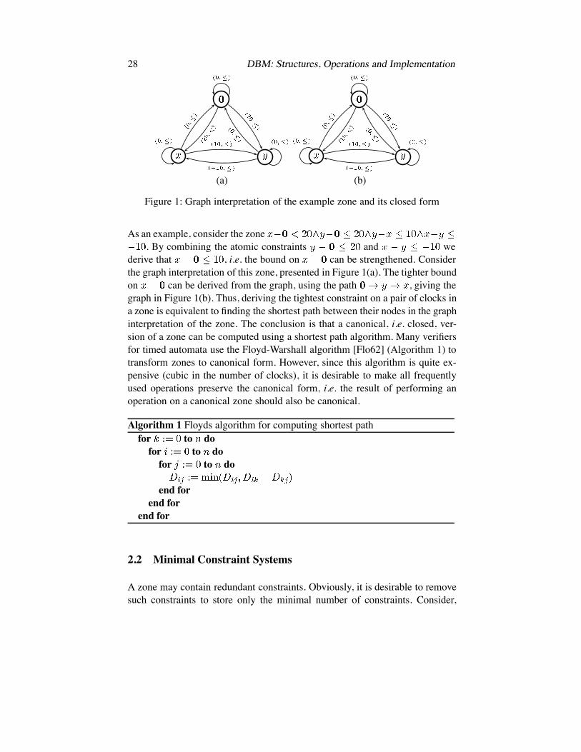
Figure 1: Graph interpretation of the example zone and its closed form
As an example, consider the zone. By combining the atomic constraints and we
derive that , i.e. the bound on can be strengthened. Considerthe graph interpretation of this zone, presented in Figure 1(a). The tighter boundon can be derived from the graph, using the path , giving thegraph in Figure 1(b). Thus, deriving the tightest constraint on a pair of clocks ina zone is equivalent to finding the shortest path between their nodes in the graphinterpretation of the zone. The conclusion is that a canonical, i.e. closed, ver-sion of a zone can be computed using a shortest path algorithm. Many verifiersfor timed automata use the Floyd-Warshall algorithm [Flo62] (Algorithm 1) totransform zones to canonical form. However, since this algorithm is quite ex-pensive (cubic in the number of clocks), it is desirable to make all frequentlyused operations preserve the canonical form, i.e. the result of performing anoperation on a canonical zone should also be canonical.
Algorithm 1 Floyds algorithm for computing shortest pathfor to do
for to dofor to do
end forend for
end for
2.2 Minimal Constraint Systems
A zone may contain redundant constraints. Obviously, it is desirable to removesuch constraints to store only the minimal number of constraints. Consider,

DBM: Structures, Operations and Implementation 29
for instance, the zone, which is in minimal form. This zone is completely defined by only five
constraints. However, the closed form contains no less than 12 constraints. Itis known, e.g. from [LLPY97], that for each zone there is a minimal constraintsystem with the same solution set. By computing this minimal form for all zonesand storing them in memory using a sparse representation we might reducethe memory consumption for state-space exploration. This problem has beenthoroughly investigated in [LLPY97, Pet99, Lar00] and this presentation is asummary of the work presented there.
The goal is to find an algorithm that computes the minimal form of a closedDBM. However, closing a DBM corresponds to computing the shortest pathbetween all clocks. Thus, we want to find an algorithm that computes the mini-mal set of bounds with a given shortest path closure. For clarity, the algorithmis presented in terms of directed weighted graphs. However, the results are di-rectly applicable to the graph interpretation of DBMs.
First we introduce some notation: we say that a cycle in a graph is a zero cycleif the sum of weights along the cycle is 0, and an edge is redundantif there is another path between and where the sum of weights is no largerthan .
In graphs without zero cycles we can remove all redundant edges without af-fecting the shortest path closure [Pet99]. Further, if the input graph is in shortestpath form (as for closed DBMs) all redundant edges can be located by consid-ering alternative paths of length two.
As an example, consider Figure 2. The figure shows the shortest path closurefor a zero-cycle free graph (a) and its minimal form (b). In the graph we findthat is made redundant by the path and can thusbe removed. Further, the edge is redundant due to
. Note that we consider edges marked as redundant when searching for newredundant edges. The reason is that we let the redundant edges represent thepath making them redundant, thus allowing all redundant edges to be locatedusing only alternative paths of length two. This procedure is repeated until nomore redundant edges can be found.
This gives the procedure for removing redundant edges presented inAlgorithm 2. The algorithm can be directly applied to zero-cycle free DBMs tocompute the minimal number of constraints needed to represent a given zone.

30 DBM: Structures, Operations and Implementation
9
8
7
5
13
126
15
13
7
2
1
7
5
6 2
1
(a) (b)
Figure 2: A zero cycle free graph and its minimal form
Algorithm 2 Reduction of Zero-Cycle Free Graph with nodesfor to do
for to dofor to do
if thenMark edge as redundant
end ifend for
end forend forRemove all edges marked as redundant.
However, this algorithm will not work if there are zero-cycles in the graph.The reason is that the set of redundant edges in a graph with zero-cycles is notunique. As an example, consider the graph in Figure 3(a). Applying the abovereasoning on this graph would remove based on the path
. It would also remove the edge based on the path .But if both these edges are removed it is no longer possible to construct pathsleading into . In this example there is a dependence between the edges
and such that only one of them can be considered redundant.
The solution to this problem is to partition the nodes according to zero-cyclesand build a super-graph where each node is a partition. The graph from Fig-ure 3(a) has two partitions, one containing and and the other containing
. To compute the edges in the super-graph we pick one representative foreach partition and let the edges between the partitions inherit the weights fromedges between the representatives. In our example, we choose and as

DBM: Structures, Operations and Implementation 31
-2
3
2
5
3
1
-2
3
2
3
(a) (b)
Figure 3: A graph with a zero-cycle and its minimal form
representatives for their equivalence classes. The edges in the graph are thenand . The super-graph is clearly zero-cycle
free and can be reduced using Algorithm 2. This small graph can not be re-duced further. The relation between the nodes within a partition is uniquelydefined by the zero-cycle and all other edges may be removed. In our exampleall edges within each equivalence class are part of the zero-cycle and thus noneof them can be removed. Finally the reduced super-graph is connected to thereduced partitions. In our example we end up with the graph in Figure 3(b).Pseudo-code for the reduction-procedure is shown in Algorithm 3.
Now we have an algorithm for computing the minimum number of edges torepresent a given shortest path closure that can be used to compute the minimumnumber of constraints needed to represent a given zone.
3 Operations on DBMs
This section presents all operations on DBMs needed in symbolic state spaceexploration of timed automata, both for forwards and backwards analysis. Notethat even if a verification tool only explores the state space in one directionall operations are still useful for other purposes, e.g. for generating diagnostictraces. The effects of the operations are shown graphically in Figure 5.
In the following section we do not distinguish between DBMs and zones, andthe terms are used alternately. To simplify the presentation we assume that theclocks in are numbered and the index for is 0. We assume that theinput zones are consistent and in canonical form.

32 DBM: Structures, Operations and Implementation
Algorithm 3 Reduction of negative-cycle free graph with nodesfor to do
if Node is not in a partition then
for to doif then
Nodeend if
end forend if
end forLet be a graph without nodes.for each do
Pick one representative NodeAdd Node toConnect Node to all nodes in using weights from .
end forReducefor each do
Add one zero cycle containing all nodes in toend for
The operations on DBMs can be divided into three different classes:
1. Property-Checking: Operations in this class include checking if a DBMis consistent, checking inclusion between zones, and checking whether azone satisfies a given atomic constraint.
2. Transformation: This is the largest class containing operations for trans-forming zones according to guards, delay and reset.
3. Normalisation: They are used to normalise zones in order to obtain afinite zone-graph. In this paper we only describe one operation in thisclass, the so called -normalisation. For more normalisation operationswe refer to [BY01].

DBM: Structures, Operations and Implementation 33
3.1 Checking Properties of DBMs
consistent( )
The most basic operation on a DBM is to check if it is consistent, i.e. if thesolution set is non-empty. In state-space exploration this operation is used toremove inconsistent states from exploration.
For a zone to be inconsistent there must be at least one pair of clocks where theupper bound on their difference is smaller than the lower bound. For DBMs thiscan be checked by searching for negative cost cycles in the graph interpretation.However, the most efficient way to implement a consistency check is to detectwhen an upper bound is set to lower value than the corresponding lower boundand mark the zone as inconsistent by setting to a negative value. For azone in canonical form this test can be performed locally. To check if a zone isinconsistent it will then be enough to check whether is negative.
relation( )
Another key operation in state space exploration is inclusion checking for thesolution sets of two zones. For DBMs in canonical form, the condition that
for all clocks is necessary and sufficient to conclude that. Naturally the opposite condition applies to checking if . This
allows for the combined inclusion check described in Algorithm 5.
satisfied( )
Sometimes it is desirable to non-destructively check if a zone satisfies a con-straint, i.e. to check if the zone is consistent without altering
. From the definition of the consistent-operation we know that a zone isconsistent if it has no negative-cost cycles. Thus, checking ifis non-empty can be done by checking if adding the guard to the zone wouldintroduce a negative-cost cycle. For a DBM on canonical form this test can beperformed locally by checking if is negative.
3.2 Transformations
up( )
The up operation computes the strongest post condition of a zone with respectto delay, i.e. up( ) contains the time assignments that can be reached from

34 DBM: Structures, Operations and Implementation
by delay. Formally, this operation is defined as up.
Algorithmically, up is computed by removing the upper bounds on all indi-vidual clocks (In a DBM all elements are set to ). This is the same assaying that any time assignment in a given zone may delay an arbitrary amountof time. The property that all clocks proceed at the same speed is ensured bythe fact that constraints on the differences between clocks are not altered by theoperation.
This operation preserves the canonical form, i.e. applying up to a canonicalDBM will result in a new canonical DBM. The reason is that to derive an upperbound on a single clock we need at least an upper bound on another clockand the relation between and , and all upper bounds have been removed bythe operation. The up operation is also presented in Algorithm 6.
down( )
This operation computes the weakest precondition of with respect to delay.Formally down , i.e. the set of time assign-ments that can reach by some delay . Algorithmically, down is computed bysetting the lower bound on all individual clocks to . However due to con-straints on clock differences this algorithm may produce non-canonical DBMs.As an example, consider the zone in Figure 4(a). When down is applied to thiszone (Figure 4(b)), the lower bound on is and not , due to constraints onclock differences. Thus, to obtain an algorithm that produce canonical DBMsthe difference constraints have to be taken into account when computing thenew lower bounds.
(a) (b)
Figure 4: Applying down to a zone.
To compute the lower bound for a clock , start by assuming that all otherclocks have the value 0. Then examine all difference constraints andcompute a new lower bound for under this assumption. The new bound on
DBM: Structures, Operations and Implementation 35
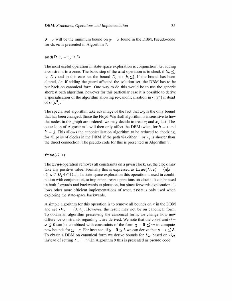
will be the minimum bound on found in the DBM. Pseudo-codefor down is presented in Algorithm 7.
and( )
The most useful operation in state-space exploration is conjunction, i.e. addinga constraint to a zone. The basic step of the and operation is to check if
and in this case set the bound to . If the bound has beenaltered, i.e. if adding the guard affected the solution set, the DBM has to beput back on canonical form. One way to do this would be to use the genericshortest path algorithm, however for this particular case it is possible to derivea specialisation of the algorithm allowing re-canonicalisation in insteadof .
The specialised algorithm take advantage of the fact that is the only boundthat has been changed. Since the Floyd-Warshall algorithm is insensitive to howthe nodes in the graph are ordered, we may decide to treat and last. Theouter loop of Algorithm 1 will then only affect the DBM twice, for and
. This allows the canonicalisation algorithm to be reduced to checking,for all pairs of clocks in the DBM, if the path via either or is shorter thanthe direct connection. The pseudo code for this is presented in Algorithm 8.
free( )
The free operation removes all constraints on a given clock, i.e. the clock maytake any positive value. Formally this is expressed as free
. In state-space exploration this operation is used in combi-nation with conjunction, to implement reset operations on clocks. It can be usedin both forwards and backwards exploration, but since forwards exploration al-lows other more efficient implementations of reset, free is only used whenexploring the state-space backwards.
A simple algorithm for this operation is to remove all bounds on in the DBMand set . However, the result may not be on canonical form.To obtain an algorithm preserving the canonical form, we change how newdifference constraints regarding are derived. We note that the constraint
can be combined with constraints of the form to computenew bounds for . For instance, if we can derive that .To obtain a DBM on canonical form we derive bounds for based oninstead of setting .In Algorithm 9 this is presented as pseudo code.

36 DBM: Structures, Operations and Implementation
reset( )
In forwards exploration this operation is used to set clocks to specific values,i.e. reset . Without the requirement thatoutput should be on canonical form, reset can be implemented by setting
, and remove all other bounds on . However,if we instead of removing the difference constraints compute new values usingconstraints on the other clocks, like in the implementation of free, we obtainan implementation that preserve the canonical form. Such an implementation ispresented in Algorithm 10.
copy( )
This is another operation used in forwards state-space exploration. It copiesthe value of one clock to another. Formally, we define reset as
. Analogous with reset, copy can be implementedby assigning , , removing all other bounds on andre-canonicalise the zone. However, a more efficient implementation is obtainedby assigning , and then copy the rest of the boundson from . For pseudo code, see Algorithm 11
shift( )
The last reset operation is shifting a clock, i.e. adding or subtracting a clock withan integer value, i.e. shift .The definition gives a hint on how to implement the operation. We can view theshift operation as a substitution of for in the zone. With this reasoning
is added to the upper and lower bounds of . However, since lower boundson are represented by constraints on , is subtracted from all thosebounds. This operation is presented in pseudo-code in Algorithm 12
3.3 Normalisation Operations
norm ( )
To obtain a finite zone graph most verifiers use some kind of normalisation ofzones. One of the key steps in most normalisation algorithms is the so called -normalisation, i.e. the zone is normalised with respect to the maximum constanteach clock is compared to in the automaton.

DBM: Structures, Operations and Implementation 37
The procedure to obtain the -normalisation of a given zone is to remove allbounds such that and to set all boundssuch that to . This corresponds to removing allupper bounds higher than the maximum constant and lowering all lower boundshigher than the maximum constant down to the maximum constant.
The -normalisation operation will not preserve the canonical form of the DBM,and in this case the best way to put the result back on canonical form is to useAlgorithm 1. Pseudo-code for -normalisation is given in Algorithm 13
reset( )
up( ) down( )
and( ) norm( ) shift
free( ) copy( )
Figure 5: All DBM operations applied to the same zone

38 DBM: Structures, Operations and Implementation
4 Zones in Memory
This section describes a number of techniques for storing zones in computermemory. The section starts by describing how to map DBM elements on ma-chine words. It continues by discussing how to place two-dimensional DBMsin one-dimensional memory and ends by describing how to store zones using asparse representation.
4.1 Storing DBM Elements
To store a DBM element in memory we need to keep track of the integer limitand whether it is strict or not. The range of the integer limit is typically muchlower than the maximum value of a machine word and the strictness can bestored using just one bit. Thus, it is possible to store both the limit and thestrictness in different parts of the same machine word. Since comparing andadding DBM elements are frequently used operations it is crucial for the per-formance of a DBM package that they can be efficiently implemented for thechosen encoding. Fortunately, it is possible to construct an encoding of boundsin machine words, where checking if is less than can be performed bychecking if the encoded is smaller than the encoded .
The encoding we propose is to use the least significant bit (LSB) of the ma-chine word to store whether the bound is strict or not. Since strict bounds aresmaller than non-strict we let a set (1) bit denote that the bound is non-strictwhile an unset (0) bit denote that the bound is strict. The rest of the bits in themachine word are used to store the integer bound. To encode we use thelargest positive number that fit in a machine word (denoted MAX_INT).
For good performance we also need an efficient implementation of addition ofbounds. For the proposed encoding Algorithm 4 adds two encoded boundsand . The symbols and in the algorithm are used to denote bitwise-andand bitwise-or, respectively.
Algorithm 4 Algorithm for adding encoded boundsif MAX_INT or MAX_INT then
return MAX_INTelse
returnend if

DBM: Structures, Operations and Implementation 39
4.2 Placing DBMs in Memory
Another implementation issue is how to store two-dimensional DBMs in linearmemory. In this section we present two different techniques and give a briefcomparison between them. The natural way to put matrices in linear memoryis to store the elements by row (or by column), i.e. each row of the matrix isstored consequently in memory. This layout has one big advantage, its goodperformance. This advantage is mainly due to the simple function for comput-ing the location of a given element in the matrix: .This function can (on most computers) be computed in only two instructions.This is important since all accesses to DBM elements use this function. Howthe different DBM elements are place in memory with this layout if presentedin Figure 6(a).
The second way to store a DBM in linear memory is based on a layered modelwhere each layer consists of the bounds between a clock and the clocks withlower index in the DBM. In this representation it is cheap to implement localclocks, since all information about the local clocks are localised at the end ofthe DBM. The drawback with this layout is the more complicated function fromDBM indices to memory locations. For this layout we have:
ifotherwise
This adds at least two instructions (one comparison and one conditional jump)to the transformation. This may not seem such a huge overhead, but it is clearlynoticeable. The cache performance is also worse when using this layout thanwhen storing the DBMs row-wise. This layout is illustrated in Figure 6(b).
The conclusion is that unless the tool under construction supports adding andremoving clocks dynamically the row-wise mapping should be used. On theother hand, if the tool supports local clocks the layered mapping may be prefer-able since no reordering of the DBM is needed when entering or leaving a clockscope.
4.3 Storing Sparse Zones
In most verification tools, the majority of the zones are kept in the set of statesalready visited during verification. They are used as a reference to ensure termi-nation by preventing states from being explored more than once. For the states

40 DBM: Structures, Operations and Implementation
(a) Row wise (b) Layered
Figure 6: Different layouts of DBMs in memory
in this set we may benefit from storing only the minimal number of constraintsusing a sparse representation.
A straight forward implementation is to store a sparse zone as a vector of con-straints of the form . We may save additional memory by omitting im-plicit constraints, such as . A downside with using sparse zones is thateach constraint require twice the amount of memory needed for a constraint ina full DBM, since the sparse representation must store clock indices explicitly.Thus, unless half of the constraints in a DBM are redundant we do not gainfrom using sparse zones.
A good feature of the sparse representation is that checking whether a zonerepresented as a full DBM is included in a sparse zone may be implementedwithout computing the full DBM for . It suffices to check for all constraintsin that the corresponding bound in is tighter. However, to check if
we have to compute the full DBM for .
5 Conclusions
In this paper we have reviewed Difference Bound Matrices as a data-structurefor timing constraints. We have presented the basics of the data-structure and alloperations needed in symbolic state-space exploration of timed automata. Wehave also discussed how to save space by computing the minimum number ofconstraints defining a given zone and saving them using a sparse representation.
References
[ABB 01] Tobias Amnell, Gerd Behrmann, Johan Bengtsson, Pedro R. D’Argenio,Alexandre David, Ansgar Fehnker, Thomas Hune, Bertrand Jeannet,Kim G. Larsen, M. Oliver Möller, Paul Pettersson, Carsten Weise, andWang Yi. UPPAAL - Now, Next, and Future. In Modelling and Verification

DBM: Structures, Operations and Implementation 41
of Parallel Processes, volume 2067 of Lecture Notes in Computer Science,pages 100–125. Springer-Verlag, 2001.
[AD90] Rajeev Alur and David L. Dill. Automata for modeling real-time systems.In Proceedings, Seventeenth International Colloquium on Automata, Lan-guages and Programming, volume 443 of Lecture Notes in Computer Sci-ence, pages 322–335. Springer-Verlag, 1990.
[AD94] Rajeev Alur and David L. Dill. A theory of timed automata. Journal ofTheoretical Computer Science, 126(2):183–235, 1994.
[BL96] Johan Bengtsson and Fredrik Larsson. UPPAAL a tool for automatic verifi-cation of real-time systems. Technical Report 96/67, Department of Com-puter Systems, Uppsala University, 1996.
[BY01] Johan Bentsson and Wang Yi. Reachability analysis of timed automatacontaining constraints on clock differences. Submitted for publication.,2001.
[Dil89] David L. Dill. Timing assumptions and verification of finite-state concur-rent systems. In Proceedings, Automatic Verification Methods for FiniteState Systems, volume 407 of Lecture Notes in Computer Science, pages197–212. Springer-Verlag, 1989.
[DOTY95] Conrado Daws, Alfredo Olivero, Stavros Tripakis, and Sergio Yovine. Thetool Kronos. In Proceedings, Hybrid Systems III: Verification and Con-trol, volume 1066 of Lecture Notes in Computer Science. Springer-Verlag,1995.
[Flo62] Robert W. Floyd. Acm algorithm 97: Shortest path. Communications ofthe ACM, 5(6):345, June 1962.
[Lar00] Fredrik Larsson. Efficient implementation of model-checkers for networksof timed automata. Licentiate Thesis 2000-003, Department of Informa-tion Technology, Uppsala University, 2000.
[LLPY97] Kim G. Larsen, Fredrik Larsson, Paul Pettersson, and Wang Yi. Effi-cient verification of real-time systems: Compact data structure and statespace reduction. In Proceedings, 18th IEEE Real-Time Systems Sympo-sium, pages 14–24. IEEE Computer Society Press, 1997.
[LPY97] Kim G. Larsen, Paul Petterson, and Wang Yi. UPPAAL in a nutshell. Jour-nal on Software Tools for Technology Transfer, 1997.
[Pet99] Paul Pettersson. Modelling and Verification of Real-Time Systems UsingTimed Automata: Theory and Practice. PhD thesis, Uppsala University,1999.
[Yov97] Sergio Yovine. Kronos: a verification tool for real-time systems. Journalon Software Tools for Technology Transfer, 1, October 1997.

42 DBM: Structures, Operations and Implementation
A Pseudo-CodeAlgorithm 5 relation( )
tttt
for to dofor to do
end forend forreturn
Algorithm 6 up( )
for to do
end for
Algorithm 7 down( )
for to do
for to doif then
end ifend for
end for

DBM: Structures, Operations and Implementation 43
Algorithm 8 and( )
if then
else if then
for to dofor to do
if then
end ifif then
end ifend for
end forend if
Algorithm 9 free( )
for to doif then
end ifend for
Algorithm 10 reset(
for to do
end for

44 DBM: Structures, Operations and Implementation
Algorithm 11 copy( )
for to doif then
end ifend for
Algorithm 12 shift( )
for to doif then
end ifend for
Algorithm 13 norm ( )
for to dofor to do
if and then
else if and then
end ifend for
end forclose( )

Paper B:Reachability Analysis of Timed Automata Containing Constraintson Clock Differences
Johan Bengtsson and Wang Yi.


Timed Automata with Constraints on Clock Differences 47
Reachability Analysis of Timed Automata ContainingConstraints on Clock Differences
Johan Bengtsson and Wang Yi
Department of Computer Systems, Uppsala University, Sweden.E-mail: {johanb,yi}@docs.uu.se
Abstract. The key step to guarantee termination of reachability analysisfor timed automata is the normalisation algorithms for clock constraints(i.e. symbolic states represented as DBM’s). It transforms DBM’s whichmay contain arbitrary constants into their equivalent according to max-imal constants appearing in clock constraints of an automaton. A re-striction of the existing algorithms is that clock constraints in timedautomata must be in the form [AD94] of where is a clock,
, and is a natural number. It was discovered re-cently that the existing tools were either providing incorrect answers ornot terminating when they are used to verify automata containing dif-ference constraints of the form: (that are indeed needed inmany applications e.g. in solving scheduling problems). In this paper, wepresent new normalisation algorithms that transforms DBM’s accordingto not only maximal constants of clocks but also difference constraintsappearing in an automata. To our knowledge, they are the first publishednormalisation algorithms for timed automata containing difference con-straints. The algorithms have been implemented in UPPAAL, demonstrat-ing that little extra overhead is needed to deal with difference constraints.
1 Introduction
Following the work of Alur and Dill on timed automata [AD94], a number ofmodel checkers have been developed for modelling and verification of timedsystems with timed automata as the core of their input languages [DOTY95,Yov97, LPY97, ABB 01] based on reachability analysis. The foundation fordecidability of reachability problems for timed automata is Alur and Dill’s re-gion technique, by which the infinite state space of a timed automaton due tothe density of time, may be partitioned into finitely many equivalence classesi.e. according to regions in such a way that states within each class will alwaysevolve to states within the same classes. However, analysis based on the re-gion technique is practically infeasible due to the large number of equivalence

48 Timed Automata with Constraints on Clock Differences
classes [LPY95], which is highly exponential in the number of clocks and theirmaximal constants.
One of the major advances in the area after the pioneering work of Alur and Dillis the symbolic technique [Dil89, YL93, HNSY94, YPD94, LPY95], whichtransforms the reachability problem to that of solving simple constraints. Itadopts the idea from symbolic model checking for untimed systems, which useslogical formulas to represent set of states and operations on formulas to repre-sent state transitions. It is proven that the infinite state-space of timed automatacan be finitely partitioned into symbolic states which are represented and ma-nipulated using a class of linear constraints known as zones and representedas Difference Bound Matrices (DBM) [Bel57, Dil89]. The reachability relationover symbolic states can be represented and computed by a few efficient oper-ations on zones. From now on, we shall not distinguish the terms: constraint,zone and DBM.
The technique can be simply formulated in an abstract reachability algorithm1
as shown in Algorithm 1. The algorithm is to check whether a timed automatonmay reach a final location . It explores the state space of the automaton interms of symbolic states in the form where is a location and is a zone(represented as a DBM).
Algorithm 1 Symbolic reachability analysisPASSED WAITwhile WAIT do
take from WAITif then return “YES”if for all PASSED then
add to PASSEDfor all such that do
add to WAITend for
end ifend whilereturn “NO”
Having a closer look at the algorithm, one will realize that termination is notguaranteed unless the number of constraints generated is finite or the constraints
1Several verification tools for timed systems (e.g. UPPAAL [BLL 96]) have been imple-mented based on this algorithm.

Timed Automata with Constraints on Clock Differences 49
form a well quasi-ordering with respects to set-inclusion (over solution sets forclock constraints) [Hig52]. There have been several normalisation algorithmsfor clock constraints represented as DBMs (e.g. [Rok93, Pet99]) that are thekey step to guarantee termination for the existing tools. They transform DBMswhich may contain arbitrary constants into their equivalent with maximal con-stants appearing in clock constraints. The transformation respects region equiv-alence and therefore the number of DBMs explored is finite. However a re-striction of the existing normalisation algorithms is that clock constraints in thesyntax of timed automata must be in the form [AD94] of where is aclock variable, is a relational operator and is a natural number. It was dis-covered recently that the existing tools were either providing incorrect answersor not terminating when they are used to verify automata containing differenceconstraints of the form: (that are indeed needed in many applicationse.g. in solving scheduling problems).
A normalisation algorithm based on region equivalence treats clock values abovea certain constant as equivalent. This is correct only when no guard of the form:
is allowed in an automaton. Otherwise the normalisation opera-tion may enlarge a zone so that the guard (a difference constraint) labelled on atransition is made true and thus incorrectly enables the transition. For automatacontaining difference constraints as guards, we need a finer partitioning, sincethe difference constraints introduce diagonal lines that split the entire clockspace, even above the maximum constants for clocks. The partitioning and re-lated normalisation operation based on region construction is too crude.
We demonstrate this by an example. Consider the example shown in Figure 1.The final location of the automaton is not reachable according to the semantics.This is because in location , the clock zone is ( and ) wherethe guard is ( and ) which is equivalent to ( and
and ) can never be true and thus disables the last transition.However, because the maximal constants for clock is (and for ), the zonein location : ( and ) will be normalised to ( and
) by the maximal constant for , which enables the guard ( and) leading to the final location. Thus the symbolic reachability analysis
based on a standard normalisation algorithm would incorrectly conclude thatthe last location is reachable.
In [BDGP98], it has been proved that a timed automaton with constraints onclock differences can be transformed to an equivalent automaton without con-straints on differences. However, this approach is impractical to be implementedin the existing tools that support debugging of models because the transfor-

50 Timed Automata with Constraints on Clock Differences
S0 S1 S2 S3
z:=0
y>2
y:=0x<z+1, z<y+1
Figure 1: Bug example
mation will change the syntax of the original automaton. In this paper, wepresent two normalisation algorithms that allow not only clock comparisonwith naturals but also comparison between clocks i.e. constraints on clock dif-ferences. The algorithms transform DBMs according to not only the maximalconstants of clocks but also difference constraints appearing in an automaton.To our knowledge, they are the first published normalisation algorithms fortimed automata containing difference constraints. The algorithms have beenimplemented in UPPAAL. Our experiments demonstrate that almost no extraoverhead is added to deal with difference constraints.
The paper is organised as follows: Section 2 reviews timed automata and reach-ability analysis. Section 3 introduces the problem in normalising symbolic statesfor timed automata with constraints over clock differences. Section 4 presentstwo new normalisation algorithms. Section 5 concludes the paper.
2 Preliminaries
In this section we briefly review the notation for timed automata and its seman-tics. More extensive descriptions can be found in e.g. [AD94, Yov98, Pet99].
2.1 Timed Automata Model
Let be a finite set of labels, ranged over by etc. A timed automaton is afinite state automaton over alphabet extended with a set of real valued clocks,to model time dependent behaviour. Let denote a set of clocks, ranged over by
, and define as the set of conjunctions of atomic constraints of theform and for and . We usefor the subset of where all atomic constraints are of the form andlet range over this set.

Timed Automata with Constraints on Clock Differences 51
Definition 1 (Timed Automaton) A timed automaton is a tuplewhere is a set of control nodes, is the initial node,
is the set of edges and assign invariants tolocations. As a simplification we will use to denote .
The clocks values are formally represented as functions, called clock assign-ments, mapping to the non-negative reals . We let denote such func-tions, and use to denote that the clock assignment satisfy the formula .For we use for the clock assignment that map all clocks in tothe value , and for we let denote the clock assignmentthat map all clocks, , in the domain of to and agree with for the otherclocks in
The semantics of a timed automaton is a timed transition-system where thestates are pairs , with two types of transitions, corresponding to delay tran-sitions and discrete action transitions respectively:
if and
if and
It is easy to see that the state space for such a transition system is infinite andthus not adequate for algorithmic verification. However, efficient algorithmsmay be obtained using a symbolic semantics based on symbolic states of theform , where [HNSY92, YPD94]. The symbolic counterpartof the transitions are given by:
if
where and . It can beshown that the set of constraint systems is closed under these operations, in thesense that the result of the operations can be expressed by elements of .
Moreover the symbolic semantics correspond closely to the standard semanticsin the sense that if then, for all there is suchthat .
2.2 Reachability Analysis
Given a timed automaton with symbolic initial-state and a symbolicstate , is said to be reachable if and

52 Timed Automata with Constraints on Clock Differences
for some . This problem may be solved using a standard reachability algo-rithm for graphs. However the unbounded clock values may render an infinitezone graph and thus might the reachability algorithm not terminate. The solu-tion to this problem is to obtain a finite symbolic semantics by normalising thestates with respect to the maximum constant each clock is compared to in theautomaton. For details we refer the reader to [Pet99, Rok93] but the main factand the intuition behind it is described here. In order to do this we first haveto introduce the notion of closed constraint systems. We say that a constraintsystem is closed under entailment or just closed, for short, if noconstraint in can be strengthened without reducing the solution set.
Proposition 1 For each constraint system there is a unique con-straint system such that and have exactly the same solutionset and is closed under entailment.
From this proposition we conclude that a closed constraint system can be usedas a canonical representation of a zone.
Given a zone and a set of maximal constants wheredenotes the maximal constant for clock , the normalisation of , denotednorm , is computed from the closed representation of by
1. Removing all constraints of the form , , andwhere ,
2. Replacing all constraints of the form , , andwhere with and respectively.
This can then be used to define a notion of normalised symbolic transitions( ) by modifying the transitions of the standard symbolic semantics to pre-serve normalisation. The discrete action transition already preserves this sothere is no need to modify it, but the delay transition should be modified to
norm .
Proposition 2 Assume a timed automaton with initial-state and letbe the set of maximal constants used to compare with respective clocks in. Then is reachable from if and only if there is a sequence of
normalised transitions such that .
Using this we get a finite symbolic state-space where we can apply a standardreachability algorithm for graphs, such as the one in Algorithm 1 with the sym-bolic transition relation being replaced with the normalised version .

Timed Automata with Constraints on Clock Differences 53
3 Constraints on Clock Differences and Normalisation
Timed automata can easily be extended to allow guards where the differencebetween two clocks is compared, i.e. allowing the guards to be taken from thefull set , not only from . However, this extension do not give moreexpressive power; it has been shown (e.g. in [BDGP98]) that a timed automatonwith difference constraints can be transformed into an equivalent automatonwithout difference constraints. From now on, we will call the timed automatadescribed in Section 2 for diagonal free timed automata and widen the termtimed automata to include also automata with difference constraints.
We note that for diagonal-free timed automata the normalisation algorithm de-scribed earlier is based on the so called region equivalence.
Definition 2 (Region Equivalence) For a clock , let be a constant(the ceiling of clock ). For a real number , let denote the fractional partof , and denote its integer part. Two clock assignments are region-equivalent, denoted , iff
1. for each clock , either or and ,and
2. for all clocks if and then
(a) iff and
(b) iff
For the extended version we need a finer partitioning, since the difference con-straints in the guards introduce diagonal lines that split the entire clock space,even above the maximum constants for the clocks. The partitioning used fordiagonal-free automata, and the connected normalisation operation norm istoo crude. We demonstrate this by an example: Consider the timed automatonin Figure 2. The automaton has two clocks, (with maximum constant 0) and
(with maximum constant 1). The only difference constraint in the example is. This will be used as a running example throughout the paper since the
small number of clocks make it possible to show the zones using graphs.
The problem is easily detected by comparing the clock zones of the unnor-malised symbolic semantics (presented in Figure 3) with the correspondingclock zones in the normalised symbolic semantics (presented in Figure 4). Tohighlight the cause of the problem even further we show borders between equiv-alence classes in the clock space ( from the maximum constant for and

54 Timed Automata with Constraints on Clock Differences
S0 S1 S2 S3x:=2 y<1 x-y<=0
Figure 2: Example automaton with difference guards
from the difference constraint) as dashed lines. The initial state of theautomaton is After performing the first action step it will reach thestate . Idling in location leads to the state .Since this is above the maximum constant of the corresponding state in thenormalised semantics will be . Thus, the normalised state will, er-roneously, contain time assignments from the triangle eventhough no state in the real semantics has a time assignment in this equiv-alence class. Performing the next action step will take the automaton to thestate . The next step in the normalised seman-tics is the state . The automaton may now idle to the state
. The corresponding state in the normalised se-mantics is . In the real semantics no further step is possiblesince the guard is not satisfied while the normalised semantics mayproceed to location since the time assignments satisfying arepresent in the normalised states. The conclusion is that the normalisation pro-cedure have to be adapted to handle timed automata with difference constraints.
4 New Normalisation Algorithms
In this section we will present how to normalise the symbolic states for a timedautomaton with difference constraints together with two slightly different algo-rithms to do this. The first algorithm is simpler, and may still yield an infinitezone graph. However, the zones form a well quasi-order with respect to inclu-sion checking and thus the reachability algorithm is guaranteed to terminate(see e.g. [ACJT00]). The second algorithm is more complex and does not suf-fer from this problem, but it may require splitting of symbolic states.

Timed Automata with Constraints on Clock Differences 55
Leaving S0 Entering S1 Leaving S1
Entering S2 Leaving S2 Entering S3
Figure 3: Zones for the example automaton, without normalisation
Leaving S0 Entering S1 Leaving S1
Entering S2 Leaving S2 Entering S3
Figure 4: Zones for the example automaton, with incorrect normalisation
56 Timed Automata with Constraints on Clock Differences
4.1 Region Equivalence Refined by Difference Constraints
The key issue for the extended normalisation algorithms is to honour the equiv-alence classes that are introduced by difference constraints in the guards. Wenote that difference constraints in the guards may introduce equivalence classesin the clock space that reach beyond any maximum constant. Thus we need torefine the region equivalence from Definition 2 to take the difference constraintsinto account.
Definition 3 (Refined Region Equivalence) Let be a finite set of constraintsof the form for , and . Two clockassignments are equivalent, iff and
We note that since the number of regions defined by is finite and there areonly finitely many constraints in this refined region equivalence will definefinitely many regions.
4.2 The Core of Normalisation
We can now use the refined region equivalence from Definition 3 to obtain thecore of a normalisation algorithm. From the region equivalence we get the needto ensure that if a difference constraint is not satisfied by any point in the unnor-malised zone, , then it should not be satisfied by any point in the normalisedzone, norm , and if all points in satisfy a difference constraint then soshould all points in norm . This leads to a core normalisation algorithmconsisting of three stages:
1. Collect all difference constraints from that are not satisfied by any pointin the zone and the negation of all difference constraints that are satisfiedby all points in the zone.
2. Perform normalisation with respect to the maximum constants of .
3. Apply the negation of all the collected constraints to the normalised zoneto make sure that none of the collected constraints are satisfied after nor-malisation.
In Algorithm 2 this core normalisation is given as pseudo code. The setreferred to in the algorithm is the set of difference constraints in and theoperation norm refers to normalisation with respect to the maximum constantsof .

Timed Automata with Constraints on Clock Differences 57
Algorithm 2 Core normalisation algorithm
for all such that or doif then
end ifend for
normfor all do
end forreturn
However, there are cases where this algorithm is incorrect with respect to theequivalence classes. For some cases when a difference constraint split the zoneto be normalised, the perfect normalisation may not be represented using a sin-gle zone. One instance of such a zone is the “leaving S1” zone in our runningexample. If this zone was extended to contain the set of equivalence classes,from which it contains points, it would be the whole clock space except for thesmall triangle defined by . The main difference between the twoproposed algorithms is how this is resolved.
4.3 Algorithm: Normalisation without Zone Splitting
The first normalisation algorithm is based on the observation that due to thegeometry of the equivalence classes, the problem will only occur when the zoneis stretched downwards, i.e. when the lower bound of the zone is lowered downto the maximum constant. Thus, if the zones are not stretched downwards whennormalising the problem can be avoided. This gives an algorithm that is similarto core normalisation presented in Algorithm 2, with the only exception thatthe step of replacing constraints of the form and
for is removed from the norm -operation.
The problem with this solution is that the normalised zone graph is no longerfinite, since delay may cause the lower bound of the zone to increase unbound-edly. However, the normalised zones are well quasi-ordered with respect to zoneinclusion and thus the termination of the reachability algorithm can be guaran-teed [ACJT00].

58 Timed Automata with Constraints on Clock Differences
Using this normalisation procedure for our example automaton will give thezones presented in Figure 5. We note from the figure that now the normalisedzones does not contain time assignments from equivalence classes not in thecorresponding unnormalised zone. Further we see that the zones are not ex-panded to fill all the equivalence classes where it has points.
4.4 Algorithm: Normalisation with Zone Splitting
The second normalisation procedure is based on the observation that the prob-lem only occurs when a difference constraint divides the unnormalised zone,i.e. some of the time assignments in the zone satisfy the difference constraintand some do not. Thus, if all such zones are split along dividing differenceconstraints, e.g. using Algorithm 3, before normalisation this problem can beavoided.
Algorithm 3 Zone splitting algorithm
for all dofor all do
if and then
else
end ifend for
end forreturn
The full normalisation procedure is presented in Algorithm 4. The splitting,denoted by split in the description, is used as a preprocessing step and then thebasic normalisation algorithm, norm , is applied to all the resulting zones. Weuse norm to denote this normalisation operation and we use this operation todefine a normalised symbolic transition relation.
Definition 4 Let be a timed automaton with the symbolic semantics .The -normalised version of ( ) for is defined by: whenever
then for all norm .
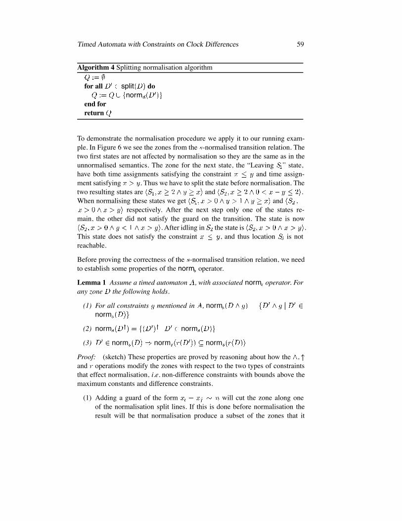
Timed Automata with Constraints on Clock Differences 59
Algorithm 4 Splitting normalisation algorithm
for all split donorm
end forreturn
To demonstrate the normalisation procedure we apply it to our running exam-ple. In Figure 6 we see the zones from the -normalised transition relation. Thetwo first states are not affected by normalisation so they are the same as in theunnormalised semantics. The zone for the next state, the “Leaving ” state,have both time assignments satisfying the constraint and time assign-ment satisfying . Thus we have to split the state before normalisation. Thetwo resulting states are and .When normalising these states we get and ,
respectively. After the next step only one of the states re-main, the other did not satisfy the guard on the transition. The state is now
. After idling in the state is .This state does not satisfy the constraint , and thus location is notreachable.
Before proving the correctness of the -normalised transition relation, we needto establish some properties of the norm operator.
Lemma 1 Assume a timed automaton , with associated norm operator. Forany zone the following holds.
(1) For all constraints mentioned in , normnorm
(2) norm norm
(3) norm norm norm
Proof: (sketch) These properties are proved by reasoning about how the ,and operations modify the zones with respect to the two types of constraintsthat effect normalisation, i.e. non-difference constraints with bounds above themaximum constants and difference constraints.
(1) Adding a guard of the form will cut the zone along oneof the normalisation split lines. If this is done before normalisation theresult will be that normalisation produce a subset of the zones that it
60 Timed Automata with Constraints on Clock Differences
would originally have produced. If the guard is added after normalisationa number of entire zones from the normalisation will be removed givingthe same final result.
Adding a guard of the form will cut away a part of the zone thatis not affected by the normalisation since, by definition,
(2) Difference constraints are not effected at all by the operation. Furtherdo not introduce any new non-difference constraints.
(3) operations are projections of a on a hyperplane defined by . Thisprojection has the property that points that were added by normalisationare mapped to other that would be added by renormalisation.
Finally we prove that the -normalised transition relation is correct.
Theorem 1 Let be a timed automaton and for each clock let bethe largest number is compared to in .
(Soundness) whenever thenfor all such that
(Completeness) whenever thenfor some such that
Proof: Both soundness and completeness are proven by induction on the lengthof the transition sequences.
(Soundness) As induction hypothesis, assumesuch that and norm . Further assume
. We now need to prove that such thatnorm , and norm . We havetwo cases: delay transitions and action transitions.
(Delay) By the assumption by delay, and thedefinition of we get norm . Combining thiswith Lemma 1 (1+2) gives normnorm , and since is already normalised we get
, i.e. . Now assume that for all suchthat norm and by delay,norm . By the definition of we have ,which gives norm norm . Expansion usingLemma 1 (1+2) yields norm

Timed Automata with Constraints on Clock Differences 61
norm . By our assumption, norm andnorm , for all , but this lead to a contradiction.
(Action) By assumption we know that by. From the definitions of norm and we can derive that
for all such that norm , byNow we need to prove that such that
norm . By the definition of , norm norm. Expansion by Lemma 1(1) gives normnorm . According to Lemma 1(1+3) and
norm we have norm norm .And since we know, by the definition of , that norm
we conclude that norm .
(Completeness) As induction hypothesis, assumesuch that and . Further assume
. We need to prove that such that ,and . There are two cases, or .
( ) By the assumption we know, i.e. . From the
definition of we have by delay, ifnorm . Expansion by the definition of yieldsnorm . By the definition of normwe know that for all zones , norm . Thus there is azone norm such that
( ) By the assumption we know, , . From the definition of we have
by if norm. Expanding this by the definition of the -operation yields
norm . By the def-inition of norm we know that for all zones , norm .Thus there is a zone norm such that
.

62 Timed Automata with Constraints on Clock Differences
Leaving S0 Entering S1 Leaving S1
Entering S2 Leaving S2 Entering S3
Figure 5: Zones for the example automaton, with non splitting normalisation.
1
2
Leaving S0 Entering S1 Leaving S1
Entering S2 Leaving S2 Entering S3
Figure 6: Zones for the example automaton, with splitting normalisation.

Timed Automata with Constraints on Clock Differences 63
5 Conclusion
In modelling and verifying timed systems, using timed automata, constraintsover clock differences are useful and needed in many applications e.g. solvingscheduling problems. In this paper, we have reported a problem in the existing(published) symbolic reachability algorithms for timed automata. The problemis that the existing normalisation algorithms (implemented by several verifica-tion tools for timed automata e.g. UPPAAL) for clock constraints based on re-gion equivalence are incorrect in the sense that they may provide wrong answersin verifying timed automata containing constraints on clock differences. Thereason is that the normalisation operations may enlarge a zone so that the guard(a difference constraint) labelled on a transition is made true and thus incor-rectly enables the transition. Thus the normalisation operation should be basedon a finer equivalence relation than region equivalence. We propose to use theregion equivalence which is further refined by difference constraints. Based onthis, we have developed two normalisation algorithms that allow not only clockcomparison with naturals but also comparison between clocks i.e. constraintson clock differences. The algorithms transform DBM’s according to not onlythe maximal constants of clocks but also difference constraints appearing inan automaton. To our knowledge, they are the first published normalisation al-gorithms for timed automata containing difference constraints. The algorithmshave been implemented in UPPAAL showing that almost no extra overhead isadded to deal with difference constraints.
References
[ABB 01] Tobias Amnell, Gerd Behrmann, Johan Bengtsson, Pedro R. D’Argenio,Alexandre David, Ansgar Fehnker, Thomas Hune, Bertrand Jeannet,Kim G. Larsen, M. Oliver Möller, Paul Pettersson, Carsten Weise, andWang Yi. UPPAAL - Now, Next, and Future. In Modelling and Verificationof Parallel Processes, number 2067 in Lecture Notes in Computer Science,pages 100–125. Springer-Verlag, 2001.
[ACJT00] Parosh Aziz Abdulla, Karlis Cerans, Bengt Johnsson, and Yih-Kuen Tsay.Algorithmic analysis of programs with well quasi-ordered domains. Jour-nal of Information and Computation, 160:109–127, 2000.
[AD94] Rajeev Alur and David L. Dill. A theory of timed automata. Journal ofTheoretical Computer Science, 126(2):183–235, 1994.

64 Timed Automata with Constraints on Clock Differences
[BDGP98] Beatrice Bérard, Volker Diekert, Paul Gastin, and Antoine Petit. Charac-terization of the expressive power of silent transitions in timed automata.Fundamenta Informaticae, 36:145–182, 1998.
[Bel57] Richard Bellman. Dynamic Programming. Princeton University Press,1957.
[BLL 96] Johan Bengtsson, Kim G. Larsen, Fredrik Larsson, Paul Pettersson, andWang Yi. UPPAAL in 1995. In Proc. of the 2nd Workshop on Tools andAlgorithms for the Construction and Analysis of Systems, number 1055in Lecture Notes in Computer Science, pages 431–434. Springer–Verlag,March 1996.
[Dil89] David L. Dill. Timing assumptions and verification of finite-state concur-rent systems. In Proceedings, Automatic Verification Methods for FiniteState Systems, volume 407 of Lecture Notes in Computer Science, pages197–212. Springer-Verlag, 1989.
[DOTY95] Conrado Daws, Alfredo Olivero, Stavros Tripakis, and Sergio Yovine. Thetool kronos. In Proceedings, Hybrid Systems III: Verification and Con-trol, volume 1066 of Lecture Notes in Computer Science. Springer-Verlag,1995.
[Hig52] Graham Higman. Ordering by divisibility in abstract algebras. Proceed-ings of the London Mathematical Society, Ser. 3, 2:326–336, 1952.
[HNSY92] Thomas A. Henzinger, Xavier Nicollin, Joseph Sifakis, and Sergio Yovine.Symbolic model checking for real-time systems. In Proceedings, SeventhAnnual IEEE Symposium on Logic in Computer Science, pages 394–406,1992.
[HNSY94] Thomas A. Henzinger, Xavier Nicollin, Joseph Sifakis, and Sergio Yovine.Symbolic model checking for real-time systems. Technical Report TR94-1404, Cornell Computer Science Technical Report Collection, 1994.
[LPY95] Kim G. Larsen, Paul Pettersson, and Wang Yi. Compositional and Sym-bolic Model-Checking of Real-Time Systems. In Proc. of the 16th IEEEReal-Time Systems Symposium, pages 76–87. IEEE Computer SocietyPress, December 1995.
[LPY97] Kim G. Larsen, Paul Petterson, and Wang Yi. Uppaal in a nutshell. Journalon Software Tools for Technology Transfer, 1997.
[Pet99] Paul Pettersson. Modelling and Verification of Real-Time Systems UsingTimed Automata: Theory and Practice. PhD thesis, Uppsala University,1999.
[Rok93] Tomas Gerhard Rokicki. Representing and Modeling Digital Circuits.PhD thesis, Stanford University, 1993.

Timed Automata with Constraints on Clock Differences 65
[YL93] Mihalis Yannakakis and David Lee. An efficient algorithm for minimiz-ing real-time transition systems. In Proceedings, Fifth International Con-ference on Computer Aided Verification, volume 697 of Lecture Notes inComputer Science, pages 210–224. Springer-Verlag, 1993.
[Yov97] Sergio Yovine. Kronos: A verification tool for real-time systems. Journalon Software Tools for Technology Transfer, 1, October 1997.
[Yov98] Sergio Yovine. Model checking timed automata. In European EducationalForum: School on Embedded Systems, volume 1494 of Lecture Notes inComputer Science, pages 114–152. Springer-Verlag, 1998.
[YPD94] Wang Yi, Paul Petterson, and Mats Daniels. Automatic verification of real-time communicating systems by constraint-solving. In Proceedings, Sev-enth International Conference on Formal Description Techniques, pages223–238, 1994.


Paper C:Reducing Memory Usage in Symbolic State-Space Exploration forTimed Systems
Johan Bengtsson and Wang Yi.


Reducing Memory Usage 69
Reducing Memory Usage in Symbolic State-SpaceExploration for Timed Systems
Johan Bengtsson and Wang Yi
Department of Computer Systems, Uppsala University, Sweden.Email: {johanb,yi}@docs.uu.se
Abstract. One of the major problems in scaling up model checkingtechniques to the size of industrial systems is memory consumption.This paper studies the problem in the context of verifiers for timed au-tomata. We present a number of techniques that reduce the amount ofmemory used in symbolic reachability analysis. We address the memoryconsumption problem on two fronts. First, we reduce the size of internalrepresentations for each symbolic state (clock constraints) by means ofcompression methods. Second, we reduce the explored state space (listof symbolic states) by early-inclusion checking between states and byprobabilistic methods. These techniques have been implemented in theUPPAAL tool. Their strengths and weaknesses are evaluated and com-pared in experiments using real-life examples. Note that though thesetechniques are developed for timed systems, they are of general interestsfor verification tool development, in particular to handle large symbolicstates based on constraint representation and manipulation.
1 Introduction
During the last ten years timed automata [AD90, AD94] have evolved as acommon model to describe timed systems. This process has gone hand in handwith the development of verification tools for timed automata, such as KRO-NOS [DOTY95, Yov97] and UPPAAL [LPY97, ABB 01]. One of the majorproblems in applying these tools to industrial-size systems is the large memoryconsumption (e.g. [BGK 96]) when exploring the state space of a network oftimed automata. The reason is that the exploration not only suffers from thelarge number of states to be explored, but also from the large size of each state.In this paper we address both these problems.
We will present techniques to reduce memory usage for internal representa-tions of symbolic states by means of compaction. We use two different meth-ods for packing states. First, we code the entire state as one large number us-
70 Reducing Memory Usage
ing a multiply-and-add algorithm. This method yields a representation that iscanonical and minimal in terms of memory usage but the performance for in-clusion checking between states is poor. The second method is mainly intendedto be used for the timing part of the state and it is based on concatenation ofbit strings. Using a special concatenation of the bit string representation of theconstraints in a zone, ideas from [PS80] can be used to implement fast inclusionchecking between packed zones.
Furthermore, we attack the problem with large state spaces in two differentways. First, to get rid of states that do not need to be explored, as early as pos-sible, we introduce inclusion checking already in the data structure holding thestates waiting to be explored. We also describe how this can be implementedwithout slowing down the verification process. Second, we investigate how su-pertrace [Hol91] and hash compaction [WL93, SD95] methods can be appliedto timed systems. We also present a variant of the hash compaction method, thatallows termination of branches in the search tree based on probable inclusionchecking between states.
The rest of the paper is organised as follows: In section 2 we introduce timedautomata and describe briefly how to check reachability properties for timedautomata. In section 3 we present methods to represent the key objects used inchecking timed automata, namely the symbolic states. We also give a compar-ison between them. Section 4 addresses issues on the whole state space of anautomaton. We describe how the wait and past lists are handled efficiently. Wealso describe an approximation method of the past list that can be used whenthe complete state space of an automaton is too big to be stored in memory. Fi-nally, section 5 wraps up the paper by summarising the most important resultsand suggests some directions for future work.
2 Preliminaries
In this section we briefly review background materials including timed au-tomata and reachability analysis based on clock constraints. A more extensivedescription can be found in e.g. [AD94, Pet99].
Let be a finite set of labels, ranged over by etc.A timed automaton is afinite state automaton over alphabet extended with a set of real valued clocks,to model time dependent behaviour. Let denote a set of clocks, ranged overby . Let denote the set of conjunctions of atomic constraints of the

Reducing Memory Usage 71
form or for and . Weuse and later to range over this set.
Definition 5 (Timed Automaton) A timed automaton is a tuplewhere is a set of control nodes, is the initial node,
is the set of edges and assign invariants tolocations. As a convention we will use to denote .
The clock values are formally represented as functions, called clock assign-ments, mapping to the non-negative reals . We let denote such func-tions, and use to denote that the clock assignment satisfy the formula
. For we let denote the clock assignment that map all clocksin to the value , and for we let denote the clock
assignment that map all clocks in to 0 and agree with for all clocks in .
The semantics of a timed automaton is a timed transition-system where thestates are pairs , with two types of transitions, corresponding to delay tran-sitions and discrete action transitions respectively:
if and
if and
It is easy to see that the state space is infinite and thus not a good base foralgorithmic verification. However, efficient algorithms may be obtained usinga symbolic semantics based on symbolic states of the form [HNSY92,YPD94] where is the location vector of an automaton and is a clockconstraint (zone) specifying the clock values. They are symbolic in the sensethat the clock zone represents a set of concrete states of the automaton with thesame control location vector. The symbolic counterpart of the transitions aregiven by:
if
where and . Itcan be shown that the set of constraint systems is closed under these operations.Moreover the symbolic semantics correspond closely to the standard semanticsin the sense that if then, for all there is suchthat .
Given a timed automaton with an initial symbolic state and a final sym-bolic state , is said to be reachable if

72 Reducing Memory Usage
and for some . The reachability problem can be solved usinga standard reachability algorithm as shown in Algorithm 1 for graphs with aproper normalisation algorithm for clock constraints [Pet99, Rok93] (to guar-antee termination).
The algorithm uses two important data structures: WAIT and PASSED. WAIT isa list of states waiting to be explored and PASSED is the set of states alreadyexplored. Due to the size of the state space, these structures may consume aconsiderable amount of main memory. The main objective of this paper is topresent techniques to reduce the memory usage of these two structures.
Algorithm 1 Symbolic reachability analysisPASSED WAITwhile WAIT do
take from WAITif then return “YES”if for all PASSED then
add to PASSEDfor all such that do
add to WAITend for
end ifend whilereturn “NO”
The core of the above reachability algorithm is manipulation and representationof symbolic states. So symbolic states are the core objects of state space search,and one of the key issues in implementing an efficient model checker is how torepresent them. The desired properties of the representation also differ in partsof the verifier, and there are potential gains in using different representations indifferent places.
The encoding of the location vector and the integer assignment is straight for-ward. For the location vector we number the locations in each process, to geta vector of location numbers. Representing the clock zone is a bit trickier butstarting from the constraint system representation of a zone it is possible toobtain an efficient intermediate representation. We start with the following ob-servation: Let be a dummy clock with the constant value 0. Then for eachconstraint system there is a constraint system withthe same solution set as , and where all constraints are of the formor , for .

Reducing Memory Usage 73
We also note that to represent any clock zone we need at mostatomic constraints. One of the most compact ways to represent this is to usea matrix where each element represent a bound on the difference between twoclocks. Each element in the matrix is a pair where is an integer and
tells whether the bound is strict or not. Such a matrix is called a DifferenceBounds Matrix, or DBM for short. More detailed information about DBMs canbe found in [Dil89].
3 Representing Symbolic States
Recall that symbolic states are pairs in the form where is the locationvector of an automaton represented as a vector of integers and is a clockconstraint (zone), represented as a matrix of integers (DBM). Logically such astate is a vector of integers representing the control locations and clock bounds.In the following, we study how to represent the vectors physically in the mainmemory for efficient storage and manipulation.
3.1 Normal Representation
The simplest way to physically represent a symbolic state is to use a machineword for each control location, integer value or clock bound. The implementa-tion is straight forward, but a practical tip is that if the standard library functionsfor memory management are used all the memory needed for one state should,if possible, be allocated in the same chunk, to minimise the allocation overhead.
The strength of this representation is its simplicity and the speed of accessing anindividual control location, integer value, or clock bound. In this representationthe maximum time needed to reach any individual entity is the time neededto fetch a word from the memory. This makes the representation ideal to usewhen we have to do operations on individual entities, e.g. when calculating thesuccessors of a state. The weakness is the amount of wasted space. Here a wholemachine word, typically 32-bit wide, is used to store entities where all possiblevalues may fit in many fewer bits.
However this is a good base representation for states. It is ideal for states thatwill be modified in the near future, such as intermediate states or states in WAIT.It also works reasonably well for states in PASSED, specially for small andmedium sized examples.
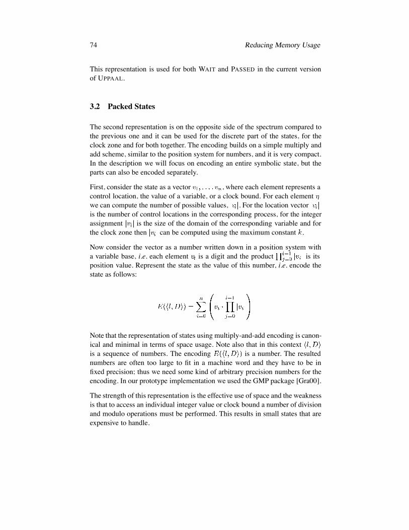
74 Reducing Memory Usage
This representation is used for both WAIT and PASSED in the current versionof UPPAAL.
3.2 Packed States
The second representation is on the opposite side of the spectrum compared tothe previous one and it can be used for the discrete part of the states, for theclock zone and for both together. The encoding builds on a simple multiply andadd scheme, similar to the position system for numbers, and it is very compact.In the description we will focus on encoding an entire symbolic state, but theparts can also be encoded separately.
First, consider the state as a vector , where each element represents acontrol location, the value of a variable, or a clock bound. For each elementwe can compute the number of possible values, . For the location vectoris the number of control locations in the corresponding process, for the integerassignment is the size of the domain of the corresponding variable and forthe clock zone then can be computed using the maximum constant .
Now consider the vector as a number written down in a position system witha variable base, i.e. each element is a digit and the product is itsposition value. Represent the state as the value of this number, i.e. encode thestate as follows:
Note that the representation of states using multiply-and-add encoding is canon-ical and minimal in terms of space usage. Note also that in this contextis a sequence of numbers. The encoding is a number. The resultednumbers are often too large to fit in a machine word and they have to be infixed precision; thus we need some kind of arbitrary precision numbers for theencoding. In our prototype implementation we used the GMP package [Gra00].
The strength of this representation is the effective use of space and the weaknessis that to access an individual integer value or clock bound a number of divisionand modulo operations must be performed. This results in small states that areexpensive to handle.

Reducing Memory Usage 75
Example Time Spacereal (Sec) relative real (MB) relative
Field Bus (Faulty 1)Field Bus (Faulty 2)Field Bus (Faulty 3)Field Bus (Fixed)B&ODACAPO (big)DACAPO (small)Fischer 5Fischer 6
Table 1: Performance for packed states with expensive inclusion checking
In order to test the performance of this representation, it is implemented in thePASSED structure in UPPAAL. The implementation is straight forward, howeverexpensive division and modulo operations have to be used, in order to comparethe DBMs bound by bound.
The result of the experiment is presented in Table 1 (as absolute figures andin relation to the current PASSED implementation in UPPAAL). We note thatwith this representation the space performance is very good, with reductionsof up to 70% compared to the current PASSED implementation. However thetime performance is poor, for one instance of Fischers protocol we notice aslowdown of almost 13 times and for one instance of the Field Bus protocol theslowdown is 8 times. The conclusion is that this representation should only beused in cases where main memory is a severe restriction.
3.3 Packed Zones with Cheap Inclusion Check
The main drawback of representing states using the number encoding given insection 3.2 is expensive inclusion checking. In this section we present a com-pact way of representing zones overcoming this drawback. The heart of thisrepresentation builds on an observation due to [PS80] that one subtraction canbe used to perform multiple comparisons in parallel.
Let denote the minimum number of bits needed to store all possible valuesfor one clock bound. The DBM is then encoded as a long bit string, where eachbound is assigned a bit wide slot. The value of the clock bound is put in

76 Reducing Memory Usage
the least significant bits in the slot and the extra, most significant bit, is usedas a test bit.
Since a zone is included in another zone if and only if each bound in theDBM representing is as tight as the same bound in the DBM representationof , inclusion checking is to check if all elements in one vector is less than orequal to the same bound in another vector. Using the new bit-string encodingof zones this can be checked using only simple operations like bitwise-and ( ),bitwise-or ( ), subtraction and test for equality.
Given two packed zones and , to check if first set all thetest bits in to zero and all the test bits in to one. In an implemen-tation the test bits are usually zero in the stored states and setting them to one isdone using a prefabricated mask . The test is then performed by calculating
. The result is read out of the test bits. If a test bit is one thecorresponding bound in is at least as tight as in and if a test bit is zero thecorresponding bound is tighter in than in . Thus, if all test bits are one wecan conclude that and if all the test bits are zero . It is worthnoting that “all test bits are one” is both necessary and sufficient to conclude
while “all test bits are zero” is only sufficient to conclude .
In an implementation of this scheme the main issue is how to handle the bitstrings. The easiest way is to let a bignum package handle everything. However,this may give a considerable overhead, specially in connection with memoryallocation, since the bignum packages are often tailored towards other types ofapplications. In UPPAAL we share the memory layout of the bignum packages,but to reduce the overhead we have implemented our own operations on top ofit.
In the physical representation, i.e. how the bit-string is stored in memory, thebit-string is chopped up into machine-word sized chunks, or limbs. The limbsare then packed in big-endian order, i.e. the least significant limb first, in anarray. If the bit string doesn’t fill an even number of machine words the lastlimb is padded with zero bits.
Noting that the effect of all operations needed for the inclusion check, exceptsubtraction, is local within the limb and that subtraction only passes one borrowbit to the next more significant limb, we can implement the inclusion check inone pass through the array of limbs instead of one pass for each operation. Theone pass inclusion check is shown in Algorithm 2. In the description we use
to denote the limb with index in and to denote a binarysubtraction of machine word size.

Reducing Memory Usage 77
Algorithm 2 Inclusion check for packed zones
for to limbs docmpif cmp then return “false”if then
else
end ifend forreturn “true”
Example Time Spacereal (Sec) relative real (MB) relative
Field Bus (Faulty 1)Field Bus (Faulty 2)Field Bus (Faulty 3)Field Bus (Fixed)B&ODACAPO (big)DACAPO (small)Fischer 5Fischer 6
Table 2: Performance for packed states with cheap zone coding
To evaluate the performance of this technique, it was implemented in the PASSEDstructure in UPPAAL. In the experiment the discrete part of each state is storedin PASSED using the compact representation from the previous section and thezone is stored using this technique. The results are presented in Table 2, both asabsolute figures and compared to the standard state representation. We note thatusing this method the space usage is typically reduced by about 40%, withoutincreased verification time. The verification time is actually reduced a little us-ing this scheme, even though the number of operations is increased. The reasonfor this is most certainly that the number of memory operations are reduced bythe smaller memory footprint of the states1.
1Memory operations are expensive compared to arithmetic operations, specially since thereis no temporal locality in verifiers.

78 Reducing Memory Usage
4 Representing the Symbolic State-Space
The two key data structures in a model checker are, as mentioned before, WAIT,that keeps track of states not yet explored, and PASSED, that keeps track ofstates already visited. Both these data structures tend to be large, and how torepresent them is an important issue for performance. In this section we de-scribe how to implement WAIT and how to improve its performance by addinginclusion checking. We also describe a standard implementation of PASSED aswell as an implementation where space is saved at the price of possibly incon-clusive answers.
4.1 Representing WAIT
In its most simple form WAIT is implemented as a linked list. This is easy toimplement and it is easy to control the search order by adding unexplored statesat the end, for breadth first search, or adding states at the beginning, for depthfirst search.
An optimisation in terms of both time and space is to check whether a statealready occur in WAIT before adding it. For a verifier based on explicit statesthis will only give minor improvements, mainly by keeping down the lengthof WAIT, but for a verifier based on symbolic states this may actually preventrevisiting parts of the state space.
We know, e.g. from [Pet99], that if then all states reachablefrom are also reachable from and thus we only have to explore
. So before adding a new state to WAIT we check all states alreadyin WAIT. If we find any state including we stop searching and throwaway since all states reachable from it are also reachable from a statealready scheduled for exploration. If no such state is found we add toWAIT. During the search through WAIT we also delete all states included in
in order to prevent revisiting parts of the state space.
There are some implementation issues that need consideration. The main issueis how to find all states in WAIT with same discrete part. The simplest way to dothis is to do a linear search through WAIT every time a state is added. However,using this solution it will be expensive to add states, even for examples whereWAIT is short. One solution to this is to implement WAIT using a structurewhere searching is cheap, e.g. a hash table. The problem with this solution isthat picking up states from WAIT will be expensive, at least for search strategies

Reducing Memory Usage 79
For search order
For inclusion check
Figure 1: Structure of WAIT
Example Time (Sec) Space (MB)no opt inclusion gain(%) no opt inclusion gain(%)
Field Bus (Faulty 1)Field Bus (Faulty 2)Field Bus (Faulty 3)Field Bus (Fixed)B&ODACAPO (big)DACAPO (small)Fischer 5Fischer 6
Table 3: Performance impact of inclusion check on WAIT
like breadth first and depth first, where the exploration order depends on theorder in which the states were added WAIT.
In the implemented solution, each state in WAIT is indexed using both a listand a hash table. The list part is used to keep the depth or breadth first orderingof states and to make it cheap to pick up states to explore. The hash table partis used to index the states in WAIT based on their location vector, in order tospeed up inclusion checking. A picture of this structure is shown in Figure 1.
To test the performance of this solution we compared the space and time neededto explore the state space of nine examples, for one version of UPPAAL with-out inclusion checking on WAIT and one version with the combined scheme.The result is shown in Table 3. It is worth noting that the version with inclu-sion checking is both significantly faster and less memory consuming than theversion without inclusion checking, for all examples except Fischers protocolwhich is, as mentioned in the appendix, not typical.

80 Reducing Memory Usage
4.2 Representing PASSED
The key feature needed by a representation of PASSED is that searching shouldbe cheap. For a symbolic verifier it is also crucial, at least performance wise,that finding states which includes a given state is possible and cheap. In UP-PAAL the standard PASSED is implemented as a hash table, where the key iscomputed from the discrete part of the state and collisions are handled by chain-ing. The reason for basing the hash key only on the discrete part is to simplifychecking for inclusion between states by making all related states end up in thesame hash bucket. It is easy to see that hashing only on the discrete part is asgood as we can do if we want this property. The reason for using chaining in-stead of open addressing to resolve conflicts is, apart from keeping related statestogether, mainly simplicity and eliminating the need for expensive rehashing.Judging by performance the choice could go either way, at least if rehashing isnot taken into account. More about this can be read in [Lar00].
For some models the memory needed for exact verification may exceed theamount of memory installed in the system where the verification takes place.This often occurs within the modelling phase before most bugs are removedfrom the model. During this phase the verification engine is often used as a toolto find the cause of unwanted behaviour and not primarily to prove the absenceof such behaviour. Under these premises it is desirable to use a method that canhandle larger systems but sometimes miss unwanted behaviour. Here we willdescribe two such methods. The first method is an application of the supertracealgorithm from [Hol91] on networks of timed automata. The second method isbased on the hash compaction method from [WL93, SD95].
4.3 Supertrace PASSED for Timed Automata
The main idea behind supertrace PASSED is from the following observation:The purpose of PASSED is only to keep track of whether a state have beenvisited or not, i.e. for each state we only need one bit of information. Thus,PASSED for a system of states can be implemented as an -bit wide bit vector.However, if is sufficiently large, even such a compact representation will betoo large to fit the memory of the system running the verifier. A way to tacklethis problem is to loosen the demand that the verification should be exact andallow false hits to be indicated, i.e. a previously unvisited state may, with someprobability, be reported as already visited. Such a false hit will be called anomission, as it causes a part of the state space to be omitted from the state space

Reducing Memory Usage 81
search. This affects the reachability search such that if a state is reported to benot reachable we can not conclude that it can not be reached since it might havebeen excluded by an omission.
The natural way to implement such a PASSED structure is to allocate a bit-vector of size , where , and hash each state to a value in .In the UPPAAL implementation of the supertrace algorithm the hash function issimilar to the first packing technique described in Section 3:
Note that a variation of this hash function (applied only to the location vectorand the integer assignment) is used in both the normal PASSED implementationand the cross-reference table of the WAIT list. It is also possible to enhancethe supertrace algorithm by implementing a way to change the hash functionbetween runs, in order to lower the probability that a part of the state spaceis omitted. A simple way to do this is to implement a generator of universalhash functions [CW79] and provide the user with a way to choose among thefunctions in the class.
The main drawback of the supertrace algorithm, when applied to timed au-tomata, is that inclusion between time zones can not be detected. The effect ofthis is that the number of explored states increases. This leads to longer veri-fication times and more states to enter in PASSED, with an increased omissionprobability as result.
To investigate the performance of this algorithm we have implemented it inUPPAAL. In the experiment we test the supertrace PASSED structure for threedifferent sizes: 16MB, 32MB and 64MB and compare it to the standard PASSEDimplementation of UPPAAL, to estimate the impact of collisions. The results ofthe experiment are presented in Table 4. For each of the examples the tableshows the collision frequency and an estimation on the fraction of the statespace not covered due to collisions.
In the table there are several interesting observations. First, for the Philips ex-ample the coverage is totally independent of the size of the PASSED structure.We get exactly the same collision frequency and coverage for all three runs.This is an indication that the hash function is far from optimal on this example.

82 Reducing Memory Usage
Example 16MB 32MB 64MBcollision omitted collision omitted collision omitted
Philips (Correct)B&ODACAPO (big)DACAPO (small)Fischer 5Fischer 6
Table 4: Frequency of collisions and the fraction of state space not covered (in) for three instances of the supertrace PASSED structure
Example Supertrace Classic16MB 32MB 64MB
Philips (Correct)Philips (Erroneous)B&ODACAPO (big)DACAPO (small)Fischer 5Fischer 6
Table 5: Time (in seconds) to explore the entire state space for three differentsupertrace PASSED lists for the standard PASSED list
We also note, when studying the big DACAPO example, that even though thecollision frequency is decreased the fraction of the state space not covered inthe search may increase. The reason for this may be that the collisions occur fordifferent states in the different runs and that the number of children for thesestates differ. (If a state with many children is omitted the coverage will be lessthan if a state with few children is omitted.)
To see how the supertrace algorithm behave time-wise we made an experi-ment where the verification time was measured and compared to the standardPASSED implementation in UPPAAL. The setting of this experiment is a littledifferent from the previous one. For this example we used inclusion checkingon WAIT, to speed up verification. This is the most likely setting when usingthe tool in practice. The result of this experiment is presented in Table 5. As wesee in the table the times for the supertrace is in the same order of magnitude asthe standard PASSED implementation.

Reducing Memory Usage 83
4.4 Hash Compaction for Timed Automata
Hash compaction evolved from the supertrace ideas as a way to lower the proba-bility of omissions in the verification process. It was first investigated in [WL93]and then further developed in [SD95].
The key observation for hash compaction is that the supertrace PASSED listcan be seen as representation of a set of hash values, where a set bit (1) in thetable represents that this hash value is in the set; while an unset bit (0) in thetable represent that it is not. Under the assumption that the set is sparse, i.e. thenumber of elements in the set is small compared to the number of elements notin it, a table of the elements might be a more compact representation of the set.With this solution the number of possible hash values is no longer bounded bythe number of bits in the main memory.
In the work presented in [WL93] a normal hash table is used to store the el-ements and the key into this table is computed from the elements themselves.In [SD95] the technique is developed further. As a way to decrease the proba-bility of false collisions the key into the table is computed from the state itself,instead of from the hash signature, using a different hash function. Since thehash signature and its entry in the table are computed using different hash func-tions two states have to collide in both the hash functions for a false collision tooccur.
There is an alternative way to view this second variation of hash compaction.Start with the supertrace PASSED list. To lower the probability of classifyingan unvisited state as already visited we increase the number of bits in eachentry of the hash table. (Given a fixed amount of memory this is done at theexpense of the number of entries in the table.) To separate different states thatend up at the same position in table we build a signature, e.g. a checksum,of the states and store this. To compute the checksum we choose a functionwith a low probability that two different states have the same signature, i.e.
should be as small as pos-sible. For this we use a hash function. If we take this one step further the combi-nation of the signature and the index into the hash table can be seen as differentparts of the same hash value. Some bits of this value are used to index into thehash table and some bits are stored in the table. A sketch of this is shown inFigure 2.
Given a fixed amount of memory there is a tradeoff where to put the borderbetween the index part and the signature part. For each bit we take away from

84 Reducing Memory Usage
index signature
Figure 2: The table index and the signature as one hash value.
the index part we may double the number of bits in the signature, but at theprice of less entries in PASSED.
So far we have not mentioned how to handle collisions within the hash table.Since there are now several possible values for the entries in the hash table, it ispossible to get collisions in the hash table. Since the main priority of this solu-tion is space, collisions are resolved using open addressing instead of chaining.This will save one pointer for each state entered into PASSED, and since thesignatures are, more or less, as big as a pointer we may fit twice as many statesin the same amount of memory with open addressing than with chaining. Theprice we pay for this choice is that the hash table might get full. Normallythis would only lead to an expensive rehashing but in our case the informationneeded to rehash an entry in the hash table is no longer available. This leavesus with two choices, we can either stop the verification and say that PASSEDis full and advice the user to try with a larger PASSED, or we can just skipadding the state to PASSED and hope that the search will terminate anyway. Inthe prototype implementation we have chosen the first alternative.
To evaluate hash compaction for timed automata, we used two slightly differentPASSED implementations. The difference between them lies in what we storein the hash table. In the first implementation we store signatures of entire sym-bolic states. This solution gives a very compact representation of each state inPASSED, but it has the drawback that inclusion between states in PASSED cannot be detected. This leads to potentially larger state spaces resulting in a higherpressure on the PASSED structure.
In the second PASSED implementation we try to get around this problem byseparating the discrete part and the clock zone. In this implementation we ap-ply the hash function only to the discrete part of the state. The clock zone iscompressed using the method from Section 3.3 and stored in the hash table to-gether with the signature. With this solution we aim at minimising the numberof states stored in PASSED. However, storing the full zone has a big drawback.The entries in PASSED are much bigger than for the other type. For a fixed
Reducing Memory Usage 85
memory-size this will give less entries in PASSED. A way around this would beto compress the zones further using a method that, with some probability, mightreport false inclusions. However, this has not been investigated in this paper.
As an introductory experiment all the examples are run with 47-bit signatures2for three different sizes of the hash table (16MB, 32MB and 64MB), and anestimate of the covered part of the state space is computed. In order to preventinterference from the inclusion check on WAIT, this feature is turned off. In thisexperiment we experienced no omissions, but for some examples the verifica-tion procedure did not terminate correctly.
The faulty Philips example can not be handled at all by PASSED implementationbased only on signatures; while it can be handled by the combined scheme whenthe size of the passed list is at least 32MB. The reason is that large parts of thestate space of this example is revisited since the first PASSED implementationonly can detect equal states and not inclusion between states. In contrast to thisexample, the large instance of the DACAPO example terminates for all sizesusing the first PASSED implementation, while it fails to do so for 16MB and32MB using the second. This is because, for each state, the zone informationis an order of magnitude larger than the size of the hash signature. This, incombination with the fact that (for this example) the number of explored statesare almost the same in both variations, lead to that 16MB is large enough whenusing signatures only while 64MB is needed for the combined scheme.
To study what the impact of the signature length on the fraction of the statespace that is omitted from exploration we perform an experiment with 7-bitsignatures.3 The result of this experiment can be seen in Table 6. As we see inthe table there are still problem instances where no omissions occur. We alsonote that where omissions occur, in all cases except one, less than one per milleof the state space is omitted from exploration.
As a final experiment we measure the run time and memory use for state spaceexploration with a PASSED structure based on hash compaction with 47-bit sig-natures and compare it to the run time for state space exploration using theclassic PASSED implementation in UPPAAL. To get as close as possible to anormal use situation, inclusion checking for WAIT is enabled in this experi-ment. The measured run times are listed in Table 7. We note from the table thatthe combined scheme (signatures of the discrete part + packed zone) is some-
2The size of the signature may seem a little odd, but in the implementation one bit is sacrificedto ensure that no used slot in the hash table can be mistaken for an empty.
3This is the smallest possible signature size in the current implementation.

86 Reducing Memory Usage
what faster, for all examples, than using only signatures. The reason for thisis the smaller number of states that is visited using the combined scheme. Wealso note that using hash compaction is somewhat slower than using the clas-sic PASSED implementation (for all examples except Fischers protocol). This ispartly due to the extra work needed to compute the signatures and partly due tothat the hash compaction implementation within UPPAAL is a prototype.
The measured memory use for the different examples is listed in Table 8. Fromthis table we note that for the large examples, i.e. Field Bus, the large DACAPOinstance and Fischer 6, there are significant reductions in memory usage. Wealso note that for some of the smaller examples the classic PASSED implemen-tation use less memory than the hash compaction. This suggests that the chosensize of the hash compaction is too large, and that these examples can be verifiedusing much smaller PASSED. A further observation is that the measured num-bers for hash compaction are larger than the requested size for PASSED. Thereason for this is that the listed values are the total memory used in the verifi-cation, i.e. the numbers also include WAIT, temporary storage and the binarycode. In a real application, this should be taken into account when deciding howmuch memory to reserve for PASSED.
5 Conclusions
This paper describes and evaluates three different ways to physically representsymbolic states in PASSED, in implementing verifiers for timed automata. Theevaluation shows that if space consumption is a main issue rather than timeconsumption then the multiply-and-add scheme can be used. For the evaluatedexamples this optimisation reduces the memory usage by up to 70% comparedto the current representation used in UPPAAL, at the price of 3–13 times slow-down due to expensive inclusion checking between states. In all other cases thestate should be represented using a mixed representation where the discrete partis represented using the multiply-and-add scheme and the zone is representedby concatenated bit strings separated by test bits. This packing scheme reducesthe memory usage with 35%–65% compared to the current version of UPPAAL.In most cases this representation also gives a minor speedup (1%–3%) com-pared to the current UPPAAL implementation.
Further the paper describes how to improve performance by checking for al-ready visited states not only on PASSED, but also on WAIT. For the evaluated

Reducing Memory Usage 87
Example signature signature+pack16MB 32MB 64MB 16MB 32MB 64MB
Philips (correct)Philips (faulty)B&ODACAPO (big)DACAPO (small)Fischer 5Fischer 6
Table 6: Fraction of state space (in ) omitted from exploration for hash com-paction with 7-bit signatures.
Example signature signature+pack Classic16MB 32MB 64MB 16MB 32MB 64MB
Field Bus (Faulty 1)Field Bus (Faulty 2)Field Bus (Faulty 3)Field Bus (Fixed)Philips (correct)Philips (faulty)B&ODACAPO (big)DACAPO (small)Fischer 5Fischer 6
Table 7: Run time (in seconds) for state space exploration using a PASSED listbased on hash compaction with 47-bit signatures.
Example signature signature+pack Classic16MB 32MB 64MB 16MB 32MB 64MB
Field Bus (Faulty 1)Field Bus (Faulty 2)Field Bus (Faulty 3)Field Bus (Fixed)Philips (correct)Philips (faulty)B&ODACAPO (big)DACAPO (small)Fischer 5Fischer 6
Table 8: Space (in MB) for state space exploration using a PASSED list basedon hash compaction with 47-bit signatures.

88 Reducing Memory Usage
examples this optimisation reduces the verification time by up to 85% and thememory usage with up to 45%.
Finally we study PASSED representations based on supertrace and hash com-paction effect the performance of UPPAAL. The gain from this technique is sig-nificantly reduced memory usage for large examples, but at the price of possiblyomitting parts of the state space from exploration. For the evaluated examplesa supertrace PASSED cause between 22 per mille and 0.04 per mille of the statespace to be omitted from the exploration. The evaluation show also that su-pertrace PASSED representations only work for examples where the number ofrevisited states (that can’t be detected without inclusion checking) is small.
For hash compaction we evaluate two, slightly different, methods. One methodwhere a hash key, signature and probe sequence is computed using both the dis-crete part of the states and the time zone, and one method where the hash key,signature and probe sequence is computed only from the discrete part of thestates while the time zone is compressed and stored together with the signature.The evaluation shows that in terms of coverage both these methods outperformthe supertrace method. For 47-bit signatures there are no omissions at all (in theevaluated examples) and for 7-bit signatures the number of omissions are lessthan :th of the number of omissions in the supertrace PASSED representa-tion.
A future extension of this part of the work is to investigate how the size oftiming region can be reduced while still maintaining the possibility of inclusionchecking between states.
References
[ABB 01] Tobias Amnell, Gerd Behrmann, Johan Bengtsson, Pedro R. D’Argenio,Alexandre David, Ansgar Fehnker, Thomas Hune, Bertrand Jeannet,Kim G. Larsen, M. Oliver Möller, Paul Pettersson, Carsten Weise, andWang Yi. UPPAAL - Now, Next, and Future. In Modelling and Verifi-cation of Parallel Processes, number 2067 in Lecture Notes in ComputerScience, pages 100–125. Springer-Verlag, 2001.
[AD90] Rajeev Alur and David L. Dill. Automata for modeling real-time systems.In Proceedings, Seventeenth International Colloquium on Automata, Lan-guages and Programming, volume 443 of Lecture Notes in Computer Sci-ence, pages 322–335. Springer-Verlag, 1990.
[AD94] Rajeev Alur and David L. Dill. A theory of timed automata. Journal ofTheoretical Computer Science, 126(2):183–235, 1994.

Reducing Memory Usage 89
[BGK 96] Johan Bengtsson, W. O. David Griffioen, Kåre J. Kristoffersen, Kim G.Larsen, Fredrik Larsson, Paul Petterson, and Wang Yi. Verification of anaudio protocol with bus collision using UPPAAL. In Proceedings, EigthInternational Conference on Computer Aided Verification, volume 1102of Lecture Notes in Computer Science. Springer-Verlag, 1996.
[CW79] J. Lawrence Carter and Mark N. Wegman. Universal classes of hash func-tions. Journal of Computer and System Sciences, 18(2):143–154, 1979.
[Dil89] David L. Dill. Timing assumptions and verification of finite-state concur-rent systems. In Proceedings, Automatic Verification Methods for FiniteState Systems, volume 407 of Lecture Notes in Computer Science, pages197–212. Springer-Verlag, 1989.
[DOTY95] Conrado Daws, Alfredo Olivero, Stavros Tripakis, and Sergio Yovine. Thetool kronos. In Proceedings, Hybrid Systems III: Verification and Con-trol, volume 1066 of Lecture Notes in Computer Science. Springer-Verlag,1995.
[DY00] Alexandre David and Wang Yi. Modelling and analysis of a commercialfield bus protocol. In Proceedings, Twelfth Euromicro Conference on RealTime Systems, pages 165–174. IEEE Computer Society Press, 2000.
[Gra00] Torbjörn Granlund. The GNUMultiple Precision Arithmetic Library, 3.0.1edition, 2000.
[HNSY92] Thomas A. Henzinger, Xavier Nicollin, Joseph Sifakis, and Sergio Yovine.Symbolic model checking for real-time systems. In Proceedings, SeventhAnnual IEEE Symposium on Logic in Computer Science, pages 394–406,1992.
[Hol91] Gerard J. Holzmann. Design and Validation of Computer Protocols.Prentice-Hall, 1991.
[HSLL97] Klaus Havelund, Arne Skou, Kim G. Larsen, and Kristian Lund. For-mal modelling and analysis of an audio/video protocol: An industrial casestudy using uppaal. In Proceedings, 18th IEEE Real-Time Systems Sym-posium, pages 2–13. IEEE Computer Society Press, 1997.
[Lam87] Leslie Lamport. A fast mutual exclusion algorithm. ACM Transactions onComputer Systems, 5(1):1–11, 1987.
[Lar00] Fredrik Larsson. Efficient implementation of model-checkers for networksof timed automata. Licentiate Thesis 2000-003, Department of Informa-tion Technology, Uppsala University, 2000.
[LP97] Henrik Lönn and Paul Pettersson. Formal verification of a tdma protocolstartup mechanism. In Proceedings of 1997 IEEE Pacific Rim Interna-tional Symposium on Fault-Tolerant Systems, pages 235–242. IEEE Com-puter Society Press, 1997.

90 Reducing Memory Usage
[LPY97] Kim G. Larsen, Paul Petterson, and Wang Yi. Uppaal in a nutshell. Journalon Software Tools for Technology Transfer, 1997.
[Pet99] Paul Pettersson. Modelling and Verification of Real-Time Systems UsingTimed Automata: Theory and Practice. PhD thesis, Uppsala University,1999.
[PS80] Wolfgang J. Paul and Janos Simon. Decision trees and random accessmachines. In Logic and Algorithmic, volume 30 of Monographie deL’Enseignement Mathématique, pages 331–340. L’Enseignement Mathé-matique, Université de Genève, 1980.
[Rok93] Tomas Gerhard Rokicki. Representing and Modeling Digital Circuits.PhD thesis, Stanford University, 1993.
[SD95] Ulrich Stern and David L. Dill. Improved probabilistic verification by hashcompaction. In Correct Hardware Design and Verification Methods: IFIPWG10.5 Advanced Research Working Conference Proceedings, 1995.
[WL93] Pierre Wolper and Dennis Leroy. Reliable hashing without collision detec-tion. In Proceedings, Fifth International Conference on Computer AidedVerification, volume 697 of Lecture Notes in Computer Science, pages 59–70. Springer-Verlag, 1993.
[Yov97] Sergio Yovine. Kronos: A verification tool for real-time systems. Journalon Software Tools for Technology Transfer, 1, October 1997.
[YPD94] Wang Yi, Paul Petterson, and Mats Daniels. Automatic verification of real-time communicating systems by constraint-solving. In Proceedings, Sev-enth International Conference on Formal Description Techniques, pages223–238, 1994.

Reducing Memory Usage 91
A Examples and Experiment Environment
The experiments are run on a Sun Ultra Enterprise 450 with four4 400MHzCPUs and 4GB of main memory. The operating system on the machine wasSolaris 7.
All the ideas have been implemented on top of the current development versionof UPPAAL (3.1.26), and to measure the performance we used five differentapplications: Field Bus, B&O, DACAPO, Philips and Fischer. During all theexperiments the memory limit for the run is set to 1GB which is at least twicethe amount of memory needed for UPPAAL 3.1.26 to check any of the examples,using the standard representation of states. If any run exceeds this limit the runis marked as unsuccessful ( ).
The Field Bus application is a model of the data link layer of a commercialfield bus protocol. The protocol and the models we use (three erroneous andone corrected version) are described in [DY00].
B&O is a highly time-sensitive protocol devolved by Bang & Olufsen to trans-mit control messages between audio/video components. The model used in theexperiments is described in [HSLL97].
DACAPO is a model of the start-up algorithm of the so-called DACAPO pro-tocol. The DACAPO protocol is TDMA (time division multiple access) basedand intended for local area networks inside modern vehicles. For a more thor-ough description of this application, see [LP97]. In these experiments we usetwo different models: a small one with three stations and drifting clocks, andlarger one with four stations and perfect clocks.
The Philips example is a model of the physical layer of a protocol used byPhilips to connect different parts of stereo equipment. This model was one ofthe first larger case studies made with UPPAAL. The model is thoroughly de-scribed in [BGK 96]. This example is only used in the experiments with prob-abilistic passed lists. Two versions of this protocol are used in the experiments,the correct model and one faulty model.
The last application is Fischers protocol for mutual exclusion [Lam87]. Thissimple protocol for mutual exclusion has, unfortunately, become a standardbenchmark for verification tools for timed systems, since the state space growsrapidly with the number of processes. The reason that this example is not a good
4The version of UPPAAL used in the experiments is not multi threaded, so we only use oneCPU for each run.

92 Reducing Memory Usage
benchmark example is that it is not very realistic and it behaves differently,verification-wise, from examples based on real case studies. In the experimentswe have used two different sizes of this problem, one with five processes andone with six processes.

Paper D:Partial Order Reductions for Timed Systems
Johan Bengtsson, Bengt Jonsson, Johan Lilius and Wang Yi.


Partial Order Reductions for Timed Systems 95
Partial Order Reductions for Timed Systems
Johan Bengtsson Bengt Jonsson Johan Lilius Wang Yi
Department of Computer Systems, Uppsala University, Sweden.Email: {bengt,johanb,yi}@docs.uu.se
Department of Computer Science, TUCS, Åbo Akademi University, Finland.Email: [email protected]
Abstract. In this paper, we present a partial-order reduction method fortimed systems based on a local-time semantics for networks of timed au-tomata. The main idea is to remove the implicit clock synchronisationbetween processes in a network by letting local clocks in each processadvance independently of clocks in other processes, and by requiringthat two processes resynchronise their local time scales whenever theycommunicate. A symbolic version of this new semantics is developedin terms of predicate transformers, which enjoys the desired propertythat two predicate transformers are independent if they correspond todisjoint transitions in different processes. Thus we can apply standardpartial order reduction techniques to the problem of checking reachabil-ity for timed systems, which avoid exploration of unnecessary interleav-ings of independent transitions. The price is that we must introduce extramachinery to perform the resynchronisation operations on local clocks.Finally, we present a variant of DBM representation of symbolic statesin the local time semantics for efficient implementation of our method.
1 Motivation
During the past few years, a number of verification tools have been devel-oped for timed systems in the framework of timed automata (e.g. KRONOSand UPPAAL) [HH95, DOTY95, BLL 96]. One of the major problems in ap-plying these tools to industrial-size systems is the huge memory-usage (e.g.[BGK 96]) needed to explore the state-space of a network (or product) of timedautomata, since the verification tools must keep information not only on thecontrol structure of the automata but also on the clock values specified by clockconstraints.
Partial-order reduction (e.g., [God96, GW90, HP94, Pel93, Val90, Val93]) isa well developed technique, whose purpose is to reduce the usage of time andmemory in state-space exploration by avoiding to explore unnecessary inter-

96 Partial Order Reductions for Timed Systems
leavings of independent transitions. It has been successfully applied to finite-state systems. However, for timed systems there has been less progress. Per-haps the major obstacle to the application of partial order reduction to timedsystems is the assumption that all clocks advance at the same speed, meaningthat all clocks are implicitly synchronised. If each process contains (at least)one local clock, this means that advancement of the local clock of a process isnot independent of time advancements in other processes. Therefore, differentinterleavings of a set of independent transitions will produce different combi-nations of clock values, even if there is no explicit synchronisation between theprocesses or their clocks.
A simple illustration of this problem is given in Figure 1. In (1) of Figure 1is a system with two automata, each of which can perform one internal localtransition ( and respectively) from an initial local state to a synchronisa-tion state where the automata may synchronise on label (we use thesynchronisation model of CCS). It is clear that the two sequences of transitions
and are differentinterleavings of two independent transitions, both leading to the state ,from which a synchronisation on is possible. A partial order reduction tech-nique will explore only one of these two interleavings, after having analysedthat the initial transitions of the two automata are independent.
(1)
l
m
n
r
s
t
(2)
l
m
n
r
s
t
Figure 1: Illustration of Partial Order Reduction
Let us now introduce timing constraints in terms of clocks into the example,to obtain the system in (2) of Figure 1 where we add clocks and . Theleft automaton can initially move to node , thereby resetting the clock ,after waiting an arbitrary time. Thereafter it can move to node after morethan time units. The right automaton can initially move to node , therebyresetting the clock , after waiting an arbitrary time. Thereafter it can moveto node within time units, but within 10 time units of initialisation of the

Partial Order Reductions for Timed Systems 97
system. We note that the initial transitions of the two automata are logicallyindependent of each other. However, if we naively analyse the possible valuesof clocks after a certain sequence of actions, we find that the sequence
may result in clock values that satisfy (as is resetbefore ) where the synchronisation on is possible, whereas the sequence
may result in clock values that satisfy (asis reset after ) where the synchronisation on is impossible. Now, we see thatit is in general not sufficient to explore only one interleaving of independenttransitions.
In this paper, we present a new method for partial order reductions for timedsystems based on a new local-time semantics for networks of timed automata.The main idea is to overcome the problem illustrated in the previous exampleby removing the implicit clock synchronisation between processes by lettingclocks advance independently of each other. In other words, we desynchroniselocal clocks. The benefit is that different interleavings of independent transi-tions will no longer remember the order in which the transitions were explored.In this specific example, an interleaving will not “remember” the order in whichthe clocks were reset, and the two initial transitions are independent. We canthen import standard partial order techniques, and expect to get the same reduc-tions as in the untimed case. We again illustrate this on system (2) of Figure 1.Suppose that in state all clocks are initialised to . In the standard se-mantics, the possible clock values when the system is in state are thosethat satisfy . In the “desynchronised” semantics presented in thispaper, any combination of clock values is possible in state . After both thesequence and thepossible clock values are those that satisfy .
Note that the desynchronisation will give rise to many new global states inwhich automata have “executed” for different amounts of time. We hope thatthis larger set of states can be represented symbolically more compactly than theoriginal state-space. For example, in system (2), our desynchronised semanticsgives rise to the constraint at state , whereas the standard semanticsgives rise to the two constraints and . However, aswe have removed the synchronisation between local time scales completely, wealso lose timing information required for synchronisation between automata.Consider again system (2) and look at the clock of the right automaton. Since
initially, the constraint requires that the synchronisation onshould be within time units from system initialisation. Implicitly, this thenbecomes a requirement on the left automaton. A naive desynchronisation of lo-

98 Partial Order Reductions for Timed Systems
cal clocks including will allow the left process to wait for more than timeunits, in its local time scale, before synchronising. Therefore, before exploringthe effect of a transition in which two automata synchronise, we must explic-itly “resynchronise” the local time scales of the participating automata. For thispurpose, we add to each automaton a local reference clock, which measureshow far its local time has advanced in performing local transitions. To eachsynchronisation between two automata, we add the condition that their refer-ence clocks agree. In the above example, we add as a reference clock to theleft automaton and as a reference clock to the right automaton. We require
at system initialisation. After any interleaving of the first two indepen-dent transitions, the clock values may satisfy and . Tosynchronise on they must also satisfy the constraint in addition to
, and . This implies that when the synchronisationoccurs. Without the reference clocks, we would not have been able to derivethis condition.
The idea of introducing local time is related to the treatment of local time in thefield of parallel simulation (e.g., [Fuj90]). Here, a simulation step involves somelocal computation of a process together with a corresponding update of its localtime. A snapshot of the system state during a simulation will be composed ofmany local time scales. In our work, we are concerned with verification ratherthan simulation, and we must therefore represent sets of such system statessymbolically. We shall develop a symbolic version for the local-time seman-tics in terms of predicate transformers, in analogy with the ordinary symbolicsemantics for timed automata, which is used in several tools for reachabilityanalysis. The symbolic semantics allows a finite partitioning of the state spaceof a network and enjoys the desired property that two predicate transformersare independent if they correspond to disjoint transitions in different compo-nent automata. Thus we can apply standard partial order reduction techniquesto the problem of checking reachability for timed systems, without disturbancefrom implicit synchronisation of clocks.
The paper is organised as follows: In section 2, we give a brief introductionto the notion of timed automata and its standard semantics i.e. the global timesemantics. Section 3 develops a local time semantics for networks of timed au-tomata and a finite symbolic version of the new semantics, analogous to theregion graph for timed automata. Section 4 presents a partial order search al-gorithm for reachability analysis based on the symbolic local time semantics;together with necessary operations to represent and manipulate distributed sym-bolic states. Section 5 concludes the paper with a short summary on relatedwork, our contribution and future work.

Partial Order Reductions for Timed Systems 99
2 Preliminaries
2.1 Networks of Timed Automata
Timed automata was first introduced in [AD90] and has since then establisheditself as a standard model for timed systems. For the reader not familiar withthe notion of timed automata we give a short informal description. In this paper,we will work with networks of timed automata [YPD94, LPY95] as the modelfor timed systems.
Let be a finite set of labels ranged over by etc. Each label is eitherlocal or synchronising. If is a synchronising label, then it has a complement,denoted , which is also a synchronising label with .
A timed automaton is a standard finite–state automaton over alphabet , ex-tended with a finite collection of real–valued clocks to model timing. We use
etc. to range over clocks, and etc. to range over finite sets of clocks,and R to stand for the set of non-negative real numbers.
A clock assignment for a set of clocks is a function from to R. For R,we use to denote the clock assignment which maps each clock in tothe value and for , to denote the assignment forwhich maps each clock in to the value and agrees with on .
We use ranged over by (and later by ), to stand for the set of con-junctions of atomic constraints of the form: or for ,
and being a natural number. Elements of are calledclock constraints or clock constraint systems over . We use to denotethat the clock assignment R satisfies the clock constraint .
A network of timed automata is the parallel composition of a col-lection of timed automata. Each is a timed automaton over theclocks , represented as a tuple , where is a finite set of (con-trol) nodes, is the initial node, andis a set of edges. Each edge means that the automaton canmove from the node to the node if the clock constraint (also called theenabling condition of the edge) is satisfied, thereby performing the label andresetting the clocks in . We write for . A localaction is an edge of some automaton with a local label . A syn-chronising action is a pair of matching edges, writtenwhere is a synchronising label, and for some , is an edge of

100 Partial Order Reductions for Timed Systems
and is an edge of . The assigns to each nodean invariant condition which must be satisfied by the system clocks wheneverthe system is operating in that node. For simplicity, we require that the invari-ant conditions of timed automata should be the conjunction of constraints in theform: where is a clock and is a natural number. We require the sets
to be pairwise disjoint, so that each automaton only references local clocks.As a technical convenience, we assume that the sets of nodes are pairwisedisjoint.
Global Time Semantics.
A state of a network is a pair where , called a controlvector, is a vector of control nodes of each automaton, and is a clock assign-ment for . We shall use to stand for the th element of
and for the control vector where the th element of is replaced by. We define the invariant of as the conjunction .
The initial state of is where is the control vector such thatfor each , and maps all clocks in to .
A network may change its state by performing the following three types oftransitions.
Delay Transition: if
Local Transition: if there exists a local actionsuch that and .
Synchronising Transition: if there exists a syn-
chronising action such that , , and.
We shall say that a state is reachable, denoted if thereexists a sequence of (delay or discrete) transitions leading from to .
2.2 Symbolic Global–Time Semantics
Clearly, the semantics of a timed automaton yields an infinite transition system,and is thus not an appropriate basis for verification algorithms. However, effi-cient algorithms may be obtained using a symbolic semantics based on sym-bolic states of the form , where , which represent the set of

Partial Order Reductions for Timed Systems 101
states such that . Let us write to denote thatand .
We perform symbolic state space exploration by repeatedly taking the strongestpostcondition with respect to an action, or to time advancement. For a constraint
and set of clocks, define the constraints and by
for all R we have iff , and
iff
It can be shown that and can be expressed as clock constraints when-ever is a clock constraint. We now define predicate transformers correspond-ing to strongest postconditions of the three types of transitions:
For global delay,
For a local action ,
For a synchronising action ,
It turns out to be convenient to use predicate transformers that correspond tofirst executing a discrete action, and thereafter executing a delay. For predicatetransformers , we use to denote the composition . For a (localor synchronising) action , we define .
From now on, we shall use to denote the initial symbolic global timestate for networks, where . We write if
for some action . It can be shown (e.g. [YPD94]) thatthe symbolic semantics characterises the concrete semantics given earlier in thefollowing sense:
Theorem 1 A state of a network is reachable if and only iffor some such that .
The above theorem can be used to construct a symbolic algorithm for reacha-bility analysis. In order to keep the presentation simple, we will in the rest ofthe paper only consider a special form of local reachability, defined as follows.Given a control node of some automaton , check if there is a reachablestate such that . It is straight-forward to extend our results tomore general reachability problems. The symbolic algorithm for checking local

102 Partial Order Reductions for Timed Systems
PASSED:=WAITING:=repeat
beginget from WAITINGif then return “YES”else if for all PASSED then
beginadd to PASSEDSUCC:=for all in SUCC do
put to WAITINGend
enduntil WAITING={}return “NO”
Figure 2: An Algorithm for Symbolic Reachability Analysis.
reachability is shown in Figure 2 for a network of timed automata. Here, the setdenotes the set of all actions whose source node(s) are in the control
vector i.e., a local action is enabled at if , and a synchro-nising action is enabled at if and .
3 Partial Order Reduction and Local-Time Semantics
The purpose of partial-order techniques is to avoid exploring several interleav-ings of independent transitions, i.e., transitions whose order of execution is ir-relevant, e.g., because they are performed by different processes and do notaffect each other. Assume for instance that for some control vector , the set
consists of the local action of automaton and the local actionof automaton . Since executions of local actions do not affect each other,
we might want to explore only the action , and defer the exploration ofuntil later. The justification for deferring to explore would be that any sym-bolic state which is reached by first exploring and thereafter can also bereached by exploring these actions in reverse order, i.e., first and thereafter
.

Partial Order Reductions for Timed Systems 103
Let and be two predicate transformers. We say that and are inde-pendent if for any symbolic state . Inthe absence of time, local actions of different processes are independent, in thesense that and are independent. However, in the presence of time,we do not have independence. That is, and are in general notindependent, as illustrated e.g., by the example in Figure 1.
If timed predicate transformers commute only to a rather limited extent, thenpartial order reduction is less likely to be successful for timed systems than foruntimed systems. In this paper, we present a method for symbolic state-spaceexploration of timed systems, in which predicate transformers commute to thesame extent as they do in untimed systems. The main obstacle for commutativ-ity of timed predicate transformers is that timed advancement is modelled byglobally synchronous transitions, which implicitly synchronise all local clocks,and hence all processes. In our approach, we propose to replace the global time-advancement steps by local-time advancement. In other words, we remove theconstraint that all clocks advance at the same speed and let clocks of eachautomaton advance totally independently of each other. We thus replace oneglobal time scale by a local-time scale for each automaton. When exploringlocal actions, the corresponding predicate transformer affects only the clocksof that automaton in its local-time scale; the clocks of other automata are un-affected. In this way, we have removed any relation between local-time scales.However, in order to explore pairs of synchronising actions we must also be ableto “resynchronise” the local-time scales of the participating automata, and forthis purpose we add a local reference clock to each automaton. The referenceclock of automaton represents how far the local-time of has advanced,measured in a global time scale. In a totally unsynchronised state, the referenceclocks of different automata can be quite different. Before a synchronisationbetween and , we must add the condition that the reference clocks ofand are equal.
To formalise the above ideas further, we present a local-time semantics for net-works of timed automata, which allows local clocks to advance independentlyand resynchronising them only at synchronisation points.
Consider a network . We add to the set of clocks of each areference clock, denoted . Let us denote by the time assignment whichmaps each clock in (including ) to the value and each clockin to the value . In the rest of the paper, we shall assume that theset of clocks of a network include the reference clocks and the initial state is

104 Partial Order Reductions for Timed Systems
where the reference clock values are , in both the global and local timesemantics.
Local Time Semantics.
The following rules define that networks may change their state locally andglobally by performing three types of transitions:
Local Delay Transition: if
Local Discrete Transition: if there exists a local ac-tion such that and
Synchronising Transition: if there exists a syn-
chronising action such that , , and, and
Intuitively, the first rule says that a component may advance its local clocks (orexecute) as long as the local invariant holds. The second rule is the standardinterleaving rule for discrete transitions. When two components need to syn-chronise, it must be checked if they have executed for the same amount of time.This is specified by the last condition of the third rule which states that the localreference clocks must agree, i.e. .
We call a local time state. Obviously, according to the above rules, anetwork may reach a large number of local time states where the referenceclocks take different values. To an external observer, the interesting states of anetwork will be those where all the reference clocks take the same value.
Definition 1 A local time state with reference clocks is synchro-nised if .
Now we claim that the local-time semantics simulates the standard global timesemantics in which local clocks advance concurrently, in the sense that they cangenerate precisely the same set of reachable states of a timed system.
Theorem 2 For all networks, iff for all synchronised localtime states .
3.1 Symbolic Local-Time Semantics
We can now define a local-time analogue of the symbolic semantics given inSection 2.2 to develop a symbolic reachability algorithm with partial order

Partial Order Reductions for Timed Systems 105
reduction. We need to represent local time states by constraints. Let us firstassume that the constraints we need for denote symbolic local time states aredifferent from standard clock constraints, and use etc to denote such con-straints. Later, we will show that such constraints can be expressed as a clockconstraint.
We use to denote the clock constraint such that for all R we haveiff . For local-time advance, we define a local-time
predicate transformer, denoted , which allows only the local clocksincluding the reference clock to advance as follows:
For each local and synchronising action , we define a local-time predicatetransformer, denoted , as follows:
If is a local action , then
If is a synchronising action , then
Note that in the last definition, we treat a clock constraint like as apredicate transformer, defined in the natural way by
.
We use to denote the initial symbolic local time state of networkswhere . We shall writeif for some action .
Then we have the following characterisation theorem.
Theorem 3 For all networks, a synchronised state , ifand only if for a symbolic local time state such that
.
The above theorem shows that the symbolic local time semantics fully char-acterises the global time semantics in terms of reachable states. Thus we canperform reachability analysis in terms of the symbolic local time semantics.However, it requires to find a symbolic local time state that is synchronised inthe sense that it contains synchronised states. The searching for such a syn-chronised symbolic state may be time and space-consuming. Now, we relax thecondition for a class of networks, namely those containing no local time-stop.
106 Partial Order Reductions for Timed Systems
Definition 2 A network is local time-stop free if for all ,implies for some synchronised state .
The local time-stop freeness can be easily guaranteed by syntactical restrictionon component automata of networks. For example, we may require that at eachcontrol node of an automaton there should be an edge with a local label and aguard weaker than the local invariant. This is precisely the way of modellingtime-out handling at each node when the invariant is becoming false and there-fore it is a natural restriction.
The following theorem allows us to perform reachability analysis in terms ofsymbolic local time semantics for local time-stop free networks without search-ing for synchronised symbolic states.
Theorem 4 Assume a local time-stop free network and a local control nodeof . Then for some such that if and
only if for some such that .
We now state that the version of the timed predicate transformers based onlocal time semantics enjoy the commutativity properties that were missing inthe global time approach.
Theorem 5 Let and be two actions of a network of timed automata.If the sets of component automata of involved in and are disjoint, then
and are independent.
3.2 Finiteness of the Symbolic Local Time Semantics
We shall use the symbolic local time semantics as the basis to develop a partialorder search algorithm in the following section. To guarantee termination of thealgorithm, we need to establish the finiteness of our local time semantics, i.e.that the number of equivalent symbolic states is finite. Observe that the numberof symbolic local time states is in general infinite. However, we can show thatthere is finite partitioning of the state space. We take the same approach as forstandard timed automata, that is, we construct a finite graph based on a notionof regions.
We first extend the standard region equivalence to synchronised states. In thefollowing we shall use to denote the set of reference clocks.

Partial Order Reductions for Timed Systems 107
Definition 3 Two synchronised local time states (with the same control vector)and are synchronised-equivalent if
where is the standard region equivalence for timed automata.
Note that means that only the non-referenceclock values in and are region-equivalent. We call the equivalenceclasses w.r.t. the above equivalence relation synchronised regions. Now we ex-tend this relation to cope with local time states that are not synchronised. Intu-itively, we want two non-synchronised states, and to be classifiedas equivalent if they can reach sets of equivalent synchronised states just byletting the automata that have lower reference clock values advance to catch upwith the automaton with the highest reference clock value.
Definition 4 A local delay transition of a network is a catch-uptransition if .
Intuitively a catch-up transition corresponds to running one of the automata thatlags behind, and thus making the system more synchronised in time.
Definition 5 Let be a local time state of a network of timed automata.We use to denote the set of synchronised regions reachable fromonly by discrete transitions or catch-up transitions.
We now define an equivalence relation between local time states.
Definition 6 Two local time states and are catch-up equivalentdenoted if . We shall use todenote the equivalence class of local time states w.r.t. .
Intuitively two catch-up equivalent local time states can reach the same set ofsynchronised states i.e. states where all the automata of the network have beensynchronised in time.
Note that the number of synchronised regions is finite. This implies that thenumber of catch-up classes is also finite. On the other hand, there is no way toput an upper bound on the reference clocks , since that would imply that forevery process there is a point in time where it stops evolving which is generallynot the case. This leads to the conclusion that there must be a periodicity in theregion graph, perhaps after some initial steps. Nevertheless, we have a finitenesstheorem.
Theorem 6 For any network of timed automata, the number of catch-up equiv-alence classes for each vector of control nodes is bounded by a func-

108 Partial Order Reductions for Timed Systems
tion of the number of regions in the standard region graph construction fortimed automata.
As the number of vectors of control nodes for each network of automata isfinite, the above theorem demonstrates the finiteness of our symbolic local timesemantics.
4 Partial Order Reduction in Reachability Analysis
The preceding sections have developed the necessary machinery for presentinga method for partial-order reduction in a symbolic reachability algorithm. Suchan algorithm can be obtained from the algorithm in Figure 2 by replacing theinitial symbolic global time state by the initial symbolic local timestate (as defined in Theorem 4), and by replacing the statement
SUCC:=
by SUCC:= where isa subset of the actions that are enabled at . Hopefully the set canbe made significantly smaller than , leading to a reduction in theexplored symbolic state-space.
In the literature on partial order reduction, there are several criteria for choosingthe set so that the reachability analysis is still complete. We note thatour setup would work with any criterion which is based on the notion of “inde-pendent actions” or “independent predicate transformers”. A natural criterionwhich seems to fit our framework was first formulated by Overman [Ove81];we use its formulation by Godefroid [God96].
The idea in this reduction is that for each control vector we choose a subsetof the automata , and let be all enabled actions in whichthe automata in participate. The choice of may depend on the control node
that we are searching for. The set must satisfy the criteria below. Notethat the conditions are formulated only in terms of the control structure of theautomata. Note also that in an implementation, these conditions will be replacedby conditions that are easier to check (e.g. [God96]).
C0 if and only if .
C1 If the automaton from its current node can possibly synchro-nise with another process , then , regardless of whether such asynchronisation is enabled or not.

Partial Order Reductions for Timed Systems 109
C2 From , the network cannot reach a control vector with with-out performing an action in which some process in participates.
Criteria C0 and C2 are obviously necessary to preserve correctness. CriterionC1 can be intuitively motivated as follows: If automaton can possibly syn-chronise with another automaton , then we must explore actions by toallow it to “catch up” to a possible synchronisation with . Otherwise we maymiss to explore the part of the state-space that can be reached after the synchro-nisation between and .
A final necessary criterion for correctness is fairness, i.e., that we must notindefinitely neglect actions of some automaton. Otherwise we may get stuckexploring a cyclic behaviour of a subset of the automata. This criterion can beformulated in terms of the global control graph of the network. Intuitively, thisgraph has control vectors as nodes, which are connected by symbolic transitionswhere the clock constraints are ignored. The criterion of fairness then requiresthat
C3 In each cycle of the global control graph, there must be at least one con-trol vector at which .
In the following theorem, we state correctness of our criteria.
Theorem 7 A partial order reduction of the symbolic reachability in Figure 2,obtained by replacing
1. the initial symbolic global time state with the initial symboliclocal time state (as defined in theorem 4)
2. the statement SUCC:= with the state-ment SUCC:= where the functionsatisfies the criteria C0 - C3,
3. and finally the inclusion checking i.e. between constraints withan inclusion checking that also takes into account1.
is a correct and complete decision procedure for determining whether a localstate in is reachable in a local time-stop free network .
The proof of the above theorem follows similar lines as other standard proofsof correctness for partial order algorithms. See e.g., [God96].
1This last change is only to guarantee the termination but not the soundness of the algorithm.Note that in this paper, we have only shown that there exists a finite partition of the local timestate space according to , but not how the partitioning should be done. This is our future work.

110 Partial Order Reductions for Timed Systems
4.1 Operations on Constraint Systems
Finally, to develop an efficient implementation of the search algorithm pre-sented above, it is important to design efficient data structures and algorithmsfor the representation and manipulation of symbolic distributed states i.e. con-straints over local clocks including the reference clocks.
In the standard approach to verification of timed systems, one such well-knowndata structure is the Difference Bound Matrix (DBM), due to Bellman [Bel57],which offers a canonical representation for clock constraints. Various efficientalgorithms to manipulate (and analyse) DBM’s have been developed (see e.g[LLPY97]).
However when we introduce operations of the form , the standard clockconstraints are no longer adequate for describing possible sets of clock assign-ments, because it is not possible to let only a subset of the clocks grow. Thisproblem can be circumvented by the following. Instead of considering valuesof clocks as the basic entity in a clock constraint, we work in terms of therelative offset of a clock from the local reference clock. For a clock ,this offset is represented by the difference . By analogy, we must intro-duce the constant offset . An offset constraint is then a conjunction ofinequalities of form or for ,where . Note that an inequality of the form is also an offset,since it is the same as . It is important to notice, thatgiven an offset constraint we can always recover theabsolute constraint by setting .
The nice feature of these constraints is that they can be represented by DBM’s,by changing the interpretation of a clock from being its value to being its localoffset. Thus given a set of offset constraints over a , we construct a DBM
as follows. We number the clocks in by . An offsetof the form we denote by and a constant offset by . Theindex set of the matrix is then the set of offsets and for for all
, while an entry in M is defined by ifand otherwise. We say that a clock assignment is a solutionof a DBM , , iff , where
with the reference clock of .
The operation now corresponds to the deletion of all constraints of the form. The intuition behind this is that when we let the clocks in grow, we
are keeping the relative offsets constant, and only the clock will decrease,

Partial Order Reductions for Timed Systems 111
because this offset is taken from 0. can be defined as an operation on thecorresponding DBM : if andotherwise. It then easy to see that iff .
Resetting of a clock corresponds to the deletion of all constraints regardingand then setting . This can be done by an operation
if and or and ,if and or and , and otherwise.
Again it is easy to see, that iff .
5 Conclusion and Related Work
In this paper, we have presented a partial-order reduction method for timedsystems, based on a local-time semantics for networks of timed automata. Wehave developed a symbolic version of this new (local time) semantics in termsof predicate transformers, in analogy with the ordinary symbolic semantics fortimed automata which is used in current tools for reachability analysis. Thissymbolic semantics enjoys the desired property that two predicate transformersare independent if they correspond to disjoint transitions in different processes.This allows us to apply standard partial order reduction techniques to the prob-lem of checking reachability for timed systems, without disturbance from im-plicit synchronisation of clocks. The advantage of our approach is that we canavoid exploration of unnecessary interleavings of independent transitions. Theprice is that we must introduce extra machinery to perform the resynchroni-sation operations on local clocks. On the way, we have established a theoremabout finite partitioning of the state space, analogous to the region graph forordinary timed automata. For efficient implementation of our method, we havealso presented a variant of DBM representation of symbolic states in the localtime semantics. We should point out that the results of this paper can be easilyextended to deal with shared variables by modifying the predicate transformerin the form ) for clock resynchronisation to the form properlyfor the reading and writing operations. Future work naturally include an imple-mentation of the method, and experiments with case studies to investigate thepractical significance of the approach.
Related Work
Currently we have found in the literature only two other proposals for partialorder reduction for real time systems: The approach by Pagani in [Pag96] for

112 Partial Order Reductions for Timed Systems
timed automata (timed graphs), and the approach of Yoneda et al. in [YSSC93,YS97] for time Petri nets.
In the approach by Pagani a notion of independence between transitions is de-fined based on the global-time semantics of timed automata. Intuitively twotransitions are independent iff we can fire them in any order and the resultingstates have the same control vectors and clock assignments. When this idea islifted to the symbolic semantics, it means that two transitions can be indepen-dent only if they can happen in the same global time interval. Thus there is aclear difference to our approach: Pagani’s notion of independence requires thecomparison of clocks, while ours doesn’t.
Yoneda et al. present a partial order technique for model checking a timed LTLlogic on time Petri nets [BD91]. The symbolic semantics consists of constraintson the differences on the possible firing times of enabled transitions instead ofclock values. Although the authors do not give an explicit definition of inde-pendence (like our Theorem 5) their notion of independence is structural likeours, because the persistent sets, ready sets, are calculated using the structure ofthe net. The difference to our approach lies in the calculation of the next statein the state-space generation algorithm. Yoneda et al. store the relative firingorder of enabled transitions in the clock constraints, so that a state implicitlyremembers the history of the system. This leads to branching in the state space,a thing which we have avoided. A second source of branching in the state spaceis synchronisation. Since a state only contains information on the relative dif-ferences of firing times of transitions it is not possible to synchronise clocks.
Acknowledgement: We would like to thank Paul Gastin, Florence Pagani andStavros Tripakis for their valuable comments and discussions.
References
[AD90] R. Alur and D. Dill. Automata for Modelling Real-Time Systems. In Proc.of of International Colloquium on Algorithms, Languages and Program-ming, volume 443 of LNCS, pages 322–335. Springer Verlag, 1990.
[BD91] B. Berthomieu and M. Diaz. Modelling and verification of time dependentsystems using time Petri nets. IEEE Transactions on Software Engineer-ing, 17(3):259–273, 1991.
[Bel57] R. Bellman. Dynamic Programming. Princeton University Press, 1957.

Partial Order Reductions for Timed Systems 113
[BGK 96] J. Bengtsson, D. Griffioen, K. Kristoffersen, K. G. Larsen, F. Larsson,P. Pettersson, and W. Yi. Verification of an Audio Protocol with Bus Col-lision Using UPPAAL. In Proc. of 9th Int. Conf. on Computer Aided Veri-fication, volume 1102 of LNCS, pages 244–256. Springer Verlag, 1996.
[BLL 96] J. Bengtsson, K. G. Larsen, F. Larsson, P. Pettersson, and W. Yi. UPPAALin 1995. In Proc. of the 2nd Workshop on Tools and Algorithms for theConstruction and Analysis of Systems, volume 1055 of Lecture Notes inComputer Science, pages 431–434. Springer Verlag, 1996.
[DOTY95] C. Daws, A. Olivero, S. Tripakis, and S. Yovine. The tool KRONOS. InProc. of Workshop on Verification and Control of Hybrid Systems III, vol-ume 1066 of LNCS, pages 208–219. Springer Verlag, 1995.
[Fuj90] R. M. Fujimoto. Parallel discrete event simulation. Communications ofthe ACM, 33(10):30–53, Oct. 1990.
[God96] P. Godefroid. Partial-Order Methods for the Verification of ConcurrentSystems: An Approach to the State-Explosion Problem, volume 1032 ofLNCS. Springer Verlag, 1996.
[GW90] P. Godefroid and P. Wolper. Using partial orders to improve automatic ver-ification methods. In Proc. of Workshop on Computer Aided Verification,1990.
[HH95] T. A. Henzinger and P.-H. Ho. HyTech: The Cornell HYbrid TECHnologyTool. Proc. of Workshop on Tools and Algorithms for the Construction andAnalysis of Systems, 1995. BRICS report series NS–95–2.
[HP94] G. J. Holzmann and D. A. Peled. An improvement in formal verification.In Proc. of the 7th International Conference on Formal Description Tech-niques, pages 197–211, 1994.
[LLPY97] F. Larsson, K. G. Larsen, P. Pettersson, and W. Yi. Efficient Verification ofReal-Time Systems: Compact Data Structures and State-Space Reduction.In Proc. of the 18th IEEE Real-Time Systems Symposium, pages 14–24,December 1997.
[LPY95] K. G. Larsen, P. Pettersson, and W. Yi. Compositional and SymbolicModel-Checking of Real-Time Systems. In Proc. of the 16th IEEE Real-Time Systems Symposium, pages 76–87, December 1995.
[Ove81] W. Overman. Verification of Concurrent Systems: Function and Timing.PhD thesis, UCLA, Aug. 1981.
[Pag96] F. Pagani. Partial orders and verification of real-time systems. In Proc.of Formal Techniques in Real-Time and Fault-Tolerant Systems, volume1135 of LNCS, pages 327–346. Springer Verlag, 1996.
[Pel93] D. Peled. All from one, one for all, on model-checking using representa-tives. In Proc. of 5th Int. Conf. on Computer Aided Verification, volume697 of LNCS, pages 409–423. Springer Verlag, 1993.

114 Partial Order Reductions for Timed Systems
[Val90] A. Valmari. Stubborn sets for reduced state space generation. In Ad-vances in Petri Nets, volume 483 of LNCS, pages 491–515. Springer Ver-lag, 1990.
[Val93] A. Valmari. On-the-fly verification with stubborn sets. In Proc. of 5thInt. Conf. on Computer Aided Verification, volume 697 of LNCS, pages59–70, 1993.
[YPD94] W. Yi, P. Pettersson, and M. Daniels. Automatic Verification of Real-Time Communicating Systems By Constraint-Solving. In Proc. of the 7thInternational Conference on Formal Description Techniques, 1994.
[YS97] T. Yoneda and H. Schlingloff. Efficient verification of parallel real-timesystems. Journal of Formal Methods in System Design, 11(2):187–215,1997.
[YSSC93] T. Yoneda, A. Shibayama, B.-H. Schlingloff, and E. M. Clarke. Effi-cient verification of parallel real-time systems. In Proc. of 5th Int. Conf.on Computer Aided Verification, volume 697 of LNCS, pages 321–332.Springer Verlag, 1993.

Paper E:Automated Verification of an Audio-Control Protocol using UPPAAL
Johan Bengtsson, W. O. David Griffioen, Kåre J. Kristoffersen, Kim G. Larsen,Fredrik Larsson, Paul Pettersson and Wang Yi.

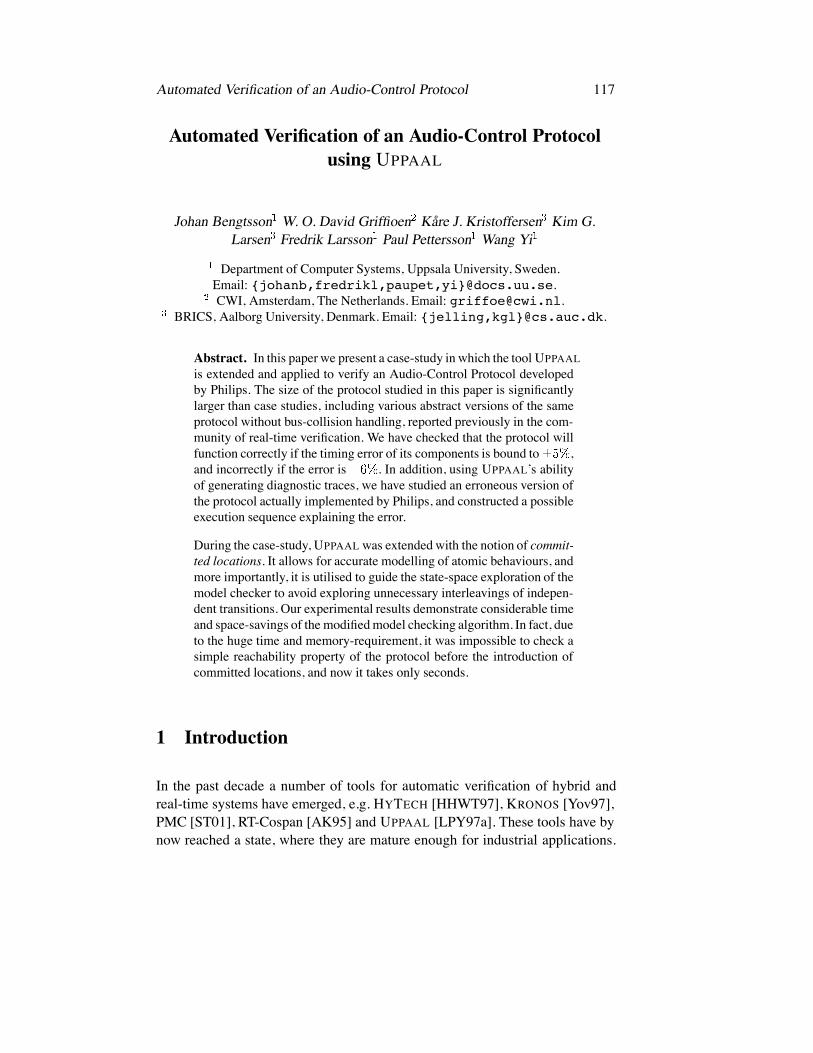
Automated Verification of an Audio-Control Protocol 117
Automated Verification of an Audio-Control Protocolusing UPPAAL
Johan Bengtsson W. O. David Griffioen Kåre J. Kristoffersen Kim G.Larsen Fredrik Larsson Paul Pettersson Wang Yi
Department of Computer Systems, Uppsala University, Sweden.Email: {johanb,fredrikl,paupet,yi}@docs.uu.se.CWI, Amsterdam, The Netherlands. Email: [email protected].
BRICS, Aalborg University, Denmark. Email: {jelling,kgl}@cs.auc.dk.
Abstract. In this paper we present a case-study in which the tool UPPAALis extended and applied to verify an Audio-Control Protocol developedby Philips. The size of the protocol studied in this paper is significantlylarger than case studies, including various abstract versions of the sameprotocol without bus-collision handling, reported previously in the com-munity of real-time verification. We have checked that the protocol willfunction correctly if the timing error of its components is bound to ,and incorrectly if the error is . In addition, using UPPAAL’s abilityof generating diagnostic traces, we have studied an erroneous version ofthe protocol actually implemented by Philips, and constructed a possibleexecution sequence explaining the error.
During the case-study, UPPAAL was extended with the notion of commit-ted locations. It allows for accurate modelling of atomic behaviours, andmore importantly, it is utilised to guide the state-space exploration of themodel checker to avoid exploring unnecessary interleavings of indepen-dent transitions. Our experimental results demonstrate considerable timeand space-savings of the modified model checking algorithm. In fact, dueto the huge time and memory-requirement, it was impossible to check asimple reachability property of the protocol before the introduction ofcommitted locations, and now it takes only seconds.
1 Introduction
In the past decade a number of tools for automatic verification of hybrid andreal-time systems have emerged, e.g. HYTECH [HHWT97], KRONOS [Yov97],PMC [ST01], RT-Cospan [AK95] and UPPAAL [LPY97a]. These tools have bynow reached a state, where they are mature enough for industrial applications.

118 Automated Verification of an Audio-Control Protocol
In this paper, we substantiate the claim by reporting on an industry-size casestudy where the tool UPPAAL is applied.
We analyse an audio control protocol developed by Philips for the physicallayer of an interface bus connecting the various devices e.g. CD-players, am-plifier etc. in audio equipments. It uses Manchester encoding to transmit bitsequences of arbitrary length between the components, whose timing errorsare bound. A simplified version of the protocol is studied by Bosscher et.al.[BPV94]. It is showed that the protocol is incorrect if the timing error of thecomponents is or greater. The proof is carried out without tool support. Thefirst automatic analysis of the protocol is reported in [HWT95] where HYTECHis applied to check an abstract version of the protocol and automatically synthe-sise the upper bound on the timing error. Similar versions of the protocol havebeen analysed by other tools, e.g. UPPAAL [LPY97a] and KRONOS [Yov97].However, all the proofs are based on a simplification on the protocol, intro-duced by Bosscher et.al. in 1994, that only one sender is transmitting on thebus so that no bus collisions can occur. In many applications the bus will havemore than one sender, and the full version of the protocol by Philips thereforehandles bus collisions. The protocol with bus collision handling was manuallyverified in [Gri94] without tool support. Since 1994, it has been a challenge forthe verification tool developers to automate the analysis on the full version ofthe protocol.
The first automated proof of the protocol with bus collision handling was pre-sented in 1996 in the conference version of this paper [BGK 96]. It was thelargest case study, reported in the literature on verification of timed systems,which has been considered as a primary example in the area (see [CW96,LSW97]). The size of the protocol studied is significantly larger than varioussimplified versions of the same protocol studied previously in the community,e.g. the discrete part of the state space (the node-space) is times larger thanin the case without bus collision handling and the number of clocks, variablesand channels in the model is also increased considerably.
The major problem in applying automatic verification tools to industrial-sizesystems is the huge time and memory-usage needed to explore the state-spaceof a network (or product) of timed automata, since the verification tools mustkeep information not only on the control structure of the automata but also onthe clock values specified by clock constraints. It is known as the state–spaceexplosion problem. We experienced the problem right on the first attempt inchecking a simple reachability property of the protocol using UPPAAL, whichdid not terminate in hours though it was installed on a super computer with giga-

Automated Verification of an Audio-Control Protocol 119
bytes of main memory. We observed that in addition to the size and complexityof the problem itself, one of the main causes to the explosion was the inaccu-rate modelling of atomic behaviours and inefficient search of the unnecessaryinterleavings of atomic behaviours by the tool. As a simple solution, duringthe case-study, UPPAAL was extended with the notion of committed locations.It allows for accurate modelling of atomic behaviours, and more importantly,it is utilised in the state-space exploration of the model checker to avoid ex-ploring unnecessary interleavings of independent transitions. Our experimentalresults demonstrate that the modified model-checking algorithm consume lesstime and space than the original algorithm. In fact, due to the huge time andmemory-requirement, it was impossible to check certain properties of the pro-tocol before the introduction of committed locations, and now it takes onlyseconds.
The automated analysis was originally carried out using an UPPAAL versionextended with the notion of committed location installed on a super computer,a SGI ONYX machine [BGK 96]. To make a comparison, in this paper wepresent an application of the current version (version 3.2) of UPPAAL, also sup-porting committed location, installed on an ordinary Pentium II 375 MHz PCmachine, to the protocol. We have checked that the protocol will function cor-rectly if the timing error of its components is bound to , and incorrectly ifthe error is . In addition, using UPPAAL’s ability of generating diagnostictraces, we have studied an erroneous version of the protocol actually imple-mented by Philips in their audio products, and constructed a possible executionsequence explaining a known error.
The paper is organised as follows: In the next two sections we present theUPPAAL model with committed location and describe its implementation in thetool. In section 4 and 5 the Philips Audio-Control Protocol with Bus Collisionis informally and formally described. The analysis of the protocol is presentedin section 6 where we also compare the performance of the current UPPAALversion with the one used in [BGK 96]. Section 7 concludes the paper. Finally,formal descriptions of the protocol components are enclosed in the appendix.
2 Committed Locations
The basis of the UPPAAL model for real-time systems is networks of timed au-tomata extended with data variables [AD90, HNSY94, YPD94]. However, tomeet requirements arising from various case-studies, the UPPAAL model has

120 Automated Verification of an Audio-Control Protocol
m1!m1!m1!m1!m1!m1!m1!m1!m1!m1!m1!m1!m1!m1!m1!m1!m1!
m2!m2!m2!m2!m2!m2!m2!m2!m2!m2!m2!m2!m2!m2!m2!m2!m2!
m1?m1?m1?m1?m1?m1?m1?m1?m1?m1?m1?m1?m1?m1?m1?m1?m1? m2?m2?m2?m2?m2?m2?m2?m2?m2?m2?m2?m2?m2?m2?m2?m2?m2?
S1S1S1S1S1S1S1S1S1S1S1S1S1S1S1S1S1 R11R11R11R11R11R11R11R11R11R11R11R11R11R11R11R11R11 R21R21R21R21R21R21R21R21R21R21R21R21R21R21R21R21R21
c:S2c:S2c:S2c:S2c:S2c:S2c:S2c:S2c:S2c:S2c:S2c:S2c:S2c:S2c:S2c:S2c:S2
S3S3S3S3S3S3S3S3S3S3S3S3S3S3S3S3S3 R12R12R12R12R12R12R12R12R12R12R12R12R12R12R12R12R12 R22R22R22R22R22R22R22R22R22R22R22R22R22R22R22R22R22
R2R2R2R2R2R2R2R2R2R2R2R2R2R2R2R2R2R1R1R1R1R1R1R1R1R1R1R1R1R1R1R1R1R1SSSSSSSSSSSSSSSSS
Figure 1: Broadcasting Communication and Committed Locations.
been extended with various new features such as urgent transitions [BLL 95]etc. The present case-study indicates that we need to further extend the UPPAALmodel with committed locations to model atomic behaviours such as multi-way synchronisations and atomic broadcasting in real-time systems. Our expe-riences with UPPAAL show that the notion of committed locations introducedin UPPAAL is not only useful in modelling but also yields significant improve-ments in performance.
We assume that a real-time system consists of a fixed number of sequentialprocesses communicating with each other via channels. We further assume thateach communication synchronises two processes as in CCS [Mil89]. Broadcast-ing communication can be implemented in such systems by repeatedly sendingthe same message to all the receivers. To ensure atomicity of such “broadcast”sequences we mark the intermediate locations of the sender, which are to beexecuted immediately, as so-called committed locations.
2.1 An Example
To introduce the notion of committed locations in timed automata, consider thescenario shown in Figure 1. A sender S is to broadcast a message m to tworeceivers R and R . As this requires synchronisation between three processesthis can not directly be expressed in the UPPAAL model, where synchronisationis between two processes with complementary actions. As an initial attempt wemay model the broadcast as a sequence of two two-process synchronisations,

Automated Verification of an Audio-Control Protocol 121
where first S synchronises with R on m and then with R on m . However,this is not an accurate model as the intended atomicity of the broadcast is notpreserved (i.e. other processes may interfere during the broadcast sequence).To ensure atomicity, we mark the intermediate location S of the sender S asa committed location (indicated by the c:-prefix). The atomicity of the actionsequence m !m ! is now achieved by insisting that a committed sequence mustbe left immediately! This behaviour is similar to what has been called “urgenttransitions” [HHWT95, DY95, BLL 95], which insists that the next transitiontaken must be an action (and not a delay), but the essential difference is thatno other actions should be performed in between such an atomic sequence. Theprecise semantics of committed locations will be formalised in the transitionrules for networks of timed automata with data variables in Section 2.3.
2.2 Syntax
We assume a finite set of clock variables ranged over by and a finiteset of data variables ranged over by . We use to stand for the set ofclock constraints that are the conjunctive formulas of simple constraints in theform of or , where and is a naturalnumber. Similarly, we use to stand for the set of non-clock constraintsthat are conjunctive formulas of or , whereand is an integer number. We use ranged over by to denote the set offormulas that are conjunctions of clock constraints and a non-clock constraints.The elements of are called constraints or guards.
To manipulate clock and data variables, we use reset-sets which are finite setsof reset-operations. A reset-operation on a clock variable should be in the form
where is a natural number and a reset-operation on an data variableshould be in the form: where are integers. A reset-set is aproper reset-set when the variables are assigned a value at most once, we use
to denote the set of all proper reset-sets.
We assume that processes synchronise with each other via complementary ac-tions. Let be a set of action names with a subset of urgent actions on whichprocesses should synchronise whenever possible. We use ct
to denote the set of actions that processes canperform to synchronise with each other, where is a distinct symbol represent-ing internal actions. We use name to denote the action name of , defined byname name .

122 Automated Verification of an Audio-Control Protocol
An automaton over actions ct, clock variables and data variables is atuple where is a finite set of locations (control-locations)with a subset being the set of committed locations, is the initiallocation, ct corresponds to the set of edges,and is the invariant assignment function. To model urgency, werequire that the guard of an edge with an urgent action is a non-clock constraint,i.e. if name and then .
In the case, we shall write which represents a transi-tion from the location to the location with guard , action to be performed,and a sequence of reset-operations to update the variables. Furthermore, weshall write whenever .
To model networks of processes, we introduce a CCS-like parallel composi-tion operator for automata. Assume that are automata. We use todenote their parallel composition. The intuitive meaning of is similar to theCCS parallel composition of with all actions being restricted, thatis, ct. Thus only synchronisation between the components
is possible. We call a network of automata. We simply view as a vectorand use to denote its th component.
2.3 Semantics
Informally, a process modelled by an automaton starts at location with all itsvariables initialised to . The values of the clocks may increase synchronouslywith time at location as long as the invariant condition is satisfied. At anytime, the process can change location by following an edge providedthe current values of the variables satisfy the enabling condition . With thistransition, the variables are updated by .
To formalise the semantics we shall use variable assignments. A variable as-signment is a mapping which maps clock variables to the non-negative realsand data variables to integers. For a variable assignment and a delay ,
denotes the variable assignment such that for aclock variable and for any data variable . This definition of
reflects that all clocks proceed at the same speed and that data variables aretime-insensitive.
For a reset-set (a proper set of reset-operations), we use to denote thevariable assignment with Value whenever and
otherwise, where Value denotes the value of in . Given

Automated Verification of an Audio-Control Protocol 123
a constraint and a variable assignment , is a boolean valuedescribing whether is satisfied by or not.
A control vector of a network is a vector of locations where is a locationof . We write to denote the vector where the th element of isreplaced by . Furthermore, we shall write whenever for some .
A state of a network is a configuration where is a control vector ofand is a variable assignment. The initial state of is where is theinitial control vector whose elements are the initial locations of ’s andis the initial variable assignment that maps all variables to .
The semantics of a network of automata is given in terms of a transitionsystem with the set of states being the configurations. The transition relation isdefined by the following three rules, which are standard except that each rulehas been augmented with conditions handling control-vectors with committedlocations:
if and for some , , , and forall if then .
if , , ,, and , for some , , , , , , and for all if
then or .
if , , and no ,such that , , , , , and .
where .
Intuitively, the first rule describes a local internal action transition in a compo-nent, and possibly the resetting of variables. An internal transition can occur ifthe current variable assignment satisfies the transition guard and if the control-location of any component is committed, only components in committed loca-tions may take local transitions. Thus, only internal transitions of componentsin committed location may interrupt other components operating in committedlocations.
The second rule describes synchronisation transitions that synchronise two com-ponents. If the control-location of any of the components is committed it isrequired that at least one of the synchronising components starts in a commit-ted location. This requirement prevents transitions starting in non-committed

124 Automated Verification of an Audio-Control Protocol
locations from interfering with atomic (i.e. committed) transition sequences.However, two independent committed sequences may interfere with each other.
The third rule describes delay transitions, i.e. when all clocks increase syn-chronously with time. Delay transitions are permitted only while the location in-variants of all components are satisfied. Delays are not permitted if the control-location of a component in the network is committed, or if an urgent transition(i.e. a synchronisation transition with urgent action) is possible. Note that theguards on urgent transitions are non-clock constraints whose truth-values arenot affected by delays.
Finally, we note that the three rules give a semantics where transition sequencesmarked as committed are instantaneous in the sense that they happen withoutduration, and without interference from components operating in non-committedlocations.
3 Committed Locations in UPPAAL
In this section we present a modified version of the model-checking algorithmof UPPAAL for networks of automata with committed locations.
3.1 The Model-Checking Algorithm
The model-checking algorithm performs reachability analysis to check for in-variance properties , and reachability properties , with respect to alocal property of the control locations and the values of the clock and datavariables1. It combines symbolic techniques with on-the-fly generation of thestate-space in order to avoid explicit construction of the product automaton andthe immediately caused memory problems. The algorithm is based on a parti-tioning of the (otherwise infinite) state-space into finitely many symbolic statesof the form , where is a constraint system (i.e. a conjunction of clockconstraints and non-clock constraints). It checks if a any part of a symbolicstate (i.e. a state with ) is reachable from the initialsymbolic state , where expresses that all clock and data variablesare initialised to [YPD94]. Throughout the rest of this paper we shall simplycall a state instead of symbolic state.
1From version 3.2 released in 2001, the model-checking algorithm in UPPAAL also supportsliveness properties of the kind and .

Automated Verification of an Audio-Control Protocol 125
The algorithm essentially performs a forwards search of the state-space. Thesearch is guided and pruned by two buffers: WAITING, holding states waitingto be explored and PASSED holding states already explored. Initially, PASSED isempty and WAITING holds the single state . The algorithm then repeatsthe following steps:
S1. Pick a state from the WAITING buffer.
S2. If and return the answer yes.
S3. a. If and , for some in the PASSED buffer, dropand go to step S1.
b. Otherwise, save in the PASSED buffer.
S4. Find all successor states reachable from in one step andstore them in the WAITING buffer.
S5. If the WAITING buffer is not empty then go to step S1, otherwise returnthe answer no.
We will not treat the algorithm in detail here, but refer the reader to [YPD94,BL96].
Note that in step S3.b all explored states are stored in the PASSED buffer toensure termination of the algorithm. In many cases, it will store the whole state-space of the analysed system which grows exponentially both in the numberclocks and components [YPD94]. The algorithm is therefore bound to run intospace problems for large systems. The key question is how to reduce the growthof the PASSED buffer.
When committed locations are used to model atomic behaviours there are twopotential possibilities to reduce the size of the PASSED buffer. First, as atomicsequences in general restrict the amount of interleaving that is allowed in a sys-tem [Hol91], the state-space of the system is reduced, and consequently also thenumber of states stored in the PASSED buffer. Secondly, as a sequence of com-mitted locations semantically is instantaneous and non-interleaved with othercomponents, it suffices to save only the (non-committed) control-location at thebeginning of the sequence in the PASSED buffer to ensure termination. Hence,our proposed solution is simply not to save states in the PASSED buffer whichinvolve committed locations. We modify step S3 of the algorithm in the follow-ing way:

126 Automated Verification of an Audio-Control Protocol
Dj2Dj2Dj2Dj2Dj2Dj2Dj2Dj2Dj2Dj2Dj2Dj2Dj2Dj2Dj2Dj2Dj2
k==nk==nk==nk==nk==nk==nk==nk==nk==nk==nk==nk==nk==nk==nk==nk==nk==na!a!a!a!a!a!a!a!a!a!a!a!a!a!a!a!a!
a!a!a!a!a!a!a!a!a!a!a!a!a!a!a!a!a!k:=k+1k:=k+1k:=k+1k:=k+1k:=k+1k:=k+1k:=k+1k:=k+1k:=k+1k:=k+1k:=k+1k:=k+1k:=k+1k:=k+1k:=k+1k:=k+1k:=k+1
k:=1k:=1k:=1k:=1k:=1k:=1k:=1k:=1k:=1k:=1k:=1k:=1k:=1k:=1k:=1k:=1k:=1
S3S3S3S3S3S3S3S3S3S3S3S3S3S3S3S3S3
c:S2c:S2c:S2c:S2c:S2c:S2c:S2c:S2c:S2c:S2c:S2c:S2c:S2c:S2c:S2c:S2c:S2
S1S1S1S1S1S1S1S1S1S1S1S1S1S1S1S1S1
SSSSSSSSSSSSSSSSS
Dj1Dj1Dj1Dj1Dj1Dj1Dj1Dj1Dj1Dj1Dj1Dj1Dj1Dj1Dj1Dj1Dj1
DjDjDjDjDjDjDjDjDjDjDjDjDjDjDjDjDj
i==ki==ki==ki==ki==ki==ki==ki==ki==ki==ki==ki==ki==ki==ki==ki==ki==ka?a?a?a?a?a?a?a?a?a?a?a?a?a?a?a?a?
Ri1Ri1Ri1Ri1Ri1Ri1Ri1Ri1Ri1Ri1Ri1Ri1Ri1Ri1Ri1Ri1Ri1
Ri2Ri2Ri2Ri2Ri2Ri2Ri2Ri2Ri2Ri2Ri2Ri2Ri2Ri2Ri2Ri2Ri2
RiRiRiRiRiRiRiRiRiRiRiRiRiRiRiRiRi
Figure 2: Broadcasting Using Committed Locations.
S3 . a. If go directly to step S4.
b. If and , for some in the PASSED buffer, dropand go to step S1.
c. If neither of the above steps are applicable, save in the PASSEDbuffer.
So, for a given state , if is committed the algorithm proceeds directlyfrom step S3 .a to step S4, thereby omitting the time-consuming step S3 .band the space-consuming step S3 .c. Clearly, this will reduce the growth of thePASSED buffer and the total amount of time spent on step S3 . In the followingstep S4 more reductions are made as interleavings are not allowed when iscommitted. In fact, the next transition must be an action transition and it mustinvolve a which is committed in (according to the transition rules in theprevious section). This reduces the time spent on generating successor statesof in S4 as well as the total number of states in the system. Finally, wenote that reducing the PASSED buffer size also yields potential time-savings instep S3 .b when is not committed as it involves a search through the PASSEDbuffer.
It should be noticed that the algorithm presented in this section is not guaranteedto terminate if the notion of committed locations is used in an unintended way2.For the modified algorithm to terminate, it is assumed in the that committedlocations are used to model atomic behaviours. In particular this means thatany sequence of committed control-locations must be of finite length.
2In the current implementation of UPPAAL, the algorithm uses a technique presented in[LLPY97] to identify and store at least one so-called covering state in each dynamic loop toguarantee termination for all input models.

Automated Verification of an Audio-Control Protocol 127
Receivers
Tim
e (s
ec.)
70
60
50
40
30
20
10
1 2 3 4 5
S2 not commitedS2 commited
360
350
340
330
320
310
300
S2 not commitedS2 commited
54321
380
370
Receivers
Spac
e (p
ages
)
Figure 3: Time and Space Consumption.
3.2 Space and Time Performance Improvements
To investigate the practical benefits from the usage of committed locations andits implementation in UPPAAL we perform an experiment with a parameteris-able scenario, where a sender S wants to broadcast a message to receiversR R . The sender S simply performs a!-transitions and then termi-nates, whereas the receivers are all willing to perform a single a?-transitionhereby synchronising with the sender. The data variable k ensures that the threceiver participates in the th handshake. Additionally, there are auxiliaryautomata D D simply oscillating between two states. Consider Figure 2,where the control node S is committed (indicated by the c:-prefix).
We may now use UPPAAL to verify that the sender succeeds in broadcasting themessage, i.e. it forces all the receivers to terminate. More precisely we verifythat SYS S R R D D satisfies the formula
at(S,S ) at(R ,R ) , where we assume that the proposition at( , )is implicitly assigned to each location of the automaton , meaning that thecomponent is operating in location . We perform two verifications, one withS declared as committed, and one with S being non-committed but with alocation invariant , where x is a clock which is reset on the transitionfrom S1 to S2, preventing the automaton from delaying in location S . Theresult is shown in Figure 3. In both test sequences the number of disturbingautomata was fixed to eight. Time is measured in seconds and space is measuredin pages (4KB). The general observation is that use of committed locations inbroadcasting saves time as well as space. The most important observation is

128 Automated Verification of an Audio-Control Protocol
that in the committed scenario the space consumption behaves as a constantfunction in the number of receivers.
4 The Audio Control Protocol with Bus Collision
In this section an informal introduction to the audio protocol with bus collisionis given. The audio control protocol is a bus protocol, all messages are receivedby all components on the bus. If a component receives a message not addressedto it, the message is just ignored. Philips allows up to 10 components.
Messages are transmitted using Manchester encoding. Time is divided into bit-slots of equal length, a bit “1” is transmitted by an up-going edge halfway abit-slot, a bit “0” by a down-going edge halfway a bit-slot. If the same bit istransmitted twice in a row the voltage must of course change at the end of thefirst bit-slot. Note that only a single wire is used to connect the components, noextra clock wire is needed. This is one of the properties that makes it a usefulprotocol.
The protocol has to cope with some problems: The sender and the receivermust agree on the beginning of the first bit-slot, the length of the message isnot known in advance by the receiver, the down-going edges are not detectedby the receiver. To resolve these problems the following is required: Messagesmust start with a bit “1” and messages must end with a down-going edge. Thisensures that the voltage on the wire is low between messages. Furthermore thesenders must respect a so-called “radio silence” between the end of a messageand the beginning of the next one. The radio silence marks the end of a mes-sage and the receiver knows that the next up-going edge is the first edge of anew message. It is almost possible, and actually mandated in the Philips doc-umentation, to decode a Manchester encoded message by only looking to theup-going edges (problem ) only the last zero bit of a message can not be de-tected (consider messages “10” and “1”). To resolve this, it is required that allmessages are of odd length.
It is possible that two or more components start transmitting at the same time.The behaviour of the electric circuit is such that the voltage on the wire willbe high as long as one of the senders pulls it high. In other words: The wireimplements the or-function. This makes it possible for a sender to notice thatsomeone else is also transmitting. If the wire is high while it is transmittinga low, a sender can detect a bus collision. This collision detection happens atcertain points in time: Just before each up-going transition, and at one and three

Automated Verification of an Audio-Control Protocol 129
Figure 4: An Example.
quarters of a bit-slot after a down going edge (if it is still transmitting a low).When a sender detects a collision it will stop transmitting and will try to re-transmit its message later.
If two messages are transmitted at the same time and one is a prefix of the other,the receiver will not notice the prefix message. To ensure collision detection itis not allowed that a message is a prefix of another message in transit. In thePhilips environment this restriction is met by embedding the source address ineach message (and assigning each component a unique source address).
In Figure 4 an example is depicted. Assume two senders, named A and B,that start transmitting at exactly the same time. Because two lines on top ofeach other are hard to distinguish from one line, in the picture they are shiftedslightly. The sender A (depicted with thick lines) starts transmitting “11...” andsender B (depicted with thin lines) “101...”. At the end of the first bit-slotsender A changes from high to low voltage, to prepare for the next up-goingedge. But one quarter after this down it detects a collision and stops transmit-ting. Sender B did not notice the other sender and continues transmitting. Notethat the receiver will decode the message of the sender B correctly.
The protocol has to cope with one more thing: timing uncertainty. Becausethe protocol is implemented on a processor that also has to execute a numberof other time critical tasks, a quite large timing uncertainty is allowed. A bit-slot is 888 microseconds, so the ideal time between two edges is 888 or 444microseconds. On the generation of edges a timing uncertainty of 5% is al-lowed. That is, between 844 and 932 for one bit-slot and between 422 and 466for half a bit-slot. The collision detection just before an up-going edge and theactual generation of the same up-going edge should be separated by at most 20microseconds (according to the protocol specification). The timing uncertaintyon the collision detection appearing at the first and third quarters after a down-going edge is 22 microseconds. Also the receiver has a timing uncertainty of
5%. To complete the timing information, the distance between the end of onemessage and the beginning of the next must be at least 8000 microseconds (8milliseconds).

130 Automated Verification of an Audio-Control Protocol
Add0
Add1
OUT
(Ax,Ad,Anext)
SenderA
(Bx,Bd,Bnext)
SenderB
Bhead0
Bhead1
Bempty
Ahead0
Ahead1
Aempty
(Volt,w)
(Volt,w)
UP,DOWN
UP,DOWN
VUP,(w)
(odd)
(r,l)
AINc,expect0,expect1,CAcoll,(as)
Wire Receiver
Check
Acoll
Bcoll
(ok)
(Bod,Blb,bs)
MessageB
(od,lb)
MessageA
Figure 5: Philips Audio-Control Protocol with Bus Collision.
5 A Formal Model of the Protocol
To analyse the behaviour of the protocol we model the system as a networkof seven timed automata. The network consists of two parts: a core part and atesting environment. The core part models the components of the protocol to beimplemented: two senders, a wire and a receiver. The testing environment, con-sisting of two message generators (one for each sender) and an output checker,is used to model assumptions about the environment of the protocol and fortesting the behaviour of the core part. Figure 5 shows a flow-graph of the net-work where nodes represent timed automata and edges represent synchronisa-tion channels or shared variables, the latter enclosed within parentheses.
The general idea of the model is as follows. The two automata MessageA andMessageB are designed to non-deterministically generate possible valid mes-sages for the both senders (as described in section 4), in additionMessageA in-forms the Check-automaton on the bits it generated for SenderA. The senderstransmit the messages via the wire to the receiver. We have chosen to modelthe wire as an automaton to separate its behaviour from the two senders and thereceiver. The receiver communicates the bits it decoded to the checker. Thusthe Check automaton is able to compare the bits generated by MessageA andthe bits received by Receiver. If this matches the protocol is correct.
The senders A and B are, modulo renaming (all A’s in identifiers to B’s), exactlythe same. Because of the symmetry, it is enough to check that the messagestransmitted by sender A are received correctly. If a scenario exits in which amessage of sender B is received incorrectly, the same scenario (modulo re-naming) exists for sender A. We will proceed with a short description of each

Automated Verification of an Audio-Control Protocol 131
automaton. The definition of these uses a number of constants that are declaredin Table 1 in Appendix 8.
The Senders
SenderA is depicted in Figure 10. It takes input actions Ahead0?, Ahead1?and Aempty?. The output actions UP! and DOWN! will be the Manchesterencoding of the message. The clock Ax is used to measure the time betweenUP! and DOWN! actions. The idea behind the model (taken from [DY95]) isthat the sender changes location each half of a bit-slot. The locations HS (wireis High in Second half of the bit-slot) and HF (High in First half of the bit-slot)refer to this idea. Extra locations are needed because of the collision detection.
The clock Ad is used to measure the time elapsed between the detection justbefore UP! action and the corresponding UP! action. The system is in the loca-tions ar_Qfirst and ar_Qlast when the next thing to do is the collision test atone or three quarters of a bit-slot. When Volt is greater than zero, at that mo-ment, the sender detects a collision, stops transmitting and returns to the idlelocation. The clock w is used to ensure the radio silence between messages.This variable is checked on the transition from idle to ar_first_up.
The Wire
This small automaton keeps track of the voltage on the wire and generates VUP!actions when appropriate, that is when a UP? action is received when the volt-age is low. The automaton is shown in Figure 9.
The Receiver
Receiver, shown in Figure 8, decodes the bit sequence using the up-going(modelled as VUP?) changes of the wire. Decoded bits are signalled to theenvironment using output actions Add0!, Add1! and OUT! (where OUT! isused for signalling the end of a decoded message). The decoding algorithm ofthe receiver is a direct translation of the algorithm in the Philips documenta-tion of the protocol. In the automaton each VUP? transition is followed by atransition modelling the decoding. This decoding happens at once, thereforethe intermediate locations are modelled as committed locations. The automatonhas two important locations, L1 and L0. When the last received bit is a bit “1”the receiver is in location L1, after receiving a bit “0” it will be in location L0.The error location is entered when a VUP? is received much too early. In thecomplete model the error location is not reachable, see Section 6. The receiver

132 Automated Verification of an Audio-Control Protocol
keeps track of the parity of the received message using the integer variable odd.When the last received bit is a bit “1” and the message is even, a bit “0” is addedto make the complete message of odd length.
The Message Generators
The message generators MessageA andMessageB, shown in Figure 11, gen-erate valid messages (i.e. any message for which the protocol should behavecorrectly according to the specification) for sender A and B. In addition, themessages generated for sender A are communicated to the checker. The start ofa message is signalled to the checker by AINc!, bits by expect0! and expect1!.When a collision is detected by sender A this is communicated to MessageAvia Acoll?. The message generator will communicate this on his turn to thecheck automaton via CAcoll!.
Generating messages of odd length is quite simple. The only problem is that itis not allowed that a message for one sender is a prefix of the message for theother sender. To be more precise: If only one sender is transmitting there is noprefix restriction. Only when the two senders start transmitting at the same time,it is not allowed that one sender transmits a prefix of the message transmittedby the other. As mentioned before the reason for this restriction is that the prefixmessage is not received by the receiver and it is possible that the senders do notnotice the collision. In other words: the prefix message can be lost. To ensurethat the two generated bit-streams differ on at least on position, the generatoralways compare the last generated bit-values stored in the variables lb and Blbon the edge from locations sending0 or sending1 to location sending. If thebits differ, the variable ok is set to 1, which is a requirement for the messagegeneration to end normally (on the transition from sending to idle in the twoautomata).
The Checker
This automaton is shown in Figure 7. It keeps track of the bits “in transit”,i.e. the bits that are generated by the message generators but not yet decodedby the receiver. These bits are encoded using the two variables l, which storesthe length of the bit-stream, and r that stores the actual bit-stream in transit.Whenever a bit is decoded or the end of the message is detected not conformthe generated message the checker enters location error. Furthermore, whensender A detects a collision the checker returns to its initial location.

Automated Verification of an Audio-Control Protocol 133
6 Verification in UPPAAL
In this section we present the results of analysing the Philips audio-control pro-tocol formally described in the previous section. We will use to denote the(implicit) proposition at( ) introduced in Section 3.2. Also, note that invari-ance properties in UPPAAL are on the form , where is a local property.
Correctness Criteria
The main correctness criterion of the protocol is to ensure that the bit sequencereceived by the Receiver matches the bit sequence sent by SenderA. More-over, the entire bit sequence should be received by Receiver (and communi-cated to Check). From the description of the Check-automaton (see the previ-ous section) it follows that this behaviour is ensured if Check is always operat-ing in location start or normal:
Check start Check normal (1)
When theReceiver-automaton observes changes of the wire too early it changescontrol to location error. If the rest of the components behave normally thisshould not happen. Therefore, the Receiver-automaton is required to neverreach the location error:
Receiver error (2)
Incorrectness
Unfortunately the protocol described in this paper is not the protocol that Philipshas implemented. The original sender checked less often for a bus collision. The“just before the up going edge” collision detection was only performed beforethe first up. In the UPPAAL model this corresponds to deleting outgoing transi-tions of ar_Qlast_ok and using the outgoing transitions of ar_up_ok instead.This incorrect version is shown in Figure 12. In general the problem is that ifboth senders are transmitting and one is slow and the other fast, the distancecan cumulate to a high value that can confuse the receiver. UPPAAL generated acounter-example trace to Property 1. The trace is depicted in Figure 6. The sce-nario is as follows: Sender A (depicted with thick lines) tries to transmit “111...”and sender B (depicted with thin lines) “1100...”. The sender A is fast and theother slow. This causes the distance between the second UP’s to be very big (77microseconds). In the third bit-slot the sender A detects the collision. The resultof all this is that the time elapsed between the VUP actions is 6.65Q instead of

134 Automated Verification of an Audio-Control Protocol
first bitslot ideal distance = 6Qactual distance = 6.65Q
Figure 6: Error execution of the incorrect protocol.
the ideal 6Q. Because of the timing uncertainty in the receiver this can be inter-preted as 7Q ( ), and 7Q is just enough to decode “01” insteadof the transmitted “0”. Thus, it is possible that the sent and received messagediffer with this version of the protocol.
In the correct version this scenario is impossible, because if collision detectionhappens before every UP action, the distance between the UP’s in the secondbit-slot can not be that high (at most 20 microseconds).
It is not likely that these kind of errors happen in the actual implementation.First, it is not likely that two senders do start at sufficiently close time-points.Secondly, the timing uncertainty is at most 2% instead of 5%, and the “average”timing uncertainty is even less. For more details, see [Gri94].
Although this problem was known by Philips it is interesting to see how pow-erful the diagnostic traces can be. It enables us not only to find mistakes in themodel of a protocol, but also to find design mistakes in real-life protocols.
Verification Results
UPPAAL successfully verifies the correctness properties 1 and 2 for an errortolerance of 5% on the timing. Recall that SenderA and SenderB are, modulorenaming, exactly the same, implying that the verified properties for SenderAalso applies to the symmetric case for SenderB. The verification of Property 1and 2 was performed in 0.5 sec using 2.5 MB of memory.
The analysis of the incorrect version of the protocol with less collision detection(discussed above) uses UPPAAL’s ability to generate diagnostic traces wheneveran invariant property is not satisfied by the system. The trace, consisting of 46transitions, was generated in 0.4 sec using 2.5 MB of memory. Also, verificationof Property 1 for the protocol with full collision detection and an error tolerance

Automated Verification of an Audio-Control Protocol 135
of 6% on all the timing produces an error trace as well. The scenario is similarto the one found by Bosscher et.al. in [BPV94] for the one sender protocol.
The properties were verified using UPPAAL version 3.2 [LPY97a, BLL 98,ABB 01] that implements the verification algorithm handling committed lo-cations described in Section 3. It was installed on a Pentium II 375 MHz PCrunning Debian Linux 2.2. In the conference version of this paper [BGK 96]we reported that the same protocol was verified using UPPAAL version 0.963
installed on a SGI ONYX machine. The verification of the two correctnessproperties then consumed 7.5 hrs using 527.4 MB and 1.32 hrs using 227.9MB, whereas a diagnostic trace for the incorrect version was generated in 13.0min using 290.4 MB of memory. Hence, both the time- and space-consumptionof the verifier for this particular model have been reduced with over 99%. Theseimprovements of the UPPAAL verifier are due to a number of developments inthe last years that will not be discussed further here. It should also be noticedthat the older version uses backwards analysis whereas the newer performs for-wards analysis. For more information he developments of UPPAAL we refer thereader to [LPY97b, BLL 98, ABB 01].
7 Conclusions
In this paper we have presented a case-study where the verification tool UPPAALis used to verify an industrial audio-control protocol with bus-collision handlingby Philips. The protocol has received a lot of attention in the formal methodsresearch community (see e.g. [BPV94, HWT95, CW96]) and simplified ver-sions of the protocol without the handling of bus collisions have previously beenanalysed by several research teams, with and without support from automatictools.
As verification results we have shown that the protocol behaves correctly if theerror on all timing is bound to 5%, and incorrectly if the error is 6%. Fur-thermore, using UPPAAL’s ability to generate diagnostic traces we have beenable to study error scenarios in an incorrect version of the protocol actuallyimplemented by Philips.
In this paper we have also introduced the notion of so-called committed loca-tions which allows for more accurate modelling of atomic behaviours. Moreimportantly, it is also utilised to guide the state-space exploration of the model
3The two UPPAAL versions 0.96 and 2.17 are dated Nov 1995 and March 1998 respectively.

136 Automated Verification of an Audio-Control Protocol
checker to avoid exploring unnecessary interleavings of independent transi-tions. Our experimental results demonstrate considerable time and space-savingsof the modified model checking algorithm. In fact, due to the huge time andmemory-requirement, it was impossible to check certain properties of the pro-tocol before the introduction of committed locations, and now it takes onlyseconds.
References
[ABB 01] Tobias Amnell, Gerd Behrmann, Johan Bengtsson, Pedro R. D’Argenio,Alexandre David, Ansgar Fehnker, Thomas Hune, Bertrand Jeannet,Kim G. Larsen, M. Oliver Möller, Paul Pettersson, Carsten Weise, andWang Yi. UPPAAL - Now, Next, and Future. In F. Cassez, C. Jard,B. Rozoy, and M. Ryan, editors, Modelling and Verification of ParallelProcesses, number 2067 in Lecture Notes in Computer Science, pages100–125. Springer–Verlag, 2001.
[AD90] Rajeev Alur and David Dill. Automata for Modelling Real-Time Systems.In Proc. of Int. Colloquium on Algorithms, Languages and Programming,number 443 in Lecture Notes in Computer Science, pages 322–335, July1990.
[AK95] Rajeev Alur and Robert P. Kurshan. Timing Analysis in COSPAN. InRajeev Alur, Thomas A. Henzinger, and Eduardo D. Sontag, editors,Proc.of Workshop on Verification and Control of Hybrid Systems III, number1066 in Lecture Notes in Computer Science, pages 220–231. Springer–Verlag, October 1995.
[BGK 96] Johan Bengtsson, W.O. David Griffioen, Kåre J. Kristoffersen, Kim G.Larsen, Fredrik Larsson, Paul Pettersson, and Wang Yi. Verification of anAudio Protocol with Bus Collision Using UPPAAL. In Rajeev Alur andThomas A. Henzinger, editors, Proc. of the 8th Int. Conf. on ComputerAided Verification, number 1102 in Lecture Notes in Computer Science,pages 244–256. Springer–Verlag, July 1996.
[BL96] Johan Bengtsson and Fredrik Larsson. UPPAAL a Tool for AutomaticVerification of Real-time Systems. Master’s thesis, Uppsala Univer-sity, 1996. Available as http://www.docs.uu.se/docs/rtmv/-bl-report.pdf.
[BLL 95] Johan Bengtsson, Kim G. Larsen, Fredrik Larsson, Paul Pettersson, andWang Yi. UPPAAL — a Tool Suite for Automatic Verification of Real–Time Systems. In Proc. of Workshop on Verification and Control of Hy-brid Systems III, number 1066 in Lecture Notes in Computer Science,pages 232–243. Springer–Verlag, October 1995.

Automated Verification of an Audio-Control Protocol 137
[BLL 98] Johan Bengtsson, Kim G. Larsen, Fredrik Larsson, Paul Pettersson, WangYi, and Carsten Weise. New Generation of UPPAAL. In Int. Workshop onSoftware Tools for Technology Transfer, June 1998.
[BPV94] D. Bosscher, I. Polak, and F. Vaandrager. Verification of an Audio-ControlProtocol. In Proc. of Formal Techniques in Real-Time and Fault-TolerantSystems, number 863 in Lecture Notes in Computer Science, 1994.
[CW96] Edmund M. Clarke and Jeanette M. Wing. Formal Methods: State ofthe Art and Future Directions. ACM Computing Surveys, 28(4):626–643,December 1996.
[DY95] C. Daws and S. Yovine. Two examples of verification of multirate timedautomata with KRONOS. In Proc. of the 16th IEEE Real-Time SystemsSymposium, pages 66–75. IEEE Computer Society Press, December 1995.
[Gri94] W.O. David Griffioen. Analysis of an Audio Control Protocol with BusCollision. Master’s thesis, University of Amsterdam, Programming Re-search Group, 1994.
[HHWT95] Thomas A. Henzinger, Pei-Hsin Ho, and Howard Wong-Toi. HYTECH:The Next Generation. In Proc. of the 16th IEEE Real-Time Systems Sym-posium, pages 56–65. IEEE Computer Society Press, December 1995.
[HHWT97] Thomas A. Henzinger, Pei-Hsin Ho, and Howard Wong-Toi. HYTECH:A Model Checker for Hybrid Systems. Int. Journal on Software Tools forTechnology Transfer, 1(1–2):134–152, October 1997.
[HNSY94] Thomas. A. Henzinger, Xavier Nicollin, Joseph Sifakis, and SergioYovine. Symbolic Model Checking for Real-Time Systems. Informationand Computation, 111(2):193–244, 1994.
[Hol91] Gerard Holzmann. The Design and Validation of Computer Protocols.Prentice Hall, 1991.
[HWT95] Pei-Hsin Ho and Howard Wong-Toi. Automated Analysis of an AudioControl Protocol. In Proc. of the 7th Int. Conf. on Computer Aided Ver-ification, number 939 in Lecture Notes in Computer Science. Springer–Verlag, 1995.
[LLPY97] Fredrik Larsson, Kim G. Larsen, Paul Pettersson, and Wang Yi. EfficientVerification of Real-Time Systems: Compact Data Structures and State-Space Reduction. In Proc. of the 18th IEEE Real-Time Systems Sympo-sium, pages 14–24. IEEE Computer Society Press, December 1997.
[LPY97a] Kim G. Larsen, Paul Pettersson, and Wang Yi. UPPAAL in a Nutshell.Int. Journal on Software Tools for Technology Transfer, 1(1–2):134–152,October 1997.

138 Automated Verification of an Audio-Control Protocol
[LPY97b] Kim G. Larsen, Paul Pettersson, and Wang Yi. UPPAAL: Status and De-velopments. In Orna Grumberg, editor, Proc. of the 9th Int. Conf. onComputer Aided Verification, number 1254 in Lecture Notes in ComputerScience, pages 456–459. Springer–Verlag, June 1997.
[LSW97] Kim G. Larsen, Bernard Steffen, and Carsten Weise. Continuous mod-eling of real-time and hybrid systems: from concepts to tools. Int. Jour-nal on Software Tools for Technology Transfer, 1(1–2):64–85, December1997.
[Mil89] R. Milner. Communication and Concurrency. Prentice Hall, EnglewoodCliffs, 1989.
[ST01] R. F. Lutje Spelberg and W. J. Toetenel. Parametric real-time modelchecking using splitting trees. Nordic Journal, 8(1):88–120, 2001.
[Yov97] Sergio Yovine. A Verification Tool for Real Time Systems. Int. Journal onSoftware Tools for Technology Transfer, 1(1–2):134–152, October 1997.
[YPD94] Wang Yi, Paul Pettersson, and Mats Daniels. Automatic Verification ofReal-Time Communicating Systems By Constraint-Solving. In DieterHogrefe and Stefan Leue, editors, Proc. of the 7th Int. Conf. on FormalDescription Techniques, pages 223–238. North–Holland, 1994.

Automated Verification of an Audio-Control Protocol 139
8 Appendix
The constants used in the formulasq 2220 One quarter of a bit-slot: 222 micro secd 200 Detection ’just before’ the UP:
20 micro secg 220 ’Around’ 25% and 75% of the bit-slot:
22 micro secw 80000 The radio silence: 8 milli sect 0.05 The timing uncertainty: 5%The constants in the automataW w 80000D d 200A1min q-g 2000A1max q+g 2440A2min 3*q-g 6440A2max 3*q+g 6880Q2 2*q 4440Q2minD 2*q*(1-t)-d 4018Q2min 2*q*(1-t) 4218Q2max 2*q*(1+t) 4662Q3min 3*q*(1-t) 6327Q3max 3*q*(1+t) 6993Q5min 5*q*(1-t) 10545Q5max 5*q*(1+t) 11655Q7min 7*q*(1-t) 14763Q7max 7*q*(1+t) 16317Q9min 9*q*(1-t) 18981Q9max 9*q*(1+t) 20979
Table 1: Declaration of Constants.

140 Automated Verification of an Audio-Control Protocol
checkcheckcheckcheckcheckcheckcheckcheckcheckcheckcheckcheckcheckcheckcheckcheckcheck
startstartstartstartstartstartstartstartstartstartstartstartstartstartstartstartstart
normalnormalnormalnormalnormalnormalnormalnormalnormalnormalnormalnormalnormalnormalnormalnormalnormal
errorerrorerrorerrorerrorerrorerrorerrorerrorerrorerrorerrorerrorerrorerrorerrorerror
OUT?OUT?OUT?OUT?OUT?OUT?OUT?OUT?OUT?OUT?OUT?OUT?OUT?OUT?OUT?OUT?OUT?as==0as==0as==0as==0as==0as==0as==0as==0as==0as==0as==0as==0as==0as==0as==0as==0as==0
Add1?Add1?Add1?Add1?Add1?Add1?Add1?Add1?Add1?Add1?Add1?Add1?Add1?Add1?Add1?Add1?Add1?as==0as==0as==0as==0as==0as==0as==0as==0as==0as==0as==0as==0as==0as==0as==0as==0as==0
Add0?Add0?Add0?Add0?Add0?Add0?Add0?Add0?Add0?Add0?Add0?Add0?Add0?Add0?Add0?Add0?Add0?as==0as==0as==0as==0as==0as==0as==0as==0as==0as==0as==0as==0as==0as==0as==0as==0as==0
AINc?AINc?AINc?AINc?AINc?AINc?AINc?AINc?AINc?AINc?AINc?AINc?AINc?AINc?AINc?AINc?AINc?r:=1r:=1r:=1r:=1r:=1r:=1r:=1r:=1r:=1r:=1r:=1r:=1r:=1r:=1r:=1r:=1r:=1l:=1l:=1l:=1l:=1l:=1l:=1l:=1l:=1l:=1l:=1l:=1l:=1l:=1l:=1l:=1l:=1l:=1
Add1?, as==1Add1?, as==1Add1?, as==1Add1?, as==1Add1?, as==1Add1?, as==1Add1?, as==1Add1?, as==1Add1?, as==1Add1?, as==1Add1?, as==1Add1?, as==1Add1?, as==1Add1?, as==1Add1?, as==1Add1?, as==1Add1?, as==1Add0?, as==1Add0?, as==1Add0?, as==1Add0?, as==1Add0?, as==1Add0?, as==1Add0?, as==1Add0?, as==1Add0?, as==1Add0?, as==1Add0?, as==1Add0?, as==1Add0?, as==1Add0?, as==1Add0?, as==1Add0?, as==1Add0?, as==1
OUT?, as==1OUT?, as==1OUT?, as==1OUT?, as==1OUT?, as==1OUT?, as==1OUT?, as==1OUT?, as==1OUT?, as==1OUT?, as==1OUT?, as==1OUT?, as==1OUT?, as==1OUT?, as==1OUT?, as==1OUT?, as==1OUT?, as==1
CAcoll?CAcoll?CAcoll?CAcoll?CAcoll?CAcoll?CAcoll?CAcoll?CAcoll?CAcoll?CAcoll?CAcoll?CAcoll?CAcoll?CAcoll?CAcoll?CAcoll?
Add1?Add1?Add1?Add1?Add1?Add1?Add1?Add1?Add1?Add1?Add1?Add1?Add1?Add1?Add1?Add1?Add1?l==2, r>=2l==2, r>=2l==2, r>=2l==2, r>=2l==2, r>=2l==2, r>=2l==2, r>=2l==2, r>=2l==2, r>=2l==2, r>=2l==2, r>=2l==2, r>=2l==2, r>=2l==2, r>=2l==2, r>=2l==2, r>=2l==2, r>=2l:=1, r:=r-2l:=1, r:=r-2l:=1, r:=r-2l:=1, r:=r-2l:=1, r:=r-2l:=1, r:=r-2l:=1, r:=r-2l:=1, r:=r-2l:=1, r:=r-2l:=1, r:=r-2l:=1, r:=r-2l:=1, r:=r-2l:=1, r:=r-2l:=1, r:=r-2l:=1, r:=r-2l:=1, r:=r-2l:=1, r:=r-2
Add1?Add1?Add1?Add1?Add1?Add1?Add1?Add1?Add1?Add1?Add1?Add1?Add1?Add1?Add1?Add1?Add1?l==1, r==1l==1, r==1l==1, r==1l==1, r==1l==1, r==1l==1, r==1l==1, r==1l==1, r==1l==1, r==1l==1, r==1l==1, r==1l==1, r==1l==1, r==1l==1, r==1l==1, r==1l==1, r==1l==1, r==1l:=0, r:=0l:=0, r:=0l:=0, r:=0l:=0, r:=0l:=0, r:=0l:=0, r:=0l:=0, r:=0l:=0, r:=0l:=0, r:=0l:=0, r:=0l:=0, r:=0l:=0, r:=0l:=0, r:=0l:=0, r:=0l:=0, r:=0l:=0, r:=0l:=0, r:=0
Add0?Add0?Add0?Add0?Add0?Add0?Add0?Add0?Add0?Add0?Add0?Add0?Add0?Add0?Add0?Add0?Add0?l==2, r<=1l==2, r<=1l==2, r<=1l==2, r<=1l==2, r<=1l==2, r<=1l==2, r<=1l==2, r<=1l==2, r<=1l==2, r<=1l==2, r<=1l==2, r<=1l==2, r<=1l==2, r<=1l==2, r<=1l==2, r<=1l==2, r<=1l:=1l:=1l:=1l:=1l:=1l:=1l:=1l:=1l:=1l:=1l:=1l:=1l:=1l:=1l:=1l:=1l:=1
OUT?OUT?OUT?OUT?OUT?OUT?OUT?OUT?OUT?OUT?OUT?OUT?OUT?OUT?OUT?OUT?OUT?l==0l==0l==0l==0l==0l==0l==0l==0l==0l==0l==0l==0l==0l==0l==0l==0l==0
Add0?Add0?Add0?Add0?Add0?Add0?Add0?Add0?Add0?Add0?Add0?Add0?Add0?Add0?Add0?Add0?Add0?l==1 ,r==0l==1 ,r==0l==1 ,r==0l==1 ,r==0l==1 ,r==0l==1 ,r==0l==1 ,r==0l==1 ,r==0l==1 ,r==0l==1 ,r==0l==1 ,r==0l==1 ,r==0l==1 ,r==0l==1 ,r==0l==1 ,r==0l==1 ,r==0l==1 ,r==0l:=0l:=0l:=0l:=0l:=0l:=0l:=0l:=0l:=0l:=0l:=0l:=0l:=0l:=0l:=0l:=0l:=0
CAcoll?CAcoll?CAcoll?CAcoll?CAcoll?CAcoll?CAcoll?CAcoll?CAcoll?CAcoll?CAcoll?CAcoll?CAcoll?CAcoll?CAcoll?CAcoll?CAcoll?
l==3l==3l==3l==3l==3l==3l==3l==3l==3l==3l==3l==3l==3l==3l==3l==3l==3
AINc?, l>=0, l<=2AINc?, l>=0, l<=2AINc?, l>=0, l<=2AINc?, l>=0, l<=2AINc?, l>=0, l<=2AINc?, l>=0, l<=2AINc?, l>=0, l<=2AINc?, l>=0, l<=2AINc?, l>=0, l<=2AINc?, l>=0, l<=2AINc?, l>=0, l<=2AINc?, l>=0, l<=2AINc?, l>=0, l<=2AINc?, l>=0, l<=2AINc?, l>=0, l<=2AINc?, l>=0, l<=2AINc?, l>=0, l<=2
OUT?, l>=1,l<=2OUT?, l>=1,l<=2OUT?, l>=1,l<=2OUT?, l>=1,l<=2OUT?, l>=1,l<=2OUT?, l>=1,l<=2OUT?, l>=1,l<=2OUT?, l>=1,l<=2OUT?, l>=1,l<=2OUT?, l>=1,l<=2OUT?, l>=1,l<=2OUT?, l>=1,l<=2OUT?, l>=1,l<=2OUT?, l>=1,l<=2OUT?, l>=1,l<=2OUT?, l>=1,l<=2OUT?, l>=1,l<=2
Add1?, l==0Add1?, l==0Add1?, l==0Add1?, l==0Add1?, l==0Add1?, l==0Add1?, l==0Add1?, l==0Add1?, l==0Add1?, l==0Add1?, l==0Add1?, l==0Add1?, l==0Add1?, l==0Add1?, l==0Add1?, l==0Add1?, l==0
Add1?, l==1, r==0Add1?, l==1, r==0Add1?, l==1, r==0Add1?, l==1, r==0Add1?, l==1, r==0Add1?, l==1, r==0Add1?, l==1, r==0Add1?, l==1, r==0Add1?, l==1, r==0Add1?, l==1, r==0Add1?, l==1, r==0Add1?, l==1, r==0Add1?, l==1, r==0Add1?, l==1, r==0Add1?, l==1, r==0Add1?, l==1, r==0Add1?, l==1, r==0
Add1?, l==2, r<=1Add1?, l==2, r<=1Add1?, l==2, r<=1Add1?, l==2, r<=1Add1?, l==2, r<=1Add1?, l==2, r<=1Add1?, l==2, r<=1Add1?, l==2, r<=1Add1?, l==2, r<=1Add1?, l==2, r<=1Add1?, l==2, r<=1Add1?, l==2, r<=1Add1?, l==2, r<=1Add1?, l==2, r<=1Add1?, l==2, r<=1Add1?, l==2, r<=1Add1?, l==2, r<=1
Add0?, l==0Add0?, l==0Add0?, l==0Add0?, l==0Add0?, l==0Add0?, l==0Add0?, l==0Add0?, l==0Add0?, l==0Add0?, l==0Add0?, l==0Add0?, l==0Add0?, l==0Add0?, l==0Add0?, l==0Add0?, l==0Add0?, l==0
Add0?, l==2, r>=2Add0?, l==2, r>=2Add0?, l==2, r>=2Add0?, l==2, r>=2Add0?, l==2, r>=2Add0?, l==2, r>=2Add0?, l==2, r>=2Add0?, l==2, r>=2Add0?, l==2, r>=2Add0?, l==2, r>=2Add0?, l==2, r>=2Add0?, l==2, r>=2Add0?, l==2, r>=2Add0?, l==2, r>=2Add0?, l==2, r>=2Add0?, l==2, r>=2Add0?, l==2, r>=2
Add0?, l==1, r==1Add0?, l==1, r==1Add0?, l==1, r==1Add0?, l==1, r==1Add0?, l==1, r==1Add0?, l==1, r==1Add0?, l==1, r==1Add0?, l==1, r==1Add0?, l==1, r==1Add0?, l==1, r==1Add0?, l==1, r==1Add0?, l==1, r==1Add0?, l==1, r==1Add0?, l==1, r==1Add0?, l==1, r==1Add0?, l==1, r==1Add0?, l==1, r==1
expect1?expect1?expect1?expect1?expect1?expect1?expect1?expect1?expect1?expect1?expect1?expect1?expect1?expect1?expect1?expect1?expect1?r:=2*r+1r:=2*r+1r:=2*r+1r:=2*r+1r:=2*r+1r:=2*r+1r:=2*r+1r:=2*r+1r:=2*r+1r:=2*r+1r:=2*r+1r:=2*r+1r:=2*r+1r:=2*r+1r:=2*r+1r:=2*r+1r:=2*r+1l:=l+1l:=l+1l:=l+1l:=l+1l:=l+1l:=l+1l:=l+1l:=l+1l:=l+1l:=l+1l:=l+1l:=l+1l:=l+1l:=l+1l:=l+1l:=l+1l:=l+1
expect0?expect0?expect0?expect0?expect0?expect0?expect0?expect0?expect0?expect0?expect0?expect0?expect0?expect0?expect0?expect0?expect0?r:=2*rr:=2*rr:=2*rr:=2*rr:=2*rr:=2*rr:=2*rr:=2*rr:=2*rr:=2*rr:=2*rr:=2*rr:=2*rr:=2*rr:=2*rr:=2*rr:=2*rl:=l+1l:=l+1l:=l+1l:=l+1l:=l+1l:=l+1l:=l+1l:=l+1l:=l+1l:=l+1l:=l+1l:=l+1l:=l+1l:=l+1l:=l+1l:=l+1l:=l+1
Figure 7: The Check Automaton.
receiverreceiverreceiverreceiverreceiverreceiverreceiverreceiverreceiverreceiverreceiverreceiverreceiverreceiverreceiverreceiverreceiver
c:bc:bc:bc:bc:bc:bc:bc:bc:bc:bc:bc:bc:bc:bc:bc:bc:b
c:ac:ac:ac:ac:ac:ac:ac:ac:ac:ac:ac:ac:ac:ac:ac:ac:a
L0L0L0L0L0L0L0L0L0L0L0L0L0L0L0L0L0(w<=Q7max)(w<=Q7max)(w<=Q7max)(w<=Q7max)(w<=Q7max)(w<=Q7max)(w<=Q7max)(w<=Q7max)(w<=Q7max)(w<=Q7max)(w<=Q7max)(w<=Q7max)(w<=Q7max)(w<=Q7max)(w<=Q7max)(w<=Q7max)(w<=Q7max)
c:ec:ec:ec:ec:ec:ec:ec:ec:ec:ec:ec:ec:ec:ec:ec:ec:e
c:cc:cc:cc:cc:cc:cc:cc:cc:cc:cc:cc:cc:cc:cc:cc:cc:c
L1L1L1L1L1L1L1L1L1L1L1L1L1L1L1L1L1(w<=Q9max)(w<=Q9max)(w<=Q9max)(w<=Q9max)(w<=Q9max)(w<=Q9max)(w<=Q9max)(w<=Q9max)(w<=Q9max)(w<=Q9max)(w<=Q9max)(w<=Q9max)(w<=Q9max)(w<=Q9max)(w<=Q9max)(w<=Q9max)(w<=Q9max)
idleidleidleidleidleidleidleidleidleidleidleidleidleidleidleidleidle
errorerrorerrorerrorerrorerrorerrorerrorerrorerrorerrorerrorerrorerrorerrorerrorerror
c:dc:dc:dc:dc:dc:dc:dc:dc:dc:dc:dc:dc:dc:dc:dc:dc:d
Add0!Add0!Add0!Add0!Add0!Add0!Add0!Add0!Add0!Add0!Add0!Add0!Add0!Add0!Add0!Add0!Add0!odd:=-odd+1odd:=-odd+1odd:=-odd+1odd:=-odd+1odd:=-odd+1odd:=-odd+1odd:=-odd+1odd:=-odd+1odd:=-odd+1odd:=-odd+1odd:=-odd+1odd:=-odd+1odd:=-odd+1odd:=-odd+1odd:=-odd+1odd:=-odd+1odd:=-odd+1
OUT!OUT!OUT!OUT!OUT!OUT!OUT!OUT!OUT!OUT!OUT!OUT!OUT!OUT!OUT!OUT!OUT!
w>=Q3minw>=Q3minw>=Q3minw>=Q3minw>=Q3minw>=Q3minw>=Q3minw>=Q3minw>=Q3minw>=Q3minw>=Q3minw>=Q3minw>=Q3minw>=Q3minw>=Q3minw>=Q3minw>=Q3minw<=Q5maxw<=Q5maxw<=Q5maxw<=Q5maxw<=Q5maxw<=Q5maxw<=Q5maxw<=Q5maxw<=Q5maxw<=Q5maxw<=Q5maxw<=Q5maxw<=Q5maxw<=Q5maxw<=Q5maxw<=Q5maxw<=Q5maxVUP?VUP?VUP?VUP?VUP?VUP?VUP?VUP?VUP?VUP?VUP?VUP?VUP?VUP?VUP?VUP?VUP?
w>=Q7min, w<=Q7maxw>=Q7min, w<=Q7maxw>=Q7min, w<=Q7maxw>=Q7min, w<=Q7maxw>=Q7min, w<=Q7maxw>=Q7min, w<=Q7maxw>=Q7min, w<=Q7maxw>=Q7min, w<=Q7maxw>=Q7min, w<=Q7maxw>=Q7min, w<=Q7maxw>=Q7min, w<=Q7maxw>=Q7min, w<=Q7maxw>=Q7min, w<=Q7maxw>=Q7min, w<=Q7maxw>=Q7min, w<=Q7maxw>=Q7min, w<=Q7maxw>=Q7min, w<=Q7maxAdd0!Add0!Add0!Add0!Add0!Add0!Add0!Add0!Add0!Add0!Add0!Add0!Add0!Add0!Add0!Add0!Add0!
w>=Q5minw>=Q5minw>=Q5minw>=Q5minw>=Q5minw>=Q5minw>=Q5minw>=Q5minw>=Q5minw>=Q5minw>=Q5minw>=Q5minw>=Q5minw>=Q5minw>=Q5minw>=Q5minw>=Q5minw<=Q7maxw<=Q7maxw<=Q7maxw<=Q7maxw<=Q7maxw<=Q7maxw<=Q7maxw<=Q7maxw<=Q7maxw<=Q7maxw<=Q7maxw<=Q7maxw<=Q7maxw<=Q7maxw<=Q7maxw<=Q7maxw<=Q7maxVUP?VUP?VUP?VUP?VUP?VUP?VUP?VUP?VUP?VUP?VUP?VUP?VUP?VUP?VUP?VUP?VUP?
w<=Q3max w<=Q3max w<=Q3max w<=Q3max w<=Q3max w<=Q3max w<=Q3max w<=Q3max w<=Q3max w<=Q3max w<=Q3max w<=Q3max w<=Q3max w<=Q3max w<=Q3max w<=Q3max w<=Q3max VUP?VUP?VUP?VUP?VUP?VUP?VUP?VUP?VUP?VUP?VUP?VUP?VUP?VUP?VUP?VUP?VUP?
Add0!Add0!Add0!Add0!Add0!Add0!Add0!Add0!Add0!Add0!Add0!Add0!Add0!Add0!Add0!Add0!Add0!
Add1!Add1!Add1!Add1!Add1!Add1!Add1!Add1!Add1!Add1!Add1!Add1!Add1!Add1!Add1!Add1!Add1!odd:=-odd+1odd:=-odd+1odd:=-odd+1odd:=-odd+1odd:=-odd+1odd:=-odd+1odd:=-odd+1odd:=-odd+1odd:=-odd+1odd:=-odd+1odd:=-odd+1odd:=-odd+1odd:=-odd+1odd:=-odd+1odd:=-odd+1odd:=-odd+1odd:=-odd+1
w>=Q9min, w<=Q9maxw>=Q9min, w<=Q9maxw>=Q9min, w<=Q9maxw>=Q9min, w<=Q9maxw>=Q9min, w<=Q9maxw>=Q9min, w<=Q9maxw>=Q9min, w<=Q9maxw>=Q9min, w<=Q9maxw>=Q9min, w<=Q9maxw>=Q9min, w<=Q9maxw>=Q9min, w<=Q9maxw>=Q9min, w<=Q9maxw>=Q9min, w<=Q9maxw>=Q9min, w<=Q9maxw>=Q9min, w<=Q9maxw>=Q9min, w<=Q9maxw>=Q9min, w<=Q9maxodd==0, Add0!odd==0, Add0!odd==0, Add0!odd==0, Add0!odd==0, Add0!odd==0, Add0!odd==0, Add0!odd==0, Add0!odd==0, Add0!odd==0, Add0!odd==0, Add0!odd==0, Add0!odd==0, Add0!odd==0, Add0!odd==0, Add0!odd==0, Add0!odd==0, Add0!
w>=Q7minw>=Q7minw>=Q7minw>=Q7minw>=Q7minw>=Q7minw>=Q7minw>=Q7minw>=Q7minw>=Q7minw>=Q7minw>=Q7minw>=Q7minw>=Q7minw>=Q7minw>=Q7minw>=Q7minw<=Q9maxw<=Q9maxw<=Q9maxw<=Q9maxw<=Q9maxw<=Q9maxw<=Q9maxw<=Q9maxw<=Q9maxw<=Q9maxw<=Q9maxw<=Q9maxw<=Q9maxw<=Q9maxw<=Q9maxw<=Q9maxw<=Q9maxVUP?VUP?VUP?VUP?VUP?VUP?VUP?VUP?VUP?VUP?VUP?VUP?VUP?VUP?VUP?VUP?VUP?
w>=Q9min, w<=Q9maxw>=Q9min, w<=Q9maxw>=Q9min, w<=Q9maxw>=Q9min, w<=Q9maxw>=Q9min, w<=Q9maxw>=Q9min, w<=Q9maxw>=Q9min, w<=Q9maxw>=Q9min, w<=Q9maxw>=Q9min, w<=Q9maxw>=Q9min, w<=Q9maxw>=Q9min, w<=Q9maxw>=Q9min, w<=Q9maxw>=Q9min, w<=Q9maxw>=Q9min, w<=Q9maxw>=Q9min, w<=Q9maxw>=Q9min, w<=Q9maxw>=Q9min, w<=Q9maxodd==1odd==1odd==1odd==1odd==1odd==1odd==1odd==1odd==1odd==1odd==1odd==1odd==1odd==1odd==1odd==1odd==1
w>=Q5minw>=Q5minw>=Q5minw>=Q5minw>=Q5minw>=Q5minw>=Q5minw>=Q5minw>=Q5minw>=Q5minw>=Q5minw>=Q5minw>=Q5minw>=Q5minw>=Q5minw>=Q5minw>=Q5minw<=Q7maxw<=Q7maxw<=Q7maxw<=Q7maxw<=Q7maxw<=Q7maxw<=Q7maxw<=Q7maxw<=Q7maxw<=Q7maxw<=Q7maxw<=Q7maxw<=Q7maxw<=Q7maxw<=Q7maxw<=Q7maxw<=Q7maxVUP?VUP?VUP?VUP?VUP?VUP?VUP?VUP?VUP?VUP?VUP?VUP?VUP?VUP?VUP?VUP?VUP?
w>=Q3minw>=Q3minw>=Q3minw>=Q3minw>=Q3minw>=Q3minw>=Q3minw>=Q3minw>=Q3minw>=Q3minw>=Q3minw>=Q3minw>=Q3minw>=Q3minw>=Q3minw>=Q3minw>=Q3minw<=Q5maxw<=Q5maxw<=Q5maxw<=Q5maxw<=Q5maxw<=Q5maxw<=Q5maxw<=Q5maxw<=Q5maxw<=Q5maxw<=Q5maxw<=Q5maxw<=Q5maxw<=Q5maxw<=Q5maxw<=Q5maxw<=Q5maxVUP?VUP?VUP?VUP?VUP?VUP?VUP?VUP?VUP?VUP?VUP?VUP?VUP?VUP?VUP?VUP?VUP?
VUP?VUP?VUP?VUP?VUP?VUP?VUP?VUP?VUP?VUP?VUP?VUP?VUP?VUP?VUP?VUP?VUP?w<=Q3maxw<=Q3maxw<=Q3maxw<=Q3maxw<=Q3maxw<=Q3maxw<=Q3maxw<=Q3maxw<=Q3maxw<=Q3maxw<=Q3maxw<=Q3maxw<=Q3maxw<=Q3maxw<=Q3maxw<=Q3maxw<=Q3max
VUP?VUP?VUP?VUP?VUP?VUP?VUP?VUP?VUP?VUP?VUP?VUP?VUP?VUP?VUP?VUP?VUP?odd:=0odd:=0odd:=0odd:=0odd:=0odd:=0odd:=0odd:=0odd:=0odd:=0odd:=0odd:=0odd:=0odd:=0odd:=0odd:=0odd:=0
Add1!Add1!Add1!Add1!Add1!Add1!Add1!Add1!Add1!Add1!Add1!Add1!Add1!Add1!Add1!Add1!Add1!
Figure 8: The Receiver Automaton.

Automated Verification of an Audio-Control Protocol 141
wirewirewirewirewirewirewirewirewirewirewirewirewirewirewirewirewire
aaaaaaaaaaaaaaaaa
c:bc:bc:bc:bc:bc:bc:bc:bc:bc:bc:bc:bc:bc:bc:bc:bc:b
UP?UP?UP?UP?UP?UP?UP?UP?UP?UP?UP?UP?UP?UP?UP?UP?UP?Volt>= 1Volt>= 1Volt>= 1Volt>= 1Volt>= 1Volt>= 1Volt>= 1Volt>= 1Volt>= 1Volt>= 1Volt>= 1Volt>= 1Volt>= 1Volt>= 1Volt>= 1Volt>= 1Volt>= 1Volt:=Volt+1Volt:=Volt+1Volt:=Volt+1Volt:=Volt+1Volt:=Volt+1Volt:=Volt+1Volt:=Volt+1Volt:=Volt+1Volt:=Volt+1Volt:=Volt+1Volt:=Volt+1Volt:=Volt+1Volt:=Volt+1Volt:=Volt+1Volt:=Volt+1Volt:=Volt+1Volt:=Volt+1
DOWN?DOWN?DOWN?DOWN?DOWN?DOWN?DOWN?DOWN?DOWN?DOWN?DOWN?DOWN?DOWN?DOWN?DOWN?DOWN?DOWN?Volt:=Volt-1Volt:=Volt-1Volt:=Volt-1Volt:=Volt-1Volt:=Volt-1Volt:=Volt-1Volt:=Volt-1Volt:=Volt-1Volt:=Volt-1Volt:=Volt-1Volt:=Volt-1Volt:=Volt-1Volt:=Volt-1Volt:=Volt-1Volt:=Volt-1Volt:=Volt-1Volt:=Volt-1
UP?UP?UP?UP?UP?UP?UP?UP?UP?UP?UP?UP?UP?UP?UP?UP?UP?Volt==0Volt==0Volt==0Volt==0Volt==0Volt==0Volt==0Volt==0Volt==0Volt==0Volt==0Volt==0Volt==0Volt==0Volt==0Volt==0Volt==0
VUP!VUP!VUP!VUP!VUP!VUP!VUP!VUP!VUP!VUP!VUP!VUP!VUP!VUP!VUP!VUP!VUP!Volt:=1Volt:=1Volt:=1Volt:=1Volt:=1Volt:=1Volt:=1Volt:=1Volt:=1Volt:=1Volt:=1Volt:=1Volt:=1Volt:=1Volt:=1Volt:=1Volt:=1w:=0w:=0w:=0w:=0w:=0w:=0w:=0w:=0w:=0w:=0w:=0w:=0w:=0w:=0w:=0w:=0w:=0
Figure 9: The Wire Automaton.
senderAsenderAsenderAsenderAsenderAsenderAsenderAsenderAsenderAsenderAsenderAsenderAsenderAsenderAsenderAsenderAsenderA
ar_Qfirst_okar_Qfirst_okar_Qfirst_okar_Qfirst_okar_Qfirst_okar_Qfirst_okar_Qfirst_okar_Qfirst_okar_Qfirst_okar_Qfirst_okar_Qfirst_okar_Qfirst_okar_Qfirst_okar_Qfirst_okar_Qfirst_okar_Qfirst_okar_Qfirst_ok(Ax<=Q2max)(Ax<=Q2max)(Ax<=Q2max)(Ax<=Q2max)(Ax<=Q2max)(Ax<=Q2max)(Ax<=Q2max)(Ax<=Q2max)(Ax<=Q2max)(Ax<=Q2max)(Ax<=Q2max)(Ax<=Q2max)(Ax<=Q2max)(Ax<=Q2max)(Ax<=Q2max)(Ax<=Q2max)(Ax<=Q2max)
ar_Qlast_okar_Qlast_okar_Qlast_okar_Qlast_okar_Qlast_okar_Qlast_okar_Qlast_okar_Qlast_okar_Qlast_okar_Qlast_okar_Qlast_okar_Qlast_okar_Qlast_okar_Qlast_okar_Qlast_okar_Qlast_okar_Qlast_ok(Ax<=Q2max)(Ax<=Q2max)(Ax<=Q2max)(Ax<=Q2max)(Ax<=Q2max)(Ax<=Q2max)(Ax<=Q2max)(Ax<=Q2max)(Ax<=Q2max)(Ax<=Q2max)(Ax<=Q2max)(Ax<=Q2max)(Ax<=Q2max)(Ax<=Q2max)(Ax<=Q2max)(Ax<=Q2max)(Ax<=Q2max)
ar_Qlastar_Qlastar_Qlastar_Qlastar_Qlastar_Qlastar_Qlastar_Qlastar_Qlastar_Qlastar_Qlastar_Qlastar_Qlastar_Qlastar_Qlastar_Qlastar_Qlast(Ad<=A2max)(Ad<=A2max)(Ad<=A2max)(Ad<=A2max)(Ad<=A2max)(Ad<=A2max)(Ad<=A2max)(Ad<=A2max)(Ad<=A2max)(Ad<=A2max)(Ad<=A2max)(Ad<=A2max)(Ad<=A2max)(Ad<=A2max)(Ad<=A2max)(Ad<=A2max)(Ad<=A2max)
c:LSc:LSc:LSc:LSc:LSc:LSc:LSc:LSc:LSc:LSc:LSc:LSc:LSc:LSc:LSc:LSc:LSdo_downdo_downdo_downdo_downdo_downdo_downdo_downdo_downdo_downdo_downdo_downdo_downdo_downdo_downdo_downdo_downdo_down(Ax<=0)(Ax<=0)(Ax<=0)(Ax<=0)(Ax<=0)(Ax<=0)(Ax<=0)(Ax<=0)(Ax<=0)(Ax<=0)(Ax<=0)(Ax<=0)(Ax<=0)(Ax<=0)(Ax<=0)(Ax<=0)(Ax<=0)
ar_up_okar_up_okar_up_okar_up_okar_up_okar_up_okar_up_okar_up_okar_up_okar_up_okar_up_okar_up_okar_up_okar_up_okar_up_okar_up_okar_up_ok(Ax<=Q2max, Ad<=D)(Ax<=Q2max, Ad<=D)(Ax<=Q2max, Ad<=D)(Ax<=Q2max, Ad<=D)(Ax<=Q2max, Ad<=D)(Ax<=Q2max, Ad<=D)(Ax<=Q2max, Ad<=D)(Ax<=Q2max, Ad<=D)(Ax<=Q2max, Ad<=D)(Ax<=Q2max, Ad<=D)(Ax<=Q2max, Ad<=D)(Ax<=Q2max, Ad<=D)(Ax<=Q2max, Ad<=D)(Ax<=Q2max, Ad<=D)(Ax<=Q2max, Ad<=D)(Ax<=Q2max, Ad<=D)(Ax<=Q2max, Ad<=D)
c:readyc:readyc:readyc:readyc:readyc:readyc:readyc:readyc:readyc:readyc:readyc:readyc:readyc:readyc:readyc:readyc:readyHFHFHFHFHFHFHFHFHFHFHFHFHFHFHFHFHF(Ax<=Q2max)(Ax<=Q2max)(Ax<=Q2max)(Ax<=Q2max)(Ax<=Q2max)(Ax<=Q2max)(Ax<=Q2max)(Ax<=Q2max)(Ax<=Q2max)(Ax<=Q2max)(Ax<=Q2max)(Ax<=Q2max)(Ax<=Q2max)(Ax<=Q2max)(Ax<=Q2max)(Ax<=Q2max)(Ax<=Q2max)HSHSHSHSHSHSHSHSHSHSHSHSHSHSHSHSHS
(Ax<=Q2max)(Ax<=Q2max)(Ax<=Q2max)(Ax<=Q2max)(Ax<=Q2max)(Ax<=Q2max)(Ax<=Q2max)(Ax<=Q2max)(Ax<=Q2max)(Ax<=Q2max)(Ax<=Q2max)(Ax<=Q2max)(Ax<=Q2max)(Ax<=Q2max)(Ax<=Q2max)(Ax<=Q2max)(Ax<=Q2max)
ar_first_up_okar_first_up_okar_first_up_okar_first_up_okar_first_up_okar_first_up_okar_first_up_okar_first_up_okar_first_up_okar_first_up_okar_first_up_okar_first_up_okar_first_up_okar_first_up_okar_first_up_okar_first_up_okar_first_up_ok(Ad<=D)(Ad<=D)(Ad<=D)(Ad<=D)(Ad<=D)(Ad<=D)(Ad<=D)(Ad<=D)(Ad<=D)(Ad<=D)(Ad<=D)(Ad<=D)(Ad<=D)(Ad<=D)(Ad<=D)(Ad<=D)(Ad<=D)
ar_first_upar_first_upar_first_upar_first_upar_first_upar_first_upar_first_upar_first_upar_first_upar_first_upar_first_upar_first_upar_first_upar_first_upar_first_upar_first_upar_first_up(Ad<=D)(Ad<=D)(Ad<=D)(Ad<=D)(Ad<=D)(Ad<=D)(Ad<=D)(Ad<=D)(Ad<=D)(Ad<=D)(Ad<=D)(Ad<=D)(Ad<=D)(Ad<=D)(Ad<=D)(Ad<=D)(Ad<=D)
idleidleidleidleidleidleidleidleidleidleidleidleidleidleidleidleidle ar_Qfirstar_Qfirstar_Qfirstar_Qfirstar_Qfirstar_Qfirstar_Qfirstar_Qfirstar_Qfirstar_Qfirstar_Qfirstar_Qfirstar_Qfirstar_Qfirstar_Qfirstar_Qfirstar_Qfirst(Ad<=A1max)(Ad<=A1max)(Ad<=A1max)(Ad<=A1max)(Ad<=A1max)(Ad<=A1max)(Ad<=A1max)(Ad<=A1max)(Ad<=A1max)(Ad<=A1max)(Ad<=A1max)(Ad<=A1max)(Ad<=A1max)(Ad<=A1max)(Ad<=A1max)(Ad<=A1max)(Ad<=A1max)
Ax>=Q2minAx>=Q2minAx>=Q2minAx>=Q2minAx>=Q2minAx>=Q2minAx>=Q2minAx>=Q2minAx>=Q2minAx>=Q2minAx>=Q2minAx>=Q2minAx>=Q2minAx>=Q2minAx>=Q2minAx>=Q2minAx>=Q2minAx<=Q2maxAx<=Q2maxAx<=Q2maxAx<=Q2maxAx<=Q2maxAx<=Q2maxAx<=Q2maxAx<=Q2maxAx<=Q2maxAx<=Q2maxAx<=Q2maxAx<=Q2maxAx<=Q2maxAx<=Q2maxAx<=Q2maxAx<=Q2maxAx<=Q2maxAx:=0Ax:=0Ax:=0Ax:=0Ax:=0Ax:=0Ax:=0Ax:=0Ax:=0Ax:=0Ax:=0Ax:=0Ax:=0Ax:=0Ax:=0Ax:=0Ax:=0
Ax>=Q2minDAx>=Q2minDAx>=Q2minDAx>=Q2minDAx>=Q2minDAx>=Q2minDAx>=Q2minDAx>=Q2minDAx>=Q2minDAx>=Q2minDAx>=Q2minDAx>=Q2minDAx>=Q2minDAx>=Q2minDAx>=Q2minDAx>=Q2minDAx>=Q2minDAx<=Q2maxAx<=Q2maxAx<=Q2maxAx<=Q2maxAx<=Q2maxAx<=Q2maxAx<=Q2maxAx<=Q2maxAx<=Q2maxAx<=Q2maxAx<=Q2maxAx<=Q2maxAx<=Q2maxAx<=Q2maxAx<=Q2maxAx<=Q2maxAx<=Q2maxVolt>=1Volt>=1Volt>=1Volt>=1Volt>=1Volt>=1Volt>=1Volt>=1Volt>=1Volt>=1Volt>=1Volt>=1Volt>=1Volt>=1Volt>=1Volt>=1Volt>=1Acoll!Acoll!Acoll!Acoll!Acoll!Acoll!Acoll!Acoll!Acoll!Acoll!Acoll!Acoll!Acoll!Acoll!Acoll!Acoll!Acoll!
Ax>=Q2minDAx>=Q2minDAx>=Q2minDAx>=Q2minDAx>=Q2minDAx>=Q2minDAx>=Q2minDAx>=Q2minDAx>=Q2minDAx>=Q2minDAx>=Q2minDAx>=Q2minDAx>=Q2minDAx>=Q2minDAx>=Q2minDAx>=Q2minDAx>=Q2minDAx<=Q2maxAx<=Q2maxAx<=Q2maxAx<=Q2maxAx<=Q2maxAx<=Q2maxAx<=Q2maxAx<=Q2maxAx<=Q2maxAx<=Q2maxAx<=Q2maxAx<=Q2maxAx<=Q2maxAx<=Q2maxAx<=Q2maxAx<=Q2maxAx<=Q2maxVolt==0Volt==0Volt==0Volt==0Volt==0Volt==0Volt==0Volt==0Volt==0Volt==0Volt==0Volt==0Volt==0Volt==0Volt==0Volt==0Volt==0Ad:=0Ad:=0Ad:=0Ad:=0Ad:=0Ad:=0Ad:=0Ad:=0Ad:=0Ad:=0Ad:=0Ad:=0Ad:=0Ad:=0Ad:=0Ad:=0Ad:=0
Ad>=A2min, Ad<=A2maxAd>=A2min, Ad<=A2maxAd>=A2min, Ad<=A2maxAd>=A2min, Ad<=A2maxAd>=A2min, Ad<=A2maxAd>=A2min, Ad<=A2maxAd>=A2min, Ad<=A2maxAd>=A2min, Ad<=A2maxAd>=A2min, Ad<=A2maxAd>=A2min, Ad<=A2maxAd>=A2min, Ad<=A2maxAd>=A2min, Ad<=A2maxAd>=A2min, Ad<=A2maxAd>=A2min, Ad<=A2maxAd>=A2min, Ad<=A2maxAd>=A2min, Ad<=A2maxAd>=A2min, Ad<=A2maxVolt>=1, Acoll!Volt>=1, Acoll!Volt>=1, Acoll!Volt>=1, Acoll!Volt>=1, Acoll!Volt>=1, Acoll!Volt>=1, Acoll!Volt>=1, Acoll!Volt>=1, Acoll!Volt>=1, Acoll!Volt>=1, Acoll!Volt>=1, Acoll!Volt>=1, Acoll!Volt>=1, Acoll!Volt>=1, Acoll!Volt>=1, Acoll!Volt>=1, Acoll!
Ad>=A2minAd>=A2minAd>=A2minAd>=A2minAd>=A2minAd>=A2minAd>=A2minAd>=A2minAd>=A2minAd>=A2minAd>=A2minAd>=A2minAd>=A2minAd>=A2minAd>=A2minAd>=A2minAd>=A2minAd<=A2maxAd<=A2maxAd<=A2maxAd<=A2maxAd<=A2maxAd<=A2maxAd<=A2maxAd<=A2maxAd<=A2maxAd<=A2maxAd<=A2maxAd<=A2maxAd<=A2maxAd<=A2maxAd<=A2maxAd<=A2maxAd<=A2maxVolt==0Volt==0Volt==0Volt==0Volt==0Volt==0Volt==0Volt==0Volt==0Volt==0Volt==0Volt==0Volt==0Volt==0Volt==0Volt==0Volt==0
Aempty?Aempty?Aempty?Aempty?Aempty?Aempty?Aempty?Aempty?Aempty?Aempty?Aempty?Aempty?Aempty?Aempty?Aempty?Aempty?Aempty?
Ahead0?Ahead0?Ahead0?Ahead0?Ahead0?Ahead0?Ahead0?Ahead0?Ahead0?Ahead0?Ahead0?Ahead0?Ahead0?Ahead0?Ahead0?Ahead0?Ahead0?Anext:=0Anext:=0Anext:=0Anext:=0Anext:=0Anext:=0Anext:=0Anext:=0Anext:=0Anext:=0Anext:=0Anext:=0Anext:=0Anext:=0Anext:=0Anext:=0Anext:=0Ad:=Q2Ad:=Q2Ad:=Q2Ad:=Q2Ad:=Q2Ad:=Q2Ad:=Q2Ad:=Q2Ad:=Q2Ad:=Q2Ad:=Q2Ad:=Q2Ad:=Q2Ad:=Q2Ad:=Q2Ad:=Q2Ad:=Q2
Ax==0Ax==0Ax==0Ax==0Ax==0Ax==0Ax==0Ax==0Ax==0Ax==0Ax==0Ax==0Ax==0Ax==0Ax==0Ax==0Ax==0DOWN!DOWN!DOWN!DOWN!DOWN!DOWN!DOWN!DOWN!DOWN!DOWN!DOWN!DOWN!DOWN!DOWN!DOWN!DOWN!DOWN!Ad:=Q2Ad:=Q2Ad:=Q2Ad:=Q2Ad:=Q2Ad:=Q2Ad:=Q2Ad:=Q2Ad:=Q2Ad:=Q2Ad:=Q2Ad:=Q2Ad:=Q2Ad:=Q2Ad:=Q2Ad:=Q2Ad:=Q2
Ax>=Q2minAx>=Q2minAx>=Q2minAx>=Q2minAx>=Q2minAx>=Q2minAx>=Q2minAx>=Q2minAx>=Q2minAx>=Q2minAx>=Q2minAx>=Q2minAx>=Q2minAx>=Q2minAx>=Q2minAx>=Q2minAx>=Q2minAx<=Q2maxAx<=Q2maxAx<=Q2maxAx<=Q2maxAx<=Q2maxAx<=Q2maxAx<=Q2maxAx<=Q2maxAx<=Q2maxAx<=Q2maxAx<=Q2maxAx<=Q2maxAx<=Q2maxAx<=Q2maxAx<=Q2maxAx<=Q2maxAx<=Q2maxAd<=DAd<=DAd<=DAd<=DAd<=DAd<=DAd<=DAd<=DAd<=DAd<=DAd<=DAd<=DAd<=DAd<=DAd<=DAd<=DAd<=DAnext==0Anext==0Anext==0Anext==0Anext==0Anext==0Anext==0Anext==0Anext==0Anext==0Anext==0Anext==0Anext==0Anext==0Anext==0Anext==0Anext==0UP!UP!UP!UP!UP!UP!UP!UP!UP!UP!UP!UP!UP!UP!UP!UP!UP!Ax:=0Ax:=0Ax:=0Ax:=0Ax:=0Ax:=0Ax:=0Ax:=0Ax:=0Ax:=0Ax:=0Ax:=0Ax:=0Ax:=0Ax:=0Ax:=0Ax:=0
Ax>=Q2minAx>=Q2minAx>=Q2minAx>=Q2minAx>=Q2minAx>=Q2minAx>=Q2minAx>=Q2minAx>=Q2minAx>=Q2minAx>=Q2minAx>=Q2minAx>=Q2minAx>=Q2minAx>=Q2minAx>=Q2minAx>=Q2minAx<=Q2maxAx<=Q2maxAx<=Q2maxAx<=Q2maxAx<=Q2maxAx<=Q2maxAx<=Q2maxAx<=Q2maxAx<=Q2maxAx<=Q2maxAx<=Q2maxAx<=Q2maxAx<=Q2maxAx<=Q2maxAx<=Q2maxAx<=Q2maxAx<=Q2max Ad<=D Ad<=D Ad<=D Ad<=D Ad<=D Ad<=D Ad<=D Ad<=D Ad<=D Ad<=D Ad<=D Ad<=D Ad<=D Ad<=D Ad<=D Ad<=D Ad<=D Anext==1 Anext==1 Anext==1 Anext==1 Anext==1 Anext==1 Anext==1 Anext==1 Anext==1 Anext==1 Anext==1 Anext==1 Anext==1 Anext==1 Anext==1 Anext==1 Anext==1 UP! UP! UP! UP! UP! UP! UP! UP! UP! UP! UP! UP! UP! UP! UP! UP! UP! Ax:=0 Ax:=0 Ax:=0 Ax:=0 Ax:=0 Ax:=0 Ax:=0 Ax:=0 Ax:=0 Ax:=0 Ax:=0 Ax:=0 Ax:=0 Ax:=0 Ax:=0 Ax:=0 Ax:=0
DOWN!DOWN!DOWN!DOWN!DOWN!DOWN!DOWN!DOWN!DOWN!DOWN!DOWN!DOWN!DOWN!DOWN!DOWN!DOWN!DOWN!
Ax>=Q2minAx>=Q2minAx>=Q2minAx>=Q2minAx>=Q2minAx>=Q2minAx>=Q2minAx>=Q2minAx>=Q2minAx>=Q2minAx>=Q2minAx>=Q2minAx>=Q2minAx>=Q2minAx>=Q2minAx>=Q2minAx>=Q2minAx<=Q2maxAx<=Q2maxAx<=Q2maxAx<=Q2maxAx<=Q2maxAx<=Q2maxAx<=Q2maxAx<=Q2maxAx<=Q2maxAx<=Q2maxAx<=Q2maxAx<=Q2maxAx<=Q2maxAx<=Q2maxAx<=Q2maxAx<=Q2maxAx<=Q2max DOWN! DOWN! DOWN! DOWN! DOWN! DOWN! DOWN! DOWN! DOWN! DOWN! DOWN! DOWN! DOWN! DOWN! DOWN! DOWN! DOWN! Ax:=0 Ax:=0 Ax:=0 Ax:=0 Ax:=0 Ax:=0 Ax:=0 Ax:=0 Ax:=0 Ax:=0 Ax:=0 Ax:=0 Ax:=0 Ax:=0 Ax:=0 Ax:=0 Ax:=0
Ax>=Q2minAx>=Q2minAx>=Q2minAx>=Q2minAx>=Q2minAx>=Q2minAx>=Q2minAx>=Q2minAx>=Q2minAx>=Q2minAx>=Q2minAx>=Q2minAx>=Q2minAx>=Q2minAx>=Q2minAx>=Q2minAx>=Q2minAx<=Q2maxAx<=Q2maxAx<=Q2maxAx<=Q2maxAx<=Q2maxAx<=Q2maxAx<=Q2maxAx<=Q2maxAx<=Q2maxAx<=Q2maxAx<=Q2maxAx<=Q2maxAx<=Q2maxAx<=Q2maxAx<=Q2maxAx<=Q2maxAx<=Q2max Ahead1? Ahead1? Ahead1? Ahead1? Ahead1? Ahead1? Ahead1? Ahead1? Ahead1? Ahead1? Ahead1? Ahead1? Ahead1? Ahead1? Ahead1? Ahead1? Ahead1? Anext:=1 Anext:=1 Anext:=1 Anext:=1 Anext:=1 Anext:=1 Anext:=1 Anext:=1 Anext:=1 Anext:=1 Anext:=1 Anext:=1 Anext:=1 Anext:=1 Anext:=1 Anext:=1 Anext:=1 Ax:=0 Ax:=0 Ax:=0 Ax:=0 Ax:=0 Ax:=0 Ax:=0 Ax:=0 Ax:=0 Ax:=0 Ax:=0 Ax:=0 Ax:=0 Ax:=0 Ax:=0 Ax:=0 Ax:=0
Aempty?Aempty?Aempty?Aempty?Aempty?Aempty?Aempty?Aempty?Aempty?Aempty?Aempty?Aempty?Aempty?Aempty?Aempty?Aempty?Aempty?Ax>=Q2minAx>=Q2minAx>=Q2minAx>=Q2minAx>=Q2minAx>=Q2minAx>=Q2minAx>=Q2minAx>=Q2minAx>=Q2minAx>=Q2minAx>=Q2minAx>=Q2minAx>=Q2minAx>=Q2minAx>=Q2minAx>=Q2minAx<=Q2maxAx<=Q2maxAx<=Q2maxAx<=Q2maxAx<=Q2maxAx<=Q2maxAx<=Q2maxAx<=Q2maxAx<=Q2maxAx<=Q2maxAx<=Q2maxAx<=Q2maxAx<=Q2maxAx<=Q2maxAx<=Q2maxAx<=Q2maxAx<=Q2max
Ahead0?Ahead0?Ahead0?Ahead0?Ahead0?Ahead0?Ahead0?Ahead0?Ahead0?Ahead0?Ahead0?Ahead0?Ahead0?Ahead0?Ahead0?Ahead0?Ahead0?Ax>=Q2minAx>=Q2minAx>=Q2minAx>=Q2minAx>=Q2minAx>=Q2minAx>=Q2minAx>=Q2minAx>=Q2minAx>=Q2minAx>=Q2minAx>=Q2minAx>=Q2minAx>=Q2minAx>=Q2minAx>=Q2minAx>=Q2minAx<=Q2maxAx<=Q2maxAx<=Q2maxAx<=Q2maxAx<=Q2maxAx<=Q2maxAx<=Q2maxAx<=Q2maxAx<=Q2maxAx<=Q2maxAx<=Q2maxAx<=Q2maxAx<=Q2maxAx<=Q2maxAx<=Q2maxAx<=Q2maxAx<=Q2maxAx:=0Ax:=0Ax:=0Ax:=0Ax:=0Ax:=0Ax:=0Ax:=0Ax:=0Ax:=0Ax:=0Ax:=0Ax:=0Ax:=0Ax:=0Ax:=0Ax:=0
UP!UP!UP!UP!UP!UP!UP!UP!UP!UP!UP!UP!UP!UP!UP!UP!UP!Ad<=DAd<=DAd<=DAd<=DAd<=DAd<=DAd<=DAd<=DAd<=DAd<=DAd<=DAd<=DAd<=DAd<=DAd<=DAd<=DAd<=DAx:=0Ax:=0Ax:=0Ax:=0Ax:=0Ax:=0Ax:=0Ax:=0Ax:=0Ax:=0Ax:=0Ax:=0Ax:=0Ax:=0Ax:=0Ax:=0Ax:=0
Ad<=DAd<=DAd<=DAd<=DAd<=DAd<=DAd<=DAd<=DAd<=DAd<=DAd<=DAd<=DAd<=DAd<=DAd<=DAd<=DAd<=DVolt>=1Volt>=1Volt>=1Volt>=1Volt>=1Volt>=1Volt>=1Volt>=1Volt>=1Volt>=1Volt>=1Volt>=1Volt>=1Volt>=1Volt>=1Volt>=1Volt>=1Acoll!Acoll!Acoll!Acoll!Acoll!Acoll!Acoll!Acoll!Acoll!Acoll!Acoll!Acoll!Acoll!Acoll!Acoll!Acoll!Acoll!
Ad<=DAd<=DAd<=DAd<=DAd<=DAd<=DAd<=DAd<=DAd<=DAd<=DAd<=DAd<=DAd<=DAd<=DAd<=DAd<=DAd<=DVolt==0Volt==0Volt==0Volt==0Volt==0Volt==0Volt==0Volt==0Volt==0Volt==0Volt==0Volt==0Volt==0Volt==0Volt==0Volt==0Volt==0
Ahead1?Ahead1?Ahead1?Ahead1?Ahead1?Ahead1?Ahead1?Ahead1?Ahead1?Ahead1?Ahead1?Ahead1?Ahead1?Ahead1?Ahead1?Ahead1?Ahead1?w>=Ww>=Ww>=Ww>=Ww>=Ww>=Ww>=Ww>=Ww>=Ww>=Ww>=Ww>=Ww>=Ww>=Ww>=Ww>=Ww>=WAd:=0Ad:=0Ad:=0Ad:=0Ad:=0Ad:=0Ad:=0Ad:=0Ad:=0Ad:=0Ad:=0Ad:=0Ad:=0Ad:=0Ad:=0Ad:=0Ad:=0
Ahead1? Ahead1? Ahead1? Ahead1? Ahead1? Ahead1? Ahead1? Ahead1? Ahead1? Ahead1? Ahead1? Ahead1? Ahead1? Ahead1? Ahead1? Ahead1? Ahead1?Anext:=1Anext:=1Anext:=1Anext:=1Anext:=1Anext:=1Anext:=1Anext:=1Anext:=1Anext:=1Anext:=1Anext:=1Anext:=1Anext:=1Anext:=1Anext:=1Anext:=1 Ad:=0 Ad:=0 Ad:=0 Ad:=0 Ad:=0 Ad:=0 Ad:=0 Ad:=0 Ad:=0 Ad:=0 Ad:=0 Ad:=0 Ad:=0 Ad:=0 Ad:=0 Ad:=0 Ad:=0
Ad>=A1minAd>=A1minAd>=A1minAd>=A1minAd>=A1minAd>=A1minAd>=A1minAd>=A1minAd>=A1minAd>=A1minAd>=A1minAd>=A1minAd>=A1minAd>=A1minAd>=A1minAd>=A1minAd>=A1minAd<=A1maxAd<=A1maxAd<=A1maxAd<=A1maxAd<=A1maxAd<=A1maxAd<=A1maxAd<=A1maxAd<=A1maxAd<=A1maxAd<=A1maxAd<=A1maxAd<=A1maxAd<=A1maxAd<=A1maxAd<=A1maxAd<=A1maxVolt==0Volt==0Volt==0Volt==0Volt==0Volt==0Volt==0Volt==0Volt==0Volt==0Volt==0Volt==0Volt==0Volt==0Volt==0Volt==0Volt==0
Ad>=A1min, Ad<=A1maxAd>=A1min, Ad<=A1maxAd>=A1min, Ad<=A1maxAd>=A1min, Ad<=A1maxAd>=A1min, Ad<=A1maxAd>=A1min, Ad<=A1maxAd>=A1min, Ad<=A1maxAd>=A1min, Ad<=A1maxAd>=A1min, Ad<=A1maxAd>=A1min, Ad<=A1maxAd>=A1min, Ad<=A1maxAd>=A1min, Ad<=A1maxAd>=A1min, Ad<=A1maxAd>=A1min, Ad<=A1maxAd>=A1min, Ad<=A1maxAd>=A1min, Ad<=A1maxAd>=A1min, Ad<=A1maxVolt>=1, Acoll!Volt>=1, Acoll!Volt>=1, Acoll!Volt>=1, Acoll!Volt>=1, Acoll!Volt>=1, Acoll!Volt>=1, Acoll!Volt>=1, Acoll!Volt>=1, Acoll!Volt>=1, Acoll!Volt>=1, Acoll!Volt>=1, Acoll!Volt>=1, Acoll!Volt>=1, Acoll!Volt>=1, Acoll!Volt>=1, Acoll!Volt>=1, Acoll!
Figure 10: The SenderA Automaton.

142 Automated Verification of an Audio-Control Protocol
messageAmessageAmessageAmessageAmessageAmessageAmessageAmessageAmessageAmessageAmessageAmessageAmessageAmessageAmessageAmessageAmessageA
messageBmessageBmessageBmessageBmessageBmessageBmessageBmessageBmessageBmessageBmessageBmessageBmessageBmessageBmessageBmessageBmessageB
idleidleidleidleidleidleidleidleidleidleidleidleidleidleidleidleidle sendingsendingsendingsendingsendingsendingsendingsendingsendingsendingsendingsendingsendingsendingsendingsendingsending
c:sending0c:sending0c:sending0c:sending0c:sending0c:sending0c:sending0c:sending0c:sending0c:sending0c:sending0c:sending0c:sending0c:sending0c:sending0c:sending0c:sending0
c:sending1c:sending1c:sending1c:sending1c:sending1c:sending1c:sending1c:sending1c:sending1c:sending1c:sending1c:sending1c:sending1c:sending1c:sending1c:sending1c:sending1
c:collc:collc:collc:collc:collc:collc:collc:collc:collc:collc:collc:collc:collc:collc:collc:collc:coll
c:ac:ac:ac:ac:ac:ac:ac:ac:ac:ac:ac:ac:ac:ac:ac:ac:a
idleidleidleidleidleidleidleidleidleidleidleidleidleidleidleidleidle sendingsendingsendingsendingsendingsendingsendingsendingsendingsendingsendingsendingsendingsendingsendingsendingsending
c:sending0c:sending0c:sending0c:sending0c:sending0c:sending0c:sending0c:sending0c:sending0c:sending0c:sending0c:sending0c:sending0c:sending0c:sending0c:sending0c:sending0
c:sending1c:sending1c:sending1c:sending1c:sending1c:sending1c:sending1c:sending1c:sending1c:sending1c:sending1c:sending1c:sending1c:sending1c:sending1c:sending1c:sending1
Ahead1!Ahead1!Ahead1!Ahead1!Ahead1!Ahead1!Ahead1!Ahead1!Ahead1!Ahead1!Ahead1!Ahead1!Ahead1!Ahead1!Ahead1!Ahead1!Ahead1!as:=1as:=1as:=1as:=1as:=1as:=1as:=1as:=1as:=1as:=1as:=1as:=1as:=1as:=1as:=1as:=1as:=1od:=1od:=1od:=1od:=1od:=1od:=1od:=1od:=1od:=1od:=1od:=1od:=1od:=1od:=1od:=1od:=1od:=1
od:=-od+1od:=-od+1od:=-od+1od:=-od+1od:=-od+1od:=-od+1od:=-od+1od:=-od+1od:=-od+1od:=-od+1od:=-od+1od:=-od+1od:=-od+1od:=-od+1od:=-od+1od:=-od+1od:=-od+1lb:=0,Ahead0!lb:=0,Ahead0!lb:=0,Ahead0!lb:=0,Ahead0!lb:=0,Ahead0!lb:=0,Ahead0!lb:=0,Ahead0!lb:=0,Ahead0!lb:=0,Ahead0!lb:=0,Ahead0!lb:=0,Ahead0!lb:=0,Ahead0!lb:=0,Ahead0!lb:=0,Ahead0!lb:=0,Ahead0!lb:=0,Ahead0!lb:=0,Ahead0!
od:=-od+1od:=-od+1od:=-od+1od:=-od+1od:=-od+1od:=-od+1od:=-od+1od:=-od+1od:=-od+1od:=-od+1od:=-od+1od:=-od+1od:=-od+1od:=-od+1od:=-od+1od:=-od+1od:=-od+1lb:=1,Ahead1!lb:=1,Ahead1!lb:=1,Ahead1!lb:=1,Ahead1!lb:=1,Ahead1!lb:=1,Ahead1!lb:=1,Ahead1!lb:=1,Ahead1!lb:=1,Ahead1!lb:=1,Ahead1!lb:=1,Ahead1!lb:=1,Ahead1!lb:=1,Ahead1!lb:=1,Ahead1!lb:=1,Ahead1!lb:=1,Ahead1!lb:=1,Ahead1!
Acoll?Acoll?Acoll?Acoll?Acoll?Acoll?Acoll?Acoll?Acoll?Acoll?Acoll?Acoll?Acoll?Acoll?Acoll?Acoll?Acoll?
Aempty!,ok==1Aempty!,ok==1Aempty!,ok==1Aempty!,ok==1Aempty!,ok==1Aempty!,ok==1Aempty!,ok==1Aempty!,ok==1Aempty!,ok==1Aempty!,ok==1Aempty!,ok==1Aempty!,ok==1Aempty!,ok==1Aempty!,ok==1Aempty!,ok==1Aempty!,ok==1Aempty!,ok==1od==1,as:=0,lb:=-1od==1,as:=0,lb:=-1od==1,as:=0,lb:=-1od==1,as:=0,lb:=-1od==1,as:=0,lb:=-1od==1,as:=0,lb:=-1od==1,as:=0,lb:=-1od==1,as:=0,lb:=-1od==1,as:=0,lb:=-1od==1,as:=0,lb:=-1od==1,as:=0,lb:=-1od==1,as:=0,lb:=-1od==1,as:=0,lb:=-1od==1,as:=0,lb:=-1od==1,as:=0,lb:=-1od==1,as:=0,lb:=-1od==1,as:=0,lb:=-1
od==Bod,lb!=Blb,od==Bod,lb!=Blb,od==Bod,lb!=Blb,od==Bod,lb!=Blb,od==Bod,lb!=Blb,od==Bod,lb!=Blb,od==Bod,lb!=Blb,od==Bod,lb!=Blb,od==Bod,lb!=Blb,od==Bod,lb!=Blb,od==Bod,lb!=Blb,od==Bod,lb!=Blb,od==Bod,lb!=Blb,od==Bod,lb!=Blb,od==Bod,lb!=Blb,od==Bod,lb!=Blb,od==Bod,lb!=Blb,expect0!,ok:=1expect0!,ok:=1expect0!,ok:=1expect0!,ok:=1expect0!,ok:=1expect0!,ok:=1expect0!,ok:=1expect0!,ok:=1expect0!,ok:=1expect0!,ok:=1expect0!,ok:=1expect0!,ok:=1expect0!,ok:=1expect0!,ok:=1expect0!,ok:=1expect0!,ok:=1expect0!,ok:=1
od==Bod,expect0!od==Bod,expect0!od==Bod,expect0!od==Bod,expect0!od==Bod,expect0!od==Bod,expect0!od==Bod,expect0!od==Bod,expect0!od==Bod,expect0!od==Bod,expect0!od==Bod,expect0!od==Bod,expect0!od==Bod,expect0!od==Bod,expect0!od==Bod,expect0!od==Bod,expect0!od==Bod,expect0!lb==Blblb==Blblb==Blblb==Blblb==Blblb==Blblb==Blblb==Blblb==Blblb==Blblb==Blblb==Blblb==Blblb==Blblb==Blblb==Blblb==Blb
od!=Bod,expect0!od!=Bod,expect0!od!=Bod,expect0!od!=Bod,expect0!od!=Bod,expect0!od!=Bod,expect0!od!=Bod,expect0!od!=Bod,expect0!od!=Bod,expect0!od!=Bod,expect0!od!=Bod,expect0!od!=Bod,expect0!od!=Bod,expect0!od!=Bod,expect0!od!=Bod,expect0!od!=Bod,expect0!od!=Bod,expect0!
od==Bod,lb!=Blb,od==Bod,lb!=Blb,od==Bod,lb!=Blb,od==Bod,lb!=Blb,od==Bod,lb!=Blb,od==Bod,lb!=Blb,od==Bod,lb!=Blb,od==Bod,lb!=Blb,od==Bod,lb!=Blb,od==Bod,lb!=Blb,od==Bod,lb!=Blb,od==Bod,lb!=Blb,od==Bod,lb!=Blb,od==Bod,lb!=Blb,od==Bod,lb!=Blb,od==Bod,lb!=Blb,od==Bod,lb!=Blb,expect1!,ok:=1expect1!,ok:=1expect1!,ok:=1expect1!,ok:=1expect1!,ok:=1expect1!,ok:=1expect1!,ok:=1expect1!,ok:=1expect1!,ok:=1expect1!,ok:=1expect1!,ok:=1expect1!,ok:=1expect1!,ok:=1expect1!,ok:=1expect1!,ok:=1expect1!,ok:=1expect1!,ok:=1
Bod==od,expect1!Bod==od,expect1!Bod==od,expect1!Bod==od,expect1!Bod==od,expect1!Bod==od,expect1!Bod==od,expect1!Bod==od,expect1!Bod==od,expect1!Bod==od,expect1!Bod==od,expect1!Bod==od,expect1!Bod==od,expect1!Bod==od,expect1!Bod==od,expect1!Bod==od,expect1!Bod==od,expect1!lb==Blblb==Blblb==Blblb==Blblb==Blblb==Blblb==Blblb==Blblb==Blblb==Blblb==Blblb==Blblb==Blblb==Blblb==Blblb==Blblb==Blb
od!=Bod,expect1!od!=Bod,expect1!od!=Bod,expect1!od!=Bod,expect1!od!=Bod,expect1!od!=Bod,expect1!od!=Bod,expect1!od!=Bod,expect1!od!=Bod,expect1!od!=Bod,expect1!od!=Bod,expect1!od!=Bod,expect1!od!=Bod,expect1!od!=Bod,expect1!od!=Bod,expect1!od!=Bod,expect1!od!=Bod,expect1!
CAcoll!CAcoll!CAcoll!CAcoll!CAcoll!CAcoll!CAcoll!CAcoll!CAcoll!CAcoll!CAcoll!CAcoll!CAcoll!CAcoll!CAcoll!CAcoll!CAcoll!as:=0as:=0as:=0as:=0as:=0as:=0as:=0as:=0as:=0as:=0as:=0as:=0as:=0as:=0as:=0as:=0as:=0lb:=-1lb:=-1lb:=-1lb:=-1lb:=-1lb:=-1lb:=-1lb:=-1lb:=-1lb:=-1lb:=-1lb:=-1lb:=-1lb:=-1lb:=-1lb:=-1lb:=-1
AINc!AINc!AINc!AINc!AINc!AINc!AINc!AINc!AINc!AINc!AINc!AINc!AINc!AINc!AINc!AINc!AINc!ok:=0ok:=0ok:=0ok:=0ok:=0ok:=0ok:=0ok:=0ok:=0ok:=0ok:=0ok:=0ok:=0ok:=0ok:=0ok:=0ok:=0
Bhead1!Bhead1!Bhead1!Bhead1!Bhead1!Bhead1!Bhead1!Bhead1!Bhead1!Bhead1!Bhead1!Bhead1!Bhead1!Bhead1!Bhead1!Bhead1!Bhead1!bs:=1,Bod:=1,ok:=0bs:=1,Bod:=1,ok:=0bs:=1,Bod:=1,ok:=0bs:=1,Bod:=1,ok:=0bs:=1,Bod:=1,ok:=0bs:=1,Bod:=1,ok:=0bs:=1,Bod:=1,ok:=0bs:=1,Bod:=1,ok:=0bs:=1,Bod:=1,ok:=0bs:=1,Bod:=1,ok:=0bs:=1,Bod:=1,ok:=0bs:=1,Bod:=1,ok:=0bs:=1,Bod:=1,ok:=0bs:=1,Bod:=1,ok:=0bs:=1,Bod:=1,ok:=0bs:=1,Bod:=1,ok:=0bs:=1,Bod:=1,ok:=0
Bod:=-Bod+1Bod:=-Bod+1Bod:=-Bod+1Bod:=-Bod+1Bod:=-Bod+1Bod:=-Bod+1Bod:=-Bod+1Bod:=-Bod+1Bod:=-Bod+1Bod:=-Bod+1Bod:=-Bod+1Bod:=-Bod+1Bod:=-Bod+1Bod:=-Bod+1Bod:=-Bod+1Bod:=-Bod+1Bod:=-Bod+1Bhead0!,Blb:=0Bhead0!,Blb:=0Bhead0!,Blb:=0Bhead0!,Blb:=0Bhead0!,Blb:=0Bhead0!,Blb:=0Bhead0!,Blb:=0Bhead0!,Blb:=0Bhead0!,Blb:=0Bhead0!,Blb:=0Bhead0!,Blb:=0Bhead0!,Blb:=0Bhead0!,Blb:=0Bhead0!,Blb:=0Bhead0!,Blb:=0Bhead0!,Blb:=0Bhead0!,Blb:=0
Bod:=-Bod+1Bod:=-Bod+1Bod:=-Bod+1Bod:=-Bod+1Bod:=-Bod+1Bod:=-Bod+1Bod:=-Bod+1Bod:=-Bod+1Bod:=-Bod+1Bod:=-Bod+1Bod:=-Bod+1Bod:=-Bod+1Bod:=-Bod+1Bod:=-Bod+1Bod:=-Bod+1Bod:=-Bod+1Bod:=-Bod+1Bhead1!,Blb:=1Bhead1!,Blb:=1Bhead1!,Blb:=1Bhead1!,Blb:=1Bhead1!,Blb:=1Bhead1!,Blb:=1Bhead1!,Blb:=1Bhead1!,Blb:=1Bhead1!,Blb:=1Bhead1!,Blb:=1Bhead1!,Blb:=1Bhead1!,Blb:=1Bhead1!,Blb:=1Bhead1!,Blb:=1Bhead1!,Blb:=1Bhead1!,Blb:=1Bhead1!,Blb:=1
Bempty!,ok==1Bempty!,ok==1Bempty!,ok==1Bempty!,ok==1Bempty!,ok==1Bempty!,ok==1Bempty!,ok==1Bempty!,ok==1Bempty!,ok==1Bempty!,ok==1Bempty!,ok==1Bempty!,ok==1Bempty!,ok==1Bempty!,ok==1Bempty!,ok==1Bempty!,ok==1Bempty!,ok==1Bod==1,bs:=0,Blb:=-1Bod==1,bs:=0,Blb:=-1Bod==1,bs:=0,Blb:=-1Bod==1,bs:=0,Blb:=-1Bod==1,bs:=0,Blb:=-1Bod==1,bs:=0,Blb:=-1Bod==1,bs:=0,Blb:=-1Bod==1,bs:=0,Blb:=-1Bod==1,bs:=0,Blb:=-1Bod==1,bs:=0,Blb:=-1Bod==1,bs:=0,Blb:=-1Bod==1,bs:=0,Blb:=-1Bod==1,bs:=0,Blb:=-1Bod==1,bs:=0,Blb:=-1Bod==1,bs:=0,Blb:=-1Bod==1,bs:=0,Blb:=-1Bod==1,bs:=0,Blb:=-1
Bcoll?Bcoll?Bcoll?Bcoll?Bcoll?Bcoll?Bcoll?Bcoll?Bcoll?Bcoll?Bcoll?Bcoll?Bcoll?Bcoll?Bcoll?Bcoll?Bcoll?bs:=0,Blb:=-1bs:=0,Blb:=-1bs:=0,Blb:=-1bs:=0,Blb:=-1bs:=0,Blb:=-1bs:=0,Blb:=-1bs:=0,Blb:=-1bs:=0,Blb:=-1bs:=0,Blb:=-1bs:=0,Blb:=-1bs:=0,Blb:=-1bs:=0,Blb:=-1bs:=0,Blb:=-1bs:=0,Blb:=-1bs:=0,Blb:=-1bs:=0,Blb:=-1bs:=0,Blb:=-1
Bod==od,lb!=BlbBod==od,lb!=BlbBod==od,lb!=BlbBod==od,lb!=BlbBod==od,lb!=BlbBod==od,lb!=BlbBod==od,lb!=BlbBod==od,lb!=BlbBod==od,lb!=BlbBod==od,lb!=BlbBod==od,lb!=BlbBod==od,lb!=BlbBod==od,lb!=BlbBod==od,lb!=BlbBod==od,lb!=BlbBod==od,lb!=BlbBod==od,lb!=Blbok:=1ok:=1ok:=1ok:=1ok:=1ok:=1ok:=1ok:=1ok:=1ok:=1ok:=1ok:=1ok:=1ok:=1ok:=1ok:=1ok:=1
Bod==od,lb==BlbBod==od,lb==BlbBod==od,lb==BlbBod==od,lb==BlbBod==od,lb==BlbBod==od,lb==BlbBod==od,lb==BlbBod==od,lb==BlbBod==od,lb==BlbBod==od,lb==BlbBod==od,lb==BlbBod==od,lb==BlbBod==od,lb==BlbBod==od,lb==BlbBod==od,lb==BlbBod==od,lb==BlbBod==od,lb==Blb
Bod!=odBod!=odBod!=odBod!=odBod!=odBod!=odBod!=odBod!=odBod!=odBod!=odBod!=odBod!=odBod!=odBod!=odBod!=odBod!=odBod!=od
startstartstartstartstartstartstartstartstartstartstartstartstartstartstartstartstartBlb:=-1Blb:=-1Blb:=-1Blb:=-1Blb:=-1Blb:=-1Blb:=-1Blb:=-1Blb:=-1Blb:=-1Blb:=-1Blb:=-1Blb:=-1Blb:=-1Blb:=-1Blb:=-1Blb:=-1
startstartstartstartstartstartstartstartstartstartstartstartstartstartstartstartstartlb:=-1lb:=-1lb:=-1lb:=-1lb:=-1lb:=-1lb:=-1lb:=-1lb:=-1lb:=-1lb:=-1lb:=-1lb:=-1lb:=-1lb:=-1lb:=-1lb:=-1
Figure 11: The Message Automata.

Automated Verification of an Audio-Control Protocol 143
senderAsenderAsenderAsenderAsenderAsenderAsenderAsenderAsenderAsenderAsenderAsenderAsenderAsenderAsenderAsenderAsenderA
ar_Qfirst_okar_Qfirst_okar_Qfirst_okar_Qfirst_okar_Qfirst_okar_Qfirst_okar_Qfirst_okar_Qfirst_okar_Qfirst_okar_Qfirst_okar_Qfirst_okar_Qfirst_okar_Qfirst_okar_Qfirst_okar_Qfirst_okar_Qfirst_okar_Qfirst_ok(Ax<=Q2max)(Ax<=Q2max)(Ax<=Q2max)(Ax<=Q2max)(Ax<=Q2max)(Ax<=Q2max)(Ax<=Q2max)(Ax<=Q2max)(Ax<=Q2max)(Ax<=Q2max)(Ax<=Q2max)(Ax<=Q2max)(Ax<=Q2max)(Ax<=Q2max)(Ax<=Q2max)(Ax<=Q2max)(Ax<=Q2max)
ar_Qlast_okar_Qlast_okar_Qlast_okar_Qlast_okar_Qlast_okar_Qlast_okar_Qlast_okar_Qlast_okar_Qlast_okar_Qlast_okar_Qlast_okar_Qlast_okar_Qlast_okar_Qlast_okar_Qlast_okar_Qlast_okar_Qlast_ok(Ax<=Q2max)(Ax<=Q2max)(Ax<=Q2max)(Ax<=Q2max)(Ax<=Q2max)(Ax<=Q2max)(Ax<=Q2max)(Ax<=Q2max)(Ax<=Q2max)(Ax<=Q2max)(Ax<=Q2max)(Ax<=Q2max)(Ax<=Q2max)(Ax<=Q2max)(Ax<=Q2max)(Ax<=Q2max)(Ax<=Q2max)
ar_Qlastar_Qlastar_Qlastar_Qlastar_Qlastar_Qlastar_Qlastar_Qlastar_Qlastar_Qlastar_Qlastar_Qlastar_Qlastar_Qlastar_Qlastar_Qlastar_Qlast(Ad<=A2max)(Ad<=A2max)(Ad<=A2max)(Ad<=A2max)(Ad<=A2max)(Ad<=A2max)(Ad<=A2max)(Ad<=A2max)(Ad<=A2max)(Ad<=A2max)(Ad<=A2max)(Ad<=A2max)(Ad<=A2max)(Ad<=A2max)(Ad<=A2max)(Ad<=A2max)(Ad<=A2max)
c:LSc:LSc:LSc:LSc:LSc:LSc:LSc:LSc:LSc:LSc:LSc:LSc:LSc:LSc:LSc:LSc:LSdo_downdo_downdo_downdo_downdo_downdo_downdo_downdo_downdo_downdo_downdo_downdo_downdo_downdo_downdo_downdo_downdo_down(Ax<=0)(Ax<=0)(Ax<=0)(Ax<=0)(Ax<=0)(Ax<=0)(Ax<=0)(Ax<=0)(Ax<=0)(Ax<=0)(Ax<=0)(Ax<=0)(Ax<=0)(Ax<=0)(Ax<=0)(Ax<=0)(Ax<=0)
c:readyc:readyc:readyc:readyc:readyc:readyc:readyc:readyc:readyc:readyc:readyc:readyc:readyc:readyc:readyc:readyc:readyHFHFHFHFHFHFHFHFHFHFHFHFHFHFHFHFHF(Ax<=Q2max)(Ax<=Q2max)(Ax<=Q2max)(Ax<=Q2max)(Ax<=Q2max)(Ax<=Q2max)(Ax<=Q2max)(Ax<=Q2max)(Ax<=Q2max)(Ax<=Q2max)(Ax<=Q2max)(Ax<=Q2max)(Ax<=Q2max)(Ax<=Q2max)(Ax<=Q2max)(Ax<=Q2max)(Ax<=Q2max)
HSHSHSHSHSHSHSHSHSHSHSHSHSHSHSHSHS(Ax<=Q2max)(Ax<=Q2max)(Ax<=Q2max)(Ax<=Q2max)(Ax<=Q2max)(Ax<=Q2max)(Ax<=Q2max)(Ax<=Q2max)(Ax<=Q2max)(Ax<=Q2max)(Ax<=Q2max)(Ax<=Q2max)(Ax<=Q2max)(Ax<=Q2max)(Ax<=Q2max)(Ax<=Q2max)(Ax<=Q2max)
ar_fisrt_up_okar_fisrt_up_okar_fisrt_up_okar_fisrt_up_okar_fisrt_up_okar_fisrt_up_okar_fisrt_up_okar_fisrt_up_okar_fisrt_up_okar_fisrt_up_okar_fisrt_up_okar_fisrt_up_okar_fisrt_up_okar_fisrt_up_okar_fisrt_up_okar_fisrt_up_okar_fisrt_up_ok(Ad<=D)(Ad<=D)(Ad<=D)(Ad<=D)(Ad<=D)(Ad<=D)(Ad<=D)(Ad<=D)(Ad<=D)(Ad<=D)(Ad<=D)(Ad<=D)(Ad<=D)(Ad<=D)(Ad<=D)(Ad<=D)(Ad<=D)
ar_first_upar_first_upar_first_upar_first_upar_first_upar_first_upar_first_upar_first_upar_first_upar_first_upar_first_upar_first_upar_first_upar_first_upar_first_upar_first_upar_first_up(Ad<=D)(Ad<=D)(Ad<=D)(Ad<=D)(Ad<=D)(Ad<=D)(Ad<=D)(Ad<=D)(Ad<=D)(Ad<=D)(Ad<=D)(Ad<=D)(Ad<=D)(Ad<=D)(Ad<=D)(Ad<=D)(Ad<=D)
idleidleidleidleidleidleidleidleidleidleidleidleidleidleidleidleidle ar_Qfirstar_Qfirstar_Qfirstar_Qfirstar_Qfirstar_Qfirstar_Qfirstar_Qfirstar_Qfirstar_Qfirstar_Qfirstar_Qfirstar_Qfirstar_Qfirstar_Qfirstar_Qfirstar_Qfirst(Ad<=A1max)(Ad<=A1max)(Ad<=A1max)(Ad<=A1max)(Ad<=A1max)(Ad<=A1max)(Ad<=A1max)(Ad<=A1max)(Ad<=A1max)(Ad<=A1max)(Ad<=A1max)(Ad<=A1max)(Ad<=A1max)(Ad<=A1max)(Ad<=A1max)(Ad<=A1max)(Ad<=A1max)
Ax>=Q2minAx>=Q2minAx>=Q2minAx>=Q2minAx>=Q2minAx>=Q2minAx>=Q2minAx>=Q2minAx>=Q2minAx>=Q2minAx>=Q2minAx>=Q2minAx>=Q2minAx>=Q2minAx>=Q2minAx>=Q2minAx>=Q2minAx<=Q2maxAx<=Q2maxAx<=Q2maxAx<=Q2maxAx<=Q2maxAx<=Q2maxAx<=Q2maxAx<=Q2maxAx<=Q2maxAx<=Q2maxAx<=Q2maxAx<=Q2maxAx<=Q2maxAx<=Q2maxAx<=Q2maxAx<=Q2maxAx<=Q2maxAnext==0Anext==0Anext==0Anext==0Anext==0Anext==0Anext==0Anext==0Anext==0Anext==0Anext==0Anext==0Anext==0Anext==0Anext==0Anext==0Anext==0UP!UP!UP!UP!UP!UP!UP!UP!UP!UP!UP!UP!UP!UP!UP!UP!UP!Ax:=0Ax:=0Ax:=0Ax:=0Ax:=0Ax:=0Ax:=0Ax:=0Ax:=0Ax:=0Ax:=0Ax:=0Ax:=0Ax:=0Ax:=0Ax:=0Ax:=0
Ax>=Q2minAx>=Q2minAx>=Q2minAx>=Q2minAx>=Q2minAx>=Q2minAx>=Q2minAx>=Q2minAx>=Q2minAx>=Q2minAx>=Q2minAx>=Q2minAx>=Q2minAx>=Q2minAx>=Q2minAx>=Q2minAx>=Q2minAx<=Q2maxAx<=Q2maxAx<=Q2maxAx<=Q2maxAx<=Q2maxAx<=Q2maxAx<=Q2maxAx<=Q2maxAx<=Q2maxAx<=Q2maxAx<=Q2maxAx<=Q2maxAx<=Q2maxAx<=Q2maxAx<=Q2maxAx<=Q2maxAx<=Q2max Anext==1 Anext==1 Anext==1 Anext==1 Anext==1 Anext==1 Anext==1 Anext==1 Anext==1 Anext==1 Anext==1 Anext==1 Anext==1 Anext==1 Anext==1 Anext==1 Anext==1 UP! UP! UP! UP! UP! UP! UP! UP! UP! UP! UP! UP! UP! UP! UP! UP! UP! Ax:=0 Ax:=0 Ax:=0 Ax:=0 Ax:=0 Ax:=0 Ax:=0 Ax:=0 Ax:=0 Ax:=0 Ax:=0 Ax:=0 Ax:=0 Ax:=0 Ax:=0 Ax:=0 Ax:=0
Ax>=Q2minAx>=Q2minAx>=Q2minAx>=Q2minAx>=Q2minAx>=Q2minAx>=Q2minAx>=Q2minAx>=Q2minAx>=Q2minAx>=Q2minAx>=Q2minAx>=Q2minAx>=Q2minAx>=Q2minAx>=Q2minAx>=Q2minAx<=Q2maxAx<=Q2maxAx<=Q2maxAx<=Q2maxAx<=Q2maxAx<=Q2maxAx<=Q2maxAx<=Q2maxAx<=Q2maxAx<=Q2maxAx<=Q2maxAx<=Q2maxAx<=Q2maxAx<=Q2maxAx<=Q2maxAx<=Q2maxAx<=Q2maxAx:=0Ax:=0Ax:=0Ax:=0Ax:=0Ax:=0Ax:=0Ax:=0Ax:=0Ax:=0Ax:=0Ax:=0Ax:=0Ax:=0Ax:=0Ax:=0Ax:=0Ad>=A2minAd>=A2minAd>=A2minAd>=A2minAd>=A2minAd>=A2minAd>=A2minAd>=A2minAd>=A2minAd>=A2minAd>=A2minAd>=A2minAd>=A2minAd>=A2minAd>=A2minAd>=A2minAd>=A2min
Ad<=A2maxAd<=A2maxAd<=A2maxAd<=A2maxAd<=A2maxAd<=A2maxAd<=A2maxAd<=A2maxAd<=A2maxAd<=A2maxAd<=A2maxAd<=A2maxAd<=A2maxAd<=A2maxAd<=A2maxAd<=A2maxAd<=A2maxVolt>=1Volt>=1Volt>=1Volt>=1Volt>=1Volt>=1Volt>=1Volt>=1Volt>=1Volt>=1Volt>=1Volt>=1Volt>=1Volt>=1Volt>=1Volt>=1Volt>=1Acoll!Acoll!Acoll!Acoll!Acoll!Acoll!Acoll!Acoll!Acoll!Acoll!Acoll!Acoll!Acoll!Acoll!Acoll!Acoll!Acoll!
Ad>=A2minAd>=A2minAd>=A2minAd>=A2minAd>=A2minAd>=A2minAd>=A2minAd>=A2minAd>=A2minAd>=A2minAd>=A2minAd>=A2minAd>=A2minAd>=A2minAd>=A2minAd>=A2minAd>=A2minAd<=A2maxAd<=A2maxAd<=A2maxAd<=A2maxAd<=A2maxAd<=A2maxAd<=A2maxAd<=A2maxAd<=A2maxAd<=A2maxAd<=A2maxAd<=A2maxAd<=A2maxAd<=A2maxAd<=A2maxAd<=A2maxAd<=A2maxVolt==0Volt==0Volt==0Volt==0Volt==0Volt==0Volt==0Volt==0Volt==0Volt==0Volt==0Volt==0Volt==0Volt==0Volt==0Volt==0Volt==0
Aempty?Aempty?Aempty?Aempty?Aempty?Aempty?Aempty?Aempty?Aempty?Aempty?Aempty?Aempty?Aempty?Aempty?Aempty?Aempty?Aempty?
Ahead0?Ahead0?Ahead0?Ahead0?Ahead0?Ahead0?Ahead0?Ahead0?Ahead0?Ahead0?Ahead0?Ahead0?Ahead0?Ahead0?Ahead0?Ahead0?Ahead0?Anext:=0Anext:=0Anext:=0Anext:=0Anext:=0Anext:=0Anext:=0Anext:=0Anext:=0Anext:=0Anext:=0Anext:=0Anext:=0Anext:=0Anext:=0Anext:=0Anext:=0Ad:=Q2Ad:=Q2Ad:=Q2Ad:=Q2Ad:=Q2Ad:=Q2Ad:=Q2Ad:=Q2Ad:=Q2Ad:=Q2Ad:=Q2Ad:=Q2Ad:=Q2Ad:=Q2Ad:=Q2Ad:=Q2Ad:=Q2
Ax==0Ax==0Ax==0Ax==0Ax==0Ax==0Ax==0Ax==0Ax==0Ax==0Ax==0Ax==0Ax==0Ax==0Ax==0Ax==0Ax==0DOWN!DOWN!DOWN!DOWN!DOWN!DOWN!DOWN!DOWN!DOWN!DOWN!DOWN!DOWN!DOWN!DOWN!DOWN!DOWN!DOWN!Ad:=Q2Ad:=Q2Ad:=Q2Ad:=Q2Ad:=Q2Ad:=Q2Ad:=Q2Ad:=Q2Ad:=Q2Ad:=Q2Ad:=Q2Ad:=Q2Ad:=Q2Ad:=Q2Ad:=Q2Ad:=Q2Ad:=Q2
DOWN!DOWN!DOWN!DOWN!DOWN!DOWN!DOWN!DOWN!DOWN!DOWN!DOWN!DOWN!DOWN!DOWN!DOWN!DOWN!DOWN!
Ax>=Q2minAx>=Q2minAx>=Q2minAx>=Q2minAx>=Q2minAx>=Q2minAx>=Q2minAx>=Q2minAx>=Q2minAx>=Q2minAx>=Q2minAx>=Q2minAx>=Q2minAx>=Q2minAx>=Q2minAx>=Q2minAx>=Q2minAx<=Q2maxAx<=Q2maxAx<=Q2maxAx<=Q2maxAx<=Q2maxAx<=Q2maxAx<=Q2maxAx<=Q2maxAx<=Q2maxAx<=Q2maxAx<=Q2maxAx<=Q2maxAx<=Q2maxAx<=Q2maxAx<=Q2maxAx<=Q2maxAx<=Q2max DOWN! DOWN! DOWN! DOWN! DOWN! DOWN! DOWN! DOWN! DOWN! DOWN! DOWN! DOWN! DOWN! DOWN! DOWN! DOWN! DOWN! Ax:=0 Ax:=0 Ax:=0 Ax:=0 Ax:=0 Ax:=0 Ax:=0 Ax:=0 Ax:=0 Ax:=0 Ax:=0 Ax:=0 Ax:=0 Ax:=0 Ax:=0 Ax:=0 Ax:=0
Ax>=Q2minAx>=Q2minAx>=Q2minAx>=Q2minAx>=Q2minAx>=Q2minAx>=Q2minAx>=Q2minAx>=Q2minAx>=Q2minAx>=Q2minAx>=Q2minAx>=Q2minAx>=Q2minAx>=Q2minAx>=Q2minAx>=Q2minAx<=Q2maxAx<=Q2maxAx<=Q2maxAx<=Q2maxAx<=Q2maxAx<=Q2maxAx<=Q2maxAx<=Q2maxAx<=Q2maxAx<=Q2maxAx<=Q2maxAx<=Q2maxAx<=Q2maxAx<=Q2maxAx<=Q2maxAx<=Q2maxAx<=Q2max Ahead1? Ahead1? Ahead1? Ahead1? Ahead1? Ahead1? Ahead1? Ahead1? Ahead1? Ahead1? Ahead1? Ahead1? Ahead1? Ahead1? Ahead1? Ahead1? Ahead1? Anext:=1 Anext:=1 Anext:=1 Anext:=1 Anext:=1 Anext:=1 Anext:=1 Anext:=1 Anext:=1 Anext:=1 Anext:=1 Anext:=1 Anext:=1 Anext:=1 Anext:=1 Anext:=1 Anext:=1 Ax:=0 Ax:=0 Ax:=0 Ax:=0 Ax:=0 Ax:=0 Ax:=0 Ax:=0 Ax:=0 Ax:=0 Ax:=0 Ax:=0 Ax:=0 Ax:=0 Ax:=0 Ax:=0 Ax:=0
Aempty?Aempty?Aempty?Aempty?Aempty?Aempty?Aempty?Aempty?Aempty?Aempty?Aempty?Aempty?Aempty?Aempty?Aempty?Aempty?Aempty?Ax>=Q2minAx>=Q2minAx>=Q2minAx>=Q2minAx>=Q2minAx>=Q2minAx>=Q2minAx>=Q2minAx>=Q2minAx>=Q2minAx>=Q2minAx>=Q2minAx>=Q2minAx>=Q2minAx>=Q2minAx>=Q2minAx>=Q2minAx<=Q2maxAx<=Q2maxAx<=Q2maxAx<=Q2maxAx<=Q2maxAx<=Q2maxAx<=Q2maxAx<=Q2maxAx<=Q2maxAx<=Q2maxAx<=Q2maxAx<=Q2maxAx<=Q2maxAx<=Q2maxAx<=Q2maxAx<=Q2maxAx<=Q2max
Ahead0?Ahead0?Ahead0?Ahead0?Ahead0?Ahead0?Ahead0?Ahead0?Ahead0?Ahead0?Ahead0?Ahead0?Ahead0?Ahead0?Ahead0?Ahead0?Ahead0?Ax>=Q2minAx>=Q2minAx>=Q2minAx>=Q2minAx>=Q2minAx>=Q2minAx>=Q2minAx>=Q2minAx>=Q2minAx>=Q2minAx>=Q2minAx>=Q2minAx>=Q2minAx>=Q2minAx>=Q2minAx>=Q2minAx>=Q2minAx<=Q2maxAx<=Q2maxAx<=Q2maxAx<=Q2maxAx<=Q2maxAx<=Q2maxAx<=Q2maxAx<=Q2maxAx<=Q2maxAx<=Q2maxAx<=Q2maxAx<=Q2maxAx<=Q2maxAx<=Q2maxAx<=Q2maxAx<=Q2maxAx<=Q2maxAx:=0Ax:=0Ax:=0Ax:=0Ax:=0Ax:=0Ax:=0Ax:=0Ax:=0Ax:=0Ax:=0Ax:=0Ax:=0Ax:=0Ax:=0Ax:=0Ax:=0
UP!UP!UP!UP!UP!UP!UP!UP!UP!UP!UP!UP!UP!UP!UP!UP!UP!Ad<=DAd<=DAd<=DAd<=DAd<=DAd<=DAd<=DAd<=DAd<=DAd<=DAd<=DAd<=DAd<=DAd<=DAd<=DAd<=DAd<=DAx:=0Ax:=0Ax:=0Ax:=0Ax:=0Ax:=0Ax:=0Ax:=0Ax:=0Ax:=0Ax:=0Ax:=0Ax:=0Ax:=0Ax:=0Ax:=0Ax:=0
Ad <= DAd <= DAd <= DAd <= DAd <= DAd <= DAd <= DAd <= DAd <= DAd <= DAd <= DAd <= DAd <= DAd <= DAd <= DAd <= DAd <= DVolt>=1Volt>=1Volt>=1Volt>=1Volt>=1Volt>=1Volt>=1Volt>=1Volt>=1Volt>=1Volt>=1Volt>=1Volt>=1Volt>=1Volt>=1Volt>=1Volt>=1Acoll!Acoll!Acoll!Acoll!Acoll!Acoll!Acoll!Acoll!Acoll!Acoll!Acoll!Acoll!Acoll!Acoll!Acoll!Acoll!Acoll!
Ad <= DAd <= DAd <= DAd <= DAd <= DAd <= DAd <= DAd <= DAd <= DAd <= DAd <= DAd <= DAd <= DAd <= DAd <= DAd <= DAd <= DVolt==0Volt==0Volt==0Volt==0Volt==0Volt==0Volt==0Volt==0Volt==0Volt==0Volt==0Volt==0Volt==0Volt==0Volt==0Volt==0Volt==0
Ahead1?Ahead1?Ahead1?Ahead1?Ahead1?Ahead1?Ahead1?Ahead1?Ahead1?Ahead1?Ahead1?Ahead1?Ahead1?Ahead1?Ahead1?Ahead1?Ahead1?w>=Ww>=Ww>=Ww>=Ww>=Ww>=Ww>=Ww>=Ww>=Ww>=Ww>=Ww>=Ww>=Ww>=Ww>=Ww>=Ww>=WAd:=0Ad:=0Ad:=0Ad:=0Ad:=0Ad:=0Ad:=0Ad:=0Ad:=0Ad:=0Ad:=0Ad:=0Ad:=0Ad:=0Ad:=0Ad:=0Ad:=0
Ahead1? Ahead1? Ahead1? Ahead1? Ahead1? Ahead1? Ahead1? Ahead1? Ahead1? Ahead1? Ahead1? Ahead1? Ahead1? Ahead1? Ahead1? Ahead1? Ahead1?Anext:=1Anext:=1Anext:=1Anext:=1Anext:=1Anext:=1Anext:=1Anext:=1Anext:=1Anext:=1Anext:=1Anext:=1Anext:=1Anext:=1Anext:=1Anext:=1Anext:=1 Ad:=0 Ad:=0 Ad:=0 Ad:=0 Ad:=0 Ad:=0 Ad:=0 Ad:=0 Ad:=0 Ad:=0 Ad:=0 Ad:=0 Ad:=0 Ad:=0 Ad:=0 Ad:=0 Ad:=0
Ad>=A1minAd>=A1minAd>=A1minAd>=A1minAd>=A1minAd>=A1minAd>=A1minAd>=A1minAd>=A1minAd>=A1minAd>=A1minAd>=A1minAd>=A1minAd>=A1minAd>=A1minAd>=A1minAd>=A1minAd<=A1maxAd<=A1maxAd<=A1maxAd<=A1maxAd<=A1maxAd<=A1maxAd<=A1maxAd<=A1maxAd<=A1maxAd<=A1maxAd<=A1maxAd<=A1maxAd<=A1maxAd<=A1maxAd<=A1maxAd<=A1maxAd<=A1maxVolt==0Volt==0Volt==0Volt==0Volt==0Volt==0Volt==0Volt==0Volt==0Volt==0Volt==0Volt==0Volt==0Volt==0Volt==0Volt==0Volt==0
Ad>=A1minAd>=A1minAd>=A1minAd>=A1minAd>=A1minAd>=A1minAd>=A1minAd>=A1minAd>=A1minAd>=A1minAd>=A1minAd>=A1minAd>=A1minAd>=A1minAd>=A1minAd>=A1minAd>=A1minAd<=A1maxAd<=A1maxAd<=A1maxAd<=A1maxAd<=A1maxAd<=A1maxAd<=A1maxAd<=A1maxAd<=A1maxAd<=A1maxAd<=A1maxAd<=A1maxAd<=A1maxAd<=A1maxAd<=A1maxAd<=A1maxAd<=A1maxVolt>=1Volt>=1Volt>=1Volt>=1Volt>=1Volt>=1Volt>=1Volt>=1Volt>=1Volt>=1Volt>=1Volt>=1Volt>=1Volt>=1Volt>=1Volt>=1Volt>=1Acoll!Acoll!Acoll!Acoll!Acoll!Acoll!Acoll!Acoll!Acoll!Acoll!Acoll!Acoll!Acoll!Acoll!Acoll!Acoll!Acoll!
Figure 12: The Incorrect SenderA Automaton.