co2 and h2s corrosion in oil pipelines

CO2 and H2S Corrosion in Oil Pipelines

Master Thesis

of

Mythili Koteeswaran

Faculty of Mathematics and Natural Science

June 2010

5

Abstract

This study has been conducted to find the corrosion behavior and corrosion rates of

carbon steel in the presence of CO2 and H2S at various pH levels using classical

electrochemical techniques. It was found that in a galvanic coupling, the metal in the

sulfide environment gets protection even at pH 3, and the bare metal which is in

neutral pH was corroding sacrificially. The linear polarization resistance

measurements and potentiodynamic scan of the metal without the galvanic coupling

show a high degree of corrosion at pH 3. The corrosion rate generally was higher for

CO2/H2S system than for H2S system.

7

Acknowledgement

I would like to express my sincere gratitude to Prof. Tor Hemmingsen for his

continuous academic and moral support. This thesis work is a tribute to his

exceptional guidance and mentorship.

I would like to acknowledge my indebtedness to Tor Gulliksen, for helping me

making the galvanic cell and the samples.

I would like to acknowledge my indebtedness to Ola Risvik for helping me in getting

the SEM pictures.

I would like to thank Liv Margareth Aksland for her support in the laboratory work.

I also would like to acknowledge Koteeswaran Paulpandian for his priceless

suggestions and recommendations in preparing the thesis report.

9

TABLE OF CONTENTS

1. INTRODUCTION........................................................................................................15

2. LITERATURE REVIEW................................................................................................16

2.1. CO2 Corrosion....................................................................................................16 2.1.1 The effect of pH ..........................................................................................17 2.1.2 The effect of temperature ..........................................................................17

2.2. H2S Corrosion ....................................................................................................18 2.2.1. The effect of pH .........................................................................................19 2.2.2. The effect of H2S Concentration ................................................................19 2.2.3. The effect of temperature .........................................................................19

2.3. CO2/H2S Corrosion ............................................................................................19 2.4. Corrosion product film formation.....................................................................21 2.4.1. Iron carbide (Fe3C) .....................................................................................21 2.4.2. Iron carbonate (FeCO3) ..............................................................................21 2.4.3. Iron sulfide (FeS) film .................................................................................22

3. ELECTROCHEMICAL METHODS ...............................................................................25

3.1 Galvanic Corrosion .............................................................................................25 3.2 Linear Polarization resistance ............................................................................26 3.2.1 Calculation of corrosion rate from corrosion current ................................28

3.3 Potentiodynamic scan........................................................................................29 3.3.1 The Anodic scan ..........................................................................................29 3.3.2 Cathodic Scan..............................................................................................30 3.3.3 Corrosion rate from Potentiodynamic scan................................................31

3.4 Electrochemical Impedance Spectroscopy ........................................................32 3.4.1 Corrosion rate from impedance plot ..........................................................35

4. EXPERIMENTAL PROCEDURE AND SETUP................................................................37

5. RESULTS AND DISCUSSION ......................................................................................41

6. CONCLUSION............................................................................................................70

7. RECOMMENDATIONS AND FUTURE WORK.............................................................71

8. REFERENCES .............................................................................................................72

Appendix 1 ...................................................................................................................74

Appendix 2 ...................................................................................................................76

10

List of Figures

Figure 1 Proposed mechanism of H2S corrosion on Fe………………………….….….…18

Figure 2 Linear Polarization Resistance Curve…………………………………………........27

Figure 3 Theoretical anodic polarization scan on Stainless steel……….………......30

Figure 4 Theoretical cathodic polarization scan…………………………………….….......31

Figure 5 Tafel slope calculation……………………………………………………………….……..31

Figure 6 Nyquist plot with one time constant for the circuit in figure 7….………34

Figure 7 Simple circuit with one time constant……………………………………….….....34

Figure 8 Bode plot with one time constant…………….……………………………….….....35

Figure 9 Nyquist plot showing the solution resistance and

Polarization resistance…………………………………………………………………..…35

Figure 10 Bode plot showing solution resistance and

Polarization resistance………………………………………………………….………….36

Figure 11 The Galvanic cell…………………………..…………………………………….…….….....39

Figure 12 Diagram of the Galvanic cell……………………………………………….…………….39

Figure 13 The change in galvanic current with time for various

concentration of sulfide at pH 3…………………….…………………………….….42

Figure 14 The galvanic potential versus time for various concentration

of sulfide at pH 3………………………………………………………………………………42

Figure 15 Picture of the counter electrode for the experiment

with a concentration of sulfide 50mM…….…………..……..…………………..43

Figure 16 Picture of the working electrode for the experiment

with a concentration of sulfide 50mM………………………..…………….…….43

Figure 17 The change in potential at different concentration

of sulfide at pH 3………………………………………………………………………………44

Figure 18 The potentiodynamic sweeps for various concentration of

sulfide at pH 3 with bubbling N2……………………..………………………………45

Figure 19 Effect of concentration on corrosion rate at pH 3

measured with LPR and Tafel………………….……………………………………….45

11

Figure 20 The galvanic current versus time at various concentration of

sulfide in the presence of CO2………………….……………………………………….46

Figure 21 The galvanic potential versus time for various concentration of

sulfide at pH 3 in the presence of CO2…………………………….……………….46

Figure 22 The change in potential at different concentration of

sulfide at pH 3 in the presence of CO2………………………….……………….…47


sulfide‐ 1mM, 10mM, 50mM at pH 3 with N2 and CO2…………….………47

Figure 24 The effect of concentration on corrosion rate at pH 3

in the presence of CO2……………………………………………………………………..48

Figure 25 The change in galvanic current with time for the

concentration of sulfide‐1mM, 10mM, 50mM at pH 7…………………….49

Figure 26 The galvanic potential versus time for various

concentration of sulfide at pH 7..........................................................49


sulfide at pH 7 with bubbling N2 …………………………………………………….50


sulfide‐1mM, 10mM, 50mM at pH 7 ………………………….……………………50

Figure 29 Corrosion rate at various concentration of sulfide

at pH 7 measured with LPR and Tafel…………………..………………………….51

Figure 30 The galvanic current measured for 20 hours at pH 7 with

concentration of sulfide as 1mM, 10mM, 50mM

in the presence of CO2………………………..……………………………….………….52

Figure 31 The galvanic potential versus time for various concentration of

sulfide at pH7 in the presence of CO2………………………………………………52

Figure 32 The change in potential at different concentration of sulfide at

pH 7 in the presence of CO2………………………..……………………………………53

Figure 33 The potentiodynamic sweeps for various concentration

of sulfide‐ 1mM, 10mM, 50mM at pH 7 with N2 and CO2…………………53

12

Figure 34 The corrosion rate measured with LPR and Tafel

at various concentration of sulfide for pH 7 in the

presence of CO2….…............................................................................54

Figure 35 The galvanic current measured for 20 hours for the

concentration of sulfide‐1mM, 10mM, 50mM at pH 10…………………..55


of sulfide at pH 10…………………………………..……………………………………….55


sulfide at pH 10………………………………………………………………………….……56


sulfide 1mM, 10mM, 50mM at pH 10 with bubbling N2 ………….……..56

Figure 39 The corrosion rate measured with LPR and Tafel at pH 10 for

various concentration of sulfide………………………………………………………57

Figure 40 The galvanic current measured for 20 hours in the presence

of CO2 for various concentration of sulfide…………………..…………….……58


of sulfide at pH10 in the presence of CO2…………………..……………….…..58

Figure 42 The change in potential at pH10 for various concentration of

sulfide in the presence of CO2………………………………………..………..………59


sulfide‐ 1mM, 10mM, 50mM at pH 10 with N2 and CO2………..…………59

Figure 44 The corrosion rate measured with LPR and Tafel at pH 10

in the presence of CO2. ………………………………………………………..……….60

Figure 45 The effect of pH on general corrosion rate……………………..…………..….60

Figure 46 The potential‐pH diagram for iron in water at 25⁰C………………….….....61

Figure 47 Theoretical conditions of corrosion, immunity and

passivation of Iron……………………………………………………………………………61

Figure 48 Corrosion rate measured for blank with LPR and Tafel…….…………..….62

Figure 49 The Nyquist plot for CO2 and H2S corrosion…………………………….….……63

Figure 50 The Nyquist plot for H2S corrosion……………………………………….….….…..63

13

Figure 51 The Bode plot for CO2 and H2S corrosion…………………………………………64

Figure 52 The Bode plot for H2S corrosion………………………………………….…….….…64

Figure 53 Summary of corrosion rate measured with LPR……………………………….65

Figure 54 SEM image of the electrode exposed to the solution purged

with CO2. picture A is taken at a magnification of 400X and picture B

at a magnification of 2000X…………………………………………..…………………67

Figure 55 The SEM pictures of the working electrode was taken for

the experiment 50mM sulfide at pH10 in the presence of CO2.

The picture shows the film at various magnification. a) 200X, b) 400X,

c)2030X, d) 2000X……………………………………………………………………….…..67

Figure 56 SEM image of the cross‐section of the film. ….……….………………….……68

Figure 57 The SEM X‐ray analysis of cross section of the film.

The picture A is taken near the metal surface (bottom of the film)

and picture B on top of the film………………………..…………………….……….68

Figure 58 The SEM X‐ray analysis of the surface of the film.

This analysis was done at a magnification of 2000X. Picture A is from

a very rough surface of the film and Picture B is from a smooth

surface of the film……………………………………………………………………………69

14

List of Tables

Table 1 The Experimental test matrix…………………………………………………………..37

Table 2 The Chemical composition of Carbon Steel……………………………………..37

Table 3 Summary of corrosion rate……………………………………………………………..65

15

1. INTRODUCTION

Corrosion of steel by CO2 and CO2 /H2S has been one of the major problems in the

oil industry since 1940. Recently, it has again come to the fore because of the

technique of CO2 injection for enhanced oil recovery and exploitation of deep

natural gas reservoirs containing carbon dioxide[1]. The presence of carbon dioxide,

hydrogen sulphide (H2S) and free water can cause severe corrosion problems in oil

and gas pipelines. Internal corrosion in wells and pipelines is influenced by

temperature, CO2 and H2S content, water chemistry, flow velocity, oil or water

wetting and composition and surface condition of the steel. A small change in one of

these parameters can change the corrosion rate considerably. In the presence of

CO2, the corrosion rate can be reduced substantially under conditions when

corrosion product, iron carbonate (FeCO3) can precipitate on the steel surface and

form a dense and protective corrosion product film. This occurs more easily at high

temperature or high pH in the water phase. When corrosion products are not

deposited on the steel surface, very high corrosion rates of several millimetres per

year can occur. When H2S is present in addition to CO2, iron sulphide (FeS) films are

formed rather than FeCO3. This protective film can be formed at lower temperature,

since FeS precipitates much easier than FeCO3. Localised corrosion with very high

corrosion rates can occur when the corrosion product film does not give sufficient

protection, and this is the most feared type of corrosion attack in oil and gas

pipelines.

Extensive studies had been done for CO2 corrosion and H2S corrosion, but there is

very little understanding of the corrosion behaviour in the presence of both the

species. Hence, the objective of this project is to analyse the electrochemical

behaviour of carbon steel in the presence of both CO2 and H2S.

In order to fulfil this objective, classical electrochemical techniques like galvanic

effect, polarization techniques and electrochemical impedance spectroscopy are

used to find the corrosion rates in the CO2/H2S environment. The experiment is

performed at room temperature and at different pH.

16

2. LITERATURE REVIEW

2.1. CO2 Corrosion

Carbon dioxide (CO2) corrosion is one the most studied form of corrosion in oil and

gas industry. This is generally due to the fact that the crude oil and natural gas from

the oil reservoir / gas well usually contains some level of CO2. The major concern

with CO2 corrosion in oil and gas industry is that CO2 corrosion can cause failure on

the equipment especially the main downhole tubing and transmission pipelines and

thus can disrupt the oil/gas production. The basic CO2 corrosion reaction

mechanisms have been well understood and accepted by many researchers through

the workdone over the past few decades. The major chemical reactions include CO2

dissolution and hydration to form carbonic acid as shown in equations (1) and (2),

)(2)(2 aqg COCO (1)

3222 COHOHCO (2)

The carbonic acid then dissociates into bicarbonate and carbonate in two steps as in

equations (3) and (4),

332 HCOHCOH (3)

233 COHHCO (4)

CO2 corrosion is an electrochemical reaction with the overall reaction given in

equation (5)

2322 HFeCOOHCOFe (5)

Thus, CO2 corrosion leads to the formation of a corrosion product, FeCO3, which

when precipitated could form a protective or a non‐protective scale depending on

the environmental conditions [2].

The electrochemical reactions at the steel surface include the anodic dissolution of

iron as given in equation (6)

eFeFe 22 (6)

17

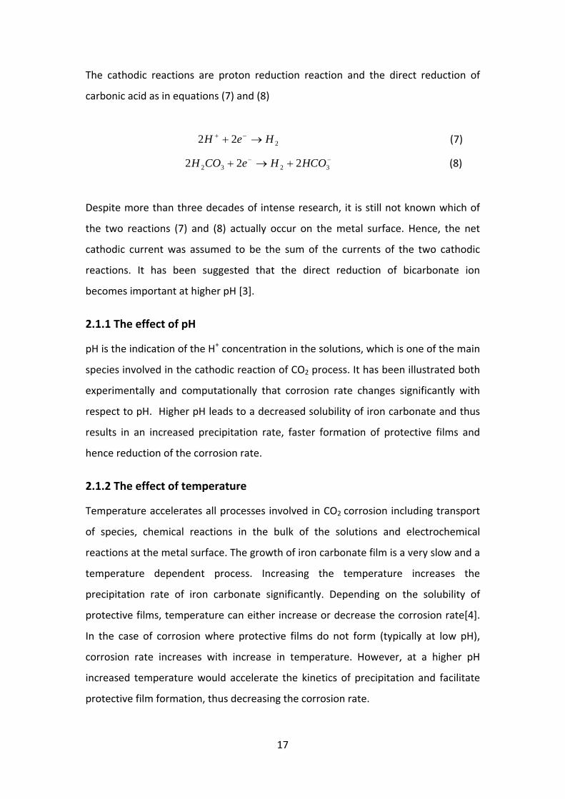
The cathodic reactions are proton reduction reaction and the direct reduction of

carbonic acid as in equations (7) and (8)

222 HeH (7)

3232 222 HCOHeCOH (8)

Despite more than three decades of intense research, it is still not known which of

the two reactions (7) and (8) actually occur on the metal surface. Hence, the net

cathodic current was assumed to be the sum of the currents of the two cathodic

reactions. It has been suggested that the direct reduction of bicarbonate ion

becomes important at higher pH [3].

2.1.1 The effect of pH

pH is the indication of the H+ concentration in the solutions, which is one of the main

species involved in the cathodic reaction of CO2 process. It has been illustrated both

experimentally and computationally that corrosion rate changes significantly with

respect to pH. Higher pH leads to a decreased solubility of iron carbonate and thus

results in an increased precipitation rate, faster formation of protective films and

hence reduction of the corrosion rate.

2.1.2 The effect of temperature

Temperature accelerates all processes involved in CO2 corrosion including transport

of species, chemical reactions in the bulk of the solutions and electrochemical

reactions at the metal surface. The growth of iron carbonate film is a very slow and a

temperature dependent process. Increasing the temperature increases the

precipitation rate of iron carbonate significantly. Depending on the solubility of

protective films, temperature can either increase or decrease the corrosion rate[4].

In the case of corrosion where protective films do not form (typically at low pH),

corrosion rate increases with increase in temperature. However, at a higher pH

increased temperature would accelerate the kinetics of precipitation and facilitate

protective film formation, thus decreasing the corrosion rate.

18

2.2. H2S Corrosion

The internal corrosion of carbon steel in the presence of hydrogen sulfide represents

a significant problem for both oil refineries and natural gas treatment facilities.

Surface scale formation is one of the important factors governing the corrosion rate.

The scale growth depends primarily on the kinetics of scale formation. In contrast to

relatively straight forward iron carbonate precipitation in pure CO2 corrosion, in an

H2S environment many types of iron sulfide may form such as amorphous ferrous

sulfide, mackinawite, cubic ferrous sulfide, smythite, greigte, pyrrhotite, troilite and

pyrite, among which mackinawite is considered to form first on the steel surface by a

direct surface reaction[5]. The poorly known mechanism of H2S corrosion makes it

difficult to quantify the kinetics of iron sulfide scale formation.

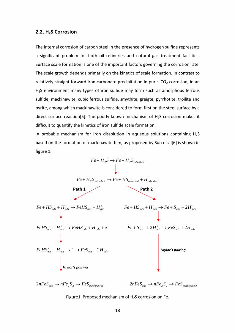
A probable mechanism for Iron dissolution in aqueous solutions containing H2S

based on the formation of mackinawite film, as proposed by Sun et al[6] is shown in

figure 1.

adsorbedSHFeSHFe 22

adsorbedadsorbedadsorbed HHSFeSHFe 2

Path 1 Path 2

adsadsadsads HFeHSHHSFe adsadsadsads HSFeHHSFe 2

eHFeHSHFeHS adsadsadsads adsadsadsads HFeSHSFe 22

adsadsadsads HFeSeHFeHS 2 Taylor’s pairing

Taylor’s pairing

emackinawitads FeSSnFenFeS 222 emackinawitads FeSSnFenFeS 222

Figure1. Proposed mechanism of H2S corrosion on Fe.

19

2.2.1. The effect of pH

The protective nature and composition of the corrosion product depend greatly on

the pH of the solution. At lower values of pH (<2), iron is dissolved and iron sulfide is

not precipitated on the surface of the metal due to a very high solubility of iron

sulfide phases at pH values less than 2. In this case, H2S exhibits only the accelerating

effect on the dissolution of iron. At pH values from 3 to 5, inhibitive effect of H2S is

seen due to the formation of ferrous sulfide (FeS) protective film on the electrode

surface [7].

2.2.2. The effect of H2S Concentration

H2S concentration has an immense influence on the protective ability of the sulfide

film formed. As the concentration of H2S increases, the film formed is rather loose

even at pH 3‐5 and does not contribute to the corrosion inhibiting effect[8].

2.2.3. The effect of temperature

The temperature dependence of H2S corrosion is very weak for short term exposure

and does not seems to have an effect at longer exposure times. This suggest that the

corrosion rate is predominantly controlled by the presence of iron sulfide scale[5].

2.3. CO2/H2S Corrosion

The internal corrosion of mild steel in the presence of both CO2 and H2S represents a

significant problem for oil and gas industries. Although the interaction of H2S with

low carbon steels have been published by various authors, the understanding of the

effect of H2S on CO2 corrosion is still limited because the nature of the interaction

with carbon steel is complicated.

In the presence of H2S, additional chemical reactions occurring in the bulk of the

solution include:

Dissociation of dissolved H2S is given in equation (9).

HSHSH SHK 22 (9)

where SH

HSHK SH

22

20

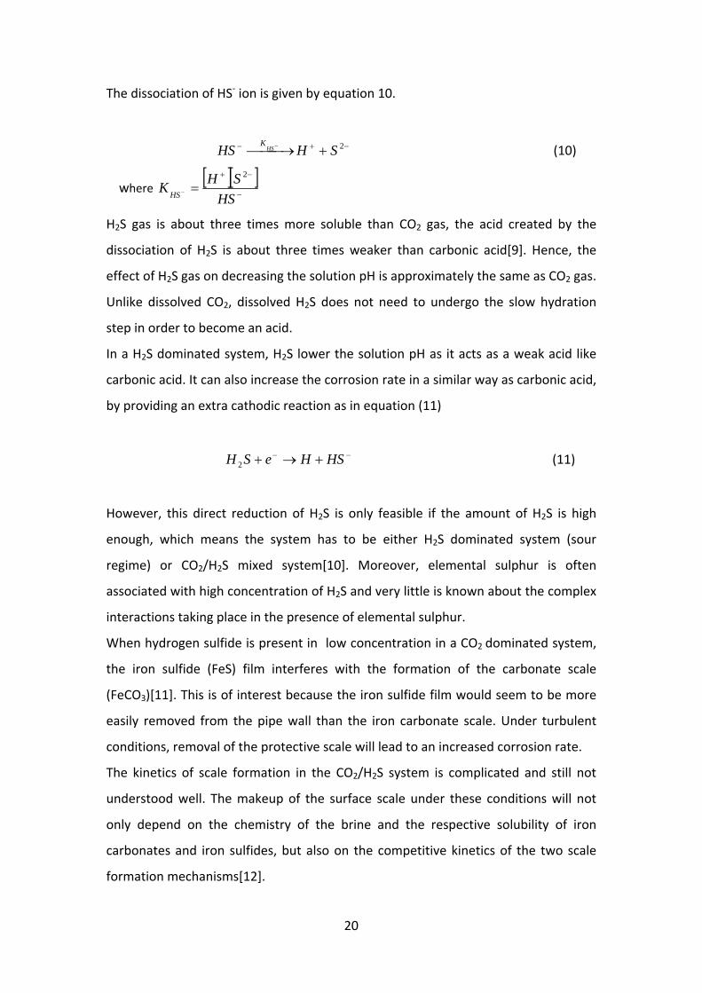
The dissociation of HS‐ ion is given by equation 10.

2SHHS HSK

(10)

where

HS

SHK

HS

2

H2S gas is about three times more soluble than CO2 gas, the acid created by the

dissociation of H2S is about three times weaker than carbonic acid[9]. Hence, the

effect of H2S gas on decreasing the solution pH is approximately the same as CO2 gas.

Unlike dissolved CO2, dissolved H2S does not need to undergo the slow hydration

step in order to become an acid.

In a H2S dominated system, H2S lower the solution pH as it acts as a weak acid like

carbonic acid. It can also increase the corrosion rate in a similar way as carbonic acid,

by providing an extra cathodic reaction as in equation (11)

HSHeSH 2 (11)

However, this direct reduction of H2S is only feasible if the amount of H2S is high

enough, which means the system has to be either H2S dominated system (sour

regime) or CO2/H2S mixed system[10]. Moreover, elemental sulphur is often

associated with high concentration of H2S and very little is known about the complex

interactions taking place in the presence of elemental sulphur.

When hydrogen sulfide is present in low concentration in a CO2 dominated system,

the iron sulfide (FeS) film interferes with the formation of the carbonate scale

(FeCO3)[11]. This is of interest because the iron sulfide film would seem to be more

easily removed from the pipe wall than the iron carbonate scale. Under turbulent

conditions, removal of the protective scale will lead to an increased corrosion rate.

The kinetics of scale formation in the CO2/H2S system is complicated and still not

understood well. The makeup of the surface scale under these conditions will not

only depend on the chemistry of the brine and the respective solubility of iron

carbonates and iron sulfides, but also on the competitive kinetics of the two scale

formation mechanisms[12].

21

2.4. Corrosion product film formation

CO2/H2S corrosion on the metal surface is strongly dependent on the type of

corrosion product film formed on the surface of the metal during the corrosion

process. The precipitation rate or the formation of these films depends on various

environmental factors and greatly on the concentration of species. The stability,

protectiveness, and adherence of these films determine the nature and the rate of

corrosion. Depending on the composition, the corrosion films can be of different

forms.

2.4.1. Iron carbide (Fe3C)

Iron carbide is an undispersed component of mild steel, which is left behind after

the corrosion of iron from the steel structure. Iron carbide films are conductive

electrically, very porous and non‐protective[13] films can significantly affect the

corrosion process by either decreasing the corrosion rate by acting as a diffusion

barrier, or increasing the corrosion by increasing the active specimen surface area by

forming a conductive bridge between the counter and working electrodes. Also, this

kind of film formation could result in galvanic coupling of the film to the metal or

acidification of the solution inside the corrosion product film which is very dangerous

and by far the strongest reason that could be given for the occurrence of localized

corrosion.

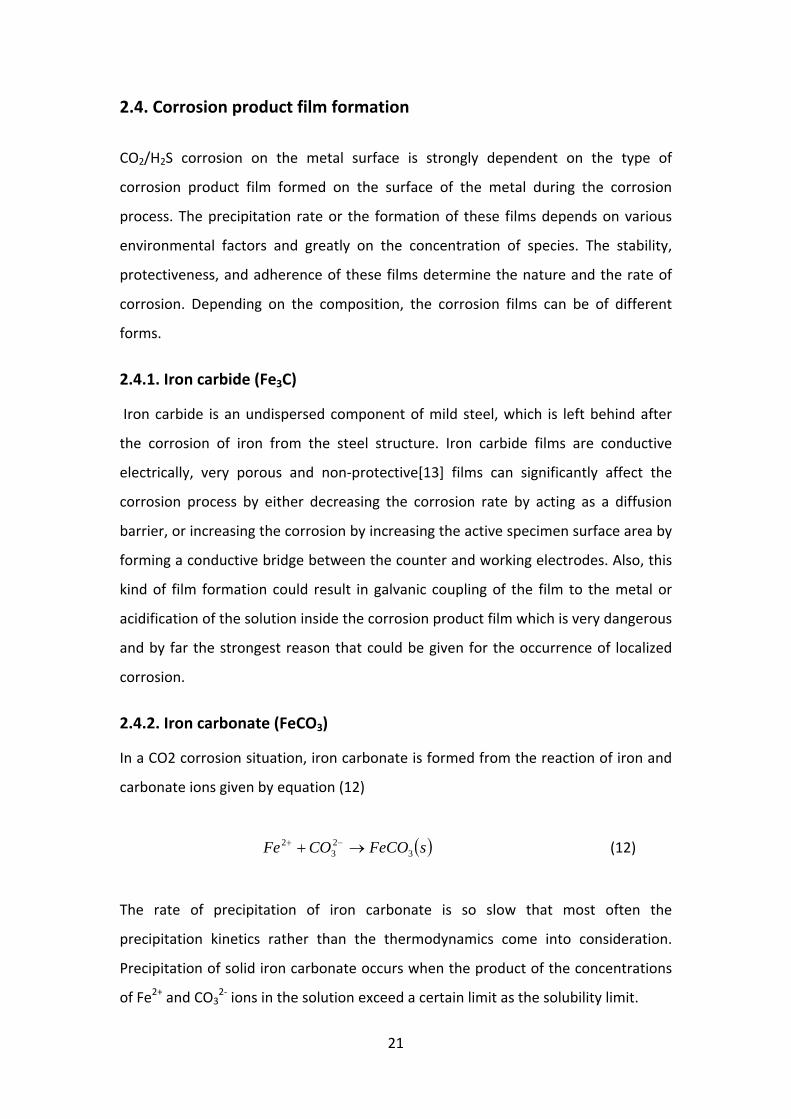
2.4.2. Iron carbonate (FeCO3)

In a CO2 corrosion situation, iron carbonate is formed from the reaction of iron and

carbonate ions given by equation (12)

sFeCOCOFe 323

2 (12)

The rate of precipitation of iron carbonate is so slow that most often the

precipitation kinetics rather than the thermodynamics come into consideration.

Precipitation of solid iron carbonate occurs when the product of the concentrations

of Fe2+ and CO32‐ ions in the solution exceed a certain limit as the solubility limit.

22

The rate of precipitation of the iron carbonate ( )()(3 sFeCOR can be expressed by the

equation (13) [2]

)()(33)(3 FeCOFeCOFeCO SfKspTf

V

AR

S (13)

where A/V is the surface area to volume ratio and KspFeCO3 is the solubility limit of

FeCO3.

The supersaturation S is defined as in equation (14)

3

23

2

3

FeCO

COFeFeCO Ksp

ccS

(14)

Since CO32‐ ion concentration is dependent on the pH, it can be deduced to eqn.15

),( 2 pHFefS (15)

Therefore, supersaturation and temperature are the most important factors

affecting the rate of precipitation, and the nature and protectiveness of the iron

carbonate film. Precipitation of iron carbonate on the surface of the metal decreases

the corrosion rate by acting as a diffusion barrier for the corrosive species to travel

to the metal surface by blocking few areas on the steel surface and preventing

electrochemical reactions from happening on the surface [14].

2.4.3. Iron sulfide (FeS) film

The structure and composition of the protective FeS film depends greatly on the

concentration of H2S in the system. The protective nature of the film mainly depends

on the pH of the solution [15]. At a solution pH value of 3 to 5, with a small

concentration of H2S, a protective film of FeS inhibits the corrosion rate of the metal

coupon[7]. In nearly neutral pH and at room temperature, mackinawite forms

through a solid state reaction, while at a pH value between 5 and 7, amorphous FeS

precipitates. The kinetics of FeS formation is complicated than the iron carbonate

film. The reaction for the formation of solid iron sulphide is given in equation (16).

)(22 sFeSSFe (16)

23

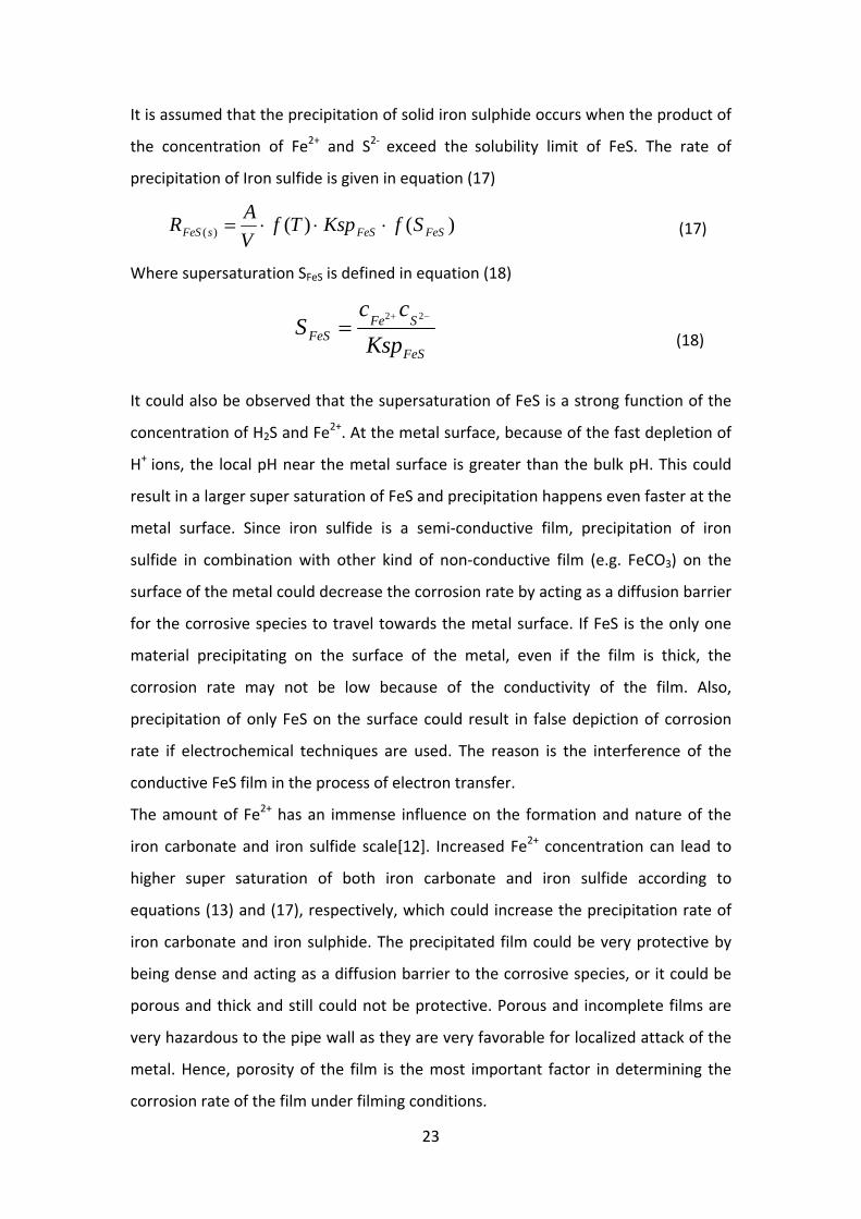
It is assumed that the precipitation of solid iron sulphide occurs when the product of

the concentration of Fe2+ and S2‐ exceed the solubility limit of FeS. The rate of

precipitation of Iron sulfide is given in equation (17)

)()()( FeSFeSsFeS SfKspTfV

AR (17)

Where supersaturation SFeS is defined in equation (18)

FeS

SFeFeS Ksp

ccS

22

(18)

It could also be observed that the supersaturation of FeS is a strong function of the

concentration of H2S and Fe2+. At the metal surface, because of the fast depletion of

H+ ions, the local pH near the metal surface is greater than the bulk pH. This could

result in a larger super saturation of FeS and precipitation happens even faster at the

metal surface. Since iron sulfide is a semi‐conductive film, precipitation of iron

sulfide in combination with other kind of non‐conductive film (e.g. FeCO3) on the

surface of the metal could decrease the corrosion rate by acting as a diffusion barrier

for the corrosive species to travel towards the metal surface. If FeS is the only one

material precipitating on the surface of the metal, even if the film is thick, the

corrosion rate may not be low because of the conductivity of the film. Also,

precipitation of only FeS on the surface could result in false depiction of corrosion

rate if electrochemical techniques are used. The reason is the interference of the

conductive FeS film in the process of electron transfer.

The amount of Fe2+ has an immense influence on the formation and nature of the

iron carbonate and iron sulfide scale[12]. Increased Fe2+ concentration can lead to

higher super saturation of both iron carbonate and iron sulfide according to

equations (13) and (17), respectively, which could increase the precipitation rate of

iron carbonate and iron sulphide. The precipitated film could be very protective by

being dense and acting as a diffusion barrier to the corrosive species, or it could be

porous and thick and still could not be protective. Porous and incomplete films are

very hazardous to the pipe wall as they are very favorable for localized attack of the

metal. Hence, porosity of the film is the most important factor in determining the

corrosion rate of the film under filming conditions.

24

Researchers[12] have found that the corrosion products formed in CO2/H2S system

depends on the competitiveness of iron carbonate and mackinawite. At high H2S

concentration and low Fe2+ concentration, mackinawite is the predominant scale

formed on the steel surface. At low H2S concentration and high Fe2+ concentration,

both iron carbonate and mackinawite are formed.

25

3. ELECTROCHEMICAL METHODS

3.1 Galvanic Corrosion

Galvanic corrosion, also referred to as two‐metal or bimetallic corrosion, occurs

when two dissimilar metals or alloys are in contact electrically while both are

immersed in an electrolyte solution. One of the two metals is corroded preferentially

by this type of corrosion; that is the most active or anodic metal corrodes rapidly

while the more noble or cathodic metal is not damaged. Galvanic attack can be

uniform in nature or localized at the junction between the alloys depending on

conditions. It can be particularly severe under the condition where protective

corrosion film does not form or where they are removed by condition of erosion

corrosion.

Every metal or alloy has a unique corrosion potential. Ecorr, when immersed in a

defined corrosive electrolytic solution. Thus, when two dissimilar metals are

connected in an aqueous environment, their differences in corrosion potentials will

cause corrosion. The metal with the more negative potential perform oxidation and

the other metal with more positive potential perform reduction. Thus, in a couple

between two metals A and B, the active metal A is the anode, while the noble metal

B is the cathode, with the corresponding reactions:

A → An+ + ne‐ (19)

Bm+ + me‐→ B (20)

Every metal has been rated for nobility and then placed on galvanic scales according

to nobility. Basically nobility is an indication of the resistance to corrosion, especially

of one metal contacting another metal. The relative nobility of a material can be

predicted by measuring its corrosion potential. The Galvanic series rank metals and

alloys in order of reactivity or electrical potential. Metals that are least noble are

very anodic, electropositive or high potential and will corrode most easily, whereas

metals that are more noble are highly cathodic, electronegative or low potential and

will be the more resistant to corrosion. The most corrosive effects will occur

between metals from the opposite ends of the galvanic scale or ranking of nobility.

26

Dissimilar metals in contact with each other in the presence of an electrolyte causes

current to flow through their points of contact at the expense of the metal with the

higher potential or less nobility. The much less noble metal is gradually consumed in

the electrochemical reaction and will deteriorate or wear away as the metal ions

migrate away from the very anodic metal to the more noble cathodic one. The more

noble metal's corrosion resistance actually increases from this transfer of ions to it

from the less noble metal, while the other metal is gradually getting consumed. Also,

oxides formed on a metal surface can form a galvanic couple with the same metal

with no oxide film as these two metal surface can have different potential [16].

A zero resistance ammeter (ZRA) is used to measure the galvanic coupling current

between two dissimilar electrodes. ZRA is a current to voltage converter that

produces a voltage output proportional to the current flowing between its two input

terminals while imposing a zero voltage drop to the external circuit.

3.2 Linear Polarization resistance

The Linear polarization resistance method, based on electrochemical concepts,

enables determination of instantaneous interfacial reaction rates such as corrosion

rates and exchange current densities from a single experiment.

Whenever the potential of an electrode is forced away from its value at open‐circuit,

that is referred to as polarizing the electrode. When an electrode is polarized, it can

cause current to flow through electrochemical reactions that occur at the electrode

surface. The amount of current is controlled by the kinetics of the reactions and the

diffusion of reactants both towards and away from the electrode.

In cells where an electrode undergoes uniform corrosion at open circuit, the open

circuit potential is controlled by the equilibrium between two different

electrochemical reactions. One of the reactions generates cathodic current and the

other anodic current.

27

Figure2. Linear Polarization Resistance Curve.

The open circuit potential ends up at the potential where the cathodic and the

anodic currents are equal. It is referred to as a mixed potential. The value of the

current for either of the reactions is known as the corrosion current. When there are

two simple, kinetically controlled reactions occurring, the potential of the cell is

related to the current by equation (21)

)()(303.2)(303.2

c

EocE

a

EocE

corr eeII

(21)

where,

I ‐ measured cell current in amps,

Icorr ‐ corrosion current in amps,

Eoc ‐ open circuit potential in volts,

βa ‐ anodic Beta coefficient in volts/decade

βc ‐ cathodic Beta coefficient in volts/decade.

If a small signal is applied in approximation to equation (21), equation (22) can be

obtained

)1

()(303.2 pca

cacorr R

I

(22)

28

Where, Rp ‐ polarization resistance

If the Tafel constants are known, Icorr can be calculated from Rp using equation (22).

Icorr in turn can be used to calculate the corrosion rate.

3.2.1 Calculation of corrosion rate from corrosion current

The corrosion current can be converted into corrosion rate by using Faraday’s law

nFMQ (23)

Where

Q‐ charge in coulombs

n‐ number of electrons transferred per molecule or atom

F ‐Faraday’s constant = 96487.7 coulombs/mole

M‐number of moles.

Equation (23) can be expressed in terms of equivalent weight (EW) by using the

relations EW= Atomic weight (AW)/n and M=W/AW. The expression for W, which is

the mass of the electro active species, is given in equation (24)

F

QEWW

(24)

Modifying equation (24) gives equation (25)

Ad

EWKICR corr

(25)

CR ‐ corrosion rate. Its units ate given by the choice of K

Icorr ‐ corrosion current in amperes

K ‐ constant =3272 mm/yr

EW ‐ equivalent weight in grams/equivalent

D ‐ density in grams /cm3

A ‐ sample area in cm2

This formula is valid only for uniform corrosion. In cases where localized corrosion

occurs, this cannot be used as it gives very low corrosion rate than actually is.

29

3.3 Potentiodynamic scan

Potentiodynamic polarization is a technique where the potential of the electrode is

varied at a selected rate by application of a current through the electrolyte. Through

the DC polarization technique, information on the corrosion rate, pitting

susceptibility, passivity, as well as the cathodic behavior of an electrochemical

system may be obtained.

In a potentiodynamic experiment, the driving force (i.e., the potential) for anodic or

cathodic reactions is controlled, and the net change in the reaction rate (i.e., current)

is observed. The potentiostat measures the current which must be applied to the

system in order to achieve the desired increase in driving force, known as the

applied current. As a result, at the open circuit potential the measured or applied

current will be zero.

3.3.1 The Anodic scan

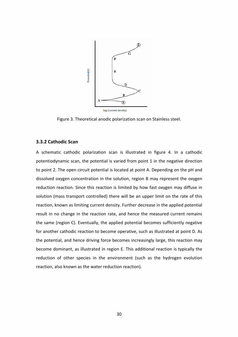
A schematic anodic polarization curve, typical for stainless steel is illustrated in figure

2. As shown in figure 2, the scan starts from point 1 and progresses in the positive

(potential) direction until termination at point 2. The open circuit potential is located

at point A. At this potential the sum of the anodic and cathodic reaction rates on the

electrode surface is zero. The region B is the active region, where metal oxidation is

the dominant reaction taking place. Point C is known as the passivation potential,

and as the applied potential increases above this value the current density is seen to

decrease with increasing potential (region D), until a low, passive current density is

achieved (passive region‐region E). Once the potential reached a sufficiently positive

value (point F, sometimes termed as breakaway potential) the applied current

rapidly increases (region G). This increase may be due to a number of phenomena,

depending on the alloy/environment combination. For some systems (e.g.,

aluminum alloys in salt water) this sudden increase in current may be pitting, while

for others it may be transpassive dissolution. For some alloys, typically those with a

very protective oxide, such as cobalt, the sudden increase in current is due to oxygen

evolution.

30

Figure 3. Theoretical anodic polarization scan on Stainless steel.

3.3.2 Cathodic Scan

A schematic cathodic polarization scan is illustrated in figure 4. In a cathodic

potentiodynamic scan, the potential is varied from point 1 in the negative direction

to point 2. The open circuit potential is located at point A. Depending on the pH and

dissolved oxygen concentration in the solution, region B may represent the oxygen

reduction reaction. Since this reaction is limited by how fast oxygen may diffuse in

solution (mass transport controlled) there will be an upper limit on the rate of this

reaction, known as limiting current density. Further decrease in the applied potential

result in no change in the reaction rate, and hence the measured current remains

the same (region C). Eventually, the applied potential becomes sufficiently negative

for another cathodic reaction to become operative, such as illustrated at point D. As

the potential, and hence driving force becomes increasingly large, this reaction may

become dominant, as illustrated in region E. This additional reaction is typically the

reduction of other species in the environment (such as the hydrogen evolution

reaction, also known as the water reduction reaction).

31

Figure 4. Theoretical cathodic polarization scan.

3.3.3 Corrosion rate from Potentiodynamic scan

For reactions which are essentially activation controlled, the current density can be

expressed as a function of the overpotential, η, which is expressed in equation (26)

0

logi

i (26)

Equation (26) is known as the Tafel equation, where β is the Tafel slope, i is the

applied current density, and i0 is the exchange current density.

Figure 5. Tafel slope calculation.

Thus, the Tafel slope for the anodic and cathodic reactions occurring at open circuit

may be obtained from the linear regions of the polarization curve, as illustrated in

32

figure 5. Once these slopes are established, it is possible to extrapolate back from

both the anodic and cathodic regions to the point where the anodic and cathodic

reaction rates (i.e., currents) are equivalent. The current density at that point is the

corrosion current density (icorr) and the potential at which it falls is the corrosion

potential (ECorr). The corrosion current density can then be used to calculate the

corrosion rate using equation (25).

3.4 Electrochemical Impedance Spectroscopy

Alternating Current (AC) impedance or Electrochemical Impedance Spectroscopy

(EIS) technique is one of the most powerful techniques for defining reaction

mechanisms, for investigating corrosion process and for exploring distributed

impedance system. Most generally, the application of the EIS technique has been

used by researchers for the evaluation of corrosion inhibitors, anodic coatings and

polymeric coatings. A brief introduction to the measurement technique is given

below:

The ability of a circuit element to resist the flow of electrical current is called

resistance. The resistance of an ideal resistor is defined by ohm’s law as the ratio

between the voltage E and current I as in equation (27)

I

ER (27)

An ideal resistor follows Ohm’s law at all voltage and current levels and its resistance

value is independent of frequency. Circuit elements which exhibit much more

complex behavior are encountered in real world situations where the simple concept

of ideal resistor cannot be applicable. Impedance is a more general circuit parameter

which is similar to resistance in a way that it is also a measure of the ability of the

circuit to resist the flow of electrical current but it is more complicated in its

behavior.

Electrochemical impedance is usually measured by applying an AC potential to an

electrochemical cell and measuring the current through the cell. When we apply a

33

sinusoidal potential excitation, the response to this potential is an AC current signal.

This current signal can be analyzed as a sum of sinusoidal functions.

Electrochemical impedance is normally measured using a small excitation signal. This

is done so that the cell’s response is pseudo‐linear. In a linear (or pseudo‐linear)

system, the current response to a sinusoidal potential will be a sinusoid at the same

frequency but shifted in phase.

The excitation signal, expressed as a function of time, has the form as equation (28)

)sin(0 tEEt (28)

Et is the potential at time t, E0 is the amplitude of the signal and ω is the radial

frequency. The relationship between radial frequency ω (expressed in

radians/second) and frequency f (expressed in hertz) is given by equation (29)

rf 2 (29)

In a linear system, the response signal, It is shifted in phase (φ) and has a different

amplitude, I0 as given in equation (30)

)sin(0 tII t (30)

An expression analogous to Ohm’s law can be used to calculate the impedance of

the system as in equation (31)

)sin(

)sin(

)sin(

)sin(0

0

0

t

tZ

tI

tE

I

EZ

t

t (31)

Using Euler’s relationship in equation (32)

sincos)exp( jj (32)

The impedance is then represented as a complex number as in equation (33)

)sin(cos)(exp()( 00 jZjZI

EZ (33)

Where I

EZ 0

The expression for impedance z is composed of both real and imaginary parts. A plot

of real part of impedance on X‐axis and negative of imaginary part of impedance on

Y‐axis is called Nyquist plot. Figure 6 shows the shape of Nyquist plot for the simple

equivalent circuit with one time constant, as shown in figure 7. The impedance on

the Nyquist plot can be represented as a vector of length |Z|. The angle between

this vector and the X‐axis is called the phase angle φ. The major short coming of a

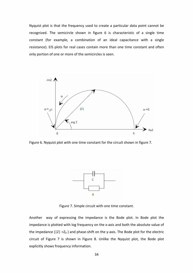
34

Nyquist plot is that the frequency used to create a particular data point cannot be

recognized. The semicircle shown in figure 6 is characteristic of a single time

constant (for example, a combination of an ideal capacitance with a single

resistance). EIS plots for real cases contain more than one time constant and often

only portion of one or more of the semicircles is seen.

Figure 6. Nyquist plot with one time constant for the circuit shown in figure 7.

Figure 7. Simple circuit with one time constant.

Another way of expressing the impedance is the Bode plot. In Bode plot the

impedance is plotted with log frequency on the x‐axis and both the absolute value of

the impedance (|Z| =Z0 ) and phase‐shift on the y‐axis. The Bode plot for the electric

circuit of Figure 7 is shown in Figure 8. Unlike the Nyquist plot, the Bode plot

explicitly shows frequency information.

35

Figure 8. Bode plot with one time constant.

3.4.1 Corrosion rate from impedance plot

In a Nyquist plot as shown in figure 9, at very high frequency, the imaginary

component, Z'' disappears, leaving only the solution resistance, Rs. At very low

frequency, Z'' again disappears, leaving a sum of Rs and the Faradaic reaction

resistance or polarisation resistance, Rp. The corrosion rate can be calculated by

using the Stern‐Geary equation by assuming a reasonable value for the beta

coefficients.

Low frequencyHigh frequency

Rs Rs+Rp10 260 510 760 10100

100

200

300

400

500

600

700

Z' (Ohm)

Z''

(Oh

m)

Figure 9. Nyquist plot showing the solution resistance and Polarization resistance.

36

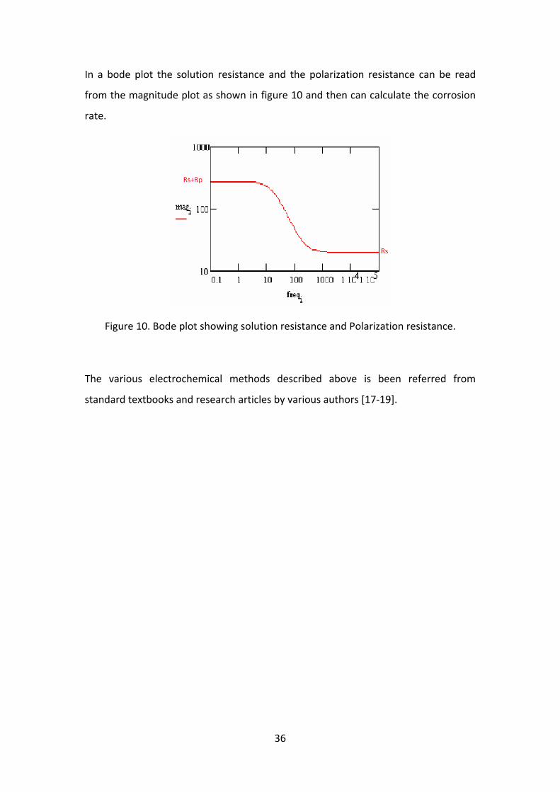
In a bode plot the solution resistance and the polarization resistance can be read

from the magnitude plot as shown in figure 10 and then can calculate the corrosion

rate.

Figure 10. Bode plot showing solution resistance and Polarization resistance.

The various electrochemical methods described above is been referred from

standard textbooks and research articles by various authors [17‐19].

37

4. EXPERIMENTAL PROCEDURE AND SETUP

Research objectives

The objective of this project is to study the corrosion behavior of carbon steel in the

presence of both CO2 and H2S in different pH and concentration. The test matrix for

the research is given in Table 1

Table1. The Experimental test matrix

Steel type St 52‐3

Standard electrolyte 0.5%NaCl

Temperature 22˚C (room temperature)

pH 3‐10

Concentration of sulfide 1mM ‐50mM

Pressure 1 bar

Carbon steel is used for this purpose because it is one of the most widely used metal

in the oil and gas industry. Table 2 shows the chemical composition of carbon steel

(St 52‐3), which was used for the research.

Table2. Chemical composition of Carbon Steel

Element Weight%

C 0.15

Si 0.30

Mn 1.20

P 0.019

S 0.01

Nb 0.002

Fe 98.319

The experiment was done in a galvanic setup with two carbon steel electrodes in

different electrolytic solution.

38

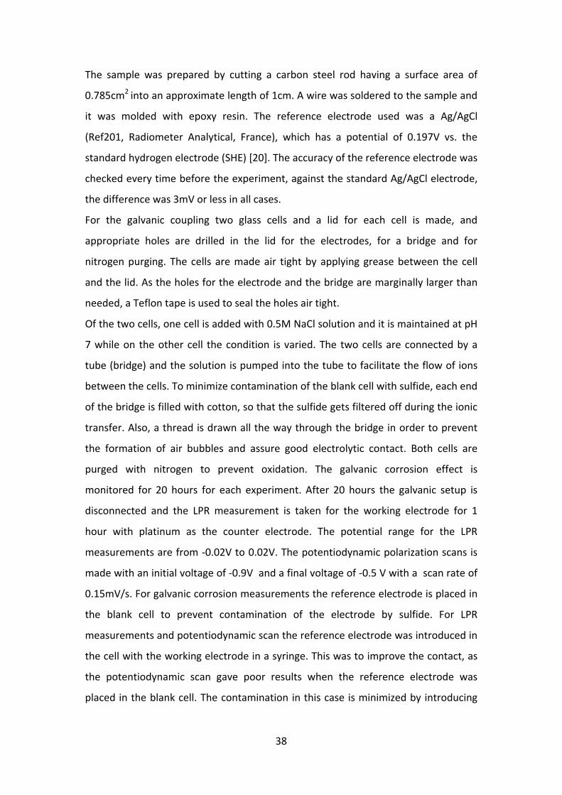
The sample was prepared by cutting a carbon steel rod having a surface area of

0.785cm2 into an approximate length of 1cm. A wire was soldered to the sample and

it was molded with epoxy resin. The reference electrode used was a Ag/AgCl

(Ref201, Radiometer Analytical, France), which has a potential of 0.197V vs. the

standard hydrogen electrode (SHE) [20]. The accuracy of the reference electrode was

checked every time before the experiment, against the standard Ag/AgCl electrode,

the difference was 3mV or less in all cases.

For the galvanic coupling two glass cells and a lid for each cell is made, and

appropriate holes are drilled in the lid for the electrodes, for a bridge and for

nitrogen purging. The cells are made air tight by applying grease between the cell

and the lid. As the holes for the electrode and the bridge are marginally larger than

needed, a Teflon tape is used to seal the holes air tight.

Of the two cells, one cell is added with 0.5M NaCl solution and it is maintained at pH

7 while on the other cell the condition is varied. The two cells are connected by a

tube (bridge) and the solution is pumped into the tube to facilitate the flow of ions

between the cells. To minimize contamination of the blank cell with sulfide, each end

of the bridge is filled with cotton, so that the sulfide gets filtered off during the ionic

transfer. Also, a thread is drawn all the way through the bridge in order to prevent

the formation of air bubbles and assure good electrolytic contact. Both cells are

purged with nitrogen to prevent oxidation. The galvanic corrosion effect is

monitored for 20 hours for each experiment. After 20 hours the galvanic setup is

disconnected and the LPR measurement is taken for the working electrode for 1

hour with platinum as the counter electrode. The potential range for the LPR

measurements are from ‐0.02V to 0.02V. The potentiodynamic polarization scans is

made with an initial voltage of ‐0.9V and a final voltage of ‐0.5 V with a scan rate of

0.15mV/s. For galvanic corrosion measurements the reference electrode is placed in

the blank cell to prevent contamination of the electrode by sulfide. For LPR

measurements and potentiodynamic scan the reference electrode was introduced in

the cell with the working electrode in a syringe. This was to improve the contact, as

the potentiodynamic scan gave poor results when the reference electrode was

placed in the blank cell. The contamination in this case is minimized by introducing

39

some cotton in the tube connected to the syringe. Figure 11 and 12 shows the

experimental setup in detail.

As the carbonate film formed under CO2 environment need longer time to form than

the sulfide film in H2S environment, the samples are stored in a container with saline

water purged with CO2. The samples are kept in this environment for 40days before

the start of the first experiment. The temperature of the environment was 20⁰C for

the first 20 days and the temperature was raised to 40⁰C for the next 20 days. The

raise in temperature is to increase the film formation rate, as higher temperature

enhances the rate of precipitation.

Figure 11. The Galvanic cell.

Figure 12. Diagram of the Galvanic cell‐ 1) 0.5M NaCl solution, 2) Counter electrode, 3) Reference electrode, 4) Bridge, 5) Working electrode, 6) Platinum electrode (for

LPR measurement and Tafel scans), 7) The experimental solution, 8)Syringe (to insert reference electrode during LPR and Tafel scans), 9) Rubber bulb.

40

The experiments were performed with sodium sulfide as the source for H2S gas, as

the use of H2S gas directly needs elaborate safety measures. Hence the amount of

H2S produced depends on the pH of the solution. All the experiments are done with

the Gamry Potentiostat. For galvanic measurement it was connected in zero

resistance ammeter (ZRA) mode, which means metal 1 is connected as working

electrode, metal 2 as the counter electrode and the reference to reference electrode

The electrodes are polished with P120 silicon carbide paper before the start of each

experiment. After each experiment an enlarged image of the working electrode is

taken. The SEM imaging was also done to study the surface characteristics of the

film. The SEM (Scanning Electron Microscope) EDX (Energy dispersive X‐ray) analysis

was done to find the elemental composition in the metal film. The accelerating

voltage applied for SEM imaging was 10kV, in order to get a clear surface structure

without damaging the surface film, as higher accelerating voltage gives high

resolution but unclear surface structure and can damage the film.

The electrochemical impedance spectroscopy (EIS) analysis was done for the

concentration of 10mM sulfide at pH 7 for a frequency range of 20,000 to 0.05Hz.

41

5. RESULTS AND DISCUSSION

The experimental results obtained are presented below based on the sulfide

concentration and pH.

Experimental Series 1:

a. H2S Corrosion‐ pH= 3, Concentration of Sulfide= 1mM, 10mM, 50mM

b. CO2/H2S Corrosion‐ pH= 3, Concentration of Sulfide= 1mM, 10mM, 50mM


a. H2S Corrosion‐ pH= 7, Concentration of Sulfide= 1mM, 10mM, 50mM

b. CO2/H2S Corrosion‐ pH= 7, Concentration of Sulfide= 1mM, 10mM, 50mM


a. H2S corrosion‐ pH= 10, Concentration of Sulfide= 1mM, 10mM, 50mM

b. CO2/H2S corrosion‐ pH= 10, Concentration of Sulfide= 1mM, 10mM, 50mM


a. H2S and CO2/H2S corrosion ‐EIS Analysis, Concentration of Sulfide= 10mM,

pH= 7

Experimental series 1a

The galvanic currents in experiments with various concentration of sulfide at pH 3

are shown in figure 13. The general corrosion rate was expected to be high at pH 3

and the presence of H2S is supposed to further increase the rate of corrosion. But,

the results obtained in the galvanic coupling shows negative current which means

that the working electrode (H2S environment) is more electronegative than the

counter electrode. This could be because of the film formation and hence the metal

getting passive. It was found that the open circuit potential (OCP) for the two surface

was different, a higher OCP at the working electrode (H2S environment) and a lower

OCP at the counter electrode (blank). In figure 13, it can be seen that for 30 minutes

to 1 hour the current was positive, suggesting that the passivation is due to film

formation. Figure 14 shows the galvanic potential, which is a mixed potential of the

working electrode and counter electrode, measured for 20 hours. It can be seen that

the potential gradually decreases to the more negative region, driving the anodic

current towards the counter electrode.

42

Work done by Han J et al [21] with iron carbonate film shows that in a galvanic

setup, under film forming condition the bare metal corrodes one or more orders of

magnitude faster than the film protected area. The result obtained was in

agreement with this research, showing a high level of protection of the working

electrode in a galvanic coupling but when the coupling is removed the metal shows

high degree of corrosion.

Figure 13. The change in galvanic current with time for concentration of sulfide at pH 3.

Figure 14. The galvanic potential versus time for various concentration of sulfide at pH 3.

43

Figure 15 shows the picture of the counter electrode taken after the end of the

experiment with 50mM sulfide concentration. It shows that a uniform corrosion has

occurred in the electrode. Figure 16 is the picture of the working electrode for the

same experiment. It can be seen that the surface is covered with a thick black film.

The corrosion rate of the two metal surfaces during the galvanic coupling was not

measured, but the result suggests that the film covered surface is protected by the

bare metal surface.

Figure 15 . Picture of the counter electrode for the experiment with a concentration of sulfide 50mM.

Figure 16. Picture of the working electrode for the experiment with a concentration of sulfide 50mM.

44

Figure 17 shows the potential measured with the various electrochemical

techniques. Ec(Rp) and Ec(Tafel) are measured only for the working electrode after

disconnecting the galvanic setup. At pH 3 as shown in figure 17 the galvanic potential

was lower than the potential measured with LPR and Tafel. When compared with the

potential‐pH diagram (the Pourbaix diagram) for iron in figure 46 and 47, this

potential is in the active region of corrosion.

Figure 17. The change in potential at different concentration of sulfide at pH 3.

Figure 18 shows the potentiodynamic sweeps for various concentration of sulfide. It

can be seen that at a higher concentration of sulfide (50mM) the corrosion current is

increasing suggesting that, higher the concentration of sulfide more will be rate of

corrosion. Figure 19 shows the corrosion rate calculated with LPR and Tafel. In

general, the corrosion rate, calculated with LPR shows higher value than the rate

measured with Tafel. But, the trend is the same for both types of measurement.

45

Figure 18. The potentiodynamic sweeps for various concentration of sulfide‐1mM, 10mM, 50mM at pH 3 with bubbling N2.

0

0.5

1

1.5

2

2.5

3

3.5

4

4.5

5

1mM 10mM 50mM

Concentration of sul fide

corr.rate (mm/yr)

LPR

Tafel

Figure 19. Effect of concentration on corrosion rate at pH 3 measured with LPR and Tafel.

Experimental series 1b

In this series, the experiments are done with the electrode pre‐corroded with CO2 for

various concentration of sulfide at pH 3. The result obtained in this series is also

similar to experimental series 1a. An important observation here is that the current

(figure 20) was negative from the beginning of the experiment for all concentration

of sulfides. This is because the electrode has an initial carbonate film when it was

exposed to sulfide, so the electrode gets immediate protection and the bare metal

starts corroding from the beginning. The potential (figure 21) measured with the

46

galvanic setup shows a gradual decrease in the potential, driving the corrosion

current in the opposite direction. Figure 22 shows the potential measured by all

three methods. It shows that the galvanic potential is lower than the potential

measured by LPR and Tafel. When compared with the Pourbaix diagram (figure 46

and 47) this potential without the galvanic coupling measured by LPR and Tafel are

well into the corrosion region.

Figure 20. The galvanic current versus time at pH 3 for various concentration of sulfide in the presence of CO2.

Figure 21. The galvanic potential versus time for various concentration of sulfide at pH 3 in the presence of CO2.

47

Figure 22. The change in potential at different concentration of

sulfide at pH 3 in the presence of CO2.

Figure 23. The potentiodynamic sweeps for various concentration of

sulfide‐ 1mM, 10mM, 50mM at pH 3 with N2 and CO2.

Figure 23 shows the potentiodynamic sweep of the working electrode at different

concentration of sulfide. It shows a gradual increase in corrosion current for increase

in the concentration of the sulfide. Figure 24 shows the corrosion rate calculated

with LPR and Tafel. The rate of corrosion in the presence of carbonate film is found

to be more than the one without carbonate film. Most of the literature[10] suggest

that the carbonate film forms a very strong protective layer and prevents corrosion.

But, the result of this experiment was not in agreement with this theory.

48

According to some recent research [21‐23], the passive carbonate film can be

depassivated by decrease in pH. Also, the carbon dioxide gas is not supplied

continuously into the experimental environment and this undersaturation could

have dissolved the iron carbonate film. As the film dissolves, the irregular surface

beneath the film provides more space for reaction and hence the corrosion rate is

very high.

0

0.5

1

1.5

2

2.5

3

3.5

4

4.5

5

1mM 10mM 50mM

Concentration of sulfide

corr.rate(m

m/yr)

LPR

Tafel

Figure 24. The effect of concentration on corrosion rate at pH 3 in the presence of CO2.


In this series of experiment the electrochemical measurements are taken at pH 7 for

various concentration of sulfide. In the galvanic coupling, both the metals are

immersed in solution with pH 7. The difference in environment is just by the sulfide

concentration. The galvanic measurement shows negative current (figure 25) which

means the counter electrode acts as anode. For at least 1 hour from the start of the

experiment the current remains positive and then turn negative, suggesting the

formation of film. The galvanic potential measurements (figure 26) show that the

decrease in potential is driving the current in the opposite direction.

49

Figure 25. The change in galvanic current with time for the concentration of sulfide‐1mM, 10mM, 50mM at pH 7.

Figure 26. The galvanic potential versus time for various concentration of sulfide at pH 7.

The potential measured for the working electrode without the galvanic coupling by

LPR and Tafel shows similar results as galvanic potential. In the pH range of 4 to 10,

the corrosion rate of iron is relatively independent of the pH of the environment

(figure 45). In this pH range the corrosion rate is governed largely by the rate at

which oxygen reacts with absorbed atomic hydrogen, thereby depolarizing the

50

surface and allowing the reduction reaction to continue. As the experiment was

done in presence of nitrogen the corrosion rate was very low for lower

concentration of sulfide. At neutral pH, sodium sulfide produces very little H2S,

depending on the concentration of the sulfide. Also Na2S form a metal precipitate

which is highly insoluble and prevents the metal from further attack. Thus, it can be

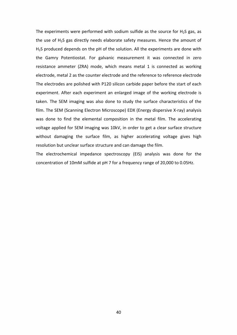
seen that the rate of corrosion (figure 29) is fairly high for 50mM sulfide

concentration (1.5 mm/yr) and for lower concentration the corrosion rate is

negligible. The potentiodynamic scan (figure 28) also shows that higher

concentration has higher degree of corrosion.

Figure 27. The change in potential at different concentration of sulfide at pH 7.

Figure 28. The potentiodynamic sweeps for various concentration of sulfide‐1mM, 10mM, 50mM at pH 7 with bubbling N2.

51

0

0.5

1

1.5

2

2.5

3

3.5

4

4.5

5

1mM 10mM 50mM


Corr.rate (mm/yr)

LPR

Tafel

Figure 29. Corrosion rate at various concentration of sulfide at pH 7 measured with LPR and Tafel.


In this series of experiment, the electrochemical measurement for the electrode

covered with iron carbonate film is done for various concentration of sulfide at pH7.

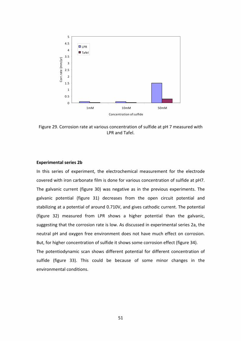
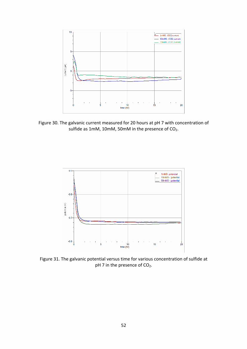
The galvanic current (figure 30) was negative as in the previous experiments. The

galvanic potential (figure 31) decreases from the open circuit potential and

stabilizing at a potential of around 0.710V, and gives cathodic current. The potential

(figure 32) measured from LPR shows a higher potential than the galvanic,

suggesting that the corrosion rate is low. As discussed in experimental series 2a, the

neutral pH and oxygen free environment does not have much effect on corrosion.

But, for higher concentration of sulfide it shows some corrosion effect (figure 34).

The potentiodynamic scan shows different potential for different concentration of

sulfide (figure 33). This could be because of some minor changes in the

environmental conditions.

52

Figure 30. The galvanic current measured for 20 hours at pH 7 with concentration of sulfide as 1mM, 10mM, 50mM in the presence of CO2.


53

Figure 32. The change in potential at different concentration of sulfide at pH 7 in the presence of CO2.

Figure 33. The potentiodynamic sweeps for various concentration of sulfide‐ 1mM, 10mM, 50mM at pH 7 with N2 and CO2.

54

0

0.5

1

1.5

2

2.5

3

3.5

4

4.5

5

1mM 10mM 50mM


corr.rate (mm/yr)

LPR

Tafel

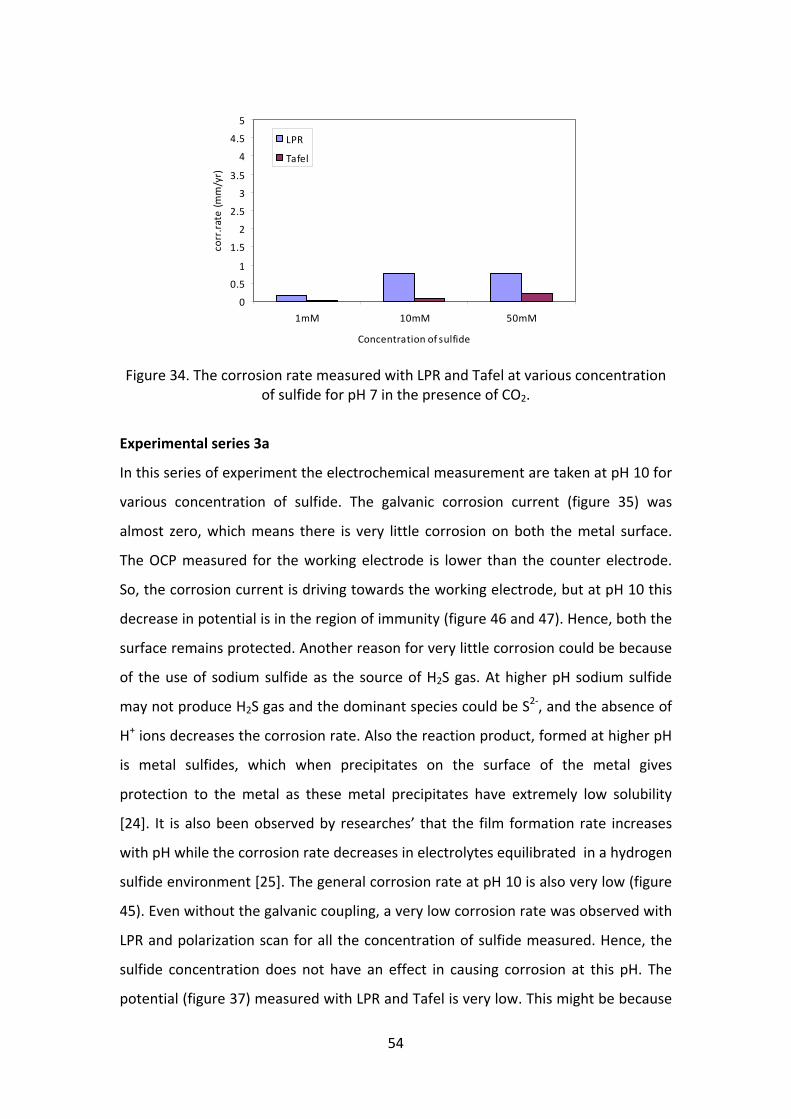
Figure 34. The corrosion rate measured with LPR and Tafel at various concentration of sulfide for pH 7 in the presence of CO2.


In this series of experiment the electrochemical measurement are taken at pH 10 for

various concentration of sulfide. The galvanic corrosion current (figure 35) was

almost zero, which means there is very little corrosion on both the metal surface.

The OCP measured for the working electrode is lower than the counter electrode.

So, the corrosion current is driving towards the working electrode, but at pH 10 this

decrease in potential is in the region of immunity (figure 46 and 47). Hence, both the

surface remains protected. Another reason for very little corrosion could be because

of the use of sodium sulfide as the source of H2S gas. At higher pH sodium sulfide

may not produce H2S gas and the dominant species could be S2‐, and the absence of

H+ ions decreases the corrosion rate. Also the reaction product, formed at higher pH

is metal sulfides, which when precipitates on the surface of the metal gives

protection to the metal as these metal precipitates have extremely low solubility

[24]. It is also been observed by researches’ that the film formation rate increases

with pH while the corrosion rate decreases in electrolytes equilibrated in a hydrogen

sulfide environment [25]. The general corrosion rate at pH 10 is also very low (figure

45). Even without the galvanic coupling, a very low corrosion rate was observed with

LPR and polarization scan for all the concentration of sulfide measured. Hence, the

sulfide concentration does not have an effect in causing corrosion at this pH. The

potential (figure 37) measured with LPR and Tafel is very low. This might be because

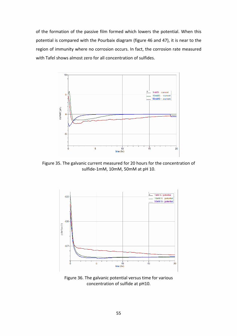
55

of the formation of the passive film formed which lowers the potential. When this

potential is compared with the Pourbaix diagram (figure 46 and 47), it is near to the

region of immunity where no corrosion occurs. In fact, the corrosion rate measured

with Tafel shows almost zero for all concentration of sulfides.

Figure 35. The galvanic current measured for 20 hours for the concentration of sulfide‐1mM, 10mM, 50mM at pH 10.

Figure 36. The galvanic potential versus time for various concentration of sulfide at pH10.

56

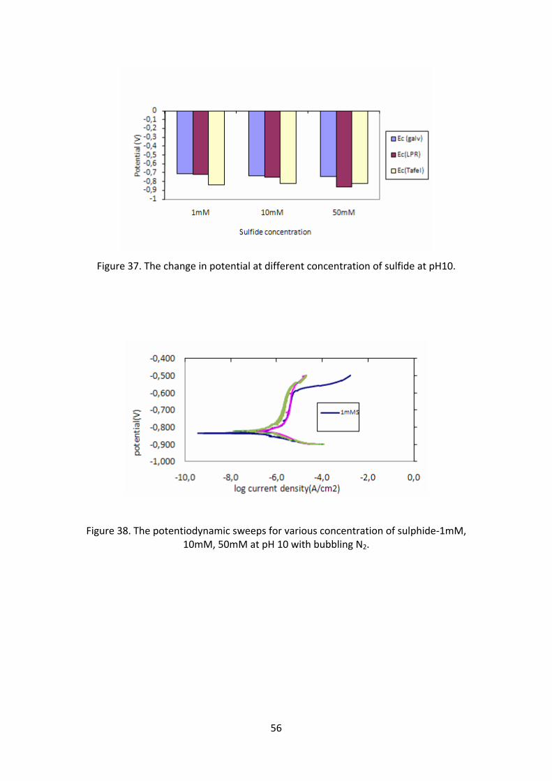
Figure 37. The change in potential at different concentration of sulfide at pH10.

Figure 38. The potentiodynamic sweeps for various concentration of sulphide‐1mM, 10mM, 50mM at pH 10 with bubbling N2.

57

Figure 39. The corrosion rate measured with LPR and Tafel at pH10 for various concentration of sulfide.


In this series of experiment the electrochemical measurements are taken for the

electrode pre‐corroded with CO2 at pH 10. The galvanic current (figure 40) here

shows positive, which means the working electrode (sulfide environment) is

corroding. As discussed in experimental series 3a, the sulfide and its reaction

product does not seem to increase the corrosion rate. But the results of galvanic

current shows mild corrosion effect on the working electrode, it could be because of

the difference in area between the two electrodes and also could be because of the

presence of carbonate film. The pre‐corroded metal surface has more area

compared to the bare metal surface because of the irregularity of the surface. In the

galvanic coupling the OCP measured for the working electrode was lower than the

counter electrode. But, at pH 10 this potential was in the region of immunity (figure

46 and 47). So, it can be assumed that the corrosion effect in the working electrode

could be because of the difference in area, which is making the working electrode as

anode. The potential (figure 42) measured from all three methods were very low,

suggesting that the probability of corrosion at this pH is negligible (from Pourbaix

diagram figure 46 and 47). The corrosion rate (figure 44) measured with LPR shows

around 1.5mm/yr for the concentration of 10mM sulfide and 50mM sulfide. This

corrosion rate may not be due to the concentration of sulfide because 10mM sulfide

shows slightly higher rate of corrosion than 50mM sulfide. This higher corrosion rate

58

than expected could be because of the irregular surface of the electrode. Also, the

reaction product of sodium sulfide may have interfered with the carbonate film and

might have caused a local condition near the metal surface, which enhances the

corrosion rate.

Figure 40. The galvanic current measured for 20 hours in the presence of CO2 for various concentration of sulfide.


59

Figure 42. The change in potential at pH 10 for various concentration of sulfide in the presence of CO2.

Figure 43. The potentiodynamic sweeps for various concentration of sulfide‐ 1mM, 10mM, 50mM at pH 10 with N2 and CO2.

60

0

0.5

1

1.5

2

2.5

3

3.5

4

4.5

5

1mM 10mM 50mMConcentration of sulfide

Corr.rate (mm/yr)

LPR

Tafel

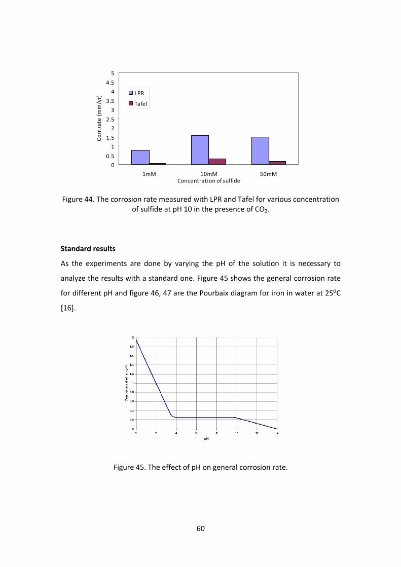
Figure 44. The corrosion rate measured with LPR and Tafel for various concentration of sulfide at pH 10 in the presence of CO2.

Standard results

As the experiments are done by varying the pH of the solution it is necessary to

analyze the results with a standard one. Figure 45 shows the general corrosion rate

for different pH and figure 46, 47 are the Pourbaix diagram for iron in water at 25⁰C

[16].

Figure 45. The effect of pH on general corrosion rate.

61

Figure 46. The potential‐pH diagram for Iron in water at 25⁰C

Figure 47. Theoretical conditions of corrosion, immunity and passivation of Iron.

Results of Blank

A set of experiment was done for pH 3, 7 and 10 without the addition of sulfide to

compare the experimental results. Figure 48 shows the corrosion rate measured

with Tafel and LPR. The LPR and the Tafel measurements for the working electrode

are taken after 20 hours of galvanic coupling with the neutral solution.

62

0.0

0.2

0.4

0.6

0.8

1.0

1.2

1.4

1.6

1.8

2.0

pH 3 pH 7 pH10

corr.rate(m

m/yr)

LPR

Tafel

Figure 48. Corrosion rate measured for blank with LPR and Tafel.

Experimental Series 4

EIS Analysis

The EIS analysis was done as part of learning this technique to measure the corrosion

rate. This technique was used to measure the corrosion rate for 10mM sulfide

concentration at pH 7 with and without the presence of CO2. The frequency range

used for this technique was 20,000Hz to 0.05Hz. The Nyquist plot for the

measurement with carbonate film is shown in figure 49. The measurement was

taken initially in the presence of only CO2 and N2 and then after adding sodium

sulfide. The lower frequency range is not small enough to determine exactly the

point where the line crosses the intercept. Hence, the line is extrapolated to

determine approximately the corrosion rate. The corrosion rate for the carbonate

film covered surface before adding sodium sulfide was about 3mm/yr (the β

coefficients was assumed to be 0.12V/decade for the corrosion rate calculation),

which is very high at this pH. This suggest that the film formed has dissolved in the

given environment and the irregular surface underneath was corroding at a higher

rate. From figure 49 it can be seen that the corrosion rate tends to decrease after

the addition of sodium sulfide. But as the data obtained was insufficient to calculate

exactly the corrosion rate it can be assumed to be around 1mm/yr. In the previous

experiments at pH 7, the corrosion rate was not measured during the start of the

experiment, but the rate calculated after 20 hrs (figure 34) was 0.8mm/yr.

63

0

10

20

30

40

50

60

70

8 18 28 38 48 58

Real(ohm)

-Im

ag(o

hm

)

CO2

After H2S

Figure 49. The Nyquist plot for CO2 and H2S corrosion.

Figure 50 shows the Nyquist plot for 10mM sulfide concentration in the presence of

nitrogen at pH7. Extrapolating the curve, the corrosion rate was calculated to be

0.86mm/yr, at the beginning of the experiment and this rate is reduced to about

0.54mm/yr after 20 hours. This suggests that the formation of the protective film is

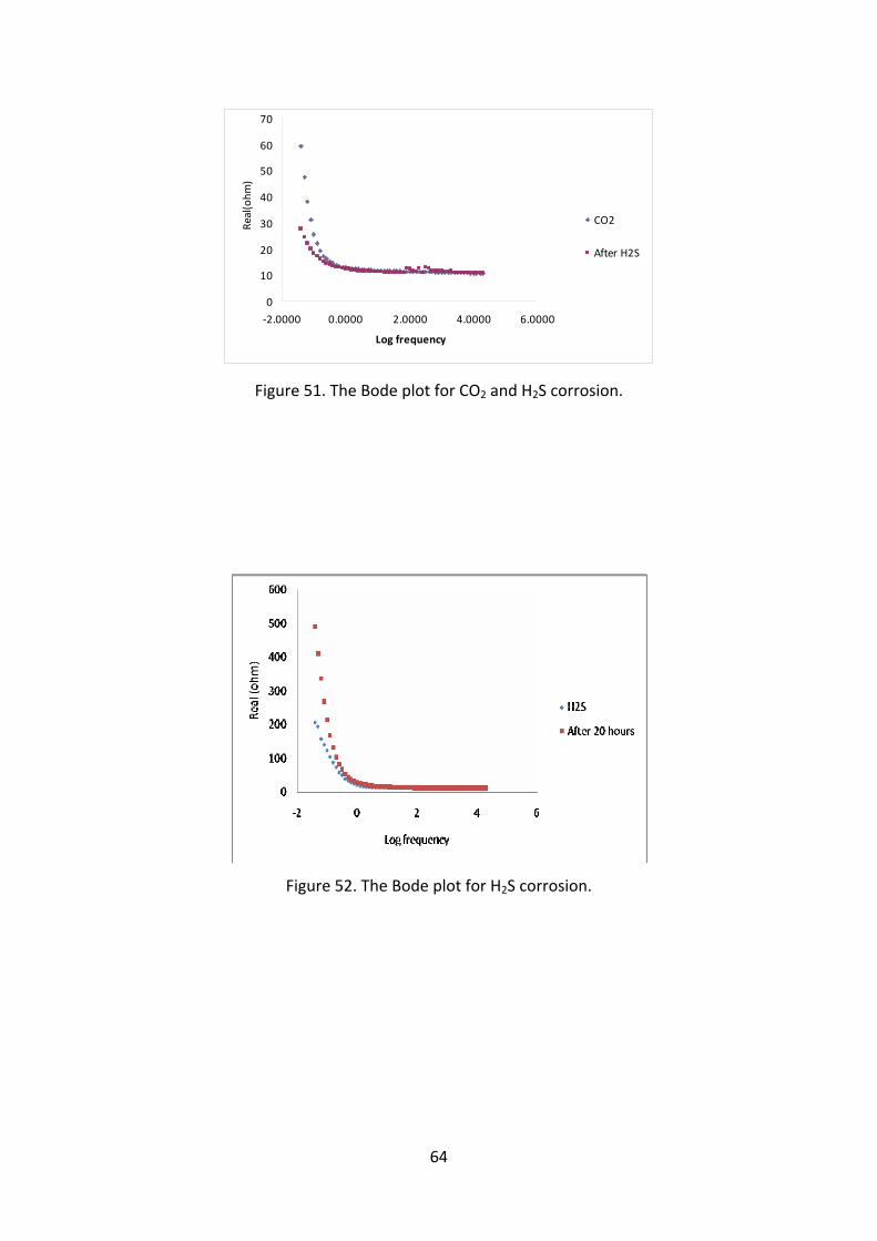
reducing the corrosion rate. Figure 51 and 52 shows the Bode plot for the same

experiment. As there is very little data available in the low frequency region it is not

possible to calculate the corrosion rate. Also, as the Bode plot cannot be

extrapolated to get a reasonably accurate result.

0

50

100

150

200

250

300

350

400

450

0 100 200 300 400 500 600Real (ohm)

-Im

ag (

oh

m)

H2S

After 20 hrs

Figure 50. The Nyquist plot for H2S corrosion.

64

0

10

20

30

40

50

60

70

‐2.0000 0.0000 2.0000 4.0000 6.0000

Log frequency

Real(ohm)

CO2

After H2S

Figure 51. The Bode plot for CO2 and H2S corrosion.

Figure 52. The Bode plot for H2S corrosion.

65

1mMS‐‐

1mMS‐‐

1mMS‐‐

1mMS‐‐/CO2

1mMS‐‐/CO2

1mMS‐‐/CO2

10mMS‐‐

10mMS‐‐

10mMS‐‐

10mMS‐‐/CO2

10mMS‐‐/CO2

10mMS‐‐/CO2

50mMS‐‐

50mMS‐‐

50mMS‐‐

50mMS‐‐/CO2

50mMS‐‐/CO2

50mMS‐‐/CO2

0 1 2 3 4 5

3

7

10

Corrosion rate (mm/yr)

Figure 53. Summary of corrosion rate measured with LPR.

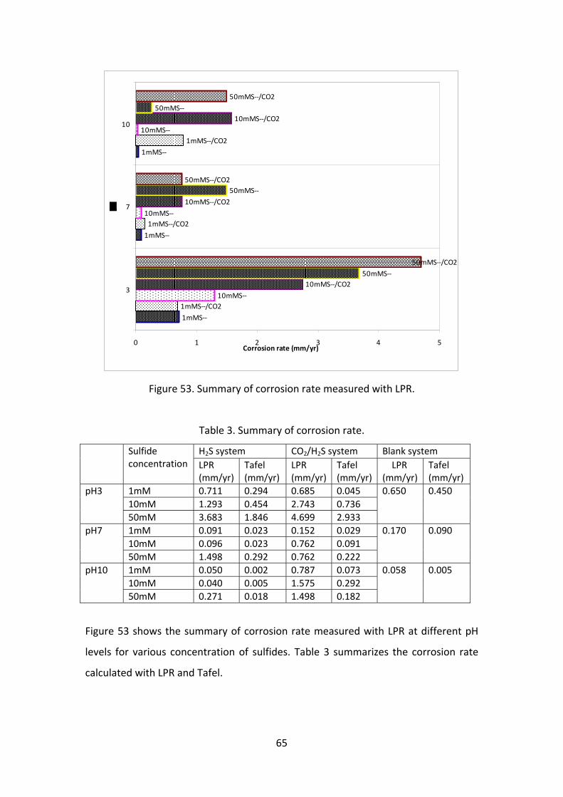
Table 3. Summary of corrosion rate.

H2S system CO2/H2S system Blank system Sulfide concentration LPR

(mm/yr)Tafel (mm/yr)

LPR (mm/yr)

Tafel (mm/yr)

LPR (mm/yr)

Tafel (mm/yr)

1mM 0.711 0.294 0.685 0.045

10mM 1.293 0.454 2.743 0.736

pH3

50mM 3.683 1.846 4.699 2.933

0.650 0.450

1mM 0.091 0.023 0.152 0.029

10mM 0.096 0.023 0.762 0.091

pH7

50mM 1.498 0.292 0.762 0.222

0.170 0.090

1mM 0.050 0.002 0.787 0.073

10mM 0.040 0.005 1.575 0.292

pH10

50mM 0.271 0.018 1.498 0.182

0.058 0.005

Figure 53 shows the summary of corrosion rate measured with LPR at different pH

levels for various concentration of sulfides. Table 3 summarizes the corrosion rate

calculated with LPR and Tafel.

66

In general, it was found that the corrosion rate is high in the CO2 /H2S system than it

is with just H2S. This could be because of the following reasons:

For CO2 /H2S corrosion the carbon dioxide gas is not supplied continuously in

the experimental environment. The experiment was done on pre‐corroded

electrode with CO2.

The passivation due to iron carbonate film was lost when the metal was

introduced in the H2S dominated system which has an undersaturation of

carbon dioxide

As the experiment was done on a pre‐corroded electrode there is more

surface available for H2S corrosion than the electrode which is not previously

corroded with CO2

The experiment was done for a short period of time. The long term exposure

could have given different result.

The H2S gas is not added directly, it is added in the form of sodium sulfide.

SEM Analysis

The SEM analysis was done to study the surface characteristics of the film. Figure 54

shows the SEM image of the carbonate film. At higher magnification the film shows

lots of cracks, which was not visible with naked eye. This crack is most probably

caused due to the drying of the sample while imaging in the SEM. Figure 55 shows

the SEM image of the film formed in the presence of both CO2 and H2S. The metal

chosen for this imaging is the working electrode of the experiment with 50mM

sulfide at pH 10. This electrode was chosen because the thickness of the film was

maximum at pH 10. The surface topography of figure 54 is different from that of

figure 55. The carbonate film (figure 54) is more rough or crystalline than the film

formed in the presence of sulfide. In figure 54, images (c) and (d) are of almost the

same magnification but the aperture size for (c) is 30 µm and for (d) is 60µm. The

aperture size is increased to see more clearly the surface characteristics, as smaller

aperture can give high depth of field but the resolution is not so good.

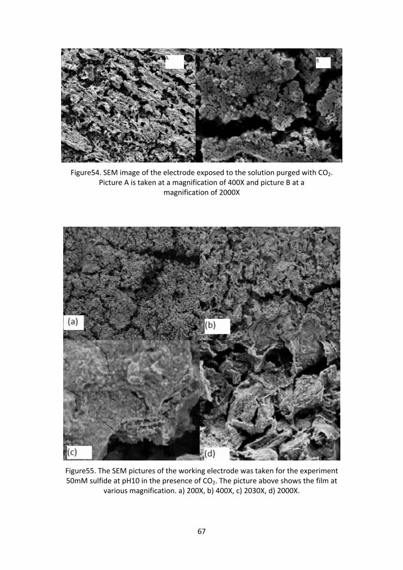
67

Figure54. SEM image of the electrode exposed to the solution purged with CO2. Picture A is taken at a magnification of 400X and picture B at a

magnification of 2000X

Figure55. The SEM pictures of the working electrode was taken for the experiment 50mM sulfide at pH10 in the presence of CO2. The picture above shows the film at

various magnification. a) 200X, b) 400X, c) 2030X, d) 2000X.

68

Figure 56 shows the cross section of the film at a magnification of 500X. The film

formed was thick and the thickness of the film was approximately 100µm. Figure 57

shows the EDX analysis of the film done nearer to the surface of the metal and at the

top of the film. It is found that at the surface of the film there was about 9% by

weight of sulfur and at the bottom of the film it was 7.7%. This suggests that the

carbonate film was more porous and the sulfide has penetrated through the film and

attacked the metal surface. But, this result cannot be considered as accurate as

sulfur is a low atomic weight species. The presence of silicon in the analysis is due to

the polishing of the sample with silicon carbide paper

Figure56. SEM image of the cross‐section of the film.

Figure57. The SEM X‐ray analysis of cross section of the film. The picture A is taken near the metal surface (bottom of the film) and picture B on top of the film.

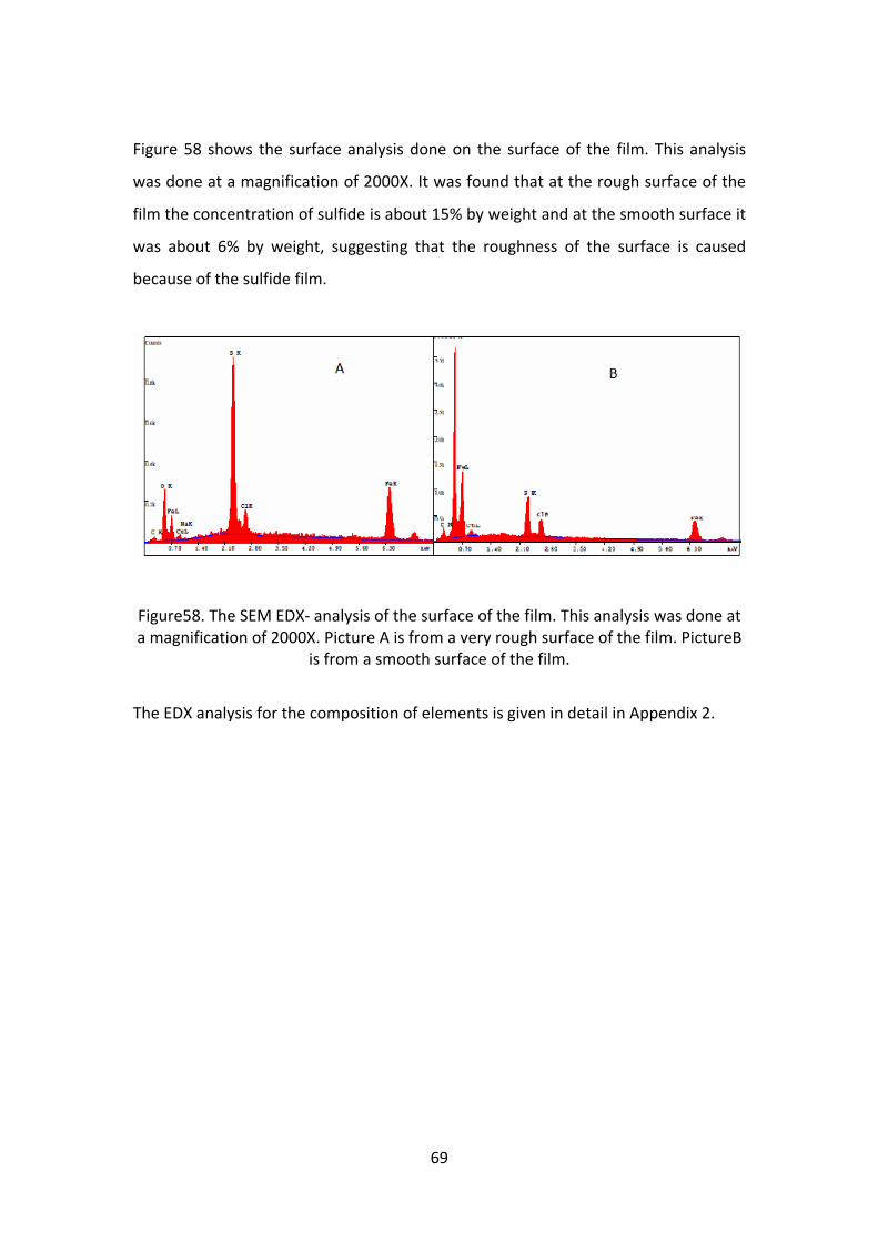
69

Figure 58 shows the surface analysis done on the surface of the film. This analysis

was done at a magnification of 2000X. It was found that at the rough surface of the

film the concentration of sulfide is about 15% by weight and at the smooth surface it

was about 6% by weight, suggesting that the roughness of the surface is caused

because of the sulfide film.

Figure58. The SEM EDX‐ analysis of the surface of the film. This analysis was done at a magnification of 2000X. Picture A is from a very rough surface of the film. PictureB

is from a smooth surface of the film.

The EDX analysis for the composition of elements is given in detail in Appendix 2.

70

6. CONCLUSION

From the experiments performed on carbon steel (St 52‐3) with galvanic coupling

and without the coupling, the following conclusions can be made:

In a galvanic coupling between metals, the metal exposed to even higher

concentration of sulfide and lower pH gets protected and the bare metal

which is in neutral pH was corroding.

The corrosion rate in general was high for lower pH levels and higher

concentration of sulfides.

The corrosion rate is higher for the CO2 /H2S system than in the presence of

only H2S.

The Iron carbonate film formed appears to be a loose film if the

concentration of the carbonate in the solution is not saturated. This

condition is more observed at lower pH.

71

7. RECOMMENDATIONS AND FUTURE WORK

As this thesis is a short term project, many aspects related to the topic had to be

overlooked because of the time limitation. The following could be some of the

recommendations for future work

Further study is needed on CO2 and H2S corrosion for higher temperature and

pressure, as the temperature and pressure are usually higher in oil and gas

pipelines.

All the experiments were done for a very limited period of 20‐24 hours. A

long term effect of the species on carbon steel can be investigated.

Further study can be done by supplying CO2 gas continuously into the

experimental environment.

72

8. REFERENCES

1. Zhao G.X, et al., 'Formation Characteristic of CO2 Corrosion Product layer of

P110 Steel Investigated by SEM and Electrochemical Technique'. Iron and

steel research International, Year 2009. 16( 4): p. 89‐94.

2. Hunnik E.W.J, V., Pots.B.F.M, and Hendriksen.E.L.J.A, The Formation of

Protective FeCO3 Corrosion Product Layers in CO2 Corrosion. Corrosion/96,

1996(Paper No.6).

3. Gray L.G.S, et al., Effect of pH and Temperature on the Mechanism of Carbon

Steel Corrosion by Aqueous Carbon Dioxide. Corrosion/90, 1990. Paper

No.40(Houston, TX: NACE International, 1990).

4. Nesic S. and Lee K.L.J, A Mechanistic Model of Iron Carbonate Film Growth

and the Effect on CO2 Corrosion of Mild Steel. Corrosion/02, 2002. Paper No.

237.

5. Sun W and Nesic S, A Mechanistic Model of H2S Corrosion of Mild Steel. NACE

Corrosion, 2007(Paper No.07655).

6. Sun W, Marquez A.I, and Botte G.G, Theoretical Investigation of H2S Corrosion

of Mild Steel. Institiute of Corrosion and Multiphase Technology.

7. Ma H.Y, et al., The influence of hydrogen sulfide on corrosion of iron under

different conditions. Corrosion Science, 1999(42): p. 1669‐1683.

8. Shoesmith D.W, et al., The Formation of Ferrous Monosulfide Polymorphs

during the Corrosion of Iron by Aqueous Hydrogen Sulfide at 210C.

Electrochemical Society, 1980. 127(5): p. 1007‐1015.

9. Rendon R.L and Alejandre J, Molecular Dynamics Simulations of the Solubility

of H2S and CO2 in Water. J.Mex.Chem.Soc2008. 52(1): p. 88‐92.

10. Hausler R.H and Godard H.P, Advances in CO2 Corrosion. NACE Publication,

1984. 1.

11. Srinivasan S and Kane R.D, Prediction of Corrosivity of CO2/H2S Production

Environment. Prevention of pipeline corrosion conference, Houston,TX, 1995.

12. Sun W and Nesic S, Kinetics of Iron Sulfide and Mixed Iron Sulfide/Carbonate

Scale Precipitation in CO2/H2S Corrosion. Corrosion NACExpo, 2006(Paper

No.06644).

13. Wang H.B, et al., Characterization of Inhibitor and Corrosion Product Film

using Electrochemical Impedance Spectroscopy(EIS). Corrosion 2001,

2001(Paper No.01023).

14. Nordsveen M, et al., A Mechanistic Model for Carbon Dioxide Corrosion of

Mild Steel in the Presence of Protective Iron Carbonate Films‐Part 1: Theory

and Verification. Corrosion Science, 2003. 59: p. 443‐456.

15. Ma H.Y, et al., Theoretical Interpretation on Impedance Spectra for Anodic

Iron Dissolution in Acidic Solutions Containing Hydrogen Sulfide. NACE

Corrosion 1998. 54(8).

73

16. Pourbaix M, Atlas of Electrochemical Equilibria in Aqueous Solutions. Nace

International., 1966.

17. Enos D.G and Scribner L.L, The Potentiodynamic Polarization Scan. Technical

Report 33, 1997.

18. Machiels A and Munson D, Predictive Model for Galvanic Corrosion. Electric

power research institute, 2004.

19. Lasia A, Electrochemical Impedance Spectroscopy and its Applications. Kluwer

Academic Publishers, 1999. 32: p. 143‐248.

20. Lundstrom M, Aromaa J, and Forsen O, Redox potential characteristics of

cupric chloride solutions. Science Direct‐ Hydrometallurgy, 2008. 95: p. 285‐

289.

21. Han J, et al., Roles of Passivation and Galvanic Effects in Localized CO2

Corrosion of Mild Steel. Corrosion 2008, NACE International, 2008. Paper No.

08332.

22. Han J, et al., Electrochemical Investigation of Localized CO2 Corrosion on Mild

Steel. corrosion 2007, NACE International, 2007(paper No.07323).

23. Sun W, Kinetics of Iron Carbonate and Iron Sulfide Scale Formation in CO2/H2S

Corrosion. PhD dissertation, 2006.

24. David R.B, Sodium Sulfides. Kirk‐Othmer Encyclopedia of Chemical

Technology, 1997.

25. Hemmingsen T, Hilbert L, and Nielsen L.V, Assessment of sulphur and H2S

corrosion by use of simultaneous ER, galvanic and optical measurements.

Eurocorr 2003.

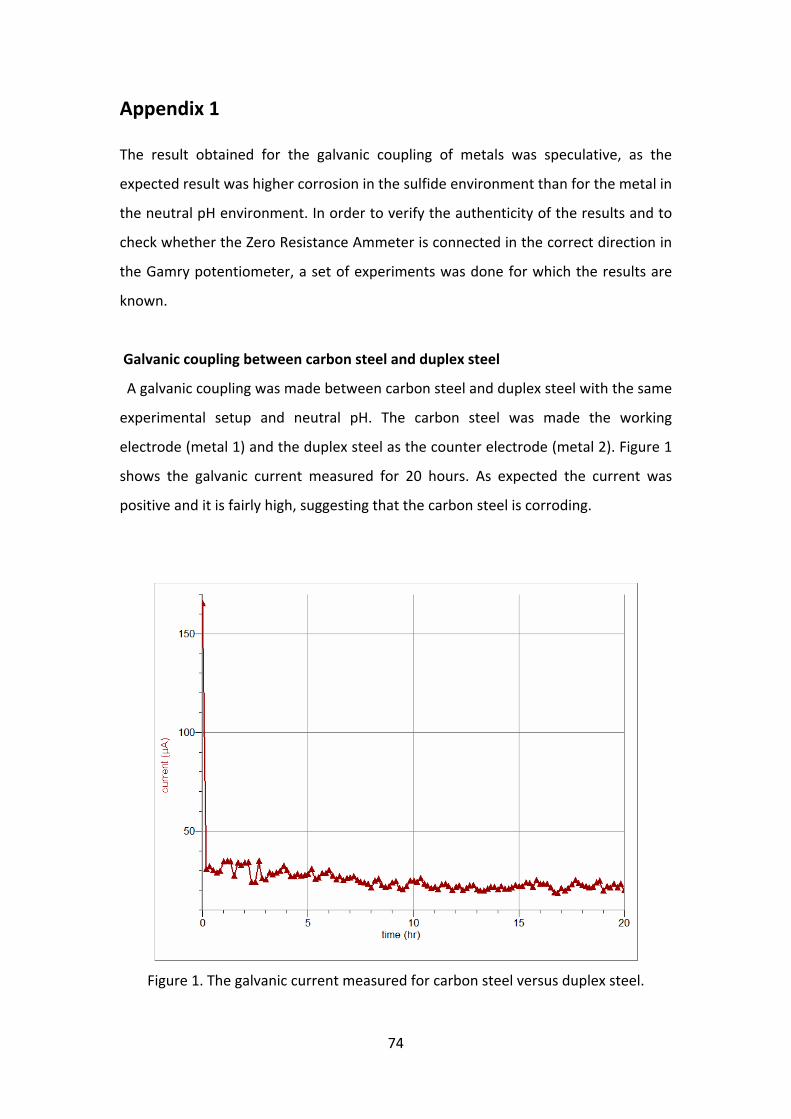
74

Appendix 1 The result obtained for the galvanic coupling of metals was speculative, as the

expected result was higher corrosion in the sulfide environment than for the metal in

the neutral pH environment. In order to verify the authenticity of the results and to

check whether the Zero Resistance Ammeter is connected in the correct direction in

the Gamry potentiometer, a set of experiments was done for which the results are

known.

Galvanic coupling between carbon steel and duplex steel

A galvanic coupling was made between carbon steel and duplex steel with the same

experimental setup and neutral pH. The carbon steel was made the working

electrode (metal 1) and the duplex steel as the counter electrode (metal 2). Figure 1

shows the galvanic current measured for 20 hours. As expected the current was

positive and it is fairly high, suggesting that the carbon steel is corroding.

Figure 1. The galvanic current measured for carbon steel versus duplex steel.

75

Figure 2 shows the galvanic potential measured for 20 hours between carbon steel

and duplex steel. The open circuit potential measured for carbon steel is lower than

the duplex steel and hence the carbon steel acts as anode and the duplex steel as

cathode. The potential measured is fairly constant for 20 hours.

Figure 2. The galvanic potential measured for carbon steel vs. duplex steel.

76

Appendix 2

The SEM‐ EDX Analysis

The SEM‐ EDX analysis is done to study the surface characteristics of the film. Figure

3 and 4 give a clear picture of the elemental composition of the cross section of the

film.

Figure 3. The SEM‐ EDX analysis of the cross‐section of the film. This analysis is done at the bottom of the film i.e., near the metal surface.

77

Figure 4. The SEM‐ EDX analysis of the cross‐section of the film. This analysis is done at the top of the film surface.

Figure 5 and 6 shows the SEM‐EDX analysis of the surface of the film. Figure 5 shows

the elemental composition at a rough surface of the film and figure 6 near the

smooth surface.

78

Figure 5. The SEM‐EDX analysis of the surface of the film. This analysis is done on the rough surface of the film, when the image magnification is 2000X.

79

Figure 6. The SEM‐EDX analysis of the surface of the film. This analysis was done on a smooth surface of the film when the image magnification was 2000X.

co2 and h2s corrosion in oil pipelines

Documents