University of Wollongong University of Wollongong

Research Online Research Online

University of Wollongong Thesis Collection 1954-2016 University of Wollongong Thesis Collections

2016

Modelling of CO2 release from high pressure pipelines Modelling of CO2 release from high pressure pipelines

Bin Liu University of Wollongong

Follow this and additional works at: https://ro.uow.edu.au/theses

University of Wollongong University of Wollongong

Copyright Warning Copyright Warning

You may print or download ONE copy of this document for the purpose of your own research or study. The University

does not authorise you to copy, communicate or otherwise make available electronically to any other person any

copyright material contained on this site.

You are reminded of the following: This work is copyright. Apart from any use permitted under the Copyright Act

1968, no part of this work may be reproduced by any process, nor may any other exclusive right be exercised,

without the permission of the author. Copyright owners are entitled to take legal action against persons who infringe

their copyright. A reproduction of material that is protected by copyright may be a copyright infringement. A court

may impose penalties and award damages in relation to offences and infringements relating to copyright material.

Higher penalties may apply, and higher damages may be awarded, for offences and infringements involving the

conversion of material into digital or electronic form.

Unless otherwise indicated, the views expressed in this thesis are those of the author and do not necessarily Unless otherwise indicated, the views expressed in this thesis are those of the author and do not necessarily

represent the views of the University of Wollongong. represent the views of the University of Wollongong.

Recommended Citation Recommended Citation Liu, Bin, Modelling of CO2 release from high pressure pipelines, Doctor of Philosophy thesis, School of Mechanical, Materials and Mechatronic Engineering, University of Wollongong, 2016. https://ro.uow.edu.au/theses/4950

Research Online is the open access institutional repository for the University of Wollongong. For further information contact the UOW Library: research-pubs@uow.edu.au

I

Modelling of CO2 release from high pressure pipelines

A thesis submitted in partial fulfilment of the requirements

for the award of the degree of

Doctor of Philosophy

by

Bin Liu

from Faculty of Engineering and Information Sciences, University of

Wollongong

August 2016

Wollongong, New South Wales, Australia

II

Thesis Certification

I, Bin Liu, declare that this thesis, submitted in fulfilment of the requirements for the award

of Doctor of Philosophy, at the School of Mechanical, Materials and Mechatronic

Engineering, University of Wollongong, is wholly my own work unless otherwise referenced

or acknowledged. The document has not been submitted for qualification at any other

academic institution.

Bin Liu

Feb. 2017

III

ABSTRACT

Carbon Capture and Storage (CCS) is widely seen as an effective technique to reduce what

are perceived to be excessive concentrations of Carbon Dioxide (CO2) in the atmosphere. In

the CCS chain, transportation of CO2 through high-pressure pipelines constitutes an

important link. Although CO2 pipelines are generally very safe, an unplanned release of CO2

from a pipeline presents a potential risk to human and animal populations as well as the

environment. Therefore, to facilitate the risk assessment, it is necessary to gain a better

understanding of CO2 releases from high-pressure pipelines, including the prediction of

depressurisation of the pipe flow, the near-field atmospheric expansion and the far-field

atmospheric dispersion.

An accurate prediction of CO2 depressurisation following pipeline fracture is crucial for the

design and operation for CCS, which requires the consideration of a number of complex and

interacting phenomena, such as the sharp drop of pressure and temperature, and the delayed

nucleation or delayed bubble formation. Usually, this analysis consists of a one-dimensional

decompression model that describes the conservation of mass, momentum and energy. The

fluid is usually considered to remain in thermal and mechanical equilibrium during the

depressurisation process, while the non-equilibrium liquid/vapour transition phenomena are

ignored. Although efforts have been made to model non-equilibrium two-phase CO2

depressurisation in recent years, possible improvement can be made by using a more precise

Equation of State (EOS) and more detailed models. Moreover, artificial CO2 tend to contain

some impurities, which can modify the behaviour of depressurisation significantly due to the

dramatic change in properties. However, there seems to be no comprehensive model coupling

with non-equilibrium phenomena, precise EOS and impurities in open publication to date. In

this thesis, a multi-phase CO2 pipeline decompression model using Computational Fluid

IV

Dynamics (CFD) techniques is presented. The GERG-2008 EOS is employed to describe the

properties of vapour and liquid phases. A phase change model using a mass transfer

coefficient to control the inter-phase mass transfer rate is implemented into the CFD code. By

varying the mass transfer coefficient, the effect of non-equilibrium phenomena (delayed

nucleation) on the decompression wave speed can be investigated. The proposed multi-phase

CFD decompression model is validated against the experimental data from ‘shock tube’ tests.

The performance of the proposed model is also compared with that of the ‘Homogeneous

Equilibrium Model’ (HEM). In addition, the influence of delayed nucleation on CO2 and CO2

mixture decompression characteristics is discussed and the optimum mass transfer

coefficients for pure CO2 and CO2 mixture are obtained. Also, the influence of the impurities

on the depressurisation process is investigated in this study. The results show that the non-

equilibrium phenomenon has a great effect on both CO2 and CO2 mixture pipe flow.

Moreover, the atmospheric expansion is investigated in this study to provide the boundary

conditions for the dispersion simulation. Two methods are involved. One is the CFD method,

which could provide more details. The other is an analytical model, which could avoid

resolving the high pressure gradients as well as possible dry ice formation.

In addition, the heavy gas dispersion model is proposed using the CFD method. Several CO2

dispersion experiments are simulated to validate the CFD model. Dispersion with two typical

release directions is investigated. One is vertical release and the other hypothetical release

direction is horizontal. The latter is considered as the worst case scenario. In the study of

vertical release, hypothetical release rates are used. CFD models for CO2 dispersion over

complex terrains are proposed. Four representative terrain types (a flat terrain with one hill, a

flat terrain with two hills, as urban area and a real terrain in Australia) are employed to

investigate terrain effects on dispersion behaviour. The results indicate that terrain features,

V

combined with the weather conditions, have significant influences on the pattern of CO2

dispersion. In the study of horizontal release, the release rate was obtained from the

depressurisation model. The results show that, for horizontal pipe releases, the consequence

distances are affected by the non-equilibrium effect during phase change in the pipeline.

However, the influence of wind speed and stagnation pressure on the consequence distance is

not so significant. Increase in wind speed or stagnation pressure leads to a longer

consequence distance for horizontal release. In contrast, the effects of pipe diameters on the

consequence distance are considerable.

VI

ACKNOWLEDEGMENTS

I would like to express my gratitude to all the people who give me support and help during

my research life. I appreciate my supervisors – Associate Professor Cheng Lu and Professor

Anh Kiet Tieu for their support, advice and guidance. My sincere and special thanks go to Dr.

Xiong Liu for his considerable support and valuable advice during the simulation work, as

well as his suggestions during the research and in revising the manuscript. Also, I would like

to thank other members and staffs in Energy Pipeline Cooperative Research Centre (EPCRC),

Australia, who have made this thesis possible.

This work was carried out at the School of Mechanical, Material and Mechatronics

Engineering, Faculty of Engineering, University of Wollongong. I would like to thank all my

colleagues and fellow PhD students for their precious advice and help during the research.

The funding and in-kind support from the EPCRC is gratefully acknowledged. Sincere thanks

to Scholarship from China Scholarship Council (CSC) and the University of Wollongong.

Also, I appreciate my supervisor Cheng Lu for his grant for my living costs during the study.

Finally, my deepest regards to my family members. Without their support and love I could

not have completed this research. I dedicate this thesis to them.

VII

TABLE OF CONTENTS

Thesis Certification ................................................................................................................... II

ABSTRACT ............................................................................................................................. III

ACKNOWLEDEGMENTS ..................................................................................................... VI

TABLE OF CONTENTS ....................................................................................................... VII

List of Figures ........................................................................................................................... X

List of Tables ........................................................................................................................ XIV

Nomenclature ......................................................................................................................... XV

Publications ........................................................................................................................ XVIII

Chapter 1 Introduction ............................................................................................................... 1

1.1 Background ..................................................................................................................... 1

1.2 Research objectives and activities ................................................................................. 7

Chapter 2 Literature review ..................................................................................................... 13

2.1 Equation of State .......................................................................................................... 15

2.1.1 RK EOS .................................................................................................................... 17

2.1.2 Peng-Robinson EOS ................................................................................................ 19

2.1.3 Span & Wagner EOS ............................................................................................... 20

2.1.4 GERG EOSs ............................................................................................................. 20

2.1.5 Composite EOS ........................................................................................................ 21

2.1.6 Comparison of EOSs ............................................................................................... 22

2.2 CO2 Pipeline decompression ....................................................................................... 23

2.2.1 Shock tube tests ........................................................................................................ 23

2.2.2 Decompression models ............................................................................................ 25

2.3 Source strength prediction models ............................................................................. 31

2.3.1 Equation for the choked exit condition .................................................................... 32

2.3.2 Wilson’s method [84] .............................................................................................. 33

2.3.3 Morrow model [85] ................................................................................................. 34

2.3.4 Phast modules .......................................................................................................... 35

2.3.5 EPCRC model .......................................................................................................... 38

2.4 Expansion to atmospheric pressure ............................................................................ 40

2.5 Phase change models .................................................................................................... 43

2.5.1 The process of phase change during the release and dispersion ............................ 43

2.5.2 Phase change models based on temperature relaxation ......................................... 45

VIII

2.5.3 The phase change models based on energy ............................................................. 47

2.5.4 Phase change models based on pressure relaxation involving with CO2 ............... 49

2.6 Dispersion models ......................................................................................................... 51

2.6.1 “Gassian-based” models ......................................................................................... 51

2.6.2 “Similarity-profile” models ..................................................................................... 52

2.6.3 CFD dispersion model ............................................................................................. 59

2.7 Knowledge gaps ............................................................................................................ 66

2.8 Summary ....................................................................................................................... 66

Chapter 3 Multi-phase decompression modelling of pure CO2 considering non-equilibrium phase transfer ........................................................................................................................... 68

3.1 Introduction .................................................................................................................... 69

3.2 Methodology ................................................................................................................. 72

3.2.1 Computational domain ............................................................................................ 72

3.2.2 The mixture multi-phase model ............................................................................... 73

3.2.3 Numerical Methods.................................................................................................. 75

3.2.4 Thermodynamic property modelling ...................................................................... 76

3.2.5 Source terms ............................................................................................................ 77

3.3 Results and discussion .................................................................................................. 79

3.4 Summary ..................................................................................................................... 101

Chapter 4 Multi-phase decompression modelling of CO2 mixture considering non-equilibrium phase transfer ...................................................................................................... 103

4.1 Introduction ................................................................................................................ 104

4.2 Methodology ............................................................................................................... 105

4.3 Results and discussion ................................................................................................ 107

4.4 Summary ..................................................................................................................... 119

Chapter 5 CFD simulation of under-expanded CO2 jet ......................................................... 121

5.1 Introduction ................................................................................................................ 122

5.2 Simulation model ........................................................................................................ 123

5.3 Air jet using user-defined real gas model ................................................................ 123

5.4 CO2 jet using PR EOS ................................................................................................ 129

5.5 Summary ..................................................................................................................... 133

Chapter 6 CFD simulation of CO2 dispersion in a complex environment ............................. 135

6.1 Introduction ................................................................................................................ 136

6.2 Numerical methods .................................................................................................... 139

IX

6.3 Experimental validation ............................................................................................ 142

6.3.1 CO2 dispersion experiment carried out by Xing et al. [153] ................................. 142

6.3.2 Simulation of Kit Fox experiment .......................................................................... 148

6.3.3 Simulation of Thorney Island experiment .............................................................. 158

6.4 CFD Models for dispersion over complex terrains ................................................. 165

6.4.1 Modelled terrain types ........................................................................................... 165

6.4.2 Computational domain and Boundary conditions ................................................. 167

6.4.3 Initial condition ..................................................................................................... 171

6.5 Results and discussion ................................................................................................ 172

6.5.1 Simulation results - Terrain A ............................................................................... 173

6.5.2 Simulation results - Terrain B ............................................................................... 182

6.5.3 Simulation results - Terrain C ............................................................................... 182

6.5.4 Simulation results - Terrain D ............................................................................... 188

6.6 Summary ..................................................................................................................... 190

Chapter 7 Study of the consequence of CO2 released from high-pressure pipeline .............. 193

7.1 Introduction ................................................................................................................ 194

7.2 Methodology ............................................................................................................... 195

7.2.1 Definition of the problem ....................................................................................... 195

7.2.2 Depressurisation model ......................................................................................... 196

7.2.3 Expansion model.................................................................................................... 197

7.2.4 Dispersion model ................................................................................................... 197

7.3 The influence of non-equilibrium effect on discharge rate and dispersion distance ............................................................................................................................................ 198

7.4 The influences of initial pressure, wind velocity and pipe diameters on discharge rate and dispersion distance ............................................................................................ 203

7.5 Summary ..................................................................................................................... 205

Chapter 8 Conclusions and Recommendations ...................................................................... 206

8.1 Conclusions .................................................................................................................. 207

8.2 Recommendations ........................................................................................................ 210

References .............................................................................................................................. 211

X

List of Figures Figure 0.1 Phase diagram of CO2 .............................................................................................. 6 Figure 0.2 Process of a CO2 release ........................................................................................... 7 Figure 0.3 Schematic of problem partition ................................................................................ 8 Figure 0.4 Schematic of the BTCM ......................................................................................... 10 Figure 2.1 Decompression wave in a ductile pipe fracture [47] .............................................. 26 Figure 2.2 Comparison of the predicted decompression wave speed with the measured results [73] ........................................................................................................................................... 29 Figure 2.3 The comparison of decompression wave speed between measured and GERE-HEM [69] ................................................................................................................................. 30 Figure 2.4 Sketch of pressure – enthalpy paths in different leak cases ................................... 44 Figure 2.5 Definition of the physical domain for the drop freezing problem .......................... 47 Figure 2.6 SLAB model - schematic........................................................................................ 53 Figure 2.7 DEGADIS model - schematic ................................................................................ 57 Figure 2.8 UDM plume geometry for continuous release - schematic .................................... 59 Figure 2.9 Time history of gas concentration on windward face of the obstacle at height of 6.4 m (top plan) and on leeward face of obstacle at height of 0.4 m (bottom plan) ................ 65 Figure 2.10 The mesh in central line ....................................................................................... 65 Figure 3.1 The physical domain (the cylinder) and computational domain (blue rectangle) – schematic.................................................................................................................................. 73 Figure 3.2 Two-dimensional computational grid near the outlet ............................................. 76 Figure 3.3 The comparison of simulated (solid line) and measured (dotted line) pressure history at different positions .................................................................................................... 82 Figure 3.4 The P-T curve (thermodynamic trajectories) during decompression ..................... 84 Figure 3.5 The time varying velocities at PT2 for C = 10 s-1 and C = 1000 s-1 ....................... 85 Figure 3.6 The time varying pressure and temperature as well as the saturation pressure at corresponding temperature at PT2 ........................................................................................... 86 Figure 3.7 Determination of the initial average decompression wave speed .......................... 88 Figure 3.8 Comparison of the measured and simulated decompression wave speeds using different values of C as well as using GERG-HEM ................................................................ 88 Figure 3.9 Axial vapour volume fraction and pressure profiles 5 ms after the start of decompression when C = 10 s-1 and C = 1000 s -1 ................................................................... 89 Figure 3.10 Comparison of the relationship between local decompression wave speeds vs pressure using different values of C in the prediction (at PT2) and the experimental as well as obtained .................................................................................................................................... 92 Figure 3.11 Comparison of the speed of sound vs pressure at PT2 ......................................... 93 Figure 3.12 Comparison of the local velocity vs pressure at PT2 ........................................... 93 Figure 3.13 The speed of sound and pressure as a function of time using different values of C.................................................................................................................................................. 94 Figure 3.14 Decompression wave speed (average) between measured and multi-phase phase model, in terms of other two Trials (Trial 16 and Trial 17) ..................................................... 96 Figure 3.15 Effect of employing the Zuber–Findlay relation compared to using the no-slip assumption ............................................................................................................................... 97

XI

Figure 3.16 The decompression wave speed vs pressure curves ............................................. 99 Figure 3.17 The velocities of each phase at outlet ................................................................. 100 Figure 3.18 Comparison of local decompression wave at PT2 and PT6 ............................... 101 Figure 4.1 Phase envelop for CO2 mixture and saturation line for pure CO2 (Generated by GERG-2008) .......................................................................................................................... 105 Figure 4.2 The regions for liquid phase and vapour phase .................................................... 106 Figure 4.3 Comparison of the measured and simulated decompression wave speeds ........... 111 Figure 4.4 The P-T curves (thermodynamic trajectories) during the decompression............ 113 Figure 4.5 The relationship between pressure and vapour volume fraction .......................... 114 Figure 4.6 The comparison of decompression wave speed (for simulation, obtained by Eq. (2.20))..................................................................................................................................... 116 Figure 4.7 Comparison of the measured and simulated pressure histories at two points – P1b and P2..................................................................................................................................... 118 Figure 4.8 Comparison of local decompression wave at PT2 an PT6 ................................... 119 Figure 5.1 Computational domain and mesh ......................................................................... 123 Figure 5.2 Comparison of velocity ........................................................................................ 124 Figure 5.3 The velocity profile taken at 0.2 mm upstream from the Mach disc .................... 125 Figure 5.4 The velocity profile taken at 0.2 mm downstream from the Mach disc ............... 126 Figure 5.5 The distribution of pressure near the nozzle for air jet ......................................... 127 Figure 5.6 The distribution of temperature near the nozzle for air jet ................................... 127 Figure 5.7 The distribution of velocity and Mach number near the nozzle for air jet ........... 128 Figure 5.8 Profiles of temperature and velocity along the axis ............................................. 129 Figure 5.9 The distribution of temperature near the nozzle for CO2 jet ................................ 130 Figure 5.10 The distribution of velocity and Mach number the nozzle for CO2 jet .............. 131 Figure 5.11 The velocity and speed of sound along radial direction at nozzle exit ............... 132 Figure 5.12 The velocity and Mach number profile at the min velocity disc ........................ 132 Figure 5.13 The distribution of pressure the nozzle for CO2 jet ............................................ 133 Figure 6.1 Schematic of the computational domain .............................................................. 143 Figure 6.2 Grid independence analysis .................................................................................. 145 Figure 6.3 Ground level CO2 concentration along the centreline .......................................... 147 Figure 6.4 CO2 concentration time history at selected points – simulated vs measured ....... 147 Figure 6.5 Plan view of Kit Fox site ...................................................................................... 148 Figure 6.6 Kit Fox experiment simulation - computational domain ...................................... 149 Figure 6.7 Computational mesh - details - ............................................................................. 150 Figure 6.8 Wind speed - simulation (—) vs measurement (■) ............................................. 151 Figure 6.9 Plan view of wind velocity field and detail .......................................................... 152 Figure 6.10 CO2 concentration history - instantaneous concentration values ....................... 154 Figure 6.11 CO2 concentration (10 s averaged value) - measurement vs simulation ............ 156 Figure 6.12 Thorney Island Experiments - schematic of Phase II tests ................................. 158 Figure 6.13 Thorney Island Trial 26 - computational domain schematic .............................. 159 Figure 6.14 Thorney Island Trial 26 - surface mesh .............................................................. 160 Figure 6.15 Steady-state wind velocity field in mid-plane .................................................... 161 Figure 6.16 Steady-state streamline pattern in mid-plane ..................................................... 161

XII

Figure 6.17 Evolution of gas cloud after collapse of pollutant container .............................. 163 Figure 6.18 Pollutant concentration at 6.4 m elevation on windward side of obstacle ......... 164 Figure 6.19 Pollutant concentration at 0.4m elevation on leeward side of obstacle .............. 164 Figure 6.20 Side view of the hill in Terrain A ....................................................................... 165 Figure 6.21 Top and side view of the urban area in Terrain B .............................................. 166 Figure 6.22 The topography of real terrain ............................................................................ 167 Figure 6.23 Computational domain for Terrain A ................................................................. 168 Figure 6.24 Sketch of mesh on the symmetry plane and ground near CO2 source and hill(Terrain A) ........................................................................................................................ 168 Figure 6.25 Typical mesh around a building for Terrain C ................................................... 169 Figure 6.26 Computational domain ....................................................................................... 170 Figure 6.27 Two-dimensional views of the computation mesh ............................................. 171 Figure 6.28 The streamline around the hill in the symmetry plane in Terrain A .................. 172 Figure 6.29 The streamline near the source ........................................................................... 173 Figure 6.30 Contours of CO2 concentration at ground level: red contour: > 4 % and green contour: 1.5% to 4 % (vwind = 2 m s-1) .................................................................................... 175 Figure 6.31 The CO2 concentration contours on the ground at different times: red contour – > 4% and green contour – 1.5 - 4 % (vwind = 2 m s-1) ................................................................ 176 Figure 6.32 The diagram of the monitored point locations ................................................... 177 Figure 6.33 The time-varying CO2 concentration at different monitor points (— vsource = 10 m s-1; - - - vsource = 20 m s-1; - - - vsource = 30 m s-1; - • - vsource = 40 m s-1) ................................ 179 Figure 6.34 Iso-surface of gas cloud at concentration level of 1.5 % for various release velocities and wind velocities ................................................................................................ 181 Figure 6.35 CO2 volume fraction contours in the vertical mid-plane .................................... 182 Figure 6.36 Iso-surface of 1.5 % CO2 concentration, 300 s after the release ........................ 184 Figure 6.37 The streamline (H = 4.2 m, ur = 2 m s-1) at the middle section of the first column buildings ................................................................................................................................. 185 Figure 6.38 Contours of CO2 concentration in the middle section of the first column buildings: >1.5 % (red contour) and 1 % - 1.5 % (orange contour) (H = 4.2 m, ur = 2 m s-1)................................................................................................................................................ 185 Figure 6.39 The maximum concentration (v/v, %) of CO2 along the downwind distance for different building height ........................................................................................................ 186 Figure 6.40 The maximum concentration (v/v, %) of CO2 along the downwind distance for different weather condition .................................................................................................... 187 Figure 6.41 Isosurface of 1.5% CO2 concentration, 300 s after the release .......................... 187 Figure 6.42 CO2 concentration isosurfaces ............................................................................ 188 Figure 6.43 CO2 volume fraction contours downstream of source ........................................ 189 Figure 6.44 CO2 contours at concentration levels of 40,000 ppm (red) and 10,000 ppm (green) at different times .................................................................................................................... 189 Figure 7.1 Schematic of full bore rupture simulation computational mesh ........................... 197 Figure 7.2 Computational domain and mesh for dispersion mode. ....................................... 198 Figure 7.3 The time-varying density at pipe exit ................................................................... 200 Figure 7.4 The time-varying velocity at pipe exit .................................................................. 200

XIII

Figure 7.5 The time-varying area at atmospheric pressure plane .......................................... 201 Figure 7.6 The time-varying velocity at atmospheric pressure plane .................................... 202 Figure 7.7 Hazardous cloud of 10% CO2 concentration predicted by different values of C (top view) ...................................................................................................................................... 202 Figure 7.8 Hazardous cloud of 10% (top view) in terms of different wind speeds ............... 204 Figure 7.9 Hazardous cloud of 10% CO2 concentration (top view) in terms of different wind speeds. .................................................................................................................................... 204 Figure 7.10 Hazardous cloud of 10% CO2 concentration (top view) in terms of IDs. .......... 205

XIV

List of Tables Table 1-1 Configurations of some operating CO2 pipelines [6] ................................................ 3 Table 1-2 The annual storage capacities required by 2030 and 2050 [7] .................................. 3 Table 1-3 Health impact of CO2 [14] ......................................................................................... 5 Table 1-4 Types of pipeline failure ............................................................................................ 5 Table 3-1 The locations of pressure transducers Table 3-1 ..................................................... 80 Table 6-1 The boundary condition used in this simulation.................................................... 144 Table 6-2 CO2 concentration - measurement vs simulation (CFD and SLAB) ..................... 154 Table 6-3 Model performance (CFD, Gaussian model, SLAB) ............................................ 157 Table 6-4 The source strength and wind velocities of each case ........................................... 173

XV

Nomenclature A cross-sectional area c speed of shound C mass transfer coefficient/concentration

Cdis discharge coefficient cp specific heat d diameter Dt turbulent diffusivity E energy fpc phase change energy ft ground heat flux H enthalpy/ buliding height h latent heat/hill height Hf volumetric heat transfer coefficient ID pipe internal diameter k kinetic energy L base radius of the hill M mass transfer rate P pressure Q mass flow rate q heat flux R universal gas constant R universal gas constant r radius S source term/entropy

Sct turbulent Schmidt number T temperature t time u velocity ur reference wind velocity V specific molar volume v velocity

vdr,p drift velocity W decompression wave speed x location/distance/dynamic vapour quality

xeq equilibrium vapour quality xm

distance from Mach disc to pipe exit Z compressible factor zr reference height

diffusion flux

XVI

Subscripts 0 initial condition a atmosphere

amb ambient ave average b bubble line c critical e exit h hole l liquid

local local m mixture/mass-averaged n nozzle o observed p pipe/predicted p predicted

ref reference s/sat saturation

v vapour

Greece symbols

µ Dynamic viscosity

α non-dimensional mass conservation factor/volume fractions/ wind shear exponent

β release rate time constant

ε turbulent kinetic energy dissipation rate

g ratio of specific heats

mt turbulent viscosity

ρ density

s dispersion parameter

t relaxation time

ω acentric factor

XVII

Abbreviations ATEX ATmospheric EXpansion CCS Carbon Capture and Storage CFD Computational Fluid Dynamics CO2 Carbon Dioxide EOS Equation of State FDM Finite Difference Method

GERG Groupe Européen de Recherches Gazières N2 Nitrogen O2 Oxygen PR Peng-Robinson

UDF User Defined Functions VLE Vapour-Liquid Equilibrium HRM Homogenous Relaxation Model HEM Homogeneous Equilibrium Model LPG Liquefied Petroleum Gas

EPCRC nergy Pipelines Cooperative Research Centre VOF Volume of Fluid Re Reynolds number Pr Prandtl number Nu Nusselt number

UDM Unified Dispersion Model ADMS Atmospheric Dispersion Modelling System

AD Advection-Diffusion LES Large Eddy Simulation LP Lagrangian Particle

XVIII

Publications Bin Liu, Xiong Liu, Cheng Lu, Ajit Godbole, Guillaume Michal, Anh Kiet Tieu,

"Computational fluid dynamics simulation of carbon dioxide dispersion in a complex

environment," Journal of Loss Prevention in the Process Industries, vol. 40, pp. 419-432,

3// 2016.

Bin Liu, Xiong Liu, Cheng Lu, Ajit Godbole, Guillaume Michal, Anh Kiet Tieu,

“Multi-phase decompression modelling of CO2 pipelines”, Greenhouse Gases: Science

and Technology, 2017.

B. Liu, X. Liu, C. Lu, A. Godbole, G. Michal, and A. K. Tieu,” CFD Simulation of CO2

Dispersion in a Real Terrain,” ‘The 2nd Australasian Conference on Computational

Mechanics (ACCM2015), Brisban’ and published in Applied Mechanics and Materials,

Vol.846, pp 91-95//2016.

Bin Liu, Xiong Liu, Cheng Lu, Ajit Godbole, Guillaume Michal, Anh Kiet Tieu,

“Decompression modelling of pipelines carrying CO2-N2 mixture and the influence of

non-equilibrium phase transition”, 8th International Conference on Applied Energy

(ICAE2016), Beijing, Oct 8-11.

Bin Liu, Xiong Liu, Cheng Lu, Ajit Godbole, Guillaume Michal, Anh Kiet Tieu, “A

CFD decompression model for CO2 mixture and the influence of non-equilibrium phase

transition” Applied energy’ submitte

1

Chapter 1 Introduction

2

1.1 Background

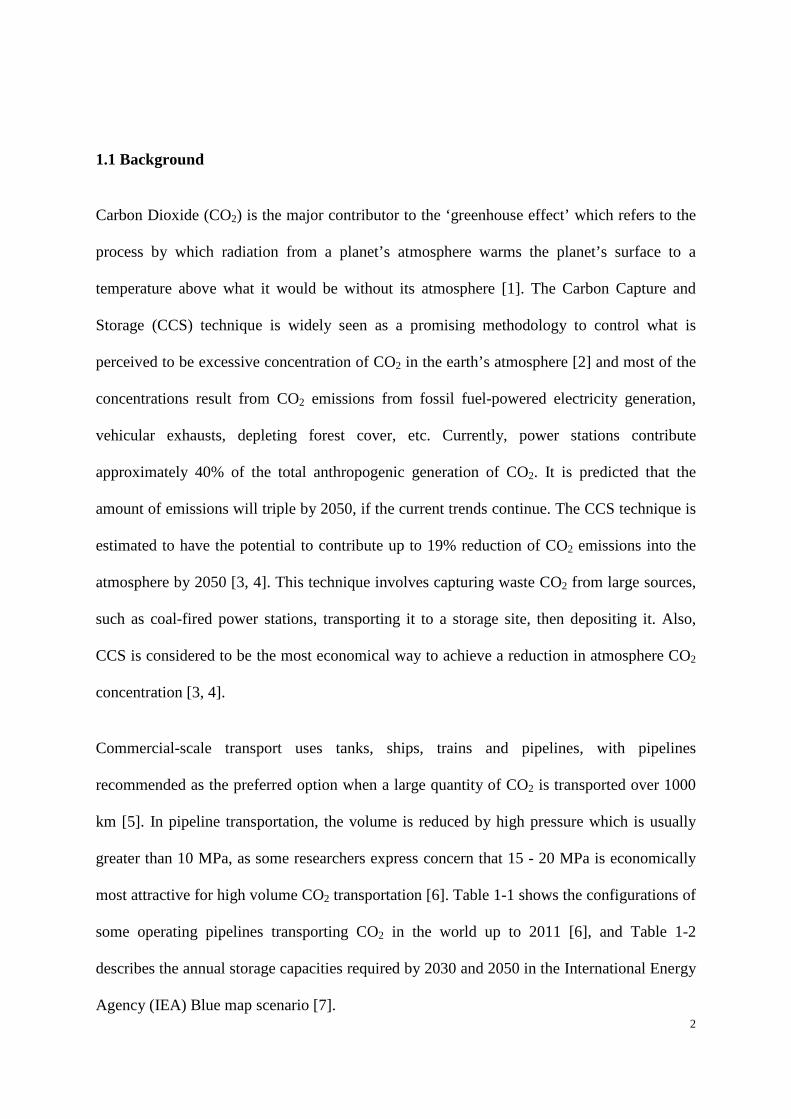
Carbon Dioxide (CO2) is the major contributor to the ‘greenhouse effect’ which refers to the

process by which radiation from a planet’s atmosphere warms the planet’s surface to a

temperature above what it would be without its atmosphere [1]. The Carbon Capture and

Storage (CCS) technique is widely seen as a promising methodology to control what is

perceived to be excessive concentration of CO2 in the earth’s atmosphere [2] and most of the

concentrations result from CO2 emissions from fossil fuel-powered electricity generation,

vehicular exhausts, depleting forest cover, etc. Currently, power stations contribute

approximately 40% of the total anthropogenic generation of CO2. It is predicted that the

amount of emissions will triple by 2050, if the current trends continue. The CCS technique is

estimated to have the potential to contribute up to 19% reduction of CO2 emissions into the

atmosphere by 2050 [3, 4]. This technique involves capturing waste CO2 from large sources,

such as coal-fired power stations, transporting it to a storage site, then depositing it. Also,

CCS is considered to be the most economical way to achieve a reduction in atmosphere CO2

concentration [3, 4].

Commercial-scale transport uses tanks, ships, trains and pipelines, with pipelines

recommended as the preferred option when a large quantity of CO2 is transported over 1000

km [5]. In pipeline transportation, the volume is reduced by high pressure which is usually

greater than 10 MPa, as some researchers express concern that 15 - 20 MPa is economically

most attractive for high volume CO2 transportation [6]. Table 1-1 shows the configurations of

some operating pipelines transporting CO2 in the world up to 2011 [6], and Table 1-2

describes the annual storage capacities required by 2030 and 2050 in the International Energy

Agency (IEA) Blue map scenario [7].

3

Table 1-1 Configurations of some operating CO2 pipelines [6]

Area Distance (km) Diameter of pipeline (m) Pressure (MPa)

USA and Canada >6000 0.3-0.7 10-20

Netherlands 85 0.65 1-2.2

Norway 245 0.32 20

Table 1-2 The annual storage capacities required by 2030 and 2050 [7]

Region 2030 2050

Africa 40 903

Australasia 129 353

Central + South America 52 476

Canada 148 574

China 307 2207

Eastern Europe 91 397

CIS 45 455

India 165 1153

Japan 42 129

Mexico 89 230

Middle East 60 505

Other Developing Asia 63 1093

South Korea 12 72

USA 495 1100

Western Europe 65.7 449.9

Total Mt/year 1802 10,097

4

Although in most cases, pipelines are very safe, if an accident occurs leading to release of

CO2 from a pipeline, the consequences may be catastrophic for human and animal

populations as well as the environment. This is because CO2 is colourless and odourless

under ambient conditions, and therefore escapes easy detection. But it is also an asphyxiant

gas that can lead to coma and even death at relatively high concentrations. Tolerable CO2

concentration without negative environmental impact is identified as 2,000 ppm [8]. For

humans, the Short Term Exposure Limit (STEL) of 15,000 ppm (1.5%) is used as a guide for

maximum exposure. This is the concentration below which no negative impact will be

observed on people after a 15-minute exposure [9]. Exposure levels above 10% will lead to

rapid loss of consciousness. Further exposure at higher concentrations leads to asphyxiation

[10]. Table 1-3 shows the health impact of CO2 at different concentration levels. As a result,

when using a pipeline to transport CO2, safety issues must be considered [11].

CO2 pipeline failures are usually caused by third party interference, corrosion, material

defects, operator errors and ground movement [12]. Overall, the failure rate of CO2 pipeline

ranges from 0.7 to 6.1 per 10,000 km per year [13]. The Australian pipeline design Standard

(AS 2885.1) has established parameters for ‘tolerable’ safety for pipelines transporting

hydrocarbon fluids, where the risk is related to the consequences of ignition of the released

fluid, and of the resultant fire. Methods for predicting the consequences of a fire are

reasonably well established, and human risk has been extensively studied. However, no

significant research has been undertaken to establish risk of fluid release from pipelines

transporting CO2. Therefore it is necessary to gain a better understanding of this process,

including depressurization in the pipe, atmospheric expansion and dispersion of CO2 released

from high-pressure pipelines in different scenarios. This will help develop controls that may

5

be needed to protect humans, animals and the environment from possible harmful effects of

pipeline failures.

Table 1-3 Health impact of CO2 [14]

Volume concentration Health effects

0.5% Long-term exposure limit in major jurisdictions

1% Slightly increased breathing rate

2% Doubled breathing rate, headache, tiredness

5% Very rapid breathing, confusion, vision impairment

8-10% Loss of consciousness after 5–10 minutes

>10% More rapid loss of consciousness, death if not promptly rescued

There are different measures to classify the patterns of failure. One of them is based on the

release direction. Because horizontal release is considered to be the worst case [13], most

research has focused on the study of horizontal release. Also, some studies show that the

vertical release pattern is quite different from the horizontal release pattern [15, 16]. Another

classification of the failure type of CO2 pipelines is based on the equivalent diameter of the

rupture, as shown in Table 1-4.

Table 1-4 Types of pipeline failure

Type Range of equivalent diameter (mm)

Full-bore pipe rupture > 150

Large leaks 50 to 150

Medium leaks 10 to 50

6

Small leaks 3 to 10

CO2 can present its state in four different phases – solid, gas, liquid and supercritical/dense

phase, and the phase diagram of CO2 is shown in Figure 1.1. Researchers [17-20], more often

than not, argued that two phases could co-exist on the boundaries between these phases and

three phases can co-exist at the triple point. Above the critical pressure (72.9 atm) and

temperature (31.1 ℃), CO2 presents in a supercritical state, in which it has both liquid density

and gas behaviours. In CCS projects, CO2 is most likely to be transported in a supercritical

state or liquid due to allowed smaller pipeline diameter and higher flow rates [21], thus phase

change process tends to be involved when CO2 discharges from a pipeline.

Figure 0.1 Phase diagram of CO2

Figure 1.2 shows the consequence of CO2 released from a high pressure pipeline. In terms of

a horizontal release, after the rupture of a high pressure pipeline filled with dense CO2, a

decompression wave is initiated inside the pipe and the velocity of this decompression wave

7

is nearly at the speed of sound. Meanwhile, in the vicinity of the exit, an under-expanded jet

flow exits from the orifice into the ambient with very high moment. This area which is

regarded as ‘the near-field’ expansion may be dominated by the initial momentum of the jet.

After travelling for a certain distance, the pressure will reach atmosphere pressure, and CO2

will disperse in to the atmosphere. In this region, the cloud will lose its initial momentum and

be effectively mixed with air, and disperse as a ‘Gaussian’ cloud. In this process, different

terrain types and meteorological conditions may significantly affect the dispersion profile of

CO2. Overall, the important factors that affect the dispersion of CO2 are the source ‘strength’

or mass flow rate (determined by the jet diameter, the direction and momentum of the release,

and the vapour mass fraction), terrain types and meteorological conditions. In order to obtain

a deeper understanding of the risk associated with the deployment of CO2 pipelines, a

dispersion model correctly reflecting the above aspects is essential.

Figure 0.2 Process of a CO2 release

1.2 Research objectives and activities

Generally speaking, no significant research has been undertaken to establish the risk

associated with CO2 release. The aim of this study is to establish a model and provide a basis

Inside the pipe Expansion Dispersion in atmosphere

8

for the development of rules involving with the whole process of the consequence associated

with CO2 pipeline release.

In order to achieve this aim, the whole process (as shown in Figure 1.2) will be divided into

three parts, namely Decompression, Expansion and Dispersion, as shown in Figure 1.3. The

three parts have their own characteristics and will be comprehensively studied in detail in this

study.

Figure 0.3 Schematic of problem partition

In the study of the depressurisation part, the main concern is fracture propagation, which is

one of the key issues for the design and operation of pipelines, as the need to arrest a running

fracture in a pipeline is paramount to the safety of a pipeline’s operation. Due to the tendency

of phase change and particular nature, such as usually including impurities, previous studies

showed that pipelines transporting CO2 would be more susceptible to running-ductile fracture

than one carrying natural gas [22]. One aspect of the design is to avoid running-ductile

fracture, which necessitates accurate models to predict the depressurisation behaviour when

the fracture occurs. Fracture propagation in fluid pipelines is commonly treated using the

semi-empirical Battelle Two-Curve Model (BTCM) [23, 24] where the aim is to estimate the

resistance of the material to rapid crack propagation. This method involves the superposition

of two independently determined curves: the fluid decompression wave speed and the

Pipeline Exit P0, T0 Pe, Te, ue, ρe Pa, Ta, ua

Expansion Depressurisation (inside the pipe) Dispersion (far-field)

Rupture plane

9

fracture propagation speed (the ‘J curve’), each expressed as a function of pressure. Figure

1.4 displays a schematic representation of the BTCM. The shape of the fluid decompression

wave speed curve depends on the phase of the fluid, as shown by the red and green curves in

Figure 1.4. Curves 1 and 2 represent the fracture speed curves for a given pipe diameter, wall

thickness, material, and two different toughness values. When the two curves intersect (i.e.

fracture curves 2 with the two-phase decompression characteristics), the fracture and fluid

decompression wave move at the same speed, but here the fluid pressure at the tip of the

fracture no longer decreases, which extends the fracture propagation distance. The boundary

between arrest and propagation of a running fracture is represented by tangency between the

decompression wave speed curve and the fracture speed curve. According to the BTCM, the

minimum toughness required to arrest the propagation of fracture is the value of toughness

corresponding to this condition [23, 24]. Clearly, as for two-phase decompression, the curve

of decompression wave speed vs pressure contains a plateau caused by phase change. The

existence of the plateau in the decompression curve will result in the curve (curve 1) left shift

markedly. Therefore higher toughness is required for the pipelines. In addition, the gas

captured from industrial emission sources is not 100 % pure CO2 but contains a range of

impurities as a result of the treatment process, which has a significant influence on the

decompression due to the change in the phase envelope. Therefore, the pipe flow associated

with CO2 release is greatly distinctive.

10

Figure 0.4 Schematic of the BTCM

The other concern in this part is to obtain the flow conditions at the Exit, such as Pe, Te, ρe, ue

and the discharge rate. Such data can also be treated as the inputs for predicting the

subsequent CO2 atmospheric expansion and dispersion. Therefore, an accurate pipe flow

model after rupture is crucial to the risk assessment of the CCS project.

The Expansion part determines the jet flow conditions at ambient pressure (Pa, Ta, ua) by

using the source strengthen at the Exit. The values of jet flow conditions are allowed to be

used as inlet boundary conditions for the Dispersion part.

The Dispersion part obtains the ‘radius’ of CO2, and in which the fluid can be treated as

incompressible. The influence of different conditions of operation and environment, such as

geography, weather conditions, and initial pipe pressure and so on, need to be focused on.

The major objectives of the work presented in this thesis are highlighted below:

Literature review: A comprehensive literature review focused on the models related to

prediction of the decompression behaviour of gas pipelines, expansion and heavy gas

dispersion is presented. Other aspects relating to this study are also included in the literature

Fracture or Decompression wave speed

11

review.

Development of a multi-phase decompression model: A multi-phase CO2 pipeline

decompression model available to both pure CO2 and CO2 mixture using CFD techniques is

presented in this research. The GERG EOS is employed to describe the properties of vapour

and liquid phases. A non-equilibrium phase change model using a mass transfer coefficient to

control the inter-phase mass transfer rate is implemented into the CFD code. By varying the

mass transfer coefficient, the effect of delayed nucleation on the decompression wave speed

can be investigated. Then optimum values of mass transfer for pure CO2 and CO2 mixture are

revealed. This model is also able to provide the discharge rate for the source strength study.

Development of models for source strength: Two methods are proposed to study the

necessary input (flow parameters at the inlet boundary) dispersion simulation. One is CFD,

which can provide more details. The other is an analytical model, which is applied to estimate

the atmospheric expansion. In this study, the discharge rate is predicted by the above models.

Development of heavy gas dispersion model: A deeper understanding of CO2 dispersion

resulting from accidental release is essential, and its dispersion patterns may vary according

to local and operational conditions. This part of the study focuses on CO2 dispersion under

different conditions.

CFD model validation: Several experiments carried out elsewhere are simulated to validate

the performance of the proposed modelling approaches.

In the following sections, a literature review is presented in Chapter 2. In chapters 3 and 4,

the multi-phase models regarding pure CO2 and CO2 mixture decompression are proposed,

respectively. In Chapter 5, Under-expanded CO2 jet is simulated. Results of simulation of

CO2 dispersion over a complex terrain are discussed in Chapter 6. The model for CO2 release

12

from high pressure pipeline is presented in Chapter 7. Finally, conclusions and

recommendations are presented in Chapter 8.

13

Chapter 2 Literature review

14

The published literatures relevant to the modelling of CO2 thermodynamic properties,

decompression, multi-phase model, source strength prediction and atmospheric dispersion are

reviewed in this section.

Nomenclature

A cross-sectional area f Darcy friction factor C mass transfer coefficient/concentration

c/w speed of shound Cdis discharge coefficient cp specific heat at constant pressure cv specific heat at constant volume

d/D diameter E energy fpc phase change energy ft ground heat flux

GCT critical flow rate per unit area H enthalpy/ buliding height h latent heat h0 stagnation enthalpy Hf volumetric heat transfer coefficient ID pipe internal diameter k kinetic energy M mass transfer rate P pressure Q mass flow rate q heat flux R universal gas constant r radius S entropy s0 stagnation specific entropy T temperature t time u velocity ur reference wind velocity V specific molar volume v velocity W decompression wave speed

15

x dynamic vapour quality X thermodynamic quality

xm The location of the Mach disc Subscripts

0 initial condition a atmosphere

amb ambient ave average b bubble line c critical e exit h hole l liquid

local local m mixture/mass-averaged n nozzle o observed p pipe/predicted p predicted

ref reference s/sat saturation

v vapour r reference

2.1 Equation of State

In physics and thermodynamics, an equation of state (EOS) is a constitutive equation which

provides a mathematical relationship between two or more state variables associated with the

matter, such as its temperature, pressure, volume, or internal energy.

Many different types of EOSs are used for the pipeline industry [25-27]. The use of a certain

EOS is dependent on the fluid region where calculation of the thermodynamic properties is

required. Modern work on the development of EOS to describe the pressure-volume-

temperature (PVT) behaviour of real gases can be traced to pre-industrialized Europe [27].

Robert Boyle and Edme Mariotte [27] measured the PVT behaviour of air at low pressures

16

and derived the inverse relationship between pressure and volume at constant temperature,

PV = kT, which is known as the Boyle-Mariotte Law. Later, Emile Clapeyron [27] combined

the equations of Boyle-Mariotte and Charles-Gay-Lussac to establish an EOS for a perfect

gas PV = R0T where R0 is a gas dependent constant.

In 1845, a substantial development was achieved when Victor Regnault developed an EOS

for ideal or ‘perfect’ gas [27, 28]. Victor Regnault applied Avogadro’s hypothesis on the

volume occupied by one mole of an ideal gas.

nRTPV = (2.1)

where n is the number of moles of gas and R is a constant called the universal gas constant

which is independent of gas type. This equation demonstrates the concept of a relationship

between pressure, temperature and density [28]. The ideal gas equation of state is roughly

accurate for gases at low pressures and high temperatures [28, 29]. However, at higher

pressures and lower temperatures such as the operation condition of natural gas pipelines,

ideal gas EOS becomes increasingly inaccurate, and fails to predict condensation from a

liquid to a gas under the depressurizing process [30]. Accordingly, work has concentrated on

ways to improve the ideal EOS.

For natural gas industry applications, many equations of state have been developed [27].

Most of them are an empirical or semi-empirical relationship, which is firstly based on the

ideal gas law and modified to conform to experimental data [29]. The use of a certain

equation depends on the fluid region where the calculation of the thermodynamic properties

is required [26]. These equations of state were initially limited to describe the pure substances

in either gas or liquid states [25]. Later, they were developed to describe the substance in both

the gas and liquid states, and consequently could be used to determine liquid-vapour

17

equilibrium such as the vapour fraction in the two-phase region, and the dew point and

bubble point curves [25, 31, 32]. Furthermore, the extension of equation of state from pure

substance to the correlation and prediction of the phase behaviour of a mixture is done using

mixing and combining rules [30]. The mixing rules are typically defined in terms of

combinations of binary mixtures. However, uncertainty inherent in experiments involving

mixtures is higher than that for pure substances [25]. Hence, an equation of state for mixtures

would be less accurate than one for pure substances [26].

2.1.1 RK EOS

Redlich and Kwong [33] proposed the RK EOS in 1949, which is an analytical cubic EOS.

Due to its relatively simple form, this EOS is still in use. The RK EOS is given as

( )bVVT

a

bVRTP r

+−

−=

5.0

(2.2)

C

r TTT = (2.3)

CPTRa

22

4274.0= (2.4)

C

C

PRTb 08664.0= (2.5)

where, Pc, Tc, P, R, V and T are the critical pressure, critical temperature, absolute pressure,

universal gas constant, specific molar volume and Kelvin temperature respectively.

Soave [31] proposed a three-parameter EOS, SRK EOS, which is modified from the RK EOS

18

and can predict the properties of CO2 in gas, liquid and supercritical state.

( )( )bVV

TabV

RTP r

+−

−= (2.6)

By letting:

22TRaPA = (2.7)

RTbPB = (2.8)

RTPVZ = (2.9)

the SRK EOS is written in cubic form as

( ) 0223 =−−+− BBAZZZ (2.10)

where Z is the compressible factor in this EOS and

2, )(4274.0

=

ci

ciri

TT

PP

TA ωα (2.11)

Ci

ci

TTPP

B 08664.0= (2.12)

The parameter αi(Tρ,ω) can be calculated by:

19

( ) ( )[ ]25.0, 11 riwr TmT −+=α (2.13)

2176.0574.148.0 iiim ϖϖ −+= (2.14)

2.1.2 Peng-Robinson EOS

Peng-Robinson EOS (PR EOS) is a cubic equation which is widely used in process

industries. The PR EOS is described by [34]:

22 2 bbVVa

bVRTP

−+−

−= (2.15)

with

222

)]/1(1[45724.0C

C

C TTP

TRa −+= κ (2.16)

C

C

PRTb 0778.0

= (2.17)

226992.054226.137464.0 ξξκ −+= (2.18)

where P is the pressure, T the absolute temperature, V the molar specific volume, R the

universal gas constant, ξ the ‘acentric factor’ of the gas (≈ 0.225 for pure CO2), and Tc and Pc

the temperature and pressure at the critical point respectively.

The PR EOS is widely used in the industry. The advantage of this equation is that it can be

accurately and easily represent the interrelationship between temperature, pressure, and phase

compositions in binary and multi-component systems. Implementation of the PR EOS only

requires the critical properties and acentric factor as inputs, and this EOS can only be used for

20

pure components. When calculating the properties of the mixtures, appropriate mixing rules

must be used. The Peng-Robins EOS is satisfactory for the gas phase, but not very accurate

for the liquid and gas pressure below the triple point.

2.1.3 Span & Wagner EOS

Span and Wagner [35] proposed a complex fundamental equation (approximately 50 terms),

which consists of a simultaneous nonlinear fit to all the available data of CO2. The

uncertainty of this equation ranges from ±0.03% to ±0.05% in density, ±0.03% to ±1% in the

speed of sound, and ±0.15% to ±1.5% in other parameters in the range from triple point to

523 K and 30 MPa for gas and liquid. But the Span & Wagner EOS is too complicated to be

used efficiently in CFD code. Furthermore, Span & Wagner EOS proved to be valid for both

the gas and liquid state above the triple point, but it does not take account experimental data

below the triple point, nor does it give the solid properties.

2.1.4 GERG EOSs

An EOS developed by the Groupe Européen de Recherches Gazières (GERG) in 2004 is

called the GERG-2004 EOS [26]. The GERG-2004 EOS is valid for wide ranges of

temperature, pressure, and composition and covers the gas phase, the liquid phase, the

supercritical region, and vapour-liquid equilibrium states for natural gases and other mixtures

consisting of up to 18 components: methane, nitrogen, carbon dioxide, ethane, propane, n-

butane, isobutane, n-pentane, isopentane, n-hexane, n-heptane, n-octane, hydrogen, oxygen,

carbon monoxide, water, helium, and argon.

The GERG-2008 EOS [36] [37] , the extended version of GERG-2004, considers three

additional components, n-nonane, n-decane, and hydrogen sulphide, resulting in a total of 21

components. The GERG-2008 EOS is able to represent the most accurate experimental

21

binary and multi-component data for the gas phase and gas-like supercritical densities, speeds

of sound, and enthalpy differences mostly to within their low experimental uncertainties.

• The normal range of validity of the GERG-2008 EOS covers temperatures of 90 K ≤

T ≤ 450 K and pressures of P ≤ 35 MPa. The uncertainty of GERG-2008 EOS in gas

phase density and speed of sound is less than 0.1% in the temperature range from 250

K~270 K to 450 K at pressures up to 35 MPa. This uncertainty is valid for various

types of natural gases as well as for many binary and other mixtures consisting of the

21 natural gas components covered by GERG-2008 EOS.

• In the liquid phase, the uncertainty of GERG-2008 EOS in density amounts to less

than 0.1%-0.5% for many binary and multi-component mixtures. The estimated

uncertainty in the liquid phase (isobaric) enthalpy differences are less than 0.5% to

1%.

• The Vapour-Liquid Equilibrium (VLE) is described with reasonable accuracy.

Accurate vapour pressure data for binary and ternary mixtures consisting of the

natural gas main components are reproduced by GERG-2008 EOS to within their

experimental uncertainty, which is approximately 1% to 3%.

Although GERG is considered as the standard EOS, the information from GERG may be

misleading in some cases for CO2 mixture. The speed of sound between the bounds of the

pressure (the dew line and the bubble line) is calculated by isentropic pressure variation with

the density. However, as for the mixture of vapour and liquid, speed of sound is probably

influenced by the interaction of the phase [38].

2.1.5 Composite EOS

22

Wareing et al. [39] proposed a composite EOS for CO2, where Peng-Robinson EOS is

applied to model the properties of gaseous CO2, and the properties of the liquid phase and

saturation pressure were calculated from tabulated data generated by the Span & Wagner

equation and DIPPR 801 database [40]. For the solid state, they used the relationship between

the property and temperature.

2.1.6 Comparison of EOSs

To date, the ability to accurately predict the VLE, the density and speed of sound is usually

considered the best way to gauge any weaknesses or strengths of an EOS [41]. Some

researchers compared different EOSs. Li and Yan [41] evaluated serval EOSs, including PR,

SKR and so on, for predicting the VLE of CO2 and CO2 binary mixtures, based on

comparisons with collected experimental data. Also, they compared different EOSs for

density [42]. The found that certain EOS tended to be superior in calculations on some

aspects. For example, PR EOS was recommended to calculate CO2/CH4 and CO2/H2S VLE.

Botros [43-47] predicted the speed of sound for different mixtures using different EOSs

based on the shock tube tests. It has been found that the GERG EOS outperformed the others.

Currently, the ideal gas EOS is built into most of the commercially available CFD codes, and

it can be used for the CO2 dispersion. But it is not appropriate to be used in the prediction of

CO2 decompression, as it may produce significant discrepancy at high pressure or low

temperature. The PR EOS can be used for the simulation of pure CO2 in the gaseous phase, as

it has a simple form and proven accuracy in the modelling of CO2 properties, but there are

some discrepancies when using this EOS to predict the properties of liquid phase CO2. Span

& Wagner EOS has high precision and it is suitable for predicting the properties of pure CO2

rather than that of a CO2 mixture. The GERG-2008 EOS can be applied for the modelling of

pure CO2 as well as mixtures. The components supported by GERG-2008 EOS cover the

23

components found in current CO2 mixtures. The GERG-2008 EOS will be used in the

simulation of the decompression process in the present study.

2.2 CO2 Pipeline decompression

One of the key requirements for CCS is fracture control. The determination of the required

toughness for the arrest of ductile fracture requires knowledge of the decompression

behaviour of the fluid. This requires accurate knowledge of its features, and according to

BTCM, one of the most important features is the decompression wave speed.

When a pipeline rupture occurs, a leading decompression wave propagates away from the

rupture plane into the undisturbed compressed fluid at the local speed of sound. The velocity

of decompression wave is a crucial parameter in pipeline fracture control philosophy [48].

The propagation of ductile fracture is closely linked to the decompression characteristics of

the pressurising medium [47, 49-53], and therefore, the driving force required to cause the

ductile fracture to propagate is derived from modelling the decompression wave velocity of

the escaping fluid [47, 50, 54]. The driving force for ductile fracture propagation in high

pressure pipelines is defined as the residual pressure of escaping fluid, which acts on the

inside wall of the pipe in the opening flap region [47, 52, 55].

2.2.1 Shock tube tests

In order to study decompression behaviours, a few full scale fracture propagation tests of

natural gases have been conducted by the European Pipeline Research Group (EPRG), British

Gas Corporation, Centro Sviluppo Materiali (CSM), and Battelle Institute, during the 1970s

[51, 56-59]. However, these kinds of full scale burst tests were enormously costly. Therefore,

in attempting to study the behaviour of pipe flow associated with high pressure pipe releases

economically, several shock tube tests of pure CO2 and CO2 mixture were carried out instead

24

of a full scale burst test.

The shock tube consists of spool pieces of steel pipe and a compression station [60]. The

experiment can ideally adjust the pressure and the temperature such that different

decompression paths can be observed. The sudden decompression is triggered by a rupture

disc calibrated to burst at a precise pressure [60]. This consumable disc is placed in a holder

at an extremity of the shock tube. Upon rupturing, the decompression wave propagates

towards the other end of the tube. The propagation is monitored through time by a series of

high frequency response pressure transducers placed along the tube at known intervals.

In shock tube tests, the decompression wave speed is usually determined from pressure-time

traces measured by transducers mounted at different locations along the pipe section [19, 20,

25, 43-46, 48, 49, 61, 62]. For any pressure level below the initial pressure, the time of arrival

of the decompression wave at each successive pressure transducer can be determined, and the

corresponding propagation wave speed W can be calculated using a linear fit of distance from

initiation against arrival time [48]. Such calculations are repeated for progressively lower

pressures, and the results presented in terms of a function of pressure p [48, 62]. The

decompression wave speed W is calculated by determining the times (t) at which a certain

pressure level is recorded at several pressure transducers at known locations (x) on the pipe

wall. By plotting these locations against time, the decompression wave speed could be

obtained by performing a linear regression of each isobar curve. The slope of each regression

represents the average decompression wave speed for each isobar. Therefore, the average

decompression wave speed (Wave) can be calculated by:

25

txWave d

d= (2.19)

Drescher et al. [63] conducted a shock tube test for depressurization of CO2-N2 mixtures. The

volume fractions of N2 were 10, 20 and 30 respectively. The experiment initial conditions

were approximately 12 MPa and 293.15 k for all cases. The tube used was about 140 m long

and the internal diameter was 10 mm.

Cosham et al. [64] have performed 14 shock-tube experiments for dense/liquid phase pure

CO2 and CO2 mixtures with impurities (H2, N2, O2, CH4). The length of the main section of

“pipeline” was 144 m and the internal diameter was 146.36 mm. The initial conditions ranged

from 3.89 MPa to 15.4 MPa and from 273.25 k to 308.75 k.

From 2001 – 2016, Botros et al. [48, 61, 65-71] performed a host of shock tube tests

including CO2 test and modelled the decompression behaviour of gas pipelines. In the most

recent tests, the main section of the shock tube was 42 m long and the internal diameter (ID)

was 38.1 mm. The tube was fitted with fluid and the rupture disc was at the front end of the

shock tube. At the time of cutting of the rupture disc, the pipe was opened to the atmosphere

and a decompression wave propagated up the tube. Tests were conducted with initial

pressures ranging from 10 to 30 MPa, and involving pure CO2 and CO2 with a range of

mixtures. The main section of the pipe had an extremely smooth surface, in order to minimize

frictional effects and to better simulate the behaviour of larger-diameter pipelines.

2.2.2 Decompression models

Behind the leading decompression wave, the local decompression wave velocity (Wlocal) is

the local speed of sound (c) minus the escaping out flow velocity (u) as described by [47, 59].

ucWlocal −= (2.20)

26

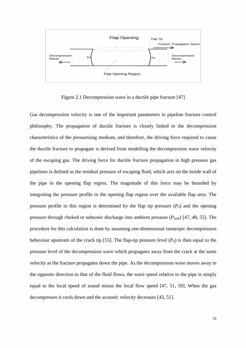
Figure 2.1 Decompression wave in a ductile pipe fracture [47]

Gas decompression velocity is one of the important parameters in pipeline fracture control

philosophy. The propagation of ductile fracture is closely linked to the decompression

characteristics of the pressurising medium, and therefore, the driving force required to cause

the ductile fracture to propagate is derived from modelling the decompression wave velocity

of the escaping gas. The driving force for ductile fracture propagation in high pressure gas

pipelines is defined as the residual pressure of escaping fluid, which acts on the inside wall of

the pipe in the opening flap region. The magnitude of this force may be bounded by

integrating the pressure profile in the opening flap region over the available flap area. The

pressure profile in this region is determined by the flap tip pressure (P0) and the opening

pressure through choked or subsonic discharge into ambient pressure (Pamb) [47, 48, 55]. The

procedure for this calculation is done by assuming one-dimensional isentropic decompression

behaviour upstream of the crack tip [55]. The flap-tip pressure level (P0) is then equal to the

pressure level of the decompression wave which propagates away from the crack at the same

velocity as the fracture propagates down the pipe. As the decompression wave moves away in

the opposite direction to that of the fluid flows, the wave speed relative to the pipe is simply

equal to the local speed of sound minus the local flow speed [47, 51, 59]. When the gas

decompresses it cools down and the acoustic velocity decreases [43, 51].

Flap Opening

Decompression Waves

DecompressionWaves

Flap Opening Region

Flap Tip

Fracture Propagation Speed

Po Po

27

For the calculation of the decompression wave speed, some models have been developed [19].

Most of these models are based on 1-D axial flow theory [72]. Groves et al. [51] developed a

computer program to calculate the gas decompression velocity using a similar approach of

shock tube theory at the University of Calgary, Alberta, Canada. This model adopted the

Soave-Redlich-Kwong EOS to determine the required thermodynamic properties. Groves et

al. validated their model against an expansion tube test results [44].

The most widely used model is GASDECOM [19, 47, 48], which wasoriginally developed

for calculating the decompression curve of hydrocarbons [49]. It has the capability of

modelling mixtures of hydrocarbons including nitrogen, carbon dioxide and methane through

to hexane. The model uses Benedict-Webb-Rubin-Starling (BWRS) EOS, with modified

constants known to give accurate estimates of isentropic decompression behaviour.

GASDECOM has been accepted to predict the decompression curve for natural gas as it is

validated against the measured results of full scale fracture propagation tests and shock tube

tests. In GASDECOM, the decompression wave speed (W) is calculated using Eq. (2.20).

Incremental pressure and densities are used to calculate the speed of sound c and the outflow

speed of the escaping gas u. The outflow speed u at any given pressure is the sum of

incremental Δu determined from:

( )s

uu ∑ ∆= 2

12

ρ

ρ (2.21)

Where

( ) ( )ρρ s

s cu ∆=∆ (2.22)

and ρ is the mass density, the subscript s indicates a value in the isentrope. The BWRS EOS

28

is used to calculate thermodynamic properties of the gas (speed of sound and density) in

GASDECOM. The speed of sound c is calculated by

Sddpc |ρ

= (2.23)

A number of assumptions are implicit within GASDECOM:

• One-dimensional frictionless isentropic flow is assumed and transient Navier-Stokes

mass, momentum, and energy balance equations expressed in terms of fluid velocity,

density, and pressure, in conjunction with a ‘real gas’ EOS to model pipe flow.

• If evaporation happens, the fluid is considered to remain at thermal and mechanical

equilibrium during depressurisation, with possible non-equilibrium phase transition

ignored.

• The rupture of the pipe is instantaneous, and the fluid is inviscid.

• Evaporation occurs instantly at the intersection of the pressure-temperature trajectory

with the two-phase envelope;

• The pipe is of sufficient diameter that no heat transfer or wall effects occur over the

timescale of interest in fracture propagation.

• No velocity slip occurs between vapour and liquid phases, mixture properties are

based on weighted average.

Several models have followed the approach of GASDECOM for fracture propagation studies

[19]. The difference between these models was the use of EOS [13].

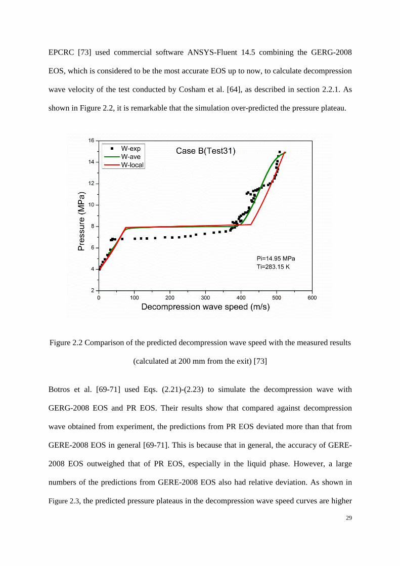
29

EPCRC [73] used commercial software ANSYS-Fluent 14.5 combining the GERG-2008

EOS, which is considered to be the most accurate EOS up to now, to calculate decompression

wave velocity of the test conducted by Cosham et al. [64], as described in section 2.2.1. As

shown in Figure 2.2, it is remarkable that the simulation over-predicted the pressure plateau.

Figure 2.2 Comparison of the predicted decompression wave speed with the measured results

(calculated at 200 mm from the exit) [73]

Botros et al. [69-71] used Eqs. (2.21)-(2.23) to simulate the decompression wave with

GERG-2008 EOS and PR EOS. Their results show that compared against decompression

wave obtained from experiment, the predictions from PR EOS deviated more than that from

GERE-2008 EOS in general [69-71]. This is because that in general, the accuracy of GERE-

2008 EOS outweighed that of PR EOS, especially in the liquid phase. However, a large

numbers of the predictions from GERE-2008 EOS also had relative deviation. As shown in

Figure 2.3, the predicted pressure plateaus in the decompression wave speed curves are higher

30

than those in the measured curves, which is similar to the EPCRC CFD prediction of shock

tube test with Cosham et al. [64].

0 100 200 300 400 500 6000

2

4

6

8

10

12

Experiment GERG-HEM

Pres

sure

(MPa

-a)

Decompression wave speed (ms-1)

Plateau

Trial 32A pure CO2

Figure 2.3 The comparison of decompression wave speed between measured and GERE-

HEM [69]

It was suspected that the discrepancies are introduced by the thermal equilibrium assumption

in this model, which is known as the Homogeneous Equilibrium Model (HEM) [74]. Hence a

flow model accounting for non-equilibrium phase transition is desirable. Some researchers

proposed to use a Homogenous Relaxation Model (HRM) [75, 76]. HRM comes from the fact

that an instantaneous thermodynamic equilibrium between two phases is not able to exist [77],

which is due to the finite rate of interphase mass transfer during phase change. A HRM

accounts for the delay in vaporisation during the decompression process using an empirical

relaxation equation. During the process of phase change, the pressure is not equal to the

saturation pressure and the local instantaneous quality fraction of each phase is usually

different from the value on the saturation line. This is the so-called delayed nucleation or

31

delayed bubble formation phenomenon during a high-pressure liquid state depressurisation

[78, 79]. To account for the non-equilibrium liquid/vapour transition, Brown et al. [80]

proposed a model by introducing a ‘relaxation time’, which was empirically determined by

Angielczyk et al. [81] based on tests involving the steady flow of CO2 through a nozzle. In

their study, Peng-Robinson (PR) EOS [82] was employed to model the fluid physical

properties. Prediction of a CO2 pipeline full-bore rupture test showed reasonably good

agreement with experimental data. However, it was found that the results were strongly

dependent on the relaxation time. Also, the improvement against HEM is limited and the

optimum relaxation time for CO2 depressurisation remains unrevealed.

2.3 Source strength prediction models

Apart from obtaining the decompression wave speed, as part of the safety assessment, the

hazards associated with accidental CO2 pipeline failure must be quantified and appropriate

mitigating steps must be taken to bring their consequences to acceptable levels [79].

Accordingly, obtaining the parameters at the pipeline outlet, including the outflow rate,

pressure, temperature and fractions of each fluid phase plays an essential role. Such data can

also be treated as the inputs for predicting the subsequent CO2 atmospheric expansion and

dispersion. Therefore, an accurate prediction of time-varying discharge rate (source strength)

is crucial to risk assessment of the CCS project.

Before releasing (assumed full-bore), the stagnation pressure in a CO2 pipeline is usually at

higher saturation pressure. At the moment of rupture, the pressure at the outlet drops firstly to

the choke pressure, and the rest of the pipe also starts to depressurise. To precisely predict the

time-varying discharge rate, an understanding of the details of the depressurisation process

inside the pipeline is required.

32

2.3.1 Equation for the choked exit condition

A computer model for predicting leak rates of chemicals from damaged storage and

transportation tank leakage was proposed by Belore and Buist [83]. It can be used to calculate

the process of gas released from a hole in a tank. This model could also be used to estimate

source terms of high pressure gas pipeline leakage. It was suggested that the flow could be

either subsonic or supersonic depending on three ratios. The first important parameter was the

ratio of atmospheric pressure (Pa) to tank pressure (P0),

0/ PPR aP = (2.24)

The second important parameter was the hole-to-tank length scale ratio given by

thc LL /=β (2.25)

In terms of a pipeline with a circular hole, Lh=2rh, Lt=2rt, where rh is the radius of the hole, rt

the radius of the pipeline.

The third important variable was a ‘critical’ pressure ratio, Rc, whose value depends on βc:

≤+

=−

+

>

+

=

−

−

)holesmall(2.02

12

1

)holebig(2.01

2

24

1

1

cccc

cc

RR

R

βgβg

βg

ggg

gg

(2.26)

where g =cp/cv is the ratio of specific heats for the fluid.

If Rp≤Rc, the flow at the exit plane is usually chocked, indicating that further reduction of

downstream pressure does not change the flow rate appreciably. The mass flow rate is given

by

33

11

0dis 12)()()(

−+

+

=gg

ggρ tPtACtQ e (2.27)

where Cdis is discharge coefficient; Ae the discharge rupture opening cross-sectional area.

The applicability of Eq. 2.28 relies on an estimation of the time-varying fluid density,

pressure and ratio of specific heats, which are related to the EOS and the decompression

process. This equation has been usually used to predict a very conservative initial release rate,

applying stagnation values for variables on the right side of the equation.

2.3.2 Wilson’s method [84]

Wilson [84] assumed that the gas released from pipeline rupture was almost entirely

isothermal. Measurements showed that heat transfer to the moving gas through the pipe walls

maintained an almost isothermal condition throughout the length of the pipe except for

approximately the last 200 diameters of the hole. Over the latter distance, the flow was

assumed to be adiabatic because of the large acceleration near the end of the pipe.

Wilson showed that the release rate for an isothermal, quasi-steady state pipe flow could be

adequately described by:

( )ββα αα

//0 2

)1()( tt eeQtQ −− +

+= (2.28)

where Q(t) is the mass flow rate as a function of time, Q0 is the initial mass flow rate at the

time of the rupture, α is a non-dimensional mass conservation factor and β is the release rate

time constant. As the initial pressure in pipeline is usually much greater than the ambient

pressure, Q is calculated using Eq. 2.27, assuming a choked flow condition, Cdis=1, initial

temperature and pressure, and gas constants at the time of rupture.

34

This model can predict time-varying release rate, but it uses the equation for choke condition

to obtain the initial release, thus its validity is limited. Also, the value of mass conservation

factor and release rate time constant may significantly affect the prediction of time-varying

release rate.

2.3.3 Morrow model [85]

Morrow proposed a pipeline break flow model for estimation of the time-dependent flow rate

of Liquefied Petroleum Gas (LPG) from a pipeline rupture [85]. The correlation of pressure

just inside the pipe exit and flow rate during choked flow is defined as follows:

[ ]

+−−

++−+−−=

22

dd

22422dd1

Xvv

Xvv

XPv

XvXvvvXvvvPX

G

g

f

g

fg

gfgfgffCT

(2.29)

where GCT is the critical flow rate per unit area, P the pressure, X the thermodynamic quality,

vf the specific volume of saturated liquid, vg the specific volume of saturated vapour.

The rate of change of thermodynamic quality with respect to pressure is given by

++−=

PvU

vX

Ph

XPh

hPX gf

f

fgf

fg dd

2dd

dd1

dd 2

(2.30)

where hfg is the latent of vaporisation, hf the specific enthalpy of saturated liquid and Uf the

velocity of liquid phase.

In principle the Morrow model was developed for LPG outflow from a pipeline, however,

with use of the proper physical properties it can be applied to other substances also. In

addition, its performance also relies on the prediction of thermodynamic properties of the

35

fluid.

2.3.4 Phast modules

DNV Phast is a comprehensive hazard analysis software tool, which can examine the

consequences of a potential incident from the initial release to far-field dispersion, and is

commonly used in the process industry [86]. Phast provides the DISCharge module DISC

(steady-state calculations based on initial mass flow rate) and Time-Varying discharge

module TVDI.

DISC [87] can simulate the release from a small rupture opening in a vessel. It is an initial-

rate discharge model, which predicts the worst-case initial discharge rate and the duration

associated with this discharge rate. The fluid stored in the vessel may be vapour, liquid or

two-phase.

Assuming that the fluid in the vessel is initially stagnant:

2

2

0e

euhh += (2.31)

where h0 is the stagnation enthalpy and he the enthalpy at the exit respectively, and ue is the

fluid velocity at exit.

Assuming an isentropic flow:

ess =0 (2.32)

where s0 is the stagnation specific entropy and se the specific entropy at the exit. The rupture

opening pressure Pe equals the ambient pressure in case of an unchoked flow, and is

determined from the choke pressure in case of choked flow.

36

],max[ chokee PPP ∞= (2.33)

Here Pchoke is the choke pressure at the rupture opening and is defined as the pressure

corresponding to the maximum mass flux (mass flow rate per unit area) Ge, through the

rupture opening:

e

ee v

uG = (2.34)

where ve is the specific volume, defined as

Ve

Ve

Le

Leev

ρη

ρη

+= (2.35)

where ηLe and ηVe are the liquid and vapour mass fraction respectively, ρLe and ρVe the liquid

and vapour density respectively.

Considering the rupture opening cross-sectional area Ae, the mass release rate Q is then:

ee AGQ = (2.36)

The equation represents an idealised (maximum) flow rate, but the frictional effect of

convergent flow at the rupture opening effectively reduces this. The convention is to estimate

this by assuming an effective (reduced) rupture opening cross-sectional area, using a

discharge coefficient, Cdis.

ee AGCQ dis= (2.37)

TVDI [88] estimates the release rate and containment conditions as functions of time

following a loss of containment event. The vessel may contain single or multi-phase fluids.

37

For multi-phase containment, the release could either occur from the vapour or liquid space

and may involve single or two-phase flow. TVDI is composed of two sub-models: the gas

(TVRGAS) and the multi-phase (TVEXEC /TVLEAK) vessel depressurisation models. Each

model accounts for the effects of isolation, inflow and outflow (including blowdown) on the

transient mass and heat transfer processes occurring within the boundaries of the “main”

vessel.

TVDI employs the DISC model to predict the discharge rate by assuming time-dependent

stagnation pressure and temperature. For multi-phase discharge modelling, TVDI considers

the internal mass transfer (evaporation from liquid to vapour phase) as well as external mass

transfer (mass lost due to discharge through the rupture opening leak/ pipe rupture). The mass

conservation for the entire system is defined as:

)](),([d

d00DISC tTtPm

tM

−= (2.38)

where ṁDISC is the flow rate calculated using the DISC model at the time-dependent

stagnation pressure P0(t) and T0(t).

Mass conservation is also applied to each phase that is potentially present in the vessel:

)](),([)(d

dd

d00DISC

, tTtPmtxt

Mt

ML

LevapL −−= (2.39)

)](),([)(d

dd

d00DISC

, tTtPmtxt

Mt

MV

LevapV −= (2.40)

where x is the mass fraction at the rupture opening of a particular phase. Subscripts L and V

indicate the liquid and vapour phase respectively.

38

The energy balance for the system is then given by

( )

)()(d

)()(dtEtE

ttTtH

outincap −= (2.41)

where Hcap is the ‘heat capacity’ of the system, T is the system temperature (thermal

equilibrium assumed throughout the vessel), while Ėin and Ėout are the rates of energy going

in and out of the system respectively.

The mass and energy balances are coupled with Raoult’s and Dalton’s laws. First, Raoult’s

law for an ideal solution gives the partial vapour pressure of component i, Pi(t):

)()()( ,, tytPtP iLsat

iVi = (2.42)

where PVsat is the saturated vapour pressure of component i at temperature T(t) and yL,i is the

mole fraction of component i in the liquid phase. Then Dalton’s law of partial pressures can

be used to obtain the total pressure P(t):

∑∑−≠−≠

=compcomp N

econdensablnonkiV

N

econdensablnonki tytPtP )()()( , (2.43)

where yV,i is the mole fraction of component i in the vapour phase and Ncomp is the total

number of components (condensable and non-condensable) in the vapour phase.

Models used by Phast are comprehensive and are widely used in industry. Currently Phast

supports three EOS: PR, SRK and Phast Multi-Component. It does not support GERG, which

is widely considered to be the best EOS for CO2.

2.3.5 EPCRC model

39

This model [89] is a decompression wave speed model developed by the Energy Pipelines

Cooperative Research Centre (EPCRC). EPCRC model solves the following one-dimensional

dynamic differential equations using the finite difference method. Eq. 2.45 is derived

assuming that the ‘outflow’ speed and pressure are constant along the pipe radial direction.

The decompression process is supposed to be isentropic, while the frictional effects are

accounted for using a friction factor:

02

)( 2 =−∂∂

−+∂∂ u

Dwf

xPuw

tP ρ (2.44)

where w is the speed of sound, u the ‘outflow’ speed, t the time, x the distance from the

rupture, f the Darcy friction factor and D the pipe diameter.

In addition, the speed of sound w, the density ρ and the temperature T are obtained from the

GERG-2008 EOS. The thermodynamic quantities are expressed as functions of the pressure

P and the specific entropy s.

ρρ∂

=∂ wu (2.45)

s

Pwρ∂

∂= (2.46)

),( sPρρ = (2.47)

),( sPTT = (2.48)

Based on the fluid state (P, T, ρ, w, u) at (t, x), a finite difference scheme of Eq. 2.45 is used

to evaluate the pressure field as a function of time. Following a flash point calculation of the

density for the updated pressures, the velocity of the flow is achieved using Eq. 2.46. As The

EPCRC model employs the GERG-2008 EOS, the thermodynamic properties of the mixture

40

can be precisely represented, leading to good prediction of decompression wave speed [42].

Also, the choke conditions at the rupture opening can be precisely predicted. Although the

EPCRC model was not originally designed for the estimation of release rate, the predicted

choke condition can be used to calculate the release rate. The EPCRC model directly solves

the dynamic differential equation and uses GERG-2008 EOS to predict the thermodynamic

properties. However, the influences of ‘delayed nucleation’ have not been considered in this

model.

2.4 Expansion to atmospheric pressure

Fluid released from a high-pressure pipeline will be immediately followed by an under-

expanded jet flow exiting from the rupture opening into the ambient with very high

momentum. Usually the flow structure features a Mach disc, corresponding to a normal shock.

Upstream of the Mach disc the flow is supersonic, while downstream of the Mach disc the

flow is subsonic. The location of the Mach disc can be empirically determined by [43]:

∞

=PPdx em

06455.0 (2.49)

where de is the diameter of the rupture opening.

The region between the rupture and the Mach disc is the expansion zone shown in Figure 1.3.

Downstream of the Mach disc, the jet pressure will reach the ambient pressure. Having

obtained the source strength at the rupture opening, the jet conditions at ambient pressure can

be used as inlet variables for the subsequent dispersion modelling. The fluid in the dispersion

model can be treated as incompressible and the supersonic region can be removed.

Birch et al. [90] assumed firstly that viscous forces are negligible over the expansion surface,

41

and secondly that there is negligible entrainment of ambient air. With these assumptions, the

equations for conservation of mass and momentum can be written as

disCuAuA eeeaaa ρρ = (2.50)

and

)(2dis

22aeeeeeaaa PPACuAuA −+= ρρ (2.51)

where subscripts e and a denote variables at the exit plane and atmospheric plane respectively.

Solving these equations for ua and Ae, one can obtain:

disdis )( CuPPCuu eeaeea ρ−+= (2.52)

and

)( 2dis

22dis

22 CuPPCAuA eeaeaeeea ρρρ +−= (2.53)

Birch et al. also assumed the fluid will rapidly regain its original stagnation temperature, so

that Ta≈T0. Thus the density of the fluid at the atmospheric plane can be obtained using an

appropriate EOS.

Sand et al. [91] assumed negligible body forces, air entrainment and viscous forces in the

expansion zone. From the ideal gas EOS and the conservation equations for mass, momentum

and specific enthalpy they get:

42

)()( eeaeea uPPuu ρ−+= (2.54)

( )22

21

aeea uuhh −+= (2.55)

( ) paeea cuuTT 22

21

−+= (2.56)

( )aaa RTP=ρ (2.57)

( )aaeeea uuAA ρρ= (2.58)

where R is the universal gas constant.

Phast provides an ATmospheric EXpansion module ATEX [87, 88, 92] to deal with the

expansion of a continuous release from the conditions in the leak rupture opening down to

atmospheric pressure. Along the expansion zone one-dimensional homogeneous flow is

assumed in thermal equilibrium and with zero air entrainment.

In the ‘conservation of momentum’ model, the unknown post-expansion data are set from the

pre-expansion data by imposing three conservation equations (conservation of mass,

momentum, and energy) and two equations of properties (equations for density and enthalpy):

eeeaaa uAuA ρρ = (2.59)

eaeeeeaaa APPuAuA )(22 −+= ρρ (2.60)

+=

+ 22

21);,(

21

eLeeeeeeeaaaaa ufTPhuAuhuA ρρ (2.61)

43

( )Laaaa fTP ;,ρρ = (2.62)

( ) ),()1(),(;, aaVLfaaLLaLaaaa TPhfTPhffTPhh −+== (2.63)

The isentropic model applies the same equations as the above model. However, instead of the

assumption of conservation of momentum, the isentropic model assumes that entropy is

conserved between the initial and final states, i.e. that the entropy at the end of expansion to

atmospheric pressure is the same as the entropy in the leak rupture opening.

( )Laaaee fTPsTPs ;,),( = (2.64)

Clearly, ATEX model is more comprehensive and it has the advantage of calculating phase

fractions. If the pressure and temperature at the rupture opening can be predicted, applying

the homogeneous equilibrium assumption, phase fractions at the rupture opening and the

ambient pressure plane can all be estimated.

2.5 Phase change models

2.5.1 The process of phase change during the release and dispersion

Because CO2 will be transported in dense phase, the phase change from liquid to vapour is

most likely to take place inside the pipe when pipelines rupture, with the decrease of pressure.

Accurate modelling of the multi-phase flow requires the reasonable phase change model

which can reflect the real inter-phase transfer process. One of the biggest challenges

associated with high pressure CO2 pipeline release is the correct modelling of this transition

from one phase to two-phase. Figure 2.4 illustrates pressure-enthalpy paths in different leak

cases [93] and it can be seen that different initial conditions will lead to various phase change

processes. The phase transition is an important character in the CO2 pipeline release. When

44

CO2 releases from the dense state (supercritical fluid) or liquid state, the expansion will

involve a phase change to vapour phase (‘flashing’). At the exit plane (the hole) or the

rupture opening, there will exist two phases - liquid and vapour (leaks 1, 2, 3, 4). Leaks 1 and

2 start with dense phase, and go through the processes pass liquid, liquid-vapour, and solid-

vapour regions but leaks 3 and 4 don’t go through a pure liquid region. In these conditions,

the expansion to equilibrium will generally take the jet conditions to the sublimation point at

1 bar, -78.5 ℃, with some mixture of vapour and solid. For leak 5, while the initial condition

is far above the critical temperature, occurring possibly during a compression process, the

CO2 changes its state from dense phase to gaseous phase directly. For CO2 release initiated

from the vapour state, and it may go through the liquid-vapour, solid-vapour regions (leak 6).

In addition, the solid CO2 can sublimate to the gaseous state.

Figure 2.4 Sketch of pressure – enthalpy paths in different leak cases

Overall, modelling the phase change of CO2 released from a pipeline plays an important role

in this study. However, up to now, there is not a pro-existing reasonable phase change model

Pres

sure

Solid-

Dense Phase

Solid-Vapour

Vapour

Enthalpy

Liquid Liquid-vapour

Leak 1

Leak 3

Leak 2 Leak 4 Leak 5

Leak 6

45

for CO2 in CFD codes. As mentioned above, the ignorance of the non-equilibrium

phenomenon probably causes discrepancy in terms of high pressure CO2 release. Therefore,

this study focuses on the HRM, which considering the relaxation during phase change.

Studies should be directed to this end and phase change models of other material may be

referred.

2.5.2 Phase change models based on temperature relaxation

Kumar et al. [94] studied a model for the surface evaporation using CFD package Fluent.

Liquid hydrogen (LH) was considered to be kept in insulated 2-D axial symmetrical

cylindrical tanks at a temperature of 20 K and atmospheric pressure, which absorbed the heat

through cylindrical walls. Mass and energy source terms were added to deal with the

interfacial mass and heat transfer. The computation results showed the thermal stratification

in tanks under different conditions. The model was deemed acceptable by comparing the

predictions with the experimental measurements.

Wei et al. [95] suggested a Volume of Fluid (VOF) method to model the bubble behaviours

in sub-cooled flow of boiling water using the CFD package Fluent. The effect of additional

inertial forces on energy and mass transfer during phase change was considered. The sub-

cooled water flowed in a 3-D rectangle domain with one heated wall. It appears that the water

might evaporate near the heated wall and the vapour might condense within some area where

the temperature was not high enough. To simulate the process of phase change in the

interface of liquid and vapour, they added a mass source term in the continuity equations and

a heat source term in the energy equation. If T ≥Tsat, the evaporation occurred, the mass was

transferred from the liquid phase to the vapour phase,

46

sat

satlll

TTTCM )( −−

=αρ (2.65)

If T< Tsat, the condensation occurred, the mass was transferred from the vapour phase to the

liquid phase

sat

satvvv

TTTCM )( −−

=αρ (2.66)

The time relaxation factors cl and cv were specified at 100 s−1 in order to numerically

maintain the interface temperature within Tsat ±1 K. They successfully obtained the vapour

area which was defined as the area where the volume fraction of vapour was greater than

50%, and the bubble’s behaviour was investigated as well. Compared with some bubble

behaviours obtained by experiment, the authors thought the model was successful.

Henczka et al. [96] proposed a model for spray-freezing of compressed CO2 using CFD

software, within which a solidification model of droplets was presented. Figure 2.5 shows the

definition of the physical domain for the drop freezing problem. They considered that the

process was featured by the existence of a moving interface between the solid phase and

liquid phase at which the thermal energy in the form of latent heat was liberated. They used

the method proposed by Wu et al. [97] and the model described by the one-dimensional

unsteady heat conduction equation for the solid shell R≤ r ≤RS

∂∂

+∂∂

=∂∂

2

22rT

rT

rtT

Sα (2.67)

with boundary conditions:

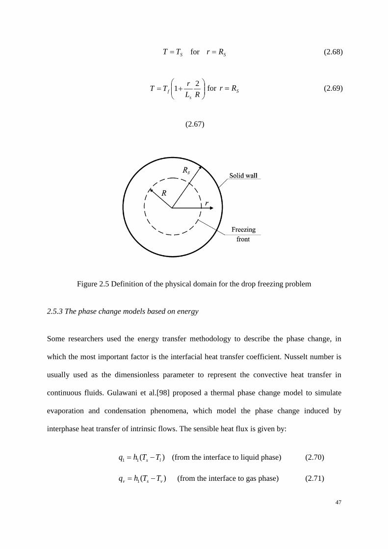
47

STT = for SRr = (2.68)

+=

RLrTT

sf

21 for SRr = (2.69)

(2.67)

Figure 2.5 Definition of the physical domain for the drop freezing problem

2.5.3 The phase change models based on energy

Some researchers used the energy transfer methodology to describe the phase change, in

which the most important factor is the interfacial heat transfer coefficient. Nusselt number is

usually used as the dimensionless parameter to represent the convective heat transfer in

continuous fluids. Gulawani et al.[98] proposed a thermal phase change model to simulate

evaporation and condensation phenomena, which model the phase change induced by

interphase heat transfer of intrinsic flows. The sensible heat flux is given by:

)(11 ls TThq −= (from the interface to liquid phase) (2.70)

)(1 vsv TThq −= (from the interface to gas phase) (2.71)

48

where hl and hg are the heat transfer coefficients for liquid and gas phase, respectively, which

is modelled by Ranz-Marshall Model

Nu = 2 + 0.6 Re0.6Pr0.9 (2.72)

So the total heat flux balance was given by

lsmHqQ += 11 (from the interface to liquid phase) (2.73)

vsvv mHqQ += (from the interface to vapour phase) (2.74)

The Hls and Hvs are the value of enthalpy carried into or out of the phases due to the phase

change. Because Ql + Qv = 0, the interphase mass flux is determined from the total balance as

follows:

lvs

vl

HHqqm

−+

= (2.75)

Ajmal et al. [99] divided the process of heat transfer between two phases into two steps -

from interface to liquid and from vapour to interface. The liquid phase Nusselt number is

calculated as [100]:

Nu = 2 + 0.6 Re0.5Pr0.33 (0≤Re<776.06, 0≤Pr<250) (2.76)

Nu = 2 + 0.6 Re0.062Pr0.33 (Re≥776.06, 0≤Pr<250) (2.77)

where Re = ρl|Ug-Uf| and Pr=cpul/kl

The volumetric heat transfer coefficient for the liquid phase is

49

Hf = hfAfg (2.78)

To avoid code failure caused by high condensation rates, the authors used the Mavko [101]

restriction as:

×−×−

×−= −

−

10

10

100.11.0100.1

,1min(,0max)]1(4.724472.4max[17539,min gggff HH

ααα (2.79)

2.5.4 Phase change models based on pressure relaxation involving with CO2

In the processes of decompression and expansion of CO2, some researchers thought the

vapour would only exist in an equilibrium state if the liquid droplets and solid particles were

sufficiently small, but some researchers indicated that this was not true. In terms of expansion,

Woolley et al. [102, 103] ignored the temperature relaxation and simply assumed the

condensed mass fraction as:

( ) vt Suut

=∇∇−∇+∂

∂ )( αραρα (2.80)

( )sat

satvv p

ppSt

β −= (2.81)

Where, ρ, ut, pv and psat are mixture phase density, turbulent diffusion coefficient, vapour

pressure and the saturation pressure, respectively. They firstly set the relaxation time t as 10-

3 s [102] and used the correlation as follows [103]

b

c

aSG

pppp

vvx

−−

=

0

00tt (2.82)

CO2 tends to change its state from gas to solid when releasing from high pressure pipelines.

50

Experiments showed that the process of de-sublimation was similar to the process of

condensing [104]. Cui et al. [105] proposed a CFD model to predict the vapour in the air frost

to ice on a fin-and-tube heat exchanger. A transient multi-phase multi-component flow model

with phase change was employed to describe the forced convection heat transfer. In this

model, the continuous moist air was set to the primary phase and the discrete ice droplet was

set to the secondary phase. The inter-phase mass transfer process between the water vapour

and ice was accomplished by adding a source term to the component transportation equation

for the primary phase. The latent heat due to phase change was considered by adding the

energy source term. The authors used this model to simulate several cases and obtained the

effects of temperature, flow rate and relative humidity on frost, and the transient local frost

formation. The average frost thickness, heat exchanger coefficient and pressure drop on air

side has been analysed as well.

Witlox et al. [106] discussed the modelling of the discharge and subsequent atmospheric

dispersion of CO2 releases using the consequence modelling package, Phast. Their work

involved extending the capability of the original Phast model to include liquid-to-solid

transition or vapour-to-solid transition. Phast examined the progress of a potential incident

from the initial release to the far-field dispersion including the modelling of rainout and

subsequent vaporization. The original Phast discharge and dispersion models allowed the

released chemical to occur only in the vapour and liquid phases. This applied both for the

post-expansion stage of the discharge model, as well as for the thermodynamic calculations

by the dispersion model. Solid property calculations were added where necessary. The above

extensions were generally valid for fluid releases including CO2. Using the extended

dispersion formulation, a sensitivity study has been carried out for mixing solid CO2 with air,

and it is demonstrated that solid effects may significantly affect the concentrations.

51

In terms of CO2 pipe flow, Brown et al. [80] proposed a model by introducing a ‘relaxation

time’, which was empirically determined by Angielczyk et al. [81] based on tests involving

the steady flow of CO2 through a nozzle, shown as Eq. 2.84.

t

xxzxu

tx eq −

=∂∂

+∂∂

(2.83)

where, x and xeq are the dynamic vapour quality and equilibrium vapour quality, t is a

relaxation time accounting for the delay in the phase change transition.

2.6 Dispersion models

In recent years, a number of models have been proposed to estimate the atmospheric

dispersion of gases resulting from accidental or planned release. These can be classified into

three categories: (a) “Gaussian-based” models, (b) “Similarity-profile” models, and (c)

Computational fluid dynamics (CFD) models [107].

2.6.1 “Gassian-based” models

An atmospheric dispersion model is typically used to estimate dispersion from a continuation

point source on the assumption that the plume is dispersed by homogeneous turbulence. The

model should contain the effects of advection (transport), and dispersion (including dilution

by the wind and dispersal due to turbulence) and possibly considerations of plume rise, wind

shear, and physical and chemical transformations. Turner [35] reviewed the historical

development of the atmospheric dispersion model. The advent of the first six ‘off-the-shelf’

computer models in 1973 in the USA was described. The first model was based on Gaussian

assumptions, and only applicable for primary pollutants. Salient points of current models

were examined. Possible sources or errors were pointed out, and the importance of validation

52

against experimental data was emphasised. The standard Gaussian formula is of the following

form when variables and parameters represent averages over about a one-hour time period.

+−+

−−

−=

222

21exp

21exp

21exp

2),,(

z

s

z

s

yzy

hzhzyu

QzyxCssssps

(2.84)

where sy and sz, called the ‘dispersion parameters’, are the standard deviations of C in the

cross-wind and vertical directions respectively. These dispersion parameters are functions

only of the downstream distance x. There are also some operational models, which are based

on the Gaussian dispersion model [108]. ERBRINK [109] proposed a practical model to

estimate the coefficients of σy and σz through fitting the experiment data. It seems that the

Guassian model was not very accurate. Hanna et al. [110] calculated the dispersion in Salt

Lake City and Los Angeles of SF6 and the results showed 70% - 300% errors compared to

the experimental data. Furthermore, Gaussian model fails to describe gas flow over complex

topography and to predict the dispersion of high speed releases. In addition, Guassian model

was established for lighter-than-air gas, but CO2 is a heavier-than-air gas. The behaviour of a

heavier-than-air gas cloud makes it dangerous for human safety, as it tends to fall to the

ground due to its negative buoyancy and to remain there at usually high levels of

concentration for comparatively long periods as opposed to neutral or positively buoyant

clouds. Overall, Gaussian model and the models based on the Gaussian model are 1-

dimensional time-independent equations and are not suitable to depict the dispersion over

complex terrains, or the terrain associated with high temperature, velocity or pressure

gradients.

2.6.2 “Similarity-profile” models

(1) SLAB

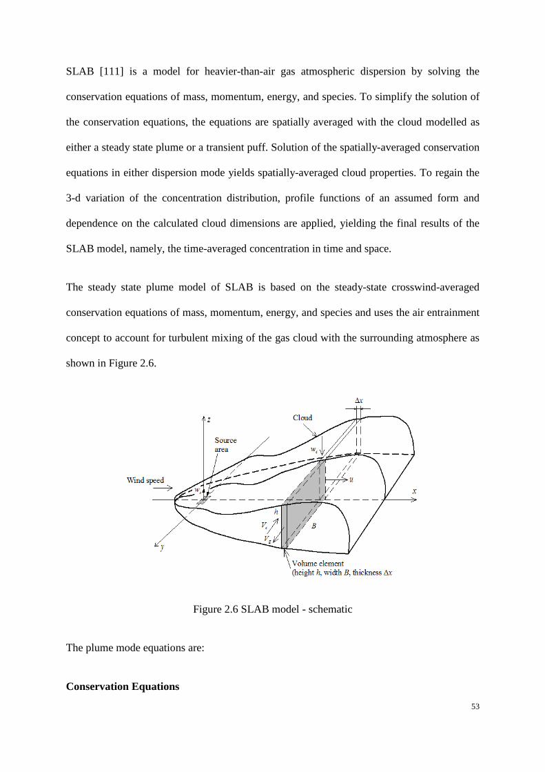
53

SLAB [111] is a model for heavier-than-air gas atmospheric dispersion by solving the

conservation equations of mass, momentum, energy, and species. To simplify the solution of

the conservation equations, the equations are spatially averaged with the cloud modelled as

either a steady state plume or a transient puff. Solution of the spatially-averaged conservation

equations in either dispersion mode yields spatially-averaged cloud properties. To regain the

3-d variation of the concentration distribution, profile functions of an assumed form and

dependence on the calculated cloud dimensions are applied, yielding the final results of the

SLAB model, namely, the time-averaged concentration in time and space.

The steady state plume model of SLAB is based on the steady-state crosswind-averaged

conservation equations of mass, momentum, energy, and species and uses the air entrainment

concept to account for turbulent mixing of the gas cloud with the surrounding atmosphere as

shown in Figure 2.6.

Figure 2.6 SLAB model - schematic

The plume mode equations are:

Conservation Equations

54

Species

xBwuBhm sss d/)(d)'(where,)'( == ρρ (2.85)

Mass

ssseea BwBwhVuBh ρρρ ++= )()'( (2.86)

Energy

tpcspssssapaeeap ffTcBwTcBwhVTuBhc ++++= ρρρ )()'( (2.87)

X-Momentum

uaeeaag fuBwhVBhguBhu +++−−= )(]')[(5.0)'( 2 ρρραρ (2.88)

Y-Momentum

)cloudLofted(0or

)cloudGrounded()()'( 2

=

+−=

g

vgag

VfhguBhV ρρρ

(2.89)

Z-Momentum

)cloudGrounded(/or

)cloudLofted()()'(BZVw

fBhguBhw

ege

wae

−=+−−= ρρρ

(2.90)

Half-Width Equations

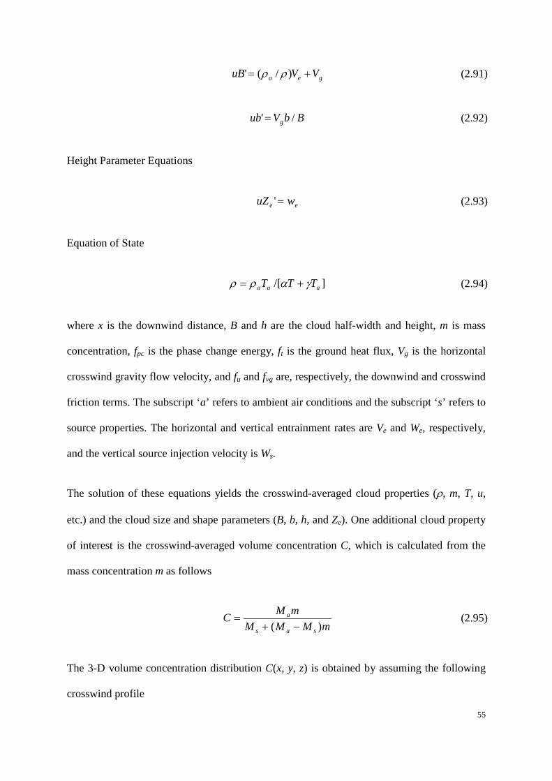
55

gea VVuB += )/(' ρρ (2.91)

BbVub g /' = (2.92)

Height Parameter Equations

ee wuZ =' (2.93)

Equation of State

]/[ aaa TTT gαρρ += (2.94)

where x is the downwind distance, B and h are the cloud half-width and height, m is mass

concentration, fpc is the phase change energy, ft is the ground heat flux, Vg is the horizontal

crosswind gravity flow velocity, and fu and fvg are, respectively, the downwind and crosswind

friction terms. The subscript ‘a’ refers to ambient air conditions and the subscript ‘s’ refers to

source properties. The horizontal and vertical entrainment rates are Ve and We, respectively,

and the vertical source injection velocity is Ws.

The solution of these equations yields the crosswind-averaged cloud properties (ρ, m, T, u,

etc.) and the cloud size and shape parameters (B, b, h, and Ze). One additional cloud property

of interest is the crosswind-averaged volume concentration C, which is calculated from the

mass concentration m as follows

mMMM

mMCsas

a

)( −+= (2.95)

The 3-D volume concentration distribution C(x, y, z) is obtained by assuming the following

crosswind profile

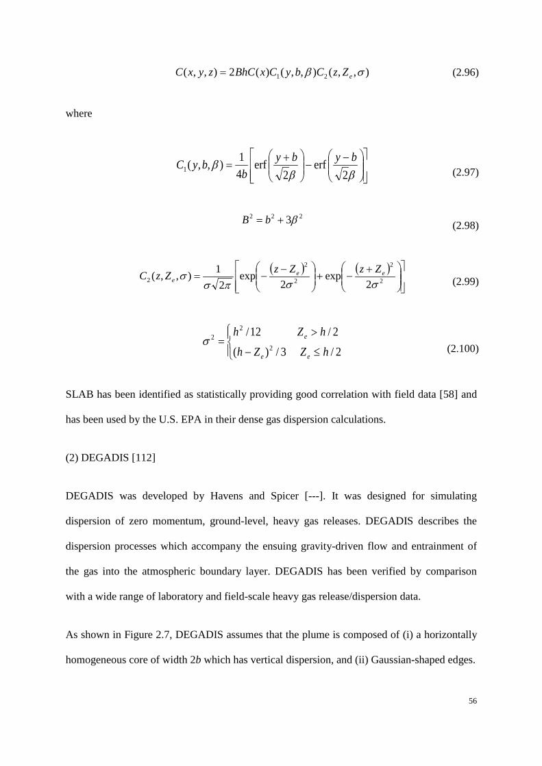
56

),,(),,()(2),,( 21 sβ eZzCbyCxBhCzyxC = (2.96)

where

−−

+=

βββ

2erf

2erf

41),,(1

bybyb

byC (2.97)

222 3β+= bB (2.98)

( ) ( )

+−+

−−= 2

2

2

2

2 2exp

2exp

21),,(

sspss ee

eZzZzZzC (2.99)

≤−

>=

2/3/)(

2/12/2

22

hZZhhZh

ee

es (2.100)

SLAB has been identified as statistically providing good correlation with field data [58] and

has been used by the U.S. EPA in their dense gas dispersion calculations.

(2) DEGADIS [112]

DEGADIS was developed by Havens and Spicer [---]. It was designed for simulating

dispersion of zero momentum, ground-level, heavy gas releases. DEGADIS describes the

dispersion processes which accompany the ensuing gravity-driven flow and entrainment of

the gas into the atmospheric boundary layer. DEGADIS has been verified by comparison

with a wide range of laboratory and field-scale heavy gas release/dispersion data.

As shown in Figure 2.7, DEGADIS assumes that the plume is composed of (i) a horizontally

homogeneous core of width 2b which has vertical dispersion, and (ii) Gaussian-shaped edges.

57

≤

−

>

−

−−

=+

+

)(exp)(

)()(

)(exp)(

),,(1

12

xbySzxC

xbySz

xSxby

xC

zyxCn

zc

n

zyc

(2.101)

where Cc(x) is the centreline ground-level concentration, Sy(x) the lateral dispersion

parameter, Sz(x) the vertical dispersion parameter, and b the half-width of the homogeneous

core section.

Figure 2.7 DEGADIS model - schematic

(3) Unified Dispersion Model (UDM) [113]

The Unified Dispersion Model (UDM) is the dispersion simulation module in the Phast

software package. UDM is an advanced similarity model capable of describing a wide range

of types of accidental releases. The main characteristic of similarity models is that profiles for

concentration, velocity, and temperature are assumed.

For a steady-state release, the continuous release profile is assumed to extend from the source

58

downwind. An elevated, heavy vapour/aerosol release starts out with a circular cross section.

Upon touching down, the cross section becomes a truncated ellipse, and the cloud levels off

as the vertical component of momentum is converted into downwind and cross-wind

momentum. The Cartesian co-ordinates x, y, z correspond to the downwind, cross-wind

(lateral horizontal) and vertical directions, respectively; x=0 corresponds to the point of

release, y=0 to the plume centre-line and z=0 to ground-level. In addition to these Cartesian

co-ordinates use is made of the ‘cloud’ coordinates s and ζ. Here, s is the arc length measured

along the plume centre, with s=0 corresponding to the point of release.

The concentration profile is given by

)()()(),,( 0 yFFxCyxC hv ζζ = (2.102)

−=)(

)(exp)(

xn

zv xR

F ζζ (2.103)

−=)(

)(exp)(

xm

yh xR

yyF (2.104)

The scaling coefficients in the above equations are:

yyR s2= (2.105)

zzR s2= (2.106)

When m=n=2, Eqs. 2.104 and 2.105 reduce to the Gaussian form, and sy and sz reduce to the

standard deviations (Gaussian vertical and cross-wind dispersion parameters).

59

Figure 2.8 UDM plume geometry for continuous release - schematic

Prior to Phast version 6.0, UDM adopted different sub-models for each subsequent phase for

a pressurised continuous release:(1) near-field jet model with uniform concentration profile,

(2) Gaussian jet model, (3) hybrid model [uniform profile, slumping], (4) dense-gas ground-

level dispersion, (5) far-field Gaussian passive dispersion. From version 6.0 onwards, a new

UDM model was introduced, which eliminates the problems associated with interfacing each

of the models and discontinuities between the models. The new UDM simplifies and

generalises the features of the models. It adopts a uniform concentration profile and seamless

transitions. Also, it adds new features in the areas of droplet evaporation, rainout, plume lift-

off and time-varying dispersion.

2.6.3 CFD dispersion model

In the past two decades, Computational Fluid Dynamics (CFD) simulation has been widely

used as an analysis methodology for pollutant dispersion. Topographic and atmospheric

conditions will significantly affect the atmospheric dispersion of CO2. In these conditions,

CFD generally performs better than other models because it allows the simulation of complex

60

physical processes involving heat and mass transport in complicated computational domains

[114]. In addition, CFD can provide detailed information about the concentration variables

and relevant flow throughout all computation domains. Though CFD is more time-consuming,

larger servers can offset part of this shortcoming.

Riddle et al. [115] investigated the suitability of using CFD (Fluent CFD code) to simulate

gas dispersion in the case of geometrically complex situations, such with buildings in close

proximity. The CFD results were compared with the prediction from the Atmospheric

Dispersion Modelling System (ADMS), a well-tested and validated quasi-Gaussian method.

Fluent was set up to simulate the neutrally stable atmospheric boundary layer. The mean

velocity profiles were well predicted and maintained downstream. The algebraic Reynolds

Stress turbulence model provided the best predictions for the turbulence kinetic energy (TKE)

and eddy dissipation rate. The dissipation rate was maintained throughout the computational

domain and, on average, the TKE levels were within 80% of the expected values up to a

height of 100 m, but at the ground, reduced to 50% of the inlet values. Prediction of TKE

using the standard k-ε turbulence model was much poorer. Spread of the gas plume was

predicted using an Advection-Diffusion (AD) method, a Lagrangian Particle tracking (LP)

method and a Large Eddy Simulation (LES) method. The LP method gave the best results:

the horizontal and vertical plumes were similar to those predicted by ADMS; the ground level

and plume centreline concentrations were close to ADMS values. However, some differences

were observed in the ground level concentrations which rise more rapidly with distance than

that predicted by ADMS, but reach similar peak values, while the plume centreline

concentrations dropped more rapidly than that predicted by ADMS. The CFD simulations

with the LP method produced satisfactory results, but should be tested further under different

atmospheric stability conditions. It was noted that CFD model is more appropriate in complex

situations (terrain, obstacles, etc).

61

Labovsky et al. [116] proposed a model for ammonia dispersion using fluent and simulated

the FLADIS field experiments. The released liquid phase was modelled as droplets using

discrete particle modelling, and the Euler-Lagrangian approach was applied for continuous

and discrete phases (air and ammonia vapour). It is found that the simulation results are

affected by the boundary conditions.

Leuning et al. [117] described various techniques for measuring CO2 emissions to the

atmosphere from geologically stored CO2, from point, line and area sources at scales of

metres to several kilometres. It was noted that the Flux Chamber technique was suitable for

measuring small leakage rates from sources at known locations but many samples were

required because of large spatial heterogeneity in the fluxes. Micrometeorological eddy

covariance, relaxed by eddy accumulation and flux gradient techniques were found suitable

for measuring leakage from large area sources, while integrated horizontal mass balance,

tracer methods and plume dispersion approaches were applicable to line and point sources.

The difficulty of distinguishing between leakage signals and natural fluctuations in CO2

concentrations due to bionic sources was noted. Forward Lagrangian dispersion calculations

showed that CO2 concentrations 0 – 80 m downwind of a point source would be readily

detectable above all natural variations for point sources > 0.3 gs-1 (about 10 tonnes CO2 per

year). An optimum monitoring strategy for inverse analysis (solving for the unknown

emission rate from measured wind fields and downwind concentration perturbations) would

require continuous measurements of CO2 and tracer compounds upwind and downwind of the

possible leak location, coupled with transport modelling to determine leakage fluxes, and to

differentiate them from other sources. Computations using The Air Pollution Model (TAPM)

showed that the expected perturbations in CO2 concentrations at distances of several hundred

meters from a leak of 32 gs-1 (about 1000 tonnes CO2 per year, or about 0.01% per year of a

typical amount to be stored) will be detectable, but this anomaly will be very small compared

62

to natural variations, thereby complicating the analysis. It was noted that none of these

techniques has yet been demonstrated for geo-sequestration.

Tauseef et al. [118] used CFD to simulate the CO2 dispersion in the presence of obstacles and

compared different turbulence models, recognized that the most commonly used models for

atmospheric dispersion of heavy gases – SLAB, HEGADAS, DEGADIS, HGSYSEM,

PHAST, SCIPUFF, TRACE, etc. The heavy gas assigned to a cylindrical volume is a Freon-

12/nitrogen mixture as in the experiments conducted earlier by the Health and Safety

Executive (HSE), UK, at Thorney Island, USA. The importance of the appropriate turbulence

model was recognized. Out of the various experiments done at that time, the findings of Trial

26 were used to identify the most appropriate turbulence model. It was found that the

realizable k-ε model is the most apt and enabled the closest prediction of the actual findings

in terms of spatial and temporal concentration profiles. It also can capture the phenomenon of

gravity slumping associated with heavy gas dispersion, while it also proved to be competitive

in terms of computing time required.

Michal et al. [119] proposed a model for two-phase dispersion of ammonia. The dispersion of

ammonia was modelled using a full set of numerically solved conservation equations with

additional equations for turbulence and a discrete particle model for liquid particle droplets.

Mazzoldi et al. [21] compared the simulations of CO2 dispersion by two classes of

atmospheric dispersion models (Gaussian modeland CFD model). The CFD model was used

to simulate a high-speed release with specified velocities with the aim of evaluating the effect

of initial gas dispersion on the downwind length reached by toxic concentrations of the

pollutant. Results showed a lowering of the risk involved in the transportation of CO2 by up

to one order of magnitude, when modelling the same releases with a CFD tool, compared to

the more widely used Gaussian models. The EU used results from Gaussian modelling for

63

drawing up an Impact Assessment on the CO2 transportation within CCS. Suggestions for

future preparation of CCS Risk Assessments were presented.

Pattison et al. [120, 121] proposed an integral model for two-phase release. The liquefied gas

was stored in a high pressure container and released. They considered the effects of cross-

flow, elevated jet, ground-level cloud, initial momentum, and dense cloud.

Pontiggia et al. [122] presented a new method for modelling the consequences of gas (SO2)

released under conditions of stable and neutral atmospheric stratification, and also considered

the obstacles. The approach was termed ASsM (Atmospheric Stability sub-Model), and was

used as an add-on user-defined feature to the CFD code. This involved adding a source term

to the ε conservation equation in the k-ε turbulence model, providing ground wall-type

boundary characterization and inlet boundary profiles in agreement with the Monin-Obukhov

similarity theory. The approach was validated via comparison with several field tests on the

Prairie Grass series, involving neutral, stable, and very stable stratification conditions.

Hulsbosch-Dam et al. [123] carried out a steady-state CFD model study of two-phase CO2

dispersion in a neutral atmosphere. The fluid state at the source was specified as either gas or

gas-solid with different solid mass fractions. CO2 concentrations at progressively larger

distances from the source were deduced. It was found that the gas-solid mixture with the

highest solid mass fraction at the source leads to the solid particles descending to the ground

and sublimating subsequently, leading to a higher CO2 concentration at relatively short

distances from the source.

Scargiali et al. [124] simulated the dispersion of heavy gas (chlorine) clouds over a large

topographically complex area (30 x 30 km2) by a general purpose CFD code. Due to the lager

simulation area and duration, large mesh (> = 1 m3) and time step (0.1 min) are chosen.

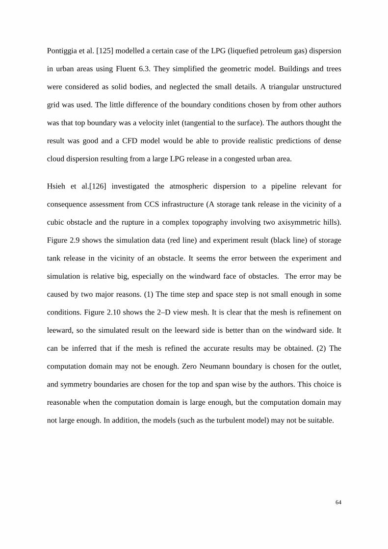
64

Pontiggia et al. [125] modelled a certain case of the LPG (liquefied petroleum gas) dispersion

in urban areas using Fluent 6.3. They simplified the geometric model. Buildings and trees

were considered as solid bodies, and neglected the small details. A triangular unstructured

grid was used. The little difference of the boundary conditions chosen by from other authors

was that top boundary was a velocity inlet (tangential to the surface). The authors thought the

result was good and a CFD model would be able to provide realistic predictions of dense

cloud dispersion resulting from a large LPG release in a congested urban area.

Hsieh et al.[126] investigated the atmospheric dispersion to a pipeline relevant for

consequence assessment from CCS infrastructure (A storage tank release in the vicinity of a

cubic obstacle and the rupture in a complex topography involving two axisymmetric hills).

Figure 2.9 shows the simulation data (red line) and experiment result (black line) of storage

tank release in the vicinity of an obstacle. It seems the error between the experiment and

simulation is relative big, especially on the windward face of obstacles. The error may be

caused by two major reasons. (1) The time step and space step is not small enough in some

conditions. Figure 2.10 shows the 2–D view mesh. It is clear that the mesh is refinement on

leeward, so the simulated result on the leeward side is better than on the windward side. It

can be inferred that if the mesh is refined the accurate results may be obtained. (2) The

computation domain may not be enough. Zero Neumann boundary is chosen for the outlet,

and symmetry boundaries are chosen for the top and span wise by the authors. This choice is

reasonable when the computation domain is large enough, but the computation domain may

not large enough. In addition, the models (such as the turbulent model) may not be suitable.

65

Figure 2.9 Time history of gas concentration on windward face of the obstacle at height of

6.4 m (top plan) and on leeward face of obstacle at height of 0.4 m (bottom plan)

Figure 2.10 The mesh in central line

Scargiali et al [127] simulated the dense cloud dispersion in urban areas using CFX. The

buildings were mimicked as distributed blocks and the buildings’ height, width, and face to

face distance were varied. Results showed that the presence of buildings lowered the

concentration maxima and enlarged the side spread of the cloud. The wind velocity had little

effect on the maximum concentrations at ground level.

Mocellin et al. [128] simulated the accident release of CO2 from CCS pipelines and the

66

consequences related to sublimating dry ice bank that may occur. Results showed that serious

risks were associated with the sublimating dry ice bank near the release point and the hazards

increased with a decreasing mean wind speed and a rise in ambient temperature.

2.7 Knowledge gaps

The literature review indicates that there still exist some knowledge gaps in the CO2

decompression and dispersion area. Firstly, in terms of CO2 or CO2 mixture decompression,

HRM multi-phase models is in its early stages, , which may be relative to the delayed

nucleation phenomenon in the decompression of CO2 pipelines. For CO2 dispersion,

generally speaking, the research associated with CO2 dispersion over complex terrains is in

its early stages. To quantify the risks associated with CO2 pipelines, an appropriate dispersion

model which can account for dispersion over complex terrains is essential.

2.8 Summary

This chapter presented the current available knowledge concerning the decompression,

expansion and dispersion behaviour of CO2 released from a high pressure pipeline. The

development of CO2 pipelines for CCS raises new questions regarding the control of ductile

fracture propagation and dispersion modelling. The literature review revealed that there were

still lots of knowledge gaps regarding this process.

More experimental and theoretical investigations of CO2 pipeline decompression are required.

However, experiments are usually very expensive and can only be used to investigate limited

factors. Therefore, theoretical prediction (i.e. using the CFD approach) is a valuable option in

order to improve our knowledge. Although in most cases of CO2 decompression, multi-phase

flow is involved, it is clear that the multi-phase CO2 decompression model is not well

investigated, probably because the simulation of phase change of CO2 during decompression

67

is very complicated. Also, compared with the measurements, the previous HEM models tend

to over-predict the pressure plateau in the decompression wave speed curve. Non-equilibrium

phase transition has been studied by some researchers, but there are still a host of limitations

for these HRMs as described in Section 2.2.2. Moreover, anthropogenic CO2 will contain

impurities that can modify the fluid decompression characteristics quite significantly; it is

therefore important for the modelling tools to handle CCS CO2 mixtures efficiently. However,

there has still not been any study for non-equilibrium effects on CO2 mixture decompression

to date.

The literature review shows that the presence of an obstacle and/or complex terrain has a

significant influence on heavy gas dispersion. Generally speaking, the research associated

with CO2 dispersion over complex terrains is in its early stages, and lots of deviations still

exist between simulated and measured results. Also, some technical details need to be

improved.

68

Chapter 3 Multi-phase decompression modelling of pure CO2

considering non-equilibrium phase transfer

69

Nomenclature

A cross-sectional area c speed of shound C mass transfer coefficient cp specific heat H enthalpy h latent heat

ID pipe internal diameter M mass transfer rate P pressure S source term/entropy T temperature t time u velocity V specific molar volume

vdr,p drift velocity W decompression wave speed x location

xeq equilibrium vapour quality Subscripts

0 initial condition ave average c critical e exit l liquid

local local m mixture/mass-averaged p pipe

s/sat saturation v vapour

3.1 Introduction

Fracture propagation is one of the key issues for the design and operation of pipelines and the

need to arrest a running fracture in a pipeline is paramount to the safety of a pipeline’s

operation. Because of the tendency of phase change and particular nature, previous studies

70

show that pipelines transporting CO2 will be more susceptible to running-ductile fracture than

one carrying natural gas [22]. As described in Chapter 1, accurate prediction of the

decompression wave is critical to study the fracture propagation. In addition, as part of the

safety assessment, the hazards associated with accidental CO2 pipeline failure must be

quantified and appropriate mitigating steps must be taken to bring their consequences to

acceptable levels [79]. Accordingly obtaining the parameters at the rupture plane including

the outflow rate, pressure, temperature and fractions of each fluid phase plays an essential

role. Such data can also be treated as the inputs for predicting the subsequent CO2

atmospheric expansion and dispersion. Thus, accurate pipe flow model after rupture is crucial

to the risk assessment of the CCS project.

After the initiation of a pipeline rupture, the pressure at the exit declines to choke pressure.

The residual pressure in the pipe will continue to drop below the saturation pressure.

Therefore in most rupture scenarios, the decompression path of fluid element inside the

pipeline would cross saturation line, resulting in a two-phase flow choked at the rupture plane.

Thus, an accurate prediction of the depressurisation inside the pipeline calls for the

development of engineering tools for the multi-phase CO2 flow.

In the last decades, several numerical models for the prediction of high-pressure pipe flow,

mainly in natural gas have been proposed, such as GASDECOM [129], DECOM [130],

EPDECOM [131]. These models use an analytical expression for the propagation of an

infinitesimal decompression front to determine the decompression wave speed without

explicitly solving the fluid transport equations. The main assumptions in such models include:

one-dimensional, frictionless, isentropic, and homogeneous equilibrium fluid flow. The main

difference between these models is the choice of EOS. Other more complex decompression

models that can account for non-isentropic conditions using Computational Fluid Dynamics

71

(CFD) techniques have also been developed, such as Picard and Bishnoi [55, 132], PipeTech

[133, 134] and CFD-DECOM [135]. They are also based on assumptions of one-dimensional

homogeneous equilibrium fluid flow.

Recently, CFD was increasingly employed to investigate multi-phase pipe flow [136-140].

As mentioned in Chapter 2, the majority of multi-phase decompression models in pipeline

studies reported in the literature have utilised HEM [141, 142], in which the constituent

phases were assumed to be in thermal and mechanical equilibrium throughout the phase

change process. Specifically, in HEM, the two phases share the same temperature and

pressure on the saturation line. Although results predicted by HEM were in reasonable

agreement with the measurements, there are still relatively great discrepancies between

simulation and measurements under some conditions. The predicted pressure plateaus in the

decompression wave speed curves were usually higher than those in the measured curves [18,

23]. It was suspected that the discrepancies were introduced by the thermal equilibrium

assumption in HEM [74]. Hence a flow model accounting for non-equilibrium phase

transition is desirable. Some researchers proposed to use a HRM [75, 76] which accounts for

the delay in vaporisation during the decompression process, and the delayed nucleation

probably affects the decompression characteristics of the fluid. Several numerical simulations

of the multi-phase flow using HRM have been reported, especially for Liquid Hydrogen (LH)

and water [94, 95, 98, 99]. However, the multi-phase CO2 decompression model is not well

investigated, probably because the simulation of phase change of CO2 during decompression

is much more complicated than that of water or LH. In a few recent publications, CO2

depressurisation or dispersion considering non-equilibrium phase transition has been

presented [78, 79, 102, 103]. However, as mentioned above, there are still a host of

limitations for these HRMs.

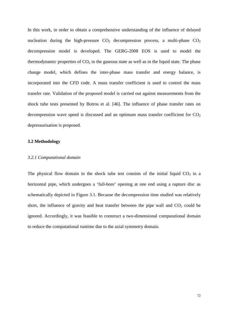
72

In this work, in order to obtain a comprehensive understanding of the influence of delayed

nucleation during the high-pressure CO2 decompression process, a multi-phase CO2

decompression model is developed. The GERG-2008 EOS is used to model the

thermodynamic properties of CO2 in the gaseous state as well as in the liquid state. The phase

change model, which defines the inter-phase mass transfer and energy balance, is

incorporated into the CFD code. A mass transfer coefficient is used to control the mass

transfer rate. Validation of the proposed model is carried out against measurements from the

shock tube tests presented by Botros et al. [46]. The influence of phase transfer rates on

decompression wave speed is discussed and an optimum mass transfer coefficient for CO2

depressurisation is proposed.

3.2 Methodology

3.2.1 Computational domain

The physical flow domain in the shock tube test consists of the initial liquid CO2 in a

horizontal pipe, which undergoes a ‘full-bore’ opening at one end using a rupture disc as

schematically depicted in Figure 3.1. Because the decompression time studied was relatively

short, the influence of gravity and heat transfer between the pipe wall and CO2 could be

ignored. Accordingly, it was feasible to construct a two-dimensional computational domain

to reduce the computational runtime due to the axial symmetry domain.

73

Figure 3.1 The physical domain (the cylinder) and computational domain (blue rectangle) –

schematic

3.2.2 The mixture multi-phase model

The mixture multi-phase model solves the continuity, momentum and energy equations for

mixture, and the volume fraction equation for the secondary phase/phases. In the process of

the decompression simulation, the liquid occupies most of the pipe; therefore the liquid CO2

was set as the primary phase, and vapour as the secondary phase. The slip velocity between

phases was activated i.e. the two phases were not in mechanical equilibrium.

The continuity equation of the mixture is [143]:

( ) ( ) 0=⋅∇+

∂∂

mmm vt

ρρ (3.1)

where mv , ρl and ρv is the mass-averaged velocity, liquid phase density and vapour phase

density, respectively:

m

vvvlllm ρ

vραvραv += (3.2)

and ρm is the density of the mixture, αl and αv are the volume fractions of liquid and vapour

phases, respectively.

Outflow Full-bore opening

Axis of symmetry

Computational domain

x = 0

74

vvllm ραραρ +=

(3.3)

The volume fraction for the second phase can be obtained from the continuity equation for

each phase, as

( ) ( ) vpdrvvmvvvv Svv

t+⋅−∇=⋅∇+

∂∂ )( ,ραραρα

(3.4)

where Sv is the mass source term of the vapour

lvvlv mmS −− −= (3.5)

The mass source term of liquid is

vllvvl mmSS −− −=−= (3.6)

The source terms Sv and Sl represent the mass transfer rates between two phases.

The momentum equation of the mixture can be obtained by summing the individual

momentum equations for all phases as:

( ) ( ) ( )kdrkdrkknkm

Tmmmmmmmm vvFgvvpvvv

t,,1 ραρmρρ =∑+++

∇+∇⋅∇+−∇=⋅∇+

∂∂

(3.7)

where n is the number of phases, F is a body force, and mm is the viscosity of the mixture.

75

kdrv , is the drift velocity for secondary phase (vapour) as:

mkkdr vvv −=, (3.8)

The energy equation of the mixture takes the following form:

( ) ( )[ ] Eeffvvvvvvvlll STkpEvEEt

+∇⋅⋅∇=+⋅∇++∂∂ )(ραραρα (3.9)

where, keff is the effective conductivity, depending on the turbulence model used. SE includes

any other volumetric heat sources, which can be defined as an energy source term and

implemented in ANSYS Fluent.

3.2.3 Numerical Methods

The Finite-Volume Method is used in ANSYS Fluent to discretise the conservation equations.

Here the computational domain is divided into a number of sub-regions called ‘control

volumes’ or ‘cells’. The governing equations are integrated over all the control volumes of

the computational domain. The resulting integral equations are expressed like algebraic

equations which are solved numerically [144].

The pressure-based solver was chosen because it is compatible with the multi-phase sub-

model. The pressure-based solver employs an algorithm which belongs to a general class of

methods called the projection method [145]. In the projection method, the constraint of mass

conservation of the velocity field is achieved by solving a pressure (or pressure correction)

equation. The pressure equation is derived from the continuity and the momentum equations

in such way that the velocity field, corrected by the pressure, satisfied the continuity. Since

the governing equations are nonlinear and coupled to one another, the solution process

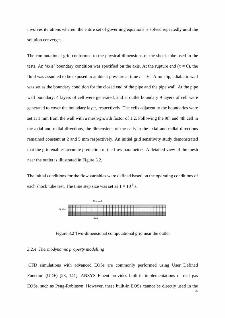
76

involves iterations wherein the entire set of governing equations is solved repeatedly until the

solution converges.

The computational grid conformed to the physical dimensions of the shock tube used in the

tests. An ‘axis’ boundary condition was specified on the axis. At the rupture end (x = 0), the

fluid was assumed to be exposed to ambient pressure at time t = 0s. A no-slip, adiabatic wall

was set as the boundary condition for the closed end of the pipe and the pipe wall. At the pipe

wall boundary, 4 layers of cell were generated, and at outlet boundary 9 layers of cell were

generated to cover the boundary layer, respectively. The cells adjacent to the boundaries were

set at 1 mm from the wall with a mesh-growth factor of 1.2. Following the 9th and 4th cell in

the axial and radial directions, the dimensions of the cells in the axial and radial directions

remained constant at 2 and 5 mm respectively. An initial grid sensitivity study demonstrated

that the grid enables accurate prediction of the flow parameters. A detailed view of the mesh

near the outlet is illustrated in Figure 3.2.

The initial conditions for the flow variables were defined based on the operating conditions of

each shock tube test. The time step size was set as 1 × 10-6 s.

Figure 3.2 Two-dimensional computational grid near the outlet

3.2.4 Thermodynamic property modelling

CFD simulations with advanced EOSs are commonly performed using User Defined

Function (UDF) [23, 141]. ANSYS Fluent provides built-in implementations of real gas

EOSs, such as Peng-Robinson. However, these built-in EOSs cannot be directly used in the

Pipe wall

Outlet

Axis

77

multi-phase model, as they do not explicitly separate properties for two phases. To solve this

problem, a User-Defined Real Gas Model (UDRGM) was introduced, which could be

implemented through UDFs [143]. In the UDRGM, physical properties of the fluid, such as

density, enthalpy, entropy, specific heat and speed of sound, can be solved at given pressure

and temperature at runtime using a real gas EOS. As the GERG-2008 EOS is accurate

sufficiently to describe the thermodynamic property for pure CO2 and CO2 mixtures, it was

employed in this work. A two-dimensional (2D) pressure-temperature (P-T) table was

established as a structured two-dimensional array for chosen ranges of pressure and

temperature. The GERG-2008 EOS library, was called for each P-T node in the 2D-table to

produce tables of the properties (Density ρ, Enthalpy h, Entropy s, Speed of sound c, Specific

heat at constant pressure cp, Molecular weight M, Partial derivative of ρ w.r.t. T ∂ρ / ∂T,

Partial derivative of ρ w.r.t. P ∂ρ / ∂P, Partial derivative of h w.r.t. P ∂h / ∂P) for liquid CO2.

UDF was also used to describe the thermodynamic properties of gaseous CO2 as a function of

temperature and pressure. The properties were also solved using GERG-2008 EOS. For the

gaseous phase, UDFs were built for density and speed of sound at each P-T node. Different

from the liquid phase, the influence of pressure on enthalpy (Hl) and heat capacity (Cpv) was

ignored due to the limitation of ANSYS Fluent in supporting real gas EOS for multi-phase

modelling. The enthalpy and heat capacity were fitted with temperature at the saturation line.

The entropy was calculated as

⋅=

refpvl T

TCS log (3.10)

where Tref is the reference temperature.

3.2.5 Source terms

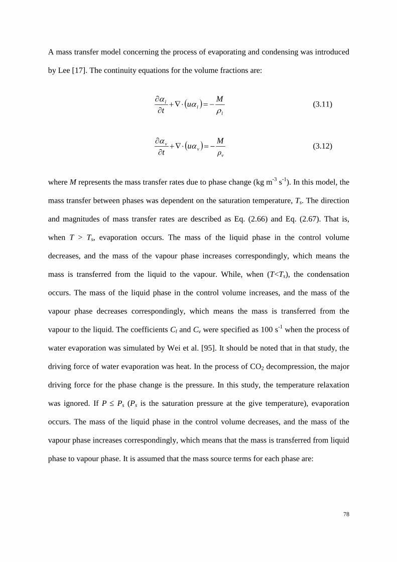
78

A mass transfer model concerning the process of evaporating and condensing was introduced

by Lee [17]. The continuity equations for the volume fractions are:

( )l

ll Mu

t ραα

−=⋅∇+∂

∂ (3.11)

( )v

vv

ρMu

t−=⋅∇+

∂∂ αα (3.12)

where M represents the mass transfer rates due to phase change (kg m-3 s-1). In this model, the

mass transfer between phases was dependent on the saturation temperature, Ts. The direction

and magnitudes of mass transfer rates are described as Eq. (2.66) and Eq. (2.67). That is,

when T > Ts, evaporation occurs. The mass of the liquid phase in the control volume

decreases, and the mass of the vapour phase increases correspondingly, which means the

mass is transferred from the liquid to the vapour. While, when (T<Ts), the condensation

occurs. The mass of the liquid phase in the control volume increases, and the mass of the

vapour phase decreases correspondingly, which means the mass is transferred from the

vapour to the liquid. The coefficients Cl and Cv were specified as 100 s-1 when the process of

water evaporation was simulated by Wei et al. [95]. It should be noted that in that study, the

driving force of water evaporation was heat. In the process of CO2 decompression, the major

driving force for the phase change is the pressure. In this study, the temperature relaxation

was ignored. If P ≤ Ps (Ps is the saturation pressure at the give temperature), evaporation

occurs. The mass of the liquid phase in the control volume decreases, and the mass of the

vapour phase increases correspondingly, which means that the mass is transferred from liquid

phase to vapour phase. It is assumed that the mass source terms for each phase are:

79

s

slllvl P

PPραCSS −=−= (3.13)

while, when P ≥ Ps

s

svvvvl p

PPραCSS −=−= (3.14)

As long as the mass source term is obtained, the energy source term can be obtained by

taking the latent heat during the phase change into account:

llvE ShS ⋅= (3.15)

where hlv is the latent heat at any given temperature, which can be calculated as

( )slvlv HHh −= (3.16)

where, Hv and Hl are the enthalpy of vapour and liquid in saturation condition, respectively.

3.3 Results and discussion

The shock tube test 32A conducted by Botros et al. at the TransCanada pipeline Gas Dynamic

test Facility in Didsbury, Alberta, Canada [69] was simulated using the proposed model for

validation. The shock tube consists of four spool pieces of NPS 2 stainless-steel pipe making

up a total length of 42 m. They are made of NPS 2 x 11.1 mm WT, SCH XX, ASTM A312,

316 SS seamless tube. All individual spools were designed for 41.370 MPa pressure, design

factor = 0.8 and location factor = 0.625 (according to the latest edition of the CSA Standard

Z662). ANSI 2500 RTJ flanges (PN 420 Standards) ASTM A182 - 316 SS were used. The

spool was shop-tested to a minimum hydrostatic pressure of 62.055 MPa, and a maximum

80

hydrostatic pressure of 62.755 MPa for a period of one hour. The initial pressure and

temperature were 11.27 MPa and 281.89 k, and pure CO2 was used.in the test. The diameter

of the tube was 38.1 mm. The tube was fitted with fluid and the rupture disc was at the front

end of the shock tube. At time of cutting of the rupture disc, the pipe was opened to the

atmosphere and a decompression wave propagated up the tube. The locations of pressure and

temperature transducers mounted on these tests are presented in Table 3-1.

Table 3-1 The locations of pressure transducers Table 3-1

Location Distance from rupture disc (m)

PT1 0.0295

PT1A 0.0924

PT1B 0.1028

PT2 0.2

PT3 0.35

PT4 0.5

PT5 0.7

PT6 0.9

PT7 1.1

PT8 3.1

PT9 5.1

PT10 7.1

PT11 9.1

In the CFD model, according to the locations where the pressure transducers and temperature

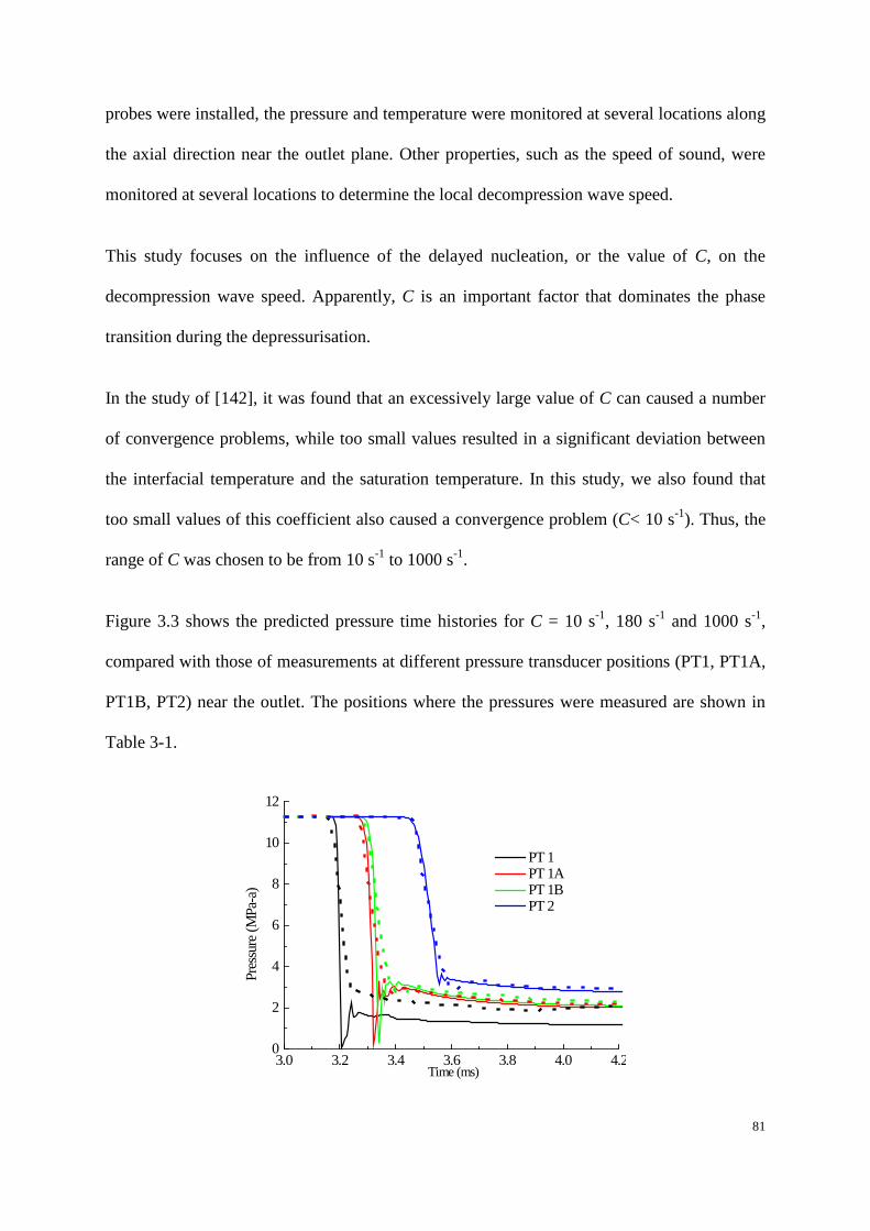
81

probes were installed, the pressure and temperature were monitored at several locations along

the axial direction near the outlet plane. Other properties, such as the speed of sound, were

monitored at several locations to determine the local decompression wave speed.

This study focuses on the influence of the delayed nucleation, or the value of C, on the

decompression wave speed. Apparently, C is an important factor that dominates the phase

transition during the depressurisation.

In the study of [142], it was found that an excessively large value of C can caused a number

of convergence problems, while too small values resulted in a significant deviation between

the interfacial temperature and the saturation temperature. In this study, we also found that

too small values of this coefficient also caused a convergence problem (C< 10 s-1). Thus, the

range of C was chosen to be from 10 s-1 to 1000 s-1.

Figure 3.3 shows the predicted pressure time histories for C = 10 s-1, 180 s-1 and 1000 s-1,

compared with those of measurements at different pressure transducer positions (PT1, PT1A,

PT1B, PT2) near the outlet. The positions where the pressures were measured are shown in

Table 3-1.

3.0 3.2 3.4 3.6 3.8 4.0 4.20

2

4

6

8

10

12

PT 1 PT 1A PT 1B PT 2

Pres

sure

(MPa

-a)

Time (ms)

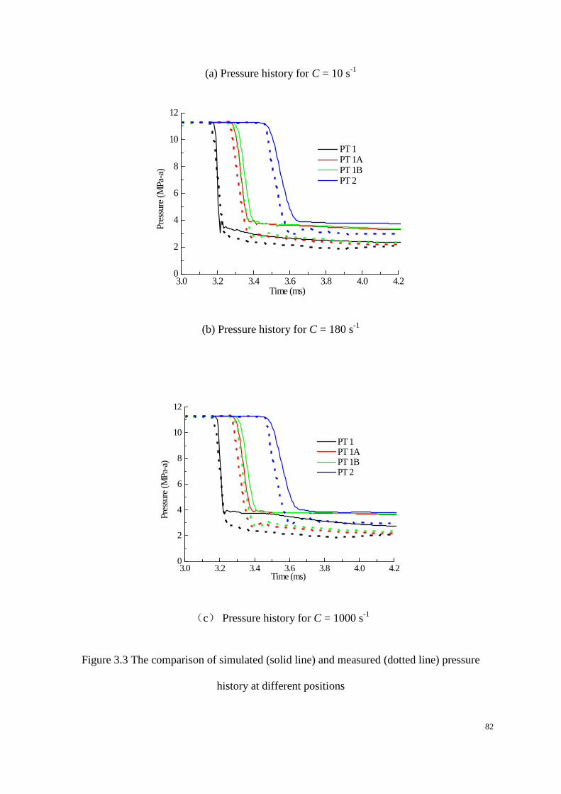
82

(a) Pressure history for C = 10 s-1

3.0 3.2 3.4 3.6 3.8 4.0 4.20

2

4

6

8

10

12

PT 1 PT 1A PT 1B PT 2

Pres

sure

(MPa

-a)

Time (ms)

(b) Pressure history for C = 180 s-1

3.0 3.2 3.4 3.6 3.8 4.0 4.20

2

4

6

8

10

12

PT 1 PT 1A PT 1B PT 2

Pres

sure

(MPa

-a)

Time (ms)

（c） Pressure history for C = 1000 s-1

Figure 3.3 The comparison of simulated (solid line) and measured (dotted line) pressure

history at different positions

83

The experimental results show that the pressure undergoes an initial sharp drop and then

remains at a relatively stable plateau, on which the pressure decreases gradually but slowly.

The trend of the pressure drop is successfully predicted by the model. There is also good

agreement between the predicted and measured pressure curves. It can be found that the

arrival of the decompression wave is significantly affected by the delayed nucleation at each

position. Specifically, the delayed nucleation results in earlier decompression. When using C

= 10 s-1, the arrival time of decompression is in best agreement with the measurements.

Additionally, the predicted pressure curve is closer to the measurements during the pressure

plateau when a smaller value of C is chosen. The predicted pressure is a little higher than the

measured pressure at the plateau when a larger value of C is chosen. Notice that the value of

C and the relaxation time factor t is in inverse relationship, therefore the results are in

accordance with the results obtained by Brown et al. [46], who pointed out that less pressure

drop was observed when the relaxation time decreased [78]. However, the pressure

fluctuation obtained by a smaller value of C is sharper before reaching the pressure plateau.

The observations highlight the necessity of accounting for the non-equilibrium effects during

depressurisation. Figure 3.4 presents the thermodynamic trajectory of the CO2 decompression

at positon PT2 for different values of C, relative to the CO2 saturation line. After the P-T path

crosses the saturation line, for a larger value of C, the pressure is closer to the saturation

pressure. When a smaller value of C is chosen, the pressure can be much lower than the

saturation pressure, leading to stronger delayed nucleation. Consequently, a smaller value of

C results in lower plateau pressure. In addition, the pressure fluctuation is caused by that

when the decompression passes the saturation line, the properties of liquid CO2 is assumed to

be equal to those on the saturation line. In fact, up to now, from author’s knowledge, there is

virtually no experimental data or EOSs about neither the exact liquid properties below the

saturation line or the vapour properties above the saturation line. This assumption may bring

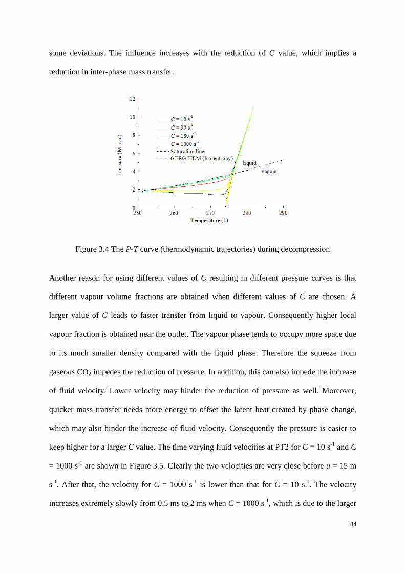
84

some deviations. The influence increases with the reduction of C value, which implies a

reduction in inter-phase mass transfer.

Figure 3.4 The P-T curve (thermodynamic trajectories) during decompression

Another reason for using different values of C resulting in different pressure curves is that

different vapour volume fractions are obtained when different values of C are chosen. A

larger value of C leads to faster transfer from liquid to vapour. Consequently higher local

vapour fraction is obtained near the outlet. The vapour phase tends to occupy more space due

to its much smaller density compared with the liquid phase. Therefore the squeeze from

gaseous CO2 impedes the reduction of pressure. In addition, this can also impede the increase

of fluid velocity. Lower velocity may hinder the reduction of pressure as well. Moreover,

quicker mass transfer needs more energy to offset the latent heat created by phase change,

which may also hinder the increase of fluid velocity. Consequently the pressure is easier to

keep higher for a larger C value. The time varying fluid velocities at PT2 for C = 10 s-1 and C

= 1000 s-1 are shown in Figure 3.5. Clearly the two velocities are very close before u = 15 m

s-1. After that, the velocity for C = 1000 s-1 is lower than that for C = 10 s-1. The velocity

increases extremely slowly from 0.5 ms to 2 ms when C = 1000 s-1, which is due to the larger

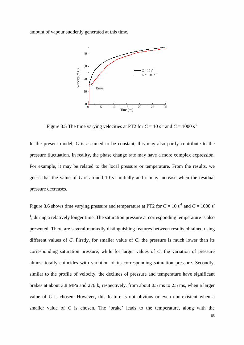
85

amount of vapour suddenly generated at this time.

0 5 10 15 20 25 300

10

20

30

40

Velo

city

(m s-1

)

Time (ms)

C = 10 s-1

C = 1000 s-1

Brake

Figure 3.5 The time varying velocities at PT2 for C = 10 s-1 and C = 1000 s-1

In the present model, C is assumed to be constant, this may also partly contribute to the

pressure fluctuation. In reality, the phase change rate may have a more complex expression.

For example, it may be related to the local pressure or temperature. From the results, we

guess that the value of C is around 10 s-1 initially and it may increase when the residual

pressure decreases.

Figure 3.6 shows time varying pressure and temperature at PT2 for C = 10 s-1 and C = 1000 s-

1, during a relatively longer time. The saturation pressure at corresponding temperature is also

presented. There are several markedly distinguishing features between results obtained using

different values of C. Firstly, for smaller value of C, the pressure is much lower than its

corresponding saturation pressure, while for larger values of C, the variation of pressure

almost totally coincides with variation of its corresponding saturation pressure. Secondly,

similar to the profile of velocity, the declines of pressure and temperature have significant

brakes at about 3.8 MPa and 276 k, respectively, from about 0.5 ms to 2.5 ms, when a larger

value of C is chosen. However, this feature is not obvious or even non-existent when a

smaller value of C is chosen. The ‘brake’ leads to the temperature, along with the

86

corresponding saturation pressure, being higher at this period for a larger value of C. The two

temperature paths diverge at about 0.3 ms, and the temperature will be higher for lager values

of C. Then the temperature paths converge at 4.02 ms, after that the temperature is lower for a

larger value of C, because a larger value of C, which means faster transfer rate from liquid to

vapour, costs more energy to offset the latent heat. Therefore, for a long-time, the

temperature will be lower. The saturation pressure, which depends on the temperature, shows

the same trend with that of temperature. Consequently, the saturation pressure is lower for

larger values of C than that for smaller values of C.

0 10 20 30

2

4

6

8

10

12

Brake

Pres

sure

(MPa

-a)

Time (ms)

C = 10 s-1, P C = 10 s-1, Ps

C = 1000 s-1, P C = 1000 s-1, Ps

Brake

255

260

265

270

275

280

285 C = 10 s-1, T C = 1000 s-1, T

Tem

pera

ture

(k)

Figure 3.6 The time varying pressure and temperature as well as the saturation pressure at

corresponding temperature at PT2

When a pipeline rupture occurs, a leading decompression wave propagates away from the

rupture plane into the undisturbed compressed fluid at the local speed of sound. Behind the

leading decompression wave, the local decompression wave velocity is equal to the local

speed of sound minus the local escaping out flow velocity. The decompression curve or more

precisely the decompression wave velocity vs pressure is an important factor for fracture

control analysis according to BTCM.

87

The speed of sound c and the outflow velocity u as a function of time were monitored to

obtain the local decompression wave speed during the decompression process. The

decompression wave speed was then determined by subtracting the outflow velocity from the

speed of sound for several pressures below the initial pressure. The local decompression

wave speed was determined using the predicted speed of sound and outflow velocity at 200

mm (PT2) from the outlet. However, experimental tests such as the shock tube test do not

provide the local decompression wave speed directly. The decompression wave speed W is

calculated by determining the times at which a certain pressure level is recorded at several

pressure transducers at known locations on the pipe wall. By plotting these locations against

time, the decompression wave speed can be obtained by performing a linear regression of

each isobar curve. The slope of each regression represents the average decompression wave

speed for each isobar.

The average decompression wave speed in the simulation is calculated using an approach

similar to that used in processing the measured data (based on the pressure-time traces). This

initial decompression wave speed was fitted using the data obtained by the first 6 points, as

shown in Figure 3.7.

88

0.0000 0.0002 0.0004 0.0006 0.00080.0

0.1

0.2

0.3

0.4

0.5

Dista

nce f

rom

the o

utle

t (m

)

Time (s)

Y = 591.26X + 0.0242

C = 10 s-1

Figure 3.7 Determination of the initial average decompression wave speed

0 100 200 300 400 500 6000

2

4

6

8

10

12

The measured start of the plateau

Experiment C = 10 s-1

C = 30 s-1

C = 180 s-1

C = 1000 s-1

GERG-HEM

Pres

sure

(MPa

-a)

Decompression wave speed (m s-1)

Plateau

Rapiddecreaseperiod

The start of the plateau for GERG-HEM

Figure 3.8 Comparison of the measured and simulated decompression wave speeds using

different values of C as well as using GERG-HEM

Figure 3.8 compares the measured and simulated average decompression wave speeds (Wave)

using different values of C. Each decompression wave speed vs pressure curve is able to be

divided into two periods. One is the rapid drop period when the residual pressure is relatively

high and the other is the relatively stable plateau after phase change occurs. For a larger value

of C, the Wave is lower than that measured in the rapid drop period. This is because as

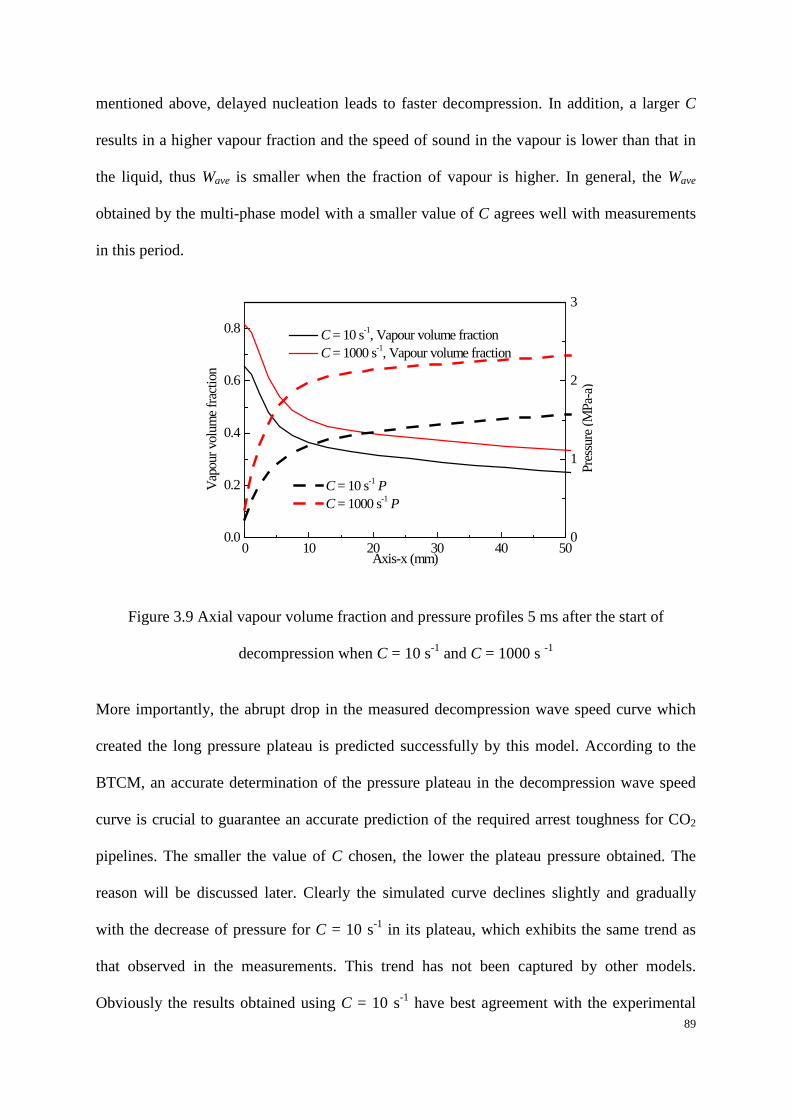
89

mentioned above, delayed nucleation leads to faster decompression. In addition, a larger C

results in a higher vapour fraction and the speed of sound in the vapour is lower than that in

the liquid, thus Wave is smaller when the fraction of vapour is higher. In general, the Wave

obtained by the multi-phase model with a smaller value of C agrees well with measurements

in this period.

0 10 20 30 40 500.0

0.2

0.4

0.6

0.8

Vapo

ur v

olum

e fra

ction

Axis-x (mm)

C = 10 s-1, Vapour volume fraction C = 1000 s-1, Vapour volume fraction

0

1

2

3

C = 10 s-1 P C = 1000 s-1 P

Pres

sure

(MPa

-a)

Figure 3.9 Axial vapour volume fraction and pressure profiles 5 ms after the start of

decompression when C = 10 s-1 and C = 1000 s -1

More importantly, the abrupt drop in the measured decompression wave speed curve which

created the long pressure plateau is predicted successfully by this model. According to the

BTCM, an accurate determination of the pressure plateau in the decompression wave speed

curve is crucial to guarantee an accurate prediction of the required arrest toughness for CO2

pipelines. The smaller the value of C chosen, the lower the plateau pressure obtained. The

reason will be discussed later. Clearly the simulated curve declines slightly and gradually

with the decrease of pressure for C = 10 s-1 in its plateau, which exhibits the same trend as

that observed in the measurements. This trend has not been captured by other models.

Obviously the results obtained using C = 10 s-1 have best agreement with the experimental

90

data in both the plateau and rapid pressure drop periods.

The comparison of the local decompression wave speed (Wlocal) using HEM with GERG-

2008 EOS (called GERG-HEM) obtained by Botros et al. [46] and the average

decompression wave speed using our CFD multi-phase model is also shown in Figure 3.8.

Notice that the results obtained from experimental data and the simulation are the average

decompression wave speed, whereas those obtained by GERG-HEM are the local

decompression speed. In general both GERG-HEM and the multi-phase model using C = 10

s-1 predicted the decompression wave speed well before the curves reach the plateau. As the

pressure decreases, the predicted decompression wave speed obviously differs from the two

models. Compared to the experimental results, GERG-HEM over-predicted the

decompression wave speed in this period. This may be partly due to an under-prediction of

velocity, which will be discussed later. The pressure predicted using GERG-HEM arrives at

the plateau earlier than that obtained from measurement, whereas the predicted and measured

pressures reach the plateau nearly at the same pressure, when the proposed multi-phase model

with C = 10 s-1 is used. This comes from the fact that the pressure predicted by HEM is not

able to cross the saturation line but that predicted by the proposed multi-phase model is able

to, as shown in Figure 3.4. The positions of the front end of the plateau in HEM predictions

deviate from the measured. This is due to the time duration in the rapid decrease period being

much shorter than that measured for HEM. Consequently, HEM over-predicts the plateau

pressure significantly. However, the proposed multi-phase model predicted a plateau pressure

in quite good agreement with the measurements. It can also be seen that if a larger value of C

is chosen, a plateau pressure closer to that obtained by GERG-HEM will be predicted. In the

multi-phase model, a larger value of C results in a faster transfer rate from liquid to vapour,

leading to higher vapour fraction. As the speed of sound of vapour is far smaller than that of

liquid, a larger value of C leads to lower sound speed in the mixture. It can also be found that

91

the gaps in pressure plateau between simulations are very small when C >= 180 s-1. Clearly,

like the pressure predicted by the GERG-HEM model, larger values of C over-predict the

plateau level as well. This proves that delayed nucleation during phase change does impact

the decompression wave speed. The decompression curve in the plateau in the experimental

results shows a decreasing trend with the reduction of pressure. This trend was not captured

by the GERG-HEM model, but it can be predicted by the proposed multi-phase model.

The results of local decompression wave speed (Wlocal) using C=10 s-1, 180 s-1 and 1000 s-1

are compared with those obtained by GERG-HEM in Figure 3.10. Initially there is nearly no

difference but the curve is a little lower at the plateau when a smaller value of C is chosen.

The decline trend predicted by the multi-phase model is discernible. Notice that the

experimental data is Wave, and in fact part of the deviation is caused by the Wlocal not being

equal to Wave under some conditions. The data processing methodology may affect the results

of decompression wave speed because the decompression wave speed may be influenced by

the position. Clearly Wlocal shows the same decreasing trend with Wave, but a little lower than

Wave. In the multi-phase model, the mass gradually transfers between phases. The speed of

sound of vapour is much lower than that of liquid. The local speed of sound of the mixture

will gradually decrease with the gradually increasing vapour fraction. Therefore the curve of

decompression wave speed vs pressure presents a decline trend on the plateau.

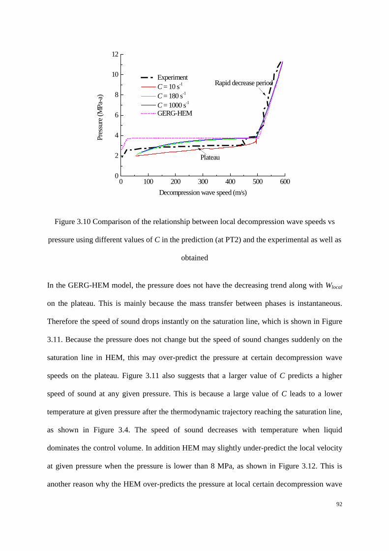
92

0 100 200 300 400 500 6000

2

4

6

8

10

12

Experiment C = 10 s-1

C = 180 s-1

C = 1000 s-1

GERG-HEM

Pres

sure

(MPa

-a)

Decompression wave speed (m/s)

Plateau

Rapid decrease period

Figure 3.10 Comparison of the relationship between local decompression wave speeds vs

pressure using different values of C in the prediction (at PT2) and the experimental as well as

obtained

In the GERG-HEM model, the pressure does not have the decreasing trend along with Wlocal

on the plateau. This is mainly because the mass transfer between phases is instantaneous.

Therefore the speed of sound drops instantly on the saturation line, which is shown in Figure

3.11. Because the pressure does not change but the speed of sound changes suddenly on the

saturation line in HEM, this may over-predict the pressure at certain decompression wave

speeds on the plateau. Figure 3.11 also suggests that a larger value of C predicts a higher

speed of sound at any given pressure. This is because a large value of C leads to a lower

temperature at given pressure after the thermodynamic trajectory reaching the saturation line,

as shown in Figure 3.4. The speed of sound decreases with temperature when liquid

dominates the control volume. In addition HEM may slightly under-predict the local velocity

at given pressure when the pressure is lower than 8 MPa, as shown in Figure 3.12. This is

another reason why the HEM over-predicts the pressure at local certain decompression wave

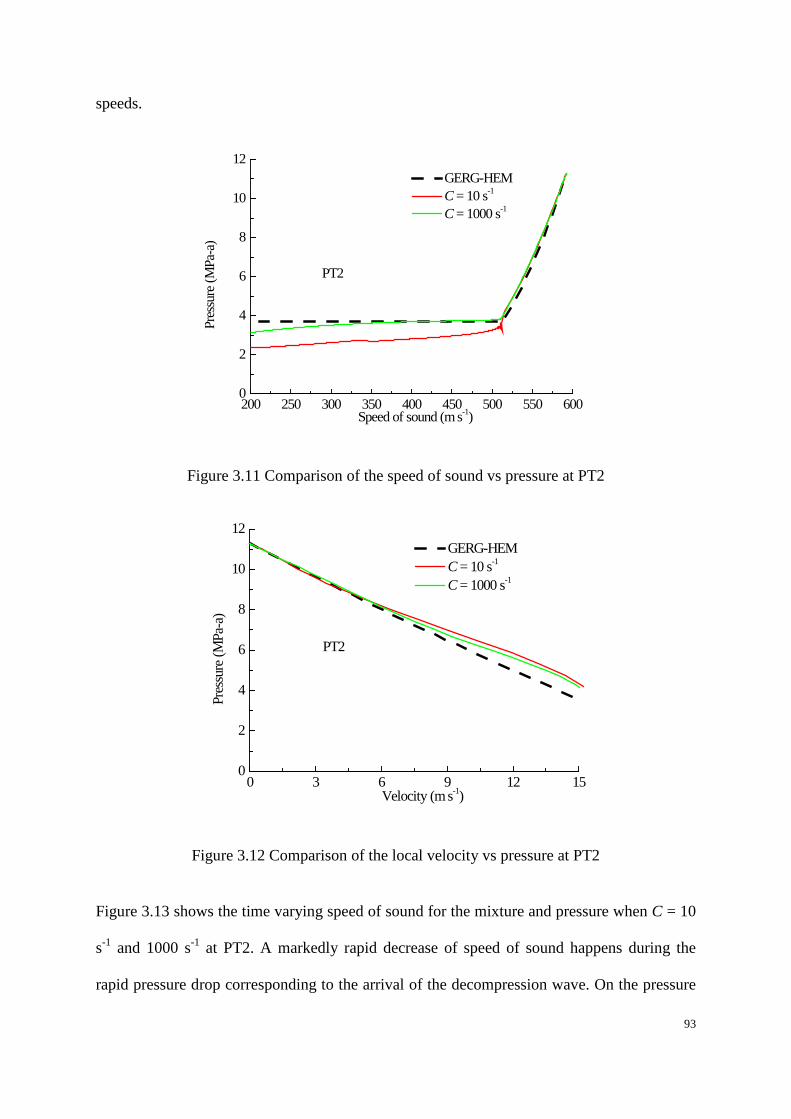
93

speeds.

200 250 300 350 400 450 500 550 6000

2

4

6

8

10

12

Pres

sure

(MPa

-a)

Speed of sound (m s-1)

GERG-HEM C = 10 s-1

C = 1000 s-1

PT2

Figure 3.11 Comparison of the speed of sound vs pressure at PT2

0 3 6 9 12 150

2

4

6

8

10

12

Pres

sure

(MPa

-a)

Velocity (m s-1)

GERG-HEM C = 10 s-1

C = 1000 s-1

PT2

Figure 3.12 Comparison of the local velocity vs pressure at PT2

Figure 3.13 shows the time varying speed of sound for the mixture and pressure when C = 10

s-1 and 1000 s-1 at PT2. A markedly rapid decrease of speed of sound happens during the

rapid pressure drop corresponding to the arrival of the decompression wave. On the pressure

94

plateau, the speed of sound still declines rapidly when C = 10 s-1, whereas it remains at about

540 m s-1 for about 2 ms. The smaller value of C makes the lower speed of sound.

Consequently this makes the local decompression wave speed lower.

0.0 0.5 1.0 1.5 2.0 2.5 3.0200

250

300

350

400

450

500

550

600

C = 10 s-1, P C = 1000 s-1, P C = 10 s-1, Speed of sound C = 1000 s-1, Speed of sound

Time (ms)

Spee

d of

Sou

nd (m

s-1)

0

2

4

6

8

10

12

Pres

sure

(MPa

-a)

Figure 3.13 The speed of sound and pressure as a function of time using different values of C

To further elucidate the effect of C on phase change behaviour during the decompression,

Figure 3.4 is discussed here. The thermodynamic trajectory can cross the saturation line is the

distinguishing feature of the multi-phase model, which will influence a host of characters. In

addition, the iso-entropy path using GERG-HEM is also shown in Figure 3.4. It can be seen

that the paths show serval distinct trends relative to the phase boundary, which include:

(1) The thermodynamic trajectories obtained by various C as well as iso-entropy path

obtained using GERG-HEM are very close before reaching the saturation line. In this

period, the phase change doesn’t happen in the control volume. Therefore the

reduction of the temperature is due to the Joules-Thomson effect [148]. Consequently

the value of C has nearly no influence on the thermodynamic trajectory. In this period,

a pressure drop of more than 10 MPa from initial state to the saturation line is

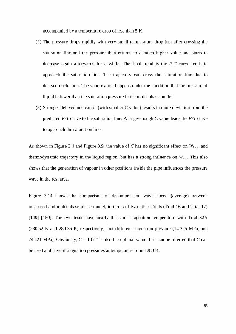
95

accompanied by a temperature drop of less than 5 K.

(2) The pressure drops rapidly with very small temperature drop just after crossing the

saturation line and the pressure then returns to a much higher value and starts to

decrease again afterwards for a while. The final trend is the P-T curve tends to

approach the saturation line. The trajectory can cross the saturation line due to

delayed nucleation. The vaporisation happens under the condition that the pressure of

liquid is lower than the saturation pressure in the multi-phase model.

(3) Stronger delayed nucleation (with smaller C value) results in more deviation from the

predicted P-T curve to the saturation line. A large-enough C value leads the P-T curve

to approach the saturation line.

As shown in Figure 3.4 and Figure 3.9, the value of C has no significant effect on Wlocal and

thermodynamic trajectory in the liquid region, but has a strong influence on Wave. This also

shows that the generation of vapour in other positions inside the pipe influences the pressure

wave in the rest area.

Figure 3.14 shows the comparison of decompression wave speed (average) between

measured and multi-phase phase model, in terms of two other Trials (Trial 16 and Trial 17)

[149] [150]. The two trials have nearly the same stagnation temperature with Trial 32A

(280.52 K and 280.36 K, respectively), but different stagnation pressure (14.225 MPa, and

24.421 MPa). Obviously, C = 10 s-1 is also the optimal value. It is can be inferred that C can

be used at different stagnation pressures at temperature round 280 K.

96

(a) Decompression wave in Trial 16

(b) Decompression wave in Trial 17

Figure 3.14 Decompression wave speed (average) between measured and multi-phase phase

model, in terms of other two Trials (Trial 16 and Trial 17)

In the study of [151], Munkejord et al proposed a model for calculating the transport and

depressurization of a CO2-CH4 mixture. The model accounted for phase slip though drift

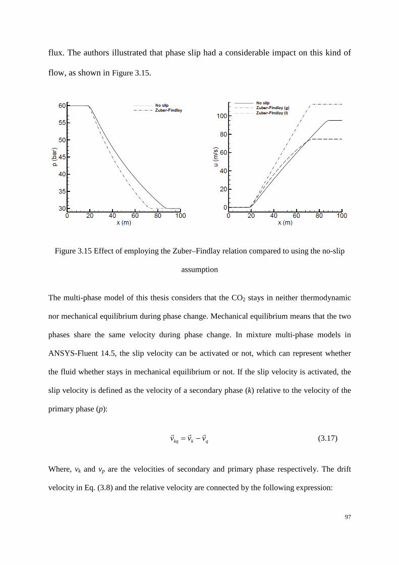
97

flux. The authors illustrated that phase slip had a considerable impact on this kind of

flow, as shown in Figure 3.15.

Figure 3.15 Effect of employing the Zuber–Findlay relation compared to using the no-slip

assumption

The multi-phase model of this thesis considers that the CO2 stays in neither thermodynamic

nor mechanical equilibrium during phase change. Mechanical equilibrium means that the two

phases share the same velocity during phase change. In mixture multi-phase models in

ANSYS-Fluent 14.5, the slip velocity can be activated or not, which can represent whether

the fluid whether stays in mechanical equilibrium or not. If the slip velocity is activated, the

slip velocity is defined as the velocity of a secondary phase (k) relative to the velocity of the

primary phase (p):

qkkq vvv −= (3.17)

Where, vk and vp are the velocities of secondary and primary phase respectively. The drift

velocity in Eq. (3.8) and the relative velocity are connected by the following expression:

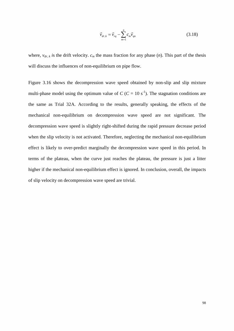
98

∑=

−=n

mqnmrqkdr vcvv

1,

(3.18)

where, vdr, k is the drift velocity. cm the mass fraction for any phase (n). This part of the thesis

will discuss the influences of non-equilibrium on pipe flow.

Figure 3.16 shows the decompression wave speed obtained by non-slip and slip mixture

multi-phase model using the optimum value of C (C = 10 s-1). The stagnation conditions are

the same as Trial 32A. According to the results, generally speaking, the effects of the

mechanical non-equilibrium on decompression wave speed are not significant. The

decompression wave speed is slightly right-shifted during the rapid pressure decrease period

when the slip velocity is not activated. Therefore, neglecting the mechanical non-equilibrium

effect is likely to over-predict marginally the decompression wave speed in this period. In

terms of the plateau, when the curve just reaches the plateau, the pressure is just a litter

higher if the mechanical non-equilibrium effect is ignored. In conclusion, overall, the impacts

of slip velocity on decompression wave speed are trivial.

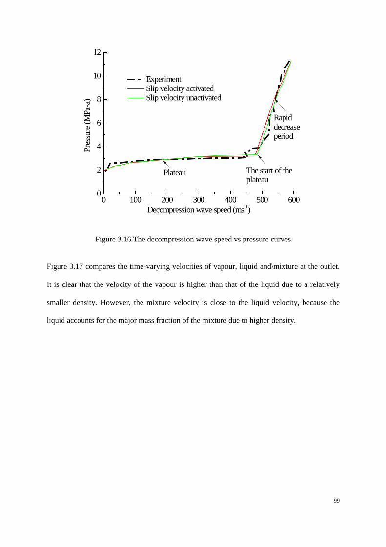
99

0 100 200 300 400 500 6000

2

4

6

8

10

12

Experiment Slip velocity activated Slip velocity unactivated

Pres

sure

(MPa

-a)

Decompression wave speed (ms-1)

Plateau

Rapiddecreaseperiod

The start of the plateau

Figure 3.16 The decompression wave speed vs pressure curves

Figure 3.17 compares the time-varying velocities of vapour, liquid and\mixture at the outlet.

It is clear that the velocity of the vapour is higher than that of the liquid due to a relatively

smaller density. However, the mixture velocity is close to the liquid velocity, because the

liquid accounts for the major mass fraction of the mixture due to higher density.

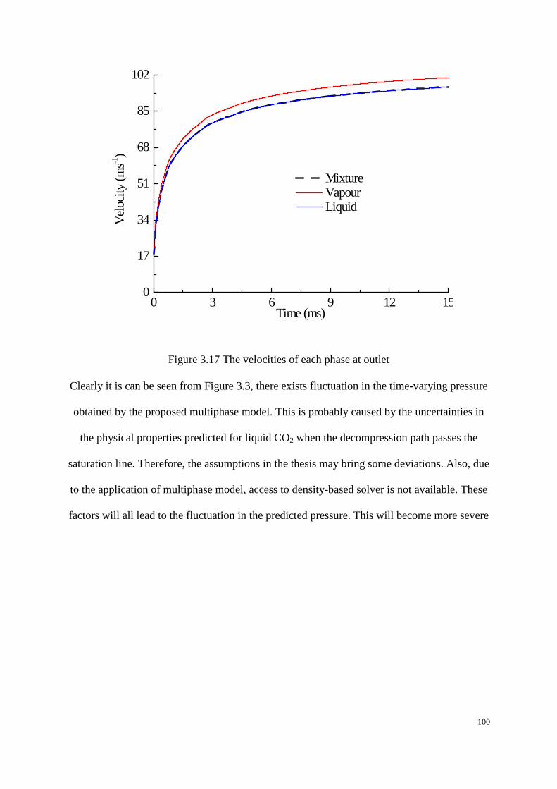
100

0 3 6 9 12 150

17

34

51

68

85

102

Velo

city

(ms-1

)

Time (ms)

Mixture Vapour Liquid

Figure 3.17 The velocities of each phase at outlet

Clearly it is can be seen from Figure 3.3, there exists fluctuation in the time-varying pressure

obtained by the proposed multiphase model. This is probably caused by the uncertainties in

the physical properties predicted for liquid CO2 when the decompression path passes the

saturation line. Therefore, the assumptions in the thesis may bring some deviations. Also, due

to the application of multiphase model, access to density-based solver is not available. These

factors will all lead to the fluctuation in the predicted pressure. This will become more severe

101

at locations near the exit. Therefore, in the present study, PT2 which is 200 mm from the exit

is chosen.

100 200 300 400 500 600

2

4

6

8

10

12

Pres

sure

(MPa

-a)

Decompression wave speed (ms-1)

Experiment GERG-HEM PT2 PT6

Figure 3.18 Comparison of local decompression wave speed at PT2 and PT6 ((C=10 ms-1)

3.4 Summary

In this study, a multi-phase CFD model is presented to simulate the decompression behaviour

of high-pressure CO2 pipelines. GERG-2008 EOS was incorporated into the CFD code to

model the thermodynamic properties of CO2 in both liquid and vapour states. The inter-phase

mass transfer rate was controlled using a mass transfer coefficient in the mass source term.

An energy source term was introduced for energy balance to take into account the latent heat

due to vaporisation. The proposed model was validated against a ‘shock tube’ test conducted

by Botros et al. [46]. As the proposed model enabled the simulation of delayed nucleation

phenomena during the depressurisation process, the effects of the delayed nucleation on the

CO2 decompression characteristics were investigated.

In the present multi-phase decompression model, if the mass transfer coefficient is fine-tuned,

a good agreement with the measurements can be predicted. Not only the decompression wave

speed during the sharp pressure drop period can be predicted quite well, the plateau pressure

and the gradually decrease trend of the plateau can also be successfully simulated. On the

102

contrary, the HEM tends to over-predict the decompression wave speed during the sharp

pressure drop period, and also over-predict the plateau pressure considerably. Furthermore,

HEM cannot predict the gradual decrease trend of the plateau.

Delayed nucleation phenomena have significant influence on the decompression wave speed

during high-pressure CO2 depressurisation. Delayed nucleation results in higher speed of

sound and higher decompression wave speed at a relatively high pressure. Also, the delayed

nucleation leads to the phase change inside the pipeline occurring at a pressure lower than the

saturation pressure. This may be the cause of the discrepancies in the prediction of

decompression wave speed using HEM.

Simulation results of the shock tube test suggests that the optimum mass transfer coefficient

C for a transient CO2 pipeline release from a stagnation pressure of 11 MPa should be around

10 s-1.

The vapour velocity tends to be higher than liquid velocity. The impacts of the mechanical

non-equilibrium effect on decompression wave speed are trivial.

103

Chapter 4 Multi-phase decompression modelling of CO2 mixture

considering non-equilibrium phase transfer

104

Nomenclature

c speed of shound C mass transfer coefficient cp specific heat H enthalpy h latent heat/hill height

ID pipe internal diameter M mass transfer rate P pressure Q mass flow rate q heat flux S source term T temperature t time u velocity W decompression wave speed x location

4.1 Introduction

The anthropogenic CO2 that features in CCS projects usually contains impurities. Although

the amount of these impurities may be small, their existence can change the thermo-physical

properties significantly. In turn, the decompression behaviour will be affected due to a

change of the ‘phase envelope’. Figure 4.1 shows phase envelopes of different CO2 mixtures

and the saturation line of pure CO2. For a given mixture, the phase envelope consists of two

lines – a bubble line (the upper line) and a dew line (the lower line). Above the bubble line,

the fluid is in a liquid state. Between the bubble line and the dew line, the fluid will be in a

two-phase region. This region does not exist for pure CO2. Under the dew line, the fluid is in

a vapour state. Compared against the phase change condition of the mixture, specifically for

the bubble line, the saturation pressure of CO2 is much lower. This leads to a considerable

difference in the decompression behaviour between pure CO2 and CO2 mixtures. The

105

impurity also leads to the curve (curve 1) in Figure 1.4 left shifting markedly due to the

increase of pressure plateau, resulting in a higher toughness requirement.

Figure 4.1 Phase envelop for CO2 mixture and saturation line for pure CO2 (Generated by

GERG-2008)

Several researchers have recently presented their models for CO2 mixture decompression [18,

73]. However, compared with the measured, the deviation is still great. The deviation is also

considered to be brought about by the non-equilibrium assumption. However, there is still not

any study for non-equilibrium effects on CO2 mixture decompression to date. With

incorporating the GERG-2008 EOS into ANSYS Fluent, this chapter focuses on the

impurity/impurities on the non-equilibrium effects for CO2 mixture decompression.

4.2 Methodology

For pure CO2, traditional HEMs have considered that the phase transfer is instantaneous at

saturation pressure; therefore, the pressure is considered at saturation pressure during phase

change. The pressure cannot drop below saturation pressure unless CO2 transfer from the

liquid phase to vapour phase completely. However, actually, in case of the decompression of

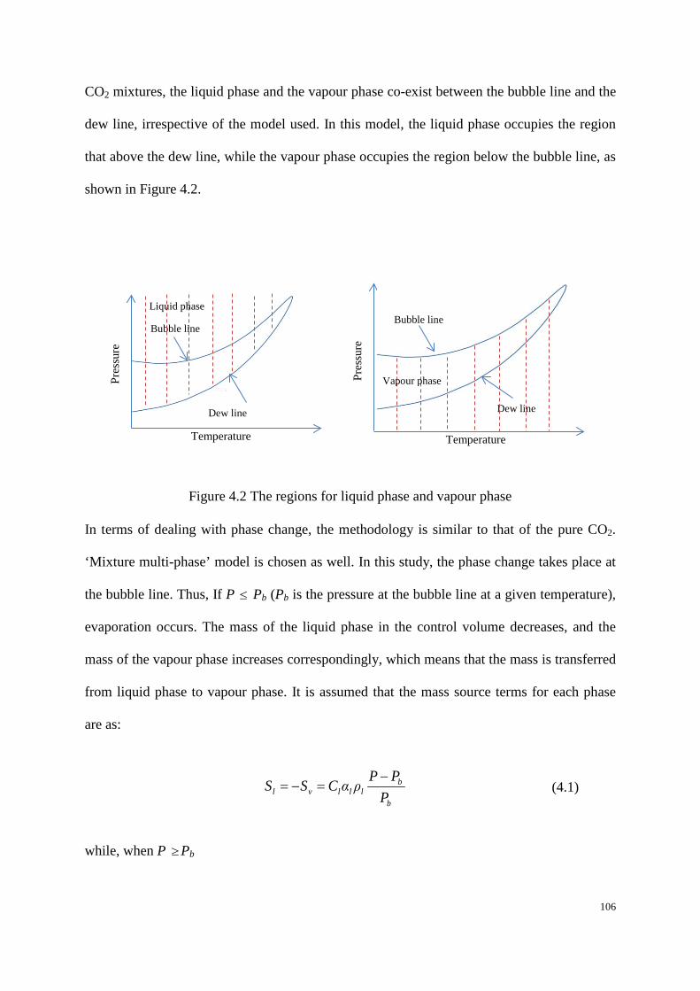
106

CO2 mixtures, the liquid phase and the vapour phase co-exist between the bubble line and the

dew line, irrespective of the model used. In this model, the liquid phase occupies the region

that above the dew line, while the vapour phase occupies the region below the bubble line, as

shown in Figure 4.2.

Figure 4.2 The regions for liquid phase and vapour phase

In terms of dealing with phase change, the methodology is similar to that of the pure CO2.

‘Mixture multi-phase’ model is chosen as well. In this study, the phase change takes place at

the bubble line. Thus, If P ≤ Pb (Pb is the pressure at the bubble line at a given temperature),

evaporation occurs. The mass of the liquid phase in the control volume decreases, and the

mass of the vapour phase increases correspondingly, which means that the mass is transferred

from liquid phase to vapour phase. It is assumed that the mass source terms for each phase

are as:

b

blllvl P

PPραCSS −=−= (4.1)

while, when P ≥ Pb

Temperature

Bubble line

Dew line

Vapour phase Pres

sure

Bubble line

Dew line

Liquid phase

Temperature

Pres

sure

107

b

bvvvvl p

PPραCSS −=−= (4.2)

In this model, it is assumed that C=Cl=CV. Two shock tube tests (Trial 20A and Trial 24A)

conducted by Botros et al. [150] were used to validate the two-phase model proposed in this

thesis. In Trial 20A, a CO2-N2 mixture was tested. The stagnation conditions were: P0 =

14.011 MPa and T0 = 278.72 K. The mole fractions of each component in the mixture were

CO2 94.58% and N2 5.42%. Trial 24A used a CO2-O2 mixture, with stagnation conditions of

P0 = 14.654 MPa and T0 = 278.21 k, respectively, and the mole fractions of each component

in the mixture were CO2: 96.4% and O2 3.6%.

The CFD models were set up to simulate Trials 20A and 24A. Also, in order to compare the

decompression behaviour with that of pure CO2, Trial 32A (Pure CO2, P0 = 11.27 MPa, T0 =

281.89 K) was also simulated. In the transient CFD model, the pressure and temperature were

monitored at several locations near the outlet plane, where pressure transducers and

temperature probes were installed in the physical experiment. The locations of the pressure

transducers and temperature probes have been given in Table 3-1.

4.3 Results and discussion

Due to the delayed nucleation, as for pure CO2, decompression will pass the saturation line.

When it passes the saturation line, the properties of liquid CO2 are assumed to be equal to

those on the saturation line, because there is no better alternative. However, GERG provides

the liquid and vapour’s properties in the two-phase region, respectively. Therefore, relatively

real properties can be used in this region.

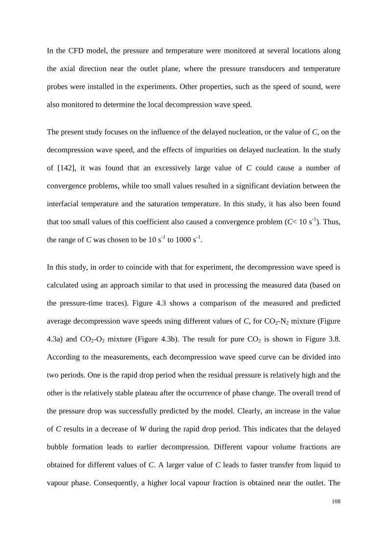
108

In the CFD model, the pressure and temperature were monitored at several locations along

the axial direction near the outlet plane, where the pressure transducers and temperature

probes were installed in the experiments. Other properties, such as the speed of sound, were

also monitored to determine the local decompression wave speed.

The present study focuses on the influence of the delayed nucleation, or the value of C, on the

decompression wave speed, and the effects of impurities on delayed nucleation. In the study

of [142], it was found that an excessively large value of C could cause a number of

convergence problems, while too small values resulted in a significant deviation between the

interfacial temperature and the saturation temperature. In this study, it has also been found

that too small values of this coefficient also caused a convergence problem (C< 10 s-1). Thus,

the range of C was chosen to be 10 s-1 to 1000 s-1.

In this study, in order to coincide with that for experiment, the decompression wave speed is

calculated using an approach similar to that used in processing the measured data (based on

the pressure-time traces). Figure 4.3 shows a comparison of the measured and predicted

average decompression wave speeds using different values of C, for CO2-N2 mixture (Figure

4.3a) and CO2-O2 mixture (Figure 4.3b). The result for pure CO2 is shown in Figure 3.8.

According to the measurements, each decompression wave speed curve can be divided into

two periods. One is the rapid drop period when the residual pressure is relatively high and the

other is the relatively stable plateau after the occurrence of phase change. The overall trend of

the pressure drop was successfully predicted by the model. Clearly, an increase in the value

of C results in a decrease of W during the rapid drop period. This indicates that the delayed

bubble formation leads to earlier decompression. Different vapour volume fractions are

obtained for different values of C. A larger value of C leads to faster transfer from liquid to

vapour phase. Consequently, a higher local vapour fraction is obtained near the outlet. The

109

vapour phase tends to occupy more space due to its much smaller density compared to the

liquid phase. Therefore, a larger fraction of vapour impedes the reduction of pressure due to

the average methodology to obtain the decompression wave speed. In general, W obtained by

the model with C = 100 s-1, 50 s-1 and 10 s-1 best agrees with measurements for CO2-N2

mixture, CO2-O2 mixture and pure CO2 respectively, during this period.

More importantly, the abrupt drop in the decompression wave speed curve which created the

long pressure plateau is predicted successfully by this model. HEM tends to over-predict the

plateau pressures, for both pure CO2 and CO2 mixtures. Clearly, the plateau pressure of CO2

mixtures is much higher than that of pure CO2. This is because the pressure at the bubble line

for the mixture is much higher than the saturation pressure of pure CO2, at the corresponding

temperature. Therefore, the phase change will start at a relatively higher pressure. The phase

change continues to take place in the ‘wide’ region between the bubble line and the dew line

for a CO2 mixture, until the pressure falls below the dew line. However, for pure CO2, the

phase change occurs when the pressure crosses the saturation line. Thus, the situation is quite

different for CO2 mixtures compared to pure CO2. But, obviously, when the smaller the value

of C, the lower the plateau pressures, for both pure CO2 and for CO2 mixtures. According to

Figure 4.3 and Figure 3.8, the results obtained by using C = 50 s-1, C = 15 s-1 and C = 10 s-1,

have the best agreement with experimental data in the plateau, for the CO2-N2 mixture, the

CO2-O2 mixture and pure CO2, respectively. Obviously, according to the predicted results of

the plateau pressure, the optimal values of C for pure CO2 and CO2 with different impurities

are quite different. Therefore, it can be concluded that impurities in CO2 affect the delayed

bubble formation significantly. One possible reason is that the impurities change the fluid’s

thermodynamic properties greatly. Also, the formation mechanism of the “bubble line” in

mixture differs from that of the “saturation line” in pure CO2. The pressures at bubble lines

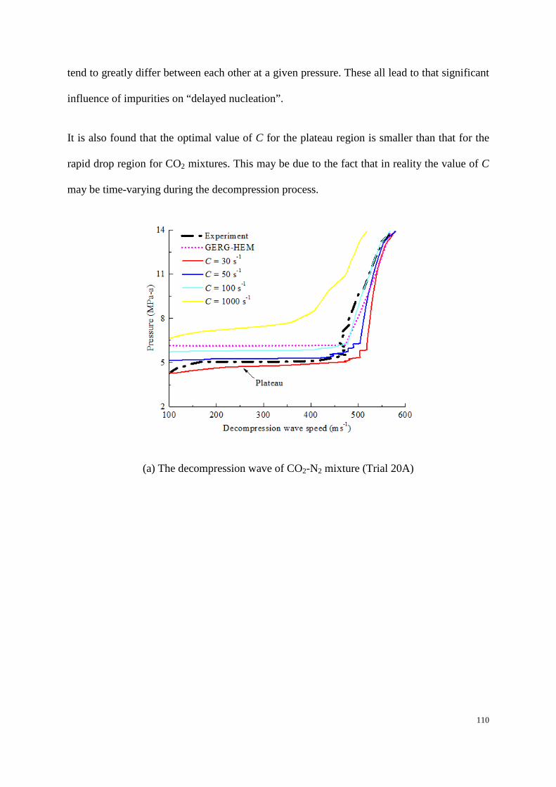
110

tend to greatly differ between each other at a given pressure. These all lead to that significant

influence of impurities on “delayed nucleation”.

It is also found that the optimal value of C for the plateau region is smaller than that for the

rapid drop region for CO2 mixtures. This may be due to the fact that in reality the value of C

may be time-varying during the decompression process.

(a) The decompression wave of CO2-N2 mixture (Trial 20A)

111

(b) The decompression wave of CO2-O2 mixture (Trial 24A)

Figure 4.3 Comparison of the measured and simulated decompression wave speeds

Figure 4.4a and 4.4b display the P-T curves obtained for the CO2-N2 mixture (Figure 4.4a),

and the CO2-O2 mixture (Figure 4.4b), respectively. Both the P-T curves obtained from the

location in PT2. The result for pure CO2 is shown in Figure 3.4. Clearly, the thermodynamic

trajectories obtained for various values of C as well as the isentrope obtained using GERG-

HEM are very close before reaching the saturation line or the bubble line. During this period,

phase change does not occur in the control volume. Consequently the value of C has nearly

no influence on the thermodynamic trajectory. However, after touching the saturation

pressure or the bubble line, discrepancies are seen. For pure CO2, the pressure drops rapidly

with very small temperature drop after crossing the saturation line. After the initial drop, the

pressure returns to a much higher value and starts to decrease again afterwards for a while.

Eventually the P-T curve tends to approach the saturation line. In contrast, the P-T curve

predicted by GERG-HEM will follow the saturation curve after touching it. This is the reason

112

for the over-prediction of the plateau pressure when using HEM. For CO2 mixtures, the P-T

curves obtained by both HEM and the multi-phase model can cross the bubble line, arriving

at the ‘two-phase’ region. Compared to that obtained by the multi-phase model, after crossing

the bubble line, the P-T curve obtained by HEM will deviate much less from the bubble line.

The P-T curves predicted by the multi-phase model deviate significantly from the bubble line

and will end up nearly parallel to the bubble line. A small value of C creates a larger

deviation from the bubble line. As a result, the pressure in the two-phase region will be lower.

When the value of C is small enough, the P-T curve will not only pass the bubble line, but

also cross the dew line, reaching a much lower pressure. It can be inferred that the delayed

bubble formation influences the decompression wave speed, and the over-prediction of

plateau pressure by HEM is most likely to be because this phenomenon is not accounted for.

(a) The P-T curves for CO2-N2 mixture (Trial 20A)

113

(b) The P-T curves for CO2-O2 mixture (Trial 24A)

Figure 4.4 The P-T curves (thermodynamic trajectories) during the decompression

Figure 4.5 shows the pressure as a function of vapour volume fraction as predicted by the

multi-phase model for different values of C as well as that obtained by HEM, for the CO2-N2

mixture (Figure 4.5a) and the CO2-O2 mixture (Figure 4.5b),which are obtained at PT2.

Clearly, a smaller value of C results in a lower vapour volume fraction at a given pressure

due to lower mass transfer rate. It is also observed that compared with the vapour volume

fraction predicted by HEM, there is more deviation when a smaller value of C is chosen. The

curves predicted by the multi-phase model are close to that predicted by HEM when C =

1000 s-1, for both the CO2-N2 mixture and the CO2-O2 mixture. One can assume that when

using a sufficiently large value of C, the fluid will reach an equilibrium state. The density and

speed of sound in the vapour are much smaller than those in the liquid, thus a larger value of

C will underestimate the density and the speed of sound in the ‘two-phase’ region, because a

larger value of C leads to a larger vapour fraction in the cells. This may also explain why the

decompression wave speed is significantly smaller when a larger value of C is chosen. Also,

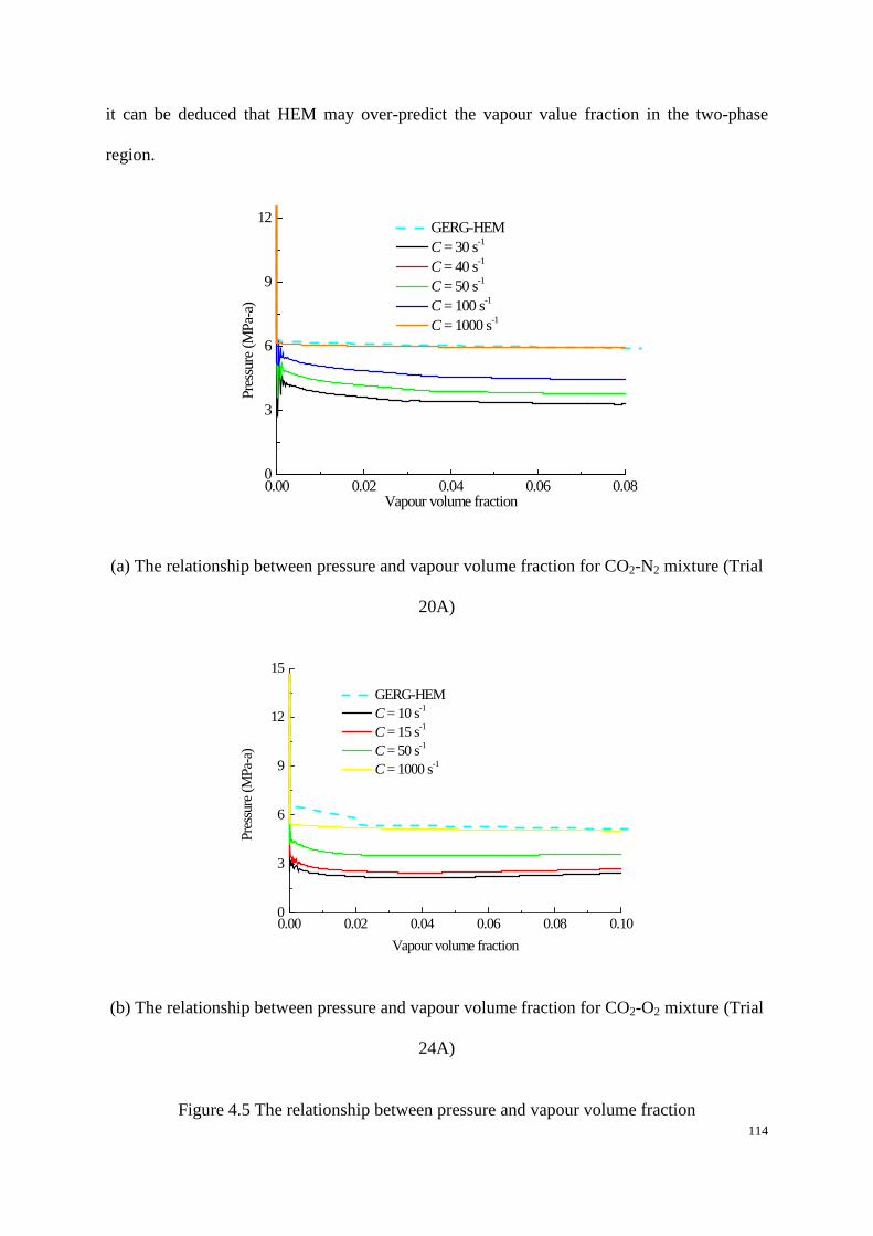
114

it can be deduced that HEM may over-predict the vapour value fraction in the two-phase

region.

0.00 0.02 0.04 0.06 0.080

3

6

9

12

Pres

sure

(MPa

-a)

Vapour volume fraction

GERG-HEM C = 30 s-1

C = 40 s-1

C = 50 s-1

C = 100 s-1

C = 1000 s-1

(a) The relationship between pressure and vapour volume fraction for CO2-N2 mixture (Trial

20A)

0.00 0.02 0.04 0.06 0.08 0.100

3

6

9

12

15

Pres

sure

(MPa

-a)

Vapour volume fraction

GERG-HEM C = 10 s-1

C = 15 s-1

C = 50 s-1

C = 1000 s-1

(b) The relationship between pressure and vapour volume fraction for CO2-O2 mixture (Trial

24A)

Figure 4.5 The relationship between pressure and vapour volume fraction

115

The great deviation between decompression wave speeds obtained by HEM and those

predicted by the multi-phase model with a larger value of C is probably due to the calculation

method of the decompression wave speed. As for GERG-HEM proposed by Botros et al

[150], decompression wave speed is calculated by Eq. (2.20) (the speed of sound minus the

local out flow velocity) rather than performing a linear regression of each isobar curve which

is used in the experiment and the multi-phase model. The speed of sound is defined from the

given pressure and temperature, which is obtained from the isentropic path at the

corresponding pressure. However, the usefulness of this depends on the real accuracy of the

pressure. Figure 4.6 shows the decompression wave speed obtained by the speed of sound

minus the escaping out flow velocity at point PT2 (CO2-N2 test, Trial 20A). Apparently, the

decompression wave speed obtained by C = 1000 s-1 is close to that obtained by GERG-HEM.

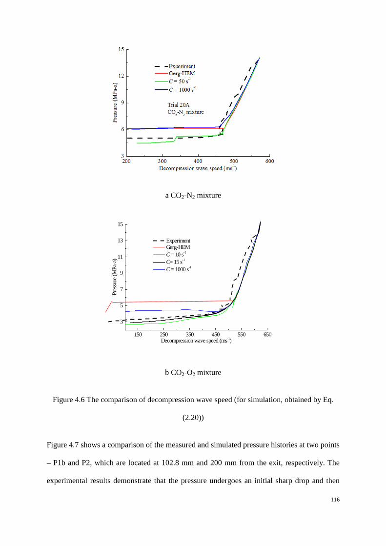
116

a CO2-N2 mixture

150 250 350 450 550 650

3

5

7

9

11

13

15

Pres

sure

(MPa

-a)

Decompression wave speed (ms-1)

Experiment Gerg-HEM C = 10 s-1

C= 15 s-1

C = 1000 s-1

b CO2-O2 mixture

Figure 4.6 The comparison of decompression wave speed (for simulation, obtained by Eq.

(2.20))

Figure 4.7 shows a comparison of the measured and simulated pressure histories at two points

– P1b and P2, which are located at 102.8 mm and 200 mm from the exit, respectively. The

experimental results demonstrate that the pressure undergoes an initial sharp drop and then

117

remains at a relatively stable plateau. The overall trend of the pressure drop was successfully

predicted by the multi-phase model. However, it is clear that the approach of the pressure

transients to the plateau is significantly affected by the non-equilibrium phase transition (i.e.

the value of C used). In addition, the predicted pressure curve is lower at the plateau when a

smaller value of C is chosen. The pressure transient predicted using C = 50 s-1 shows best

agreement with measurements near the plateau.

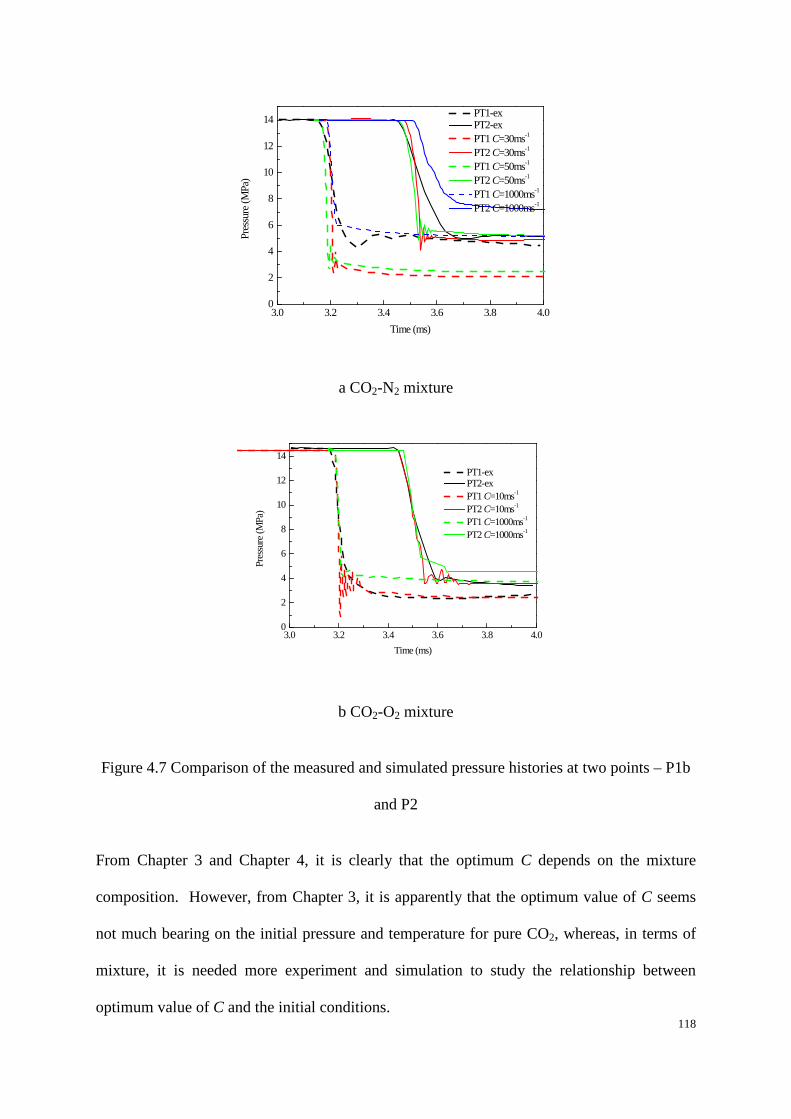
118

3.0 3.2 3.4 3.6 3.8 4.00

2

4

6

8

10

12

14

Pres

sure

(MPa

)

Time (ms)

PT1-ex PT2-ex PT1 C=30ms-1

PT2 C=30ms-1

PT1 C=50ms-1

PT2 C=50ms-1

PT1 C=1000ms-1

PT2 C=1000ms-1

a CO2-N2 mixture

3.0 3.2 3.4 3.6 3.8 4.00

2

4

6

8

10

12

14

Pres

sure

(MPa

)

Time (ms)

PT1-ex PT2-ex PT1 C=10ms-1

PT2 C=10ms-1

PT1 C=1000ms-1

PT2 C=1000ms-1

b CO2-O2 mixture

Figure 4.7 Comparison of the measured and simulated pressure histories at two points – P1b

and P2

From Chapter 3 and Chapter 4, it is clearly that the optimum C depends on the mixture

composition. However, from Chapter 3, it is apparently that the optimum value of C seems

not much bearing on the initial pressure and temperature for pure CO2, whereas, in terms of

mixture, it is needed more experiment and simulation to study the relationship between

optimum value of C and the initial conditions.

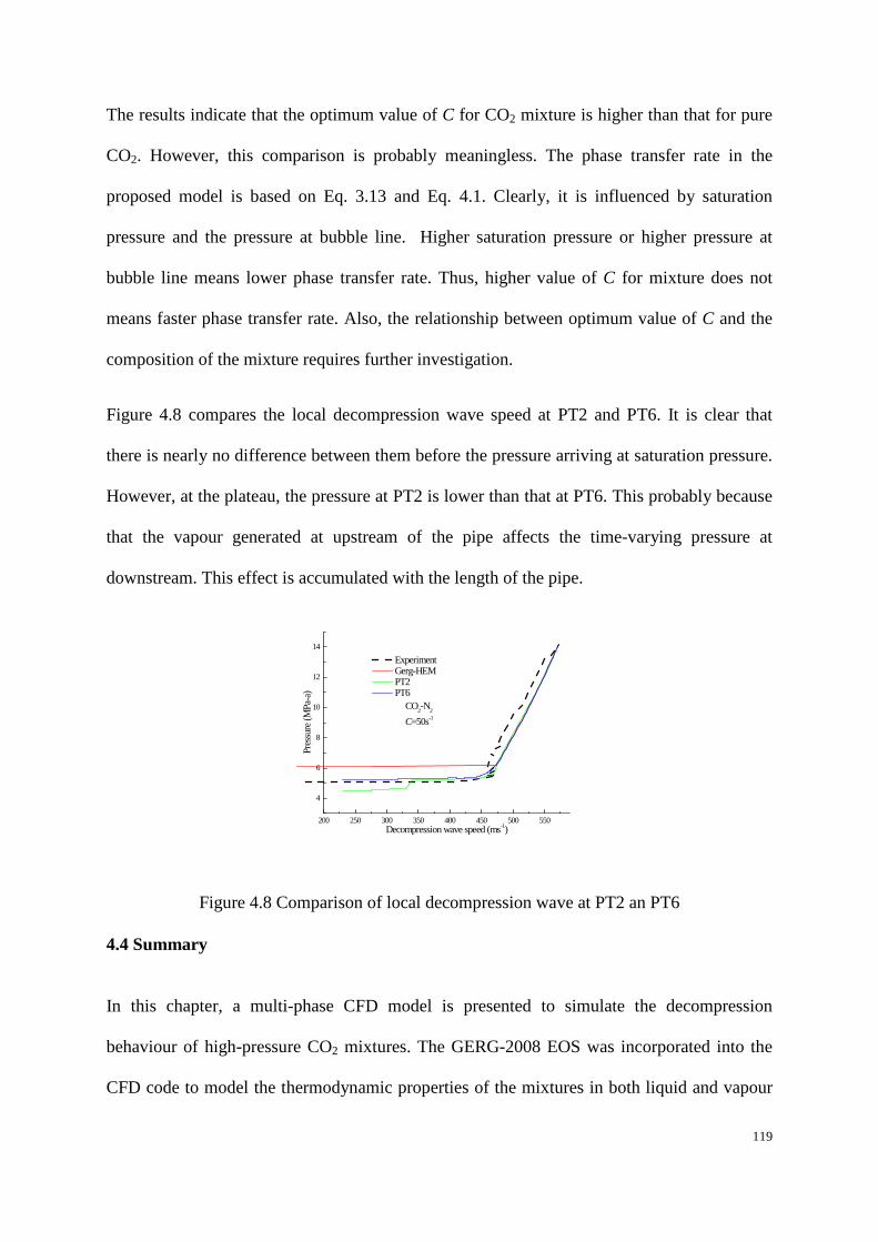
119

The results indicate that the optimum value of C for CO2 mixture is higher than that for pure

CO2. However, this comparison is probably meaningless. The phase transfer rate in the

proposed model is based on Eq. 3.13 and Eq. 4.1. Clearly, it is influenced by saturation

pressure and the pressure at bubble line. Higher saturation pressure or higher pressure at

bubble line means lower phase transfer rate. Thus, higher value of C for mixture does not

means faster phase transfer rate. Also, the relationship between optimum value of C and the

composition of the mixture requires further investigation.

Figure 4.8 compares the local decompression wave speed at PT2 and PT6. It is clear that

there is nearly no difference between them before the pressure arriving at saturation pressure.

However, at the plateau, the pressure at PT2 is lower than that at PT6. This probably because

that the vapour generated at upstream of the pipe affects the time-varying pressure at

downstream. This effect is accumulated with the length of the pipe.

200 250 300 350 400 450 500 550

4

6

8

10

12

14

Pres

sure

(MPa

-a)

Decompression wave speed (ms-1)

Experiment Gerg-HEM PT2 PT6

CO2-N2

C=50s-1

Figure 4.8 Comparison of local decompression wave at PT2 an PT6

4.4 Summary

In this chapter, a multi-phase CFD model is presented to simulate the decompression

behaviour of high-pressure CO2 mixtures. The GERG-2008 EOS was incorporated into the

CFD code to model the thermodynamic properties of the mixtures in both liquid and vapour

120

states. The inter-phase mass transfer rate was controlled using a time relaxation factor in the

mass source term. An energy source term was introduced for energy balance to take into

account the latent heat due to vaporisation. The proposed model was validated against ‘shock

tube’ tests conducted by Botros et al. As the proposed model enabled the simulation of

delayed bubble formation phenomena during the depressurisation process, the effects of

delayed bubble formation on the CO2 mixture decompression characteristics were

investigated, and the influence of impurities on delayed bubble formation also studied.

It was found that the delayed bubble formation has a considerable effect on the

decompression behaviour. The delayed bubble formation leads to the fact that the phase

change inside the pipeline occurs at a pressure much lower than the pressure at the bubble

line. This may be the reason for discrepancies in the prediction of decompression wave speed

using HEM. Also, the delayed bubble formation results in a higher liquid volume fraction in

the two-phase region, which means a higher speed of sound and higher decompression wave

speed. Simulations of the shock tube tests show that if the mass transfer coefficient in the

multi-phase model is fine-tuned, the plateau pressure which is crucial to pipeline fracture

control can be predicted reasonably well.

The simulation results also suggest that the optimum value of the mass transfer coefficient C

may be time-varying during the depressurisation procedure. If only the prediction of the

plateau pressure is considered, the optimum time relaxation factor C for the mixture which

contains 94.58% CO2 and 5.42% N2 released from a stagnation pressure of 14 MPa should be

around 50 s-1. The optimal C for the mixture which contains 96.4% CO2 and 3.6% O2

released from a stagnation pressure of 14.7 MPa should be around 15 s-1. Comparison with

the results of the decompression of pure CO2 shows that the impurities in CO2 affect the

delayed bubble formation significantly.

121

Chapter 5 CFD simulation of under-expanded CO2 jet

122

Nomenclature

A cross-sectional area c speed of shound Dt turbulent diffusivity k kinetic energy M mass transfer rate P pressure

Sct turbulent Schmidt number T temperature t time V specific molar volume v velocity

5.1 Introduction

The rupture of a high-pressure CO2 pipeline will be immediately followed by the initiation of

a decompression wave inside the pipeline and an expansion exiting from the orifice (pipe exit)

into the ambient with very high momentum. This complicated process greatly influences the

source strength, such as discharge rate. The source strength surely affects the subsequent

dispersion of the CO2 in the atmosphere. Therefore, to accurately predict the source strength

of a high-pressure CO2 pipeline leakage, a comprehensive study of the characteristics of

under-expanded CO2 jet flows is required. However, detailed investigations of the

characteristics of the under-expanded jet flow have usually been ignored in previous studies,

due to their complexity.

The ideal gas model cannot accurately reflect the properties of CO2 at very high pressure or

very low temperature, and these situations are very common during a CO2 pipeline release.

When using ANSYS Fluent, a user-defined real gas model can be introduced to precisely

model the properties of the gas. In this part, a real gas EOS was used to simulate under-

123

expansion of CO2, which could achieve more accurate source strength prediction and

consequently help the dispersion evaluation.

5.2 Simulation model

In free air jet experiment, the air jet was produced by a nozzle having an exit diameter of 2.7

mm (dz), and operating at a pressure of 6.6 atm. The velocity field measurements were made

using the Fabry–Perot Laser-Doppler technique.

As the expansion time studied is relatively short, the influence of gravity and heat transfer

between the air and CO2 could be ignored. Accordingly, it is feasible to construct a two-

dimensional computational domain to reduce the computational runtime due to the axial

symmetry domain. The axisymmetric computational domain for the simulation of expansion

and the mesh around the nozzle are shown in Figure 5.1. The overall mesh contains 70,000

cells.

Figure 5.1 Computational domain and mesh

5.3 Air jet using user-defined real gas model

An air jet experiment conducted by Eggins et al. [152] is chosen for validating the user-

defined real gas model. In the experiment, high pressure air was released from a converging

nozzle with an exit diameter of 2.7 mm. The stagnation pressure was 6 atm (absolute pressure)

and the stagnation temperature was 293 k. The standard k-ε model was chosen to solve the

turbulent model due to its simplicity. The physical properties of air were calculated at given

300 mm

100

mm

124

pressure and temperature at runtime using P-R real EOS and stored in tables. Figure 5.2

shows the predicted velocity along the axis of the jet, compared with the experimental data,

which was plotted with 5% error bar. It can be found that the velocity is around 380 ms-1 at

pipe exit. The velocity is increasing gradually with the distance until reaching the peak (about

600 m s-1) at around 3.8 mm. After that, the velocity drops significantly and then drops

marginally with the distance. Clearly, the predicted velocities are in good agreement with the

observation. Specially, the trend as well as the peak is predicted well. The predicted

velocities have less than 5% errors for most locations.

Figure 5.2 Comparison of velocity

Figure 5.3 and Figure 5.4 show the predicted transverse velocity profiles at 0.2 mm upstream

and downstream from the Mach disc against the measurements, respectively. The

experimental data plotted with 5% error bars. It can be observed that the highest transverse

velocity occurs at the middle location in terms of profile at 0.2 mm upstream. The transverse

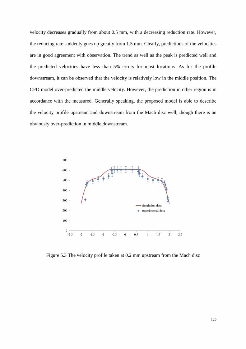
125

velocity decreases gradually from about 0.5 mm, with a decreasing reduction rate. However,

the reducing rate suddenly goes up greatly from 1.5 mm. Clearly, predictions of the velocities

are in good agreement with observation. The trend as well as the peak is predicted well and

the predicted velocities have less than 5% errors for most locations. As for the profile

downstream, it can be observed that the velocity is relatively low in the middle position. The

CFD model over-predicted the middle velocity. However, the prediction in other region is in

accordance with the measured. Generally speaking, the proposed model is able to describe

the velocity profile upstream and downstream from the Mach disc well, though there is an

obviously over-prediction in middle downstream.

Figure 5.3 The velocity profile taken at 0.2 mm upstream from the Mach disc

126

Figure 5.4 The velocity profile taken at 0.2 mm downstream from the Mach disc

Figure 5.5 to Figure 5.7 give the distribution of simulated pressure, temperature and velocity

and much number respectively. Expansion of the jet outside the nozzle is very clear seen. The

lowest temperature is approximately 100 K, just upstream from the Mach disc, where the

velocity is highest. The Mach number shows a similar profile with the velocity. The core and

annulus structure is also clear in the plot of Mach number. The flow structure consists of a

curved region, where the expanding flow is curved back towards the axis because of the

external pressure and a reflect shock. A fully developed Mach disc can be seen. Figure 5.8

shows the profiles of temperature and velocity along the axis. It can be seen that high velocity

generates low temperature due to the conservation of energy. The velocity jumps to the

highest shortly just a little downstream from the nozzle, whereas the temperature drops

drastically in this region. From downstream of the Mach disc, the velocity is reducing and

temperature is rising correspondently. And then the velocity rises again accompanied by a

reduction in temperature. Then the velocity declines gradually to near zero and temperature

goes up to atmosphere temperature.

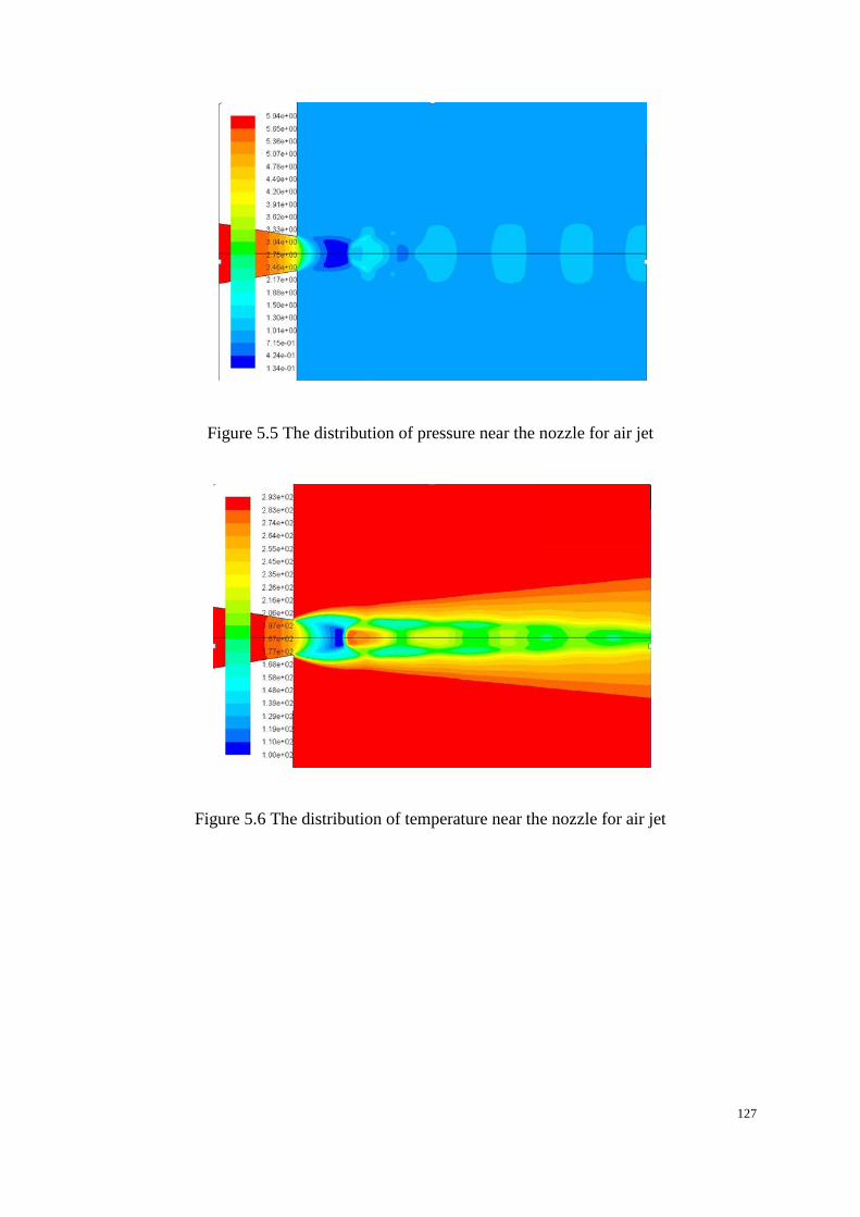
127

Figure 5.5 The distribution of pressure near the nozzle for air jet

Figure 5.6 The distribution of temperature near the nozzle for air jet

128

a velocity

b Mach number

Figure 5.7 The distribution of velocity and Mach number near the nozzle for air jet

129

Figure 5.8 Profiles of temperature and velocity along the axis

5.4 CO2 jet using PR EOS

As described in Section 2.2.2, PR EOS is widely used in the industry. The advantage of this

equation is that it can accurately and easily represent the interrelationship between

temperature, pressure, and phase compositions in binary and multi-component systems.

Implementation of the PR EOS only requires the critical properties and acentric factor as

inputs. Supercritical CO2 can be dealt with in the gaseous phase due to the continuous

property between supercritical state and gaseous state. From the literature review, it has been

found that PR EOS is suitable for modelling the property of CO2 above the triple point. The

subsequent part will simulate the CO2 jet using PR EOS, as it has simple form and proven

accuracy in the modelling of CO2 properties in this condition.

The computational domain and initial conditions are the same as the air jet described in

Section 5.2. The standard k-ε model is chosen. The release process is like leak 5 which was

mentioned in Figure 2.4, from supercritical state to gaseous state.

130

The simulated temperature distribution is shown in Figure 5.9 (planform). Clearly, the

temperature drops considerably near the Mach disk. The lowest temperature is nearly 113 k

due to the Joule-Thompson effect. Downstream from the Mach disc, the temperature becomes

slightly higher. It is also noted that the lowest temperature exists in ‘central line’ before and

near Mach disc. In contrast, the temperature is higher in the ‘central line’ downward from the

Mach disc.

Figure 5.9 The distribution of temperature near the nozzle for CO2 jet

Figure 5.10 shows the distribution of velocity in the nozzle and downstream. The structure of

velocity distribution is similar to that of temperature. The discontinued profile onward and

downward from the Mach disc can be clearly seen. However, the low temperature area tends

to correspond to the high velocity area. The maximum velocity also occurs near the Mach

disc, which is around 498 m/s, and the choke velocity at the exit of the nozzle is about 220

m/s which is close to the speed of sound (Figure 5.11). Clearly, though there exists some

discrepancy between the speed of sound and velocity at nozzle exit, the predicted velocity are

generally consistently close to speed of sound. Figure 5.12 shows the velocity and Mach

number profiles at min velocity disc. It can be seen that there exist a peak in the radial

131

direction for both velocity and Mach number. Obviously, the Mach number is relatively low

near the axis, however, it become higher at around 1.2 mm from the axis. The maximum

Mach number can exceed 2.

a velocity

b Mach number

Figure 5.10 The distribution of velocity and Mach number the nozzle for CO2 jet

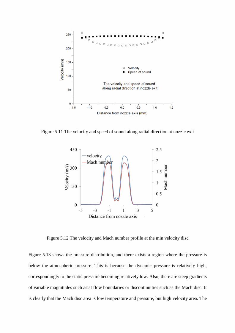
132

Figure 5.11 The velocity and speed of sound along radial direction at nozzle exit

Figure 5.12 The velocity and Mach number profile at the min velocity disc

Figure 5.13 shows the pressure distribution, and there exists a region where the pressure is

below the atmospheric pressure. This is because the dynamic pressure is relatively high,

correspondingly to the static pressure becoming relatively low. Also, there are steep gradients

of variable magnitudes such as at flow boundaries or discontinuities such as the Mach disc. It

is clearly that the Mach disc area is low temperature and pressure, but high velocity area. The

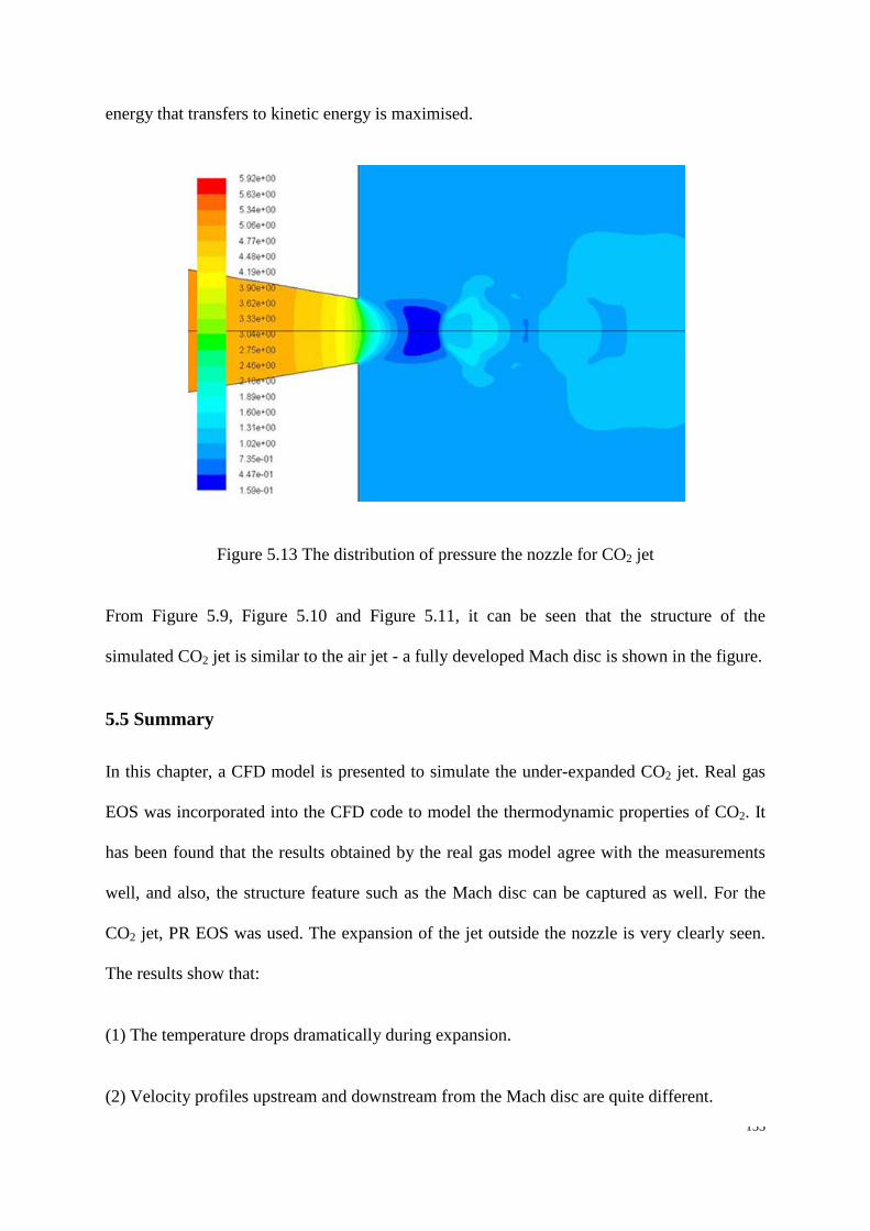
133

energy that transfers to kinetic energy is maximised.

Figure 5.13 The distribution of pressure the nozzle for CO2 jet

From Figure 5.9, Figure 5.10 and Figure 5.11, it can be seen that the structure of the

simulated CO2 jet is similar to the air jet - a fully developed Mach disc is shown in the figure.

5.5 Summary

In this chapter, a CFD model is presented to simulate the under-expanded CO2 jet. Real gas

EOS was incorporated into the CFD code to model the thermodynamic properties of CO2. It

has been found that the results obtained by the real gas model agree with the measurements

well, and also, the structure feature such as the Mach disc can be captured as well. For the

CO2 jet, PR EOS was used. The expansion of the jet outside the nozzle is very clearly seen.

The results show that:

(1) The temperature drops dramatically during expansion.

(2) Velocity profiles upstream and downstream from the Mach disc are quite different.

134

(3) The upstream Mach disc area is a low temperature and pressure, but high velocity area.

135

Chapter 6 CFD simulation of CO2 dispersion in a complex environment

136

Nomenclature

H buliding height h hill height k kinetic energy L base radius of the hill t time u velocity

ur reference wind velocity V specific molar volume v velocity x distance

In order to quantitatively evaluate the risk associated with the CCS technology, a deeper

understanding of CO2 dispersion resulting from accidental releases is essential. CO2 is a

heavier-than-air gas. Its dispersion patterns may vary according to local conditions. This

study focuses on CO2 dispersion over complex terrains. CFD models were developed to

simulate the CO2 dispersion over four hypothetical topographies: (1) a flat terrain with an

axisymmetric hill and (2) a flat terrain with two axisymmetric hills (3) a simplified model of

an urban area with buildings and (4) a real terrain in Australia. The source strength, wind

velocity and height of the buildings were varied to investigate their effects on the dispersion

profile. This chapter may offer a viable method for assessment of risks associated with CCS.

6.1 Introduction

CO2 released from pipelines can disperse downwind, potentially affecting populations and the

environment. Therefore, obtaining a deeper understanding of the dispersion of CO2 released

from pipelines under different conditions is essential for assessing the safety of the technique.

In recent years, a number of models have been proposed to estimate the atmospheric

dispersion of gases resulting from accidental or planned release. These can be classified into

137

three categories: (a) “Gaussian-based” models, (b) “Similarity-profile” models, and (c)

Computational fluid dynamics (CFD) models [107]. CFD models use more detailed

mathematical descriptions of the conservation principles, allowing the simulation of complex

physical processes involving heat and mass transport in complicated computational domains.

Although time-consuming, CFD models are more appropriate for the modelling of dispersion

over complex terrains and under different meteorological conditions. Using CFD for

dispersion modelling in all its complexity (terrain topography, presence of obstacles, etc.) is a

relatively recent development [3, 21, 114, 116, 118, 119, 126, 153]. In the past decades, a few

researchers have used general-purpose CFD packages (such as Fluent or CFX) for

atmospheric dispersion modelling [21, 126, 153, 154], while others have relied on CFD

software packages (such as fluidyn-PANACHE) designed specifically for atmospheric

dispersion modelling [114, 155].

Although numerical simulation of the atmospheric dispersion of hazardous gases over flat

terrains using CFD is a relatively recent development, there have been some reports in the

literature. Labovsky and Jelemensky [154] used the CFD software Fluent to model the

dispersion of ammonia in the ‘Fladis’ field experiments. They found that it was important to

model the turbulence level appropriately. Mazzoldi et al. [114] evaluated the suitability of the

dispersion simulation tool fluidyn-PANACHE using data from the Prairie Grass and Kit Fox

field experiments for validation. Xing et al. [153] carried out a scaled experiment on a CO2

release for the purpose of measuring the downwind concentration levels. In their experiment,

the CO2 was released vertically from a circular source at ground level at different flow rates.

In addition, CFD simulations were carried out using different turbulence models. They

concluded that the results of simulations using the k−ε and shear stress transport (SST) k−ω

turbulence models were in acceptable agreement with the experimental data. Mazzoldi et al.

[21] compared two atmospheric dispersion models, the Gaussian model and a CFD model,

138

taking representative input parameters for high-pressure CO2 releases. Results showed a

lowering of the risk involved in the transportation of CO2 by up to one order of magnitude,

when modelling the same releases with a CFD tool, compared to the more widespread

Gaussian models. Liu et al. [3] used CFD techniques to simulate the atmospheric dispersion

of CO2 released from a high-pressure pipeline. Two cases in the CO2 dispersion experiments

carried out by DNV BP (Trial DF1) [156] were simulated for validation, and DNV Phast was

employed for comparative studies. The above studies suggested that realistic representations

of the ‘Atmospheric Boundary Layer’ and turbulence levels are crucial in CFD modelling.

Mocellin et al. [128] simulated the accident release of CO2 from CCS pipelines and the

consequences related to sublimating dry ice bank that may occur. Results showed that serious

risks were associated with the sublimating the dry ice bank near the release point and the

hazards increase with a decreasing mean wind speed and a rise in ambient temperature.

In recent years, modelling of hazardous gas dispersion over complex terrains has attracted

increasing attention. McBride et al. [157] simulated the dispersion of chlorine and found that

complex terrain and buildings affected not only the downwind hazard range, but also the

width of the dispersion cloud and its direction of travel. Chow et al. [158] proposed a model

to simulate the atmospheric dispersion of CO2 resulting from a leakage. The results

demonstrated that even small topographical features had a notable effect on the dispersion of

the heavy gas. Scargiali et al. [127] simulated the formation of toxic clouds of a heavy gas in

an urban area using the CFD package ANSYS CFX. The simulation strategy involved a

steady-state simulation to establish the pre-release wind velocity field, followed by a transient

after-release simulation. The computational domain was modelled as a simple network of

straight roads with regularly distributed blocks mimicking buildings. Results showed that the

presence of buildings lowered the maximum concentration and enhanced the lateral spread of

the cloud. Dispersion dynamics were also found to be strongly affected by the quantity of the

139

heavy gas released. Tauseef et al. [118] applied CFD techniques in an assessment of heavy

gas dispersion in the presence of a cubical obstacle downstream of the source. The

performance of different turbulence models was investigated. They found that the realizable

k-ε model is slightly superior. Hsieh et al. [126] studied the dispersion of CO2 from a CCS-

related infrastructure in a complex hypothetical topography. The simulated predicted

concentration levels were found to be reasonable. Overall, the presence of an obstacle and/or

complex terrain has a significant influence on heavy gas dispersion. Generally speaking, the

research associated with CO2 dispersion over complex terrains is in its early stages. For

quantification of the risks associated with CO2 dispersion, an appropriate dispersion model

especially over complex terrains is essential.

The present study focuses on CO2 dispersion over complex terrains using CFD techniques.

Three hypothetical topographies, a flat terrain with an axisymmetric hill and two hills a

model urban area with buildings, and a real terrain in Australia were chosen to investigate the

topographical effects on the dispersion. The influences of source strength and wind velocity

on the dispersion were also taken into account. This study may contribute towards offering a

reliable methodology for risk assessment related to CCS.

6.2 Numerical methods

The CFD software ANSYS-Fluent provides three-dimensional conservation equations for

mean quantities in a turbulent flow field. The conservation equations of mass, momentum,

energy and species concentration are solved. The standard k−ε turbulence model is chosen in

this simulation because it has been widely validated in dispersion simulations [119, 127, 153,

159]. The turbulent kinetic energy k and the turbulent kinetic energy dissipation rate ε are two

key parameters in these equations. The basic equations are [160]:

140

Continuity equation:

( ) 0=∂∂

+∂∂

ii

uxt

ρρ (6.1)

where ρ is the density, t the time, ui the velocity component along the xi direction.

Momentum equation (Reynolds averaged Navier–Stokes equations):

( ) ( )

−

∂∂

∂∂

+∂∂

−=∂∂

+∂∂

jij

i

jiji

ii uu

xu

xxpuu

xu

t''ρmρρ (6.2)

where p is the pressure.

Energy equation

( ) [ ] ( ) heffjjjeff SvJhTkpEvEt

+⋅+∑−∇⋅∇=+⋅∇+∂∂ tρρ )( (6.3)

The parameters k and ε are defined as:

2

''' 222 wvuk ++= (6.4)

∂∂

∂∂

=k

l

k

l

xu

xu ''

ρmε (6.5)

The turbulent viscosity mt is a function of k and ε:

141

ερm

2kCut = (6.6)

k and ε are both unknown variables which can be calculated from the differential

‘conservation’ equations for k and ε :

( ) ( ) ρεsmmρρ −+

∂∂

+

∂∂

=∂∂

+∂∂

kjk

t

jj

j

Gxk

xku

xk

t (6.7)

( ) ( )κερ

κεε

smmρερε εε

ε

2

21 CGGxx

uxt k

j

t

jj

i

−+

∂∂

+

∂∂

=∂∂

+∂∂

(6.8)

The recommended model constants are: C1ε = 1.44, C2ε = 1.92, Cm = 0.09, sκ = 1.0, sε =

1.3[160] .

The conservation of the local mass fraction of each species Yi is expressed as:

( ) ( ) iii JYvYt

⋅−∇=⋅∇+∂∂ ρρ (6.9)

TTDY

ScDJ iTi

t

tmii

∇−∇

+−= ,,

mρ (6.10)

where Yi is obtained through the solution of a convection-diffusion equation for the ith species.

In Eq. (6.9), iJ is the diffusion flux of species i, mt is the turbulent viscosity and Dt is the

turbulent diffusivity.

The turbulent Schmidt number is calculated using:

142

t

tt D

Scρm

= (6.11)

and the turbulent diffusivity DT, i is calculated using:

∂

∂

∂∂

=k

ji

k

tiT x

uux

Dsm

, (6.12)

The default value of Sct is 0.7 [160], and sk = 0.82.

6.3 Experimental validation

6.3.1 CO2 dispersion experiment carried out by Xing et al. [153]

A CO2 dispersion experiment, carried out by Xing et al. from the Beijing Institute of

Technology, China [153], was simulated, and the simulation results were compared with

measurements. This experiment was carried out in a partially enclosed box-shaped space

(width 6.4 m, height 5.2 m) with the ‘front’ and the ‘rear’ open to the atmosphere. The

distance between the farthest monitor point and the open front was 11 m. A circular CO2

source with a diameter of 2 cm was located at ground level, 1 m from the front, and midway

between the side walls. The CO2 volume flow rate ranged from 0 to 20 m3 h-1. It could be

accurately measured and controlled during the experiment. The wind blew from the ‘Front’ to

the ‘Rear’. The wind speed and direction were measured by a sonic anemometer at 2 m

height. Two thermometers were deployed: one was near the CO2 source to measure its

temperature; the other was in the middle. Along the central line were arranged a total of ten

sensors which were used to measure the CO2 concentration. The distances between the source

and each sensor were 0.5, 1.5, 2, 2.5, 3, 4, 6.5, 6, 8, and 10 m, respectively. To validate the

model, we selected two cases with volume flow rates 10 m3 h-1 and 12 m3 h-1, which were

143

converted into release speeds of approximately 8.8 m s-1 and 10.6 m s-1at the source

respectively.

The velocity profile of the wind inlet was specified by a power law correlation to simulate an

atmospheric boundary layer. This has been successfully used by a number of researchers [3,

153, 161]. The correlation is:

α

=

rr z

zuu

(6.13)

where ur is the reference wind velocity measured at the reference height zr, and α the wind

shear exponent which is defined by the atmospheric stability class and the ground surface

roughness. In accordance with the experimental arrangement, parameters for the inlet wind

profile were set as: α = 0.3, ur = 0.6 m s-1 and zr = 2 m. Figure 6.1 gives the schematic of the

computational domain. The boundary conditions are summarized in Table 6-1.

Figure 6.1 Schematic of the computational domain

Front

Ground

CO2 source

5.2

m

Side-2

Rear

Side-1 Top

144

Table 6-1 The boundary condition used in this simulation

Parameters Setup

Front Velocity inlet for air

CO2 source Velocity inlet for CO2

Bottom (ground) Wall, roughness height = 0.005 m

Top Wall, roughness height = 0.005 m

Side-1 Wall, roughness height = 0.005 m

Side-2 Wall, roughness height = 0.005 m

Rear Pressure outlet

Air temperature 293 K

CO2 temperature 277 K

To check grid independence, grid sensitivity analysis was performed, as shown in Figure 6.2.

The timing-varying concentration of CO2 was compared between three different meshes. The

comparison between 285207 cells and 582561 cells shows that the difference is small from

the concentration. However, the concentration seems lower at the peak for 136472 cells. Thus,

the total number of mesh cells is 285207 due to sufficient accuracy and running time.

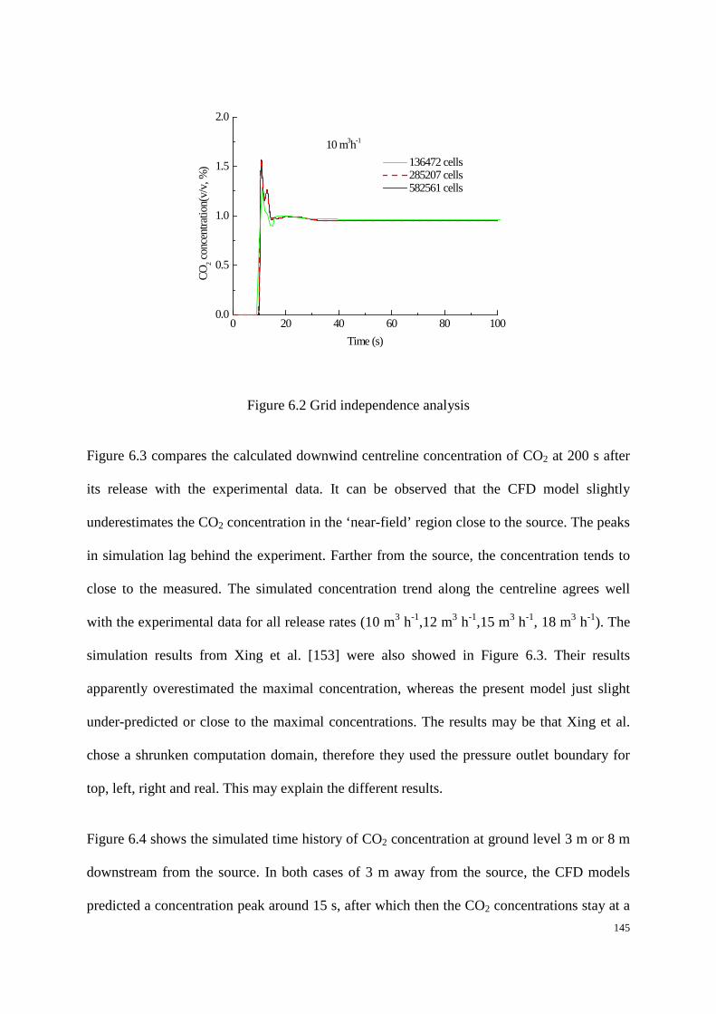
145

0 20 40 60 80 1000.0

0.5

1.0

1.5

2.0

136472 cells 285207 cells 582561 cells

CO2 c

once

ntra

tion(

v/v,

%)

Time (s)

10 m3h-1

Figure 6.2 Grid independence analysis

Figure 6.3 compares the calculated downwind centreline concentration of CO2 at 200 s after

its release with the experimental data. It can be observed that the CFD model slightly

underestimates the CO2 concentration in the ‘near-field’ region close to the source. The peaks

in simulation lag behind the experiment. Farther from the source, the concentration tends to

close to the measured. The simulated concentration trend along the centreline agrees well

with the experimental data for all release rates (10 m3 h-1,12 m3 h-1,15 m3 h-1, 18 m3 h-1). The

simulation results from Xing et al. [153] were also showed in Figure 6.3. Their results

apparently overestimated the maximal concentration, whereas the present model just slight

under-predicted or close to the maximal concentrations. The results may be that Xing et al.

chose a shrunken computation domain, therefore they used the pressure outlet boundary for

top, left, right and real. This may explain the different results.

Figure 6.4 shows the simulated time history of CO2 concentration at ground level 3 m or 8 m

downstream from the source. In both cases of 3 m away from the source, the CFD models

predicted a concentration peak around 15 s, after which then the CO2 concentrations stay at a

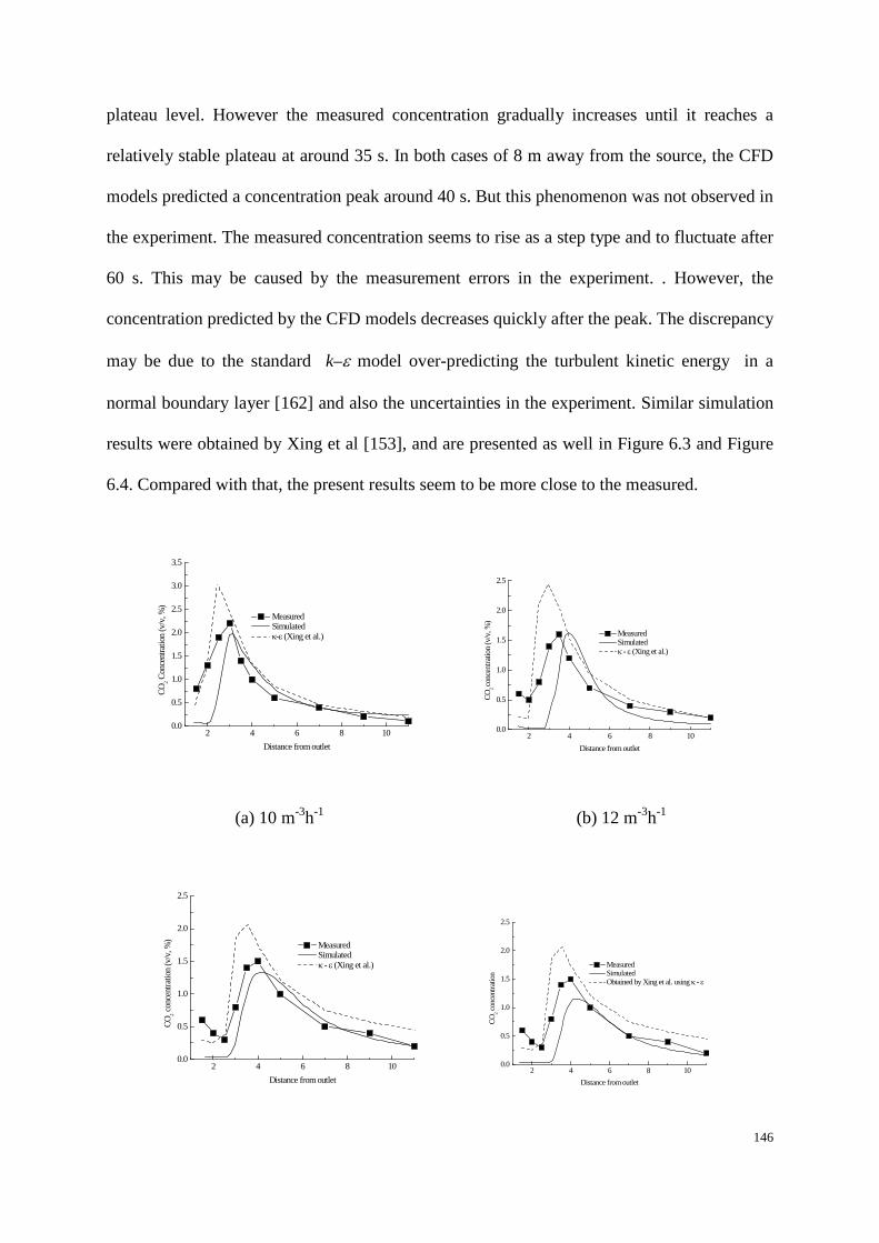
146

plateau level. However the measured concentration gradually increases until it reaches a

relatively stable plateau at around 35 s. In both cases of 8 m away from the source, the CFD

models predicted a concentration peak around 40 s. But this phenomenon was not observed in

the experiment. The measured concentration seems to rise as a step type and to fluctuate after

60 s. This may be caused by the measurement errors in the experiment. . However, the

concentration predicted by the CFD models decreases quickly after the peak. The discrepancy

may be due to the standard k–ε model over-predicting the turbulent kinetic energy in a

normal boundary layer [162] and also the uncertainties in the experiment. Similar simulation

results were obtained by Xing et al [153], and are presented as well in Figure 6.3 and Figure

6.4. Compared with that, the present results seem to be more close to the measured.

2 4 6 8 100.0

0.5

1.0

1.5

2.0

2.5

3.0

3.5

CO2 C

once

ntra

tion

(v/v

, %)

Distance from outlet

Measured Simulated κ-ε (Xing et al.)

2 4 6 8 100.0

0.5

1.0

1.5

2.0

2.5

CO2 co

ncen

tratio

n (v

/v, %

)

Distance from outlet

Measured Simulated κ - ε (Xing et al.)

(a) 10 m-3h-1 (b) 12 m-3h-1

2 4 6 8 100.0

0.5

1.0

1.5

2.0

2.5

CO2 co

ncen

tratio

n (v

/v, %

)

Distance from outlet

Measured Simulated κ - ε (Xing et al.)

2 4 6 8 100.0

0.5

1.0

1.5

2.0

2.5

CO2 co

ncen

tratio

n

Distance from outlet

Measured Simulated Obtained by Xing et al. using κ - ε

147

(c) 15 m-3h-1 (d) 18 m-3h-1

Figure 6.3 Ground level CO2 concentration along the centreline

0 20 40 60 80 1000.0

0.2

0.4

0.6

0.8

1.0

1.2

1.4

1.6

1.8

CO2 co

ncen

tratio

n (v

/v, %

)

Time (s)

Measured Simulated κ-ε (Xing et al.)

a. 10 m3h-1

0 20 40 60 80 1000.0

0.2

0.4

0.6

0.8

1.0

1.2

1.4

1.6

1.8

CO2 co

ncen

tratio

n (v

/v, %

)

Time (s)

Measured Simulated κ-ε (Xing et al.)

b. 12 m3h-1

(a) (4, 0, 0) (10 m-3h-1) (b) (4, 0, 0) (12 m-3h-1)

0 20 40 60 80 1000.0

0.2

0.4

0.6

CO2 co

ncen

tratio

n (v

/v, %

)

Time (s)

Measured Simulated κ-ε (Xing et al.)

c. 15 m3h-1

0 20 40 60 80 1000.0

0.2

0.4

0.6

CO2 co

ncen

tratio

n (v

/v, %

)

Time (s)

Measured Simulated κ-ε (Xing et al.)

d. 18 m3h-1

(c) (9, 0, 0) (15 m-3h-1) (d) (9, 0, 0) (18m-3h-1)

Figure 6.4 CO2 concentration time history at selected points – simulated vs measured

Although there are some discrepancies between the CFD predictions and experimental

measurements, the CFD models showed acceptable performance, especially in the far-field

region. The predicted concentration along the centreline has relatively good agreement with

the experimental data. This indicates that the proposed numerical methods can be used to

148

simulate the dispersion of CO2, particularly in the far-field region.

6.3.2 Simulation of Kit Fox experiment

The ‘Kit Fox’ field experiments of CO2 dispersion [163] were performed in 1995, at the

Frenchman Flat area of the Nevada Test Site, USA. The terrain texture was created using two

types of flat billboard-shaped roughness elements, strategically arranged to form an

‘Equivalent Roughness Pattern’ (ERP) and a ‘Uniform Roughness Array’ (URA). Figure 6.5

illustrates schematically the experimental arrangement, along with the locations of the

roughness elements and the measurement instrumentation.

Figure 6.5 Plan view of Kit Fox site

The ERP, including 75 thin, vertical billboards, each measuring 2.4 m squares, was installed

on the inner 39 m × 85 m rectangle, with a 1.5 m square CO2 source at ground level near the

centre of the ERP. The URA, which consists of 6,600 smaller rectangular billboards, was

installed on the outer 120 m × 314 m rectangle. In front of the URA, an array of 35 spires

was placed to reduce the distance required for development of the ABL. Concentration

sensors were installed on four arrays. Meteorological instruments were installed on five

Downrange (m)

Cros

sran

ge (m

)

-150 -100 -50 0 50 100 150 200 250120

90

60

30

-30

-60

-90

-120

0

Ground level source1.5 m x 1.5 m

Concentration monitor arrays 25 m, 50 m, 100 m, 225 m from source

"METn": METeorological towers with instruments

U R A

MET1

E R P

MET2

MET3 MET4

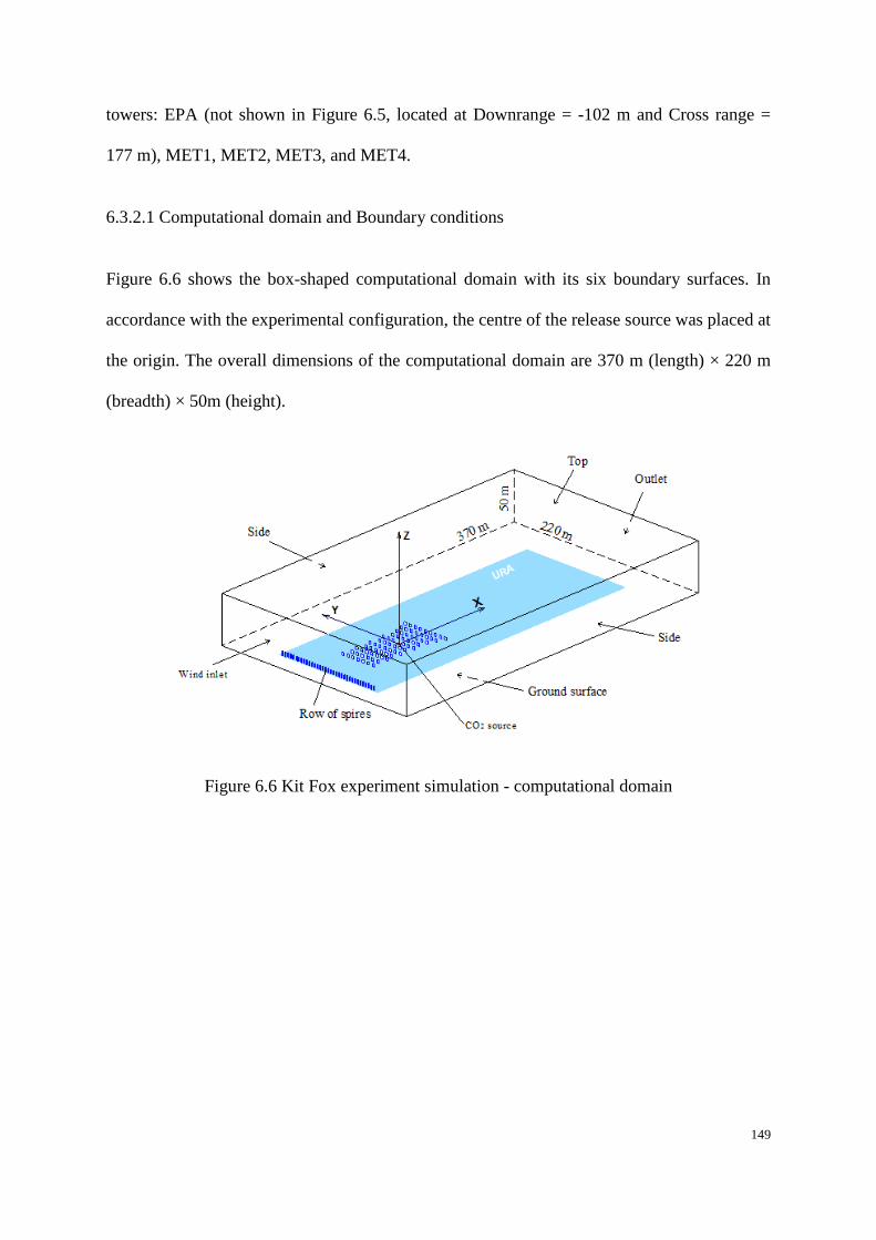
149

towers: EPA (not shown in Figure 6.5, located at Downrange = -102 m and Cross range =

177 m), MET1, MET2, MET3, and MET4.

6.3.2.1 Computational domain and Boundary conditions

Figure 6.6 shows the box-shaped computational domain with its six boundary surfaces. In

accordance with the experimental configuration, the centre of the release source was placed at

the origin. The overall dimensions of the computational domain are 370 m (length) × 220 m

(breadth) × 50m (height).

Figure 6.6 Kit Fox experiment simulation - computational domain

150

Figure 6.7 Computational mesh - details -

Both the ERP and spires had greatly small thickness but large surface area, which were

expected to have a significant influence on the flow behaviour close to the ground. In order to

retain these details in the computational domain and still meet the necessary mesh quality, the

ERP billboards and the spires were modelled as ‘baffles’, two-dimensional ‘surface bodies’

with zero thickness. The URA consisted of 6,600 much smaller elements, which could not be

represented individually. Instead, the area covered by the URA was represented by an

equivalent ‘rough wall’ with a specified roughness element dimension.

The computational domain was sub-divided into tetrahedral cells and was refined around the

ERP and the spires (Figure 6.7a). In this model, 10 ‘inflation’ layers were used to generate a

progressively finer computational mesh near the ground (Figure 6.7 b). The overall

computational grid contained 2.3 million cells, which enabled grid-independent simulations.

Seven boundary conditions were required (Figure 6.6): (1) CO2 inlet, (2) top, (3) outlet, (4)

left side, (5) right side, (6) wind inlet, and (7) ground. The CO2 inlet was specified by a mass

flow rate. The ‘top’ boundary was high enough and thus defined as an impermeable

151

‘symmetry’ boundary with zero normal velocity, gradients of all variables, and zero fluxes of

all quantities across it. The outlet was set as a pressure boundary with atmospheric pressure

(zero gauge pressure). The two side planes were defined as either wind velocity inlet or

pressure outlet, depending upon the mean wind direction. The wind inlet and ground

boundaries were carefully dealt with using the methods described in Section 6.3.1.

6.3.2.2 Simulation results and discussion

CFD simulations were carried out for all the continuous release trials of the Kit Fox

experiments, including 6 URA+ERP trials (with both URA and ERP in place) and 12 URA-

only trials (with only the URA in place). For (URA+ERP) cases, the CO2 release rate ranges

from 3.7 kg s-1 to 4 kg s-1, lasting from 120 s to 450 s, while for URA-only cases, the CO2

release rate ranges from 1.5 kg s-1 to 2 kg s-1, lasting from 120 s to 300 s.

Figure 6.8 Wind speed - simulation (—) vs measurement (■)

0 1 2 3 4 5 60

2

4

6

8

10

Hei

ght [

m]

0 1 2 3 4 5 60

2

4

6

8

10

0 1 2 3 4 5 60

2

4

6

8

10

Wind speed [m s-1]

Hei

ght [

m]

0 1 2 3 4 5 60

2

4

6

8

10

Wind speed [m s-1]

a. Trial 5-3 MET2 b. Trial 5-3 MET4

c. Trial 7-2 MET2 d. Trial 7-2 MET4

152

In all simulations, ambient mean wind velocity and temperature profiles were applied to the

relevant boundaries. It is important to ensure that the simulated wind velocity agrees well

with the experiment, so that the subsequent CO2 dispersion occurs in a correct environment.

Figure 6.8 compares the measured and simulated wind velocity profiles at MET2 and MET4

of trial 5-3 (URA+ERP) and trial 7-2 (URA-only). Clearly, the simulated wind velocity

profiles at MET2 agree very well with the measurements for both the (URA+ERP) and URA-

only cases. Despite the presence of the URA or the ERP upstream of MET4, which is 200 m

downstream of the inlet, the simulated far-field wind profiles there compare reasonably well

with experiment, as seen in Figure 6.8b and Figure 6.8d.

Figure 6.9 shows an overall view of the wind velocity vector field on a horizontal plane 1.2 m

from the ground in a (URA+ERP) case, along with a detail showing the wake that was

produced on the leeward sides of the obstacles (billboards). The wake flow is characterised

by flow recirculation regions, in which the released gas was trapped following its release at

the source and subsequent dispersion. This formed some new ‘sources’ that determine the

dispersion patterns further downstream. Correctly reflecting the flow behaviour in this region

is important for predicting the gas concentration field.

Figure 6.9 Plan view of wind velocity field and detail

Billboards

Wake flow

153

The experiments had four concentration monitor arrays located 25, 50, 100 and 225 m

downstream of the release point. Figure 6.10 compares the measured and simulated

downwind centreline concentration time histories at the different monitor arrays in trial 5-4

(URA+ERP) and trial 8-11 (URA-only). The overall performance of the CFD model is

satisfactory. There was reasonably good agreement between the simulated and experimental

results and the evolution of the CO2 concentration was captured reasonably accurately. The

CFD model tends to over-predict the CO2 concentration values, especially in the near-field

regions. This is possibly due to the application of the RANS model, which explicitly

separates the mean and the turbulent flow both in space and in time. Labovský & Jelemenský

[61] pointed out that using RANS to simulate a transient situation can only reflect long-term

variations and quick transients are not fully captured. The measured and predicted maximum

concentration values in the far-field region compare much better. Figure 6.10 also indicates

that when the dispersion parameters (gas release rate, wind velocity and temperature profiles)

are stable, the gas concentration at a specific downwind location tends to reach a steady value.

This may help quantitative estimation of the risk associated with the CO2 release.

154

Figure 6.10 CO2 concentration history - instantaneous concentration values

A comparative study was carried out between the CFD model and SLAB. The downwind

centreline CO2 concentration results calculated by SLAB were obtained from the Kit Fox

project report. Results for only 11 ‘continuous release’ trials have been reported. Table 6-2

compares the maximum 60 s average downwind CO2 concentrations predicted by the CFD

model and by SLAB, with the field measurements.

Table 6-2 CO2 concentration - measurement vs simulation (CFD and SLAB)

Trial 25 m 50 m 100 m 225 m

Expt CFD SLAB Expt CFD SLAB Expt CFD SLAB Expt CFD SLAB

3-5 15943 17782 34900 7604 7956 16200 5242 4419 7350 1975 2105 3175

4-4 40731 73950 83100 12333 16604 50900 7765 5974 12200 1958 2089 4020

5-3 9160 16924 22800 5565 6690 10230 2028 3560 4390 1112 1493 1560

5-4 9843 17396 24200 5435 6971 10960 3030 3878 4980 1413 1727 1860

0 50 100 150 200 2500

5000

10000

15000

20000a. Trial 5-4 Array 1

Conc

entra

tion

[ppm

]

0 100 200 3000

1000

2000

3000

4000

5000b. Trial 5-4 Array 3

0 100 200 3000

500

1000

1500

2000c. Trial 5-4 Array 4

0 100 200 300 400 5000

10000

20000

30000

40000

Time [s]

Conc

entra

tion

[ppm

]

d. Trial 8-11 Array 1

0 100 200 300 400 5000

2000

4000

6000

8000

Time [s]

e. Trial 8-11 Array 3

0 200 400 6000

1000

2000

3000

Time [s]

f. Trial 8-11 Array 4

Measurement CFD simulation

155

5-8 22482 26815 33600 12772 9030 16600 6675 4910 8070 2132 2534 2920

6-4 17026 29004 23300 6246 11704 8360 2435 4526 3350 1243 1355 755

6-6 34142 45341 35400 18594 19964 14100 9969 9079 5640 2993 2991 1850

6-9 35707 42696 32900 14281 18312 14100 8794 8248 5360 2950 3299 1620

7-9 37678 40846 31200 15201 18087 13500 7722 8390 5450 2701 3505 1850

7-12 64417 42813 36600 20068 18784 14500 9083 8545 6230 2912 3474 2300

8-8 15527 24056 23000 5970 9786 8350 2159 3909 2880 886 1264 782

Overall the CFD model is seen to perform much better than SLAB in (URA+ERP) cases

(from trial 3-5 to Trial 5-8 in Table 6-2). This may be due to the fact that SLAB was designed

for flat terrains, without the capability of modelling complex topographies/roughness patterns.

In case of URA-only trials (from trial 6-4 to trial 8-8), SLAB performs much better than

before, but to a large extent, it tends to under-predict the concentration values, while the CFD

model mostly produces slight over-predictions. Overall, the CFD model performs much

better than SLAB. SLAB can predict the measurements within a factor of 4, while the CFD

model can consistently keep the prediction within a factor of 2. Both SLAB and the CFD

model perform better in the far-field than in the near-field. In the far-field, the concentrations

predicted by the CFD model are very close to the experimental values.

Figure 6.11 compares graphically the measured and simulated downwind maximum

concentrations at the four monitor arrays for all cases. The dashed inclined lines enclose the

region for 0.67<Cp/Co<1.5 (Cp: predicted concentration; Co: observed concentration), while

the solid inclined lines enclose the region for 0.5<Cp/Co< 2. Clearly, the CFD model can keep

the relative prediction error within 50% for the URA-only cases. For URA+ERP cases, the

presence of the ERP brings considerable geometrical complexities into the computational

156

domain, but the model can consistently predict the measurements to within a factor of 2. The

single exception may be due to variation in the wind velocity and direction during the test.

Figure 6.11 CO2 concentration (10 s averaged value) - measurement vs simulation

A statistical methodology [88, 89] was employed to evaluate the performance of the CFD

model. The ‘performance measures’ include the Geometric Mean (MG), the Geometric

Variance (VG), the Fractional Bias (FB), the Normalised Mean Square Error (NMSE), and

the fraction of Cp within a FAC tor of 2 (FAC2) of Co. These performance measures are

defined as:

[ ])ln(expMG po CC= (6.14)

})][ln(exp{VG 2po CC= (6.15)

)()(2FB popo CCCC +−= (6.16)

)()(NMSE 2popo CCCC −= (6.17)

FAC2 = fraction of Cp within a factor of two of Co (6.18)

In Eq. (6.13) to (6.17), (¯) stands for the average over the data set.

100 1,000 10,000 100,000100

1,000

10,000

100,000

Measured concentration [ppm]

Pred

icte

d co

ncen

tratio

n [p

pm]

URA-only caseURA+ERP casedata3data4data5data6

157

A ‘perfect’ model would have MG=VG=FAC2=1, and FB=NMSE=0. While these values are

virtually impossible to achieve in reality because of the influence of random atmospheric

processes, a model with ‘acceptable’ performance has been defined as one that satisfies [89]:

1) FAC2 > 0.5; 2) -0.3 < FB < 0.3 or 0.7 < MG < 1.3; 3) NMSE < 4 or VG < 1.6.

Table 6-3 shows the performance measures of the CFD model. For comparison, performance

measures of the Gaussian model and SLAB, are also shown in Table 6-3. As the Gaussian

model was developed for flat terrains, its performance measures were based on the

predictions of 12 URA-only trials, using dispersion parameter formulae in Table 6-2 for an

open-country condition. The CFD model performs very well, with all measures close to the

‘perfect’ values. SLAB also fares well, with all performance measures within acceptable

thresholds. On the contrary, the performance of the Gaussian model is unacceptable: the

values of VG, FB, NMSE and FAC2 are all out of acceptable ranges.

Table 6-3 Model performance (CFD, Gaussian model, SLAB)

Model Data points MG VG FB NMSE FAC2

CFD 72 0.992 1.075 -0.018 0.106 0.986

Gaussian 48 1.228 2.318 -0.661 4.311 0.449

SLAB 72 0.831 1.306 -0.230 0.711 0.810

It should be noted that all the trials in the Kit Fox experiments were normal state, small-scale

CO2 releases. This is different from the real case of CO2 released from high-pressure

pipelines. However, simulations of these trials effectively validated the performance of the

CFD dispersion model using the proposed methods describing the ABL.

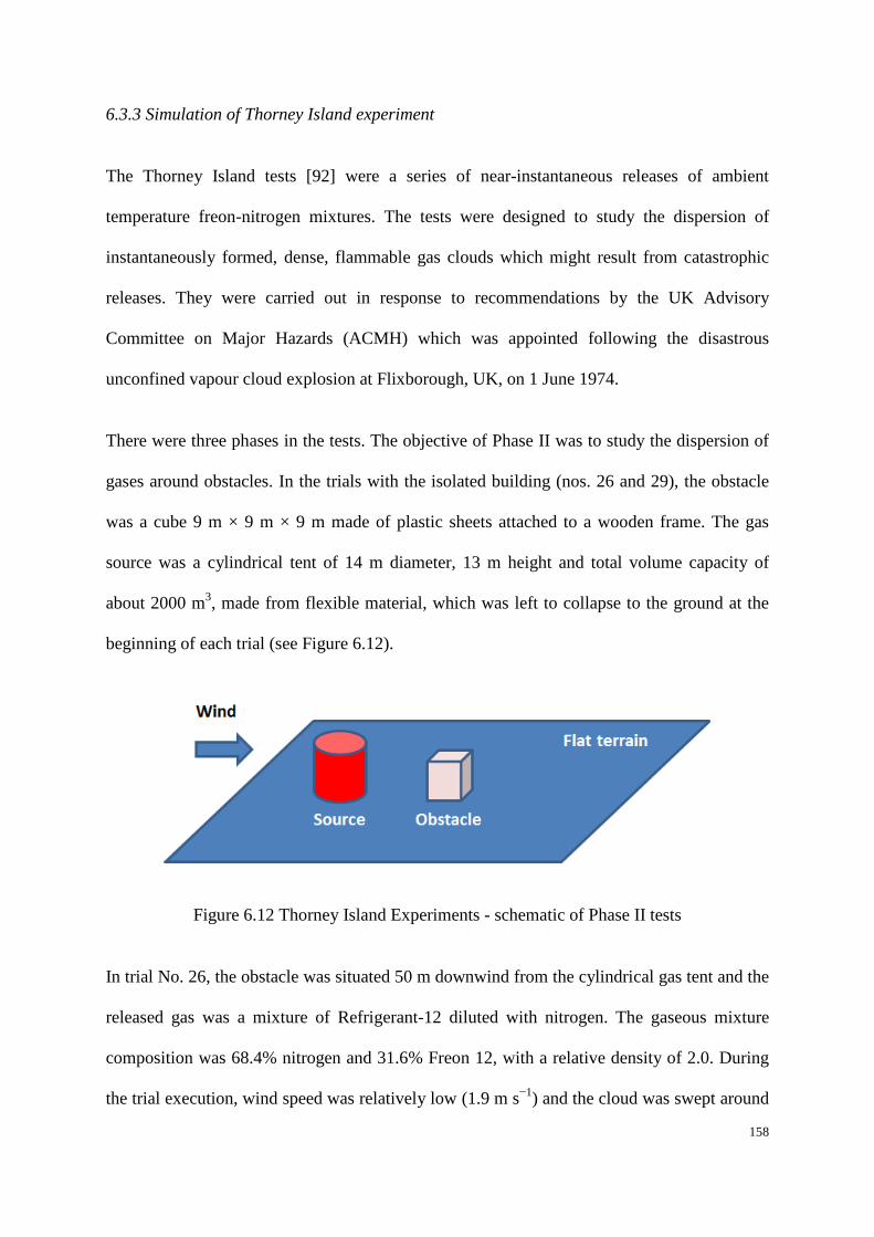
158

6.3.3 Simulation of Thorney Island experiment

The Thorney Island tests [92] were a series of near-instantaneous releases of ambient

temperature freon-nitrogen mixtures. The tests were designed to study the dispersion of

instantaneously formed, dense, flammable gas clouds which might result from catastrophic

releases. They were carried out in response to recommendations by the UK Advisory

Committee on Major Hazards (ACMH) which was appointed following the disastrous

unconfined vapour cloud explosion at Flixborough, UK, on 1 June 1974.

There were three phases in the tests. The objective of Phase II was to study the dispersion of

gases around obstacles. In the trials with the isolated building (nos. 26 and 29), the obstacle

was a cube 9 m × 9 m × 9 m made of plastic sheets attached to a wooden frame. The gas

source was a cylindrical tent of 14 m diameter, 13 m height and total volume capacity of

about 2000 m3, made from flexible material, which was left to collapse to the ground at the

beginning of each trial (see Figure 6.12).

Figure 6.12 Thorney Island Experiments - schematic of Phase II tests

In trial No. 26, the obstacle was situated 50 m downwind from the cylindrical gas tent and the

released gas was a mixture of Refrigerant-12 diluted with nitrogen. The gaseous mixture

composition was 68.4% nitrogen and 31.6% Freon 12, with a relative density of 2.0. During

the trial execution, wind speed was relatively low (1.9 m s−1) and the cloud was swept around

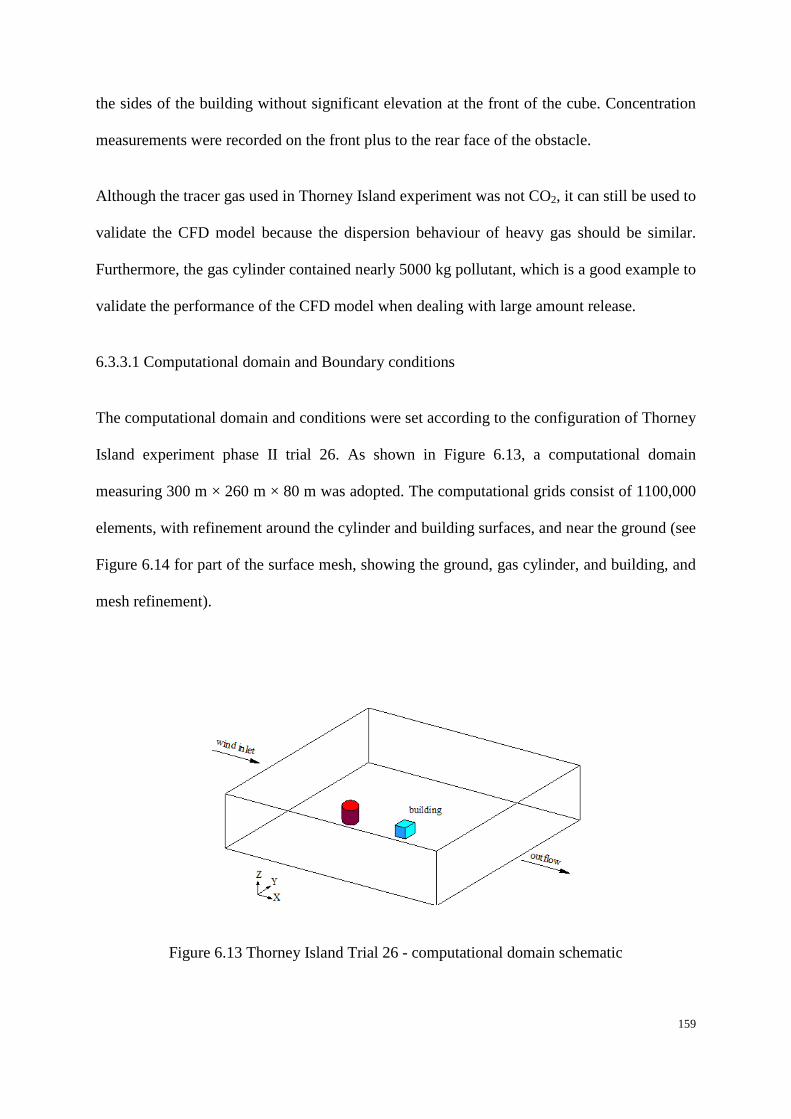
159

the sides of the building without significant elevation at the front of the cube. Concentration

measurements were recorded on the front plus to the rear face of the obstacle.

Although the tracer gas used in Thorney Island experiment was not CO2, it can still be used to

validate the CFD model because the dispersion behaviour of heavy gas should be similar.

Furthermore, the gas cylinder contained nearly 5000 kg pollutant, which is a good example to

validate the performance of the CFD model when dealing with large amount release.

6.3.3.1 Computational domain and Boundary conditions

The computational domain and conditions were set according to the configuration of Thorney

Island experiment phase II trial 26. As shown in Figure 6.13, a computational domain

measuring 300 m × 260 m × 80 m was adopted. The computational grids consist of 1100,000

elements, with refinement around the cylinder and building surfaces, and near the ground (see

Figure 6.14 for part of the surface mesh, showing the ground, gas cylinder, and building, and

mesh refinement).

Figure 6.13 Thorney Island Trial 26 - computational domain schematic

160

Figure 6.14 Thorney Island Trial 26 - surface mesh

Seven boundary conditions were required to be defined: (1) wind inlet, (2) ground, (3)

building surface, (4) left side, (5) right side, (6) top, (7) outlet, and (8) cylinder surface. The

velocity profile of the wind inlet, turbulence and ground roughness were specified using the

approaches mentioned above. The ground and building surface boundaries were defined as a

no-slip, isothermal wall with temperature equal to the ambient temperature. The ‘top’ and

two ‘side’ boundaries were defined as impermeable ‘symmetry’ boundaries. The outlet was

set as a pressure boundary with ambient pressure and temperature.

To imitate the rapid release of the pollutant source, at first the cylinder surface was set as a

no-slip wall and the initial condition of the flow field was obtained through a steady-state

simulation. After that, the cylinder surface was set as an interface which allows the fluid to go

through it freely and the transient simulation was carried out afterwards. The pollutant mass

contained in the cylinder was 4767 kg. The instantaneous release of it is equivalent to a

release with a mass flow rate of 3178 kg s-1, lasting 1.5 s [57].

6.3.3.2 Simulation results and discussion

After setting the conditions of the problem, a steady state case was initially solved to obtain

the initial values of the computational domain for the transient simulation. The convergence

161

criterion was set as the residual becoming equal or less than 10-4. Figure 6.15 shows the

resolved wind velocity distribution over the mid-plane of the domain. The wind velocity

profile at the inlet and the block effect of the building and the initial gas cylinder were well

reflected.

Figure 6.15 Steady-state wind velocity field in mid-plane

Figure 6.16 Steady-state streamline pattern in mid-plane

As shown in Figure 6.16, the flow recirculation patterns around the gas cylinder and the

building were well captured. This is important because it will greatly affect the initial

dispersion of the pollutant and also the gas dispersion behind the building.

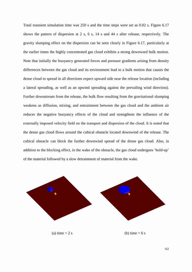
162

Total transient simulation time was 250 s and the time steps were set as 0.02 s. Figure 6.17

shows the pattern of dispersion at 2 s, 6 s, 14 s and 44 s after release, respectively. The

gravity slumping effect on the dispersion can be seen clearly in Figure 6.17, particularly at

the earlier times the highly concentrated gas cloud exhibits a strong downward bulk motion.

Note that initially the buoyancy generated forces and pressure gradients arising from density

differences between the gas cloud and its environment lead to a bulk motion that causes the

dense cloud to spread in all directions expect upward side near the release location (including

a lateral spreading, as well as an upwind spreading against the prevailing wind direction).

Further downstream from the release, the bulk flow resulting from the gravitational slumping

weakens as diffusion, mixing, and entrainment between the gas cloud and the ambient air

reduces the negative buoyancy effects of the cloud and strengthens the influence of the

externally imposed velocity field on the transport and dispersion of the cloud. It is noted that

the dense gas cloud flows around the cubical obstacle located downwind of the release. The

cubical obstacle can block the further downwind spread of the dense gas cloud. Also, in

addition to the blocking effect, in the wake of the obstacle, the gas cloud undergoes ‘hold-up’

of the material followed by a slow detrainment of material from the wake.

(a) time = 2 s

(b) time = 6 s

163

(c) time = 14 s

(d) time = 44 s

Figure 6.17 Evolution of gas cloud after collapse of pollutant container

(isosurface for 1% concentration)

There were two concentration sensors mounted on the building faces. One is on the windward

face at a height of 6.4 m, and another is on the leeward face at a height of 0.4 m. Figure 6.18

and 42 display a comparison between the measured and predicted gas concentration time

histories for windward and leeward faces respectively. The time histories of concentration

observed at the windward and leeward faces of the cubical obstacle are quite different. Note

that the persistence of the gas cloud (as measured by the difference between the arrival and

departure times of the cloud) observed at the leeward face of the cubical obstacle is

significantly greater than that observed at the windward face. This demonstrates the effect of

the obstacle on dispersion, where the recirculation in the wake region of the obstacle traps the

contaminant material of the gas cloud. The trapping of the pollutant within the wake of the

obstacle is correctly predicted by the model.

164

Figure 6.18 Pollutant concentration at 6.4 m elevation on windward side of obstacle

- simulation vs measurement -

Figure 6.19 Pollutant concentration at 0.4m elevation on leeward side of obstacle

- simulation vs measurement -

Generally, numerical predictions of concentration are seen to be in quite good agreement with

the experimental data. The trend of change in the concentrations on both the front and back

0 50 100 150 200 2500

0.02

0.04

0.06

0.08

Time (s)

Pollu

tant

con

cent

ratio

n (V

/V)

SimulatedMeasured

0 50 100 150 200 2500

0.005

0.01

0.015

0.02

0.025

Time (s)

Pollu

tant

con

cent

ratio

n (V

/V)

SimulatedMeasured

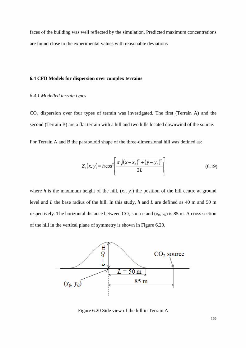
165

faces of the building was well reflected by the simulation. Predicted maximum concentrations

are found close to the experimental values with reasonable deviations

6.4 CFD Models for dispersion over complex terrains

6.4.1 Modelled terrain types

CO2 dispersion over four types of terrain was investigated. The first (Terrain A) and the

second (Terrain B) are a flat terrain with a hill and two hills located downwind of the source.

For Terrain A and B the paraboloid shape of the three-dimensional hill was defined as:

( ) ( ) ( )

−+−=

Lyyxx

hyxZs 2cos,

20

202 p

(6.19)

where h is the maximum height of the hill, (x0, y0) the position of the hill centre at ground

level and L the base radius of the hill. In this study, h and L are defined as 40 m and 50 m

respectively. The horizontal distance between CO2 source and (x0, y0) is 85 m. A cross section

of the hill in the vertical plane of symmetry is shown in Figure 6.20.

Figure 6.20 Side view of the hill in Terrain A

166

The third (Terrain B) mimics an urban area using box-shaped blocks to represent buildings.

The urban area for Terrain C is simply modelled using regular blocks to mimic buildings and

streets. The blocks are arranged in 4 rows and 4 columns, as shown in Figure 6.21. The

length and width of each building are 10 m and 8 m respectively. The height of all buildings

is varied in the simulations in order to assess its influence on the dispersion. The distance

between the centre of the CO2 source and the first row of buildings is 20 m. The space

between two buildings in the longitudinal direction is 10 m, while that in the lateral direction

is 8 m.

(a) Top view

(b) Side view

Figure 6.21 Top and side view of the urban area in Terrain B

1st row

3rd aisle 2nd aisle 1st aisle

Column 1

Column 2 Side longitudinal aisle

2nd row 3rd row 4th row

Central longitudinal aisle CO2 source

Wind

20 m

10 m

8 m

400 m 222 m

Wind

20 m 10 m

H

CO2 source

167

For the Terrain D, the topographic data was obtained using Google Maps. The grounds are

generated through these data using software Unigraphics NX as shown in Figure 6.22.

Figure 6.22 The topography of real terrain

6.4.2 Computational domain and Boundary conditions

Figure 6.23 gives the box-shaped computational domain for Terrain A. The overall

dimensions of the computational domain are 500 m (length) × 500 m (breadth) × 200 m

(height). The X-Y plane is placed on the ground, with the X-axis oriented along the wind.

CO2 is released vertically from a circular area source with a diameter of 1.5 m at ground level.

The mesh is refined near the CO2 source and ground. The total number of cells in the grid is

6306024 which is accurate enough for this dispersion (see Figure 6.24 for part of the

computational mesh of terrain A near the source and hill in computational symmetry).

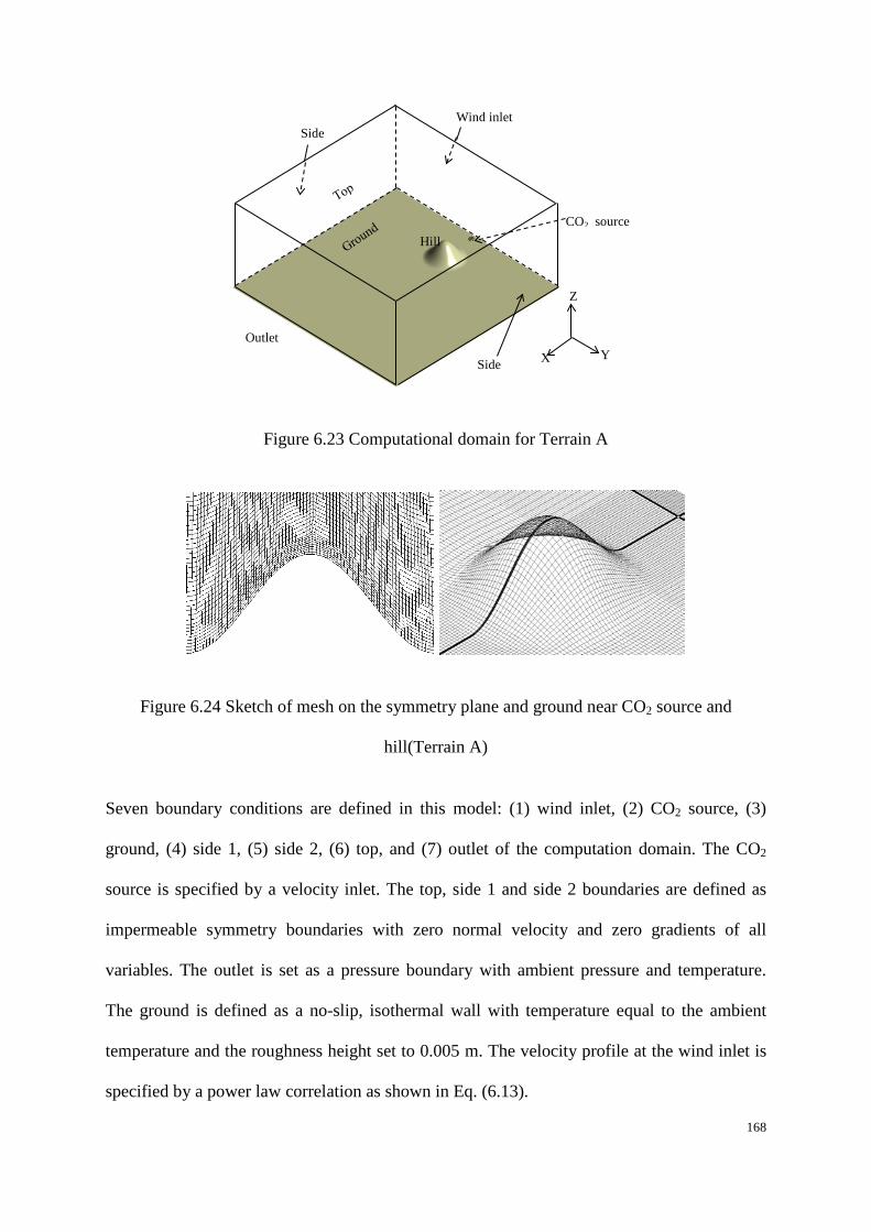
168

Figure 6.23 Computational domain for Terrain A

Figure 6.24 Sketch of mesh on the symmetry plane and ground near CO2 source and

hill(Terrain A)

Seven boundary conditions are defined in this model: (1) wind inlet, (2) CO2 source, (3)

ground, (4) side 1, (5) side 2, (6) top, and (7) outlet of the computation domain. The CO2

source is specified by a velocity inlet. The top, side 1 and side 2 boundaries are defined as

impermeable symmetry boundaries with zero normal velocity and zero gradients of all

variables. The outlet is set as a pressure boundary with ambient pressure and temperature.

The ground is defined as a no-slip, isothermal wall with temperature equal to the ambient

temperature and the roughness height set to 0.005 m. The velocity profile at the wind inlet is

specified by a power law correlation as shown in Eq. (6.13).

CO2 source

Wind inlet

Side

Outlet

Side

Z

X Y

Hill

169

The values of α = 0.1343, zr = 10 m in Eq. (6.13) are chosen in these simulations. Two

reference wind velocities, ur = 2 m s-1 and 6 m s-1，are chosen to study the influence of

weather conditions on the dispersion.

Figure 6.25 Typical mesh around a building for Terrain C

The boundary conditions for the CFD model simulating Terrain B, C and D are similar to

those for Terrain A. For Terrain C, the dimensions of the computational domain are 500 m

(length) × 500 m (breadth) × 200 m (height). The diameter of the CO2 source area is 0.5 m.

The number of cells in the computational domain ranges from 6.3 × 106 to 8.5 × 106 for

different building heights. A detail of the mesh around a typical building is shown in Figure

6.25.

Figure 6.26 shows the 3-D view of the box shape computational domain of the Terrain D

with its seven boundary surfaces. The overall dimensions of the computational space are 520

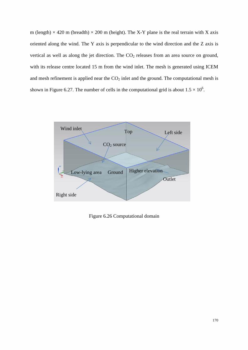
170

m (length) × 420 m (breadth) × 200 m (height). The X-Y plane is the real terrain with X axis

oriented along the wind. The Y axis is perpendicular to the wind direction and the Z axis is

vertical as well as along the jet direction. The CO2 releases from an area source on ground,

with its release centre located 15 m from the wind inlet. The mesh is generated using ICEM

and mesh refinement is applied near the CO2 inlet and the ground. The computational mesh is

shown in Figure 6.27. The number of cells in the computational grid is about 1.5 × 106.

Figure 6.26 Computational domain

CO2 source

Wind inlet

Right side

Ground Outlet

Top Left side

Higher elevation Low-lying area

171

Figure 6.27 Two-dimensional views of the computation mesh

6.4.3 Initial condition

Initially, a steady-state simulation was carried out to establish the wind flow field in the

computational domain. This provides the initial condition for the subsequent transient

simulations of CO2 dispersion. Figure 6.28 gives the simulated streamline pattern around the

hill in the symmetry plane. It is found that the streamline becomes sparse in the lee side of the

hill when the wind velocity is low and the recirculation in the lee side of the hill when the

wind velocity is relatively high, which corresponds to a relatively high Reynolds number..

This will provide an appropriate initial flow field for the subsequent dispersion simulation.

(a) Left side

(b) Right side

(c) Top view

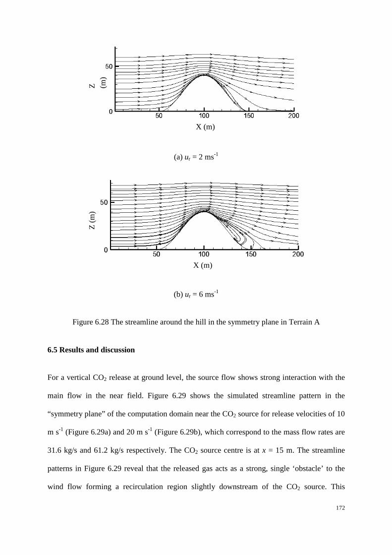
172

(a) ur = 2 ms-1

(b) ur = 6 ms-1

Figure 6.28 The streamline around the hill in the symmetry plane in Terrain A

6.5 Results and discussion

For a vertical CO2 release at ground level, the source flow shows strong interaction with the

main flow in the near field. Figure 6.29 shows the simulated streamline pattern in the

“symmetry plane” of the computation domain near the CO2 source for release velocities of 10

m s-1 (Figure 6.29a) and 20 m s-1 (Figure 6.29b), which correspond to the mass flow rates are

31.6 kg/s and 61.2 kg/s respectively. The CO2 source centre is at x = 15 m. The streamline

patterns in Figure 6.29 reveal that the released gas acts as a strong, single ‘obstacle’ to the

wind flow forming a recirculation region slightly downstream of the CO2 source. This

X (m)

Z (m)

Z (m

)

X (m)

173

phenomenon may influence the subsequent dispersion.

(a) vsource = 10 m s-1 (b) vsource = 20 m s-1

Figure 6.29 The streamline near the source

6.5.1 Simulation results - Terrain A

In the study of CO2 dispersion over Terrain A, 8 cases were simulated, considering four

source velocities and two wind velocities (see Table 6-4).

Table 6-4 The source strength and wind velocities of each case

Case vsource (m s-1) Mass flow

rate (kg/s) vwind (m s-1)

1 10 31.6 2

2 20 61.2 2

3 30 94.7 2

4 40 124.3 2

5 10 31.6 6

X (m) X (m)

Z (m

)

Z

174

6 20 61.2 6

7 30 94.7 6

8 40 124.3 6

The National Institute for Occupational Safety and Health (NIOSH) [126] suggests that an

exposure to CO2 concentration levels at 4% is immediately dangerous to life or health. The

Short-Term Exposure Limit (STEL) of 1.5% is used as a guide for maximum safe exposure.

This is the concentration below which no ill effect will be observed on people after a 15-

minute exposure [164], [165]. Figure 6.30, Figure 6.31 and Figure 6.33 show the simulation

results for vwind = 2 m s-1. Figure 6.30 shows the contours for CO2 concentration levels 4 %

(red contour) and 1.5 % (green contour) at ground level, 250 s after the release when the

dispersion is expected to approach a steady state. It is clear that in front of the hill (windward)

there exists a high CO2 concentration area due to the obstruction presented by the hill. But the

high concentration area seems to be smaller when the source velocity is increased high

enough that the CO2 cloud can rise over the hilltop. Given that CO2 is a heavier-than-air gas,

it has a natural tendency to sink during dispersion. For a vertical release with low initial

velocity, it is hard for CO2 to surmount the hill. Thus a large amount of the heavy gas will

accumulate on the windward side of the hill. Additionally the behaviour of the plume,

especially in presence of obstacles in the crosswind direction, seems to not be fully

symmetrical even though the symmetry geometry, due to the turbulent flow.

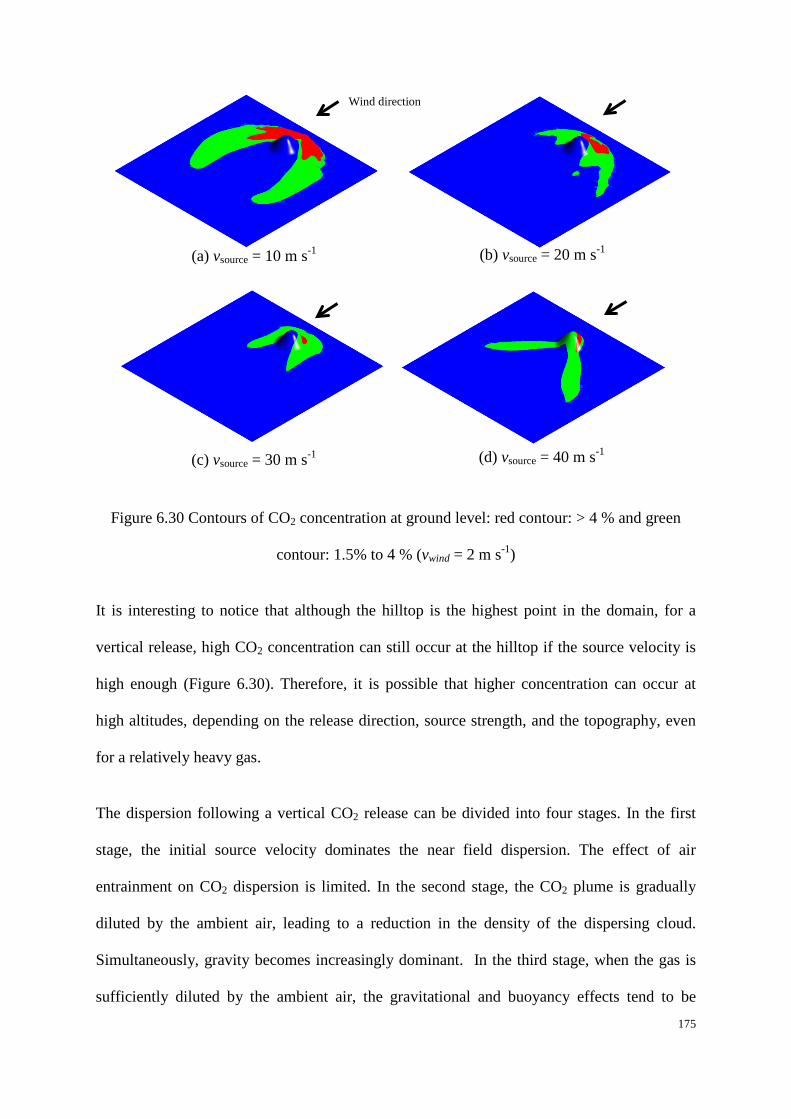
175

Figure 6.30 Contours of CO2 concentration at ground level: red contour: > 4 % and green

contour: 1.5% to 4 % (vwind = 2 m s-1)

It is interesting to notice that although the hilltop is the highest point in the domain, for a

vertical release, high CO2 concentration can still occur at the hilltop if the source velocity is

high enough (Figure 6.30). Therefore, it is possible that higher concentration can occur at

high altitudes, depending on the release direction, source strength, and the topography, even

for a relatively heavy gas.

The dispersion following a vertical CO2 release can be divided into four stages. In the first

stage, the initial source velocity dominates the near field dispersion. The effect of air

entrainment on CO2 dispersion is limited. In the second stage, the CO2 plume is gradually

diluted by the ambient air, leading to a reduction in the density of the dispersing cloud.

Simultaneously, gravity becomes increasingly dominant. In the third stage, when the gas is

sufficiently diluted by the ambient air, the gravitational and buoyancy effects tend to be

Wind direction

(a) vsource = 10 m s-1 (b) vsource = 20 m s-1

(c) vsource = 30 m s-1 (d) vsource = 40 m s-1

176

balanced. The CO2 cloud descends slightly even as it becomes bigger. In the fourth and final

stage, when the CO2 cloud is further diluted, the process approaches a condition which

represents a neutrally buoyant cloud. Then the gas becomes a passive contaminant. In the

third stage, if the CO2 cloud just reaches the hilltop, the concentration on the hill-top surface

will be extremely high.

Figure 6.31 The CO2 concentration contours on the ground at different times: red contour – >

4% and green contour – 1.5 - 4 % (vwind = 2 m s-1)

Figure 6.31 shows the CO2 concentration contours on the ground for case 1 and case 4 at

different times. For case 1, when the CO2 cloud encounters the hill, a part of the heavy gas

goes around the obstacle, and the remainder accumulates on the windward face of the hill.

For case 4, when the flow of CO2 encounters the obstacle, most of the heavy gas reaches the

hilltop. A small fraction goes around the hill, while the remainder accumulates on the

windward side of the hill. This makes the high concentration area around the hill to be

relatively smaller. This indicates that the terrain type and release velocity both have a

t = 50 s t = 100 s t = 150 s

(a) vsource = 10 m s-1

(b) vsource = 40 m s-1

Wind direction

177

combined influence on the dispersion of the heavy gas.

During the simulations, the concentration history was monitored at 4 points. As shown in

Figure 6.32, point A is located at the hill top, while point C is placed at the right side of the

hill. Point B and point D are located in the windward and leeward of the hill respectively.

Figure 6.33 gives the CO2 concentration time histories at these points for various release

velocities.

Figure 6.32 The diagram of the monitored point locations

A

B

C D

CO2 Source Wind

178

0 50 100 150 200 2500

1

2

3

4

5

6

CO 2 co

ncen

tratio

n (v

/v,%

)

Time (s)

(a) Concentration at Point A

0 50 100 150 200 2500123456789

101112

CO 2 co

ncen

tratio

n (v

/v,%

)

Time (s)

(b) Concentration at Point B

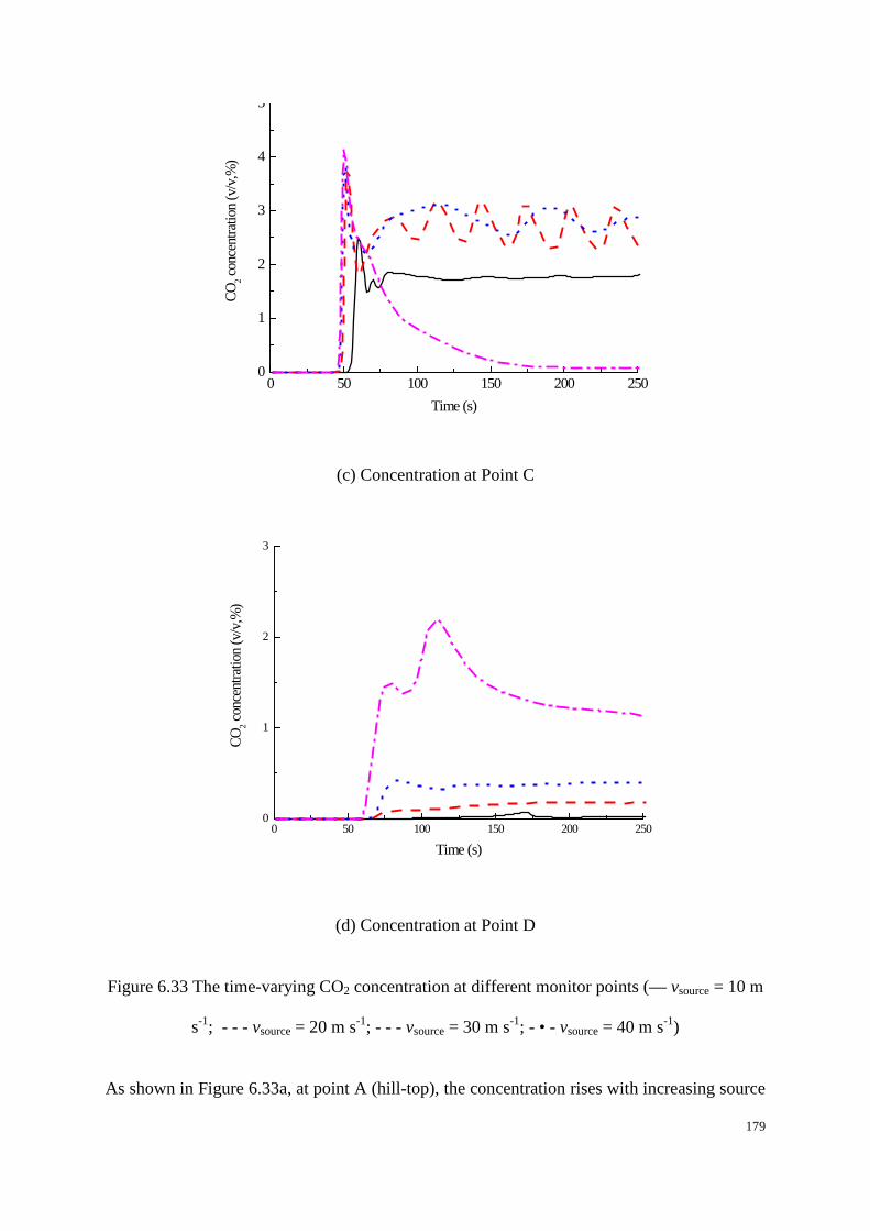
179

0 50 100 150 200 2500

1

2

3

4

5

CO 2 co

ncen

tratio

n (v

/v,%

)

Time (s)

(c) Concentration at Point C

0 50 100 150 200 2500

1

2

3

CO 2 co

ncen

tratio

n (v

/v,%

)

Time (s)

(d) Concentration at Point D

Figure 6.33 The time-varying CO2 concentration at different monitor points (— vsource = 10 m

s-1; - - - vsource = 20 m s-1; - - - vsource = 30 m s-1; - • - vsource = 40 m s-1)

As shown in Figure 6.33a, at point A (hill-top), the concentration rises with increasing source

180

velocity. The CO2 concentration is extremely low when vsource = 10 m s-1, and is much higher

for vsource = 40 m s-1 than for the other three release velocities. One reason is that the CO2

mass flow rate is high when vsource = 40 m s-1. The other reason is that when the vertical

source velocity is higher, the CO2 can surmount higher barriers or reach higher altitudes.

When the source velocity is relatively low, such as vsource = 10 m s-1, the CO2 cloud struggles

to reach the hill top. From Figure 6.33 we find that CO2 with 4 % concentration can reach the

hill-top only when vsource = 40 m s-1. When vsource = 10 m s-1, even CO2 with 1.5 %

concentration is not able to reach the hilltop.

As shown in Figure 6.33b, in cases 1, 2 and 3, the CO2 concentrations at point B (windward

face of the hill) are higher than those at the other three points. Especially when vsource = 10 m

s-1, the concentration nearly reaches 10 %. This indicates that the windward face of the hill is

the most likely to experience excessively high CO2 concentrations when CO2 cannot summit

the hill. Notice that when vsource = 40 m s-1, the concentration is relatively lower than other

leak velocities. The reason is that most of CO2 summits the hill.

As shown in Figure 6.33c, because of the blockage, CO2 tends to disperse around the hill. But

if the initial momentum of the source is high enough, the gas can also go over the hill top,

resulting in a lower concentration on the lateral sides of the hill. This is reflected in Figure

6.33c, while at point C (side of the hill), the CO2 concentration for vsource = 30 m s-1 is higher

than that for vsource = 40 m s-1.

As shown in Figure 6.33d, the CO2 concentrations at point D (leeward side of the hill) in all

four cases are lower than those at the other three points. This indicates that leeward of the hill

is the safest. Compared to the other three cases, the CO2 concentration for vsource = 10 m s-1 is

the lowest. This is due to the fact that the CO2 finds it harder to go across the hill with a lower

initial momentum, as most of the CO2 on the leeward side is made up of the part that has

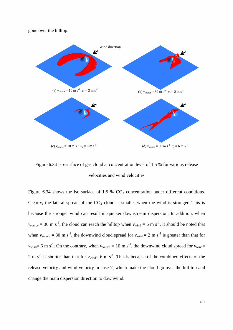
181

gone over the hilltop.

Figure 6.34 Iso-surface of gas cloud at concentration level of 1.5 % for various release

velocities and wind velocities

Figure 6.34 shows the iso-surface of 1.5 % CO2 concentration under different conditions.

Clearly, the lateral spread of the CO2 cloud is smaller when the wind is stronger. This is

because the stronger wind can result in quicker downstream dispersion. In addition, when

vsource = 30 m s-1, the cloud can reach the hilltop when vwind = 6 m s-1. It should be noted that

when vsource = 30 m s-1, the downwind cloud spread for vwind = 2 m s-1 is greater than that for

vwind= 6 m s-1. On the contrary, when vsource = 10 m s-1, the downwind cloud spread for vwind=

2 m s-1 is shorter than that for vwind= 6 m s-1. This is because of the combined effects of the

release velocity and wind velocity in case 7, which make the cloud go over the hill top and

change the main dispersion direction to downwind.

(a) vsource = 10 m s-1 ur = 2 m s-1 (b) vsource = 30 m s-1 ur = 2 m s-1

(c) vsource = 10 m s-1 ur = 6 m s-1 (d) vsource = 30 m s-1 ur = 6 m s-1

Wind direction

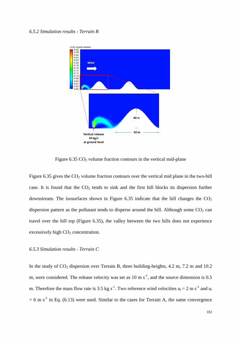
182

6.5.2 Simulation results - Terrain B

Figure 6.35 CO2 volume fraction contours in the vertical mid-plane

Figure 6.35 gives the CO2 volume fraction contours over the vertical mid plane in the two-hill

case. It is found that the CO2 tends to sink and the first hill blocks its dispersion further

downstream. The isosurfaces shown in Figure 6.35 indicate that the hill changes the CO2

dispersion pattern as the pollutant tends to disperse around the hill. Although some CO2 can

travel over the hill top (Figure 6.35), the valley between the two hills does not experience

excessively high CO2 concentration.

6.5.3 Simulation results - Terrain C

In the study of CO2 dispersion over Terrain B, three building-heights, 4.2 m, 7.2 m and 10.2

m, were considered. The release velocity was set as 10 m s-1, and the source dimension is 0.5

m. Therefore the mass flow rate is 3.5 kg s-1. Two reference wind velocities ur = 2 m s-1 and ur

= 6 m s-1 in Eq. (6.13) were used. Similar to the cases for Terrain A, the same convergence

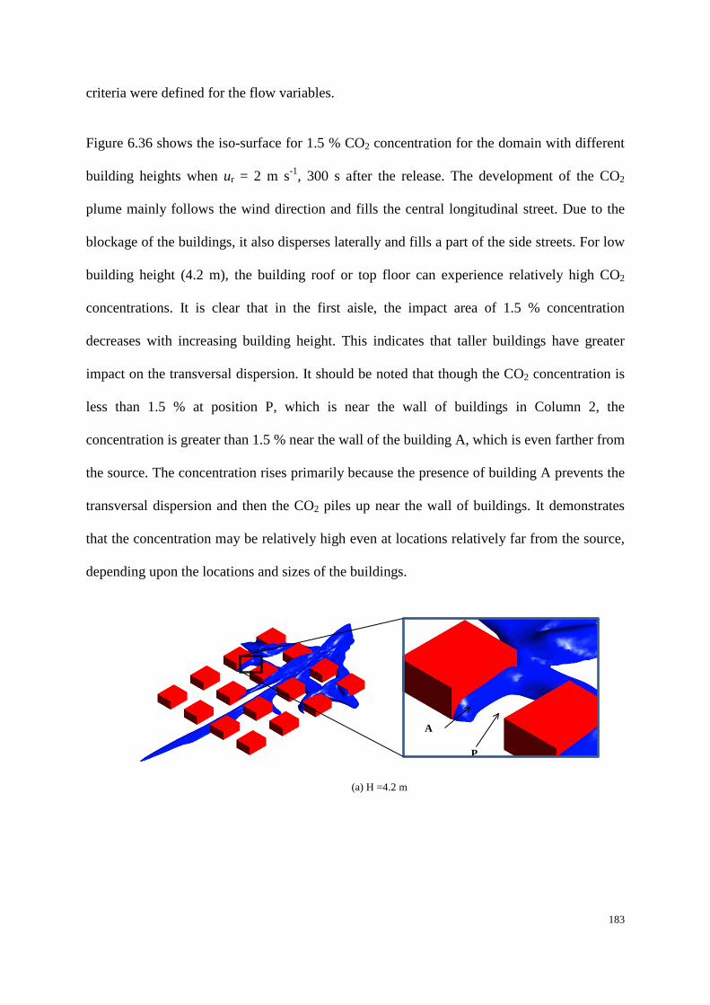
183

criteria were defined for the flow variables.

Figure 6.36 shows the iso-surface for 1.5 % CO2 concentration for the domain with different

building heights when ur = 2 m s-1, 300 s after the release. The development of the CO2

plume mainly follows the wind direction and fills the central longitudinal street. Due to the

blockage of the buildings, it also disperses laterally and fills a part of the side streets. For low

building height (4.2 m), the building roof or top floor can experience relatively high CO2

concentrations. It is clear that in the first aisle, the impact area of 1.5 % concentration

decreases with increasing building height. This indicates that taller buildings have greater

impact on the transversal dispersion. It should be noted that though the CO2 concentration is

less than 1.5 % at position P, which is near the wall of buildings in Column 2, the

concentration is greater than 1.5 % near the wall of the building A, which is even farther from

the source. The concentration rises primarily because the presence of building A prevents the

transversal dispersion and then the CO2 piles up near the wall of buildings. It demonstrates

that the concentration may be relatively high even at locations relatively far from the source,

depending upon the locations and sizes of the buildings.

P

A

(a) H =4.2 m

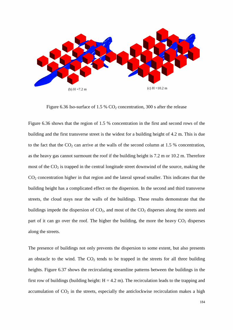
184

Figure 6.36 Iso-surface of 1.5 % CO2 concentration, 300 s after the release

Figure 6.36 shows that the region of 1.5 % concentration in the first and second rows of the

building and the first transverse street is the widest for a building height of 4.2 m. This is due

to the fact that the CO2 can arrive at the walls of the second column at 1.5 % concentration,

as the heavy gas cannot surmount the roof if the building height is 7.2 m or 10.2 m. Therefore

most of the CO2 is trapped in the central longitude street downwind of the source, making the

CO2 concentration higher in that region and the lateral spread smaller. This indicates that the

building height has a complicated effect on the dispersion. In the second and third transverse

streets, the cloud stays near the walls of the buildings. These results demonstrate that the

buildings impede the dispersion of CO2, and most of the CO2 disperses along the streets and

part of it can go over the roof. The higher the building, the more the heavy CO2 disperses

along the streets.

The presence of buildings not only prevents the dispersion to some extent, but also presents

an obstacle to the wind. The CO2 tends to be trapped in the streets for all three building

heights. Figure 6.37 shows the recirculating streamline patterns between the buildings in the

first row of buildings (building height: H = 4.2 m). The recirculation leads to the trapping and

accumulation of CO2 in the streets, especially the anticlockwise recirculation makes a high

(b) H =7.2 m (c) H =10.2 m

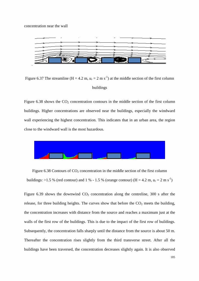
185

concentration near the wall

.

Figure 6.37 The streamline (H = 4.2 m, ur = 2 m s-1) at the middle section of the first column

buildings

Figure 6.38 shows the CO2 concentration contours in the middle section of the first column

buildings. Higher concentrations are observed near the buildings, especially the windward

wall experiencing the highest concentration. This indicates that in an urban area, the region

close to the windward wall is the most hazardous.

Figure 6.38 Contours of CO2 concentration in the middle section of the first column

buildings: >1.5 % (red contour) and 1 % - 1.5 % (orange contour) (H = 4.2 m, ur = 2 m s-1)

Figure 6.39 shows the downwind CO2 concentration along the centreline, 300 s after the

release, for three building heights. The curves show that before the CO2 meets the building,

the concentration increases with distance from the source and reaches a maximum just at the

walls of the first row of the buildings. This is due to the impact of the first row of buildings.

Subsequently, the concentration falls sharply until the distance from the source is about 50 m.

Thereafter the concentration rises slightly from the third transverse street. After all the

buildings have been traversed, the concentration decreases slightly again. It is also observed

186

that the building height affects the maximum downwind CO2 concentration. For a building

height of 4.2 m, the maximum CO2 concentration is the lowest. This is because in this case,

CO2 cloud more easy goes over the building roof and less CO2 accumulates in front of the

first row. When the building is high enough preventing the CO2 cloud from going across the

building roof, increasing the building height has little effect on the maximum concentration.

50 100 150 200 2500

2

4

6

8

10

12

14

CO2 c

once

ntra

tion

(v/v

, %)

Distance from the source (m)

H = 4.2 m H = 7.2 m H = 10.2 m

Figure 6.39 The maximum concentration (v/v, %) of CO2 along the downwind distance for

different building height

Figure 6.40 exhibits the relationship between the downwind distance from the CO2 source

and the concentration of CO2 at the centre of the ground for different wind conditions 300 s

after the release (H = 7.2 m). The concentration is higher when vwind= 2 m s-1.

187

50 100 150 200 2500

2

4

6

8

10

12

14

CO2 co

ncen

tratio

n (v

/v %

)

Distance from the source (m)

ur = 2 ms-1

ur = 6 ms-1

Figure 6.40 The maximum concentration (v/v, %) of CO2 along the downwind distance for

different weather condition

Figure 6.41 shows the influence of wind speed on the dispersion. It is clear that the spread of

the CO2 cloud decreases significantly – both in the lateral and longitudinal directions, for

higher wind speeds. This is similar to the simulation results of the dispersion over Terrain A

and B, which proves that a stronger wind helps the dispersion of CO2.

Figure 6.41 Isosurface of 1.5% CO2 concentration, 300 s after the release

a. ur = 2 m s-1 b. ur = 6 m s-1

188

6.5.4 Simulation results - Terrain D

Figure 6.42 CO2 concentration isosurfaces

In this simulation, reference wind velocity is 2 m s-1 at reference height 10 m. The CO2

source velocity is 10 ms-1 and mass flow rate is 3.51 kgs-1. Figure 6.42 shows the CO2

concentration isosurfaces over the real terrain 200 s after release. It indicates that CO2 tends

to flow more towards the low-lying area. Figure 6.43 shows the CO2 volume fraction over

vertical cross-sections at different distances downwind from the source. The difference in

elevation is clearly seen. Also, the welling up of CO2 in the low-lying area is likely to be due

to an updraft in the wind caused by the terrain.

Wind Wind

a) 15,000 ppm b) 1,500 ppm

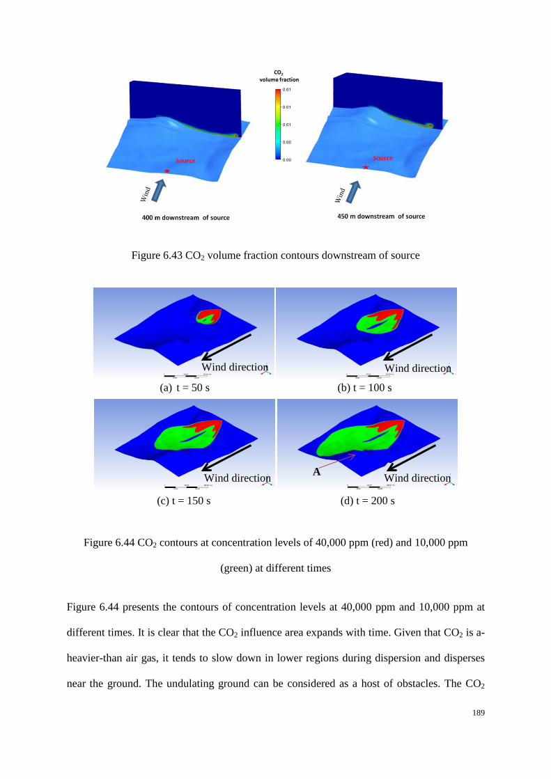
189

Figure 6.43 CO2 volume fraction contours downstream of source

Figure 6.44 CO2 contours at concentration levels of 40,000 ppm (red) and 10,000 ppm

(green) at different times

Figure 6.44 presents the contours of concentration levels at 40,000 ppm and 10,000 ppm at

different times. It is clear that the CO2 influence area expands with time. Given that CO2 is a-

heavier-than air gas, it tends to slow down in lower regions during dispersion and disperses

near the ground. The undulating ground can be considered as a host of obstacles. The CO2

(a) t = 50 s (b) t = 100 s

(d) t = 200 s (c) t = 150 s

Wind direction Wind direction

Wind direction Wind direction A

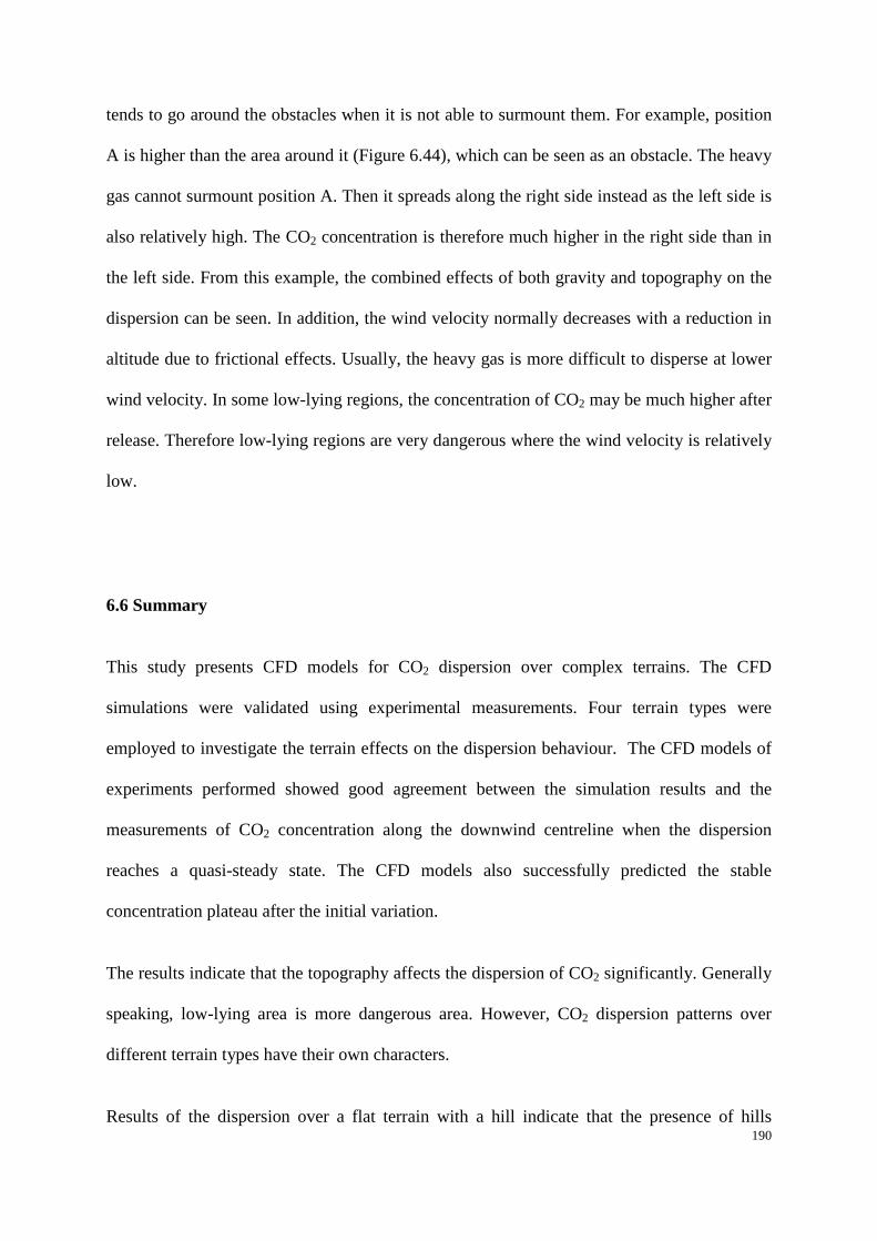
190

tends to go around the obstacles when it is not able to surmount them. For example, position

A is higher than the area around it (Figure 6.44), which can be seen as an obstacle. The heavy

gas cannot surmount position A. Then it spreads along the right side instead as the left side is

also relatively high. The CO2 concentration is therefore much higher in the right side than in

the left side. From this example, the combined effects of both gravity and topography on the

dispersion can be seen. In addition, the wind velocity normally decreases with a reduction in

altitude due to frictional effects. Usually, the heavy gas is more difficult to disperse at lower

wind velocity. In some low-lying regions, the concentration of CO2 may be much higher after

release. Therefore low-lying regions are very dangerous where the wind velocity is relatively

low.

6.6 Summary

This study presents CFD models for CO2 dispersion over complex terrains. The CFD

simulations were validated using experimental measurements. Four terrain types were

employed to investigate the terrain effects on the dispersion behaviour. The CFD models of

experiments performed showed good agreement between the simulation results and the

measurements of CO2 concentration along the downwind centreline when the dispersion

reaches a quasi-steady state. The CFD models also successfully predicted the stable

concentration plateau after the initial variation.

The results indicate that the topography affects the dispersion of CO2 significantly. Generally

speaking, low-lying area is more dangerous area. However, CO2 dispersion patterns over

different terrain types have their own characters.

Results of the dispersion over a flat terrain with a hill indicate that the presence of hills

191

downwind of the source may significantly shrink the spread of the CO2 cloud, especially

when the wind velocity is high. The downwind spread of the CO2 cloud is usually reduced by

the presence of the hill and the windward side of the hill experiences higher CO2

concentration. A part of the heavy gas goes around the hill, but for higher release velocity,

less CO2 spreads laterally. This makes the high concentration area around the hill to be

relatively smaller.

The terrain type and source strength have a combined effect on the dispersion of CO2. For

vertical releases, high CO2 concentration can occur at the hilltop if the source velocity is high

enough, because the source strength and wind velocity can help the cloud spread to higher

altitudes. The leeward of the hill is the safest due to the fact that the CO2 finds it harder to go

across the hill, as most of the CO2 on the leeward side is made up of the part that has gone

over the hilltop.

Results of the dispersion over a flat terrain with two hills indicate that the hill changes the

CO2 dispersion pattern as the pollutant tends to disperse around the hill.

In an urban area, the CO2 cloud is usually trapped in the streets between buildings. In the

streets, it is more dangerous near the wall, especially near the windward wall. The coverage

of hazardous area increases with the decrease of building height, as higher buildings lead to

less lateral spread of the CO2 cloud. Higher buildings may lead to higher ground-level

maximum CO2 concentration. But when the building is high enough preventing the CO2

cloud from going over the building roof, increasing the building height has little effect on the

maximum CO2 concentration.

Strong wind contributes to the dispersion. This was shown in the CO2 dispersion over terrain

types. Higher wind velocity leads to quicker dispersion, resulting in a smaller impact area.

192

Results of the dispersion over a real terrain show that, in some low-lying regions, the

concentration of CO2 may be much higher after release.

193

Chapter 7 Study of the consequence of CO2 released from high-

pressure pipeline

194

In this study, a “whole model” involving CO2 released from a high-pressure pipeline is

presented. The “whole model” includes predictions of discharge rate, atmospheric expansion

and dispersion. A multi-phase Computational Fluid Dynamics (CFD) model is presented to

simulate CO2 releases from high-pressure pipelines. A real gas EOS, the GERG-2008 EOS,

was incorporated into the CFD code, which was used in discharge and expansion models.

This can ensure more accurate prediction of “source strength”. The influences of non-

equilibrium phase transition, stagnation conditions, pipeline parameters, and weather

conditions on dispersion will be discussed.

7.1 Introduction

As described in Section 1.2, after the release of CO2 from a high pressure pipeline, a region of

two-phase flow can be initiated in the pipe by rapid depressurisation. Following the release,

the fluid expands to ambient pressure as an under-expanded jet. During the jet, CO2 may

experience cooling down rapidly and de-sublimation due to the Joule-Thomson effect [6]. As

a heavier-than air gas, CO2 tends to slump to the ground. After travelling for a certain

distance, the cloud will lose its initial momentum and be effectively mixed with air, and

disperse as a “Gaussian” cloud.

Apart from an appropriate dispersion model, the precision of prediction of the CO2 release

from the high pressure pipeline requires a precise model for source strength; it is crucial for

the prediction of dispersion following a CO2 release. Therefore efforts have been made to

develop appropriate CO2 pipeline discharge rates, such as Wilson’s method [84], Morrow

model [85] and Phast modules [87]. However, the equations in these models over-simplify

the physical phenomenon of the discharge process; therefore they cannot obtain the source

195

strength accurately. Later, a number of researchers [9-11] used one-dimensional transient

Navier-Stokes mass, momentum, and energy balance equations expressed in terms of fluid

velocity, density, and pressure, in conjunction with a ‘real gas’ Equation of State (EOS) to

predict the discharge process. In the above models, the fluid is considered to remain at

thermal and mechanical equilibrium during depressurisation, with possible non-equilibrium

phase transition ignored. As mentioned in Section 2.2, this assumption may generate

discrepancy. In addition, the predictions of properties obtained by PR EOS are not accurate

enough for liquid CO2. The non-equilibrium liquid/vapour transition probably affects the

prediction of the heavy gas dispersion. In this study, in order to develop a better

understanding of the phase transition during the depressurisation of a high-pressure CO2

release and consequently help the source strength prediction, a multi-phase CFD model is

proposed. The GERG-2008 EOS was incorporated into the CFD code to give precise physics

property estimations for both liquid and vapour phases. The phase transition was modelled by

considering the inter-phase mass transfer and the latent heat due to vaporisation. The results

from the decompression mode provide the inlet conditions for the following heavy gas

dispersion model. The effects of non-equilibrium phase transition, stagnation conditions,

pipeline parameters, impurity/impurities on discharge rate and dispersion will be discussed.

7.2 Methodology

7.2.1 Definition of the problem

As mentioned in Chapter 1, the whole process can be divided into 3 parts - Decompression,

Expansion and Dispersion. In terms of Decompression and Expansion, the mesh requirement

for predicting highly transient high-speed flow is dense and the requirement of time step is

short. However, dispersion modelling requires a large enough domain to allow the spread of

dense gas without the results being adversely affected by the boundary condition. Therefore,

196

an overall CFD model including both the depressurisation and dispersion domains would be

unacceptably time-consuming. Thus, each part will be studied separately, as shown in Figure

1.3.

The Depressurisation part is to obtain the flow conditions at the Exit (Pe, ρe and ue ect.). For

conservation prediction, a full-bore rupture at one end of the pipeline is considered. In this

part, only the flow inside the pipe is considered. For a real pipeline, the fluid will continue to

flow into the pipe after the rupture has occurred until an isolation valve is closed. For

simplicity, in this study the fluid is assumed to be initially at rest, with the pipeline closed at

one end and suddenly opened at the other. The Expansion part is to determine the jet flow

conditions at ambient pressure by using the source strength at Exit. The values of jet flow

conditions allow to be used as inlet boundary conditions for the Dispersion part. In this study,

simulations of depressurisation and dispersion were carried out using the commercial CFD

code ANSYS-Fluent. The under-expanded expansion was modelled by simplified,

conservation equations to avoid resolving the high pressure gradients.

7.2.2 Depressurisation model

As described in Chapters 2, 3 and 4, the non-equilibrium effect on pipe-flow should not be

overlooked. Therefore the depressurisation model considers the non-equilibrium effect. The

methodology for depressurisation is the same as the multi-phase decompression model in

Chapter 3 and 4. In this study, a one-dimension mesh was employed to minimise the

computing time, which was schematically shown in Figure 7.1. The lengths of computation

domains were from 1 km to 5 km. The “symmetry” boundary was applied to the two lateral

sides. An ambient pressure boundary was used at the pipe exit. The pipe closed end was

defined as a no-slip wall. Close to the exit, within 100 m, the width of the element is 0.01 m,

while it gradually increases to 0.1 m afterwards.

197

It should be noted that friction is neglected in the one-dimensional model. This simplification

will lead to over-prediction of the source strength. However for risk assessment, a

conservative prediction is usually acceptable.

Figure 7.1 Schematic of full bore rupture simulation computational mesh

7.2.3 Expansion model

After exiting from the rupture opening, the flow presents as an under-expanded jet with very

high momentum and reaches ambient pressure very soon. In this work, the model used by

DNV phast was employed. Phast is a hazard analysis software tool, which provides an

ATmospheric EXpansion module ATEX [87] to deal with the expansion of a continuous

release from the conditions in the leak rupture opening down to atmospheric pressure. The

basic equations in ATEX can be found in Section 2.4, from Eqs. (2.59) – (2.64) The density

and enthalpy are estimated using GERG-2008 EOS.

7.2.4 Dispersion model

In order to obtain conservative predictions and remove the uncertainties of considering dry

ice sublimation, an “all-gas” model is used to predict the consequence distance. Figure 7.2

shows the scheme of the box-shaped computational domain for the dispersion model. The

overall dimensions of the computational domain are 1000 m (X) × 400 m (Y) × 200 m (Z).

The computational domain is discretised in the form of hexahedral cells. The mesh is refined

near the CO2 source and ground. The total number of cells is approximately 2.5 million

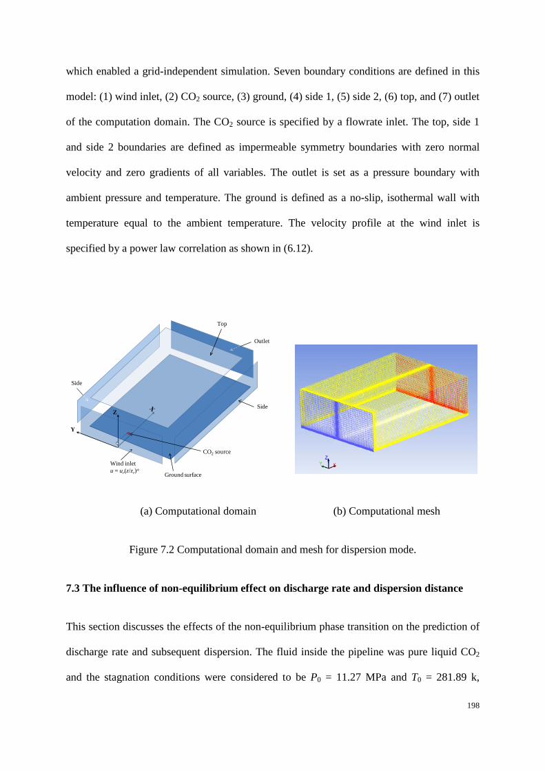
198

which enabled a grid-independent simulation. Seven boundary conditions are defined in this

model: (1) wind inlet, (2) CO2 source, (3) ground, (4) side 1, (5) side 2, (6) top, and (7) outlet

of the computation domain. The CO2 source is specified by a flowrate inlet. The top, side 1

and side 2 boundaries are defined as impermeable symmetry boundaries with zero normal

velocity and zero gradients of all variables. The outlet is set as a pressure boundary with

ambient pressure and temperature. The ground is defined as a no-slip, isothermal wall with

temperature equal to the ambient temperature. The velocity profile at the wind inlet is

specified by a power law correlation as shown in (6.12).

(a) Computational domain (b) Computational mesh

Figure 7.2 Computational domain and mesh for dispersion mode.

7.3 The influence of non-equilibrium effect on discharge rate and dispersion distance

This section discusses the effects of the non-equilibrium phase transition on the prediction of

discharge rate and subsequent dispersion. The fluid inside the pipeline was pure liquid CO2

and the stagnation conditions were considered to be P0 = 11.27 MPa and T0 = 281.89 k,

Outlet

Top

Side

Side

Ground surface

Wind inletu = ur(z/zr)α

CO2 source

Y

Z

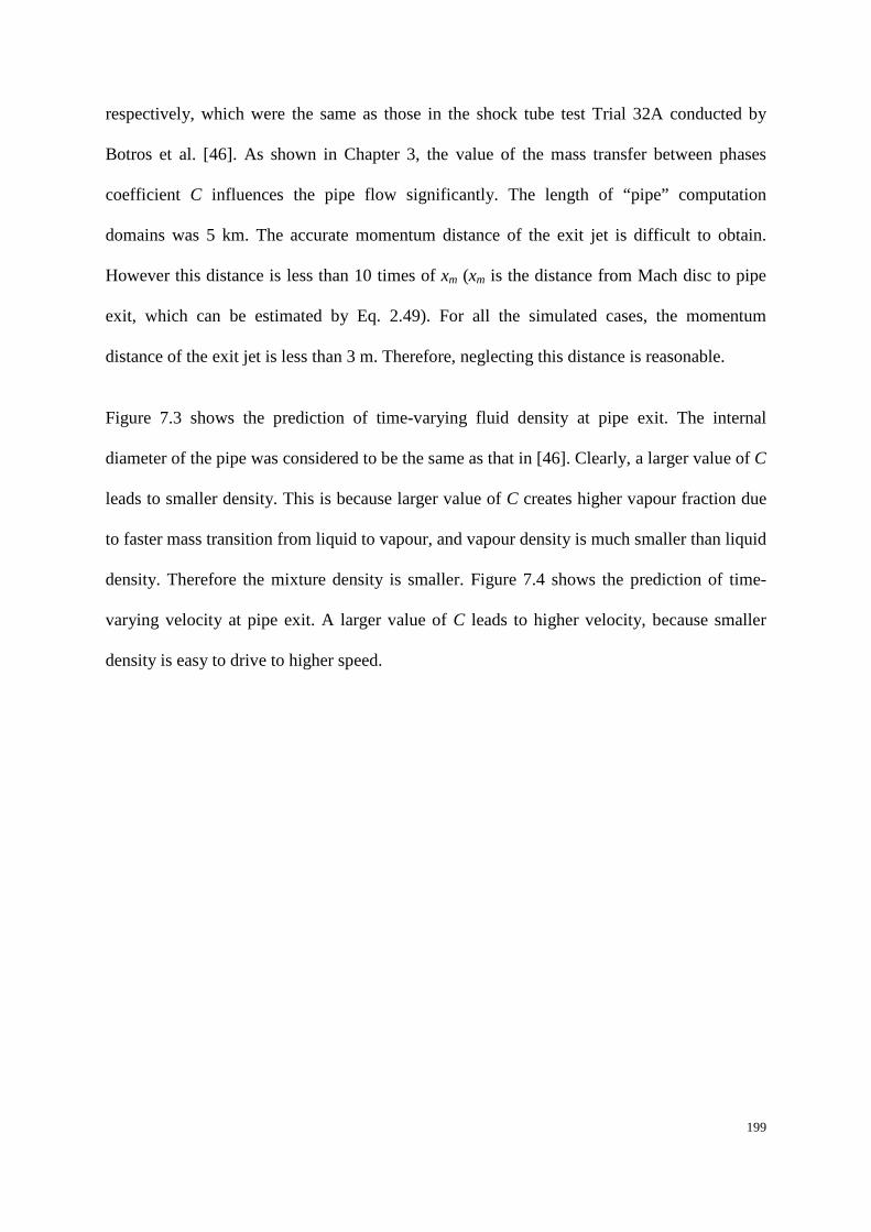
199

respectively, which were the same as those in the shock tube test Trial 32A conducted by

Botros et al. [46]. As shown in Chapter 3, the value of the mass transfer between phases

coefficient C influences the pipe flow significantly. The length of “pipe” computation

domains was 5 km. The accurate momentum distance of the exit jet is difficult to obtain.

However this distance is less than 10 times of xm (xm is the distance from Mach disc to pipe

exit, which can be estimated by Eq. 2.49). For all the simulated cases, the momentum

distance of the exit jet is less than 3 m. Therefore, neglecting this distance is reasonable.

Figure 7.3 shows the prediction of time-varying fluid density at pipe exit. The internal

diameter of the pipe was considered to be the same as that in [46]. Clearly, a larger value of C

leads to smaller density. This is because larger value of C creates higher vapour fraction due

to faster mass transition from liquid to vapour, and vapour density is much smaller than liquid

density. Therefore the mixture density is smaller. Figure 7.4 shows the prediction of time-

varying velocity at pipe exit. A larger value of C leads to higher velocity, because smaller

density is easy to drive to higher speed.

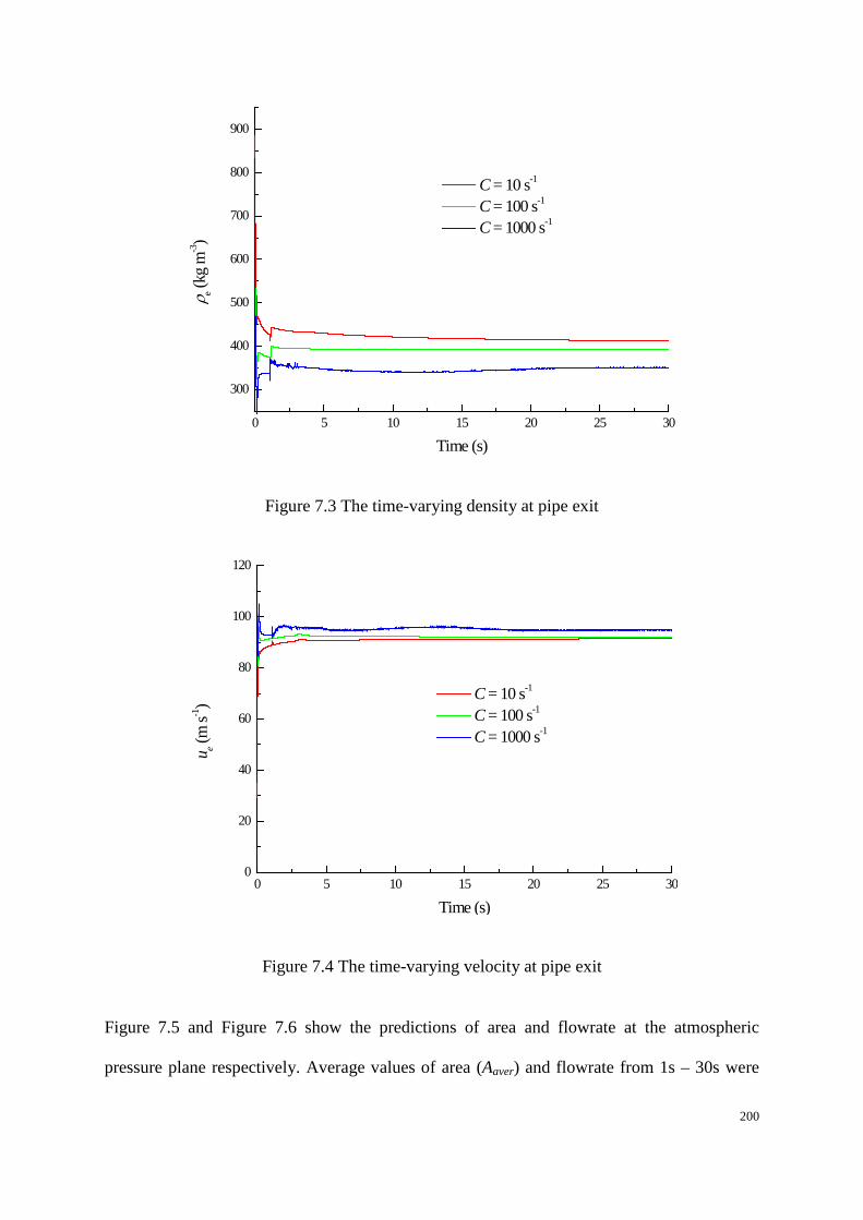
200

0 5 10 15 20 25 30

300

400

500

600

700

800

900

ρ e (kg

m-3)

Time (s)

C = 10 s-1

C = 100 s-1

C = 1000 s-1

Figure 7.3 The time-varying density at pipe exit

0 5 10 15 20 25 300

20

40

60

80

100

120

u e (m

s-1)

Time (s)

C = 10 s-1

C = 100 s-1

C = 1000 s-1

Figure 7.4 The time-varying velocity at pipe exit

Figure 7.5 and Figure 7.6 show the predictions of area and flowrate at the atmospheric

pressure plane respectively. Average values of area (Aaver) and flowrate from 1s – 30s were

201

used as the CO2 source conditions for dispersion following, which are shown as

corresponding solid lines. Clearly, a larger value of C leads to smaller Aaver and lower average

flowrate.

0 5 10 15 20 25 300.00

0.05

0.10

0.15

0.20

0.25

0.30

0.35

A a (m2 )

Time (s)

C = 10 s-1 C = 100 s-1

C = 1000 s-1

Figure 7.5 The time-varying area at atmospheric pressure plane

202

0 5 10 15 20 25 300

10

20

30

40

50

Flow

rate

(kg

s-1)

Time (s)

C = 10 s-1

C = 100 s-1

C = 1000 s-1

Figure 7.6 The time-varying velocity at atmospheric pressure plane

Figure 7.7 shows the predicted consequence distances of 10% following full-bore rupture of a

CO2 pipeline after 150 s release, when the dispersion is expected to approach a steady state.

The wind velocity of ur is set as 6 m/s in Eq. (9) for this simulation. Clearly, a larger value of

C predicted the consequence distance a little shorter than that predicted by smaller value of C,

because a larger value of C creates a lower flowrate. This indicates that under-estimation of

non-equilibrium phase transition in the pipe leads to under-prediction of the consequence

distance.

Figure 7.7 Hazardous cloud of 10% CO2 concentration predicted by different values of C (top

view)

25.0 m

C = 10 s-1

23.5 m

C = 100 s-1

21.1 m

C = 1000 s-1

203

7.4 The influences of initial pressure, wind velocity and pipe diameters on discharge

rate and dispersion distance

For a real pipeline, the distance between isolation valves is usually several dozen kilometres.

Therefore, the length from rupture to isolation valve or pipe end may be very long. To avoid

unrealistic time-consuming, in this study, a 5 km long pipeline subjected to a full-bore

rupture at one end is considered in this simulation. The expression of the source strength and

a function of time will be discussed. The stagnation conditions and were also considered the

same as in the shock tube test Trial 32A [69]. As studied above, C = 10 s-1 seems to be the

optimum value for pure CO2 at a range of pressure in terms of temperature about 280 k. Thus,

C = 10 s-1 is used in the following simulation.

In Figure 7.8 the consequence distances predicted using reference wind velocities of 2 m s-1

and 6 m s-1 are compared. In this study, the pipe internal diameter (ID) is 38.1 mm.

According to the results, a higher wind velocity leads to a longer consequence distance, but

the influence of wind speed is insignificant. It is true that high wind speed contributes to the

dispersion as increasing the wind speed improves transport and mixing. However, when

horizontal releases become large with high momentum, the dispersion tends to be dominated

by the source momentum. Therefore, the wind probably drives the CO2 cloud further

downstream in terms of large horizontal releases. Consequently, a higher wind velocity may

result in longer consequence distances. It should be noted that the impact created by wind

velocity is small, because compared with that of CO2 discharge velocity, the wind velocity is

considerably lower. When the wind velocity is increased from 6 m s-1 to 2 m s-1, the CO2

concentration envelope can be shrunk about 0.4 m. This indicates that the wind has different

effects on different release directions.

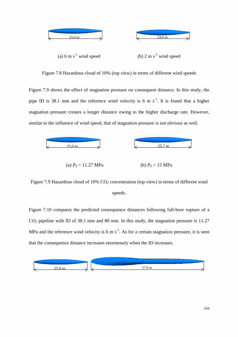
204

(a) 6 m s-1 wind speed (b) 2 m s-1 wind speed

Figure 7.8 Hazardous cloud of 10% (top view) in terms of different wind speeds

Figure 7.9 shows the effect of stagnation pressure on consequent distance. In this study, the

pipe ID is 38.1 mm and the reference wind velocity is 6 m s-1. It is found that a higher

stagnation pressure creates a longer distance owing to the higher discharge rate. However,

similar to the influence of wind speed, that of stagnation pressure is not obvious as well.

(a) P0 = 11.27 MPa (b) P0 = 15 MPa

Figure 7.9 Hazardous cloud of 10% CO2 concentration (top view) in terms of different wind

speeds.

Figure 7.10 compares the predicted consequence distances following full-bore rupture of a

CO2 pipeline with ID of 38.1 mm and 80 mm. In this study, the stagnation pressure is 11.27

MPa and the reference wind velocity is 6 m s-1. As for a certain stagnation pressure, it is seen

that the consequence distance increases enormously when the ID increases.

25.0 m 24.6 m

25.0 m 25.7 m

25.0 m 57.6 m

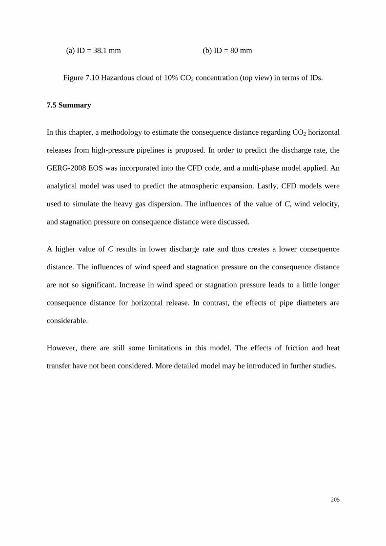
205

(a) ID = 38.1 mm (b) ID = 80 mm

Figure 7.10 Hazardous cloud of 10% CO2 concentration (top view) in terms of IDs.

7.5 Summary

In this chapter, a methodology to estimate the consequence distance regarding CO2 horizontal

releases from high-pressure pipelines is proposed. In order to predict the discharge rate, the

GERG-2008 EOS was incorporated into the CFD code, and a multi-phase model applied. An

analytical model was used to predict the atmospheric expansion. Lastly, CFD models were

used to simulate the heavy gas dispersion. The influences of the value of C, wind velocity,

and stagnation pressure on consequence distance were discussed.

A higher value of C results in lower discharge rate and thus creates a lower consequence

distance. The influences of wind speed and stagnation pressure on the consequence distance

are not so significant. Increase in wind speed or stagnation pressure leads to a little longer

consequence distance for horizontal release. In contrast, the effects of pipe diameters are

considerable.

However, there are still some limitations in this model. The effects of friction and heat

transfer have not been considered. More detailed model may be introduced in further studies.

206

Chapter 8 Conclusions and Recommendations

207

8.1 Conclusions

CO2 releases from high pressure pipelines were studied in this thesis, including modelling of

depressurisation inside the pipeline, atmospheric expansion in the near field and atmospheric

dispersion.

The depressurisation behaviour of CO2 in the pipelines was simulated using a new multi-

phase model developed using the CFD software, ANSYS Fluent. The simulations gave

valuable insight into a number of factors that affect the decompression characteristics of pure

CO2 and CO2 mixtures. The simulation results highlighted the effect of delayed nucleation

(delayed bubble formation) on CO2 pipeline decompression. GERG-2008 EOS was

incorporated into the CFD code to model the thermodynamic properties of CO2 or CO2

mixtures in both liquid and vapour states. The inter-phase mass transfer rate was controlled

using a mass transfer coefficient in the mass source term. An energy source term was

introduced for energy balance to take into account the latent heat due to vaporisation. The

proposed model was validated against a ‘shock tube’ test conducted by Botros et al. [46]. As

the proposed model enabled the simulation of delayed nucleation phenomena during the

depressurisation process, the effects of delayed nucleation on the CO2 and CO2 mixture

decompression characteristics were investigated. In the multi-phase decompression model, if

the mass transfer coefficient is fine-tuned, a good agreement with the measurements can be

predicted. Not only the decompression wave speed during the sharp pressure drop period can

be predicted quite well, the plateau pressure and the gradual decrease trend of the plateau can

also be successfully simulated. On the contrary, HEM tends to over-predict the

decompression wave speed during the sharp pressure drop period, and also over-predict the

plateau pressure considerably. Furthermore, HEM cannot predict the gradual decrease trend

of the plateau. The delayed nucleation phenomena have significant influence on the

208

decompression wave speed during high-pressure CO2 depressurisation. Delayed nucleation

results in higher speed of sound and higher decompression wave speed at a relatively high

pressure. Also, delayed nucleation leads to the fact that the phase change inside the pipeline

occurs at a pressure lower than the saturation pressure. This may be the reason causing

discrepancies in the prediction of decompression wave speed using HEM. Simulation results

of the shock tube test suggests that the optimum mass transfer coefficient C for a transient

CO2 pipeline release should be around 10 s-1, and the optimal value of C is different for the

rapid depressurisation period and the plateau. According to the plateau pressure, the optimum

mass transfer coefficient C for the mixture which contains 94.58% CO2 and 5.42% N2 with a

stagnation pressure of 14.011 MPa should be around 50 s-1. The optimum C for the mixture

which contains 96.4% CO2 and 3.6% O2 with a stagnation pressure of 14.654 MPa should be

around 15 s-1. Impurities in CO2 mixtures affect the delayed nucleation significantly.

Atmospheric expansion was investigated in this study to provide the boundary conditions for

the dispersion simulation. Two methods were involved. One is the CFD method combined

with real gas EOS, which could provide more detail. The other one is an analytical model,

which could avoid resolving the high pressure gradients as well as the possibility of dry ice

formation. In part of CFD study, it has been found that the results obtained by the real gas

model can correspond to that from the measured well, and also, structure features such as the

Mach disc can be captured as well. The results show that the temperature drops dramatically

during the jet, and velocity profiles upstream and downstream from the Mach disc are quite

different.

CFD models for CO2 dispersion over complex terrains were proposed. The models were

validated through simulations of CO2 dispersion experiments. Four terrain types were

employed to investigate the terrain effects on the dispersion behaviour. Results of the

209

dispersion over a flat terrain with a hill indicate that the topography affects the dispersion of

CO2 significantly. The presence of hills downwind of the source may significantly shrink the

spread of the CO2 cloud, especially when the wind velocity is high. The downwind spread of

the CO2 cloud is usually reduced by the presence of a hill and the windward side of the hill

experiences higher CO2 concentration. A part of the heavy gas goes around the hill, but for

higher release velocity, less CO2 spreads laterally. This makes the high concentration area

around the hill relatively smaller. The terrain type and source strength have a combined effect

on the dispersion of CO2. For vertical releases, a high CO2 concentration can occur at the

hilltop if the source velocity is high enough, because the source strength and wind velocity

can help the cloud spread to higher altitudes. Leeward of the hill is the safest due to a fact that

the CO2 finds it harder to go across the hill, as most of the CO2 on the leeward side is made

up of the part that has gone over the hilltop. In an urban area, the CO2 cloud is usually

trapped in the streets between buildings. In the streets, it is more dangerous near the wall,

especially near the windward wall. The coverage of hazardous area increases with a decrease

of building height, as higher buildings lead to less lateral spread of the CO2 cloud. Higher

buildings may lead to higher ground-level maximum CO2 concentration. But when the

building is high enough preventing the CO2 cloud from going over the building roof,

increasing the building height has little effect on the maximum CO2 concentration. Strong

winds contribute to the dispersion. This was shown in the CO2 dispersion over both terrain

types. A higher wind velocity leads to quicker dispersion, resulting in a smaller impact area.

When using the proposed multi-phase CFD model to predict the source strength, for

horizontal high-pressure pipeline releases, a higher value of mass transfer coefficient C

results in lower discharge rate and thus creates a shorter consequence distance. The

influences of wind speed and stagnation pressure on the consequence distance is not so

significant. Increase in wind speed or stagnation pressure leads to a little longer consequence

210

distance for horizontal release. In contrast, the effects of pipe diameters are considerable.

8.2 Recommendations

For future work, it is recommended to find a relationship between the phase transfer

coefficient ‘C’ and other factors during the decompression, such as the components in the

CO2 mixture, the stagnation pressure and the temperature. The effects of other impurities

which may exist in CO2 such as CO and CH4 ect. on delayed nucleation should be studied in-

deep. The current model could be further developed to account for the propagation of the

crack for the decompression simulation, as the fracture opening results show that the pressure

distribution acting on the flaps is influenced by the change in shape of the pipe opening. In

terms of an under-expanded CO2 jet, it is recommended that the influence of phase change

(evaporation, sublimation, de-sublimation, and condensation) would be incorporated with the

advanced EOS. More in-depth investigation of the jet expansion leading to the proper

assessment of the hazardous cloud should be carried out. The effects of horizontal jet

momentum as well as the heat transfer and friction between CO2 and pipe wall should be

investigated.

211

References

[1] http://www.ipcc.ch/publications_and_data/ar4/wg1/en/faq-1-3.html. [2] G. Maschio, S. Macchietto, and C. Vianello, "Conceptual Models for CO2 Release and Risk

Assessment: a Review," Chemical Engineering Transactions, vol. 26, pp. 573-578, 2012. [3] X. Liu, A. Godbole, C. Lu, G. Michal, and P. Venton, "Source strength and dispersion of CO2

releases from high-pressure pipelines: CFD model using real gas equation of state," Applied Energy, vol. 126, pp. 56-68, 8/1/ 2014.

[4] X. Liu, A. Godbole, C. Lu, G. Michal, and P. Venton, "Study of the consequences of CO2 released from high-pressure pipelines," Atmospheric Environment, vol. 116, pp. 51-64, 9// 2015.

[5] IPPC, "IPPC Special Report on Carbon Dioxide Capture and Storage," Cambridge University Press, Cambridge, UK/ New York, NY, USA2005.

[6] M. Molag and C. Dam, "Modelling of accidental releases from a high pressure CO2 pipelines," Energy Procedia, vol. 4, pp. 2301-2307, 2011.

[7] https://hub.globalccsinstitute.com/publications/development-global-co2-pipeline-infrastructure/development-global-co2-pipeline.

[8] "Vendrig, M., Spouge, J., Bird, A., Daycock, J., Johnsen, O., 2003. Risk analysis of the geological sequestration of carbon dioxide. Crown (Ed.), Department of Trade and Industry’s Cleaner Coal Technology Transfer Programme. R246 DTI/Pub URN 03/1320.."

[9] "HSE, 2005. List of approved workplace exposure limits (as consolidated with amendments October 2007) – EH 40/2005. HSE, Health and Safety Commission.."

[10] "Air Liquide, 2009. Material safety data sheet: carbon dioxide, compressed. Available at: http://docs.airliquide.com.au/MSDSNZ/Carbon_Dioxide_Gas_H.pdf."

[11] J. Lipponen, K. Burnard, B. Beck, J. Gale, and B. Pegler, "The IEA CCS Technology Roadmap: One Year On," Energy Procedia, vol. 4, pp. 5752-5761, 2011.

[12] J. Gale and J. Davison, "Transmission of CO2—safety and economic considerations," Energy, vol. 29, pp. 1319-1328, 2004.

[13] J. Koornneef, M. Spruijt, M. Molag, A. Ramírez, W. Turkenburg, and A. Faaij, "Quantitative risk assessment of CO2 transport by pipelines—A review of uncertainties and their impacts," Journal of Hazardous Materials, vol. 177, pp. 12-27, 2010.

[14] "Standards Australia Limited, 2012. Pipelines - Gas and liquid petroleum Part 1: Design and construction (AS 2885.1 - 2012).".

[15] B. Liu, X. Liu, C. Lu, A. Godbole, G. Michal, and A. K. Tieu, "Computational fluid dynamics simulation of carbon dioxide dispersion in a complex environment," Journal of Loss Prevention in the Process Industries, vol. 40, pp. 419-432, 3// 2016.

[16] J. Xing, Z. Liu, P. Huang, C. Feng, Y. Zhou, D. Zhang, et al., "Experimental and numerical study of the dispersion of carbon dioxide plume," Journal of Hazardous Materials, vol. 256–257, pp. 40-48, 7/15/ 2013.

[17] W. H. Lee, "A pressure iteration scheme for two-phase flow modeling," In: Veziroglu,T.N., Multiphase Transport Fundamentals, Reactor Safety, Applications, Washington.D.C1980.

[18] S. T. Munkejord and M. Hammer, "Depressurization of CO2-rich mixtures in pipes: Two-phase flow modelling and comparison with experiments," International Journal of Greenhouse Gas Control, vol. 37, pp. 398-411, 6// 2015.

[19] A. G. Phillips and C. G. Robinson, "Gas decompression behavior following the rupture of high pressure pipelines - Phase 1, PRCI Contract PR-273-0135," Pipeline Research Council International, Inc.2002.

212

[20] A. G. Phillips and C. G. Robinson, "Gas Decompression Behavior following the Rupture of High Pressure Pipelines – Phase 2: Modeling Report, PRCI Contract PR-273-0135," 2005.

[21] A. Mazzoldi, T. Hill, and J. J. Colls, "Assessing the risk for CO2 transportation within CCS projects, CFD modelling," International Journal of Greenhouse Gas Control, vol. 5, pp. 816-825, 2011.

[22] H. Mahgerefteh, S. Brown, and G. Denton, "Modelling the impact of stream impurities on ductile fractures in CO2 pipelines," Chemical Engineering Science, vol. 74, pp. 200-210, 5/28/ 2012.

[23] A. Elshahomi, C. Lu, G. Michal, X. Liu, A. Godbole, and P. Venton, "Decompression wave speed in CO2 mixtures: CFD modelling with the GERG-2008 equation of state," Applied Energy, vol. 140, pp. 20-32, 2/15/ 2015.

[24] A. Wells, "Fracture control: Past, present and future," Experimental Mechanics, vol. 13, pp. 401-410, 1973/10/01 1973.

[25] A. Cosham, R. J. Eiber, and E. B. Clark, "GASDECOM: Carbon Dioxide and Other Components," ASME Conference Proceedings, vol. 2, pp. 777-794, 2010.

[26] O. Kunz, R. Klimeek, W. Wagner, and M. Jaeschke. (2007). The GERG-2004 Wide-Range Equation of State for Natural Gases and Other Mixtures-GERG TECHNICAL MONOGRAPH 15. Available: http://gerg.dgc.eu/publications/tm/tm15_04.pdf

[27] J. L. Savidge, "Report to AGA Transmission Measurement Committee Task Group 13 on A.G.A. Report No.10 , Speed of Sound," 2000 AGA Operations Conference, Marriott, Denver2001.

[28] B. E. Poling, J. M. Prausnitz, J. P. O'Connell, and Ebrary, The properties of gases and liquids, 5th ed. ed. New York: McGraw Hill Companies 5th ed., 2001.

[29] J. M. Smith, H. C. V. Ness, and M. M. Abbott, Introduction to chemical engineering thermodynamics 5th ed ed. New York McGraw-Hill 1996.

[30] H. Orbey and S. Sandler, Modeling vapor-liquid equilibria : cubic equations of state and their mixing rules New York: Cambridge University Press, 1998.

[31] G. Soave, "Equilibrium constants from a modified Redlich-Kwong equation of state," Chemical Engineering Science, vol. 27, pp. 1197-1203, 1972.

[32] R. Span and W. Wagner, "A New Equation of State for Carbon Dioxide Covering the Fluid Region from the Triple-Point Temperature to 1100 K at Pressures up to 800 MPa," ISSN, vol. 25, pp. 1509-1596, 1996.

[33] A. L. Horvath, "Redlich-Kwong equation of state: review for chemical engineering calculations," Chemical Engineering Science, vol. 29, pp. 1334-1340, 1974.

[34] D. Y. Peng and D. B. Robinson, "A new two constants equation of state," Industrial Engineering and Chemical Fundamentals, vol. 15, p. 59, 1976.

[35] R. Span and W. Wagner, "A New Equation of State for Carbon Dioxide Covering the Fluid Region from the Triple‐Point Temperature to 1100 K at Pressures up to 800 MPa," Journal of Physical and Chemical Reference Data, vol. 25, pp. 1509-1596, 1996.

[36] O. Kunz and W. Wagner, "The GERG-2008 Wide-Range Equation of State for Natural Gases and Other Mixtures: An Expansion of GERG-2004," Journal of Chemical & Engineering Data, vol. 57, pp. 3032-3091, 2012/11/08 2012.

[37] http://www.truboprovod.ru/news/big_news/en_ntp_has_licensed_gerg.shtml. [38] S. T. Munkejord, M. Hammer, and S. W. Løvseth, "CO2 transport: Data and models – A

review," Applied Energy, vol. 169, pp. 499-523, 5/1/ 2016. [39] C.J.Wareing, M.Fairweather, S.A.E.G.Falle, and R.M.Woolley, "RANS modelling of sonic CO2

jets," presented at the Turbulence Heat and Mass Transfer 7, Sicily, Italy, 2012. [40] http://www.aiche.org/dippr/. [41] H. Li and J. Yan, "Evaluating cubic equations of state for calculation of vapor–liquid

equilibrium of CO2 and CO2-mixtures for CO2 capture and storage processes," Applied Energy, vol. 86, pp. 826-836, 6// 2009.

213

[42] H. Li and J. Yan, "Impacts of equations of state (EOS) and impurities on the volume calculation of CO2 mixtures in the applications of CO2 capture and storage (CCS) processes," Applied Energy, vol. 86, pp. 2760-2770, 12// 2009.

[43] K. Botros, "Measurements of Speed of Sound in Lean and Rich Natural Gas Mixtures at Pressures up to 37 MPa Using a Specialized Rupture Tube," International Journal of Thermophysics, vol. 31, pp. 2086-2102, 2010c.

[44] K. Botros, J. Geerligs, A. Glover, and B. Rothwell, "Expansion tube for determination of the decompression wave speed for dense/Rich gases at initial pressures of up to 22 Mpa.," International Gas Research Conference (IGRC), Amsterdam, The Netherlands, November 5–8., 2001.

[45] K. K. Botros, J. Geerligs, B. Rothwell, L. Carlson, L. Fletcher, and P. Venton, "Transferability of decompression wave speed measured by a small-diameter shock tube to full size pipelines and implications for determining required fracture propagation resistance," International Journal of Pressure Vessels and Piping, vol. 87, pp. 681-695, 2010b.

[46] K. K. Botros, J. Geerligs, B. Rothwell, and T. Robinson, "Measurements of Decompression Wave Speed in Pure Carbon Dioxide and Comparison With Predictions by Equation of State," Journal of Pressure Vessel Technology, vol. 138, pp. 031302-031302, 2015.

[47] K. K. Botros, W. Studzinski, J. Geerligs, and A. Glover, "Determination of Decompression Wave Speed in Rich Gas Mixtures," The Canadian Journal of Chemical Engineering, vol. 82, pp. 880-891, 2004.

[48] K. K. Botros, J. Geerligs, and R. J. Eiber, "Measurement of Decompression Wave Speed in Rich Gas Mixtures at High Pressures (370 bars) Using a Specialized Rupture Tube," Journal of Pressure Vessel Technology, vol. vol. 132, pp. 051303-15, 2010a.

[49] A. Cosham and R. J. Eiber, "Fracture control in carbon dioxide pipelines - the effect of impurities," Proceedings of the Biennial International Pipeline, pp. 229-240, 2008b.

[50] R. M. Andrews and A. D. Batte, "Development in Fracture Control Technology for Gas Pipelines Utilising High Strength Steels," World Wide Adress: www.iqpc.co.uk/binary-data/IPQC_CONFEVENT/pdf_file/6098.pdf, pp. 1-11, 2003.

[51] T. K. Groves, P. R. Bishnoi, and J. M. E. W. allbridge, "Decompression Wave Velocities In Natural Gases In Pipe Lines," Canadian Journal of Chemical Engineering, vol. 56, pp. 664-668, 1978.

[52] K. D. Ives, A. K. Shoemaker, and R. F. McCartney, "Pipe Deformation During a Running Shear Fracture in Line Pipe," Journal of Engineering Materials and Technology, vol. 96, pp. 309-317, 1974.

[53] W. A. Maxey, J. F. Kiefner, and R. J. Eiber, Ductile fracture arrest in gas pipelines, 1976. [54] D. L. Rudland, G. M. Wilkowski, S. Kawaguchi, and N. Hagiwara, "Determination of

Conditional Probability of Dynamic Ductile Axial Crack Arrest for Conventionally-Rolled, Lower-Toughness Linepipe Materials," Journal of Pressure Vessel Technology, vol. vol. 127, pp. 143-150, 2005.

[55] D. J. Picard and P. R. Bishnoi, "The Importance of Real-Fluid Behavior and Nonisentropic Effects in Modeling Decompression Characteristics of Pipeline Fluids for Application in Ductile Fracture Propagation Analysis," THE CANADIAN JOURNAL OF CHEMICAL ENGINEERING, vol. 66, pp. 3-12, 1988.

[56] B. Eiber, L. Carlson, B. Leis, and A. Gilroy-Scott. (1999) Full-scale tests confirm pipe toughness for North American pipeline. Oil & Gas Journal. 48-48-54. Available: http://search.proquest.com/docview/274384872?accountid=15112

[57] G. D. Fearnehough, "Fracture propagation control in gas pipelines: A survey of relevant studies," International Journal of Pressure Vessels and Piping, vol. 2, pp. 257-282, 1974.

[58] A. B. Rothwell, "Fracture propagation control for gas pipelines––past, present and future," In: Denys R, editor. Proceedings of the 3rd International Pipeline Technology Conference, vol. 1, pp. 387–405, 2000.

214

[59] D. Rudland, D. J. Shim, H. Xu, D. Rider, P. Mincer, D. Shoemaker, et al., "FIRST MAJOR IMPROVEMENTS TO THE TWO CURVE DUCTILE FRACTURE MODEL PART I MAIN BODY," U.S. Department of Transportation Research and Special Programs Administration Washington DC 20590 and Pipeline Research Council International, Inc. Arlington, VA 222092007.

[60] K. K. Botros, J. Geerligs, B. Rothwell, L. Carlson, L. Fletcher, and P. Venton, "Effects of pipe internal surface roughness on decompression wave speed in natural gas mixtures," in 8th International Pipeline Conference, IPC2010, Calgary, AB, 2010, pp. 907-922.

[61] K. K. Botros, J. Geerligs, L. Fletcher, B. Rothwell, P. Venton, and L. Carlson, "Effects of Pipe Internal Surface Roughness on Decompression Wave Speed in Natural Gas Mixtures," ASME Conference Proceedings, vol. 2010, pp. 907-922, 2010d.

[62] K. K. Botros, J. Geerligs, J. Zhou, and A. Glover, "Measurements of flow parameters and decompression wave speed following rupture of rich gas pipelines, and comparison with GASDECOM," International Journal of Pressure Vessels and Piping, vol. 84, pp. 358-367, 2007.

[63] M. Drescher, K. Varholm, S. T. Munkejord, M. Hammer, R. Held, and G. de Koeijer, "Experiments and modelling of two-phase transient flow during pipeline depressurization of CO2 with various N2 compositions," Energy Procedia, vol. 63, pp. 2448-2457, // 2014.

[64] A. Cosham, D. G. Jones, K. Armstrong, D. Allason, and J. Barnett, "The Decompression Behaviour oF Carbon Dioxide in The Densephase," in Proceedings of the 2012 9th International Pipeline Conference, Calgary, Alberta, Canada, 2012a, p. 18.

[65] K. K. Botros, "Measurements of speed of sound in lean and rich natural gas mixtures at pressures up to 37 MPa using a specialized rupture tube," International Journal of Thermophysics, vol. 31, pp. 2086-2102, 2010.

[66] K. K. Botros, J. Geerligs, and R. J. Eiber, "Decompression wave speed in rich gas mixtures at high pressures (37 MPa) and implications on fracture control toughness requirements in pipeline design," in Proceedings of the Biennial International Pipeline Conference, IPC, 2010, pp. 217-229.

[67] K. K. Botros, J. Geerligs, B. Rothwell, L. Carlson, L. Fletcher, and P. Venton, "Effects of pipe internal surface roughness on decompression wave speed in natural gas mixtures," in Proceedings of the Biennial International Pipeline Conference, IPC, 2010, pp. 907-922.

[68] K. K. Botros, J. Geerligs, B. Rothwell, L. Carlson, L. Fletcher, and P. Venton, "Transferability of decompression wave speed measured by a small-diameter shock tube to full size pipelines and implications for determining required fracture propagation resistance," International Journal of Pressure Vessels and Piping, vol. 87, pp. 681-695, 2010.

[69] K. K. Botros, J. Geerligs, B. Rothwell, and T. Robinson, "Measurements of Decompression Wave Speed in Pure Carbon Dioxide and Comparison with Predictions by Equation of State," Journal of Pressure Vessel Technology, Transactions of the ASME, vol. 138, 2016.

[70] K. K. Botros, J. Geerligs, B. Rothwell, and T. Robinson, "Measurements of Decompression Wave Speed in Binary Mixtures of Carbon Dioxide and Impurities," Journal of Pressure Vessel Technology, Transactions of the ASME, vol. 139, 2017.

[71] K. K. Botros, J. Geerligs, B. Rothwell, and T. Robinson, "Measurements of Decompression Wave Speed in Simulated Anthropogenic Carbon Dioxide Mixtures Containing Hydrogen," Journal of Pressure Vessel Technology, Transactions of the ASME, vol. 139, 2017.

[72] A. Oke, H. Mahgerefteh, I. Economou, and Y. Rykov, "A transient outflow model for pipeline puncture," Chemical Engineering Science, vol. 58, pp. 4591-4604, 2003.

[73] A. Elshahomi, C. Lu, G. Michal, X. Liu, A. Godbole, and P. Venton, "Decompression wave speed in CO2 mixtures: CFD modelling with the GERG-2008 equation of state," Applied Energy, vol. 140, pp. 20-32, 2/15/ 2015.

[74] B. P. Xu, H. E. Jie, and J. X. Wen, "A pipeline depressurization model for fast decompression and slow blowdown," International Journal of Pressure Vessels and Piping, vol. 123–124, pp. 60-69, 11// 2014.

215

[75] P. Downar-Zapolski, Z. Bilicki, L. Bolle, and J. Franco, "The non-equilibrium relaxation model for one-dimensional flashing liquid flow," International Journal of Multiphase Flow, vol. 22, pp. 473-483, 6// 1996.

[76] Z. Bilicki and J. Kestin, "Physical Aspects of the Relaxation Model in Two-Phase Flow," Proceedings of the Royal Society of London. Series A, Mathematical and Physical Sciences, vol. 428, pp. 379-397, 1990.

[77] W. Angielczyk, Y. Bartosiewicz, and J.-M. Seynhaeve, "1-D Modeling Of Supersonic Carbon Dioxide Two-Phase Flow Through Ejector Motive Nozzle," presented at the International Refrigeration and Air Conditioning Conference, Purdue University, 2010.

[78] S. Brown, S. Martynov, H. Mahgerefteh, S. Chen, and Y. Zhang, "Modelling the non-equilibrium two-phase flow during depressurisation of CO2 pipelines," International Journal of Greenhouse Gas Control, vol. 30, pp. 9-18, 11// 2014.

[79] S. Brown, S. Martynov, H. Mahgerefteh, and C. Proust, "A homogeneous relaxation flow model for the full bore rupture of dense phase CO2 pipelines," International Journal of Greenhouse Gas Control, vol. 17, pp. 349-356, 9// 2013.

[80] S. Brown, S. Martynov, H. Mahgerefteh, S. Chen, and Y. Zhang, "Modelling the non-equilibrium two-phase flow during depressurisation of CO2 pipelines," International Journal of Greenhouse Gas Control, vol. 30, pp. 9-18, 11// 2014.

[81] W. Angielczyk, Y. Bartosiewicz, D. Butrymowicz, and J. M. Seynhaeve, "1-D modeling of supersonic carbon dioxide two-phase flow through ejector motive nozzle," presented at the International Refrigeration and Air Conditioning Conference, Purdue University, 2010.

[82] D. Peng and D. B. Robinson, "New 2-constant equation of state," Industrial & Engineering Chemistry Fundamentals, vol. 15, pp. 59-64, 1976.

[83] R. C. Belore, I. Buist, and C. E. E. T. Division, A Computer Model for Predicting Leak Rates of Chemicals from Damaged Storage and Transportation Tanks: Environment Canada, Environmental Protection Service, Environmental Protection Programs Directorate, Technical Services Branch, Environmental Emergencies Technology Division, 1986.

[84] A. A. Environment, D. J. Wilson, and A. P. C. Division, Expansion and Plume Rise of Gas Jets from High Pressure Pipeline Ruptures : Research Report for Pollution Control Division, Alberta Environment: Alberta Environment, 1981.

[85] T. B. Morrow, R. L. Bass, and J. A. Lock, "An LPG Pipeline Break Flow Model," Journal of Energy Resources Technology, vol. 105, pp. 379-387, 1983.

[86] H. W. M. Witlox, J. Stene, M. Harper, and S. H. Nilsen, "Modelling of discharge and atmospheric dispersion for carbon dioxide releases including sensitivity analysis for wide range of scenarios," Energy Procedia, vol. 4, pp. 2253-2260, // 2011.

[87] "DNV Software, 2011. DISC Theory Document." [88] "DNV Software, 2010. TVDI Theory Document." [89] C. Lu, G. Michal, and E. M. Alhoush, "Investigation of the effects of pipe wall roughness and

pipe diameter on the decompression wave speed in natural gas pipelines," presented at the In proceedings of the 2012 9th International Pipeline Conference, Calgary, Alberta, Canada.

[90] Birch.A.D, Hughes.D.J, and SWAFFIELD.F, "Velocity decay of high pressure jets," Combustion Science and Technology, vol. 52, pp. 161-171, 1987.

[91] I. Ø. Sand, K. Sjøen, and J. R. Bakke, "Modelling of release of gas from high-pressure pipelines," International Journal of Numerical Methods in Fluids, vol. 23, pp. 953-983, 1996.

[92] "DNV Software, 2011. ATEX Theory Document." [93] T. A. Hill, J. E. Fackrell, M. R. Dubal, and S. M. Stiff, "Understanding the consequences of CO2

leakage downstream of the capture plant," Energy Procedia, vol. 4, pp. 2230-2237, 2011. [94] S. P. Kumar, B. Prasad, G. Venkatarathnam, K. Ramamurthi, and S. S. Murthy, "Influence of

surface evaporation on stratification in liquid hydrogen tanks of different aspect ratios," International Journal of Hydrogen Energy, vol. 32, pp. 1954-1960, Aug 2007.

216

[95] J.-h. Wei, L.-m. Pan, D.-q. Chen, H. Zhang, J.-j. Xu, and Y.-p. Huang, "Numerical simulation of bubble behaviors in subcooled flow boiling under swing motion," Nuclear Engineering and Design, vol. 241, pp. 2898-2908, 2011.

[96] M. Henczka, J. Bałdyga, and B. Y. Shekunov, "Modelling of spray-freezing with compressed carbon dioxide," Chemical Engineering Science, vol. 61, pp. 2880-2887, 2006.

[97] T. Wu, H. C. Liaw, and Y. Z. Chen, "Thermal effect of surface tension on the inward solidification of spheres," International Journal of Heat and Mass Transfer, vol. 45, pp. 2055-2065, 2002.

[98] S. S. Gulawani, J. B. Joshi, M. S. Shah, C. S. RamaPrasad, and D. S. Shukla, "CFD analysis of flow pattern and heat transfer in direct contact steam condensation," Chemical Engineering Science, vol. 61, pp. 5204-5220, 2006.

[99] A. Shah, I. R. Chughtai, and M. H. Inayat, "Numerical Simulation of Direct-contact Condensation from a Supersonic Steam Jet in Subcooled Water," Chinese Journal of Chemical Engineering, vol. 18, pp. 577-587, 2010.

[100] G. A. Hughmark, "Mass and heat transfer from a rigid sphere," AIChE J., vol. 13, pp. 1219-1221, 1967.

[101] B. Končar and B. Mavko, "Modelling of low-pressure subcooled flow boiling using the RELAP5 code," Nuclear Engineering and Design, vol. 220, pp. 255-273, 2003.

[102] R. M. Woolley, M. Fairweather, C. J. Wareing, S. A. E. G. Falle, C. Proust, J. Hebrard, et al., "Experimental measurement and Reynolds-averaged Navier–Stokes modelling of the near-field structure of multi-phase CO2 jet releases," International Journal of Greenhouse Gas Control, vol. 18, pp. 139-149, 10// 2013.

[103] R. M. Woolley, M. Fairweather, C. J. Wareing, C. Proust, J. Hebrard, D. Jamois, et al., "An integrated, multi-scale modelling approach for the simulation of multiphase dispersion from accidental CO2 pipeline releases in realistic terrain," International Journal of Greenhouse Gas Control, vol. 27, pp. 221-238, 8// 2014.

[104] C. J. L. Hermes, R. O. Piucco, J. R. Barbosa Jr, and C. Melo, "A study of frost growth and densification on flat surfaces," Experimental Thermal and Fluid Science, vol. 33, pp. 371-379, 2009.

[105] J. Cui, W. Z. Li, Y. Liu, and Y. S. Zhao, "A new model for predicting performance of fin-and-tube heat exchanger under frost condition," International Journal of Heat and Fluid Flow, vol. 32, pp. 249-260, 2011.

[106] H. W. M. Witlox, M. Harper, and A. Oke, "Modelling of discharge and atmospheric dispersion for carbon dioxide releases," Journal of Loss Prevention in the Process Industries, vol. 22, pp. 795-802, 2009.

[107] R. P. Koopman, D. L. Ermak, and S. T. Chan, "A review of recent field tests and mathematical modelling of atmospheric dispersion of large spills of Denser-than-air gases," Atmospheric Environment (1967), vol. 23, pp. 731-745, // 1989.

[108] Y. Tominaga and T. Stathopoulos, "CFD simulation of near-field pollutant dispersion in the urban environment: A review of current modeling techniques," Atmospheric Environment, vol. 79, pp. 716-730, 11// 2013.

[109] J. J. Erbrink, "A practical model for the calculation of σy and σz for use in an on-line gaussian dispersion model for tall stacks, based on wind fluctuations," Atmospheric Environment. Part A. General Topics, vol. 25, pp. 277-283, 1991.

[110] S. R. Hanna, R. Britter, and P. Franzese, "A baseline urban dispersion model evaluated with Salt Lake City and Los Angeles tracer data," Atmospheric Environment, vol. 37, pp. 5069-5082, 2003.

[111] D. L. Ermak, "User’s manual for SLAB: An atmospheric dispersion model for denser-than-air release. UCRL-MA-105607. Lawrence Livermore National Laboratory, Livermore, CA.," 1990.

[112] J. Havens and Tom, "A dispersion model for elevated dense gas jet chemical releases. USA: EPA.," 1988.

217

[113] U. T. D. DNV Software. [114] A. Mazzoldi, T. Hill, and J. J. Colls, "CFD and Gaussian atmospheric dispersion models: A

comparison for leak from carbon dioxide transportation and storage facilities," Atmospheric Environment, vol. 42, pp. 8046-8054, 11// 2008.

[115] A. Riddle, D. Carruthers, A. Sharpe, C. McHugh, and J. Stocker, "Comparisons between FLUENT and ADMS for atmospheric dispersion modelling," Atmospheric Environment, vol. 38, pp. 1029-1038, 2004.

[116] J. Labovský and Ľ. Jelemenský, "CFD simulations of ammonia dispersion using "dynamic" boundary conditions," Process Safety & Environmental Protection: Transactions of the Institution of Chemical Engineers Part B, vol. 88, pp. 243-252, 2010.

[117] R. Leuning, D. Etheridge, A. Luhar, and B. Dunse, "Atmospheric monitoring and verification technologies for CO2 geosequestration," International Journal of Greenhouse Gas Control, vol. 2, pp. 401-414, 2008.

[118] S. M. Tauseef, D. Rashtchian, and S. A. Abbasi, "CFD-based simulation of dense gas dispersion in presence of obstacles," Journal of Loss Prevention in the Process Industries, vol. 24, pp. 371-376, 7// 2011.

[119] M. Kiša and Ľ. Jelemenský, "CFD dispersion modelling for emergency preparadnes," Journal of Loss Prevention in the Process Industries, vol. 22, pp. 97-104, 1// 2009.

[120] M. J. Pattison, R. Martini, and S. Banerjee, "Modelling of Dispersion of Two-Phase Releases: Part 2—Numerical Solution Scheme and Validation," Process Safety and Environmental Protection, vol. 76, pp. 41-49, 1998.

[121] M. J. Pattison, R. Martini, S. Banerjee, and G. F. Hewitt, "Modelling of Dispersion of Two-Phase Releases: Part 1—Conservation Equations and Closure Relationships," Process Safety and Environmental Protection, vol. 76, pp. 31-40, 1998.

[122] M. Pontiggia, M. Derudi, V. Busini, and R. Rota, "Hazardous gas dispersion: A CFD model accounting for atmospheric stability classes," Journal of Hazardous Materials, vol. 171, pp. 739-747, 2009.

[123] H.-D. C. E. C, S. M. P. N, and T.-B. I. J. M, "Computational Fluid Dynamics Study of two-phase CO2 dispersion in a neutral atmosphere," in Harmonisation within Atmospheric Dispersion Modelling for Regulatory Purposes, Kos, Greece, 2011.

[124] F. Scargiali, E. Di Rienzo, M. Ciofalo, F. Grisafi, and A. Brucato, "Heavy Gas Dispersion Modelling Over a Topographically Complex Mesoscale: A CFD Based Approach," Process Safety and Environmental Protection, vol. 83, pp. 242-256, 5// 2005.

[125] M. Pontiggia, G. Landucci, V. Busini, M. Derudi, M. Alba, M. Scaioni, et al., "CFD model simulation of LPG dispersion in urban areas," Atmospheric Environment, vol. 45, pp. 3913-3923, 8// 2011.

[126] K.-J. Hsieh, F.-S. Lien, and E. Yee, "Dense gas dispersion modeling of CO2 released from carbon capture and storage infrastructure into a complex environment," International Journal of Greenhouse Gas Control, vol. 17, pp. 127-139, 9// 2013.

[127] F. Scargiali, F. Grisafi, A. Busciglio, and A. Brucato, "Modeling and simulation of dense cloud dispersion in urban areas by means of computational fluid dynamics," Journal of Hazardous Materials, vol. 197, pp. 285-293, 12/15/ 2011.

[128] P. Mocellin, C. Vianello, and G. Maschio, "Carbon Capture and Storage Hazard Investigation: Numerical Analysis of Hazards related to Dry Ice Bank Sublimation following Accidental Carbon Dioxide Releases," Chemical Engineering Transactions, vol. 43, pp. 1897-1902, 2015.

[129] A. G. Phillips and C. G. Robinson, "Gas decompression behavior following the rupture of high pressure pipelines - Phase 1, PRCI Contract PR-273-0135.," I. Pipeline Research Council International, Ed., ed, 2002, pp. 1-52.

[130] A. Cosham, D. G. Jones, K. Armstrong, D. Allason, and J. Barnett, "The Decompression Behaviour of Carbon Dioxide in the Dense Phase," in Proceedings of the 2012 9th International Pipeline Conference, Calgary, Alberta, Canada, 2012.

218

[131] C. Lu, A. Elshahomi, A. Godbole, P. Venton, K. K. Botors, L. Flether, et al., "INVESTIGATION OF THE EFFECTS OF PIPE WALL ROUGHNESS AND PIPE DIAMETER ON THE DECOMPRESSION WAVE SPEED IN NATURAL GAS PIPELINES," in Proceedings of the 2012 9th International Pipeline Conference, Calgary, Alberta, Canada, 2012.

[132] D. J. Picard and P. R. Bishnoi, "The Importance of Real-Fluid Behavior in Predicting Release Rates Resulting From High-Pressure Sour-Gas Pipeline Ruptures," THE CANADIAN JOURNAL OF CHEMICAL ENGINEERING, vol. 67, pp. 3-9, 1989.

[133] H. Mahgerefteh, S. Brown, and G. Denton, "Modelling the impact of stream impurities on ductile fractures in CO2 pipelines," Chemical Engineering Science, vol. 74, pp. 200-210, 2012.

[134] H. Mahgerefteh, S. Brown, and S. Martynov, "A study of the effects of friction, heat transfer, and stream impurities on the decompression behavior in CO2 pipelines," Greenhouse Gases: Science and Technology, vol. 2, pp. 369-379, 2012.

[135] H. E. Jie, B. P. Xu, J. X. Wen, R. Cooper, and J. Barnett, "Predicting The Decompression Characteristics of Carbon Dioxide Using Computational Fluid Dynamics," in Proceedings of the 2012 9th International Pipeline Conference, Calgary, Alberta, Canada 2012, p. 11.

[136] B. V. Balakin, A. C. Hoffmann, P. Kosinski, and S. Høiland, "Turbulent flow of hydrates in a pipeline of complex configuration," Chemical Engineering Science, vol. 65, pp. 5007-5017, 9/1/ 2010.

[137] D. R. Kaushal, T. Thinglas, Y. Tomita, S. Kuchii, and H. Tsukamoto, "CFD modeling for pipeline flow of fine particles at high concentration," International Journal of Multiphase Flow, vol. 43, pp. 85-100, 7// 2012.

[138] D. McGlinchey, A. Cowell, and R. Crowe, "CFD investigation of dense phase pneumatic conveying at a pipeline enlargement," Particuology, vol. 10, pp. 176-183, 4// 2012.

[139] P. G. Verdin, C. P. Thompson, and L. D. Brown, "CFD modelling of stratified/atomization gas–liquid flow in large diameter pipes," International Journal of Multiphase Flow, vol. 67, Supplement, pp. 135-143, 12// 2014.

[140] A. Zakeri, K. Høeg, and F. Nadim, "Submarine debris flow impact on pipelines — Part II: Numerical analysis," Coastal Engineering, vol. 56, pp. 1-10, 1// 2009.

[141] G. Xia, D. Li, and C. L. Merkle, "Consistent properties reconstruction on adaptive Cartesian meshes for complex fluids computations," Journal of Computational Physics, vol. 225, pp. 1175-1197, 7/1/ 2007.

[142] Z. Yang, X. F. Peng, and P. Ye, "Numerical and experimental investigation of two phase flow during boiling in a coiled tube," International Journal of Heat and Mass Transfer, vol. 51, pp. 1003-1016, 3// 2008.

[143] "ANSYS. ANSYS FLUENT UDF Manual. USA: ANSYS Lnc;2011.." [144] H. K. Versteeg and W. Malalasekera, An introduction to computational fluid dynamics : the

finite volume method 2nd ed. New York: Pearson Education Ltd, 2007. [145] A. J. Chorin, "Numerical solution of navier-stokes equations," Mathematics of Computation,

1968. [146] H. Hertz, "On the evaporation of liquids, especially mercury, in vacuo," Ann Phys, vol. 253, pp.

177-193, 1882. [147] M. Knudsen, "Maximum rate of vaporization of mercury," Ann Phys, vol. 352, pp. 697-708,

1915. [148] T. A. Smith and R. G. Warwick, "A survey of defects in pressure vessels in the UK for the

period 1962–1978 and its relevance to nuclear primary circuits," International Journal of Pressure Vessels and Piping, vol. 11, pp. 127-166, 3// 1983.

[149] K. K. Botros, J. Geerligs, C. Buterbaugh, C. Hsiao, P. Venton, R. Cooper, et al., "SHOCK TUBE MEASUREMENTS OF DECOMPRESSION WAVE SPEED IN CO2 WITH IMPURITIES," 2011.

[150] K. K. Botros, J. Geerligs, B. Rothwell, C. Buterbaugh, C. Hsiao, P. Venton, et al., "SHOCK TUBE MEASUREMENTS OF DECOMPRESSION WAVE SPEED IN CO2 WITH IMPURITIES," 2011.

219

[151] J. Gale, H. Herzog, J. Braitsch, S. T. Munkejord, J. P. Jakobsen, A. Austegard, et al., "Greenhouse Gas Control Technologies 9Thermo- and fluid-dynamical modeling of two-phase multicomponent carbon dioxide mixtures," Energy Procedia, vol. 1, pp. 1649-1656, 2009/02/01 2009.

[152] P. L. Eggins and D. A. Jackson, "Laser-Doppler velocity measurements in an under-expanded free jet," J. Phys. D: Appl. Phys, vol. 7, pp. 1895-1906, 1974.

[153] J. Xing, Z. Liu, P. Huang, C. Feng, Y. Zhou, D. Zhang, et al., "Experimental and numerical study of the dispersion of carbon dioxide plume," Journal of Hazardous Materials, vol. 256–257, pp. 40-48, 7/15/ 2013.

[154] J. Labovský and L. Jelemenský, "Verification of CFD pollution dispersion modelling based on experimental data," Journal of Loss Prevention in the Process Industries, vol. 24, pp. 166-177, 3// 2011.

[155] R. Hill, A. Arnott, P. Hayden, T. Lawton, A. Robins, and T. Parker, "Evaluation of CFD model predictions of local dispersion from an area source on a complex industrial site," International Journal of Environment and Pollution, vol. 44, pp. 173-181, 01/01/ 2011.

[156] H. W. M. Witlox, Data review and Phast analysis (discharge and atmospheric dispersion) for BP DF1 CO2 experiments, 2006.

[157] M. A. McBride, A. B. Reeves, M. D. Vanderheyden, C. J. Lea, and X. X. Zhou, "Use of Advanced Techniques to Model the Dispersion of Chlorine in Complex Terrain," Process Safety and Environmental Protection, vol. 79, pp. 89-102, 3// 2001.

[158] F. K. Chow, P. W. Granvold, and C. M. Oldenburg, "Modeling the effects of topography and wind on atmospheric dispersion of CO2 surface leakage at geologic carbon sequestration sites," Energy Procedia, vol. 1, pp. 1925-1932, 2// 2009.

[159] J.-F. Sini, S. Anquetin, and P. G. Mestayer, "Pollutant dispersion and thermal effects in urban street canyons," Atmospheric Environment, vol. 30, pp. 2659-2677, 8// 1996.

[160] B. E. S. D. B. Launder, Lectures in mathematical models of turbulence. London; New York: Academic Press, 1972.

[161] S. Sklavounos and F. Rigas, "Validation of turbulence models in heavy gas dispersion over obstacles," Journal of Hazardous Materials, vol. 108, pp. 9-20, 4/30/ 2004.

[162] F. Gavelli, E. Bullister, and H. Kytomaa, "Application of CFD (Fluent) to LNG spills into geometrically complex environments," Journal of Hazardous Materials, vol. 159, pp. 158-168, 11/15/ 2008.

[163] W. R. I. (WRI), "Final Report on the 1995 Kit Fox Project, Vol. I - Experiment Description and Data Processing, and Vol. II - Data Analysis for Enhanced Roughness Tests. WRI, Laramie, Wyoming.," 1995.

[164] A. Mazzoldi, "Leakage and atmospheric dispersion of CO2 associated with carbon capture and storage projects ", UK Campuses > Faculty of Science > School of Biosciences, University of Nottingham, 2009.

[165] H. a. S. C. HSE, "List of approved workplace exposure limits (as consolidated with amendments October 2007)," ed, 2007.