cochin university of science and technology fwt
TRANSCRIPT

REINFORCEMENT LEARNING APPROACHES TO
POWER SYSTEM SCHEDULING
Cochin University of Science and Technology
fwt,tlkauuvulof,tlkdegJteeoJ,
DOCTOR OF PHILOSOPHY
my Jasmin. E. A. (Reg No: 3139)
Under the guidance of Dr. Jagathy Raj V.P.
r-& • School of Engineering,
Cochin University of Science and Technology Cochin 682 022
December 2008

SCHOOL OF ENGINEERING CO CHIN UNIVERSITY OF SCIENCE AND TECHNOLOGY
KOCHI- 682022, KERALA, INDIA
Dr. Jagathy Raj V. P. Reader
Ph: 0484-2556187 Email: [email protected]
This is to certify that the thesis entitled uReinforcement Learning
Approaches to Power System Schedulin~ is the record of bonafide research
work done by Ms. Jasmin. E. A. under my supervision and guidance at School
of Engineering in partial fulfillment of the requirements for the Degree of
Doctor of Philosophy under the Faculty of Engineering, Cochin University of
Science and Technology.
Kochi-22
December 29, 2008

DECLARATION
1. Jasmin. E. A., hereby declare that the thesis entitled "Reinforcement Learning
Approaches to Power System Scheduling" is based on the original work done
by me under the guidance of Dr. Jagathy Raj V.P, Reader, for the award ofPh.D
programme in the School of Engineering, Cochin University of Science and
Technology. I further declare that this work has not been included in any other
thesis submitted previously for the award of any Degree, Diploma, Associateship
or Fellowship or any other tide for recognition.
Cochin -22,
December 29, 2008
v . JASMIN. E. A

ACKNoWLEooEMENT
First of all I thank God Almighty for providing me the great opportunity to do
this research work and complete the same. It is only he lead me to the most
appropriate personalities for the same and made me to withstand the stress during the
course without losing confidence and motivation. I have been enormously benefited
from the advice, support, co-operation and encouragement given by a number of
individuals during the course of this research work. I am always indebted to all of
them.
I have great pleasure in expressing my profound gratitude to my guide,
Dr.Jagathy Raj Y.P. , Reader, Cochin University of science and Technology for the
motivation and guidance provided throughout this research work. I appreciate the
approachability he had offered to me and the trust shown in my research efforts.
OJnsistent support and sincere encouragement provided throughout the period is
gratejidly acknowledged
I am highly indebted to Dr. T. P. Imthilu Ahamed, Sel. Grade Lecturer,
T. K. M. College of Engineering. Kollam, for helping to conceive the appropriate
approach to the whole work and contributing sigrlificantly for the formulation of the
precise methodology. Only because of his willingrles3 to share knowledge and having
fruitful and meaningful discussions I could complete this research work in such a good
manner. His systematic and perfect way motivated me and helped to improve my
academic and personal qualjflCOtions.
I am very much thanliful to Dr.BijuIUJ !run}u for the support and effort given to
me for the completion for this great task. She had given time to time encouragement
and support to fulfill the work. My special thanks to her for having proofread my
manuscript and identified the errors which were otherwise overlooked. She had given a
number of suggestions to improve the same.
I take this opportunity to acknowledge the support and assistance extended by
Principal, &hool of Engineering for the promptness and sincerity offered in dealing

things. I am thankful to Dr. Gopikakumari, my doctoral committee member for giving
valuable guidance at the time of interim presentations.
I gratefully acknowledge the efforts put by my friends, Gigi Sebastian,
research scholar, lIT Madras and E. A. Subaida, research scholar, NIT Calicut for
making the numerous collection of literature available to me at time to time during the
entire period. I gratefully remember the support and encouragement extended by
KA.Zakkariya, Lecturer, School of Management Studies. His timely suggestions made
me to do things effectively. I thank him at this moment.
I extend my sincere gratitude to Dr.B. Jayanand, Asst. Professor, Govt. Engg.
College, Thrissur for the valuable assistance offered. I am very much thanlrful to
Dr.Nowshaja, Asst. Professor, Dept. of Architecture for the valuable help and
suggestions extended to me for the fulfil/ment of this research work.
I have no words to express my deep sense of gratitude to my colleagues and
friends at Electrical and Electronics Department for helping me to complete the effort
by offering great hands to share my work at college.
Special thanks to my brother E.A.. Riyas for the untiring support provided
during the entire course of research work. I am highly indebted to my parents for the
consistent support and sharing of my responsibilities at home when I am busy with my
work. I thank my husband Mr. Naushad for the consistent encouragement and
absolute support to accomplish the objective. I thank my daughter NazJa and son Nizal
for patiently co operating with me to complete the work successfully. y Jasmin E. A.

Reinforcement Learning Approaches To
Power System Scheduling
ABSTRACT
One major component of power system operation is generation
scheduling. The objective of the work is to develop efficient control strategies
to the power scheduling problems through Reinforcement Learning approaches.
The three important active power scheduling problems are Unit Commitment,
Economic Dispatch and Automatic Generation Control. Numerical solution
methods proposed for solution of power scheduling are insufficient in handling
large and complex systems. Soft Computing methods like Simulated Annealing,
Evolutionary Programming etc., are efficient in handling complex cost
functions, but find limitation in handling stochastic data existing in a practical
system. Also the learning steps are to be repeated for each load demand which
increases the computation time.
Reinforcement Learning (RL) is a method of learning through
interactions with environment. The main advantage of this approach is it does
not require a precise mathematical formulation. It can learn either by interacting
with the environment or interacting with a simulation model. Several
optimization and control problems have been solved through Reinforcement
Learning approach. The application of Reinforcement Learning in the field of
Power system has been a few. The objective is to introduce and extend
Reinforcement Learning approaches for the active power scheduling problems
in an implementable manner. The main objectives can be enumerated as:
(i) Evolve Reinforcement Learning based solutions to the Unit
Commitment Problem.

(ii) Find suitable solution strategies through Reinforcement Learning
approach for Economic Dispatch.
(iii) Extend the Reinforcement Learning solution to Automatic Generation
Control with a different perspective.
(iv) Check the suitability of the scheduling solutions to one of the existing
power systems.
First part of the thesis is concerned with the Reinforcement Learning
approach to Unit Commitment problem. Unit Commitment Problem is
formulated as a multi stage decision process. Q learning solution is developed
to obtain the optimwn commitment schedule. Method of state aggregation is
used to formulate an efficient solution considering the minimwn up time I down
time constraints. The performance of the algorithms are evaluated for different
systems and compared with other stochastic methods like Genetic Algorithm.
Second stage of the work is concerned with solving Economic Dispatch
problem. A simple and straight forward decision making strategy is first
proposed in the Learning Automata algorithm. Then to solve the scheduling
task of systems with large number of generating units, the problem is
formulated as a multi stage decision making task. The solution obtained is
extended in order to incorporate the transmission losses in the system. To make
the Reinforcement Learning solution more efficient and to handle continuous
state space, a fimction approximation strategy is proposed. The performance of
the developed algorithms are tested for several standard test cases. Proposed
method is compared with other recent methods like Partition Approach
Algorithm, Simulated Annealing etc.
As the final step of implementing the active power control loops in
power system, Automatic Generation Control is also taken into consideration.

Reinforcement Learning has already been applied to solve Automatic
Generation Control loop. The RL solution is extended to take up the approach
of common frequency for all the interconnected areas, more similar to practical
systems. Performance of the RL controller is also compared with that of the
conventional integral controller.
In order to prove the suitability of the proposed methods to practical
systems, second plant ofNeyveli Thennal Power Station (NTPS IT) is taken for
case study. The perfonnance of the Reinforcement Learning solution is found to
be better than the other existing methods, which provide the promising step
towards RL based control schemes for practical power industry.
Reinforcement Learning is applied to solve the scheduling problems in
the power industry and found to give satisfactory perfonnance. Proposed
solution provides a scope for getting more profit as the economic schedule is
obtained instantaneously. Since Reinforcement Learning method can take the
stochastic cost data obtained time to time from a plant, it gives an
implementable method. As a further step, with suitable methods to interface
with on line data, economic scheduling can be achieved instantaneously in a
generation control center. Also power scheduling of systems with different
sources such as hydro, thermal etc. can be looked into and Reinforcement
Learning solutions can be achieved.
Key words: Power system. Reinforcement Learning. Unit Commitment.
Economic Dispatch. Automatic Generation Control.

List ofTab/es
List of Figures
List of Symbols
CONTENTS
vii
ix
xi
1 :IN'1'RODUCTION ................................................................. _ ........................... 1
1.1 Power System Control ....................................................................................... 2
1.2 Research Focus ................................................................................................. 4
1.2.1 Unit Commitment Problem ................................................................ 5
1.2.2 Economic Dispatch ............................................................................ 7
1.2.3 Automatic Generation Control. .......................................................... 8
1.3 Objectives .......................................................................................................... 10
1.4 Outline of the Thesis ......................................................................................... 10
1 A REVIEW OF TECHNOLOGIES FOR POWER SYSTEM SCHEDULIN'G ............................................................................................... 15
2.1 Introduction ....................................................................................................... 15
2.2 Solution Methodologies for Unit Commitment ................................................. 16
2.2.1 Priority List ........................................................................................ 16
2.2.2 Dynamic Programming ...................................................................... 17
2.2.3 Lagrange Relaxation .......................................................................... 19
2.2.4 Decommibnent Method ..................................................................... 23
2.2.5 Artificial Nerual Networks ................................................................ 23
2.2.6 Evolutionary Programming ............................................................... 25
2.2.7 Genetic Algorithm ............................................................................. 27
2.2.8 Tabu Search ....................................................................................... 29
2.2.9 Particle Swarm Optimization ............................................................ 30
2.2.10 Simulated Annealing ........................................................................ 32
2.3 Economic Dispatch. Solution Strategies ......................................................... 33
2.3.1 Classical Methods .............................................................................. 33
2.3.2 DynanUc Programming ..................................................................... 34
2.3.3 Neural Networks ................................................................................ 35
2.3.4 Genetic Algorithm ............................................................................. 37
2.3.5 Evolutionary Programming ................................................................ 37

2.3.6
2.3.7
2.3.8
2.3.9
2.3.10
Particle Swarm Optimization ............................................................ 39
Taguchi Method ................................................................................. 40
Direct Search Method ........................................................................ 40
Tabu Search ....................................................................................... 41
Decision Trees ................................................................................... 41
2.4 Automatic Generation Control .......................................................................... 41
2.4.1 Automatic Generation Control Models of Power System Network .. .42
2.4.2 AGC- Control Strategies .................................................................... 43
2.5 Reinforcement Learning and Applications ........................................................ 43
2.5.1 Game playing ..................................................................................... 45
2.5.2 Robotics and Control ......................................................................... 45
2.5.3 Computer Networking ....................................................................... 46
2.5.4 Process Management ......................................................................... 46
2.5.5 Medical Images .................................................................................. 46
2.6 Conclusion ......................................................................................................... 47
3 REIN'FORCEl\'lENT LEA.RNlN'G ............. _ ................................................ 49
3.1 Introduction ....................................................................................................... 49
3.2 N - Arm bandit problem .................................................................................... 50
3.3 Parts of Reinforcement Learning problem ........................................................ 54
3.3.1 State space ......................................................................................... 55
3.3.2 Action space ...................................................................................... S6
3.3.3 System model .................................................................................... 56
3.3.4 Policy ................................................................................................ 57
3.3.5 Reinforcoement function ..................................................................... 57
3.3.6 Value Function .................................................................................. 58
3.4 Multistage Decision Problem (MDP) ................................................................ 60
3.5 Methods for solving MDP ................................................................................. 65
3.5.1 Value iteration ................................................................................... 6S
3.5.2 Policy iteration ................................................................................... 66
3.6 Reinforcement Learning approach for solution ................................................. 66
3.6.1 Q learning .......................................................................................... 67
3.7 Action selection ................................................................................................. 70
3.7.1 e - greedy method ............................................................................. 70

3.7.2 Pursuit method ..............................................................................•.... 70
3.8 Reinforcement Learning with Function approximation ..................................... 72
3.8.1 Radial Basis Function Networks ........................................................ 73
3.9 Advantages of Reinforcement Learning ............................................................ 74
3.10 Reinforcement Learning Application to Power System .................................... 75
3 .11 Conclusion ......................................................................................................... 77
4 REINFORCEMENT LEARNING APPROACHES FOR SOLUTION OF UNIT COMMITMENT PROBLEM ....................... 79
4.1 Introduction ....................................................................................................... 79
4.2 Problem formulation .......................................................................................... 80
4.2.1 Objective ............................................................................................ 81
4.2.2 The Constraints .................................................................................. 82
4.3 Mathematical Model of the problem ................................................................. 83
4.4 Unit Commitment as a multi stage decision making task.. ................................ 84
4.5 Reinforcement Learning Approach to Unit Commitment Problem ................... 86
4.6 & - greedy algorithm for Unit Commitment Problem neglecting minimum
up time and minimum down time (RL _ UCP I) ................................................. 86
4.7 Pursuit algorithm for Unit Commitment Problem neglecting minimum
up time and minimum down time (RL _ UCP2) ................................................. 91
4.8 Policy Retrieval ................................................................................................. 93
4.9 R L Algorithm for Unit Commitment Problem Considering minimum
uptime and minimum down time (RL _ UCP3) .................................................. 94
4.10 Reinforcement Learning algorithm for UCP through
State Aggregation (RL_ UCP4) .......................................................................... 99
4.11 Performance Evaluation .................................................................................... 103
4.12 Conclusion ......................................................................................................... 114
5 REINFORCEMENT LEARNING APPROACHES FOR SOLUTION TO ECONOMIC DISPATCH .................................. _ .... 115
5.1 Introduction ....................................................................................................... 115
5.2 Problem Description .......................................................................................... 117
5.2.1 Generation limits ............................................................................... 117
5.2.2 Prohibited Operating zones ................................................................ 117
5.2.3 Valve point effects ............................................................................. 119

5.2.4 Multiple fuel options .......................................................................... 119
5.2.5 Transmission losses ........................................................................... 120
5.3 Mathematical FOm1ulation ................................................................................ 120
5.4 Learning Automata Solution for Economic Dispatch eRL_EDl) ...................... 123
5.5 Economic Dispatch as a multi stage decision problem ...................................... 126
5.6 RL algorithm for Economic Dispatch using e greedy strategy (RL _ ED2) ........ ] 28
5.7 Pursuit algoritlun for Economic Dispatch (RL_ED3) ....................................... 133
5.8 Policy Retrieval .........•....................................................................................... 135
5.9 RL Algoritlun considering transmission losses (RL_ED4) ............................... 136
5.10 Neural Network based solution using Reinforcement Learning ........................ 138
5.10.1 Q learning through Function Approximation ..................................... 139
5.10.2 Architecture ofRBF network ............................................................ 141
5.10.3 Learning Algorithm for Economic Dispatch (RL _ ED5) ................... 143
5.11 Performance of the Algorithms ......................................................................... 148
5.12 Evaluation of Algorithms .................................................................................. 170
5.13 Conclusion ........................................................................................................ 172
6 REINFORCEMENT LEARNING APPROACH TO AGe WITH CO:p,wON SYSTEM FREQUEN'CY ••••••••••• _ •••••• _ •••••••••••••••••••••••••• 173
6.1 Introduction ....................................................................................................... 173
6.2 Automatic Generation Control problem ............................................................ 174
6.3 Automatic Generation Control- Models of power system network ................. 178
6.4 AGC as a multi stage decision process .............................................................. 180
6.5 Proposed system and control strategy ............................................................... 182
6.6 Algorithm for AGC ........................................................................................... 183
6.7 Simulation results .............................................................................................. 186
6.8 Conclusion ......................................................................................................... 191
7 UNIT COMMITMENT AND ECONOMIC DISPATCH OF NEYVELI THERMAL POWER STATION ......................................... 193
7.1 Introduction ....................................................................................................... 193
7.2 Neyveli Thermal Power station 1. ...................................................................... 193
7.3 Neyveli Them1al Power station ll ..................................................................... 194
7.4 Scheduling of generating units at NTPS Il ........................................................ 194
7.5 Conclusion ......................................................................................................... 202

8. CONCLUSION AND SCOPE FOR FURTHER WORK ............................ 203
8.1 Introduction ....................................................................................................... 203
8.2 Summary and Major fmdings ............................................................................ 203
8.2.1 Unit Commitment Problem ................................................................ 204
8.2.2 Economic Dispatch ............................................................................ 205
8.2.3 Automatic Generation ControL ........................................................ 206
8.3 Major Research Contributions .......................................................................... 206
8.4 Limitations and scope for further work ............................................................ 207
References ......................................................................................................... 209
List of publications ............................................................................................ 233

LIST OF TABLES
Table Page No:
4.1 RL parameters 104
4.2 Load profile of four generator system for 8 hours 105
4.3 Generating Unit characteristics of four generator system 105
4.4 Unit commitment schedule for four generator system 106
4.5 Load profile of eight generator system for 24 hours 107
4.6 Generating Unit characteristics of eight generator system 107
4.7 Optimum for eight generator system for 24 hours 108
4.8 Comparison of algorithms RL_UCPl and RL_UCP2 108
4.9 Minimum up time and down time for four generator system 109
4.10 Unit commitment schedule considering minimum up time and down time 109
4.11 Comparison of algorithms RL_ UCP3 and RL_ UCP4 110
4.12 Generating Unit characteristics often generator system 111
4.13 Load profile of ten generator system for 24 hours 111
4.14 Unit commitment schedule for ten generator system for 24 hours 112
4.15 Comparison ofRL approach with Lagrange Relaxation,
Genetic Algorithm and Simulated Annealing 113
5.1 RL Parameters 149
5.2 Cost Table for three generator system 150
5.3 Allocation schedule for three generator system 152
5.4 Comparison execution time forRL_EDl, RL_ED2and RL_ED3 153
5.5 Cost coefficients for IEEE 30 bus system 154
5.6 Allocation schedule for IEEE 30 bus system 156
5.7 Generator data for 10 generator system 157
5.8 Part of Schedule - 10 generator system 159
5.9 Generator data and Loss Coefficients of IEEE 6 bus system 160
5.10 Schedule and cost obtained for IEEE 6 bus system 161

5.11 Line data-IEEE 30-bus system 162
5.12 Load data-IEEE 30-bus system 164
5.13 Economic Schedule for IEEE 6 bus system 166
5.14 Cost details with given variance of three generator system 166
5.15 Schedule obtained for stochastic data 167
5.16 Generator Details of 20 generator system 168
5.17 Schedule for 20 generator system 169
5.18 Comparison of Computation time of different RL algorithm 170
5.19 Comparison with SA and P AA 171
6.1 Generator system parameters 186
6.2 Learning Parameters for AGe 187
7.1 Generating Unit Characteristics ofNfPS II 195
7.2 Load ProfIle 196
7.3 Commitment Schedule ofNTPS 11 197
7.4 Economic Schedule ofNfPS II 198
7.5 Comparison of Execution time for NfPS II 199
7.6 Load profile for NfPS II 200
7.7 Economic schedule for NTPS II 201

LIST OF FIGURES
Figure Page No:
3.1 Grid world problem 55
3.2 Radial Basis Function network 73
4.1 Comparison of execution time (sec.) ofRL approach to UCP
with other methods 113
S.l Typical input-output curve of a thermal unit 118
5.2 Thermal unit-input versus output with valve point effect 119
S.3 RBF network for Stage 1 141
S.4 Comparison of execution time of RL approaches
(RL_ED1. RL_ED2 & RL_ED3) 153
5.5 Comparison of execution time with other methods 172
6.1 Perturbation model of generator system 175
6.2 Equivalent model of governor and turbine 176
6.3 Two Area system model with two different frequencies 178
6.4 Two Area model with common system frequency 179
6.5 Simulation scheme for AGe 182
6.6 Load Disturbance 188
6.7 P re! obtained using RL controller 189 6.8 Variation of ACE of Area 1 189 6.9 Variation of system frequency 190 6.10 Variation of system frequency with Integral controller 191 7.1 Comparison of Execution time for NIPS II 199 7.2 Load Curve 200

..,
n ~ eT
Z
ag-J'L
Plc
;,
Zlc
Pmax (I)
Pmln(f)
Q*(x,a)
Qlt(x,a)
yn"cx)
y1r(x)
ag
ak
a~
cJ PXt(ak)
plc a
Pxy
ag_xk
Cil (P,J
LIST OF SYMBOLS
Exploration parameter
Learning parameter
Policy
Discount factor
Policy space
Update parameter for probability
Width ofRBF network
State space
Aggrgate state vector element corresponding ti ith unit and kth hour
String representing status in state Xl
,-lA Radial basis function
Subspace of state space at J(" stage
Maximum generation by ,-lA unit
Minimum generation limit of ;tit unit
Optimum Q value of state action pair (x, a)
Estimated Q value of state action pair (x, a) at n11t iteration
Value function of state X corresponding to optimum policy 1l*
Value function of state X corresponding to policy 1C
Greedy action
Action at stage k
id! element of action vector ak
lit centre of ,-lA RBF network
Probability of action al at state Xk
;lh element of vector Pk
Probability or reaching state y from state x on taking action a
The aggregate state corresponding to Xl
Cost function of t generating unit for time slot t
xi

DRj
gO indYk
It
Maxlc
Mint
Q(aJJ
tOFF (I)
tON (1)
?
Q(x. a)
ell
Minimum down time of ,a unit
Demand at 11" stage
Maximum possible demand at It" stage
Minimum possible demand at It" stage
Ramp Down rate of ,oUt unit
Reward function
Index of state Xl
Load during 11" hour
Maximum Power allocation possible at ktb stage
Minimum Power allocation possible at klh stage
Number of hidden nodes at If' stage in RBF network
Number of actions at J(h stage
Total Load demand
Power generated by ;tit unit during hour k
Transmission loss in the system
Performance index of action Ok in N arm bandit problem
Reward received at instant k
Cold start up cost of ,a unit
Start up cost of ;tit unit
Number of hours ,.m unit is OFF
Number of hours ,a unit is ON
Status of lA unit during hour k
Minimum up time of ,-I"unit
Ramp up rate of ;tI, unit
Weight matrix
State at It" stage
Parameter vector ofRBF network
Q value of state action pair (X, a)
Action space
Subspace of action space at It" stage

CHAPTER 1
INTRODUCTION
Power systems form the largest man made complex system. It basically
consists of generating sources, transmission network and distribution centers. Secure
and economic operation of this system is a challenging task. The primary concern of
electric power system operation is to guarantee adequate optimal generation to meet
load demand satisfying the numerous constraints enforced from different directions.
Active power or MW power generated in a power system is controlled in three
time based control loops: Unit Commitment, Economic Dispatch and Automatic
Generation Control. Unit Commitment and Economic Dispatch loops are to schedule
the generating sources in economic manner to meet the forecasted load demand
Automatic Generation Control continuously monitors the load variations and adjusts
the power output of the generators in optimum manner which results in efficient
constant frequency operation for the equipments.
A variety of strategies have been developed to make the operation of these
three control loops efficient and fast. In the present economic scenario, the growing
sophistication of power systems motivates the development of more and more
computationally faster methods, suitable for the existing systems.
Several methods have been employed for solving the various power scheduling
problems. Dynamic Programming method has been widely used for solving Unit
Commitment Problem and Economic Dispatch. However it suffers from the curse of
dimensionality. Stochastic search methods like Genetic Algorithm, Evolutioruuy
Programming and Simulated Annealing also have been used. However all these
methods were demonstrated only for deterministic cost data.
All of the existing methods require a well defined model of the system to
handle the control problems. But accurate model of the system may not be available for

all practical systems. Developing control methodology which is implementable in the
practical environment is also a good direction in the power system control sector.
Reinforcement Learning is one popular method, which has been applied for the
solution of many optimization problems. It is a learning strategy which relies on
continuous interaction with the problem environment. Till now, application of
Reinforcement Learning to power system problems has been a few (Imthias et al.
[2002], Emest and Glavic [2004], Gajjar et al. [2003]). The main objective of the
research work is to extend existing Reinforcement Learning algorithms and to evolve
new algorithms to the three control loops concerned with active power control. The
three control problems belong to different classes. In this thesis, various efficient ways
of using Reinforcement Learning to solve these problems will be explored. Expectation
is that, this thesis will help to improve the understanding of various possibilities of
applications of Reinforcement Learning in Power system.
In the following sections, the overall structure of power system conb:!>l: Unit
Commitment, Economic Dispatch and Automatic Generation Control are discussed
Then an outline of the presentation structure of the thesis is given. Finally the
important contributions are highlighted in the concluding section.
1.1 Power system control
Customer's Load demand in electric power systems is not steady and is subject
to change because of the change in human activities with time. Economic production of
electric energy is one of the challenging tasks in the power generation sector due to the
limited and variant generating resources. A great deal of effort is required to maintain
the electric power supply quality and quantity within the requirements of various types
of consumers being served. The requirements of consumers include mainly availability,
quality, reliability and reasonable cost for the power. As electric energy can't be stored,
the loads should be met by variations in the power generation. It is required to commit
enough number of generating units to meet the load demand in real time. In short, the
load demands are to be met while operating the power system in the most economic
manner.

A modern power system consists of several kinds of generating resources of
which Hydro, Thennal and Nuclear sources form the major part. These different
generating stations are connected to various load centers through transmission lines.
Hydro and nuclear sources need more investment in setting up, which contributes to
the fixed cost of power generated. The cost of thermal power is mainly dependent on
the variable cost, majority of which is due to the fuel cost.
The economic production of power relies on mainly two stages of scheduling.
Long term scheduling which involves resource acquisition and allocation for a long
duration, commonly one year in advance and short term planning involving the
scheduling for one day or one week. At a load control centre, the load demand profile
is studied from the past history or experience and based on that, a pre - dispatch
schedule is prepared in advance. This scheduling involves the selection of sources of
generation available, depending on the constraints and the amount of thermal power to
be generated.
Thermal power is usually used to meet the base load during the peak hours.
Since the cost of thermal power is more, proper selection and scheduling of these units
has become the essential step in power generation planning. Also the different thermal
generating units have different fuel characteristics and hence the cost of production
varies from unit to unit (Elgerd [1984J. Wood and Wollenberg [2002J). Apart from
this, the cost of generation in any existing power system is not deterministic. It varies
instantaneously. Therefore, economic production of electric energy from a thermal
power plant demands the optimum selection of units and also the generation levels
considering the stochastic nature of cost. In this thesis, focus is made on the economic
scheduling of thermal generating stations.
Scheduling the thermal stations is a two step procedure. In the ftrst step termed
as Unit Commitment, decision is made on which all generating units are to be operated
during each slot of time. This is normally done for separate intervals of one hour each.
While deciding the commitment status, cost of production is minimized by accounting
the various system and unit constraints. The second part of scheduling is to fmd the

real power generation of the different generating units and is termed as Economic
Dispatch. Through the dispatch solution, generation levels of the units are set for
duration of several minutes. Power generation from the different units should be so as
to satisfy the different constraints and in the most economic manner.
The load on a power system varies instantaneously. Meeting the instantaneous
variations of load needs a continuous change in the generation. When a load is
suddenly added to the system. initially the kinetic energy stored in the rotating parts of
the generators will be utilized to meet the same. Consequently the speed and hence
frequency drops. Then the governor mechanism act to increase the fuel input to the
system in order to meet the increased load. The primary governor control alone cannot
bring the frequency to the scheduled value. The function of real time control or on-line
scheduling, termed as Automatic Generation Control (AGC) in a power system, is
changing the control valve or gate openings of the generator prime movers in response
to load variations so as to maintain the scheduled frequency.
In short, active power or MW control in a power system is done in three time
based loops. First two loops termed as Unit Commitment and Economic Dispatch are
parts of pre dispatch and the third loop or Automatic Generation Control is part of on
line or real time control.
1.2 Research Focus
Economic scheduling is very important in the power industry since the saving
of even several paise per unit of generated power will accumulate to an electric utility
profit of thousands of rupees per day. A variety of solution strategies have been
evolved for handling the power generation control problems.
Mathematical programming methods like Dynamic Programming suffer from
the curse of dimensionality. Other methods like Genetic Algorithm, Simulated
Annealing, etc. take more computation time and are proved only for deterministic cost
data. Also the existing strategies find difficulty in implementing in a practical power
4

system. Main focus is to develop a practically implementable solution for the
generation scheduling problems.
Reinforcement Learning is one solution strategy which had been applied for
solution of several search and optimization problems. The capacity of this solution
method in the economic scheduling of power generation has not yet been fully
explored. The direction of this research work is to develop solutions through
Reinforcement Learning approaches to the three control loops in the generation
control, in a way more suitable for implementation in an existing power system. In the
next sections, these three control problems are described.
1.2.1 Unit Commitment Problem
The general objective of Unit Commitment Problem is to minimjze the system
operating cost by selecting the units for operation in each slot of time. It determines the
combination of available generating units in order to meet the forecasted load demand .. -
with minimum production cost. At the same time the various operating constraints
enforced by the system should be satisfied during the period mentioned. The period of
forecasting varies from 24 hours to one week. Forecasting is based on the previous
history, environmental factors, social factors etc. On deciding the commitment
schedule to achieve minimum production cost, a number of operating constraints are to
be satisfied. Some of these are listed below:
(i) Power generation constraints
System generation constraints include power balance, spinning reserve,
import/export, transmission line constraints etc. Active power generation
should be equal to the total power demand plus losses. Demand in one control
area includes the load to be met in that area, transmission losses, scheduled
interchange power etc. Total maximum capacity of on-line units must include
some spinning reserve also. This spinning reserve is necessary to fulfill the
unexpected increase in demand or forced outage of any of the generating units.
The amount of the required spinning reserve is usually determined by the

6
maximum capacity of the largest generating unit in the system or a given
percentage of the forecasted peak demand during the scheduled period.
(ii) Minimum and Maximum generation output constraints
There exist a number of physical and economical considerations regarding the
operating range of a generating unit. A range of power outputs is specified for
each machine by either machine output limits or economic operation of other
associated units.
(ill) Minimum Up time I Down time constraints
Each individual thermal unit has its own constraints which include initial
condition, minimum and maximum generation output limits, minimum up
timel down time, unit status restrictions etc. Initial condition of a generating
unit includes the number of hours that it has been continuously on-line or off
line and its generation output at the starting instant of present scheduling slot.
Minimum up time refers to the number of hours a unit has to be on-line before
it can be shut down. Minimum Down time is the number of hours a unit must
be offbefore it can be started up. Both the initial number of on-line or off- line
hours and the initial generation output associated with other constraints limit
the present status and generation output of the unit.
(iv) Unit status restriction
Unit status restrictions include must run and must off restrictions. Generating
units with such restrictions will be pre defined and must be excluded while
rmding the commitment schedule. Some units must be forced to run or to be on
line due to various practical and economic reasons. Such units may be using
expelled steam from other machinery or units or from some renewable energy
sources or may be necessitated due to coupling with other units. The units
which are under maintenance are termed as must off units. Also the availability
of fuel forces certain plants to be on I off during a particular period. These two

sets of units must be excluded while fmding a commitment schedule in the
Unit Commitment Problem.
1.2.2 Economic Dispatch
The Economic Load Dispatch problem is a problem of minimizing the total
fUel cost of generating units for a specified period of operation so as to accomplish
optimal generation dispatch among operating units and at the same time satisfying the
various constraints. The fuel cost of the different thermal generating units can be
smooth or non smooth.
The cost functions will usually be given in quadratic or higher order
polynomial forms. Due to the use of mUltiple fuel options for the generating units, the
cost functions will sometimes be super position of piecewise quadratic functions or in
other words will be non smooth over the generation range.
The Economic scheduling of generators for any slot of time will be subject to a
variety of constraints. These constraints include:
(i) Power balance constraints or Demand constraints
This constraint is based on the balance between the total system generation and
the total connected load and the losses in the transmission system.
(ll) Generator constraints
The output power of each generating unit has lower and upper bounds so that it
should lie within these limits at any point of time.
(ill) Ramp rate limits
Ramp rate limit restricts the operating range of all the on line units for
adjusting the generator operation between two operating periods. The
generation can be changed according to the increasing and decreasing ramp
rate limits only.
7

(iv) Prohibited operating zones
The generating units may have certain ranges where the operation is restricted
on the grounds of physical limitations of machine components or operational
instability.
(v) Valve point effects
The valve opening process of multi valve steam turbines produce a ripple like
effect in the heat rate curve of the generators and it is usually taken into
account by some modifications in the cost functions of the units.
(vi) Transmission loss
While finding an optimum schedule of generation, transmission loss is one
important constraint since the generating centers and the connected load exist
in geographically distributed fashion.
1.2.3 Automatic Generadon Control
In a power system. turbo generators must be continuously regulated to match
the active power demand, failing which the machine speed will vary with a consequent
change in frequency, which is highly undesirable. Also the excitation of the generators
must be continually regulated to match the reactive power demand with reactive power
generation; otherwise the voltages of the system buses will vary (Elgerd [1982]).
By Unit Commitment and Economic Dispatch solutions, the required active
power generation is distributed among the different generating units in an optimum
manner leading to the minimum cost of generation. The final and on-line control of
generation in a power system is done through the control of frequency measured from
the system bus. This third or inner control loop is Automatic Generation Control
(AGC) or more specifically Load Frequency control. This control loop handles the
instantaneous variations in the customer load.
Power system loads and losses are sensitive to frequency_ Therefore for
satisfactory operation, a nearly constant frequency is necessary. The frequency of the
8

system is dependent on active power balance. Therefore any imbalance in the active
power is reflected as a change in system frequency. In an isolated power system,
generation control is just controlling of the frequency by means of changing the fuel
intake by the governor.
Once a generating unit is tripped or a block of load is added to the system, the
~er mismatch is initially compensated by the extraction of kinetic energy from
system inertial storage which causes a decline in system frequency. As the frequency
decreases. power taken by loads decreases. Equilibrium for large systems is often
obtained when the frequency sensitive reduction of loads balances the output power of
the tripped unit or that delivered to the added block of load at the resulting new
frequency (Athay [1987]).
If the frequency mismatch is large enough to cause the frequency to deviate
beyond the governor dead band of the generating units (generally in the range of 30-
3SmHz.), their output will be increased by the governor action. For such mismatches,
equilibrium is obtained when the reduction in the power taken by the loads plus the
increased generation due to governor action compensates for the mismatch. Such
equilibrium is often obtained within 10-12 seconds. Typical speed droop are in the
range of 5% and therefore at the expense of some frequency deviation, generation
adjustment is carried out by governors. In order to compensate for the offset deviation
and to bring back the system to the original scheduled frequency, a manual or
automatic (through AGe) follow up and corresponding control are required.
The Automatic Load Frequency Control is done based on the concept of tie
line bias control in which the Area Control Error (ACE) is calculated at specified
discrete intervals of time and control action in the form of change in the reference
setting of the governor is carried out. The control decision has been developed by
several mathematical and soft computing methods by various researchers. Imthias et al.
[2002] proposed a Reinforcement Learning control strategy for the load frequency
control problem. For the completeness of the attempt to develop Reinforcement
Learning based strategies for all the control loops in the power generation control, a
9

Reinforcement Learning algorithm for Automatic Generation Control (AGC) with a
new approach is presented.
1.3 Objectives
Efficient and Economic solution of the above discussed three control
problems: Unit Commitment, Economic Dispatch and Automatic Generation Control is
the main focus of the research work. The objective is to introduce Reinforcement
Learning approaches for the economic scheduling problem in an implementable
manner and extend the Reinforcement Learning solution to Automatic Generation
Control. The main objectives can be enumerated as:
(i) Evolve Reinforcement Learning based solutions to the Unit Commitment
Problem.
(ii) Find suitable solution strategies through Reinforcement Learning approach for
Economic Dispatch.
(ill) Extend the Reinforcement Learning solution to Automatic Generation Control
with a different perspective.
(iv) Check the suitability of the scheduling solutions to one of the existing power
systems.
1.4 Outline of the thesis
The thesis focuses on introducing Reinforcement Learning based approaches
to various power system control problems. Power scheduling problems and the
constraints enforced are studied. Different existing methodologies for the solution to
the power scheduling problems are reviewed in detail emphasizing the advantages and
limitations.
As the first step towards applying Reinforcement Learning strategy to Unit
Commitment problem, the problem is formulated as a multi stage decision making
task. Review of the basic solution introduced by Imthias [2006 a] is done and the
solution is extended to make it implementable in a practical power system. These
10

.,..-a1gOrithms in general are denoted as RL_UCP. Minimum up time and down time
constraints are first neglected to introduce the new solution strategy. Efficient solution
methods are then put forth taking into account the start up and shut down constraints.
State aggregation method is also used to develop efficient solution to this constrained
optimization problem. Solutions are verified for different standard test systems. A
comparison with other solution methods including Simulated Annealing and Genetic
Algorithm are made to prove the efficacy of the proposed method.
Economic Dispatch solutions are obtained through Reinforcement Learning
algorithms considering different types of complexities of the problem. For simplicity of
introducing the new algorithms, transmission loss in the system are first neglected.
Then the transmission losses are incorporated. In order to make learning efficient
function approximation method is used. Verification and validation are carried out for
several systems having different types of cost functions and constraints. The solution
given by the proposed algorithms (termed as RL_ED) are compared with other
stochastic techniques.
A control strategy for Load Frequency Control in an interconnected power
system is also proposed. The control areas connected are considered to operate at a
common system frequency. The reference power setting is changed by the control
action proposed by the RL controller which acts according to the variation in the Area
Control Error (ACE).
Finally, one of the existing thermal generating stations (Neyveli Thermal
Power System Corporation) is considered for case study to check the suitability of the
developed solutions to a practical system.
The different chapters of the thesis are organized as follows:
Unit Commitment is a combinatorial optimization problem which has been
solved earlier by several numerical as well as soft computing methods. Numerical
methods include Lagrange Relaxation, Priority List, Dynamic Programming etc. and
soft computing strategies include Neural Network, Simulated annealing, Genetic
Algorithm, Evolutionary Programming etc. For fmding the schedule of generation
11

through Dispatch solution, a number of methods including lambda iteration, genetic
algorithm, simulated annealing, evolutionary programming etc. have been proposed
by various researchers. Chapter 11 gives a review of the existing solution strategies
for the three control problems. Implementation details of the different techniques are
also looked into. Reinforcement learning method and a few of the applications
existing in the various fields are also explained.
Reinforcement Learning is explained in detail in Chapter Ill. The different
components of Reinforcement Learning problem include state, action, reward and
value function. A discussion on these components, the different solution strategies
including Q learning and the different ways of exploring the action space including e -
greedy and pursuit are discussed. Function approximation method using Neural
Networks is also explained. A review of application of Reinforcement Learning to
some of the power system problems is also given.
Formulation of Unit Commitment Problem as a multi stage decision making
problem and Reinforcement Learning based solutions are given in Chapter IV. First
the basic algorithm is reviewed. An efficient solution through exploration using
pursuit method is introduced without considering minimum up time and down time
constraints. Then more efficient algorithms suitable for existing power systems are
proposed considering minimum up time and down time limitations.
In Chapler V, Economic Dispatch problem is solved using Reinforcement
Learning strategy. The ftrst set of algorithms neglect the constraint enforced by the
transmission losses in the system. Then the transmission losses are also included and
an extended algorithm is put forth to get economic distribution. A function
approximation method using Neural Network is proposed to make the dispatch
solution more efficient one. Simulation studies are also presented.
To give completeness of formulating Reinforcement Learning solution to the
power generation control problems, the on line dispatch problem or Load Frequency
Control is solved using Reinforcement Learning method in Chapter VI. Comparison
of the results with an integral controller for the same parameters is given.
12

A practical power system: Neyveli Thermal Power Station is taken for case
study and the simulation results of the developed algorithms applied to the system is
given in Chapter VII. The results obtained are compared with two of the recent
techniques: Fuzzy Dynamic Programming and Evolutionary programming with Tabu
search.
The important contributions are given in the concluding chapter, Chapter VIIL
Also the limitations and scope for further work are explained.

A REVIEW OF TECHNOLOGIES FOR POWER
SYSTEM SCHEDULING
1.1 Introduction
A thorough literature survey has been conducted to study the various
approaches existing for the solution of the three major scheduling problems: Unit
Commitment, Economic Dispatch and Automatic Generation Control. Applications of
Reinforcement Learning to the various fields are also reviewed.
Unit Commitment is the process of determining the optimal schedule of
generatiilg units over a period subject to system operating constraints. Various
approaches to the solution of this combinatorial optimization problem have been
proposed. The different methodologies applied for the same are discussed in the next
section.
Economic Dispatch is the problem of scheduling the committed units so as to
meet the desired load at minimum cost. Due to the non convexity of cost functions
and the different constraints existing on the operation of thermal power plants,
solution of this optimization problem is difficult A number of classical and soft
computing techniques have been developed over years for solution of this problem.
The different techniques and solution strategies are reviewed in section 2.3
Control strategy for adjusting the reference power setting in Automatic
Generation Control is adopted in several ways. A brief review of the different models
and solution strategies are also detailed in section 2.4.
Reinforcement Learning is a good learning strategy which relies on interactive
learning. It has found applications in several fields. A brief discussion on the different
existing applications is also included in section 2.5.
15

2.2 Solution Methodologies for Unit Commitment
Unit Commitment Problem is a very challenging optimization problem. 1bis is
because of the huge number of possible combinations of ON / OFF status of the
generating units in the power system over the different time periods considered.
Solution to this combinatorial optimization problem has been developed by several
exact and approximate methods. Padhy [2004] gives a good survey on the different
solution methods for Unit Commitment Problem. Some of the existing solution
methods are discussed below:
2.2.1 Priority list
It is one of the simplest Unit Commitment solution methods (Wood and
Wollenberg [2002]). Priority list is obtained after enumerating the various
combinations of the units possible at each load demand. The generating unit priorities
are determined according to their average production cost. For every slot! period of
time, units are committed one by one according to their priorities until the power
balance and security constraints are satisfied. Each time, minimum up time and down
time are checked before commitment. This is a one simple and efficient method and
has been widely used in several practical power industries. One limitation is that the
solution obtained need not be optimal always since the initial status and start up cost of
the different units are not considered in preparing the list.
In order to obtain an optimal Unit Commitment solution, an adaptive list
method is suggested (Lee [1988]). The units are grouped based on their initial unit
operating characteristics, minimum shut down and start up times, spinning reserve etc.
At each hour to be scheduled, within each group, the units are ranked according to the
economic cost of production and prior system operation. Comparison is made in terms
of a cost index which accounts the prior system marginal cost and production cost
Initial set of units (initial feasible solution) at each hour consists of top ranked units
from the different groups. At each iteration, based on the relative economic cost, the
dominated unit in the set is identified and removed from further consideration. The
load balance condition is evaluated. Additional comparison will be made among the
16

.. ......,mug units and the 'next unit to commit' is found. Comparison and refinement is
CQIItinued to get the optimum. solution satisfying the load demand.
2.1.1 Dynamic Programming
Dynamic Programming (DP) is another major approach introduced in 19608 to the
solution of several optimization problems (BelIman and Dreyfus [1962]). Dynamic
Programming is a method based on well known "Bellman's optimality principle".
Based on the same, an optimization problem is ftrst divided into a number of stages.
Possible states and solutions of the problem at each stage are identified.
Ac:cording to the optimality principle, an optimal decision made at one stage does
not depend on the policy or decisions made at its previous stages. To achieve the
optimum. starting from the ftrst stage the various solutions at each stage are
enumerated. Each decision will make a transition of the system to one of the states at
the next stage. Enumeration of the decisions or solutions at each stage corresponding to
the states encountered is continued, until the final stage is reached.
A variety of Dynamic Programming (DP) solutions have been proposed by a
number of researchers. The basic steps in the Dynamic Programming based solution to
Unit Commitment (Wood and Wollenberg [2002]) are:
(i) Identify the number of stages in the scheduling problem. It is same as the
number of hours to be scheduled.
(ii) Define the possible states at each stage of the problem. The states are defined
as the possible combinations of the units or the ON! OFF status of one
particular unit.
(ill) Filter the feasible or permissible states for each time slot based on the
constraints enforced in the problem. This is dependent on the load demand to
be met at the particular time slot and the operating limitations.
(iv) Starting from the initial state (status of the units), find the feasible solutions
(unit combinations) at each stage to make stage transition. Corresponding to
17

Cfiapter 2
each state, the cost is calculated by considering the production cost and start up
cost of the units.
(v) Reaching the final stage, backtrack from the optimum combination (baving
minimum cost) till the initial stage to obtain the optimum schedule.
The solutions proposed by the different methods based on DP are a slight
variation of this basic procedure. Some of them are reviewed here. In the simplest DP
approach (Ayoub and Patton [1971]), the commitment of generating units is
determined independently for every time period. For every unit, the start up and shut
down costs are assumed to be constant and the total cost of every output level is the
sum of production and start up costs. In this method, time dependence of start up cost
is not considered. It cannot take into account the minimum up time and down time of
the generating units.
In 1976, Pang and Chen suggested a DP based algorithm considering the start
up costs. In this, each stage represents a particular time period, and in every stage,
corresponding states represent different combinations of commitment status during that
period. The solution procedure considers the interdependence between the different
time slots and hence the start up cost is considered as dependent on the transition
information. Also the minimum up / down time constraints are incorporated.
In order to consider the huge dimension arising for large systems, additional
techniques with DP are proposed (pang et al. [1981]). In each period subset of the
states are identified to get optimal policy. This subset is formed based on the
constraints forced on the status of the generating units, which is dynamic in nature.
This truncated DP approach efficiently reduces the computation time. But the limiting
of the state space is not always optimum.. Hence the solution does not turn to be
optimum in many cases.
Another modified DP termed as sequential DP combines the Priority List and
the conventional Dynamic Programming approach (Meeteran [1984]). In this method,
in order to increase the speed of computation, search space is reduced to certain
subspaces termed as windows. But, the optimality is to be attained regarding the
18

)f 1?JWw oJrfecfinofiJaies for <Power System ScliduJing
accuracy and window size. For large scale systems, a large search range is required to
get proper solution. Even if window size or subset range is selected by several heuristic
techniques, the computational efficiency is very poor.
A variable priority ordering scheme is proposed (Synder et al. [1987]) to
enhance the computational efficiency. The approach again suffers from the
dimensionality as the state space becomes enormously large with the number of
generating units. An enhanced Dynamic Programming method considering the reserve
constraints is proposed by Hobbs et al. [1988J.
The power system dynamic stability problem is also considered and a Dynamic
Programming solution to multi area unit commitment is proposed (Hsu et al. [1991]).
Eigen values are used to find the stability of the units at the optimum generation point
obtained at each hour.
Ouyang [1991] proposed an intelligent Dynamic Programming method, which
eliminates infeasible states and reduces the decision space in each hour of the problem.
The variable window Dynamic Programming suggested, adjusts the window size
according to the received load increments.
The spinning reserve constraints form an important part in the solution of Unit
Commitment problem. Scheduling of hydro electric plant is done through Dynamic
Programming considering the reserve constraints (Finandi and Silva [200S]).
2.2.3 Lagrange Relaxation
Lagrange Relaxation technique is a numerical solution method based on dual
optimization. The method decomposes the linear programming problem into a master
problem and more manageable sub problems. Sub problems are linked by Lagrange
multipliers which are added to the master problem to get the dual problem. This low
dimension dual problem is then solved. For the same, Lagrange mUltipliers are
computed at the master problem level and are passed to the sub problems. The
updating of Lagrange multipliers is done by either analytical methods or heuristic
methods.
19

Cfiapter 2
The solution strategy can eliminate the dimensionality problem encountered in
the Dynamic Programming by temporarily relaxing the coupling constraints and
separately considering each sub problem. It provides the flexibility for handling the
constraints and is computationally efficient.
For obtaining the optimum solution, Unit Commitment Problem is formulated,
in terms of the cost function, set of constraints associated with each unit and the set of
coupling (system) constraints, into one primal problem and one dual problem. The
primal sub problem is the objective function of the Unit Commitment Problem. Dual
problem incorporates the objective function and the constraints multiplied with the
Lagrange multipliers.
Lagrangian dual function is formed by adjoining the power balance and
security constraints into the cost function, via two sets of Lagrange multipliers.
Equality constraints are incorporated by one set of multipliers (usually denoted by A)
and inequality constraints byanothor set (denoted by J.1). The dual procedure attempts
to maximize the dual function (minimum of Lagrange function) with respect to
Lagrange multipliers. In the solution process, at each iteration, the Lagrange
multipliers are taken as fixed Once the values of multipliers have been fixed, each sub
problem is solved (minimized) with those constraints which represent the operating
characteristics of the corresponding unit.
For the minjmization procedure, any of the linear programming method is
used. Corresponding to the obtained values of the system variables, the dual function
and primal function are evaluated to obtain the duality gap which is the measure of
convergence. When the duality gap is more, the Lagrange multipliers are updated to
start the next iteration in the solution process. Tolerable value of duality gap indicates
the convergence of the algorithm.
From the early 1970's, researchers focus on developing solution to Unit
Commitment Problem using Lagrange Relaxation. Muckstadt and Koeing [1977] have
provided a Lagrange Relaxation solution using branch and bound decision making
technique. A node in the branch and bound tree represents the problem 'P' with
20

)I ~ ofrtecrmofDgies for Power System Sclietiuli1l{J
appropriate set of variable Xi I (Xi I = 0 or 1). The Lagrangian Relaxation of the problem
at each node is solved with shortest path algorithm solving each of the single generator
sub problems. This provides the lower bound for the optimal solution of the problem at
each node. The bounds are used to direct the search through the decision tree. At each
node in the tree, sub gradient method is used to update the values of the Lagrange
Multipliers so as to make the bounds better. The updated multiplier values are used to
compute the next solution of Lagrange Relaxation. The method has proved to give
optimal solutions to smaller problems and with acceptable tolerance limit to a bit larger
problems. But for lager problems the number of nodes in the decision tree is very large
in number which increases the computational complexity.
A modified solution strategy was proposed by Lauer et al. [1982]. In this case
in addition to the lower bound, an upper bound is also obtained at each node in the
branch and bound tree. The lower bounds are provided by the solution of the dual
problem and then the upper bounds are fixed using dynamic priority lists which
depends on time, state of the units and the demand The sub gradient method of
solution to dual problem does not provide sufficient information for getting optimal
solution to primal problem and this makes the number of nodes to be examined is very
large for a satisfactory solution of complex and real world problems.
To address the large size and real world problems, another approach was
suggested by Bertsekas et al. [1983]. In this case, the dual problem is approximated to
a twice differentiable problem and then solved by constrained Newton's method The
solution to dual problem gives the values of Lagrange Multipliers to solve the relaxed
primal problem. Since the number of iteration required in Newton's method is
insensitive to the number of generation units, computational requirement for getting the
optimal solution is much less ( 10 - 12 minutes for 200units and 24 hour load pattern)
Cohen and Sherkat [1987] have reported the solution to general Unit
Commitment problem using Lagrange multipliers. Bard [1988] also solved the short
term Unit Commitment of thermal generators using Lagrange mUltipliers.
21

Cliapter 2
Solution through Lagrange Relaxation method depends on the values of
Lagrange multipliers. Therefore setting the initial Lagrange multipliers and updating
them are significant to the optimality of the solution The solution from the simple
Lagrange Relaxation method is not optimal always due to improper adjustment of the
Lagrange multipliers. The non convexity of the problem is also not handled
satisfactory by simple Lagrange Relaxation method.
To handle the non convexity of the Unit Commitment problem, modifications
have been proposed to the basic method of Lagrange Relaxation. A three phase
method is proposed by Zhaung and Galiana [1988]. Lagrangian dual of the problem is
maximized using sub gradient technique in the first phase. A reserve feasible dual
solution is developed in the second phase and the third phase solves the Economic
Dispatch.
Unit Commitment solution is obtained considering the transmission
constraints (Bataut and Renaud [1992]). The solution often oscillates around the global
optimum point. The non convexity of solution method is overcome in the modified
method termed as Augmented Lagrange Relaxation (Wang et al. [1995]). In this
solution, quadratic pena1ity terms are considered and added with the objective function
in order to handle the convexity of the problem. These multipliers relax the system
demand multipliers and the oscillations of the solution are avoided.
Peterson and Brammer [1995] suggested a Lagrange Relaxation method
considering the various constraints including ramp rate constraints of the generating
units. Beltran and Heredia [2002] also proposed an Augmented Lagrange Relaxation
with a two phase method of solution to improve the convergence of the short term Unit
Commitment problem. But it is more complicated and slower due to the updating
needed for each of the Lagrange multipliers and penalty factors at each step. which
increases the time for convergence.
Lu and Schahidehpur [2005] used the Lagrange method considering the
generating unit with flexible constraints. A case of Lagrange Relaxation and mixed
integer programming are proposed by Li and Shahidehpour [2005]. The method is to
22

)f <R.Iview of fJecfinofogies for Power System Scfieauling
find the global optimum using the classical Lagrange Relaxation method and to obtain
local optimum through Augmented Lagrange Relaxation method.
Stochastic methods are also developed for the updating of Lagrange
multipliers. Cheng et al. [2000} employed genetic algorithm in the calculation of
Lagrange multipliers. Balci and Valenzuela [2004] proposed Particle Swarm
Optimization for the computation of the multipliers.
Lagrange Relaxation is an attractive and efficient method due to the flexibility
of incorporating the constraints in the problem and suitability for large systems.
2.2.4 Deeommitment method
Decommitment method determines the Unit Commitment schedule by
decommitting the units from an initial state in which all the available units are brought
on line over the planning horizon. A unit having the highest relative cost is
decommitted at a time until there is no excessive spinning reserve or minimum up
time. Tseng et al. [1997] demonstrated that the decommitment method is reliable,
efficient and quick approach for solving Unit Commitment Problem. Tseng et al.
[2000] and Ongasakul and Petcharakas [2004] applied decommitment method as an
additional step along with Lagrange Relaxation.
2.2.5 Artiflcial Neural Networks
Artificial Neural Networks (ANN) offers the capability of parallel
compUtation. They are computational models composed of interconnected and
massively parallel processing elements. For processing information, the neurons
operate concurrently and in parallel and distributed fashion. The interconnection of the
different neurons in the network is through the parameters termed as weights which are
modified during the training phase of Neural Network. Once trained, the network gives
the optimum output for the input data supplied to the network. Several models and
learning algorithms associated with Neural Networks have been developed.
The network learning is generally of three types: Supervised Learning in which
learning is carried out from the set of examples or known input - output pairs,
23

Cliapter 2
Unsupervised Learning in which without the use of examples the network learn for
optimum weights and Reinforcement Learning where learning is carried out through
interaction, getting rewards for actions at each time step.
Of the different Neural Network architectures, Hopfield Neural Network and
Radial Basis Function networks are most commonly used for optimization tasks.
Hopfield Neural Network is one recurrent network that operates in unsupervised
manner. Radial Basis Function (RBF) networks are used as interpolating networks,
used mainly for function approximation tasks.
Several Neural Network solutions have been proposed for Unit Commitment
Problem. Unit Commitment can be treated as a discrete optimization problem since the
ON I OFF status is the decision to be carried out. In the early work by Ouyang and
Shahidehpour [1992], a pre schedule according to the load profile is obtained using a
three layer Neural Network and supervised learning. The input layer of the network
consists of T neurons for a T hour scheduling task and accepts the load demand profile.
The input neurons are normalized by the maximum swing in the MW. The neurons in
the output layer provide the output schedule which is an N x T matrix, N being the
number of machines to be scheduled. Since the status variable can take only '1' or
'O'corresponding to ON I OFF, output matrix is having only these two elements
corresponding to the different variables. Training of the network is carried out using
representative load profile and commitment schedule obtained through mathematical
programming technique. After training, Neural Networks gives the commitment
schedule for any load demand. But the limitation is that the training pattern is to be
properly selected to get the accurate scheduling of the units.
In order to make the solution more efficient, Hopfield Neural Network is used
for solution of Unit Commitment problem and results are obtained for scheduling of30
units (Sasaki et al.[1992]). Discrete energy function is associated with the different
neurons in the network so as to handle the discrete nature of Unit Commitment
Problem.
24

)f. ~ ojfJ'ecfmowgies for Power System Sclie£uling
Ramp rate constraints are also incorporated in fmding the Unit Commitment
schedule by Wang and Shahidehpor [1993]. To handle the problem more accurately,
Walsb. and Malley [1997] proposed Augmented Hopfield Neural Networks. In this
case, energy function comprises both the discrete and continuous terms to handle the
problem more efficiently considering the optimum dispatch for the generating units.
To provide more flexibility and to adaptively adjust the weights in the
network, an evolving weight method is suggested (Chung et al. [1998]). Genetic
Algorithm is used to evolve the weights and interconnections.
One limitation of using Neural Network alone is the need for larger time for
convergence. By using Neural Network as a classification network and then using
Dynamic Programming in the smaller space obtained., convergence is easily obtained
(Daneshi et al. [2003]).
The attractive feature of the method suggested by Swamp and Simi [2006] is
the use of separate discrete networks (instead of neurons in the previous cases) for each
of the constraint in the Unit Commitment Problem and a continuous Hopfield network
for solving Economic Dispatch problem. The two sorts of networks remain decoupled,
but learnt simultaneously. This avoids the use of complex unified energy function. It
provides more flexibility on adding more constraints, without affecting the objective
function block. But the major limitation comes from larger state spaces, difficult to be
learnt while finding the schedule of a number of units and for a large profile of load
data.
2.2.6 Evolutionary Programming
EvolutionaIY Programming and Genetic Algorithm are optimization tools
developed motivated by the natural evolution of organisms. Each of them maintains a
set of solutions called population, through modification and selection. They differ in
the representative technique, type of alteration and selection procedure adopted. The
basic idea behind is to mathematically imitate the evolution process of nature.
25

Cliapter 2
Evolutionary Programming algorithm considers evolution as a change in
adaptation and diversity of population (Fogel [1995]). Unlike Genetic Algorithm,
Evolutionary Programming imposes no restriction on the coding that may be employed
for the optimization task.
An Evolutionary Programming algorithm for solving simple Unit scheduling
task is proposed by Juste et al. [1999]. Each population is having a set of n individuals.
Each individual represents a solution to the problem. The populations are evolved
considering the entire state space, without giving any priority to the evolved
generations and individuals. Each individual is a matrix representing the status of the
units for the forecasted load period. Binary encoding is used and the decimal
equivalent of the binary string representing the status for Thours is used for each of the
units. Each individual is thus encoded as a vector of N decimal numbers. Therefore
each population is represented by a matrix of N x n decimal numbers.
From the initial population, randomly selected as haviLg n individuals, the next
population is evolved through selection. The fitness value of each individual is
calculated using the cost functions associated with the units. From each parent
individual, an offspring is created by adding a Gaussian random variable to the
elements. The parameter of the Gaussian distribution takes into account the fitness
values of the parent population. The evolved members and the parent individuals
together are ranked according to their fitness value and the best n individuals are
selected as the next population. As a number of populations are evolved through this
iterative procedure, the individuals will approach to the optimum status for the units.
Evolutionary Programming algorithms are also developed which differ in the
generation and selection of the offspring from the parent population. By incorporating
a search technique along with Evolutionary Programming, Rajan and Mohan et al.
[2004] proposed an algorithm to find Unit Commitment schedule at much lesser time.
They also considered the cooling and banking constraints and optimum schedule is
obtained through a hybrid approach of Tabu search and Evolutionary Programming.
26

)l <J?,fview of rtecfmofoeies for Power System Scfiedulino
Due to the use of Evolutionary Programming, the search complexity in the Tabu list is
reduced.
Since a large number of populations are to be generated for getting the
optimum schedule, the time complexity is more in all Evolutionary Programming
methods.
D.7 Genetic Algorithm
Genetic Algorithms (GA) are well-known stochastic methods of global
optimization based on the evolution theory of Darwin. The various features that
characterize an individual are determined by its genetic content, represented as
chromosomes. In GA based solution strategies a population of chromosomes are
considered and evaluated. Each chromosome is represented as a string.
In case of Evolutionary Programming the off springs are generated by using a
Oaussian distribution while in case of genetic algorithm the next generation is evolved
by changing of the chromosome string through mutation and cross over operations.
The individuals in the population are encoded using either binary or real
numbers. The population in GA is treated with genetic operations. At iteration i, the
population Xi consist of a number of n individuals or solutions Xj where n is called as
population size. The population is initialized by randomly generated individuals.
Suitability of an individual is determined by the value of the objective function, called
fitness .function. A new population is generated by the genetic operations selection,
crossover and mutation. Parents are chosen by selection and new off springs are
produced with crossover and mutation. All these operations include randomness. The
success of optimization process is improved by elitism where the best individuals of
the old population are copied as such to the next population.
Kazarilis et al. [1996] applied simple Genetic Algorithm for solution of Unit
Commitment problem. Binary encoding representing the status of the generating units
is used and the non linear cost function is employed to calculate the fitness value of the
individuals. Binary numbers '1' and '0' indicate ON I OFF status of the generating
27

Cliapter 2
units. Each individual is a solution corresponding to N generating units and T hours.
Therefore it is represented as N x T matrix of binary numbers. There are 'n' such
candidate solutions in one population. Through the genetic operators mutation, cross
over and selection among the parent individuals, new population is created from parent
population. Recombination of the binary strings is made through cross over which
exchanges portions between strings. Mutation makes random alteration of the bits in a
string and thus provides diversification in the competing solutions. A new population is
produced by selecting the best individuals after applying cross over and mutation.
Fitness or goodness of a particular individual is measured through evaluation of the
cost function.
Since the size of the matrix representing the individual increases with the
increase in the number of hours and generating units, search space becomes huge.
Orera and Irving proposed a hybrid genetic algorithm [1997] to handle the
huge space of variables. A priority order commitment is emJjloyed which gives a sub
optimal solution to generate the initial GA population. The problem is decomposed in
the hourly basis to reduce the search space from 2NT to 2N. Starting from the first hour,
the algorithm sequentially solves the scheduling problem by limiting the search to one
hour and considering the minimum uptime and down time constraints. For the
remaining hours, solution for the previous hour is taken as an initial solution instead of
taking in random. To make the solution more efficient a hybrid method incorporating
Tabu search and Genetic Algorithm is also proposed by Mantawy et al. [1999 a].
Considering the competitive market and import / export constraints, a solution
to Unit commitment is found (Richter and Sheble [2000]). But the solution neglected
many other constraints such as cooling period. Cheng et al. [2000] incorporated the
Genetic Algorithm into Lagrange relaxation method to update the Lagrange multipliers
and thus to obtain efficient solution.
A cooperative co evolutionary Programming solution is proposed by Chen and
Wang [2002]. The algorithm is more powerful in handling more complex problems.
The method is a two phase method. In the first level, sub gradient method is used to
28

)I ~ offJ'ecfinowgies for Power System Scfiedulino
solve the Lagrange multipliers and in the second level, GA is used to solve the system
variables.
Xing and Wu [2002] considered the energy contracts while fmding the
commitment schedule. Senjuy et al. [2002] considered the unit characteristics more
pn:cisely and found a schedule through Genetic Algorithm. Swamp et al. [2002]
coasidered the constrained Unit Commitment problem and solution is obtained using
problem specific operators. Damousis et al. [2004] used an integer coded genetic
algorithm, which used coding in terms of integer rather than binary as in conventional
geaetic algorithm. Dudek et al. [2004] explained the application of some improved
search fitcilities to improve the performance.
Genetic method involves extensive computation time since a large number of
popaIations with sufficient number of individuals are to be generated to reach the
optimum. Therefore this method is not much suitable for larger systems. Also optimal
soIutiOll-is not always guaranteed.
U.8 Tabu search
Tabu search technique applies a meta heuristic algorithm, which uses the
search history for a good solution among a set of feasible solutions. It uses a flexible
memory system. The adaptive memory system avoids the trapping to local optimum
poiDIs, by directing the search to different parts of the search space. Tabu search can be
treated as an extension of steepest descent algorithm. It selects the lowest cost
neighbour as the starting point in the next iteration. At each step. the algorithm
maintains a list of recent solutions.
Tabu search begins with a randomly chosen initial solution. The initial solution
is treated as the current solution and the corresponding cost as the current cost. This
current solution is then modified randomly to get a set of neighbourhood solutions. The
best solution in the neighbourhood is selected for transition. Each transition through
the solution space is termed as 'move'. The move is chosen based on the cost of the
neighbourhood solutions. Usually the lowest cost neighbour is selected for the move
29

Cliapter 2
even if it is costlier than the current solution. But if the move has been already
encountered in the near history, it will be discarded if having higher cost. A lower cost
move will be accepted even if it is already present, to provide sufficient exploration in.
the search space.
For comparing the moves and to ascertain the acceptance a list called Tabu list
is created. In every iteration, the move corresponding to the selected solution is
inserted in the Tabu list. When an entry is inserted, the earliest one is deleted and the
cost of the current solution is inserted as the aspiration level of the list to compare the
cost in the next iterations. This refinement of the list and selection is carried out
iteratively to reach the optimum solution.
For solving Unit Commitment problem several solutions based on Tabu search
are proposed (Mantawy et al. [1998]). Tabu list created is of size Z x N, where Z is the
list size chosen and N being the number of generating units. Each vector in the matrix
represents the Tabu Lh.t for one generating unit. That is, each vector records the
equivalent decimal number of the binary representation of a specific trial solution
(Uil> t ::: 1, ...... 1) corresponding to unit i. On iterative solution, the infeasible solutions
are removed from the list and the list reduces to optimal solutions.
Borghetti et al. [200 1] compared the strength and weakness of Lagrange
Relaxation and Tabu search for models of competitive electricity market. It revealed
that there is no guarantee that the Tabu search will yield the global optimal result in
large systems. Mitani et al. [2005] proposed a combined approach of Lagrange
relaxation and Tabu search for obtaining the schedule. This method guaranteed the
optimality, but due to complexity, computational speed is less.
2.2.9 Particle Swarm Optimization
In 1995, a solution method termed as Particle Swarm Optimization (PSO),
motivated by social behavior of organisms such as fish schooling, bird flocking was
introduced. PSO as an optimization tool provides a population based search procedure
30

}l '%view oj'TecfinoCcei2s for CJ'OWef System Scfietfutino
in which individuals called particles change their position with respect to time. In a
PSO system, particles fly around a multi dimensional search space. During flight, each
particle adjusts its position according to its own experience and the experience of its
neighbouring particles, making use of the best position encountered by itself and its
neighbours. The swarm direction of a particle is defmed by the set of particles
neighbouring the particle and its history or experience. PSO can generate high quality
IOlutions in less convergence time, compared to other stochastic methods.
Xiaohui et al. [2005] used the discrete particle swarm algorithm for solving
Unit Commitment Problem for a ten generating unit system and 24 hour load pattern.
Each particle is having the elements corresponding to the ON I OFF of the units.
Starting from a random initial position (state) of the particle, at each position of the
particle the fitness function (which accounts the production cost and start up cost) is
evaluated. The best particle position Pbul and also the global best position (on
... compadngPHII value with the previous best values) are stored. Then the particles
change their position based on 'velocity' parameter. The velocity parameter of each
particle accounts the deviation of the current position from the best observed value, at
the same time accounting the unvisited positions of the solution space. Through the
iterative procedure, the entire solution space is searched to get the optimum position.
1bis updating of particle position flight is continued for each slot of time.
An adaptive strategy for choosing parameters is proposed in the improved
particle swarm optimization method suggested by Zhao et al. [2006J. It proved to give
higher quality solutions compared to Evolutionary Programming.
Even though Particle Swarm Optimization gives a better solution than other
methods for simpler systems, for large and complex space the particles do not move
always towards the optimum point.
31

Cliapter 2
2.2.10 Simulated Annealing
Simulated Annealing is one powerful stochastic search technique, suitable for
solution of many optimization problems, derived from material science. The method is
based on the process of annealing of the metals through heating to a high temperature
followed by slow cooling, in steps, to obtain the low energy state of the solid.
In applying this technique to such combinatorial optimization tasks, the basic
idea is to choose one feasible solution at random and then move to another solution in
the neighborhood. A neighbouring solution is generated by perturbation to the current
solution. The fitness value of the neighbouring solution and that of the present solution
are calculated at each iterative step of the procedure. The neighbouring solution is
accepted whenever it seems to be better (having less cost). Also some of the higher
cost solutions are accepted based on a probability distribution and considering their
fitness values.
The probability of acceptance of a higher cost solution is decided by the
control parameter. The value of the control parameter, 'temperature' is initially chosen
as a high value and reduced in the iterative steps in order to approach to the optimum
point. Higher temperature at the initial points ensures the proper exploration of the
solution space and as the temperature is reduced the convergence of the solution is
achieved. Therefore in order to reach the optimum solution with sufficient exploration,
a good cooling schedule is to be formulated.
Zhuang and Galiana [1990] first proposed a Simulated Annealing algorithm to
solve Unit Commitment problem. The algorithm is a direct implementation of the basic
Simulated Annealing procedure. The initial solution is obtained using a priority list
method. In the subsequent iterations, the current solution is perturbed by changing the
status of an arbitrary unit at an arbitrary hour to generate the next solution. The
feasibility of the solution is then checked and the cost function is calculated to accept
or not the same. The temperature is reduced by multiplying the current temperature by
a factor (in the range 0.8 -0.9).
32

)l ~ oj'l'eclinofogies for Power System Sclietfuti7IfJ
An Enhanced Simulated Annealing is proposed by Wong [1998]. Instead of
random perturbation, next solution is developed by applying one of the specific steps in
random. Mantawy et a1.[1999] proposed a hybrid algorithm for solution of Unit
Commitment Problem using combined Simulated Annealing, Genetic Algorithm and
Tabu search. The algorithm is superior to the individual methods.
Purushothama and Lawrence Jenkins [2003] made use of local search method
to select the best neighbouring solution. At each temperature, a number of
neishbouring solutions are generated and using local search method best among these
is selected. The solution obtained is optimum, but computation time is increased.
2.3 Economic Dispatch ~ Solution strategies
Economically distributing the load demand among the various committed units
at each hour I time slot is one optimization task in power generation control. It has
beea solved by many researchers using different methodologies. The complexity of
this problem comes from the non convexity of cost functions, piece wise incremental
cost functions associated with many of the units, transmission loss associated with the
system etc. A number of classical and stochastic methods have been proposed for the
IOlution of this constrained optimization problem.
Chowdhury and Rahman [19901 gave a detailed review of the methods
.~1oped ti111990. After that a variety oftecbniques have been developed of which
most of them are soft computing tec~ques. A brief review of the latest methods is
given here with an evaluation point of view.
13.1 Classical Methods
Lambda iteration is one of the conventional methods for solving the
CODStrained optimization problem (Wood and Wollenberg [2002]). It has been very
successfully implemented for the solution of the problem by many researchers. In this
method, a Lagrange function is formulated by adding with the objective function, the
CODStmint function mUltiplied by the multiplier 'lambda'. The iterative adjusting of the
parameter lambda is carried out. When the difference between the total generation and
33

Cliapter 2
demand falls within a tolerable limit or after sufficient large number of iterations, the
updating of the parameter lambda is stopped. This method is found to be good. but has
a slow convergence or yield an unacceptable result if the initial lambda and the method
of updating of lambda are not properly selected. Also for effective implementation of
this method. the cost functions need to be continuous.
Base point participation factor method is one of the earlier methods used in
Economic Dispatch solution. In this case, each generating unit is having a participation
factor associated with it depending on its generation and cost constraints.
Incorporating this weighted constraint function along with the objective function a new
objective function is formulated. Solution of the function is then carried out using
iterative or graphical methods. This method is simple, but not capable of
accommodating larger number of units and complex cost functions.
Gradient method is one analytical method in which the objective function is
minimized by finding the steepest descent gradient. The solution depends on the initial
starting point. If the initial solution is better, it gives the optimum result very easily.
But if the initial solution points in a wrong direction, getting an optimum result is
much difficult.
Also, these methods require the generator cost curves to be continuous
functions, which is not possible in the case of practical situations. Also these methods
have oscillating tendency in large scale mixed generating unit systems leading to high
computation time. A lot of other techniques have been evolved to tackle the non
convexity of the cost functions.
2.3.2 Dynamic Programming
Dynamic Programming (DP) is a good solution method for solving non linear
and discontinuous optimization tasks. It is an efficient method for solving of the
Economic Dispatch problem also (Wood and Wollenberg [2002]). DP works with the
unit input output information directly by enumerating all possible solutions. It consists
of evaluating the problem in stages corresponding to each unit for choosing the
optimal allocation for a unit.
34

)f. ~ew of'Tecrmofcoies for Power System Scliec£ufino
On solving Economic Dispatch, first a forward approach is carried out to
generate tables of costs. In the fIrst step considering a power demand D the fIrst two
units (considered in random) are scheduled to fmd the minimum cost. For the same,
some power (say PI) is assumed to one of the generating unit and the balance (D - PJ
to one from the remaining set (2Dd unit) as P2. This constitutes a table of discrete
values and corresponding costs. From the table of values corresponding to each value
of power minimum cost and the corresponding distribution among the two units can
be found. Then the next unit is considered. The power allotment to the third unit is
then made in the next step by allocating PJ to it and allocating power D - PJ
economically among the fIrst two units (finding the allocation schedule P',P2
corresponding to the minimum cost from the previous table). 1bis generates the
second table of values. This is continued till the last unit, to get the cost distribution
. tables corresponding to different power allocation to the different generating units.
Then a backward search is carried out through the distributions to obtain the minimum
cost allocation to each of the units.
This backward dynamic programming method has been successfully applied to
several systems. It gives an optimum solution for smaller systems. But as the number
of generating units and the constraints of the system increases, it becomes difficult to
generate and manage the larger number of entries in the discrete tables. Therefore
when number of units and scheduled power range increases Dynamic Programming
method fails. In other words, Dynamic Programming method suffers from the curse of
dimensionality. It leads to higher computational cost even when incorporating the
zoom feature (Liang and Glover [1992], Shoults et al. [1996]). The method leads to
local optimal solutions when avoiding the problem of dimensionality.
2.3.3 Neural Networks
The ability of Neural Networks to realize some complex non linear functions
makes them attractive for system optimization including Economic Dispatch problem.
Hopfield Neural Networks have been successfully applied to the solution of Economic
Dispatch problem. Since the allocation of power to the different generators comes from
35

Cliapter 2
a continuous space, Hopfield Neural Networks with continuous activation functions are
found suitable for dispatch problem. Energy function of the continuous Hopfield
Network is defined differently by different researchers.
Kasangaki et al. [1997] proposed Hopfield Neural Network solution for
handling Unit Commitment and Economic Dispatch. The problem variables are first
modeled as stochastic differential equations considering the constraints. Then Hopfield
Neural Network with augmented cost function as energy function find the optimum
values of these variables.
Su and Lin [2000] also proposed a Hopfield Neural Network as a solution
method for simple Economic Dispatch problem. They considered some of the security
constraints and used simple back propagation algorithm to obtain the optimum
solution. The energy function is formulated by combining the objective function with
the constraint function using appropriate weighting factors.
Yalcinoz and Cory [200 I] developed Hopfield Neural Network solutions for
various types of Economic Dispatch problems. In this case also. the constraints are
handled by modification of the activation functions. Radial Basis Function networks
are used by Aravindhababu and Nayer [2002] to get an optimum allocation. Farooqui
et al. [2003] proposed an algorithm based on Hopfield Neural Networks considering
ramp rate constraints. Balakrishnan et al. [2003] considered the emission constraints
also in thermal dispatch. Later, Silva et al. [2004] introduced one efficient Hopfield
Neural Network solution with transmission system representation.
Senthilkumar and Palanisamy [2006] suggested a Dynamic Programming
based fast computation Hopfield Neural Network for solution of Economic Dispatch
problem. Swarup and Simi [2006] proposed the solution using continuous Hopfield
Neural Networks in which weighting factors are calculated using adaptive relations.
But the computational effort is high in these methods due to the large number of
iterations needed to obtain optimality.
36

.fl. ~ of 'l'eclinofotJies for Power System Sclieauling
13.4 Genetic Algorithm
While applying GA for solution of Economic Dispatch, the encoding
commonly used is the binary encoding, representing the MW generation as the
canesponding binary string. The fitness function is the cost function considering the
ramp mte constraints, prohibited operating zones etc.
A variety of GA based algorithms are developed to get the economic schedule.
Walters and Sheble [1993] used this method for solving Economic Dispatch problem.
A hybrid form of Genetic Algorithm and Back propagation network is given by Ping
ml Huanguang [2000]. Ongasakul and Tippayacbai [2002] suggested a modified
Genetic Algorithm termed as Micro Genetic Algorithm for solution. He considered
ctiffereot types of cost functions to prove the flexibility of the algorithm. Basker et al.
[2003] proposed a real coded algorithm., instead of binary coding. Won and Park
[2003] worked out an improved genetic algorithm solution and found to be better than
CQIlveutional genetic algorithm a..le to the improved selection operator based on
Gaussian distribution chosen for generating a new population.
13.5 Evolutionary Programming
Evolutionary Programming (EP) method is capable of rendering a global or
near global optimum without gradient information. For generating units having non
convex cost function, Evolutionary Programming seems to be a good method.
In solution of Economic Dispatch, the initial parent is generated as the MW
distribution in proportion to the generation capacity of the different generating units.
The successive populations are generated from the parent using the different
distribution patterns. The fitness values of the off springs are mostly evaluated based
OD the cost function or cost distribution. Then n fittest off springs are selected for
generating the next generation. The iterative procedure is continued till optimum
allocation is obtained after generating a number of populations.
37

Chapter 2
Yang et al. [1996] suggested a solution for Economlc Dispatch problem using
a Gaussian distribution for generation of off springs. Later, an evolutionary
programming algorithm for a utility system having fuel restricted and fuel unrestricted
units has been suggested by Kumarappan and Mohan [2003]. They also considered the
transmission losses by executing the fast decoupled load flow for the system. Even
though it gives one optimum allocation schedule, the computation seems to be more
expensive and a lot of memory is required.
Sharkh et al. [2003] combined the approaches of Evolutionary Programming
with fuzzy logic and formulated an algorithm which considered the uncertainty in the
constraints.
Evolutionary Programming method is applied for Economic Dispatch problem
by Somasundaram and Kuppusamy [2005] incorporating the efficiency of conventional
lambda iteration method. In this, system lambda is taken as the decision variable and
power mismatch is taken as the fitness function. The method used two steps of
computation, one to find the optimum decision space and then the second finding the
optimum decision point.
Jayabarathi et al. [2005] explored evolutionary programming algorithms for
the solution of various kinds of Economic Dispatch problems such as considering
prohibited operating zones, ramp rate limits etc .. Classical Evolutionary Programming,
Fast Evolutionary Programming and Improved Fast Evolutionary Programming
methods are developed for the solution of the problem. Classical and Fast
Evolutionary Programming methods take more computation time and Improved Fast
Evolutionary Programming requires more complex computations.
Ravi et al. [2006] proposed a fast evolutionary programming technique for
handling heuristic load patterns. A modification of this method named as clonal
algorithm is applied by Panigrahi et al. [2006]. Coelho et al. [2007] gave an
Evolutionary Programming technique for solution of security constrained Economic
38

)I ~ oJczecfmofogi.es forPcrwer System Sclidufmg
Dispatch problem. The line flow and bus voltage constraints are taken into
consideration.
These methods seem to have the disadvantages of slow convergence due to a
Jarae number or generations to be manipulated and also need a large number of
decision variables. It also suffers from indeterministic stopping criteria.
2.3.6 Partlcle Swarm Optimization
Particle Swarm Optimization (PSO) is one of the heuristic algorithms which
CID be used to solve the non linear and non continuous optimization problems .
. 'lheleiOle many researchers find it suitable for solution of Economic Dispatch
problem. The individuals called particles change their position based on its own
pnvious experience and the experience of the neighbouring particles.
Each individual or particle is represented as a string representing the power
:.Docation!O the different units. If there are N units to be dispatched then lit individual
Jarepesentedas PN := [Pl/, Pa ........ , PiN]' The dimension of the population is n x N,
.. ,Where" is the number of particles in the population. The evaluation of fitness function
. it die reciprocal of the cost function in order to obtain the minjmization of the problem.
~ fitness value of each individual h is calculated and compared with that of the
J'fIIIIining individuals in the population. The best value among these is stored as the
particle best vale. Also comparison is made with the best value already found in the
already generated populations and it is stored as the global best value of the
'1"imizatjon function. A velocity parameter is updated based on the deviation of each
particle fitness value from the best value and the positions of the particles are updated
This basic PSO method for Economic Dispatch is used with modifications in the
updating of the velocity parameters, the number of individuals and populations stored
ad selection of individuals for the population.
Giang [2003] proposed the algorithm for solution through basic PSO method.
Sclwkumar and Thaushikodi [2007] proposed a modified algorithm for solution of
Ecoaomic Dispatch problem. In this method, along with particle's best position worst
39

Cliapter 2
position is also stored. This gives more exploration of search space. Performance
evaluation proved it to be better than classical PSO method.
2.3.7 Taguchi method
Taguchi method involves the use of orthogonal arrays in estimating the
gradient of cost functions. The controlled variables are called factors. The method
involves an analysis that reveals which of the factors are most effective in reaching the
goals and the directions in which these factors are most effectively adjusted. This is
done by varying the factors in a disciplined manner and recording the corresponding
values of the objective function. When the factors reach the optimum, optimum
solution is obtained.
This method provides with a solution having reduced complexity for solving
the Economic Dispatch problem (Liu and Cai [2005]). A vector having N elements.
[al. a2, ....... aN] which corresponds to the relative contribution of the generator to the
total power is taken as the factors to be optimized. The values of these factors are
iteratively computed using the method of orthogonal array. The algorithm is found to
provide better performance and lesser solution time than Evolutionary Programming
and Neural Networks. But the computational complexity is more due to the large
matrices to be handled and hence more difficult to incorporate additional system
constraints.
2.3.8 Direct search method
This is a search technique which achieves the global optimum point by
searching the solution space through exploration. Search technique seems to give
optimum result always since the entire solution space is considered without
elimination. Chen proposed an algorithm to apply this method for Economic Dispatch
problem (Chen [2005J, [2007]). For improving the performance of the direct search
procedure, a novel strategy with multi level convergence is incorporated in search
method to minimize the number of iterations and achieve faster convergence.
40

)I ~ ojfJ:'ecfmofoaies jorPuwer System Scfiu{ufing
J.M Tabu search
The search method provided by Tabu search is applied to Economic Dispatch
JllDbian (Lin et al. [2002]). It takes care to avoid trapping in the local minima points
1Jt1lliDi an adaptive size for the tabu list. A number of searches are carried out inside
.. " of the iterations of the algorithm and the best solution point is fixed Also the
"~ individuals are ranked in descending order according to their fitness scored,
"by. aortiDg algorithm. This ensured the optimum solution to the constrained problem.
. Bat. the search space which is large for larger systems leads to take more computer
.~ and thus sometimes is difficult to get converged.
UtO Decision trees
Inductive Inference system is used to build the decision tree by classifying the
amples to different learning sets (Sapulveda et al. [2000]). For generating the
"~ learning sets certain values of attributes are considered. The power
~ values of the units are used as attributes to define the learning set and the
JdDement and intensifying is done by evaluating the objective function. Sapulveda et
111.., f2OO3] suggested an objective function comprising of the power mismatch, total
fall coat and transmission line losses. The weighting factors associated with the terms
11'0 adjusted through lambda iteration method. The algorithm seems to be suitable for
IIIIDY systems considering transmission losses. But there exists a chance of trapping in
local optimum. points.
A similar technique termed as Partition Approach algorithm was proposed by
Un and Gow [2007]. The method gave optimum result in lesser time, but for obtaining
the same, a number of trials are to be executed out of which average has to be
calculated.
2.4 Automatic Generation Control
Automatic Generation Control which is the third loop in the generation control
scheme tries to achieve the balance of generation and load in each area and maintain
the system frequency and tie line flows at the scheduled values. Load frequency action
41

Cliapter 2
is guided by the Area Control Error (ACE), which is a function of the system
frequency and the tie line interchange. AGC studies are generally carried out using
simulation models.
2.4.1 Automatic Generation Control- Models of Power system Network
AGC studies are widely done using simulation model proposed by Elgerd
[1982]. According to this approach, in each area, a group of generators are closely
coupled internally and swing in unison. Also, the generator turbines tend to have the
same response characteristics. Then each control area is represented by a single loop.
The turbine, generator and load parameters represent the equivalent values considering
all the generators in that area. The different control areas are connected by loss less tie
lines. The power flowing through the tie line appears as a load decrease I increase in
the other area, depending on the direction of flow. A change of power in one of the
areas is met by a change in generation of all interconnected areas followed by a change
in the tie line power. Correspondingly, the frequency change will occur in all the
interconnected areas.
In a practical network, the interconnected power system operate at a single
frequency and this common frequency (common to all areas) is determined by the net
generated power and connected load of all the areas. In such a system, the tie line
power of each area is computed as the difference of generated power and load power of
that area (Divya and Nagendra Rao [2005])
Advantages of such a system are enumerated as
42
(i) The system model is closer to practical power system network.
(ii) It does not require the calculation of tie line constant (which depends on
the nature and no: of lines of interconnection)
(ill) Model does not require a composite prime mover model representing the
entire area.

)I ~ ajrrtclirwfooies for Power System SclieduJiTl{}
lA.2 AGe - Control strategies
The basic control strategy is, to set the reference point in each area of the
interconnected system. The change in the set point is guided by the variation in the
frequency resulting from the addition or removal of a load. The various control
strategies make the decision on the reference set point, by calculating the Area
Control Error (ACE).
Classical as well as modern control strategies are being used in AGC. Athay
[1987] gives a review of the early works done in this area. Also several soft
computing techniques have been applied for finding the control strategy for AGC.
Abdel Magid and Dawoud [1997] proposed the Generation control using Genetic
Algorithm. Neural Networks is used for the control solution by Zeynelgil et al.
[2002]. Fuzzy Logic controllers which take into account the uncertainty in the
instantaneous variations are developed (Demiroren and Yesil [2004]). Simulated
Annealing is used as the solution method in a multi area thermal generating system
(Ghosal [2004]). Imthias Ahamed et al.[2002] proposed a Reinforcement Learning
approach to a two area system. But the models used in all these assume different
frequencies for the two areas (model proposed by Elgerd).
Automatic Generation Control, considering the same frequency for all the areas
has not yet been developed by any of the stochastic techniques till now. Since in the
practical system, all the areas have a common frequency, it is worth to think in this
direction.
2.5 Reinforcement Learning and Applications
Reinforcement learning theory is a formal computational model of learning
through continuous interaction (Sutton and Barto [1998]). It forms a way of
programming agents by reward and punishment without needing to specify how the
task is to be achieved. It relies on a set of learning algorithms to trace out the pay otTs
at each interaction and analyzing the same. In the standard Reinforcement Learning
framework, a learning agent which can be a natural or artificially simulated one
43

C/iapter 2
repeatedly observes the state (present status in terms of a set of parameters or
observations) of its environment and performs an action from the many choices
possible. Performing an action changes the state or 'a transition of state' is said to
occur. Also, the agent obtains an immediate (numeric) payoff, based on the state and
the action performed. The agent must learn to maximize a long term sum of the
reward that it can receive.
One reason that Reinforcement Learning is popular is that it mimics the natural
behavior. It serves as a theoretical tool for studying the principles of agents learn 'how
to act'. It has also been used by many researchers as an effective computational tool
for constructing autonomous systems for various fields of control. Since the learning
agent improves through experience, it has been found as a good tool for closed loop
control action which is the fundamental behavior of all the learning systems.
Reinforcement Learning can also be viewed as an approximation to Dynamic
Programming.
Si et al. [2004] have given a good detailed description of Approximate
Dynamic Programming. Description on neuro dynamic programming and linear
programming approaches for Adaptive Dynamic Programming are explained. Multi
objective control problems, Robust Reinforcement Leaning and Supervised actor
critic Reinforcement Learning concepts are also detailed. Along with the design
concepts, the book is having one separate section dedicated for the different
applications of these adaptive optimization concepts including missile control, heating
and ventilation control of buildings, power system control and stochastic optimal
power flow.
The applications where Reinforcement Learning has been applied include
combinatorial search and optimization problems like game playing, industrial process
control and manufacturing, robotics, medical image processing, power system etc.
These practical applications have proved Reinforcement Learning as a useful and
efficient learning methodology. In the next section, a review of some of the
44

)I '%view of rteclinofoOies for Power System ScliduliTIIJ
applications where Reinforcement Learning has been successfully applied is
discussed.
2.5.1 Game playing
Artificial Intelligence (AI) has been providing several solutions to one of the
search problems in computer science: Game playing. It varies from single player to
multi player games. These problems are formulated as optimization problems in A1
Many researchers applied Reinforcement Leaming algorithms for various classes of
game playing. Tesauro and Gammon [1994] applied the temporal difference algorithm
to Backgammon. Two types of learning algorithms were developed, one with little
knowledge of the board positions in the game and the other with more knowledge
about the board positions or the game environment (Tesauro and Gammon [1995]). In
these algorithms, no exploration strategy was used It took more computation time but
guaranteed convergence and best reward position in finite time. Since it mimics the
human p!ay at top level, the algorithms were impressive among AI researchers.
Reinforcement Learning combined with function approximation provided by
Neural Network is a very effective tool while dealing with large state spaces. The
implementation of board game Othello by Nees and Wezel [2004J is a very good proof
for the same.
2.5.2 Robotics And Control
Since the emergence of Reinforcement Learning, it has been successively
applied by many researchers in the derivation of suitable control strategy for robot.
Mataric [1992] described robotic experiments which learned from Q learning.
Crites and Barto [1997] applied the Q learning strategy in an elevator control
task. The problem involved several elevators servicing the various floors. The
objective is to minimize the average squared wait time for passengers. Ibis discounting
problem is effectively solved using Reinforcement Learning and take less computation
time than other methods. Handa and Ninimy [2001] proposed a robust controller,
through temporal difference learning method.
45

Cliapter 2
Autonomous helicopter flight represents a challenging control problem with
complex and noisy dynamics. Andrew et al. [2004] described a successful application
of Reinforcement Learning to autonomous helicopter flight.
Kehris and Dranidis (2005] investigated the generation of an entry control
policy for an assembly plant using a Reinforcement Learning agent. The assembly
plant consists of ten workstations and produces three types of products. The objective
is to control and sequence the machines in an optimum manner, ensuring the correct
combination in production mix. The RL optimization gives a better allotment to the
various work stations.
2.5.3 Computer Networking
Effective network routing is a complex task in the interconnected system.
Along with other intelligent methods, Reinforcement Learning has also been used in
this area. Kelley [2005] proposed Q learning strategy for achieving an efficient and
fast routing strategy. Another traffic hancUing method is suggested by Sahad [2005].
He proposed an intelligent method which used the concept of fuzzy logic along with
Reinforcement Learning strategy.
2.5.4 Process management
A Job scheduling problem has been solved by Zhang [1995] .This gives a
general framework for applying the Reinforcement Learning strategy to delayed
reward situations. Q learning with exploration strategy is applied for achieving the
computationally effective solution.
2.5.5 Medical images
One widely used technique for medical diagnosis is ultra sound imaging. The
difficulty with the diagnosis is due to poor image contrast, noise and missing or diffuse
boundaries which makes difficult for segmentation. Reinforcement learning scheme is
effectively applied for transrectal ultra sound images by Sahba and Tizhoosh [2008]
very recently.
46

)I ~ of'Teclinofogies for Power System Scliduling
2.6 Conclusion
A detailed review of the existing methodologies in the field of power system
scheduling has been carried out in this chapter. Several classical and heuristic
methodologies adopted for the solution of scheduling problems have been looked at.
Even though numerous solution methodologies exist, thinking of more efficient and
computationally faster stochastic strategy is still relevant In the next chapter the
Reinforcement Learning problems and learning method are discussed.
47
CHAPTER 3
REINFORCEMENT LEARNING
3.1 Introduction
Reinforcement Learning (RL) is the study of how animals and artificial
systems can learn to optimize their behavior in the face of rewards and punishments.
One way in which animals acquire complex behaviors is by learning to obtain rewards
and to avoid punishments. Learning of a baby to walk, a child acquiring the lesson of
riding bicycle, an animal learning to trap his food etc. are some examples. During this
learning process, the agent interacts with the environment. At each step of interaction,
on observing or feeling the current state, an action is taken by the learner. Depending
on the goodness of the action at the particular situation, it is tried in the next stage
when the same or similar situation arises (Bertsekas and Tsitsikilis [1996]. Sutton and
Barto [1998], Sathyakeerthi and Ravindran [1996]).
The learning methodologies developed for such learning tasks originally
combine two disciplines: Dynamic Programming and Function Approximation (Moore
et al. [1996]). Dynamic Programming is a field of mathematics that has been
traditionally used to solve a variety of optimization problems. However Dynamic
Programming in its pure form is limited in size and complexity of the problems it can
address. Function Approximation methods like Neural Networks learn the system by
different sets of input - output pairs to train the network. In RL. the goal to be achieved
is known and the system learns how to achieve the goal by trial and error interactions
with the environment.
In the conventional Reinforcement Learning frame work, the agent does not
initially know what effects its actions have on the state of the environment and also
what the immediate reward he will get on selecting an action. It particularly does not
know what action is best to do. Rather it tries out the various actions at various states,
49

Cfiapter 3
gradually learns which one is the best at each state so as to maximize its long term
reward. The agent thus tries to acquire a control policy or a rule for choosing an action
according to the observed current state of the environment. One most natural way to
acquire the above mentioned control rule would be the agent to visit each and every
state in the environment and try out the various possible actions. At each state it
observes the effect of the actions in terms of rewards. From the observed rewards, best
action at each state or best policy is manipulated. However this is not at all practically
possible since planning ahead involves accurate enumeration of possible actions and
rewards at various states which is computationaliy very expensive. Also such planning
is very difficult since some actions may have stochastic effects, so that performing the
same action at two different situations may give different reward values.
One promising feature in such Reinforcement Learning problems is that there
are simple learning algorithms by means of which an agent can learn an optimal rule or
policy without the need for planning ahead Also such learning requires only a minimal
amount of memory: an agent can learn if it can consider only the last action it took, the
state in which it took that action and present state reached (Sutton and Barto [1998]).
The concept of Reinforcement Learning problem and action selection is
explained with a simple N - arm bandit problem in the next section. A grid world
problem is taken to discuss the different parts of the RL problem. Then the multi stage
decision making tasks are explained. The various techniques of solution or learning are
described through mathematical formulations. The different action selection strategies
and one of the solution methods namely Q learning are discussed. The few applications
ofRL based learning in the fields of power system are also briefly explained.
3.2 N - Arm bandit Problem
The N ann bandit is a game based on slot machines. The slot machine is
having a number of arms or levers. For playing the game, one has to pay a fixed fee.
The player will obtain a monetary reward by playing an arm of his choice. The
monetary reward may be greater or lesser than the fee he had paid. Also the reward
from each arm will be around a mean value with some value of variance. The aim of
50

'l?§infMcement Learning
the player is to obtain maximum reward or pay, by playing the game. If the play on an
arm is considered as an action or decision, then the objective is to find the best action
from the action set (set of arms). Since the reward is around a mean value. the problem
is to find the action giving highest reward or the arm with highest mean value which
can be called as best arm.
To introduce the notations used in the thesis, action of choosing an arm is
denoted by "a ". The goodness of choosing an arm or quality of an arm is the mean
value of arm and is denoted by Q(a). If the mean of all anns are known the best arm is
given by the equation,
a· = argmax Q(a)' .. aEcIl
where.Jl= {1.2 •.......... N} (3.1)
As mentioned earlier, the problem is that the Q(a) values are unknown. One
simple and direct method is to play each arm a large number of times. Let the reward
received in playing an arm in It trial is rk(a). Then an estimate of Q(a) after n trials
is obtained using the equation,
n
(In (a) = ~ I r"(a) k=1
By law of large numbers,
Urn fin (a) = Q(a) n->oo
(3.2)
Now the optimal action is obtained by equation (3.1). To make the notation
less cumbersome, the estimate of Q(a) will also be denoted by Qn(a).
The above method termed as Brute force is time consuming. As a preliminary
to understand an efficient algorithm for rmding Q values (mean values corresponding
to each arm), a well known recursive method is now derived.
As explained earlier, average based on 1J observations is given by,
) Clg = argmaxafA Q(a) => Q(ag ):?; Q(a)Va e cl!
51

Cfiapter 3
Therefore,
n+1 on+1 Ca) = _1_,,\, rkCa)
n+1L k=1
n
= _1_ { ~ "\' rkCa) + rn+1Ca)} n+l nL
k=1
Then, using equation (3.3),
That is,
fin+1 Ca) = _l_{non Ca) + r n+1Ca)} n+l
n ~ 1 1 = - Qn Ca) +- rn+ Ca) n+1 n+1
= (1 - _1_) fin Ca) + _1_ rn+1Ca) n+1 n+1
On+1 Ca) = on Ca) +_1_[rn+1Ca) - on Ca)] n+1
(3.3)
(3.4)
The above equation tells that the new estimate based on n+ t" observation,
rn+1Ca) is old estimate QnCa) plus a small number times the error, (rn+1Ca)
Qn Ca)).
52

~nforcement Learning
There are results which say that under some technical conditions a decreasing
sequence {an} can be used instead of _1_ to get a recursive equation (Robbins and n+l
Monro [1951 D. That is,
The sequence an is such that L an = 00; L ai < 00.
Different variants of the above equation are used throughout the thesis.
Now, an efficient method to fmd the best arm of the N- arm bandit problem can be
explained (Thathachar and Sastry [2003]).
Initialize n;:O, a ;: 0.1
Initialize QO(a) = 0, "I a E cA
Select an action "a" using an action selection strategyD
Step 1
Step 2
Step 3
Step 4 : Play the arm corresponding to action"a" and obtain the
reward rn(a)
Step 5 Update the estimate of Q(a),
Step 6 n;: n+1
Step 7 If n < mat _iteration, go to step 3
Step 8 Stop.
To use the above algorithm, an efficient action selection strategy is required.
One method would be to take an action with uniform probability. In this way one will
play all the arms equal number of times. That is, throughout the learning the action
space is explored.
11 Action selection strategy is defined in the next paragraph
53

Cliapw 3
Instead of playing all the arms more nwnber of times, it makes sense to play
the arms which may be the best arm. One such efficient algorithm for action selection
is e -greedy (Sutton and Barto [1998], Thathachar and Sastry [2003]). In this
algorithm, the greedy arm is played with a probability (1- e) and one of the other arms
with a probability e. Greedy arm (ag ) corresponds to the arm with the best estimate of
Q value. That is,
ag = argmax Qn(a) aEcA
It may be noted that if e = I, the algorithm will select one of the actions with
uniform probability and if e ;:::0, the greedy action will be selected. Initially, the
estimates Qn(a) may not be true value. However as n -+ 00, Qn(a) -+ Q(a). and then
we may exploit the information contained in Qn(a). So in e greedy algorithm, initially
e is chosen close to 1 and as n increases e is gradually reduced.
Proper balancing of exploration and exploitation of the action space ultimately
reduces the number of trials needed to find out the best arm. For a variety of such
algorithms refer (Thathachar and Sastry [2003]). A more detailed discussion on the
parts of Reinforcement Learning problem is given in the following sections.
3.3 Parts of Reinforcement Learning problem
The earlier example discussed had only one state. In many practical situations,
the problem may be to find the best action for different states. In order to make the
characteristics of such general Reinforcement Learning problems clearer, and to
identify the different parts of a Reinforcement Learning problem, a shortest path
problem is considered in this section. Consider the grid world problem as given in
Fig 3.1.
54

~inforcement £earni1f(J
I 2 3 4 5 6
7
~ ~ 13
19 22
G
25
~ 31 36
Fig 3.1 Grid world problem
The grid considered is having 36 cells arranged in 6 rows and 6 columns. A
robot can be at anyone of the possible cells at any instant. 'G I denotes the goal state to
which the robot aim to reach and the crossed cells denote cells with some sort of
obstacles. There is a cost associated with each cell transition while the cost of passing
through a cell with obstacle is much higher compared to other cells. Starting from any
initial position in the gri~ robot can reach the goal cell by following different paths
and correspondingly cost incurred will also vary. The problem is to find an optimum
path to reach the goal starting from anyone of the initial cell position. With respect to
this example, the parts of the Reinforcement Learning problem can now be defined.
3.3.1 State space
The cell number can be taken as state of the robot at any time. The possible
state the robot can occupy at any instant is coming from the entire cell space. In
Reinforcement Learning Terminology. it is termed as state space. State space in
Reinforcement Learning problem is defined as the set of possible states the agent
(learner) can occupy at different instants of time. At any instant, the agent will be at
55

Cliapter J
anyone of the state from the entire state space. The state of the robot at instant k can be
denoted as Xl- The entire state space is then taken as '1., so that at any instant le, Xk FE Z. In
order to reach the goal state 'G' from the initial state Xo. the robot has to take a series of
actions or cell transitions, a(}, al .... ...... .... aN.I.
3.3.2 Action space
At any instant k, the robot can take any of the action (cell transition) ah from
the set of permissible actions in the action set or action space .All:. The permissible set
of actions at each instant k depends on the current state Xk of the robot. If the Robot
stays in any of the cells in the first column, 'move to Left' is not possible. Similarly for
each cell in the grid world, there is a set of possible cell movements or state transitions.
The set of possible actions or cell transitions at current state Xk is denoted as .AXle which
also depend on the current state Xk. For example ifxA: =7 • .AXle ={ right, up, down} and
ifxA: =1, .AXle ={ right, down}.
3.3.3 System model
Reinforcement Learning can be used to learn directly by interacting with the
system. If that is not possible a model is required. It need not be a mathematical model.
A simulation model would also be sufficient. In this simple example, a mathematical
model can be obtained.
On taking an action the robot proceeds to the next cell position which is a
function of the current state and action. In other words the state occupied by the robot
in k+ 1 , Xk+/ depends on Xk and aA:. 1bat is,
XHI = f(xk., aJ (3.5)
For example, if Xk = 7 and ak =down, then XH/= 13 while when at = up ,xk+1 = 1.
For this simple grid world, Xk+/ is easily obtained by observation. For problems with
larger state space, the state Xk+1 can be found from the simulation model or studying the
environment in which robot moves. The aim of a robot in the grid is to reach the goal
state starting from its initial position or state at minimum cost. At each step it takes an
56

<:R/inforcement £eamino
action which is followed by state transition or movement in the grid The actions which
make state transitions to reach the goal state at minimum cost points out the optimum
solution. Therefore the shortest path problem can be stated as finding the sequence of
actions at), ab ...... , aN_! starting from any initial state such that the total cost for
reaching goal state G is minimum.
3.3.4 Policy
As explained in the previous section, whenever an action at is taken in state x.., state transition occurs governed by equation (3.5). illtimate learning solution is to find
out a rule by which an action is chosen at any of the possible states. In other words a
good mapping from the state space X to action space cA is to be derived.
In Reinforcement Learning problems, any mapping from state space to action
space is termed as policy and denoted as p. Then p(x} denotes the action taken by the
robot on reaching state x. At any state x, since there are different possible paths to
reach the goal, they are treated as different policies: plx}, plx}, ... etc. The optimum
policy at any state x is denoted as 7f*Cx). Reinforcement Learning methods go through
iterative steps to evolve this optimal policy 7f*Cx). In order to find out the optimum
policy, some modes of comparison among policies are to be formulated. For the same.
the reward function to be defined which give a quantitative measure of the goodness of
an action at a particular state.
3.3.5 Reinforcement function
Designing a reinforcement function is an important issue in Reinforcement
Learning. Reinforcement function should be able to catch the objective of the agent. In
some cases, it is straight forward; in some other cases it is not. For example, in the case
of N - arm bandit problem (which can be viewed as a Reinforcement Learning
problem with just one state), the reinforcement function is the return obtained while the
agent play an arm. In the case of the grid world problem, the objective is to find the
shortest path. In this case, it can be assumed that the system will incur a cost of one
unit when the agent moves from one cell to another normal cell and incur a cost of "B"
57

Cliapter 3
units when it moves to a cell with obstacle. The value "B" should be chosen depending
on how bad the obstacle is.
More formally, at stage k the agent perform an action ale at the state Xle and
move to a new state Xle+1' The reinforcement function is denoted by g(Xlel alel Xle+1)'
The reinforcement obtained in each step is also known as reward and is denoted by
Tle.The agent learns a sequence of action to minimize L o (Xlel alel X1c+l)'
In the case of learning by animals, the reward is obtained from the
environment. However in the case of algorithms, the reinforcement function is to be
defined.
In this simple grid world, reinforcement function can be defined as,
o (Xle. ale. Xle+l) = 1, if Xle+1 is anormal cell
= B. if Xle+l is a cell with obstacles.
If cell with obstacle has to be avoided, choose B::: 10,00,000. If the obstacle is
having very smaller effect then B can be chosen as 10.
To fmd the total cost, cumulate the costs or rewards on each transition. Now
the total cost for reaching the goal state can be taken as LZ:(~-l) g(Xle. ale. X1c+l) I
Xo being the initial state and Nbeing the number of transitions to reach the goal state.
3.3.6 Value function
The issue is how the robot (in genernl, agent in Reinforcement Learning
problem) can choose 'good' decisions in order to reach the goal state, starting from an
initial state x, at minimum cost. Robot has to follow a good policy starting from the
initial state in order to reach the goal at minimum cost. One measure to evaluate the
goodness of a policy is the total expected discounted cost incurred while following a
policy over N stages. Value function for any policy 1t, yn: X -. flI is defIned to rate
the goodness of the different policies. y1f(x) represents the total cost incurred by
starting in state x and following a policy 1t over N stages. Then,
58

~nforcement £eamina
N-l
V1l'(X) = I yg(Xk. a".Xk+1)' k=O
I Xo = x
(3.6)
Here y is the discount factor. The reason for incorporating a discount factor is
that, the real goodness of an action may not be reflected by its immediate reward.
Value of y is decided by the problem environment to account how much the future
rewards to be discounted to rate the goodness of the policy at the present state.
Discount factor can take a value between 0 and 1 based on the problem environment. A
value 1 indicates that all the future rewards are having equal importance as the
immediate reward. In this shortest path problem since all the costs are relevant to the
same extent, y is taken as1.
On formulating this objective function, a policy 1rJ is said to be better than a
policy 1r] when V1ft(x) S V1f:z(x), V x E .1. The problem is to find an optimal policy
1C. such that starting from an initial state x, the value function or expected total cost is
lower when following policy 1C. compared to any other policy 1r € n That is, find
1C. such that,
V1f• (x) S V1l'(x), V x E Z, V 1tEI1 ,II being the set of policies.
The minimum cost or optimal cost thus obtained is also denoted as V· (x) and
is called optimal value function.
There are various methods to find 1C.. Here one method, Q- learning is
explained. Q learning is based on learning Q- values which is defined as:
N-l
Q1f(x,a) = I yk Tk, Xo = x, ao = a k=O
(3.7)
Q1f(x, a)is the long term reinforcement when the robot start in state x, take an
action a and thereafter follow policy p.
From equations (3.6) and (3.7), Q1f(x, 1C(X) = V1l'(x), V x E .1.
59

Cliapter 3
Therefore corresponding to optimum policy. we have
(3.8)
Optimal Q value is denoted as Q-Cx, a) or Qex, a) and optimal value function
as V-ex) or VCx). Once an optimal Q value is obtained,
7t"Cx) = argminae cA Q·Cx,a)
(3.9)
Here, argminae ell Q-Cx,a) = a·,i{ Q-Cx,a-) :s; Q-Cx,a), "la E cA.
Thus to obtain optimum policy, Q-Cx, a) is to be obtained. How the
Reinforcement Learning algorithm finds the optimum Q- value is explained in a more
general frame work in section 3.6.
It may be noted that optimal Q- values are denoted by Q-Cx, a) or QCx, a).
Estimate of the Q- values are denoted by QnCx, a) or Qncx, a).
In this section. the various parts of Reinforcement Learning are explained and
the notations are introduced using a simple problem. But Reinforcement learning is
capable of solving more general problems. In general, the environment will be non
deterministic. Ibat is, taking an action in the same state under two different situations
may result in different final states and different values of reinforcement. In such cases
the learning becomes more important. In the next section. a general multi stage
decision making problem is considered and how it can be solved using Reinforcement
Learning is explained.
3.4 Multistage Decision Problem (MDP)
In the last sections, Reinforcement Learning solutions for simple toy problems
were discussed. Reinforcement Learning can be applied to any problem which can be
modeled as Multi stage Decision Problem (MOP). These problems are concerned with
situations in which a sequence of decisions is to be made to minimize some cost. The
60

tRfl,nj(Jfcement LearnitIfJ
reward received at each step of decision making may be stochastic. Reinforcement
Learning solution for such a general class of problems is explained below.
At any time step, the agent observes the current state of the environment, x E Z
and executes an action a E c/l. As a result, the system moves to the new system state y
with a transition probability P:y where
a Pxy ~o
=1
Vx, yE zand atE.,/[
Vx tE Z and aE.,/[
(3.10)
Also, an immediate cost is incurred depending on the action and state
transition. ie, payoff or reward 'g' is defined as a function g(x, a, y).
The agent's task is to determine a policy for selecting actions at various states
of the environment such that the cumulative measure of payoffs received is optimum.
Such a policy is called an optimal policy. The number of time steps over which the
cumulative payoff is determined is called the horizon of MDP. There are two classes
ofMDPs.
(i) Finite horizon problem in which the number of stages of decision is finite and
is known. The number of stages is usually denoted as N.
(ii) The infinite horizon problem in which the number of stages is indefinite
For a finite horizon problem with N stages like grid world problem discussed
before, value function V1r(x) is given by equation (3.6). To get a more insight of the
same, first consider a one stage problem (N = 1). Then at instant k = 0, from state Xo
an action prescribed by policy n; 1C(xrJ is applied and state transition occurs to XI,
which is the terminal state. Then due to this state transition two types of reward are
received. The immediate payoff g(Xo. 1C(xrJ. xJ and reward G(xJ which is the terminal
reward received from state XI'
Then the value function,
VtX (xrJ = E [g (Xo. Jr (xrJ, xJ + r G(xJ], 0 = r = 1 is the discount factor.
61

ClUzpter 3
IfN = 2 or for a two stage problem, from xo, on taking action 7r (xoJ reaches the
state Xl; then an action ;r(xJ taken leads to state Xl. Then the state Xl gives a reward
G(xJJ, for the policy 1t. Now, the value function for the two stage problem with policy
1t is,
= E [g (Xo, 1t (Xo), Xl ) + y G(XI) ]
= E [g ("0, 7t (Xo). XI ) + y (g (XIt 7t{XI), X2 ) + y G(X2» ]
= E [g ("0, 7t{Xo), Xl ) + Y g (XIt 1t{XI), X2 ) + i G(X2) ]
Thus, In general for an N stage problem,
The discount factor 0 = y = 1 allows the terminal rewards distant in time to be
discounted or weighted less than immediate pay offs.
The policy re· is also termed as a greedy policy since it gives the best action
and hence the best reward at one particular state. The minimum cost or optimal cost for
N stage problem corresponding to the greedy policy n· is called optimal value V; (x).
To fmd V; (x), recursive calculation is used.
Considering the case with N = J and assume a transition probability P~. for
the expectation operator,
Vl (x) = I p~:C)[g(x,n(x),y) + yG(y)], 'Ix E z· YEZ
The optimal value function is,
Vi (x) = min ~ p;;:C)[ g(x. n(x),y) + yG(y) 1. 'Ix E z .EIlL YEZ
If 7r (X) is a fIxed one for any state x, then
62

Vi (x) = min ~ P:y[g(x,a,y)+yG(y)],Vx EX ae.llL
yez
The above equation implies that the optimal action and thus the optimal value
function is implied by the minimization of the two terms g(x, a,y) and G(y). The first
one is the immediate reward and the second term is the 'cost to go'. If a k stage
problem is considered, the optimal value will be obtained only when the 'cost to go'
from k·JIII stage is also optimum. That is, V';(x) is obtained corresponding to
V';-l (y). Thus, the optimal value function for 1(. stage,
V'; (x) = min ~ P:y[g(x,a,y)+yVk_1(y)],Vx E X aEAL
YEZ
Therefore, the optimal value function for N stages can be calculated recursively
starting from Vo (x) = G(x), and searching the action space ell, N times. Thus the
solution for a finite MDP is obtained.
Now the formulation can be extended to infinite horizon problems. In these
problems, the number of stages is indefinite or very large in number. For obtaining a
solution according to the previous procedure, a value function is to be deftned. Since
the number of stages is very large, there is no terminal cost. Then the value function
under policy It,
N
y1f(x) = Hm E [ ~ y" 9 (x", ll(X,c;),X1c+l) I Xo = x], tfx EX N-+cO L
"=0 (3.11)
Since the immediate cost g (., ., .)is considered as finite or bounded, y1f(x) given by
equation (3.11) is defined if 0 < y < 1. Problems with y < 1 are called discounted
problems.
Next, the definition of value function can be extended to infinite horizon
problems considering the initial transition from Xo to XI>
63

Cliapter 3
N
Vrr(X) = E[ ( g( Xo rr (XO),Xl) + y Hm ~ yk-l 9 (Xk, Jr(Xk), Xk+1)! • N-+ooL.,
k=l
Xo = X], Vx EX
(3.12)
It can be again simplified as,
Since the expectation operator is with respect to the transition probabilities,
Vrr(X) = LP;?) [g(x,rr(x),y) + yVrr(y)]
yEX
(3.13)
Equation (3.13) gives a set of linear equations which will give Vlr(x), if the transition
probabilities p:;X) are known.
Then, the optimal policy 11'* can be defined to be the one for which
VrrO(x):::; Vir (x), t>X EX. VJrEll
For an N stage problem. optimal value function is then defined as in Dynamic
Programming steps as,
V·(x) = min ~ P;y [gex, a,y) + y V';-l (y)], Vx EX; ae.ll L
YEZ
starting from the initial state or initial condition V';(x) = o. (3.14)
If the number of stages N~ GO, it gives general infinite horizon problem. Then
putting the limit k-)<:o, the optimum value of the value function,
64
V·eX) = min ~ P~ [g(x.a,y) + yV* (y)], Ifx EX ae.ll L
YEZ
(3.15)

CR,tinforcement £eami1l{j
If 'X. and rA are finite and if the transition probabilities are known, iterative
methods can be used to solve the unknowns. When the value function is obtained,
optimum policy can be retrieved as
ll-CX) = argminaEJl I P;y [gCx, a,y) + y Y*(Y)], It'x EX yex
Some methods for finding Y-Cx) are explained in the next section.
(3.16)
Now, Multi stage decision making problems are formulated mathematically.
Also the steps to reach an optimum policy or decision sequence in the various states to
get the optimum net reward or cost are described. In the next section the different
methods for reaching the optimum policy are explained.
3.5 Methods for solving MDP
For solving Markov Decision Problems, classical solutions based on Bellman's
optimality principle are widely used. Reinforcement Learning Based solutions are
developed keeping the basic principle of optimality itself. Value iteration and Policy
iteration are the two basic methods based on optimality.
3.5.1 Value iteration
Value iteration is an iterative method for obtaining the optimal value function
V-(x). First start with an initial guess of value pO (xJ, i = 1,2, .... n. At each iteration of
the learning phase, an estimate of the value is obtained. The algorithm is obtained by
using JI"-I instead of V- in the Bellman equation (3.15). Then, at ntlt iteration of
learning the estimate JI" is obtained from y--I using
yn Cx) = min' P;Y [g CX,a,y) + y y n- 1 (y)] QEJlL
ye-X
(3.17)
For the infinite horizon problems, if finite and bounded values of payoff or 'g'
function are available, then the sequence of value estimates pO, v', ....... will converge
to v".When the optimal value V- is reached, the optimal policy 'It* is obtained as
65

Cfiapter 3
rr*ex) == argmina~.A I P:y [gex,a,y) + y V*(y)], Vx EX y~X
3.5.2 Policy iteration
(3.18)
Another iterative method to obtain optimal policy is policy iteration. In this a
policy is first evaluated and then improved Policy evaluation consists of working out
the value of every state x under policy 1r. That is, expected long term reward starting
from the given initial state and following policy K. Algorithm starts with an arbitrary
policy, say tt, and improves it on each iteration or generates a sequence of policies tt, ;I, ............. such a way that the policy, r J is better than the previous policy 11.
Each iteration involves two phases; a policy evaluation step and a policy
improvement step. In the policy evaluation step of the JI" iteration, the value function
corresponding to policy 11 is evaluated by solving the set of equations given by,
Vntex) = L p;;(x} [O(x,trkex),y) + r Vnk(y)], Vx EX 'YEX
(3.19)
In the policy improvement phase, improved policy 1fk+1 is obtained as
(3.20)
Implementing either policy or value iteration requires the agent to know the
expected reward and transition probabilities. In most applications, this may not be
available. If the agent does not know these, but it can learn interacting with the
environment, Reinforcement Learning based solutions are more promising.
3.6 Reinforcement Learning approach for solution
As seen in the previous section, value iteration and policy iteration can be
applied, when the state transition probabilities P:y are known. If it is unknown, just
like in practical stochastic situations, probabilities can be estimated using Monte Carlo
66

ce.Pnfarcement Learning
simulation (Bertsekas and Tsitsikilis [1996]).Starting from some initial state, choice of
action is made based on some strategy; obtain the next state using the simulation
model. That is a sequence of samples of the form (Xh ah Xk+J is used to learn and
obtain the optimal policy.
Reinforcement Learning techniques provide one such method to obtain the
optimal policy, using training samples of the form (Xh ah Xk+J. After training using
these samples sufficient number of times, the optimum value and optimum policy are
reached. In the next section Q - learning is discussed for a general multi stage problem.
3.6.1 Q learning
Q learning is a Reinforcement Learning algorithm that learns the values of the
function Q(x, a) to find an optimal policy. The value of the function Q(x, a) indicate
how good is to perform action 'a' at the given state 'x '. When Q-value without any
qualifier is used, it means the optimal Q- value. Q - value under a policy rr is defined
as,
(3.21)
Comparing with equation (3.13),
'r/XEX
(3.22)
Considering the optimal policy ;r.,
Qn:O(x,rr· (x») = Vn:o(x) = V·(X),XEX will be the optimum Q value for the state
action pair (x, rr· (x».
Now the optimal Q- value for a minimization problem is defined.
Q·(x, a) = minQ 6 (x,a) 6
it implies that,
67

Cliapter 3
Then,
From the definition of Q" and V" ,
Q" (x, a) = I P':y [( g(x, a,y) + y V* (Y»), VXEX, y£X
Since V· (x) is the minimum of Q* (x, a) over the action set rIl,
V·(x) = min Q* (x, a) a&ll
Using equations (3.24) and (3.25),
Q*(x,a)= I P':y[g(x.a,y)+ y ~~Q. (y,a~], y€X
VXEX.
(3.23)
VaEeIl
(3.24)
(3.25)
Thus, if the transition probabilities are known, the optimal Q values can be computed
iteratively.
Qn+l(X, a) = ~ p:" [g(x, a,y) + y ~in Qn (y, a~], V x EX. V a E ell L aE.II YEX
(3.26)
When the transition probabilities are unknown the Q learning method can be
employed by generating a sequence of samples. At each and every iteration of the
algorithm, from the current state x, it chooses an action a based on some strategy and
reaches the new state y and obtains reward g (x, a, y) which is used for updating the Q
value of the state - action pair as,
Qn+1(x.a) = Qn(x, a) + a[g(x. a,y) + y rQin Qn (y,aj - Qn(x,a)] a 1:.11
(3.27)
68

~inforcement Learnir'l}
a E (0, I) is the learning parameter and determines the extent of modification
of the Q value at each iteration of the learning phase.
When the learning parameter a is sufficiently small and if all possible (x, a)
combinations of state and action occur sufficiently often then the above iteration given
by equation (3.27) will result (! converging to Q" (Bertsekas and Tsitsikilis [1996].
Sutton and Barto [1998]).
A complete and general algorithm for Q learning is described below:
For 0/1 states XE X and for all action a E cIl,
Initialize (f (x, a) to zero
Repeat for each iteration or trial
Initialize or get the current state Xo
Repeat for each stage
Select an action 'Ok' using action selection strategy
Execute the action ak and obtain the next state Xt+J
Receive the immediate reward
Until, the terminal stage is reached.
If the environment is a stable MDP with finite and bounded rewards. the
estimated Q values can be stored in a look up table. Each action is executed in each
state a number of times and fmally the estimated Q values are found to converge to true
Q values. The discount factor r is taken a suitable value in the range (0, I) and the
learning parameter a is also a value in the range (0, I). For choosing an action from the
action set at each step, different exploration strategies are employed. In the next section
the action selection methods are explained.
69

Cliapter 3
3.7 Action selection
If the true Q values are known, the optimal action is found by finding the
greedy action, baving the minimum Q value. However, during the initial part of the
learning, true Q values are unknown. But there is a set of estimated Q values, g(x, a),
where n is the iteration number. During the initial phase of learning g(x, a) will not
be close to Q·(x, a). But as the learning proceeds, (!(x, a) approach to Q·(x, a). Hence,
while learning, initially the action space is to be explored and as the learning proceeds,
the infonnation available in (!(x, a) should be exploited. There are various methods
for striking a balance between exploration and exploitation (Tbathachar and Sastry
[2003]). Two of them are discussed here:
3.7.1 e ~ greedy method
The action which has been found good or baving highest estimated Q value is
termed as greedy action. But, there is a possibility that one among the remaining
actions being as good or even better than the greedy action.
In & - greedy strategy of action selection, the greedy action is selected with a
probability of (1- e) and one of the other actions in the action set in random is selected
with a probability of E. Value of & decides the balancing between exploration and
exploitation. Value of & is normally chosen as close to 1 at the initial stages and then
reduced in steps as the learning proceeds. As it reaches the fmal stages of learning
greedy action will turn to be the best action and therefore & is reduced to a very small
value.
3.7.2 Pursuit Method
The & - greedy method discussed above provides a good method of action
selection, for providing better exploration in the initial phases of learning while
exploiting the goodness of greedy action during the later phases. However e -greedy
requires a gradual reduction of e. That is, a proper cooling schedule is to be designed
which gradually updates the value of e as the learning proceeds so that proper
70

CJ(finforcement £earnino
convergence and correctness of the result are assured. The length of learning phase
mainly depends on this cooling schedule and therefore it is one significant part of
e- greedy method. It is a difficult task to develop a good cooling schedule so as to
ensure minimum time for convergence.
Another stochastic policy followed for selection of action in the Reinforcement
Learning task is Pursuit algorithm.. In this method along with maintaining estimates of
Q values as measure of goodness of actions, some preference is also associated with
actions. Each action ale at any state xle is having a probability PX,t (ale) of being chosen.
These probability values will be same for all actions and all states initially assuring
sufficient exploration of the action space. Then on performing an action ale at any state
xle during learning, the numerical reward is used to update the estimate of Q value
associated with the state - action pair. Along with that, based on the current estimates
of Q values, probability values associated with actions are also modified as.
p::l(alc) = P:,t (ale) + P[l - P:1e (ale)], when ale = Clg
p::1(ale) = P:,t (ale) - PP:1e (ale)' when ale '* ag
(3.28)
where 0 <.B <1 is a constant. Thus at each iteration n of the learning phase, algorithm
will slightly increase the probability of choosing the greedy action ag in state xle and
proportionally decrease the probability associated with all other possible actions.
Initially since all probabilities are made equal, sufficient exploration of action space is
assured. When the algorithm proceeds a number of iterations, with high probability
QJ\(x, a) will approach to QO(x, a) corresponding to all states. This is because, when
the parameter .B is properly chosen, after sufficient number of iterations, the greedy
action in state x, with respect to Q' would be the same as greedy action in state x with
respect QO which gives the optimal action. In other words, through the iterative
updating of probabilities by equation (3.28), probability of optimal action increases
successively. This in turn indicates an increase in probability of selecting the optimum
71

Cfiapter 3
action in the succeeding steps. If a. and J3 are sufficiently small, p;(rr·(x)) would
converge with bigh probability to unity.
3.8 Reinforcement Learning with Function Approximation
The Reinforcement Learning described above involves the estimating of value
functions that indicate how good an action is, in a particular state. Q values of the
different state action pairs are stored as a look up table. Q value of a state action pair
Q (x, a) indicate how good action a is, at the particular state x. But such look up table
storage of Q values is having two major limitations:
(i) The state and action should have discretised values.
(ii) The number of state action pairs is to be finite.
In cases with very large number of state action pairs and with continuous state values,
the look up table approach cannot be directly used for Q learning.
For large state space or continuous state space, some kind of function
approximation is nt.:eded. In this case the approximating function is used to store the Q
values. That is, the state space X is treated as continuous and the Q values are
represented using a parameterized class of functions, {Q (x, a, 9) : 9 E md; Q :
I x cA X md -+ 9t} where? is the parameter vector. When such a parameterized class
of function is used, learning the optimal Q values involves learning the optimum
parameter vector 0* such that Q (x, a, 0*) is a good approximation of
Q* (x, a), x E ,rand a E cA.
The main tasks in obtaining such a function approximator for Q* (x, a)are:
(i) selection of proper parameterized class of functions Q (x, a, 9) that suits the problem
and (ii) suitable algorithm to learn the optimal parameter vector 0* (Bertsekas and
Tsitsikilis [1996], Sutton and Barto [1998]).
There are many parameterized classes of functions that can be used as
approximating functions. Due to the ability to represent and learn non linear functions,
Neural Networks are used as function approximators (Haykin [2002]). Two of the most
popular Neural Networks used for function approximation task are Multi Layer
72

~forcement Leami1l{j
Perceptrons (MLP) and Radial Basis Function (RBF) networks. These networks can be
used for approximating the continuous functions CV an Roy [1996], [200 I n. While used with Q learning task or getting the approximated parameterized
function for obtaining the optimal Q values, the network should capture the
characteristics of Q learning. Since the action space is discretised and the optimal
action in a small neighbourhood varies very little, the function approximation for Q.
can be constructed through a set of local approximations. It is verified that Gaussian
RBF networks with the exponentially decaying nonlinearities provide nonlinear
mapping in an efficient manner (Haym [2002]).Therefore RBF networks is a good
choice for using in approximating the Q values. In the next section, a description of
RBF network and the learning parameters are given.
3.8.1 Radial Basis Function Networks
Radial Basis Function networks are one class of function approximators that
can be used in Reinforcement Learning. In this case the output function is represented
as the sum of many local functions. A simple RBF network with n input nodes, m
hidden nodes and one output node is shown in Fig 3.2.
Fig 3.2 Radial Basis Function network
The output of the network is given as,
y
y = Li~r Wi 01 (x), WI, i = 1, ..... rn, are the weights of the connections into the
linear output node and 0,(x), i = 1, ..... rn represent the m radial basis function
73

C/iapter J
networks. These m radial basis functions represent the m hidden nodes in the network
structure. Gaussian function is the commonly used function in RBF networks. The
output of a Gaussian RBF network with m hidden nodes is given by
_ ~ - 'LJ=l(Xj - cl) 2
y - ~ Wt exp( 2(0")2 1=1
(3.29)
where CL = [cl. ................... cA ]. i = 1 •....... m are called the centres of the RBF
network and u f• i = 1 ........... m are called their widths. Such an RBF network can be
described by the parameter vector? = rc, cr, W], where
c = { Cl • ............. cm }. u = { u1 • ............... U m } and
W = {W1 ....... ....... Wm}
Therefore, fmding a good approximating function using such an RBF network is to
fmd an optimum parameter vector (J. = [ c·. 0' •• W·].
In these networks. adjustin~ the weight associated with a given basis function, Wt
which is the weight associated with 0L(X) = exp( - r,~1(~:): cJ) Z will effect the value of
the function only in a small region around the center of the ilh RBF, cL E mn. For any x
- r,ll (xr cl) z away from ct, 0t(x) = exp( 1;1(11)2 1 will be close to zero. In a straight forward
solution of this optimum parameter vector 0*, the centers c· are placed on a uniform
grid and width u* are fixed as a function of grid spacing. based on the problem
environment. This reduces equation (3.29) to a linear one in W. Then the
approximating task is to find W· which can be done by the learning procedures.
3.9Advantages of Reinforcement Learning
While most of the optimization and soft computing techniques provide solution for
static optimization tasks, Dynamic Programming and Reinforcement Learning based
strategies can easily provide solution for dynamic optimization problems. This makes
Reinforcement Learning a good learning strategy suitable for real time control tasks
and many optimization problems. In case of RL based solution strategies, the
environment need not be a mathematically well defined one. It can acquire the
74

1l.finforcement Le4rniTIIJ
knowledge or learn in a model free environment. Acquiring the knowledge of rewards
or punishments to an action taken in the environment or state of the system. the
learning strategy improves the perfonnance step by step. Through a simple learning
procedure with sufficient number of iterative steps, the agent can learn the best actions
at any situation or state of the system. Also the reward or return function need not be a
deterministic one, since at each action step the agent can accept the reward from a
dynamic environment.
3.10 Reinforcement Learning Application to Power system
In the field of Power system, only a few applications have been found till now.
Automatic Generation Control problem for a two area system is solved using
Reinforcement Learning strategy (Imthias et al. [2002]). The input state space is
constituted by the Area Control Error (ACE) and the action space is the different
discretised values in the reference input to the controller. Pursuit method of action
selection is used and through Q learning an efficient control policy is learned.
Application of Adaptive Design for handling the damping problems in large
power system is addressed by Venayagamoorthy et al. [2002]. They proposed an
efficient heuristic controller for turbo generators in an integrated power system using
Adpative Dyanamic Programming. Feed forward neural networks are used to
implement the Adaptive Critic Design based adaptive controllers for turbo generators
which is adaptive to even larger disturbances in the integrated power system. The
adaptation starts with an optimal arbitrarily chosen control by the action network and
the critic network guides towards the optimal action. The technique of using critic
network avoids the need of learning process of the control network. The critic network
learns to approximate the 'cost to go' or strategic ability function and uses the output
of the action network as one of its inputs directly or indirectly.
The optimal bidding for Genco in a deregulated power market is an involved
task. Gajjar et al. [2003] have formulated the problem in the framework of Markov
decision process. The cumulative profit over the span is the objective function
75

Cliapter 3
optimized. The temporal difference technique and actor-critic learning algorithm are
employed
Vlachogiannis and Nikos [2004] solved the optimal load flow problem using
Reinforcement Learning. The RL method formulates the constrained load flow
problem as a multistage decision problem. More specifically, the model-free learning
algorithm through Q learning learns by experience how to adjust a closed-loop control
rule, mapping states (load flow solutions) to control actions (offline control settings) by
means of reward values. Rewards are chosen to express how well control actions cause
satisfaction ofoperating constraints.
Power system stability problem is solved through RL by Ernest and Glavic
[2004] .They proposed the method of finding the control variables in a power system
[2005]. Two Reinforcement Learning modes are considered: the online mode in which
the interaction occurs with the real power system and the offiine mode in which the
interaction occurs with a simulation model of the real power system. They developed
algorithm for learning control policy and showed how the methodology can be applied
to control some devices aimed to damp electrical power oscillations. The control
problem is formalized as a discrete-time optimal control problem and the information
acquired from interaction with the system as a set of samples.
In the deregulated power system, pricing mechanism is one important part.
Auction pricing is one method used for the same. A Reinforcement Learning model to
assess the power to be used in the auction pricing is developed by Nanduri and Das
[2007].
Lu et al. [2008] have also employed the adaptive design concepts in
implementing a power system stability controller for a large scale power system having
non linear disturbances. The actor and critic parts are realized using Multi layer
perceptrons and using the reinforcement or cost function as the feed back signal to the
controller, learning is carried out. The proposed controller is found to be efficient in
handling large scale real power system examples.
76

1<finforcement £eamino
3.11 Conclusion
In this chapter, an introduction and discussion on the Reinforcement Learning
frame work has been carried out. The mathematical description of the optimum policy
and the learning strategies to reach the optimum policy has been explained. The
different action selection strategies are also discussed. Also the various recent
applications of Reinforcement Learning have been discussed. In the field of power
system a few applications have been developed using Reinforcement Learning
methodology. Active power scheduling problem has not been solved till now through
this efficient learning method Therefore, the development of solution for active power
scheduling is proposed in the following chapters.
77

CHAPTER 4
REINFORCEMENT LEARNING ApPROACHES
FOR SOLUTION OF
UNIT COMMITMENT PROBLEM
4.1 Introduction
Unit Commitment Problem (UCP) in power system refers to the problem of
determining the onJ off status of generating units that minimize the operating cost
during a given time horizon. Formulation of exact mathematical model for the same is
difficult in practical situations. Cost associated with the different generating units is
also different and random. Most often it is difficult to obtain a precise cost function for
solving UCP. Also availability of the different generating units is different during each
time slot due to the numerous operating constraints.
The time period considered for this short term scheduling task varies from 24
hours to one week. Due to the large number of ON IOFF combinations possible, even
for small number of generating units and short period of time, UCP is a complex
optimization problem. Unit Commitment has been formulated as a non linear, large -
scale, mixed integer combinational optimization problem (Wood and Wollenberg
[2002]).
From the review of the existing strategies, mainly two points can be concluded:
(i) Conventional methods like Lagrange Relaxation, Dynamic Programming etc.
fmd limitation for higher order problems.
(H) Stochastic methods like Genetic Algorithm, Evolutionary Programming etc.
have limited computational efficiency when a large number of units involved.
79

Cliapter4
Since Reinforcement Learning has been found to be a good tool for many of
the optimization problems, it appeared to be very much promising to solve this
scheduling problem using Reinforcement Learning.
In this chapter, a stochastic solution strategy based on Reinforcement Learning
is proposed. The class of algorithms is termed as RL _ VCP. Two varieties of
exploration methods are used: e greedy and pursuit method. The power generation
constraints of the units, minimum up time and minimum down time are also considered
in the formulation of RL solution. A number of case studies are made to illustrate the
reliability and flexibility of the algorithms.
In the next section, a mathematical formulation of the Unit Commitment
Problem is given. For developing a Reinforcement Learning solution to Unit
Commitment problem, it is formulated as a multi stage decision making task. The
Reinforcement solution to simple Unit Commitment problem is reviewed (RL_VCPI).
An efficient solution using pursuit method without considering minimum up time and
minimum down time constraints is suggested (RL _ UCP2). Then the minimum up time
and down time constraints are incorporated and a third algorithm (RL_UCP3) is
developed to solve the same. To make the solution more efficient one, an algorithm
with state aggregation strategy is developed (RL_UCP4).
4.2 Problem Formulation
Unit Commitment Problem is to decide which of the available units has to be
turned on for the next period of time. The decision is subject to the minimization of
fuel cost and to the various system and unit constraints. At the system level, the
forecasted load demand should be satisfied by the units in service. In an interconnected
system, the load demand should also include the interchange power required due to the
contractual obligation between the different connected areas. Spinning reserve is the
other system requirement to be satisfied while selecting the generating units. In
addition, individual units are likely to have status restrictions during any given time
period The problem becomes more complicated when minimum up time and down
80

~forcement LearningApproacfies for Sofution ofVnit Commitment (fro6fem
time requirements are considered, since they couple commitment decisions of
successive hours.
The main objective of this optimization task is to minimize the total operating
cost over the scheduled time horizon, while satisfying the different operational
constraints. The operating cost includes start up cost, shut down cost, running cost,
maintenance cost etc. The uCP can be formulated as:
Minimize Operational cost
Subject to
~ Generation constraints
~ Reserve constraints
~ Unit capacity limits
~ Minimum Up time constraints
~ Minimum Down time constraints
~ Ramp rate constraints
~ Unit status restrictions
4.2.1 Objective
As explained above, the objective of UCP is the minimization of total
operating cost over the complete scheduling horizon. The major component of the
operating cost for thermal units is the fuel cost. This is represented by an input / output
characteristics which is normally approximated as polynomial curve (quadratic or
higher order) or as a piecewise linear cmve. For quadratic cost, the cost function is of
the form
where ail bi and Ci are cost coefficients,
Pi k - Power generated by i'" unit during hour k
If a unit is down for a time slot, it can be brought back to operation by incurring an
extra cost, which is due to the fuel wastage, additional feed water and energy needed
81

Cliapter4
for heating. Accordingly, the total fuel cost FT which is the objective function of UCP
is: T N
FT = I 2)ci (Pi k)Ui k + STi (Ut k)(l - Uik-l)] k=lf=l
where T is the time period (number of hours) considered, e;{PI J is the cost of
generating power PI during J(1t hour by ;tit unit, STj is the start up cost of the ;tit unit, Uik
is the status of the ;tit unit during J(" hour and Ull.1 is the status of the ;tit unit during the
previous hour.
4.2.2. The constraints
The variety of constraints to UCP can be broadly classified as System constraints and
Unit constraints
System Constraints:
~ Load demand constraint: The generated power from all the committed
or on line units must satisfy the load balance equation
rr=lPikUtk = lk; 1 ~ k ~ T,
where I k is the load demand at hour le.
Unit Constraints:
82
~ Generation capacity constraints: Each generating unit is having the
minimum and maximum capacity limit due to the different operational
restriction on the associated boiler and other accessories
o ~ i ~ N - 1, 1 ~ k ~ T
~ Minimum up time and down time constraint: Minimum up time is the
number of hours unit i must be ON before it can be turned OFF.
Similarly, minimum down time restrict it to turn ON, when it is
DOWN. If toff j represents the number of hours ,-Ut unit has been shut
down, tOll I the number of hours ,-Ut unit has been on line, Ut the
minimum up time and Dj the minimum down time corresponding to ,-Ut
unit, then these constraints can be expressed as:
O~i~N-l

<R.finforcement £eamiTl{j ;4pproaclies for $o(utWn ojVnit Commitment {]'r06fem
}> Ramp rate limits: The ramp rate limits restrict the amount of change of
generation of a unit between two successive hours.
PI k - PI (k-l) ~ URI
Pi (k-l) - Pi k ~ DRI
where UR; and DR, are the ramp up and ramp down
rates of unit i .
}> Unit status restrictions: Some of the units will be given the status of
'Must Run' or ' Not available' due to the restrictions on the
availability of fuel, maintenance schedule etc.
4.3 Mathematical model of the problem
The mathematical description of the problem considered can be summarized as:
Minimize the objective function,
T N
FT = L2)CI (P1k)Un+ Sli(Ulk)(l- Ufk-l)] k=lf=l
subject to the constraints,
N
LPikUlk= 'k; 1Sk~T i=l
P min (i) S PI k ~ Pmax (i), o ~ i S N - 1, 1 ~ k S T
OSi~N-1
(4.1)
(4.2)
(4.3)
(4.4)
In order to formulate a Reinforcement Learning approach, in the next section
UCP is formulated as a multi stage decision task.
83

Cliapter4
4.4 Unit Commitment as a Multi Stage decision making task
Consider a Power system having N generating units intended to meet the load
profile forecasted for T hours, (IQ, h h ... ...... · ... .IT.J. The Unit Commitment Problem
is to fmd which all units are to be committed in each of the slots of time. Objective is
to select units so as to minimize the cost of generation, at the same time meeting the
load demand and satisfying the constraints. That is to find a decision or commitment
schedule ao. ab a2 •............ ... aT.1-> where at is a vector representing the status of the N
generating units during It' hour.
ak = [a~,a1, .. · .. ·· .... ·,a~-1]
al = 0 indicates the OFF status of tit unit during It'time slot while atl = 1 indicates
the ON status.
For finding the schedule of T hour load forecast, it can be modeled as a T
stage problem. While defining an MOP or Reinforcement Learning problem, state,
action, transition function and reward function are to be identified with respect to the
scheduling problem.
In the case of Unit Commitment Problem, the state of the system at any time
slot (hour) k can represent the status of each of the N units. 1bat is, the state Xt can be
represented as a tuple (k, Pk) where Pk is a string of integers,
[ 0 1 N-l] , be' th' . th f -lit • Wh Pk. Pk • ............. Pk • Pk mg e mteger representmg e status 0 ,umt. en
the minimum up time and down time constraints are neglected the ON I OFF status of
each unit can be used to represent pLo Then the integer pL will be binary; ON status
represented by '1' and OFF status by '0'. Consideration of the minimum up time and
minimum down time constraints force to include the number of time units each unit has
been ON IOFF in the state representation. Then the variable pk can take positive or
negative value ranging from -DI to +u,. The part of the state space at time slot or stage k can be denoted by
%k = {( k. [ P~.P~/·· .... p:-1])} and the entire state space can be defmed as
% = Xo U Xl U ...... "%T-l
84

~forcement Leamine Jlpproac{,es for SolUtion ojVnit Commitment (J'ro6fem
Next is to identify the actions or decisions at each stage of the multi stage
problem. In case of UCP, the action or decision on each unit is either to commit or not
the particular unit during that particular hour or time slot Therefore action set at each
stage k can be defIned as c:I4 = {{ a~. a~ • ............ ,a~-l ]. aL = 0 or 1}. When
certain generating units are committed during particular hour k, ie, at' =1 for certain
values of i, then the load demand or power to be generated by these committed units is
to be decided. This is done through an Economic Dispatch solution.
The next part to be defined in this MDP is the transition function. Transition
function defines the transition from the current state to the next state on applying an
action. That is, from the current state Xk , taking an action ah it reaches the next state
Xt+l' Since the action is to make the units ON IOFF, the next state Xt+l is decided by the
present state XI: and action at. Transition function f (XI> aJ depends on the state
representation.
Last part to be defined is the reinforcement function. It should reflect the
objectives of the Unit Commitment Problem. Unit Commitment Problem can have
multiple objectives like mjnimization of cost, minimizing emissions from the thermal
plants etc. Here, the minimization of total cost of production is taken as the objective
of the problem. The total reward for the T stages should be the total cost of production.
Therefore, the reinforcement function at If' stage is defined as the cost of production of
the required amount of generation during the If' period.
That is,
Here, P iJc is the power generation by lit unit during It' time slot and Ut k is the status of
,"" unit during It' time slot.
In short, Unit Commitment Problem is now formulated as a Multi Stage
decision making problem, which passes through T stages. At each stage k, from one of
the states Xk = (k, Pk) an action or allocation ak is chosen depending on some
exploration strategy. Then a state transition occurs to Xk+/ based on the transition
85

Cliapter4
function. Each state transition results in a reward corresponding to power allocation to
the committed units. Then the problem reduces to fmding the optimum action at at
each state Xl and corresponding to each time slot k.
In the next sections a class of Reinforcement Learning solutions is proposed.
In all these algorithms the action space and the reinforcement function are the same.
The defmition of state space, transition function and the update strategy are different.
4.5 Reinforcement Learning Approach to Unit Commitment
Problem
Having formulated as a Multistage Decision Problem, implementable solutions
are developed using Reinforcement Learning approach. First a review of the basic
algorithm is given. Neglecting the minimum up time and minimum down time
constraints and using exploration through e - greedy strategy, solution is presented
(RL_UCPl). Then employing pursuit method for action selection, algorithm for
solution is proposed (RL _ UCP2).
Next, Minimum up time and down time constraints are incorporated which
needs the state of the system (status of the units) to be represented as integer instead of
binary representation in the previous solutions. To handle the large state space, an
indexing method is proposed while developing solution (RL_ UCP3). A more efficient
solution is then proposed using state aggregation strategy. In the next sections, the
solution methods and algorithms are presented in detail.
4.6 & - greedy algorithm for Unit Commitment Problem
neglecting minimum up time and minimum down time
(RL_UCP1)
In the previous section, a T hour allocation problem is modeled as a T stage
problem. In this section, an algorithm based on Reinforcement Learning and using
e- greedy exploration strategy is presented. For the same, different parts of
Reinforcement Learning solution are fIrst defIned precisely.
When the minimum up time and minimum down time are neglected, the state
of the system at any hour k can be represented by the ON IOFF status of the units.
86

CJ?finj()fCement £earnino )lpproacfies jor Sofution oj Vnit Commitment Pro6fem
Hence, state can be represented by the tuple, xk = (k. Pk), where Pk =
[ 0 1 N-l] d i - 1 'f th "It •• ON i - 0 'f th.Jh .. Pk' Pk' ............. Pk an Pk - 1 e z urnt IS , Pk - 1 e z urnt IS
OFF.
The part of the state space at time slot or stage k can be denoted by
Xk == {( k, [ P~,P~ ... · ... p:-1]). Pt = 0 or 1}
The state space can be defmed as ,
x = Xo U Xl U ... .... ·XT-I
Action or decision at any stage of the problem is the decision of making ON I
OFF of a unit. Therefore the action set at stage k is represented by,
4t == {[ a~. a~, ........ , ... , a~-l ], aL = 0 or 1 }.
The transition function defines the change of state from Xl to Xk+J. In this case,
the next state (in RL terminology) is just the status of units after the present action or
decision. Therefore the transition function! (Xb aJ is defined as,
Xk+1 == at-
Lastly. the reward is the cost of allocating the committed units with power Pti
i == 0, ... N-1 and status of the unit U, k == 1. Thus the reward function, N-l
g(xk,ak. Xk+l) = 2)c,(Ptk)U,k + sri (Uik)( 1- Ulk-l)] 1=0
(4.5)
For easiness of representation, the binary string in the state as well as action
can be represented by the equivalent decimal value. The state at any stage can be
represented as a tuple (le. d) where k represents the stage or time slot and d represents
the decimal equivalent of the binary string representing the status. For example (2, 4)
represent the state (2, [0100]) which indicate the status 0100 during 2ad hour for a four
unit system. Or in other words it indicates only unit 1 is ON during 2ad hour.
Now a straight forward solution using Q learning is suggested for solving this
MDP. Estimated Q values of each state - action pairs are stored in a look up table as
Q (Xb aJ, Xi having the information on the time slot and present status of the different
87

Cliapter4
units. At each step of the learning phase, the algorithm updates the Q value of the
corresponding state - action pair. The algorithm (RL _ UCP 1) for the learning phase is
described below:
The initial status of the different generating units is read from the unit data
Then the different possible states and actions possible are identified. Q value
corresponding to different state - action pairs are initialized to zero.
The generating units are having their minimum and maximum generation
limits. At each slot of time, the unit combinations or actions should be in such a way as
to satisfy the load requirement. Therefore, using the forecasted load profile and the
unit generation constraints, the set of feasible actions cA" is identified for each stage k
of the multi stage decision problem. Using the &- greedy strategy one of the actions Ok
from the permissible action set ell" is selected. Depending on the action selected, state
transition occurs to next stage k+ 1 as Xk+ I = ak- The reward of state transition or action
is calculated using the power allocation to each unit PI k through disp .. tch algorithm and
using the equation (4.5).
The cost function can be non convex in nature and can be represented either in
piece wise quadratic form or higher order polynomial form. While finding the dispatch
among the committed units, for simplicity, linear cost function is taken. This method
gives only tolerable error. After that, cost of generation is obtained using the given cost
functions. In this approach of solution a defined mathematical cost function is not at all
necessary. The net cost of generation is taken as the reward g (Xk, • a", Xk+J. Using the
reward, estimated Q value of the corresponding state - action pair is updated at each of
the stages until the last stage using the equation:
Qn+l(Xk, ak) = Qn(Xk. aTe) + a [g(xk,ak.xk+1) + ymina 'e.A.t+l Qn (xTe+1,a') -
Qn(Xk,ak)]
(4.6)
here, a is the step size ofleaming and y is the discount factor.
88

rJ?Jinforcement £eamitl{J)l pproaclies for Sofuticm of Vnit Commitment ®'o6fem
During the last stage (k = 1), since there is no more future stages the second
term in the update equation will turn to be zero, the updating is carried out as
(4.7)
This constitutes one episode. In each episode the algorithm passes through all
the T stages. Then the algorithm is executed again from the initial state :to. These
episodes are repeated a large number of times. If a. is sufficiently small and if all
possible (:t., aJ;) combinations of state and action occur sufficiently often then the
above iteration will result in Qf1 converging to Q. (Bertsekas and Tsitsikilis [1996],
Sutton and Barto [1998]).
In the initial phases of learning the estimated Q values. Qn(Xt. at) may not be
closer to the optimum value Q·(Xk, at). As the learning proceeds, the estimated Q
values turn to be better. When the estimated Q values approach to optimum, change in
the value in two successive iterations will be negligibly small. In other words,
Qn+1(xk,ak) will be the same as Qn(xk,at).
In order to apply the proposed Reinforcement Learning algorithms, first
suitable values of the learning parameters are to be selected. Value of E balances the
rate of exploration and exploitation. A small fixed value result in premature
convergence, while a large fixed value may make the system oscillatory. For balancing
exploration and exploitation, a reasonable value between 0 and I is taken for the
learning parameter e initially and is decreased by a small factor successively.
In the learning procedure, a block of consecutive iterations are examined for
modification in the estimated Q values. If the change is negligibly small in all these
iterations, the estimated Q values are regarded as optimum corresponding to a
particular state - action pair. The iteration number thus obtained can be taken as
89

Cliapter4
maximum number of iterations in the learning algorithm. The learning steps are
described as RL_UCPl.
Algorithm for Unit Commitment solution using & - greedy (RL _ UCP 1)
Read the unit data
90
Read the initial status Xo
Read the forecast for the next T hours
Identify thefeasible states and actions
Initialize r;! (x, a) =0 Vx ez' Va ec/l
Initialize k =0
Initialize e = 0.5, a =0.1 and r=1
For n = 0 to max iteration
Begin
End
For (le =0 to T-1)
Do
End do
Choose an action using e - greedy algorithm
Find the next state Xk+J
Calculate the reward using equation (4.5 )
If( k < T-J) Update the f! to f!+J using equation (4.6)
Else update f! to f!+J using equation ( 4.7)
Update the value of e
Save Q values.

~inforcement LeaminoJlpproaches for Sofution ofVnit Ccnnmitment Pro6fem
4.7 Pursuit algorithm for Unit Commitment without considering
minimum up time and minimum down time (RL_ UCP2)
As explained before, in case of pursuit algorithm, actions are selected based on
a probability distribution function P-rkO. This probability distribution function is
updated as the algorithm proceeds.
In the solution of Unit Commitment problem, initially the probability
associated with each action a in the action set ell. corresponding to:c are initialized 1 1 1
with equal values as
n - Total number of permissible actions in state x . 1 k
As in the previous algorithm, Q values of all state - action pair3 are initialized
to zero. Then at each iteration step, an action a is selected based on the probability 1
distribution. On Performing action a , state transition occurs as:c = a . 1 ~l 1
The cost incurred in each step oflearning is calculated as.the sum of cost of
producing power I with the generating units given by the binary string 'oS' in a and the 1 k
cost associated with's' as given in the equation (4.5). Q values are then updated using
the equation (4.6). At each of the iteration of learning, the greedy action as
ag = argminaEdlk
Q (Xk, a) is found Then the corresponding probabilities of actions
in the action set are also updated as :
(4.8)
91

Cfiapter4
The algorithm proceeds through several iterations when ultimately the
probability of best action in each hour is increased sufficiently which indicate
convergence of the algorithm. As in the previous solution. learning steps can be
stopped when the change of Q values in a set of successive iterations are tolerably
small. which gives the maximum number of iterations required for the learning
procedure. The entire algorithm is given in RL _ UCP2:
Algorithm for Unit Commitment using Pursuit method (RL_ UCP2)
Read the Unit data and Load data/or T hours
92
Find out set of possible states (x) and actions( ~
Read the learning parameters
Read the initial status of units x o o
Initialise Q (x,a) = 0, if x e Z and if a e c/l
Identify thefeasible action set in each hour k as ~
Initialize P~ .. (ak) to I1n n the number of actions in c/l .. k. k. k
For n = 0 to max.Jteration
Begin
End.
Fork= Oto T-I
Do
End do
Choose action ak based on the cun-ent
probability distribution P %k ( )
Find the next state x k+J
Calculate g (x ,a x ) f k, k+J
" 1I+J Update Q to Q using equation (4.6) and (4.7)
Update probability P:/c (ak) to p::l (ak) using
equation (4.8)
Save Q values.

~nforcement Learning ;4pproacfies for So(ution ofVnit Commitment <Pro6fem
Since the e~loration is based on probability distribution and the probability is
updated each and every time an action is selected, the speed of reaching the optimum is
improved by this strategy. In the simulation section the performance of this algorithm
is compared with the B - greedy method using several standard systems.
4.8 Policy Retrieval
Once the learning phase is completed. the schedule of the generating units
corresponding to the given load profile can be retrieved. During the learning phase Q
values of the state - action pairs will be modified and will approach to optimum. Once
the optimum Q values are reached. the best action will be the greedy action at each
stage k.
(4.9)
Algorithmic steps for finding the optimum schedule [ aa. ai, ............ , aT-l ] are detailed below:
Policy Retrieval steps:
Read the Q values
Get the imtial status of the units, Xo
For (le = 0 to T-J)
Do
Find the greedy action ak· wing equation (4.9)
Find the next state, Xk+l = ak
End do.
For the above two algorithms, the unit and system constraints are considered
except the minimum up time and minimum down time. Now, to incorporate the
minimum up time and minimum down time, algorithms are extended in the next
sections.
93

Cliapter4
4.9 Reinforcement Learning algorithm for UCP, considering
minimum up time and minimum down time (RL_ UCP3)
In case of Unit Commitment Problem, one important constraint comes from
the minimum up time and minimum down time limitation of the units. Therefore the
'state' of the system should essentially indicate the number of hours the unit has been
UP or DOWN. Then only the decision to turn on or turn off will be valid Therefore the
state representation used in the previous sections cannot be used further.
For resolving this issue, the state representation is modified. Status of each unit
is represented by a positive or negative number indicating the number of hours it has
been ON or OFF. Thus, at each stage or hour, system state will be of the form,
XIc = Ck, Plc ), where Plc = [ pZ, p~, ...... p:-l]. Each p~ has positive or negative
value corresponding to the number of hours the unit has been UP or DOWN. For
example. if the state of a four generating unit system during 2nd hour is given as
X2 = (2, [-2, 1, 2, -1]), it gives the information that first and fourth units have
been DOWN for two hours and one hour respectively and second and third units have
been UP for one hour and two hours respectively.
In principle, for a T stage problem p1 can take any value between - T to + T. That is,
Zk= {(k, [p2,pl, ...... pZ-l]) I p~ E {-T,-T + 1,-T + 2, ...... + TJ.
For such a choice state space will be huge. It may be mentioned here that Xt is the state
of the system as viewed by the learning agent and it need not contain all the
information regarding the system. Or in other words. only sufficient information need
to be included in the state. For example, in the previous formulations it does not matter
how many hours the unit was on, what matters to the learner is whether the unit is ON
or OFF. Hence in that case pl E { 0, 1}.
Here, when considering the minimum up time and down time, it is immaterial
whether the unit has been ON for Vi hours or Vi + L hours (where Vi is the minimum
94

~nforcement Learning ;4pproacfies for Sofution of Vnit Commitment (]Jro6fnn
up time). Therefore, if a unit is ON for more than Vi hours pi is taken as V j• Similar is
the case with Dj. Hence, pL E {-Dj, - D i + 1, ......... , U I}.
Thus the sub space corresponding to stage le,
Therefore, the number of elements in Z = T (Do + Uo) (D1 + Ut) ....... (DN- 1 +
UN- t ).
For a six generating unit system with minimum up time and down time of 5
hours for each of the units, the number of states in the state space will be 1 (f x T which
is a large number. Therefore storing Q- values for all the possible state action pairs is a
cumbersome task. To resolve the same a novel method is proposed in the next section.
Regarding the action space, as in the previous solution. each action represents the ONI
OFF status of the units. For an N generating unit system due to the different
combinations of ON - OFF status, there will be 2N-I actions possible. At each stage
depending on the generation constraints enforced by the generating units and the load
demand to be met there exists a permissible set of actions,
.A .. = {[ a~,al, ............ ,a:-1 ],a~ = 0 or 1}
For making the new algorithm simpler, an action is selected based on e -
greedy exploration strategy. Each action selection is accompanied by a state transition.
In this case, it should account the number of hours one unit has been UP or OOWN.
Therefore, the transition function is to transform the state
X1c = (k, [ p~, p~, ...... p:-t]) to xk +1 = (k + 1, [ P~+lI P~+1' ...... p:;l]) and is
defmedas:
95

Cfiapter4
pL+l = Pt + 1, if Pt positive, a~ = 1 pt+l = -1, if Pt positive, a~ = 0
pt+! = Pk - 1, if Pt negtive, aL = 0
pL+l = + 1, if Pt negative, aL = 1
pt+l = Ut, if Pt > Ut
Pk+l = Di , if Pk < Di
(4.10)
Since each action corresponds to a particular unit combination of generating
units to be on-line, the cost of generation or reward will be the function g (X.b at" X1+J)
as given in equation( 4.5).
Q learning described previously is used for solution of this MOP. Q values of
each state - action pairs are to be stored to find the good action at a particular state. In
this Unit Commitment Problem, when the minimum up time and down time constraints
are takeh, the possible states come from a very large state space. Straight forward
method of storing the Q (XIo aJ values is using a look up table. But all the states in this
huge state space are not relevant. Therefore a novel method of storing Q values is
suggested.
Q values of only those states which are encountered at least once in the course
of learning are stored. Since the learning process allows sufficient large number of
iterations, this seems to be a valid direction. The states are represented by an index
number (ind _x,J, which is an integer and initialized at the first time of encountering
the state. For example the tuple, (5, (2,[-2,1,1,2])) denote the state (2, [-2,1,1,2]) with
an index number' 5'.
Similarly, the actions in the action space can also be represented by an integer,
which is the decimal equivalent of the binary string representing the status of the
different units. The index value of action 0011 is '3'. Using these indices for the state
and action strings, the Q values of the different state action pairs can be stored very
easily. Q (5,3) indicate the Q value corresponding to the state (2, [-2, 1, 1,2]). which
is having index value 5 and action [00 I 1].
96

CJ(pnjMcement Learning ;4pproacfies for Sofution of Vnit Commitment 'l'ro6fem
The possible number of states nstates is initialized depending on the number of
units N and the minimum down time and minimum up time of the units, since it
depends on number of combinations possible with N units as well as the given values
of minimum up time and down time. Since some of the states will not be visited at all,
the value of lIStates is initialized to 70010 of the total number states. The number of
actions 'naction' is initialized to 2N -1. Then the permissible action set corresponding
to each hour based on the load demand at that particular hour are identified. The
algorithm during the learning phase proceeds as follows.
At each hour k, the state Xl depending on the previous state and action is found
as explained previously. The state Xl is added to the set of states b if not already
present and frod the index of the state Xl. From the permissible action set, one of the
actions is chosen based on &-greedy method. Then the next state Xt+1 can be found
corresponding to stage k+ J. On taking action ak, the state of the system proceeds from
x .. to Xt+1 as given in (4.10). The reward, g (xj) aj) Xt+I) is given by equation (4.5).
The Q value corresponding to the particular hour Ok', action 'a .. ' (decimal
value of the binary string) and index no (ind_xk) is then updated using the equation:
Q7l+1(ind_Xk,ak) = Q71(ind...xk,ak) + a [g(xk,ak,Xt+1)
+ Y ,min Q71 (ind_xk+l' a') - Q" (Cnd...xt, ak)] a EcIlt+l
(4.11)
If the stage is the last one (le = 1), corresponding to the last hour to be
scheduled, there is no more succeeding stages and the updating equation reduces as,
Q71+1(ind_xk, ak) = Q7l{ind_xt, ak) + a [n(Xt, at, Xt+l) - Q" (Cnd...xt, at)]
(4.12)
At each episode of the learning phase, the algorithm passes through all the 'T'
stages. As the algorithm completes several iterations, the estimated Q values will reach
nearer to the optimum values and then the optimum schedule or allocation can be
easily retrieved for each stage k as, ak =: arg minakEcIlt{Q{ind_xk, at»)
The entire algorithm is illustrated as RL _ UCP3.
97

Cfiapter4
98
Algorithm for Unit Commitment using state indl!'Xing (RL_ UCP3)
Read Unit Data
Read the initial status of the units, Xo
Read the Loadforecastfor next T hours
Initialize 'nstates' (number of states) and 'nactions' (number of actions)
Initialize (f {ind_xh aJ =0, 0 < ind_xt<= nstates,O < al:<= nactions
Find the set of permissible actions corresponding to each hour k
Initialize E = 0.5 and a =0.1
For n=J to max iteration
Begin
End
Read the initial status of the units Xo
Add the state Xo to set Zo
For k=0 to T-J
Do
Find the feasible set of actions d4 corresponding to state Xt
considering up and down times.
Choose an action using So greedy strategy from
the feasible set of actions
Find the next state XHl
IfxHl is present in ZHI Get the index ind_xk+l
Else Add Xk+l in Zk+l and obtain index ind _ XHl
Calculate cost as g(Xh ah Xk+V
If (k /= T-J) Update Q value using equation (4.11)
Else Update Q value using equation (4. J 2)
ind_xt = ind_xH/.
End do
Update the value of &
Save Q values.

10nforcement £eaming Jlpproac/ies for So(utWn ofVnit Commitment Pro6fem
This algorithm can accommodate the minimum up time and down time
constraints easily, when the number of generating units is small. Up to 5 hours of
minimum up time and minimum down time the algorithm is found to work efficiently.
But when the minimum up time and minimum down time increase beyond 5 hours and
the number of generating units is beyond six, the number of states visited increases.
Then the number of Q values stored and updated becomes enormously larger. This
demands more computer memory. In order to solve this issue and make an efficient
solution, in the next section a state aggregation method is discussed which needs much
less computer memory than the above formulated algorithm.
4.10 Reinforcement Learning algorithm for UCP, through State
Aggregation (RL_UCP4)
While looking into the Unit Commitment Problem with minimum up time and
minimum down time constraints, the state space become very huge. The huge state
space is difficult to handle in a straight forward manner when the minimum up time I
minimum down time increases or the number of generating unit increases. Storing of Q
value corresponding to each state - action pair becomes computationally expensive.
Some method is to be thought of to reduce the number of Q values to be handled. In
the perspective of Unit Commitment problem one can group the different states having
the same characteristics so that the goodness of the different groups is stored instead of
goodness of the different states corresponding to an action. The grouping of states can
be done based on the number of hours a unit has been UP or DOWN.
(i) A machine which has been already UP for duration equal to or greater than the
minimum up time can be considered as to occupy a state 'can be shut down'.
(ii) A unit which is already UP but not have covered minimum up time can be
considered as to represent a state 'cannot be shut down'.
99

Cfiapter4
(iii) An already offline unit which has been DOWN for number of hours equal to or
more than its minimum down time can be represented as a state • can be
committed' .
(iv) A unit which has been DOWN but has not covered the minimum down time so
that cannot be committed in the next immediate slot of time can be represented
as a state 'cannot be committed'.
Thus, at any slot of time, each of the generating unit will be in any of the
above mentioned four representative states. If these four conditions are denoted as
decimal integers (0, 1, 2, 3), regardless of the UP time and DOWN time of a generating
unit, the state is represented by one of this integer value. By aggregating the numerous
states visited in the previous algorithm to a limited number of states, number of Q
values to be stored and updated in the look up table is greatly reduced.
With the decimal numbers 0,1,2,3 representing the aggregated states of a unit,
for an N generating unit system the state Xl is represented as a string of integers having
length N and with each integer having any of these four values. Then the state can be
represented as a number with base value 4. For an N generating unit problem, there
will be 4N -1 possible states, regardless of minimum up time and down time of the
different units. (In the previous algorithm RL_UCP3. the number of states increases
with increase in the minimum up time and / or down time). This reduction in the
number of states drastically reduces the size of look up table for storing the Q values.
Now an algorithm is formulated making use of state aggregation technique for
handling the up/ down constraints of the units.
The number of states, nstates is initialized to 4N -1 and the number of actions
naction to 2N_l for an N generating unit system. At any stage kofMDP, the state of the
system is represented as a string of integers as in the previous algorithm, integer value
representing the number of hours the unit has been up or down.
100

IJ{finforcement £earning }lpproacms for Sofuticn ofVnit Commitment Ch'o6fem
In order to store the Q values, the state Xl is mapped into set of aggregate
states. Each aggregate state,
ag...x/c = {(k, [ag-pZ, ag"p~, ... ... ag-p:-1 D, ag-p~ E { 0,1,2,3}.
From any state Xl an action is selected using one of the exploration strategies.
On selecting an action ah the status of the units will change as, Xk+1 = f(x", aJ given by
equation (4.10). From the above explained categorization of states, ag..,p1 can be
found corresponding to any Xk = (k, [p~, pl, ...... p~-l ]) as:
I·· d'>U '0 p" posItIve an Plc - b ag-p,,::: ;
I·· d' U i 1 Plc positive an Plc < t, ag..,plc = ;
p~ negative and p~ =:; D" ag-p~ = 2;
, . d' D '3 Plc negative an Plc> - "ag..,p" = .
The reward function for the state transition is found using the cost evaluations
of the different generating units using equation (4.5). For each of the states Xl and Xk+/.
the corresponding aggregate state representation is found as ag_xl and ag_Xk+/ . Each
action in the action space is represented as the decimal equivalent of the binary string.
At each state K, estimated Q value corresponding to the state - action pair (ag_x", aJ is
updated using the equation,
Qn+1(ag_x/c,a/c) = Qn(ag_x/c,a/c) + a [g(x/c,a/c,x/C+1)
+ Y ,min Qn (ag..x/C+lI a') - Qn (ag_x/c, a/c)] a E.Jtlc+l
(4.13)
During the last hour, omitting the term to account future pay -off Q value is
updated using the equation,
101

Cliapter4
Qn+1(ag_Xk. ak) = Qn(ag_XIe' ale) + a [g(x", a". XIe+l)
- Qn (ag_x". ale)]
(4.14)
After a number of iterations, learning converges and the optimum schedule or
allocation for each state Xl can be easily retrieved after rmding the corresponding
aggregate state as,
The entire algorithm using state aggregation method is given below:
102
Algorithm for Unit Commitment through state aggregation (RL _ UCP4)
Read Unit Data
Read the Load forecast for next T hours.
Initialize nstates (number of states) and nactions (number of actions)
Initialize (f [ag_xb aJ =0. V ag_xlo V at
Find the set of permissible actions corresponding to each hour k
Initialize the learning parameters
For n=J to max _ episode
Begin
Read the initial status of the units Xo
For k=0 to T-J
Do
Find aggregate state ag_ Xl corresponding to X.t
Find the foasible set of actions eIlt corresponding to state Xl
considering up and down times.
Choose an action using ~ greedy strategy from the foasible set
of actions
Contd ...

~info(cement Learnins jlpproaches for So(ution ofVnit Commitment ~6Cem
Find the next state Xk+l
End do
Find the corresponding aggregate state ag_xJ:+J ofxk+l
Calculate the reward g (Xl, ,ah Xk+J
If (k 1= T-l) Update Q value using equation (4. J 3)
Else Update Q value using equation (4.14)
Update the value of E:.
End
Save Q values.
The optimal schedule [aO. ai, ..... aT-l] is obtained using policy retrieval
steps similar to the algorithm given in section 4.8.
4.11 Performance Evaluation
Solution to Unit Commitment Problem has now been proposed by various
Reinforcement Learning approaches. Now, one can validate and test the efficacy of the
proposed methods by choosing standard test cases. The high level programming code
for the algorithms is written in C language in Linux environment. The execution times
correspond to Pentium IV, 2.9 GHz, 512 MB RAM personal computer.
In order to compare the e greedy and pursuit solutions (RL_UCPl and
RL _ UCP2) a four generating unit system and an eight generating unit system are
considered. The generation limits, incremental and start up cost of the units are
specified. Performance of the two algorithms is compared in terms of number of
iterations required in the learning phase and the computation time required for getting
the commitment schedule.
In order to validate and compare the last two algorithms (RL _ UCP3 and
RL_UCP4), four generating unit system with different minimum up time and down
time are considered. The schedule obtained is validated and the performance
comparison is made in terms of execution time of the entire algorithm, including the
learning and policy retrieval. In order to prove the scalability of the algorithms, an
103

Cliapter4
eight generating unit system with given minimum up time and down time limits is also
taken for case study.
For comparing with the recently developed stochastic strategies a ten
generating unit system with different minimum up time and down time limits are taken
for case study. The schedule obtained and the computation time is compared with two
hybrid methodologies: Simulated Annealing with Local Search (SA LS) and Lagrange
Relaxation with Genetic Algorithm (LRGA).
In order to apply the proposed Reinforcement Learning algorithms, first
suitable values of the learning parameters are to be selected Value of E balances the
rate of exploration and exploitation. For balancing exploration and exploitation, a value
of 0.5 is taken for the learning parameter e initially. In every (maxjteraionllO)
iterations, s is reduced by 0.04 so that in the final phases, s will be 0.1.
Discount parameter y accounts for the discount to be made in the present state
in order to account of future reinforcements and since in this problem, the cost of
future stages has the same implication as the cost of the current stage, value of y is
taken as 1. The step size ofleaming is given by the parameter a and it affects the rate
of modification of the estimate of Q value at each iteration step. By trial and error a is
taken as 0.1 in order to achieve sufficiently good convergence of the learning system.
The RL parameters used in the problem are also tabulated in Table 4.1.
Table 4.1- RL Parameters
E 0.5
a 0.1
y 1
Now the different sample systems and load profile are considered, for
evaluating the performance of the algorithms.
104

CJ?Pnforcement LeaminoJlpproadies for So(ution ofVnit Commitment (}To6fem
Case I-A/our generating unit system
Consider a simple power system with four thermal units (Wood and
WoUenberg [2002]). For testing the efficacy of the first two algorithms and to compare
them, minimum up and down times are neglected. Load proflle for duration of 8 hours
is considered and is given in Table 4.2
Table 4.2 - Load profde for eight hours
Hour 0 1 2 3 4 5 6 7
Load(MW) 450 530 600 540 400 280 290 500
The cost characteristics of the different units are taken to follow a linear
incremental cost curve. That is, cost of generating a power Pt by the ,.u. unit is given as,
C, (PJ =NLj + lCt • Pp
where NLI represents the No Load cost of t unit and lCj is the Incremental cost of the
same unit. The values P",iII and P 1fIIJX represent the minimum and maximum values of
power generation possible for each of the units. The different unit characteristics and
the generation limits are given in Table 4.3.
Table 4.3 - Generating Unit Characteristics
Unit Pmin(MW) Pmax(MW) Incremental No Load Startup cost Cost Cost Rs. Rs. Rs.
1 75 300 17.46 684.74 1100
2 60 250 18 585.62 400
3 25 80 20.88 213 350
4 20 60 23.8 252 0.02
105

Cliapter4
When the learning is carried out using the flrst two algorithms, learning is flrst
carried to fmd the maximum number of iterations required for the learning procedure.
In the learning procedure, 100 consecutive iterations are examined for
modiflcation in the estimated Q values. If the change is negligibly small in all these
100 iterations, the estimated Q values are regarded as optimum corresponding to a
particular state - action pair. The iteration number thus obtained is approximated to
nearest multiple of 100 is taken as 'maximum iteration (maxjteration), and used in
next trials. Different successive executions of the algorithm with max_iteration
provided with almost the same results with tolerable variation.
RL _ UCP 1 indicated the convergence after 5000 iterations. While using
RL_UCP2 the optimum is reached in 2000 iterations. The schedule obtained is given in
Table 4.4 which is same as given in Wood and Wollenberg [2(02).
Table 4.4 - Commitment sthedule obtained
Hour 0 1 2 3 4 5 6 7
State 0011 0011 1011 0011 0011 0001 0001 0011
The computation time taken by RL_VCP 1 was 15.62 sec while that taken by
RL_VCP2 was only 9.45sec. From this, it can be inferred that, the pursuit method
is faster.
Case IJ- Eight generating unit system
Now an eight generating unit system is considered and a load profIle of 24
hours is taken into account in order to prove the scalability of the algorithms. The load
proflle is given in Table 4.5
106

fJ(sinforcement Leami1t{jJlpproacfies for So(ution ofVnit Commitment (]>ro6fem
Table 4.5 - Load profile for 24 hours
Hour 0 1 2 3 4 5 6 7
Load(MW) 450 530 600 540 400 280 290 500
Hour 8 9 10 11 12 13 14 15
Load(MW) 450 530 600 540 400 280 290 500
Hour 16 17 18 19 20 21 22 23
Load(MW) 450 530 600 540 400 280 290 500
The cost characteristics are assumed to be linear as in previous case. The generation
limit and the cost characteristics are given in Table 4.6
Table 4.6 - Gen. Unit characteristics for Eight generator system
Incremental No. Load Startup Unit Pmin Pmax Cost Cost Cost
(MW) JMWl Rs. Rs. Rs. 1 75 300 17.46 684.74 1100
2 75 300 17.46 684.74 1100
3 60 250 18 585.62 400
4 60 250 18 585.62 400
5 25 80 20.88 213 350
6 25 80 20.88 213 350
7 20 60 23.8 252 0.02
8 20 60 23.8 252 0.02 . .
The optimal cost obtained for 24 hour penod 1S Rs. 219,5961- and the solution
obtained is given in Table 4.7. The status of the different units is expressed by the
decimal equivalent of the binary string. For example during the first hour, the
scheduled status is '3', which indicate 0000 001 L
107

ClUJpter4
Table 4.7 Commitment schedule for 24 hours
Hour 0 1 2 3 4 5 6 7 8 9 10 11
Status 3 3 131 3 3 2 2 6 6 6 134 6
Hour 12 13 14 15 16 17 18 19 20 21 22 23
Status 6 2 2 6 6 6 70 6 6 2 2 6
Comparison of two algorithms RL _ UCP 1 and RL _ UCP2 are given in
Table 4.8. The number of iterations as well as computation time is again found to be
less for the pursuit method when compared with e- greedy method.
Table 4.8- Comparison oCalgorithms RL_UCPl and RL_UCPl
RL_UCPl RL_UCP2
4Unit system No: of 5000 2000 iterations
Time(sec.) 15.62 9.45
8 Unit No: of 106 5 x IO~ system iterations
Time(sec.) 34 17
Scalabillity of the proposed algorithms are now proved for simple Unit Commitment
Problem.
Case III (Four unit system with minimum up time and minimum down time
considered)
In order to validate the algorithms RL_ UCP3 and RL_ UCP4, first consider the
four generator system (Wood and Wollenberg [2002]) with the given minimum up time
and minimum down time. The unit characteristics and load profile are the same as
given Table 4.2 and 4.3. The different units require different number of hours as
minimum up time and minimum down time. The minimum up time, min. down time
and the initial status of the units are given in Table 4.9.
108

~forcement Learning )lpproacfzes for So(utWn ofVnit Commitment 1Pro6fem
Table 4.9 - Minimum up time and minimum down time, initial status
Min. Min.Down
Unit Up ime(Hr.) time(Hr.) Initial Status
1 4 2 -2
2 5 3 1
3 5 4 -4
4 1 1 -1
The initial status -1 indicate that the particular unit has been DOWN for 1 hour
and the initial status 1 represent that the unit has been UP for 1 hour.
The learning of the system is carried out using RL _ VCP3 and RL_ UCP4. A
number of states are visited and after 10' iterations, the Q values approach optimum.
RL _ VCP3 enumerates and stores all the visited states. The goodness of each state
action pair is stored as Q value. On employing state aggregation in RL_UCP4, the
number of entries in the stored look up table is reduced prominently. This is reflected
by the lesser computation time. The optimum schedule obtained is tabulated in
Table 4.10 which is consistent with that given through Dynamic Programming (Wood
and Wollenberg [2002])
Table 4.10 - Optimum schedule obtained
Hour 1 2 3 4 5 6 7 8
Status 0110 0110 0111 0110 0110 OllO 0110 0110
In RL _ VCP3, since the number of states and hence the number of Q values
manipulated are more, the execution time is more. In case of RL _ VCP4, the number of
states is drastically reduced due to the aggregation of states and hence the schedule is
obtained in much lesser time. Time of execution of the algorithms RL _ VCP3 and
RL_VCP4 are tabulated for comparison in Table 4.11
109

Cfiapter4
Table 4.11 -Comparison of RL_ UCPJ and RL_ UCP4
Execution Algorithm Time (Sec.)
RL_UCP3 9.68
RL UCP4 3.89
From the comparison of execution time, it can be seen that state aggregation
has improved the performance very much.
Case IV-Ten generating unit system
In order to prove the flexibility of RL_UCP4 and to compare with other
methods, next a ten generating unit with different initial status given is considered
(Cheng et al. [2000J).
In this case minimum up time and minimum down time are also different for
different units. Minimum up time of certain units is 8 hours, which is difficult to be
handled by RL_UCP3. The cost functions are given in quadratic cost form, C(P) =
a + bP + cp2, where a,b and c are cost coefficients and P the power
generated. The values of the cost coefficients a, b and c for the different generating
units are given in Table 4.12. For a load profile of eight hours given in Table 4.13, the
algorithm gave an optimum result in 2 x 10$ iterations. The obtained commitment
schedule is given in Table 4.14
110

'J?iinforcement £eamino .JlpproacfieJ for So(ution ofVnit Commitment Pro6Cem
Table 4.12 - Generating Unit characteristics of 10 generator system
Cost coefficients Start Min. up Min.Up Down
Pmin Pmax cost Initial Unit (MW) (MW) a b c (Rs.) (hrs.) (hrs.) status
1 150 455 1000 16.19 0.00048 4500 8 8 8
2 150 455 970 17.26 0.00031 4000 8 8 8
3 20 130 700 16.6 0.00211 550 5 5 -5
4 20 130 700 16.6 0.002 360 5 5 -5
5 25 160 450 19.7 0.00031 300 6 6 -6
6 20 85 370 22.26 0.0072 340 3 3 -3
7 25 85 480 27.74 0.00079 520 3 3 -3
8 10 55 660 25.92 0.00413 60 1 1 -1
9 10 55 665 27.37 0.00222 60 1 1 -1
10 10 55 670 27.79 0.00173 60 1 1 -1
Table 4.13 - Load profile for 24 hour
Hour PLead (MW) Hour PLead (MW)
1 700 13 1400
2 750 14 1300
3 850 15 1200
4 950 16 1050
5 1000 17 1000
6 1100 18 1100
7 1150 19 1200
8 1200 20 1400
9 1300 21 1300
10 1400 22 1100
11 1450 23 900
12 1500 24 800
111

Cfiapter4
Table 4.14 - Unit Commitment schedule
Hr Load(MW) 1 2 3 4 S 6 7 8 9 10
700 0 0 0 0 0 0 0 0
2 750 0 0 0 0 0 0 0 0
3 850 0 0 0 0 0 0 0
4 950 1 0 0 0 0 0 0 0
5 1000 1 0 1 0 0 0 0 0
6 1100 0 0 0 0 0
7 1150 0 0 0 0 0
8 1200 0 0 0 0 0
9 1300 1 1 1 0 0 0
10 1400 1 0 0
11 1450 0
12 1500 1 1 1
13 1400 1 1 0 0
14 1300 1 1 1 0 0 0
15 1200 0 0 0 0 0
16 1050 1 1 0 0 0 0 0
17 1000 1 1 1 0 0 0 0 0
18 HOO 1 1 0 0 0 0 0
19 1200 0 0 0 0 0
20 1400 0 0
21 1300 1 1 1 0 0 0
22 1100 1 0 0 1 0 0 0
23 900 0 0 0 0 0 0 0
24 800 1 0 0 0 0 0 0 0 0
112

rf<Iinforcement Ltarnina ~pproaclies for Solution ofVnit Commitment (]lro6km
By executing RL_ UCP4 for the above characteristics, the commitment
schedule is obtained in 268 sec. The obtained schedule is given in Table 4.14. The cost
obtained and the computation time are compared with that obtained through hybrid
methods using Lagrange Relaxation and Genetic Algortihm (LRGA) proposed by
Cheng et al. [2000] and Simulated Annealing and Local search (SA LS) suggested by
Purushothama and Lawrence Jenkins.[2003]. Comparison of the cost and time are
given 4.15.
Table 4.15 - Comparison of cost and time
Execution
Algorithm Cost(Rs.) Time(sec.)
LRGA 564800 518
SA LS 535258 393
RL_UCP4 545280 268
A graphical representation of Table 4.15 is given in 4.1
600
500
:f400 .Ji 0;E300 F U ~200 w
100
o +--
518 sec
10 gen system
. lRGA
. SALS
• Rl_UCP4
Fig 4.1 Comparison of execution time (,~.) of RL approacb
witb other metbod,
113

Cliapter4
The comparison revealed that the proposed method gave comparable cost with
other methods and takes less computation time. Quick decision making is
advantageous in a practical power system scheduling since the economy of power
generation directly rely on the same. When a practical system is considered the cost is
not at all constant and it changes from time to time. Reinforcement Learning provides
with a solution for handling the same.
4.12 Conclusion
Unit commitment has now been formulated as a multi stage decision making
task and then Reinforcement Learning based solution strategies are developed for
solving the same. First the minimum up time and minimum down time limitations are
neglected and the scheduling policy is arrived using £ greedy and pursuit methods for
action selection. Then the minimum up time and minimum down time of the generating
units are considered to find the optimum commitment schedule. An index based
approach has been formulated to reduce the size of the search space in RL_VCP3 and
state aggregation method is implemented to make the solution more efficient and
reduce computation time in RL_VCP4. All the four algorithms have been verified for
different systems with given load profile. The results seem to be good with respect to
the computation time when compared with some of the recent methods.
Getting a profitable schedule based on the instantaneous cost is a much needed
task. This indeed necessitates algorithms which provide the optimum schedule at
minimum time as far as possible. In a practical power system, at the load dispatch
centre time to time decision making is a serious task since the impact on the economy
is very serious. A quick decision making is necessitated at each change of the
stochastic data. As the Reinforcement Learning method proves to be faster and more
efficient in handling system data compared to other strategies, it is much suitable for
practical systems.
114

CHAPTERS
REINFORCEMENT LEARNING ApPROACHES
FOR SOLUTION TO
ECONOMIC DISPATCH
5.1 Introduction
In the previous chapter, Unit Commitment Problem has been solved using
Reinforcement Learning approach. Next loop in power scheduling is Economic
Dispatch. Economic Dispatch problem is challenging because of the large varieties of
cost functions. Cost function in some cases may be non convex, discontinuous. In
some other cases it is not well defined and may be stochastic.
Classical methods fail to handle the non convexity of the cost data. The soft
computing methods efficiently handle the non convex cost functions. But most of them
fail to handle the stochastic nature of the cost. In this thesis, an efficient approach using
Reinforcement Learning to solve Economic Dispatch problem is presented. This
approach can handle any kind of cost data, including stochastic cost. Moreover, once
the Q values are learnt, the schedule for any load value can be retrieved
instantaneously.
In the next section, mathematical formulation of the problem is given. Q
learning method is adopted to develop the different Reinforcement Learning
approaches in the succeeding sections. The class of algorithms is denoted as RL_ED.
For simplicity, transmission losses are neglected while formulating the algorithms in
the flrst stage.
Finding the correct combination of power values makes the problem a
combinatorial optimization task. In the flrst step of solution, the power combination or
optimum dispatch is obtained for each load demand independently. In this case, every
load dispatch is considered as a separate problem as in methods like Genetic
115

Cliapter 5
Algorithm. The solution based on an adaptive decision making strategy (Thathachar
and Sastry (2003]) is proposed, termed as Learning Automata algorithm (RL_EDl). In
tbjs case, the optimum dispatch is obtained by trying a sequence of possible power
combinations or actions. The action selection is done in a more scientific manner. At
each step of trying an action, value of a performance index associated with that action
is updated. Performance index stores the goodness of an action for further
consideration in the next steps.
When the number of generating units increases, the number of possible
combinations of power allocation will increase beyond a manageable limit. Finding the
allocation independently for each load demand from the huge action space is a difficult
task. This motivates the formulation of Economic Dispatch as a multi stage decision
making task.
In the second stage of solution, Reinforcement Learning solutions are
developed for this multi stage decision making problem. Learning is cl!rried out using
Q- learning. Two types of action selection strategies, e - greedy and pursuit method are
used to develop the solution steps as RL_ED2 and RL_ED3 respectively.
The transmission losses occurring in a system are not considered in the
previous two approaches of solution. As the third step of putting forward a solution
suitable for practical power system, the transmission losses are also considered. This
extended algorithm is given as RL_ED4.
In order to make the solution more efficient in handling the continuous nature
of input at each stage of the problem, a function approximation approach is also
suggested as the fourth step of solution. Radial Basis Function networks are used as the
function approximating network and the learning is carried out through Reinforcement
Learning. The algorithm is described as RL_ED5.
The performances of the developed algorithms are evaluated using several
IEEE standard test systems. To assess the efficacy of the proposed methods,
comparison is also made with some of the latest solution methods including Simulated
Annealing and Partition Approach Algorithm.
116

CRJinforcement £earnino Jlpproaclies for Sofutwn to P.conomic <Dispatcli
5.2 Problem Description
Economy of operation, in particular, is more significant in the case of thermal
stations, as the variable costs are much higher compared to the other type of generators.
The cost of fuel is the major portion of the variable cost and the purpose of optimal
operation is to reduce the cost of fuel used. A number of constraints also have to be
considered while trying to minimize the operating cost. These include generation limits
of the units, prohibited operating zones, ramp rate limits, valve point loading etc.
5.2.1 Generation limits
Each generating unit is having its minimum and maximum generation limit
specified as
Pm1n (l) : Min. Power generation of ,-ilt unit
Pmax(l) : Max. Power generation of i''' unit
But the assumption of adjusting the unit generation output instantaneously over this
entire range is not valid at all situations. Some of the practical systems will be having
prohibited operating zones and ramp rate limits which also force constraint to limit
their operation in the entire range of possible generation.
5.2.2 Prohibited Operating Zones
A thermal generating unit may have prohibited operating zone(s) due to the
physical limitations of power plant components (e.g. vibrations in a shaft bearing are
amplified in a certain operating region). As a result, in practice, the whole of the unit's
operating range is not always available for load allocation. For a prohibited zone, the
unit can only operate above or below the zone. For example, a 500 MW generator, with
a minimum generation limit (P ",in) of 100 MW and a maximum generation limit (P 1fUU)
117

Cliapter 5
of SOO MW, may have a prohibited operating zone, say, between 2S0 MW and 3S0
MW. This prohibited zone results in two disjoint convex regions -the region between
100 MW and 2S0 MW (i.e. [100 MW, 2S0 MWJ) and the region between 3S0 MW and
SOO MW (Le. [3S0 MW, SOO MW]). These two disjoint regions fonn a non-convex set.
Fig. S.l shows the input-output perfonnance curve for a typical thennal unit.
Several cases available in the literature discuss the effects of the prohibited zone in the
Economic Dispatch problem. In practice, the shape of the input-output curve in the
neighborhood of the prohibited zone is difficult to detennine by actual perfonnance
testing or operating records. In actual operation, the best economy is achieved by
avoiding operation in these areas. As such, heuristic algorithms are developed to adjust
the generation output of a unit in order to avoid unit operation in the prohibited zones.
118
Input (Rs.lhr)
- -I I
/
Output (MW)
(Pp: -, Ppz + are bounds of a prohibited zone)
Fig.5.l Typical input~utput curve of a thermal unit.

rRflnforcement £earni1lfJ ?tpproaclies for So(ution to P.conomic CDispatcli
5.2.3 Valve point effects
The unit input-output curve establishes the relationship between the energy
input to the driving system and the net energy output from the electric generator. The
input to thermal equipment is generally measured in Btu's per hour and the output is
measured in megawatts.
Input (MBtuIh)
Secotl.daty
Quatem8%Y valve
valve T erti81Y Prima:y valve valve full
2 3
4
QWn81Y valve
Output(MW)
Fig.S.l Thermal unit-Input versus output with valve point effect
Fig. 5.2 shows a thermal unit input-output CUlVe showing the valve point
effects. The ripples in the input-output curve are the result of sharp increase in losses
due to wire drawing effects, which occur as each steam admission valve starts to open,
producing a rippling effect. As each steam valve opens, instantaneous output also
increases sharply and then it settles. Smooth quadratic function approximations are
used for solution in classical Economic Dispatch methods. Heuristic methods can avoid
this approximation and provide better solution.
5.2.4 Multiple fuel options
Some of the thermal plants may take different types of fuels at different
regions of power output, for efficient operation. In such cases the fuel cost function
will not be following the same relation with the power output for the entire range of
operation. It is better to represent the cost functions as piecewise polynomial functions
corresponding to the different regions of operation.
119

Cfiapter 5
5.2.5 Transmission Losses
Since the power stations are usually spread out geographically, transmission
network losses must be taken into account to achieve true economic dispatch. Network
loss is a function of power injection at each node. To calculate network losses, two
methods are in use. One is the load flow computation method and the other is the B
coefficients method. The latter is commonly used by the power utility industry.
Considering the operating characteristics and constraints of the thermal
generating units, Economic Dispatch can be modeled as a constrained optimization
problem.
5.3. Mathematical formulation
Consider a power system having N generating units. Let PD be the power
demand to be satisfied with these N units at any slot of time and let PL be the total
transmission less in the system.
The objective function of Economic Dispatch problem CT is equal to the total
cost for supplying the load power PD. The problem is to minimize CT subject to the
constraints that the total generated power and the load demand equals and the power
constraints on all units are being met. Mathematically the objective function which is
the total cost of generation (CT ) can be expressed as
(5.1)
where Cj denotes the cost function corresponding to ,0lil unit and P, the
electrical power generated by that particular unit.
The fuel cost function can be expressed in a variety of forms including quadratic
cost functions, piecewise quadratic cost functions, higher order polynomials, tabular
form etc.
120

1lsinjorcement £earniTIIJ )fpproacfies for S o[ution ro P.conqmic fDispatcfi
(i) Quadratic cost functions:
In this representation, the fuel cost of each unit is expressed as a quadratic
expression,
Ci(Pt ) = at + btPt + Ctp? Including the effect of valve point, the quadraric cost function is added
with a recurring sinusoidal term:
Ct(Pt ) = at + bt Pt + Ct p? + et sin Clt Pmin(L) - Pt)
Where ab b, , C;, e, and fi are the cost coefficients correponding to {II
generating unit.
(iI) IDgher order Polynomials:
One of the commonly used model is the third order polynomial form as
given by:
Ct(Pi ) = at + bi Pt + Ctp? + dtP?
Where ab bj, C, and d, are the cost coefficients correponding to t" generating unit.
(ill) Piecewise Quadratic functions:
For making the cost functions accurate, piecewise quadratic functions are
also used. In this, Cost is represented by different quadratic cost functions
in the different regions as,
C/PJ = aj(l) +bi(J)P, + Cj(J?/ (P"'I1I(/) $P/~ PI(J)
= QI(2) +bi(2?' + Ci(2?/ ( PI(I) S P, ~ Pj(2})
= a'(3) +bl (3?i + CI(3?/ ( P'(2) .$ P, ~ P IIIIZ% (I))
(iv) Tabular form:
When a mathematical expression is difficult to be arrived, from the
experimental knowledge, the cost of a generating unit can be expressed in
tabular form.
(v) Stochastic cost data
In the case of practical systems, the known details of the cost function may
not be deterministic or may fit to any of the mathematical formulations
exactly. Cost of generation of any power P may be a random variable.
121

Cliapter 5
The constraints for this optimization problem comes from the various aspects
of generating unit characteristcs, transmission system effects, power demand etc. Since
the generated power should meet the load demand and the transmission losses in the
system, the most basic constratint is the power balance constraint expressed as,
(5.2)
WherePD : Tota1load power demand
Pj : Power generated by ;#' generating unit
: Loss in the transmission system
Loss in the transmission system can be calculated by executing power flow algorithms
or can be approximated by the B - Matrix loss formula. Due to simplicity. B
Coefficient formulation is widely used by the power utility industry. The B - Matrix
Loss formula is given (Wood and Wollenberg [2002]) as
I=N J=N N
PL = L L Pt BtJ 1'j + L BIOP, + Boo t=l J=l i=l
where Bij is the ill! element of the loss coefficient square matrix; Bjo is the ,0/11 element of
the loss coefficient vector and Boo is the loss coefficient constant
The generation limit constraints are given as,
(5.3)
Pm1n(l) : Min. Power generation of ,0/11 unit
Pmax(l) : Max. Power generation of i'" unit
Ramp rate limits are specified by the limits on the incremental rate of generation as,
Pi I - PI (I-I) = URj and PI (t-l) - Pi t = DRI
(5.4)
URI and DRI are up ramp and down ramp limits of the i" unit, which
are in the units of MW / hr. In practice, DRI is greater than URI.
122

~nfurcement £eamitl{j ;4pproacfies fur So(utwn to <Economic CDispatcn
In the next sections, some faster and efficient solution strategies to handle this
allocation problem are proposed.
5.4 Learning Automata solution for Economic Dispatch
In Economic Dispatch problem, the Learner (Dispatcher) has to get the
optimum generation of the N generating units so as to meet the power demand PD. In
order to develop a simple solution strategy, the transmission losses are neglected for
the time being.
In this solution, optimum schedule is obtained for a single load demand in one
learning procedure. This approach is similar to Genetic Algorithm, Simulated
Annealing etc. The systematic approach suggested through Learning Automata seems
to be better than Genetic Algorithm and Simulated Annealing. The solution procedure
motivates the steps into Reinforcement Learning solution to Economic Dispatch.
Input to the decision making system is the amount of active power demand to
be satisfied with the set of committed units. The different actions (decisions) possible
can be treated as a set of vectors, where each action vector gives the loading of the
different units (or in other words power combinations). This approach is similar to N
arm bandit problem discussed previously.
The set of permissible actions (action set cA) is determined by taking into
consideration the load demand and minimum and maximum limits of generation that
can be met by each unit. A suitable discretization value for power increments is taken
to generate the different power combinations or actions. For small values of discrete
step, number of possible actions will increase.
Any action at is represented by a vector, [ Plo P2o "'PHI;j,whereP1o PlO'" PHI;
are the power allocation to the N units corresponding to action at such that,
1:F=l Pt k = PD and
PLk E {Pmin(i)' Pm1n(f) + Sa. Pmin(i) + 2Sa • ......... Pmax(f)}
Here, Sa is the discrete action step chosen.
123

Cliapter J
Now the algorithm can be formulated to solve this learning automata problem.
ie, to fInd the best action or optimum dispatch. The learning automata system learns
through continuous taking up of actions and updating of the corresponding
performance index. The values of the performance index associated with all the actions
in the action set are fIrst initialized with zero. One of the actions, at E cA. is selected by
the learning algorithm using any of the exploration strategies. In this case & greedy
selection strategy is used.
On applying the action at from the action set, the environment (the generating
units) gives back a numerical value or reward equal to the cost of generation of power
with the dispatch corresponding to ak, Cost(aJ.
N
Cost (ak) = I Ct(Pt k) i=l
This numerical value can be used to update the performance index
corresponding to action ak, say Q(at) as given by the equation:
(['+1 (at) =(['(aJ +a [Cost(aJ -Q"(at)], (5.5)
where a. is the learning parameter
The learning parameter influences the convergence and correctness of the
optimum values of the performance index. A large value of a. will make the algorithm
oscillatory. A very small value will slow down the convergence. By trial and error
method, a. is chosen as 0.1. The action selection and updating of performance index
are repeated for sufficient number of times so that the values of the performance index
will converge (change in the value become negligibly small) and afterwards the action
with optimum (minimum) value of performance index will be chosen with highest
probability. Therefore, once the learning system is converged, the optimum allocation
(action) is found as:
a· = argmina1ce.cl QC ak ). which is the greedy action itself.
The complete algorithm is given as RL_EDl.
124

CRsinjorcement Leamino jfpproacfies j(}f Sofution to l£conomic CDispatcli
Algorithm for Economic Dispatch using Learning Automata (RL_ED1)
Read the generating unit data
initialize s = 0.5 and et. = 0.1
Identify the demand to be met
Choose a suitable discretization step
Identify the max. no: of permissible actions 'm'
Generate the possible actions, ao-... a",.J
Initialize (/(aJ =0 , 0<k<m-1
For (n=O to max_iteration)
Begin
Select an action ak using e greedy algorithm,
using the cu"ent values of performance index
Calculate cost (aJ
Update !l' (aJ to !l'+J (aJ using eqn (5.5 )
End
Find the greedy action from the updated values ofQ (aJ, 0<k<m-1
The Learning Automata method provides a very simple method of solving
Economic Dispatch problem. When the number of generators increases. the action
space becomes huge. This makes the computation difficult for finding the optimum
dispatch even for a single load demand.
To handle the problem efficiently the Economic Dispatch is now formulated as
a multi stage decision task. The states at each stage of the problem are discretised in
terms of the demand to be met at each stage. Reinforcement Learning based solution
strategies are proposed to find the best actions at each stage corresponding to the
different states. Therefore as the next step. in the proposed method, Economic Dispatch
is formulated as a multi stage decision making task.
125

Cliapter 5
5.5 Economic Dispatch as a multi stage decision problem
To view Economic Dispatch as a Multi stage decision making problem, the
various stages of the problem are to be identified. Consider a system with N generating
units committed for dispatch. Then Economic Dispatch problem involves deciding the
amount of power to be dispatched by Go. Gb Gz, ...... ••.•••.•• GN-J•
In this formulation the amount of power to be dispatched by G" is denoted as
action air Action a" in Reinforcement Learning terminology corresponds to a power
allocation P" MW to generating unit G". p" is numerically same as a". Therefore, the
action set cA" consists of the different values of power dispatch possible to G". That is,
cA,,= {Mink, ...... .... ,Maxkj, Mink being the minimum value of power that
can be allotted to G" and Maxk being the maximum power that can be allotted to Gk..
Values of Mink and Maxk depend on the minimum and maximum values of power
generation possible with /(" unit and also maximum and minimum power that can be
allotted among the remaining N - k units available. Therefore, action set cA" is a
dynamically varying one depending on the power already allotted to the previously
considered units.
The quantization step (in MW power) is chosen based on the accuracy needed.
But a very small value is not necessitated due to the setting of the reference point
setting in a plant. Therefore an optimum value is chosen based on the accuracy needed
and the setting of the units. Also as number of generating units and hence the range of
possible demand increases, the number of states in the state space increases. State
space is also discretized to have definite number of states. For defining the same, an
optimum value of step size is to be chosen so as to get the required accuracy keeping
the number of states manageable.
Now the problem can be stated as follows: Initially there are N units and PD
MW of power to be dispatched. The initial state is denoted as stageo. In stageo, a
decision is made on how much power is to be dispatched by Go. This action is denoted
as ao and corresponds to P oMW allocation to Go.
126

<R!in/crrcement Learning A-pproaclies for So{ution to P.aJ1wmic <Dispatcn
On making this decision, stage 1 is reached Also (PD - aoJ MW of power
remains to be allocated to the remaining N-J units (GI • G1 •••• GN-/). In stageJ. a
decision al is made on how much power is to be dispatched to GI. Similarly at stage k,
a decision is made on how much power is to be dispatched by Gk- Thus, the stage N-l
is reached where the amount of power to be dispatched by Go. GI • ••• ...... GN-1 are
already decided as (ao. al ....... aN.:J which give directly the power allocations (PI.
P1 .............. P,J.
From the power balance constraint (with PL = 0), it follows that,
PO+PI +P1+ ...... ",PN-I = PD which directly implies that
Therefore, in stageN_I, there is no choice but to allocate power PN-I or take action aN-I.
Each state at any slagel; (k varies from 0 to N-l) can be defined as a tuple (1;
DJ where k is the number indicating the stage number and DI; , the power to be
distributed among the remaining N - k units.
That is, with k = 0, the state information is denoted as (0. DtJ where Do is the
load demand PD for Economic Dispatch among the N generating units. The RL
algorithm selects one among the permissible set of actions (between mu. and min.
power limits corresponding to one of the unit) and allocates to the particular machine
considered so that it reaches the next stage (le = J) with the remaining power after
allocation, and N-l units for generation. Transition from (0. DoJ on performing an
action aoec/lo results in the next state reached as (1. DJ.
Or in general, in stage le, from state.1"1; on performing an action al; reaches state Xt+/' ie,
state transition is from (k. DI;) to (k+l. Dk+J, where
(5.6)
127

Chapter 5
This proceeds until the last stage. Therefore, state transition can be denoted as,
'f' being the function of state transition defined by equation (5.6).
Thus, Economic Dispatch algorithm can be treated as one of finding an optimum
mapping from the state space X to action space (possible discrete power allocation
values) ell. The associative nature of the problem arises from the fact that each action
denotes distribution of power to one unit so that the power to be distributed among the
remaining units reduces by that much amount. Design of Economic Dispatch
algorithm is finding or learning a good or optimal policy (allocation schedule) which is
the optimum allocation at each stage. Such allocation can be treated as elements of an
optimum policy 7r.. For finding the net cost of generation, cumulate the costs at each
of the N stages of the problem. These costs can be treated as reward of performance of
an action in the perspective of Reinforcement Learning. The net cost of generation on
following a policy 1r can be treated as a measure of goodness of that policy. Q learning
technique is employed to cumulate costs and thus fmd out the optimum policy.
5.6 RL Algorithm for Economic Dispatch using s- greedy
strategy
In the previous section, Economic Dispatch is formulated as a multi stage
decision making problem. To find the best policy or best action corresponding to each
state, Reinforcement Learning strategy is used. Solution consists of two phases:
learning phase and policy retrieval phase.
To carry out the learning task, one issue is regarding how to select an action
from the action space. The two commonly used action selection methods are & - greedy
and pursuit. In this section, & greedy strategy of exploring action space is used and the
128

CJ{finforcement Learning jlpproaclils for So(ution to tEconcmric CDispatcli
developed solution is termed as RL _ ED2. Pursuit action selection is used to develop
the learning algorithm in the next section (RL_ED3).
For solving this multi stage problem using Reinforcement Learning, first step
is fixing of state space X and action space ell precisely. The different units can be
considered arbitrarily as corresponding to the different stages.
Fixing of state space X primarily depends on number of generating units
available on line and the possible values of power demand (which in turn directly
depends on mm. and max. values of power generation possible with each unit). Since
there are N stages for solution of the problem, the state space is also divided into N
subspaces. Thus, if there are N units to be dispatched,
X = x.oU XI U .......... 'm-I.
The dispatch problem should go through N (no: generating units) stages for
making allocation to each of the N generating units. At any stage (stage,), the part of
state space to be considered (xJ consists of the different tuples having the stage
number as k and power values varying from D"'iII(k) to D"'tDl(k). D"""(k) being the
minimum power possible to be met and DIftQX(k) the maximum power possible at J(h
stage (with N - k units).
That is, Xk = {(le, D"'iII(k}, ......... (Ie, DIftQX(k)}
where D"'i1I(k) =Minimum power possible with N - k units
_ ~f=N-l P, - L.i=k min(f)
DIfIIU(k) = maximum power possible with N - k units
_ ~i=N-lp - L.i=k max (i)
At each step, the Economic Dispatch algorithm will select an action from the
permissible set of discretised values and forward the system to one among the next
permissible states.
129

Cliapter 5
The action set cAk consists of different values of MW power that can be allotted
to It" unit. The action set cAk depends on the demand value Dk at the current state Xk and
also on the minimum and maximum power generation possible with remaining N - k
units. Therefore action set cAt is dynamic in nature in the sense that it depends on the
power already allotted up to that stage and also the minimum and maximum generation
possible with the remaining N-k units. If Dk is the power to be allotted, minimum value
and maximum value of action ak are defined as
Mink = max [(Dk - Lf:~;i Pmax (t)), P min(k)]
Maxi):= min [(Dk- L~:~;{ Pmin (i)), P 1fIIU(l)]
(5.7)
The number of elements in these sets X and cA depends on the minimum and
maximum limits and also the sampling step.
For updating the Q value associated with the different state - action pairs. one
should cumulate the cost at different stages of allocation in a proper way, by taking
into account the associative nature of the problem. In Economic Dispatch problem, the
reward function (g) can be chosen as the cost function itself. That is, Reward received
or cost incurred on taking an action a" or allocating a power Plc at It" stage is the cost
of generation of the power Plc' In the Reinforcement Learning terminology, the
immediate reward,
(5.8)
Since the aim is to minimize the cost of generation estimated Q values of state
action pair are modified at each step of learning as,
Qn+l(X", ak) = Qn(x", a,,) + a [g(x",ak,x"+l) + mioa'e.Ak+l Qn (Xk+l' a)
Qn (x", a,,)]
(5.9)
Here, a is the learning parameter and y is the discount factor.
130

CJ?sinforcement Learning Approacfies frK" Sofutwn w P.conomic ([)i.spatcli
When the system comes to the last stage of decision making, there is no need
of accounting the future effects and then the estimate of Q value is updated using the
equation,
(5.10)
For finding an optimum policy, a learning algorithm is designed which will go
through each of the N stages at each step of learning. As the learning steps are carried
out sufficient number of times, estimated Q values of state-action pairs will approach
to optimum so that we can easily retrieve the optimum policy (allocation) fr-(x)
corresponding to any state x.
The learning procedure can now be summarized. At each iteration of learning
phase the algorithm. will take the system initial condition (ie, for k = U) which is the
power demand, as one random value within permissible limits. Then an action is
performed which will allocate power to one of the units and then pass to the next stage
(k = J) with the remaining power. This proceeds until all the N-J units are allotted
power. At each state transition step, the estimated Q value of the state - action pair is
updated using equation (5.9).
As the learning reaches the last stage, since there is no choice of action. the
remaining power to be allotted will be the power corresponding to the action (aN./ =
DN-J. Then the Q value is updated using equation (5.10). The transition process is
repeated a number of times (iterations) with random values of initial demand and each
time the dispatch process goes through all the N-J stages. Value of s is taken closer to
0.5 in the initial phases of learning and is reduced in every max_iteration/lO iterations
by 0.04.
The entire algorithm of Learning is given as RL_ED2:
131

Cliapter 5
Algorithm for Economic Dispatch using E greedy (RL _ ED2)
Get Unit parameters
Initialize the learning parameters
For all the stages Identify possible state vectors, Xt
Evaluate minimum and maximum demands permissible at each stage
Initialize f! (x, a) to zero
Initialize e = 0.5
For (n = 0 to max_iteration)
Begin
End.
PD = rand (Dmino. Dmax~, Do = PD
For k= OtoN-2
Do
End do
State tuple Xt = (le. DJ
Identify the action space cA.t using eqn. (5.7)
Select an action at from action set At
using ~ greedy method.
Apply action at and allot power to It" unit,
DIc+I = Dt - at
Calculate the rewardfunction g(Xk, ak. Xk+1)
using eqn. (5.8)
Update f! to f!+1 using eqn. (5.9)
aN_I = DN
_1
Calculate the reward using eqn. (5.8)
Update f! to (!+J usingeqn. (5.10)
Update learning parameter&.
Save Q values.
The performance of the algorithm is evaluated for several standard test
systems.
132

'1?finforcement £eami1llJ )Ipproacliesfor Solution to'Eanwmic <Dispatcfi
5.7 Pursuit algorithm for Economic Dispatch(RL_ED3)
As explained before, in case of pursuit algorithm, for any given state xi; an
action is selected based on the probability distribution function Px.O. In the case of
Economic Dispatch, initially the probability associated with each action a.in the action
set A.corresponding to x. are initialized with equal values as
where nk is total number of permissible actions at stage le. As in the
previous algorithm, initialize the Q values ofall state - action pairs to zero. That is,
oQ (x. a) = 0 IfxEX and Ita EA. .. o<=k<=N-J
Then at each iteration step, an action a is selected based on the probability•distribution. On performing action a., it reaches the next stage with Dk+l=D. - aft. The
cost incurred in each step of learning is calculated as the sum of cost of producing
power Pk(Pk =ak) with the 1!' generating unit. Q values are then updated using the
equation (5.9). At each of the iteration of learning, we find the greedy action as a. =
argmina EA. (Q(x••a )). Then accordingly the probabilities of actions in the action
set are also updated as,
p;:l(ak) =p;.(ak) + p[l- p;.(ak)]. whenak = ag
p;:l(ak) =p;.(ak) - p[p;.(ak) ]. when ak '* ag
(5.11)
The algorithm proceeds through several iterations when ultimately the probability of
best action in each hour is increased sufficiently which indicate convergence of the
algorithm. First the learning is carried out to find the maximum number of iterations
required, checking the updating of Q values in 100 successive iterations. The entire
algorithm is given as RL_ED3.
133

Cliapter 5
134
Algorithm for Economic Dispatch using Pursuit method (RL_ED3)
Get Unit parameters
Initialize learning parameters
For all the stages Identify possible state vectors, Xl
Evaluate minimum and maximum demands permissible
Initialize (/(xoaJ=O
Initialize Pr" (a/c) = l/n/c. n/c maximum number of actions possible in cA't
For (n=O to max_iteration)
Begin
End.
PD = rand (Dmino. Dmaxo), Do = PD
For k = 0 toN-2
Do
End do
State tuple Xl = (le, DJ
Identify the action space ~ using eqn. (5.7)
Select an action al using Prlt ( )
Apply action ak andfind the next state, D.t+J = Dt - at
Calculate the rewardfunction g(x/c. a/coXk+l)
using eqn.(5.8)
Update fl' to (/+1 using eqn. (5.9)
Update probability p:,,(a/c) to p::1(a/c)
using eqn.(5.11)
aN_I =D}l.1
Calculate the reward using eqn (5.8)
Update (/ to (/+1 usingeqn (5.10)
Update probabilityp:,,(a/c) to p:;l(a/c) usingeqn. (5.11)
Update learning parameter 6
Save Q values.

C%inforcement Learning Jf.pproacfies for So(ution to 'Econvmic <Dispatcfi
This exploration strategy updates the probability of selecting an action at each
stage. As the learning proceeds the greedy action will turn to be having higher
probability of selection compared to others. This leads to easy convergence compared
to & - greedy strategy.
5.8 Policy retrieval
As the learning proceeds and updating of Q values of state - action pairs are
done sufficiently large number of times, (! will be almost equal to Q.. Then the
optimum Q values are used to obtain the optimum dispatch. For any value of power
demand PI), initialize Do = PD. Then the state of the system is (0, Dr). Find the greedy
action at this stage as ag which is the best allocation for (/11 generating unit (PrJ. The
learning system reaches the next state as (1, DJ where DI = Do - ao. find the greedy
action corresponding to stagel as al. This proceeds up to (N-l)11I stage. Then a set of
actions (allocations) ao, aI, a1 .......... aN.1 is obtained which is the optimum schedule Po.
PI, ... ..... PN.I of generation corresponding to power PI>- The algorithm for getting the
schedule from the learnt system follows:
Policy retrieval algorithm:
Initialize PD = Total power to be dispatched
DO=PD
For (k=0 to N-l)
Do
End do
State tuple Xl = (k. DJ
Find greedy action ag = argmina (Q(xloa))
&heduled Power Pt = ag
Dk+/ =Dl-Pt
Thus, on executing the learning algorithm and then retrieving the schedule by
fmding the greedy action corresponding to the input power to each stage of the
135

Cfiapter 5
multi stage decision making task, optimum schedule is obtained for any value of load
demand.
Till now, the transmission losses in the system are neglected. Now the
Reinforcement Learning approach is extended in order to accommodate the
transmission losses occurring in the system.
5.9 RL algorithm considering Transmission Losses
The loss in a transmission network can be estimated by executing power flow
algorithm or can be approximated using B - Matrix Loss formula. In order to find the
schedule accounting the transmission losses, one of the previous algorithms can be
used to carry out the learning steps. For simplicity of introducing the extended method
£. greedy strategy is employed for learning the system, generating random values of
initial demand. Once the learning phase is completed, the policy retrieval steps provide
us with the optimum schedule for any load value. In order to incorporate the
transmission losses, the learning is carried out frrst and policy retrieval is done
successively for different values ofload values, accounting the losses.
First learn the Q value for the different state action pairs. Schedule for the
required load demand is retrieved by policy retrieval phase. For the schedule obtained,
transmission losses are calculated by either finding the power flows or using B matrix
loss formula. The input demand is then modified by adding the calculated loss MW.
The learning algorithm proceeds to find the dispatch for the new demand value, giving
out the new schedule of generation. This new power allocation will certainly give a
new value of transmission loss, which is again used for updating the demand.
The iterative procedure is continued until the loss calculation converges
(indicated by the change in loss in two successive iterations coming within tolerable
limits). By following these steps iteratively for different load values ranging from
Dmill IV) to D mtUIV), economic allocation schedule for the entire range of possible demand
(with the given generating units) is obtained. Algorithm incorporating transmission
136
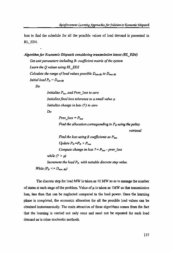
CRsinfMcement £earning flpproacfies for Sofution to 'Eamomk CDispatcn
loss to find the schedule for all the possible values of load demand is presented in
RL ED4.
Algorithm/or Economic Dispatch considering transmission losses (RL_ED4)
Get unil parameters including B- coefficient matrix of the system
Learn the Q values using RL_ED2
Calculate the range of load values possible Dmi/t (D) to Dwuu (D)
Initial load PD = Dmi1l (V)
Do
Inilialize Plos. and PreY _loss to zero
Initializejinalloss tolerance 10 a small value)l
Initialize change in loss (?) to zero
Do
PreY ~oss = P/oss
Find the allocation corresponding to PD using the policy
retrieval
Find the loss using B coefficients as Plc6s
Update PD =PD + Plou
Compute change in loss? = P10u - preY _loss
while (? > )l)
Increment the load PD with suitable discrete step value.
While (PD <= D1ftIU (V}
The discrete step for load MW is taken as 10 MW so as to manage the number
of states at each stage of the problem. Value of J.1 is taken as IMW so that transmission
loss, less than that can be neglected compared to the load power. Once the learning
phase is completed, the economic allocation for all the possible load values can be
obtained instantaneously. The main attraction of these algorithms comes from the fact
that the learning is carried out only once and need not be repeated for each load
demand as in other stochastic methods.
137

Chapter 5
The learning algorithms discussed in the previous sections have one limitation.
The input to each stage k of the multi stage problem is the amount of power to be
dispatched among remaining N - k units. This input power is discretized in order to get
defInite number of states at each stage of the problem. If the discretization step is
chosen to be a larger value, accuracy of the result will suffer while a smaller value
needs longer computation time. In order to make the algorithm more efficient
accounting the continuous value of input at each stage, a function approximation
strategy is proposed in the next section
5.10 Neural Network based solution using Reinforcement
Learning
The previous algorithms using Reinforcement Learning is based on fmding a
policy or mapping from fmite set of states to fmite set of actions. Learning is carried
out as a multistage process, taking an action from the _available action set when the
learning system is in any of the possible states in the state space. Initially, the state of
the system is represented by a tuple (0, PrJ, PD being the power to be allocated among
the N generating units. The learning proceeds by allocating certain amount of power to
one of the units and proceeding to successive stages until all the units are allocated. At
each step of learning. Q value corresponding to state -action pair is modifIed according
to the reward (cost of generation) of the action. Finally the Q values approach to
optimum and using the look up table of Q values, the optimum policy is retrieved as a
mapping of generating unit to power allocation corresponding to an input load value.
One limitation of this algorithm is that the state and action spaces are
discretised with certain value of step size. This may give some inaccurate result when
the discretization step is to be made large in the case of larger ranges of demand
values. Therefore one issue to be resolved is to somehow incorporate continuous nature
for the power input values at each of the stages in the multi stage solution process so
that solution is more efficient. One method that can be introduced is to use some form
138

'R,#nforcemmt £earnino jlpproacfies f(Jf So/UtWn to 'Economic (])ispatcft
of function approximation strategy in the learning process. In the next sections the
method of solution using function approximation strategy is presented.
S.10.1 Q learning through Function Approximation
When a continuous state space is considered, the state variable can take any
value in the continuous state space. Function approximation provides with a strategy in
which quantization of state space is not necessary. When Q learning technique is used,
Q values with respect to continuous state space are to be stored somehow. One
important fact is, in such cases Q values cannot be stored in a look up table. since the
values of state variable being of continuous nature. One solution is to construct a
function which will approximate the Q values at different cases based on some
parameters. That is, continuous state is denoted as x and represent Q values using a
parameterized class of functions Q(x, a, 0), where () is the parameter vector. With the
parameterized function to approximate Q value. Q - learning or learning optimum Q
values is to learn the optimum paramerer vector 0* so that Q (x. a. 9*) is a good
approximation of Q*Cx. a), V' x € Z , and V'a €c//. (Sutton and Barto [1998J. Imthias et
al. [2006]).
Therefore for making this learning through parameterized function possible,
first a suitable architecture or class of functions Q(x. a, 0) that is well suited for our
learning problem is to be decided. Secondly formulate a learning algorithm to get
optimum value of the parameter vector 0* which will give optimum Q
value, Q*Cx, a, 0).
In the literature, a variety of parameterized functions are found which can be
used for function approximation. Recently Neural Networks are being popularly used
for function approximation due to their extensive learning capability even with non
linear functions (Haykin [2002]).
Now, it is required to develop an algorithm to solve Economic Dispatch
problem using Reinforcement Learning and making use of a function approximating
network so that continuous nature of input variable can be accounted at each stage.
139

Cliapter 5
Then the algorithm will ultimately give a policy which is a mapping from the
continuous state space to discrete action space. For the same, as told earlier, the
Q values are represented using a parameterized class of functions Q (x, a, B) , where ()
is the parameter vector. The class of functions used is the Radial Basis Function
network, a category of Neural Network well suited for function approximation. The
outputs of this network represent the Q - values.
When Neural Networks are used, mostly supervised learning is employed to
train the network or adjust the weight vector elements. In such a case, a set of training
samples are needed which can be used to adjust the weight vector values. In the case
of Q learning, if supervised learning is employed one should be previously occupied
with a set of N training samples of the form,
{(x".a"):Q(x,,.a,,).k = 1, ......... ,N.x" Ez,a" EcA} in order to learn the
optimal weight values. Then the learning will turn to be a gradient descent method
such that {Q(x", a,,) - Q·(x", a,,)} is minimized. But in this case, such method is
impractical. since the exact values for Q. (x", a,,) is not known for any (Xk' a,,) pair.
Thus supervised mode of learning cannot be used to get the optimal weight vector of
RBF network which is going to be used as a function approximating network in the
Q learning method. A set of values of the form{(xk, ak, Xk+1),g(Xk, ak,X"+1)}, where
X,t is the current state, a,t is the current action, X.l:+J is the succeeding state of applying
action at and g(x". ak, Xk+l) is the reward corresponding to the particular transition of
state, are available. Now this information or set of examples can be used in some way
to learn the neural network for optimum weight adjustment. For the same,
Reinforcement Learning is used effectively so that optimum value of the parameter
vector O· is obtained resulting in optimum Q values. For exploring the action space,
just like in the previous algorithm e - greedy method is employed for action selection.
In our problem of Economic Dispatch, demand at each stage can be considered
as continuous. That is input power Dj to each of the stage is a continuous quantity and
the action at each stage (allocation to one particular unit) at is discrete. The objective is
to get a policy, which is a mapping from the continuous demand space to discrete
140

rJ(pnforcement Learning ){pproacfies for Solution to r&orwmic <Dispatcli
power allocation space. Learning optimal Q values involve learning the optimal
parameter vector (r such that QeD, a, 8*) is a good approximation ofQ*CD, a). Radial
Basis Function (RBF) neural network is used to store the same.
5.10.2 Architecture ofRBF Network
In this section, a novel architecture of the RBF network is proposed to store the
Q - values in the context of Economic Dispatch. Q - values of each stage is stored in
one RBF network. Thus for an N unit power system (N stage decision making
problem), there are N RBF networks. RBF network of all stages consist of an input
layer, hidden layer and an output layer. The input layer is made up of a single node for
connecting the input variable to the network. The hidden layer consists of 71Jj hidden
nodes. This layer applies a non linear transformation from the input space to the m
dimensional hidden space, 9lm• The output layer consists of nl linear nodes which
combine the outputs of hidden nodes (Hay1dn [2002J).
The architecture of the RBF network for the first stage is given in Fig 5.3
Fig 5.3 RBF network for Stage 1.
141

Cfiapter 5
The input to this RBF network is D}, the total power to be supplied by
generators G/t G}, ......... GN and output of the RBF network after learning is
Q·(Dl'aD,Q·(Dl'aD, ................ Q·(DlJa~l), where al, a~, ......... a~l are the
different actions possible at stage 1.
Similarly, the input to the RBF network of I(It stage is the power to be allocated
to generators Gb Gt+/t ...................... ,.GN, which is denoted as the state of the system
DIc.A1so,
The output of this network is Q(D",aD,Q(Dk,a~), ............ , Q(D",a;")
where nk is the number of actions or power allocations possible at J(" stage. The l"
output of the RBF network at 1(" stage is given by the expression:
(5.12)
where WQ" is nlX ml matrix ofreals, and WQk [i][l], •...... , WQt[i][m,,] are the
weights of the l" output unit; and { ~ j: fJ{' -> fJI, j = ], ........ mJ is a set of mic radial
basis functions which constitute the mic hidden units at j(" stage.
One can use the Gaussian function as the RBF. Then the output of l" RBF (ie,
l" hidden unit) at J(" stage is given by,
(5.13)
where c1 is the centre off' RBF at J(" stage and 0'1 is the width of the RBF at
l(" stage.
Substituting ~J (D,,) from equation (5.13) to equation (5.12) we get,
j=m"
Q(D",akJ 0) = Yk = I WQk [i]U]exp ((Dk - c1 )2)/2C1~) J=l
(5.14)
142

~inf()(cement Learning )fpproacfie.s for Solution to ~",lWmic CDispatcfi
where i ;:::: 1, .... nJ;. The RBF network at J(Ir stage described above is thus completely
specified by the parameter vector
where
Thus. finding a good approximation of the Q value using the RBF network
involves finding the optimum parameter vector 8· = [e·, u*, W·].
5.10.3 Learning Algorithm for Economic Dispatch (RL_ED5)
From the previous section it is concluded that finding the optimum parameter
vector, 8* = [c·,u·, W*] is the task to be resolved in finding the good approximation
of the Q value function. Next is, how to find the optimal parameters c·, u* and W*.
In the RBF network described above, adjusting the weights associated with a
given basis function, say /t basis function at It' stage • will affect the value of the
output only in a small region around the centre of /Ir RBF. c~. (For a value of input
DJ: Ef)l, away from c~, exp «Die - cbz /2uf) will be almost zero. This feature of
RBF network structure which indicates that each hidden layer neuron can be viewed as
approximating the target function over a small region around its centre makes it
possible to place the centres on a uniform grid spacing in order to get a better
interpolation of the input.
In the case of Economic Dispatch problem, first fix the number of hidden units
based on the generation limit constraints. The input to this It' RBF network is the
fraction of the power demand DJ: yet to be distributed among the remaining N - k
units. Therefore, number of hidden units in each RBF network basically depends upon
143

Chapter 5
the maximum and minimum possible demand at that particular stage. Le., for It" stage,
it depends on the values of Dmin(lc) and Dmaz(lc)o
For the first stage or first RBF network, the input will be equal to the power
demand PI>- i.e., DJ = PD-
Minimum and maximum ranges of power demand possible are calculated as
discussed previously. The number ofunifonnly distributed centres (hidden nodes) mJ at
this stage is decided by the range of Dmin(J) to D 1ftfU(J)' Similarly for It" stage, the number
of hidden nodes is decided by Dmill(k) and DIlfIJ%(k).
Once the number of hidden nodes is fixed, fmd the distance between centres of
Gaussian functions as,
gJ; = ( D1fI4%(k) - DmmruJ / (mk-J)
mk - Number ofRBF centres at It" stage.
Then the optimal values for the mk centres of the It" RBF network (eiJ are
chosen uniformly distributed between D mi1l(k) and DINU(k) as
( D",i1I(l). D",IIl(k) + gk, .............................. ..... Dmax(k)}
Next is to find the optimum values for the width of the RBF networks at the
different stages. Since the centres of the Gaussian functions form a uniform grid, width
of the Gaussian function (0) is taken as a suitable multiple of the distance between the
centres. This multiplication factor decides the percentage overlapping between the
successive functions. Thus width of the Gaussian distribution functions is calculated
as:
CT = spread factor + distance between centres, where spread factor is the
multiplication factor chosen to provide sufficient overlapping between successive
Gaussian functions. The spread factor can be chosen in the range 0.5 - 1 based on the
complexity of the problem.
Since the values for e; and ut are fixed, the task of learning now reduced to
fmding the optimum value for the third element in the optimum parameterised vector
(r or WQk• In other words, problem reduces to learning the Neural Network for the
optimum values ofthe weight matrix WQt [i]Ul, i = 1, ..... , nk,j = 1, .......... , mk'
144

CRJinforcement £eami1l{J .Jlpproacfies for SofutiQn to !Ecorwmic <Dispatcli
As mentioned earlier one can use of Q - learning strategy for getting the
optimum values for the parameter WQ". The network has to learn for the optimal values of the weight elements
WQ" [i] U] such that y/ would be a good approximation of Q" (Dk , ai). If the Q" values
are known for each stage corresponding to a large number of state action pairs, the
learning of the network is an easier task since one can go for supervised learning of the
weight matrix WQ". But the Q values in the initial stage are unknown and therefore
one cannot proceed in this direction. Q learning strategy is made use of to make the
network learn for the optimum values of weight matrix.
In the standard Q learning method, updating of Q value at each iteration 'n' is
given by the equation:
Qn+1 (Xk ,ale) = Qn (Xk • ak) + a[ (g(Xk • ale. Xk+l) + .., minaJEoilk+l Qn+1 (xk +1 ,at) - Qn (Xk, ak)]
(S.lS)
In the problem of Economic Dispatch, the next state or input to the next stage
is easily found out as,
Dk+1. = Dle• - a~ • where a~ is the power allocation denoted by the action
performed at It stage. That is, on selecting an action a~ from the action space ~.
input to the next RBF network is modified as the remaining power yet to be allocated.
In this context, for learning the weight vector elements, Q learning method is
formulated for modification of the weights. In the network, if the current state is D1c
and the action is a~. the updating has to be localized to the output node,
yk = Q(Dk• a~) or in other words the weight values connected to y/c need
only be modified while keeping the remaining weight values unchanged.
Since y~ ::0 L~:~kWQ" [i][j] 0j(Dk), to change yL WQt[i]U]. j = 1, .........• mk need to be modified. Therefore updating equations for Economic
Dispatch problem for each of the N-l stages are summarised as,
145

Cliapter 5
j == 1, ...... .... ,mk
(5.16)
j == 1, .......... , mle and l == 1, ....... , nk, l *' i
£1W~ [i] U] is given by the Q learning algorithm as:
A WQ~(i][ j] = a ( g(Dk, ale, Dk+1) + Y mina'E.Ak+1 Q~+l (Dk+1. a')
- Qn (~ , ale) ) 0 J (Dk )
(5.17)
The reward, g(Dk' ale, Dk+l) is the cost of generation of power corresponding
to action at. For the last stage (le = N - J) since there is no choice of action but to
allocate the power DN-J itself, i.e, action aN-J = DN-J. Therefore update equation is
expressed as:
where,
(5.18)
The weight values are updated iteratively during the learning phase. At the end
of learning. Q values will be approaching to optimum. The selection of Gaussian
distribution function as the functions defIning the hidden nodes, ma1ce the updating a
localized task which in turn improves the computational efficiency.
Once the learning is completed and the weight vector elements are converged,
the allocation schedule is obtained by just retrieving the action element at each stage
which corresponds to minimum Q values (greedy action). Thus the entire algorithm for
fmding the optimum allocation schedule is having two phases as in previous cases:
learning phase and policy retrieval phase. Learning phase is given as RL _ EDS.
146

'R,tinfMcement Learni1t£J flpproaclies for Sofutwn to P.ccnwmic a>ispatcn
Function Approximation algorithm/or Economic Dispatch (RL_ED5)
Read the parameters of the RL algorithm
Read the Generating unit details
Read the demanded load power to be dispatched PD
Fix suitable number of hidden nodes for each RBF network
Initialize input to the first RBF network DJ = PD
For each of the N stages
Do
End do
Find the different centres of the RBF network
Find the set of actions at each stage
( number of output nodes for each network)
Initialize all the weight vector elements as zero
For iteration =1 to TnaX_iteration
Begin
For k =0 to N-2
Do
Select an action a/from the action set .Ak using e - greedy strategy
End.
and check the feasibility of action
For a feasible action a;, Find the cost of generation Cost (aiD
Update the weight vector elements using eqn. (5.16)
Update the input parameter Dk+1 = Dj; - a;
Enddo
Find the cost of generation Cost (aN.J
Update the weight vector elements connected to YN-/
using eqn. (5.18)
147

Cliapter 5
Once the learning is completed, the allocation schedule corresponding to any
load value can be found by the policy retrieval phase as explained before, by fInding
the greedy action at each stage.
5.11 Performance of the Algorithms
The proposed Economic Dispatch algorithms are assessed using different
standard test cases. RL based Economic Dispatch can be applied for finding the
schedule for generating units when the cost of generation is provided in any of the
different forms like variable cost table, cost coefficient, non convex cost functions and
actual cost data from a plant. This becomes useful when the cost of power varies in
every block of time since the availability of power is practically a dynamic one.
Algorithms are coded in C language and compiled and executed in GNU
Linux environment. Performance evaluation is done with Pentium IV, 2.9 GHz, 512
MB RAM personal computer.
In order to validate the proposed algorithms and make a comparison among
them, fIrst a three generator system with cost data given in a tabular form is considered
(Wood and Wollenberg [2002]). The first three algorithms are executed to find the
dispatch and a comparison of execution time is made.
Then IEEE 30 bus system with six generating units is taken in order to prove
the efficacy of the proposed approaches. The suitability of the proposed algorithms for
a system having generating units with piecewise cost functions is studied by
considering a 10 generator system In the case of Reinforcement Learning algorithms,
there is no need of getting exact cost functions. It is evident from the execution results
for the stochastic cost details.
The last two algorithms are validated and compared with the other recent
methods like simulated annealing and partition approach algorithm by considering a
standard test case, IEEE 6 bus system with three generators. The flexibility of the
proposed approach is investigated for system with 20 generating unit having given cost
functions.
148

'R.!inforcement Learnina Approaclies for Solution ro P.conomic (J)ispatcfi
In order to apply Reinforcement Learning algorithms, first the learning
parameters are to be ftxed based on the problem environment. The learning parameter &
accounts for rate of exploration and exploitation needed. Since it indicates a
probability, it can take any positive value less than 1. A small ftxed value may result in
premature convergence of the learning algorithm while a large ftxed value may make
the system oscillatory. Therefore in these RL based algorithms, a value of 0.5 is
assumed initially providing sufficient exploration of the search space and is decreased
by a small factor successively.
Discount parameter y accounts for the discount to be made in the present state
for accounting of future reinforcements and since in the case of Economic Dispatch
problem, the cost of future stages has the same implication as the cost of the current
stage, value of'1 is taken as 1.
The step size of learning is given by the parameter CL and it affects the mte of
modiftcation of the estimate of Q--value at each iteration step. By trial and error CL is
taken as 0.1 for achieving sufficiently good convergence of the learning system. The
RL pammeters used in the dispatch problem are also tabulated in Table 5.1
Table 5.1- RL Parameters
& 0.5
a 0.1
r 1
Case I - Three Generator system
First a simple example with three generating units (Wood and Wollenberg
[2002]) is considered for validating and explaining the RL approach of solution. The
transmission losses are neglected in this case. The cost details are given in tabular
149

Cnapter 5
form, which can be obtained from experience in case of a practical system. The unit
characteristics are given in Table 5.2, where Cl stands for the cost of generating P MW
by {"unit.
Table5.2 - Cost Table for three generator system
P(MW) Cl C2 C3
0 100000 100000 100000
25 100000 100000 100000
50 810 750 806
75 1355 1155 1108.5
100 1460 1360 1411
125 1772.5 1655 11704.5
150 2085 1950 1998
175 2427.5 100000 2358
200 2760 100000 100000
225 100000 100000 100000
The three generating units are having the minimum and maximum power
. generation possible as (50,200), (50,150) and (50,175). The discretization step for state
space and action space, S. and S. are taken as 25 MW for simplicity and fast
computation.
Therefore, Dmin(O) = 150 Dmax(O) = 525
Dmin(J) = 100 Dmax(J) =325
and Dmin(1) = 50 Dmax(1) =175
The Learning Automata solution (RL_ED1) was run for a demand of300 MW.
After 1000 iterations the learning process converged (performance index values remain
150

1?firiforcement Leami1l{J )'Lpproaclies for Sofuticn to P,conomic CVispatcli
unchanged). At this point the minimum value of performance index (Qak) is found out
as Rs. 4168 1- and the corresponding action ak corresponds to the optimum allocation
schedule.
In order to understand the perfonnance of RL algorithms (RL_ED2 and
RL_ED3), the different components of the multi stage decision process are to be
identified. The state tuples is of the form (k, DJ. Dk being the power to be dispatched
at JIlt stage.
Then, State space Z = Zo U Xl U X2 where
Xo = { (0,150), (0,175), (0,200), .............. (0,525)}
Xl = { (1,100), (0,125), (0,150), .............. (O,325)}
and X2
= {(2,50), (2,75), (2,100), .............. (0,175)}
Now identify the action space, which is a dynamic one since it depends on the
value of power Dk to be dispatched. The minimum and maximum values of actions are
found out as
Mino = (Do -D",ta(J) or P mJ,,(O) whichever is greater
Maxo = (Do - D",in(J) or P 1/fIJX(Q) whichever is smaller
Max] = (DJ - D"'iIt(J) or P 1/fIJX(J) whichever is smaller
For the purpose of explaining the algorithm, let the random value generated for the
demand is 300 MW. Then the action space at stageo is
cAo = {50, 75, .......... ,200}
One of these actions is selected and it passes to the next stage k =1. Then the
action space cAl is identified and action selection continued which brings out the
remaining power as the allocation for the last machine. Each time cost corresponding
to the power allotted is found out using the cost table given and Q value of the
151

Cliapter 5
corresponding state action pair is updated. Allocation to each unit is then found out as
the action which gives the minimum Q value corresponding to state comprising the
particular stage number (unit) and the power to be allotted. That is, argmina(Q(xk> a)
gives the allocation for K" unit for the power demanded D". Similarly the action
(allocation) corresponding to each of the units (1 = 0 to N-J) is found, calculating DJ: at
each stage of allocation.
The three algorithms RL_EDl, RL_ED2 and RL_ED3 are executed. The
allocation schedule obtained is obtained as (50,100,150) and the cost of generation is
Rs. 4168/-. The execution time for both the learning and retrieval algorithms is 2.034,
2.567sec. and 1.754sec. respectively. Once the learning is completed, using policy
retrieval phase, power schedule for any value of possible input demand values can be
retrieved.
The three algorithms are run for various the values of power demand
D",III(O)<=PD <=Dmtu(O) ie. 150<=PD<=525. !>art of the simulation result is tabulated in
Table 5.3 which is consistent with results given in (Wood and Wollenberg [2002]).
Table S.J - Allocation schedule for three generator system
D(MW) Pl(MW) P2(MW) P3(MW) Cost(Rs.)
250 50 50 150 3558
275 50 150 75 3868.5
300 50 100 150 4168
325 50 125 150 4463
350 50 150 150 4758
375 100 125 150 5113
400 100 150 150 5408
425 125 150 150 5720.5
450 150 150 150 6033
475 175 150 150 6375.5
500 200 150 150 6708
152

tRsinforcemtnt £lamina Approad!es for So(ution to 'Economic ,Visptztcn
For comparing the efficacy of the two algorithms, Simulation time for the three
algorithms are compared in Table 5.4
Table 5.4 Comparison execution time (or RL_EDI, RL_E02a.d RtEDJ
RL EDI RL_ED2 RL EDJ
No: of iterations 10000 100000 50000
Computation
time(sec.) 2.034 2.567 1.754
A graphical layout of the comparison is given in fig 5.4.
3
2.567 sec
2.5
2 2.034
• Rl_EDl
• Rl_ ED2
• Rl_ ED3
o +----~-
Fig 5.4 Comparison of execution time of RL approaches
On comparing the computation time of the algorithms, Learning Automata
method gives lesser time compared to {; -greedy solution. {; -greedy provides a simple
solution method compared to pursuit method. Pursuit strategy is faster compared to
other two methods. Since execution time is less. all the three algorithms seem to be
153

Cliapter 5
suitable for such smaller systems. But on analyzing the algorithmic steps, it is found
that for larger systems, Learning Automata is not preferable due to the large action
space to be handled which increases the memory requirement. The other two
algorithms are suitable for larger systems due to the multi stage formulation in the
solution procedure.
Case H -IEEE 30 bu system
To prove the flexibility for larger systems and to make comparison, the
proposed algorithms are now tested for IEEE 30 bus system consisting of six
generators (Somasundaram and Kuppusamy [2005]), without considering the
transmission losses. 1be system cost data is given in quadratic cost coefficient form as
given in Table 5.5. ie, for any power P, cost of generation is given out by the equation
C(P) = Ca + Cb·P +Cc·p2 , where Ca, Cb and Cc are the cost coefficients.
Also the maximum and minimum generations possible for each of the 6 generators are
specified.
Table 5.S - Cost coefficients for IEEE 30 bus system
Ca Cb Cc Pmin(MW) Pmax(MW)
561 7.92 0.001562 150 600
310 7.85 0.00194 100 400
78 7.978 0.00482 50 200
102 5.27 0.00269 100 500
51 9.9 0.00172 40 350
178 8.26 0.00963 100 280
The maximum generation possible with these 6 generators turns out to be 2330
MW while minimum generation is 540 MW. Since the number of action vectors
increases to a very large value Learning Automata method is not preferable when the
number of generators is increased The RL algorithms (Rl_ ED 1, RL _ ED2, RL _ ED3
and RL _ ED5) are now applied to get the economic allocation for the six units.
154

£%inforcement £eamiTl{} )fpproacfies for Sofution to P.conomic ([)ispatcn
The discretization step for action and state space are taken as 10 MW as
balance between the accuracy and size of the state and action spaces. At each step of
iteration, action is selected according to the exploration method. The Q values of state
action pairs are updated for which cost of generation is calculated by evaluating the
quadratic equation.
Even after two hours of execution, optimum schedule is not obtained for
RL_ED1. This is because of the large number of combinations available in the action
space.
In RL_ED2, after 5x1Os iterations the Q values approach optimum while
RL_ED3 converged in 2x10⁵ iterations. The optimum dispatch is found out by tracing
out the greedy action which give out minimum Q value corresponding to a particular
state Dk as k vary from ° to N-l. The optimum schedule for the different values of
power demand is obtained using the policy retrieval phase. Schedule for the entire load
values ranging from 540 MW to 2330 MW is obtained. The entire schedule is obtained
in 23.87sec. using RL_ED2 and in 15.63 sec. with RL_ED3 which proves the
suitability of the algorithms
In order to apply Neural Network approach for solution, first the number of
centres in the RBF network and the spread factor of the Gaussian distnbution function
are to be decided. The number of centres decide the number of interconnections and
hence the size of the weight matrix. In Economic Dispatch problem, the number of
centres is decided by the range of demand input to each stage of the multi stage
decision task. Demand range in the last stages is much smaller compared to the initial
stages. Therefore for increasing the computational efficiency, more number of centres
is selected at the initial stages compared to later ones. Here the number of centres is
taken as 30, 30, 20, 20, 16 and 16. By trial and error spread factor of 0.7 is selected.
The solution procedure RL_ED5 is executed for learning the network. The six RBF
networks are made to adjust the weights and the learning converged in 5 x 10 6
iterations with 14.89sec.
155

Cliapur 5
The number of iterations required is more in the function approximation
method. But since the number of weight values to be adjusted is less than the number
of Q values, execution time is decreased.
The algorithms are executed in several trials and the cost and allocation
schedule obtained are almost the same with negligible error in the different trials and
with RL_ED2, RL_ED3 and RL_ED5.
A part of the allocation schedule corresponding to various values of power
demand in steps of 100MW is tabulated in Table 5.6.
Table 5.6 - Allocation schedule for IEEE 30 bus system
D(MW) P1(MW) P2(MW) P3(MW) P4(MW) P~(MW) P6(MW) Cost(Rs.)
600 150 100 50 160 40 100 5951.611
700 150 100 50 260 40 100 6591.591
800 150 100 50 360 40 100 7285.371
900 150 100 50 460 40 100 8032.951
1000 160 150 50 500 40 100 8847.839
1100 210 190 60 500 40 100 9698.202
1200 260 220 80 500 40 100 10563.33
1300 310 260 90 500 40 100 11443.07
1400 350 300 110 500 40 100 12337.4
1500 400 340 120 500 40 100 13246.5
1600 440 380 140 500 40 100 14170.28
1700 500 400 160 500 40 100 15109.32
1800 580 400 180 500 40 100 16070.22
1900 600 400 200 500 100 100 17070.12
2000 600 400 200 500 180 120 18108.22
2100 600 400 200 500 270 130 19175.55
2200 600 400 200 500 350 150 20272
2300 600 400 200 500 350 250 21483.2
156
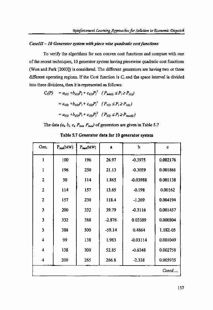
IR/inforcement Learning ;fpproacfzes for So(ution to 'Ecurwmic tDispatcli
CaseIll-10 Generator system with piece wise quadratic cost functions
To verify the algorithms for non convex cost functions and compare with one
of the recent techniques, 10 generator system having piecewise quadratic cost functions
(Won and Park [2003]) is considered. The different generators are having two or three
different operating regions. If the Cost function is Cl and the space interval is divided
into three divisions, then it is represented as follows:
Ci(P} = al(!) +bl(IJ'; + CI(JJ'/ (P ",i1I(i) ~ Pi ~ Pi(l;)
= ai(2) +bl(1J'1 + Ci(1J'/ (Pi(!) ~ PI ~ P j (1)}
= aim +b;(3J'1 + CI(3J'/ (Pi(2) ~P,~ P",ax(i)}
The data (a;. bu Cu P",w P ~ of generators are given in Table 5.7
Table 5.7 Generator data for 10 generator system
Gen. Pmia(MW) PIIIU.(MW) a b
1 100 196 26.97 -0.3975
1 196 250 21.13 -0.3059
2 50 114 1.865 -0.03988
2 114 157 13.65 -0.198
2 157 230 118.4 -1.269
3 200 332 39.79 -0.3116
3 332 388 -2.876 0.03389
3 388 500 -59.14 0.4864
4 99 138 1.983 -0.03114
4 138 200 52.85 -0.6348
4 200 265 266.8 -2.338
c
0.002176
0.001861
0.001138
0.00162
0.004194
0.001457
0.000804
1. 18E-05
0.001049
0.002758
0.005935
Contd ....
157

Cfiapter 5
Table 5.7 Contd ...
5 190 338 13.92 -0.08733 0.001066
5 338 407 99.76 -0.5206 0.001597
5 407 490 53.99 0.4462 0.00015
6 85 138 1.983 .{).03114 0.001049
6 138 200 52.85 -0.6348 0.002758
6 200 265 266.8 -2.338 0.005935
7 200 331 18.93 .{).1325 0.001107
7 331 391 43.77 -0.2267 0.001165
7 391 500 43.35 0.3559 0.000245
8 99 138 1.983 .{).03114 0.001049
8 138 200 52.85 .{).6348 0.002758
8 200 265 266.8 -2.338 0.005935
9 130 213 14.23 .{).01817 0.000612
9 213 370 88.53 .{).5675 0.001554
10 362 407 46.71 '{).2024 0.001137
10 407 490 61.13 0.5084 4.16E'{)5
10 407 490 61.13 0.5084 4. 16E'{)5
The system is made to learn using the algorithms given in RL_ED2, RL_ED3
and RL_ED5 and the Q values approach optimum in 107, 5 X 10⁶ and 1.5 x 10⁷
iterations respectively. The same values of learning parameters are taken as in previous
cases. The discretization step for state and action spaces is taken as IOMW.
158

CRsinforcement £eamins }fPJ1fOacfUs for So{utjqn to P.corwmic <Dispatcli
Allocation schedule corresponding to values of power demand ranging from
1400 MW to 3000 MW obtained are given in Table 5.8. The times of execution are
42.87sec., 38.69 sec. and 34.95 sec. respectively. The cost and allocation schedule
obtained are comparable with that of improved genetic algorithm (Won and Park
[2003]).
Table 5.8 - Part of Schedule - 10 generator system
Demand
(MW) PI P2 P3 P4 Ps P6 P7 p. Pg PlO Cost(Rs.)
1400 100 170 200 190 190 150 50 200 50 100 903.30
1500 100 190 200 210 210 150 90 200 50 100 948.3638
1600 100 200 200 220 230 150 150 200 50 100 996.4249
1700 100 210 200 240 240 150 210 200 50 100 1047.349
1800 100 220 200 260 270 ISO 250 200 50 100 1101.472
1900 100 220 200 310 320 150 250 200 50 100 1164.422
2000 100 220 200 360 370 150 250 200 50 100 1237.691
2100 110 220 200 400 420 150 250 200 50 100 1321.016
2200 120 220 210 430 450 150 250 220 50 100 1411.387
2300 140 220 230 450 470 ISO 250 240 50 100 1507.16
2400 ISO 220 250 480 490 150 250 260 50 100 1608.295
2500 170 220 280 500 500 150 250 280 50 100 1715.796
2600 190 220 310 500 500 150 250 320 50 110 1833.078
2700 210 220 350 500 500 150 250 350 50 120 1960.531
2800 230 220 380 500 500 150 250 380 60 130 2097.839
2900 250 220 410 500 500 160 250 400 70 140 2244.236
3000 250 220 440 500 500 170 250 440 80 150 2399.784
159

Cliapter 5
Case IV ( IEEE 6 bus system Considering Transmission losses)
Next is to validate the solution approaches taking into account the transmission
network losses occurring in the system. For testing the efficacy of solutions RL_ED4
and RL_ED5, considering the transmission losses, a three generating unit system with
given loss coefficients is considered. While executing RL _ ED5 the same procedure of
updating of demand is carried out with the schedule obtained at each time from the
Neural Network. Standard IEEE 6 bus system which is having three generating units
and eight lines (Lin and Gow [2007]) is taken for case study. The fuel cost curve of the
units is represented by a third order polynomial function:
C,(Pt) = at + btPt + ctpl + dtP?
The associated fuel cost coefficients and B-matrix. parameters are given in
Table 5.9.
Table 5.9 Generator data and Loss Coefficients of IEEE 6 bus system
Generator data
Unit No 1 2 3
ai 11.1 -631 147.144
bi 5.101 13.01 4.18997
Cl -1. 64E-03 -3.06E-Ol 3.08E-04
dl 3.33E-06 3.33E-05 -I. 77E-07
P",bJ(MW) 100 100 100
P 1ItIJX(MW} 500 500 1000
B Coefficients
1 7.50E-05 5.00E-06 7.50E-06
2 5.00E-06 1.50£-05 1.00£-05
3 7.50E-06 1.00E-05 4.50£-05
160

rJ?!inforcement Learning .:APF'oacMs for Sowtion to I£.conomic ([)ispatcli
The learning is first carried out using RL_ED2. Then RL_ED4 is executed to
fmd out the dispatch for all the possible load values ranging from 500MW to
1900MW. For getting accurate schedule, the discretization step taken is 2MW. The
remaining power of the demanded value « 2MW), which is negligibly small compared
to the total demand is randomly assigned to one of the units without exceeding
maximum limit. Number of iterations required is 9 x 10" and the time of execution is
14.87 sec for getting schedule for all the load values.
In order to apply the function approximation strategy using Radial Basis
function networks (RL _ E05), Number of RBF centers is taken as 80, 60 and 40 and
the action step is taken as low as 2MW for accounting the losses more effectively.
RL_ED5 is executed to learn the Q values. The schedule is obtained for all the load
values in suitable steps. The learning algorithm converged in 2 x lOs iterations and the
total time taken is only 12.98 sec.
The obtained schedule and costs are tabulated in Table 5.10.
Table 5.10 Schedule and cost obtaIned for IEEE 6 bus system
Po(MW) Pg1(MW) Pg2(MW) Pg)(MW) Cost Loss(MW)
500 100 100 306 2383 6
600 100 100 409 2800 9
700 261 100 373 3246 14
800 298 100 420 3696 18
900 330 100 495 4140 25
1000 338 100 591 4737 29
1100 341 100 691 5200 32
1200 344 100 800 5679 44
Contd ...
161

Cnapter 5
Table 5.10 Contd ....
l300 414 100 835 6002 49
1400 446 156 851 6474 53
1500 453 229 874 6896 56
1600 461 300 899 7438 59
1700 469 302 992 7772 64
1800 455 321 991 8320 67
1900 487 492 996 8801 75
Case V - IEEE 30 bus system with transmission system parameters
In the previous case, the transmission network loss is represented through B
coefficients. For validating the algorithm while considering the entire transmission
system representation, consider IEEE 30 bus system with entire transmission system
parameters. The transmission line parameters are given in Table 5.11.
Table S.11 Line data-IEEE 3();'bu5 system
Branch
no. From To R(pu) X(pu) Y/2 (pu)
1 2 I 0.0192 0.0575 0.0264
2 1 3 0.0452 0.1852 0.0204
3 2 4 0.057 0.1737 0.0184
4 3 4 0.0132 0.0379 0.0042
5 2 5 0.0472 0.1983 0.0209
6 2 6 0.0581 0.1763 0.0187
7 4 6 0.0119 0.0414 0.0045
Contd ...
162

tR/inforcement Learnino ;4pproaclies far SolUtion ro P.comnnic (])ispatcfi
Table 5.11 Contd ...
8 5 7 0.046 0.116 0.0102
9 6 7 0.0267 0.082 0.0085
10 6 8 0.012 0.042 0.0045
13 9 11 0 0.208 0
14 9 10 0 0.11 0
16 12 13 0 0.14 0
17 12 14 0.1231 0.2559 0
18 12 15 0.0662 0.1304 0
19 12 16 0.0945 0.1987 0
20 14 15 0.221 0.1997 0
21 16 17 0.0824 0.1932 0
22 15 18 0.107 0.2185 0
23 18 19 0.0639 0.1292 0
24 19 20 0.034 0.068 0
25 10 20 0.036 0.209 0
26 10 17 0.0324 0.0845 0
27 10 21 0.0348 0.0749 0
28 10 22 0.0727 0.1499 0
29 21 22 0.0116 0.0236 0
30 15 23 0.1 0.202 0
31 22 24 0.115 0.179 0
32 23 24 0.132 0.27 0
33 24 25 0.1885 0.3292 0
34 25 26 0.2544 0.38 0
35 25 27 0.1093 0.2087 0
38 27 30 0.3202 0.6027 0
39 29 30 0.2399 0.4533 0
40 8 28 0.0636 0.2 0.0214
41 6 28 0.0169 0.0599 0.0065
163

Cliapter 5
The six generators are located at buses: 1, 2, 5, 8, 11 and 13, and the cost
coefficients are the same as given in Table 5.5. A total load of283 MW is connected to
the different buses as given in the Table 5.12.
Table 5.12 Load data-IEEE 30-bus system
Qo
Bus no. Po (MW) (MW)
1 0 0
2 21.7 12.7
3 2.4 1.2
4 7.6 1.6
5 94.2 19
6 0 0
7 22.8 10.9
9 0 0
10 5.8 2
11 0 0
12 11.2 7.5
14 6.2 1.6
15 8.2 2.5
16 3.5 1.8
17 9 5.8
18 3.2 0.9
Contd ...
164

1?[injorcement Leami11fJ jfpproacfies for So{ution to r£conomic CDispatcli
Table 5.12 Contd ...
19 3.2 1.6
20 2.2 0.7
21 17.5 11.2
22 0 0
23 3.2 1.6
24 8.7 6.7
25 0 0
26 3.5 2.3
27 0 0
28 0 0
29 2.4 0.9
30 10.6 1.9
In this case, transmission losses are calculated by executing fast decoupled
power flow solution. In this case since the connected load is given as 283MW, we fix
the initial demand as the 283MW. First, the learning algorithm takes the total demand
PD = 283 MW. After sufficient number of iterations, the Q values approach optimum.
Then by policy retrieval phase, an economic schedule is obtained. The power flow
algorithm is executed to get the transmission losses in the system. The loss MW is used
to update the initial demand to the solution algorithm and new schedule is obtained.
The updating is continued until the iterative algorithm is converged. giving tolerable
value of updating for the loss in two successive iterations. The results are given in
TableS.l3.
165

Cfiapter 5
Table 5.13 Economic Schedule for IEEE 6 bus system
Po(MW) Pg1(MW) Pg2(MW) Pg3(MW) Cost(Rs.) Loss(MW)
283 45 100 142 1576 4
Case VJ- Three unit system with stochastic data
One important point to be considered while formulating the algorithm for
Economic Dispatch is its flexibility for the different cost functions. In practical
situation cost of generation for the same MW power may not be the same constant
always. It exhibits randomness due to various factors. To prove that the proposed
algorithms efficiently handle the randomness in cost values, next consider the cost
given in terms of mean and variance. The cost values are given in Table 5.14 for a
three generating unit system. Cl indicates the cost of generating power P MW by l"
unit.
Table 5.14 Cost details with given variance of three generator system
P(MW) Cl C2 C3
Mean variance Mean variance Mean variance
0 100000 100000 100000
25 100000 100000 100000
SO 810 60 750 100 806 60
75 1355 80 1155 100 1108.5 80
100 1460 100 1360 80 1411 100
125 1772.5 100 1655 100 11704.5 100
150 2085 100 1950 80 1998 80
175 2427.5 80 100000 2358 80
200 2760 60 100000 100000
225 100000 100000 100000
166

~nforcement £earning Jlpproacnes for So(utilm to £Economic <Dispatcli
The three solution steps (RL_EDl, RL_ED2, RL_ED3 and RL_ED5) are
executed to get the schedule for all the possible load values in steps of 25 MW. In case
of RL_ED5, for simplicity the same number of RBF centers is taken in all the three
networks. 12 centers are taken for this case. Spread factor of 0.7 is chosen by trial and
error to get reduced computation time and sufficient accuracy for the result. The entire
schedule is obtained in 2.03 sec., 2.70 sec., 2.05sec. and 1.82 sec respectively. The
obtained allocation values are given in Table 5.15.
Table 5.15 Schedule obtained for stocbastic data
D(MW) Pl(MW) P2(MW) P3(MW) Cost(Rs.)
150 50 50 50 2353
175 50 50 75 2674
200 50 100 50 2989
225 50 100 75 3326
250 50 SO 150 3592
275 50 150 75 3902
300 50 100 150 4150
325 50 125 150 4466
350 50 150 150 4742
375 100 125 150 5109
400 100 150 150 5394
425 125 150 150 5735
450 150 150 150 6067
475 175 150 150 6431
500 200 150 150 6745
525 50 50 125 13241
167

Chapter 5
Case VII - 20 Generator system
For validating the efficacy of Reinforcement Learning based algorithms for
large systems, next a 20 generator system is considered. The cost function is given in
quadratic fonn. The unit details are given in Table 5.16.
Table 5.1fr Generator Details of 20 generator system
Unit c. Cb Cc Pmin(MW) Pmu(MW)
1 1000 18.19 0.00068 150 600
2 970 19.26 0.00071 50 200
3 600 19.8 0.0065 50 200
4 700 19.1 0.005 50 200
5 420 18.1 0.00738 50 160
6 360 19.26 0.00612 20 100
7 490 17.14 0.0079 25 125
8 660 18.92 0.00813 50 150
9 765 18.97 0.00522 50 200
10 770 18.92 0.00573 30 150
11 800 16.69 0.0048 100 300
12 970 16.76 0.0031 150 500
13 900 17.36 0.0085 40 160
14 700 18.7 0.00511 20 130
15 450 18.7 0.00398 25 185
16 370 14.26 0.0712 20 80
17 480 19.14 0.0089 30 85
18 680 18.92 0.00713 30 120
19 700 18.47 0.00622 40 120
20 850 19.79 0.00773 30 100
168

~forcement £eamino llpproaches for Sofutwn to P.cOMmic CDispatcli
The transmission loss is calculated using B coefficient matrix. Algorithm
RL_ED4 is executed to give the schedule for the range of load from 1000MW to
3OO0MW. The execution time taken is 45.87sec. Part of the schedule and the loss are
tabulated in Table 5.17.
Table 5.17 Schedule for 20 generator system
D(MW) 2000 2500 3000
PI 421 498 530
P2 140 159 167
P3 105 120 140
p .. 94 118 135
Ps 81 92 97
P6 51 74 87
P7 89 115 141
Ps 81 106 162
P9 84 103 155
PlO 70 98 108
PII 236 290 358
P12 89 120 136
P13 82 119 124
PI .. 90 115 147
PIS 23 30 70
PI7 64 87 111
PI9 72 100 106
P20 45 54 75
Loss 39 64 81
169

Cfiapter 5
5.12 Evaluation of Algorithms
The different Reinforcement Learning algorithms have been tested for their
efficacy and performance. The computation time of the different RL algorithms for the
different test cases are tabulated for comparison in Table 5.18.
Table 5.18 Comparison of Computation times of different RL algorithms
(rime in sec.)
RL ED1 RL_EDl RL_ED3 RL_ED4 RL_ED5
Three gen system with 2.034 2.567 1.754 1.465
given cost table,
neglecting
transmission loss
IEEE 30 bus system Not 23.87 15.63 14.89
with 6 generators, giving
neglecting optimum
transmission losses result
10 generator system 42.87 38.69 34.95
with piecewise
quadratic cost
coefficients
IEEE 6 bus system 9.87 6.98
with 3 generators,
considering
transmission losses
3 generator system 2.03 2.70 2.05 1.82
with stochastic cost
data
170

lRsinforcement Leamif1(J Approacfies for So{ution to c£conomic rDispatcli
In order to highlight the efficacy and computational speed of the developed
algorithms, the results of RL_ED4 and RL_ED5 are compared with other recently
developed algorithms.
For comparing with other recent techniques, IEEE 6 bus system (Case IV) with
a load power of l200MW is considered.. That is, the initial demand to the system is
l200MW and the corresponding schedule is obtained. The optimal cost is obtained as
Rs.5679.2 and the power loss calculated is 44MW. The time taken by our proposed
algorithm is only 9.87 sec and 6.98sec. for RL_ED4 and RL_EDS. The obtained
schedule is tabulated and a comparison is made with other stochastic techniques (Wong
et al.[1993] and Lin et al.[2007]) in Table 5.19. The dispatch schedule obtained is
comparable. Transmission loss in all the case is nearly 43MW.
For getting the schedule for 10 different load values RL_ED4 took only 10.56
sec, while RL_ED5 was executed in 7.l2sec. For other methods, the time needed is
nearly 10 times the time for single load value. This directly highlights the efficiency of
Reinforcement Learning approach for giving schedule for any forecasted load profile
instantaneously.
Table S.19 Comparison with SA and P AA
Method PAA SA RL ED4 RL EDS
Pg\(MW) 362.2 342.8 344 343
Pg2(MW) 100 100 100 100
Pg3(MW) 781.4 801.4 800 800
Cost(Rs.) 5671.06 5682.32 5679.2 5676
Loss(MW) 43.68 43.8 44 43
Time (sec) 16.82 27.253 9.87 6.98
171

Cli4pur 5
A graphical comparison is also given in Fig 5.5
30
25
20
15
10
5
o
. 5A
. PAA
• Rl_ED4
• Rl_ED5
Fig !S.S Comparison or execution time with other methods
The above comparison directly depicts the improved performance of
Reinforcement Learning based so lutions over other recent methods. This faster
scheduling provided by Reinforcement Learning in effect helps to improve the
economy of generation.
5.13 Conclusion
Even though many techniques are applied for the solution of Economic
Dispatch problem, Reinforcement Learning provides a good methodology due to its
faster computing speed and simplicity. Once the learning phase is completed, schedule
for any load demand can be obtained instantaneously. Also it can effectively handle
the stochastic cost functions associated with practica l thennal units. The developed
algorithms are applied on different test systems. In all these cases sat isfactory
perfonnance is obtained. The result when compared with other stochastic techniques is
found to be better. As a further step in this direction algorithm incorporating additional
constraints such as ramp rate limits, valve point effects etc. existing in power systems
can be developed.
172

CHAPTERS
REINFORCEMENT LEARNING
APPLIED TO AGC WITH
COMMON SYSTEM FREQUENCY
6.1 Introduction
Automatic Generation Control (AGC) constitutes the on line dispatch part of
generation control. Electrical energy is generated by the generators at the generating
stations, transformed into suitable voltage level by the transformers and dispatched
through various buses to the loads which consume the electric power. In an
interconnected system, the overall power system is divided into several grids or pools,
each comprising several subsystems. Through Tie lines the system is connected to the
neighbouring systems belonging to the same grid (POOl). The active power demand in
the system is met by the combined generation of all the generating sources in the
system. Considering the economic perspective of power generation, the forecasted load
demand is distributed among the generating units in the system in the most economic
manner by the pre dispatch control. It consists of Unit commitment and Economic
Dispatch at each control area.
Once the pre dispatch or pre scheduling is over, the generating units will be
entitled to generate the allotted power, (fraction of the forecasted load demand) for the
specified duration of time. Instantaneous addition and removal of load in the system
will be reflected by a change in the system frequency. Considerable drop in frequency
result in high magnetizing currents in induction motors and transformers and decline
their performance. Control of system frequency ensures constant speed for the
frequency dependent load such as induction and synchronous motors and thus their
efficient operation. Thus for satisfactory operation of a system, frequency should be
maintained constant. The frequency of the system is dependent on active power
173

Cfiapter6
balance. A change in active power demand at one point is reflected by a change in
frequency. Since there is more than one generator supplying power to the system the
demand is allocated to the different generators.
In case of interconnected system with two or more independently controlled
areas, in addition to the control of frequency, generation within each area is to be
controlled so as to maintain scheduled power interchange. When the entire
interconnected system is operating on a common system frequency, instantaneous load
variations in any of the control area will affect the common system frequency. This
makes the task more difficult to solve as the load is not predictable always. Also the
generation capacities and the means by which generation can be changed are limited.
Even though primary control action is served by the speed governor associated
with the generating units, supplementary control is needed to reallocate the generation
so as to bring the frequency to exact scheduled value. Supplementary control can be
done manually by setting the reference point so as to increase or decrease the
generation. Automatic functioning of this supervisory or supplementary control action
is referred to as Automatic Generation Control. Automatic Generation Control problem
is discussed in the next section.
Reinforcement Learning approach for solving the AGe problem for an
interconnected system (Imthias et al. [2002]) is extended in the next sections with an
approach of common system frequency.
6.2 Automatic Generation Control problem
In a large interconnected power system with several pools having many
number of generators, manual regulation is not feasible and therefore automatic
generation and voltage regulation is essential.
Once a generating unit is tripped or a block of load is added to the system, the
power mismatch is initially compensated by the extraction of kinetic energy from
system inertial storage which causes a decline in system frequency. As the frequency
decreases, power taken by loads decreases. Equilibrium for large systems is often
174

<R.Pnforcement £eamine Jlppfiea to Jlqc 'Witn Common System Prequency
obtained when the frequency sensitive reduction of loads balances the output power of
the tripped unit or that delivered to the added block of load at the resulting new
frequency. If this effect halts the frequency decline, happens in less than 2 seconds.
If the frequency mismatch due to the addition of load M\ is large enough to
cause the frequency to deviate beyond the governor dead band of the generating units
(generally in the range of 30-35mHz.), their output will be increased by the governor
action. For such mismatches, equilibrium is obtained when the reduction in the power
taken by the loads plus the increased generation due to governor action compensates
for the mismatch. Such equilibrium is often obtained within 10-12 seconds. Typical
speed droop are in the range of 5% and therefore at the expense of some frequency
deviation, generation adjustment is carried out by governors.
On attaining the new equilibrium state after variation in the load M\,
where #' is the change in frequency and D is the damping constant.
Lumped parameter model of the generation system is commonly used for the
analysis of AGe systems (Elgerd [1982]). In such representation, the aggregate
frequency sensitivity of all loads is represented by a damping constant. The
perturbation model of a lumped parameter system is given in Fig 6.1.
Fig 6.1 Perturbation model
175

Cliapter 6
In this model, M represents the aggregated inertia constant and D is the
damping constant. If there is no additional frequency control, the change in the
mechanical power output Pm is zero. Hence, the system response to load change Lll'L is
determined by the inertia constant and damping constant.
Each generating unit is equipped with a speed governor mechanism, which
provides the function of primary frequency controL But for compensating the offset
deviation and bringing back to the original scheduled frequency, a manual or automatic
(through AGC) follow up and corresponding control are required.
Fig 6.2 represents the equivalent model including the governor and turbine.
1 l+,sn
Fig 6.2 Equivalent model of Governor and Turbine
In this, R represents the speed regulation provided by the governor. It is usually
expressed as R = 41/ AP ""
After addition ofload L1PL and attaining steady state,
D4f+ (1/R) 4f=.t1PL
176

~nforcement £eamino }lppfzea to}l qc 11iit1i Common System Prequency
Thus the frequency of the area depends on the constant B or (D + JIR) value.
Thus with the governor primary control alone, the frequency will be settled to a lower
value compared to original system frequency. From the equivalent representation, it is
evident that, the relationship between the frequency and power output can be varied by
changing the load reference set point (L!PcJ. Bringing back the system frequency to the
original value requires supplementary control. This can be done manually by
increasing or decreasing the reference set point through some potentiometer
arrangement. Since the system load is a continuously varying one, automatic changing
of reference power setting is more preferable. Automatic Generation Control provides
the automatic follow up and adjusting of power generation accordingly.
In an interconnected power system. according to contractual agreement
between the different control areas, certain amount of power termed as Tie line power
(PI;,) will be flowing through the interconnecting transmission lines. When a load is
added in any part of the interconnected system. the frequency of the entire system will
change causing a change in the tie line flow. In other words, by addition of a load in
one area along with a frequency error, a tie line flow error will occur. Then the
supplementary control should act in such a way as to bring the tie line flow error also
to zero, in addition to bringing back the system frequency to original value.
The objectives of Generation Control can be summarized (Athay [1987]) as:
(i) Matching the total system generation to total system load
(ii) Regulating the frequency error to zero
(ill) Regulating the tie line flow error to zero
(iv) Distributing the area generation among the area generating resources so that
the operating costs are minimized.
The first objective is met through the primary governor control and the last one
is met through Economic Dispatch procedure. The second and third objectives are met
through Automatic generation control associated with the system.
177

Cfiapter6
6.3 Automatic Generation Control - Models of Power system
Network
AGC studies are carried out using simulation model proposed by Elgerd
(1982]. In this approach, in each area, a group of generators are closely coupled
internally and swing in unison. Also, the generator turbines tend to have the same
response characteristics, ie, coherent. Then each control area is represented by a single
AGC loop. The turbine, generator and load parameters represent the equivalent values
considering all the generators in that area.
In an interconnected system., the different control areas are connected by loss
less tie line. The power flowing through the tie line. tie line power flow appears as a
load decrease! increase in each area, depending on the direction of flow. A block
diagram model is given in Fig 6.3.
Fig 6.3 Two Area system model with two different frequencies
A change of power in one of the areas is met by a change in generation of all
interconnected areas followed by a change in tie line power. Correspondingly the
178

il?§infMcement £earning )Ippfiea to )I qc 'Witli Common System Prequnrcy
frequency change will occur in all the interconnected areas. Conventional LFC of a
multi area system is based on tie line bias control, where each area tends to reduce the
Area Control Error (ACE) to zero. The control error for each area consists
ACE/ =£ iJP1it +B/AJi,
4Ii is the change in frequency of tit area and Bi represents the area frequency response
characteristics. P tU or tie line power is computed as the product of tie line constant and
the angular difference between the two areas considered.
The limitation of the above model is that the different areas are assumed to be
operating at different frequencies and tie line power is computed based on the
frequency difference. But this is not true as far as practical power system network is
considered. In a practical network, the interconnected power system operate at a single
frequency and this common frequency (common to all areas) is determined by the net
generated power and connected load of all the areas ( Divya and Nagendra Rao
[2005]). A model of such a system having two areas is given in Fig 6.4.
At
Fig 6.4 Two Area model with common system frequency
179

Cliapter6
In such a system, the tie line power of each area is computed as the difference
of generated power and load power of that area. Ptie = Pgell -PLoad• Accordingly the
different areas will be associated with different values of Plie based on the
instantaneous values of power generated and consumed (Elgerd [1982]).
The control action is based on the parameter Area Control Error (ACE) which is
calculated as
ACE; = Plie + Bi * 4f, where ~f = f(actual) - f(scheduled) provided f denote the
common frequency of the system which is determined by the total generated power and
connected load of the entire system.
Advantages of such a system can be enumerated as
(i) The system model is closer to practical power system network.
(ii) It does not require the calculation of tie line constant ( which depends on the
nature and no: of lines of interconnection)
A Reinforcement solution to the AGe problem has already been developed by
Imthias et al. [2002], using the first model described. In this thesis, the common
frequency model is taken and the Reinforcement Learning solution is suggested for the
same. In order to develop the solution strategy, AGC is viewed as a multi stage
decision process in the following section.
6.4 AGe as a Multistage Decision Process
The function of AGC is to change the reference power setting so as to bring
the frequency back to the original one. In a practical system, Automatic Generation
Controller monitors the system frequency at different discrete instants of time and
issues the control signal. With this view point AGC can be treated as a Multi stage
Decision Process.
At each instant of time (every AGC cycle), system can take one of the possible
system states which is described through a set of variables. The system variable
normally considered include system frequency, change in frequency at two successive
180

~tiforcement Learning flppfiea to flqC *tli Common System Prequency
time slots, ACE value etc. The controller observes the current state of the system
through the set of variables. Then a decision or action is taken which corresponds to a
change in the reference power setting. Accordingly the generator power will change
which is reflected through a change in the system variables or state transition occurs.
This state transition will not be always deterministic, since the load is a continuously
varying quantity.
In the propOsed formulation ACE is taken as the state variable describing the
system state completely. The value of ACE will be averaged over the decision making
period and this average value is the state of the system X,t at any discrete instant k. The
set of possible states or possible values of ACE is taken as finite or having certain
quantized values. Therefore the state space X in the AGe problem is the quantized
values of ACE.
Next is the action space. Action or decision in AGe solution is the command
to increase or decrease the reference power setting. Therefore the various discrete
values of 0' constitute the action space Jl.
Next is the reinforcement function. The immediate reward or reinforcement of
any state transition is represented by g(xt, at, .Xk+J. In this case, since the aim is to bring
the error in ACE to a tolerable limit (approaching to zero discrete level), the g function
can be taken as binary. Whenever the resulting state is good (tolerable error), g(xt,
ak,xk+J =0. Otherwiseg(xk,at,xk+J =1.
On applying an action at to the system, the system moves to a new system
state. The action selection is based on the current probability distribution, PXt(ak)' The
new state is indicated by the new frequency and the corresponding quantized ACE
value. Since the load applied to the system is undergoing instantaneous variations, the
next state or resulting state of an action at one current state is stochastic. Using the
simulation model of the turbine generator system, the next state Xk+/ can be observed
for the action at taken at the current system state.
181

Cliapter6
AGC algorithm is to decide what action or change in the reference power
setting is to be taken for a current system state or ACE value so as to bring back the
frequency error and tie line flow error to zero. AGC can be modeled as a mapping or
policy from the state space X. to action space cA. To rate the goodness of policy, value
function is to be defined A policy 1Cl can be treated as better than another policy 1C2, if
it leads to one desirable state faster. In this Reinforcement Solution approach, Q
learning strategy is employed as the method of achieving the optimum policy.
6.5. Proposed system and control strategy
A Reinforcement Learning control scheme for AGC is proposed with a
common frequency for the interconnected areas. The concept of common system
frequency for a two area system is proposed by Divya and Nagendra Rao [2005].
Each of the two areas A and B is having two inputs, one the load disturbance
in the area and the other reference power setting. Tie line flow is governed by the
unbalance in the load power and the generation in the particular area. The controllers
attached to area give out the decisions on the reference setting in each AGC decision
time. Considering an integration time of 0.05 sec, 40 values of frequency and the Pde
are given to the pre processor.The preprocessor generates the corresponding discrete
value of ACE and give it to the Reinforcement Learning Controller (RLC I and
RLC 2). A block diagram of AGC control strategy used in the simulation is given in
Fig 6.5
~ :J PR Processor II--I-~I RLC 11--'-----c .. ~J POA Processor L PeA J Ana 1 I PdoA
., , ., , ~ L....-__ ....J
Fig 6.5 Simulation scheme for AGe
182

~nforcement Learning )lppfiea to )lqc 'Witli Common System Prequency
During the learning phase, the RL controller takes an action based on one of
the exploration strategies. In this simulation, pursuit method is used for choosing an
action from the available action space. On selecting an action, the post processor
associated with the area generates the reference control signal. Each action is
accompanied by a corresponding state transition and the resulting immediate reward.
The Q leaning algorithm then updates the Q value corresponding to the state - action
pair as:
Qn+l(Xk.ak) = Qn(Xk,ak) + a [g(Xk.ak,Xk+1) + mina'e.Ak+1 Qn (Xk+1' a) - Qn(Xk. ak)]
(6.1)
The new system state is represented by the new value of state variable or ACE.
The learning is proceeded on updating of the Q values at each and every AGe decision
time. At the same time, the probability of the different actions in the action space
corresponding to the system state is updates according to the equation:
p;:l(ak) = p;.t(ak) + p[ 1- p;,t(ak)1,whenak = ag
p;:l(ak) = p;k(ak) - p[p;.t(ak)].whenak"* ag
(6.2)
Once learning is completed, the policy or optimum action at each of the system
state is stored in a look up table by considering the greedy action.
6.6 Algorithm for AGe
In the context of Reinforcement Learning problem, state space, action space
and reinforcement function are to be defmed. The state of the system should capture
the information on the current status of the system described by the different state
variables. For the AGe problem since ACE is the signal based on which control action
can be taken L1 ACE (change in ACE signal between two discrete instants) is taken as
the state variable. The range of values for this variable depends on the maximum
values of ACE (on both sides) for which AGe control should respond.
183

Cliapter6
Since AGC is to tackle the small load disturbances in the system, its action is
to correct the ACE in a small limited range. A small value is chosen for LA which is the
maximum value for which the AGC should act. As the purpose is to maintain ACE
within a very small value 8ACe. ACE values whose values are less than 8ACE are
considered as zero discrete level. The range of ACE values between 8,KE and LA are
divided into finite number of levels, MA' Then MA = LA / 28ACE and the different
discrete levels are uniformly distributed in the range. The finite quantized values are
taken as the midpoint of each interval. All the values greater than LA are aggregated to
the maximum level. Similarly the negative values in the range -8ACE and LA are also
discretised to MA levels. Thus each value of ACE falls in one of the (2MA + J) level. At
instant k,.Tt c Z Z = { -MA (28ACFJ, ••• •... -28ACe. 0, 2 8ACe. ... · .... • MA (28ACFJ)·
The action or control action of AGC is to change the generation set point, &.
The discrete value of & implies the generation change by a discrete amount. Since the
range of generation change that can be made in the generators are limited and can be
fixed as -UJ,lAX and +UMAX• The minimum change in the reference setting can be fixed
as &",iII and then the action set is defined as,
eIl= (-UMAlf, .•• •.... -P"'bt> 0, +P"'u., .•.... , UMAXJ.
The total number of actions in the action space Mp = UMAX / P ",Ut-
Since the main objective of AGC is to maintain the ACE value at desirable
limit, the immediate reinforcement function g(.TJr,.Tl+J,a,) = 0 whenever .Tl+J ::: 0
(desirable level) and otherwise g = -J. The algorithm proceeds as follows.
Q values of different state action pairs are initialized to zero. Also the
probability of each action will be initialized to J/ (2Mp + J), giving the same chance for
every action in the action space during the initial iteration of learning.
At each of the learning step, state .Tt of the system is observed by the current
value of Area Control Error. Taking a sampling time of 0.05 sec for the ACE signal, 40
observed values are averaged to find the current state of the system. Then an action
at cell is selected based on the current probability distribution. On applying an action
184

IRflnforcement Learning jfppliea to jf qc 'Witli Common System Prequency
or applying the change in the reference power setting, the generated power will change
which will make a change in system frequency.
Using the simulation model, the new value of frequency and ACE are
calculated which represents the next state. On accounting the status of the next state as
'desirable' or not, immediate reward g(x4>xk+J,a~ can be manipulated. Then in the Q
learning procedure, Q values are updated using equation (6.1). On taking any action,
based on the present Q values, the probability of state -action pairs are also updated
according to equation (6.2). As the learning proceeds the probability of optimum action
will be increased successively at the same time the remaining actions will get the
probability diminished. Thus after sufficient number of iterations, the action selection
will be converged to the optimum one. The learning algorithm is summarized below:
Learning Algorithm
Initialize Q values (x, a) =0 for every x eX and a € ~
Initialize probability of choosing an action a at state x, p~ (a) =11 Mp + 1
Repeat
Start the system at some quiescent state, x = Xl
Do
End Do
End
Choose an action al based on
the current probability distribution.
Apply action ak to the system andfind the next state Xk+J
(by integrating ACE over one AGe decision time)
Find the discrete level of the state to get Xk+J.
Calculate the g(X4> a4> Xk+J
Update (! to (!+I
Find the greedy action with respect to (!+J
Update the probability values
185

Cliapter 6
6.7 Simulation results
The performance of the AGe algorithm for the two area system with common
frequency is evaluated through the simulation experiments. Simulation consists of two
phases: Learning and Testing. During the learning phase, random load disturbances are
given and the Q values are learnt to approach the optimum. During the testing phase,
the learnt policy is used to control the power system.
In the two area model considered, each area is represented by an equivalent
thermal unit, shown in Fig 6.4. The governor is represented by effective droop
characteristics with llR and a single time constant Tg is considered. Also the turbine
unit is represented by single equivalent time constant 1',. Power system dynamic is
represented by Kp I (J +sTp) , where Kp = lID and Tp :: M ID. D represents the load
frequency characteristics and M represents the combined inertia of the system.
The values of the combined system parameters used are given in Table 6.1
Table 6.1 Generator system parameters
Ts 0.08s
Tt 0.3s
Tp 20s
R 2.4Hz/pu
Kp 120 Hz/pu
T12 0.545
The two independent RL based AGC controllers used in the two areas. The
parameters used for learning of these RL AGC controllers are listed in Table 6.2
186

~nf(}fcement £eamme ;tppliea to }lqc 'With Common System Prequency
Table 6.2 Learning Parameters for AGe
EACE 0.002
LA 0.02
Umax 0.0025
y 0.9
a 0.01
~ 0.01
AGCtime 2.0 sec
Sampling time 0.05 sec
No: of states 11
No: of actions 11
The system derives the policies for the two RL controllers after running the
system with different random loads at random intervals of time. The controller is
trained successfully after suitable large number of iterations and the policy then
derived will be an optimum one. The action corresponding to each state will then be
the best action possible.
Using the learnt policy. the system is simulated for different load values to the
two areas. The simulation results corresponding to a load of 0.02pu applied at t = 5sec.
to area! is given in Fig 6.6
187

Cfzapter6
Load applied to Area1
0.03 • I • • • I • ·!o'ad.dat· --=-0.025 - -
0.02 •
-:J a. -
"Q 0.015 -0
...J
0.01 • .
0.005 • ..
0 • I I I I I _L I I I
0 10 20 30 40 50 60 70 80 90 100 110
Time(sec.)
Fig 6.6 Load Disturbance
Load of O.02pu remains connected in the system from 5 sec. onwards. On
addition of this load. frequency of the system drops. The controller begins to act and
the reference setting is increased in discrete intervals so as nullify the frequency error.
Fig 6.7 gives the variation of the base point setting when using an RL controller.
Variation in ACE values with RL controller at the discrete instants is plotted in Fig 6.8.
188

CRtUiforrement LeamitIIJ ~ppftetf to )I qc 'Witli Common System Prequency
P-ref applied to Area1
0.03 'pJef.dat' --
0.025
0.02 -::J .90 - 0.015 ~ a.
0.01
0.005
o L--4_~_L-~_-L_~~L-~_~_~~ o 10 20 30 40 50 60 70 80 90 100 110
Time(sec.)
Fig 6.7 P rei obtained using RI.. controller
ace. vg of Area1
0.025 ·illfgace.dat' -
0.02
0.015 -::J ~ CD
~ 0.01
a 0.005
0
-0.005 ___ ......... _....&..._ ........ ---1 __ .....&.. ____ ""'-----"'_ ........ ___ _____
o 10 20 30 40 50 60 70 BO 90 100 110
Time(sec.}
Fig 6.8 Variation of ACE of Areal
189

Cliapter6
The controller makes use of the look up table of optimum Q values to get the best
action corresponding to each value of Area Control Error. Correspondingly the
reference power setting is changed and frequency error begins to decrease in
successive discrete steps. Variation of frequency with an RL controller is shown in Fig
6.9. From the observation, it is evident that RL controller picks up the variation in ACE
very quickly and settles the Area control error to zero in 30 sec. Also the reference
power setting is changed in steps so that there is no oscillation in the power setting.
Freq. variation rl Area1 0.0002 r-----,~_-__ ---.--__ --.--__ - __ -op__
o
-0.0002 ...... ::J a. -I:; -0.0004 0
l1 .;: IV -0.0006 >
¥ - -0.0008
-0.001
-0.0012 "----I_ ....... _ ....... _-'-_..a...._&.---I ....... -"_--'-_-I
o 10 20 30 40 50 60 70 BO 90 100
Time(sec.}
Fig 6.9 Variation of system frequency
In order to compare the performance ofRL controller, an integral controller is
used for the same system and performance is evaluated for the same load disturbance.
Variation of frequency with the integral controller is given in Fig 6.10.
190

1?Ptiforcemenl £eamiTIfJ .flppfted to.fl qc 'Witli Common System Prequency
0.15
0.1
0.05 "3 c c 0 0 ~
0.05 10 .;:: 10 > -0.1 c QJ ..... u.. 0.15
-0.2
-0.25 0 10 20 30 40 50 60 70 BO 90 100 110
Time(sec.}
Fig 6.10 Variation of system frequency with Integral controller
Comparing the frequency variations in Fig 6.9 and 6.10. it is clear that the RL
controller makes the frequency settled exactly to zero in 30 sec., while with integral
controller the frequency does not settle even in 100sec. Variation of frequency with
much lesser oscillations ensure good performance for frequency sensitive loads.
6.8 Conclusion
Choosing the power system as a common frequency operated one gives more
chance of implementation at practica1leveL Since AGe is a supervisory control action
to handle stochastic load, apart from all modem control methods, RL is the best choice
due to the separate time scales considered for the system. Also the flexibility it offers is
more so as to include the AGC objectives.
191

CHAPTER 7
UNIT COMMITMENT AND
ECONOMIC DISPATCH OF
NEYVELI THERMAL POWER STATION
7.1 Introduction
Reinforcement solutions to the economic scheduling problems: Unit
Commitment and Economic Dispatch, applied for several standard test cases were
discussed in the previous chapters. Performance of the algorithms has found to be
satisfactory. Since there is only one learning procedure, schedule for any load demand
can be obtained instantaneously. So it is assumed to be suitable for practical systems.
One of the practical systems is now taken to study the suitability and evaluate
the performance of the developed algorithms. Due to the lack of availability of data to
compute the cost details, case study is confined to only one of the thermal stations in
the Southern grid
Neyveli Thermal Power Stations are South Asia's first and only lignite fired
Thermal Power Stations and also the first pit-head power stations in India. Today
Neyveli Lignite Corporation Power Stations are generating about 2490 MW of Power.
NLC's Power Stations are maintaining very high level Plant Load Factor (PLF) when
compared to the National average. There are two Power stations NfPS I and NfPS II.
7.2 NeyveIi Thermal Power Station I
NfPS I station is having a total of 10 generating units with different capacities
giving a total of 600MW power. The Power station was first started in 1962 by Indo
Soviet collaboration. The plant was commissioned with one unit of 50 MW in May
1962. Presently this power station consists of six units of 50 MW each and three units
of 100 MW each. The last unit of this power station was synchronized in
Feburary1970. This Thermal Power Station-I continuously achieved over 70% load
193

Cliapter 7
factor from 1982-83 to 1991-92 against the National Average of around 50%. It is the
ftrst large thermal power station in South India and is a lignite based station. The
power generated from the Thenna1 Power Station is fed to the grid of Tamil Nadu
Electricity Board in order to meet the base load in the country.
7.3 Neyveli Thermal Power Station n
Thermal power station - IT has been a major source of power to all southern states
of India. The 1470MW capacity power station consists of7 units of210MW each. The
power station was constructed in two stages of 630MW and 840MW.The flrst 210MW
unit was synchronized in March 1986 and the last unit in June 1993. It is the largest
lignite fired thermal power station in Asia. It is having software based burner
management system and is equipped with distributed digital control system (DDC) and
data acquisition system (D AS) for control and instrumentation. The power generated
from Second Thermal Power Station is shared by the Southern States viz., Tamil Nadu,
Kerala, Kamataka, Andhra Pradesh and Union Territory ofPondicherxy.
7.4 Scheduling of Generating units at NTPS 11
Due to the variation in the efficiency of boiler attached to the different units,
all the units having even the same capacity are not capable of generating up to its
maximum limit. The range of available power generation is different for the different
units. Since the NTPS IT is generating power for export purpose, economic scheduling
of these units is important. As the plant works in a more sophisticated environment,
computational scheduling methods are easy to be incorporated. Economic scheduling
of the units at the two stations has been done by various methods like Neural networks,
Fuzzy Dynamic Programming (Senthillrumar et al. [2008]), Evolutionary Programming
based Tabu search (Rajan and Mohan [2004]) etc.
The Reinforcement Learning based algorithms are used for solving the two
parts of scheduling problem in NTPS IT (7 unit system)
The cost characteristics of the generating units are expressed in quadratic cost
coefficient form, a;(P/) + b;(PJ +Cj. The startup costs of the units are calculated based
194

Vnit Commitment anti P.conomic CDispatcli of !Neyr;efi lJ1ierma{ Power Station
on the number of hours the unit has been down and the start up cost coefficients. The
start up cost of t" unit during time period t is calculated using the equation:
Sc{ - cold start up cost
db el - start up cost co efficient for unit i.
t ofr(i) - Number of hours ith unit has been shut down
Dj - Minimum Shut down time ofilllunit
The unit characteristics of the seven generating units ofNTPS 11 are given in Table 7.1
Table 7.1- Generating Unit Characteristics ofNTPS n
Unit PmiD Pmax e; bi 8; Se; cl, Cj MiD. Min.Down
Up time(Hr.)
(MW) (MW)
time(Hr.)
1 15 60 750 70 0.255 4250 29.5 10 3 3
2 20 80 1250 75 0.198 5050 29.5 10 3 3
3 30 100 2000 70 0.198 5700 28.5 10 3 3
4 25 120 1600 70 0.191 4700 32.5 9.0 3 3
5 50 150 1450 75 0.106 5650 32 9.0 5 5
6 50 150 4950 65 0.0675 14100 3705 405 5 5
7 75 200 4100 60 0.074 11350 32 5.5 6 6
A load profile or 24 hr. duration is considered and the schedule is obtained through
Reinforcement Learning algorithms. Load profile is given in Table 7.2
195

Cliapter 7
Table 7.2 - Load ProfIle
Hour 2 3 4 5 6 7 8 9 10 11 12
Load 840 757 775 773 770 778 757 778 770 764 598 595
Hour 13 14 15 16 17 18 19 20 21 22 23 24
Load 545 538 535 466 449 439 466 463 460 434 530 840
For practical implementation both Unit Commitment and Economic Dispatch
are to be carried out. In the literature there are solutions which consider the problems
separately and also as together. Fuzzy Dynamic Programming (FDP) solution
(Senthilkumar et al. [2008)) and Evolutionary Programming based Tabu search method
(Rajan and Mohan [2004]) give the Unit Commitment and Economic schedule of the
generating units. For comparing the performance of the proposed methods the two
problems are solved The proposed RL approach find an optimum Unit Commitment
schedule and then economic generation levels are obtained
Reinforcement Learning based algorithm RL _ UCP4 is used to obtain the
commitment schedule. Optimum schedule is obtained in 11.67 sec with 80000
iterations. The commitment schedule obtained is given in Table 7.3.
196

Vnit Commitment arufP.conomicCDispatcli ojNeyvelitflierma{(]>ower Station
Table 7.3 - Commitment Schedule of NTPS n
Hour Unit I Unit IT Unit m Unit IV Unit V Unit VI Unit VII
1 1 1 1 1 1 1 1
2 1 1 1 1 1 1 1
3 1 1 1 1 1 1 1
4 1 0 1 1 1 1 1
5 1 0 1 1 1 1 1
6 1 0 1 1 1 1 1
7 1 0 1 1 1 1 1
8 1 0 1 1 1 1 1
9 1 0 1 1 1 1 1
10 1 0 1 1 1 1 1
11 1 0 1 1 1 0 1
12 1 0 1 1 1 0 1
13 0 0 1 1 1 0 1
14 0 0 1 1 1 0 1
15 0 0 1 1 1 0 1
16 0 0 0 1 1 0 1
17 0 0 0 1 1 0 1
18 0 0 0 1 1 0 1
19 0 0 0 1 1 0 1
20 0 0 0 1 1 0 1
21 0 0 0 1 1 0 1
22 0 0 0 1 1 0 1
23 1 0 0 1 1 0 1
24 1 1 1 1 1 1 1
After obtaining a commitment schedule, The Economic Dispatch algorithm
(RL_ED2) was run to obtain the economic allocation among the generating units. The
obtained allocation is given in Table 7.4. The allocation algorithm took only 36.87sec.
197

Cliapter 7
for fmding the schedule for the entire period of time. Thus, the entire time taken by the
Reinforcement Learning based algorithms is only 48.34 sec.
Table 7.4 - Economic Schedule
Load Hr.
PI P2 P3 P4 Ps P6 P7
(MW) (MW) (MW) (MW) (MW) (MW) (MW) (MW)
1 840 60 80 100 101 149 150 200
2 757 60 60 100 81 106 150 200
3 775 60 60 100 85 120 150 200
4 773 60 0 100 113 150 150 200
5 770 60 0 100 110 150 150 200
6 778 60 0 100 118 150 150 200
7 757 60 0 100 100 147 150 200
8 778 60 0 100 118 150 150 200
9 770 60 0 100 110 150 150 200
10 764 60 0 100 104 150 150 200
11 598 60 0 99 97 142 0 200
12 595 60 0 100 96 139 0 200
13 545 0 0 100 99 146 0 200
14 538 0 0 99 97 142 0 200
15 535 0 0 100 96 139 0 200
16 466 0 0 0 116 150 0 200
17 449 0 0 0 101 148 0 200
18 439 0 0 0 97 142 0 200
19 466 0 0 0 116 150 0 200
20 463 0 0 0 116 150 0 200
21 460 0 0 0 110 150 0 200
22 434 0 0 0 95 139 0 200
23 530 60 0 0 120 150 0 200
24 840 60 80 100 101 149 150 200
198

Vnil Commitment anaf£conomic tDirpatcli of!Neyvefi '11ierma{ il\twer SwtiDn
The algorithms are implemented in C language and the CPU times are taken
for a Pentium IV 2.40HZ, 512 MS RAM personal computer. The time for getting the
schedule for 24 hours load pattern is compared with other methods in Tab le 7.5
Table 7.5 ComparisoD of ExecutioD time for NTPS 11
Execution Method Cost
Time (sec)
EP TS 80818 65
FOP 85050 158
RL 81049 48.34
The graphical layout of the comparison is given in Fig 7.1
180
158 160
140
120
- 100 • EP _TS u ~
~ 80 • FOP ~
E U l >= 60
40
20
0
Fig 7.1 Comparison or execution time (sec) ror NTPS 11
199

Chapter 1
Comparisons with the recent methodologies reveal that Reinforcement
Learning based methods provide appropriate results with lesser computation time. This
makes it a suitable methodology for power scheduling problems.
In order to prove the efficiency of the proposed algorithms, we also consider
one more load profile obtained from a load curve. The load curve of 24 hour duration
is shown in Fig 7.2.
900 .....
800
700
~ 600 5;
500 ~ '0 400 n:J 0
....J 300
200
100 .j .. "",., .. _-i ,
o .. , ............ , ..
I 1 2 3 4 5 6 789101112131415161718192021222324:
L. __ ._._ .. _. ____ ~._.~ __ .~,, ____ . ____ ~._ .. , _, "" _... _m ~,~~--.Ha.u.(~ ._._._._. __ .. . ,_, __ v,_" _~_ . ...- ..... ,,--.- .-.v _ .. ,.~. ,_,_,~,~ ,",,,0 _ '''."'' •• '_' ____ v_.;
Fig 7.2 Load curve
The Load at different slots of time varies between 300MW and 840MW. The
load data is tabulated in Table 7.6
Table 7.6 Load Profile for NTPS 11
Hour 2 3 4 5 6 7 8 9 10 11 12
Load 500 300 300 450 500 600 350 400 800 850 500 595
Hour 13 14 15 16 17 18 19 20 21 22 23 24
Load 545 538 450 500 600 400 550 300 550 800 700 840
As the load demand varies across each time interval, the generation schedule to
be changed accordingly. The Reinforcement Learning algorithms are executed to get
200

Vnit Commitment amf 'Economic (])ispatcli of :Neyveli tffierma( Power StatWn
the optimum schedule for each slot of time. The obtained schedule gives a total cost of
Rs. 48764/- for 24 hour. Economic schedule obtained is given in Table 7.7
Table 7.7 Economic Schedule for NTPS IT
Hour Load PI P2 P3 p. P5 P6 P7
.(¥}Yl (MW) (MW) (MW) (MW) (MW) (MW) (MW) 1 500 0 0 100 90 110 0 200
2 300 0 0 0 30 70 0 200
3 300 0 0 0 30 70 0 200
4 450 0 0 50 100 100 0 200
5 500 0 0 100 90 110 0 200
6 600 60 0 100 96 144 0 200
7 350 30 0 40 30 50 0 200
8 400 30 0 40 80 50 0 200
9 800 60 0 100 110 150 150 200
10 850 60 0 100 104 150 150 200
11 500 60 0 99 97 142 0 200
12 595 60 0 100 96 139 0 200
13 545 0 0 100 99 146 0 200
14 538 0 0 99 97 142 0 200
15 450 0 0 60 66 124 0 200
16 500 0 0 100 90 110 0 200
17 600 40 0 100 110 150 0 200
18 400 0 0 40 40 120 0 200
19 550 0 0 80 120 150 0 200
20 300 0 0 30 30 50 0 190
21 550 0 0 30 50 120 150 200
22 800 60 80 40 120 150 150 200
23 700 60 40 40 120 110 150 200
24 840 60 80 100 101 149 150 200
201

Chapter 7
7.5 Conclusion
In this chapter the previously developed scheduling algorithms based on
Reinforcement Learning strategy were applied to a practical power system. NTPS n seven unit system is scheduled using the Unit commitment and Economic Dispatch
algorithms. When compared with some of the recent strategies, the newly proposed
methodologies seem to be very much promising on comparing the computational
speed. The method proved to be a suitable and efficient one for actual power system
scheduling task It also proves the ability of Reinforcement Learning techniques to
handle practical problems of power stations.
202

CHAPTERS
CONCLUSION AND SCOPE FOR FURTHER WORK
8.1 Introduction
One of the main objectives when controlling power generation systems, to
make the best use of available resources of generation to satisfy the instantaneous
variations in the load demand without violating any of the constraints existing in the
system. The various constraints arise in a power system from the operational
limitations of the generating units and their accessories. Active power generated in a
power system is controlled in three time based loops: Unit Commitment, Economic
Dispatch and Automatic Generation Control. Unit Commitment and Economic
Dispatch loops schedule the generating resources to meet the forecasted load demand
Automatic Generation Control provides the on line control by continuously monitoring
the load variations and adjusting the generation accordingly. This also ensures efficient
constant frequency operation.
Review of various existing methods for the scheduling problems in power
system is carried out. All these methods are proved to be efficient only for
deterministic data. The promising features of Reinforcement Learning in the solution
of general multi stage decision making problems are investigated. The main objective
of the work is to solve the scheduling problems in the power generation using
Reinforcement Learning strategy.
8.2 Summary and Major Findings
The review on the existing solution strategies led to the scope of developing
efficient scheduling methods in the field of power generation. Reinforcement Learning
is a good solution strategy and has been used for solution in many optimization tasks.
Number of application of Reinforcement Learning in the field of power system has
203

Cliapter8
been a few even now. In this thesis, efficient Reinforcement Learning solutions are
proposed for solution of the three scheduling problems in the power generation sector.
8.2.1 Unit Commitment Problem
In order to develop a Reinforcement Learning based solution strategy, UCP is
formulated as a Multistage Decision Problem (MDP). The number of stages in the
problem corresponds to the number of hours to be scheduled. Q learning strategy is
employed to achieve the optimum scheduling of the units at each time slot.
For introducing the new approach of solution minimum up time and down time
constraints are neglected in the initial stages. Then the state of the system at any time
slot is represented by a binary string indicating the ON/OFF status of the different
generating units. Action set in this Reinforcement Learning task consists of actions of
making the units ON /OFF. Q- learning is employed to get the optimum scheduling at
the different time slots. e greedy strategy of exploration is used in the first solution,
termed as RL_ UCPl. Pursuit strategy of exploration is then tried in the second
solution, termed as RI_UCP2. Comparison of these two solution approaches indicate
that pursuit algorithm is faster compared to e - greedy.
In the next step of solution, minimum up time and down time constraints are
incorporated. Then the problem becomes more complex and the state information
includes the number of hours the units have been ON /OFF. To handle the large state
space a straight forward strategy is suggested in RL_ UCP3. In this case an indexing
method is used to manage the large number of states. This method also finds difficulty
in handling problems with units having large number of hours as minimum up /down
times. An improved method of solution is suggested through state aggregation
(RL_UCP4). In this case the number ofQ values to be handled is enormously reduced
and hence the time of execution is decreased. Also the method proved to be efficient
for systems with large number of units having different values of minimum up time
and down time.
204

Concfus£on andPuture Scope
The developed algorithms are validated with different test cases. Also
comparison is made with hybrid methods: Lagrange Relaxation with Genetic algorithm
and Simulated Annealing with Local search. The time of execution of Reinforcement
Learning algorithm is found to be lesser and the schedule and costs are comparable.
8.2.2. Economic Dispatch Problem
As the second stage of the wolk, Economic Dispatch problem is solved using
Reinforcement Learning approach. Initially the transmission losses are neglected to get
the optimum schedule of generation. First a Learning automata algorithm is suggested
as RL_EDI. In this case the different possible power combinations are tried through a
scientific approach. The goodness of the different actions are stored using performance
indices and based on the same an action is selected. This novel strategy is found to be
simple and fast but is found to be insufficient to handle large number or generating
units.
In order to develop a solution strategy to handle larger problems, Economic
Dispatch is formulated as a multi stage decision making process and Reinforcement
Learning solutions are proposed. Here at each stage, allocation is made to one of the
generating units. Then the action set at each stage comprises the different power
allocations possible to the particular unit concerned.
Using Q learning strategy, the system learns for the best action at each state at
the different stages. For selecting an action from the action space, taking into account
the learnt Q values, E - greedy and pursuit methods are employed and the
corresponding algorithms are RL_ED2 and RL_ED3.
The transmission loss in the system is also considered while rmding the
economic allocation schedule and the algorithm for the same is developed as RL_ED4.
In order to make the solution more efficient by handling continuous state space at each
stage, a function approximation approach is proposed as RL_ED5. The Radial Basis
Function networks employed in the solution learns the weights of the network through
Reinforcement Learning scheme.
205

Cfiapter8
The different RL algorithms are tested with IEEE standard systems and
systems having non convex and stochastic cost functions. On evaluating the
performance of the algorithms, one main attraction is that with a single learning
sequence, policy or allocation for any load value can be easily obtained. Reinforcement
Learning algorithms can efficiently handle stochastic cost functions also. Also
Reinforcement Learning algorithms are found to take lesser computation time
compared to other stochastic solution methods like Simulated Annealing, partition
Approach Algorithm.
8.2.3 Automatic Generation Control
The third problem in the active power scheduling is the on line dispatch or
meeting the instantaneous variation in the load through AGC. Extending
Reinforcement Learning solution to AGC is the next step solved. An interconnected
system with two control areas is taken for developing RL controller schemes. The
frequency of the two areas is taken as the same. Learning of the RL ~ontroller in both
areas is done by random periurbations. After learning, the policy is available in the
form of look up tables. Using the learnt policy, the performance of the system for a
given load disturbance is evaluated. The performance of system with RL controller is
compared to that of integral controller.
In order to ascertain the suitability and efficiency of the Reinforcement
Learning algorithms for practical systems, the NTPS 11 system is taken for case study.
The performance of the algorithm is compared with that of two recent methods: Fuzzy
Dynamic Programming and Evolutionary Programming with Tabu search. Results
proved that RL based algorithm took lesser computing time compared to other
methods.
8.3 Major Research Contributions
Reinforcement Learning solutions are developed for the scheduling problems
in the power generation sector. The performance of the algorithms is found to be good
compared to other recent methods. In summary, main contributions of this thesis are,
206

Concfusron and Puture Scope
~ Reinforcement Learning approach to Unit commitment problem has
been proposed.
~ Economic Dispatch problem is solved through Reinforcement
Learning technique.
~ Reinforcement Learning solution to AGe has been extended with a
common frequency model for interconnected systems
~ The suitability of Reinforcement solution to schedule the thermal
generation in NIPS IT system is investigated
Proposed solution provides a scope for getting more profit as the economic
schedule is obtained instantaneously. Since Reinforcement Learning method can take
the stochastic cost data obtained time to time from a plant, it gives an implementable
method. This work can be taken as s step towards applying Reinforcement Learning
towards the scheduling problems in the power industry.
8.4 Limitations and Scope for further work
In this worlr, only thermal stations are considered for the scheduling problems.
It does not consider the hydro and nuclear sources. Along with the short term
scheduling task. long term scheduling is also to be solved efficiently for any practical
power system.. A large number of social and economical factors impose restrictions on
this scheduling process. This scheduling process is also to be solved through such
efficient and fast optimization methods.
In this thesis simulation model is employed to learn the system. The learning
system is capable to take time to time data from an actual system.
As a further step, all the generating sources in the power system can be
incorporated in the solution task. which will give efficient and fast scheduling
mechanism which in turn will increase the economic profit in the power generation
sector. Also actual data from a power industry can be incorporated by making use of
online learning of the system.
207

REFERENCES

[Abdel Magid 1997] :
[Andrew 2004] :
REFERENCES
Y.L.Abdel Magid and M.M.Dawoud, "Optimal AGC
tuning with Genetic Algorithms", Electric Power Systems
Research 38 (1997): 231 - 238.
Andrew Y.N., A.Coats, M.Diel and V.Ganpatbi,
"Autonomous helicopter flight via Reinforcement
Learning", Symposium on Experimental robotics (2004).
[Aravindhababu 2002] : P.Aravindhababu and K.R.Nayer, "Economic Dispatch
[Athay i987]:
[Ayoub 1971] :
[Balakrishnan 2003]:
[Balci 2004]:
based on optimal lambda using radial basis function
network", Electrical Power and Energy Systems 21 (2002):
551 - 556.
Thomas.M.Athay, ''Generation Scheduling and Control",
Proceedings of the IEEE 75 (1987): 1592 -1606.
A.K. Ayoub and A.D.Patton , "Optimal thermal generating
Unit Commitment", IEEE Transactions on Power
Apparatus and Systems 90 (4) (1971): 1752 -1756.
S.Balakrishnan P.S.Kannan, C.Aravindan and P.Subathra,
liOn line Emission and Economic load dispatch using
Hopfield neural network", Applied Soft Computing 2
(2003): 297 - 305.
Huseyin Hakan Balci and Jorge F.Valenzuela, "Scheduling
electric power generators using Particle Swarm
Optimization combined with the Lagrange Relaxation
method", International journal of Appl.Math.Comput.Sci.
14(3) (2004): 411 - 421.
211

[Bard 1988]:
[Basker 2003]:
[Bataut 1992] :
[Bellman 1962] :
[Beltran 2002]:
[Bertsekas 1983] :
(Bertsekas 1996] :
[Borghetti 2001] :
212
J.F.Bard, "Short term scheduling of thermal electric
generators using Lagrangian Relaxation", Operations
Research 36 (1988): 756 -766.
S.Basker, P.Subbaraj and M.V.C.Rao, "Hybrid Real coded
Genetic Algorithm solution to Economic Dispatch
prob1emll, Computers and Electrical Engg 29 (3) (2003):
407 -419.
J.Bataut and ARenaud, "Daily generation scheduling
optimization with transmission constraints : A new class of
algorithms", IEEE Transactions on Power Systems 7(3)
(1992): 982 - 989.
R.E.BeIIman and S.E.Dreyfus, "Applied Dynamic
Programming", Princeton University Press (1962).
C. Beltran and FJ. Heredia, ''Unit Commitment by
Augmented Lagrangian Relaxation: Testing Two
Decomposition Approaches", Journal of Optimization
Theory and Applications 112 (2) (2002): 295 - 314.
Dimitri P.Bertsikas, Gregory S. Lauer, NHs R.Sandell and
Thomas A. PosBergh, " Optimal Short term scheduling of
large scale Power systems", IEEE Transactions on
Automatic Control, 28 (1) ( 1983): 1 - 11.
D.P.Bertsekas and J.N. Tsitsikilis, "Neuro Dynamic
Programming", Athena Scientific, Belmount MA. 1996.
A. Borghetti, A Frangioni and F. Lacalandra", Lagrangian
Relaxation and Tabu Search Approaches for the Unit
Commitment Problem", IEEE Porto Power Tech
Conference, Porto, Portugal 9 (2001).

[Boyan 2000]:
[Chen 1993] :
[Chen 2001] :
[Chen 2002]:
[Chen 2005] :
[Chen 2007] :
[Cheng 2000] :
[Chiou 2007]:
Justin A. Boyan and Michael L.Littman , "Packet routing
in dynamically changing networks : A Rienforcement
Learning Approach", Journal of Intelligent Computation
3(1) (2000): 345 - 353.
C.L Chen and S.C. Wang, "Branch-and-bound Scheduling
for Thermal Generating Units", IEEE Transactions on
Energy Conversion 8 (2) (1993) :184-189.
Chun Lung Chen and Nanming Chen, "Direct search
method for solving Economic Dispatch problem
considering transmission capacity constraints", IEEE
Transactions on Power Systems 16 (4) (2001): 764-769.
H.Chen and X.Wang, "Cooperative coevolutionary
algorithm for Unit Commitment", IEEE Transactions on
Power Systen:s 11 (2002): 128 - 133.
Chun Lung Chen, "Optimal Generation and Reserve
dispatch in a Multi area competitive market using a hybrid
direct search method", Energy Conversion & Management
46 (2005): 2856 - 2872.
Chun Lung Chen, "Non Convex Economic Dispatch : A
Direct search approach", Energy Conversion And
Management 48 (2007): 219 - 225.
Chuan Ping Cheng, Chih-Wen Liu and Chun Chang Liu,
"Unit Commitment by Lagrange Relaxation and Genetic
Algorithms", IEEE Transactions on Power Systems 15(2)
(2000): 707 -715.
Ji Pyng Chiou, "Variable scaling hybrid differential
evolution for large scale Economic Dispatch Problems",
Electric Power and Energy Systems 77 (2007): 212-218.
213

[Chowdhury 1990] :
[Chung 1998]:
[Coelho 2007]:
[Cohen 1987]:
[Crites 1997]:
[Damousis2004]:
[Daneshi 2003] :
214
B.H. Chowdhury and Salfur Rahman, " A Review of
Recent advances ill Economic Dispatch", IEEE
Transactions on Power Systems 5(4) (1990): 1248 - 1260.
T. S. Chung, Y. K. Wong and M. H. Wong, "Application of
Evolving Neural Network to Unit Commitment",
Proceedings of Energy Management and Power Delivery
1(1998): 154 - 159.
Leandro dos Sandos Coelho and Viviana Coco Mariani,
"Improved differntial evolution algorithm for handling
Economic Dispatch optimization with generator
constraints." Energy conversion and Management 48 (5)
(2007): 1631 - 1639.
A.I. Cohen and V.I.Sherkat," Optimization based methods
for operation scheduling" Proceedings of the IEEE 75 (2)
(1987): 1574-1591.
Robert H. Crites and Andrew G. Barto, "Elevator control
using multiple Reinforcement Learning Agents", KuJwer
Academeic PuJishers, Boston (1997).
I.G.Damousis, AG.Bakirtzis and P.S. Dokopoulos.
"A solution to Unit Commitment problem using integer
coded genetic algorithm", IEEE Transactions on Power
Systems 19(2)(2004): 1165-1173.
H. Daneshi, M. Shahidehpour. S. Msharnia, A Naderian
and A Rezaei, "Application of Fuzzy Dynamic
Programming and Neural Network in Generation
Scheduling" IEEE Bologna Power Tech Conference June
(2003).

[Das 1999]:
[Demiroren 2004]:
(Divya 2005] :
(Dudek 2004] :
[Elgerd 1982] :
[Ernst 2004] :
[Ernst 2005] :
[Farah 1990] :
D.Bhagvan Das and C.Patravardhan, "Solution of
Economic Dispatch using real coded hybrid stochastic
search", Electric Power and Energy Systems 21 (1999):
165 -170.
ADemiroren and E.Yesil, "Automatic generation control
with fuzzy logic controllers in the power system including
SMES units", International Journal of Electrical Power
and Energy Systems 26(2004): 291 - 305.
K.C.Divya and P.S.NagendraRao, "A simulation model for
AGC studies of hydro-hydro systems", Electric Power and
Energy Systems 27 (2005): 335 - 342.
Grzegorz Dudek, "Unit Commitment by Genetic Algorithm
with specialized search operations", Electric Power
Systems Research 72 (2004): 299 - 308.
O.E.Elgerd , " Electric Energy System Theory", Mc-Graw
Hill (1982).
Damien Earnst and Mevludin Glavic, "Power system
stability control: A Reinforcement Learning framework",
IEEE Transactions on Power Systems 19 (1) (2004): 427
-435.
D. Ernst and M.Glavic , "Approximate value iteration in
the Reinforcement Learning context: Application to
Electric Power system control", International Journal of
Emerging Electric Power Systems 3(1) (2005).
Farah J.L. Kamienny M.G and Perry. B.M, "Optimization
of diverse energy sources Unit Commitment in a real time
environment", IEEE Computer Applications in Power 3 (3)
(1990): 14 - 18.
215

(Farooqui 2003]:
[Finandi 2005] :
[FogeI1995]:
[Gaing 2003] :
[Gaijar 2003]:
[Ghosal2004] :
[Graneli 07] :
[Han 2007]:
216
M.R.Farooqui, P.1ain and K.R.Naizi, "Using Hopfie1d
Neural Network for Economic Dispatch of Power sytems."
National Power And Energy Confemce proceedings 2003:
5-10.
E.C.Finandi and Da Silva , ''Unit Commitment of hydro
electric plant", Electric Power Systems Research 75
(2005): 116 - 123.
D.B.Fogel, "Evolutionary Computation: Towards a new
Philosophy", Machine Intelligence. New York IEEE Press
(1995).
Z.L.Gaing, "Particle swarm optimization to solving the
Economic Dispatch considering the generator constraints"
IEEE Transactions on Power Systems IS(3) (2003) : 1187
-1193.
G.R.Gajjar, S.A Khaparde, P.Nagaraju and S.ASoman,
"Application of Actor Critic Learning algorithm for
optimal bidding problem of a Genco". IEEE Transactions
on Power Systems 18 (1) (2003): 11 - IS.
S.P.Ghosal, "Application of GA - SA based fuzzy
automatic generation control of a multi area thermal
generating system", Electric Power Systems Research 70
(2004): 115 - 127
G.P.granelli and M.Motagna, "Security constrained
Economic Dispatch using dual quadratic programming".
Electric Power Systems Research 56 (2007): 71 - SO.
X.S.Han and H.B.Gooi, "Effective Economic Dispatch
model and Algorithm", Electric Power and Energy
Systems 29 (2007): 113 - 120.

[Handa 2001]:
[Haykin 2002] :
[Hobbs 1988]:
[Hota 2000]:
[Hsu 1991] :
[Imthias 2002] :
[Imthias 2006 a]:
[Imthias 2006]:
Hirashi Handa and Akira Ninimy, "Adaptive state
construction for Reinforcement Learning and its application
to Robot Navigation problem", IEEE Transaction on
Industrial Electronics 7(2) (2001): 1436 - 1441.
S.Haykin, ''Neural Networks A Comprehensive
Foundation", Prentice Hall India (2002).
WJ.Hobbs, G. Hermon, S.Warner and G.B.Sheble, "An
enhanced Dynamic Programming approach for Unit
Commitment", IEEE Transactions on Power Systems 3
(1988): 1201 - 1205.
P.K.Hota, R.Chakrapartty and P.K.Chattopadyay,
"Economic emission load dispatch through an ineractive
fuzzy satisfying method." Electric Power Systems Research
54 (2000): 151 -157.
Y.Y. Hsu, C.C.Su, C.C.Liang, CJ.Lin and C.T.Huang,
"Dynamic security constrained multi area unit
commitment", IEEE Transactions on Power Systems 6(3)
(1991): 10491-1055.
T.P.Imthias Ahamed, P.S.Nagendra Rao and P.S.Sastry "A
Reinforcement Learning approach to Automatic Generation
Control", Electric Power Systems Research 63 (2002): 9-
26.
T.P.Imthlas Ahamed, "A Reinforcement Learning
Approach to Unit Commitment Problem", Proceedings of
National Power System Conference (2006).
T.P.ImthiasAhamed, P.S.NagendraRao and P.S.Sastry, " A
Neural Network based Automatic Generation Controller
217

[Jaleeli 1992] :
[Jayabarthi 2005] :
[Juste 1999] :
[Kasangaki 1997]:
[Kazarils 1996]:
[Kehris 2005]
[KeUy 2005] :
218
design through Reinforcement Learning", International
journal of Emerging Electric Power Systems 6( 1) (2006).
N.Jaleeli and L.Vanslycki, 'Understanding Automatic
Generation control", IEEE Transaction on Power Systems
(1992): 1106-1121.
T.Jayabarthi, K.Jayprakash and D.N.Jeyakumar,
"Evolutionary Programming Techniques For different kinds
of economic Dispatch problems." Electric Power Systems
Research 73 (2005): 169 - 176.
K. A. Juste, H. Kita, E. Tanaka and Hasegawa, "An
Evolutionary Programming Solution to the Unit
Commitment Problem," IEEE Transactions on Power
Systems 14 (1999): 1452 - 1459.
V.B.A.Kasangaki, H.M.Sendula and S.K.Biswas,
"Stochastic Hopfield Artificial Neural Network for Unit
Commitment And Economic Dispatch.", Electric Power
Systems Research 42 (1997): 215 - 223.
S.AKazarils, AG.Bakritzis and V.Petridis, "A Genetic
Algorithm solution to Unit Commitment problem", IEEE
Transactions on Power Systems 11( 1) (1996): 83 - 92.
E. Kehris and D.Dranidis, "Application of Reinforcement
Learning for the Generation of an Assembly Plant Entry
Control Policy", Journal of Intelligent Computation 9(2)
(2005): 214 - 220.
David KelIey., "Reinforcement Learning with Application
to adaptive network routing", Journal of Theoretical and
Applied Infonnation Technology (2005)

[Kumarappan 2003]:
[Lauer 1982] :
[Lee 1988]:
[Li 1997] :
[Li 1997]:
[Li 2005] :
[Liang 1992] :
[Lin 2002] :
N. Kumarappan and M.R. Mohan, "Fuel restricted short
term economic dispatch using evolutionary programming
for utility system", Electric Power and Energy Systems 25
(2003): 821 - 827.
G.S.Lauer, N.R. Sandel~ D.P. Bertsekas and T.S.Posbergh,
"Solution of Large scale optimal unit commitment
problems", IEEE Transactions on Power Apparatus and
Systems 101 (1) (1982): 79 - 86.
F.N.Lee, "Short term Unit Commitment - a new method",
IEEE Transactions on Power Systems 99 (2) (1988): 691 -
698.
C.-A Li, R. B. 1ohnson, and A 1. Soboda, "A New Unit
Commitment Method", IEEE Transactions on Power
Systems 12, 1 (1997): 113 - 119.
F.Li, R.Morgan, and D.williams, "Hybrid genetic
approaches to ramping rate constrained dynamic economic
dispatch." Electric Power Systems Research 43 (1997): 97-
103.
T. Li and M. Shahidehpour, "Price-based Unit
Commitment: A Case of Lagrangian Relaxation versus
Mixed Integer Programming", IEEE Transactions on
Power Systems 20 (4) (2005): 2015 - 2025.
Zi - )(iong Liang and J.Duncan Glover, "A zoom feature
for a dynamic programming solution to economic dispatch
including transmission losses", IEEE Transactions on
Power Systems 7(1992): 544 - 549.
Whei Min Lin, E.S.Cheng and M.T.Tsay, "An improved
Tbu search for Economic Dispatch with with multiple
219

[Lin 2007]:
[Liu 2005]:
[Lu 2005]:
[Lu 2008]:
(Mantawy 1998]:
[Mantawy 1999] :
[Mantawy 1999a]:
220
minima" , IEEE Transactions on Power Systems 17 (2002):
108-112.
Whei -Min Lin and Hong-Jey Gow, "A partition approach
algorithm for nonconvex Economic Dispatch", Electric
Power and Energy Systems 2007
Derong Liu and Ying Cai, I!Taguchi method for solving
Economic Dispatch problem with non smooth fuel cost
functions", IEEE Transactions on Power Systems 20(4)
(2005): 2006 - 2014.
Bo Lu and Mohamed Schahidehpur , "Unit Commitment
with flexible generating units", IEEE Transactions on
Power Systems 20 (2) 2005: 1022 - 1035.
Chao Lu, Jennie Si and Xiaorong Xie, "Direct Heuristic
Dynamic Progrnmming Method for Power System Stability
Enhancement." IEEE Trans. on Systems, Man, and
Cybernetics, August, 2008.
AH.Mantawy, Y.L.Abdel Magid and S.Z.Selim, "Unit
Commitment by Tabu search", lEE Proceedings, Gener.
Transm. Distrib. 145(1) (1998): 56 - 64.
A. H. Mantawy, Youssef L. Abdel-Magid and Shokri Z.
Selim, "Integrating genetic algorithm, tabu search and
simulated annealing for the Unit Commitment problem",
IEEE Transactions on Power Systems 14 (3) (1999): 829-
837.
A.H.Mantawy, Y.L.Abdel Magid, and S.Z.Selim, "A New
genetic based Tabu search algorithm for Unit Commitment
problem", Electric Power Systems Research 49 (1999): 71
-78.

[Mataric 1992] :
[Meeteran 1984]:
[Mitani 2005] :
[Moore 1996]:
[Muckstadt 1977]:
[Muslu 2004] :
[Nanduri 2007] :
[Nees 2004]:
Mataric MJ, "Integration of representation into goal driven
behavior based robots", IEEE Transactions on Robotics
and Automation 8 (1992): 304 - 312.
H.P.V.Meeteran, "Scheduling of generation and allocation
of fuel using dynamic and linear programming", IEEE
Transactions on Power Systems 103 (7) (1984): 1562 -
1568.
T.Mitani, Y.Mishima, T.Satoh and K. Nara, "Security
Constrained Unit Commitment by Lagrangian
Decomposition and Tabu Search", Intelligent Systems
Application to Power Systems 4 (1) (2005): 440- 445.
A. W. Moore , L. P. Kaelbling and M. L. Littman,
"Reinforcement learning: A survey", Journal of Artif
Intell. Res. 4 (1996).237-285
John A. Muckstadt, Sherri AKoenig. "An Application of
Lagrange Relaxation to scheduling in power generation
systems", Operations Research, 25 (3) (1977): 387 - 403
Muslu and Mesult, "Economic Dispatch with
environmental considerations: trade off curves and
emission reduction rates", Electric Power Systems
Research 71 (2004): 153 - 158.
Vishuteja Nanduri and Tapas K.das, <lA Reinforcement
Learning Model to assess Market Power under auction
based strategy", IEEE Transactions on Power Systems 22
(1) (2007): 85 - 95.
Jan Eck Nees and Michiel van Wezel, ''Reinforcement
Learning and its application to Othello", Neural
Computation magazine August 2004.
221

[OngasakuI1999]:
[Ongasakul2002]:
[Ongasakul2004] :
[Orera 1997):
[Ouyang 1991] :
[Ouyang 1992] :
[Padhy 2004] :
[pang 1976] :
222
W.Ongsakul, "Real time Economic Disptach using merit
order loading for linear decreasing and staircase
incremental cost functions", Electric Power Systems
Research 51 (1999): 167 - 173.
W.Ongsakul and J.Tippayachai, "Parallel micro gentic
algorithm based on merit order loading solutions for
constrained economic dispatch", Electric Power Systems
Research 61 (2002): 71 - 88.
W. Ongsakul and N. Petcharaks, "Unit Commitment by
Enhanced Adaptive Lagrangian Relaxation", IEEE
Transactions on Power Systems 19 (1) (2004): 620 - 628.
S.O.Orera and M.RIrving, "Large scale Unit commitment
using hybrid genetic algorithm", Electric Power and
Energy Systems 19 (1) (1997): 45 - 55.
Z. Ouyang, "An intelligent Dynamic Programming for Unit
commitment Application:", IEEE Transactions on Power
Systems" 6 (3) (1991): 1203 -1210
Z. Ouyang and S. M. Shahidehpour, "A Hybrid Artificial
Neural Network Dynamic Programming Approach to Unit
Commitment", IEEE Transactions on Power Systems 7 (1)
(1992): 236 - 242.
Narayana Prasad Padhy, "Unit Commitment - A
Bibliographical Survey", IEEE Transactions on Power
Systems 19 (2)(2004): 1196 -1205.
C.K. Pang and H.C. Chen, "Optimal Short term thermal
unit commitment", IEEE Transactions on Power
Apparatus and Systems 95 (4) (1976): 1336 -1347.

[pang 1981]:
[Panigrahi 2007] :
[papgorgiou 2006] :
[peterson 1995] :
[Ping 2000]:
[Purushothama 2003]:
[Rajan 2004]:
C.K.Pang, G.B. Sheble and F.A1buyeh, "Evolution of
Dynamic Programming based methods and multi area
representation for thermal Unit Commitments", IEEE
Transactions on Power Apparatus and Systems 100 (3)
(1981): 1212 -1218.
B.K.Panigrahi, Salile R Yadav and Shubham Agrawal, itA
clonal algorithm to solve economic load dispatch", Electric
Power Systems Research 77(10) (2007): 1381- 1389.
G.Papgeorgiou, lazaros and Eric S.fraga, itA mixed integer
quadraticprogramming formulation for economic dispatch
of generators with prohibited operating zones", Electric
Power Systems Research (2006).
William L. Perterson and Steven RBrammer, "A capacity
based Lagrangian Relaxation Unit commitment with ramp
rate constraints", IEEE Transactions on Power Systems 10
(2) (1995): 1077 -1085.
Meng Xiang Ping and Zhang Huanguang, "A hybrid
method of GA and BP for short term Economic Dispatch of
hydro thermal power systems", Mathematics and
Computers in simulation 51 (2000): 341 - 348.
G.K. Purushothama and Lawrence Jen1dns, "Simulated
Annealing with local search - A hybrid algorithm for Unit
Commitment", IEEE Transactions on Power Systems 18
(1) (2003) : 273 - 279.
C. Christober Asir Rajan and M.RMohan, "An
Evolutionary programming based Tabu search method for
Unit Commitment problem", IEEE Transactions on Power
Systems 19 (1) 2004: 577 - 586.
223

[Ravi 2006] :
[Richter 2000] :
[Robbins 1951] :
[Sadawi 2004] :
[Sahad 2005]
[Sahba 2008] :
[Salama 1999):
[Sapulveda 2000]:
224
G.Ravi, R.Chakrabati and S.Choudhuri. "Non Convex
Economic Dispatch with Heuristic Load Patterns using
Improved Fast Evolutionary Program", Electric Power
Components and Systems 34 (2006): 37 - 45.
Charles W.Richter and Gerald B.Sheble. "A profit based
unit commitment GA for the competitive environment",
IEEE Transactions on Power Systems 15,2 ( 2(00): 715 -
722.
S.Robbins and H.Monro,"Stochastic Approximation
method", Annals of Mathematical Statistics 22(1951).
M.M.Sadaawi and M.A. Tantawi, "A fuzzy optimization to
large scale Unit commitment", Electric Power Systems
Research 72 (2004): 245 - 252.
Abdel Sahad, "Application of Reinforcement Learning in
the development of a new intelligent traffic shaper",
International Conference on Machine Learning and
Applications (2006).
Farhad Sahba and Hamid R Tizhoosh, "Application of
Reinforcement Learning for segmentation of transrecta1
ultra sound images", BMC Medical Imaging (2008).
M.M. Salama, "Economic control for generation in Thermal
Power systems", Energy Conversion and Management 40
(1999): 669 - 681.
Sepulveda, C.A.Roa and H.Herrera, "A solution to
economic dispatch problems using decision trees", Electric
Power Systems Research 56 (2000): 255 - 259.

[Sapulveda 2003] :
[Sasaki 1992]:
[Sathyakeerthi 1996] :
[Se1vakumar 2007J:
[Selvi 2004]:
[Senjuy 2002]:
[Senthilkumar 2006]:
Sepulveda, C.A Roa, H.Herrera and B.Pavez Lazo,
"Economic Dispatch using fuzzy decision trees", Electric
Power Systems Research 66 (2003): 115 - 120.
H.Sasaki, M.Watanabe and J.Kubokawa, "A Solution
method for Unit Commitment by Artificial Neural
Networks", IEEE Transactions on Power Systems 7 (1992):
974-981.
S.Sathyakeerthi and B.Ravindran. " Handbook of Neural
Computation", Oxford University Press UK (1996).
AImmanuel Selvakumar and K. Thaushikodi, "A New
particle swarm optimization solution to non convex
economic dispatch problems", IEEE Transactions on
Power Systems 22 (1) (2007): 42 - 51.
K.Selvi, N. Ramraj and S.P. Umayal, " Genetic Algorithm
Applications to Stochastic Thermal Power Dispatch", lEE
Proceedings 85 (2004): 43 - 47
Senjuy T, Yaniashiro H. and Uezato, K., "A Unit
commitment problem by using genetic algorithm
based on unit characteristics", IEEE Power
Engineering SOCiety Winter Meeting 1 (2002): 58 -
63.
S.Senthilkumar and V.Palanisamy", A Dynamic
Programming based fast computation Hopfie1d Neural
Network for Unit commitment and Economic Dispatch",
Electric Power Systems Research (2006 ).
225

[Senthilirumar 2008] :
[Shantiswarup 2006} :
[Sharkh 2003] :
[Shaw 1995] :
[Shoults 1980]:
[Shoults 1991] :
[Shoults 1996] :
226
S.Senthillrumar and V.Palanisamy, "A Hybrid Fuzzy
Dynamic Programming Approach to Unit Commitment",
Journal of Institution of Engineers (India) 88 (2008): 3 - 9.
K.Shantiswarup and P.V.Simi, "Neural computation using
discrete and continuous Hopfield networks for power
system Economic Dispatch and Unit Commitment",
Neurocomputing Journal 70 (2006): 119 - 129.
M.Y.Sharkh, AA.EI Keib and H.Chen, "A fuzzy
evolutionary programming based solution methodology for
security constrained generation maintenance And
scheduling", Electric Power Systems Research 67 (2003):
67 -72.
J.1. Shaw, "A Direct Method for Security-Constrained Unit
Commitment", IEEE Transactions on Power Systems 10
(3) (1995): 1329-1042.
Raymond RShoults and Steve Helnich, "A Practical
approach to Unit commitment, Economic Dispatch and
savings allocation for multi area pool operation with import
/ export constraints ", IEEE Transactions on Power
Apparatus and Systems 99 (1980): 625 - 637.
RRShoults and J.A.Jativa, "Multi area adaptive LFC
developed for a comprehensive AGC simulator", IEEE
Transactions on Power Systems 8 (1991): 541-547.
Raymond RShoults, Ranjan K. Chakravaty and Rick
Lowther, " Quasi static economic dispstch using dynamic
programming with an improved zoom feature", Electric
Power Systems Research 39 (1996): 215 - 222.

[Si 2004]:
[Silva 2004] :
Jennie Si, Andy Barto, Warren Powell and Donald
Wunsch, Hand book of Learning and Approximate
Dynamic Programming, IEEE Press, John Wi/ey & sons
(2004).
Ivan N. da Silva, Leonardo Nepomuceno and Tbiago M.
Bastos, "An efficient Hopfield network to solve economic
dispatch problems with transmission system
representation" , Electric Power and Energy Systems 26
(2004) : 733 - 738.
[Somasundaram 2003]: P.Somasundaram. K.Kuppusamy and R.P.Kumundinidevi,
[Somasundaram 2005]
[Su 2000]:
[Sutton 1998]
[Swarup 2002] :
[Swamp 2006J:
"Economic Dispatch with prohibited operating zones using
fast computation evolutionary programming algorithm",
Electric Power Systems Research 70 (2003): 245 • 252.
: P.Somasundaram and K.Kuppusamy, "Application of
evolutionary programming to security constrained
Economic Dispatch ", Electric Power and Energy Systems
27 (2005): 343 • 351.
Ching Tzong Su and Chien Tung Lin, ''New approach with
a hopfield framework to Economic Dispatch", IEEE
Transactions on Power Systems 15 (2) (2000): 541 - 545.
R.S.Sutton and AG.Barto, "Reinforcement Learning: An
Introduction", MIT' Press, Cambridge, MA 1998.
K.S. Swarup and Yamashiro S., "Unit Commitment
solution methodology using Genetic Algorithm ",
IEEE Transactions on Power Systems 17 (1) (2002):
87 - 91.
K.Shanti Swarup and P.V.Simi, "Neural Computation using
discrete and continuous hopfield networks for power
227

[Synder 1987]:
[Taylor 1976] :
[Tesauro 1994J :
[Tesauro 1995] :
[Tesauro 2002] :
[Thathachar 2003] :
[Tong 1991] :
[Tsay 2001]:
228
system economic dispatch and unit commitment",
NeuroComputing 70 (2006): 119 - 129.
W.L. Synder, H.D.Powell and J.C.Rayburn, "Dynamic
Programming Approach to Unit Commitment", IEEE
Transactions on Power Systems 2 (2) (1987): 339 - 350
Taylor C.W., Cresap R. L, "Real -time power system
simulation for automatic generation control", IEEE Trans.
on Power Systems 95(1) (1976): 375-84
G.J. Tesauro and ID Gammon, "A self teaching
Backgammon program, achieves master level play", Neural
computation 6 (1994): 215 - 219.
G.J. Tesauro and ID Gammon, "Temporal difference
Learning and ID gammon", Communications of A CM, 38
(3) (1995): 58 - 67.
Gerald Tesauro, Nicholas K. Jong, "A hybrid
Reinforcement Learning approach to Autonomous resource
Allocation", IEEE Transactions on Neural Networks 5(1)
(2002): 13 - 25.
M.A.L.Thathachar and P.S.Sastry, "Networks of Learning
Automata: Techniques for on line stochastic optimization",
Boston: Kulwer Academic (2003).
Tu Cen Tong, "A Heuristic short term Unit Commitment",
IEEE Transactions on Power Systems 2 (23) (1991).
Tsay, Ming Tong and Whei Min Lin, "Application of
evolutionary programming for Economic Disaptch of co
generation systems under emission constrains", Electric
Power And Energy Systems 23 (2001): 80S - 812.

[Tseng 1997] :
[Tseng 2000]:
[Van Roy 1996]:
[Van Roy 2001]:
C.L. Tseng, S. Oren, and J.Svoboda, "A Unit
Decommitment Method in power system scheduling",
International Journal of Electric Power and Energy
systems 19 (6) (1997): 357 - 365
C.L. Tseng, C.A. Li and S. S. Oren, "Solving the Unit
Commitment Problem by a Unit Decommitment Method",
Journal of Optimization Theory and Applications 1 (2000).
B.Van Roy and Tsitsildis, Stable linear approximations to
dynamic programming for stochastic control problems with
local transitions, Technical Report: Labomtory for
Information and Decision Systems, Massachusetts Institute
of Technology 1 (1996).
B. Van Roy, "Neuro-Dynamic Programming: Overview
and Recent Trends, "Handbook of Markov Decision
Processes: Methods and Applications", Kluwer Academic,
2001.
[Venayagamoorthy 2002] : Venayagamoorthy and O.K. Harley, " Comparison of
Heuristic dynamic programming and dual heuristic
programming adaptive critics for neuro control of turbo
genemtor", IEEE Transactions on Neural Networks 13 (3)
(2002): 764 -773.
[Vlachogiannis 2004]: John G. Vlachogiannis and D.Nikos, "Reinforcement
Learningfor Power system control", IEEE Transactions on
Power Systems 19 (3) (2004).
(Walker 2000] Marilyn A. Walker, "An Application of Reinforcement
learning dialogue stmtegy selection in a spoken dialogue
system for e-mail", Journal of Artificial Intelligence
research 12 (2000): 387 - 345.
229

[Walsh 1997]:
[Walters 1993] :
(Wang 1993]:
[Wang 1995] :
[Wang 2007] :
[Watkins 1992] :
[Won 2003]:
230
M.P.Walsh and MJ.O.Malley, "Augmented Hopfield
Network for Unit Commitment and Economic Dispatch",
IEEE Transactions on Power Systems 12 (1997): 1765 -
1774.
David C.Walters and Gerald B.Sheble, "Genetic Algorithm
solution of Economic Dispatch with valve point effects",
IEEE Transactions on Power systems 8 (3) (1993): 1325-
1332.
C.Wang and S.M.Shahidehpour, "Ramp rate limits on Unit
Commitment and Economic Dispatch", IEEE Transactions
on Power systems 8(3) (1993): 1341 - 1350.
S.J. Wanag, S.M. Shahide1pour, D.S.Kirschen, S.Mokhthari
and G.D.Irrisari, "Short term generation scheduling with
transmission and environmental constraints using an
Augmented Lagrange Relaxation", IEEE Transactions on
Power systems 10(3) (1995): 1294 - 1301.
Wang, Lingfeng and Chanan singh, "Environmental
economic power dispatch using fuzzified multi objective
particle swarm optimization algorithm. " , Electric Power
Systems Research 2007.
C. J. C. H.Watkins and P. Dayan, Q-Iearning, Journal
Machine Learning 8 (3) (1992): 279 - 292.
Jong Ryul Won and Young Moon Park, "Economic
Dispatch solutions with piecewise quadratic functions using
Improved Genetic Algorithm", Electrical Power and
Energy Systems 25 (2003): 355 - 361.

[Wong 1993] :
[Wong 1998]:
[Wood 2002] :
[Xiaohui 2005]:
[Xing 2002] :
[Yalcinoz 2001]:
[Yang 1996] :
[Y ousuf 2006]:
[Zeynelgi12002]:
K.P.Wong and C.C.Fung, "Simulated Annealing based
Economic Dispatch algorithm", lEE proceedings 140 (6)
(1993): 509 - 515.
Suzunnah Yin Wa Wong, "An Enhanced Simulated
Annealing approach to Unit Commitment", Electric Power
and Energy Systems 20(5) (1998): 359 - 368.
A.J.Wood and B.F.Wollenberg, "Power Generation and
Control", John Wiley Sons (2002).
Yuan Xuaohui, Yuan Yanbin and Wang Cheng, "An
improved PSO Approach for profit based
Unit Commitment", IEEE PES Transmission and
Distribution Conference (2005).
Weiguo Xing and Felix .F.Wu, "Genetic Algorithm based
Unit commitment with energy contracts", Electric Power
and Energy Systems 24 (2002): 329 - 336.
T.Yalcinoz and B.J.Cory. "Hopfield Neural Network
approach to Economic Dispatch problem", Electric power
and Energy Systems 23 (2001): 435- 452.
H.T. Yang, P.C. Yang and C.L. Huang, "Evolutionary
programming based economic dispatch for units with non
smooth fuel cost functions", IEEE Transactions on Power
Systems 11 (1), (1996):112-118.
Ahamed Yousuf, Atsushi Tomomnobu and Tohishta
Nonitsu, "Fuzzy Unit Commitment solution - A simulated
Aneealing Approach", Eelectric Power Systems Research,
(2006).
H.L. Zeynelgil, ADemiroren and N.S.Sengor, "Application
of ANN technique to automatic generation control for multi
231

[Zhang 1995J
[Zhao 2006J:
[Zhaung 1988J :
[Zhaung 1990] :
[Zwe2003] :
232
area power system", Electric Power and Energy Systems 24
(2002): 345 - 354.
Zhang W, "A Reinforcement Learning approach to job
scheduling", Proceedings of International Conference on
Artificial Intelligence. 1995.
B.Zhao, C.X.Guo and B.R.Bai, "An improved particle
swarm optimization for Unit Commitment", International
Journal of Electric Power and Energy Systems, 28(7)
(2006): 482 - 490.
F.Zhaung and F.D.Galiana, ''Towards more rigorous and
practical Unit Commitment by Lagrange relaxation", IEEE
Transactions on Power Systems 3(2) (1988) : 763 -773.
F.Zhaung and F.D.Galiana, "Simulated Annealing
Approach to Unit Commitment solution", IEEE
Transactions on Power Systems 5( 1) (1990) : 311 - 317.
Zwe-Lee Gaing, "Discrete Particle Swarm Optimization
Algorithm for Unit Commitment", IEEE Power
Engineering Society General Meeting, 1 (2004): 418 - 424.

LIST OF PUBLICATIONS
1. E. A. Jasmin, T. P. Imthias Ahamed, V. P. Jagathy Raj, "Efficient
Reinforcement Algorithms for Unit Commitment Problem" communicated
to IEEE Transactions on Power systems.
2. E. A. Jasmin, T. P. Imthias Ahamed, V. P. Jagathy Raj, "Reinforcement
Learning solution to Economic Dispatch with Non Convex cost fimctions"
communicated to International Journal of Power and Energy Systems.
3. E. A. Jasmin, T. P. Imthias Ahamed, V. P. Jagatby Raj, "Reinforcement
Learning and Applications" Proceedings of National conference (NCRIT),
Govt. Rajiv Gandhi Institute of Technology, Kottayam, March 2009.
4. E. A. Jasmin, T. P. Imthias Ahamed, V. P. Jagatby Raj, "Reinforcement
Learning solution to Unit Commitment Problem ofNfPS IT tt, Proceedings
ofKerala Science Congress, January 2009.
5. E. A. Jasmin, T. P. Imthias Ahamed, V. P. Jagathy Raj, ''Neural Network
solution to Economic Dispatch through Reinforcement Learning",
Proceedings of National Power System Conference , TIT Bombay,
December 2008.
6. E. A. Jasmin, T. P. Imthias Ahamed, V. P. Jagathy Raj, "Reinforcement
Learning Approach to Economic Dispatch considering transmission losses"
Proceedings of IEEE International Conference (TENCON 2(08),
University ofHyderabad, November 2008.
7. E. A. Jasmin, T. P. Imthias Ahamed, V. P. Jagathy Raj,"Comparison of
e-greedy and pursuit algorithms for Reinforcement solution of Unit
233

234
Commitment ", Proceedings of IEEE International Conference (lNDICON
2007), CPRI Bangalore, October 2007.
8. E. A. Jasmin, T. P. Imthias Ahamed, V. P .Jagathy Raj, ''Economic
Dispatch using Learning Automata" Proceedings of National Conference
on Systems and Control, NIT Calicut, May 2007.

ABOUT THE AUTHOR
Jasmin.E.A was born in North Parur of Ernakulam district in 1974.
She had her B.Tech from T.K.M.College of Engineering, Kollam, Kerala
in the year 1995 and took M.Tech in Computer and Information sciences
from School of Computer science, Cochin University of Science And
Technology in 1997. She had good academic record and is being
actively involved in the various academic activities. She joined as
Lecturer in Electrical and Electronics Engineering in the Department of
Technical Education on 06. 10.1999. She is now working as Senior
lecturer at Govt. Engineering College, Thrissur, Kerala. She had
presented several papers in National and International conferences.
Major Area of interest includes Soft Computing, Modelling and
Optimization, Power system control.
Permanent Address:
Kattuparambil House, Friends Lane, Pallimoola, P.O.Govt.Engg.College, Thrissur, Kerala, India Pin: 680009 Email: [email protected]