Cold Regions Science and Technology 71 (2012) 84–89

Contents lists available at SciVerse ScienceDirect

Cold Regions Science and Technology

j ourna l homepage: www.e lsev ie r .com/ locate /co ldreg ions

Time domain reflectometry sensor-assisted freeze/thaw analysis in geomaterials

Zhen Liu, Xiong (Bill) Yu ⁎, Xinbao Yu, Javanni Gonzalez

⁎ Corresponding author at: 2104 Adelbert Road, B44106, USA, Tel.: +1 216 368 6247.

E-mail address: xxy21@case.edu (X.(B.) Yu).

0165-232X/$ – see front matter © 2011 Elsevier B.V. Aldoi:10.1016/j.coldregions.2011.10.002

a b s t r a c t

a r t i c l e i n f o

Article history:Received 20 March 2011Accepted 9 October 2011

Keywords:Freeze/thaw effectsSensor assisted analysisTDR tube sensorGeomaterials

Freeze–thaw is a major source of damages and deteriorations for infrastructures in cold regions. Most of theexisting investigations focus on soil behaviours in the completely frozen or completely thawed state. Tools to as-sist the determination of freeze/thaw status and its effects on geomaterials including soils are currently rare. Thispaperfirstly introduced the design of an innovative guided electromagneticwave sensor called TimeDomain Re-flectometry (TDR) tube that can non-destructively monitor the freeze/thaw process in standard sized soil spec-imens. An analysis algorithmwas presented for interpreting TDR signals accordingly to determine the degree offreeze/thaw. The determined freeze/thaw statuses were then comparedwith deformationmoduli obtainedwithcompression test. An empirical relationship for freeze–thaw status-dependent mechanical properties was pro-posed based on the experimental observation. On the other hand, a framework of sensor-assisted analysis offreeze/thaw effects on soils was established. The framework concentrates on mechanical behaviours includingstresses and deformations which are responsible for the distresses in the infrastructures. Poroelastic relation-ships, macro–micro relationship and the thermal dynamic equilibriums between phases were incorporated toobtain a close form solution for the simulationmodel. A simple case studywas conducted to demonstrate the fu-sion of sensor data and computational simulation to investigate the freeze/thaw effects on soils.

© 2011 Elsevier B.V. All rights reserved.

1. Introduction

Freeze–thaw cycle associated with frost heaving or strength lossmay cause extensive damages to various civil-engineering structures,such as pavement and utility lines. For example, the ice enrichment inpavement foundations can lead to serious problems, i.e., an unevenuplift during freezing and then a loss of support when ice lensesthaw (Konrad, 1994). It thus easily threatens the serviceability andsustainability of these structures and consequently increases theircost of construction and maintenance.

While extensive studies have been conducted on frozen soils, our cur-rent knowledge on soil behaviours during freeze–thawprocess is still lim-ited. Firstly, several attempts have been made to quantify the effects offreeze/thaw experimentally. A typical quantity, i.e., degree of freezing/thawing, has been frequently adopted and measured. However, thereexist different limitations in these commonly used technologies for frostmeasurements (Yu et al., 2010). For example, frost tubes (plastic fluores-cein dye tubes), which undergo a color change as a result of a freezing/thawing process, do notmeasure the extent of freezing/thawing develop-ment (Frost Resistivity Probe User Guide, 1996; Roberson and Siekmeier,2000). Resistivity Probes, which measure the electrical resistance of soils,require subjective data analysis and have to be supplemented with ther-mocouple data (Klut, 1986; Roberson and Siekmeier, 2000). Innovativedesign of experimental tool is necessary for further investigating soil be-haviours during freezing/thawing process.

ingham 206, Cleveland, Ohio

l rights reserved.

On the other hand, there have been efforts in theoretical model-ing the freeze/thaw effects on soils (Neaupane and Yamabe, 2001;Nishimura et al., 2009). These models usually employed a thermo-hydro-mechanical field to allow for the mechanical responses resultingfrom subfreezing boundary conditions. However, these models are inev-itably attended with high nonlinearity due to the complex coupling ef-fects. Consequently, the dependence on initial and boundary conditionsand materials properties hampered the application of these models.

In this paper, a TDR sensor-assisted freeze/thaw analysis approach forsoil is presented. It is thefirst time the TDR sensor technology is proposedto assist the freeze/thaw analysis with a theoretical mechanical model.Themain contribution to the frost engineering community and sensor re-search community is three folded: 1) TDR sensor as a tool in freeze/thawanalyses is explored and tested with the assistance of conventional CivilEngineering experiments; 2) the concept of sensor-assisted analysis is re-alized with a proposed theoretical framework based on continuum me-chanics, thermal dynamics and macro–micro relationships and etc. Inanother word, the real-time monitoring with a TDR sensor is combinedwith theoretical formulation to bridge the gap between simulations andreal-time sensor monitoring data; 3) the potential application of thistechnique is demonstrated with a simplified model in a case study.

2. Theory of TDR instrument in freezing soils

The Time Domain Reflectometry (TDR) is a guided radar technology.Itmeasures the responses ofmaterials under the excitation of a fast risingelectric pulse. Information directly obtained ismaterial electrical proper-ties such as the apparent dielectric constant and the electrical conductiv-ity. The former is related to the speed of electromagnetic wave in the

85Z. Liu et al. / Cold Regions Science and Technology 71 (2012) 84–89

material while the latter is related to the energy attenuation. Bothquantities can be easily obtained from one TDR signal (Klut, 1986;Topp et al., 1980).

The travelling velocity of an electromagnetic wave in a medium, v,can be calculated as follows:

v ¼ cffiffiffiffiffiffiKa

p ð1Þ

where c is the velocity of an electromagnetic wave in a vacuum(2.988×108 m/s) and Ka is the dielectric constant. This quantity isgenerally referred to as the apparent dielectric constant for TDR mea-surement in soils. The time for the electromagnetic wave travellingdown and back along a metallic waveguide of length, L, is given by:

t ¼ 2Lv

ð2Þ

Substituting Eqs. (1) to (2) yields

Ka ¼ct2L

� �2ð3Þ

By defining ct/2 as the apparent length, La, the apparent dielectricconstant can be calculated as:

Ka ¼LaL

� �2ð4Þ

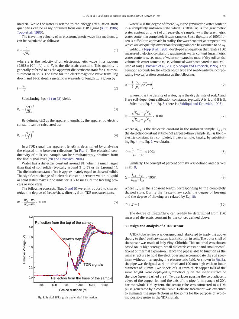
In a TDR signal, the apparent length is determined by analyzingthe elapsed time between reflections (in Fig. 1). The electrical con-ductivity of bulk soil sample can be simultaneously obtained fromthe final signal level (Yu and Drnevich, 2004).

Water has a dielectric constant around 81, which is much largerthan that of soil solids (typically around 3 to 7) or air (around 1).The dielectric constant of ice is approximately equal to those of solids.The significant change of dielectric constant between water in liquidor solid status makes it possible for TDR to measure the freezing pro-cess or vice versa.

The following concepts (Eqs. 5 and 6) were introduced to charac-terize the degree of freeze/thaw directly from TDR measurements.

Φ ¼ wu−wt

wu−wf� 100% ð5Þ

300 600 900 1200 1500 1800

0.0

0.2

0.4

0.6

0.8

1.0

1.2

TDR signals

Reflection from the base of the sample

Rel

ativ

e V

olta

ge (

V)

Scaled distance (m)

Reflection from the top of the sample

Apparent length

Fig. 1. Typical TDR signals and critical information.

where Φ is the degree of freeze, wu is the gravimetric water contentin a completely unfrozen state which is 100%; wt is the gravimetricwater content at time t of a freeze–thaw sample; wf is the gravimetricwater content in completely frozen samples. Since the state of 100% fro-zen is difficult to approach in reality, the water content at temperatureswhich are adequately lower than freezing point can be assumed to bewf.

Siddiqui (Topp et al., 1980) developed an equation that relates TDRmeasured dielectric constant to gravimetric water content (gravimetricwater content w, i.e., mass of water compared tomass of dry soil solids;volumetricwater content, θ , i.e., volumeofwater compared to total vol-ume of soil) (Drnevich et al., 2001; Siddiqui and Drnevich, 1995). Thisequation accounts for the effects of soil type and soil density by incorpo-rating two calibration constants as the following.

w ¼ 1B

ρw

ρd

ffiffiffiffiffiffiKa

p−A

� �ð6Þ

where ρw is the density of water, ρd is the dry density of soil, A andB are soil-dependent calibration constants, typically A is 1, and B is 8.

Substitute Eq. 6 to Eq. 5, there is (Siddiqui and Drnevich, 1995),

Φ ¼ffiffiffiffiffiffiffiffiffiKa;u

q−

ffiffiffiffiffiffiffiffiKa;t

qffiffiffiffiffiffiffiffiffiKa;u

q−

ffiffiffiffiffiffiffiffiKa;f

q � 100% ð7Þ

where Ka, u is the dielectric constant in the unfrozen sample, Ka, t isthe dielectric constant at time t of a freeze–thaw sample, Ka, f is the di-electric constant in a completely frozen sample. Finally, by substitut-ing Eq. 4 into Eq. 7, we obtain,

Φ ¼ La;u−La;tLa;u−La;f

� 100% ð8Þ

Similarly, the concept of percent of thaw was defined and derivedas Eq. 9,

Σ ¼ La;t−La;fLa;th−La;f

� 100% ð9Þ

where La,th is the apparent length corresponding to the completelythawed state. During the freeze–thaw cycle, the degree of freezingand the degree of thawing are related by Eq. 10:

Φþ Σ ¼ 1 ð10Þ

The degree of freeze/thaw can readily be determined from TDRmeasured dielectric constant by the concet defined above.

3. Design and analysis of a TDR sensor

A TDR tube sensor was designed and fabricated to apply the abovetheory to the free/thaw status identification in soils. The outer shell ofthe sensor was made of Poly Vinyl Chloride. This material was chosenbased on its high strength, small dielectric constant and smaller coef-ficient of thermal expansion. Hence the pipe is able to function as themain structure to hold the electrodes and accommodate the soil spec-imen without interrupting the electrostatic field. As shown in Fig. 2a,the pipe was designed as 4 mm thick and 100 mm high with an innerdiameter of 35 mm. Two sheets of 0.09 mm-thick copper foils of thesame height were deployed symmetrically on the inner surface ofthe pipe (green dashed area). Two surfaces passing the two adjacentedges of the copper foil and the axis of the pipe form a angle of 20°.For the whole TDR system, the sensor tube was connected to a TDRpulse generator by a coaxial cable. Delicate treatment was executedto eliminate the imperfections in the joints for the purpose of avoid-ing possible noise in the TDR signals.

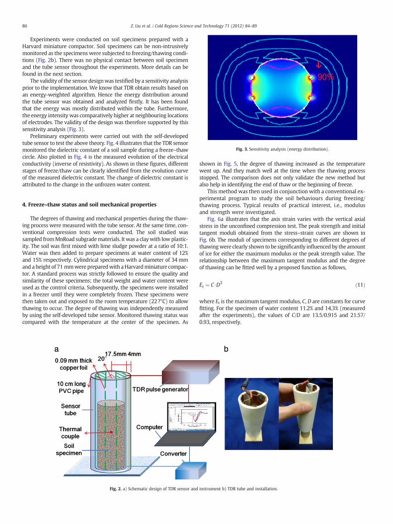
Fig. 3. Sensitivity analysis (energy distribution).

86 Z. Liu et al. / Cold Regions Science and Technology 71 (2012) 84–89

Experiments were conducted on soil specimens prepared with aHarvard miniature compactor. Soil specimens can be non-intrusivelymonitored as the specimens were subjected to freezing/thawing condi-tions (Fig. 2b). There was no physical contact between soil specimenand the tube sensor throughout the experiments. More details can befound in the next section.

The validity of the sensor designwas testified by a sensitivity analysisprior to the implementation. We know that TDR obtain results based onan energy-weighted algorithm. Hence the energy distribution aroundthe tube sensor was obtained and analyzed firstly. It has been foundthat the energy was mostly distributed within the tube. Furthermore,the energy intensity was comparatively higher at neighbouring locationsof electrodes. The validity of the design was therefore supported by thissensitivity analysis (Fig. 3).

Preliminary experiments were carried out with the self-developedtube sensor to test the above theory. Fig. 4 illustrates that the TDR sensormonitored the dielectric constant of a soil sample during a freeze–thawcircle. Also plotted in Fig. 4 is the measured evolution of the electricalconductivity (inverse of resistivity). As shown in these figures, differentstages of freeze/thaw can be clearly identified from the evolution curveof the measured dielectric constant. The change of dielectric constant isattributed to the change in the unfrozen water content.

4. Freeze–thaw status and soil mechanical properties

The degrees of thawing and mechanical properties during the thaw-ing process were measured with the tube sensor. At the same time, con-ventional compression tests were conducted. The soil studied wassampled fromMnRoad subgradematerials. It was a claywith lowplastic-ity. The soil was first mixed with lime sludge powder at a ratio of 10:1.Water was then added to prepare specimens at water content of 12%and 15% respectively. Cylindrical specimens with a diameter of 34 mmand aheight of 71 mmwere preparedwith aHarvardminiature compac-tor. A standard process was strictly followed to ensure the quality andsimilarity of these specimens; the total weight and water content wereused as the control criteria. Subsequently, the specimens were installedin a freezer until they were completely frozen. These specimens werethen taken out and exposed to the room temperature (22?°C) to allowthawing to occur. The degree of thawing was independently measuredby using the self-developed tube sensor. Monitored thawing status wascompared with the temperature at the center of the specimen. As

Fig. 2. a) Schematic design of TDR sensor and

shown in Fig. 5, the degree of thawing increased as the temperaturewent up. And they match well at the time when the thawing processstopped. The comparison does not only validate the new method butalso help in identifying the end of thaw or the beginning of freeze.

This method was then used in conjunction with a conventional ex-perimental program to study the soil behaviours during freezing/thawing process. Typical results of practical interest, i.e., modulusand strength were investigated.

Fig. 6a illustrates that the axis strain varies with the vertical axialstress in the unconfined compression test. The peak strength and initialtangent moduli obtained from the stress–strain curves are shown inFig. 6b. The moduli of specimens corresponding to different degrees ofthawingwere clearly shown to be significantly influenced by the amountof ice for either the maximum modulus or the peak strength value. Therelationship between the maximum tangent modulus and the degreeof thawing can be fitted well by a proposed function as follows,

Et ¼ C⋅DΣ ð11Þ

where Et is themaximum tangentmodulus, C, D are constants for curvefitting. For the specimen of water content 11.2% and 14.3% (measuredafter the experiments), the values of C/D are 13.5/0.915 and 21.57/0.93, respectively.

instrument b) TDR tube and installation.

0 50 100 150 200 250 300 350 400

0

2

4

6

8

10

12

TDR Dielectric Constant

TDR Electric Conductivity

Evo

lutio

n of

Mea

sure

d Q

uant

ities

Evo

lutio

n of

Mea

sure

d Q

uant

ities

Time (minute)

Initialization of freezing

Completely frozen

0 50 100 150 200 250 300 350 400

0

2

4

6

8

10

12

TDR Dielectric Constant

TDR Electric Conductivity

Time (minute)

Completely thawed

a

b

Fig. 4. Measured quantities a) in freezing process; b) in thawing process (Yu et al., 2007).

0.00 0.05 0.10 0.15 0.20 0.250

50

100

150

200

250

300

350

400

450

500

Str

ess

(kP

a)

Axis strain

Sample15-4 (0 min)

Sample15-5 (12 min)

Sample15-6 (24 min)

Sample15-7 (36 min)

Sample15-8 (48 min)

Et

0 12 24 36 480.0

2.5

5.0

7.5

10.0

12.5

15.0

17.5

20.0

22.5

Mod

ulus

(M

Pa)

Time of thawing (minute)

Water content 11.2%

Water content 14.3%

Fitted curve at water content of 14.3%

Fitted curve at water content of 11.2%

0 0.48 0.83 1 1

Degree of thawing

a

b

Fig. 6. a) Results of axis compression test; b) Moduli verse time and degree of thawing.

87Z. Liu et al. / Cold Regions Science and Technology 71 (2012) 84–89

5. Sensor-assisted freeze–thaw analysis in soils

The continuum formation of the mechanical behaviours of geoma-terials consists of the construction of the equation of motion, thestrain–displacement correlation, and the constitutive relationship. Acomprehensive mechanical model based on continuum formation wasestablished to describe the response of soils under freezing condition.The equation of equilibrium (Eq. 12) was introduced in general tensorformat in the first step.

∇⋅ C∇uÞ þ F ¼ 0ð ð12Þ

0 10 20 30 40 50 60 70

-10

-5

0

5

10

15

20

Tem

pera

ture

(D

egre

e C

elsi

us)

Time (minute)

Room temperature

Temperature at the center of specimen

0

10

20

30

40

50

60

70

80

90

100

Deg

ree

of th

aw (

%)

Degree of thawing

Fig. 5. Measured degree of thawing versus time.

where u is the displacement vector, C is the fourth-order tensor of ma-terial stiffness, F is the body force vector.

The strain–displacement equation is

ε ¼ 12

∇uþ ∇uÞT� ih

ð13Þ”

The constitutive equation is

σ ¼ C:ε ð14Þ

where σ is the Cauchy stress tensor, ε is the infinitesimal strain ten-sor, the symbol “:” stands for double contraction.

In order to consider the influence of the thermal field and hydraulicfield on the stress field, the constitutive relationship for porous mate-rials was formulated by:

σ ¼ Dεel þσ0 ð15Þ

whereD is the stiffnessmatrix of soil skeleton andσ0 is the initial stressvector, εel is the elastic strain which can be obtained from the followingrelationship (Liu and Yu, 2010),

ε ¼ εel þ εth þ εtr þ εψ þ ε0 ð16Þ

where,

εth is the strain caused by thermal expansion, [α(T−Tref), α(T−Tref), 0]T;

εtr is the strain caused by the phase change of water, whichwas approximated by [0.03Φθu(1−θu), 0.03Φθu(1−θu),0]T when a unit localization tensor in mixture theory is

0 5 10 15

0.0

0.2

0.4

0.6

0.8

1.0

Deg

ree

of th

awin

g

Suction (MPa)

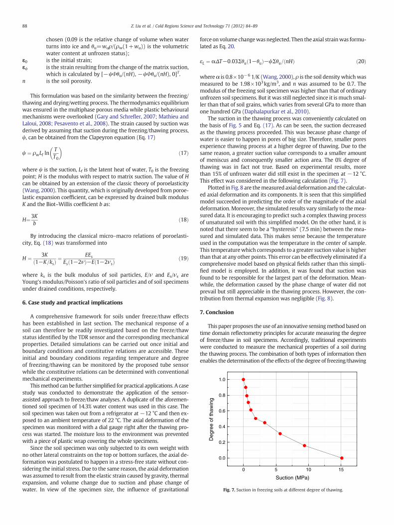
Fig. 7. Suction in freezing soils at different degree of thawing.

88 Z. Liu et al. / Cold Regions Science and Technology 71 (2012) 84–89

chosen (0.09 is the relative change of volume when waterturns into ice and θu=wuρ/(ρw(1+wu)) is the volumetricwater content at unfrozen status);

ε0 is the initial strain;εψ is the strain resulting from the change of the matrix suction,

which is calculated by [−ψΦθu/(nH), −ψΦθu/(nH), 0]T.n is the soil porosity.

This formulation was based on the similarity between the freezing/thawing and drying/wetting process. The thermodynamics equilibriumwas ensured in the multiphase porous media while plastic behaviouralmechanisms were overlooked (Gary and Schrefler, 2007; Mathieu andLaloui, 2008; Pesavento et al., 2008). The strain caused by suction wasderived by assuming that suction during the freezing/thawing process,ψ, can be obtained from the Clapeyron equation (Eq. 17)

ψ ¼ ρwLf lnTT0

� �ð17Þ

where ψ is the suction, Lf is the latent heat of water, T0 is the freezingpoint; H is the modulus with respect to matrix suction. The value of Hcan be obtained by an extension of the classic theory of poroelasticity(Wang, 2000). This quantity, which is originally developed from poroe-lastic expansion coefficient, can be expressed by drained bulk modulusK and the Biot–Willis coefficient b as:

H¼3Kb

ð18Þ

By introducing the classical micro–macro relations of poroelasti-city, Eq. (18) was transformed into

H ¼ 3K1−K=ksð Þ ¼

EEsEs 1−2νð Þ−E 1−2νsð Þ ð19Þ

where ks is the bulk modulus of soil particles, E/ν and Es/νs areYoung's modulus/Poisson's ratio of soil particles and of soil specimensunder drained conditions, respectively.

6. Case study and practical implications

A comprehensive framework for soils under freeze/thaw effectshas been established in last section. The mechanical response of asoil can therefore be readily investigated based on the freeze/thawstatus identified by the TDR sensor and the corresponding mechanicalproperties. Detailed simulations can be carried out once initial andboundary conditions and constitutive relations are accessible. Theseinitial and boundary conditions regarding temperature and degreeof freezing/thawing can be monitored by the proposed tube sensorwhile the constitutive relations can be determined with conventionalmechanical experiments.

Thismethod can be further simplified for practical applications. A casestudy was conducted to demonstrate the application of the sensor-assisted approach to freeze/thaw analyses. A duplicate of the aforemen-tioned soil specimen of 14.3% water content was used in this case. Thesoil specimen was taken out from a refrigerator at −12 °C and then ex-posed to an ambient temperature of 22 °C. The axial deformation of thespecimen was monitored with a dial gauge right after the thawing pro-cess was started. The moisture loss to the environment was preventedwith a piece of plastic wrap covering the whole specimens.

Since the soil specimen was only subjected to its own weight withno other lateral constraints on the top or bottom surfaces, the axial de-formation was postulated to happen in a stress-free state without con-sidering the initial stress. Due to the same reason, the axial deformationwas assumed to result from the elastic strain caused by gravity, thermalexpansion, and volume change due to suction and phase change ofwater. In view of the specimen size, the influence of gravitational

force on volume changewasneglected. Then the axial strainwas formu-lated as Eq. 20.

εL ¼ αΔT−0:03Σθu 1−θuð Þ−ψΣθu= nHð Þ ð20Þ

where α is 0.8×10−6 1/K (Wang, 2000), ρ is the soil density whichwasmeasured to be 1.98×103kg/m3, and n was assumed to be 0.7. Themodulus of the freezing soil specimen was higher than that of ordinaryunfrozen soil specimens. But it was still neglected since it is much smal-ler than that of soil grains, which varies from several GPa to more thanone hundred GPa (Daphalapurkar et al., 2010).

The suction in the thawing process was conveniently calculated onthe basis of Fig. 5 and Eq. (17). As can be seen, the suction decreasedas the thawing process proceeded. This was because phase change ofwater is easier to happen in pores of big size. Therefore, smaller poresexperience thawing process at a higher degree of thawing. Due to thesame reason, a greater suction value corresponds to a smaller amountof meniscus and consequently smaller action area. The 0% degree ofthawing was in fact not true. Based on experimental results, morethan 15% of unfrozen water did still exist in the specimen at −12 °C.This effect was considered in the following calculation (Fig. 7).

Plotted in Fig. 8 are themeasured axial deformation and the calculat-ed axial deformation and its components. It is seen that this simplifiedmodel succeeded in predicting the order of the magnitude of the axialdeformation.Moreover, the simulated results vary similarly to themea-sured data. It is encouraging to predict such a complex thawing processof unsaturated soil with this simplified model. On the other hand, it isnoted that there seem to be a “hysteresis” (7.5 min) between the mea-sured and simulated data. This makes sense because the temperatureused in the computation was the temperature in the center of sample.This temperaturewhich corresponds to a greater suction value is higherthan that at any other points. This error can be effectively eliminated if acomprehensive model based on physical fields rather than this simpli-fied model is employed. In addition, it was found that suction wasfound to be responsible for the largest part of the deformation. Mean-while, the deformation caused by the phase change of water did notprevail but still appreciable in the thawing process. However, the con-tribution from thermal expansion was negligible (Fig. 8).

7. Conclusion

This paper proposes the use of an innovative sensingmethodbased ontime domain reflectometry principles for accurate measuring the degreeof freeze/thaw in soil specimens. Accordingly, traditional experimentswere conducted to measure the mechanical properties of a soil duringthe thawing process. The combination of both types of information thenenables the determination of the effects of the degree of freezing/thawing

-5 0 5 10 15 20 25 30 35

0.0

0.2

0.4

0.6

0.8

Measured: Total

Calculated:

Total Total(no hysteresis)

Suction Phase change

Thermal expansion

Axi

al d

efor

mat

ion

(mm

)

Time (minute)

Hysteresis

Fig. 8. Axial displacement and its components.

89Z. Liu et al. / Cold Regions Science and Technology 71 (2012) 84–89

on the soil mechanical properties. Moreover, suction stemming from thethermodynamic equilibrium at the ice–water interface has been relatedto temperaturewhich canbemeasuredwith thermocouples. A theoreticalframework for freeze–thaw analysis in geomaterials was therefore estab-lished in order to utilize the aforementioned information from sensordata. This sensor-assisted analysis approach intends to serve as a holistictechnique for the freeze/thaw analysis in soils and other geomaterials. Acase study was presented to demonstrate the implementation of this ap-proach. This preliminary investigation not only validated the theoreticalframework but also confirmed the potential of the technique in practicalapplications. The technology and analysis procedures will be further re-fined in subsequent studies. This will not only help study the complex

soil behaviours during freeze/thaw process, but will also provide impor-tant decision-support for implementing preventative maintenance strat-egies for infrastructure in cold regions.

References

Daphalapurkar, N.P., Wang, F., Fu, B., Lu, H., Komanduri, R., 2010. Determination of Me-chanical Properties of Sand Grains by Nanoindentation. Experimental Mechanics51 (5), 719–728.

Drnevich, V.P., Siddiqui, S.I., Lovell, J., Yi, Q., 2001. Proceedings TDR 2001– Second Inter-national Symposium and Workshop on Time Domain Reflectometry for InnovativeGeotechnical Applications. Northwestern University, Evanston, IL.

Frost Resistivity Probe User Guide. Minnesota Department of Transportation. (1996)Gary, G., Schrefler, B.A., 2007. Analysis of the solid phase stress tensor in multiphase

porous media. International Journal for Numerical and Analytical Methods 31,541–581.

Klut, E.A., 1986. Methods of Soil Analysis, Part 1, Physical and Mineralogical Methods,2nd edition. Wiley Periodicals, Inc, Madison, Wisconsin.

Konrad, J.M., 1994. Canadian Geotechnical Journal 31, 223–245.Liu, Z., Yu, X., 2010. GeoFlorida 2010: Advances in Analysis, Modeling & Design. ASCE

Geotechnical Special Publication, Vol. 199, pp. 157–164.Mathieu, N., Laloui, L., 2008. International Journal for Numerical and Analytical

Methods 32, 771–801.Neaupane, K.M., Yamabe, B., 2001. Computers and Geotechnics 613 Vol..Nishimura, S., Gens, A., Olivella, S., Jardine, R.J., 2009. Geotechnique 59, 159–171.Pesavento, E., Gawin, D., Schrefler, B.A., 2008. Acta Mechanica 201, 313–339.Roberson, R., Siekmeier, J., 2000. Transportation Research Board, Washington, DC, pp.

108–113.Siddiqui, S.I., Drnevich, V.P., 1995. Report No.: FHWA/IN/JTRP-95/9, Indiana Depart-

ment of Transportation - Purdue University.Topp, G.C., Davis, J.L., Annan, A.P., 1980. Water Resources Research 16, 574–582.Wang, H.F., 2000. Theory of Linear Poroelasticity with Applications to Geomechanics

and Hydrogeology. Princeton University Press, USA.Yu, X., Drnevich, V.P., 2004. Journal of Geotechnical and Geoenvironmental 130, 922.Yu, X.B., Liu, N., Gonzalez, J., Yu, X., 2007. Proceedings of Transportation Research Board

Annual Conference.Yu, X., Zhang, B., Liu, N., Yu, X., 2010. J. of Adv. Civ. Eng. Vol. 2010. Article ID 239651, 10

pages. doi:10.1155/2010/239651.