combining loss aversion with the standard economic model

2012

Name: Daan Gouka

Thesis: Economie&Bedrijfseconomie

(8 ECTS)

Supervisor: Aurélien Baillon

School: ESE, Erasmus University

Rotterdam

2-7-2012

Combining loss aversion with the standard economic model.

of 39

Table of contents

Table of contents ………………………………………………………….......2

Preface ………………………………………………………………………...3

1. Introduction ………………………………………………….…..4

2. Review of the standard micro economic model ………………...6

2.1 SEM, budget constraints and indifference curves …...……...5

2.2 Practical applications ……………………………………..9

3. Review of important behavioral economic theories …………...11

3.1 Prospect theory and loss aversion ……………………..11

3.2 Status quo bias ………………………………………...15

4. Implementation of loss aversion in SEM ……………...... …….16

4.1 Reference-dependent model …………………………..16

4.2 The interpretations of the loss aversion coefficients ….21

4.3 R-D model with stationary reference points …………..20

4.4 R-D model with changing reference points …………...26

4.5 A SEM example with reference points ………………..29

5. Experiment ……………………………………………………..32

6. Discussion ……………………………………………………...34

7. Conclusion ……………………………………………………..35

Appendix …………………………………………………………………….37

References …………………………………………………………………...38

of 39

Preface

When I followed the micro economic courses in my first and second years of my study, I was

fascinated by the explanatory power on behavior many of these micro models seemed to have. My

first feeling was that it was all very interesting, however when I passed these courses, a feeling started

to grow on me that I would not be able to shake off, a feeling that these mathematical models would

never really capture an actual decision making progress. When I observed the actions and decisions of

others and myself, I observed so much irrational behavior that I actually started to wonder why I spend

so much time studying theory that was not applicable. Of course my micro teachers did not sell me

some fairy tell that these models did not have limitations. However, the fact that a bachelor student

spends months of their time studying these models and spends hundreds of euro‟s on mathematical

micro economic books should in my opinion mean that we actually get taught practical valuable

methods.

The behavioral economic courses where the first courses that actually introduced principles that really

covered the human psyche and really formed the already present ideas in my mind. But instead of

building forth on micro economy, the theory was based on experiments and formed its own theory. I

started to recognize patterns of loss aversion and status quo bias in many, many elements of day-to-

day life and confronted many micro economists that their theoretical work and conclusions missed

these elements.

In this thesis I want to take the basic micro economic model and improve them with one or more

behavioral economic ideas. I spoke to micro economists and their opinion on behavioral economic

bothered me. I want to counter the micro economists arguments against the behavioral economic field

by showing the importance what can be done by a merging of the two field, and to convince people

that behavioral and micro economics should not be different fields but behavioral economics should be

the layer on top of micro economics to complete it. I want to help build the layer that actually brings

the micro economic field to the next level and deals with the many irrationalities human decision

making has. Even if I do not succeed merging the models, I want to at least show the problems I faced

and most importantly inspire other people to expand the behavioral economic field.

After writing this thesis, I realize now that it is much harder to combine the models than I thought it

would be. I faced a lot of problems, and I want to thank my coordinator, dr. Baillon, for helping me

through the progress. Although it was sometimes hard, I did learn a great deal about behavioral

economic models. Enjoy reading.

Daan Gouka

of 39

1. Introduction

In this thesis, I will be studying the standard micro economic model of rational decision making, the

behavioral economic theories of loss aversion and reference points and how these two theories (can)

interact.

When first year economics students are lectured in basic micro economic, the standard economic

model of rational decision making is one of the first lectures and it covers how rational agents make a

choice between two goods when they are restricted by a budget. Newer studies in behavioral

economics have formed theories of loss aversion and how a reference point can influence decision

making. Although there are successful experiments backing up these behavioral economic theories, the

standard economic model (without additions of these behavioral theories) still remain the corner stone

of the micro economic curriculum.

I believe micro economics could be a far more advanced field when irrationalities and these behavioral

phenomena were actually incorporated in the consumer decision making models. I hope this thesis will

add value to science by showing exactly what creates the gap between standard micro economics and

behavioral economics and see which steps are to be taken to merge the two fields to have more

realistic predictions. To use a metaphor, I believe that behavioral economics is potentially a gold layer

on the micro economic engine of rational decision making, and that these theories enhance our ability

to predict (consumer) decision making. I think it is important for policymakers and managers to

understand that they cannot always rely on rational models and I believe that if decisions are made

with rational micro economic models, behavioral models should be integrated in the decision making

progress as well. The economic problems we faced and still deal with all over the world are examples

of why it is important to also look at “real world” irregularities, anomalies and other (psychological)

phenomena that compromise realistic predictions of current rational (micro) economic models.

My research question in this thesis is: "How do loss aversion and reference point theories change the

first step of micro economic analysis and how do these behavioral economic models differ from the

standard economic model."

My thesis is build up in the following way:

After this introduction, in section 2 I describe how the standard micro economic model works.

Indifference curves are combined with a budget constraint to find an optimal bundle when we assume

the rational decision making progress. I will give practical examples and implications. Next, in section

3, I will describe the important theories behind loss aversion, and some powerful examples of how we

can observe loss aversion in day-today decision making. Part 2 and 3 of my thesis can be seen as

theory review.

of 39

In part 4, I will try to incorporate both the idea of loss aversion into the standard economic model and

see how the model changes exactly. Section 4 will also be a detailed section on the differences

between the SEM and the model used to incorporate loss aversion and a report on which practical

problems I encountered trying to incorporate the loss aversion into the SEM. I use a reference-

depended utility model (Tversky & Kahneman 1991) to show what happens when loss aversion is

introduced into a decision model. I used practical examples to show the different predictions the two

models give. Next, there will be a discussion part of my thesis, where I will present more ideas on

research that still could be conducted to really mold both models into one model, that the task I

originally set out for, but was unfortunately was too difficult for me to pull off at this time. Also I will

discuss some elements that can be improved and I will critique my own work.

The main part of this thesis ends with the idea for an experiment to test whether real findings support

either the principles for the standard economic model or the theory of loss aversion. Finally, there will

be a conclusion with all my findings and the answer to my main research question, an appendix (where

I clarify which calculations I used to shape the graphs and curves) and the reference list.

of 39

2. Review of the standard micro economic model.

In the first part of my thesis I will describe the general theory of the standard micro economic model

for consumer decision making, or more shortly the SEM (standard economic model).

2.1 SEM, budget constraints and indifference curves

The micro economic theory I am reviewing in this thesis is the theory of rational consumer choice.

Rational agents enter a market of goods, and while prices are fixed (and given) they allocate their

income to maximize their personal utility (by consuming the goods). Their income is described by the

budget constraint. The budget constraint describes every possible combination an individual can buy

of two types of goods (given a fixed income). For instance food and shelter, good x and good y, or

good x and the composite good y.

The consumer‟s budget line is only one part of graphing the rational consumer choice. Mapping the

preferences of the economic agent is another vital part. We can capture the preferences of an agent by

mapping an indifference curve. An indifference curve is a set of consumption bundles, among which

the economic agent is indifferent. We speak of indifference when the individual is examining different

consumption bundles, and he would receive the same utility from every consumption bundle in

question. Simply said, the individual does not care which of these allocation of goods he consumes, if

they are on the indifference curve. Every individual has of course different tastes and preferences and

therefore every individual has a different indifference curve. In figure 1 I displayed two Cobb-Douglas

indifference curves. Cobb-Douglas refers to the way the utility function is build up, I will clarify this

later.

of 39

Figure 1

In the SEM, the agent is indifferent about which bundle on the indifference curve he currently

possesses. That means in theory, the individual is indifferent whether the consumer has the choice

between points A and B and is also indifferent if he has to choice between points X and Y. This is

because points A and B are on the same indifference curves and so are points X and Y. Any of these

(or other) consumption bundles on this line will give him the same total utility.

The standard economic model states 4 important properties of preference ordering. I will shortly

discuss these stylized facts of the standard economic model.

1. Completeness, the agent has ordered all possible combinations of goods. If we take this

property literally, it is never satisfied but it is meant to rule out certain combination that are

not included in the preference ranking, but are actually preferred over other bundles.

2. Monotonicity property (more-is-better). Higher indifference curves are preferred over curves

that are lower in the graph. It is implied that a higher quantity of a good translates to a higher

utility.

3. Transitivity, a property that is easily violated. If A>B and B>C then A>C. A more clear

example, if Fanta is preferred above Pepsi and Coca Cola is preferred above Fanta. Then it is

implied that Coca Cola is preferred above Pepsi. This property is violated when indifference

curves intersect each other

4. The allocation is prone to diminishing rates of marginal substitution. This means that the

higher the quantity consumed of a good, the more of that good you are willing to trade in for a

x₂

x₁

Cobb-Douglas indifference curve

Low utility High utility

Y

X

A

B

of 39

quantity of another good. For example if we have a huge amount of good x, the marginal

utility of an extra unit of good x has diminished so we want to trade a big amount of good x

for only a small increase in good y.

In the last property, I mentioned the marginal rate of substitution. Something I will henceforth call the

MRS. The MRS is the rate of which the agent is willing to trade in good y for one quantity of good x.

(If good y is on the vertical axe and good x is on the horizontal axe). The MRS is different at every

point on the indifference curve, and is equal to the slope of the line in that point. Because the curves

are convex, the marginal rates of substitution decrease as the quantity of good x increases and increase

as the quantity of good y increases.

The best feasible bundle is the point in which the budget line still reaches the highest possible

indifference curve. In the best affordable bundle, the utility of the consumer is being maximized under

that budget restriction. If the indifference curve is not tangent with the budget line, the bundle is

simply not affordable. In the following figure, the best feasible bundle is showed at point A (25,50)

Figure 2

A

0

10

20

30

40

50

60

70

80

90

100

0 10 20 30 40 50 60 70 80 90 100

x₂

x₁

Indifference curve and budget line

Indifference curve Budgetline Point A

of 39

This standard economic model ignores behavioral models that explain the sunk costs fallacy and cover

theories that explain cognitive biases1. It presumes the economic agent is a „homo economicus‟, who is

looking for personal utility maximalisation while making rational decisions. The theory does not say

the model can predict choice behavior, because there is still a big discussion whether people are

rational decision makers, however rational decision making is often viewed as an ideal. A normative

goal (we all want to act as rational as we can possibly act).

The SEM states that the agent we are looking at has a utility function2 of U(x,y), if the indifference

curve is actually composed of the goods x and y, as I described. I also mentioned Cobb-Douglas utility

functions, without going into this deep, I want to shortly clarify this. The Cobb-Douglas utility

function is a utility function where the quantities of good x and good y are subject to a power, and

therefore have diminishing marginal utility as shown in figure 1. Diminishing marginal utility is an

important principle of indifference curves in the SEM, so it is important for SEM indifference curves

to have this element. Basically, a Cobb-Douglas utility function has the shape of

x y x y

This way, we can model diminishing marginal utility, and SEM indifference curves.

2.2 Applications of the SEM

I also want to show practical applications of the rational decision making model. We can use the SEM

to explain how rational decision making will react to for example changes in preferences, prices or

budgets.

Let us take an example of food stamps3. We can think about whether it makes a difference if the

government has a social program where it gives people with a low income food stamps, instead of

money to support them. When the government increases the income of the individual with 100 euro‟s,

the entire budget line of the individual will shift to the right, for the individual can spend the extra

stimulant on the primary good x (food) or the compound good y (all other goods).

However when the alternative of food stamps is chosen, only the range of good x (food) is being

extended with 100 euro‟s and the compound good y (all other goods) stays at the old intersection with

the y axis. In this case, the budget line is only shifted to right for good x, but remains exactly the same

1 Cognitive biases are patterns of deviation in judgment that can occur in decision making, leading to decisions

that can be viewed as irrational and not in accordance with the SEM and rationality. Phenomena that are relevant

to this thesis are explained in section 3. 2 The utility function covers the amount of utility an agent experiences. In this example, his or her utility is

derived by the quantities of goods x and y possessed. 3 Micro economics and behavior, Robert H. Frank, chapter 3 Rational consumer choice, p.73 example 3.4

of 39

for the range of compound good y. At the point where the food stamps run out, there is a kink in the

budget line and the new budget resumes there with the form of the old budget line.

In the SEM, the indifference curve will intersect the old and new budget lines at exactly the same

point when the economic agent spends a greater amount on money on food than the amount of

distributed food stamps, which will be the case in a lot of practical situations. When that is the case,

both alternatives will give the same consumption pattern. He will actually just spend the money he

saves with the food stamps on other goods. This can be important to know for the government because

a plan with food stamps will cause the government extra work and costs, although the behavior of

people is not altered.

Another practical important facet I need to mention is the way the optimal bundle changes when there

is a change of prices. The change of optimal bundle is caused by the income effect of the change and

the substitution effect of the change. When the prices are changed of the individuals budget gets

altered, there is an income effect in the form that the person can buy more or less goods in the new

situation compared to the previous situations. It is important to understand that next to this main effect,

there is a substitution effect that covers the change in opportunity cost. For example when wages rise,

a person can earn more money by working the same amount of hours so he can afford it now to work

less. However, a change in the wage for work means that leisure becomes more expensive than before

so the substitution effect has a negative effect on the increase of leisure time because the opportunity

cost of leisure has risen. Therefore when wages rise, a new budget line will be formed and there is

possibly a new optimum.

Because every situation is different, it is hard to give a rule of thumb on how the optimum increases

when there is a wage change with the SEM. But what I can state is that is that the substitution effect of

a wage increase will make people work more (take less leisure) because the price of leisure has gone

up and the income effect will make people work less (take more leisure) because the person now needs

less work hours to earn a satisfying level of income. It depends on multiple factors (for example, the

wage increase, preferences and the individuals utility function) whether the income or the substitution

effect dominates the new situation. It is for example a possibility that people will work less because of

a great income effect because people now earn more money. It depends on the situation.

of 39

3. Review of important behavioral economic theories

"I hate to lose, more than I like to win."

- Larry Bird, retired NBA basketball player, 1998

3.1 Prospect theory and loss aversion

To implement loss aversion in consumer decision making, we must first understand where loss

aversion comes from. Loss aversion is part of Prospect Theory (PT), a behavioral economic theory

composed by Daniel Kahneman and Amos Tversky in 1979 to take a more realistic and psychological

look at the standard economic decision model. In this thesis I will cover the basic elements of prospect

theory, and try to incorporate as many of them in standard economic consumer decision models.

Before the emergence of behavioral economics, bounded rationality was one of the first theories that

covered the absence of rationality of economic agents in certain situations. Bounded rationality was a

concept, introduced by Herbert Simon to explain that economic agents in the real world, are prone to

imperfect information and a limited ability to compute the right decision while in a complex and

dynamic decision environment.4 It shows the boundaries agents have when dealing with decisions

under risk and uncertainty, and that they are actually never truly rational. Also the use of heuristics and

rules of thumb and emotions can become important in decision making, which can lead to irrational

and controversial decision making. During the last fifty years, models and theories have been

developed to explain why people do not act the way a perfectly rationally individual should act.

Prospect theory is one of the most popular and influential theories that has been developed to give a

more realistic outlook on (consumer) decision making.

I will shortly discuss the important paradigms of prospect theory.

1. People are prone to subjective probability weighting. They weigh small probability events

(with high outcomes) too high. Because of that, they overweigh events with a small chance of

occurring.

2. Not absolute gains and losses in utility are important, but relative gains and losses when being

compared to a reference point. The reference point is the bundle an economic agent is

currently consuming. A gain or loss will cause a change in utility, but only relative to the

reference point. Also, this change will over time shift the reference point to a new point.

4 Wilkinson, N. (2008). An introduction to behavioral economics. Chapter 3. Page 98

of 39

3. People are prone to loss aversion, which means people prefer avoiding a loss to acquiring a

gain. For example, losing a certain amount of money will generate a bigger amount of

negative utility than gaining that same amount of money would generate a positive amount of

utility.

4. Framing effects. Decisions can change when the situation or question is constructed

differently. A more positive question can cause a different outcome than a negative question,

even though both questions describe the same sets of circumstances.

Let us take a closer look at loss aversion. It is very interesting to look into the fact why we are actually

prone to this aversion to losses. The most logical explanation (at this moment) for this phenomenon

can be found in evolutionary psychology. S. Pinker5 states that gains of utility and goods can improve

chances of survival and replication, however losses can have much more devastating results. Let us

think of a situation thousands of years ago, in early tribal societies, when humans did not have

technologies to store foods, water and other goods. If one of our tribal ancestors would have a huge

quantities of food, he was not able to store all these goods so he could survive the coming months.

Also, it is not possible to consume huge quantities now and be satisfied for a week because our body

can only process a certain amount of food and once you are satisfied, the next day you would have the

need to satisfy your thirst and hunger again. However, if he lost a (small) quantity of food and is not

able to satisfy his need for food, he could starve to death. Humans have lived and reproduced

thousands of years. For the biggest part, only the humans who mastered the qualities to survive and

reproduced, have actually done so, and passed on those genes. Because the human physiology needs

nourishment almost every single day, losing precious food and water was more of a loss, than the

gains of (big) quantities of foods and water (which could not be consumed now because the human

intake of nutriment is not building up but is satisfied at a certain point and) which could not be stored.

It is these 'instincts' that have been passed on over thousands of years.

Experimental studies have shown that the negative utility of a (small) loss is approximately 2 to 2.5

times as big as the positive utility of a (small) gain.6 The direct consequence of this fact would be, if

we would look at the utility function of an individual, a kink in the function at the point he is currently

consuming (the status quo). For at that point, he is more afraid to lose utility then to gain more utility.

A very clear example of loss aversion is for example when a person is spending a night in the casino

and there are two situations that might occur. The first one is that he wins for example 100 euro's and

leaves, and he will experience a utility gain according to a 100 euro gain of wealth. The second

situation is that he first gains 130 euro's, then loses 20 euro's and then leaves. A loss averse individual

5 “Pinker, S. (1997). How the mind works”

6 Bowles S. Microeconomics, Behavior, Institutions and Evolution.(2006) Chapter 3, page 104.

of 39

might have a higher total utility in the first situation, although the total wealth gain was higher in the

second situation.

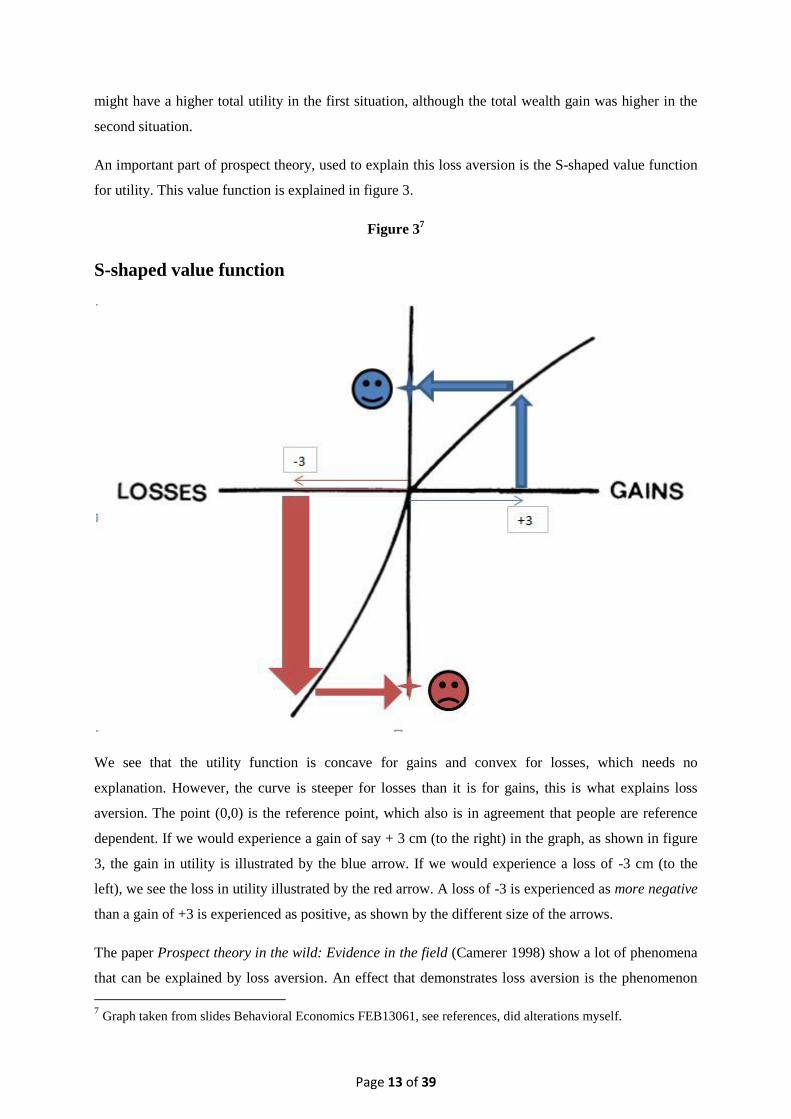
An important part of prospect theory, used to explain this loss aversion is the S-shaped value function

for utility. This value function is explained in figure 3.

Figure 37

S-shaped value function

We see that the utility function is concave for gains and convex for losses, which needs no

explanation. However, the curve is steeper for losses than it is for gains, this is what explains loss

aversion. The point (0,0) is the reference point, which also is in agreement that people are reference

dependent. If we would experience a gain of say + 3 cm (to the right) in the graph, as shown in figure

3, the gain in utility is illustrated by the blue arrow. If we would experience a loss of -3 cm (to the

left), we see the loss in utility illustrated by the red arrow. A loss of -3 is experienced as more negative

than a gain of +3 is experienced as positive, as shown by the different size of the arrows.

The paper Prospect theory in the wild: Evidence in the field (Camerer 1998) show a lot of phenomena

that can be explained by loss aversion. An effect that demonstrates loss aversion is the phenomenon

7 Graph taken from slides Behavioral Economics FEB13061, see references, did alterations myself.

of 39

called the disposition effect (Shefrin and Statman 1985). The disposition effect states that investors are

too eager in selling stocks that are climbing in value and are too reluctant on selling stocks that were

losing value. Loss aversion makes it difficult for economic agents to accept the loss and sell the

declining stock, while on the other hand being too quickly to sell rising stocks before the increase

comes to a halt. The need here for not wanting to lose, is bigger than the need of making profit.

Another effect very similar to this one is the endowment effect where the owner of a good puts a

higher value on the good than the potential buyer (or person who does not own the good). In other

words, selling prices are said to be higher than buying prices. The true reasons for this fact is debated

on by economists and psychologists alike, but loss aversion seems to be one of the possible

explanation. This view is shared in the paper of Kahneman, Knetsch and Thaler (1990) that included

the famous mug experiment. One group of people were given mugs and they valued these mugs as 2 to

3 times higher than the people who were buying the mugs. The 'willingness to sell price' was higher

than the 'willingness to buy' price. Even among economists, there are actually multiple views on this

effect, it is possible to explain this phenomenon while using the SEM but also to explain this with the

help of PT and loss aversion.

Let us look at this effect with the SEM. When the owner of a good goes from quantity one, to quantity

zero, the marginal utility of that good rises. It is like when our quantity of goods rises, the marginal

utility diminishes. A more practical example is when you are eating a sandwich and you have one

bottle of Fanta, the marginal utility of the second bottle of Fanta is lower when you do not have a

bottle at all and you want to determine the marginal utility of 1 bottle at that moment when you have

nothing to drink. This however does not yet explain why the owner of the bottle of Fanta in that

moment values the drink higher than the buyer and non-owner, however this element of the

endowment effect was interpreted through the SEM in the paper Resolving Differences in Willingness

to Pay and Willingness to Accept (Hahneman 1991). Hahneman argued that the difference of wealth

between to bundles on a low and high indifference curve was smaller when moving up a bundle than

moving down a bundle. This is because he used different points on the indifference curve to measure,

however that would not matter for the result because the individual is supposed to be indifferent on all

points of the indifference curve. The fact that he could prove this meant that even in the SEM there

can be an endowment effect through the income and substitution effect I mentioned in part 2.2.

Let us bring PT in this example. Because the person with the sandwich and the Fanta is at his

reference point he would rate losing the bottle Fanta as more negative than the person without would

positively rate gaining the bottle of Fanta. This can be interpreted as loss aversion, because the person

who owns the good will need a higher compensation for giving up the utility of the good than the

buyer is willing to pay as the S-shaped value function predicts. The difference between these two

of 39

values, the value of the owner and the value of the buyer can be induced by loss aversion and creates

an endowment effect.

Another important effect caused by loss aversion is the equity premium on stocks. A study of Mehra

and Prescott (1985) showed that the premium that compensated the risk on stocks was relatively very

high and that the owners of the stocks had to be incredibly risk averse. A more recent study of Thaler

and Benartzi (1997) explained that this premium was caused by loss aversion because stocks had

higher a risk of losing their value compared to bonds and had a higher probability to cause a loss of

wealth on the short run for investors. The aversion for this loss causes the equity premium on stocks.

Another interesting phenomenon is the fact that price elasticities were shown to be asymmetric for

increases and decreases of prices. Loss aversion causes people to dislike a increase in prices more than

they would enjoy a lowering in prices, and these outcomes have been found in experimental cases

done by Putler in 1992 with prices of eggs. It is essential for micro and macro policy makers to be

aware of this asymmetry because people might for example value an increase of the value added tax

differently than a decrease of the value added tax. According to the S-shaped utility function and loss

aversion, an increase of the value added tax will arguably cause a bigger negative shift of utility than

the same decrease of the value added tax will cause a positive shift in utility.

3.2 Status quo bias.

This combination of loss aversion and the endowment effect are to big drivers of the status quo bias.

The status quo bias is the phenomenon (observed by Daniel Kahneman8, inter alia) that people have a

tendency to prefer their current behavior or consumption bundle. They prefer their status quo (state

where they are in now) over a different situation, even though the new situation can bring the agent

higher utility. A clear example of this bias is that people often stay at their default retirement plan,

even though they have the option to change to a retirement plan that is financially better for them.

People are afraid that if they switch their consumption bundle or behavioral pattern, they will actually

regret the decision or experience firsthand that the switch is not as positive as it looked on first sight.

In other words, they are more afraid of the potential loss of the change than they are attracted to the

potential gain of the change, a form of loss aversion, and therefore important to mention.

8 Kahneman, D., Knetsch, J. L. & Thaler, R. H. (1991). Anomalies: The Endowment Effect, Loss Aversion, and

Status Quo Bias.

of 39

4. Implementing loss aversion into the standard economic model

In part 2 and 3 of this thesis I have described the theory of the SEM and the behavioral economic

concept of loss aversion. In part 4 I am actually looking into the possibility of merging the SEM with

loss aversion.

4.1 A reference-dependent model

Before we can draw an indifference curve, we map the preferences of the economic agent. The

individual states at what quantities of goods x and y he is indifferent. For example the agent can be

indifferent between 'holiday spending' (good x) of 600 euro's and a composite good y (all other

spending) of 2000 euro's and a holiday of 400 euro's and a composite good y worth of 2500 euro's. It

depends on the marginal rate of substitution, the rate at which the agent is willing to swap the two

quantities of goods. In this example, the agent is willing to lower his holiday spending with 200 euro's

when his composite good y gets compensated with 500 euro's. I have discussed this already in part 1

so I will not repeat this, I want to try to incorporate loss aversion in this example through the use of a

reference point, a status quo.

When the economic agent is mapping his preferences, the model is assuming he is measuring the

utility of each bundle rationally and all bundles provide him with equal utility. We have established

that when the quantity of good x is very high (implying that the quantity good y is relatively low), the

marginal utility of good y is very high also because of the law of decreasing marginal utility. However

loss aversion dictates that if an agent is actually rating the loss of a bundle differently than a gain in

that bundle of goods. Because in the SEM with the marginal rates of substitution, loss aversion is

currently ignored completely, I am looking for a model that can actually change the forms van

indifference curves to model decision making with loss aversion better. In other words, losses have to

be valued quite differently than losses.

In their paper of 1991, Amos Tversky and Daniel Kahneman already tried to implement loss aversion

in a choice model. In this part of my thesis I will describe this model and eventually try to simulate

my own findings according to this model.

While the micro-economic Coase Theorem asserts that initial entitlements and allocations like

reference points (except for transaction costs) do not affect rates of exchange, I have already

mentioned (and there is substantial evidence) that rates of exchange can differ when we view that good

as a loss or a gain.

When the economic agent is mapping his preferences, the SEM is assuming he is measuring the utility

of each bundle rationally and all bundles provide him with equal utility. However, in behavioral

of 39

economics, it is debated if agents can actually rationally value the utility they will receive (more

specifically, rating losses differently than gains). We have established that when the quantity of good x

is very high (implying that the quantity good y is relatively low), the marginal utility of good y is very

high also because of the law of decreasing marginal utility. However the status quo bias dictates that if

an agent is actually consuming one of the (many) possible consumption bundles, he has a natural

dislike for actually changing (losing quantities in) this bundle. That means when he is mapping his

preferences, his preferences are actually different than when he is actually consuming one of those

bundles. The current SEM can be used to graphically show the preferences and choice of the agent

before he actually acquires the bundle of goods. The model that Tversky and Kahneman have created

tries to divert from the SEM and introduces the phenomenon that the individual actually experiences a

bigger utility loss when he loses quantity compared to his status quo, than he would gain utility when

the same amount of this good would be increased instead of lost.

When we introduce the reference point r, we have to keep in mind that advantages and disadvantages

relative to point r are weighed differently. More to the point, disadvantages (losses) loom larger than

advantages (gains).

The next thing is diminishing sensitivity. The diminishing sensitivity states that deviations that are

very far away from the reference point have a smaller effect than deviations close to a reference point.

It is comparable to the assumption of diminishing marginal utility but it now, it covers the reference

point. Tversky and Kahneman mention the similarities between diminishing sensitivity and

diminishing marginal utility, but also mention the fact that both ideas have a different founding.

I will now describe the mathematical equations of the model. I use somewhat different equations to

make it more understandable but the essence remains the same:

₁ ₂ ₁ ₂

₁

₁ ₁

₁

The model describes that when the utility of good x (u(x)) is above the utility of the reference point r

the extra utility is simply the gain that is being described. However when the utility of good x is below

of 39

the utility of reference point r, a factor is introduced in the model to make the utility change more

extreme. The term is the loss aversion factor, which makes the effect on final utility stronger for a

loss than a utility gain (even if the gain and loss are equal in absolute value). Both types of goods (x₁

and x₂) can have different loss aversion factors and different reference points.

Say we have a simple situation where this utility curve has following assumptions:

₁ ₂ ₂

₁ and ₂

These assumptions state that we have a utility curve in the simplest form. The first assumption states

that the total utility of both goods ₁ ₂ is simply the total individual utility of both goods

combined. The second assumption states that the utility that is derived out of good ₁ and ₂ equals

the quantity of that particular good. There is no conversion of quantity to personal utility, though it

would not be a problem using such coefficients in this model. Also note that in this model,

diminishing marginal utility have not been introduced.

So let us work out these formulas by creating two indifference curves with the good x₁ and x₂ and see

how they can differ compared to the reference point r (r₁,r₂). In our example, we use 2 different values

for . For x₁ we use a ₁ value of 0.5 and for x₂ we use a ₂ value of

.

This means that the behavior of loss aversion in an individual is different for both goods. An essential

part of this model is the reference point r. In my example of figure 4, I have chosen for reference point

r(5,5) so good x₁ has a quantity of 5 and good x₂ has a quantity of 59. Any utility increases from this

reference point will just be as big as that extra utility of the goods increased. However, if the quantity

of one of the two goods goes under the reference point, that will be valued as extra harsh because of

the loss aversion coefficient .

9 The fact that the reference point r is not on the current budget line can be interpreted by assuming that for

example, the reference point is a prediction of the future (and a new budgetline). In parts 4.3 and 4.4 we will see

reference points on the budget lines.

of 39

Figure 4

To explain this model more accurately. One can split this graph in 4 pieces, with the reference point

r(5,5) in the center. The bottom left part, the bottom right part, the upper left part and the upper right

part.

In the bottom left part, the part with the quantities (0,..,5) for both x₁ and x₂ are a loss in both goods

compared to the reference point r. In that point, both factors of are at work when deriving new

utility.

In the upper left part, we find the values of (0,...,5) for good x₁ and (5,...,10) for good x₂. So in that part

of the curves, the loss aversion coefficient ₁ is only active on good x₁ because quantities (0,...,5) are a

loss compared to the reference point of 5.

In the bottom right part, we find the values for (5,,.14) for good x₁ and (0,..5) for good x₂. It is no

surprise that only the ₂ coefficient now works on good x₂ because of the loss in quantity compared to

the reference point of 5.

5

0

1

2

3

4

5

6

7

8

9

10

11

12

13

14

0 1 2 3 4 5 6 7 8 9 10 11 12 13 14

x₂

x₁

Indifference curves in the R-D model

5 total utility -5 total utility reference point

of 39

Finally, the upper right part of the graph consists of quantities higher than 5 of both goods. Because

this is a gain compared to the reference point r(5,5), the two loss aversion coefficients are not at work

in this part of the graphs.

We can see in the graph, that the slope of the indifference curve is different when we have a loss in

different goods, this is because the loss aversion coefficients is different for both goods. Of course,

the shape of the individual indifference curve is not unusual, but in the SEM, the convex shape is

actually due to the law of diminishing law of marginal utility, not loss aversion. In this model

however, the convex shape is caused my loss aversion because of the different factors of for both

goods, and the law of diminishing marginal utility has been left out. In all 4 sectors in this example,

there are different marginal rates of substitution. Of course, like I explained, this is normal in standard

micro-economics, however in this studies these differences in each MRS is caused by diminishing

marginal utility, not loss aversion.

We defined the MRS as the absolute value of ₂

₁. It gives the quantity of x₂ to compensate for a

loss of 1 good x₁.

Because the two coefficients actually explain the shapes of these indifferences curves in this model,

we can write ₁ and ₂ as a function of the MRS.

In the upper right part of the graph, every change is a gain compared to the reference point so the MRS

is 1. ₁ and ₂ are the only factors influencing the trade off, and because all changes are gains, the

MRS is not influenced by these factors.

In the upper left part, the MRS equals

, in the example of figure 4, the MRS here equals 2

In the bottom left part, the MRS equals

, in the example of figure 4, the MRS here equals

In the bottom right part, the MRS equals , in the example of figure 4, the MRS here equals

We now have a model that derives different indifference curves while the consumer preferences

actually remain the same. The different shapes of the indifference curves are purely caused by the

relative position to the reference point and whether is difference is either a gain or a loss. In my

opinion, this is model contributes a lot to the standard rational choice model, where there is no

reference point.

of 39

In the left part of the graph, the individual loses a quantity of x₁ (with respect to the reference point),

and because of the bigger (0.5>0.3333) loss aversion in good x₁ the individual requires more of x₂

there to compensate than if the same thing would happen in the right side of the graph but with a loss

of x₂ and compensation with x₁.

It is essential to mention and understand that like in figure 4, because we are dealing with constant loss

aversion factors (a CLA model), this creates indifference curves with kinks in it like figure 5 below.

Because the loss aversion coefficients are the only factors influencing the shape of the curve, the

indifference curve will always have the best possible bundle at the reference point, as long as the

reference point is on the budget line.

Figure 5

In the next part I will work out an example where I predict actual changes because of a change in

reference points, compare this to the SEM and see which problems arise.

4.2 The interpretations of the loss aversion coefficients.

In the part 2.1 example, we saw that different outcomes were possible when a government either gives

out food stamps or extra money to individuals with lower income. When we think about the loss

aversion coefficients in both the composite good (or money) and food we cannot say which coefficient

0

10

20

30

40

50

60

70

80

90

0 10 20 30 40 50 60 70 80 90

x₂

x₁

R-D indifference curve example

Budgetline 1 Starting reference point indifference curve indifference 2

of 39

should be higher because that depends on the preferences of the agent in question. A practical problem

is the issue of assigning a loss aversion coefficient and the economic interpretation of the different loss

aversion coefficients, it is a dimension added by the reference-depended model to micro-economics. I

will try to explain it in this subsection.

To explain the interpretation of the loss aversion coefficient, we can bring the argument back to

rational micro economics. We can think about whether it is better to give a person for example cash

for his birthday or an actual gift. If we give the person a gift, there is a possibility we provide him with

an item that can raise the utility of that person. However by giving him cash, he can actually use the

cash to come up with an item that gives him the highest utility. Cash provides him with many more

options, the agent can use his preferences (his indifference curve) to decide his new optimal bundle of

goods.10

In the example we used in the previous part, we used loss aversion coefficients of respectively 2 and 3

for good x₁ and x₂. When we try to convert these assumptions to the application on for example food

stamps and the composite good, we can argue multiple ways of using the loss aversion coefficients.

We can either say food has a higher loss aversion coefficient or the composite good has a higher loss

aversion coefficient. We can say that food arguably has a higher loss aversion coefficient than the

composite good because one could say food is a primary good, and is more important for survival than

the collection of all other goods.

The second assumption is the assumption that is in agreement with the cash versus gift argument in the

previous paragraph. We can interpret a higher loss aversion for the composite good in the following

way. The composite good equals all other goods except for food. Because the composite good covers

all other goods, the composite good has a certain intrinsic utility in the way the consumer has a

freedom to choose what he uses as the composite good. We can compare it with the high intrinsic

value that money has, and why giving money is more rational than giving a real gift when handing out

presents.11

It is possible to use a higher loss aversion coefficient for the composite good than food

because the composite good still has the psychological element of freedom while the food is already

acquired.

However, the interpretation of the loss aversion coefficient can also be interpreted the other way.

Certain goods (for example personal items) can be prone to stronger effect of loss aversion because of

emotions attached to the item. Also, there can be an endowment effect I discussed in section 3. In this

interpretation, the composite good has a lower loss aversion coefficient than the other good.

10

Only when we know for a fact that acquiring our gift was actually his decision all along, the gift is „micro

economically correct‟. 11

Let us instead of using the word 'composite good' think of comparing money and food. The composite good

can be compared with money very well because money also has the element of freedom, the consumer can freely

choose which bundle of goods he uses. The composite good has the same element.

of 39

4.3 The R-D model and stationary reference points.

In section 4.1, I used a centralized reference point in the R-D model to show the different shaped

indifference curves. In this part I will use a more realistic situation, the reference point is actually on

the budget line and will be altered in the next section.

In part 2, we have seen the form of the normal indifference curve under the SEM in this case. A

reference dependent indifference curve, without the reference-dependent element would be a straight

line because this simple model of constant loss aversion ignores diminishing marginal utility. In this

example, we will see what happens when we have a reference point change, how this is different from

the standard economic model and if we can form predictions.

Let us think of a simple model with money and leisure.

U(leisure, money)= (leisure)+ (money)

I use the same utility functions as in the theoretic section 4.1, the utility derived of the goods in

question are the same as the quantity of the goods in question.

(leisure)=leisure and (money)=money

The process starts with the opportunity sets with a reference point. Let us think of a situation where an

individual has an opportunity set that ranges from 60 money units and 0 leisure units and 0 money

units and 60 money units and let us say he has a current starting reference point at the point (20,40). If

a change of utility takes place, the individual will use a reference state of 20 units leisure and 40 units

money as comparison and because of the reference-dependent model this has a big contributing factor

to the utility gain or loss. If we introduce an indifference curve, that is computed with the reference

depended model, as explained it section 4.1, we get the situation illustrated in figure 6. Again, the

convex shape is purely caused by loss aversion and in the SEM, the indifference curves have the same

shape but in this case, all indifference curves have different shapes because they are compared to a

reference point.

In figure 6, I included on top of the utility 0 indifference curve a utility 10 indifference curve, to show

the different shape. The best affordable bundle is the same as the reference point in this point, (20,40).

This is logical because loss aversion is in this model the only factor influencing the shape of the

indifference curve. When we shift to a higher echelon of utility, we see the shape of the indifference

curve slightly altering. The higher the utility curve shifts upward, the more money is being used to

compensate for the loss in leisure. We see the MRS changing in figure 6 when the reference point has

been crossed, at that point, the individual is not losing money anymore (high loss aversion) but leisure

(lower loss aversion).

of 39

Figure 6

Now let us say there are going to be changes in his situation that will increase his current opportunity

set to a range of quantity 90 of both goods. This increase has effect on his reference point, I have

already put in two possibly new reference points, but the indifference curves have not yet adjusted to

the new reference points, I will do this in the next subsection. The indifference curves here are still a

product of the old reference point (20,40). This situation is illustrated in figure 7 below.

0

10

20

30

40

50

60

70

80

90

100

0 10 20 30 40 50 60 70 80 90

Money

Leisure

Money - Leisure trade off

Budgetline 1 Utility 10 Original reference point Utility 0

of 39

Figure 7

I have drawn multiple layers of utility in this curve, ranging from total utility 0 to 30. At a utility gain

of 30, the utility curve intersects the new budget line, but we can clearly see the difference this model

brings in comparison to the standard micro economic model. In the SEM, the height (or echelon of

utility) of the indifference curve does not influence its shape. We see a totally different thing here and

even see strangely shaped utility curves come up, like the curve of utility 20. Without even introducing

the two different reference points, we can state interesting things by looking at this situation although

a lot of concessions and side notes have to be made first.

Because in the reference dependent model I used a simple version of an utility function, I defined it in

section 4.1, the convex shape is just being caused by the possible gain or loss in comparison to the

reference point. If we would remove the reference point element out of the reference dependent model,

we would remove the core element out of the model and we would just have a straight lined

indifference curve, which implies goods that are perfect substitutes. At the sector where both goods are

gained, the MRS is 1 which is the same slope as the budget line, so budget line 2 intersects a whole

0

10

20

30

40

50

60

70

80

90

100

110

120

0 10 20 30 40 50 60 70 80 90 100

Money

Leisure


Budgetline 1 Budgetline 2New reference point 1, more leisure New reference point 2, more salaryUtility 10 Original reference pointUtility 0 Utility 20Utility 30 Budgetline 1Budgetline 2 New reference point 1, more leisure

of 39

section of the indifference curves12

. A possible violation of the fact that indifference curve can just

intersect at one point because of changing marginal rates of substitution due to diminishing marginal

utility, diminishing marginal utility that is not in this model.

Where with the SEM we would have seen a new optimal bundle, the R-D model gives us in this

example a far less precise answer, covering an entire piece of the new budget line.

Also, the highest possible indifference curve that still intersects the budget line will always do this at

the reference point. Again, this is because the MRS changes when the reference point is crossed (the

loss will at that point become a gain), and will not change before that has happened.

The most forthcoming practical difference between the standard economic model and the reference-

dependent model is the different cause for convexity. For the SEM, this is diminishing marginal

utility. The reference-dependent notion of the convex indifference curve comes from the S-shaped

value function, as discussed in part 2. An x gain causes a smaller value increase than a x loss on utility.

However, I mentioned that diminishing sensitivity can be translated to the S-shaped value function

because the marginal value change decreases when the distance to the reference point increases. In the

SEM, the diminishing marginal utility is working continuously throughout the indifference curve. In

the R-D model, the diminishing sensitivity is working on the fact whether the point is either a gain or a

loss compared to the reference point.

Because this reference depended model uses constant loss aversion factors, lambda 1 and 2 it has no

continuing convex shape as the SEM indifference curve normally have. Because there is no continuing

convex shape, the theory of only one best bundle is violated in this reference depended example of

figure 7. The convex SEM indifference curve can for example get their shape from the Cobb-Douglas

utility function, as mentioned in part 1. As stated, this is not the case with the reference depended

model.

4.4 The R-D model and changing reference points

In the next subsection, I will graphically show what happens in the R-D model when we shift the

reference point. With newly implemented reference points, the indifference curves are illustrated in

figure 8 .

12

I must note that the reason for this fact is that the slope of the budget line is 1. If the slope was something else,

the indifference curve would not have intersected with a whole section of the budgetline, although this does not

take anything away from the fact that in this example we face this problem.

of 39

Figure 8

In figure 8, we see what happens when we draw new indifference curves with new reference points.

When the total wealth is increased by say 30 units. Let us look at 2 possible situations. The persons

reference point can switch to the point where his amount of leisure stays the same but his total income

is increased with 30 units, the point (20, 70). The second point is where the persons leisure stays the

same but his income increases with 30. If we would have a SEM indifference curve with a best

possible bundle of (20,40) at the first budget line, the income effect would first shift the best possible

bundle to (30,60), but then there would be a substitution effect diminishing leisure more because the

opportunity costs of leisure have gone up. In this R-D model, because of reasons I already mentioned,

we do not see this effect here. The best possible bundles is always at the reference point.

When the amount of leisure stays the same in the old (20,40) and new (20,70) reference points, it is

possible to have a wage increase but still work the same amount of work. It is just a matter of how the

agent experiences a reference point shift. If the agent switches to the reference point (50,40), he will

actually work less in this example. We can think of a situation where the government can either start

giving a tax cut to people who use public transport for work (an income raise) or invest money in

faster public transport (increase leisure). As long as this change will affect the reference points, in the

R-D model it will change the new best optimal bundles of the agent. In the SEM, the income raise

option will be more important, because the reference point adjustment argument is not relevant there.

In the SEM, it is probable that the important income effect of the wage rise will make people work

0102030405060708090

100110120130140150

0 10 20 30 40 50 60 70 80 90 100

Money

Leisure


Budgetline 1 Budgetline 2

New reference point 1, more leisure New reference point 2, more salary

Original reference point U=0 old reference point

U=30 old reference point U=0 new reference point 1

of 39

less. In the R-D model however, it is possible that people will work the same amount of hours when

this wage rise occurs as long as the reference point adjusts accordingly (to a higher amount of money).

With the SEM model, the situation with multiple reference points would not even be possible. The

person would have a certain trade-off between leisure and income and although there would be an

income effect and a substitution effect with a change, making the new optimal bundle somewhere on

the new budget line between the two reference points. These 2 reference-depended indifference

curves violate many core assumptions of the indifference curves of the standard economic model when

used together.

The way the reference-dependent indifference curves violate the property of monotonicity and

transitivity and it shows very clearly how much the behavioral economic theory differs from the

standard micro economic theory.

The 2 indifference curves violate the property of monotonicity and transitivity where on the left side of

the intersection of the 2 new indifference curves, the orange curve clearly has a higher indifference

curve than the purple one because for example U(20,100) > U(20,70) but on the right side of the

indifference curve the purple curve gives a higher utility for example U(80,50)>U(80,30). The fact

that the indifference curve intersect is a violation of the properties and summons problems. At the

intersection, both utility levels are equal, and the individual should be indifferent with all the points on

both of the curves. However, I just mentioned that there is difference in total utility with both curves.

A violation of transitivity because indifference curves can never cross.

Even if the shape of the indifference curves would be corrected for original SEM diminishing

marginal utility, we would get a more convex curve but because the slope of the indifference curve

still gets influenced by the loss aversion coefficient at the range 20 < x < 50 by the situation 1

reference point, the indifference curves would still intersect and gives us this major problem to deal

with.

The two reference points have a far bigger influence on the shape of the indifference curves than I

originally assumed and in a way, we deal with two different economic agents, with different

preferences caused by two different reference points. It is like the 2 different reference points create 2

different preferences, the reference point with high income has an indifference curve where a loss of

income (income < 70) is compensated with a lot of leisure. This is correctly interpretable because a

high reference income creates high standards and a loss of this standard is more costly than a gain to

this standard.

On the other hand, with the high leisure reference point a loss in leisure ( leisure < 50) leads to

compensation with a lot of income. Again, interpretable because of the fact that when a reference

of 39

endowment with a high amount of income loses income, it needs a higher gain (of leisure) to

compensate the larger looming loss.

I like to call it, the opportunity effect of loss aversion. I have shortly explained in part 1 the

substitution effect with the SEM, however that explained the fact that someone would cut more leisure

because of the higher opportunity cost of higher paying labor. This loss aversion opportunity effect

explains that a person with a high quantity of say leisure needs a higher marginal compensation with

income when a loss is experienced in leisure time. It causes a monotonicity problem when we compare

two reference points. Also, when we compare one (new) reference point at the time, it is possible for a

person to experience a wage increase in the R-D model and still have the same amount of leisure (not

work less or more) because his reference point has adjusted to the new wage.

Such a situation where there is an adjustment of the reference point cannot occur in the SEM. The

SEM has diminishing marginal utility implemented, which gives us a clearer substitution and income

effects as shown in part 2.2, but no reference-dependency. The R-D misses diminishing marginal

utility, but the reference points have a huge effect on the behavior of the indifference curves. I have

learned that both models have their strengths and weaknesses but the differences are too big to really

merge them into one model.

4.5 A SEM example with reference points.

Next, I want to shortly incorporate some more core problems we face when combining SEM with loss

aversion. This situation is also mentioned in the Tversky, Kahneman 1991 paper but it shows far more

contrasts with the SEM and even problems with the main assumptions of the SEM which the writers

do not mention in that paper. In part 1, I already showed a SEM indifference curve, formed with a

Cobb-Douglas utility function so it shows diminishing marginal utility. This time, I have put points x

and y on the indifference curve and introduced reference situations R1 and R2. Note that the drawn

curves are not reference depended but are Cobb-Douglas standard economic, with no reference point.

I have illustrated this situation in figure 9. Again, the mathematical forming of this indifference curve

is shown in the appendix, and is the same as the curves in part 2.

of 39

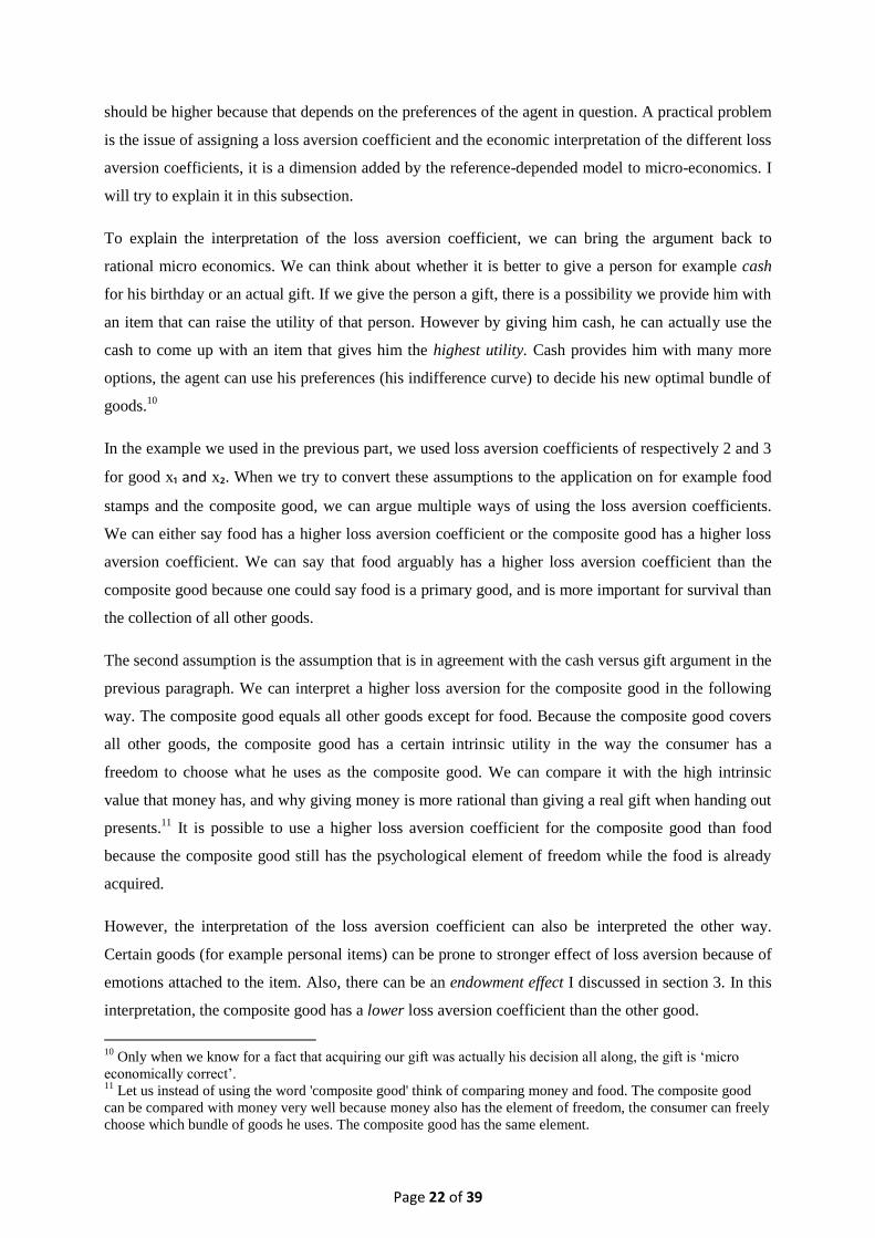
Figure 9

Kahneman en Tversky show in their 1991 paper a practical application which I illustrated in figure 9.

The fact point X and Y both lie on the indifference curve means in the SEM that the economic agent is

indifferent between either allocations. However, let us look at it from a prospect theory (loss averse)

point of view.

Kahneman and Tversky (1991) mention that the situation R1 (high leisure time, low) income will

cause that person to prefer point X to point Y. Situation R2 (high income, low leisure time) will cause

the person to prefer point Y to X.

This obviously violates the essential property of an indifference curves, which states that all points on

the curve yield equal utility and is caused by the loss aversion opportunity effect I introduced last

section. Traveling from R2 to point Y means two gains but traveling from R2 to X means a loss in

income. Because income is high, the potential loss is the entire area below point R2 and has a bigger

impact on utility than the bigger gain in leisure. The same thing also holds for R1. From R1 to X

means a gain in leisure and a small gain in income, which is preferred to a move to Y because of the

small loss in leisure the latter one would induce.

Although the theory is in compliance with research on the endowment effect and prospect theory, it is

in violation with essential core principles of the SEM. It is the first problem I face when trying to

incorporate reference-dependency in the SEM. The principle of indifference is not satisfied.

Income

Leisure

SEM Indifference curve with reference points

U (alpha) U (beta) R1 R2

Y

R2

R1 X

R2

R1

of 39

In this part I showed the practical differences I found when dealing with practical situations in either

the SEM and the reference-depended model. The loss aversion coefficients brings a new dimension to

the first step of micro economic analysis. The new best affordable bundle at the R-D model is always

at the reference point because the reference point13

is the focal point when dealing with losses and

gains while at the SEM, the income and substitution effect drive the agent to having a new best bundle

that has a different ratio than before.

13

When we let the indifference curve adjust to the new reference points (as shown in section 4.3).

of 39

5. Experiment

In this part of the thesis I want to include experiments that can test if there is any truth to the reference-

dependency and loss aversion this thesis is about. I want this experiment to be used to answer

questions like: "Is it correct to really put so much value on the reference point as the R-D model does",

or "is the diminishing marginal utility an overrated concept?".

The core of the experiment is having multiple treatment groups and finding out whether the position of

the treatments groups reference point actually influences the amount of time worked. The first

experiment takes an hour and consists of a dull work assignment, and when the (isolated) individual

quits this assignment he gets to watch a funny comedy (leisure). In the hypothetical experiment, we

can actually think of 3 possible reference points.

A. 10 minutes of unpaid work (and then an amount of work chosen by the individual against a

small wage).

B. 10 minutes of unpaid work and a bonus fixed wage of 10 euro (and then an amount of work

chosen by the individual against a small wage).

C. Just an amount of work chosen by the individual against a small wage, and no 10 euro bonus

wage.

Plan A has a reference point with a small amount of (variable) income and an also a small amount of

leisure time. Plan B has a higher income reference point and the same small leisure reference point as

point A. Plan C has the small amount of income reference point (same as point A) but a higher leisure

reference point. We can introduce another treatment group which reference points do not include the

10 minutes of unpaid work.

The predictions from section 4 suggest that when we use the R-D model, the reference point can make

people work the same amount in plan A and B because the reference points adjusts, and the amount of

leisure in both reference points is the same here. In the SEM, there will be an income effect, a

substitution effect and diminishing marginal utility influencing the optimal choice and here, both plans

will probably have different optimal amounts of leisure (the exact predictions are again determined by

personal preferences of the individual in question).

Another experiment I also want to discuss is executed in the study Reference Points and Effort

Provision by (Johannes Abeler, Armin Falk, Lorenz Goette, and David Huffman, 2011). The

experiment I describe here is similar to the experiment in this paper, although it is simplified and

altered to fit into this thesis.

I want the experiment to cover 2 hypothesis.

Hypothesis 1) There is loss aversion in comparison to a reference point. Losses to the reference point

are valued more heavily than gains to the reference point because people adjust their cumulative piece

wage earned to the fixed rate to not do themselves short.

of 39

Hypothesis 2) When we increase the fixed rate and piece rate (not exclusively with the same factor),

we see significant different results between treatment groups.

When the experiment satisfies the first hypothesis, we have reasons to believe that the reference-

dependant model applies. With the second hypothesis I want to test if we can find results that are in

agreement with diminishing marginal utility.

The experiment has two treatment groups, both treatment groups take part in an easy but dull

assignments (the experiment in the mentioned study has counting zero's in a group of numbers) where

they are paid per performed assignment. They can stop at any moment and when they are done, they

have 50% chance they get paid according to the amount of tasks performed and 50% chance to get a

fixed amount. The one treatment group get a fixed amount of 3 euro's and the other treatment group

get a fixed amount of 7 euro's. The researchers found a significant result that the amount of tasks

performed was different in both groups.

The workers were reference-depended and used the 50% possible fixed amount as a reference point. If

they worked less than the fixed amount, and got that reward, they felt they would do themselves short.

There was proof that the both groups worked until the fixed amount was reached and then stopped

working to minimize feelings of losses.

I want to slightly alter this experiment (compared to the experiment in the paper) to include more

treatment groups with higher fixed amounts. Now that is has been established that there is a significant

difference between a 3 euro fixed amount and 7 euro fixed amount. It would be very interesting to see

if we can split the participants up in more groups and have for example a higher wage rate and fixed

amount and see if diminishing marginal utility has any effect and which effect dominates.

The good thing about this experiment I think is that it can very successfully create a reference point

that we can measure. We can test not only if people are reference-depended and value their losses

more than their gains, but also in what way the behavior changes when the fixed reward and wage rate

changes to see if this experiment is prone to diminishing marginal utility.

of 39

6. Discussion

Because I experienced problems when trying to use the same basic SEM principles with the reference-

dependent model when using multiple reference points (for example problems with monotonicity,

indifference, transitivity and only 1 possible best affordable bundle), I could not merge the two

principles of diminishing marginal utility and reference-dependency. We can argue that it is very hard

to have an interaction between the SEM and the reference point models when we have multiple

reference points.

Also the R-D model discussed in this thesis has a very basic utility curve, there is no transformation of

the quantity of a good to a certain level of utility. I would very much like to see an R-D model that

also has elements of diminishing marginal utility. Future research could include R-D models and SEM

models far more detailed and more precise to actually predict exact levels of different quantities of

goods.

Because the R-D model in this thesis is so basic, we can also argue whether it is realistic to assume

that if someone has a reference point, the optimum bundle will always be at that reference point (when

the reference point is on the budget line as in section 4.4). The truth does not just lie with either the

SEM or the R-D model, it is a combination and future research (and experiments) could perhaps

exactly measure which model is more dominant.

In this thesis I could also not model an indifference curve that actually showed diminishing marginal

utility. If someone would be able to combine a Cobb-Douglas utility function with the R-D model, we

could see reference-dependency and diminishing marginal utility in one model and see diminishing

marginal utility and loss aversion both present. However, one would probably encounter the same

problems I encountered in section 4.5 (for example indifference curves of different reference points

intersecting each other).

Also, this thesis could have a more detailed experiment which included a step for step plan in getting

data to support either the SEM or the R-D model.

Finally, I regret not being able to include a more detailed specification of how the income effect and

substitution effect interact to get a new optimal bundle in the SEM. I could not model this in a graph,

because I could not emulate a curve with diminishing marginal utility. This is necessary for a future

paper to precisely predict how the SEM would get a new optimal bundle when a given wage change

occurs.

of 39

7. Conclusion

I started this thesis with huge ambitions and a wish to come up with a way to do predictions with the

standard economic model that would have an element of loss aversion implemented in it. In this thesis

I tried to answer the following research question:

"How do loss aversion and reference point theories change the first step of micro economic analysis

and how do these behavioral economic models differ from the standard economic model."

I learned that an essential element of a SEM indifference curve is the diminishing marginal utility and

that the SEM has very strict principles like monotonicity and transitivity. When rational decision

making is assumed, the SEM can predict the optimal bundle of consumption when the budget and

preferences of people are known.

Prospect theory shows that people do not always behave rationally and I discussed that people can be

loss averse. People would value their losses more negatively, as gains compared to a reference point,

even when the quantity gained and lost is exactly the same. I also explained the relevance of the

reference point in prospect theory.

The importance of the reference point really became clear when I used a reference-depended model to

draw indifference curve that were subject to a reference point. I used examples to explain what effect

a loss aversion coefficient could have in explaining the different intrinsic values between goods with

help of micro economic theory. When I used a change in endowment, with different reference points. I

encountered problems of transitivity and monotonicity in the situation when different reference points

were used. Problems that will make it very difficult to combine reference-dependency and SEM in the

future. Because different reference points are the cause of the huge differences between indifference

curves, my conclusion is that in a reference based model, a change of reference points can drastically

alter a person‟s preferences.

With the SEM, diminishing marginal utility, the income and substitution effect can change the position

of the indifference curve, for example to intersect a new budget curve (at one new point). The R-D

model however is completely depended on how the reference point behaves and if the reference points

shift, entire new preferences are formed and if the reference point is on the budget line, that will

always be the best possible bundle. In part 4.4 I showed the different practical consequences that

caused. I used an example where in the R-D model there was a wage change, and the individual would

not change his amount of hours worked because his reference point would adjust, a situation that

would not occur in the SEM. When we assess a situation with the SEM, and we take into account the

R-D model, we have to think about how the agents reference point adjusts to the changes and how the

losses and gains of utility interact differently on total utility.

of 39

I conclude that reference-dependency (especially when the reference points shift) cause monotonicity

and transitivity problems in a SEM model, which make it very difficult to implement loss aversion

into the SEM. However for future research I think it would be very interesting and valuable if one

could graphically show the results when a Cobb-Douglas utility function is used with a reference-

depended model. In part 5 of this thesis I also included ideas for experiments to test whether we see

reference-dependency in it subjects, to see if the subjects are prone to diminishing marginal utility and

see which effect dominates the results.

In the appendix will be a short description of calculations and the used graphs.

of 39

Appendix

I will use this appendix to elaborate my calculations and how I derived the graphs.

Figure 1 & 9: the Cobb-Douglas shaped indifference curves with continuous convex shape.

I derived these curves using a x1 range from (0,..10) and x2 from (0,..10) and using

u(x1)= I multiplied all values by -1 and all values +9 to get a positive utility.

I graphed x1 for the x-data and x2 for the y-data.

Figure 2, 4, 5, 6, 7, 8:

These indifference curves are drawn with the reference-depended model as covered in section 4.1

I only used loss aversion coefficients for x1 and x2 of respectively 2 and 3. I would chose a total

utility for example -10, 0, 10 or 20, if I would chose a utility of 0, I would solve this function.

x x x this wou d get the point x on the indiffe ence cu ve

when R(x1) and R(x2) are given.

An R(x1) of 20 and R(x2) of 30 would get an x1 of 0 and a x2 of 70. The next point to find would be

x1 of 10 and a x2 that follows out of that equitation.

I would only use this form when x1 < R(x1) and x2>R(x2) when x2 passes the reference point and we

experience a loss in x1, the function to solve would change to:

x x x this wou d get the point x when the reference point is

again, (20,30) and x1 is 30, we get the point x2 is

. This form would be used when x2<R(x2) and

x1>R(x1)

When there was a loss in both x1 and x2 I would use the following equation to derive the quantities for

a total utility of say -10, with loss aversion coefficients in both term for x1<R(x1) and x2<R(x2):

x x x

of 39

References

Books

Bowles S. - "Microeconomics, Behavior, Institutions, and Evolution (2006)(ISBN 0691126380)

Frank R. - "Microeconomics and Behavior" (2002)( ISBN 0072483342)

Gerrard B. (ed.) - "The Economics of rationality" (1993)(ISBN 0415068754)

Pinker S, -"How the mind works" (1999) (ISBN 0393318486)

Rubinstein A.- " Lecture Notes in Microeconomic Theory" (2006)(ISBN 0691120315)

Wilkinson N. - "An Introduction To Behavioral Economics" (2008) (ISBN 0230532594)

Papers

Abeler, Johannes; Falk, Armin; Goette, Lorenz; Huffman, David - “Reference Points and Effort

Provision,” (American Economic Review 101, 470–492.) (2011)

Allen R. G. D. -"The Nature of Indifference Curves", (The Review of Economic Studies, Vol. 1, No. 2,

pp. 110-121) (Feb., 1934)

Benartzi, Shlomo and Richard Thaler, "Myopic Loss Aversion and the Equity Premium Puzzle",

(Quarterly Journal of Economics 110, 1995, 73-92.)

Camerer, Colin F. - "Prospect theory in the wild: Evidence from the field", (1998), (California Institute

of Technology).

Hanemann, W. Michael.- "Willingness to Pay and Willingness to Accept: How Much Can They

Differ?" (American Economic Review, June 1991, 81(3), pp. 635-47)

Huang, J-J- "Revised behavioural models for riskless consumer choice", (Kainan University, Taoyuan,

Taiwan), (Journal of the Operational Research Society 60, 1237 --1243), (2009)

Kahneman, Daniel; Knetsch, Jack L. and Thaler, Richard H., "Anomalies: The Endowment Effect,

Loss Aversion, and Status Quo Bias" , (The Journal of Economic Perspectives Vol. 5, No. 1 (Winter,

1991), pp. 193-206)

Kahneman, Daniel; Tversky ,Amos, "Prospect Theory: An Analysis of Decision under Risk",

(Econometrica, Vol. 47, No. 2. (Mar., 1979), pp. 263-292.)

of 39

Kahneman, D., Knetsch, J., & Thaler, R. (1990). "Experimental Test of the endowment effect and the

Coase Theorem." (Journal of Political Economy 98(6), 1325-1348.)

Mehra, Rajneesh and Prescott, Edward- "The equity premium puzzle".,(Journal of Monetary

Economics, 1985.)

Putler, Daniel S. - "Incorporating Reference Price Effects into a Theory of Consumer Choice",

(Marketing Science, Vol. 11, No. 3 (Summer, 1992), pp. 287-309)

Shefrin, Hersh and Statman, Meir- "The Disposition to Sell Winners Too Early and Ride Losers Too

Long: Theory and Evidence", (The Journal of Finance, Vol. 40, No. 3, Papers and Proceedings of the

Forty-Third Annual Meeting American Finance Association, Dallas, Texas, December 28-30, 1984

(Jul., 1985), pp. 777-790)

Thaler, Richard - "Towards a positive theory of consumer choice", (Cornefl University, ithaca, NY

14853, USA), (Journal of Economic Behavior and Organization l 3960) (1980)

Tversky, A. & Kahneman, D. -"Loss Aversion in Riskless Choice: A Reference Dependent Model." ,

(Quarterly Journal of Economics 106, 1039-1061. (1991))

Miscellaneous & Websites

Picture titelpage: http://empwaynek.files.wordpress.com/2011/05/loss-aversion.jpg?w=400

Figure 3, S shaped value function : FEB13061 Behavioral economics by dr. Baillon – slides „Lecture 1

– Risk and Prospect Theory_1‟, sheet 19. Alterations done myself.

http://en.wikipedia.org/wiki/Indifference_curves

http://en.wikipedia.org/wiki/Endowment_effect

http://en.wikipedia.org/wiki/Loss_aversion

http://empwaynek.files.wordpress.com/2011/05/loss-aversion.jpg?w=400

http://en.wikipedia.org/wiki/Indifference_curves

http://en.wikipedia.org/wiki/Endowment_effect

http://en.wikipedia.org/wiki/Loss_aversion

combining loss aversion with the standard economic model

Documents