combustion - cerfacscfdbib/repository/tr_cfd_04_122.pdf · more complex than those used in...
TRANSCRIPT

Combustion
T. J. Poinsot1 and D. P. Veynante2
1 Institut de Mecanique des Fluides de Toulouse31400 TOULOUSE, FRANCE
2 Laboratoire EM2C, Ecole Centrale de Paris92295 CHATENAY MALABRY, FRANCE
ABSTRACT
This chapter describes the basic phenomena controlling reacting flows and the correspondingcomputational methodologies. Combustion regimes (premixed or diffusion flames, laminar or turbulentcases, stable or unstable behavior) are first defined before introducing the basic terminology requiredto understand numerical techniques for reacting flows. The governing equations for combustion aremore complex than those used in classical aerodynamics and their specificities are discussed beforedescribing numerical methods for laminar flames. Finally, the various methods used for turbulentflames are discussed, focusing on recent techniques such as Direct Numerical Simulations and LargeEddy Simulations.
key words: Combustion; reacting flows
Contents
1 INTRODUCTION 2
2 COMBUSTION REGIMES 42.1 Premixed flames . . . . . . . . . . . . . . . . . . . . . . . . . . . . . . . . . . . 52.2 Non-premixed flames . . . . . . . . . . . . . . . . . . . . . . . . . . . . . . . . . 62.3 Partially premixed flames . . . . . . . . . . . . . . . . . . . . . . . . . . . . . . 72.4 Stable and unstable flames . . . . . . . . . . . . . . . . . . . . . . . . . . . . . . 7
2.4.1 Thermodiffusive instabilities . . . . . . . . . . . . . . . . . . . . . . . . . 72.4.2 Flame/acoustic interactions . . . . . . . . . . . . . . . . . . . . . . . . . 9
3 GOVERNING EQUATIONS 113.1 Balance equations . . . . . . . . . . . . . . . . . . . . . . . . . . . . . . . . . . 113.2 Viscous tensor . . . . . . . . . . . . . . . . . . . . . . . . . . . . . . . . . . . . 113.3 Transport terms . . . . . . . . . . . . . . . . . . . . . . . . . . . . . . . . . . . 12
3.3.1 Molecular transport . . . . . . . . . . . . . . . . . . . . . . . . . . . . . 123.3.2 Usual simplified approximations . . . . . . . . . . . . . . . . . . . . . . 13
3.4 Thermochemical data and state equation . . . . . . . . . . . . . . . . . . . . . 133.5 Reaction terms and kinetics . . . . . . . . . . . . . . . . . . . . . . . . . . . . . 14
Encyclopedia of Computational Mechanics. Edited by Erwin Stein, Rene de Borst and Thomas J.R. Hughes.c© 2004 John Wiley & Sons, Ltd.

2 ENCYCLOPEDIA OF COMPUTATIONAL MECHANICS
4 COMBUSTION TERMINOLOGY AND BASICS 15
4.1 Overall reaction and stoichiometry . . . . . . . . . . . . . . . . . . . . . . . . . 15
4.2 Mixture fraction . . . . . . . . . . . . . . . . . . . . . . . . . . . . . . . . . . . 16
4.2.1 Definitions . . . . . . . . . . . . . . . . . . . . . . . . . . . . . . . . . . 16
4.2.2 Pure mixing . . . . . . . . . . . . . . . . . . . . . . . . . . . . . . . . . . 17
4.2.3 Single step chemical reaction . . . . . . . . . . . . . . . . . . . . . . . . 18
4.2.4 Extensions . . . . . . . . . . . . . . . . . . . . . . . . . . . . . . . . . . 19
4.3 Progress variable . . . . . . . . . . . . . . . . . . . . . . . . . . . . . . . . . . . 20
4.4 Ignition times . . . . . . . . . . . . . . . . . . . . . . . . . . . . . . . . . . . . . 20
4.5 Flame speeds . . . . . . . . . . . . . . . . . . . . . . . . . . . . . . . . . . . . . 20
4.6 Flame stretch . . . . . . . . . . . . . . . . . . . . . . . . . . . . . . . . . . . . . 22
5 HOMOGENEOUS REACTORS AND LAMINAR FLAMES 23
5.1 Zero-dimensional tools . . . . . . . . . . . . . . . . . . . . . . . . . . . . . . . . 23
5.1.1 Ignition times computation . . . . . . . . . . . . . . . . . . . . . . . . . 23
5.1.2 Perfectly stirred reactors . . . . . . . . . . . . . . . . . . . . . . . . . . . 24
5.2 Steady one-dimensional tools . . . . . . . . . . . . . . . . . . . . . . . . . . . . 24
5.3 Other laminar flames . . . . . . . . . . . . . . . . . . . . . . . . . . . . . . . . . 25
6 TURBULENT FLAMES 25
6.1 Introduction . . . . . . . . . . . . . . . . . . . . . . . . . . . . . . . . . . . . . . 25
6.2 Physical analysis - Combustion diagrams . . . . . . . . . . . . . . . . . . . . . . 29
6.3 Tools for combustion modeling . . . . . . . . . . . . . . . . . . . . . . . . . . . 32
6.3.1 Introduction . . . . . . . . . . . . . . . . . . . . . . . . . . . . . . . . . 32
6.3.2 Geometrical approach . . . . . . . . . . . . . . . . . . . . . . . . . . . . 32
6.3.3 Statistical approach . . . . . . . . . . . . . . . . . . . . . . . . . . . . . 34
6.3.4 Mixing approach . . . . . . . . . . . . . . . . . . . . . . . . . . . . . . . 35
6.4 Bray-Moss-Libby analysis . . . . . . . . . . . . . . . . . . . . . . . . . . . . . . 35
1. INTRODUCTION
Burning fossil fuels produces more than two thirds of our energy production today and probablystill will in a century. Combustion is encountered in many practical systems such as boilers,heaters, domestic and industrial furnaces, thermal power plants, waste incinerators, automotiveand aeronautic engines, rocket engines,. . . The growing expectations on increasing efficiencyand reducing fuel consumption and pollutant emissions make the design of combustion systemsmuch more complex and the science of combustion a rapidly expanding field. Considering thecomplexity of the phenomena involved in flames and the difficulty and the costs of performingexperiments, numerical combustion is now gathering a large part of the research efforts.
In most applications, combustion occurs in gaseous flows and is characterized by:
• a strong and irreversible heat release. Heat is released in very thin fronts (typicalflame thicknesses are usually less than 0.5 mm) inducing strong temperature gradients(temperature ratios between burnt and fresh gases are of the order of 5 to 7).
Encyclopedia of Computational Mechanics. Edited by Erwin Stein, Rene de Borst and Thomas J.R. Hughes.
c© 2004 John Wiley & Sons, Ltd.
COMBUSTION 3
• highly nonlinear reaction rates ω. These rates follow Arrhenius laws: ω ∝∏N
k=1Yk exp(−Ta/T ) where the Yk are the mass fractions of the N species involved
in the reaction and Ta is an activation temperature. Ta is generally large so that reactionrates are extremely sensitive to temperature.
Combustion strongly modifies the flow field. In simple one-dimensional flames, burnt gases areaccelerated because of thermal expansion but more complex phenomena occur in turbulentflows: depending on the situation, turbulence may be either reduced or enhanced by flames.All these characteristics lead to serious numerical difficulties: simulations must handle stiffgradients in temperature, species mass fractions and, accordingly, in velocity fields. Note alsothat flow and chemical time and length scales, as well as species mass fractions may differ byseveral orders of magnitude. Fuel oxidation is generally fast compared to flow time scales butpollutant formation (nitric oxides, soot) may be quite slower. Major species (fuel, oxidizer,water, carbon dioxide) mass fractions are fractions of unity whereas pollutant mass fractionsare often measured in part per billion.
Various coupling mechanisms occur in combusting flow fields. Chemical reaction schemeshave to describe the fuel consumption rate, the formation of combustion products and pollutantspecies and should handle ignition, flame stabilization and quenching (full chemical schemesfor usual hydrocarbon fuels involve hundreds of species and thousands of reactions). Masstransfers of chemical species by molecular diffusion, convection and turbulent transportare also an important ingredient. The heat released by chemical reactions induces strongconductive, convective or radiative heat transfer inside the flow and with the surroundingwalls. Gaseous combustion also requires the description of the flow field (fluid mechanics). Fortwo (liquid fuel) and three (solid fuel) phase reacting systems, some other aspects must also beinvolved: spray formation, vaporization, droplet combustion,. . . Even for gaseous combustion,multiphase treatments may be needed: for example, soot particles (which can be formed inall flames) are carbon elements of large size transported by the flow motions. Some of thesephenomena are illustrated in Fig. 1 in the simple configuration, but very complex case, of acandle.
Because of the complexity of combustion and related phenomena, chemical reactions andfluid flow cannot be solved at the same time using brute force techniques, except in a fewacademic cases. Modeling and physical insight are required to build computational tools forreacting flows. The variety of approaches for numerical combustion indicates that there isno consensus today on the best path to follow. This is especially true for turbulent flameswhich represent most practical industrial applications. Therefore, the computation expert incombustion must have a deep knowledge of combustion theory and models. The objective of thischapter is to present the minimum elements required for this task and insist on recent advances.It does not attempt to replace classical textbooks on chemistry kinetics (Gardiner, 2000),multicomponent transport (Giovangigli, 1999), reacting flows (Glassman, 1977; Williams, 1985;Kuo, 1986; Turns, 1996; Peters, 2000) or numerical combustion (Oran and Boris, 1987; Poinsotand Veynante, 2001) but focusses on gathering the essential notions needed for computations.
The presentation is organized as follows: first, a description of the different regimes found inflames is given (Section 2). Each of these regimes usually requires different computationalapproaches. Section 3 discusses the equations solved for reacting flows and presents thedifferences between these equations and those used for classical aerodynamics. The basicterminology needed to understand the computational methods in combustion is provided in
Encyclopedia of Computational Mechanics. Edited by Erwin Stein, Rene de Borst and Thomas J.R. Hughes.
c© 2004 John Wiley & Sons, Ltd.

4 ENCYCLOPEDIA OF COMPUTATIONAL MECHANICS
Air entrainment(natural convection)
Solid stearin
Sootradiation
Fueloxidation
Liquid fuel
Burnt gases(natural convection)
Gaseous fuel
Light(radiative heat tranfer)
Figure 1. A very difficult flame: the candle. The solid stearin fuel is first heated by heat transferinduced by combustion. The liquid fuel reaches the flame by capillarity along the wick and is vaporized.Fuel oxidation occurs in thin blue layers (the color corresponds to the spontaneous emission of theCH radical). Unburnt carbon particles are formed because the fuel is in excess in the reaction zone.Corresponding to an imperfect combustion, this soot is welcomed in the case of the candle because it isthe source of the yellow light emission. Flow (entrainment of heavy cold fresh air and evacuation of hotlight burnt gases) is induced by natural convection (a candle cannot burn in zero-gravity environment).
Straight arrows correspond to mass transfer and broken arrows denote heat transfer.
Section 4. The last sections present applications to laminar (Section 5) and turbulent flames(Section 6). The whole presentation is limited to gaseous combustion and does not addressmultiphase reacting flows.
2. COMBUSTION REGIMES
To describe the various possible states observed in reacting flows it is useful to introduce aclassification based on combustion regimes. To first order flames can be (see Table I):
(a) premixed, non-premixed or partially premixed (Sections 2.1 to 2.3),
(b) laminar or turbulent,
(c) stable or unstable (Section 2.4).
Criterion (a) depends on the way retained to introduce the reactants into the combustionzone and is one of the main parameters controlling the flame regime. Fuel and oxidizer maybe mixed before the reaction takes place (premixed flames, Fig. 2a) or enter the reaction zoneseparately (non-premixed or diffusion flames, Fig. 2b).
Criterion (b) corresponds to the usual definition of turbulent states in which largeReynolds numbers lead to unsteady flows. Most practical flames correspond to turbulent flows:turbulence enhances combustion intensity and allows the design of smaller burners. It alsoincreases the modeling difficulties by orders of magnitude.
Encyclopedia of Computational Mechanics. Edited by Erwin Stein, Rene de Borst and Thomas J.R. Hughes.
c© 2004 John Wiley & Sons, Ltd.

COMBUSTION 5
Stream 1 (with fuel) Total flow rate: m1
Stream 2 (with oxidizer)Total flow rate: m2
Plenum or Long duct(mixing)
Flame
A
(a) mixing device and premixed flame (b) non-premixed (diffusion) flame
Flame
Stream 1 (with fuel) Total flow rate: m1
Stream 2 (with oxidizer)Total flow rate: m2
Figure 2. Classification of the combustion regime as a function of the reactant introduction scheme.
Flow / Flame premixed non-premixed
Laminar Bunsen burner LighterDomestic cooker Candle
Turbulent Gas turbines Industrial furnacesSpark ignited Otto engines Diesel engines, rockets
Table I. Some examples of practical applications in terms of premixed/non-premixed flame andlaminar/turbulent flow field.
Criterion (c) is more specific of reacting flows: in some situations, a flame may exhibit strongunsteady periodic motions (combustion instabilities) due to a coupling between acoustics,hydrodynamics and heat release.
Examples of flames corresponding to various types of criteria are described in the nextsections.
2.1. Premixed flames
In premixed combustion, the reactants, fuel and oxidizer, are assumed to be perfectly mixedbefore entering the reaction zone (Fig. 2a). Premixed flames propagate towards the fresh gasesby diffusion/reaction mechanisms: the heat released by the reaction preheats the reactants bydiffusion until reaction starts (reaction rates increase exponentially with temperature). A one-dimensional laminar premixed flame propagates relatively to the fresh gases at the so-calledlaminar flame speed sl (see discussion about flame speeds in section 4.5), depending on thereactants, the fresh gases temperature and the pressure (Fig. 3). For usual fuels, the laminarflame speed is about 0.1 to 1 m/s.
When fresh gases are turbulent, the premixed flame propagates faster. Its speed sT iscalled the turbulent flame speed and is larger than the laminar flame speed (sT � sl). Theturbulent flame brush is also thicker than the laminar flame. From phenomenological arguments(Damkholer, 1940), experimental data (Abdel-Gayed et al., 1984; Abdel-Gayed and Bradley,1989) or theoretical analysis (Yakhot et al., 1992), many simple relations have been proposed
Encyclopedia of Computational Mechanics. Edited by Erwin Stein, Rene de Borst and Thomas J.R. Hughes.
c© 2004 John Wiley & Sons, Ltd.

6 ENCYCLOPEDIA OF COMPUTATIONAL MECHANICS
Fresh gases(Fuel + oxidizer) Burnt gases
Fuel mass fraction
Oxidizer mass fractionTemperature
Reaction rate
sl
reaction zonepreheat zone
Figure 3. Structure of a one-dimensional premixed laminar flame. For typical flames, the flamethickness, including preheat zone, is about 0.1 to 1 mm whereas the reaction zone itself is ten times
thinner. In this figure, the oxidizer is assumed to be in excess.
to link the turbulent flame speed sT to the laminar flame speed sl and the turbulence intensityof the incoming flow u′:
sT
sl
= 1 + α
(u′
sl
)n
(1)
where α and n are two model parameters of the order of unity. Unfortunately, sT is nota well defined quantity (Gouldin, 1996) and depends on various parameters (chemistrycharacteristics, flow geometry). Eq. (1) is consistent with the experimental observation that theturbulent flame speed increases with the turbulence intensity (at least up to the observationof a small decrease, the so-called “bending effect” just before flame extinction). In practice,however, relations similar to Eq. (1) exhibit rather poor agreement with data, when parametersare changed over a wide range of equivalence ratios and turbulence intensity (Duclos, Veynanteand Poinsot, 1993), suggesting that the concept of a unique turbulent flame speed is not correct.
Premixed flames offer high burning efficiency as the reactants are already mixed beforecombustion. The burnt gases temperature, which plays an important role in pollutantformation, can be easily controlled by the amount of fuel injected in the fresh gases. Butthese flames may be difficult to design because reactants should be mixed in well definedproportions (fuel/oxidizer mixtures burn only for a limited range of fuel mass fraction). Apremixed flame may also develop as soon as the reactants are mixed, leading to possible safetyproblems.
2.2. Non-premixed flames
In non-premixed flames (also called diffusion flames), reactants are introduced separately inthe reaction zone. The prototype of this situation is the fuel jet decharging in atmospheric air(Fig. 5). This configuration is very simple to design and to build: no pre-mixing is needed andit is safer: the flame cannot propagate towards the fuel stream because it contains no oxidizerand vice versa. Nevertheless, diffusion flames are less efficient because fuel and oxidizer mustmix by molecular diffusion before burning. The maximum burnt gases temperature is given by
Encyclopedia of Computational Mechanics. Edited by Erwin Stein, Rene de Borst and Thomas J.R. Hughes.
c© 2004 John Wiley & Sons, Ltd.

COMBUSTION 7
Pure oxidizer Pure fuel
Fuel mass fractionOxidizer mass fraction
Temperature
Reaction rate
Figure 4. Structure of a one-dimensional non-premixed laminar flame. Here fuel and oxidizer streamsare assumed to have the same temperature.
the temperature of fuel and oxidizer burning in stoichiometric proportions (the flame lies inthe region where fuel and oxidizer are in stoichiometric proportions, see Fig. 11) and cannot becontrolled easily. The structure of a one-dimensional non-premixed laminar flame is sketchedin Fig. 4.
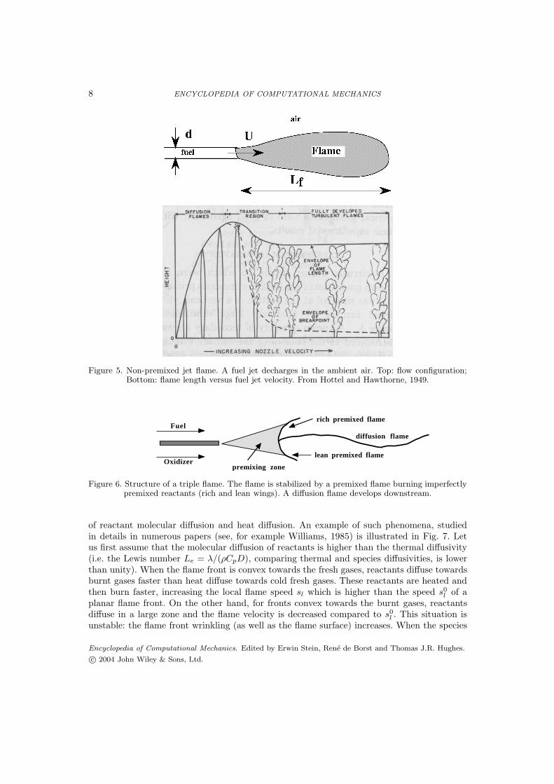
Turbulence is also found to enhance combustion processes in non-premixed flames asevidenced by Hottel and Hawthorne (1949) who measured the length of a diffusion flameburning a fuel jet decharging in ambient air as a function of the fuel flow rate (Fig. 5). Theflame length increases linearly with the fuel flow rate as long as the flow remains laminar.When the jet becomes turbulent, the flame length remains constant even when the flow rateincreases, showing an increase of the combustion intensity. Very large flow rates will lead tolifted flames (the flame is no more anchored to the jet exit) and then to blow-off or flamequenching.
2.3. Partially premixed flames
The previously described premixed and non-premixed flame regimes correspond to idealizedsituations. In practical applications, fuel and oxidizer cannot be perfectly premixed. Insome situations, an imperfect premixing is produced on purpose to reduce fuel consumptionor pollutant emissions. For example, in spark-ignited stratified charge internal combustionengines, the fuel injection is tuned to produce a quasi-stoichiometric mixture in the vicinity ofthe spark to promote ignition but a lean mixture in the rest of the cylinder. In non-premixedflames, fuel and oxidizer must meet to burn and ensure flame stabilization, leading to partiallypremixed zones. A prototype of this situation is the so-called triple flame where a partialpremixing of reactants occurs before the flame (Dold, 1989; Kioni et al., 1993; Domingo andVervisch, 1996; Muniz and Mungal, 1997; Kioni et al., 1998; Ghosal and Vervisch, 2000).A small premixed flame develops and stabilizes a diffusion flame as shown in Fig. 6. As aconsequence, partially premixed flames have now become topics of growing interest.
2.4. Stable and unstable flames
2.4.1. Thermodiffusive instabilitiesLaminar premixed flames exhibit intrinsic instabilities depending on the relative importance
Encyclopedia of Computational Mechanics. Edited by Erwin Stein, Rene de Borst and Thomas J.R. Hughes.
c© 2004 John Wiley & Sons, Ltd.
8 ENCYCLOPEDIA OF COMPUTATIONAL MECHANICS
Figure 5. Non-premixed jet flame. A fuel jet decharges in the ambient air. Top: flow configuration;Bottom: flame length versus fuel jet velocity. From Hottel and Hawthorne, 1949.
Fuel
Oxidizerpremixing zone
diffusion flame
rich premixed flame
lean premixed flame
Figure 6. Structure of a triple flame. The flame is stabilized by a premixed flame burning imperfectlypremixed reactants (rich and lean wings). A diffusion flame develops downstream.
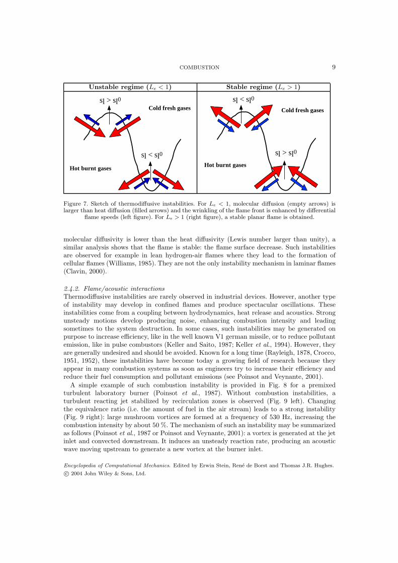
of reactant molecular diffusion and heat diffusion. An example of such phenomena, studiedin details in numerous papers (see, for example Williams, 1985) is illustrated in Fig. 7. Letus first assume that the molecular diffusion of reactants is higher than the thermal diffusivity(i.e. the Lewis number Le = λ/(ρCpD), comparing thermal and species diffusivities, is lowerthan unity). When the flame front is convex towards the fresh gases, reactants diffuse towardsburnt gases faster than heat diffuse towards cold fresh gases. These reactants are heated andthen burn faster, increasing the local flame speed sl which is higher than the speed s0
l of aplanar flame front. On the other hand, for fronts convex towards the burnt gases, reactantsdiffuse in a large zone and the flame velocity is decreased compared to s0
l . This situation isunstable: the flame front wrinkling (as well as the flame surface) increases. When the species
Encyclopedia of Computational Mechanics. Edited by Erwin Stein, Rene de Borst and Thomas J.R. Hughes.
c© 2004 John Wiley & Sons, Ltd.
COMBUSTION 9
Unstable regime (Le < 1) Stable regime (Le > 1)
Hot burnt gases
Cold fresh gases
sl < sl0
sl > sl0
Hot burnt gases
Cold fresh gases
sl < sl0
sl > sl0
Figure 7. Sketch of thermodiffusive instabilities. For Le < 1, molecular diffusion (empty arrows) islarger than heat diffusion (filled arrows) and the wrinkling of the flame front is enhanced by differential
flame speeds (left figure). For Le > 1 (right figure), a stable planar flame is obtained.
molecular diffusivity is lower than the heat diffusivity (Lewis number larger than unity), asimilar analysis shows that the flame is stable: the flame surface decrease. Such instabilitiesare observed for example in lean hydrogen-air flames where they lead to the formation ofcellular flames (Williams, 1985). They are not the only instability mechanism in laminar flames(Clavin, 2000).
2.4.2. Flame/acoustic interactionsThermodiffusive instabilities are rarely observed in industrial devices. However, another typeof instability may develop in confined flames and produce spectacular oscillations. Theseinstabilities come from a coupling between hydrodynamics, heat release and acoustics. Strongunsteady motions develop producing noise, enhancing combustion intensity and leadingsometimes to the system destruction. In some cases, such instabilities may be generated onpurpose to increase efficiency, like in the well known V1 german missile, or to reduce pollutantemission, like in pulse combustors (Keller and Saito, 1987; Keller et al., 1994). However, theyare generally undesired and should be avoided. Known for a long time (Rayleigh, 1878, Crocco,1951, 1952), these instabilities have become today a growing field of research because theyappear in many combustion systems as soon as engineers try to increase their efficiency andreduce their fuel consumption and pollutant emissions (see Poinsot and Veynante, 2001).
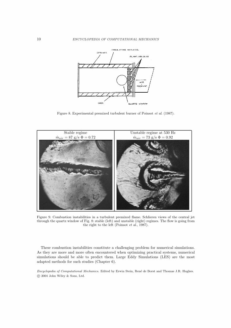
A simple example of such combustion instability is provided in Fig. 8 for a premixedturbulent laboratory burner (Poinsot et al., 1987). Without combustion instabilities, aturbulent reacting jet stabilized by recirculation zones is observed (Fig. 9 left). Changingthe equivalence ratio (i.e. the amount of fuel in the air stream) leads to a strong instability(Fig. 9 right): large mushroom vortices are formed at a frequency of 530 Hz, increasing thecombustion intensity by about 50 %. The mechanism of such an instability may be summarizedas follows (Poinsot et al., 1987 or Poinsot and Veynante, 2001): a vortex is generated at the jetinlet and convected downstream. It induces an unsteady reaction rate, producing an acousticwave moving upstream to generate a new vortex at the burner inlet.
Encyclopedia of Computational Mechanics. Edited by Erwin Stein, Rene de Borst and Thomas J.R. Hughes.
c© 2004 John Wiley & Sons, Ltd.
10 ENCYCLOPEDIA OF COMPUTATIONAL MECHANICS
Figure 8. Experimental premixed turbulent burner of Poinsot et al. (1987).
Stable regime Unstable regime at 530 Hzmair = 87 g/s Φ = 0.72 mair = 73 g/s Φ = 0.92
Figure 9. Combustion instabilities in a turbulent premixed flame. Schlieren views of the central jetthrough the quartz window of Fig. 8: stable (left) and unstable (right) regimes. The flow is going from
the right to the left (Poinsot et al., 1987).
These combustion instabilities constitute a challenging problem for numerical simulations.As they are more and more often encountered when optimizing practical systems, numericalsimulations should be able to predict them. Large Eddy Simulations (LES) are the mostadapted methods for such studies (Chapter 6).
Encyclopedia of Computational Mechanics. Edited by Erwin Stein, Rene de Borst and Thomas J.R. Hughes.
c© 2004 John Wiley & Sons, Ltd.
COMBUSTION 11
3. GOVERNING EQUATIONS
The equations controlling reacting flows differ from the usual conservation equations used forexample for aerodynamics in various aspects:
• since chemistry involves transforming species into other species, one additionalconservation equation must be written for each species of interest. Furthermore, in eachnew conservation equation, source terms must be added to describe the evolution ofspecies through chemical reactions,
• since the flow contains multiple species and large temperature differences,thermodynamical data, state equation and transport models must handle the fullequations required for a multispecies mixture.
3.1. Balance equations
For a reacting gas containing N species, the derivation of the conservation equations is acomplex task (Williams, 1985): a set of equations used in most practical cases is summarizedin Table II (Poinsot and Veynante, 2001) where ρ is the density, ui are the velocity components,Yk (for k = 1 to N) is the mass fraction of the kth species. The fk,i are the three components
of the volume forces fk acting on species k. Q is a volume source term for energy (radiationfor example). The species source terms due to chemical reactions ωk induce a heat release
term defined by ωT = −∑N
k=1∆ho
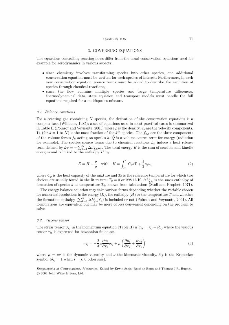
f,kωk. The total energy E is the sum of sensible and kineticenergies and is linked to the enthalpy H by:
E = H −p
ρwith H =
∫ T
T0
CpdT +1
2uiui (2)
where Cp is the heat capacity of the mixture and T0 is the reference temperature for which twochoices are usually found in the literature: T0 = 0 or 298.15 K. ∆ho
f,k is the mass enthalpy offormation of species k at temperature T0, known from tabulations (Stull and Prophet, 1971).
The energy balance equation may take various forms depending whether the variable chosenfor numerical resolutions is the energy (E), the enthalpy (H) or the temperature T and whether
the formation enthalpy (∑N
k=1∆ho
f,kYk) is included or not (Poinsot and Veynante, 2001). Allformulations are equivalent but may be more or less convenient depending on the problem tosolve.
3.2. Viscous tensor
The stress tensor σij in the momentum equation (Table II) is σij = τij −pδij where the viscoustensor τij is expressed for newtonian fluids as:
τij = −2
3µ
∂uk
∂xk
δij + µ
(∂ui
∂xj
+∂uj
∂xi
)(3)
where µ = ρν is the dynamic viscosity and ν the kinematic viscosity. δij is the Kroneckersymbol (δij = 1 when i = j, 0 otherwise).
Encyclopedia of Computational Mechanics. Edited by Erwin Stein, Rene de Borst and Thomas J.R. Hughes.
c© 2004 John Wiley & Sons, Ltd.

12 ENCYCLOPEDIA OF COMPUTATIONAL MECHANICS
Table II. A set of conservation equations for compressible reacting flows
Continuity: ∂ρ
∂t+ ∂ρui
∂xi= 0
Species (for k = 1 to N): ∂ρYk
∂t+ ∂
∂xi(ρ(ui + Vk,i)Yk) = ωk
Momentum: ∂∂t
ρui + ∂∂xj
ρuiuj = −
∂p
∂xi+
∂τij
∂xj+ ρ
PN
k=1Ykfk,i
Energy: ∂ρE
∂t+ ∂
∂xi(ρuiE) = ωT + ∂
∂xi(λ ∂T
∂xi) + Q
−
∂∂xi
(ρPN
k=1hs,kYkVk,i) + ∂
∂xj(σijui) + ρ
Pk Ykfk(u + Vk)
3.3. Transport terms
Transport description is a specific issue for reacting flows: the heat diffusivity λ, the kinematicviscosity ν and the molecular diffusion coefficients must be specified for multispecies gasesbefore solving Table II equations.
3.3.1. Molecular transport The molecular diffusion transport of the species k is described bythe three components Vk,i of the diffusion velocities Vk. The determination of the Vk’s requiresthe inversion of the diffusion matrix (Williams, 1985; Kuo, 1986; Bird, Stewart and Lightfoot,2002):
∇Xp =
N∑
k=1
XpXk
Dpk
(Vk − Vp) + (Yp − Xp)∇P
P+
ρ
p
N∑
k=1
YpYk(fp − fk) for p = 1, N (4)
where Dpk = Dkp is the binary mass diffusion coefficient of species p into species k and Xk isthe mole fraction of species k: Xk = YkW/Wk. The Soret effect (the diffusion of mass due totemperature gradients) is neglected in Eq. (4) (Williams, 1985).
Inverting Eq. (4) is a complex task which is often replaced by approximate solutions:recent studies (Ern and Giovangigli, 1994; Giovangigli, 1999) confirm, for example, that theHirschfelder-Curtiss approximate solution (Hirschfelder, Curtiss and Byrd, 1969) is the bestapproximation to the full solution of Eq. (4). This method replaces the resolution of Eq. (4)by a direct expression for the diffusion velocity Vk:
Vk = −1
Xk
Dk∇Xk (5)
where Dk is the diffusion coefficient of species k into the mixture. This method is widely usedand is probably the best choice in most codes. Note however that:
• Eq. (5) requires to add a correction velocity Vc to the convection velocity u to ensureglobal mass continuity.
• Eq. (5) is equivalent to the usual Fick’s law: Vk = −1/Yk(Dk∇Yk) only when pressure isconstant, volume forces negligible and the mixture contains only two species (Williams,1985). In other cases, Fick’s law should not be used.
Encyclopedia of Computational Mechanics. Edited by Erwin Stein, Rene de Borst and Thomas J.R. Hughes.
c© 2004 John Wiley & Sons, Ltd.
COMBUSTION 13
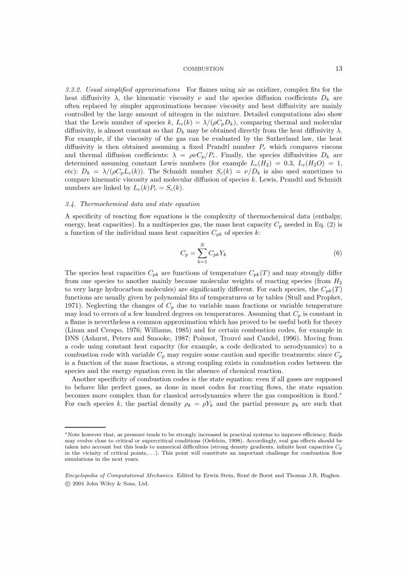
3.3.2. Usual simplified approximations For flames using air as oxidizer, complex fits for theheat diffusivity λ, the kinematic viscosity ν and the species diffusion coefficients Dk areoften replaced by simpler approximations because viscosity and heat diffusivity are mainlycontrolled by the large amount of nitrogen in the mixture. Detailed computations also showthat the Lewis number of species k, Le(k) = λ/(ρCpDk), comparing thermal and moleculardiffusivity, is almost constant so that Dk may be obtained directly from the heat diffusivity λ.For example, if the viscosity of the gas can be evaluated by the Sutherland law, the heatdiffusivity is then obtained assuming a fixed Prandtl number Pr which compares viscousand thermal diffusion coefficients: λ = ρνCp/Pr. Finally, the species diffusivities Dk aredetermined assuming constant Lewis numbers (for example Le(H2) = 0.3, Le(H2O) = 1,etc): Dk = λ/(ρCpLe(k)). The Schmidt number Sc(k) = ν/Dk is also used sometimes tocompare kinematic viscosity and molecular diffusion of species k. Lewis, Prandtl and Schmidtnumbers are linked by Le(k)Pr = Sc(k).
3.4. Thermochemical data and state equation
A specificity of reacting flow equations is the complexity of thermochemical data (enthalpy,energy, heat capacities). In a multispecies gas, the mass heat capacity Cp needed in Eq. (2) isa function of the individual mass heat capacities Cpk of species k:
Cp =
N∑
k=1
CpkYk (6)
The species heat capacities Cpk are functions of temperature Cpk(T ) and may strongly differfrom one species to another mainly because molecular weights of reacting species (from H2
to very large hydrocarbon molecules) are significantly different. For each species, the Cpk(T )functions are usually given by polynomial fits of temperatures or by tables (Stull and Prophet,1971). Neglecting the changes of Cp due to variable mass fractions or variable temperaturemay lead to errors of a few hundred degrees on temperatures. Assuming that Cp is constant ina flame is nevertheless a common approximation which has proved to be useful both for theory(Linan and Crespo, 1976; Williams, 1985) and for certain combustion codes, for example inDNS (Ashurst, Peters and Smooke, 1987; Poinsot, Trouve and Candel, 1996). Moving froma code using constant heat capacity (for example, a code dedicated to aerodynamics) to acombustion code with variable Cp may require some caution and specific treatments: since Cp
is a function of the mass fractions, a strong coupling exists in combustion codes between thespecies and the energy equation even in the absence of chemical reaction.
Another specificity of combustion codes is the state equation: even if all gases are supposedto behave like perfect gases, as done in most codes for reacting flows, the state equationbecomes more complex than for classical aerodynamics where the gas composition is fixed.∗
For each species k, the partial density ρk = ρYk and the partial pressure pk are such that
∗Note however that, as pressure tends to be strongly increased in practical systems to improve efficiency, fluidsmay evolve close to critical or supercritical conditions (Oefelein, 1998). Accordingly, real gas effects should betaken into account but this leads to numerical difficulties (strong density gradients, infinite heat capacities Cp
in the vicinity of critical points,. . . ). This point will constitute an important challenge for combustion flowsimulations in the next years.
Encyclopedia of Computational Mechanics. Edited by Erwin Stein, Rene de Borst and Thomas J.R. Hughes.
c© 2004 John Wiley & Sons, Ltd.

14 ENCYCLOPEDIA OF COMPUTATIONAL MECHANICS
pk = ρkRT/Wk where Wk is the molecular weight of species k. For the sum of all species
(k = 1 to N), the total pressure is p =∑N
k=1pk and the total density ρ =
∑Nk=1
ρk so that:
p =
N∑
k=1
pk =
(N∑
k=1
ρk
Wk
)RT =
ρRT
W(7)
where the molecular weight of the mixture is W =∑N
k=1(Yk/Wk)−1. In the state equation
p = ρRT/W , the molecular weight W changes when the composition changes. This additionalcomplexity has consequences for numerical techniques: for example, any error on one of thespecies balance equations will immediately impact the pressure field. Moreover, characteristicmethods used to specify boundary conditions in compressible codes using only one species(Poinsot and Lele, 1992) must be modified for combustion applications taking into accountmultiple species (Baum, Poinsot and Thevenin, 1994).
3.5. Reaction terms and kinetics
In typical combustion processes, hundreds of species react through hundreds or thousands ofchemical reactions. For each species k, a conservation equation is needed (see Table II) inwhich an expression is needed for the chemical source term ωk. A standard formalism is usedto formulate these terms in combustion. Consider N species reacting through M reactions:
N∑
k=1
ν′kjMk
N∑
k=1
ν′′
kjMk for j = 1, M (8)
where Mk is a symbol for species k, ν′kj and ν
′′
kj are the molar stoichiometric coefficients ofspecies k in reaction j. Mass conservation requires:
N∑
k=1
ν′kjWk =
N∑
k=1
ν′′
kjWk orN∑
k=1
νkjWk = 0 for j = 1, M (9)
where νkj = ν′′
kj − ν′kj . The mass rate ωk for species k is the sum of rates ωkj produced by all
M reactions:
ωk =
M∑
j=1
ωkj = Wk
M∑
j=1
νkjQj withωkj
Wkνkj
= Qj (10)
where Qj is the rate of progress of reaction j. This rate Qj involves a forward reaction (fromleft to right in Eq. 8) and a reverse reaction (right to left) and is written:
Qj = Kfj
N∏
k=1
(ρYk
Wk
)ν′
kj
− Krj
N∏
k=1
(ρYk
Wk
)ν′′
kj
(11)
The forward (Kfj) and reverse (Krj) reaction rates for reaction j are given by Arrhenius-typeexpressions:
Kfj = AfjTβj exp
(−
Ej
RT
)= AfjT
βj exp
(−
Taj
T
)(12)
For each forward or reverse reaction, three parameters must be specified: the preexponentialfactor Afj , the temperature exponent βj and the activation energy Ej (or the activation
Encyclopedia of Computational Mechanics. Edited by Erwin Stein, Rene de Borst and Thomas J.R. Hughes.
c© 2004 John Wiley & Sons, Ltd.

COMBUSTION 15
temperature Taj = Ej/R). For a typical hydrocarbon / air kinetic scheme involving up tothousand chemical reactions (M = 1000), 3000 parameters must be specified. Considering thedifficulty of determining these constants (Miller, 1996) but also the fact that some importantelementary reactions may be missing in the global scheme makes flame computations difficultand highly dependent on the quality (and the defaults) of the kinetic data.
4. COMBUSTION TERMINOLOGY AND BASICS
This section describes some basic combustion concepts required to understand the descriptionof numerical tools for reacting flows. First, the notions of stoichiometry (Section 4.1), mixturefraction (Section 4.2) and progress variable (Section 4.3) are defined. Section 4.4 introducesignition times while Section 4.5 present flame speeds definitions. Finally, Section 4.6 describesan essential parameter controlling the dynamics of flame fronts: stretch.
4.1. Overall reaction and stoichiometry
Consider ν′F moles of fuel reacting with ν′
O moles of oxidizer to give products:
ν′F F + ν′
OO → Products (13)
For example, CH4 + 2O2 → CO2 + 2H2O. In terms of mass, this equation is written:
F + s O → Products (14)
expressing that one kilogram of fuel reacts with s kilograms of oxidizer leading to (1 + s)kilograms of combustion products. The stoichiometric ratio s is defined by:
s =ν′
OWO
ν′F WF
(15)
where WF and WO are the molecular weights of fuel and oxidizer respectively.Fuel and oxidizer are in stoichiometric proportions in a gas mixture when their mass fractions
are such that:(YO/YF )st = s (16)
A given fuel / oxidizer mixture is characterized by its equivalence ratio Φ defined as:
Φ =YF /YO
(YF /YO)st
= sYF
YO
(17)
When the mixture is stoichiometric, Φ = 1. The mixture is called lean when Φ < 1 (oxidizeris in excess compared to fuel) and rich when Φ > 1 (fuel is in excess compared to oxidizer).
Premixed gases are usually created by mixing a fuel stream (total mass flow rate: m<1>,fuel mass fraction Y <1>
F ) with an oxidizer stream (total mass flow rate: m<2>, oxidizer massfraction Y <2>
O ). Stream 1 contains fuel and stream 2 contains the oxidizer (oxygen for example).Both streams can also contain other gases such as nitrogen: for fuel/air flames, for example,the oxidizer (oxygen) is diluted with nitrogen and Y <2>
O = 0.233. After a plenum or a longduct (Fig. 2a) the two streams are perfectly mixed. At the combustor inlet (point A), fuel andoxidizer mass fractions are given by:
Y AF = Y <1>
F
m<1>
m<1> + m<2>
and Y AO = Y <2>
O
m<2>
m<1> + m<2>
(18)
Encyclopedia of Computational Mechanics. Edited by Erwin Stein, Rene de Borst and Thomas J.R. Hughes.
c© 2004 John Wiley & Sons, Ltd.
16 ENCYCLOPEDIA OF COMPUTATIONAL MECHANICS
Stream 1:species Yk<1>
enthalpy h<1> z 1-z
Fresh mixture
h = z h<1> + (1-z) h<2>
Pure mixing Pure mixingYk= z Yk<1> + (1-z) Yk<2>
Stream 2:species Yk<2>
enthalpy h<2>
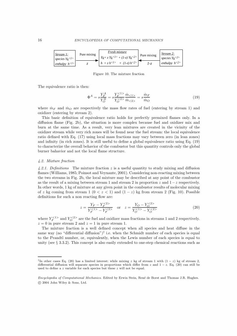
Figure 10. The mixture fraction
The equivalence ratio is then:
ΦA = sY A
F
Y BO
= sY <1>
F
Y <2>O
m<1>
m<2>
= smF
mO
(19)
where mF and mO are respectively the mass flow rates of fuel (entering by stream 1) andoxidizer (entering by stream 2).
This basic definition of equivalence ratio holds for perfectly premixed flames only. In adiffusion flame (Fig. 2b), the situation is more complex because fuel and oxidizer mix andburn at the same time. As a result, very lean mixtures are created in the vicinity of theoxidizer stream while very rich zones will be found near the fuel stream: the local equivalenceratio defined with Eq. (17) using local mass fractions may vary between zero (in lean zones)and infinity (in rich zones). It is still useful to define a global equivalence ratio using Eq. (19)to characterize the overall behavior of the combustor but this quantity controls only the globalburner bahavior and not the local flame structure.
4.2. Mixture fraction
4.2.1. Definitions The mixture fraction z is a useful quantity to study mixing and diffusionflames (Williams, 1985; Poinsot and Veynante, 2001). Considering non-reacting mixing betweenthe two streams in Fig. 2b, the local mixture may be described at any point of the combustoras the result of a mixing between stream 1 and stream 2 in proportion z and 1−z respectively.In other words, 1 kg of mixture at any given point in the combustor results of molecular mixingof z kg coming from stream 1 (0 < z < 1) and (1 − z) kg from stream 2 (Fig. 10). Possibledefinitions for such a non reacting flow are:
z =YF − Y <2>
F
Y <1>F − Y <2>
F
or z =YO − Y <2>
O
Y <1>O − Y <2>
O
(20)
where Y <1>F and Y <2>
O are the fuel and oxidizer mass fractions in streams 1 and 2 respectively.z = 0 in pure stream 2 and z = 1 in pure stream 1.
The mixture fraction is a well defined concept when all species and heat diffuse in thesame way (no “differential diffusion”)† i.e. when the Schmidt number of each species is equalto the Prandtl number, or, equivalently, when the Lewis number of each species is equal tounity (see § 3.3.2). This concept is also easily extended to one-step chemical reactions such as
†In other cases Eq. (20) has a limited interest: while mixing z kg of stream 1 with (1 − z) kg of stream 2,differential diffusion will separate species in proportions which differ from z and 1 − z. Eq. (20) can still beused to define a z variable for each species but these z will not be equal.
Encyclopedia of Computational Mechanics. Edited by Erwin Stein, Rene de Borst and Thomas J.R. Hughes.
c© 2004 John Wiley & Sons, Ltd.
COMBUSTION 17
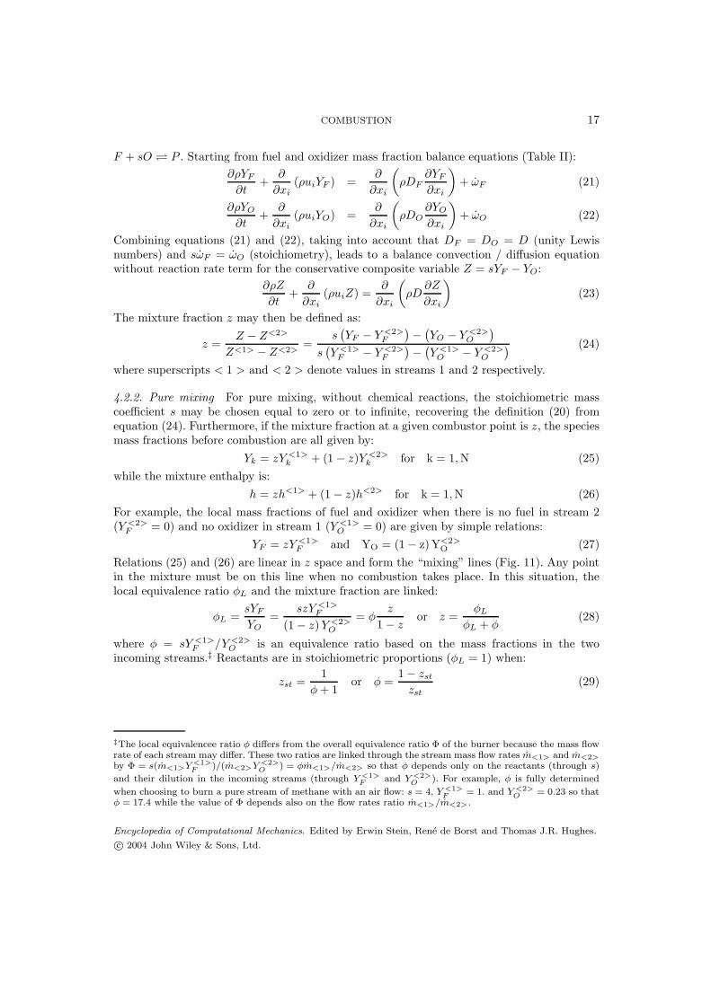
F + sO P . Starting from fuel and oxidizer mass fraction balance equations (Table II):
∂ρYF
∂t+
∂
∂xi
(ρuiYF ) =∂
∂xi
(ρDF
∂YF
∂xi
)+ ωF (21)
∂ρYO
∂t+
∂
∂xi
(ρuiYO) =∂
∂xi
(ρDO
∂YO
∂xi
)+ ωO (22)
Combining equations (21) and (22), taking into account that DF = DO = D (unity Lewisnumbers) and sωF = ωO (stoichiometry), leads to a balance convection / diffusion equationwithout reaction rate term for the conservative composite variable Z = sYF − YO:
∂ρZ
∂t+
∂
∂xi
(ρuiZ) =∂
∂xi
(ρD
∂Z
∂xi
)(23)
The mixture fraction z may then be defined as:
z =Z − Z<2>
Z<1> − Z<2>=
s(YF − Y <2>
F
)−(YO − Y <2>
O
)
s(Y <1>
F − Y <2>F
)−(Y <1>
O − Y <2>O
) (24)
where superscripts < 1 > and < 2 > denote values in streams 1 and 2 respectively.
4.2.2. Pure mixing For pure mixing, without chemical reactions, the stoichiometric masscoefficient s may be chosen equal to zero or to infinite, recovering the definition (20) fromequation (24). Furthermore, if the mixture fraction at a given combustor point is z, the speciesmass fractions before combustion are all given by:
Yk = zY <1>k + (1 − z)Y <2>
k for k = 1, N (25)
while the mixture enthalpy is:
h = zh<1> + (1 − z)h<2> for k = 1, N (26)
For example, the local mass fractions of fuel and oxidizer when there is no fuel in stream 2(Y <2>
F = 0) and no oxidizer in stream 1 (Y <1>O = 0) are given by simple relations:
YF = zY <1>F and YO = (1 − z)Y<2>
O (27)
Relations (25) and (26) are linear in z space and form the “mixing” lines (Fig. 11). Any pointin the mixture must be on this line when no combustion takes place. In this situation, thelocal equivalence ratio φL and the mixture fraction are linked:
φL =sYF
YO
=szY <1>
F
(1 − z)Y <2>O
= φz
1 − zor z =
φL
φL + φ(28)
where φ = sY <1>F /Y <2>
O is an equivalence ratio based on the mass fractions in the twoincoming streams.‡ Reactants are in stoichiometric proportions (φL = 1) when:
zst =1
φ + 1or φ =
1 − zst
zst
(29)
‡The local equivalencee ratio φ differs from the overall equivalence ratio Φ of the burner because the mass flowrate of each stream may differ. These two ratios are linked through the stream mass flow rates m<1> and m<2>
by Φ = s(m<1>Y <1>F )/(m<2>Y <2>
O ) = φm<1>/m<2> so that φ depends only on the reactants (through s)
and their dilution in the incoming streams (through Y <1>F and Y <2>
O ). For example, φ is fully determined
when choosing to burn a pure stream of methane with an air flow: s = 4, Y <1>F = 1. and Y <2>
O = 0.23 so thatφ = 17.4 while the value of Φ depends also on the flow rates ratio m<1>/m<2> .
Encyclopedia of Computational Mechanics. Edited by Erwin Stein, Rene de Borst and Thomas J.R. Hughes.
c© 2004 John Wiley & Sons, Ltd.
18 ENCYCLOPEDIA OF COMPUTATIONAL MECHANICS
where zst is the stoichiometric value of the mixture fraction z. Combining (28) and (29) gives:
φL =z(1 − zst)
zst(1 − z)(30)
Low values of the mixture fraction z (less than zst) correspond to lean mixtures (φL < 1) andvice versa.
Mixture fraction and equivalence ratio concepts both measure the quantity of fuel in themixture but are used for different purposes:
• The mixture fraction z (Eq. 24) varies linearly with the fuel mass fraction YF in themixture whereas the local equivalence ratio (Eq. 28) is an hyperbolic function of YF .
• In perfectly premixed unburnt reactants, the mixture fraction z is constant and is directlylinked to the equivalence ratio φL through Eq. (28).
• In burnt gases, the local equivalence ratio has no meaning since either the fuel or theoxidizer mass fraction is zero. The mixture fraction z, however, is conserved throughpremixed flame fronts and its value in the burnt gases can be used to evaluate theequivalence ratio of the fresh gases using Eq. (30). This property is often useful forsimulations of partially premixed flames.
4.2.3. Single step chemical reaction For a single step reaction, when there is no fuel in stream2 (Y <2>
F = 0) and no oxidizer in stream 1 (Y <1>O = 0), i.e. for a diffusion flame, equation (24)
may be recast as:
z =sYF − YO + Y <2>
O
sY <1>F + Y <2>
O
=φYF /Y <1>
F − YO/Y <2>O + 1
φ + 1(31)
After combustion has taken place, the resulting state can also be displayed in the z-diagram(Fig. 11). Assuming an irreversible infinitely fast chemical reaction (i.e. combustion proceedsfaster than all other flow phenomena), fuel and oxidizer cannot exist simultaneously and theflame is located where YF = YO = 0. Setting YF = YO = 0 in Eq. (31) gives the location ofthe flame front in mixture fraction space (Peters, 1984; Bilger, 1989):
z =Y <2>
O
sY <1>F + Y <2>
O
=1
φ + 1= zst (32)
The flame is infinitely thin and is located on the stoichiometric surface. The non-premixedflame structure in mixture fraction space is determined by the Burke-Schumann description:
YF = Y <1>F
z − zst
1 − zst
; YO = 0 for z ≥ zst
YF = 0 ; YO = Y <2>O
zst − z
zst
for z ≤ zst
(33)
This result may be extended to reversible infinitely fast reaction. In this situation, a chemicalequilibrium is reached where fuel and oxidizer may coexist. The flame still lies in the vicinityof the stoichiometric surface z = zst but its structure is determined by an equilibrium functionwhich is not necessarily straight lines in the z-diagram (Fig. 11).
Mixing and equilibrium lines constitute the basic tools in many models for diffusion orpartially premixed flames. While mixing lines are linear in z and can be constructed easily,
Encyclopedia of Computational Mechanics. Edited by Erwin Stein, Rene de Borst and Thomas J.R. Hughes.
c© 2004 John Wiley & Sons, Ltd.

COMBUSTION 19
Figure 11. Mixing and equilibrium lines in the z-diagram: shaded regions correspond to possible states.
equilibrium lines require more work: under certain assumptions (constant heat capacities,no dissociation of products), they can be obtained analytically (Williams, 1985; Poinsot andVeynante, 2001). In general, however, equilibrium codes such as Stanjan (available in thePREMIX package, Kee et al., 1985) are required (see Section 5.1). Generally, the equilibriumlines display an enthalpy (or temperature) maximum for z = zst: the maximum temperaturereached for a diffusion flame is obtained in near-stoichiometric regions. Such stoichiometricregions always exist in non-premixed flames so that these high temperature zones are difficultto avoid. Since these hot zones are responsible for the formation of pollutants such as NOx,the objective is often to minimize their size in modern combustion chambers. This can bedone by premixing fuel and oxidizer streams but may lead to other difficulties (safety, flameflash-back,. . . ).
4.2.4. Extensions The mixture fraction z has been introduced here for unity Lewis numbersand single-step reactions. These definitions may be extended to multi-step chemical reactionsif unity Lewis number is still assumed for all species. In this case, mixture fractions definitionsare based on the conservation of atomic elements (typically C, O or H). Each species containsfrom 1 to a maximum of P elementary elements. The mass fraction of the p-element is:
Zp =
N∑
k=1
akp
Wp
Wk
Yk = Wp
N∑
k=1
akp
Yk
Wk
(34)
where Wk is the atomic weight of species k and akp the number of elements of type p in speciesk: for example, if the species k is propane (C3H8) and if carbon (C) is the element p: akp = 3.The akp values do not depend on chemical reactions taking place between species. The mixture
Encyclopedia of Computational Mechanics. Edited by Erwin Stein, Rene de Borst and Thomas J.R. Hughes.
c© 2004 John Wiley & Sons, Ltd.
20 ENCYCLOPEDIA OF COMPUTATIONAL MECHANICS
fraction z is then defined as:
z =Zp − Z<2>
p
Z<1>p − Z<2>
p
(35)
where subscripts ¡1¿ and ¡2¿ denote Zp values in stream 1 and in stream 2 respectively. As allspecies diffuse in the same way (unity Lewis number), the value of the mixture fraction doesnot depend on the element p considered.
Extensions of the mixture fraction concept have been proposed when non-unity Lewisnumbers are encountered but are seldom used (Linan et al., 1994).
4.3. Progress variable
In premixed combustion, a progress variable Θ is usually introduced to quantify the reactionprogress using the temperature T or the fuel mass fraction YF :
Θ =T − T u
T b − T uor Θ =
YF − Y uF
Y bF − Y u
F
(36)
where superscripts u and b denote unburnt and burnt gas quantities respectively. The progressvariable is Θ = 0 in fresh gases and Θ = 1 in fully burnt ones. The use of the progress variableis especially interesting for a single step chemical reaction, for adiabatic conditions and withoutcompressibility effects assuming unity Lewis numbers : in this situation, species mass fractionsand temperature are closely related and definitions (36) are equivalent. Accordingly, only asingle balance equation for the progress variable is required to describe species and temperatureevolutions.
4.4. Ignition times
The time needed for the autoignition of a given mixture is an essential information in multiplecombustion problems such as rocket, piston engines, supersonic ramjets or safety problems(Glassman, 1977; Westbrook, 2000). Autoignition studies are usually formulated in terms ofinitial value problems: given an initial temperature and initial mass fractions, how long does ittake before strong energetic reactions start? This question may be studied theoretically usingsimplified assumptions but numerical approaches are often preferred because of the importanceof complex chemical kinetic and transport features in such phenomena (Section 5.1). As anexample, Fig. 12 presents a typical configuration where a low-temperature fuel (injected withstream 1) is mixed with a high-temperature oxidizer (stream 2). The mixture fraction z(Section 4.2) characterizes the resulting mixture. This mixture is then left to react and itsignition time tign is plotted as a function of z. The minimum ignition time (i.e. the fasterignition) is obtained for the most reactive value zmr of the mixture fraction z. When thetemperatures of both streams are identical, zmr ' zst: the ignition time is minimum whenreactants are mixed in stoichiometric proportions. When one of the streams has an highertemperature, the oxidizer in the example given in Fig. 12, zmr differs from the stoichiometricvalue zst of the mixture fraction and is shifted towards the higher temperature stream, herezmr < zst (Mastorakos, Baritaud and Poinsot, 1997).
4.5. Flame speeds
The intuitive notion of “flame speed”, describing the propagation of the flame front relativelyto the flow field, covers multiple combustion concepts used in models. First, only premixed or
Encyclopedia of Computational Mechanics. Edited by Erwin Stein, Rene de Borst and Thomas J.R. Hughes.
c© 2004 John Wiley & Sons, Ltd.

COMBUSTION 21
Stream 1:species Yk1
enthalpy h1 z 1-z
Fresh mixture
h = zh1 + (1-z)h2
Yk= Yk1 z + Yk1 (1-z)
Stream 2:species Yk2
enthalpy h2
Homogeneous mixing ignition code
z
tign
zmr zst No oxidizerNo fuel
Figure 12. Numerical determination of the ignition time of a given mixture.
partially premixed flames propagate and flame speeds concepts apply only to these situations.Second, two flame speeds are generally introduced (and sometimes confused) to describelaminar premixed flames (Table III).
Table III. Classification of laminar flame speeds.
Identification Notation Definition
Displacement sd Front speed relative to the flow
Consumption sc Speed at which reactants are consumed
The displacement speed corresponds to a purely kinematic definition in which the flamefront is described as an interface propagating at velocity sd relative to the flow: sd is thedifference between the absolute speed ~w of the flame in a fixed reference frame and the flowvelocity ~u in the same frame:
~w = ~u + sd~n or sd = (~w − ~u) · ~n (37)
where ~n is the unit vector normal to the flame front pointing towards the fresh gases. Theflame front displacement speed is commonly used in codes based on front tracking techniques(Section 6). Measuring sd may be a challenging task in many cases such as stagnation pointflames (Law, 1988; Egolfopoulos and Law, 1994) or curved flames (Dowdy, Smith and Taylor,1990; Aung, Hassan and Faeth, 1998; Poinsot, 1998) because the flow velocity ~u at the flamelocation is difficult to evaluate and varies rapidly along the flame normal.
The consumption velocity sc (Table III) measures the speed at which reactants are consumedand can be expressed as a function of the integral of the reaction rate along the normal ~n tothe flame front:
sc =1
ρ1
(Y u
F − Y bF
)+∞∫
−∞
ωF dn (38)
Encyclopedia of Computational Mechanics. Edited by Erwin Stein, Rene de Borst and Thomas J.R. Hughes.
c© 2004 John Wiley & Sons, Ltd.

22 ENCYCLOPEDIA OF COMPUTATIONAL MECHANICS
where ρ1 is the fresh gases density and Y uF and Y b
F the fuel mass fractions in fresh andburnt gases respectively. To determine the consumption speed requires only the computationof the integrated reaction rate along the flame normal and is easily obtained numerically.Unfortunately, sc cannot be measured directly in experiments.
For a planar laminar unstrained premixed flame, the displacement speed sd and theconsumption speed sc are equal and simply referred to as “the laminar flame speed” s0
L forthese reactants and conditions (equivalence ratio, fresh gases temperature,. . . ). For simplefuels, s0
L is tabulated in standard text books. For more complex cases, codes are needed toevaluate the laminar unstrained premixed flame speed s0
L (Section 5.2). In all cases wherethe flame is not planar, unstrained and steady (curved, unsteady, strained, turbulent flames),displacement and consumption speeds may strongly differ: at the flame tip of a Bunsen burner,for example, the consumption speed is of the order of s0
L but the displacement speed sd canbe ten times higher than the consumption speed sc (Poinsot, Echekki and Mungal, 1992).
4.6. Flame stretch
The area of a flame front travelling in a non-uniform flow can vary (Williams, 1985). Thesevariations are conveniently characterized by stretch which is defined as the fractional rate ofchange of a surface element A (Matalon and Matkowsky, 1982; Candel and Poinsot, 1990):
κ =1
A
dA
dt(39)
Stretch has a strong impact on the flame structure (Williams, 1985; Law, 1988): it mayincrease or decrease maximum temperatures, favor ignition, promote combustion or induceflame quenching. To predict the level of stretch imposed by the flow field to a flame elementis an essential question in many models. Combustion theory provides a first answer to thisproblem by showing that the stretch of a given flame element is a function of the flow velocityfield ~u, of the displacement flame speed sd and of the front main radii of curvature R1 and R2
according to (Candel and Poinsot, 1990):
κ = ∇t · ~u − sd
(1
R1
+1
R2
)(40)
The first term in Eq. (40) involves only the velocity gradient along the flame surface and iscalled a straining term or “strain rate”. The second one is linked to the flame curvature andinvolves only flame parameters: displacement speed sd and curvature.
Fig. 13 displays three typical stretched flames widely used as model problems: (a) the twinstretched planar premixed flames (Law, 1988), (b) the spherically growing flame (Dowdy,Smith and Taylor, 1990; Aung, Hassan and Faeth, 1998) and (c) the stretched planar diffusionflame (Darabiha and Candel, 1992). All these flames are strongly influenced by the level ofstretch they experience: for planar stretched flames such as (a) or (c) in Fig. 13, the curvatureterm is zero in Eq. (40) and the stretch is of the order of (U1 + U2)/d where d is the distanceseparating the injectors and U1 and U2 the absolute stream velocities. Such flames can betotally quenched when the stretch is too high, i.e. when U1 or U2 is large enough or d smallenough (Ishizuka and Law, 1982; Giovangigli and Smooke, 1987; Law, 1988; Darabiha andCandel, 1992).
Encyclopedia of Computational Mechanics. Edited by Erwin Stein, Rene de Borst and Thomas J.R. Hughes.
c© 2004 John Wiley & Sons, Ltd.

COMBUSTION 23
Fresh mixture (U1)
Flames
(a) twin premixed flames (c) diffusion flame
Fresh mixture (U2)
(b) spherical premixed flame
Fresh mixture
Burnt gases
Stream 1 (fuel)
Stream 2 (oxidizer)
Stagnation plane
Stagnation plane Flame
d
Figure 13. Examples of stretched flames
5. HOMOGENEOUS REACTORS AND LAMINAR FLAMES
5.1. Zero-dimensional tools
The presentation of numerical tools begins here with purely laminar cases in which complexkinetics can be incorporated. The first example is the computation of ignition delays(Section 5.1.1) followed by perfectly stirred reactors (Section 5.1.2).
5.1.1. Ignition times computation The importance of ignition delays has already beenemphasized in Section 4.4. Such computations are zero-dimensional (no space dependence)and all variables (species mass fractions, temperature, pressure) depend only on time. Aninitial mixture where temperature, pressure and composition are specified by the user is leftto react. The equations to solve are simplifications of Table II in which all spatial derivativesare neglected. The resulting system of equations is summarized in Table IV.
Table IV. Conservation equations for homogeneous ignition problems at constant pressure (Q is avolume external source term, for example heat losses by radiation)
Species (for k = 1 to N)∂ρYk
∂t= ωk
Energy
„E =
R T
T0
CpdT −
p
ρ
«∂ρE
∂t= −
NX
k=1
∆hof,kωk + Q
Obviously, when temperature is low, all reactions proceed at very low speed and the ignitiontime tends to be infinite. On the other hand, when temperatures are high enough, thecombustion process can be extremely fast and ignition times smaller than a micro secondcan be obtained. This makes ignition computations extremely stiff. As an example, Fig. 14shows ignition times (symbols) versus mixture fraction for a situation where air at 1180 K ismixed at 5 bars with hydrogen diluted with nitrogen at 300 K (equal molar fractions of H2
and N2). The chemical scheme contains 9 species and 19 reactions. The initial temperature ofthe mixture is also plotted in solid line. The ignition times vary between 10−4 and 0.1 seconds.
Encyclopedia of Computational Mechanics. Edited by Erwin Stein, Rene de Borst and Thomas J.R. Hughes.
c© 2004 John Wiley & Sons, Ltd.

24 ENCYCLOPEDIA OF COMPUTATIONAL MECHANICS
0.00 0.05 0.10 0.15 0.201e−05
1e−04
1e−03
1e−02
1e−01
1e+00
t ign
900.0
1000.0
1100.0
1200.0
T init
T [K]t ign
[s]
Z [−]
Figure 14. Ignition times and initial mixture temperature versus mixture fraction z for a H2 / N2 gas(T = 300K) mixed with air (T = 1180 K) (Dauptain, private communication, 2002).
The most reactive mixture fraction for this case is zmr = 0.02 while the stoichiometric mixturefraction is zst = 0.28 (Section 4.4).
5.1.2. Perfectly stirred reactors Another class of zero-dimensional computations is PerfectlyStirred Reactors (PSR). In such reactors, a continuous injection of fresh gases (and extractionof burnt products) is considered but mixing in the combustor is supposed to be much faster thanall chemical time scales. Accordingly, the composition inside the reactor and in the extractedburnt products is homogeneous and zero-dimensional computations can be performed, allowingcomplex chemical schemes to be used.
5.2. Steady one-dimensional tools
Zero dimensional tools provide useful information on combustion times but are not sufficientto describe the essential features of combustion waves: the coupling between reaction andtransport. This coupling can be studied in one-dimensional situations in which transport ofheat and species is explicitly resolved together with chemical reactions. The equations tosolve for such flames are obtained from Table II after simplifications. For example, for steadyunstretched laminar flames at constant pressure, without volume forces (fk = 0) and noexternal heat source (Q = 0), Table V is obtained. Note that the momentum equation is notneeded to obtain the flame structure in this case. Considering the very large range of scalespresent in such flames, adaptive meshes are usually required to resolve the gradients of boththe fastest and the slowest species.
Many one-dimensional configurations are widely studied in combustion:
• Unstretched premixed laminar flames• Stretched premixed laminar flames• Stretched diffusion flames
All these configurations correspond to steady-state flames and can be studied with relativelysimple codes when chemical schemes are of reasonable sizes. For many complex schemes,however, even these simple flames are still out of reach of present numerical techniques because
Encyclopedia of Computational Mechanics. Edited by Erwin Stein, Rene de Borst and Thomas J.R. Hughes.
c© 2004 John Wiley & Sons, Ltd.
COMBUSTION 25
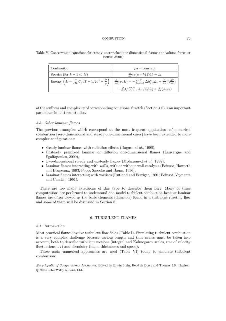
Table V. Conservation equations for steady unstretched one-dimensional flames (no volume forces orsource terms)
Continuity: ρu = constant
Species (for k = 1 to N) ∂∂x
(ρ(u + Vk)Yk) = ωk
Energy
„E =
R T
T0
CpdT + 1/2u2−
p
ρ
«∂
∂x(ρuE) = −
PN
k=1∆ho
f,kωk + ∂∂x
(λ ∂T∂x
)
−
∂∂x
(ρPN
k=1hs,kYkVk) + ∂
∂x(σxxu)
of the stiffness and complexity of corresponding equations. Stretch (Section 4.6) is an importantparameter in all these studies.
5.3. Other laminar flames
The previous examples which correspond to the most frequent applications of numericalcombustion (zero-dimensional and steady one-dimensional cases) have been extended to morecomplex configurations:
• Steady laminar flames with radiation effects (Daguse et al., 1996),• Unsteady premixed laminar or diffusion one-dimensional flames (Lauvergne and
Egolfopoulos, 2000),• Two-dimensional steady and unsteady flames (Mohammed et al., 1998),• Laminar flames interacting with walls, with or without wall catalysis (Poinsot, Haworth
and Bruneaux, 1993; Popp, Smooke and Baum, 1996),• Laminar flames interacting with vortices (Rutland and Ferziger, 1991; Poinsot, Veynante
and Candel, 1991).
There are too many extensions of this type to describe them here. Many of thesecomputations are performed to understand and model turbulent combustion because laminarflames are often viewed as the basic elements (flamelets) found in a turbulent reacting flowand some of them will be discussed in Section 6.
6. TURBULENT FLAMES
6.1. Introduction
Most practical flames involve turbulent flow fields (Table I). Simulating turbulent combustionis a very complex challenge because various length and time scales must be taken intoaccount, both to describe turbulent motions (integral and Kolmogorov scales, rms of velocityfluctuations,. . . ) and chemistry (flame thicknesses and speed).
Three main numerical approaches are used (Table VI) today to simulate turbulentcombustion:
Encyclopedia of Computational Mechanics. Edited by Erwin Stein, Rene de Borst and Thomas J.R. Hughes.
c© 2004 John Wiley & Sons, Ltd.
26 ENCYCLOPEDIA OF COMPUTATIONAL MECHANICS
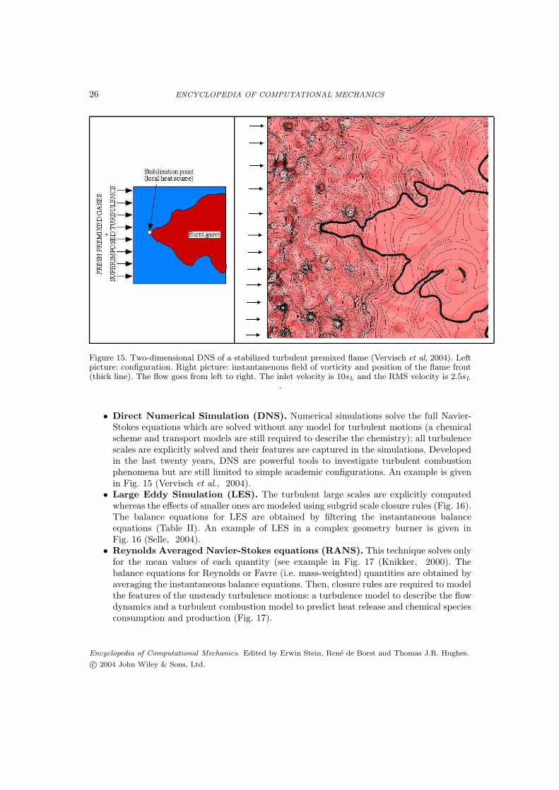
Figure 15. Two-dimensional DNS of a stabilized turbulent premixed flame (Vervisch et al, 2004). Leftpicture: configuration. Right picture: instantanenous field of vorticity and position of the flame front(thick line). The flow goes from left to right. The inlet velocity is 10sL and the RMS velocity is 2.5sL
.
• Direct Numerical Simulation (DNS). Numerical simulations solve the full Navier-Stokes equations which are solved without any model for turbulent motions (a chemicalscheme and transport models are still required to describe the chemistry): all turbulencescales are explicitly solved and their features are captured in the simulations. Developedin the last twenty years, DNS are powerful tools to investigate turbulent combustionphenomena but are still limited to simple academic configurations. An example is givenin Fig. 15 (Vervisch et al., 2004).
• Large Eddy Simulation (LES). The turbulent large scales are explicitly computedwhereas the effects of smaller ones are modeled using subgrid scale closure rules (Fig. 16).The balance equations for LES are obtained by filtering the instantaneous balanceequations (Table II). An example of LES in a complex geometry burner is given inFig. 16 (Selle, 2004).
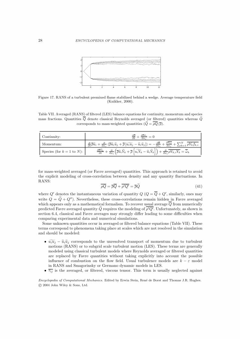
• Reynolds Averaged Navier-Stokes equations (RANS). This technique solves onlyfor the mean values of each quantity (see example in Fig. 17 (Knikker, 2000). Thebalance equations for Reynolds or Favre (i.e. mass-weighted) quantities are obtained byaveraging the instantaneous balance equations. Then, closure rules are required to modelthe features of the unsteady turbulence motions: a turbulence model to describe the flowdynamics and a turbulent combustion model to predict heat release and chemical speciesconsumption and production (Fig. 17).
Encyclopedia of Computational Mechanics. Edited by Erwin Stein, Rene de Borst and Thomas J.R. Hughes.
c© 2004 John Wiley & Sons, Ltd.

COMBUSTION 27
Table VI. Approaches for numerical simulations of turbulent combustion.
Approach Advantages Drawbacks
DNS - no models needed for - prohibitive numerical costs
turbulence/combustion interaction (fine grids, precise codes)
- tool to study models - limited to academic problems
LES - unsteady features - models required
- reduced modeling impact - 3D simulations required
(compared to RANS) - needs precise codes
- numerical costs
RANS - “coarse” numerical grid - only mean flow field
- geometrical simplification - models required
(2D flows, symmetry,...)
- “reduced” numerical costs
Figure 16. LES of an industrial gas turbine swirled combustor. Left: complete geometry. Right:instantaneous isosurface of temperature colored by velocity (Selle, 2004)).
Balance equations for RANS and LES are formally the same and involve similar unclosedquantities that must be modeled. The first ones are obtained by averaging instantaneousequations summarized in Table II when the second set is derived by combining theseinstantaneous equations with a filtering operator. As these techniques are emphasized in otherchapters of this encyclopedia, the attention is focused here on the specificity of combustion.Averaged or filtered balance equations for continuity, momentum and species mass fractionsare summarized in Table VII.
First, as usually done in variable density flows, numerical simulations in combustion solve
Encyclopedia of Computational Mechanics. Edited by Erwin Stein, Rene de Borst and Thomas J.R. Hughes.
c© 2004 John Wiley & Sons, Ltd.
28 ENCYCLOPEDIA OF COMPUTATIONAL MECHANICS
0 2 4 6 8 10 12
−2
−1
0
1
2
Figure 17. RANS of a turbulent premixed flame stabilized behind a wedge. Average temperature field(Knikker, 2000).
Table VII. Averaged (RANS) of filtered (LES) balance equations for continuity, momentum and species
mass fractions. Quantities Q denote classical Reynolds averaged (or filtered) quantities whereas eQcorresponds to mass-weighted quantities ( eQ = ρQ/ρ).
Continuity: ∂ρ
∂t+ ∂ρeui
∂xi= 0
Momentum: ∂∂t
ρeui + ∂∂xj
(ρeuieuj + ρ [ guiuj − euieuj ]) = −
∂p
∂xi+
∂τij
∂xj+
PN
k=1ρYkfk,i
Species (for k = 1 to N): ∂ρ eYk
∂t+ ∂
∂xi
“ρeui
eYk + ρh
guiYk − euieYk
i”+ ∂
∂xiρVk,iYk = ωk
for mass-weighted averaged (or Favre averaged) quantities. This approach is retained to avoidthe explicit modeling of cross-correlation between density and any quantity fluctuations. InRANS:
ρQ = ρQ + ρ′Q′ = ρQ (41)
where Q′ denotes the instantaneous variation of quantity Q (Q = Q + Q′, similarly, ones may
write Q = Q + Q′′). Nevertheless, these cross-correlations remain hidden in Favre averagedwhich appears only as a mathematical formalism. To recover usual average Q from numericallypredicted Favre averaged quantity Q requires the modeling of ρ′Q′. Unfortunately, as shown insection 6.4, classical and Favre averages may strongly differ leading to some difficulties whencomparing experimental data and numerical simulations.
Some unknown quantities occur in averaged or filtered balance equations (Table VII). Theseterms correspond to phenomena taking place at scales which are not resolved in the simulationand should be modeled:
• uiuj − uiuj corresponds to the unresolved transport of momentum due to turbulentmotions (RANS) or to subgrid scale turbulent motion (LES). These terms are generallymodeled using classical turbulent models where Reynolds averaged or filtered quantitiesare replaced by Favre quantities without taking explicitly into account the possibleinfluence of combustion on the flow field. Usual turbulence models are k − ε modelin RANS and Smagorinsky or Germano dynamic models in LES.
• τij is the averaged, or filtered, viscous tensor. This term is usually neglected against
Encyclopedia of Computational Mechanics. Edited by Erwin Stein, Rene de Borst and Thomas J.R. Hughes.
c© 2004 John Wiley & Sons, Ltd.

COMBUSTION 29
turbulent transport (this assumption is generally valid in RANS but questionable isLES) or simply modeled by adding a laminar viscosity to the turbulent one.
• ρVk,iYk is the averaged or filtered molecular diffusion of species k. As for the viscoustensor, this contribution is generally neglected against turbulent transport or modeledadding a laminar diffusion coefficient to the turbulent transport.
• uiYk−uiYk denotes the unresolved turbulent transport of species k. This term is generallydescribed using a gradient assumption, initially derived to model passive scalar turbulenttransport:
uiYk − uiYk = −νt
σk
∂Yk
∂xi
(42)
where νt is a turbulent kinematic viscosity, provided by the turbulence model andσk a turbulent Schmidt number. From a numerical point of view, this expression isattractive because the additional diffusivity νt helps to stabilize numerical simulations.Nevertheless, both theoretical analysis (see § 6.4), DNS and experiments have shownthat, in some situations, turbulent fluxes may have a sign opposite to the one predictedby Eq. (42), leading to so-called counter-gradient turbulent transport.
• ωk is the averaged, or filtered, reaction rate of species k. As the instantaneous reactionrate is highly non-linear (see § 3.5), ωk cannot be easily expressed from Arrhenius lawsand requires modeling.
Research in combustion modeling is largely devoted to the description of the mean reactionrate ωk. The first idea was to expand in Taylor series the expression (11) but this approachis not relevant because the convergence of this alternate series is very slow. This expansionalso introduces new unclosed quantities such as cross-correlations between mass fractions andtemperature fluctuations. Since this mathematical approach did not lead to meaningful results,most models have been based on physical analysis, as described in the following section.
6.2. Physical analysis - Combustion diagrams
As the mean reaction rate ωk cannot be found from a direct averaging of Arrhenius laws,combustion models are based on a more physical approach, based on an analysis of the flamestructure and various simplifying assumptions. Turbulent combustion involves various lengths,velocity and time scales describing turbulent flow field and chemical reactions. The Damkohlernumber compares the turbulent time scale τt and the chemical time scale τc :
Da =τt
τc
(43)
In the limit of high Damkohler numbers (Da � 1), the chemical time is short compared tothe turbulent time, corresponding to a thin reaction zone distorted and convected by the flowfield. The internal structure of the flame is not affected by turbulence and may be describedas a laminar flame element called flamelet, wrinkled and strained by the turbulence motions.
On the other hand, a low Damkohler (Da � 1) corresponds to a slow chemical reaction.Reactants and products are mixed by turbulent structures before reaction. In this perfectlystirred reactor limit (see § 5.1.2), the mean reaction rate is directly expressed from Arrheniuslaws using mean (or filtered) mass fractions and temperature. This is the only case where this
Encyclopedia of Computational Mechanics. Edited by Erwin Stein, Rene de Borst and Thomas J.R. Hughes.
c© 2004 John Wiley & Sons, Ltd.

30 ENCYCLOPEDIA OF COMPUTATIONAL MECHANICS
T = 300 K
T = 2000 K
turbulent flame
thickness
T = 2000 K
T = 300 K(a)
flameletpreheat zone
flameletreaction zone
Fresh gases
Burnt gases
T = 300 K
T = 2000 K
turbulent flame
thickness
T = 2000 K
T = 300 K
(b)
meanpreheat zone
mean reaction zone
Fresh gases
Burnt gases
T = 300 K
T = 2000 K
turbulent flame
thickness
T = 2000 K
T = 300 K
(c)
mean reaction zone
Fresh gases
Burnt gasesmeanpreheat zone
Figure 18. Turbulent premixed combustion regimes as identified by Borghi and Destriau, 1998: (a) Thinwrinkled flame (flamelet) regime; (b) thickened-wrinkled flame regime; (c) thickened flame regime.
procedure works because most practical situations correspond to high to medium values of theDamkohler numbers.§
In turbulent premixed flames, the chemical time scale τc may be estimated as the ratiobetween the flame thickness δL and the laminar flame speed SL. The turbulent time scalecorresponds to the integral length scale lt and is estimated as τt = lt/u′ where u′ is the rmsvelocity (or the square root of the turbulent kinetic energy). Then, the Damkohler numberbecomes:
Da =τt
τc
=ltδl
SL
u′(44)
where velocity (u′/SL) and length scale (lt/δL) ratios are identified. For large values ofthe Damkohler number (Da � 1), the flame front is thin and its structure is not affectedby turbulence motions. This regime is called flamelet regime or thin wrinkled flame regime(Fig. 18a). As the turbulence level increases, turbulent structures may affect the preheat zoneof the flame (Fig. 18b), corresponding to the thickened-wrinkled flame regime. If the turbulencelevel continues to increase (and Da to decrease), turbulent motions becomes sufficiently strongto affect the whole flame structure (thickened flame regime, Fig. 18c). These regimes aregenerally identified in a combustion diagram (Fig. 19). The previous analysis is due to Borghiand Destriau, 1998, but similar classifications may be found in the literature (Williams, 1985;Peters, 2000).
Such classifications are only qualitative and cannot be used to determine a combustionregime from the knowledge of turbulent (lt and u′) and chemical (δL and sL) scales. Various
§Note also that the definition of a chemical time scale τc is not unique: oxidation of the primary fuel correspondsto short values of τc and large values of Da but pollutant production or destruction such as CO oxidation orNOx formation are quite slower (large τc and small Da) leading to additional difficulties in characterizingturbulent flame regimes.
Encyclopedia of Computational Mechanics. Edited by Erwin Stein, Rene de Borst and Thomas J.R. Hughes.
c© 2004 John Wiley & Sons, Ltd.

COMBUSTION 31
1
2
3
4
5
678910
2
3
4
5
6789100
Ka = 1
Re = 100
Re = 10
Da =
1
1 10 100 1000
Thin wrinkled flame (flamelet)
Thickened / wrinkled flames
Thickened flames
Veynante et al.
Poinsot et al.
Figure 19. Turbulent premixed combustion diagram (Borghi and Destriau, 1998). Flame regimes areidentified as a function of the length scale (lt/δL) and velocity (u′/SL) ratios. The Klimov-Williamscriterion (Ka = 1) corresponds to a flame thickness δL equal to the Kolmogorov turbulent length scalelk. Below this line, the flame is thinner than any turbulent length scale. The flamelet limit derived byPoinsot, Veynante and Candel, 1991 from DNS is also plotted. The criterion proposed by Veynanteet al., 1997 to delineate between gradient (above) and counter-gradient (below) turbulent diffusion is
displayed for a heat release factor τ = Tb/Tu − 1 = 6.
assumptions are implicitly made to derive combustion diagrams. For example, turbulence issupposed to be homogeneous, isotropic and unaffected by heat release. Both direct numericalsimulations (Poinsot, Veynante and Candel, 1991) and experiments (Roberts et al., 1993)show that the flamelet regime is larger than predicted by these qualitative analysis. Anessential mechanism revealed by DNS is that small turbulent scales, which are supposed inclassical theories to have the strongest effects on flames, have small lifetimes because of viscousdissipation and therefore only limited effects on combustion. Fig. 19 shows the flamelet regimelimit obtained from DNS (Poinsot, Veynante and Candel, 1991) and the criterion delineatingbetween gradient and counter gradient turbulent transport (§ 6.4) proposed by Veynante etal., 1997.
Identification of combustion regimes is more difficult in non-premixed turbulent flames forwhich estimating chemical times or scales is more ambiguous. Nevertheless some classificationshave been proposed (Borghi and Destriau, 1998; Cuenot and Poinsot, 1994; Peters, 2000;Poinsot and Veynante, 2001; Veynante and Vervisch, 2002) but will not be discussed here.
Model derivations are usually based on the classification of the combustion regimes. Forexample, in the flamelet regime, the flame front may be identified as an infinitely thin flamesurface having the inner structure of a laminar flame but convected and distorted by turbulencemotions. Various points of view have been developed by modelers but are closer than usuallyexpected as shown by Veynante and Vervisch, 2002. In the following, the basic tools formodeling are identified and discussed.
Encyclopedia of Computational Mechanics. Edited by Erwin Stein, Rene de Borst and Thomas J.R. Hughes.
c© 2004 John Wiley & Sons, Ltd.
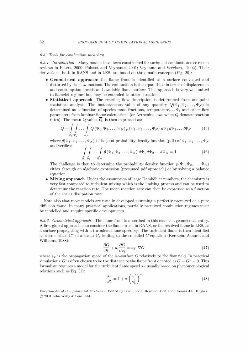
32 ENCYCLOPEDIA OF COMPUTATIONAL MECHANICS
6.3. Tools for combustion modeling
6.3.1. Introduction Many models have been constructed for turbulent combustion (see recentreviews in Peters, 2000; Poinsot and Veynante, 2001; Veynante and Vervisch, 2002). Theirderivations, both in RANS and in LES, are based on three main concepts (Fig. 20):
• Geometrical approach: the flame front is identified to a surface convected anddistorted by the flow motions. The combustion is then quantified in terms of displacementand consumption speeds and available flame surface. This approach is very well suitedto flamelet regimes but may be extended to other situations.
• Statistical approach. The reacting flow description is determined from one-pointstatistical analysis. The instantaneous value of any quantity Q(Ψ1, Ψ2, . . . , ΨN ) isdetermined as a function of species mass fractions, temperature,. . . Ψi and other flowparameters from laminar flame calculations (or Arrhenius laws when Q denotes reactionrates). The mean Q value, Q, is then expressed as:
Q =
∫
Ψ1
∫
Ψ2
. . .
∫
ΨN
Q (Ψ1, Ψ2, . . . , ΨN ) p (Ψ1, Ψ2, . . . , ΨN) dΨ1 dΨ2 . . . dΨN (45)
where p(Ψ1, Ψ2, . . . , ΨN) is the joint probability density function (pdf) of Ψ1, Ψ2, . . . , ΨN
and verifies: ∫
Ψ1
∫
Ψ2
. . .
∫
ΨN
p (Ψ1, Ψ2, . . . , ΨN ) dΨ1 dΨ2 . . . dΨN = 1 (46)
The challenge is then to determine the probability density function p(Ψ1, Ψ2, . . . , ΨN)either through an algebraic expression (presumed pdf approach) or by solving a balanceequation.
• Mixing approach. Under the assumption of large Damkohler numbers, the chemistry isvery fast compared to turbulent mixing which is the limiting process and can be used todetermine the reaction rate. The mean reaction rate can then be expressed as a functionof the scalar dissipation rate.
Note also that most models are usually developed assuming a perfectly premixed or a purediffusion flame. In many practical applications, partially premixed combustion regimes mustbe modelled and require specific developments.
6.3.2. Geometrical approach The flame front is described in this case as a geometrical entity.A first global approach is to consider the flame brush in RANS, or the resolved flame in LES, asa surface propagating with a turbulent flame speed sT . The turbulent flame is then identifiedas a iso-surface G∗ of a scalar G, leading to the so-called G-equation (Kerstein, Ashurst andWilliams, 1988):
∂G
∂t+ ui
∂G
∂xi
= sT |∇G| (47)
where sT is the propagation speed of the iso-surface G relatively to the flow field. In practicalsimulations, G is often chosen to be the distance to the flame front denoted as G = G∗ = 0. Thisformalism requires a model for the turbulent flame speed sT usually based on phenomenologicalrelations such as Eq. (1):
sT
s0L
= 1 + α
(u′
s0L
)n
(48)
Encyclopedia of Computational Mechanics. Edited by Erwin Stein, Rene de Borst and Thomas J.R. Hughes.
c© 2004 John Wiley & Sons, Ltd.
COMBUSTION 33
Figure 20. Various approaches used to derive turbulent combustion models.
where u′ is the rms of the turbulent velocity and α and n two model parameters. From anumerical point of view, the G-equation formalism can be difficult to handle: it creates cusps,generally avoided by adding diffusion, and requires sophisticated front tracking methods.
Another formalism is based on the flame surface density Σ, measuring the available flamesurface per unit volume (Marble and Broadwell, 1977). Reaction rates are then written as:
ωk = 〈Vk〉Σ (49)
where 〈Vk〉 is the mean reaction rate of species k per unit of flame area, generally identifiedto the laminar reaction rate. Under flamelet assumptions, this approach separates complexchemistry features incorporated in 〈Vk〉 through flamelet libraries from flame / turbulenceinteractions described by Σ. The flame surface density may be determined by:
• An algebraic expression such as (Bray, Champion and Libby, 1989):
Σ = gΘ(1 − Θ
)
σyLy
(50)
in premixed combustion. σy is an orientation factor, assumed to be constant, g a modelconstant and Ly a flame wrinkling length scale related to the turbulence integral scalelt. Other expressions are based on fractal analysis (Gouldin, Bray and Chen, 1989).
• A balance equation. Marble and Broadwell, 1977 have first proposed such an equationfrom phenomenological arguments. An exact, but unclosed, Σ-balance equation may bederived (Trouve et al., 1994; Veynante and Vervisch, 2002):
∂Σ
∂t+
∂
∂xi
(〈ui〉sΣ) +∂
∂xi
[〈sdni〉sΣ] =
⟨(δij − ninj)
∂ui
∂xj
⟩
s
Σ +
⟨sd
∂ni
∂xi
⟩
s
Σ (51)
where sd is the displacement speed of the flame, ni are the component of the unit vectorn normal to the flame front (in premixed combustion, n is chosen pointing towards thefresh gases: n = −∇Θ/ |∇Θ| where Θ is the progress variable described in Section 4.3.The flame front curvature is given by ∂ni/∂xi. 〈〉s denotes the surface averaged operator(i.e. average along the flame surface). The three terms in the LHS of the Σ balance
Encyclopedia of Computational Mechanics. Edited by Erwin Stein, Rene de Borst and Thomas J.R. Hughes.
c© 2004 John Wiley & Sons, Ltd.

34 ENCYCLOPEDIA OF COMPUTATIONAL MECHANICS
equation (51) correspond respectively to unsteady effects, to flame surface convection bythe flow and normal flame propagation. The first term in the RHS expresses the action ofthe tangential strain rate on the flame surface and the last term corresponds to combinedpropagation/curvature effects. All these terms can be modelled (Bruneaux, Poinsot andFerziger , 1997; Poinsot and Veynante, 2001) and the Σ equation is routinely used inmany combustion codes.
6.3.3. Statistical approach In this formalism, the challenge is to determine the jointprobability density function p in Eq. (45). Two main approaches are used:
• Presumed probability density function. The shape of the function is given apriori and depends on the first moments of the described variable. Various shapes maybe used: if log-normal distributions are retained to describe turbulence characteristics(turbulence times, strain rates), β-functions are generally chosen for chemical quantities,when depending on only one variable, progress variable Θ for premixed combustion ormixture fraction z for diffusion flames:
p (Θ) =1
B (a, b)Θa−1 (1 − Θ)
b−1with B (a, b) =
1∫
0
Θa−1 (1 − Θ)b−1
dΘ (52)
The parameters a and b are given by the two first moments of Θ:
a = Θ
Θ(1 − Θ
)
Θ′′2− 1
; b =
a
Θ− a (53)
A model is required for the variance Θ′′2 of the variable Θ. In RANS, a balance equation
is usually solved for Θ′′2 whereas similarity arguments are retained to estimate thisvariance in LES. This formalism, widely used in practical simulations, is very difficult toextend to multi-variables pdf.¶
• Balance equation. A balance equation may be derived (Pope, 1985; Dopazo, 1994):
ρ∂p
∂t+ ρuk
∂p
∂xk
= −∂
∂xk
[ρ (u′′
k|Y = Ψ) p]
︸ ︷︷ ︸Turbulent convection
− ρ
N∑
i=1
∂
∂Ψi
(ωi (Ψ1, Ψ2, . . . , ΨN ) p)
︸ ︷︷ ︸Chemical reaction
− ρN∑
i=1
N∑
j=1
∂
∂Ψi
∂
∂Ψj
[D
(∂Yi
∂xk
∂Yj
∂xk
|Y = Ψ
)p
]
︸ ︷︷ ︸Molecular mixing
(54)
(Q|Y = Ψ) correspond to conditional averaging of quantity Q for the sampling valuesΨi. In this equation, the chemical reaction term is closed and does not require modeling
¶Sometimes, a statistical variable independence is assumed to evaluate the pdf simply: ep(Y1, Y2, . . . , T ) ≈ep(Y1)ep(Y2) . . . ep(T ). This assumption is clearly wrong in most reacting flows where mass fractions andtemperature are not independent.
Encyclopedia of Computational Mechanics. Edited by Erwin Stein, Rene de Borst and Thomas J.R. Hughes.
c© 2004 John Wiley & Sons, Ltd.

COMBUSTION 35
because the reaction rate depends only on quantities given in the pdf. This makespdf approaches attractive when complex chemical schemes are needed. Unfortunately,the mixing term, requiring two-points information, is unclosed and should be modeled.Solving the pdf balance equation needs large computational efforts, limiting its use toresearch numerical simulations.
6.3.4. Mixing approach For large Damkohler numbers or flamelet regimes, the turbulentmixing appears as the limiting process. The rate of mixing may be estimated as the temporalevolution of the variance of a scalar such as the progress variable Θ or the mixing fraction z.
Neglecting mean scalar gradients, the balance equation for z′′2 may be written:
dρz′′2
dt≈ −ρχ (55)
where χ is the scalar dissipation rate:
ρχ = ρD∂z
∂xi
∂z
∂xi
≈ ρD∂z′′
∂xi
∂z′′
∂xi
(56)
The scalar dissipation rate measures directly the rate of decay of fluctuations via turbulentmixing. Conditional scalar dissipation rates are found in the balance equation for theprobability density function (Eq. 54). When mixing limits the turbulent combustion, thereaction rate is modeled as being proportional to the scalar dissipation rate χ. Eq. (55) isused to model χ as the ratio of the variance and a turbulent time scale τt (a balance equationmay be derived for χ). The well-known Eddy-Break-Up model for turbulent premixed flameis based on this formalism writing:
ωk = CEBUρΘ′′2
τt
(57)
where CEBU is a model constant. For a bimodal progress variable Θ (i.e. Θ = 0 or Θ = 1),
Θ′′2 = Θ(1 − Θ) and the reaction rate for the progress variable Θ is expressed as:
ωΘ = CEBUρΘ(1 − Θ
)
τt
(58)
6.4. Bray-Moss-Libby analysis
Bray and Moss, 1977 have derived a useful analysis in the limit of infinitely thin flame frontsin premixed combustion in a RANS context. This approach leads to the so-called BML(Bray-Moss-Libby) model but is presented here to evidence some difficulties in combustiondescription. These authors assume that the the flame front is so thin that the temperature Θ(section 4.3) exhibits only two states (burnt or unburnt) so that the pdf of Θ is:
p (Θ) = α δ (Θ) + β δ (1 − Θ) (59)
where δ is the Dirac-δ function and α and β are respectively the probability to have fresh andfully burnt gases (α + β = 1). The mean value Q of any quantity f is directly given by:
Q =
∫ 1
0
f(Θ)p(Θ) dΘ = α Qu
+ β Qb
(60)
Encyclopedia of Computational Mechanics. Edited by Erwin Stein, Rene de Borst and Thomas J.R. Hughes.
c© 2004 John Wiley & Sons, Ltd.

36 ENCYCLOPEDIA OF COMPUTATIONAL MECHANICS
1.0
0.8
0.6
0.4
0.2
0.0
Rey
nold
s av
erag
e
1.00.80.60.40.20.0
Favre (mass-weighted) average
τ 0 1 2 4 6 10
Figure 21. Reynolds average temperature Θ as a versus Favre average temperature eΘ for various valuesof the heat release factor τ , assuming a bimodal distribution (Θ = 0 or Θ = 1) for Θ (Eq. 63).
where Qu
and Qb
denote the conditional averages of Q in fresh and burnt gases respectively.Applying relation (60) to Θ, ρΘ and ρ gives:
Θ = β ; ρΘ = ρΘ = ρbΘ ; ρ = (1 − β) ρu + βρb (61)
where ρu and ρb are the density of fresh and burnt gases respectively. Introducing the heatrelease factor τ measuring the thermal expansion: τ = ρu/ρb−1 = Tb/Tu−1, where Tu and Tb
are the fresh and burnt gases temperatures respectively, and combining relations (61) providean expression for the probability α and β:
α =1 − Θ
1 + τΘ; β =
(1 + τ) Θ
1 + τΘ(62)
This derivation leads to the following comments:
• The probabilities α and β to be in fresh and burnt gases are directly determined as afunction of the Favre averaged progress variable Θ (Eq. 62).
• The Reynolds averaged progress variable Θ measures only the probability to be in burntgases (Θ = β).
• Under the assumption of an infinitely thin flame front, and a bimodal distribution of theprogress variable Θ, a direct relation is obtained between Reynolds (Θ) and Favre, or
mass-weighted (Θ) averages:
Θ = β =(1 + τ) Θ
1 + τΘ(63)
showing that substantial differences between Θ and Θ, may be encountered (Fig. 21).These differences make comparisons between numerical simulations and experimentaldata difficult.
Another interesting relation is to apply Eq. (60) to ρQ:
Q = αρu
ρQ
u+ β
ρb
ρQ
b=(1 − Θ
)Q
u+ ΘQ
b(64)
Encyclopedia of Computational Mechanics. Edited by Erwin Stein, Rene de Borst and Thomas J.R. Hughes.
c© 2004 John Wiley & Sons, Ltd.

COMBUSTION 37
The Favre averaged value of any quantity Q is a weighted averaged of mean values in fresh andburnt gases. The weighting coefficient is the progress variable θ (i.e. the reduced temperature).This simple relation has consequences on the turbulent fluxes. The turbulent fluxes of Θ iseasily expressed as:
ρ(uiΘ − uiΘ
)= ρΘ
(1 − Θ
) (ub
i − uui
)(65)
For a statistically one-dimensional turbulent premixed flame propagating along the x-axisoriented towards burnt gases, Eq. (65) may predict a positive scalar flux as ub
i is expected tobe larger than uu
i because of thermal expansion. On the other hand, usual gradient assumptions(Eq. 42) lead to a negative flux. This counter-gradient turbulent transport (i.e. in the directionopposite to the one predicted by classical gradient assumptions) is generally explained bydifferential buoyancy effects induced by pressure gradients acting on heavy cold fresh gasesand light hot burnt ones. This phenomenon has been observed both experimentally (Shepherd,Moss and Bray, 1982) and in direct numerical simulations (Veynante et al., 1997). A fulldiscussion of counter-gradient turbulent transport is out of the scope of this chapter but thissituation, occurring for low turbulence levels, high thermal expansion and confined flames,is generally neglected in practical computations. One reason for this is that usual gradientassumptions lead to diffusion terms which stabilize numerical simulations. Another reasonis that taking into account counter-gradient turbulent transport requires to solve balanceequations for turbulent fluxes uiΘ − uiΘ and for Reynolds stresses uiuj − uiuj , adding nineequations in three-dimensional simulations.
Applied to Reynolds stresses (turbulent fluxes of momentum), Eq. (64) gives:
(uiuj − uiuj) =(1 − Θ
) (uiu
uj − uu
i uuj
)
︸ ︷︷ ︸fresh gases
+ Θ(uiu
bj − ub
iubj
)
︸ ︷︷ ︸burnt gases
+ Θ(1 − Θ
) (ub
i − uui
) (ub
j − uuj
)
︸ ︷︷ ︸intermittency
(66)Reynolds stresses, and turbulent kinetic energy, then appear as a weighted average of fresh andburnt gas Reynolds stresses, corresponding to actual turbulence, and to an additional termdue to intermittency between fresh and burnt gases. Nevertheless, in practical simulations,intermittency is not explicitly taken into account and turbulence is generally described usingclassical models derived for non reacting flows where Reynolds averages are replaced by Favreaverages.
REFERENCES
Abdel-Gayed R., Bradley D., Hamid M. and Lawes M. Lewis number effects on turbulentburning velocity.Proceedings of the Combustion Institute 1984; 20: 505-512.
Abdel-Gayed R. and Bradley D. Combustion regimes and the straining of turbulent premixedflames.Combustion and Flame 1989; 76: 213-218.
Aung K., Hassan M. and Faeth G. Effects of pressure and nitrogen dilution on flame stretchinteractions of laminar premixed hydrogen air flames. Combustion and Flame 1998; 112:1-15.
Encyclopedia of Computational Mechanics. Edited by Erwin Stein, Rene de Borst and Thomas J.R. Hughes.
c© 2004 John Wiley & Sons, Ltd.

38 ENCYCLOPEDIA OF COMPUTATIONAL MECHANICS
Ashurst W., Peters N. and Smooke M. Numerical simulation of turbulent flame structure withnon-unity Lewis number. Combustion Science and Technology 1987; 53: 339-375.
Baum M., Thevenin D. and Poinsot T. Accurate boundary conditions for multicomponentreactive flows. Journal of Computational Physics 1994; 116: 247-261.
Bilger R. Turbulent diffusion flames. Annual Review Fluid Mechanics 1989; 21:101.
Bird R., Stewart W. and Lightfoot E. Transport Phenomena, Second Edition 2002; J. Wiley.
Borghi R. and Destriau M. Combustion and flames, chemical and physical principles 1998;Editions Technip, Paris.
Bray K.N.C. and Moss J.B. A unified statistical model of premixed turbulent flame. ActaAstronautica 1977; 4:291-319.
Bray K.N.C., Champion M. and Libby P.A. The interaction between turbulence and chemistryin premixed turbulent flames. Turbulent Reaction Flows, Lecture notes in engineering,Springer Verlag 1989; 541-563.
Bruneaux G., Poinsot T. and Ferziger J. Premixed flame-wall interaction in a turbulent channelflow: budget for the flame surface density evolution equation and modelling. Journal ofFluid Mechanics 1997; 349: 191-219.
Candel S. and Poinsot T. Flame stretch and the balance equation for the flame surface area.Combustion Science and Technology 1990; 70: 1-15.
Clavin P. Dynamics of flame fronts in premixed gases: from flames to detonation.Proceedingsof the Combustion Institute 2000; 28: 569-585.
Cuenot B. and Poinsot T. Effects of curvature and unsteadiness in diffusion flames. Implicationsfor turbulent diffusion flames. Proceedings of the Combustion Institute 1994; 25: 1383-1390.
Crocco L. Aspects of combustion instability in liquid propellant rocket motors. Part I Journalof the Americal Rocket Society 1951; 21: 163-178.
Crocco L. Aspects of combustion instability in liquid propellant rocket motors. Part II Journalof the Americal Rocket Society 1952; 22: -.
Daguse T., Croonenbroek T., Darabiha N., Rolon J.C. and Soufiani A. Study of radiativeeffects on laminar counterflow H2 O2 N2 diffusion flames. Combustion and Flame 1996;106: 271-287.
Damkholer G. Z. Elektrochem. 1940; 46: 610.
Darabiha N. and Candel S. The influence of the temperature on extinction and ignition limitsof strained hydrogen-air diffusion flames. Combustion Science and Technology 1992; 86:67-85.
Dold, J W. Analysis of a slowly varying triple flame Combustion and Flame 1989; 76: 71-88.
Domingo P. and Vervisch L. Triple flames and partially premixed combustion in autoignitionof nonpremixed mixture.Proceedings of the Combustion Institute 1996; 26: 233-240.
Dopazo C. Recent developments in pdf methods. Turbulent Reacting Flows, Academic Press,1994, 375-474.
Encyclopedia of Computational Mechanics. Edited by Erwin Stein, Rene de Borst and Thomas J.R. Hughes.
c© 2004 John Wiley & Sons, Ltd.
COMBUSTION 39
Dowdy D., Smith D. and Taylor S. The use of expanding spherical flames to determine burningvelocities and stretch effects in hydrogen/air mixtures. Proceedings of the CombustionInstitute 1990; 23: 325-332.
Duclos, J.M., Veynante, D. and Poinsot, T. A comparison of flamelet models for premixedturbulent combustion. Combustion and Flame 1995; 95: 101-117.
Roberts W.L., Driscoll J.F., Drake M.C. and Goss L.P. Images of a quencing of a flame bya vortex: to quantify regime of turbulent combustion. Combustion and Flame 1993; 94:58-69.
Egolfopoulos F. and Law C. Further considerations on the determination of laminar flamespeeds with the counterflow twin flame technique. Proceedings of the Combustion Institute1994; 25: 1341-1347.
Ern A. and Giovangigli V. Multicomponent Transport Algorithms 1994; Lecture Notes inPhysics, Springer Verlag.
Gardiner W. Gas-phase combustion chemistry 2000; Springer Verlag.
Ghosal S. and Vervisch L. Theoretical and numerical investigation of a symmetrical tripleflame using a parabolic flame tip approximation. Journal of Fluid Mechanics 2000; 415:227-260.
Giovangigli V. Multicomponent Flow Modeling 1999; Modeling and Simulation in Science,Engineering and Technology, Birkhauser.
Giovangigli V. and Smooke M. Extinction of strained premixed laminar flames with complexchemistry. Combustion Science and Technology 1987; 53: 23-49.
Glassman I. Combustion 1977; Academic Press.
Gouldin F. C. Combustion intensity and burning rate integral of premixed flames.Proceedingsof the Combustion Institute 1996; 26: 381-388.
Gouldin F. C., Bray K.N.C. and Chen J.Y. Chemical closure model for fractal flamelets.Combustion and Flame 1989; 77: 241.
Hirschfelder J., Curtiss C. and Byrd R. Molecular theory of gases and liquids 1969; John Wiley.
Hottel H. C. and Hawthorne W. R. Diffusion in laminar flame jets.Proceedings of theCombustion Institute 1949; 3: 254-266.
Ishizuka S. and Law C. An experimental study of extinction and stability of stretched premixedflames Proceedings of the Combustion Institute 1982; 19: 327-335.
Kee R., Grcar J., Smooke M. and Miller J. PREMIX: A Fortran program for modeling steadylaminar one-dimensional flames 1985; SAND85-8240, Sandia National Laboratories.
Keller J. O., Bramlette T., Barr P. K. and Alvarez J. R. NOx and CO emissions from a pulsecombustion operating in a lean premixed mode. Combustion and Flame 1994; 99: 460-466.
Keller J. O. and Saito T. Measurements of the combusting flow in a pulse combustor.Combustion Science and Technology 1987; 53: 137.
Kerstein A.R., Ashurst W. and Williams F.A. Field equation for interface propagation in anunsteady homogeneous flow field. Physical Review A 1988; 37: 2728-2731.
Encyclopedia of Computational Mechanics. Edited by Erwin Stein, Rene de Borst and Thomas J.R. Hughes.
c© 2004 John Wiley & Sons, Ltd.
40 ENCYCLOPEDIA OF COMPUTATIONAL MECHANICS
Kioni P. N., Rogg B., Bray K. N. C. and Linan A. Flame spread in laminar mixing layers: thetriple flame. Combustion and Flame 1993; 95: 276.
Kioni P. N., Bray K. N. C., Greenhalgh D. A. and Rogg B. Experimental and Numericalstudies of a triple flame. Combustion and Flame 1998; 116: 192-206.
Knikker R. Analyse experimentale de la combustion turbulente premelangee pour la simulationaux grandes echelles. PhD Thesis, Ecole Centrale de Paris, France 2000.
Kuo K. Principles of Combustion 1986; John Wiley.
Lauvergne R. and Egolfopoulos F.Unsteady response of C3H8 laminar premixed flamessubmitted to mixture composition oscillations. Proceedings of the Combustion Institute2000; 28: 1841-1850.
Law C. Dynamics of stretched flames. Proceedings of the Combustion Institute 1988; 22: 1381-1402.
Linan A. and Crespo A. An asymptotic analysis of unsteady diffusion flames for large activationenergies. Combustion Science and Technology 1976; 14: 95-117.
Linan A., Orlandi P., Verzicco R. and Higuera F. J. Effects of non-unity Lewis numbers indiffusion flames. Proceedings of the CTR Summer Program, Stanford University 1994;5-18.
Marble F.E. and Broadwell J.E. The coherent flame model for turbulent chemical reaction.Tech. report TRW-9-PU, Project Squid, 1977.
Mastorakos E., Baritaud T. A. and Poinsot T J. Numerical simulations of autoignition inturbulent mixing flows. Combustion and Flame 1997; 109: 198-223.
Matalon M. and Matkowsky B. Flames as gasdynamic discontinuities. Journal of FluidMechanics 1982; 124: 239.
Miller J. Theory an dmodelingin combustion chemistry. Proceedings of the CombustionInstitute 2000; 26: 461-480.
Mohammed R., Tanoff M., Smooke M. and Schaffer A. Computational and experimentalstudy of a forced, time varying, axisymmetric, laminar diffusion flame. Proceedings ofthe Combustion Institute 1998; 27: 693-702.
Muniz L. and Mungal M. G. Instantaneous flame-stabilization velocities in lifted-jet diffusionflames. Combustion and Flame 1997; 111: 16-31.
Oefelein J. and Yang V. Modeling high pressure mixing and combustion processes in liquidrocket engines.. Propulsion and Power 1998; 14, 5: 843-857.
Oran E. and Boris J. Numerical simulation of reactive flow 1987; Elsevier.
Peters N. Laminar diffusion flamelet models in non-premixed turbulent combustion.Progressin Energy and Combustion Sciences 1984; 10: 319-339.
Peters N. Turbulent combustion 2000; Cambridge University Press.
Poinsot T. Comments on ‘Effects of pressure and nitrogen dilution on flame stretch interactionsof laminar premixed hydrogen air flames’ by Aung et al. Combustion and Flame 1998;113: 279-284.
Encyclopedia of Computational Mechanics. Edited by Erwin Stein, Rene de Borst and Thomas J.R. Hughes.
c© 2004 John Wiley & Sons, Ltd.
COMBUSTION 41
Poinsot T., Echekki T. and Mungal M. A study of the laminar flame tip and implicationsfor premixed turbulent combustion. Combustion Science and Technology 1992; 81 (1-3):45-73.
Poinsot T., Haworth D. and Bruneaux G. Direct simulation and modelling of flame-wallinteraction for premixed turbulent combustion. Combustion and Flame 1993; 95: 118-133.
Poinsot T. and Lele S. Boundary conditions for direct simulations of compressible viscousflows. Journal of Computational Physics 1992; 101: 104-129.
Poinsot T., Trouve A. and Candel S. Application of direct numerical simulation to premixedturbulent combustion. Progress in Energy and Combustion Sciences 1996; 21: 531-576.
Poinsot T., Trouve A., Veynante D., Candel S. and Esposito E. Vortex driven acousticallycoupled combustion instabilities. Journal of Fluid Mechanics 1987; 177: 265-292.
Poinsot T. and Veynante D. Theoretical and numerical combustion 2001; R.T. Edwards.
Poinsot T., Veynante D. and Candel S. Quenching processes and premixed turbulentcombustion diagrams. Journal of Fluid Mechanics 1991; 228: 561-605.
Pope S.B. pdf methods for turbulent reacting flows. Progress in Energy and CombustionScience 1985; 19: 119-192.
Popp P., Smooke M. and Baum M. Heterogeneous/homogeneous reactions and transportcoupling during flame-wall interaction. Proceedings of the Combustion Institute 1996; 26:2693-2700.
Rayleigh L. The explanation of certain acoustic phenomena. Nature 1878; 18: 319-321.
Rutland C. and Ferziger J.Simulation of flame-vortex interactions. Combustion and Flame1991; 91: 343-360.
Selle L. Simulation aux grandes echelles des interactions flamme / acoustique dans unecoulement vrille. PhD Thesis, INP Toulouse, France 2004.
Shepherd I.G., Moss J.B. and Bray K.N.C. Turbulent transport in a confined premixed flame.Proceedings of the Combustion Institute 1982; 19: 423-431.
Stull D. and Prophet H. JANAF thermochemical tables, 2nd Edition NSRDS-NBS 37, USNational Bureau of Standards, 1971.
Trouve A. and Poinsot T. The evolution equation for the flame surface density.Journal of FluidMechanics 1994; 278: 1-31.
Turns S.R. An introduction to combustion, concepts and applications 1996; Mc Graw-Hill,Series in Mechanical Engineering.
Vervisch L., Hauguel R., Domingo P. and Rullaud M.Three facets of turbulent combustionmodelling: DNS of premixed V-flame, LES of lifted nonpremixed flame and RANS ofjet-flame. Journal of Turbulence 2004; 5: 004.
Veynante D., Trouve A., Bray K. N. C. and Mantel T. Gradient and counter-gradient scalartransport in turbulent premixed flames. Journal of Fluid Mechanics 1997; 332: 263-293.
Veynante D. and Vervisch L. Turbulent combustion modeling. Progress in Energy andcombustion science 2002; 28(3): 193-266.
Encyclopedia of Computational Mechanics. Edited by Erwin Stein, Rene de Borst and Thomas J.R. Hughes.
c© 2004 John Wiley & Sons, Ltd.

42 ENCYCLOPEDIA OF COMPUTATIONAL MECHANICS
Westbrook C. Chemical kinetics of hydrocarbon ignition in practical combustion systems.Proceedings of the Combustion Institute 2000; 28: 1563-1579.
Williams F. Combustion theory 1985; Benjamin Cummings.
Yakhot V., Orszag C. G., Thangam S., Gatski T. B. and Speziale C. G. Development ofturbulence models for shear flows by a double expansion technique. Physics of Fluids1992; 4: 1510.
Encyclopedia of Computational Mechanics. Edited by Erwin Stein, Rene de Borst and Thomas J.R. Hughes.
c© 2004 John Wiley & Sons, Ltd.