COMPARISON OF CENTRALIZED ANDDECENTRALIZED SCHEDULING ALGORITHMSUSING GSSIM SIMULATION ENVIRONMENT

Marcin Krystek, Krzysztof Kurowski, Ariel OleksiakPoznan Supercomputing and Networking CenterNoskowskiego 1061-704 Poznan, Polandmkrystek,krzysztof.kurowski,ariel@man.poznan.pl

Krzysztof RzadcaLIG, Grenoble University51, avenue Jean Kuntzmann38330 Montbonnot Saint Martin, Franceand Polish-Japanese Institute of Information TechnologyKoszykowa 8602-008 Warsaw, Polandrzadca@imag.fr

Abstract Various models and architectures for scheduling in grids may be foundboth in the literature and in practical applications. They differ in thenumber of scheduling components, their autonomy, general strategies,and the level of decentralization. The major aim of our research is tostudy impact of these differences on the overall performance of a Grid.To this end, in the paper we compare performance of two specific Gridmodels: one centralized and one distributed. We use GSSIM simula-tor to perform accurate empirical tests of algorithms. This paper is astarting point of an experimental study of centralized and decentral-ized approaches to Grid scheduling within the scope of the CoreGridResource Management and Scheduling Institute.

Keywords: Decentralized scheduling, scheduling architecture, scheduling algorithms,grid, GSSIM simulator

2

1. IntroductionDecentralization is a key feature of any architectural part of the grid,

a system that is crossing organizational boundaries [7]. Nevertheless,standard approaches to scheduling, both theoretical and practical, con-cern mainly centralized algorithms. In large-scale grids, the centralizedapproach is clearly unfeasible. Firstly, centralized scheduling requiresaccurate, centralized information about the state of the whole system.Secondly, sites forming the grid maintain some level of autonomy, yetclassic algorithms implicitly assume a complete control over individualresources.

We model the grid as an agreement to share resources between in-dependent organizations. An organization is an entity that groups acomputational resource (a cluster) and a group of users that submitjobs. Each organization, by granting access to its resource, in returnexpects that its jobs will be treated fairly in the system.

In the paper, we compare two classes of scheduling algorithms, cen-tralized and decentralized. In centralized scheduling, one grid schedulermaintains a complete control over the clusters. All the jobs are submit-ted through the grid scheduler. In contrast, in decentralized scheduling,organizations maintain (limited) control over their schedules. Jobs aresubmitted locally, but they can be migrated to another cluster, if thelocal cluster is overloaded. The possibilities of migration are, however,limited, so that migrated jobs do not overload the host system.

The aim of this paper is to compare performance centralized anddecentralized scheduling algorithms. Using GSSIM simulation environ-ment, we perfom realistic simulation of example scheduling algorithmsthat use both approaches, and compute various performance measuresof jobs.

In literature, decentralization has two distinct meanings in grid sys-tems, composed of resources under different administrative domains [7]:the decentralization of the algorithm or the decentralization of the op-timization goals. A decentralized algorithm does not need complete, ac-curate information about the system. An algorithm with decentralizedgoals optimizes many performance measures of different stakeholders ofthe system. Classic scheduling algorithm are centralized algorithms thatoptimize a centralized goal, such as the average completion time of jobsor the makespan. Such scheduling problems have been thoroughly stud-ied, both theoretically [2]and empirically [6]. Decentralized algorithmsoptimizing decentralized goals include mainly economic approaches [3].Decentralized algorithms optimizing system-level goal include e.g. [11],that proposes a load-balancing algorithm for divisible task model. Fi-

Comparison of Centralized and Decentralized Scheduling 3

nally, in optimization of decentralized goals with a centralized algorithm,multi-objective algorithms are usually used [13, 10].

The paper is organized as follows. The architecture of the schedulingsystem and algorithms for centralized and decentralized implementationsare proposed in Section 2. Section 3 contains a description of GSSIM,the simulation environment. Section 4 presents results of experiments.

2. Scheduling AlgorithmsIn this section we present the model of the grid and scheduling algo-

rithms. In the first case, we assume that there is a single grid sched-uler while local schedulers are not autonomous, i.e. they must acceptdecisions of a grid scheduler. In the second approach, there is no cen-tral grid scheduler and local schedulers are autonomous. However, theymust obey certain rules agreed between organizations. In both cases,jobs come from users from considered organizations, i.e. there are noexternal jobs. The next sections contains used notation and details ofalgorithms.

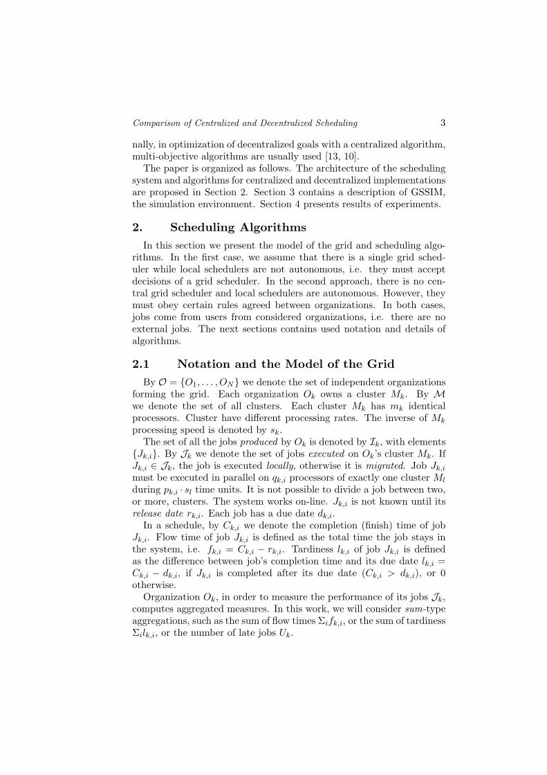
2.1 Notation and the Model of the GridBy O = {O1, . . . , ON} we denote the set of independent organizations

forming the grid. Each organization Ok owns a cluster Mk. By Mwe denote the set of all clusters. Each cluster Mk has mk identicalprocessors. Cluster have different processing rates. The inverse of Mk

processing speed is denoted by sk.The set of all the jobs produced by Ok is denoted by Ik, with elements

{Jk,i}. By Jk we denote the set of jobs executed on Ok’s cluster Mk. IfJk,i ∈ Jk, the job is executed locally, otherwise it is migrated. Job Jk,i

must be executed in parallel on qk,i processors of exactly one cluster Ml

during pk,i · sl time units. It is not possible to divide a job between two,or more, clusters. The system works on-line. Jk,i is not known until itsrelease date rk,i. Each job has a due date dk,i.

In a schedule, by Ck,i we denote the completion (finish) time of jobJk,i. Flow time of job Jk,i is defined as the total time the job stays inthe system, i.e. fk,i = Ck,i − rk,i. Tardiness lk,i of job Jk,i is definedas the difference between job’s completion time and its due date lk,i =Ck,i − dk,i, if Jk,i is completed after its due date (Ck,i > dk,i), or 0otherwise.

Organization Ok, in order to measure the performance of its jobs Jk,computes aggregated measures. In this work, we will consider sum-typeaggregations, such as the sum of flow times Σifk,i, or the sum of tardinessΣilk,i, or the number of late jobs Uk.

4

The performance of the system is defined as a similar aggregation overall the jobs. For instance, system’s sum of completion times is definedas Σk,iCk,i.

2.2 Centralized Scheduling AlgorithmThis algorithm assumes that all the jobs in the system are scheduled

by a centralized Grid scheduler, that produces schedules for all clus-tersM. Each organization must accept decisions of the Grid scheduler,which means that Grid scheduler is the single decision maker and en-forcement point within the system.

The algorithm works in batches. This approach is motivated by apossibility of schedule optimization within a batch. In the worst case, on-line FCFS policy may result in linearly increased makespan (compared tothe optimal). Moreover, FCFS prevents Grid scheduler from taking fulladvantage of available information. We applied the following approachfor creating batches. We introduced two parameters batch size s andbatch length l. Batch size is a number of jobs that form a batch. Batchlength is an amount of time between start time of the last and first jobin the batch. The current batch is scheduled if a threshold related to anyof these two parameters is achieved or exceeded, i.e. if s ≥ S or l ≥ L.The size limit threshold prevents batches from being to large while thelength limit decrease delays of jobs waiting in the next batch. Use ofbatches has also a practical justification. It causes that local schedulesgrow more slowly which helps to react in case of failures or imprecise jobexecution times. Some experimental studies on impact of batch sizes onthe performance can be found in [10].

The algorithm consist of two independent policies. The first policydefines the order of jobs in a batch while the second determines the wayjob is assigned to a given cluster Mk. As the first policy the earliest duedate (EDD) has been used. This policy ensures that jobs within a batchare sorted by increasing deadline. Every job Ji must be at position ksuch as that dj(k−1) ≤ di ≤ dj(k+1), where j(k) denotes a number of ajob at position k in a queue.

Jobs Ji from the queue are assigned to one of clusters M using agreedy list-scheduling algorithm based on [8, 5]. To this end, the Gridscheduler queries each organization Ok about a list of free slots ψki ∈Ψk, ψki = (t′, t′′,mki), i = 1..|Ψ|. Parameters t′ and t′′ denote start andtime of a slot, respectively. mki is a number of processors availablewithin the slot i at organization Ok. Slots are time periods within whicha number of available processors is constant. The Grid scheduler sortscollected slots by increasing start time. The schedule is constructed by

Comparison of Centralized and Decentralized Scheduling 5

assigning jobs in the Grid scheduler’s queue to processors in given slotsin a greedy manner. For each slot ψkI (starting from the earliest one)the scheduler chooses from its queue the first job Jj requiring no morethan mki processors in all subsequent slots i ≥ I such as t′′ki ≥ t′kI + pj ,which simply means that jobs’ resource requirements must be met for thewhole duration of a job. If such a job was found the scheduler schedulesit to be started at t′kI , and removes it from the queue. If there is nosuch a job, the scheduler applies the same procedure to the next freeslot with a number of available processors larger than the current one.

2.3 Distributed Scheduling AlgorithmThe proposed algorithm consists of two parts. Most of the local jobs

are scheduled on the local machine with a list-scheduling algorithm work-ing in batches (Section 2.3.1). Moreover, the scheduler attempts tomigrate jobs which would miss their due dates when executed locally.Section 2.3.2 shows an algorithm for handling such migration requestsfrom the receiver’s point of view. Although migration improves the per-formance of the originator, migrated jobs can possibly delay local jobs,and, consequently, worsen the local criterion. We solve this dilemma byintroducing limits on the maximum total size of jobs an organizationmust accept (as a result of the grid agreement), and, at the same time,is able to migrate. These limits are proportional to the length of thecurrent batch multiplied by a cooperation coefficient ck, controlled byeach organization Ok.

2.3.1 Scheduling local jobs. Let us assume that the schedulingalgorithm was run at time t0 and returned a schedule which ends at t1.For each job Jk,i released between t0 and the current makespan tmax,the algorithm tries to schedule Jk,i so that no scheduled job is delayedand tmax is not increased (conservative backfilling). If it is not possible,Jk,i is deferred to the next batch, scheduled at tmax. However, if itcaused Jk,i to miss its due date (i.e. tmax + pk,isk > dk,i), the schedulertries to migrate the job to other clusters, by sending migration requests(Section 2.3.2). If cluster Ml can accept Jk,i before its due date, the jobis removed from the local queue and migrated. If there is more than onecluster ready to accept Jk,i, the earliest start time is chosen.

At tmax, a list scheduling algorithm schedules all the deferred jobs.Jobs are sorted by increasing due dates (EDD). Then, jobs are sched-uled with a greedy list-scheduling algorithm [8, 5]. The schedule is con-structed by assigning jobs to processors in a greedy manner. Let usassume that at time t, m′ processors are free in the schedule under con-struction. The scheduler chooses from the list the first job Jk,i requiring

6

no more than m′ processors, schedules it to be started at t, and removesit from the list. If there is no such job, the scheduler advances to the ear-liest time t′ when one of the scheduled jobs finishes. At t′, the schedulerchecks if there is any unscheduled job Jk,i that missed its due date (i.e.t + pk,isk < dk,i, but t′ + pk,i > dk,i). For each such job Jk,i, schedulertries to migrate it, using the same algorithm as described in the previousparagraph. The rest of the delayed jobs are scheduled locally.

After all the jobs are scheduled, Ol broadcasts the resulting makespan.

2.3.2 Handling migration requests. Acceptance of a migra-tion request depends on the total surface of migrated jobs already ac-cepted by the host in the current batch, on the total surface of jobsalready migrated by the owner and on the impact of the request on thelocal schedule. Moreover, each organization can control these parame-ters by means of cooperation coefficient ck (ck ≥ 0).

Assuming that the current batch on Mk started at t0 and will finishat t1, until the current batch ends, Ok is obliged to accept foreign jobs oftotal surface of at most Lk = ck · (t1 − t0) ·mk. Moreover, Ok can rejecta foreign job, if the makespan of the current batch increases by morethan ck · (t1 − t0). In order to motivate Ok to declare ck > 0, any otherorganization Ol can reject Ok’s migration requests, if the total surfaceof jobs exported by Ok in the current batch exceeds Lk.Ok is obliged to answer to foreign migration requests on-line. Let us

assume that, at time t′ (t0 < t′ < tmax), Ok receives a migration requestfor job Jl,i. Ok can reject Jl,i straight away in two cases. Firstly, whenthe total surface of the jobs migrated by the sender Ol exceeds its currentlimit Ll. Secondly, when Ok has already accepted enough foreign jobsof surface of at least Lk.

Otherwise, Ok’s local scheduler finds the earliest strip of free proces-sors of height of at least ql,i and of width of at least pl,isk (an incoming,foreign job never delays a scheduled job). If such a strip exists only atthe end of the schedule, Ok can reject Jl,i, if the makespan is increasedby more than ck · (t1 − t0). Otherwise, a positive response is returnedto the sender Ol. If Ol finally decides to migrate Jl,i, this decision isbroadcasted so that all other organizations can update the surface ofOl’s migrated jobs.

2.3.3 Setting the Cooperation Coefficient. Each organiza-tion Ok periodically broadcasts its cooperation coefficient ck, that speci-fies the organization’s desire to balance its load with other organizations.In general, larger values of ck mean that more migration requests mustbe locally accepted, but also more local jobs can be migrated. Conse-

Comparison of Centralized and Decentralized Scheduling 7

SimJava2

JVM

GridSim

GSSIMResource 1

Scheduling plug-in

Resource 2

Scheduling plug-in

Resource 3

Scheduling plug-in

Resource n

Scheduling plug-in

Broker

Scheduling plug-in

Broker

Scheduling plug-in

Broker

Scheduling plug-in

...

...Users

Workloads

Resources

Events

Statistics

it oa nlu smiS

Clock

Utilization

Figure 1. GSSIM architecture

quently, ck value should depend on the local load and on the observedload (by means of migration requests) of other clusters. An algorithmfor setting ck is beyond the scope of this paper.

In order to make the system more stable, the delay T between twobroadcasts of ck value for an organization must be strongly greater thanthe average batch size.

3. GSSIM Simulation EnvironmentTo perform experimental studies of models and algorithms presented

above we used the Grid Scheduling SIMulator (GSSIM) [9]. GSSIM hasbeen designed as a simulation framework which enables easy-to-use ex-perimental studies of various scheduling algorithms. It provides flexibleand easy way to describe, generate and share input data to experiments.GSSIM’s architecture and a generic model enables building multilevelenvironments and using various scheduling strategies with diverse gran-ularity and scope. In particular, researchers are able to build architec-tures consisting of two tiers in order to insert scheduling algorithms bothto local schedulers and grid schedulers. To enable sharing of the work-loads, algorithms and results, we have also proposed a GSSIM portal [1],where researchers may download various synthetic workloads, resourcedescriptions, scheduling plugins, and results.

The GSSIM framework is based on GridSim [4]and SimJava2 pack-ages. However, it provides a layer added on top of the GridSim addingcapabilities to enable easy and flexible modeling of Grid scheduling com-ponents. GSSIM also provides an advanced generator module using realand synthetic workloads. The overall architecture of GSSIM is presentedin Figure 1.

8

In the centralized case, the main scheduling algorithm is included ina single Grid scheduler plugin (Figure 1, grid broker interfaces). Thisplugin include implementation of the algorithm presented in Section 2.2.The input of this plugin consists of information about a queue of jobsin a current batch and available resources. Local schedulers (resourceproviders in the right part of Figure 1) can be queried about a list oftime slots. The output of the Grid scheduling plugin is a schedule forall clusters for the batch of jobs.

The implementation of the decentralized version of scheduling algo-rithm is included exclusively within the local scheduling plugins. Pluginsreceive as an input a queue of jobs, description of resources and the re-quests from other local schedulers. Each plugin produces a schedule forits resource.

4. ExperimentsThis section contains a description of experiment defined using GSSIM.

The following subsections contain information about applied workload,how scheduling components were modeled, and results

4.1 Settings: Workload and MetricsIn our experiments, we decided to use synthetic workloads, being more

universal and offering more flexibility than the real workloads ([12, 9]).In each experiment, n = 500 jobs are randomly generated. The job

arrival ratio is modeled by the Poisson process with λ either the same, ordifferent for each organization. A job is serial (qi = 1) with probability0.25, otherwise qi is generated by a uniform distribution from [2,64].Job length pi is generated using normal distribution with a mean valueµ = 20 and standard deviation σ = 20. Job’s due date di set to be d′itime units its release date. d′i is generated by a uniform distribution from[pi ∗ sS , 180] (pi ∗ sS is the job’s processing time at the slowest resource).

We used N = 3 organizations in the experiment. Each organizationowns a single homogeneous cluster. Clusters have 32, 64, and 128. Forthe sake of simplicity we assumed that their relative processing speedidentical.

In order to measure the performance of the system experienced by theusers, we used metrics such as the mean job flow time F̄ = (Σk,ifk,i)/n,and the mean job tardiness L̄ = (Σk,ilk,i)/n. The tightness of a schedulefor a cluster is expressed by resource utilization R̄, defined as

ΣkΣi∈Jkpk,iqk,i

Σkmk(tendk−tstart

k),

where tendk = maxiCk,i, and tstart

k = mini rk,i. Results may be often dis-torted by first and last jobs that are executed when load of clusters is

Comparison of Centralized and Decentralized Scheduling 9

relatively low. In order to avoid this inconvenience we did not considerwithin our results first and last 10% of jobs.

In order to check how equitable are obtained results for all organi-zations we used the corresponding performance metrics for every singleorganization Ok. Then we tested how disperse are these values by cal-culating the standard deviation and comparing extreme values. We alsocompared the performance metric of each organization to the perfor-mance achieved by local scheduling algorithm, scheduling jobs on clus-ters where they are produced (i.e. it is the same as decentralized, butwith no migration). If there is no cooperation, local scheduling is theperformance each organization can achieve.

4.2 ResultsWe performed two series of tests, comparing centralized, decentralized

and local algorithm. Firstly, we measured system-level performance inorder to check how the decentralization of the algorithm infuences thewhole system. In this series of tests, we assumed that all the organi-zations have similar job streams. Secondly, we compared the fairnessproposed by algorithms when organizations’ loads differ. Jobs incom-ing from overloaded clusters cannot lower too much the performanceachieved by underloaded organizations.

Figure 2. Mean Flow Time for three strategies: centralized, distributed, and local

10

Figure 3. Mean Tardiness for three strategies: centralized, distributed, and local

Generally, the decentralized algorithm schedules slightly worse thanthe centralized algorithm. However, migration considerably improvedthe results comparing to the local algorithm. This observation is validespecially for tardiness as this criterion is used by a distributed algorithmto decide about job migration.Typical results of experiments compar-ing system-level performance are presented in Figure 2 and 3 for meanflow time and tardiness, respectively. In Figure 2 it is easy to noticethat mean flow time of the distributed algorithm is comparable to lo-cal strategy for low load. These poor results are caused by low numberof migrations since majority of jobs can be executed without exceedingtheir due dates. This situation changes for higher loads when number ofmigrations is increased and the distributed algorithm outperforms thelocal one. We achieved similar results for different performance metricsand different sets of parameters.

When clusters’ loads differ, the decentralized algorithm was able toincrease the fairness of results, by limiting the number of jobs that less-loaded clusters must accept. Figure 4 presents typical results. In thiscase, performance measures depend strongly on the collaboration factorck of less-loaded clusters. Strategies ’distr1’, ’distr2’, and ’distr3’ denotesdistributed approach with cooperation factors for organizations O1, O2,and O3 equal to (0.25, 0.25, 0.25), (0.2, 0.2, 0.3), and (0.1, 0.1, 0.5),respectively. When their ck is too low the system as a whole starts to

Comparison of Centralized and Decentralized Scheduling 11

Figure 4. Influence of strategies on fairness of results

be inefficient, although the performance of the less-loaded clusters is notaffected. As it is illustrated in Figure 4 the total performance can beimproved for certain values of ck, while mean flow time of less-loadedclusters does not differ dramatically from the local (”selfish”) approach.Consequently, we consider that there must be some minimal value of ckthat results from a grid aggreement. As in real systems the job streamchanges, this minimal ck can be also interpreted as an “insurance” tobalance the load.

5. Conclusion and future workIn this paper we proposed an experiment to compare centralized and

decentralized approaches to scheduling in grid systems. We have chosentwo extreme architectures. In centralized scheduling, the grid schedulerhad total control over resources. In decentralized scheduling, local sched-ulers maintained almost complete control over their resources, as eachscheduler sets a limit on the maximum migrated workload that it wouldhave to accept. We have proposed to compare these approaches us-ing GSSIM, a realistic simulation environment for grid scheduling. Themain conclusion from experiments is that the decentralized approach, al-though slightly worse for the system-level performance, provides sched-ules that are much more fair, especially for less-loaded grid participants.

12

This work is a start of a longer term collaboration in which we plan tostudy decentralized scheduling algorithms in context of organizationally-distributed grids. We plan to extend the algorithms to support featuresor constraints present in current grid scheduling software, such as reser-vations, preemption or limitation to FCFS scheduling. We also plan tovalidate experimentally by realistic simulation our previous theoreticalwork on this subject.

References

[1] The gssim portal. http://www.gssim.org, 2007.

[2] J. Blazewicz. Scheduling in Computer and Manufacturing Systems. Springer,1996.

[3] R. Buyya, D. Abramson, and S. Venugopal. The grid economy. In Special Issueon Grid Computing, volume 93, pages 698–714. IEEE Press, 2005.

[4] GridSim Buyya R., Murshed M. A toolkit for the modeling and simulation ofdistributed resource management and scheduling for grid computing. Concur-rency and Computation: Practice and Experience, 14(13-15):1175–1220, 2002.

[5] L. Eyraud-Dubois, G. Mounie, and D. Trystram. Analysis of scheduling algo-rithms with reservations. In Proceedings of IPDPS. IEEE Computer Society,2007.

[6] D. G. Feitelson, L. Rudolph, and U. Schwiegelshohn. Parallel job scheduling astatus report. In Proceedings of JSSPP 2004, volume 3277 of LNCS, pages 1–16.Springer, 2005.

[7] I. Foster. What is the grid. http://www-fp.mcs.anl.gov/~foster/Articles/

WhatIsTheGrid.pdf, 2002.

[8] R.L. Graham. Bounds on multiprocessor timing anomalies. SIAM J. Appl.Math, 17(2), 1969.

[9] K. Kurowski, J. Nabrzyski, A. Oleksiak, and J. Weglarz. Grid scheduling sim-ulations with gssim. In Proceedings of ICPADS’07. IEEE Computer Society,2007.

[10] K. Kurowski, J. Nabrzyski, A. Oleksiak, and J. Weglarz. Multicriteria ap-proach to two-level hierarchy scheduling in grids. In J. Nabrzyski, J. M. Schopf,and J. Weglarz, editors, Grid resource management: state of the art and futuretrends, pages 271–293. Kluwer, Norwell, MA, USA, 2007.

[11] J. Liu, X. Jin, and Y. Wang. Agent-based load balancing on homogeneousminigrids: Macroscopic modeling and characterization. IEEE TPDS, 16(7):586–598, 2005.

[12] U. Lublin and D. Feitelson. The workload on parallel supercomputers: Modelingthe characteristics of rigid jobs. Journal of Parallel and Distributed Computing,11(63):11051122, 2003.

14

[13] F. Pascual, K. Rzadca, and D. Trystram. Cooperation in multi-organizationscheduling. In Proceedings of the Euro-Par 2007, volume 4641 of LNCS.Springer, 2007.