Comparison of dissolution profile by Model independent & Model dependent methods

List of contents

DEFINITION OF DISSOLUTION PROFILE

IMPORTANCE OF DISSOLUTION PROFILE

METHODS TO COMPARE DISSOLUTION PROFILE (A) GRAPHICAL METHODS (B) STATISTICAL ANALYSIS t-TEST ANOVA

(C) MODEL DEPENDENT METHODS : -

(a)Introduction (b)Zero order A.P.I. release (c)First order A.P.I. release (d)Hixson Crowell cube root law (e)Takeru Higuchi model (f)Weibull model (g)Korsemeyar and peppas model Inherent disadvantages of model dependent approaches

(D) MODEL INDEPENDENT METHODS :- (a)Ratio Test Procedure

Time Point Approach Disadvantages

(b)Pair Wise Procedure Difference factor (f1) and Similarity factor (f2)

Why f2 limit is 50 –100 ? Recommendation to be taken in

consideration Advanatage Disadvantage Novel Approaches

1. Unbiased Similarity Factor (f*2) 2. Lower Acceptable Value for f2 (f2LX)

(c) Multivariate Confidence Region Procedure (d) Index of Rescigno

Introduction:- In recent year, more emphasis has been placed on dissolution testing within the pharmaceutical industry and corresponding, by regulatory authorities. Indeed the comparison of dissolution profile has extensive application throughout the product development process and can be used to:

Develop in vitro-in vivo co-relation, which can help to reduced costs, speed-up product development and reduced the need of perform costly bioavailability human volunteer studies.

Established final dissolution specification for the pharmacological dosage form; Establish the similarity of pharmaceutical dosage forms, for which composition,

manufacture site, scale of manufacture, manufacturing process and/or equipment may have changed within defined limits.

DISSOLUTION PROFILE: Definition:- It is graphical representation [in terms of concentration vs time] of complete release of A.P.I. from a dosage form in an appropriate selected dissolution medium. i.e. in short it is the measure of the release of A.P.I from a dosage form with respect to time. IMPORTANCE OF DISSOLUTION PROFILE:-

Dissolution profile of an A.P.I. reflects its release pattern under the selected condition sets. i.e, either sustained release or immediate release of the formulated formulas.

For optimizing the dosage formula by comparing the dissolution profiles of various formulas of the same A.P.I.

Dissolution profile comparison between pre change and post change products for SUPAC (scale up post approval change) related changes or with different strengths, helps to assure the similarity in the product performance and green signals to bioequivalence.

In continuation to above point. FDA has placed more emphasis on dissolution profile comparison in the field of post approval changes and biowaivers (e.g. Class I drugs of BCS classification are skipped off these testing for quicker approval by FDA).

The most important application of the dissolution profile is that by knowing the dissolution profile of particular product of the BRAND LEADER , we can make appropriate necessary change in our formulation to achieve the same profile of the BRAND LEADER.,

This is required as FDA or equivalent authorities’ world wide demands the drug release data of our product which is compared with the initiative one of that particular product under the same conditions for the approval of our product in that respective part of the world. As there is ‘n’ number of different dosage forms of same A.P.I. the dissolution pattern of the A.P.I. will be different and so the dissolution profile will differs. However the dissolution profile is governed by various physical characteristics of the dosage forms and hence it is difficult to propose a single model which would consider all these physical parameters.

Therefore, great variety of mechanistic and empirical mathematical models has been used to describe the invitro dissolution profiles and different criteria have been proposed for the assessment of similarity between two dissolution profiles The methods used to compare dissolution profile can be classified by two ways: (A) Categories of the methods to compare dissolution profiles: (2) Basically 3 main approaches are there for the comparison

Approaches

ANOVA based Model Independent Model Dependent

(B) Method used to compare dissolution profile data :

Exploratory data analysis method-graphical and numerical summaries of the data Mathematical methods – methods that typically use a single number to describe the

difference between dissolution profile. Statistical and modeling methods , some of which take both the variability and

underlying correction structure in the data into account in the comparison.

Approaches Methods Parameters/equations

ANOVA-based Multivariate ANOVA Statistical method (Uses formulation

and time as class variable )

Multiple unvariate

ANOVA ”

Level & Shape

approach -

MODEL INDEPENDENT Ratio test procedure

o ratio of % dissolved o ratio of area under the dissolution

curves o ratio of mean dissolution time

Pair wise procedures o difference factor (f1) o similarity factor (f2)

o index of Rescigno ( ξ1 ξ2)

MODEL DEPENDENT Zero order % dissolved = k * t

First order % dissolved = 100( 1- e-kt )

Hixson – Crowella,b a : from Mo

-1/3 – M-1/3 = K × t

where Mo = 100 mg. b : from physical

pharmacy MARTIN

% dissolved = 100 [ 1 – (1 – k × t / 4.616mg1/3)3 ]

Higuchi model % dissolved = k × t 0.5

Quadratic model % dissolved= 100 × (k1t2 + k2t )

Gompertz model % dissolved=A × e-k-k(t-γ)

Logistic model %dissolved = A/[1+e-k(t-γ)]

Weibull model %dissolved = 100[1-e-(t/τ)β]

Korsemeyar and

peppas model Mt/Ma = Ktn

Apart from these models various other models also exists.

(A) Graphical method In this method we plot graph of Time V/S concentration of solute (drug) in the dissolution

medium or biological fluid. The shape of two curves is compared for comparison of dissolution pattern and the concentration of drug at each point is compared for extent of dissolution. If two or more curves are overlapping then the dissolution profile is comparable. If difference is small then it is acceptable but higher differences indicate that the dissolution profile is not comparable.

e.g. A study of dissolution profiles of Lamivudine in diff. three brands of Lamivudine & Zidovudine combination in PH 4.5 buffer. (combivir, Lazid, Virex- LZ)

Time (min.)

Mean % Dissolved

Reference Test

Combivir Lazid Virex-LZ

10 87.7 95.3 93.1

20 91.1 99.2 99.5

30 93.5 91.7 97.2

40 96.0 89.2 99.6

50 97.5 85.4 100.7

60 100.5 89.1 99.3

2. Statistical analysis A) Student’s t-test t-test was designed by W.S.Gossett whose pen name STUDENT hence this test is also

called students t-test. This is a test used for small samples; its purpose is to compare the means from a sample with some standard value and to express some level of confidence in the significance of the comparison.

Student’s t-test is still the most popular of all statistical tests. The test compares two mean values to judge if they are different or not. The student’s t-test is the most sensitive test for interval data, but it also requires the most appropriate assumptions. The variables or data are assumed to be normally distributed.

The following t-tests are commonly used 1. One sample t-test The mean of a single group is compared with a hypothetical value. 2. Paired t-test When the “paired designed” is used, paired ‘t’ is applied. e.g. comparison of dissolution

profile of two batches of same brand of tablets out of which one is taken as standard and other as test.

3. Unpaired ‘t’ To compare two individual groups. e.g. dissolution profile of different brands of tablets of a

drug. Conditions to apply t-test o The sample must be chosen randomly o The data must be quantitative o The data should follow normal distribution o The sample size is ideally <30 in each group o Population should have equal standard deviation

(S.D. of one group should not be more than double the S.D. of second group and vise versa) We have to use unpaired t-test Equation for the t is,

B) ANOVA (ANALYSIS OF VARIENCE) This test is generally applied to different groups of data. Here we compare the variance of

different groups of data and predict weather the data are comparable or not. There are few assumptions to apply the ANOVA, as follows ☺ Samples are drawn randomly ☺ Samples are independent ☺ Data are normally distributed ☺ Both data have equal variance Minimum three sets of data are required. Here first we have to find the variance within each

individual group and then compare them with each other.

Steps to perform ANOVA There are five steps Step 1: calculate the total sum of the squares of variance (SST)

Suppose xij denote the observation of ith row and jth columns ( i= 1,2,3,……….,h and j= 1,2,3……….,k).

SST = ΣΣ(xij - )2

= ΣΣxij2 - N2, where =ΣΣxij/N, = T/N, T = ΣΣxij

Therefore SST = ΣΣxij

2 – T2/N; T2/N is known as correction factor (C.F.) Step 2: calculate the variance between the samples (SSC):

SSC = hΣ(xij - 2)

Therefore SSC = (ΣCj

2/h) – T2/N Where Cj = sum of jth column & h = No. of rows. Step 3: Calculate the variance within the samples (SSE): SSE = SST – SSC Step 4: calculate the F-Ratio. Fc= (SSC / k-1)/ (SSE/ N-k) Step 5: Compare Fc calculated with the FT (table value): Find FT for d.f. = [(k-1), (N-k)] at 5% level of significance (Los). If Fc< FT, accepted H0. If H0 is

accepted, it can be concluded that the difference is not significance and hence could have arisen due to fluctuations of random sampling.

All the information about the analysis of variance is summarized in the following ANOVA table:

Analysis of variance (ANOVA) table

Sources of Variation

Sum of Square (SS)

Degree of Freedom (d.f.)

Mean square (M.S.)

Variance Ratio of F

Between the Samples

SSC k-1 MSC= SSC/k-1 MSC/MSE

Within the Samples

SSE N-k MSE = SSE/N-k

Total SST N-1

Where, SST = Total sum of squares of variance SSC = Sum of squares between samples due to columns SSE = Sum of squares within samples due to error MSC = Mean sum of squares between samples MSE = Mean sum of squares within samples

3.Model dependent methods

Several mathematical models have been described in the literature to fit dissolution profiles.

To allow applications of these models for comparison of dissolution profiles, following are the suggested guidelines :(3)

1. Select the most appropriate model for the dissolution profiles from the standard, pre-change, approved batches. A model with no more than three parameters (such as Linear, Quadratic, Logistic, Probit & Weibull models ) is recommended.

2. Using data for the profile generated for each unit, fit the data to the most appropriate model. 3. A similarity region is set based on the variation of parameters of the fitted model for test

units (example : capsules / tablets ) from the standard approved batches. 4. Calculate the MSD (Multivariate Statistical Distance) in model parameters between test and

reference batches. 5. Estimate the 90% confidence region of the true difference between the two batches 6. Compare the limits of the confidence region with the similarity region. If the confidence

region is within the limits of the similarity region, the test batch is considered to have a similar dissolution profile to the reference batch.

(1) ZERO ORDER A.P.I. RELEASE

Zero order A.P.I.release contributes drug release from dosage form that is independent of amount of drug in delivery system. ( i.e., constant drug release) i.e.,

%A.P.I. release = k × t

where, k = drug release rate constant t = time

This release is achieved by making:- Reservoir Diffusional systems.

Example of drug products: Nitroglycerin Acetylsalicylic acid Papaverine HCl Nicotinic acid.

Osmotically Controlled Devices.

(2) FIRST ORDER A.P.I. RELEASE:

Suppose Xs = total solubility of A.P.I. in given volume of solvent

Ao = total quantity of A.P.I. in dosage form to be dissolved. Using Noyes Whitney’s equation, the rate of loss of drug from dosage form (dA/dt) is expressed as;

-dA/dt = k (Xs – X) ……… (1) where: X = amount of A.P.I. in solution at time “t”

Assuming that sink conditions = dissolution rate limiting step for in-vitro study

absorption = dissolution rate limiting step for in-vivo study. Then (1) turns to be:

-dA/dt = k (Xs ) = constant ………(2) further solving 2 becomes,

A = Ao – (K × Xs) × t ………. .(3) But under the non-sink conditions 1 will convert to

-dA/dt = k [ Ao – (Ao – A) ] ……….(4) or

-dA/dt = k × A ……….(5) which on further solving

A = Ao × e-kt

Thus the drugs which may be absorbed / dissolved under sink conditions in a zero-order fashion may demonstrate the first order dissolution kinetics under the non-sink conditions.

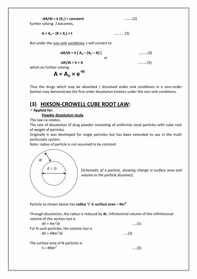
(3) HIXSON-CROWELL CUBE ROOT LAW: Applied for: Powder dissolution study This law co-relates, The rate of dissolution of drug powder consisting of uniformly sized particles with cube root of weight of particles. Originally it was developed for single particles but has been extended to use in the multi particulate system. Note: radius of particle is not assumed to be constant

[Schematic of a particle, showing change in surface area and volume as the particle dissolves].

Particle as shown above has radius ‘r’ & surface area = 4πr2 Through dissolution, the radius is reduced by dr, infinitesimal volume of this infinitesimal volume of this section lost is

dV = 4πr2dr …..(1) For N such particles, the volume loss is

dV = 4Nπr2dr …..(2) The surface area of N particles is

S = 4Nπr2 …..(3)

dr

d = 2r

Using Noyes-Whitney law; infinitesimal mass change will be: -dM = k × S × Cs × dt …..(4)

in which k is used for D/h Therefore , D / M = γ × dV (density (γ) = M/V) Therefore , -γ × dV = k × S × Cs × dt …..(5) Thus from (2), (3), (5),

-4Nπr2 × dr × γ = k × 4Nπr2 × Cs × dt …..(6)

dividing (6) by 4Nπr2 we get -γ × dr = k × Cs × dt …..(7) integrating with r = ro at time t = 0 (7) becomes r = ro – k × Cs × t /γ …..(8) for N particles: r = N × (ro – k × Cs × t /γ) for sphere, V = 4 × π r3 & V = M 3 γ Therefore, for N particles, M = 4 × π × N × (d /2)3 γ 3 So, M = π × N × γ × d3

6 …..(9) Where d = diameter of the sphere. Taking cube-root of (9) we get M1/3 = (N× γ × π/6)1/3 × d …..(10) Similarly Mo

1/3 = (N × γ × π/6)1/3 × do …..(11) Placing r = d/2 in eq.(8) d/2 = do/2 – k × Cs × t/γ …..(12) from eq. (9) & (10) placing the values of d and do eq. (12) becomes, 1 × ( M)1/3 1 × (Mo)1/3 – k × Cs × t 2 ( Nπγ/6)1/3 = 2 ( Nπγ/6)1/3 γ ……(13) further solving the eq.13 turns to be Mo

1/3 – M1/3 = 2 × k × Cs × (1 × N× π × γ)1/3 × t γ (6)1/3

taking 2 × k × Cs × 1 × N × π × γ)1/3 = K γ (6)1/3 eq. 13 becomes,

Mo1/3-M1/3 = K × t

where, Mo = original mass of A.P.I.particles

K = cube-root dissolution rate constant M = mass of the A.P.I at the time ‘t’ Equation 14 is called as Hixson Crowell Cube root law.

(4) TAKERU HIGUCHI MODEL:

Applied for the suspension type of ointment. The equation is derived for a system describe as follows:

a. Suspended drug is in a fine state such that the particles are much smaller in diameter than the thickness of applied layer

b. The amount of drug A, present per unit volume is substantially greater than the Cs, the solubility of the drug per unit volume of vehicle.

c. The surface to which drug ointment is applied is immiscible with respect to the ointment and consist of perfect sink for the released drug.

dh h

[Theoretical concentration profile existing in an ointment containing suspended drug and in contact with a perfect sink]. The solid line in the diagram represents the concentration gradient existing after time ‘t’ in ointment layer normal to the absorbing surface. The total drug concentration, as indicated in the drawing would be expected to show a more or less sharp discontinuity at distance ‘h’ from the surface, none of the suspended phase dissolving until the environmental concentration drops below Cs. Fick`s first law, dM = dQ = DCs Sdt dt h (1)

Static diffusion layer

Surrounding aq. Layer

Perfect sink

Matrix

Cs A

Reseding boundary Depleting zone

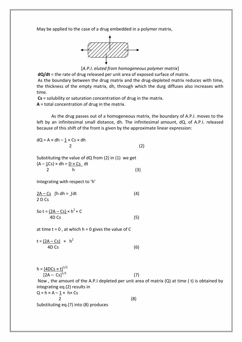
May be applied to the case of a drug embedded in a polymer matrix,

[A.P.I. eluted from homogeneous polymer matrix]

dQ/dt = the rate of drug released per unit area of exposed surface of matrix. As the boundary between the drug matrix and the drug-depleted matrix reduces with time, the thickness of the empty matrix, dh, through which the durg diffuses also increases with time. Cs = solubility or saturation concentration of drug in the matrix. A = total concentration of drug in the matrix. As the drug passes out of a homogeneous matrix, the boundary of A.P.I. moves to the left by an infinitesimal small distance, dh. The infinitesimal amount, dQ, of A.P.I. released because of this shift of the front is given by the approximate linear expression: dQ = A × dh – 1 × Cs × dh

2 (2) Substituting the value of dQ from (2) in (1) we get {A – 1Cs} × dh = D × Cs dt 2 h (3) Integrating with respect to ‘h’ 2A – Cs ∫h dh = ∫dt (4) 2 D Cs So t = (2A – Cs) × h2 + C 4D Cs (5) at time t = 0 , at which h = 0 gives the value of C t = (2A – Cs) × h2 4D Cs (6)

h = [4DCs × t]1/2 [2A – Cs]1/2 (7) Now , the amount of the A.P.I depleted per unit area of matrix (Q) at time ( t) is obtained by integrating eq.(2) results in Q = h × A – 1 × h× Cs 2 (8) Substituting eq.(7) into (8) produces

Q = {D × Cs × t}1/2(2A – Cs) {2A – Cs}1/2 (9) i.e.,

Q = [D (2A – Cs)Cs × t]1/2 (10) The above equation is known as Higuchi equation. Under normal conditions A >>Cs, and equation (10) reduces to

Q = (2A × D × Cs × t)1/2 (11) Thus for the release of a A.P.I. from a homogeneous polymer matrix-type delivery system, eq.(10) indicates that the amount of A.P.I. released is proportional to the square root of A = the total amount of A.P.I. in unit volume of matrix, D = the diffusion coefficient of the A.P.I. in the matrix Cs = the solubility of A.P.I. in polymeric matrix and t = time. Outcome of the Higuchi model :

The rate of release (dQ/dt) can be altered by increasing or decreasing A.P.I. solubility Cs in the polymer by complexation.

A= the total concentration of a A.P.I also influences the release rate.

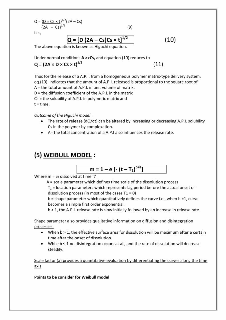
(5) WEIBULL MODEL :

m = 1 – e [- (t – T1)b/a] Where m = % dissolved at time ‘t’ A = scale parameter which defines time scale of the dissolution process

T1 = location parameters which represents lag period before the actual onset of dissolution process (in most of the cases T1 = 0) b = shape parameter which quantitatively defines the curve i.e., when b =1, curve becomes a simple first order exponential. b > 1, the A.P.I. release rate is slow initially followed by an increase in release rate.

Shape parameter also provides qualitative information on diffusion and disintegration processes.

When b > 1, the effective surface area for dissolution will be maximum after a certain time after the onset of dissolution.

While b ≤ 1 no disintegration occurs at all, and the rate of dissolution will decrease steadily.

Scale factor (a) provides a quantitative evaluation by differentiating the curves along the time axis Points to be consider for Weibull model

Success of this model depends on linearizing dissolution data. However a considerable curvature may be found in upper region of the plot if the accumulated fraction of A.P.I. dissolved is not 1.

In addition, location parameter, which represents the lag time before the actual onset of the dissolution process, has to be estimated indirectly by a least-square analysis or a graphical trial and error technique.

6.KORSEMEYAR AND PEPPAS MODEL : The KORSEMEYAR AND PEPPAS empirical expression relates the function of time for diffusion controlled mechanism. It is given by the equation: Mt/Ma = Ktn Log (Mt/Ma) = log K + n log t Where Mt / Ma is function of drug released t = time K=constant includes structural and geometrical characteristics of the dosage form n=release component which is indicative of drug release mechanism Where, n is diffusion exponent. If n is equal to 1 , the release is zero order . if the n = 0.5 the release is best described by the Fickian diffusion and if 0.5 < n < 1 then release is through anomalous diffusion or case two diffusion. In this model a plot of percent drug release versus time is liner. Inherent disadvantages of Model dependent approaches :

1) Violation of underlying statistical assumption 2) A model does not predict values with sufficient accuracy. Therefore statistical methods have been developed to determine the validity of underlying statistical assumption of models. Examples λ2 goodness of fit analysis is one of such method to evaluate validity of statistical

assumption of a model. Serial randomness of residuals,

Constancy of error variance, Normality of error terms. These all have been incorporated into computer programs.

MODEL INDEPENDENT METHODS It is mainly classified in to two major classes.

METHOD PARAMETER

Ratio of Percentage (%) Dissolved

Ratio of Area Under dissolution Curves (AUC)

Ratio Test Procedure

OR

Time Point Approach

Ratio of Mean Dissolution Time (MDT)

% Drug Release at Given Time ( Yx )

Time Require for Given % Release ( tz )

Pair wise Procedure

Index of Rescigno ( 1 and 2 )

Difference Factor (f1)

Similarity Factor (f2)

(A) Ratio Test Procedure

For particular sample time, each of the two formulations being compared and mean % dissolved and standard error (SE) are to be estimated. Standard Error of mean ratio (SET/R) can be determine by Delta method.

where, SET/R is the SE of the mean ratio of test to standard. XT is the mean percentage dissolved of test. XS is the mean percentage dissolved of standard.

Where, SET is the standard error of percentage dissolved for test. SER is the standard error of percentage dissolved for standard.

So, from mean ratio of the percentage dissolved and SET/R , a 90% confidence interval for

XT/XR is to be constructed. Similar procedure is followed for the ratio of Area Under the dissolution Curve (AUC)

and Mean Dissolution Time (MDT). AUC is calculated by Trapezoidal rule. MDT is calculated by following equation.

Where, i = dissolution sample number (e.g. i=1 for 5 min.,i=2 for 10 min. data)

n = total number of dissolution sample time. tmid = the time at mid point between i and i – 1

M = addition amount of drug dissolved between i and i –1

Time Point Approach In this approach either the percentage drug released at a given time ( e.g. Y60, Y300 or

Y480 ) or the time require for a given percentage of drug to be released ( e.g. t50%, t80% or t90% ) are often selected as responses.

Main application of this Time Point Approach is to distinguish good or bad batches where some specific dissolution parameters are predetermined. Disadvantages of Time Point Approach

Time Point Approach for the interpretation of dissolution data appears to be inadequate for complete characterization of the profile.

Consequently, the choice of single data points for the calculation of meaningful dissolution values is questionable, specially when it is related to bioequivalence procedure.

This approach is not much problematic in immediate release products but it has drastic effect with controlled release products.

(B) Pair Wise Procedure

DIFFERENCE FACTOR (f1) & SIMILARITY FACTOR (f2) These factors are introduced by MOORE AND FLANNER in 1996.

This approach is adopted by Center for Drug Evaluation and Research (CDER) of US-FDA and also by Human Medicine Evaluation Unit of European Agency for Evaluation of Medicinal Products (EMEA) as criteria for assessment of similarity between 2 dissolution profiles.

The difference factor (f1) as defined by FDA calculates the % difference between 2 curves at each time point and is a measurement of the relative error between 2 curves.

Where, n = number of time points

Rt = % dissolved at time t of reference product (pre change)

f1 =

n

t

n

t

Rt

TtRt

1

1 ×100

Tt = % dissolved at time t of test product (post change) The f1 equation is the sum of the absolute value of the vertical distance between the test and reference mean values, i.e. lRt-Ttl at each dissolution time point, expressed as percentage of sum of mean fraction released from reference formulation at each time point. The f1 equation is zero (0) when the mean profiles are identical and increases proportionally as the difference between the mean profile increase.

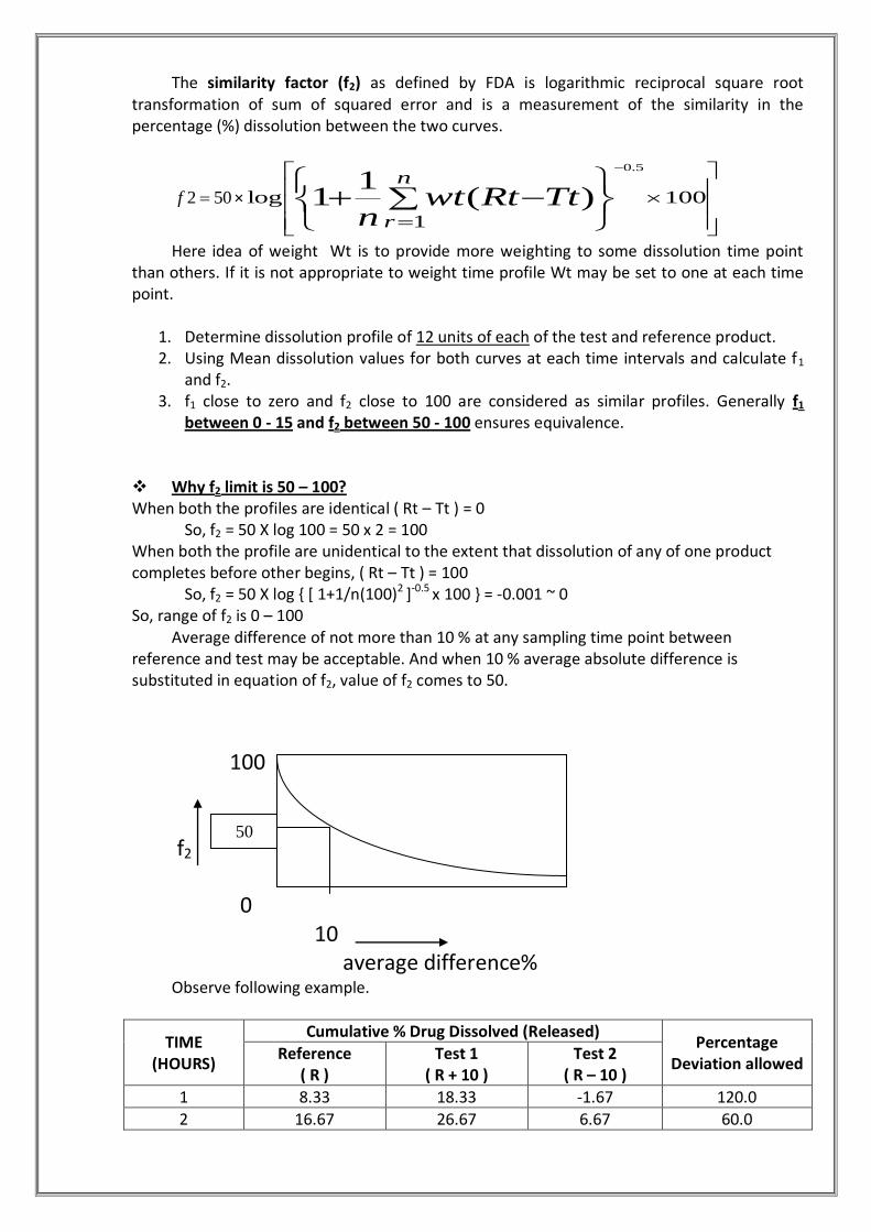
The similarity factor (f2) as defined by FDA is logarithmic reciprocal square root transformation of sum of squared error and is a measurement of the similarity in the percentage (%) dissolution between the two curves.

502 f ×

100

1

log )(1

1

5.0

n

r

TtRtwtn

Here idea of weight Wt is to provide more weighting to some dissolution time point than others. If it is not appropriate to weight time profile Wt may be set to one at each time point.

1. Determine dissolution profile of 12 units of each of the test and reference product. 2. Using Mean dissolution values for both curves at each time intervals and calculate f1

and f2. 3. f1 close to zero and f2 close to 100 are considered as similar profiles. Generally f1

between 0 - 15 and f2 between 50 - 100 ensures equivalence. Why f2 limit is 50 – 100? When both the profiles are identical ( Rt – Tt ) = 0

So, f2 = 50 X log 100 = 50 x 2 = 100 When both the profile are unidentical to the extent that dissolution of any of one product completes before other begins, ( Rt – Tt ) = 100 So, f2 = 50 X log { [ 1+1/n(100)2 ]-0.5 x 100 } = -0.001 ~ 0 So, range of f2 is 0 – 100

Average difference of not more than 10 % at any sampling time point between reference and test may be acceptable. And when 10 % average absolute difference is substituted in equation of f2, value of f2 comes to 50.

100 f2 0 10 average difference% Observe following example.

TIME (HOURS)

Cumulative % Drug Dissolved (Released) Percentage

Deviation allowed Reference

( R ) Test 1

( R + 10 ) Test 2

( R – 10 )

1 8.33 18.33 -1.67 120.0

2 16.67 26.67 6.67 60.0

50

3 25.00 35.00 15.00 40.0

4 33.33 43.33 53.33 30.0

5 41.67 51.67 31.67 24.0

6 50.00 60.00 40.00 20.0

7 58.33 68.33 48.33 17.1

8 66.67 76.67 56.67 15.0

9 75.00 85.00 65.00 13.3

10 83.33 93.33 73.33 12.0

11 91.67 101.67 81.67 10.9

12 100.00 110.00 90.00 10.0

For Reference Vs Test 1 f2 = 50 For Reference Vs Test 2 f2 = 50

Table 1. Calculation of Similarity Factor (f2)

So, finally acceptable limit defined as 50 – 100.

Recommendations to be taken in consideration 1. Dissolution measurement of both products made under exactly same conditions and

sample withdrawal timing should be also same. 2. Dissolution time points recommended for immediate release products are 15, 30, 45

and 60 minutes and for extended release products are 1, 2, 3, 5 and 8 hours. 3. f2 value is sensitive to the number of dissolution time points, so only one

measurement should be considered after 85 % dissolution of product. 4. For products which are rapidly dissolves, i.e. more than 85 % release in 15 minutes

or less, profile comparison is not necessary. 5. The mean dissolution value for Rf should be derived preferably from the last pre

changed (Reference) batch. 6. To allow the use of mean data, % coefficient of variation (% CV) at earlier time points

(e.g. 15 minutes ) should be not more than 20 % and at other time points should not more than 10 %.

Advantage (1) They are easy to compute (2) They provide a single number to describe the comparison of dissolution profile data.

Disadvantages (1) The f1 and f2 equations do not take into account the variability or correlation structure in the data. (2) The values of f1 and f2 are sensitive to the number of dissolution time point used. (3) If the test and reference formulation are inter changed , f2 is unchanged but f1 Is not yet differences between the two mean profile remain the same. The basis of the criteria for deciding the difference or similarity between dissolution profile is unclear.

Similarity factor (f2) is dependent on sampling scheme from apparatus means selection and determination of number of dissolution time points.

So that when we have same reference and test product, but if number and time of dissolution time points are different, they shows different results.

E.g. Viness Pillay et al had worked on High Density Sticking formulation of Theophylline and High Density System of Diltiazem HCL. In Theophylline,

When time points were taken up to 30.5 hours f2 was 49.85 and When time points were taken up to 35.0 hours f2 was 51.30.

In Diltiazem HCL, When time points were taken up to 15 hours f2 was 47.57 and

When time points were taken up to 25 hours f2 was 52.09 So, the variability is such that question arise, whether it is consider to be pass or fail ?

NOVEL APPROACHES

[1] Unbiased Similarity Factor f*2

In estimation of similarity factor f2 bias can occur due to contribution of the variance of the percentage drug dissolved measured at a particular time point. As such, unbiased similarity factor f *2 was calculated to determine the effect of time points of the test and reference on the f2. In this equation, subtraction of one term is done, where Sr and St Represents the variances of percentage drug dissolved measured at the nth time point and N is the number of the units of both products tested for dissolution.

[2] Lower acceptable value of f2 (f2LX) :

As we had seen previously about f2 limits, if the percentage drug release from reference is 15 at any time t, a range of 5 to 25 is permissible for the test product at same time. [See the % Deviation allowed in initial phase in table]. And this limit is very liberal especially when we consider about the sustain release formulation. In initial phase if sustain release product release 10 % more than what it should be then it causes the dose dumping, which should not be acceptable.

Another important point is, as we had seen in example in initial phase range is up to

negative value also, which is not practicable but even though if there is no drug release in initial phase it is acceptable as per current approach of f2 value.

So M.C.Gohel and M.K.Panchal had suggested the lower acceptance value where limit

is acceptable by deviation of X% of the actual % drug release for the same time point and not the absolute 10% drug release difference, where X is percentage deviation allowed like 2,5,10.

Here is the same example with 10% deviation allowed ( X = 10% ), where we can see easily how the acceptable range get narrowed.

TIME (HOURS)

Cumulative % Drug Dissolved (Released)

Reference ( R )

Test 1 ( R + 10% of R )

Test 2 ( R – 10 % of R)

1 8.33 9.17 7.50

2 16.67 18.33 15.00

3 25.00 27.50 22.50

4 33.33 36.67 30.00

5 41.67 45.83 37.50

6 50.00 55.00 45.00

7 58.33 64.17 52.50

8 66.67 73.33 60.00

9 75.00 82.50 67.50

10 83.33 91.97 75.00

11 91.67 100.83 82.50

12 100.00 110.00 90.00

For Reference Vs Test 1 f2LX = 60.33 For Reference Vs Test 2 f2LX = 60.33

Table 2. Calculation of Lower Acceptable Similarity Factor (f2LX)

MULTIVARIATE CONFIDENCE REGION PROCEDURE In the cases where within batch variation is more than 15% CV, a Multivariate model Independent procedure is more suitable for dissolution profile comparison.

It is also known as BOOT STRAP Approach. The following steps are suggested.

1. Determine the Similarity limits in terms of Multivariate Statistical Distance (MSD) based on interbatch differences in dissolution from reference (standard approved) batches.

2. Estimate the MSD between the test and reference mean dissolutions. 3. Estimate 90% confidence interval of true MSD between test and reference batches. 4. Compare the upper limit of the confidence interval with the similarity limit. The test

batch is considered similar to the reference batch if the upper limit of the confidence interval is less than or equal to the similarity limit.

INDEX OF RESCIGNO : - The Index of Rescigno was first introduced by Rescigno in 1992. Originally this method was developed to compare drug plasma concentration and time profiles. The general expression of Index of Rescigno {ξi(i=1,2)} for dissolution profile comparison may be written as follows:

Where, dR(t) and dT(t) are either the individual or mean percentage dissolved at each time point for the reference and test dissolution profiles respectively. Rt and Tt are the mean percentage dissolved for the reference and test formulation at each time point The indices can be thought of as a function of weighted average of vertical distance between test and reference mean profile at each time point. (Absolute value of the vertical distance in the case of ξ1 and square of the vertical distance in case of ξ2)

The denominator of ξi is a scaling factor. When i=1, ξ1 is area enclosed by test and

reference mean dissolution profile.

In practice, the indices ξi can be calculated by approximating the mean dissolution profile for

the reference and test formulation by straight line between each consecutive pair of time point. The indices lie between zero and one. The value of ξi close to zero indicates similarity between mean dissolution profiles. The value of ξi will be one if one of two mean dissolution profile is zero at each dissolution time point.

Here the main advantage over f1 and f2 value is, interchanging the test and reference data does not alter their value.

List of references:

1) www.dissolutiontechnology.com 2) Polli,Rekhi,Ausburger,Shah, J.Pharm.Sci.,86,6,690-700(1997) 3) www.fda.gov/cder/guidance.htm (dissolution testing of immediate release dosage

forms) 4) Modern Pharmaceutics, 3rd edition revised and expanded edited by G.S.Banker,

C.T.Rhodes 5) M.Gibaldi & S. Feidmon, J.Pharm.Sci.,56,10,1238-1242(1967) 6) Physical Pharmacy 4th edition Alfred Martin,333,335-336 7) T.Higuchi,J.Pharm.Sci,50,10,874-875(1961) 8) Viness Pillay & Reza Fassihi, J.Pharm.Sci.,88,9,849-850(1999) 9) Thomas O’Hara, Adian Dunna , Jackie Butler and John Devane ,pstt vol.1 , No.5 August

1998 page no.214-223