Competition for Order Flowand

Smart Order Routing Systems

Thierry FoucaultHEC School of Management, Paris, GREGHEC and CEPR

1 rue de la Liberation

78351 Jouy en Josas, France

e.mail : foucault@hec.fr

Albert J. MenkveldVrije Universiteit Amsterdam

De Boelelaan 1105

1081 HV Amsterdam, Netherlands

e.mail : ajmenkveld@feweb.vu.nl

November, 20051

1We thank Jean-François Gajewski, Oliver Hansch, Joel Hasbrouck, Terry Hendershott,Charles Jones, Stephen Mayhew, Christine Parlour, Ailsa Roëll, Gideon Saar, Chester Spatt,Patrik Sandås, Dan Weaver and seminar participants at Universitat Pompeu Fabra, the SEC,the NYSE, the University of Virginia, Paris XII, the International Conference on New FinancialMarket Structures in Montreal, the Workshop on Market Microstructure in Aix-en-Provence,the International Conference on Finance in Copenhagen, and the European Finance Association(EFA) Meeting in Moscow for useful comments. We also thank Patricia van Dam and Friso vanHuijstee for excellent research assistance. Last, we thank Euronext, the London Stock Exchangeand a Dutch online broker, Alex, for their sponsorship. Of course, we bear the entire responsibilityof the paper and all errors are ours.

Abstract

Competition for Order Flow and Smart Order Routing Systems

We study changes in liquidity following the introduction of a new electronic limit or-

der market when, prior to this introduction, trading is centralized in a single limit order

market. We also study how automation of routing decisions and trading fees affect the

relative liquidity of rival markets. The theoretical analysis yields two main predictions

: (i) other things equal, consolidated depth is larger in the multiple limit order markets

environment and (ii) other things equal, the liquidity of the entrant market relative to that

of the incumbent market increases with the level of automation for routing decisions (the

proportion of "smart routers"). We test these predictions by studying the rivalry between

the London Stock Exchange (the entrant market) and Euronext (the incumbent market)

in the Dutch stock market. The main predictions of the model are supported.

Keywords : Market Fragmentation, Centralized Limit Order Book, Smart Routers,Trading Fees, Trade-Throughs.

"When I was CEO of Tradepoint (now virt-X), my team and I spent a considerable

amount of effort ‘selling’ the exchange to traders. However, although they all signed up as

member, they did not use the market. One major reason was that access to the market

was not connected to their trading systems. Even when better bids and offers appeared on

our order book, the (momentarily) inferior prices available on the LSE were hit and lifted.

Potential users simply could not see, nor easily access the market. If the Tradepoint terminal

was at the end of the desk, it was not accessible." (in "Is exchange liquidity contestable?",

by Nic Stuchfield, The handbook of World Stock, Derivative and Commodity Exchange.)

1 Introduction

Automation has decreased the cost of developing trading systems, fostering the emergence

of new electronic marketplaces (e.g. ECNs, The International Securities Exchange, Trade-

point etc...) and competition for the order flow. The escalation of competition for order

flow implies that financial markets are ever more fragmented, both in the U.S. and in

Europe. Whether this evolution is desirable is highly controversial.1

In the U.S., for instance, it has fueled a debate over the benefits and costs of a central-

ized limit order book (CLOB), with strict price and time priority. Proponents of a CLOB

argue that it enhances liquidity and that it greatly facilitates the search for best execution.2

Opponents argue that multiple limit order markets, linked by smart order routing systems,

promote intermarket competition while retaining the benefits of order flow concentration,

as smart routing systems effectively consolidate offers in different markets (see Stoll (2001)

for a discussion).

One way to shed light on this debate consists in comparing measures of market liquidity

in two situations : (a) trading in a security is centralized in a single limit order book and

(b) trading in this security is fragmented across multiple and competing limit order books.

We perform this comparison, using an extension of the model of intermarket competition

developed by Parlour and Seppi (2003). We also test the predictions of our model, taking

advantage of a recent reorganization of the Dutch stock market. For long, trading in

this market has largely been centralized in a single limit order market, NSC, operated

by Euronext. This situation changed in May 2004 when the London Stock Exchange

1For an overview of the main issues, see "Request for Comment on Issues Relating to Market Fragmen-tation", (see SEC Release n◦34− 42450, available at http://www.sec.gov/rules/sro/nv9948n.html).

2In the U.S., institutions such as Morgan Stanley, Goldman Sachs and Merril Lynch have been promi-nent advocates of a CLOB. In contrast, ECNs have argued against. See “Don’t CLOBber ECNs”, WallStreet Journal, March 27, 2000 and “Sweeping Changes in Markets Sought”, Wall Street journal, February29, 2000.

1

introduced another electronic limit order market, EuroSETS, for stocks traded in NSC.

This introduction offers a unique opportunity to study empirically whether fragmentation

of liquidity among competing limit order books enhances or impairs liquidity.

The nature of our empirical analysis determines the directions in which we extend Par-

lour and Seppi (2003). Parlour and Seppi (2003) pit a pure limit order market against an

hybrid trading system (like the NYSE). In contrast, we focus our theoretical analysis on

competition between two pure limit order markets (an “incumbent” market and an “en-

trant” market) as NSC and EuroSETS are. Second, we allow competing markets to charge

different trading fees. In particular, consistent with the pricing strategy of EuroSETS

and many ECNs, we allow the entrant market to charge smaller fees on “passive” orders

(non-marketable limit orders) and larger fees on “aggressive” orders (marketable limit or-

ders). This is important because the fees charged in competing markets can determine the

outcome of intermarket competition. Third, we analyze how routing decisions affect this

outcome.

When a security trades in multiple markets, brokers face a search problem. The routing

decision is determined by a trade-off between the benefit of improved execution with the

cost of searching for improved execution (which includes the cost of checking offers in

various trading venues and the cost of splitting orders across these venues if beneficial). The

opening quotation suggests that even seemingly small search costs can result in violations

of price priority (“trade-throughs”) as brokers do not exert the effort of obtaining the

best possible price.3 This problem stifles intermarket competition as it reduces liquidity

providers’ incentives to post competitive prices. It is likely to be particularly acute for

entrant markets, like EuroSETS, because, by force of habit, brokers are naturally inclined

to check offers only in the incumbent market. Consequently, we assume that there are two

types of brokers : (i) smart routers, who systematically search for best execution and (ii)

non-smart routers, who exclusively trade in the incumbent market. We interpret smart

routers as brokers equipped with Smart Order Routing Systems (SORSs), a technology

that consolidate offers in different markets and route orders accordingly, so as to minimize

trading costs. More generally, they can be viewed as brokers with relatively small search

costs.

The model yields several testable predictions. First, consolidated depth at a certain

price (i.e. the total number of shares offered at that price or better in both markets) is

always larger in the multiple limit order markets environment. The absence of time priority

3Trade-throughs are well documented in U.S. markets. For instance, Battalio et al.(2004) find a sub-stantial proportion of trade-throughs in option markets. Trade-throughs also occur in equity markets(see Bessembinder (2003)), even though they are prohibited for markets participant to the ITS. See alsoHendershott and Jones (2005a).

2

across markets is key for this finding.4 Intuitively, it allows traders to jump in front of the

queue of limit orders placed at one price in, say, the incumbent market by submitting a

limit order at the same price in the entrant market. Queue-jumping competes away the

profits earned on inframarginal limit orders (those in front of the queue) in either market.

The reduction in liquidity providers’ rents translates in smaller trading costs (hence larger

consolidated depth), at the benefit of smart routers. This result holds whether the entrant

market charges smaller or larger fees than the incumbent market. However, a reduction

in fees on limit orders in either market (relative to the fees charged prior to the outset

of intermarket competition) amplifies the positive effect of intermarket competition on

consolidated depth. More generally, a reduction in fees on limit orders in one market

always triggers (i) an increase in the cumulative depth of this market and (ii) an increase

in consolidated depth.

Other things equal, the model implies that cumulative depth in the incumbent market

(i.e. the total number of shares offered up to a given price in this market) should be

smaller after introduction of the competing market. Actually, the entrant market diverts

part of the order flow. Consequently, the likelihood of execution for limit orders in the

incumbent market declines when the entrant market becomes active. If fees on limit orders

are unchanged, the expected revenue on a limit order in the incumbent market is smaller.

For this reason, in equilibrium, traders submit less limit orders in this market.5

Last, the model predicts a positive relationship between the competitiveness of the

entrant market and the fraction of trades conducted by smart routers (for short, "the pro-

portion of smart routers"). Intuitively, an increase in the proportion of smart routers raises

the execution probability of limit orders submitted to the entrant market. Accordingly,

traders are more willing to post competitive quotes in this market. Specifically, we find

that an increase in the proportion of smart routers enlarges (i) the fraction of total quoted

depth (the total number of shares offered at the best quotes) attributable to the entrant

market and (ii) the ratio of the inside spread in the incumbent market to the inside spread

in the entrant market.

We test these predictions using a sample of 22 stocks traded both in EuroSETS and

4In Parlour and Seppi (2003), intermarket competition can increase or decrease consolidated depth.The difference of result is due to the fact that one of the competing market has an hybrid market structurein their model.

5The absence of time priority is often viewed as deterring, instead of encouraging, liquidity provision(seeHarris (1990). In a sense the deterrence effect is present in our model : traders submit less limit orders inthe incumbent market because queue-jumping reduces the likelihood of execution in this market. However,queue-jumping facilitates "entry" of relatively slow bidders (those who submit orders at the end of thequeue). This second effect encourages competition between limit order traders and more than compensatesthe deterrence effect.

3

NSC. We consider 3 different sample periods : one sample period in May 2004, just before

the entry of EuroSETS and two sample periods (August 2004 and January 2005) after the

entry of EuroSETS. We group stocks in quartiles based on trading activity and we test

our predictions for each quartile, separately.

In order to analyze the effect of EuroSETS entry on consolidated depth, we build

snapshots of the consolidated limit order book (observed every 5 minutes) for each stock

and each sample period. We then compare consolidated depth before and after entry of

EuroSETS. After controlling for changes in market conditions in a multivariate setting, we

find that consolidated depth, throughout the book, is larger after entry. This increase is

significant for almost all quartiles and its magnitude is greater in the second post-entry

period. For instance, for the most actively traded stocks, we find that consolidated depth

at the fourth price behind the best quote has increased by 77% and 100.8% in the first

and second post entry periods, respectively. We also find that cumulative depth in NSC is

larger after the entry of EuroSETS, in both post-entry periods. We attribute this increase

in NSC cumulative depth to the reduction in its fees on limit orders around the time of

EuroSETS entry. The sharp increase in consolidated depth does not come at the cost of

larger inside spreads (the difference between the best ask price and the best bid price in the

consolidated limit order book). Actually, for both post-entry periods, we find that inside

spreads are smaller or unchanged relative to their pre-entry levels. We show theoretically

that this evolution is expected given the reduction in fees on limit orders following the

introduction of EuroSETS.

Next, we study the relationship between the proportion of smart routers and the liquid-

ity of EuroSETS relative to that of NSC (i.e. the fraction of total quoted depth attributable

to EuroSETS and the ratio of NSC bid-ask spread to EuroSETS bid-ask spread). In our

theoretical analysis, the likelihood of observing a buy (resp. sell) market order executed

in the entrant market, when this market is posting the best ask (resp. bid) price, is equal

to the proportion of smart routers. We exploit this observation to build a proxy for the

proportion of smart routers. We find that, on average, the proportion of smart routers is

small on average and that it does not increase over time (it is respectively equal to 27%

and 18% in each post-entry period).

As predicted by the model, we find a positive cross-sectional relationship between

EuroSETS competitiveness and the proportion of smart routers. In particular, EuroSETS’s

bid-ask spread relative to that of NSC is significantly smaller in stocks for which the

proportion of smart routers is large. Moreover, there is a positive relationship between

EuroSETS’s contribution to quoted depth and the proportion of smart routers (statistically

significant only in the second post-entry period). Importantly, these relationships are

4

robust when (i) we use alternative proxies for the proportion of smart routers (accounting

for more complex routing decisions for non-smart routers) and (ii) when we control for

other possible determinants of EuroSETS relative liquidity (in particular trading volume).

These findings suggest that there might be inertia in the adoption of SORS by brokerage

firms, a possibility consistent with the small proportion of smart routers in the case of

EuroSETS and NSC. Actually, the usefulness of a SORS for a given broker increases with

the liquidity of the entrant maket. But this liquidity depends positively on the adoption

decisions of other brokers. Therefore, the situation in which brokers decide not to adopt a

SORS because they expect little benefit from doing so is self-reinforcing.

There is a vast literature on market fragmentation (see Lee (2002) for a survey). The

theoretical literature usually concludes that fragmentation is harmful for liquidity (Mendel-

son (1987)) and traders’ welfare (Pagano (1989)). This literature, however, has not consid-

ered the effect of fragmentation on consolidated depth, as we do here. There also exist many

empirical studies on this topic.6 Most related to our paper are the studies that compare

measures of market liquidity before and after entry of new competitors in the provision

of trading services (e.g. Battalio (1997), Mayhew (2003), DeFontnouvelle et al. (2003),

Boehmer and Boehmer (2004), Battalio et al.(2004), Biais, Bisière and Spatt (2004)). In

general, these studies find that spreads are tighter after entry, which show that intermar-

ket competition is an important complement to intramarket competition. However, to the

best of our knowledge, there are no empirical evidences regarding competition between

pure limit order markets.7

Glosten (1994) analyzes theoretically competition between pure limit order markets.8

He shows that consolidated depth is identical when order flow concentrates in a single

market or fragments between several limit order markets (see Proposition 8 in Glosten

(1994)). In this model, limit order traders get zero expected profits because (i) there is

free-entry of limit order traders and (ii) a pro-rata allocation rule is used when several limit

order traders post the same price. Introduction of a new limit order market is therefore

redundant. Glosten (1998) shows that this prediction does not hold if time priority is

used instead of a pro-rata allocation rule.9 When time priority is enforced within a limit

6For instance, Hamilton (1979), Bessembinder (2003), Barclay et al. (2003), Fink et al. (2004),Hendershott and Jones (2005b).

7Board and Wells (2000) study competition between SETS and Tradepoint (2 UK based limit ordermarkets). They do not study the effect of this competition on consolidated depth, however.

8Some authors study competition between a pure limit order market and a market using a differenttrading mechanism, e.g. a dealership market (as in Viswanathan and Wang (2002) or Sabourin (2004)) oran hybrid market (as in Parlour and Seppi (2003)). Other papers on competition between markets (e.g.Pagano (1989), Chowdry and Nanda (1991) or Hendershott and Mendelson (2000)) do not consider limitorder markets.

9Biais, Martimort and Rochet (2000) relax the free-entry assumption. They show that liquidity sup-

5

order book, infra-marginal limit orders get strictly positive expected profits. In this case,

introduction of a new limit order market allows traders to compete away these expected

profits if time priority is not enforced across markets. As a result, consolidated depth

can be larger in the multiple markets environment. Our framework is very different from

Glosten (1998) (e.g. there is no asymmetric information in our setting) but, interestingly,

a similar economic intuition explains why intermarket competition enhances consolidated

depth.

The plan of the paper is as follows. We describe the model Section 2. Section 3 derives

the main implications of the model. Section 4 describes the natural experiment conducted

in this paper and reports the empirical findings. Section 5 concludes. All the proofs are in

the Appendix.

2 Competition for Order Flow with Smart Routers.

2.1 Model

As explained in the introduction, the model builds upon Parlour and Seppi (2003). There

are 3 periods in this model. In period 1, limit order traders post offers in the competing

markets. In period 2, a broker arrives. She must execute immediately an order for eXshares on behalf of a client. In period 3, payoffs are realized. We now explain in more

details the trading rules and the actions available to the traders intervening in periods 1

and 2.

Competing Markets.

There are two markets : (a) the incumbent market, denoted I and (b) the entrant

market, denoted E. A risky security, with expected final payoff v0, trades on these two

markets. Both markets are organized as limit order markets. In each market, traders

position their limit orders on a price grid. The tick size, i.e. the difference between two

successive prices on the grid, (pi+1 − pi), is equal to ∆. Last, we set p0def= v0.

From now on, we exclusively focus on the determination of the number of shares offered

on the “ask side” of the book (that is at prices {p1, p2...}).10 It is straightforward to derive

pliers earn strictly positive expected profits when their number is finite. These profits decrease and themarket becomes deeper as the number of liquidity suppliers increases.10In this model, it is never optimal to submit a sell (resp. buy) limit order below (resp. above) v0 (see

below).

6

symmetric results for the “bid side” of the book. We denote by Sjk the number of shares

offered for sale at price pk (k ≥ 1) in market j. The cumulative depth at price pk in marketj is denoted by Qjk (with Qj0 = 0). We denote by Qk the consolidated depth at price pk,

that is the total number of shares offered up to price pk in Markets I and E. Formally :

Qjk = Qjk−1 + Sjk, ∀k ≥ 1 (1)

and

Qk = QIk +QEk, ∀k ≥ 1. (2)

Price and time priority are enforced within each market but not across markets. When

a buy (resp. sell) market order is routed to market j, it executes against the limit orders

standing in this market at progressively higher (resp. lower) prices until completion of the

order. Moreover, limit orders standing at a given price are filled in the sequence in which

they were submitted (time priority).

Limit Order Traders.

Limit orders in each market are submitted by risk-neutral traders who arrive at sto-

chastic point in times during period 1. The trader who arrives first in Market j ∈ {I,E}sees an empty book and fills the book. Then a new trader arrives, observes the book, and

decides to add depth to the book or not. The process stops when there is no price in each

book at which submitting a limit order is profitable.11 Then, the trading game proceeds

to period 2.

Limit order traders active in Market j bear two distinct costs. First, they bear an

execution cost fj ≥ 0, per share, when their order executes in market j. This cost includesthe execution fee charged by Market j and other order-handling costs (back-office, clearing

and settlement costs etc...). Second, they bear an order entry cost cj > 0 per share,

whether their order is executed or not. This cost includes the entry fee charged by Market

j but also the costs associated with the time required to submit and then monitor the

order. Importantly, this cost is paid whether execution takes place or not, in contrast to

the execution fee, fj. We interpret differences in order entry costs or execution costs across

markets as resulting from differences in the fees charged by each market (as order-handling

costs and monitoring costs are likely to be identical across markets).12 In this paper, we

11As in Parlour and Seppi (1997), we assume that the number of potential liquidity suppliers is infinite.12Some markets do charge order entry fees (e.g. Euronext). But this practice is not common. However,

it is worth stressing that cj does not need to be a fee paid to Market j as this parameter absorbs anycost borne by a trader who submits a limit order. The model encompasses the particular case in whichcI = cE . For our empirical analysis, the relevant case is cI > cE as EuroSETS does not charge order entryfees while NSC does (see Section 4).

7

take execution and entry costs as given and we analyze the optimal reaction of market

participants to these costs.

Market Orders and Smart Routers.

The broker arriving in period 2 must fill a market order on behalf of a client. A client

is characterized by (a) the size of his order, eX, (b) the direction of his order (buy/sell)and (c) his reservation price. We assume that the client is a buyer with probability α and

that eX, is random with a cumulative probability distribution F (.). The client’s reservationprice is fixed and equal to pm > p1. Thus, the broker never executes a market order at a

price strictly larger than pm.13 For this reason, limit orders at prices strictly larger than

pm have a zero execution probability and are never submitted.

The broker has one of two types : (i) either she is a smart router (probability γ) or

(ii) she is not (probability (1 − γ)). In the latter case, she only considers the incumbent

market as a possible trading venue. In contrast, a smart router consolidates offers in both

trading systems and optimally splits her order between markets I and E so as to minimize

total trading cost. If the broker’s order size is x > Qm then she executes all limit orders

placed at prices p1,p2, ..., pm in each market. The residual portion is left unexecuted. If the

broker’s order size is x ∈ [Qs−1, Qs] with s ≤ m then she executes all limit orders placed

at prices p1,p2, ..., ps in each market.

In general, at the stop-out price ps, there are several ways to allocate the residual

portion, (x−Qk−1), of the market order between the two competing markets. We assume

that smart routers use one of two tie-breaking rules in this case : (a) trade first in market I

and then execute the residual (if any) in market E or (b) trade first in E and then in I. A

proportion δI (resp. δE = 1− δI) of smart routers uses the first (resp. second) tie-breaking

rule. For the moment, we assume that markets I and E charge no fees on market orders.

In Section 4.2. we relax this assumption and show that δI should be determined by the

fees on market orders.

We interpret smart routers as traders equipped with Smart Order Routing Systems

(SORSs). For these traders, the cost of searching for the best routing strategy and imple-

menting it is nil as the search process is completely automated. However, smart routers

can be viewed more generally as brokers who systematically search for the smallest trading

costs. In contrast, we view non-smart routers as brokers who handle orders manually.

In order to economize on search costs, they trade only in one market.14 In Section 4.2,

13This assumption is innocuous as our results do not depend on pm. It just guarantees that a buy orderdoes not get executed at an infinite price because the limit order book is too thin to absorb the entireorder.14The quotation opening the present article suggests that the mere fact of switching terminals to check

8

we show how to extend the model when non-smart routers use a more complex routing

strategy.

Strictly speaking, parameter γ is the proportion of trades intermediated by smart

routers. For brevity, we refer to this parameter as being "the proportion of smart routers".

Two polar cases are of special interest. Consider the case γ = 0, first. In this case, brokers

exclusively trade in the incumbent market. Obviously, this case is similar to the situation

in which the incumbent market operates alone. We can therefore develop predictions about

the effects of introducing a new trading venue by comparing liquidity when (i) γ = 0 and

(ii) γ > 0. The case γ = 1 constitutes another interesting situation. In this case, brokers

can costlessly use both systems and thereby orders freely flow to the cheapest market.

This case occurs when all brokers are smart routers. Alternatively, it represents a situ-

ation in which trade-throughs (i.e. violations of price priority) are prohibited or avoided

by adequate intermarket linkages. For instance, in the U.S., markets participating to ITS

(Intermarket Trading System) agreements for stocks listed on the NYSE must either (a)

match the intermarket best offer (resp. best bid price ) or (b) reroute market buy (resp.

sell) orders to the market posting the best offer (resp. bid price) when the order arrives.15

2.2 The Competitive Equilibrium

We focus on competitive equilibria, i.e. situations such that limit order books posted at

the end of period 1 leave no profit opportunities. In this section, we define these equilibria

formally.

Let PIk(QIk−1, Qk−1, SIk, SEk) and PEk(Qk−1, SIk, SEk) be the probabilities that all

shares offered at price pk in markets I and E, respectively, get executed. As time pri-

ority is enforced within each market, execution of all shares offered at price pk in Market j

is equivalent to execution of the last share offered at price pk in Market j (“the marginal

limit order” at this price). For this reason, we refer to Pjk as being the execution probability

of the marginal order at price pk in Market j. The next lemma relates the Pjks0 to the

probability distribution of the market order size. We denote the likelihood that a market

order is larger than x by F (x)def= 1− F (x).

offers in the entrant market might be perceived as being "too costly" ( "Potential users simply couldnot see, nor easily access the market. If the Tradepoint terminal was at the end of the desk, it was notaccessible [...]").15There is no trade-through regulation in the market considered in our empirical analysis. Moreover,

in this market, best execution is defined with respect to a benchmark, which is the price posted in the“main” market (i.e. NSC), rather than the best price across all trading venues. Thus, brokers might indeedchoose to avoid searching for the best price. Indeed, as shown in Section 4, we find frequent occurences oftrade-throughs in our empirical analysis.

9

Lemma 1 : The execution probabilities of the marginal order placed at price pk ≤ pm in

the incumbent and the entrant markets are, respectively:

PIk(QIk−1, Qk−1, SIk, SEk) = α[(1−γ)F (QIk−1+SIk)+γ(δIF (Qk−1+SIk)+δEF (Qk−1+SIk+SEk))]

(3)

and

PEk(Qk−1, SIk, SEk) = αγ[δEF (Qk−1 + SEk) + δIF (Qk−1 + SIk + SEk)] (4)

For a given state of the limit order book in each market, consider a trader who adds

a limit order for an infinitesimal number of shares at price pk in Market j. As the order

is at the end of the queue of limit orders submitted at price pk in Market j, its execution

probability is Pjk. The trader’s expected profit is equal to his revenue in case of execution

times the execution probability minus the order entry cost. Thus, if the trader operates in

Market I, his expected profit (per share) is :

ΠmIk(QIk−1, Qk−1, SIk, SEk) = PIk(QIk−1, Qk−1, SIk, SEk)(pk − v0 − fI)− cI (5)

Similarly, if the trader operates in market E, his expected profit is:

ΠmEk(Qk−1, SIk, SEk) = PEk(Qk−1, SIk, SEk)(pk − v0 − fE)− cE. (6)

Other things equal, the execution probability of the marginal order at a given price is

decreasing with the number of shares (Sjk) offered at this price (see Equations (3) and

(4)). Hence, as the number of shares offered at price pk in Market j increases, the expected

profit on the marginal order at this price decreases and is eventually zero. At this point,

no trader finds optimal to add depth at price pk in market j. If this zero profit condition

holds at each price in the book, there are no profit opportunities left in Market j and,

in this sense, a competitive equilibrium is reached (see Seppi (1997), Sandås (2001) and

Parlour and Seppi (2003)). Let Q∗k(γ), Q∗jk(γ), S

∗jk(γ) denote the equilibrium values of

the consolidated, cumulative and quoted depths at price pk. Formally, a competitive

equilibrium is defined as follows (see Definition 2 in Parlour and Seppi (2003)).

Definition 1 : A competitive equilibrium is a set of depths {S∗Ik, S∗Ek}k=mk=1 such that the

expected profit of the marginal limit order at each price pk in each limit order book is

non-positive if S∗jk = 0 and nil if S∗jk > 0. Formally, for k ∈ [1,m] :

ΠmIk(Q

∗Ik−1, Q

∗k−1, S

∗Ik, S

∗Ek) = 0 if S

∗Ik > 0 and Πm

Ik(Q∗Ik−1, Q

∗k−1, S

∗Ik, S

∗Ek) ≤ 0 if S∗Ik = 0,

ΠmEk(Q

∗k−1, S

∗Ik, S

∗Ek) = 0 if S

∗Ek > 0 and Πm

Ek(Q∗k−1, S

∗Ik, S

∗Ek) ≤ 0 if S∗Ek = 0.

10

It is worth emphasizing two features of competitive equilibria, as they play an important

role in the rest of the analysis.

1. Limit orders at the end of the queue at a given price just break-even. But infra-

marginal orders get strictly positive expected profits (e.g. ΠmIk(Q

∗Ik−1, Q

∗k−1, SIk, S

∗Ek) >

0 if 0 < SIk < S∗Ik). Ultimately, this explains why, in this model, the incumbent mar-

ket is not “competition-proof” if time priority is not enforced across markets.

2. A limit order book can feature prices at which no limit order are submitted (S∗jk = 0).

This happens when the execution probability at a given price price is small so that

a limit order at this price is not profitable. If, for a given market, there are no prices

at which submitting a limit order is profitable then the book in this market is empty

and the market is not viable.

The last remark implies that there are two possible equilibrium outcomes : either (i)

each market attracts some limit orders or (ii) one market does not attract any limit order.

In the first case, the execution probability of the limit orders standing in each book must be

strictly positive, which means that trades will occur in both markets. Hence, we say that

the two markets coexist when the books in each market are non-empty in equilibrium. In

the second case, obviously, trading concentrates in the market where limit orders cluster.

We say that this market is the dominant market.

Definition 2 : Market j is dominant if the book of the competing market is empty for allpossible reservation prices, that is : S∗−jk(γ) = 0,∀k, ∀m. Otherwise, Markets E and Icoexist.

Let bcj def=

cjαand Rjk

def=

cj(pk−v0−fj) . Using Equations (5), (6) and the equilibrium

definition, it is immediate that a competitive equilibrium is reached when the S∗jk(γ)s’

solve the following system of 2m equations :

PIk(Q∗Ik−1, Q

∗k−1, S

∗Ik, S

∗Ek) = RIk if S∗Ik > 0, k ∈ {1, ...,m}, (7)

PIk(Q∗Ik−1, Q

∗k−1, S

∗Ik, S

∗Ek) ≤ RIk or RIk ≤ 0 if S∗Ik = 0, k ∈ {1, ...,m},

PEk(Q∗k−1, S

∗Ik, S

∗Ek) = REk if S∗Ek > 0, k ∈ {1, ...,m}, (8)

PEk(Q∗k−1, S

∗Ik, S

∗Ek) ≤ REk or RIk ≤ 0 if S∗Ek = 0, k ∈ {1, ...,m},

11

For fixed values of parameters γ and δI , the equilibrium S∗jks’ are completely determined

by the Rjks’. An increase in the order entry cost (cj) or in the order execution cost (fj)

triggers an increase in Rjk. Thus, qualitatively, an increase in the order execution cost

in Market j has the same effect on the equilibrium as an increase in the order entry cost

in this market. In order to simplify the exposition, we can therefore normalize fI and

fE to zero. We have checked that all our results are robust when 0 < fj. In particular,

qualitatively, our statements regarding the effect of order entry costs also apply to order

execution costs on limit orders.

For some values of the parameters and an adequate specification of F (.), it is possible

to solve the previous system of equations and obtain closed-form solutions for cumulative

depths and consolidated depth. However, our implications (derived in the next section) do

not rely on a specific parametrization of the model. They just follow from the equilibrium

conditions (7) and (8).

Benchmark: When market I operates alone (γ = 0), the expected profit on the

marginal limit order at price pk in market I is :

ΠmIk = α[F (QIk−1 + SIk)(pk − v0)− bcI ] = α[F (QIk)(pk − v0)− bcI ] for k ≤ m.

Recall that Q∗Ik(0) denote the cumulative depth posted at price pk in equilibrium when

γ = 0. In a competitive equilibrium, it is such that the expected profit on the marginal

limit order at price pk is equal to zero, i.e. :

F (Q∗Ik(0))(pk − v0)− bcI = 0 for k ≤ m. (9)

Observe that F (x) decreases with x and is bounded by 1. Thus, if (pk − v0) < bcI , thereis no solution to this equation and Q∗Ik(0) = 0. The first price on the grid at which

some sell limit orders are submitted (the best offer price) is the smallest price a∗ such that

(a∗ − v0)− bcI > 0. To fix things, we assume that :A.1 bcI < p1 − v0, (10)

so that a∗ = p1. This assumption is not crucial for the results. It simply fixes the size of

the inside spread in the consolidated market to 1 tick. Under this assumption, Q∗Ik(0) > 0,

∀k ≥ 1 and Q∗Ik(0) increases with k. Below, we study whether the consolidated depth

when the entrant market is active is larger or smaller than when Market I operates alone.

12

3 The effects of intermarket competition

3.1 Is Market Fragmentation Harmful for Market Liquidity?

We first study the conditions under which Markets I and E coexist or not (Propositions 1

and 2). The next proposition shows that Market E is viable if and only if the proportion

of smart routers exceeds a critical mass.

Proposition 1 (critical mass): Let γ∗(bcE,bcI , δI) def= Min{ cE(2−δI)cI ,

cEδIcI+(1−δI)∆}. If γ ≤ γ∗

(bcE,bcI , δI) then Market I is dominant in equilibrium. If γ∗ (bcE,bcI , δI) < γ < 1 then both

markets coexist.

This result underscores the importance of routing systems for the entrant. The latter

is able to steer away some orders from the entrant market iff the proportion of smart

routers is larger than a critical mass, equal to γ∗ (bcE,bcI , δI).16 The intuition for this resultis simple. Other things equal, the likelihood of execution for limit orders placed in the

entrant market increases with the proportion of smart routers. When the proportion of

smart routers is small, the expected revenue from submitting a limit order in the entrant

market is too small to cover the entry cost in this market, at any price. As a result, no

limit orders are submitted in the entrant market.

If γ∗ (bcE,bcI , δI) < γ < 1, the two markets coexist. The situation in which γ = 1

deserves a special treatment because the incumbent market has no captive base of users

in this case. Yet, as shown in the next proposition, the two markets can charge different

entry fees and coexist in this case as well. Let bc∗E def= Min{ cI

1+δI, cI−δI∆1−δI }.

Proposition 2 :Suppose that all traders are smart routers (γ = 1) and that γ∗ < 1. IfbcE > bc∗E then both markets coexist. If bcE ≤ bc∗E then market E is dominant.Using the conditions derived in Propositions 1 and 2, Figure 1 depicts the set of values

for γ and bcE such that (a) market I dominates or (b) the two markets coexist (for fixedvalues of bcI and δI).17

16This can explain why the LSE has repeatedly encouraged brokerage firms to develop Smart OrderRouting Systems since the introduction of EuroSETS. For instance, it organized meetings between Dutchbrokerage firms and developers of SORSs. On the day following the introduction of EuroSETS, the FT waswriting, "The London Stock Exchange which yesterday started an assault on Amsterdam stock is drawingattention to traders’ increasing need for smart order routeing to take advantage of increased competition"("LSE tries the smart order route", Financial Times, May 25 2004).17The conditions include the polar cases in which δI = 1 or δE = 1. These polar cases are discussed in

more details in Corollary 1 below.

13

[insert Figure 1]

Even when γ = 1, the two markets coexist for a wide range of parameter values (bc∗E <bcE < (2− δI)bcI if bcI > ∆2), including cases in which the two markets charge different order

entry fees. That is, trading does not necessarily concentrate in the market charging the

lowest fee. This means that routing decisions for limit orders are not infinitely elastic to

order entry fees. Why?

Limit order traders’ placement decision is determined by a trade-off between execution

probability and order entry cost. Submitting a limit order to the market with the largest

order entry fee can be optimal if the execution probability in this market is larger than

in the competing market. To see this point, consider the case in which the incumbent

market charges larger fees (bcE < bcI). Initially, when books are empty, limit order tradersshould choose the entrant market. But, as the queue of limit orders in the entrant market

becomes larger, the execution probability of a limit order in this market diminishes while

the execution probability of the first limit order submitted in the incumbent market remains

high. For a sufficiently large queue in the entrant market, the benefit of a relatively high

execution probability in the incumbent market counterbalances the benefit of a relatively

small order entry fee in the entrant market, if bcE > bc∗E. It is then optimal to start fillingthe book in the incumbent market.

For instance, suppose that SE1 shares are offered at price p1 in market E while no limit

orders are posted in market I, yet. Moreover, assume that all traders are smart routers.

Then, consider a trader submitting a limit order for an infinitesimal quantity at price p1in market E. His execution probability is (see Equation (4)):

PE1(0, 0, SE1) = αF (SE1). (11)

If, instead, the trader submits his order in Market I, he obtains an execution probability

equal to (see Equation (3)):

PI1(0, 0, 0, SE1) = α(δIF (0)+ δEF (SE1)) = α(δI +(1− δI)F (SE1)) ≥ PE1(0, 0, SE1). (12)

Hence, the trader gets a larger execution probability if he places his limit order in the

incumbent market. On balance, placing a limit order in the incumbent market is optimal

if :

PI1(0, 0, 0, SE1)(p1 − v0)− cI > PE1(0, 0, SE1)(p1 − v0)− cE,

14

which yields (using Equations (11) and (12)):

δI(1− F (SE1))∆ > (bcI − bcE). (13)

Clearly, even if bcI > bcE, placing a limit order in the incumbent market becomes optimalwhen the queue of limit orders at price p1 in the entrant market, SE1, is large enough (for

δI > 0).

This reasoning crucially depends on the fact that time priority is not enforced across

markets. To see this, re-consider the argument when time priority is enforced across

markets. The limit orders standing at price p1 in Market E have time precedence. Thus,

a new limit order submitted at price p1 has the same execution probability, αF (SE1),

whether the order is submitted in Market E or Market I. Clearly, in this case, limit orders

should always be directed to the market charging the smallest entry fee. In contrast, when

time priority is not enforced across markets, submitting a limit order in one market is

in effect a way to jump in front of the queue of limit orders placed at the same price in

the competing market.18 Traders are willing to pay for this possibility as it raises their

execution probability and, in this way, the two markets can coexist even if they charge

different fees on limit orders.

We now analyze the effect of intermarket competition on the cumulative depth of

the incumbent market. Before entry, the marginal limit order at price pk just breaks-even

when the cumulative depth at this price is Q∗k(0). If the cumulative depth in the incumbent

market is unchanged after entry, the execution probability of the marginal limit order at

price pk in this market is necessarily smaller as part of the order flow executes against the

entrant limit order book. In these conditions, the marginal limit order at price pk in the

incumbent market loses money. Thus, the cumulative depth at price pk must be reduced

after entry of market E, as shown in the next proposition.

Proposition 3 : Other things equal, when the two markets coexist or when Market E isdominant, the cumulative market depth in the incumbent market is smaller than when the

incumbent market operates alone. This means that :

Q∗Ik(γ) ≤ Q∗k(0) ∀k ≥ 1 when γ ∈ [γ∗, 1].18Anedoctal evidences suggest that limit order traders do use queue-jumping strategies in presence of

multiple trading venues. For instance, the August 2004 issue of the EuroSETS newsletter mentions that:"[...] some firms are using the relatively lower volumes on the spread offered by the Dutch Trading Serviceto "queue-jump" rather than waiting elsewhere for execution" (EuroSETS newsletter, Issue August 2004,4).

15

Now we consider the effect of intermarket competition on consolidated depth. Suppose

that the books in the incumbent and the entrant markets have filled in such a way that

consolidated depth at price pk is smaller than or equal to its level when the incumbent

market operates alone (i.e. Qk ≤ Q∗k(0)). This situation cannot constitute an equilibrium

because profit opportunities remain, at least in the incumbent market. Actually, the

marginal limit order in the incumbent market yields time priority only to the limit orders

offered in this market, not to all the limit orders in the consolidated market. Thus, its

execution probability is larger than if offers were consolidated in a single market with time

priority enforced. Formally, this follows from Equation (3), which yields

αF (Qk) < PIk(QIk−1, Qk−1, SIk, SEk), (14)

since Qk−1+SIk < Qk (if both markets coexist, there are some limit orders posted at price

pk in both markets). The expected profit on the marginal limit order in the incumbent

market is then strictly larger than if offers were consolidated in a single market with time

priority enforced. Accordingly, the level of consolidated depth for which no further profit

opportunities would remain in the centralized market (i.e. Q∗k(0)) leaves room for profit op-

portunities in the fragmented market. Thus, consolidated depth in the fragmented market

must be larger than when a single market operates, as claimed in the next proposition.

Proposition 4 :When the two markets coexist (i.e. γ > γ∗ and cE > c∗E), consolidated

market depth is larger than when the incumbent market operates alone, i.e. Q∗k(γ) ≥ Q∗k(0),

∀k ≥ 1. Specifically, there exists k0 such that :

Q∗k(γ) > Q∗k(0), ∀k ≥ k0,

and

Q∗k(γ) = Q∗k(0), ∀k < k0.

It is worth stressing that this result obtains even if order entry costs are larger in the

entrant market.19 Key to this finding is the absence of time priority across markets, not the

pricing policy of the entrant market. This absence enables traders to bypass time priority

on limit orders standing at a given price in one market by submitting a limit order at the

same price in the competing market. We call this effect of intermarket competition, the

“queue-jumping effect”. It intensifies competition among limit order traders. Accordingly,

19The results only depend on the fact that the two markets coexist, not on the fees. However, for δI = 1,the two markets coexist only if cE < cI . Thus, in this polar case, Proposition 4 indirectly requires a smallerfee in the entrant market. Moreover, the value of k0 depends on the fees. For instance, it can be shownthat k0 decreases as cE becomes smaller.

16

rents on inframarginal limit orders in either markets are reduced and overall trading costs

for smart routers are reduced (i.e. consolidated depth increaes).

Intermarket competition is likely to prompt a reduction in the fees charged on passive

orders. The next proposition analyzes the effect of a reduction in these fees on consolidated

depth.We focus on a reduction in order entry costs as execution fees have been normalized

to zero. However, the same result obtain if we consider variations in execution fees instead

of variations in order entry costs. See the remark following Equations (7) and (8).

Proposition 5 : If Market j is viable (i.e. if it coexists with its competitor or dominatesthe market) then a reduction in the order entry cost of Market j results in an increase in

cumulative depth in Market j and an increase in consolidated depth.

To understand this result, suppose that the incumbent market reduces its fees on passive

orders. Cumulative depth in the incumbent market increases as providing liquidity in

this market becomes less expensive. Accordingly, the likelihood of execution for limit

orders placed in the entrant market becomes smaller. Limit order trading in this market

is less attractive and it becomes thinner. However, consolidated depth increases as the

increase in cumulative depth in the incumbent market more than compensates the decline

in cumulative depth of the entrant market.

This proposition implies that a reduction in order entry fees is a second channel through

which intermarket competition can enhance consolidated depth. To see this, consider

a scenario in which the entrant market charges a smaller order entry fee than the fee

charged by the incumbent market prior to entry (this is indeed the case in the experiment

considered in the empirical analysis). The previous propositions imply that the increase in

consolidated depth following the introduction of a new trading platform can be due both

to (i) the queue-jumping effect and (ii) a price war between competing platforms. The

following example illustrates this point, which is important for the interpretation of the

empirical findings.

Example : Suppose that γ = 1, δI = δE = 0.5 and that eX has a uniform distribution

on [0, Q]. Let bcbI and bcaI be the order entry costs in the incumbent market before and afterentry (bcaI ≤ bcbI < ∆). In this case, if caI−δI∆

1−δI < bcE <∆+caI2, then the equilibrium is such that

there are limit orders posted in each market at price p1. In this case, the quoted depths in

17

the incumbent market and the entrant market are respectively :20

Q∗I1(1) =2Q

3(1− 2bcaI − bcE

∆),

and

Q∗E1(1) =2Q

3(1− 2bcE − bcaI

∆),

In contrast, when the incumbent market operates alone, the quoted depth is :f

Q∗I1(0) = Q(1− bcbI∆),

In this case, the change in consolidated depth at price p1 is :

Q∗I1(1) +Q∗E1(1)−Q∗I1(0) = Q[∆− bcbI3∆

] + 2Q[bcbI − bcE3∆

] + 2Q[bcbI − bcaI3∆

]

Suppose first that fees on passive orders are identical before and after entry (bcE = bcaI = bcbI).The increase in quoted depth is then given by the first term in bracket in the previous

equation. It is due to the possibility of using queue-jumping strategies when the two

markets coexist. Now, suppose that the entrant market charges a strictly smaller fee on

passive orders than the pre-entry fee (bcE < bcbI). This triggers an additional increase inquoted depth given by the second term in bracket. Last, if the incumbent market reduces

its fee on passive orders after entry of the new competitor, consolidated depth increases

by an additional amount given by the last term in bracket in the previous equation. This

example illustrates (for the depth at the top of the book only) the two mechanisms (queue-

jumping and reduction in fees on passive orders) by which intermarket competition can

trigger an increase in consolidated depth.¥

We have not yet discussed the evolution of consolidated depth when, after entry, the

entrant market is dominant. Observe that Market E is dominant if and only if bcE ≤Min{ cI

1+δI, cI−δI∆1−δI } (Proposition 2). Thus, bcE ≤ bcI when the entrant market is dominant

(with a strict inequality when δI > 0). The equilibrium in this case is identical to the

equilibrium in the benchmark case but with a smaller fee on passive orders. The next

proposition immediately follows.

Proposition 6 : If the entrant market dominates then consolidated depth is larger thanwhen the incumbent market operates alone.

20Given the parametric assumptions, it is straightforward to derive the quoted depth in each marketusing Equations (7) and (8). The condition caI−δI∆

1−δI < bcE <∆+caI2 guarantees that Qj1(0) > 0 for each

market.

18

In summary, we find that, other things equal, consolidated depth is larger when multiple

limit order markets compete for order flow compared to a situation in which the order flow

is centralized in a single limit order book. Moreover, a reduction in the fees charged

on passive orders further increase consolidated depth. Thus, the average markup (resp.

discount) paid by smart routers on buy (resp. sell) orders is smaller when the two markets

coexist.

3.2 Extensions

Raw vs. Net Prices. In the baseline model, we have assumed that execution costson market orders were zero. In reality, traders also pay execution fees on market orders,

which can be different from execution fees on limit orders. In this case, the routing decision

should be determined by net prices (prices including execution fees) instead of raw prices,

i.e. displayed quotes.21 The model can easily be generalized to account for execution fees

on market orders. Let Φjb be the fee, per share, charged on market orders executed in

market j by broker b and suppose, to simplify the exposition, that 0 ≤ Φjb < ∆. We allow

the execution fee to vary across brokerage firms for more generality. The next lemma gives

the optimal routing strategy for smart routers given their execution fee on market orders.

Lemma 2 : Consider a smart router who must execute an order with size x ∈ [Qs−1, Qs].

If Φjb < Φ−jb then she optimally executes all limit orders placed at prices p1, p2, ..., ps−1 in

markets E and I. At the stop-out price ps, she gives priority to market j.

This result is straightforward. For instance, suppose that ΦIb < ΦEb. Observe that

pk + ΦEb < pk+1 as ΦEb < ∆. Thus, the quote montage in terms of net prices ranks the

offers standing in markets E and I in the following order: (i) Q1I shares at p1 + ΦIb, (ii)

Q1E shares at p1 + ΦEb, (iii) Q2I shares at p2 + ΦIb, (iv) Q2E shares at p2 + ΦEb etc... It

is then immediate that the routing strategy described in the previous lemma is optimal.

We deduce that δI is equal to the proportion of brokerage firms for which ΦIb < ΦEb. The

results of the previous sections are still valid as they have been derived for all possible

values of δI .

The fees structure. The previous remark suggests to interpret δj as resulting (atleast in part) from the fees charged on aggressive orders by Market j. Thus, we can

interpret variations in cj (or fj) or δj as being due to variations in the fees chosen by

21There are practical difficulties in building quote montages based on net prices (in particular becauseexecution fees can vary across investors). In reality, it is unclear whether routing decisions are made onthe basis of net or raw prices (see McCleskey (2004), Chapter 7 on this point).

19

market j. For instance, the effect of a decrease in fees on passive (resp. aggressive) orders

in market j can be analyzed in this model by studying the effect of a decrease in cj (resp.

δj ).

The fees affects the critical mass of smart routers, γ∗, required for the viability of

the entrant market. Using the expression for γ∗, it is immediate that the critical mass

decreases with bcI , increases with bcE and increases with δI . Hence, charging relatively smallfees can be a way for the entrant market to reduce the critical mass required to attract

some trading activity. Conversely, reducing its fees is a way for the incumbent market to

predate entry of a new competitor.

Competing markets often choose to charge different fees on passive orders and on ag-

gressive orders. This results in a situation in which one market appears more competitive

(in terms of fees) for one type of order (e.g. passive orders) and less for the other type (e.g.

aggressive orders). This is indeed the fees structure adopted by ECNs (e.g. Inet) or the

LSE for EuroSETS.22 The next corollary suggests that asymetries in the fees structures

between competing markets facilitate their coexistence. In this corollary, index j refers to

one market (I or E) and index "−j" to the competing market (i.e. if j = I then −j = E).

Corollary 1 : If γ = 1 and δj = 1 then the two markets coexist if cj > c−j >cj2. If

cj < c−j then trading concentrates in Market j. If c−j ≤ cj2then trading concentrates in

Market −j.

This corollary derives directly from Propositions 1 and 2 in the special case in which

δj = 1. It shows that even in this polar case, the two markets can coexist. This happens

if the market that has no priority in case of a tie (δ−j = 0) is more competitive on passive

orders (c−j < cj). Otherwise, trading concentrates in the market with the smallest fees.

In this paper, we take the fees charged by each market as given. An interesting extension

would be to endogenize these fees. The previous corollary suggests that competing markets

might prefer an outcome with differentiated fees structures as it allows both competitors

to be active. In contrast, entering into a price war on both passive and aggressive orders

results in a situation in which trading concentrates in a single market (so that there is

room for only one market). A full analysis of this question is beyond the scope of the

current article, however.

Varying Search Costs. In the baseline model, we have focused on a situation in whichthe population of brokers is divided into two distinct categories : (i) smart routers and (ii)

22For instance, Inet offers a rebate of $0.002 per executed share on limit orders adding liquidity to itsbook and charges a fee of $0.003 per executed share on orders removing liquidity from its book.

20

non-smart routers. For a given order size, smart routers only base their routing decisions

on the quotes available in each system and split their orders so as to minimize trading

costs. In contrast, non-smart routers ignore the prices available in the entrant market.

One possible explanation is that the cost of searching for best execution is very large for

these traders. In reality, non smart routers’ incentives to search for best execution might

vary with market conditions. In particular, these incentives are smaller in fast moving

markets because (i) the quotes standing in either market change quickly compared to the

time needed to split orders and (ii) the opportunity cost of time is larger. In contrast,

in slow markets, brokers are likely to be more patient and to consider the quotes in both

trading venues to execute their orders.

This possibility however does not change the results of the model. To see this point,

assume that a broker searches for best execution if her search cost, eCb, is smaller than a

threshold eTbt. This threshold can be a function, for instance, of market conditions (e.g.trading activity, volatility) and trade size.23 In this case, the likelihood that, on a given

order t, a broker behaves as a smart router is :

γt = γ + (1− γ) Pr(0 < eCb ≤ eTbt),as γ is the proportion of brokers who systematically search for best execution. The results

of the model are unchanged (simply γt plays the role of γ in all equations). In particular,

our results regarding changes in the proportion of γ, remain valid as γt is increasing in γ.

3.3 Empirical Implications

Now, we derive testable predictions of the model. These predictions are tested in the next

section by studying the rivalry between two pure limit order markets, EuroSETS (London

Stock Exchange) and NSC (Euronext). As explained below, this rivalry offers an ideal

laboratory to test our predictions because it approximates well the nature of competition

in our theoretical model. Moreover, EuroSETS was introduced after NSC, which gives us

the opportunity to compare measures of market liquidity before and after introduction of

EuroSETS.

Implications for market depth. Proposition 4 yields the most basic prediction.Namely, we should observe an increase in consolidated depth before and after the intro-

duction of EuroSETS, other things equal. As explained in the next section, fees on passive

23A full analysis of the determinants of this threshold requires to model the search process of brokersnot equipped with a SORS. This is beyond the scope of this paper.

21

orders are unambiguously smaller after EuroSETS introduction. According to the model,

this should amplify the increase in consolidated depth due to the queue-jumping effect (see

the discussion following Proposition 5).

Other things equal, the cumulative depth in NSC should decline after the introduction of

EuroSETS (Proposition 3). However, the fees on passive orders have been reduced in NSC

a few weeks before the entry of EuroSETS. This reduction should contribute to an increase

in NSC cumulative depth (Proposition 5). Moreover, if traders react to this reduction with

delay, we might see an increase in NSC cumulative depth after entry. Actually, on the one

hand, intermarket competition works to reduce NSC cumulative depth but on the other

hand the reduction in NSC fees works to increase cumulative depth in NSC. The second

effect can dominate if the reduction in fees on passive orders is large enough.

Let C1E(γ)def=

Q∗E1(γ)Q∗1(γ)

be the ratio of the cumulative depth in the entrant market at the

best ask price (i.e. p1) to the consolidated depth offered at this price for a given value of γ.

This ratio measures the contribution of the entrant market to the total number of shares

offered at the best ask price.

Proposition 7 : Other things equal, when the two markets coexist, the contribution of theentrant market to the consolidated depth at price p1 increases with the proportion of smart

routers (i.e. ∂C1E(γ)∂γ

> 0).

The intuition is simple. An increase in the proportion of smart routers enlarges the

execution probability of the marginal limit order submitted at the best ask (resp. bid)

price in the entrant market. Thus, it raises the expected profits on limit orders submitted

at this price in the entrant market. As a result, the quoted depth of the entrant market

(i.e. Q∗E1(γ)) increases. This indirectly decreases the execution probability of the marginal

limit order placed at the best ask (resp. bid) price in the incumbent market and thereby

it reduces the quoted depth in this market (Q∗I1(γ)). Eventually, the fraction of quoted

depth in the consolidated market attributable to the entrant market enlarges. In order to

test this prediction, we need to estimate the proportion of smart routers, γ. In Section 5,

we propose a methodology to estimate this parameter from the order routing choices that

we observe.

Implications for bid-ask spreads. First, we consider the effect of a change in theproportion of smart routers on the relative positions of the best ask (resp. bid) price in each

market. Depending on the values of γ, the best ask price in the incumbent market can be

strictly smaller, equal to or strictly larger than the best ask price in the entrant market, as

shown by the next proposition. Let γ∗∗def= cE

δIcI+(1−δI)∆and γ∗∗∗def= Min{1, ∆−cI+(1−δI)cE

(1−δI)∆ }.It is easily shown that γ∗∗ < γ∗∗∗.

22

Proposition 8 :

1. When γ∗ < γ ≤ γ∗∗, the two markets coexist and the best ask price in the entrant

market is strictly larger than the best ask price in the incumbent market. The interval

(γ∗, γ∗∗] is non-empty if and only if bcI > ∆2.

2. When Max{γ∗,γ∗∗} < γ < γ∗∗∗, the two markets coexist and the best ask price in the

incumbent market is identical to the best ask price in the entrant market.

3. When γ∗∗∗ < γ < 1, the two markets coexist and the best ask price in the incumbent

market is strictly larger than the best ask price in the entrant market. The interval

[γ∗∗∗, 1] is non-empty if and only if bcE < cI−δI∆1−δI .

When γ∗ < γ ≤ γ∗∗, a sell limit order placed at price p1 in the entrant market cannot

break-even because its execution probability is too small. However, it is profitable to submit

sell limit orders at larger prices. Thus, the two markets coexist but the ask price posted

in the incumbent market is strictly smaller than in the entrant market. The symmetric

situation occurs when γ∗∗∗ < γ < 1. Thus, for given order entry fees and for a fixed value

of δI , the model predicts an inverse relationship between the frequency with which the

incumbent market is not active at the best quotes and the proportion of smart routers,

i.e. γ. This implies that the ratio of the inside spread in the incumbent market to the

inside spread in the entrant market should be positively related to the proportion of smart

routers.

Now, we turn our attention to the effect of intermarket competition on the bid-ask

spread in the consolidated market (i.e. the difference between the best offer and the best bid

price in the consolidated market). As we focus only on the sell side of the book, we measure

the bid-ask spread in the consolidated market by the difference between the smallest ask

price at which shares are offered and v0. Under Assumption A.1, this difference is always

equal to 1 tick whether the two markets coexist or not. However, when Assumption A.1

is relaxed, we obtain the following result.

Proposition 9 : Suppose that prior to the introduction of market E, the order entry costin the incumbent market is such that bcI > ∆ (i.e. A.1 does not hold). If, after entry of

market E, the order entry cost for limit orders are unchanged or smaller in at least one of

the two markets then the bid-ask spread in the consolidated market is unchanged or smaller

compared to its pre-entry level.

The intuition is straightfoward. The smallest offer at which providing liquidity is prof-

itable enlarges with the order submission cost in this model. Thus, a reduction in this cost,

23

either leaves unchanged the bid-ask spread or reduces it (if the reduction in submission

cost is large enough). More generally, the proposition implies that a reduction in fees

on passive orders translates in a decrease in bid-ask spreads. As we already pointed out,

these fees have decreased after the introduction of EuroSETS. Thus, according to the last

proposition, we expect the bid-ask spread in the consolidated market to stay put or to

decrease following the introduction of EuroSETS.

To sum up, the model generates three clear-cut predictions : (i) consolidated depth

should be larger after entry of EuroSETS; (ii) the bid-ask spread in the consolidated

market should be unchanged or smaller after entry of EuroSETS and (iii) the liquidity

of EuroSETS relative to the liquidity of NSC (measured by the fraction of quoted depth

attributable to EuroSETS and by the ratio of NSC bid-ask spread to EuroSETS bid-ask

spread) is positively related to the proportion of smart routers. We test these predictions

in the next section.

4 Empirical Analysis

In this section, we test the predictions derived in Section 4.3 in the context of the rivalry

between the London Stock Exchange and Euronext in the Dutch equity market Section

5.1 provides a detailed account of this rivalry. Section 5.2 describes the dataset. The

remaining sections present the empirical findings.

4.1 Background and Data

4.1.1 Market Structures and Fees.

On October, 14, 2003, the London Stock Exchange announced that it would introduce a

new trading platform, EuroSETS, for the 48 stocks constituents of the two major Dutch

indices, the AMX and AEX. This introduction was encouraged by the Dutch brokerage

community, as a way to prompt the incumbent market, Euronext, to cut its trading fees.24

Euronext operates the main electronic trading platform for Dutch stocks, NSC, since the

merger of the Amsterdam and the Paris bourse in 2001. Trading in EuroSETS began on

May, 24 2004.

The differentiation between EuroSETS and NSC is minimal for 3 reasons. First, these

24See “Discontented Dutch Brokers prompt Foreign Intervention”, Euromoney, December 2003 or“Dutch Auction; Can the LSE snatch Dutch equities trading from Euronext?”, The Economist, 3/6/04.

24

two trading systems use very similar trading rules. They operate over the same trading

hours (9:00 am to 5:30 p.m.) and they are both organized as continuous, electronic, limit

order markets (see Biais, Hillion and Spatt (1995) for a detailed description of standard

trading rules in these markets). As both systems are automated, they offer the same speed

of execution. They have the same amount of transparency : (i) participants can see all

limit orders standing in each book (except hidden orders) and (ii) trading is completely

anonymous in each market. Also, EuroSETS and NSC use the same tick size, 0.01 euros,

for stocks with prices below 50 euros. Moreover, time and price priority are enforced within

each market (but not across the two systems). Second, the members of both markets are

almost identical as most brokerage firms have signed up to be a member of EuroSETS.25

Last, the two trading systems use the same clearing and settlement system, Clearnet. Thus,

in deciding where to trade, brokers should mainly trade-off (i) prices in both systems, (ii)

trading fees and (iii) search costs, assumed in our model.

Fees on passive orders are smaller after the introduction of EuroSETS, for two reasons.

First, the fees charged on passive orders in EuroSETS are smaller than those charged

in NSC before and after entry. In fact EuroSETS charges no order entry fee and offers

rebates in case of execution on passive orders. Second, Euronext has reduced its fees on

passive orders several times since the LSE announced its plan to enter the Dutch market.

These fees were reduced a first time by 50% on April, 23, 2004. Then, a few days before

the introduction of EuroSETS, Euronext launched the “European Soccer Championship”

summer special, running from May, 24 to July 31, 2004. During this period, rebates were

offered for passive orders submitted to NSC and aggressive orders were free of order entry

fees.

EuroSETS charges smaller fees than NSC on passive orders but not necessarily on

aggressive orders. As an illustration, consider a broker submitting less than 60,000 orders

per month.26 Based on documents released by Euronext and the LSE, we estimate the fees

for this broker as follows.

Passive Order Aggressive Order(€) Entry Execution Entry ExecutionFee Structure NSC 0.15 0.665 0.30 0.665/trade

EuroSETS 0.00 -0.02/€1,000 0.00 0.08/€1,000

Suppose that the broker submits a median size order for 1,500 shares at €15. If the25In its December 2004 newsletter, the LSE lists the 53 brokerage firms that use the service. It includes

all major brokers e.g. ABN AMRO, RABO, Van Der Moolen, Goldman Sachs, Merrill Lynch, and MorganStanley.26An exact comparison of the fees charged by EuroSETS and NSC is difficult as charges per order can

vary according to several factors specific to each broker (e.g. its monthly total trading volume with a givenmarket).

25

order is passive, EuroSETS is cheaper (zero entry fee in EuroSETS plus a rebate in case of

execution). If the order is aggressive, NSC is cheaper as the order is charged €0.965 (€0.30

entry plus €0.665 execution) on NSC and €1.80 on EuroSETS (0.08*1.5*15). Thus, we

expect δI to be close to 1 in the experiment considered in our empirical analysis.

Overall, the nature of competition between EuroSETS and NSC fits well the assumption

of our model as (i) both markets are pure electronic limit order markets with similar rules,

and (ii) the routing decision should mainly be driven by fees, prices and search costs as both

systems have almost identical membership and the same clearing and settlement system.

Thus, the introduction of EuroSETS creates an ideal laboratory to test the predictions of

the theoretical model.

4.1.2 Data

We compare measures of market liquidity before and after the entry of EuroSETS. To

this end, we select a pre-entry period and two post-entry periods of 21 trading days. The

pre-entry period starts on April, 23 and lasts until May, 21, 2004. In order to better

identify permanent equilibrium effects of EuroSETS entry, we consider two distinct post-

entry periods. The first post-entry period runs from August 2 through August 30, 2004.

The second post-entry period covers January 3 through January 31, 2005.

Observe that our pre and post-entry periods are chosen in such way that the fee struc-

ture of Euronext is in principle fixed over all periods. Actually, the pre-entry period starts

on the date at which Euronext announced and implemented its new fee structure whereas

the post-entry periods do not include the “summer specials” (May, 24 to July, 30). Hence,

we expect the cumulative depth in NSC to decrease if the impact of the initial reduction in

fees on Euronext is fully reflected into NSC cumulative depth on April 23, 2004. If instead,

the cumulative depth in NSC slowly adjusts to the new fees then we can observe either an

increase or a decrease in NSC cumulative depth (see the discussion in Section 3.3). In any

case, the fees on passive orders are smaller than those charged in the pre-entry period. This

implies that an increase in consolidated depth can be due to both (i) the queue-jumping

effect and (ii) the reduction in order entry fees for liquidity providers (see Proposition 5

and its discussion).

Our sample includes stocks constituents of the AEX index (25 stocks). In order to

avoid confounding effects, we remove (i) stocks with a price larger than 50 euros (because

they trade with a different tick size in each market), (ii) stocks that drop from or enter

in the index during the sample period or (iii) stocks that implement or cancel an ADR

program during the sample periods. This leads us to remove 3 stocks, Unilever, Gucci

26

and Numico from our sample. We group the remaining 22 stocks in quartiles based on

trading volume, with Q1 containing the most traded stocks. The classification is based on

2003 volume to ensure an exogenous ranking. The composition of the quartiles is given in

Appendix B. Stocks in the first quartile accounts for 66% of total volume and 71% of total

market capitalization.

We use two types of data in our analysis: (i) five-minute order book snapshots and (ii)

continuous time data on trades and best bid and ask quotes. The snapshot data contain

the five best bid and ask quotes and the number of shares offered at these quotes sampled

every five minutes, in both EuroSETS and NSC. We use these data to build snapshots

of consolidated limit order books every 5 minutes. The continuous time data consists of

time-stamped (to the nearest second) trades for both markets, best bid and ask quotes for

NSC, and best bid and ask quotes (including depth) for EuroSETS.27

Our data have some limitations. First, we do not have data on trades occuring in

other trading venues for the stocks in our sample. There are 3 main alternative possible

venues : (i) an OTC market, which plays the role of an upstairs market for the stocks in

our sample, (ii) “Xetra star”, a trading platform operated by Deutsche Börse (introduced

in 2003) and (iii) foreign markets for cross-listed stocks. The market share of Xetra star

is very small. Half of the stocks in our sample have ADRs’ listed in the US. The order

flow for these stocks is likely to be channeled by US brokerage firms. This is important as

these firms are used to trade in a more fragmented environment (the US equity market).

Thus, they are more likely to be equipped with a smart routing technology or at least to

behave like smart routers.28 This fact may explain generate cross-sectional variations in

the proportion of trades routed by smart routers (see below).

A second limitation is that both EuroSETS and NSC allow traders to use iceberg

orders. Iceberg orders are such that only a fraction of the entire order is disclosed to market

participants. We do not have data on these orders. Thus, we can measure the change in

displayed consolidated depth following EuroSETS entry, not the change in overall (hidden

and displayed) consolidated depth. The change in displayed depth can underestimate the

change in total depth if hidden depth has increased and /or hidden depth in EuroSETS

is large. Alternatively, the change in displayed depth can overestimate the change in

total depth if hidden depth in NSC has decreased. We have no ways to discard the first

possibility. We address empirically the second problem by analyzing the evolution of

27The continuous time data are regular “TAQ” data from Euronext and the LSE. The EuroSETSsnapshots, were made available to us by the LSE. The NSC snapshots were downloaded (with permissionof Euronext and the data provider) from a Dutch retail broker, Alex, who offers a live feed to the Euronexttrading platform.28Hallam and Idelson (2003) compare the usage of smart routing technologies in Europe and in the US.

They show that SORSs are more frequently used in the US.

27

effective spreads in NSC (see below).

4.2 Depth, Bid-Ask Spreads and Market Fragmentation

4.2.1 Methodology and Summary Statistics.

Most of our analysis in this section consists in comparing quartile means for various mar-

ket variables (e.g. the depth in the consolidated market) before and after the entry of

EuroSETS. We estimate these quartile means, changes in these quartile means and test

for the statistical significance of these changes using panel data techniques.

The general methodology is as follows. Let q ∈ {1, 2, 3, 4} be a quartile index andDPost−Entry be a dummy variable equal to 1 after entry of EuroSETS. We estimate the

following equation :

yit =Xq

µqDq +Xq

δqDPost−Entryq +

Xi

βixit + εit (15)

εit =Xi

ζiDi +Xt

ξtDt + ηit (16)

where yit is the dependent variable for stock i on day t (e.g. the daily average quoted spread

in the consolidated market for a given stock), µq is a quartile-specific mean, xit is a set of

control variables, ζi is a stock fixed-effect and ξt is a fixed time-effect.29 We estimate both

effects through the inclusion of dummies (Dis’ and Dts’). We are particularly interested

in δq, which measures the impact of EuroSETS entry on the dependent variable, for each

quartile. For the estimation, we exclude the dummy for the first stock in a quartile to

prevent collinearity. The dummies for the other stocks take value -1 for the first stock

to ensure that µq estimates the quartile-mean (instead of the first stock mean in the

quartile). We proceed in the same way for the time dummy. Following Petersen (2005),

our t-statistics are based on Rogers standard errors to account for non-zero (stock-specific)

autocorrelation in the error term (ηit).30

[insert Table 1]

Table 1 provides summary statistics on daily volume, daily number of trades, daily

average trade size, daily realized volatility (based on 5 minutes mid-quotes returns) and29We prefer fixed to random effects, as we do not, ex ante, want to rule out that our control variables

are correlated with the effect (see e.g. Greene (2002)).30Roger standard errors are similar in spirit to Newey-West standard errors, but are designed for panel

data analysis. The main difference is in the weights of the cross-terms. See Petersen (2005) for details.

28

average price level. It also provides EuroSETS and NSC market shares (in terms of trading

volume and number of trades) for each quartile. The first column reports the average values

for these variables in the pre-entry period for each quartile. It testifies to the heterogenous

nature of the sample. For instance, the average daily trading volume ranges from €167.33

million for Q1 to €9.4 million for Q4. Realized volatility (annualized) is 35.25% for Q4

and declines to 19.13% for Q1. We observe a significant drop in trading activity (-13% for

trading volume) and volatility (-7%) in the first post-entry period. In contrast, trading

activity is not significantly different in the second post-entry period, compared to the pre-

entry period. Volatility remains significantly lower (-36%). We will control for changes

in volatility, volume and price levels by including these variables as control variables in

Equation (15).

On average, EuroSETS’s daily market share in terms of total number of trades is 3.2%

(resp. 2%) in the first (resp. second) post-entry period. For stocks in Q1, EuroSETS’s

market shares in terms of number of trades are 6% (resp. 3.7%) in the first (resp. sec-

ond) post-entry period. For other stocks, the market share is less than 1%. Results are

roughly similar for market shares in terms of trading volume. As a point of comparison,

Bessembinder (2003) finds that the market shares of regional exchanges in terms of trading

volume for NYSE listed common stocks ranges from 2.18% (Philadelphia Stock Exchange)

to 8.21% (Chicago Stock Exchange). Thus, for stocks in Q1, EuroSETS’s market share

seems comparable to the market share of the most active regional exchanges in the U.S.

4.2.2 The Impact of Entry on Consolidated Depth.

We study the effect of EuroSETS introduction on measures of market liquidity, namely (i)

the relative quoted spread (i.e. the bid-ask spread in euros divided by price level), and

(ii) the total number of shares offered up to k ticks behind the best quotes, both in the

consolidated limit order book and in NSC limit order book. To save space, we just report

the findings for k = 0 (depth at the best quotes) and k = 4, as the conclusions are identical

across all values of k (for k ∈ {0, . . . , 4}). Also, for depth, we just report the results for theask side of the book. The results for the bid side are similar. Our main prediction is that

consolidated depth is larger after EuroSETS entry throughout the book (i.e. for all values

of k). As for the quoted bid-ask spread in the consolidated market, it should be either

unchanged or smaller, since fees on passive orders are smaller in the post-entry periods.

[insert Table 2 about here]

[insert Table 3 about here]

29

Table 2 contains the univariate results. It gives the average level of each liquidity mea-

sure in (a) the consolidated market and (b) NSC, before and after entry of EuroSETS. It

also reports the level of these liquidity measures for EuroSETS. Table 3 reports the esti-

mates for the coefficients in Equation (15) with (i) our measures of liquidity as dependent

variables and (ii) volume, volatility and price level as control variables. The conclusions

that emerge from the univariate and the multivariate analysis are similar. Thus, we focus

our discussion on the findings in Table 3. The coefficient of interest is δq, which measures,

for a given quartile, the impact of EuroSETS introduction on liquidity, after controlling

for other variables affecting liquidity.

Consolidated depth. Consolidated depth is larger after EuroSETS entry throughoutthe limit order book, for all quartiles. In economic terms, the increase in consolidated

depth is particularly impressive when compared to pre-entry levels (reported in Table 2).

For stocks in Q1, we find that quoted depth (Depth0) in the consolidated market increased

by 46.3% in the first post-entry period and 100.8% in the second post entry period. For

stocks in Q2, the percentage increases in quoted depth are respectively 48.1% and 97.8%.

For stocks in Q3 and Q4, we also find increases in excess of 30%. However, for these stocks,

the improvement in quoted depth relative to its pre-entry level is smaller in the second

post-entry period.

In the first post-entry period, changes in consolidated depth are in general statistically

significant throughout the book for all quartiles (except for the quoted depth in Q3). These

changes remain highly significant in the second post-entry period for stocks in Q1 and Q2

but not for stocks in Q3 and Q4.

Cumulative Depth in NSC. In general, the pattern for the evolution of cumulativedepth in NSC is similar to the pattern described for the evolution of consolidated depth.

First, the change in cumulative depth is positive throughout the limit order book for all

quartiles and for both post-entry periods. Second, in economic terms, the increase is

substantial. For instance for stocks in Q1, quoted depth in NSC increases by 24.8% in the

first post-entry period and 74.4% in the second post entry period. In this case as well, the

increase in depth is much larger for stocks in Q1. Third, the change in NSC cumulative

depth is statistically significant for almost all quartiles in the first post-entry period and

significant only for stocks in Q1 and Q2 in the second post-entry period.

At first glance, the increase in NSC cumulative depth is not consistent with the model

as the fee structure of NSC is unchanged across all the sample periods in our experiment.

In this case, Proposition 3 predicts a decline in depth for the incumbent market, not an

increase. However, recall that our pre-entry period starts on the date on which NSC

announced its cut in fees (April, 23 2004). The logic of the model implies that NSC

30

cumulative depth should increase on this date. In reality, cumulative depth might not

adjust to its new equilibrium level instantaneously. If the adjustment takes time then we

will observe a positive drift in the evolution of cumulative depth in NSC. The data are

consistent with this scenario.

Another possible explanation is that limit order traders in NSC have substituted iceberg

orders with fully displayed orders after the introduction of NSC. Then, total depth in NSC

might be unchanged or smaller after EuroSETS introduction, even though displayed depth

has increased. If this is the case, price impact of market orders executed in NSC should

be unchanged or larger in the post-entry periods. In order to study this question, we

compute the effective spread in NSC. The effective spread is twice the amount by which

the average (volume-weighted) execution price of a buy (resp. sell) market order exceeds

(resp. is below) the contemporaneous midquote in NSC. For all stocks in our sample, we

find (see Table 2) that the average effective spread in NSC is significantly smaller in the

second post-entry period compared to the pre-entry period. For the first post-entry, we

find no significant change in average effective spreads across all stocks in our sample. A

more detailed analysis for each quartile reveals that the magnitude and the direction of

the changes in average effective spreads closely match the changes in quoted spreads in

NSC (discussed below). Thus, overall, changes in effective spreads do not indicate that

NSC hidden depth has decreased.

Quoted Spreads. After entry of EuroSETS, the quoted spread in the consolidatedmarket (i.e. the difference between the best offer and the best bid across the two trading

venues) is smaller for all quartiles in the second post-event period. This is also the case for

the stocks in Q1 and Q2 in the first post-event period but not for the stocks in Q3 and Q4.

However, the increase in the quoted spread for these stocks is not statistically significant.

In all cases, the change in quoted spreads appears small in economic terms. For instance,

consider stocks in Q1. The average price level for these stocks before entry is €21.22 and

the average relative quoted spread is equal to 7.91 basis points. Thus, the average quoted

spread is equal to 1.6 cents before entry, slightly more than 1 tick. In the first post-entry

period, the decline in the quoted spread is equal to 1.16 basis points, less than 0.2 cents.

This is small, both relative to the pre-entry bid-ask spread and the tick size.

The findings are similar for the quoted spread in NSC. In general, the quoted spread

posted in NSC declines, except for stocks in Q3 and Q4 in the first post-entry period.

However, the change in NSC bid-ask spreads is almost never statistically significant and is

of even smaller magnitude than the change in the inside spread in the consolidated market.

To sum up, market liquidity has improved after the introduction of EuroSETS. Con-

sistent with our hypotheses, consolidated depth is larger in both post-entry periods and

31

inside spreads are, on average, slightly smaller than in the pre-entry period. Part of the

increase in consolidated depth is due to an increase in NSC cumulative depth. This in-

crease is consistent with the reduction in fees on passive orders in NSC around the entry

of EuroSETS.

4.3 Smart Routers and EuroSETS Liquidity

In this section, we analyze the relationship between EuroSETS liquidity and the proportion

of smart routers. In Section 4.3.1, we document variations in measures of EuroSETS

liquidity across quartiles. Next, in Section 4.3.2, we estimate the proportion of smart

routers for each stock and we study whether variations in this proportion can explain

cross-sectional variations in the relative liquidity of EuroSETS and NSC. Last, in Section

4.3.3, we discuss possible reasons for which we observe a small proportion of smart routers.

4.3.1 EuroSETS Liquidity

The model implies that cross-sectional variations in the proportion of smart routers should

translate in cross-sectional variations in EuroSETS competitiveness. Before testing this

prediction, it is useful to analyze in more details how EuroSETS’s competitiveness varies

across quartiles.

The relative sizes of EuroSETS and NSC bid-ask spreads is a first indicator of Eu-

roSETS competitiveness. The average inside spread in EuroSETS is larger than in NSC

in both post-entry periods and in each quartile (see Table 2). For instance, in the first

post-entry period, the average inside spread is 22.17 basis points in NSC and 48.39 basis

points in EuroSETS (across all stocks). For the first post-entry period, this implies that

the inside spread in EuroSETS exceeds the inside spread in NSC by about €4 cents (4

ticks) since the average stock price is €16.04. However, the difference between the bid-ask

spreads in each market is much smaller for the most actively traded stocks. For instance,

in the first post-entry period and for Q1 stocks, the inside spread is 7.80 basis points in

NSC and 9.64 basis points in EuroSETS. Thus, the EuroSETS inside spread for Q1 stocks

exceeds NSC bid-ask spread by less than 1 tick on average. In the next section, we show

that the cross-sectional variations in the inside spread in NSC and EuroSETS are largely

explained by cross-sectional variations in the proportion of smart routers.

The frequency with which EuroSETS posts the best price on one side of the market

(alone or jointly with NSC) is another metric of EuroSETS competitiveness. Figure 2

32

reports this frequency for the ask side for each quartile and for both post-entry periods.

It also provides the average number of shares posted at the best ask price in EuroSETS

when EuroSETS posts the best ask price. Findings for the bid side are similar and are

omitted for brevity.

[insert Figure 2]

For stocks in Q1, in the first post-entry period, EuroSETS (resp. NSC) is at the inside

for more than 76.88% (resp. 90.34%) of all observations. These figures are larger in the

second post-event period, implying that EuroSETS and NSC are jointly at the inside more

frequently in the second post-entry period (82% vs. 66% in the first post-entry period).

For other stocks, EuroSETS is less frequently at the inside. Yet, the frequency with which

EuroSETS is at the inside is not negligible (it ranges from 9% to 32%).31Moreover, Figure

2 shows that when EuroSETS is at the inside, it does so for a relatively large number

of shares relative to the average trade size (which is about €40,000 in both post-entry

periods; see Table 1). For instance, in the first post-entry period and for stocks in Q2, the

average number of shares offered in EuroSETS when it posts the best offer is about 66%

of the average trade size for these stocks.

The market share of EuroSETS in terms of number of trades appears small relative

to the frequency with which this market posts the best price on at least one side of the

consolidated book. In the next section, we show that this observation is indeed consistent

with the model because (i) the proportion of smart routers is small and (ii) smart routers

give priority to NSC in case of tie.

Overall, these findings indicate that EuroSETS competitiveness (in terms of quotes)

varies across stocks. We now study whether these cross-sectional variations in EuroSETS

liquidity can be explained by variations in the proportion of smart routers, as suggested

by the model.

4.3.2 EuroSETS Competitiveness and the Proportion of Smart Routers

Proxies for the proportion of trades brokered by smart routers ("the proportionof smart routers", γ). Consider cases in which the entrant market posts a strictly

better offer (resp. bid) price than the incumbent market. In these cases, conditional on

the arrival of a buy market order (resp. sell market order), the likelihood of observing a

31Bessembinder (2003) finds that the fraction of time regional exchanges in the U.S. are at the insideranges from 17.4% (Chicago Stock Exchange) to 6.44% (Philadelphia Stock Exchange). Thus, at least incomparison to U.S regional exchanges, EuroSETS appears quite competitive.

33

trade in the entrant market is equal to γ. This observation yields a simple way to estimate

the proportion of smart routers. Namely, we consider the sample of all buy market orders

(resp. sell market orders) executed when EuroSETS posts a strictly better ask (resp. bid)

price than NSC. The proportion of these orders executing in EuroSETS is a proxy for γ.

We denote it by bγ1.[insert Table 4]

Panel A in Table 4 reports bγ1 for each stock and each quartile. On average, the

proportion of smart routers is equal to 27% in the first post-entry period and 18% in the

second post-entry period. Moreover, in each post-entry period, the proportion of smart

routers varies across stocks. In particular it appears much larger for stocks in Q1 (54%

in each post-entry period) than for stocks in the other quartiles for which bγ1 does notexceed 23% (and falls dramatically in the second post-entry period). The cross-sectional

variations in γ reflect variations in the proportion of trades brokered by smart routers

across stocks. Actually, even if the number of smart routers is fixed across stocks, the

fraction of total order flow channeled by smart routers can vary across stocks (and over

time). For instance, we already argued that the proportion of smart routers is likely to be

larger for cross-listed stocks with a US listing. In support of this conjecture, we find a high

and positive correlation between bγ1 and and indicator variable equal to 1 when a stock islisted in the US (0.63 and 0.44 for each post entry period).

Our proxy for γ is valid if non-smart routers never trade in the entrant market. In

reality, as discussed in Section 3.3, these traders may occasionally check offers in EuroSETS.

If so, bγ1 is larger than the true proportion of smart routers. Hence, for robustness, we use asecond approach to obtain a proxy for γ. We model the likelihood of observing a buy (resp.

sell) order executed in EuroSETS, conditional on EuroSETS posting the best offer price,

using a Probit model. Then, we use the likelihood of observing a trade in EuroSETS under

very adverse conditions as another proxy for the proportion of smart routers. Intuitively,

trades occuring in these conditions must come frome traders who only pay attention to

prices, i.e. smart routers.

We expect brokers who handle orders manually to value the possibility of executing a

given order in a single trade (rather than in multiple trades). This suggests to consider

(i) quoted depth in EuroSETS and (ii) trade size as explanatory variables for the routing

decision. Conditional on EuroSETS posting the best price, brokers should be more inclined

to trade in EuroSETS when quoted depth is large or their order size is small because they

are more likely to execute their order in one trade. Moreover, as explained in Section 3.3,

we expect non smart routers to check offers less frequently in EuroSETS in fast markets.

34

Thus, we use two measures of trading intensity, (i) the number of trades in the 10 minutes

prior to submission of the order and (ii) a measure of price volatility in the 10 minutes

interval prior to the order submission, as additional explanatory variables in the Probit

analysis.

Estimates of the Probit model are given in Panel B in Table 4. All explanatory variables

ar signed as expected and have a statistically significant effect. Conditional on EuroSETS

posting the best price, market orders are more likely to occur in this market when (i)

quoted depth in EuroSETS is large, (ii) the order size is small and (iii) trading intensity

is small. We then use the Probit model to estimate the likelihood of observing a market

order routed to EuroSETS conditional on EuroSETS posting the price, under otherwise

very adverse conditions for EuroSETS (i.e. low quoted depth, high trading activity). This

yields a second proxy, denoted by bγ2, for the proportion of smart routers. The estimatesfor this proxy are reported in Panel A of Table 4 (2nd column). By construction, bγ2 < bγ1.However, it is clear from Table 4 that the two proxies are highly correlated.

Smart Routers and Liquidity. Armed with a proxy for γ, we can now test the lastprediction of the model : the liquidity of EuroSETS relative to that of NSC should increase

with the proportion of smart routers. For each stock and in each post-entry period, we

compute (i) the average "spread ratio", i.e. the ratio of NSC bid-ask spread to EuroSETS

bid-ask spread and (ii) the average "depth ratio", i.e. the ratio of the number of shares

offered at the best ask price in EuroSETS divided by the total number of shares offered

at the best ask price (the ratio is zero when EuroSETS is not active at the best quotes).

The model predicts that both ratios increase with the proportion of smart routers (see

Propositions 7 and 8). We test these predictions by running the following cross-sectional

regressions in each post-entry period :

yi = α+ βjbγij + θ1V olui + θ2V olati + ei,where yi is either the spread ratio or the depth ratio and bγij is a proxy for the proportionof smart routers in stock i (either bγ1 or bγ2). For each stock, we add the average dailytrading volume (V olui) and the annualized volatility (V olati) as control variables.

[Insert Table 5]

Results are reported in Table 5. Consider the spread ratio first (Panel A). For both

entry post-periods, we find a strong and positive relationship between the spread ratio and

the proportion of smart routers. This relationship is robust to the proxy that we use for

the proportion of smart routers. Hence, as implied by Proposition 8, EuroSETS quotes

35

appear relatively more competitive in stocks for which the proportion of smart routers is

large. We also find (Panel B) that the depth ratio is positively related to the proportion

of smart routers as implied by Proposition 7. However, the relationship is statistically

significant only in the second post-entry period. Overall, the proportion of smart routers

is an important determinant of EuroSETS competitiveness.

Tie-Breaking Rule (δI). Our data also enable us to estimate parameter δI . Actually,

consider all the trades occuring when (a) both the entrant and the incumbent markets post

the inside offer and (b) the quoted depth in the entrant is larger than the size of the trade

(Q∗E1 > X). The likelihood of the trade taking place (at least partially) in the incumbent

market in this case is :

κ = (1− γ) + γδI (17)

In order to estimate κ, we consider all buy (resp. sell) market orders occuring when (a)

both EuroSETS and NSC post the inside offer (resp. bid) and (b) the quoted depth in

EuroSETS is larger than the size of the trade. Among these orders, the fraction of those

that execute in NSC yields an estimate bκ for κ. Thus, from Equation (17), we deduce

that bδI = 1−γ1−κγ1

is a proxy for δI . The results are reported in Table 6. In all cases, the

value of bκ is close to 1. Thus, when both markets jointly post the best offer (resp. bid)price, trades almost always occur in NSC. The estimates for bδI are large, especially in thefirst post-entry period where they exceed 95% for all quartiles. Large values for bδI areconsistent with the fact that fees on aggressive orders appear smaller on NSC (see Lemma

2).

The combination of large values for δI and small values for the proportion of smart

routers explains, in part, why EuroSETS market share (in terms of number of trades)

is small compared to the frequency with which EuroSETS is at the inside (see Figure

2). Actually, suppose that market orders execute either at the best quotes in NSC or in

EuroSETS (in reality a large fraction of orders execute at the best quotes). Furthermore,

suppose that there is a probability πstrictlyE (resp. πjointlyE ) that the best offer or the best bid

price in EuroSETS is strictly better (resp. equal) than in NSC. The likelihood of observing

a given market order routed to EuroSETS is then :

πstrictlyE γ + πjointlyE (1− δI)γ

Clearly this likelihood is small when γ is small and δI is large even if (πstrictlyE +πjointlyE )

is large. For instance, for stocks in Q1, we have πstrictlyE ' 10%, πjointlyE ' 66% (see

Figure 2), γ ' 54% and δI ' 97.5% in the first post-entry period. Hence, the likelihood

of EuroSETS being at the inside for stocks in Q1 is equal to 76% but the likelihood of

36

EuroSETS receiving a market order is only 6.29%, a figure comparable to its market share

(in terms of number of trades) in Q1 stocks (6%).

4.3.3 How large are the benefits of smart routing strategies?

By construction, (1 − bγ1) gives the proportion of buy (resp. sell) market orders routedto NSC when the offer price in EuroSETS is strictly better than the offer price in NSC.

Table 4 indicates that this proportion is large and that it has not decreased over time.

In fact, for stocks in Q2, Q3 and Q4, trade-throughs at the expense of EuroSETS have

increased in the second post-entry period compared to the first post-entry period. Why is

the trade-through rate so large? Why does not this rate decrease as brokerage firms acquire

more experience in the new trading environment? The decision to adopt SORSs hinges

upon a comparison between the cost of developing these systems and the gains from using

them. We are not aware of estimates of developing SORSs. Hallam and Idelson (2003)

argue that systems existing for US markets are not easy to adapt in European markets

for technological reasons. This suggests that development costs may be an important

consideration. We can provide estimates of the gains of using SORSs given the liquidity

observed in EuroSETS and NSC. We propose two distinct approaches.

First, we compare execution prices on hypothetical orders of various sizes under differ-

ent routing strategies (a routing strategy that exploits EuroSETS liquidity and a routing

strategy that does not). That is, for each limit order book snapshot, we compute the price

impact for an order of size X (ranging from €1,000 to €200,000) under 3 different routing

strategies : (A) trade against the consolidated book (the "smart routing strategy"), (B)

trade against the NSC book only and (C) trade against the EuroSETS book only. Price

impacts are computed as the difference between the average execution price of the hypo-

thetical order and the mid-quote given the offers standing in each book, at the time the

order is submitted.32

[insert Figure 3]

Figure 3 reports the results. From left to right, it gives the average price impact (in

basis points) on the hypothetical orders in (i) the pre-entry period and then with (ii) the

32Our snapshots only contain the five best ask prices and the associated depth. Very large buy orderscan consume the cumulative depth up to the 5th ask price in the book and beyond. In order to computethe price impact of these orders, we proceed as follows. We assume that the number of shares offered ateach price above the 5th ask price is equal to the average number of shares offered up to the 5th ask price(i.e. the cumulative depth offered at this price divided by 5). If, for a given order size, we need to makethis approximation more than 10% of all snapshots, we set the price impact of the order to infinity toindicate that it is difficult to trade (in a single transaction) such large orders.

37

smart routing strategy (iii) the NSC-only routing strategy and (iv) the EuroSETS-only

routing strategy.

The comparison between price impacts before the entry of EuroSETS and the price

impact of the smart routing strategy gives another way to gauge the effect of EuroSETS

entry on liquidity, accounting for variations in both depth and bid-ask spreads. In the

second post-entry period (Panel B), price impacts are markedly smaller than in the pre-

entry period, for all order sizes and for all quartiles. This is consistent with the decline in

bid-ask spreads and the increase in consolidated depth that we documented previously. In

the first post-entry period (Panel A), we also observe smaller price impacts for all order

sizes for stocks in Q1. For stocks in Q3 and Q4, price impacts for orders smaller than

€50,000 are slightly larger. These orders frequently execute at the best offer price (the

average quoted depth for stocks in Q3 and Q4 is larger than €100,000-see Table 2). Thus,

the increase in price impacts for small orders in Q3 and Q4 reflects the slight increase in

bid-ask spread observed in the first post-entry period for these stocks.

Next, we compare price impacts with the smart routing strategy and price impacts

with the NSC-only strategy to study the potential gains associated with a smart routing

strategy. For orders larger than €100,000, the price impact of the first strategy is smaller

in all quartiles and in both post-entry periods. For instance for stocks in Q3, the difference

in price impacts between the two routing strategies for an order worth €100,000 is about

5 basis points in the first post-entry period. Thus, for large orders, the smart routing

strategy results in price improvements. For smaller orders, the reduction in price impact is

less clear, except for stocks in Q1. Small orders need to walk up the book less frequently.

Thus, for small orders, the smart routing strategy does not result in a significant price

improvement for the stocks in which EuroSETS is less frequently at the inside. In these

conditions, the cost of developing a SORSs is likely to appear to large relative to the

potential reduction of trading costs.

The previous methodology has one drawback. It ignores the hidden depth posted in

each book and may therefore understimate or overestimate actual price impacts of various

routing strategies. Thus, we use a second approach. We estimate the opportunity costs

on market orders executed in NSC, that could have obtained a better price if executed

(at least in part) in EuroSETS. Specifically, using the trade and quote data, we identify

all buy orders routed to NSC that execute at an average price strictly larger than the

contemporaneous best offer in EuroSETS. We refer to these trades as being generalized

trade-throughs.33

33Trade-throughs are usually defined as trades occuring when, say, a buy market order executes inmarket A when a competing market, B, posts a strictly better offer price. Our definition is more generalbecause it also encompasses the case in which the offer price in market B is not better than in market A

38

We estimate opportunity costs on generalized trade-throughs as follows. First, we

compute the actual payment (average execution price×trade size) on each order classifiedas a generalized trade-through . Second, we compute the payment on a matching order,

which consumes the depth offered at the best ask price posted in EuroSETS instead of

walking up the book in NSC. The remaining portion of the order (if any) is assumed to

execute entirely in NSC as we do not know the state of the book in EuroSETS when a

generalized trade-trough occurs. The opportunity cost is defined as the actual payment

minus the payment on the matching order. As execution fees differ in each system, we

also compute the opportunity cost net of execution fees on market orders (asuming that

execution fees on aggressive orders are as described in Section 4.1). This cost is a lower

bound on the actual opportunity cost as we do not allow the matched order to be executed

behind the best quotes in EuroSETS (or against hidden orders in EuroSETS).

Observe that our identification of generalized trade-throughs is based on raw prices.

As NSC charges smaller trading fees on aggressive orders, our approach may misclassify

trades. For instance, the best offer in EuroSETS can be strictly smaller than NSC best

offer in terms of raw prices and not in terms of net prices (see Section 3.2). Hence, we

repeat the previous calculations using net prices instead of raw prices to classify orders.

(again assuming that fees on aggressive orders are as given in Section 5.1).

[insert Table 7]

Table 7 reports the results. The findings are very similar whether we use raw (Panel

A) or net (Panel B) prices to classify trades. Thus, we just discuss the results based on

raw prices. For each quartile, we report a monthly estimate of the total opportunity cost

without accounting for trading fees (first line) or accounting for trading fees (second line).

The monthly opportunity cost of generalized trade-throughs is much larger for stocks in

Q1 than for other stocks. For instance, in the first post-entry period, the opportunity cost

is equal to €313,000 for stocks in Q1 and is less than €40,000 for stocks in other quartiles.

But this simply reflects the fact that the number of generalized trade-throughs is larger

for the most actively traded stocks. Per order, the opportunity cost in the first post entry

period ranges from €43 for stocks in Q4 to €19 for stocks in Q1.

Presumably, these costs are spread over a large number of brokerage firms. Thus, for

a single brokerage firm, a SORS may be seen as a costly investment given the potential

and still the buy market order executes at an average price larger than the best offer in market B becausethe market order walks up the book in market A. This is the reason why we use the terminology generalizedtrade-through.

39

savings in trading costs. This raises an interesting problem. Naturally, brokerage firms

make their decision to adopt a SORS by comparing the reduction in trading costs with

the cost of developing the technology, given current market conditions. But, in doing

so, brokerage firms do not take into account the positive externality associated with their

adoption decision. Namely, an increase in the proportion of smart routers makes the

entrant market more liquid and reinforces the benefit derived from using a SORS for allsmart routers. In this condition, two self-fulfilling equilibria can arise. The first equilibrium

is such that (a) few brokerage firms adopt SORSs because brokerage firms anticipate small

gains from using these systems and (b) gains from using SORSs turn out to be small because

too few brokers are smart routers. The second equilibrium is symmetric : all brokerage

firms adopt SORSs because they expect large reductions in trading costs and reductions in

trading costs are large because many brokers are smart routers. Our findings suggest that

brokers are trapped in the first type of equilibrium in the case of EuroSETS and NSC. In

such a case, regulatory intervention might be needed to correct this coordination failure.34

A full analysis of this question is left for future research.

5 Conclusion

The proliferation of multiple trading platforms for identical securities has amplified the

fragmentation of securities markets. One important question is whether liquidity is larger

with (a) centralization of order flow in a single limit order book or (b) fragmentation of

order flow among competing limit order markets, linked by smart routers. In this paper, we

shed light on this issue, both theoretically and empirically. We model competition between

pure limit order markets, accounting for possible differences in the fees charged by these

markets. We compare two situations : (i) the case in which a single limit order market

operates (the “incumbent” market) and (ii) the case in which two limit order markets (the

incumbent and the “entrant” market) compete for order flow. We also study the effect of

a change in the proportion of smart routers (brokers who systematically split their orders

so as to achieve the smallest possible trading costs) on the liquidity of the entrant market.

The model generates 4 predictions :

34Coordination problems associated with the adoption of new technologies and regulatory solutions areadopted in Dybvig and Spatt (1983). Battalio et al.(2004) show that trade-throughs decreased considerablyin the option markets between June 2000 and January 2002 (overall the trade-through rate declined from11.09% to 3.74%). This decline occured despite the absence of (i) formal intermarket linkages or (ii) trade-throughs prohibitions in U.S options markets. However, as pointed by Battalio et al.(2004), US optionsmarkets have been under strong pressures from the SEC to develop intermarket linkages enforcing pricepriority. They conclude that the threat of regulatory intervention might be sufficient to induce marketparticipants to adopt smart routing systems.

40

1. Consolidated depth is always larger in the multiple limit order market environment

if intermarket competition is effective (i.e. if the entrant market is viable).

2. Cumulative depth in the incumbent market is smaller in the multiple markets envi-

ronment, other things equal. This result can be reversed if intermarket competition

prompts a fee reduction on passive orders (non-marketable limit orders) in the in-

cumbent market.

3. Bid-ask spreads in the consolidated market are either identical or smaller in the

multiple market environment.

4. The liquidity of the entrant market relative to that of the incumbent market increases

in the proportion of smart routers.

On May 24, 2004, the London Stock Exchange introduced a new trading platform,

EuroSETS, for a subset of Dutch stocks. EuroSETS is a pure limit order market, competing

with another limit order market, NSC, operated by Euronext. NSC was the main trading

venue for Dutch stocks before EuroSETS entry. We take advantage of this change in the

organization of the Dutch equity market to test the predictions of our model. For a sample

of 22 stocks that trade in both systems, we reconstruct the consolidated limit order book

before and after entry of EuroSETS. We find that consolidated depth is significantly larger

after EuroSETS entry and that inside bid-ask spreads are unchanged or slightly smaller, in

line with the model predictions. Moreover, we find that cumulative depth has significantly

increased in NSC. This improvement in NSC liquidity is consistent with the reduction in

NSC fees on passive orders after EuroSETS entry. Last, as predicted by the model, we

find a positive relationship between measures of EuroSETS relative liquidity and a proxy

for the proportion of smart routers.

Overall, our empirical and theoretical findings suggest that fragmentation of order

flow between competing limit order books enhances consolidated liquidity. It does not

necessarily follow that market fragmentation is a desirable outcome. In fact, in our model,

only smart routers always benefit from market fragmentation. Traders who do not behave

as smart routers can be hurt (if intermarket competition does not trigger a reduction in

fees). Moreover, in the model, limit order traders’ aggregate profits are decreased. This

suggests that the potential benefits of market fragmentation must be balanced with (i) the

cost of becoming a smart router and (ii) potential losses for liquidity providers.

41

Appendix A : Proofs

Proof of Lemma 1

Let H0, H1 and H2 be, respectively, the following events :

1. H0 : {The broker arriving in period 2 is not a smart router}.

2. H1 : {The broker arriving in period 2 is a smart router and gives priority to market

I in case of tie}.

3. H2 : {The broker arriving in period 2 is a smart router and gives priority to market

E in case of tie}.

Now consider the execution probability, PIk, of the marginal order placed at price pkin the incumbent market. Suppose that the broker arriving in period 2 is a buyer. If she

is not a smart router (H0), the marginal limit order at price pk executes if and only ifeX ≥ QIk−1 + SIk. If the broker arriving in period 2 is a smart router then two cases must

be distinguished. If she gives priority to the incumbent market in case of a tie (H1) then

the marginal order at price price pk in the incumbent market executes iff eX ≥ Qk−1+SIk.

If instead she gives priority to the entrant market in case of a tie (H2) then the marginal

order at price price pk in the incumbent market executes iff eX ≥ Qk−1+SIk+SEk. Thus,

we deduce that :

PIk = α[(1−γ) Pr( eX ≥ QIk−1+SIk)+γ(δI Pr( eX ≥ Qk−1+SIk)+δE Pr( eX ≥ Qk−1+SIk+SEk))].

As Pr( eX ≥ x) = αF (x), this rewrites :

PIk = α[(1− γ)F (QIk−1 + SIk) + γ(δIF (Qk−1 + SIk) + δEF (Qk−1 + SIk + SEk))].

This proves the first part of the lemma. The second part is obtained following a similar

reasoning.¥

Proof of Proposition 1

Part 1 : We first show that market I is dominant if and only if γ ≤ γ∗. When I

is dominant, S∗Ek = 0 and Q∗k = Q∗Ik, ∀k (i.e. the consolidated depth is equal to thecumulative depth in market I at each price level). This means that the following condition

is satisfied :

γ(δEF (Q∗Ik−1) + δIF (Q

∗Ik)) ≤

bcE(pk − v0)

, ∀k ≥ 1. (18)

42

Furthermore, the cumulative depth at each price level in market I satisfies the following

condition :

F (Q∗Ik) =bcI

(pk − v0), k ≥ 1. (19)

Substituting this expression for F (Q∗Ik) in Equation (18), we deduce that an equilibrium

in which market I dominates is obtained iff ,

γ(δEbcI

(pk−1 − v0)+

δIbcI(pk − v0)

) ≤ bcE(pk − v0)

, ∀k ≥ 2. (20)

and

γ(δE +δIbcI

(p1 − v0)) ≤ bcE

(p1 − v0). (21)

Using the fact that δE = 1− δI , Condition (20) is equivalent to

γ ≤ bcE(2− δI)bcI ,

while Condition (21) is equivalent to

γ ≤ bcEδIbcI + (1− δI)∆

.

Hence, we deduce that an equilibrium in which Market I dominates can be sustained if

and only if :

γ ≤Min{ bcE(2− δI)bcI , bcE

δIbcI + (1− δI)∆}.

Part 2 : We know that if γ∗ < γ < 1 then Market I cannot dominate. This leaves us

with two possibilities : (a) either exchange E dominates or (b) both exchanges co-exist.

We show that a situation in which exchange E dominates is impossible when γ∗ < γ < 1.

The proof proceeds by contradiction. Suppose that there exists an equilibrium in which E

is dominant. Then, S∗Ik = 0 (the book in market I is empty) and Q∗k = Q∗Ek, ∀k (i.e. theconsolidated depth is equal to the cumulative depth in market E at each price level). This

means that the following condition is satisfied :

(1− γ) + γ(δIF (Q∗Ek−1) + δEF (Q

∗Ek)) ≤

bcI(pk − v0)

∀k ∈ [1,m],∀m (22)

Clearly, the L.H.S of inequality (22) is larger than or equal to (1− γ) > 0. The R.H.S of

inequality (22) decreases with k and goes to zero as k becomes large. Thus, we conclude

43

that, when γ < 1, there always exists k0(γ) such that inequality (22) is violated for k

≥ k0(γ). This implies that there is no case in which E dominates when γ < 1.¥

Proof of Proposition 2

An equilibrium in which E is dominant satisfies two conditions. First, S∗Ik = 0 (the

book in market I is empty) and Q∗k = Q∗Ek, ∀k (i.e. the consolidated depth is equal tothe cumulative depth in market E at each price level). This means that the following

conditions are satisfied when γ = 1:

(δIF (Q∗Ek−1) + δEF (Q

∗Ek)) ≤

bcI(pk − v0)

∀k ≥ 1, (23)

and

F (Q∗Ek) =bcE

(pk − v0)∀k ≥ 1,

Hence Condition (23) rewrites :

δIbcE(pk−1 − v0)

+δEbcE

(pk − v0)≤ bcI(pk − v0)

for k > 1, (24)

and

δI +δEbcE

(p1 − v0)≤ bcI(p1 − v0)

for k = 1 (25)

Using the fact that δE = 1− δI , we find that Equation (24) is satisfied for all k > 1 if and

only if : bcE ≤ bcI1 + δI

,

and Equation (25) is satisfied iff: bcE ≤ bcI − δI∆

1− δI

This shows that if bcE < Min{ cI1+δI

, cI−δI∆1−δI } and γ = 1 then there is an equilibrium in which

exchange E dominates.¥

Proof of Proposition 3

Benchmark : When exchange I operates alone, the consolidated depth up to price pksatisfies :

F (Q∗k(0)) =bcI

(pk − v0). (26)

Notice that in this case the number of shares offered at each price in the book (up to

the broker’s reservation price) is strictly positive, that is S∗Ik(0) > 0, ∀k ∈ [1,m] sincebcI < pk − v0. Thus, Q∗Ik(0) = Q∗k(0) > 0, ∀k ∈ [1,m].

44

Case 1 : First consider the case in which exchange E enters and dominates. In thiscase, Q∗Ik(γ) = 0, ∀k and therefore Q∗Ik(γ) < Q∗Ik(0), with strict inequalities for k ≤ m.

Case 2 : The two exchanges co-exist. The proof uses a recursive argument. Considerfirst the case in which k = 1. If S∗I1(γ) = 0 then Q∗I1(γ) < Q∗I1(0) and the result is true for

k = 1. If S∗I1(γ) > 0 then Q∗I1(γ) satisfies :

(1− γ)F (Q∗I1(γ)) + γ(δIF (Q∗I1(γ)) + δEF (Q

∗I1(γ) + S∗E1)) =

bcI(p1 − v0)

, (27)

Now observe that :

Q∗I1(γ) ≤ Q∗I1(γ) + S∗E1.

As F (.) is decreasing and δE = 1− δI , we deduce from this inequality and Equation (27),

that :

F (Q∗I1(γ)) ≥bcI

(p1 − v0).

This inequality implies (using equation (26)) that Q∗I1(γ) ≤ Q∗1(0).

Now suppose that the property, Q∗Il(γ) ≤ Q∗l (0), is true up to l = k − 1 ≤ m. Then at

price pk, there are two possibilities. If S∗Ik(γ) = 0 then

Q∗Ik(γ) = Q∗Ik−1(γ).

Now, as Q∗Ik−1(γ) ≤ Q∗Ik−1(0) < Q∗Ik(0), we deduce that Q∗Ik(γ) < Q∗Ik(0). If instead,

S∗Ik(γ) > 0, then the cumulative depth up to price pk in market I satisfies :

(1− γ)F (Q∗Ik(γ)) + γ(δIF (Q∗k−1(γ) + S∗Ik(γ)) + δEF (Q

∗k(γ))) =

bcI(pk − v0)

(28)

Now observe that :

Q∗Ik(γ) ≤ Q∗k−1(γ) + S∗Ik(γ) ≤ Q∗k(γ).

As F (.) is decreasing and δE = 1− δI , we deduce from equation (28) that :

F (Q∗Ik(γ)) ≥bcI

(pk − v0),

which implies (using equation (26)) that Q∗Ik(γ) ≤ Q∗k(0). This shows that if Q∗Ik−1(γ) ≤

Q∗k−1(0) then Q∗Ik(γ) ≤ Q∗k(0). As the property is true for k = 1, the result holds for all

k.¥

Proof of Proposition 4

45

Part 1. When the two markets co-exist, there exists k ≤ m such that S∗Ek > 0. Let

k0 be the smallest integer such that this inequality holds true. For k < k0, the equilibrium

cumulative depth in the incumbent market must satisfy :

F (Q∗Ik(γ)) =bcI

(pk − v0).

Thus, Q∗Ik(γ) = Q∗k(0) (see see Equation (26)) for k < k0. Moreover as S∗Ek = 0 for k < k0,

we have Q∗k(γ) = Q∗Ik(γ) for k < k0. Hence Q∗k(γ) = Q∗k(0) for k < k0. Thus the property

stated in the proposition is true up to price pk0−1 .

Now we show that Q∗k(γ) > Q∗k(0) for k ≥ k0. The proof is recursive. First consider the

case in which k = k0. The following condition must be satisfied in the incumbent market :

(1− γ)F (Q∗Ik0) + γ(δIF (Q∗k0−1 + S∗Ik0) + δEF (Q

∗k0)) ≤ bcI

(pk − v0). (29)

Now since S∗Ek0 > 0 and Q∗k0−1 = Q∗Ik0−1, we have

Q∗Ik0 = Q∗k0−1 + S∗Ik0 < Q∗k0 .

But then, as F (.) decreases and δE = 1− δI , Condition (29) imposes :

F (Q∗k0(γ)) <bcI

(pk − v0),

which rewrites (using Equation (26) in the proof of Proposition 3))

F (Q∗k0(γ)) < F (Q∗Ik0(0)).

This implies Q∗k0(γ) > Q∗k0(0) as Q∗k0(0) = Q∗Ik0(0) by definition. Now suppose that the

property is true up to price pk with k0 ≤ k ≤ m. At price pk, the following condition must

be satisfied in the incumbent market :

(1− γ)F (Q∗Ik(γ)) + γ(δIF (Q∗k−1(γ) + S∗Ik(γ)) + δEF (Q

∗k(γ))) ≤

bcI(pk − v0)

(30)

Now observe that :

Q∗Ik−1(γ) ≤ Q∗Ik−1(0) < Q∗k−1(γ),

where the first inequality follows from Proposition 3. As Q∗Ik−1(γ) < Q∗k−1(γ), we deduce:

Q∗Ik−1(γ) + S∗Ik(γ) < Q∗k−1(γ) + S∗Ik(γ) ≤ Q∗k(γ).

46

But then Condition (30) implies that :

F (Q∗k(γ)) <bcI

(pk − v0)

which rewrites (using Equation (26) in the proof of Proposition 3):

F (Q∗k(γ)) < F (Q∗k(0)).

This implies Q∗k(γ) > Q∗k(0). This shows that if Q∗k−1(γ) > Q∗k−1(0) then Q∗k(γ) > Q∗k(0).

As the property is true for k = k0, the result holds for all k > k0.¥

Proof of Proposition 5 Available upon request.¥

Proof of Proposition 6.When exchange E dominates, the consolidated depth up to priceprice pk after entry solves :

F (Q∗k(γ)) =bcE

(pk − v0). (31)

Combining equations (26) and (31), we get :

F (Q∗k(0))− F (Q∗k(γ)) =bcI

(pk − v0)− bcE(pk − v0)

≥ 0,

where the last inequality follows from the fact that bcE is smaller than bcI when ExchangeE dominates. Note that the inequality is strict if bcE < bcI . As F (.) decreases, we concludethat : Q∗k(γ) ≥ Q∗k(0), ∀k ∈ [1,m], with a strict inequality if bcE < bcI .¥Proof of Lemma 2. Immediate from the argument following the lemma.¥

Proof of Corollary 1. Immediate from Propositions 1 and 2.¥

Proof of Proposition 7.

We first show that Q∗E1(γ) increases with γ and Q∗I1(γ) decreases with γ. To this end

consider two values of γ, γ0 and γ1 such that γ0 < γ1. Assume (to be contradicted) that

Q∗E1(γ1) < Q∗E1(γ0).

Then, as Q∗E1(γ1) ≥ 0, we must have Q∗E1(γ0) > 0. In this case the two following conditionsmust be satisfied in equilibrium :

γ1(δEF (Q∗E1(γ1)) + δIF (Q

∗1(γ1)) ≤

bcE(pk − v0)

,

47

and

γ0(δEF (Q∗E1(γ0)) + δIF (Q

∗1(γ0)) =

bcE(pk − v0)

,

These two inequalities imply:

δI(γ0F (Q∗1(γ0))− γ1F (Q

∗1(γ1)) ≥ δE(γ1F (Q

∗E1(γ1))− γ0F (Q

∗E1(γ0))) > 0. (32)

The R.H.S of this inequality is strictly positive since Q∗E1(γ1) < Q∗E1(γ0) and γ0 < γ1. Thus

:

δI(γ0F (Q∗1(γ0))− γ1F (Q

∗1(γ1)) > 0 (33)

We deduce that Q∗1(γ0) < Q∗1(γ1). But then Q∗I1(γ1) > Q∗I1(γ0) as Q∗E1(γ1) < Q∗E1(γ0). As

Q∗I1(γ0) ≥ 0, we deduce that in equilibrium the two following conditions hold true :

(1− γ1)F (Q∗I1(γ1)) + γ1(δIF (Q

∗I1(γ1)) + δEF (Q

∗1(γ1)) =

bcI(pk − v0)

,

and

(1− γ0)F (Q∗I1(γ0)) + γ0(δIF (Q

∗I1(γ0)) + δEF (Q

∗1(γ0)) ≤

bcI(pk − v0)

.

Together, these two inequalities imply :

(1− γ1δE)F (Q∗I1(γ1))− (1− γ0δE)F (Q

∗I1(γ0)) ≥ δE(γ0F (Q

∗1(γ0))− γ1F (Q

∗1(γ1)). (34)

We know from Equation (33) that the R.H.S of this inequality is positive. But this yields

an impossibility as the L.H.S of this inequality must be negative as γ1 > γ0 and Q∗I1(γ1) >

Q∗I1(γ0). Thus, we deduce that in equilibrium it must be the case that

Q∗E1(γ1) ≥ Q∗E1(γ0).

Now, suppose (to be contradicted) that Q∗I1(γ1) ≥ Q∗I1(γ0) and Q∗E1(γ1) ≥ Q∗E1(γ0). This

implies that in equilibrium inequality (34) holds true (as we can repeat the argument

leading to this inequality). But this inequality can be rewritten (after some manipulations):

(1− γ1δE)(F (Q∗I1(γ1))− F (Q∗I1(γ0)) + γ1δE(F (Q

∗1(γ1))− F (Q∗1(γ0))

+(γ1 − γ0)δE(F (Q∗1(γ0))− F (Q∗I1(γ0)) > 0,

which is impossible as all the terms on the L.H.S of this inequality are negative if Q∗I1(γ1) ≥Q∗I1(γ0) and Q∗E1(γ1) ≥ Q∗E1(γ0). We deduce that in equilibrium Q∗I1(γ1) < Q∗I1(γ0) and

Q∗E1(γ1) ≥ Q∗E1(γ0). As C1E(γ) =ρ1+ρ

where ρ =Q∗E1(γ)Q∗I1(γ)

, we immediately deduce that

F1E(γ) increases with γ.¥

48

Proof of Proposition 8

We first derive necessary and sufficient conditions for the equilibrium to be such that

the entrant market is the only market showing depth at price p1 (the 3rd case considered

in the proposition). In this situation S∗E1 > 0 and S∗I1 = 0. This is the case if and only if

the two following conditions hold true :

PI1(0, 0, 0, S∗E1) < RI1,

and

PE1(0, 0, S∗E1) = RE1.

That is :

(1− γ) + γ(δI + δEF (S∗E1)) <

bcI∆,

and

F (S∗E1)) =bcE∆.

The second condition imposes bcE < ∆. Moreover, using the second equality, we find that

the first inequality is satisfied iff γ > ∆−cI+(1−δI)cE(1−δI)∆ . It is immediate that ∆−cI+(1−δI)cE

(1−δI)∆ < 1

iff bcE < cI−δI∆1−δI . Observe that if this condition is more stringent than the condition bcE < ∆

since bcI < ∆. Thus, if ∆−cI+(1−δI)cE(1−δI)∆ < γ < 1, the equilibrium is such that S∗E1 > 0 and

S∗I1 = 0. Thus, the best ask price in the incumbent market is strictly larger than in the

entrant market. The other claims in the proposition are proved using a similar reasoning.

The proof is skipped for brevity.¥

Proof of Proposition 9. Let bcbI (resp. bcaI) be the order entry cost in the incumbentmarket before (resp. after) the introduction of market E. Assume bcaI ≤ bcbI . Suppose thatbcbI > ∆ (i.e. A1 does not hold) and let a∗ be the first price on the grid such that a∗−v0 > bcbI .Let k∗ be such that a∗ = pk∗. Thus (see Section 2.2) (a∗ − v0) is (half) the inside spread

when the incumbent market operates alone.

We first establish that the inside spread after entry of market E cannot be larger than

a∗−v0. Suppose (to be contradicted) that this is not the case. Then Q∗Ik = 0 and Q∗Ek = 0,∀k ≤ k∗. This means, in particular, that posting a limit order at price a∗ = pk∗ is not

profitable, which means (a∗ − v0) < bcaI . But this implies (a∗ − v0) < bcbI since bcaI ≤ bcbI ,a contradiction. We deduce that after introduction of the entrant market, we necessarily

have Q∗Ik > 0 or Q∗Ek > 0. Thus, the bid-ask spread in the consolidated market is smaller

than or equal to its level before entry of market E.

Next, we establish that the bid-ask spread can be smaller after entry of market E. This

requires bcaI or bcE to be small enough relative to caI . For instance, suppose that cE < γ∆

49

while bcaI = bcbI . In this case, it is not profitable to submit a limit order at price p1 in theincumbent market since (p1 − v0) < bcaI . Hence, the execution probability of the first shareoffered at price p1 in the entrant market is αγ. The expected profit on this share is then

αγ∆− cE = α(γ∆− bcE)>0. Thus the ask price in the entrant market is p1 and the insidespread in the consolidated market is smaller after entry of the entrant market.¥

Appendix B : Composition of Quartiles

This appendix presents the composition of quartiles with stock names, codes, volume, and

market capitalization. We start with the 25 AEX index stocks and eliminate Unilever as

it exceeds the €50 bound where Euronext tick size changes. We further remove Gucci

as drops from the index on May 5 and Numico as it cancels its ADR program on July

22. The remaining 22 stocks are ranked based on out-of-sample 2003 volume to ensure an

exogenous ranking.

50

NameEuronext

Code

2003 Vol-

ume

(€1,000,000)

2004 Vol-

ume

(€1,000,000)

2004 Mar-

ket Cap

(€1,000,000)Q1 Royal Dutch RDA 73.2 83.5 85.2

ING Group INGA 43.8 46.9 38.9

Philips PHIA 39.6 42.2 29.9

ABN AMRO AABA 32.7 32.8 29.8

Aegon AGN 25.7 23.8 16.2

Fortis FORA 19.1 19.3 23.2

Q2 ASML ASML 18.7 27.2 6.45

Ahold AH 17.8 14.6 9.66

KPN KPN 17.4 18.7 14.6

AKZO Nobel AKZA 8.6 8.3 8.53

Heineken HEIA 8.4 7.3 14.7

Reed Elsevier REN 7.7 7.8 8.55

Q3 VNU VNUA 7.0 7.1 5.86

DSM DSM 5.6 5.3 3.98

Wolters Kluwer WKL 5.3 4.5 4.09

TPG TPG 5.3 7.4 8.63

Getronics GTN 1.9 5.1 1.13

Q4 IHC Caland IHC 1.8 2.4 1.29

Versatel VRSA 1.4 3.9 0.89

Hagemeijer HGM 1.3 3.5 0.92

Buhrmann BUHR 1.4 1.7 1.0

Van der Moolen MOO 1.1 0.5 0.25

References

Barclay, M., T. Hendershott and T. McCormick, 2003, “Competition among Trading

Venues: Information and Trading on Electronic Communication Networks”, Journal of

Finance, 2637-2665.

Battalio, R., 1997, “Third Market Broker-Dealers: Cost Competitors or Cream-Skimmers”,

Journal of Finance, 52, 241-252.

Battalio, R., Hatch, B. and R. Jennings, 2004, “Towards a National Market System for

U.S. Exchange-Listed Equity Options”, Journal of Finance

51

Bessembinder, H., 2003, "Quote-Based Competition and Trade Execution Costs in NYSE-

listed stocks", Journal of Financial Economics, 70, 385-422.

Biais, B., C. Bisière and C. Spatt, 2004, “Imperfect Competition in Financial Markets”,

working paper, Toulouse University.

Biais, B., Martimort, D. and Rochet, J.C., 2000, “Competing Mechanism in a Common

Value Environment”, Econometrica, 68, 799-837.

Boehmer, B. and E. Boehmer, 2004, “Trading your Neighbor’s ETFs’ : Competition and

Fragmentation”, Journal of Banking and Finance, 27, 1667-1703.

Board, J. and Wells, S. (2000) : “Liquidity and Best Exceution in the UK : A Comparison

of SETS and Tradepoint", Working paper, FMG.

Chowdhry, B. and V. Nanda, 1991, “Multimarket Trading and Market Liquidity”, Review

of Financial Studies, 4, 483-511.

DeFontnouvelle, P., R. Fishe and J. Harris, 2003, “The Behavior of Bid-Ask Spreads and

Volume in Options Markets during the Competition for Listings in 1999", Journal of

Finance, 2437-2463.

Dybvig, and Spatt, C. (1983), “Adoption Externalities as Public Good”, Journal of Public

Economics, 20, 231-247.

Fink, J., Fink, K. and Weston, J. (2004), “Competition on the Nasdaq and the Growth of

Electronic Communication Networks”, Working Paper, Rice University.

Glosten, L., 1994, “Is the Electronic Order Book Inevitable”, Journal of Finance, 49,1127—1161.

Glosten, L., 1998, “Competition, Design of Exchanges and Welfare”, mimeo, Columbia

University.

Greene, W.H., 2002, Econometric Analysis (5th Edition). Upper Saddle river (NJ): Prentice

Hall-Pearson Education.

Hallam, N. and Idelson, N. (2003) : “Breaking the Barriers : A technological Study of the

Obstacles to a Pan-European Best Execution in Equities”, mimeo, Tradeserve.

Hamilton, J.(1978), “Marketplace Fragmentation, Competition and the Efficiency of the

Stock Exchange”, Journal of Finance, 34, 171-187.

52

Harris, L., 1990, “Liquidity, Trading Rules, and Electronic Trading Systems”, New-York

University Salomon Center, Monograph Series in Finance, n◦1990-4.

Hendershott, T. and Mendelson, H., (2000), “Crossing Networks and Dealer Markets:

Competition and Performance”, Journal of Finance, 55, 2071-2115.

Hendershott, T. and Jones, C. (2005a), “Trade-Throughs Prohibitions and Market Qual-

ity”, Journal of Financial Markets, 8, 1-23.

Hendershott, T. and Jones, C. (2005b), “Island goes Dark : Transparency, Fragmentation

and Regulation”, Review of Financial Studies, 19, 743-793.

Lee, R., 2002, “A Survey of the Evidence on Fragmentation, Internalization and Market

Transparency”, mimeo, Oxford Finance Group.

Mayhew, P. 2002, “Competition, Market Structure and Bid-Ask Spreads”, Journal of

Finance, 57, 931-958.

McCleskey, (2004), Achieving Market Integration, Elsevier Finance (Ed.).

Mendelson, H., 1987, “Consolidation, Fragmentation and Market Performance”, Journal

of Financial and Quantitative Analysis, 22, 187-207.

Pagano, M., 1989, “Trading Volume and Asset Liquidity”, Quarterly Journal of Economics,

104, 255-274.

Parlour, C., and D. Seppi, 2003, “Liquidity-Based Competition for Order Flow”, Review

of Financial Studies, 16, 301-343.

Petersen, M.A., 2005, “Estimating standard errors in finance panel data sets : comparing

approaches”, Technical Report, Northwestern University.

Stoll, H., 2001, “Market Fragmentation”, Financial Analysts Journal, 57, 16-20.

Sandås, P., 2001, Adverse Selection and Competitive Market Making: Evidence from a

Limit Order Market, Review of Financial Studies, 14, 705-734.

Sabourin, D., 2004, “Competition between dealer markets and electronic limit order

books", mimeo, CEREMADE.

Seppi, D., 1997, “Liquidity Provision with Limit Orders and a Strategic Specialist”, Review

of Financial Studies, 10, 103-150.

U.S. Securities and Exchange Commission, 2000, Release N◦34-42450

53

Viswanathan, V. and J. Wang, “Market Architecture: Limit Order Books vs. Dealership

Markets”, Journal of Financial Markets, 5, 127-167.

54

��������������� �� ��

��������������� ������������������������������������������ �������� �������������������������� �����������

��������������������� ���� ������������������������������������� ��������!��������������������������� ����

����� ��������������"#$���%��#%�# ����������&�����������������������������"#$���%��#%�#����������

�����&���������������������������������������������� ���������������'! ����������������������������(�!%�������

����� &��)*������+��)��),,-�(���!%������ &������)������&�����*,�),,-����(���!%���)�� .�����*������

.�����*��),,/��!��������������������������������������� ��������������������������!��������!����0���������������

(�!%���

(���!%����

(���!%���)

$������!

�����

$������!�����"#$

%��!

#%�#

$������!

�����

$������!�����"#$

%��!

#%�#

��������� ��

��

�12�**

�-2�*1

!�3�34

!)�23

3-�35

/��5

�21�,*

4�2

��-2

31�-5

*�15

6� ��7

�)

/2��)

-4�4/

!4�)2

!)�2/

33�25

,�*5

/4�,2

,�3/

,���

33�35

,�)5

�*

)/�)3

�3�-*

!/�42

!*���

33�25

,�*5

)/�4/

,�//

,��4

33�35

,��5

�-

3�-

3�)/

!,��/

!,�,1

33�45

,�)5

3�)1

!,��-

!,�,2

33�35

,�,5

&��

13��

1,�,*

!3�,2

!)�*�

31�/5

*�/5

2��4)

)�2)

,�-/

32�15

)�-5

�����8������

��

-�4-

-�**

!,�/�

!/�22

3-�,5

1�,5

-�44

,�,-

,�))

31�*5

*�25

6��,,,�����7

�)

)�)*

)�,)

!,�)�

!-�3�

33�/5

,�/5

)�)

!,�,)

!,��/�,,�,5

,�,5

�*

��*3

��))

!,��1

!*�/4�,,�,5

,�,5

��-�

,�,)

,��-�,,�,5

,�,5

�-

,�21

,�14

!,�,4

!,�/2�,,�,5

,�,5

,�4*

,�,1

,�/��,,�,5

,�,5

&��

)�-)

)��2

!,�)/

!*�2�

31�*5

*�)5

)�--

,�,)

,��2

34�,5

)�,5

����#����

��

��11

��2�

,�,/

��/,

��2*

��-/

��1�

!,�,/

!,�32

��1)

��-2

6��,,,�����7

�)

)�-�

)�-1

,�,/

,�*,

)�-1

��/-

)�-)

,�,�

,�,/

)�-)

��-/

�*

��4,

)�,-

,�)/

��)�

)�,-

,�2,

��24

!,�,)

!,�)�

��24

,�12

�-

*�)3

-�,4

,�23

��42

-�,4

,�-�

)�/4

!,�2�

!)�/1

)�/4

,��-

&��

)�)2

)�/*

,�)1

)��2

)�/*

��,2

)�,3

!,��2

!)�),

)�,3

,�34

&���������

��

�3��*

�2�)�

!��3)

!*�4,

�)�)�

!1�3)

!���13

9����������

�)

))�1�

)��*4

!��)*

!*�/3

�/�*3

!2�*�

!*�32

657

�*

)2��*

)1�,/

!��,2

!,�3)

�1�-)

!�,�2�

!4�)4

�-

*/�)/

*)�,)

!*�)-

!��,)

)*�,-

!�)�)�

!-�),

&��

)/�/2

)*�2)

!��4/

!)�3)

�1�-3

!3��,

!3�)1

(���

��

)��))

),�--

!,�24

!��-2

))�12

��-/

��4�

6�7

�)

�1��2

�-��,

!)�,4

!*��4

�/�-,

!,�24

!��),

�*

�3�*,

�4�21

!,�/*

!��,)

)��,1

��22

��*2

�-

���),

�,�*-

!,�41

!*�,3

�*�,-

��4-

,�13

&��

�2��*

�1�,-

!���,

!-�14

�4��*

��,,

��24

�:��������������������������������������������� ���������������'! ����������������������������

�:������������������������������/! ����� �����������������������������))/���������������

��

�����������������������������������

��������������� �!������������������������!���������������������!���������'���������������� �!������������������

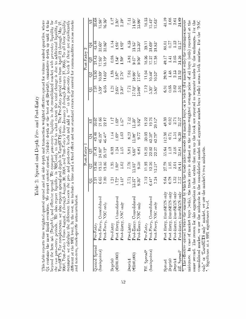
������������� �����������������������������������6�������7����������������6����,7��� �����������������-�����

����������������6����-7�����'��������������� �����!������������������������������ ���������!���������������

���������!������������������������������"#$!������0��������������������������������������������������������

%��#%�#� ��� ��������������������������������%��#%�#��������(�!%������������ &��)*������+��)��

),,-�(���!%������ &������)������&�����*,�),,-����(���!%���)�� .�����*������.�����*��),,/� �����������������

�����������������������'����������������!������!�����������������;<=��������!������������������������0������

��'���������335������>��������������������� �����0����'��������������������������������� ��������������������

������!���������!����0���������������

(���!%����

(���!%���)

��

�)

�*

�-

&��

��

�)

�*

�-

&��

������#���

(�!%���

2�3�

�*�4,

)��-*

-*�-4

),�12

2�3�

�*�4,

)��-*

-*�-4

),�14

6����������7

(���!%����$�����������

1�1/

�*�//

)-�4,�

-1�)4�

)��11

/�/3�

�,�43�

�2�3*�

*)�1,�

�/�34�

(���!%����"#$����

2�4,

�*�41

)/��*�

-1�-��

))��2

1�,/

���,*�

�4��3�

*)�41�

�1�)1�

����,

(�!%���

��)�

��*/

,�3*

���-

���2

��)�

��**

,�3*

���-

���2

6��,,�,,,7

(���!%����$�����������

��2)�

��4,�

��)-

��13�

��1*�

)�1/�

)�42�

��/-�

��3*�

)�*,�

(���!%����"#$����

��--�

��1)

���/

��1*

��-2�

)�*,�

)�24�

��/3�

��3)�

)��3�

����-

(�!%���

2�2�

2�21

/�4-

4�)*

2�-)

2�2�

2�1-

/�4-

4�)*

2�-�

6��,,�,,,7

(���!%����$�����������

�*�*2�

���3*�

4�11�

���,4�

���*3�

�2�/)�

�4�34�

3�-2�

���4/�

�-�4,�

(���!%����"#$����

3�*1�

3�/,

1�4-

3�22

4�3)�

�/�,1�

�2�,2�

3�/1�

�*�*,�

�*�31�

%'�#����

(�!%���

2��)

���3*

�4�)3

*3�,*

�4�))

2��)

���3-

�4�)1

*3���

�4�)*

6����������7

(���!%����$�����������

1�-��

�)�)1

))�,)

-)�/,�

�3�21

/�*,�

�,�--�

�2�)2

*��13�

�/�-)�

(���!%����"#$����

2�)-

�)�/��

))�)2

-)�2,�

),��/�

/�4,�

�,�/)�

�2�*4

*��4*�

�/�1*�

#���

(���!%����%��#%�#����

3�1-

)2�24

//�1-

��)�*1

-4�*3

1�3�

)3�4,

-3��2

44�,�

-���3

����,

(���!%����%��#%�#����

,�24

��,/

���*

,�2�

,�3)

,�1/

��-4

��-�

,�22

��,4

����-

(���!%����%��#%�#����

-�*)

)�1-

)��1

��/-

)�2-

)�1)

)��*

)�,/

���)

)�,�

%'�#����

(���!%����%��#%�#����

2�)2

�4�--

*)�4-

3��*3

*)�/2

/�3�

)��/)

*-��1

-���2

)-�43

�:����'��������������������� ����������������������������6�� ��������7��������6�� ���������7�������� �������

��������>������� ��������6�����7���������������0������������ �!��������������������������6�����7����������

�� ������������������������������������������������������������������������������������������� ����

������������ ������������� ������������������������ ��������������� ��������6�����7��������� ������ ����;"#$

����=�;%��#%�#����= ������������� ����?���� ��������

�

:#����0�������335�����0�����������

��

�������� �� � �������� ��������!�"����#"���� � ��#���� ��

��������������� �!��������������������������� �����!������!����������������������������� �����������������������

���� �������!���������������������������������������"#$!������������������������������������������ ������:������

���������������������6����,7������ �����������������-���������������������6����-7��������� ��������0������

���� ����������������������������6��������������7��������������������������������� ����������!����0� ���6��7�

������'���6�7������������������6���7���������� 6���7:

���@�

�����A�

�Æ ������������

�

A�

������A� ��

� ��@�

�� ���A�

� ���A��

��������� ��� �-������������������

����� ���������� ������0����'������� �������� ��'�����������������������������

������������� ���������������������� �����������(�!%������������ &��)*������+��)��),,-�(���!%������

&������)������&�����*,�),,-����(���!%���)�� .�����*������.�����*��),,/��!�����������������������������

�������������������������������!�����������������

(���!%����

(���!%���)

#���

����,

����-

#���

����,

����-

$������!

�����

"#$

$������!

�����

"#$

$������!

�����

"#$

$������!

�����

"#$

$������!

�����

"#$

$������!

�����

"#$

$�������6�7

!���1

!,��*

,�/1

,�*,

1�,,

)���

!��,/

!,�1)

��))

,�3,

4��2

1�)/

B���$��������!�-�25

!��15

-1�*5

)-�45

22�45

)2�-5

!�*�*5

!2�45

�,,�45

2-�-5

�,1�,5

4���5

�!�����

!-�22

!,�2)

-�2�

/�)*

�)�/4

/�/�

!)�4-

!��4�

/�*,

/�-*

�,�)*

2�14

$������)6Æ)7

!,�)4

!,�,/

,�1/

,�-*

/��)

)�-3

!��44

!��2-

��*)

��)�

3�2/

2�44

B���$������)�

!)�,5

!,�-5

-4��5

*��35

11�,5

*)��5

!�*�15

!�)�15

32�45

43�15

�)/�15

�,��/5

�!�����

!��,-

!,�),

)�2,

��3)

-�/1

)�),

!*�32

!*�14

)�-1

)�)2

)�31

)�*1

$������*6Æ*7

*�-3

*�23

,�**

,�)-

)�3)

��,2

!��2-

!��-)

,�**

,�*3

��/3

)���

B���$������*�

�1�*5

�2�25

*/�/5

)/�45

/,�,5

�4�*5

!4��5

!1�15

*/�/5

-��35

)2�)5

*1��5

�!�����

���4

��)3

��3�

��*4

*�,/

��*1

!,�14

!,�//

��,-

��,2

��*-

��,�

$������-6Æ-7

*���

*�)�

,�/2

,�/,

)�3,

��/)

!3�,1

!4�2*

,�/�

,�/,

��/-

*�-*

B���$������-�

2�)5

2�-5

/,�,5

-*�35

*/�)5

�4�/5

!),�45

!),��5

--�25

-*�35

�4�25

-��25

�!�����

��14

��22

)�3-

)�-2

-��,

)�),

!/�/1

!/�*�

��/4

��/*

��--

��13

�����9��� �

!,�),

!,�),

,�,1

,�,1

,�--

,�-/

!,�)4

!,�)4

,���

,���

,�43

,�4*

�!�����

!)�/�

!)�/�

)�33

*�,,

*��/

*�)4

!)�1,

!)�1/

*�,,

)�43

*�12

*�)1

�����9���������

)��4

)�)1

!,�-)

!,�-)

!)�-)

!)�*1

)�**

)�*1

!,�-1

!,�-4

!*�*,

!*�,*

�!�����

-�3*

/�,1

!*�/4

!*�-2

!*�-1

!*�*/

1�2,

2�,�

!)�31

!*��,

!*�1/

!*�*�

&�������(���

!,�,2

!,��,

,��,

,�,4

,�-3

,�*4

!,��4

!,�),

,�,)

,�,�

,�),

,�,/

�!�����

!,�1*

!,�43

)�2,

)�*�

)�-/

��34

!��)*

!��*1

,�-/

,�),

,�32

,�)�

B�

,�/*

,�/*

,�24

,�/)

,�-1

,�)4

,�/�

,�/�

,��4

,��-

,�)*

,��-

8C��

3),

3),

3),

3),

3),

3),

3),

3),

3),

3),

3),

3),

�:B����������!�����������

��

����� $� ��� ���� �! ��� ����� �� �! ��� %����� &��'

���� ����� ���� ���� ���� �� ��� ����?� ��� � ����� �������� �� ���: ��� ������ �� ����������� ��� ���� ���� � �� ��� ������ ����� � 6#CB#7� �� �������� ���� ������� �� ��������� �� �������������� ���� ������� �� ������� ����� ���� �� ��� %��#%�# ����� ���� ���� ���� ���� %��#%�#��� ������� ���� ���� ��� ����� ����� ���� �� ��� ������� ����� ����� � ����� ������������ �� ���������� ������ ���� ���������� �� %��#%�#� ��� �� � 0�� ��� �� ��� ������ �� � �� ����� ������� ��������� �� ���� ���� ��� ��� �� �� ��� 6���� ��� ;����!�������=7 ������ ���� �� � �� ��������� #CB#�� �� ������ ���� �� ���� �������� ��� #CB# ������� �� ���!#CB# ����� ���� ��������� �� �� � ���� ���������� �� ���� ��� ����� ;����= �� �������� %��#%�# ��� ���� ���� �� ������ ������ �� �������� ����� ���� ����������� �� ���� ��� � (BCD>� ���� ���� � ����� �� ����������������� ��� �� ���� � �� ����� �� ����� ��������� D���� ����� 6),,*7� �� ����� �� �'��� ����� ����������� E����� �� ���� ���:

��� @ (�F���� �� %��#%�#�#������ D���� %��#%�# �����G @ %F�� A ����� A ��� � ,G ��� � >>"6, �7

���� �� �� � �����!����0� �� � ��� ��� �������� %��#%�# ������ ����� ��� ����� 8����� �� ���, ������� ��� ���������� ����� �� ��� ������� ���� ���� ��� �� �� �, ������� �� ��� ��� ���� ������ ����� � �� �0��� ���� ��� �� �� �� ���� ����� �� ��� ������ �� %��#%�# ����� ������������� ������ ���� ���������� �� %��#%�#� D���� �� ��� ���� �� ��� ��������� ������ �� ��� (BCD>���������� �� ��� ��� ��������� �� ������ �� ����� ������: ��� �� %��#%�# ������ ���� ��� ���,�3,!�������� �� ��� ������������� 6����!���������7 ����������� �� ��� ����� ��� �� �� �� ������ �������������:

��� @ ���6��� @ ��7 @ H6I�� A I����7 �� @ F, ���6��7 ���6��7 ���6� 7G�

���� ���� �������� �������� ���� ���� ��� ���6�7 ��������� ��� ,�3,!�������� �� ��� ������������� 6����!���������7 ������������ (���� & ���� ���� �� ��� ���� (���� D ���� ��� (BCD>� �������� ���� ������!������� ��� ��������� ���� ����� ������� ��� ��� ���� ������ �� ��������� �� � ���!���� ������ �� ������������ �������� ��� J�� ��������� ������� ������ 6��7� ��� ��� ����� �� ����� ���� ��� ���������� �������� ����� �� �����0������ (���!%��� � ��� �� &������ ) ������ &����� *,� ),,- ��� (���!%���) �� .����� * ������ .����� *�� ),,/�

K��������� �� ���� ���K

�$

K��������� �� ������ ���K

����� �� ������ ��� ���� ��� � ����������� �� ��� �� �� ��(���!%��� � (���!%��� )

��(������%��#%�#�����

���(������%��#%�#����� ��&�����+����$���������

���� 8C��

��(������%��#%�#�����

���(������%��#%�#����� ��&�����+����$���������

���� 8C��

�� ,�/- ,�*2 ,�,� ))�)*3 ,�/- ,�*2 ,�,� �)�144�) ,�)) ,��/ ,�,) 122 ,��� ,�,/ ,�,) -2/�* ,��, ,�,/ ,�,/ -)* ,�,- ,�,) ,�,� )34�- ,�)* ,�), ,�,4 2) ,�,� ,�,� ,�,) 2)&�� ,�)2 ,��3 ,�,/ )*�-�� ,��4 ,��� ,�,) �*�/**

B�& ,�-* ,�)1 ,�,� /�)-4 ,�1� ,�-* ,�,� /�/4*>"L& ,�/, ,�** ,�,� *�1-� ,�/* ,�*1 ,�,� ��32)(E>& ,�/4 ,�-- ,�,� -�/)- ,�/* ,�*2 ,�,� ��21*&&D& ,�/2 ,�*2 ,�,� *��*1 ,�-1 ,�)3 ,�,� ��/)/&L" ,�12 ,�/) ,�,� *��2- ,�1) ,�-/ ,�,� 43� CB& ,�-4 ,�*� ,�,� )�/�1 ,�-2 ,�*, ,�,� 3/-&#+M ,��/ ,��� ,�,) �13 ,�)� ,��) ,�,* /1&E ,�*� ,�), ,�,) 3* ,�,3 ,�,* ,�,) �,2N(" ,�/1 ,�-� ,�,) 1� ,�,3 ,�,- ,�,) �,2&NO& ,��1 ,�,4 ,�,) �3, ,��2 ,�,4 ,�,* /-E%>& ,�,/ ,�,) ,�,� ��3 ,�,1 ,�,) ,�,) �,/B%" ,�,3 ,�,/ ,�,* -/ ,�,- ,�,� ,�,) -19"P& ,�,2 ,�,* ,�,� �2- ,�,1 ,�,) ,�,� ��2�#+ ,�,) ,�,, ,�,� �,/ ,�,, ,�,, ,�,, -3�NM ,��, ,�,/ ,�,* -� ,�,) ,�,� ,�,) -1�(L ,�,/ ,�,) ,�,) 33 ,��- ,�,/ ,�,) 11L�" ,�)/ ,��* ,��, - ,�,, ,�,, ,�,, ),>E$ ,�,* ,�,� ,�,) *4 ,�,, ,�,, ,�,, �-9B#& ,�,, ,�,, ,�,, ��EL+ ,�,, ,�,, ,�,� ) ,�,, ,�,, ,�,, )/DPEB ,�)* ,��2 ,�,* )1 ,�,, ,�,, ,�,, *+CC ,�12 ,�1� ,��/ 1 ,�,/ ,�,* ,�,/ �3�: ��� �������!����0� ��� ������ ���� ��� �� � �� ����� �� ������� �������� ������� ��� ��������� �� ��� ������� ��� �� ��� �����������

����� �� ��� �� ������� ������� �

$��� �!����� (!#��� � (!#���<������� ���� %��#%�# 6��,,�,,,7 ,�)�� )1�)2 ,�,4- ,�34- ,�,4)C�� #���� 6��,,�,,,7 !,�)12 !)*�4, !,��,2 ,�/�4 !,�,//8����� �� (�� �, +������ 6��,,, �����7 !,�*/1 !)�,4 !,��-) ,�,2, !,�,�,9���������� 6����������7 !,�,,* !2�41 !,�,,� )1�-)- !,�,*,�: &�� ����������� �� ��� �� � ������ �� ��������� ���� ��� ���� �� ��������� ������ ������ � ��� ���� �� ������ �������������: 9��������� �� ��0��� �� ��� ��� � ���� ��� ��� � ������� �� ��� ������ ��� ������ ������ �� ��� ������ ��������

��

��������������(%������ ���)��� ��������*���� ��� ����� �� � ����������� ������+

�����������������!������������������������������ ��������%��#%�#����������������������������� �����������#CB#

������:���������(����&���������������0�� �����:����������� �!��������"#$������%��#%�#����Q(����D��

��������� �����:���������%��#%�#��������������������������������� ����6%��#%�#�����������������������������

���7���������������������������������������� �����>��������������������������������������������:��������������� �

�������������������������!����������������������

(���!%����6"@)�7�

(���!%���)6"@))7

��

(������

%��#%�#

�����

���

(������

%��#%�#

�����

��

&�����

+����

$���������

���� �

6��,,�,,,7

����������

����������

657

B�

��

(������

%��#%�#

�����

���

(������

%��#%�#

�����

��

&�����

+����

$���������

���� �

6��,,�,,,7

����������

����������

657

B�

��������������� ��������� �!� ����"������� ������#������

6�7

,�/)3�

,�1,

��,�4�

,�44

6/�**7

6�)�,�7

6)7

,�/41�

,�-2

��-/)�

,�43

6-�,37

6�*�,17

6*7

,�*3*�

,�,,��

!,�,,-

,�22

��,�)�

,�,,,

,�,,*

,�43

6-�)*7

6)��27

6!��2-7

61�2/7

6,�-37

6��)37

6-7

,�-�2�

,�,,��

!,�,,-

,�2)

��-)-�

,�,,,

,�,,)

,�3,

6*�-/7

6)�147

6!��/27

62�)47

6,�-37

6,�327

��������������� ��������� �!� ���������#���� ���������� �����

6�7

,��/,

,��-

,�)/-�

,�1*

6��227

6/�417

6)7

,��//

,��,

,�*/)�

,�1�

6��-)7

6/�//7

6*7

,�,3*

,�,,,

!,�,,-

,�*-

,�),*�

,�,,,

!,�,,)

,�14

6��,)7

6,�/37

6!��237

6)�2�7

6,�)37

6!��/�7

6-7

,�,44

,�,,,

!,�,,-

,�*)

,�)13�

,�,,,

!,�,,)

,�12

6,�4�7

6,�4�7

6!��217

6)�/27

6,�-,7

6!��1/7

�: �9B#&��������������������������������������������������%��#%�#���������������������

��������������

�

:#����0�������3/5�����0�����������

�,

����� ,� ��� ���� �! ��� � ��-��. �� %��� ������ &�'

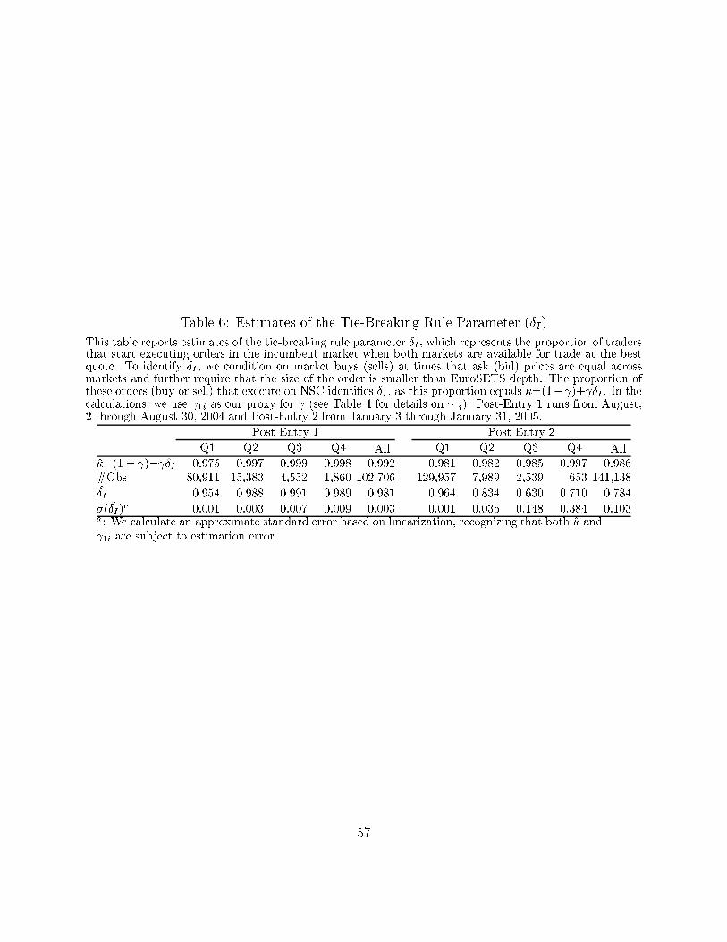
���� ����� ���� ���� ���� �� ��� ���!������� ��� �� ��� Æ � ����� ������� ��� ������ �� ��������� ���� ��������� ���� �� ��� ���� ���� ���� ���� ���� ����� �� ��������� �� ���� �� ��� ���������� �� �������� Æ � �� ��������� �� ���� ���� 6�����7 �� �� �� ���� ��� 6���7 ���� �� ����� ����� ����� ��� ����� ����� ���� ��� ���� �� ��� ��� �� � ���� ���� %��#%�# ����� ��� ������ ������� ���� 6��� � ����7 ���� ������� �� "#$ ������0�� Æ � �� ���� ������ ������ �@6���7A�Æ � >� ���������������� �� ��� �� �� �� ��� �� � 6��� ����� - �� ������� �� ��7� (���!%��� � ��� �� &������) ������ &����� *,� ),,- ��� (���!%��� ) �� .����� * ������ .����� *�� ),,/�

(���!%��� � (���!%��� )

�� �) �* �- &�� �� �) �* �- &��I�@6�� �7A�Æ ,�32/ ,�332 ,�333 ,�334 ,�33) ,�34� ,�34) ,�34/ ,�332 ,�3418C�� 4,�3�� �/�*4* -�//) ��41, �,)�2,1 �)3�3/2 2�343 )�/*3 1/* �-���*4IÆ ,�3/- ,�344 ,�33� ,�343 ,�34� ,�31- ,�4*- ,�1*, ,�2�, ,�24-

�6 IÆ 7� ,�,,� ,�,,* ,�,,2 ,�,,3 ,�,,* ,�,,� ,�,*/ ,��-4 ,�*4- ,��,*

�: �� ��������� �� ���� ��� ������� �� ����� �� ������������� ���������� ���� ���� I� ����� �� ���J��� �� ���� ����� ���

�/

����� /� 0������ ���� 1������� �����

���� ����� ���� ���� ���� �� ��� ������ ���� �� "#$!���� ����� ����� �� ���������� ����!���������� ����� ��� ���� ���� �������� �� "#$ ��� �!�������� 6�� ��7 ��� ��� �� %��#%�# �� ��� ������������� (���� & ���� ��� ����� ���� �� �� ������� ��������� ���� (���� D ���� ��� ����� ���� �� ���!�������� ��� ���� �� �� ��������� ���� (���� $ ���� ��� ��'������ (���!%��� � ��� �� &������) ������ &����� *,� ),,- ��� (���!%��� ) �� .����� * ������ .����� *�� ),,/�

(���!%��� � (���!%��� )

�� �) �* �- &�� �� �) �* �- &������� �� ��� ������ ��� ����$����$ %���

8 #��!C�� �� C��� �1�*2- ���2) 213 �4/ �4�/,, �,�13� 1/2 /�- )�) �)�,2- ������ �� ����� ,�,2 ,�,� ,�,� ,�,� ,�,- ,�,- ,�,� ,�,� ,�,� ,�,)+������ M���� 6���,,,7 *�* *3 )- 4 *4/ �2) �2 �� 3 ),4+������ "�� M���� 6���,,,7 )2� *2 )* 4 **4 �-* �1 �, 3 �22

����� �� ��� ������ ��� "� �� %���

8 #��!C�� �� C��� �/�3*4 ���-, 2/� �23 �4�,,4 �,�)1) 1*) -22 ),) ���/2* ������ �� ����� ,�,2 ,�,� ,�,� ,�,� ,�,- ,�,- ,�,, ,�,� ,�,, ,�,)+������ M���� 6���,,,7 *�* *3 )- 4 *4/ �2� �2 �� 3 ),4+������ "�� M���� 6���,,,7 )2� *2 )* 4 **3 �-* �1 �, 3 �22

����� �� ��&����� �� '��� ����� � ��� ����� � �� ��� ��

��'� +������ M��� 657 !,�,* !,�,* !,�,) !,�,/ !,�,* !,�,1 !,�,1 !,��1 !,�,1 !,�,1��'� +������ "�� M��� 657 ,�,- ,�,* ,�,) ,�,) ,�,- ,�,2 ,�,- ,��3 ,��- ,�,4�: � ��� �&� ����� �� ��� * ���� �� (���!%��� � ��� � ��� �� (���!%��� )� �� ��� ������������� ������ �� ���� ��� ��� � ���� �� ��� ���� ), ������ �����

�2

�

�

���������������������

��&�� � � � ��'

���

0�.�� � �� ������

���� �� 3 &�� �'��

�

�� 3 ����

�

0�.�������) �� 4�������

�.���� �����

5 ��� �� ��� � � �� 4������� 0�.�� �� ����� 6�7 5������� ������ 0��� ���������� �� ���� ������ �� 6� ��7 ��� ������ ���� �� ����������� ���� �� ���� � ��� ����� ���� �� ��������� � � �� ��� ���!���� ���� �� ��� ������ ����� ��� � �� ��� ������ �� #CB#���������

�8

����� �� ������ �

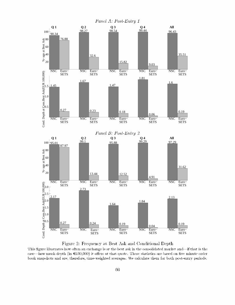
20

40

60

80

100

Q 1

90.34

76.88

NSC Euro−SETS

Q 298.27

32.6

NSC Euro−SETS

Q 398.54

15.82

NSC Euro−SETS

Q 499.44

9.03

NSC Euro−SETS

All96.43

35.51

NSC Euro−SETS

%−

age

at B

est A

sk

0.5

1.0

1.5 1.45

0.27

NSC Euro−SETS

1.67

0.23

NSC Euro−SETS

1.47

0.18

NSC Euro−SETS

1.81

0.06NSC Euro−

SETS

1.6

0.19

NSC Euro−SETS

Con

d. D

epth

at C

ons.

Bes

t Ask

(EU

R 1

00,0

00)

����� �� ������ �

20

40

60

80

100

Q 1

95.0187.97

NSC Euro−SETS

Q 299.1

13.44

NSC Euro−SETS

Q 395.88

12.52

NSC Euro−SETS

Q 499.29

4.91

NSC Euro−SETS

All97.29

31.62

NSC Euro−SETS

%−

age

at B

est A

sk

0.5

1.0

1.5

2.0

2.5

3.0

2.17

0.27

NSC Euro−SETS

2.73

0.24

NSC Euro−SETS

1.64

0.19

NSC Euro−SETS

1.84

0.04NSC Euro−

SETS

2.13

0.19

NSC Euro−SETS

Con

d. D

epth

at C

ons.

Bes

t Ask

(EU

R 1

00,0

00)

5 ��� �� 5������� �� -��� 9�. ��� ���� � ���� ��������� 0��� ���������� ��� ����� �� �������� �� �� ��� ���� ��� �� ��� ������������ ���� ���K�� ���� �� �������K��� ��� ���� 6�� ��,,�,,,7 �� �'�� �� ���� ������ ����� ���������� �� ����� �� 0��! ����� ������� �������� ��� ��� �������� �� �!�������� �������� �� ��������� ��� �� ���� ���!���� ������

,:

����� �� ������ �

� ���������

� ��������� ����� ���

� ��������� �������

� ��������� �������������

2.5

5.0

7.5

10.0

Q1

0.01 0.1 0.5 1 1.5 2

Bas

isPo

ints

Order Size (EUR 100,000)

510

1520

25

Q2

0.01 0.1 0.5 1 1.5 2

Bas

isPo

ints

Order Size (EUR 100,000)

∞ ∞∞

1020

3040

Q3

0.01 0.1 0.5 1 1.5 2

Bas

isPo

ints

Order Size (EUR 100,000)

∞ ∞∞ ∞∞

2550

75

Q4

0.01 0.1 0.5 1 1.5 2B

asis

Poin

ts

Order Size (EUR 100,000)

∞ ∞∞∞ ∞ ∞∞ ∞

����� �� ������ �

2.5

5.0

7.5

10.0

Q1

0.01 0.1 0.5 1 1.5 2

Bas

isPo

ints

Order Size (EUR 100,000)

510

15

Q2

0.01 0.1 0.5 1 1.5 2

Bas

isPo

ints

Order Size (EUR 100,000)

∞

1020

30 Q3

0.01 0.1 0.5 1 1.5 2

Bas

isPo

ints

Order Size (EUR 100,000)

∞ ∞ ∞

2550

75

Q4

0.01 0.1 0.5 1 1.5 2

Bas

isPo

ints

Order Size (EUR 100,000)

∞ ∞∞∞ ∞

5 ��� �� � �� � �� ����� ���� ��� ��� ������������� 0��� ���������� ��� �� �!�������� ���� �� �� ������ ��������� �! ��� ���!����� �� ��������� ���������� ��� � ��� 6�� ��� �������7 �� ����������� ��� ���� �� ���� ���,,, ������ �),,�,,, ������� 0��! ����� ��� ���� ������� �������� &� �� ���� ���� ��� 0�� ���� ���� ��� ���� ������ ����������� 6�������7 ������ ����� ������ �� ��� ��� ���� ��� 0�� �� ����� ����� >�� ������� ���� �������� ����� 6��,57� �� ��� ���� �� ��0���� 6�7 �� �������� ���� �� �� ������ �� ���� ���� ���� ����� � ���� �� ����� ��� ��� �������� �!���� ����� ���!���� ���� �� ��� ������������ ����� ���!���� ����"#$ ����� ��� ���!���� ���� %��#%�# ����� ,�