competitive interactions moderate the effects of elevated
TRANSCRIPT
1
The following supplement accompanies the article
Competitive interactions moderate the effects of elevated temperature and atmospheric CO2 on the health and
functioning of oysters
Dannielle Senga Green*, Hazel Christie, Nicola Pratt, Bas Boots, Jasmin A. Godbold, Martin Solan, Chris Hauton
*Corresponding author: [email protected]
Marine Ecology Progress Series 582: 93–103 (2017)
Supplement 1. Summary of statistical models
We present the data for each response variable including mean ± standard error for each treatment level. For each response variable, we started with an initial linear regression model of the form: [Dependent variable] ~ Temp + CO2 + Oyster + Temp×CO2 + Temp×Oyster + CO2×Oyster + Temp×CO2×Oyster Abbreviations: Temp = Temperature (2 levels; 12°C or 16°C) CO2 = atmospheric [CO2] (2 levels; ambient [400ppm] versus elevated [1000ppm]) Oyster = species composition within each mesocosm (6 levels; two individuals of C. gigas; two individuals of O. edulis; one C. gigas with one O. edulis; one O. edulis with one C. gigas; a single C. gigas; a single O. edulis] Where it was necessary to account for violation of homogeneity of variance, we used a linear regression with GLS estimation. All independent factors were treated as nominal and we carried out a manual backwards selection procedure to refine each model. The minimal adequate model is shown for each response variable.
2
Supplement 2. Model S1 | FILTRATION (N = 140) Minimal adequate model: Filtration ~ Oyster, weights = varIdent(form = ~ 1|Oyster), method = "ML")
Figure S1. Variance plots of the baseline model (full factorial) and the minimal adequate linear regression model after weighting among variance covariates and backwards step-wise elimination of insignificant terms for response variable Filtration. Table S1a. Contribution of factors from the minimal adequate model to Filtration rates. d.f.1 AIC2 L- Ratio3 P-value
Full model 30 533.5
Oyster 5 538.7 34.47 <0.001 1 Degrees of freedom 2 Akaike information criterion 3 Likelihood ratio
3
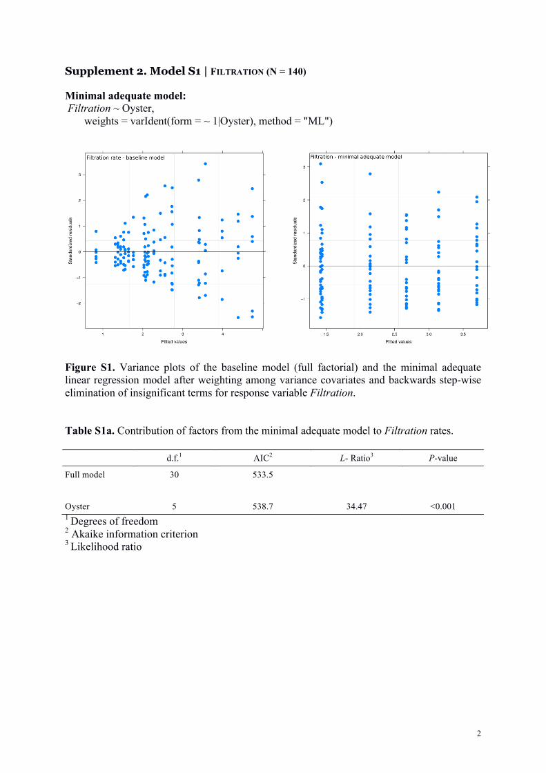
Table S1b. Pairwise comparisons of Filtration for all levels in “Oyster”. Data are coefficients ± standard error (in italics) and underneath the t-values with superscript P-values in parentheses comparing row to column levels. The relevant species composition comparisons are highlighted in bold. Intra C. gigas Intra O. edulis Inter C. gigas Inter O. edulis Single C. gigas Single O. edulis
Intra C. gigas1
-
Intra O. edulis2 2.227 ± 0.566 (4.03<0.001)
-
Inter C. gigas3 0.557 ± 0.695 (0.800.424)
-1.721 ± 0.467 (-3.68<0.001)
-
Inter O. edulis4 2.256 ± 0.562 (4.01<0.001)
-0.021 ± 0.228 (-0.090.927)
1.700 ± 0.463 (3.67<0.001)
-
Single C. gigas5 1.026 ± 0.668 (1.540.127)
-1.251 ± 0.426 (-2.940.004)
0.469 ± 0.586 (0.800.425)
-1.230 ± 0.421 (-2.920.004)
-
Single O. edulis6 1.554 ±0.605 (2.570.011)
-0.724 ± 0.319 (-2.270.025)
0.997 ± 0.514 (1.940.054)
-0.703 ± 0.312 (-2.250.026)
0.528 ± 0.476 (1.110.270)
-
1 Crassostrea gigas in intraspecific competition (i.e. with other C. gigas). 2 Ostrea edulis in intraspecific competition (i.e. with other O. edulis). 3 C. gigas in interspecific competition (i.e. with O. edulis). 4 O. edulis in interspecific competition (i.e. with C. gigas). 5 C. gigas with no competition. 6 O. edulis with no competition.
4
Supplement 3. Model S2 | RESPIRATION (N = 108) Minimal adequate model: Respiration ~ Oyster, weights = varIdent(form=~1|CO2×Oyster), method = "ML")
Figure S2. Variance plots of the baseline model (full factorial) and the minimal adequate linear regression model after weighting among variance covariates and backwards step-wise elimination of insignificant terms response variable Respiration. Table S2a. Contribution of factors from the minimal adequate model to Respiration. d.f. AIC L- Ratio P-value
Full model 36 -36.6
Oyster 5 -35.8 21.44 <0.001

5
Table S2b. Pairwise comparisons of Respiration for all levels in “Oyster”. Data are coefficients ± standard error (in italics) with underneath the t-values and superscript P-values in parentheses, comparing row to column levels. The relevant species composition comparisons are highlighted in bold. Intra C. gigas Intra O. edulis Inter C. gigas Inter O. edulis Single C. gigas Single O. edulis
Intra C. gigas
-
Intra O. edulis -0.055 ± 0.033 (-1.630.105)
-
Inter C. gigas -0.004 ± 0.038 (-0.090.927)
0.058 ± 0.044 (1.320.191)
-
Inter O. edulis -0.184 ± 0.048 (-3.87<0.001)
-0.129 ± 0.052 (-2.470.015)
-0.187 ± 0.056 (-3.370.001)
-
Single C. gigas -0.171 ± 0.047 (-3.64<0.001)
-0.117 ± 0.052 (-2.240.027)
-0.175 ± 0.055 (-3.170.002)
0.013 ± 0.062 (0.200.839)
-
Single O. edulis -0.065 ± 0.037 (-1.780.078)
-0.011 ± 0.043 (-0.250.802)
-0.069 ± 0.047 (-1.470.144)
0.119 ± 0.555 (2.170.032)
0.106 ± 0.054 (1.950.054)
-

6
SUPPLEMENT 4. MODEL S3 | HAEMOCYTES (N = 140) Minimal adequate model: Haemocytes ~ Temp + CO2 + Oyster +
Temp×CO2 + CO2×Oyster, weights = varIdent(form = ~ 1|CO2×Oyster), method = "ML")
Figure S3. Variance plots of the baseline model (full factorial) and the minimal adequate linear regression model after weighting among variance covariates and backwards step-wise elimination of insignificant terms. Table S3a. Contribution of factors from the minimal adequate model to Haemocytes. d.f. AIC L- Ratio P-value
Full model 36 1034.3
Temp 2 1095.9 9.14 0.010
CO2 5 1029.3 23.58 0.001
Oyster 10 1021.9 22.28 0.014
Temp×CO2 5 1023.9 14.22 0.014
CO2×Oyster 1 1026.7 9.04 0.003

7
Table S3b. Pairwise comparisons of Haemocytes for all levels in “Temp×CO2”. Data are coefficients ± standard error (in italics) with underneath the t-values with superscript P-values in parentheses, comparing row to column levels. Temp 12°C 16°C
Temp CO2 400 ppm 1000 ppm 400 ppm 1000 ppm
12°C 400 ppm -
1000 ppm -2.003 ± 1.925 (-1.040.300)
-
16°C 400 ppm -5.188 ± 2.211 (-2.350.020)
-3.184 ± 1.907 (-1.670.097)
-
1000 ppm 1.039 ± 1.875 (0.550.580)
3.043 ± 1.505 (2.020.045)
6.277 ± 1.857 (3.350.001)
-
8
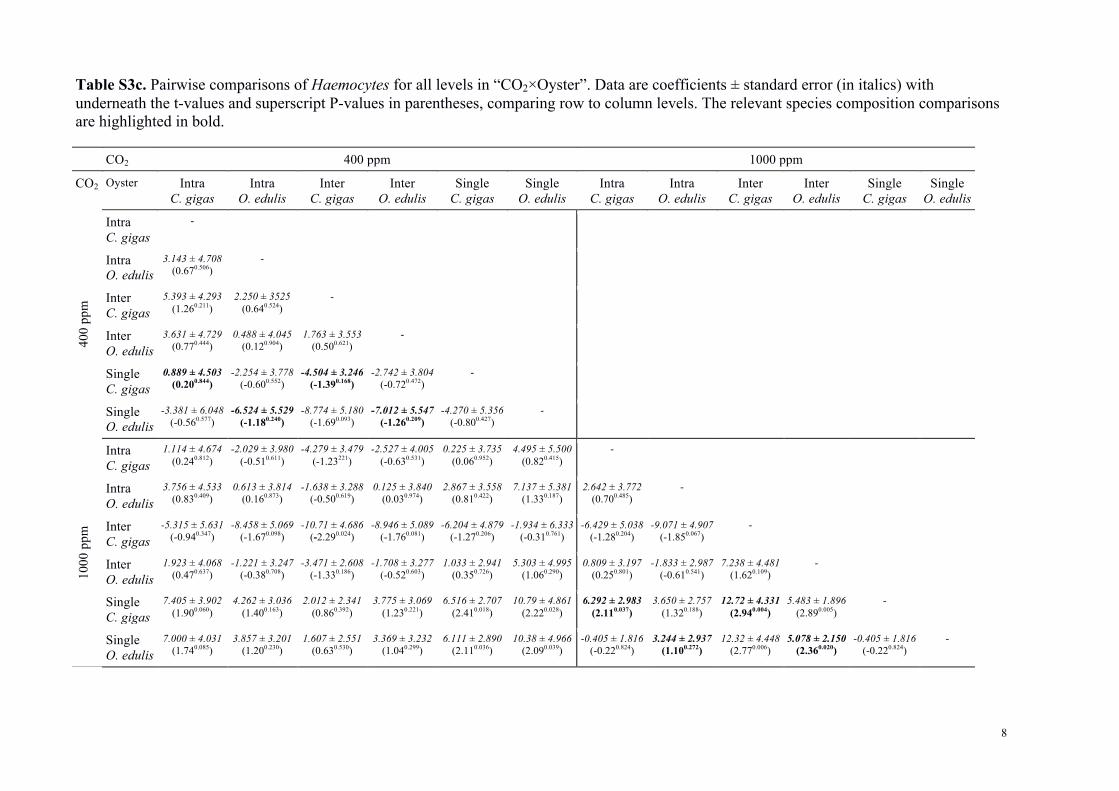
Table S3c. Pairwise comparisons of Haemocytes for all levels in “CO2×Oyster”. Data are coefficients ± standard error (in italics) with underneath the t-values and superscript P-values in parentheses, comparing row to column levels. The relevant species composition comparisons are highlighted in bold. CO2 400 ppm 1000 ppm
CO2 Oyster Intra C. gigas
Intra O. edulis
Inter C. gigas
Inter O. edulis
Single C. gigas
Single O. edulis
Intra C. gigas
Intra O. edulis
Inter C. gigas
Inter O. edulis
Single C. gigas
Single O. edulis
400
ppm
Intra C. gigas
-
Intra O. edulis
3.143 ± 4.708 (0.670.506)
-
Inter C. gigas
5.393 ± 4.293 (1.260.211)
2.250 ± 3525 (0.640.524)
-
Inter O. edulis
3.631 ± 4.729 (0.770.444)
0.488 ± 4.045 (0.120.904)
1.763 ± 3.553 (0.500.621)
-
Single C. gigas
0.889 ± 4.503 (0.200.844)
-2.254 ± 3.778 (-0.600.552)
-4.504 ± 3.246 (-1.390.168)
-2.742 ± 3.804 (-0.720.472)
-
Single O. edulis
-3.381 ± 6.048 (-0.560.577)
-6.524 ± 5.529 (-1.180.240)
-8.774 ± 5.180 (-1.690.093)
-7.012 ± 5.547 (-1.260.209)
-4.270 ± 5.356 (-0.800.427)
-
1000
ppm
Intra C. gigas
1.114 ± 4.674 (0.240.812)
-2.029 ± 3.980 (-0.510.611)
-4.279 ± 3.479 (-1.23221)
-2.527 ± 4.005 (-0.630.531)
0.225 ± 3.735 (0.060.952)
4.495 ± 5.500 (0.820.415)
-
Intra O. edulis
3.756 ± 4.533 (0.830.409)
0.613 ± 3.814 (0.160.873)
-1.638 ± 3.288 (-0.500.619)
0.125 ± 3.840 (0.030.974)
2.867 ± 3.558 (0.810.422)
7.137 ± 5.381 (1.330.187)
2.642 ± 3.772 (0.700.485)
-
Inter C. gigas
-5.315 ± 5.631 (-0.940.347)
-8.458 ± 5.069 (-1.670.098)
-10.71 ± 4.686 (-2.290.024)
-8.946 ± 5.089 (-1.760.081)
-6.204 ± 4.879 (-1.270.206)
-1.934 ± 6.333 (-0.310.761)
-6.429 ± 5.038 (-1.280.204)
-9.071 ± 4.907 (-1.850.067)
-
Inter O. edulis
1.923 ± 4.068 (0.470.637)
-1.221 ± 3.247 (-0.380.708)
-3.471 ± 2.608 (-1.330.186)
-1.708 ± 3.277 (-0.520.603)
1.033 ± 2.941 (0.350.726)
5.303 ± 4.995 (1.060.290)
0.809 ± 3.197 (0.250.801)
-1.833 ± 2.987 (-0.610.541)
7.238 ± 4.481 (1.620.109)
-
Single C. gigas
7.405 ± 3.902 (1.900.060)
4.262 ± 3.036 (1.400.163)
2.012 ± 2.341 (0.860.392)
3.775 ± 3.069 (1.230.221)
6.516 ± 2.707 (2.410.018)
10.79 ± 4.861 (2.220.028)
6.292 ± 2.983 (2.110.037)
3.650 ± 2.757 (1.320.188)
12.72 ± 4.331 (2.940.004)
5.483 ± 1.896 (2.890.005)
-
Single O. edulis
7.000 ± 4.031 (1.740.085)
3.857 ± 3.201 (1.200.230)
1.607 ± 2.551 (0.630.530)
3.369 ± 3.232 (1.040.299)
6.111 ± 2.890 (2.110.036)
10.38 ± 4.966 (2.090.039)
-0.405 ± 1.816 (-0.220.824)
3.244 ± 2.937 (1.100.272)
12.32 ± 4.448 (2.770.006)
5.078 ± 2.150 (2.360.020)
-0.405 ± 1.816 (-0.220.824)
-
9
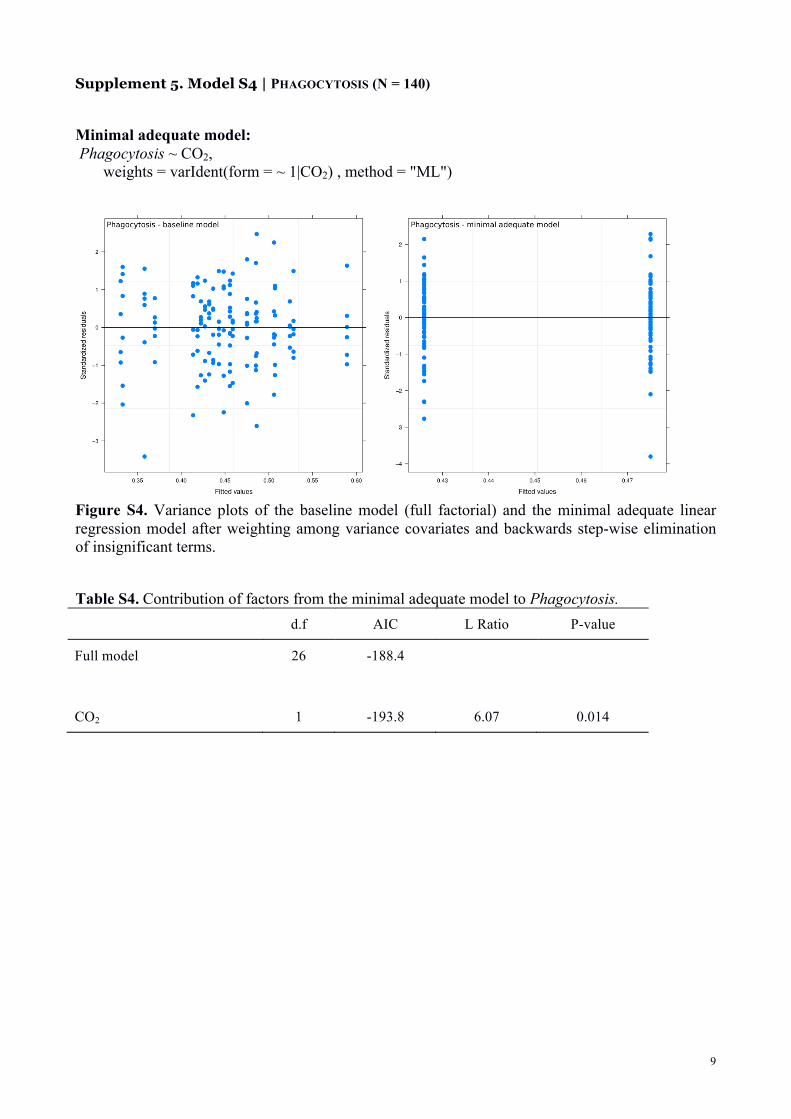
Supplement 5. Model S4 | PHAGOCYTOSIS (N = 140) Minimal adequate model: Phagocytosis ~ CO2, weights = varIdent(form = ~ 1|CO2) , method = "ML")
Figure S4. Variance plots of the baseline model (full factorial) and the minimal adequate linear regression model after weighting among variance covariates and backwards step-wise elimination of insignificant terms. Table S4. Contribution of factors from the minimal adequate model to Phagocytosis. d.f AIC L Ratio P-value
Full model 26 -188.4
CO2 1 -193.8 6.07 0.014
10
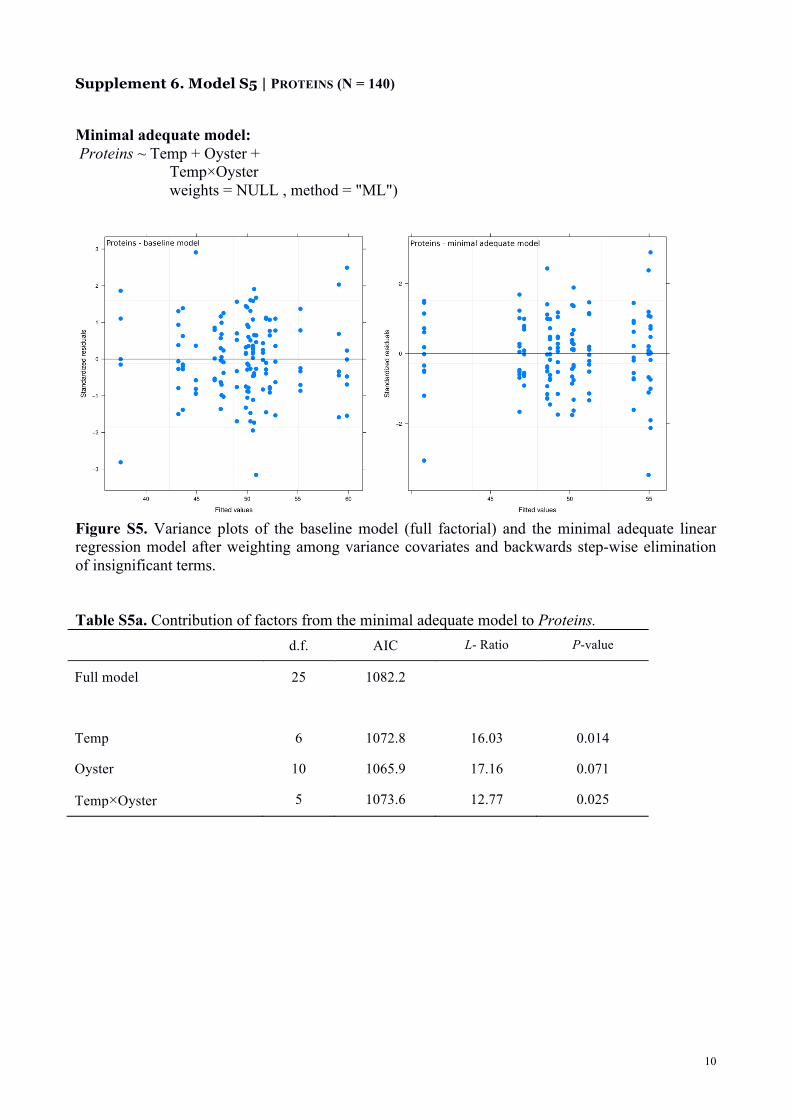
Supplement 6. Model S5 | PROTEINS (N = 140) Minimal adequate model: Proteins ~ Temp + Oyster +
Temp×Oyster weights = NULL , method = "ML")
Figure S5. Variance plots of the baseline model (full factorial) and the minimal adequate linear regression model after weighting among variance covariates and backwards step-wise elimination of insignificant terms. Table S5a. Contribution of factors from the minimal adequate model to Proteins. d.f. AIC L- Ratio P-value
Full model 25 1082.2
Temp 6 1072.8 16.03 0.014
Oyster 10 1065.9 17.16 0.071
Temp×Oyster 5 1073.6 12.77 0.025
11
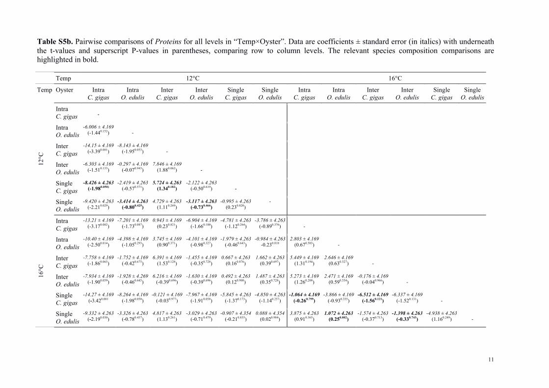
Table S5b. Pairwise comparisons of Proteins for all levels in “Temp×Oyster”. Data are coefficients ± standard error (in italics) with underneath the t-values and superscript P-values in parentheses, comparing row to column levels. The relevant species composition comparisons are highlighted in bold. Temp 12°C 16°C
Temp Oyster Intra C. gigas
Intra O. edulis
Inter C. gigas
Inter O. edulis
Single C. gigas
Single O. edulis
Intra C. gigas
Intra O. edulis
Inter C. gigas
Inter O. edulis
Single C. gigas
Single O. edulis
12°C
Intra C. gigas
-
Intra O. edulis
-6.006 ± 4.169 (-1.440.152)
-
Inter C. gigas
-14.15 ± 4.169 (-3.390.001)
-8.143 ± 4.169 (-1.950.053)
-
Inter O. edulis
-6.303 ± 4.169 (-1.510.133)
-0.297 ± 4.169 (-0.070.943)
7.846 ± 4.169 (1.880.062)
-
Single C. gigas
-8.426 ± 4.263 (-1.980.050)
-2.419 ± 4.263 (-0.570.571)
5.724 ± 4.263 (1.340.182)
-2.122 ± 4.263 (-0.500.619)
-
Single O. edulis
-9.420 ± 4.263 (-2.210.029)
-3.414 ± 4.263 (-0.800.425)
4.729 ± 4.263 (1.110.269)
-3.117 ± 4.263 (-0.730.466)
-0.995 ± 4.263 (0.230.820)
-
16°C
Intra C. gigas
-13.21 ± 4.169 (-3.170.002)
-7.201 ± 4.169 (-1.730.087)
0.943 ± 4.169 (0.230.821)
-6.904 ± 4.169 (-1.660.100)
-4.781 ± 4.263 (-1.120.264)
-3.786 ± 4.263 (-0.890.376)
-
Intra O. edulis
-10.40 ± 4.169 (-2.500.014)
-4.398 ± 4.169 (-1.050.293)
3.745 ± 4.169 (0.900.371)
-4.101 ± 4.169 (-0.980.327)
-1.979 ± 4.263 (-0.460.643)
-0.984 ± 4.263 -0.230.818
2.803 ± 4.169 (0.670.503)
-
Inter C. gigas
-7.758 ± 4.169 (-1.860.065)
-1.752 ± 4.169 (-0.420.675)
6.391 ± 4.169 (1.530.128)
-1.455 ± 4.169 (-0.350.728)
0.667 ± 4.263 (0.160.876)
1.662 ± 4.263 (0.390.697)
5.449 ± 4.169 (1.310.194)
2.646 ± 4.169 (0.630.527)
-
Inter O. edulis
-7.934 ± 4.169 (-1.900.059)
-1.928 ± 4.269 (-0.460.645)
6.216 ± 4.169 (-0.390.696)
-1.630 ± 4.169 (-0.390.696)
0.492 ± 4.263 (0.120.908)
1.487 ± 4.263 (0.350.728)
5.273 ± 4.169 (1.260.208)
2.471 ± 4.169 (0.590.554)
-0.176 ± 4.169 (-0.040.966)
-
Single C. gigas
-14.27 ± 4.169 (-3.420.001
-8.264 ± 4.169 (-1.980.050)
-0.121 ± 4.169 (-0.030.977)
-7.967 ± 4.169 (-1.910.058)
-5.845 ± 4.263 (-1.370.173)
-4.850 ± 4.263 (-1.140.257)
-1.064 ± 4.169 (-0.260.799)
-3.866 ± 4.169 (-0.930.355)
-6.512 ± 4.169 (-1.560.121)
-6.337 ± 4.169 (-1.520.131)
-
Single O. edulis
-9.332 ± 4.263 (-2.190.030)
-3.326 ± 4.263 (-0.780.437)
4.817 ± 4.263 (1.130.261)
-3.029 ± 4.263 (-0.710.479)
-0.907 ± 4.354 (-0.210.835)
0.088 ± 4.354 (0.020.984)
3.875 ± 4.263 (0.910.365)
1.072 ± 4.263 (0.250.802)
-1.574 ± 4.263 (-0.370.713)
-1.398 ± 4.263 (-0.330.743)
-4.938 ± 4.263 (1.160.249)
-
12
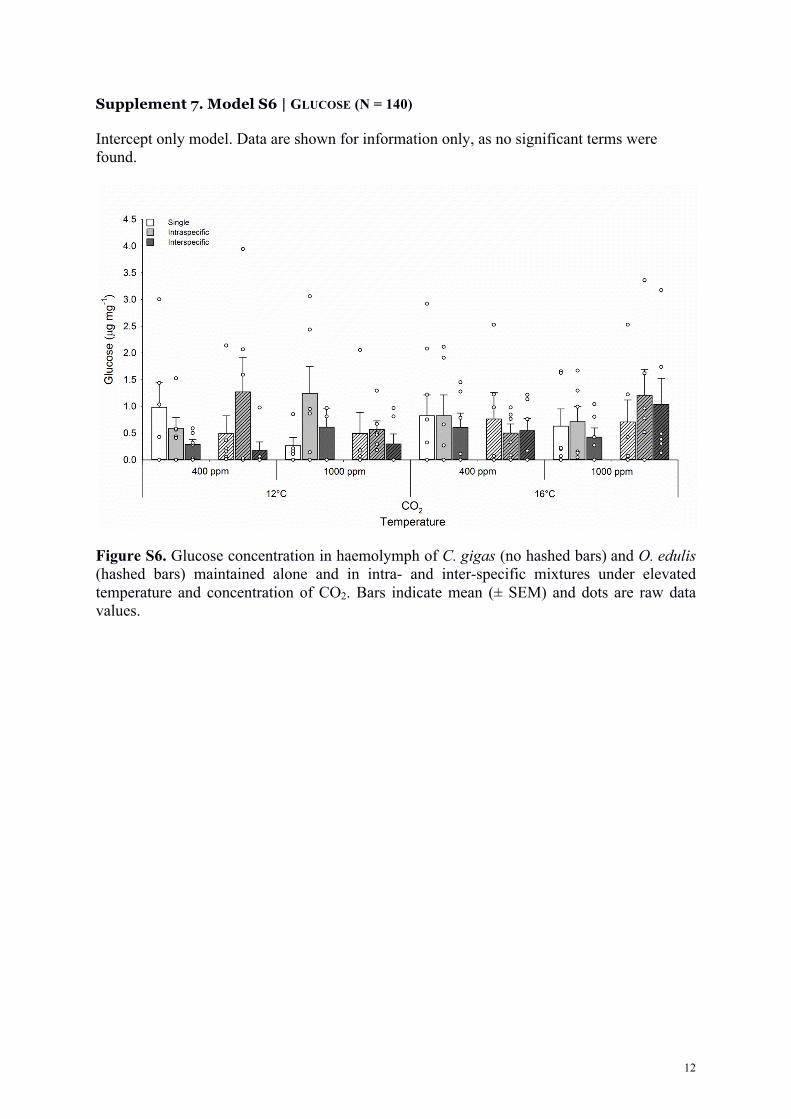
Supplement 7. Model S6 | GLUCOSE (N = 140) Intercept only model. Data are shown for information only, as no significant terms were found.
Figure S6. Glucose concentration in haemolymph of C. gigas (no hashed bars) and O. edulis (hashed bars) maintained alone and in intra- and inter-specific mixtures under elevated temperature and concentration of CO2. Bars indicate mean (± SEM) and dots are raw data values.