complete solution of the extended eoq repair and waste ... · the economic order quantity model...
TRANSCRIPT

Complete Solution of the Extended EOQ Repair and Waste Disposal Model with Switching Costs
Nadezhda Kozlovskaya
Nadezhda Pakhomova
Knut Richter
___________________________________________________________________
European University Viadrina Frankfurt (Oder)
Department of Business Administration and Economics
Discussion Paper No. 376
November 2015
ISSN 1860 0921
___________________________________________________________________

Complete Solution of the Extended EOQ Repair
and Waste Disposal Model with Switching Costs
Nadezhda Kozlovskaya1∗, Nadezhda Pakhomova2, Knut Richter3
1 Saint Petersburg State University,Chaikovskogo 62,191123,St.Petersburg, Russia
[email protected] Saint Petersburg State University,
Chaikovskogo 62,191123,St.Petersburg, [email protected]
3Saint Petersburg State University,Chaikovskogo 62,191123,St.Petersburg, Russia
European University ViadrinaFrankfurt (Oder), Germany
Abstract: The EOQ repair and waste disposal problem was studied firstby Richter, 1997. A first shop is providing a homogeneous product used bya second shop at a constant demand rate. The first shop is manufacturingnew products and it is also repairing products used by a second shop, whichare then regarded as being as good as new. The products are employed by asecond shop and collected there according to a repair rate. The other productsare immediately disposed of as waste. At the end of some period of time,the collected products are brought back to the first shop and will be storedas long as necessary and then repaired. If the repaired products are finished,the manufacturing process starts to cover the remaining demand for the timeinterval. The model was extended by Saadany and Jaber, 2008 to the problemof minimizing the total cost of production, remanufacturing and inventory whileincorporating additional switching costs. The switching cost is incurred whenthe process shifts from repair to production and from production to repair.However, in their paper the authors did not provide a complete solution to thiscomplex problem. We provide the solution in this paper.
Keywords: EOQmodel, Production/recovery, Reuse, Waste disposal, Switch-ing cost
∗The work is supported by Saint Petersburg State University grant 0.50.2097.2013.

1 Introduction
In recent years, reverse logistics has been receiving increasing attention fromacademia and industry.
There is increasing recognition that careful management can bring both en-vironmental protection and lower costs; environmental and economic consider-ations have led to manufacturers taking their products back at the end of theirlifetime. As a result, the reverse logistics process is now considered to be a basisfor generating real economic value and to provide support for environmentalconcerns.
Rogers and Tibben-Lembke, 1998 [25] defined reverse logistics as the processof planning, implementing and controlling the efficient and cost effective flow ofraw materials, in-process inventory, finished goods and related information fromthe point of consumption to the point of origin for the purpose of recapturingvalue or proper disposal.
The integration of forward and reverse supply chains resulted in the origi-nation of the concept of a closed-loop supply chain. The whole chain can bedesigned in such a way that it can service both forward and reverse processesefficiently.
Akcalı and Cetinkaya, 2011 [1] published the most recent review of quanti-tative modelling for inventory and production planning in a closed-loop supplychain.
Inventory models are divided according to modelling demand and returnprocesses into two main categories: deterministic and stochastic. The subject ofthis paper is deterministic inventory models with constant demand and return.The economic order quantity model (EOQ model), which was derived by FordW. Harris in 1913, became the basis for many reverse logistics models because ofits simplicity and intelligibility. Andriolo et al., 2014 [2] provided a most detailedreview in their work on the EOQ problem. Shrady, 1967 [29] was the first toapply the EOQ model to reverse logistics processes. He introduced an EOQmodel with instantaneous production and repair rates. A closed-form solutionwas developed. In his work an efficient policy P (m, 1) was established, whichmeans that within each remanufacturing cycle a number m of remanufacturingbatches of equal size are followed by exactly one manufacturing batch.
This work was extended by Nahmias and Rivera, 1979 [19] and Mabini et al.,1992 [18] extended Shrady’s model to the multi-item case. Koh et al., 2002 [11]analysed a model similar to that of Shrady, 1967 [29], but with some differences.They considered two types of policies,P (m, 1) and P (1, n), under a limited repaircapacity, where n is the number of manufacturing batches. They examined thecases of a smaller and a larger recovery rate compared to the demand rate.
Teunter, 2001 [31] generalized the results of Schrady by examining differentstructures of the remanufacturing cycle. He considered different types of policiesby placing the n manufacturing batches and m recovery batches in differentorders. He concluded that the policy P (m,n),m > 1, n > 1 will never beoptimal if the above-mentioned m and n are simultaneously larger than one,and that only the two policies P (1, n) and P (m, 1) are relevant.
2

Choi et al., 2007 [4] generalized the P (m,n) policy of Teunter by consideringthe ordered sequence of manufacturing and remanufacturing batches within thecycle as decision variables. Through sensitivity analysis they found that only0.2% out of the 8,100,000 tested instances of the model have an optimal solutionwith both m and n greater than one. Liu et al., 2009 [17] generated and solved60,000 instances and found that only 0.19% of them have an optimal solution inP (m,n) with both m and n greater than one. Konstantaras and Papachristos,2008 [14] extended Teunters approach and found the exact solutions for theoptimal numbers m and n.
In the literature two different types of problems are considered. Some au-thors have searched for an optimal policy P (m,n) that involves determiningthe optimal number of manufacturing and remanufacturing batches (we callthis problem ”ONB”) for given recovery or waste disposal rates β or α. Othershave tried to go further by determining the optimal recovery or waste disposal(we call this problem ”OWDR”).
Richter was the author of a series of papers where he considered an EOQmodel with respect to the waste disposal problem. Richter, 1996 [21] proposedan EOQ model that differed from that of Shrady, who assumed a continuousflow of used products to the manufacturer. Richter, 1996 [21] assumed a systemof two shops: the first shop provided a product used by a second shop; thefirst shop manufactures new products and repairs (in contemporary terms—remanufactures) products already used by the second shop and collected thereaccording to some rate; other products are disposed of according to a disposalrate. At the end of a certain time interval the collected items are brought backto the first shop. Richter, 1997 [23] examined the optimal inventory holdingpolicy if the waste disposal (return) rate is a decision variable. The result ofthis study was that the optimal policy has an extremal property: either reuseall items without disposal or dispose of all items and produce new products;that is, the policy of the type P (m,n) with m > 1 and n > 1 is never optimal.He also derived a closed-form for the optimal policy parameters. This analysisof the repair and waste disposal model was continued in the papers by Richterand Dobos, 1999 [24] and Dobos and Richter, 2000 [5].
Dobos and Richter, 2003 [6] and Dobos and Richter, 2004 [7] studied aproduction/recycling system with constant demand that is satisfied by non-instantaneous production and recycling. They concluded that it is optimaleither to produce or to recycle all items that are brought back. Dobos andRichter, 2006 [8] extended their previous work by considering the quality of thereturned items.
Saadany and Jaber 2010 [27] argued that such a pure policy of no wastedisposal is technologically infeasible and suggested the introduction of a de-mand function that depends on two decision variables: purchasing price andacceptance quality level.
Saadany et al., 2012 [28] regarded the assumption that an item can be re-covered indefinitely as unrealistic: material degrades in the process of recyclingand loses some of its mass and quality, thereby making the option of multiple re-covery somewhat infeasible. Saadany et al., 2012 [28] developed a model where
3

an item can be recovered only a finite number of times.Some authors extended the above-mentioned models to take account of var-
ious assumptions. One option is to allow for backorders, where some customersare compensated for having to wait for their delayed orders by either a reductionin price or some other form of discount, which is a cost incurred by the sup-plying firm. This results in a backorder cost. Konstantaras and Papachristos,2006 [13] extended the work of Richter, 1996 [21] by allowing for backordersin remanufacturing and production while keeping the other assumptions thesame. Saadany and Jaber, 2009 [10] extended the work of Richter, 1996 [21] byassuming that demand for manufactured items is different from that for remanu-factured (repaired) items. This assumption results in lost sales situations wherethere are stock-out periods for manufactured and remanufactured items; thatis, demand for newly manufactured items is lost during remanufacturing cyclesand vice versa. In the study of Konstantaras et al., 2010 [16], which extendedthe work of Koh et al., 2002 [11], a combined inspection and sorting process isintroduced with a fixed setup cost and unit variable costs. This study assumesthat remanufactured and newly purchased products are sold in a primary mar-ket whereas refurbished units are sold in a secondary market. Konstantaras andScouri, 2010 [15] considered two models: one with no shortages and the otherwith shortages. Both models are considered for the case of variable setup num-bers of equal sized batches for the production and remanufacturing processes.For these two models, sufficient conditions for the optimal type of policy, refer-ring to the parameters of the models, are proposed. Hasanov et al., 2012 [9]extended the work of Jaber and Saadany, 2009 [10] for the full-backorder andpartial-backorder cases, where recovered items (remanufactured or repaired) areperceived by customers to be of lower quality; that is, not as good as new items.
Pishchulov et al., 2014 [20] studied a closed-loop supply chain in which asingle purchaser orders a particular product from a single vendor and sells it onthe market. A certain fraction of used items are returned to the purchaser fromthe market. The latter is responsible for collecting and returning them to thevendor. In addition to manufacturing new items, the vendor is able to remanu-facture the returns into items that are as good as new and are subsequently usedto meet the demand from the market. The questions addressed by this studypertain to the optimal centralized control of this closed-loop supply chain, theindividually optimal policies of its members and the coordination within thissupply chain under a decentralized control.
However, for some of the above-mentioned models, so far no complete solu-tions have been presented. In the paper of Saadany and Jaber, 2008 [26] theextended EOQ production, repair and waste disposal model of Richter, 1996[21] was modified to show that ignoring the first time interval results in an un-necessary residual inventory and consequently an over estimation of the holdingcosts. They also introduced switching costs in order to take into account pro-duction losses, deterioration in quality or additional labour. When shifting fromproducing (performing) one product (job) to another in the same facility, thefacility may incur additional costs, referred to as switching costs, when alternat-ing between production and repair runs. The special case of even numbers m
4

and n was studied and conditions were provided to decide which of two policiesP (m,n) and P (m2 ,
n2 ) is preferable, but a general optimal policy for the problem
was not presented. In our study we will provide a general optimal solution forthe model.
Our paper is organized in the following way: in the second section, the as-sumptions and notations are presented; in the third section, the extended EOQproduction, repair and waste disposal model, with switching costs, is formu-lated and analysed; in the fourth section, the ONB problem is studied, an exactoptimal policy is derived and some numerical analysis is conducted; in the fifthsection, the impact of the waste disposal rate to the numbers of batches is con-sidered; the sixth section addresses the OWDR problem and the seventh sectioncontains our conclusions.
2 Assumptions and notations
2.1 Assumptions
This paper assumes: (1) infinite manufacturing and recovery rates; (2) repaireditems are as good as new; (3) demand is known, constant and independent; (4)the lead time is zero; (5) a single product case; (6) no shortages are allowed; (7)unlimited storage capacity is available; and (8) an infinite planning horizon.
2.2 Notations
T – length of a manufacturing and repairing time interval (units of time), whereT > 0
T1 – length of the first manufacturing time interval (units of time), whereT1 < T and T1 > 0
n – number of newly manufactured batches in an interval of length Tm – number of repaired batches in an interval of length Td – demand rate (units per unit of time)h – holding cost per unit per unit of time for shop 1u – holding cost per unit per unit of time for shop 2α – waste disposal rate, where 0 < α < 1β – repair rate of used items, where α+ β = 1 and 0 < β < 1x – batch size for interval T , which includes n newly manufactured and m
repaired batches; x = dTr – repair setup cost per batchs – manufacturing setup cost per batchr1 – setup and switching costs of the first repair runs1 – setup and switching costs of the first production run, denoted by r1 =
r+ switching cost from production to repair, and s1 = s+ switching cost fromrepair to production.
5

3 Formulation of the model and its analysis
Richter, 1996 [21] introduced an EOQ repair and waste disposal model. A firstshop is providing a homogeneous product used by a second shop at a constantdemand rate of d items per time unit. The first shop is manufacturing newproducts and it is also repairing products used by a second shop, which arethen regarded as being as good as new. The products are employed by a secondshop and collected there according to a repair rate β. The other products areimmediately disposed of as waste according to the waste disposal rate α = 1−β.At the end of some period of time [0, T ], the collected products are brought backto the first shop and will be stored as long as necessary and then repaired. Ifthe repaired products are finished, the manufacturing process starts to cover theremaining demand for the time interval. The switching cost is incurred when theprocess shifts from repair to production and from production to repair. In thestudy of Saadany and Jaber, 2008 [26], the holding cost expression in Richter’smodel was modified because of the effect of the first time interval (see Fig.1).This helps to reduce the total inventories of all the subsequent time intervals.
Figure 1: The modified behavior of inventory in the 1st and 2nd shops
According to Saadany and Jaber, 2008 [26], the modified cost function inthe model of Richter, 1996 [23] with switching costs is equal to
K2(x,m, n, α) = ((m− 1)r + r1 + (n− 1)s+ s1)+
+h
2d
(α2x2
n+
β2x2
m
)+
uβTx
2− uβ2x2(m− 1)
2dm.
The modified cost per time unit function is obtained by dividing by T
K(x,m, n, α) =K2(x,m, n, α)
T=
d
x((m− 1)r + r1 + (n− 1)s+ s1)+
+x
2
[h
(α2
n+
β2
m
)+ uβ − uβ2(m− 1)
m
],
(1)
where x = dT . The function (1) is convex and differentiable in x, therefore
6

there is a unique minimum point
x(m,n, α) =
√2d((m− 1)r + r1 + (n− 1)s+ s1)
h(α2
n + β2
m ) + uβ − uβ2(m−1m )
. (2)
The minimum cost per time unit for given values m,n, α is obtained by substi-tuting (2) into (1):
K(m,n, α) =
=
√2d(mr + ns+ r1 + s1 − r − s)
(h(α2
n+
β2
m
)+ uβ − uβ2(m− 1)
m
).
(3)
4 Determining the optimal policy for the gener-alized EOQ waste and disposal model (ONB)
To determine the optimal policy means to find the optimal numbers m and nfor the minimum cost found in the previous section (3) (the ONB problem). Inthis section α will be a constant and not a variable. Therefore, the function (3)will be denoted just by K(m,n). The problem of determining the optimal batchnumbers takes the following form as a nonlinear integer optimization problem(4)
min(m,n)
K(m,n),
m, n ∈ {1, 2, . . . }.(4)
The determination of optimal values for m,n and later also α, constitutes theproblem of our paper and of other studies as well.
In order to derive explicit expressions for the optimal values in problem (4)let us first introduce the notations
W = s1 − s+ r1 − r, a1 = βu− β2u = αβu,
a2 = β2(h+ u), a3 = α2h,
S = s, R = r.
(5)
The parameter W can be treated as the ”total net” switching cost. One can seethat all parameters W,S,R, a1, a2, a3 are positive. Then the function (3) can beexpressed by
K(m,n) =
√2d(W +mR+ nS)(a1 +
a2m
+a3n). (6)
Let the radicand of the root (6) be denoted by
L(m,n) = (W +mR+ nS)(a1 +a2m
+a3n). (7)
7

Instead of solving the problem (4) the function (7) can be minimized m ≥ 1, n ≥1, i.e., the following two-dimensional nonlinear integer optimization problem isrelevant:
min(m,n)
L(m,n) = min(m,n)
(W +mR+ nS)(a1 +a2m
+a3n),
m, n ∈ {1, 2, . . . }.(8)
First, let us consider the following continuous auxiliary problem:
min(m,n)
L(m,n) = min(m,n)
(W +mR+ nS)(a1 +a2m
+a3n),
m, n ∈ R, m ≥ 1, n ≥ 1.(9)
By analyzing the first partial derivatives
∂L(m,n)
∂m= R(a1 +
a3n)− a2
m2(W + nS),
∂L(m,n)
∂n= S(a1 +
a2m
)− a3n2
(W +mR),
(10)
we can formulate the following lemma:
Lemma 1. If m > 0, n > 0, there are two curves of local minima (7) withrespect to m:
N(m) =
√a3m(W +mR)
S(a1m+ a2), (11)
with respect to n :
M(n) =
√a2n(W + nS)
R(a1n+ a3), (12)
and the point of local minimum:
(m∗, n∗) =
(√Wa2Ra1
,
√Wa3Sa1
). (13)
For the proof of Lemma 1 see the Appendix A.Let us denote the radicands of the expressions (13) by
A =Wa2Ra1
=(s1 − s+ r1 − r)β(h+ u)
rαu,
B =Wa3Sa1
=(s1 − s+ r1 − r)αh
sβu,
(14)
8

and the value of M(n) (12), if n = 1, and N(m) (11) if m = 1 by C and D:
C = M(1) =a2(S +W )
R(a1 + a3),
D = N(1) =a3(W +R)
S(a1 + a2).
(15)
Then the optimal solution for continuous problem (9) is provided by thefollowing theorem (The detailed proof is contained in the Appendix A.)
Theorem 1. The optimal solution to the problem (9) has the following struc-ture depending on the value of the parameters A,B,C,D:
1. If A ≥ 1, B ≥ 1, then m =√A, n =
√B,
L(√A,
√B) = L1 = (
√Wa1 +
√Ra2 +
√Sa3)
2
2. If A < 1 or B < 1 and C ≥ 1, D < 1, then m =√C, n = 1,
L(√C, 1) = L2 = (
√(W + S)(a1 + a3) +
√Ra2)
2
3. If A < 1 or B < 1 and C < 1, D ≥ 1, then m = 1, n =√D,
L(1,√D) = L3 = (
√(W +R)(a1 + a2) +
√Sa3)
2
4. If A < 1 or B < 1 and C < 1, D < 1, then m = 1 n = 1,L(1, 1) = L4 = (W +R+ S)(a1 + a2 + a3).
By applying this result the optimal solution to the original problem(8) can be easily derived:
Theorem 2. The optimal solution to the problem (8) has the following structuredepending on the value of the parameters A,B,C,D:
1. If A ≥ 1 and B ≥ 1, then
(m,n) =
= argmin{L([√A], [
√B]), L([
√A] + 1, [
√B]),
L([√A], [
√B] + 1), L([
√A] + 1, [
√B] + 1)}
2. If A < 1 or B < 1 and C ≥ 1, D < 1, then
(m,n) = argmin{L([√C], 1), L([
√C] + 1, 1)},
3. If A < 1 or B < 1 and C < 1, D ≥ 1, then
(m,n) = argmin{L(1, [√D]), L(1, [
√D] + 1)},
4. If A < 1 or B < 1 and C < 1, D < 1, then
(m,n) = (1, 1),
where [. . . ] denotes the integer (or floor) part of a number.
The proof of this theorem follows from the quasi convexity of the functionL(m,n).
9

Numerical analysis The input parameters for numerical analysis are repre-sented in the Table 1. Each of the model parameters has been set to vary in arange, which are represented in the Table 1.
Table 1: The input parameters for the numerical analysis.
d α h u r s r1 + s1
Max 10000 0 1 1 1 1 1Min 10000 1 50 50 500 500 1000
The minimum and maximum values of parameters s and h were chosen withrespect to
20 ≤√
2ds
h≤ 10000,
where x =√
2dsh is the classical EOQ value for the non-remanufacturing case.
The sets of parameters (h, u, r, s, r1 + s1) for 10,000 instances were randomlygenerated. When generating u, h and r1 + s1, the constraints h > u andr1+ s1 > r+ s were respected. According to our study, the policy P (m,n) withm > 1, n > 1 is optimal for 2304 instances out of 10,000; some more results aredisplayed in Table 2.
Table 2: Results of the numerical analysis.
P (m,n),m > 1, n > 1 P (1, n) P (m, 1) P (1, 1)
2304 2808 3756 1132
5 The impact of disposal and return rates
Consider now the impact of disposal and return rates on the numbers of batches.In other words, let us determine for which values of α the four different structuresof the optimal solution of theorems 1 and 2 appear.
Recall W will be the switching costs:
W = s1 + r1 − s− r.
10

First let us rewrite the formulas (14) and (15) by
A(α) =W (h+ u)
ru
1− α
α,
B(α) =Wh
su
α
1− α,
C(α) =(W + s)(h+ u)
r
(1− α)2
α(u+ α(h− u)),
D(α) =(W + r)h
s
α2
(1− α)(u+ h− αh).
Now let us formulate four properties of these functions. Some auxiliarypropositions are formulated. (The proofs are contained in Appendix B.)
Property 1. The functions A(α), C(α) are positive and decreasing if α ∈ (0, 1)and the functions B(α), D(α) are positive and increasing if α ∈ (0, 1).
Property 2. Each of the equations A(α) = 1, B(α) = 1, C(α) = 1, D(α) = 1has a unique solution α1, α2, α3, α4, correspondingly, if α ∈ (0, 1):
α1 =W (h+ u)
ru+W (h+ u),
α2 =su
su+Wh,
α3 =
{12
2(W+s)(h+u)+ru−√
4hr(W+s)(h+u)+r2u2
(W+s)(h+u)−r(h−u) , (W + s)(h+ u) = r(h− u)h−u2h+u , (W + s)(h+ u)− r(h− u) = 0
α4 =
{12
−s(u+2h)+√
4hs(W+r)(h+u)+u2s2
h(W+r−s) , W + r − s = 0u+hu+2h , W + r − s = 0
.
Property 3. The functions A(α) and C(α) have two common points, if α ∈(0, 1]: (1, 0) and (α2,
W 2h(h+u)rsu2 ); moreover: A(α) > C(α), if α ∈ (α2, 1),
A(α) < C(α), if α ∈ (0, α2). The functions B(α) and D(α) have two com-
mon points, if α ∈ [0, 1): (0, 0) and (α1,W 2h(h+u)
rsu2 ); moreover: B(α) > D(α), ifα ∈ (0, α1), B(α) < D(α) if α ∈ (α1, 1).
Property 4. The equations A(α) = B(α) and C(α) = D(α) have unique so-lutions α∗ and α∗∗, correspondingly. Moreover, if C(α∗∗) > 1 then A(α∗) > 1,if C(α∗∗) < 1 then A(α∗) < 1, if C(α∗∗) = 1 then A(α∗) = 1 and α∗ = α∗∗,where
α∗ =
√(h+u)s
ru
1 +√
(h+u)sru
A(α∗) = B(α∗) =W
u
√h(h+ u)
rs
(16)
11
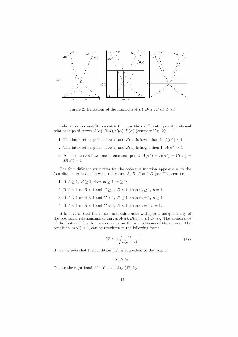
Figure 2: Behaviour of the functions A(α), B(α), C(α), D(α)
Taking into account Statement 4, there are three different types of positionalrelationships of curves A(α), B(α), C(α), D(α) (compare Fig. 2):
1. The intersection point of A(α) and B(α) is lower than 1: A(α∗) < 1
2. The intersection point of A(α) and B(α) is larger then 1: A(α∗) > 1
3. All four curves have one intersection point: A(α∗) = B(α∗) = C(α∗) =D(α∗) = 1.
The four different structures for the objective function appear due to thefour distinct relations between the values A, B, C and D (see Theorem 1):
1. If A ≥ 1, B ≥ 1, then m ≥ 1, n ≥ 1;
2. If A < 1 or B < 1 and C ≥ 1, D < 1, then m ≥ 1, n = 1;
3. If A < 1 or B < 1 and C < 1, D ≥ 1, then m = 1, n ≥ 1;
4. If A < 1 or B < 1 and C < 1, D < 1, then m = 1 n = 1.
It is obvious that the second and third cases will appear independently ofthe positional relationships of curves A(α), B(α), C(α), D(α). The appearanceof the first and fourth cases depends on the intersections of the curves. Thecondition A(α∗) > 1, can be rewritten in the following form:
W > u
√rs
h(h+ u). (17)
It can be seen that the condition (17) is equivalent to the relation
α1 > α2.
Denote the right hand side of inequality (17) by:
12

W ∗ = u
√rs
h(h+ u).
If W > W ∗ there exists an interval when simultaneously A > 1 and B > 1:(α1, α2), this is the first case of theorem 1. Therefore,
m ≥ 1, n = 1, α ∈ (0, α1)
m ≥ 1, n ≥ 1, α ∈ [α1, α2]
m = 1, n ≥ 1, α ∈ (α2, 1)
On the other hand, if W < W ∗, we obtain that at any α ∈ (0, 1) either A(α)or B(α) is less then one, here we have second, third and fourth cases of theorem1:
m ≥ 1, n = 1, α ∈ (0, α3]
m = 1, n = 1, α ∈ (α3, α4)
m = 1, n ≥ 1, α ∈ [α4, 1)
In the third situation, if W = W ∗, when the four curves have a commonunique intersection, α1 = α2 = α3 = α4 = α∗ = α∗∗, we have:
m ≥ 1, n = 1, α ∈ (0, α∗]
m = 1, n ≥ 1, α ∈ [α∗, 1)
Numerical example 1 Consider a case with the parameters d = 10000, h =5, u = 2, r = 30, s = 90, r1 = 50, s1 = 150. Consider different values ofparameter α ∈ (0, 1). Switching Costs: W = 80.
It can be easily calculated that A(α∗) = 4, 55 and W ∗ = 17, 57. Herewe have the appearance of the first case of Theorem 1. We find that: α1 =0, 31, α2 = 0, 903. Consider also the case when all parameters are the same butthere is no switching cost in consideration, i.e., W = 0. Denote by K(m,n, α)the corresponding cost. For the results see Fig. 3.
Numerical example 2 Consider a case with parameters: d = 10000, h =5, u = 2, r = 30, s = 90, r1 = 32, s1 = 93. Consider different values ofparameter α ∈ (0, 1). Switching Costs W = 5. A(α∗) = 0, 29. W ∗ = 17, 57.We have that W ∗ > W and then find α3 = 0, 657, α4 = 0, 713. The results aredisplayed in Fig. 4.
6 The optimal waste disposal rate (problem OWDR)
In this section the problem OWDR is considered. Let α ∈ [0, 1]. Note that onthe one hand, in some situations no remanufacturing is suitable. In this case
13

α = 1, m = 0, n = 1, and the model reduces to the classical EOQ:
KEOQα=1 (x) =
ds
x+
hx
2
with the optimal cost equal to√2dsh. On the other hand, if all products are
remanufactured, then α = 0, m = 1, n = 1 and the model would be:
KEOQα=0 (x) =
dr
x+
(h+ u)x
2
and the optimal cost would be equal to√2dr(u+ h).
Recall that for all other α the functionK(m,n) was defined as (6): K(m,n) =√2dL(m,n).Let us denote
K1 =√2dL1 =
√2d(√
Wa1 +√Ra2 +
√Sa3),
K2 =√2dL2 =
√2d(√
(W + S)(a1 + a3) +√Ra2),
K3 =√2dL3 =
√2d(√
(W +R)(a1 + a2) +√Sa3),
K4 =√2dL4 =
√2d(W +R+ S)(a1 + a2 + a3).
It can be easily proved that
K4 ≥ K2 ≥ K1,
K4 ≥ K3 ≥ K1.
Substituting the formulas (5) for the initial parameters gives
K1 =√2d(√Wαβu+ α
√sh+ β
√r(h+ u)) ≥
√2d(√
Wαβu+min{√sh,√r(h+ u)}) ≥ min{
√2dsh,
√2dr(h+ u)}.
We obtained that if α ∈ [0, 1], the optimal strategy for minimizing thetotal costs will be α = 1 and α = 0 with the costs
√2dsh or
√2dr(u+ h),
correspondingly. The case α ∈ [αmin, αmax], 0 < αmin ≤ α ≤ αmax < 1 will bestudied in the future.
7 Summary and conclusions
In this paper we analysed the extended EOQ repair and waste disposal modelwith switching costs. Two problems were considered: ONB and OWDR.
For the OWDR problem, we proved that the optimal strategy will be todispose of all used products or to remanufacture them all. This result agreeswith other results for similar problems.
We found the optimal policy P (m,n) for the ONB problem; it can have adifferent structure depending on the value of the parameters A,B,C,D. Theoptimal policy (m,n) depends on the disposal rate α, ceteris paribus; in other
14

words, the higher the α and the higher them, the lower the n. The impact of theswitching cost becomes apparent for sufficiently high values. In this case the op-timal numbers (m,n) can both be greater than one. This was illustrated by theexamples. To our knowledge, the case of having both optimal numbers m andn greater then one, if m remanufacturing batches are followed by the sequenceof n manufacturing batches or vice versa, has not been previously mentioned inthe literature. Choi et al. [4] found solutions with n and m both greater thanone, but they had placed the n manufacturing batches and m recovery batchesin different orders and considered the ordered sequence of manufacturing andremanufacturing batches within the cycle as decision variables. They found thatonly 0.2% of the 8,100,000 tested problems had an optimal solution with bothm and n greater then one. In this study we conducted a numerical analysis foran EOQ repair and waste disposal model with switching costs and we foundthat the optimal m and n are both greater then one in about 23% of 10,000different sets of parameters.
AcknowledgementsFirst author wish to thank Saint Petersburg State University for supporting
this research.
Appendix A
Lemma 1. If m > 0, n > 0, there are two curves of local minima (9) withrespect to m:
N(m) =
√a3m(W +mR)
S(a1m+ a2), (18)
with respect to n :
M(n) =
√a2n(W + nS)
R(a1n+ a3), (19)
and the point of local minimum:
(m∗, n∗) =
(√Wa2Ra1
,
√Wa3Sa1
). (20)
Proof. It follows from (10) that
∂L(m,n)
∂m< 0 ⇔ R(a1 +
a3n)− a2
m2(W + nS) < 0 ⇔ m < M(n).
In other words, the function L(m,n) decreases in m, if m < M(n) andincreases in m, if m > M(n).
∂2L
∂m2=
2a2(W + nS)
m3> 0,
15

if m > 0, n > 0. This means that L(m,n) is convex in m, therefore M(n) is thecurve of local minimum in m.
Substituting the expression for m (12) into (9) leads to
L(M(n), n) = 2
√a2R(Sn+W )(a1n+ a3)
n+ Sa1n+
Wa3n
+Ra2 + Sa3.
By differentiating L(M(n), n) with respect to n we receive
L′(M(n), n) =
(Sa1 −
Wa3n2
)(1 +
√Ra2n
(Sn+W )(a1n+ a3)
)
and as the result
m∗ =
√Wa2Ra1
, n∗ = N(m∗) =
√Wa3Sa1
.
Since the Hessian
D(m∗, n∗) =
∣∣∣∣∣ ∂2L∂m2
∂2L∂m∂n
∂2L∂n∂m
∂2L∂n2
∣∣∣∣∣(m∗,n∗)
=
(4a2a3W (W + nS +mR)
m3n3−
−(Ra3
n2− Sa2
m2
)2)(m∗,n∗)
=4a2a3W (W + n∗S +m∗R)
(m∗)3(n∗)3≥ 0
is positively definite matrix, (20) is the point of local minimum of the function(7).
Theorem 1. The optimal solution to the problem (9) has the following structuredepending on the value of the parameters A,B,C,D:
1. If A ≥ 1, B ≥ 1, then m =√A, n =
√B,
L = L1 = (√Wa1 +
√Ra2 +
√Sa3)
2
2. If A < 1 or B < 1 and C ≥ 1, D < 1, then m =√C, n = 1,
L = L2 = (√(W + S)(a1 + a3) +
√Ra2)
2
3. If A < 1 or B < 1 and C < 1, D ≥ 1, then m = 1, n =√D,
L = L3 = (√(W +R)(a1 + a2) +
√Sa3)
2
4. If A < 1 or B < 1 and C < 1, D < 1, then m = 1 n = 1,L = L4 = (W +R+ S)(a1 + a2 + a3)
Proof. The outline of the proof:
1. To find the optimal (m,n) using the Kuhn–Tucker conditions supposingL(m,n) to be the convex function.
2. To prove that the function L(m,n) is convex at least at the point (m∗, n∗).
16

3. To prove that the function L(m,n) is quasi convex at m > 0, n > 0.
4. To prove that the (m,n) which satisfies the Kuhn–Tucker conditions isoptimal using quasi convexity of L(m,n) and the Arrow and Enthoven,1961 [3] theorem.
5. To find the values L1, L2, L3, L4
1. Recall that
A =Wa2Ra1
B =Wa3Sa1
C =a2(S +W )
R(a1 + a3)
D =a3(W +R)
S(a1 + a2).
Let function L(m,n) be the convex function, then the Kuhn–Tucker con-ditions for problem (9) are as follows:
R(a1 +a3n)− a2
m2(W + nS)− λ1 = 0
S(a1 +a2m
)− a3n2
(W +mR)− λ2 = 0
m− 1 ≥ 0
n− 1 ≥ 0
λ1(m− 1) = 0
λ2(n− 1) = 0
λ1 ≥ 0, λ2 ≥ 0.
(21)
Let us denote
λ1(m,n) = R(a1 +a3n)− a2
m2(W + nS),
λ2(m,n) = S(a1 +a2m
)− a3n2
(W +mR).(22)
Recall that a2 > 0, a3 > 0. The condition λ1(1, 1) > 0 is equivalent tothe condition C < 1 and similarly λ2(1, 1) > 0 ⇔ D < 1. If λ1(1, 1) >0(⇔ C < 1) and λ2(1, 1) > 0(⇔ D < 1) then
m = 1
n = 1
λ1 = λ1(1, 1) > 0
λ2 = λ2(1, 1) > 0
17

satisfy the Kuhn–Tucker conditions (21). If λ1(1, 1) > 0(⇔ C < 1) andλ2(1, 1) ≤ 0(⇔ D ≥ 1) then consider
λ1(1,√D) = (Ra1 −Wa2)(1 +
S
W +R
√D).
If Ra1 −Wa2 > 0(⇔ A < 1) thenm = 1
n = N(1) =√D
λ1 = λ1(1,√D) > 0
λ2 = 0
satisfy the Kuhn–Tucker conditions (21). If Ra1 − Wa2 < 0(⇔ A > 1)then {
C < 1
A > 1⇔
(Wa2 −Ra1)︸ ︷︷ ︸
>0
+(Sa2 −Ra3) < 0
A > 1
⇒
{Sa2 −Ra3 < 0
A > 1⇔
{AB < 1
A > 1⇒ 1 < A < B ⇒ B > 1
which means that m =
√A
n =√B
λ1 = λ1(√A,
√B) = 0
λ2 = λ1(√A,
√B) = 0
satisfy the Kuhn–Tucker conditions (21). In the same way, if If λ1(1, 1) ≤0(⇔ C ≥ 1) and λ2(1, 1) ≤ 0(⇔ D ≥ 1) then Let Sa2 −Ra3 > 0 then{
D ≥ 1
Sa2 −Ra3 > 0⇔
(Wa3 − Sa1)− (Sa2 −Ra3)︸ ︷︷ ︸
>0
≥ 0
A > B
⇒
{Wa3 − Sa1 ≥ 0
A > B⇒
{B ≥ 1
A > B⇒
{A ≥ 1
B ≥ 1.
Let Sa2 −Ra3 < 0 then{C ≥ 1
Sa2 −Ra3 < 0⇔
(Wa2 −Ra1) + (Sa2 −Ra3)︸ ︷︷ ︸
<0
≥ 0
A < B
⇒
{Wa2 −Ra1 ≥ 0
A < B⇒
{A ≥ 1
A < B⇒
{A ≥ 1
B ≥ 1.
18

In any case m =
√A
n =√B
λ1 = λ1(√A,
√B) = 0
λ2 = λ1(√A,
√B) = 0
satisfy the Kuhn–Tucker conditions (21). We obtain that
• If C < 1, D < 1 then m = 1, n = 1
• If C < 1, D ≥ 1 then
– If A < 1, then m = 1, n =√D
– If A ≥ 1, then B ≥ 1 and m =√A,n =
√B
• If C ≥ 1, D > 1 then
– If B < 1, then m =√C, n = 1
– If B ≥ 1, then A ≥ 1 and m =√A,=
√B
• If C ≥ 1, D ≥ 1 then A ≥ 1, B ≥ 1 and m =√A,n =
√B.
2. Consider now concavity of the function L(m,n). As a result we have:
∂2L
∂m2=
2a2(W + nS)
m3> 0,
∂2L
∂n2=
2a3(W +mR)
n3> 0.
D(m,n) =
∣∣∣∣∣ ∂2L∂m2
∂2L∂m∂n
∂2L∂n∂m
∂2L∂n2
∣∣∣∣∣ = 4a2a3W (W + nS +mR)
m3n3−(Ra3
n2−Sa2
m2
)2≥ 0
at point (m∗, n∗) = (√
Wa2
Ra1,√
Wa3
Sa1) and at some epsilon neighborhood
of this point. It means that L(m,n) is concave at least at some epsilonneighborhood of (m∗, n∗).
3. Now we prove that L(m,n) is quasi convex. Bordered Hessians are equalto
B1(m,n) =
∣∣∣∣ 0 ∂L∂m
∂L∂m
∂2L∂m2
∣∣∣∣ = −(∂L
∂m
)2
≤ 0
B2(m,n) =
∣∣∣∣∣∣0 ∂L
∂m∂L∂n
∂L∂m
∂2L∂m2
∂2L∂m∂n
∂L∂n
∂2L∂n∂m
∂2L∂n2
∣∣∣∣∣∣ = −(∂L
∂m
)22a3(W +mR)
n3−
−(∂L
∂n
)22a2(W + nS)
m3− 2
∂L
∂m
∂L
∂n
(Ra3n2
+Sa2m2
)= −2(W + nS +mR)·
·
(a1
(Ra3n2
− Sa2m2
)2
+a2m
(Sa1m
− Wa3mn2
)2
+a3n
(Ra1n
− Wa2nm2
)2)
< 0,
19

if m = m∗, n = n∗. But at (m∗, n∗) the function L(m,n) is convex. Thismeans that L(m,n) is quasi convex at m > 0, n > 0.
4. And now we verify conditions from the following theorem: Theorem, Ar-row and Enthoven, 1961[3]. Let f(x) be a differentiable quasi-convex func-tion of the n-dimensional vector x, and let g(x) be an m-dimensional dif-ferentiable quasi-convex vector function, both defined for x0. Let x0 and λ0
satisfy the Kuhn–Tucker–Lagrange conditions, and let one of the followingconditions be satisfied:
a) fxi0> 0 for at least one variable xi0 ;
b) fxi1< 0 for some relevant variable xi1 ;
c) fx = 0 and f(x) is twice differentiable in the neighborhood of x0;
d) f(x) is convex.
then x0 minimizes f(x) subject to the constraints g(x) ≤ 0, x > 0. Ifm∗ ≥ 1, n∗ ≥ 1 then (m∗, n∗) satisfies (21) with λ1 = 0, λ2 = 0. The
condition d) is fulfilled. If m∗ ≥ 1, n∗ < 1 then (√
a2(W+S)R(a1+a3)
, 1) satisfies
(21) with λ1 = 0, λ2 > 0. The condition a) is fulfilled: λ2(√C, 1) = ∂L
∂n >0. Let m∗ < 1, n∗ < 1 and λ1(1, 1) ≥ 0, λ2(1, 1) ≥ 0 then m = 1, n = 1.The condition c) is fulfilled.
5. Substituting (√A,
√B) into L(m,n) we obtain:
L(√A,
√B) =
√2d(√Wa1 +
√Ra2 +
√Sa3) = L2
and in the same way
L(1, 1) =√2d(W +R+ S)(a1 + a2 + a3) = L3
L(√C, 1) =
√2d(√(W + S)(a1 + a3) +
√Ra2) = L1
L(1,√D) =
√2d(√(W +R)(a1 + a2) +
√Sa3) = L4
Appendix B
Property 1. The functions A(α), C(α) are positive and decreasing; if α ∈(0, 1), the functions B(α), D(α) are positive and increasing, if α ∈ (0, 1).
Proof. The functions A(α) and B(α) are obviously positive at any α ∈ (0, 1).The function A(α) is decreasing on (0, 1), if for any α ∈ (0, 1) : A′(α) < 0. Thelatest is true:
A′(α) = −W (h+ u)
ru
1
α2< 0, α ∈ (0, 1).
20

It can be shown in the same way that B′(α) > 0, if α ∈ (0, 1). Hence B(α) in-creases on (0, 1). To prove that C(α) is positive on (0, 1) consider the inequalityC(α) > 0. Let u > h then u
u−h > 1. Then C(α) > 0, if α ∈ (0, 1)∪(1, uu−h ). Let
u < h then uu−h < 0. Then C(α) > 0, if α ∈ (−∞, u
u−h ) ∪ (0, 1) ∪ (0,+∞). Inboth cases C(α) > 0 on (0, 1). To prove C(α) decreases, consider the inequalityC ′(α) < 0 we obtain:
(W + s)(h+ u)
r
(α− 1)(u+ α(2h− u))
α2(u+ α(h− u))2< 0.
There are three cases: if u > 2h then α ∈ (−∞, 0) ∪ (0, 1) ∪ ( uu−2h ,
uu−h ) ∪
( uu−h ,+∞), if 2h > u > h then α ∈ ( u
u−2h , 0) ∪ (0, 1), if h > u then α ∈( uu−2h , 0) ∪ (0, 1). In any case C ′(α) < 0 on (0, 1). This means that C(α)
decreases on (0, 1). It can be shown in the same way that D(α) is positive andthe derivative
D′(α) =(W + r)h
s
α(2(u+ h)− α(u+ 2h))
(1− α)2(u+ h− αh)2> 0
at any α ∈ (0, 1). Hence D(α) increases on (0, 1).
Property 2. Each of the equations A(α) = 1, B(α) = 1, C(α) = 1, D(α) = 1has a unique solution α1, α2, α3, α4, correspondingly, if α ∈ (0, 1):
α1 =W (h+ u)
ru+W (h+ u),
α2 =su
su+Wh,
α3 =
{12
2(W+s)(h+u)+ru−√
4hr(W+s)(h+u)+r2u2
(W+s)(h+u)−r(h−u) , (W + s)(h+ u)− r(h− u) = 0h−u2h+u , (W + s)(h+ u)− r(h− u) = 0
,
α4 =
{12
−s(u+2h)+√
4hs(W+r)(h+u)+u2s2
h(W+r−s) , W + r − s = 0u+hu+2h , W + r − s = 0
.
Proof. The proof is simply to prove that α1 is the unique solution of the equationA(α) = 1 and α2 is the unique solution of the equation B(α) = 1. Consider theequation C(α) = 1. It is equivalent to:
((W + s)(h+ u)− r(h− u))α2 − (2(W + s)(h+ u) + ru)α+ (W + s)(h+ u))
rα(u+ α(h− u))= 0.
If (W + s)(h+ u)− r(h− u) = 0, the numerator has two roots:
α13 =
1
2
2(W + s)(h+ u) + ru+√4hr(W + s)(h+ u) + r2u2
(W + s)(h+ u)− r(h− u),
α23 =
1
2
2(W + s)(h+ u) + ru−√4hr(W + s)(h+ u) + r2u2
(W + s)(h+ u)− r(h− u).
21

We simply show that if (W + s)(h + u) − r(h − u) > 0 then α13 > 1 and if
(W + s)(h+ u)− r(h− u) < 0 then α13 < 0. Regardless of whether (W + s)(h+
u)−r(h−u) is positive or not, α23 ∈ (0, 1). If (W +s)(h+u)−r(h−u) = 0 then
the numerator has the unique solution α03 = h−u
2h+u . It is obvious that α03 < 1. It
is necessary to prove that α03 > 0. From (W + s)(h+u)− r(h−u) = 0 it follows
that u = W+s−rW+s+rh < h. Hence α0
3 > 0, which is our proof. The denominatorhas two roots α = 0 and α = u
u−h . Neither root is in interval (0, 1). Thus itwas proved that the equation C(α) = 1 has a unique solution on (0, 1), whichis equal to
α3 =
{12
2(W+s)(h+u)+ru−√
4hr(W+s)(h+u)+r2u2
(W+s)(h+u)−r(h−u) , (W + s)(h+ u)− r(h− u) = 0h−u2h+u , (W + s)(h+ u)− r(h− u) = 0
.
The roots of the equation D(α) = 1 can be found in the same way.
Property 3. The functions A(α) and C(α) have two common points, if α ∈(0, 1]: (1, 0) and (α2,
W 2h(h+u)rsu2 ); moreover: A(α) ≥ C(α), if α ∈ [α2, 1], A(α) <
C(α), if α ∈ (0, α2). The functions B(α) and D(α) have two common points,
if α ∈ [0, 1): (0, 0) and (α1,W 2h(h+u)
rsu2 ); moreover: B(α) ≥ D(α), if α ∈ [0, α1],B(α) < D(α) if α ∈ (α1, 1).
Proof. According to Property 1, A(α) and C(α) are both decreasing functions.Consider the following inequality:
A(α) ≥ C(α) ⇔ (1− α)(α(us+ hW )− us)
uα(u+ α(h− u))≥ 0.
If u > h then α ∈ (−∞, 0)∪[ usus+hW , 1]∪( u
u−h ,+∞). If u < h then α ∈ ( uu−h , 0)∪
[ usus+hW , 1]. Hence, if α ∈ (0, 1) then A(α) ≥ C(α) on [ us
us+hW , 1] = [α2, 1], whichwas to be proved. This can be obtained in the same way as B(α) ≥ D(α), ifα ∈ [0, α1].
Property 4. The equations A(α) = B(α) and C(α) = D(α) have unique so-lutions α∗ and α∗∗, correspondingly. Moreover, if C(α∗∗) > 1 then A(α∗) > 1,if C(α∗∗) < 1 then A(α∗) < 1, if C(α∗∗) = 1 then A(α∗) = 1 and α∗ = α∗∗,where
α∗ =
√(h+u)s
ru
1 +√
(h+u)sru
A(α∗) = B(α∗) =W
u
√h(h+ u)
rs
(23)
Proof. Consider the following equation:
A(α) = B(α) (24)
22

It has a unique solution since A(α) is positive and monotonously decreasing andB(α) is positive and monotonously increasing for α ∈ (0, 1). Now, let α∗ be therate at which (24) holds. The value of α∗ is obviously equal
α∗ =
√(h+u)s
ru
1 +√
(h+u)sru
and is positive and less than one. Furthermore,
A(α∗) = B(α∗) =(s1 − s+ r1 − r)
u
√h(h+ u)
rs=
W
u
√h(h+ u)
rs.
Function C(α) is positive and monotonously decreasing for α ∈ (0, 1). SinceC(1) = 0 and limα→0 C(α) = +∞, then the range of values that the func-tion C(α) can take is an interval [0,+∞). D(α) is positive and monotonouslyincreasing for α ∈ (0, 1) with the range of values [0,+∞). This means thatequation C(α) = D(α) has a unique solution if α ∈ (0, 1) and curves C(α) andD(α) have one intersection point if α ∈ (0, 1). Recall that α = α∗ if (24) holds.Denote by α∗∗ the solution of C(α) = D(α), if α ∈ (0, 1). It can be proved thatif C(α∗∗) > 1 then A(α∗) > 1 and if C(α∗∗) < 1 then A(α∗) < 1. At first weprove that {
C ≥ 1
D ≥ 1⇒
{A ≥ 1
B ≥ 1.
For example, let Sa2 −Ra3 ≥ 0 ⇔ A > B then
C ≥ 1
D ≥ 1
A > B
⇔
(Wa2 −Ra1) + (Sa2 −Ra3)︸ ︷︷ ︸≥0
≥ 0
(Wa3 − Sa1)− (Sa2 −Ra3)︸ ︷︷ ︸≥0
≥ 0
A > B
⇒
{Wa3 − Sa1 > 0
A > B⇒
{B > 1
A > B⇒ A > B > 1.
It can be proved that if Sa2 − Ra3 < 0 then B > A > 1. In the same way itcan be proved that {
C < 1
D < 1⇒
{A < 1
B < 1.
We obtain that if at some α ∈ (0, 1), A(α) > 1 and B(α) > 1 then A(α∗) =B(α∗) > 1. If this is not so, for example A(α) > B(α) > 1 > A(α∗) =B(α∗), α∗ < α then A(α) and B(α) are both increasing functions, which is
23

not true. Consequently, if C(α∗∗) = D(α∗∗) > 1 then A(α∗) = B(α∗) > 1and if C(α∗∗) = D(α∗∗) < 1 then A(α∗) = B(α∗) < 1. Now to prove that ifC(α∗∗) = 1 then A(α∗) = 1. Let C(α∗∗) = 1 then at α = α∗:{
C = a2(S+W )R(a1+a3)
= 1
D = a3(W+R)S(a1+a2)
= 1.(25)
If a2S = a3R then from (25) it follows that{A = Wa2
Ra1= 1
B = Wa3
Sa1= 1.
If a2S > a3R then from (25) it follows that{A = Wa2
Ra1< 1
B = Wa3
Sa1> 1,
(26)
and from a2S > a3R it follows that A > B, which conflicts with (26). Thismeans that if α = α∗∗ then a2S = a3R, A = B = C = D = 1 and α∗ = α∗∗.
24

References
[1] AkcalıE., Cetinkaya S. (2011) Quantitative models for inventory and pro-duction planning in closed-loop supply chains. International Journal of Pro-duction Research 49(8): 2373–2407
[2] Andriolo A., Battini D., Grubbstromb R., Persona A., Sgarbossa F. (2014)A century of evolution from Harris’s basic lot size model: Survey and researchagenda. International Journal of Production Economics 155: 16–38
[3] Arrow K.J., Enthoven A.G. (1961) Quasi–Concave Programming. Econo-metrica, 29(4): 779–800
[4] Choi D.-W., Hwang H., Koh S.-G. (2007) A generalized ordering and re-covery policy for reusable items. European Journal of Operational Research182(2): 764–774
[5] Dobos I., Richter K. (2000) The integer EOQ repair and waste disposalmodel–further analysis. Central European Journal of Operations Research8(2): 173–194
[6] Dobos I., Richter K. (2003) A production/recycling model with stationarydemand and return rates. Central European Journal of Operations Research11(1): 35–46
[7] Dobos I., Richter K. (2004) An extended production/recycling model withstationary demand and return rates. International Journal of Production Eco-nomics 90(3): 311–323
[8] Dobos I., Richter K. (2006) A production/recycling model with quality con-sideration. International Journal of Production Economics 104(2): 571–579
[9] Hasanov P., Jaber M. Y., Zolfaghari S. (2012) Production remanufacturingand waste disposal model for a case of the cases of pure and partial backo-rdering. Applied Mathematical Modelling 36(11): 5249–5261
[10] Jaber M. Y., El Saadany A. M. A. (2009) The production, remanufactureand waste disposal model with lost sales. International Journal of ProductionEconomics120(1): 115–124
[11] Koh S.-G., Hwang H., Sohn K.-I. , Ko C.-S. (2002) An optimal orderingand recovery policy for reusable items. Computers and Industrial Engineering43: 59–73
[12] Kostantaras I. (2010) Optimal Control of Production and Remanufacturingin a Reverse Logistics Model with Backlogging. Mathematical Problems inEngineering. doi:10.1155/2010/320913
[13] Konstantaras I., Papachristos S. (2006) Lot-sizing for a single-product re-covery system with backordering. International Journal of Production Re-search 44(10): 2031–2045
25

[14] Konstantaras I., Papachristos S. (2008) A note on: Developing an exactsolution for an inventory system with product recovery. International Journalof Production Economics 111(2): 707–712
[15] Konstantaras I., Scouri K. (2010) Lot Sizing for a single product recov-ery system with variable setup numbers. European Journal of OperationalResearch 203(2): 326–335
[16] Konstantaras I., Scouri K., Jaber M.Y. (2010) Lot sizing for a recoverableproduct with inspection and sorting. Computer and Industrial Engineering58(3): 452–462
[17] Liu N., Kim Y., Hwang H. (2009) An optimal operating policy for theproduction system with rework. Computers and Industrial Engineering 56(3):874–887
[18] Mabini M. C., Pintelon L. M., Gelders L. F. (1992) EOQ type formula-tions for controlling repairable inventories. International Journal of Produc-tion Economics 28(1): 21–33
[19] Nahmias S., Rivera H. (1979) A deterministic model for a repairable iteminventory system with a finite repair rate. International Journal of ProductionResearch 17(3): 215–221
[20] Pishchulov G., Dobos I., Gobsch B., Pakhomova N., RichterK. A vendorpurchaser economic lot size problem with re-manufacturing // Journal of Business Economics, May 2014,http://link.springer.com/article/10.1007%2Fs11573-014-0731-7
[21] Richter K. (1996) The EOQ repair and waste disposal model with variablesetup numbers. European Journal of Operational Research 95(2): 313–324
[22] Richter K. (1996) The extended EOQ repair and waste disposal model.International Journal of Production Economics 45: 443–447
[23] Richter K. (1997) Pure and mixed strategies for the EOQ repair and wastedisposal problem. Operations-Research-Spektrum 19(2): 123–129
[24] Richter K., Dobos I. (1999) Analysis of the EOQ repair and waste disposalproblem with integer setup numbers. International Journal of ProductionEconomics 59: 463–467
[25] Rogers. D.S., Tibben-Lembke R.S. (1998) Going Backwards: Reverse Lo-gistics Trends and Practices. The University of Nevada, Reno, Center forLogistics Management, Executive Reverse logistics Council.
[26] El Saadany A. M. A., Jaber M. Y. (2008) The EOQ repair and wastedisposal model with switching costs. Computers and Industrial Engineering55(1): 219–233
26

[27] El Saadany A. M. A., Jaber M. Y. (2010) A production/remanufacturinginventory model with price and quality dependant return rate. Computersand Industrial Engineering 58(3): 352–362
[28] El Saadany A. M. A., Jaber M. Y., Bonney M. (2013) How many timesto remanufacture? International Journal of Production Economics 143(2):598–604
[29] Schrady D. A. (1967) A deterministic inventory model for reparable items.Naval Research Logistics Quarterly 14(3): 391–398
[30] Schulz T., Voigt G. (2014) A flexibly structured lot sizing heuristic for astatic remanufacturing system. Omega 44: 21-31
[31] Teunter R. H. (2001) Economic ordering quantities for recoverable iteminventory systems. Naval Research Logistics 48(6): 484–495
[32] Teunter R. H. (2004) Lot-sizing for inventory systems with product recov-ery. Computers and Industrial Engineering 46(3): 431–441
27

Figure 3: Example 1
Figure 4: Example 2
28