components of the assessment
TRANSCRIPT

UNIT 2
Components of the Assessment


CHAPTER 4
Overview of Assessment Problem Formulation
“If the Lord Almighty had consulted me before embarking on the Creation, I would have recommended something simpler.”
Alfonso X of Castile (Alfonso the Wise), 1221–1284
CONTENTS
Introduction ....................................................................................................................................102 Rationale for an Integrated Approach to Assessing Receiving Water Problems ................102
Watershed Indicators of Biological Receiving Water Problems ...................................................103 Summary of Assessment Tools ......................................................................................................107 Study Design Overview .................................................................................................................107 Beginning the Assessment .............................................................................................................108
Specific Study Objectives and Goals ...................................................................................110 Initial Site Assessment and Problem Identification .............................................................110 Review of Historical Site Data ............................................................................................112 Formulation of a Conceptual Framework ............................................................................113 Selecting Optimal Assessment Parameters (Endpoints) ......................................................113 Data Quality Objectives and Quality Assurance Issues ......................................................118
Example Outline of a Comprehensive Runoff Effect Study.........................................................119 Step 1. What’s the Question?...............................................................................................119 Step 2. Decide on Problem Formulation .............................................................................119 Step 3. Project Design..........................................................................................................120 Step 4. Project Implementation (Routine Initial Semiquantitative Survey)........................121 Step 5. Data Evaluation........................................................................................................122 Step 6. Confirmatory Assessment (Optional Tier 2 Testing) ..............................................122 Step 7. Project Conclusions .................................................................................................123
Case Studies of Previous Receiving Water Evaluations ...............................................................123 Example of a Longitudinal Experimental Design — Coyote Creek, San Jose, CA, Receiving Water Study .........................................................................................................124 Example of Parallel Creeks Experimental Design — Kelsey and Bear Creeks, Bellevue, WA, Receiving Water Study.................................................................................................139 Example of Long-Term Trend Experimental Design — Lake Rönningesjön, Sweden, Receiving Water Study .........................................................................................................169 Case Studies of Current, Ongoing, Stormwater Projects ....................................................181 Outlines of Hypothetical Case Studies ................................................................................205
101
102 STORMWATER EFFECTS HANDBOOK
Summary: Typical Recommended Study Plans ............................................................................213 Components of Typical Receiving Water Investigations .....................................................213 Example Receiving Water Investigations.............................................................................213
References ......................................................................................................................................218
INTRODUCTION
This chapter summarizes various approaches that have been used and recommended for evaluating receiving water effects. It outlines a reasonable method that allows the study designer to consider many factors that may affect the outcome of the project. Major study approaches are presented with extensive case study examples. The chapters and appendices in this book complement this material by providing guidance for developing an experimental design, methods for the collection of samples and their analysis, various other field evaluation efforts, and the statistical analysis of the data.
Rationale for an Integrated Approach to Assessing Receiving Water Problems
During the past decade, it has become apparent from numerous water and sediment quality assessment studies that no one single approach (e.g., chemical-specific criteria) can be routinely used to accurately determine or predict ecosystem health and beneficial use impairment. In Ohio, evaluation of indigenous biota showed that many of the impaired stream segments could not be detected using chemical criteria alone (EPA 1990b). In an intensive survey, 431 sites in Ohio were assessed using in-stream chemical and biological surveys. In 36% of the cases, chemical evaluations implied no impairment, but the biological survey evaluations did show impairment. In 58% of the cases the chemical and biological assessments agreed. Of these, 17% identified waters with no impairment, while 41% identified waters which were considered impaired. Realization of the inadequacy of nationwide criteria prompted the EPA to look for other site-specific criteria modifications. Numerous studies of bulk sediment contaminant concentrations failed to show significant correlations with toxic effects to test species (Burton 1991).
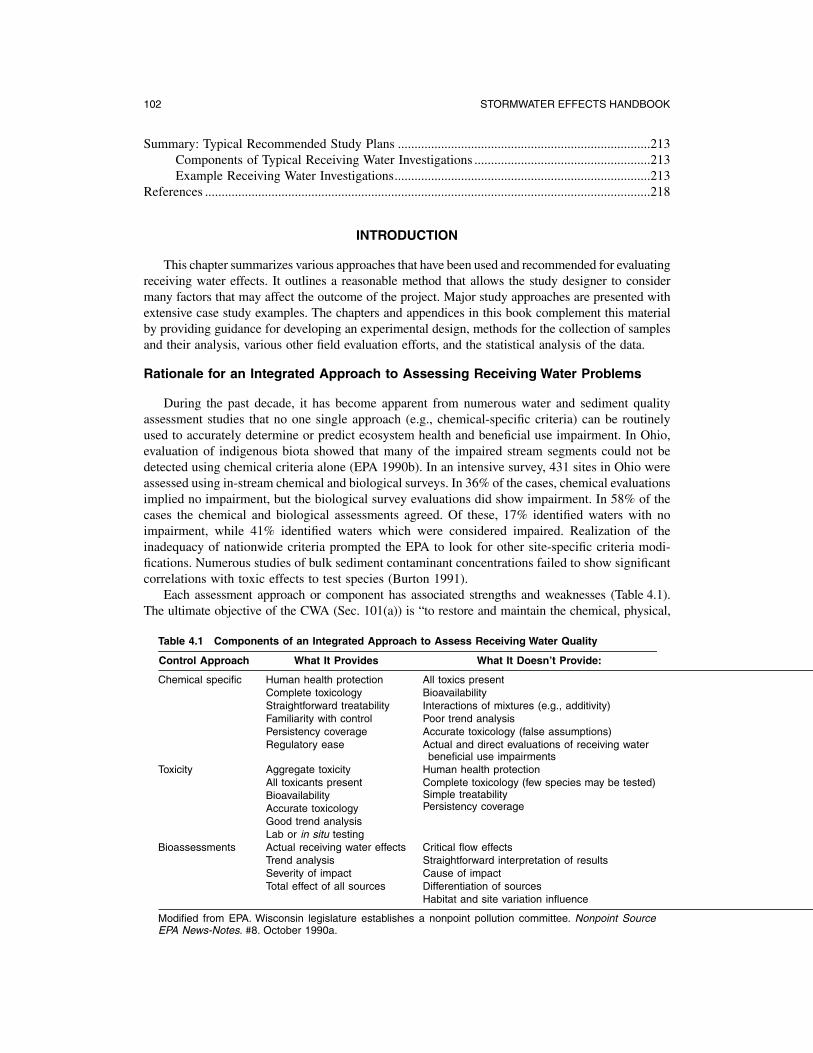
Each assessment approach or component has associated strengths and weaknesses (Table 4.1). The ultimate objective of the CWA (Sec. 101(a)) is “to restore and maintain the chemical, physical,
Table 4.1 Components of an Integrated Approach to Assess Receiving Water Quality
Control Approach What It Provides What It Doesn’t Provide:
Chemical specific Human health protection Complete toxicology Straightforward treatability Familiarity with control Persistency coverage Regulatory ease
Toxicity Aggregate toxicity All toxicants present Bioavailability Accurate toxicology Good trend analysis Lab or in situ testing
Bioassessments Actual receiving water effects Trend analysis Severity of impact Total effect of all sources
All toxics present Bioavailability Interactions of mixtures (e.g., additivity) Poor trend analysis Accurate toxicology (false assumptions) Actual and direct evaluations of receiving water beneficial use impairments
Human health protection Complete toxicology (few species may be tested) Simple treatability Persistency coverage
Critical flow effects Straightforward interpretation of results Cause of impact Differentiation of sources Habitat and site variation influence
Modified from EPA. Wisconsin legislature establishes a nonpoint pollution committee. Nonpoint Source EPA News-Notes. #8. October 1990a.

OVERVIEW OF ASSESSMENT PROBLEM FORMULATION 103
and biological integrity of the Nation’s waters.” These three components define the overall ecological integrity of an aquatic ecosystem (EPA 1990a). Pollutant loadings into receiving waters from point and nonpoint sources vary in magnitude, frequency, duration, and type. They are also strongly influenced by meteorological and hydrologic conditions, terrestrial processes, and land use activities.
A myriad of potential stressor combinations are possible in waters that are in human-dominated watersheds. In the laboratory, it would be impossible to evaluate even a small number of the possible stressor combinations, varying the magnitude, frequency, and duration of each stressor. Traditional bioassay methods simply look at one simple exposure scenario. Chemical criteria provide a benchmark from which to evaluate the significance of contaminant concentrations and direct further monitoring resources. Biological assessments indicate if the aquatic community is of a pollutionand/or habitat-tolerant or sensitive nature by showing the effect of long-term exposures. By considering habitat influence and comparing to reference sites, evaluations of ecological integrity (health) can be made. Habitat (physical) evaluations are essential to separate point source and nonpoint source toxicity effects from physical effects. As an example, some NPS pollution effects from stormwater may be of a physical nature, such as habitat alteration and destruction from increased stream flow, increased suspended and bedload sediments, or elevated water temperatures. In addition, a fourth major assessment component (toxicity) is needed beyond the three components of chemical, physical, and biological integrity (EPA 1990a). Biosurvey data may not detect subtle, short-term, or recent toxic effects due to the natural variation (spatial and temporal) that occurs in aquatic communities. Toxicity testing also removes the effects of habitat problems relatively well, focusing on the availability of chemical contaminants alone. The EPA (1990a) states that when any assessment approach (i.e., chemical-specific, toxicity, or biosurvey) shows water quality standards not being achieved, regulatory action should be taken.
The complexity of ecosystems dictates that these assessment tools be used in an integrated fashion. Scientists in any of the traditional disciplines (such as chemistry, microbiology, ecology, limnology, oceanography, hydrology, agronomy) are quick to point out the multitude of ecosystem complexities associated with their science. Many of these complexities influence chemical fate and effects and, more importantly, affect natural and anthropogenic stressor fate and effects. For example, it is well documented that many natural factors may act as significant stressors to organisms in aquatic systems, including light, temperature, flow, dissolved oxygen, sediment particle size, suspended solids, habitat quality, ammonia, salinity, food quality and quantity, predators, parasites, and pathogens. In addition, ecotoxicologists have long been aware of the differences between species and their life stages in regard to toxicant sensitivity. Unfortunately, toxicity information exists only for a fraction of the 1.5 to 100 million species (Wilson 1992; May 1994) and 7 million chemicals (U.S. General Accounting Office 1994) in the world. This reality makes extrapolations between species and chemicals tenuous at best. Despite these many and often interacting complexities, some excellent and proven tools exist for conducting ecologically relevant assessments of contamination.
The necessity of using each of the above assessment components and the degree to which each is utilized is a site-specific issue. At sites of extensive chemical pollution, extreme habitat destruction, or absence of desirable aquatic organisms, the impact can be clearly established with only one or two components, or simply qualitative measures. However, at most study sites, there will be “gray” areas where the ecosystem’s integrity (quality) is less clear and should be measured via multiple components, using a weight-of-evidence approach to evaluate adverse effects.
WATERSHED INDICATORS OF BIOLOGICAL RECEIVING WATER PROBLEMS
The EPA (1996) published a list of 18 indicators to track the health of the nation’s aquatic ecosystems. These indicators are intended to supplement conventional water quality analyses in compliance-monitoring activities. The use of broader indicators of environmental health is increasing. As an example, by 1996, 12 states were using biological indicators and 27 states were

104 STORMWATER EFFECTS HANDBOOK
developing local biological indicators, according to Pelley (1996). Because of the broad nature of the nation’s potential receiving water problems, this list is more general than typically used for any one specific discharge type (such as stormwater, municipal wastewaters, or industrial wastewaters). These 18 indicators are (EPA 1996):
1. Population served by drinking water systems violating health-based requirements 2. Population served by unfiltered surface water systems at risk from microbiological contamination 3. Population served by community drinking water systems exceeding lead action levels 4. Drinking water systems with source water protection programs 5. Fish consumption advisories 6. Shellfish-growing waters approved for harvest for human consumption 7. Biological integrity of rivers and estuaries 8. Species at risk of extinction 9. Rate of wetland acreage loss
10. Designated uses: drinking water supply, fish, and shellfish consumption, recreation, aquatic life 11. Groundwater pollutants (nitrates) 12. Surface water pollutants 13. Selected coastal surface water pollutants in shellfish 14. Estuarine eutrophication conditions 15. Contaminated sediments 16. Selected point source loadings to surface water and groundwater 17. Nonpoint source sediment loadings from cropland 18. Marine debris
In one example of the use of watershed indicators, Claytor (1996, 1997) summarized the approach developed by the Center for Watershed Protection as part of its EPA-sponsored research for assessing the effectiveness of stormwater management programs (Claytor and Brown 1996). The indicators selected are direct or indirect measurements of conditions or elements that indicate trends or responses of watershed conditions to stormwater management activities. Categories of these environmental indicators are shown in Table 4.2, ranging from conventional water quality measurements to citizen surveys. Biological and habitat categories are also represented. Table 4.3 lists 26 indicators, by category. It was recommended that appropriate indicators be selected from each category for a specific area under study. This will enable a better understanding of the linkage of what is done on the land, how the sources are regulated or managed, and the associated receiving water problems. The indicators were selected to (1) measure stress or the activities that lead to
Table 4.2 Stormwater Indicator Categories
Principal Element Being Category Description Assessed
Water quality Specific water quality characteristics Receiving water quality Physical/hydrologic Measure changes to, or impacts on, the Receiving water quality
physical environment Biological Use of biological communities to measure Receiving water quality
changes to, or impacts on, biological parameters
Social Responses to surveys or questionnaires to assess social concerns
Human activity on the land surface
Programmatic Quantify various nonaquatic parameters for measuring program activities
Regulatory compliance or program initiatives
Site Indicators adapted for assessing specific conditions at the site level
Human activity on the land surface
From Claytor, R.A. An introduction to stormwater indicators: urban runoff assessment tools. Presented at the Assessing the Cumulative Impacts of Watershed Development on Aquatic Ecosystems and Water Quality conference. March 20–21, 1996. Northeastern Illinois Planning Commission. pp. 217–224. Chicago, IL. April 1997.

OVERVIEW OF ASSESSMENT PROBLEM FORMULATION 105
Table 4.3 Environmental Indicators
Indicator Category Indicator Name
Water quality indicators
Physical and hydrologic indicators
Biological indicators
Social indicators
Programmatic indicators
Site indicators
Water quality pollutant constituent monitoring Toxicity testing Nonpoint source loadings Exceedance frequencies of water quality standards Sediment contamination Human health criteria Stream widening/downcutting Physical habitat monitoring Impacted dry-weather flows Increased flooding frequency Stream temperature monitoring Fish assemblage Macroinvertebrate assemblage Single species indicator Composite indicators Other biological indicators Public attitude surveys Industrial/commercial pollution prevention Public involvement and monitoring User perception Illicit connections identified/corrected BMPs installed, inspected, and maintained Permitting and compliance Growth and development BMP performance monitoring Industrial site compliance monitoring
From Claytor, R.A. An introduction to stormwater indicators: urban runoff assessment tools. Presented at the Assessing the Cumulative Impacts of Watershed Development on Aquatic Ecosystems and Water Quality conference. March 20–21, 1996. Northeastern Illinois Planning Commission. pp. 217–224. Chicago, IL. April 1997.
impacts on receiving waters, (2) assess the resource itself, and (3) measure the regulatory compliance or program initiatives. Claytor (1997) presented a framework for using stormwater indicators that is similar to many others recommended in hazard and risk assessment, as shown below:
Level 1 (Problem Identification): 1. Establish management sphere (who is responsible, other regulatory agencies involved, etc.). 2. Gather and review historical data. 3. Identify local uses that may be impacted by stormwater (flooding/drainage, biological integrity,
noncontact recreation, drinking water supply, contact recreation, and aquaculture). 4. Inventory resources and identify constraints (time frame, expertise, funding and labor
limitations). 5. Assess baseline conditions (use rapid assessment methods).
Obviously, the selection of the indicators to assess the baseline conditions should be based on the local uses of concern. Most of the anticipated important uses are shown to require indicators selected for each of the categories. However, the indicator selection process requires more than just a beneficial use consideration. Additional issues, such as the questions being asked, regulatory and societal concerns, the characteristics of the ecoregion, sensitive and threatened indigenous species, resource availability, and time constraints, are also important considerations.
Claytor (1997) also recommends a Level 2 assessment strategy for examining the local management program as outlined below:
106 STORMWATER EFFECTS HANDBOOK
Level 2: 1. State goals for program (based on baseline conditions, resources, and constraints) 2. Inventory prior and ongoing efforts (including evaluating the success of ongoing efforts) 3. Develop and implement management program 4. Develop and implement monitoring program (more quantitative indicators than typically used
for the Level 1 evaluations above) 5. Assess indicator results (does the stormwater indicator monitoring program measure the overall
watershed health?) 6. Reevaluate management program (update and revise management program based on measured
successes and failures)
While the approach and recommendations of Claytor (1997) have merit and provide a good overall framework, they may not adequately consider all the important study design issues for every specific area. Most important, their indicator guidance for determining receiving water effects from stormwater runoff may not provide a characterization of all the important stressors. For example, short-term pulses of polycyclic aromatic hydrocarbons from roadways and parking lots may be creating photoinduced toxicity problems not detected by traditional bioassessment approaches.
Another example of the effective use of environmental indicators is in the Detroit, MI, area. Cave (1998) described how they are being used to summarize the massive amounts of data being generated by the Rouge River National Wet Weather Demonstration Project in Wayne County. This large project is examining existing receiving water problems, the performance of stormwater and CSO management practices, and receiving water responses in a 438 mi2 watershed having more than 1.5 million people in 48 separate communities. The baseline monitoring program has now more than 4 years of continuous monitoring of flow, pH, temperature, conductivity, and DO, supplemented by automatic sampling for other water quality constituents, at 18 river stations. More than 60 projects are examining the effectiveness of stormwater management practices, and 20 projects are examining the effectiveness of CSO controls, each also generating large amounts of data. Toxicants are also being monitored in sediment, water, fish tissue, and with semipermeable membranes to help evaluate human health and aquatic life effects. Habitat surveys were conducted at 83 locations along more than 200 miles of waterway. Algal diversity and benthic macroinvertebrate assessments were also conducted at these survey locations. Electrofishing surveys were conducted at 36 locations along the main river and in tributaries. Several computer models were also used to predict sources, loadings, and wet-weather flow management options for the receiving waters and for the drainage systems. A geographic information system was used to manage and provide spatial analyses of the massive amounts of data collected. However, there was still a great need to simplify the presentation of the data and findings, especially for public presentations. Cave described how they developed a short list of 35 indicators, based on the list of 18 from EPA and on discussions with state and national regulatory personnel. They then developed seven indices that could be color-coded and placed on maps to indicate areas of existing problems and projected conditions based on alternative management scenarios. These indices are described as follows:
Condition Quality Indicators: 1. Dissolved oxygen. Concentration and % saturation values (ecologically important) 2. Fish consumption index. Based on advisories from the Michigan Department of Public Health 3. River flow. Significant for aquatic habitat and fish communities 4. Bacteria count. E. coli counts based on Michigan Water Quality Standards, distinguished for
wet and dry conditions
Multifactor Indices: 1. Aquatic biology index. Composite index based on fish and macroinvertebrate community
assessments (populations and individuals)
OVERVIEW OF ASSESSMENT PROBLEM FORMULATION 107
2. Aquatic habitat index. Habitat suitability index, based on substrate, cover, channel morphology, riparian/bank condition, and water quality
3. Aesthetic index. Based on water clarity, color, odor, and visible debris
These seven indicators represent 30 physical, chemical, and biological conditions that directly impact the local receiving water uses (water contact recreation, warm water fishery, and general aesthetics). Cave presented specific descriptions for each of the indices and gave examples of how they are color-coded for map presentation. These data presentations have clearly demonstrated how the Rouge River is degraded in specific areas and show the relationships of these critical river areas with adjacent watershed activities.
SUMMARY OF ASSESSMENT TOOLS
Almost all states using bioassessment tools have relied on the EPA reference documents as the basis for their programs. Common components of these bioassessment programs (in general order of popularity) include:
• Macroinvertebrate surveys (almost all programs, but with varying identification and sampling efforts)
• Habitat surveys (almost all programs) • Some simple water quality analyses • Some watershed characterizations • Few fish surveys • Limited sediment quality analyses • Limited stream flow analyses • Hardly any toxicity testing • Hardly any comprehensive water quality analyses
Normally, numerous metrics are used, typically only based on macroinvertebrate survey results, which are then assembled into a composite index. Many researchers have identified correlations between these composite index values and habitat conditions. Water quality analyses in many of these assessments are seldom comprehensive, a possible overreaction to conventional, very costly programs that have typically resulted in minimally worthwhile information. This book recommends a more balanced assessment approach, using toxicity testing and carefully selected water and sediment analyses to supplement the needed biological and habitat monitoring activities. A multicomponent assessment enables a more complete evaluation of causative factors and potential mitigation approaches.
STUDY DESIGN OVERVIEW
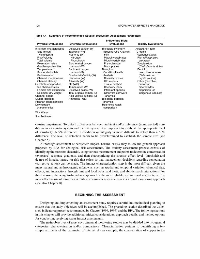
The study design must be developed based on the study objectives, preliminary site-problem assessments, regulatory mandates, and available resources. This chapter includes detailed information for developing the experimental design aspects of the study design. Many of the typical monitoring subcomponents of each approach are listed in Table 4.4. All of these parameters cannot realistically be evaluated in routine water quality assessments. The amount and type of monitoring hinges not only on the above issues but the degree of confidence and accuracy expected from the results. This issue falls under the Data Quality Objectives process and is also discussed in later chapters.
The most commonly used test hypotheses in assessing receiving water impacts is that the designated use or integrity of the water body is not impaired (null hypothesis), or the alternative hypotheses that it or some component is impaired or some specific factor (e.g., stormwater) is
108 STORMWATER EFFECTS HANDBOOK
Table 4.4 Summary of Recommended Aquatic Ecosystem Assessment Parameters
Indigenous Biota Physical Evaluations Chemical Evaluations Evaluations Toxicity Evaluations
In-stream characteristics Size (mean width/depth)
Flow/velocity Total volume Reaeration rates Gradient/pools/riffles Temperature Suspended solids Sedimentation Channel modifications Channel stability
Substrate composition and characteristics Particle size distribution Sediment dry weight
Channel debris Sludge deposits Riparian characteristics Downstream characteristics
Dissolved oxygen (W) Toxicants (WS) Nutrients (W)
Nitrogen Phosphorus
Biochemical oxygen demand (W)
Sediment oxygen demand (S)
Conductivity/salinity(W) Hardness (W) Alkalinity (W) pH (WS) Temperature (W) Dissolved solids (W) Total organic carbon (S) Acid volatile sulfides (S) Ammonia (WS)
Biological inventory (Existing Use Analysis): Fish Macroinvertebrates Microinvertebrates Phytoplankton Macrophytes
Biological Condition/Health Analysis: Diversity indices HIS models Tissue analysis Recovery index Intolerant species Omnivore-carnivore analysis
Biological potential analysis
Reference reach comparison
Acute/Short-term Chronic Responses(WS): Fish (Pimephales promelas)
Zooplankton (Ceriodaphnia dubia)
Benthic macroinvertebrates (Selenastrum capricornutum)
Other (microbial, protozoan, macrophytes, amphibian, or indigenous species)
W = Water
S = Sediment
causing impairment. To detect differences between ambient and/or reference (nonimpacted) conditions in an aquatic system and the test system, it is important to establish the appropriate level of sensitivity. A 5% difference in condition or integrity is more difficult to detect than a 50% difference. The level of detection needs to be predetermined to establish the sample size (see Chapter 5).
A thorough assessment of ecosystem impact, hazard, or risk may follow the general approach proposed by EPA for ecological risk assessments. The toxicity assessment process consists of identifying the stressors (hazards), using various measurement endpoints to determine concentration (exposure)–response gradients, and then characterizing the stressor–effect level (threshold) and degree of impact, hazard, or risk that exists so that management decisions regarding remediation (corrective action) can be made. The impact characterization step is the most difficult given the many natural and anthropogenic unknowns, such as spatial and temporal variation; chemical fate, effects, and interactions through time and food webs; and biotic and abiotic patch interactions. For these reasons, the weight-of-evidence approach is the most reliable, as discussed in Chapter 8. The most effective use of resources in routine stormwater assessments is via a tiered monitoring approach (see also Chapter 8).
BEGINNING THE ASSESSMENT
Designing and implementing an assessment study requires careful and methodical planning to ensure that the study objectives will be accomplished. The preceding section described the watershed indicator approach recommended by Claytor (1996, 1997) and the EPA. The following sections in this chapter will provide additional critical considerations, approach details, and method options for conducting receiving water impact assessments.
The main objectives of most environmental monitoring studies may be divided into two general categories: characterization and/or comparisons. Characterization pertains to quantifying a few simple attributes of the parameter of interest. As an example, the concentration of copper in the
OVERVIEW OF ASSESSMENT PROBLEM FORMULATION 109
sediment near an outfall may be of concern. The important question would be, “What is the most likely concentration of the copper?” Other questions of interest include changes in the copper concentrations between surface deposits and buried deposits, or in upstream vs. downstream locations. These additional questions are considered in the second category, namely, comparisons. Other comparison questions may relate to comparing the observed copper concentrations with criteria or standards. Finally, many researchers would also be interested in quantifying trends in the copper concentrations. This extends beyond the above comparison category, as trends usually consider more than just two locations or conditions. Examples of trend analyses would examine copper gradients along the receiving stream, or trends of copper concentrations with time. Another type of analysis related to comparisons is the identification of hot spots, where the gradient of concentrations in an area is used to identify areas having unusually high concentrations.
An adequate experimental design enables a researcher to efficiently investigate a study hypothesis. The results of the experiments will theoretically either prove or disprove the hypothesis. In reality, the experiments will tend to shed some light on the real problem and will probably result in many more questions that need addressing. In many cases, the real question may not have even been recognized initially. Therefore, even though it is very important to have a study hypothesis and appropriate experimental design, it may be important to reserve enough study resources to enable additional unanticipated experiments. In this discussion, sampling plans and specific statistical tools will be briefly examined.
Experimental design covers several aspects of a monitoring program. The most important aspect of an experimental design is being able to write down the study objectives and why the data are needed. The quality of the data (accuracy of the measurements) must also be known. Allowable errors need to be identified based on how the information will change a conclusion. Specifically, how sensitive are the data that are to be collected in defining the needed answer? A logical experimental process that can be used to set up an assessment of receiving waters consists of several steps:
1. Establish clear study objectives and goals (hypothesis to be tested, calibration of equation or model to be used, etc.).
2. Assess initial site assessment and identify preliminary problem. 3. Review historical site data. Collect information on the physical conditions of the system to be
studied (watershed characteristics, etc.), estimate the time and space variabilities of the parameters of interest (assumed, based on prior knowledge, or other methods).
4. Formulate a conceptual framework (e.g., the EPA ecological risk framework) and model. 5. Determine optimal assessment parameters. Determine the sampling plan (strata and relationships
that need to be defined), including the number of samples needed (when and where, within budget restraints).
6. Establish data quality objectives (DQO) and procedures needed for QA/QC during sample collection, processing, analysis, data management, and data analyses.
7. Locate sampling sites. 8. Establish field procedures, including the sampling specifics (volumes, bottle types, preservatives,
samplers to be used, etc.). 9. Review QA/QC issues.
10. Construct data analysis plan by determining the statistical procedures that will be used to analyze the data (including field data sheets and laboratory QA/QC plan).
11. Implement the study.
Preliminary project data obtained at the beginning of the project should be analyzed to verify assumptions used in the experimental design process. However, one needs to be cautious and not make major changes until sufficient data have been collected to verify new assumptions. After the data have been analyzed and evaluated, it is likely that follow-up monitoring should be conducted to address new concerns uncovered during the project.
110 STORMWATER EFFECTS HANDBOOK
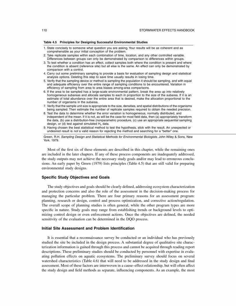
Table 4.5 Principles for Designing Successful Environmental Studies
1. State concisely to someone what question you are asking. Your results will be as coherent and as comprehensible as your initial conception of the problem.
2. Take replicate samples within each combination of time, location, and any other controlled variable. Differences between groups can only be demonstrated by comparison to differences within groups.
3. To test whether a condition has an effect, collect samples both where the condition is present and where the condition is absent (reference site) but all else is the same. An effect can only be demonstrated by comparison with a control.
4. Carry out some preliminary sampling to provide a basis for evaluation of sampling design and statistical analysis options. Deleting this step to save time usually results in losing time.
5. Verify that the sampling device or method is sampling the population it should be sampling, and with equal and adequate efficiency over the entire range of sampling conditions to be encountered. Variation in efficiency of sampling from area to area biases among-area comparisons.
6. If the area to be sampled has a large-scale environmental pattern, break the area up into relatively homogeneous subareas and allocate samples to each in proportion to the size of the subarea. If it is an estimate of total abundance over the entire area that is desired, make the allocation proportional to the number of organisms in the subarea.
7. Verify that the sample unit size is appropriate to the size, densities, and spatial distributions of the organisms being sampled. Then estimate the number of replicate samples required to obtain the needed precision.
8. Test the data to determine whether the error variation is homogeneous, normally distributed, and independent of the mean. If it is not, as will be the case for most field data, then (a) appropriately transform the data, (b) use a distribution-free (nonparametric procedure, (c) use an appropriate sequential sampling design, or (d) test against simulated H0 data.
9. Having chosen the best statistical method to test the hypothesis, stick with the result. An unexpected or undesired result is not a valid reason for rejecting the method and searching for a “better” one.
Green, R.H. Sampling Design and Statistical Methods for Environmental Biologists. John Wiley & Sons, New York. 1979.
Most of the first six of these elements are described in this chapter, while the remaining ones are included in the later chapters. If any of these process components are inadequately addressed, the study outputs may not achieve the necessary study goals and/or may lead to erroneous conclusions. An early paper by Green (1979) lists principles (Table 4.5) that are still valid for preparing environmental study designs.
Specific Study Objectives and Goals
The study objectives and goals should be clearly defined, addressing ecosystem characterization and protection concerns and also the role of the assessment in the decision-making process for managing the particular problem. There are four primary reasons for an assessment program: planning, research or design, control and process optimization, and corrective action/regulation. The overall scope of planning studies is often general, while the other program types are more specific in nature. Study goals may range from establishing trends or background levels to optimizing control design or even enforcement actions. Once the objectives are defined, the needed sensitivity of the evaluation can be determined in the DQO process.
Initial Site Assessment and Problem Identification
It is essential that a reconnaissance survey be conducted or an individual who has previously studied the site be included in the design process. A substantial degree of qualitative site characterization information is gained through this process and cannot be acquired through reading report descriptions. These preliminary studies should be conducted by personnel with expertise in evaluating pollution effects on aquatic ecosystems. The preliminary survey should focus on several watershed characteristics (Table 4.6) that will need to be addressed in the study design and final assessment. Most of these factors are interwoven in a cause–effect relationship, but will often affect the study design and field methods as separate, influencing components. As an example, the most

OVERVIEW OF ASSESSMENT PROBLEM FORMULATION 111
Table 4.6 Stream Assessment Factors for Nonpoint Source-Affected Streams
Watershed development factor
Best management practice
Hydrologic change factor
Channel form/stability factor
Substrate quality factor
Water quality factor
Stream community factor
Refugia factor
Riparian cover factor
Stream reach factor
Contiguous wetland factor
Floodplain change factor
Receiving water target factor
Imperviousness of contributing watershed and drainage efficiency of land use. Watershed area. Age of development. Nature of upstream land use. Percent forest cover. Pollutant (NPS and PS) input locations and dynamics.
Proportion of contributing watershed effectively controlled by a proposed BMP or retrofit. Type and performance of BMP.
Drainage efficiency (such as pre- vs. post-development runoff coefficients and times of concentrations). Dry-weather flow rate in modified vs. reference watershed. Frequent return period flows and associated channel dimensions.
Natural, eroded, open, lined, protected or enclosed channel form. Dry-weather wetted perimeter vs. reference watershed. Evidence of widening or downcutting. Bedrock controlled channel. Consolidated or unconsolidated banks. Channel gradient.
Median diameter or bed sediment. Degree of embeddedness. Reference substrate in undeveloped stream. Existing and future disturbed areas. Evidence of shifting sand bars, discolored cobbles.
Summer maximum temperature. Benthic algal growth. Organic slime on rocks. Silt and sand deposits in stream. Presence/absence of point source discharge or pipes along stream. Type and height of debris jams. Discolored or black rocks upon turning. Dry-weather water velocity.
Reference macroinvertebrate and fish species expected. Evidence of benthic algae or leaf processing. Rock turning or kick sampling. Cold, cool, or warm water community.
Presence of refuge habitats allowing species escape and reintroduction.
Presence or absence of riparian canopy cover over stream. Width of buffer 2 1/2 H max. Is vegetation stabilizing banks?
Presence or absence of pool and riffle structure. Minimum dryweather flow. Sinuosity of channel. Open or closed to fish migration. Creation of linear barrier across stream.
Presence or absence of nontidal wetlands in riparian, floodplain, or BMP zone. Quality, area, and function of wetlands present. Downstream wetlands to be affected?
Constrained or unconstrained floodplain. Extent of ultimate flood plain. Property in floodplain.
Are there any unique watershed water quality targets in a downstream river, lake, or estuary?
Modified from Schueler, T.R. Controlling Urban Runoff: A Practical Manual for Planning and Designing Urban BMPs. Department of Environmental Programs. Metropolitan Washington Council of Governments. Water Resources Planning Board. 1987.
important factors at the root of most nonpoint source pollution-related problems include watershed development characteristics whether of an urban, agricultural, or silviculture nature. Therefore, the preliminary problem identification process should begin with observations on the type, number, size, and location of point source discharges, stormwater inputs, upstream land use drainage patterns, and combined sewer overflows (CSOs).
A reference watershed should be located in the same type of ecoregion, but which has an undeveloped (unimpacted) watershed of a similar size with a stream (or lake) of a similar size. It is not practical to expect to find a completely natural and totally unimpacted watershed that can be used as a reference. The amount of allowable impact in the reference watershed will depend on the frequency and degree of exposure, persistence of the stressors, substrate composition, habitat and riparian quality, ecoregion and species sensitivity, and the range in water quality conditions.
The use of reference sites is common to most bioassessment approaches. Reference sites are typically selected to represent natural conditions as nearly as possible. However, it is not possible to identify such pristine locations representing varied habitat conditions in most areas of the country. Schueler (1997) points out that in many cases, a completely natural forested area is not a suitable

112 STORMWATER EFFECTS HANDBOOK
benchmark for current conditions before urbanization. In many areas of the country, land that has long been in agricultural use is being converted to urban land, and the in-stream changes expected should therefore be more reasonably compared to agricultural conditions.
The Ohio EPA has been recognized for having one of the more advanced biological assessments in place, especially in its efforts to incorporate biological criteria as part of the regulatory program. It relies heavily on a large network of reference sites representing the various ecological conditions throughout the state. Many of the states waterways were channelized decades ago. This severe habitat disruption prevents them from ever attaining as high a quality as a similar unchannelized waterway. Therefore, Ohio EPA established “modified” warm water habitat designations with appropriate modified reference sites. Few of these reference sites are completely unimpacted by modifications or human activity in the watersheds. Yoder and Rankin (1997) reported that biological monitoring of small streams in Ohio has indicated a general lowering of biological index scores with increasing urbanization, especially in areas having CSOs and industrial discharges. Of 110 sampling sites, only 23% had good to exceptional biological resources. Poor or very poor scores were evident in 85% of the urbanized areas. They also found that more than 40% of the suburban, urbanizing sites were impaired, due to increasing residential and commercial developments. An earlier Ohio study found that biological impairments were evident in about half the locations where no impairments were indicated, based on chemical ambient monitoring data alone. They have, therefore, come to rely on biological monitoring, such as expressed in the Index of Biotic Integrity (IBI) and the Invertebrate Community Index (ICI), as a less expensive and more accurate overall indication of receiving water problems than conventional chemical water pollutant monitoring.
Crawford and Lenat (1989) examined the differences between streams located in forested, agricultural, and urban watersheds in North Carolina. The USGS study found that the stream impacted by agricultural operations was intermediate in quality, with higher nutrient and worse substrate conditions than the urban stream, but better macroinvertebrate and fish conditions. The forested watershed had the best conditions (good conditions for all categories), except for somewhat higher heavy metal concentrations in sediment than expected. Even though the agricultural watershed had little impervious area, it had high sediment and nutrient discharges, plus some impacted stream corridors. The urban stream had poor macroinvertebrate and fish conditions, poor sediment and temperature conditions, and fair substrate and nutrient conditions.
Review of Historical Site Data
As in any environmental assessment process, historical site data should be reviewed initially. Municipal, county, regional, state, and federal information sources of public information may be available concerning:
1. Predevelopment water quality, fisheries, and flow conditions (e.g., state and EPA STORET database)
2. Annual hydrological conditions vs. development area (e.g., USGS) 3. Business and industrial categories (e.g., municipality) 4. Historical hazardous spills, large quantity toxicant releases and storage (e.g., fire department, state
EPA, and EPA’s Toxics Release Inventory), and hazardous waste and sanitary landfill locations (e.g., state and EPA)
The initial information search should review land use patterns from a chronological approach and attempt to correlate development with hydrological data and previous water quality surveys. Unfortunately, these data are often nonexistent for the small and more heavily impacted urban streams (headwaters). If the contaminants (stressors) of concern are known, site or area stream quality survey data can be used to determine the likely background levels in water, sediment, soil,
OVERVIEW OF ASSESSMENT PROBLEM FORMULATION 113
and fish. Also, one should determine what the effects and threshold levels are likely to be, and whether any rare, threatened, or endangered species are indigenous to the area. Sources of the above information may include state environmental and natural resource agencies; state game and fish agencies; conservation agencies; societies; citizens’ and sportsman’s groups; state agricultural agencies; relevant university departments; museums; park officials; local water and wastewater utilities; and regional offices of federal agencies (i.e., U.S. Fish and Wildlife Service, U.S. Environmental Protection Agency, U.S. Department of Agriculture, and Natural Resources Conservation Service). From this information, it is possible to determine which species are most likely to be present and what problems may exist in an area.
Formulation of a Conceptual Framework
A conceptual framework is similar to logistical critical-path control schedules, where the major components of the study (i.e., investigation of pollutant sources, hydrologic analyses, and stream and ecosystem monitoring) are blended to describe source movement, distribution, and interaction with the receiving water ecosystem. Once the previous steps are completed, it should be possible to formulate a suitable assessment problem formulation. This process is improved if there are adequate knowledge and expertise to address the key issues of pollutant types expected, predicted pollutant fate and effects, beneficial use designations, stream hydrological characteristics, meteorological characteristics, reference and test stream water quality, and key indicator aquatic organisms present at the reference and test locations. This design stage leads directly to the next step of defining measurement endpoints.
This process should be tailored toward addressing the study objectives. If the study is to be an “endangerment,” “hazard,” or “risk” assessment to meet EPA regulatory requirements (e.g., RCRA, CERCLA), it would be best to follow their assessment paradigm:
1. Hazard identification: qualitative stress (e.g., lead) and receptor (e.g., trout) identification 2. Exposure assessment: contaminant (stress) dynamics vs. receptor patterns and characteristics 3. Toxicity assessment: stress–response relationship quantified 4. Hazard or risk characterization: combine above information to predict or assign adverse effects
vs. source exposure
The specifics of these approaches are currently still under development by the EPA. This book could possibly be used to support any program directive which includes assessing the effects of stormwater runoff on receiving water ecosystems.
Selecting Optimal Assessment Parameters (Endpoints)
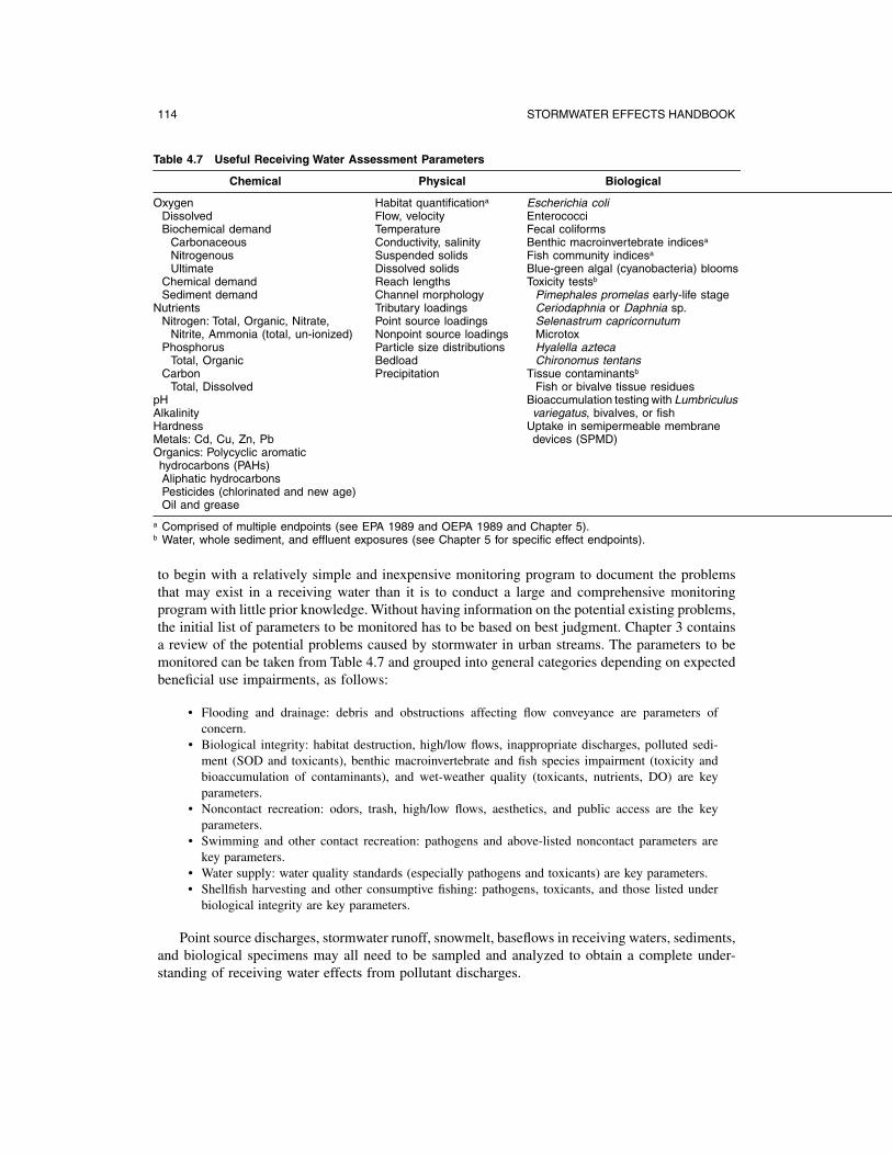
Characterization of the ecosystem should allow for differentiation of its present “natural” status from its present condition caused by polluted discharges and/or other anthropogenic stressors. This requires that a number of chemical, biological, and physical parameters be monitored, including flow and habitat. There are a wide variety of potentially useful study parameters which vary in importance with the study objectives and program needs, as shown in Table 4.7. Many of the chemical endpoints would be specifically selected based on the likely pollutant sources in the watershed. Those shown in Table 4.7 are a general list.
The selection of the specific endpoints for monitoring should be based on expected/known receiving water problems. The parameters being monitored should confirm if these uses are being impaired. If they are, then more detailed investigations can be conducted to understand the discharges of the problem pollutants, or the other factors, causing the documented problems. Finally, control programs can be designed, implemented, and monitored for success. Therefore, any receiving water investigation should proceed in stages if at all possible. It is much more cost-effective
114 STORMWATER EFFECTS HANDBOOK
Table 4.7 Useful Receiving Water Assessment Parameters
Chemical Physical Biological
Oxygen Dissolved Biochemical demand
Carbonaceous Nitrogenous Ultimate
Chemical demand Sediment demand
Nutrients Nitrogen: Total, Organic, Nitrate,
Nitrite, Ammonia (total, un-ionized) Phosphorus
Total, Organic Carbon
Total, Dissolved pH Alkalinity Hardness Metals: Cd, Cu, Zn, Pb Organics: Polycyclic aromatic hydrocarbons (PAHs) Aliphatic hydrocarbons Pesticides (chlorinated and new age) Oil and grease
Habitat quantificationa
Flow, velocity Temperature Conductivity, salinity Suspended solids Dissolved solids Reach lengths Channel morphology Tributary loadings Point source loadings Nonpoint source loadings Particle size distributions Bedload Precipitation
Escherichia coli Enterococci Fecal coliforms Benthic macroinvertebrate indicesa
Fish community indicesa
Blue-green algal (cyanobacteria) blooms Toxicity testsb
Pimephales promelas early-life stage Ceriodaphnia or Daphnia sp. Selenastrum capricornutum Microtox Hyalella azteca Chironomus tentans
Tissue contaminantsb
Fish or bivalve tissue residues Bioaccumulation testing with Lumbriculus variegatus, bivalves, or fish
Uptake in semipermeable membrane devices (SPMD)
a Comprised of multiple endpoints (see EPA 1989 and OEPA 1989 and Chapter 5). b Water, whole sediment, and effluent exposures (see Chapter 5 for specific effect endpoints).
to begin with a relatively simple and inexpensive monitoring program to document the problems that may exist in a receiving water than it is to conduct a large and comprehensive monitoring program with little prior knowledge. Without having information on the potential existing problems, the initial list of parameters to be monitored has to be based on best judgment. Chapter 3 contains a review of the potential problems caused by stormwater in urban streams. The parameters to be monitored can be taken from Table 4.7 and grouped into general categories depending on expected beneficial use impairments, as follows:
• Flooding and drainage: debris and obstructions affecting flow conveyance are parameters of concern.
• Biological integrity: habitat destruction, high/low flows, inappropriate discharges, polluted sediment (SOD and toxicants), benthic macroinvertebrate and fish species impairment (toxicity and bioaccumulation of contaminants), and wet-weather quality (toxicants, nutrients, DO) are key parameters.
• Noncontact recreation: odors, trash, high/low flows, aesthetics, and public access are the key parameters.
• Swimming and other contact recreation: pathogens and above-listed noncontact parameters are key parameters.
• Water supply: water quality standards (especially pathogens and toxicants) are key parameters. • Shellfish harvesting and other consumptive fishing: pathogens, toxicants, and those listed under
biological integrity are key parameters.
Point source discharges, stormwater runoff, snowmelt, baseflows in receiving waters, sediments, and biological specimens may all need to be sampled and analyzed to obtain a complete understanding of receiving water effects from pollutant discharges.
OVERVIEW OF ASSESSMENT PROBLEM FORMULATION 115
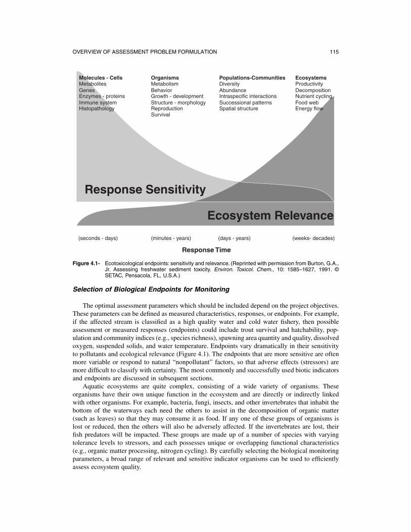
Molecules - Cells Metabolites Genes Enzymes - proteins Immune system Histopathology
Organisms Metabolism Behavior Growth - development Structure - morphology Reproduction Survival
Populations-Communities Diversity Abundance Intraspecific interactions Successional patterns Spatial structure
Ecosystems Productivity Decomposition Nutrient cycling Food web Energy flow
Response Sensitivity
Ecosystem Relevance
(seconds - days) (minutes - years) (days - years) (weeks- decades)
Response Time
Figure 4.1- Ecotoxicological endpoints: sensitivity and relevance. (Reprinted with permission from Burton, G.A., Jr. Assessing freshwater sediment toxicity. Environ. Toxicol. Chem., 10: 1585–1627, 1991. © SETAC, Pensacola, FL, U.S.A.)
Selection of Biological Endpoints for Monitoring
The optimal assessment parameters which should be included depend on the project objectives. These parameters can be defined as measured characteristics, responses, or endpoints. For example, if the affected stream is classified as a high quality water and cold water fishery, then possible assessment or measured responses (endpoints) could include trout survival and hatchability, population and community indices (e.g., species richness), spawning area quantity and quality, dissolved oxygen, suspended solids, and water temperature. Endpoints vary dramatically in their sensitivity to pollutants and ecological relevance (Figure 4.1). The endpoints that are more sensitive are often more variable or respond to natural “nonpollutant” factors, so that adverse effects (stressors) are more difficult to classify with certainty. The most commonly and successfully used biotic indicators and endpoints are discussed in subsequent sections.
Aquatic ecosystems are quite complex, consisting of a wide variety of organisms. These organisms have their own unique function in the ecosystem and are directly or indirectly linked with other organisms. For example, bacteria, fungi, insects, and other invertebrates that inhabit the bottom of the waterways each need the others to assist in the decomposition of organic matter (such as leaves) so that they may consume it as food. If any one of these groups of organisms is lost or reduced, then the others will also be adversely affected. If the invertebrates are lost, their fish predators will be impacted. These groups are made up of a number of species with varying tolerance levels to stressors, and each possesses unique or overlapping functional characteristics (e.g., organic matter processing, nitrogen cycling). By carefully selecting the biological monitoring parameters, a broad range of relevant and sensitive indicator organisms can be used to efficiently assess ecosystem quality.
116 STORMWATER EFFECTS HANDBOOK
The most commonly used biological groups in aquatic assessments are fish, benthic macroinvertebrates, zooplankton, and algae. In lotic (flowing water) systems, fish and benthic macroinvertebrates are often chosen as monitoring tools. Benthic refers to sediment or bottom surfaces (organic and inorganic). Macroinvertebrates are typically classified as those organisms which are retained in sieves larger than 0.3 to 0.5 mm. They include a wide range of invertebrates, such as worms, insect larvae, snails, and bivalves. They are excellent indicators of water quality because they are relatively sedentary and do not move between different parts of a stream or lake. In addition, a great deal is known about their life histories and pollution sensitivity. Algae, zooplankton, and fish are used more in lentic (lake) environments. Of these, fish are most often used (both in lotic and lentic habitats). Fish are transient, moving between sites, so it is more difficult to determine their source of exposure to stressors; however, they are excellent indicators of water quality and provide a direct link to human health and wildlife consumption advisories. Rooted macrophytes and terrestrial plant species are good wetland health indicators, but are used less frequently.
In order to effectively and accurately evaluate ecosystem integrity, biosurveys should use two to three types of organisms which have different roles in the ecosystem, such as decomposers (bacteria), producers, primary to tertiary consumers (EPA 1990b). This same approach should be used in toxicity testing (Burton et al. 1989, 1996; Burton 1991). This increases the power of the assessment, providing greater certainty that if there is a type of organism(s) (species, population, or community) in the ecosystem being adversely affected, either directly or indirectly, it will be detected. This also allows for better predictions of effects, such as in food chain bioaccumulation with subsequent risk to fish-eating organisms (e.g., birds, wildlife, humans). A large database exists for many useful indicator species concerning their life history, distribution, abundance in specific habitats or ecoregions, ecological function, and pollutant (stressor) sensitivity.
In the monitoring of fish and benthic macroinvertebrate communities, a wide variety of approaches have been used. A particularly popular approach recommended by the U.S. EPA, Ohio EPA, state volunteer monitoring programs, and other agencies is a multimetric approach, as summarized previously. The multimetric approach uses the basic data of which organisms are present at the site and analyzes the data using a number of different metrics, such as richness (number of species present), abundance (number of individuals present), and groups types of pollution-sensitive and resistant species. The various metrics provide unique and sometimes overlapping information on the quality of the aquatic community. Structural metrics describe the composition of a community, that is, the number and abundance of different species, with associated tolerance rankings. Functional metrics may measure photosynthesis, respiration, enzymatic activity, nutrient cycling, or proportions of feeding groups, such as omnivores, herbivores, insectivores, shredders, collectors, and grazers. The U.S. EPA and Ohio EPA approaches are described in more detail in Chapter 6 and Appendices A, B, and C.
The Microtox (from Azur) toxicity screening test has been successfully used in numerous studies to indicate the sources and variability of toxicant discharges. However, these tests have not been standardized by the U.S. EPA or state environmental agencies but have been in Europe. More typically, whole effluent toxicity test methods are employed (see Chapter 6, and also review by Burton et al. 2000). These tests may miss toxicant pulses and do not reflect real-world exposure dynamics. Many of the in situ toxicity tests, especially in conjunction with biological surveys (at least habitat and benthic macroinvertebrate evaluations) and sediment chemical analyses, can provide more useful information to document actual receiving water toxicity problems than relying on water analyses alone. If a water body is shown to have toxicant problems, it is best to conduct a toxicity identification evaluation (TIE) to attempt to isolate the specific problematic compounds (or groups of compounds) before long lists of toxicants are routinely analyzed.
Selection of Chemical Endpoints for Monitoring
An initial monitoring program must include parameters associated with the above beneficial uses. However, as the receiving water study progresses, it is likely that many locations and some
OVERVIEW OF ASSESSMENT PROBLEM FORMULATION 117
beneficial uses may not be found to be problematic. This would enable a reduction in the list of parameters to be routinely monitored. Similarly, additional problems may also become evident with time, possibly requiring an expansion of the monitoring program. The following paragraphs briefly describe the main chemical monitoring parameters that could be included for the beneficial use impact categories listed previously for a receiving water only affected by stormwater. However, it might be a good idea to periodically conduct a more-detailed analysis as a screening tool to observe less obvious, but persistent problems. If industrial or municipal point discharges or other nonpoint discharges (such as from agriculture, forestry, or mining activities) also affect the receiving water under study, additional constituents might need to be added to this list.
Obviously, chemical analyses can be very expensive. Therefore, care should be taken to select an appropriate list of parameters for monitoring. However, the appropriate number of samples must be collected (see Chapter 5) to ensure reliable conclusions. Chemical analyses of sediments may be more informative of many receiving water problems (especially related to toxicants) than chemical analyses of water samples. This is fortunate because sediment chemical characteristics do not change much with time, so generally fewer sediment samples need to be analyzed during a study period, compared to water samples. In addition, the concentrations of many of the constituents are much higher in sediment samples than in water samples, requiring less expensive methods for analyses. Unfortunately, sediment sample preparation (especially extractions for organic toxicant analyses and digestions for heavy metal analyses) can be much more difficult for sediments than for water.
Sediment Chemical Analyses
The basic list for chemical analyses for sediment samples, depending on beneficial use impairments, includes toxicants and sediment oxygen demand. The toxicants should include heavy metals (likely routine analyses for copper, zinc, lead, and cadmium, in addition to periodic ICP analyses for a broad list of metals). Acid volatile sulfides (AVS) are also sometimes analyzed to better understand the availability of the sediment heavy metals. Other sediment toxicant analyses may include PAHs and pesticides. Particle size analyses should also be routinely conducted on the sediment samples. Sediment oxygen demand analyses, in addition to an indication of sediment organic content (preferably particulate organic carbon, or at least COD and volatile solids), and nutrient analyses are important in areas having nutrient enrichment or oxygen depletion problems. Microorganisms (Escherichia coli, enterococci, and fecal coliforms) should also be evaluated in sediments in areas having likely pathogen problems (all urban areas). Interstitial water may also need to be periodically sampled and analyzed at important locations for the above constituents.
Water Chemical Analyses
The basic list for chemical analyses for water samples, depending on beneficial use impairments, includes toxicants, nutrients, solids, dissolved oxygen, and pathogens.
The list of specific toxicants is similar to that for the sediments (copper, zinc, lead, and cadmium, plus PAHs and pesticides). However, because of the generally lower concentrations of the constituents in the sample extracts for these analyses, more difficult analytical methods are generally needed, but the extraction and digestion processes are usually less complex than for sediments. In addition, because of the high variability of the constituent concentrations with time, many water samples are usually required to be analyzed for acceptable error levels. Therefore, less costly screening methods should be stressed for indicating toxicants in water. Because of the their strong associations with particulates, the toxicants should also be periodically analyzed in both their total and filterable forms. This increases the laboratory costs, but is necessary to understand the fates and controllability of the toxicant discharges. Typical chemical analyses for stormwater toxicants may include:
118 STORMWATER EFFECTS HANDBOOK
• Metals (lead, copper, cadmium, and zinc using graphite furnace atomic adsorption spectrophotometry, or other methods having comparable detection limits), periodic total and filtered sample analyses
• Organics (PAHs, phenols, and phthalate esters using GC/MSD with SIM, or HPLC), pesticides (using GC/ECD, or immunoassays), periodic total and filtered sample analyses
Pesticides in urban stormwater have recently started to receive more attention (USGS 1999). The USGS’s National Water Quality Assessment (NAWQA) program has extensively sampled urban and rural waters throughout the nation. Herbicides commonly detected in urban water samples include simazine, prometon, 2,4-D, diuron, and tebuthiuron. These herbicides are extensively used in urban areas. However, other herbicides frequently found in urban waters are used in agricultural areas almost exclusively (and likely drift in to urban lands from adjacent farm lands) and include atrazine, metolachlor, deethylatrazine, alachlor, cyanezine, and EPTC. Insecticides commonly detected in urban waters include diazinon, carbaryl, chlorpyrifos, and malathion.
Nutrient analyses are also important when evaluating several beneficial uses. These analyses are not as complex as the toxicants listed above and are therefore much less expensive. However, relatively large numbers of analyses are still required. Water analyses may include the following typical nutrients: total phosphorus, inorganic phosphates (and, by difference, organic phosphates), ammonia, Kjeldahl nitrogen (or the new HACH total nitrogen), nitrate plus nitrite, and TOC. Periodic analyses for total and filtered forms of the phosphorus and TOC should also be conducted.
Dissolved oxygen is a basic water quality parameter and is important for several beneficial uses. Historical discharge limits have typically been set based on expected DO conditions in the receiving water. The typical approach is to use a portable DO meter for grab analyses of DO. Continuous in situ monitors, described in Chapter 6, are much more useful, especially the new units that have much more stable DO monitoring capabilities and can also frequently record temperature, specific conductance, turbidity, pH, and ORP. These long-term analyses are especially useful when evaluating diurnal variations or storm-induced discharges.
Pathogens should be monitored frequently in most receiving waters. Both urban and rural streams are apparently much more contaminated by problematic pathogenic conditions than has previously been assumed. Historically monitored organisms (such as fecal coliforms), in addition to E. coli and enterococci which are now more commonly monitored, can be present at very high levels and be persistent in urban streams. Specific pathogens (such as Pseudomonas aeruginosa and Shigella) can also be more easily monitored now than in the past. Most monitoring efforts should probably focus on fecal coliforms, E. coli, and enterococci.
Additional conventional parameters affecting fates and effects of pollutants in receiving waters should also be routinely monitored, including hardness, alkalinity, pH, specific conductivity, COD, turbidity, suspended solids (SS), volatile suspended solids (VSS), and total dissolved solids (TDS).
Selection of Additional Endpoints Needed for Monitoring
Several other stream parameters also need to be evaluated when investigating beneficial uses. These may include debris and flow obstructions, high/low flow variations, inappropriate discharges, aesthetics (odors and trash), and public access.
Data Quality Objectives and Quality Assurance Issues
For each study parameter, the precision and accuracy needed to meet the project objectives should be defined. After this is accomplished, the procedures for monitoring and controlling data quality must be specific and incorporated within all aspects of the assessment, including sample collection, processing, analysis, data management, and statistical procedures (see also Chapter 7).
When designing a plan one should look at the study objectives and ask:

OVERVIEW OF ASSESSMENT PROBLEM FORMULATION 119
• How will the data be used to arrive at conclusions? • What will the resulting actions be? • What are the allowable errors?
This process establishes the Data Quality Objectives (DQOs), which determine the level of uncertainty that the manager is willing to accept in the results. DQOs, in theory, require the study designers (decision makers and technical staff) to decide what are allowable probabilities for Type I and II errors (false-positive and false-negative errors) and issues such as what difference in replicate means is significant. The DQO process is a pragmatic approach to environmental studies, where limited resources prevent the collection of data not essential to the decision-making process. Uncertainty in ecological impact assessments is natural due to variability and unknowns, sampling measurement errors, and data interpretation errors. Determining the degree of uncertainty in any of these areas can be difficult or impractical. Yet an understanding of these uncertainties and their relative magnitudes is critical to the QA objectives of producing meaningful, reliable, and representative data. The more traditional practices of QA/QC should be expanded to encompass these objectives and thus help achieve valid conclusions on the test ecosystem’s health (Burton 1992).
The first stage in developing DQOs requires the decision makers to determine what information is needed, reasons for the need, how it will be used, and to specify time and resource limits. During the second stage, the problem is clarified and constraints on data collection identified. The third stage develops alternative approaches to data selection, selecting the optimal approach, and establishing the DQOs (EPA 1984, 1986). Chapter 5 includes detailed information concerning the required sampling efforts to achieve the necessary DQOs, based on measured or estimated parameter variabilities and the uncertainty goals.
EXAMPLE OUTLINE OF A COMPREHENSIVE RUNOFF EFFECT STUDY
The following is an outline of the specific steps that generally need to be followed when designing and conducting a receiving water investigation. This outline includes the topics that are described in detail in later chapters of this book.
Step 1. What’s the Question?
For example: Does site runoff degrade the quality of the receiving-stream ecosystem? Chapter 3 is a summary of documented receiving water problems associated with urban stormwater, for example. That chapter will enable the investigator to identify the likely problems that may be occurring in local receiving waters, and to identify the likely causes.
Step 2. Decide on Problem Formulation
Candidate experimental designs can be organized in one of the following basic patterns:
1. Parallel watersheds (developed and undeveloped) 2. Upstream and downstream of a city 3. Long-term trend 4. Preferably, most elements of all of the above approaches combined in a staged approach
Examples of these problem formulations are included at the end of this chapter, while Chapter 5 describes basic study designs, such as stratified random sampling, cluster sampling, and search sampling.
Another important issue is determining the appropriate study duration. In most cases, at least 1 year should be planned in order to examine seasonal variations, but a longer duration may be

120 STORMWATER EFFECTS HANDBOOK
needed if unusual or dynamic conditions are present. As shown in Chapter 7, trend analyses can require many years. In addition, variations in the parameters being investigated will require specific numbers of observations in order to obtain the necessary levels of errors in the program (as described in Chapter 5). If the numbers of observations relate to events (such as runoff events), the study will need to last for the duration necessary to observe and monitor the required number of events.
Step 3. Project Design
1. Qualitative watershed characterization A. Establish degree of residential, commercial, and industrial area to predict potential stressors.
Typically, elevated solids, flows, and temperatures are stressors common to all urban land uses. The following lists typical problem pollutants that may be associated with each of these land uses: 1. Residential: nutrients, pesticides, fecal pathogens, PAHs, and metals 2. Commercial: petroleum compounds, metals 3. Industrial: petroleum compounds, other organics, metals 4. Construction: suspended solids
Topographical maps are used to determine watershed areas and drainage patterns. 2. Stream characterization
A. Identify potential upstream stressor sources and potential stressors 1. Photograph and describe sites.
B. Survey upstream and downstream (from outfall to 1 km minimum) quality. Record observations on physical characteristics, including channel morphology (pools, riffles, runs, modification), flow levels, habitat (for fish and benthos), riparian zone, sediment type, organic matter, oil sheens, and odors. Record observations on biological communities, such as waterfowl, fisheating birds or mammals, fish, benthic invertebrates, algal blooms, benthic algae, and filamentous bacteria.
C. Identify appropriate reference site upstream and/or in a similar sized watershed with same ecoregion.
D. Collect historical data on water quality and flows. 3. Select monitoring parameters
A. Habitat evaluation. Should be conducted at project initiation and termination. Includes Quantitative Habitat Evaluation Index (QHEI), bed instability survey (bed lining materials and channel cross-sectional area changes), aesthetic/litter survey, inappropriate discharges (field screening), etc.
B. Stressors and their indicators: 1. Physical: flow, temperature, turbidity. Determine at intervals throughout base to high flow
conditions. 2. Chemical: conductivity, dissolved oxygen, hardness, alkalinity, pH, nutrients (nitrates,
ammonia, orthophosphates), metals (cadmium, copper, lead, and zinc), and immunoassays (pesticides and polycyclic aromatic hydrocarbons) and/or toxicity screening (Microtox). The necessity of testing nutrients, metals, and organics will depend on the watershed characteristics. Determine at intervals throughout base to high flow conditions.
3. Biological: benthic community structure (e.g., RBP), fish community structure, and tissue residues (confirmatory studies only). Benthic structure should be determined at the end of the project. Sediment bioaccumulation potential can be determined using the benthic invertebrate Lumbriculus variegatus.
4. Toxicity: short-term chronic toxicity assays of stream water, outfalls, and sediment. Sediment should be sampled during baseflow conditions and tested before and after a high flow event. Water samples should be collected during baseflow and during pre-crest levels. Test species selection is discussed in Chapter 6 and in Appendix D. Expose test chambers with and without sunlight-simulating light (containing ultraviolet light wavelengths) to detect PAH toxicity. In situ toxicity assays should be deployed in the stream for confirmatory studies during base and high flow periods.
OVERVIEW OF ASSESSMENT PROBLEM FORMULATION 121
4. Data quality objectives. Determine the kinds of data needed and the levels of accuracy and precision necessary to meet the project objectives. These decisions must consider that there is typically a large amount of spatial and temporal variation associated with runoff study parameters. Chapter 5 relates sampling efforts associated with actual variability and accuracy and precision goals. This requires additional resources for adequate quantification.
5. Triggers and tiered testing. Establish the trigger levels or criteria that will be used to determine when there is a significant effect, when the objective has been answered, and/or when additional testing is required. Appropriate trigger levels may include: A. An arbitrary 20% difference in the test site sample, as compared to the reference site, might
constitute a significant effect. (However, as noted in Chapter 5, a difference this small for many parameters may be difficult and therefore expensive to detect because of the natural variability.)
B. An exceedance of the 95% statistical confidence intervals as compared to the reference sample. C. High toxicity in the test site sample, measured as Toxic Units (TUs) (e.g., 1/LC50). D. Exceedance of biotic integrity, sediment, or water quality criteria/guidelines/standards at the
test site E. Exceedance of a hazard quotient of 1 (e.g., site concentration/environmental effect or back
ground concentration). A tiered or a phased testing approach is most cost effective, if time permits. A qualitative or semiquantitative study may include a greater number of indicator or screening parameters, such as turbidity, temperature, DO, specific conductivity, and pH using a continuous recording water quality sonde, plus artificial substrate macroinvertebrate colonization tests, and “quick” sediment toxicity tests. If possible, Microtox screening toxicity tests, immunoassay tests for pesticides and PAHs, and sediment metal analyses should also be added to this initial effort. These simple tests can be conducted with more widespread sampling to better focus later tiers on quantifying appropriate stressors in critical sampling areas and times. Final project tiers can identify specific stressors, their contribution to the problem, their sources, or simply confirm the ecological significance of the observed effects.
6. Sampling station selection. Select the study sites, such as upstream reference sites, outfall(s), and downstream impacted sites. In the selection of the upstream/reference and downstream sites, consider flow dynamics, stressor sources, and reference habitat similarities.
7. Quality assurance project plans (QAPP). It is essential that the quality of the project be ensured with adequate quality assurance and quality control measures. This will include routine laboratory and field documentation of operator and instrumentation performance, chain-of-custody procedures, adequate sample replication, QA/QC samples (blanks and spikes, etc.), performance criteria, and ensuring data validity. Appropriate experimental design (study design and sampling efforts) is also a critical component of a QAPP.
Step 4. Project Implementation (Routine Initial Semiquantitative Survey)
1. Baseflow conditions A. Habitat survey (e.g., Qualitative Habitat Evaluation Index) B. Benthic RBP C. Test water and sediment from all test sites for short-term chronic toxicity with two species. D. Establish spatial and diurnal variation (YSI 6000 for several weeks, plus grab samples or time
composites). E. Set up automatic stream samplers/monitors, stream depth gauges, and rain gauges. F. Establish local contacts to oversee field equipment and provide rain event notification. G. Conduct field screening survey at outfalls to identify sources of dry-weather flows.
2. High flow conditions A. Confirm that the samplers and monitors are operational. Collect grab samples if necessary (for
microbiological and VOC analyses, for example). B. Deploy in situ toxicity test assays. C. Measure flow and note staff gauge depth, using manual or automatic samplers and flow
recorders. Repeat flow measurements at intervals of 0.5- to 1.0-ft stream depth intervals as the stream rises, noting time and depth. Focus on first flush to crest period.
122 STORMWATER EFFECTS HANDBOOK
D. Measure DO, temperature, turbidity, conductivity, and stage at each station following each flow measurement. Establish spatial variance. May use continuous recording water quality sondes.
E. Collect flow-weighted composited (or combine many discrete) samples for other analyses. 3. Sample analyses
A. Filter, preserve, and chill samples, as required. B. Deliver samples to analytical laboratories with chain-of-custody forms. C. Initiate toxicity testing and other chemical and microbiological analyses within required time
period since sample collection. D. Document QA/QC.
4. Follow-up (post-event) monitoring A. Check in situ assay chambers at 24 and 48 hours and at 7 and 14 days if deployed. B. Conduct benthic RBP. C. Conduct QHEI, noting bedload movement. D. Collect fish for tissue residue analyses.
Step 5. Data Evaluation
1. Plot flow vs. physical and chemical analysis results. 2. Statistically compare responses/loadings during base, first flush, and post-crest conditions. This
will provide a characterization of flow dynamics and its effect on stressor profiles. 3. Statistically compare stations (instantaneous, mean periods) for significant differences and corre
lations. 4. Calculate and compare physical, chemical, and toxicity (using Toxicity Units) loadings. This will
show the relative load contribution of stressors from reference (upstream) vs. impacted (downstream) reach.
5. Identify magnitude and duration of trigger exceedances. 6. Identify sources of uncertainty. 7. Identify potential sources of pollutants and stressors. 8. Determine literature value thresholds for key stressors on key indigenous species.
Step 6. Confirmatory Assessment (Optional Tier 2 Testing)
1. Repeat Steps 2 and 3 using Tier 1 information to select fewer test parameters with increased sampling frequency and/or select more descriptive methods. Increased sampling will better quantify the magnitude and duration of stressor dynamics. Expanded sampling will better document the quality of the receiving water. More definitive testing could include: A. Short-term chronic toxicity testing with additional species (lab and in situ) B. Increased testing of toxicants C. Characterizing fish, plankton, periphyton, or mussel populations D. Measuring assimilative capacity via long-term BOD and SOD testing E. Measuring productivity with light/dark bottle BOD in situ tests
2. Conduct toxicity identification evaluation (TIE) study of water, outfalls, and/or sediment to determine contribution of each stressor to total toxicity. This information can better determine which stressors are important to control and can also identify sources of toxicity.
3. Conduct bioaccumulation testing of site sediments. Some pollutants, such as highly chlorinated organic compounds (e.g., chlordane, DDT, PCBs, dioxins) are readily bioaccumulated, yet may not be detected using the above study design. The EPA has a benthic invertebrate 28-day assay to measure sediment bioaccumulation potential. Also SPMDs may be used.
4. Indigenous biological community characterization and tissue analysis. More in-depth quantification of benthic and/or fish community structure on a seasonal basis will better identify significant ecological effects. Tissue sampling of fish for contaminants will provide information on bioaccumulative pollutants and potential food web or human health effects from consumption.

OVERVIEW OF ASSESSMENT PROBLEM FORMULATION 123
Table 4.8 Watershed Study Complexity Matrix
Situation: Complexity Scale (Simple to Complex) Primary Considerations
Single outfall Small stream (small watershed)
Focus on loading of site stressors from site and from upstream. Reference upstream.
Large stream (larger watershed) Determine if upstream inputs are degrading water quality. Upstream and separate ideal reference sites.
Pristine estuary Focus on outfall quality and mixing zone. Deploy in situ monitors. Use far-field reference.
Multiple outfalls River (multi-watersheds) Multistation network with habitat, benthos, and select toxicity
evaluations of water and sediments.Tiered study with TIE, outfall, and in situ studies to find major problem sources. Use upstream and adjacent watershed references. Focus on tributary mouths for initial sampling and use SPMDs.
Coastal harbor Focus on outfall quality and near-field mixing zones. Deploy in situ monitors. Use far-field, adjacent watershed references.
Step 7. Project Conclusions
1. List probable stressors. 2. Document trigger exceedances. 3. Discuss relative contribution of stressors(s) to ecosystem degradation. Support documentation may
include: A. Literature threshold values B. Criteria exceedances C. Toxicity observed (from TIE, photoactivation, or in situ assays) D. Bioaccumulation factors and potential for food web contamination
4. Provide recommendations for stressor reduction and ecosystem enhancement. 5. Include suggestions on habitat improvement, flow reduction, turbidity removal, and reduced
siltation.
Table 4.8 summarizes the primary considerations that should be examined for different levels of receiving water complexity. Obviously, increasingly complex situations require more complex study designs and elements. However, this table briefly outlines the major issues that should be considered.
CASE STUDIES OF PREVIOUS RECEIVING WATER EVALUATIONS
This section presents several case studies that have been conducted to investigate receiving water problems associated with runoff. These case studies illustrate the major approaches used to identify a potentially affected area through comparisons with a control area. The basic experimental designs are:
• Above/below longitudinal study where a stream is studied as it flows from above a city through a city. Obviously, the upstream control reach must be in a relatively undisturbed portion of the watershed and only wet-weather flows of interest affect any of the test reaches.
• Parallel stream study where two (or more) streams are studied. One of the streams is a control stream in a relatively undisturbed area, while the other stream is in an urbanized area.
• Trend analyses with time in a single stream to investigate changes that may occur with time as a watershed becomes urbanized, or with the application of stormwater controls.
124 STORMWATER EFFECTS HANDBOOK
The selection of suitable test areas is critical. As noted, the control water body should be minimally affected by urbanization, while the urban test water body should be affected only by urban runoff (and not municipal or industrial discharges, for example) if possible. In addition, the test and control water bodies must be otherwise very similar (especially as watershed area, topography, habitat potential, etc., are concerned). In a longitudinal study, the watershed area obviously increases in a downstream (urbanized) direction. In addition, the urban water body has a substantially different flow regime than an undisturbed water body. These differences should be the result of urbanization and not other factors. A successful receiving water study usually requires several years of study at many locations in each stream segment. As noted throughout this book, the selection of monitoring parameters is also critical. In most cases, varied and complementary analyses should be conducted, covering a range of biological, physical, and chemical parameters. However, carefully designed investigations can be more successfully focused on limited project objectives.
The first three case studies are examples of these three basic experimental designs for conducting a receiving water investigation and include both test and control conditions. Most of the receiving water studies reported in the literature only focus on potentially impacted water bodies, without any adequate control sites. This may be suitable in an area where the receiving water potential is well understood through extensive prior studies (such as in Ohio). However, it is very problematic to rely solely on various criteria to identify the magnitude of receiving water problems, without extensive local expertise on relatively natural conditions.
The identification of a “problem” is also highly dependent on desired beneficial uses. The local perception of use is critical. Obviously, human health considerations associated with potentially contaminated water supplies, consumptive fisheries, or contact recreation areas must be stringently addressed. Biological uses may be more open to local interpretation, however. It is unreasonable to expect completely natural receiving water conditions in an urban area. There are unavoidable impacts that will prevent the best natural conditions from occurring in an urbanized watershed. Obviously, general biological uses can still be met by providing suitable habitat and somewhat degraded conditions that would allow a reasonable assemblage of aquatic organisms to exist in an area. Noncontact recreational uses (especially the aesthetic factors of odors and trash) should also be provided in urban receiving waters. Test and control receiving water investigations are very useful in that they enable contrasting of existing degraded conditions with less impacted conditions. Perhaps the control reference sites should include not natural conditions, but acceptable degraded conditions associated with partial urbanization. This is possible with a longitudinal study where a receiving water is studied as it flows through an urban area, becoming more degraded in the downstream direction. Parallel stream studies can also include partially degraded, but acceptable, sites. In addition, trend analyses with time will indicate when unacceptable degradation occurs.
Example of a Longitudinal Experimental Design — Coyote Creek, San Jose, CA, Receiving Water Study
The Coyote Creek study is an example of an investigation of the effects of stormwater on the biological conditions in an urban creek as it passed through the City of San Jose, CA. This was an early comprehensive receiving water study that examined many attributes of the creek above and within the city.
This research project included many different biological, chemical, and physical parameters to quantify biological effects. The project was conducted by Pitt and Bozeman (1982) from 1977 through 1982, with funding from the Storm and Combined Sewer Section of the U.S. Environmental Protection Agency. The objective of this 3-year field monitoring study was to evaluate the sources and impacts of urban runoff on water quality and biological conditions in Coyote Creek. In many cases, very pronounced gradients of water and biological quality indicators were observed. Cause-

OVERVIEW OF ASSESSMENT PROBLEM FORMULATION 125
and-effect relationships cannot be conclusively proven in a study such as this; the degradation of conditions in Coyote Creek may be due to several factors, including urban runoff, stream flows (both associated and not associated with urban runoff), and natural conditions (e.g., drought, stream gradient, groundwater infiltration, etc.). Information collected during this study implied that the effects of various urban runoff constituents, especially organics and heavy metals in the water and in the polluted sediment, may be responsible for many of the adverse biological conditions observed.
The beginning of the project followed 2 years of severe drought. The first major rains occurred the previous November (1977), and seasonal rains that occurred during the study period were considered normal. Typical rainfall averaged 33 cm (13 in) per year in the area below Lake Anderson, and 50 to 71 cm (20 to 28 in) per year in the watershed above Lake Anderson. During the drought, which preceded this study, rainfall was only about one half of these amounts.
Step 1. What’s the Question?
The major questions that were to be addressed during the Coyote Creek study were:
1. Identify and describe important sources of urban runoff pollutants. 2. Describe the effects of those pollutants on water quality, sediment quality, aquatic organisms, and
the creek’s associated beneficial uses. 3. Assess potential measures for controlling the problem pollutants in urban runoff.
Step 2. Decide on Problem Formulation
This project was designed to examine the changes in conditions in Coyote Creek as it passed through San Jose, CA. It was therefore a longitudinal study. The several-year duration of the study also enabled year-to-year variations to be compared to the differences in locations.
Step 3. Project Design
Qualitative Watershed Characterization
Figure 4.2 is a map of the San Francisco Bay area showing the location of the Coyote Creek watershed, while Figure 4.3 is a detailed map of the Coyote Creek watershed. The watershed itself is about 70 km (45 miles) long, 15 km (10 miles) wide, and contains about 80,000 ha (200,000 acres). Nearly 15% of the watershed consisted of developed urban areas during the study period. Most of the urban development is located in the northwest portion of the watershed.
Stream Characterization
For much of its length, Coyote Creek flows northwesterly along the western edge of the watershed. Elevations in the watershed range from sea level to nearly 920 m (3000 ft). Figure 4.4 shows the elevations of the various major sampling locations. Near the San Jose urban area, the watershed can be characterized as a broad plain with rolling foothills to the east. A portion of the watershed (i.e., the narrow strip between Lake Anderson and the urban area) is used for light but productive agriculture. The upper reaches and the headwaters of Coyote Creek are in extremely rugged terrain, with slopes commonly exceeding 30%. These upper areas can be characterized as chaparral-covered hills and gullies in a fairly natural state; they receive little use by man. Much of this land is within the Henry Coe State Park; non-park land is used primarily for low-density cattle grazing. Even though the watershed is very large and has upstream dams, the flow variations are extreme. Figure 4.5 shows the creek during a wet-weather period where the flows are overtopping
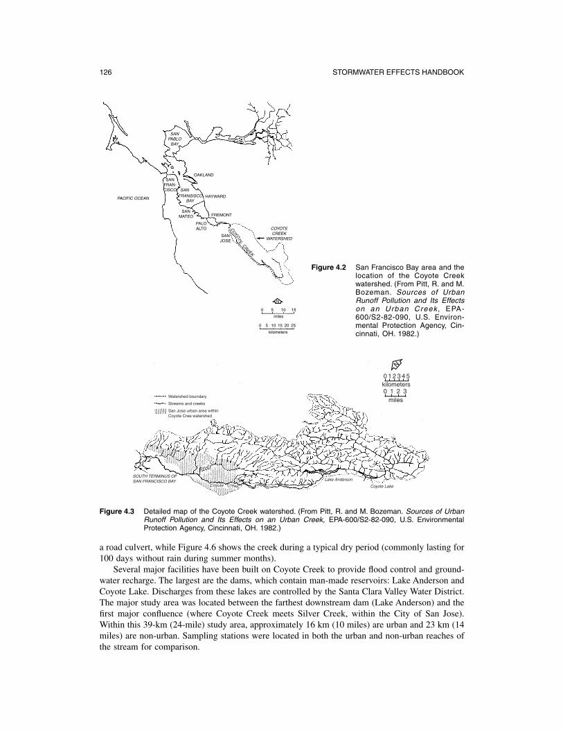
126 STORMWATER EFFECTS HANDBOOK
SAN PABLO
BAY
OAKLAND SAN
FRAN-CISCO
PACIFIC OCEAN
SAN FRANSISCO
BAY HAYWARD
FREMONT SAN
MATEO
PALO ALTO
SAN JOSE
COYOTE CREEK
WATERSHED
CO
YOT
ECRE EK
N
0 5 10 15
0 5 15
20 25
miles
kilometers
1 0
Figure 4.2 San Francisco Bay area and the location of the Coyote Creek watershed. (From Pitt, R. and M. Bozeman. Sources of Urban Runoff Pollution and Its Effects on an Urban Creek , EPA600/S2-82-090, U.S. Environmental Protection Agency, Cincinnati, OH. 1982.)
N
0 1 2 3 4 5 kilometers 0 1 2 3
milesWatershed boundary
Streams and creeks
San Jose urban area within Coyote Cree watershed
SOUTH TERMINUS OF SAN FRANCISCO BAY
Silve rCr
Coyo te Creek
Lake Anderson
Coyote Lake
Figure 4.3 Detailed map of the Coyote Creek watershed. (From Pitt, R. and M. Bozeman. Sources of Urban Runoff Pollution and Its Effects on an Urban Creek, EPA-600/S2-82-090, U.S. Environmental Protection Agency, Cincinnati, OH. 1982.)
a road culvert, while Figure 4.6 shows the creek during a typical dry period (commonly lasting for 100 days without rain during summer months).
Several major facilities have been built on Coyote Creek to provide flood control and groundwater recharge. The largest are the dams, which contain man-made reservoirs: Lake Anderson and Coyote Lake. Discharges from these lakes are controlled by the Santa Clara Valley Water District. The major study area was located between the farthest downstream dam (Lake Anderson) and the first major confluence (where Coyote Creek meets Silver Creek, within the City of San Jose). Within this 39-km (24-mile) study area, approximately 16 km (10 miles) are urban and 23 km (14 miles) are non-urban. Sampling stations were located in both the urban and non-urban reaches of the stream for comparison.
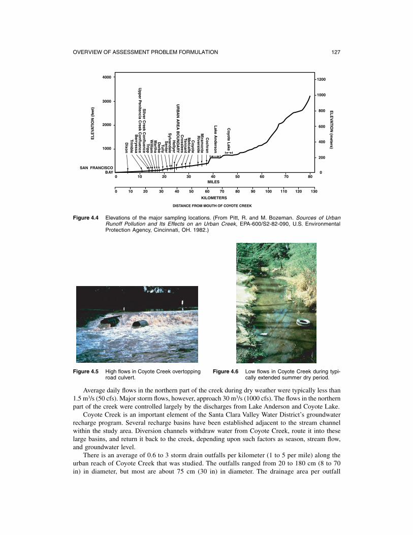
OVERVIEW OF ASSESSMENT PROBLEM FORMULATION 127
4000
Trimb
le B
erryessa U
pp
er Pen
itencia C
reek Co
nflu
ence
Silver C
reek Co
nflu
ence
Tripp
W
illiam
Marth
a D
erbe
Tully
Sen
terS
ylvand
ale H
ellyer
Cro
sslees Ten
nan
t M
etcalfe C
oyote
Riversid
e M
iramo
nte
Co
chran
Lake A
nd
erson
Coyo
te Lake
UR
BA
N A
RE
A B
OU
ND
AR
Y
Dixo
n
1200
1000
3000
800
2000 600
400
1000
200
SAN FRANCISCO BAY 0
0 10 20 30 40 50 60 70 80 MILES
0 10 20 30 40 50 60 70 80 90 100 110 120 130
KILOMETERS
DISTANCE FROM MOUTH OF COYOTE CREEK
Figure 4.4 Elevations of the major sampling locations. (From Pitt, R. and M. Bozeman. Sources of Urban Runoff Pollution and Its Effects on an Urban Creek, EPA-600/S2-82-090, U.S. Environmental Protection Agency, Cincinnati, OH. 1982.)
Figure 4.5 High flows in Coyote Creek overtopping Figure 4.6 Low flows in Coyote Creek during typiroad culvert. cally extended summer dry period.
Average daily flows in the northern part of the creek during dry weather were typically less than 1.5 m3/s (50 cfs). Major storm flows, however, approach 30 m3/s (1000 cfs). The flows in the northern part of the creek were controlled largely by the discharges from Lake Anderson and Coyote Lake.
Coyote Creek is an important element of the Santa Clara Valley Water District’s groundwater recharge program. Several recharge basins have been established adjacent to the stream channel within the study area. Diversion channels withdraw water from Coyote Creek, route it into these large basins, and return it back to the creek, depending upon such factors as season, stream flow, and groundwater level.
There is an average of 0.6 to 3 storm drain outfalls per kilometer (1 to 5 per mile) along the urban reach of Coyote Creek that was studied. The outfalls ranged from 20 to 180 cm (8 to 70 in) in diameter, but most are about 75 cm (30 in) in diameter. The drainage area per outfall
EL
EVA
TIO
N (
feet
) EL
EVA
TIO
N (m
eters)

128 STORMWATER EFFECTS HANDBOOK
Table 4.9 Coyote Creek Drainage Areas above Each Monitoring Station
Sampling Total Area Urban Area Non-urban Area Station (hectares) (hectares) (hectares) Percent Urban
Cochran 49,510 <5 49,510 <0.01 Miramonte 50,260 <5 50,260 <0.01 Metcalfe 52,360 <50 54,360 <0.1 Crosslees 54,030 50 53,980 0.1 Hellyer 54,400 350 54,050 0.6 Sylvandale 54,720 450 54,320 0.7 Senter 55,300 800 50,500 1.5 Derbe 56,300 1740 54,560 3.2 William 56,920 2150 54,770 3.9 Tripp 57,260 2460 54,800 4.5
From Pitt, R. and M. Bozeman. Sources of Urban Runoff Pollution and Its Effects on an Urban Creek, EPA-600/S2-82-090, U.S. Environmental Protection Agency, Cincinnati, OH. 1982.
ranged from 2 to 320 ha (5 to 800 acres), but most of the outfalls drained areas smaller than 40 ha (100 acres).
Table 4.9 describes the drainage areas which cumulatively contribute runoff flows to selected monitoring stations. The urban area stations had about 3 to 5% (1700 to 2500 ha or 4000 to 6000 acres) of their total drainage areas urbanized, whereas the non-urban area stations had less than 0.1% of their drainage areas urbanized. The three stations designated as Hellyer, Sylvandale, and Senter were transition stations (about 0.6 to 1.5% of their drainage areas were urbanized).
Select Monitoring Parameters
The project involved conducting field measurements, observations, sampling, and other studies of Coyote Creek from March 1977 through August 1980. The study focused on the urban reaches of Coyote Creek, extending from Lake Anderson to the confluence with Silver Creek. In this reach of Coyote Creek, there are no known flow or pollutant contributions other than urban runoff. The sampling areas were selected such that each included a stretch of stream several hundred meters long, which met prescribed criteria for physical, biological, and chemical homogeneity.
The following parameters were typically examined at each sampling location:
• Basic hydrologic conditions • Water quality • Sediment properties • General habitat characteristics • Fish • Benthic organisms (e.g., aquatic insects, crustaceans, mollusks) • Attached algae • Rooted aquatic vegetation (e.g., cattails)
Step 4. Project Implementation (Routine Initial Semiquantitative Survey)
Sampling took place during all months during the complete project period. As an example, the biological sampling stressed the spring and summer seasons of all project years, while the water column and sediment samples were conducted approximately monthly.
All water and sediment sampling was conducted manually using either plastic (HDPE) or glass wide-mouth bottles. Sediment core samples were obtained using a liquid carbon dioxide freezing core sampler. All water and sediment samples were comprised of at least six subsamples from the sampling location reach that were composited before analysis. The samples were then appropriately preserved and delivered to a commercial analytical laboratory for EPA-approved analyses.
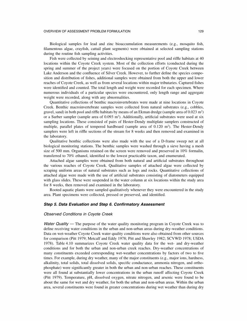
OVERVIEW OF ASSESSMENT PROBLEM FORMULATION 129
Biological samples for lead and zinc bioaccumulation measurements (e.g., mosquito fish, filamentous algae, crayfish, cattail plant segments) were obtained at selected sampling stations during the routine fish sampling activities.
Fish were collected by seining and electroshocking representative pool and riffle habitats at 40 locations within the Coyote Creek system. Most of the collection efforts (conducted during the spring and summer of the project years) were focused on the portion of Coyote Creek between Lake Anderson and the confluence of Silver Creek. However, to further define the species composition and distribution of fishes, additional samples were obtained from both the upper and lower reaches of Coyote Creek, as well as from several locations within major tributaries. Captured fishes were identified and counted. The total length and weight were recorded for each specimen. Where numerous individuals of a particular species were encountered, only length range and aggregate weight were recorded, along with any abnormalities.
Quantitative collections of benthic macroinvertebrates were made at nine locations in Coyote Creek. Benthic macroinvertebrate samples were collected from natural substrates (e.g., cobbles, gravel, sand) in both pool and riffle habitats by means of an Ekman dredge (sample area of 0.023 m2) or a Surber sampler (sample area of 0.093 m2). Additionally, artificial substrates were used at six sampling locations. These consisted of pairs of Hester-Dendy multiplate samplers constructed of multiple, parallel plates of tempered hardboard (sample area of 0.120 m2). The Hester-Dendy samplers were left in riffle sections of the stream for 8 weeks and then removed and examined in the laboratory.
Qualitative benthic collections were also made with the use of a D-frame sweep net at all biological monitoring stations. The benthic samples were washed through a sieve having a mesh size of 500 mm. Organisms retained on the screen were removed and preserved in 10% formalin, transferred to 70% ethanol, identified to the lowest practicable taxon, and enumerated.
Attached algae samples were obtained from both natural and artificial substrates throughout the various reaches of Coyote Creek. Qualitative samples of attached algae were collected by scraping uniform areas of natural substrates such as logs and rocks. Quantitative collections of attached algae were made with the use of artificial substrates consisting of diatometers equipped with glass slides. These were suspended in the water column at six locations within the study area for 8 weeks, then removed and examined in the laboratory.
Rooted aquatic plants were sampled qualitatively whenever they were encountered in the study area. Plant specimens were collected, pressed or preserved, and identified.
Step 5. Data Evaluation and Step 6. Confirmatory Assessment
Observed Conditions in Coyote Creek
Water Quality — The purpose of the water quality monitoring program in Coyote Creek was to define receiving water conditions in the urban and non-urban areas during dry-weather conditions. Data on wet-weather Coyote Creek water quality conditions were also obtained from other sources for comparison (Pitt 1979; Metcalf and Eddy 1978; Pitt and Shawley 1982; SCVWD 1978; USDA 1978). Table 4.10 summarizes Coyote Creek water quality data for the wet- and dry-weather conditions and for both the urban and non-urban creek reaches. Dry-weather concentrations of many constituents exceeded corresponding wet-weather concentrations by factors of two to five times. For example, during dry weather, many of the major constituents (e.g., major ions, hardness, alkalinity, total solids, total dissolved solids, specific conductance, ammonia nitrogen, and orthophosphate) were significantly greater in both the urban and non-urban reaches. These constituents were all found at substantially lower concentrations in the urban runoff affecting Coyote Creek (Pitt 1979). Temperature, pH, dissolved oxygen, nitrate nitrogen, and arsenic were found to be about the same for wet and dry weather, for both the urban and non-urban areas. Within the urban area, several constituents were found in greater concentrations during wet weather than during dry

130 STORMWATER EFFECTS HANDBOOK
Table 4.10 Typical Coyote Water Quality Condition by Location and Season (mg/L unless otherwise noted)
Urban Area Non-Urban Area Wet Dry Wet Dry
Weather Weather Weather Weather
Common Parameters and Major Ions
pH 7 8 8 Temperature 16 17 — 16 Calcium — dissolved 20 100 40 100 Magnesium — dissolved 6 70 20 60 Sodium — dissolved 0.01 — — 20 Potassium — dissolved 2 4 2 2 Bicarbonate 50 150 — 200 Sulfate 20 60 — 40 Chloride 10 60 — 20 Total hardness 70 500 200 600 Total alkalinity 50 300 150 300
Residuals
Total solids 350 1000 600 1000 Total dissolved solids 150 1000 300 1000 Suspended solids 300 4 600 20 Volatile suspended solids 60 2 90 10 Turbidity (NTU) 50 15 — 20
500 — 400Specific conductance (µmhos/cm) 200
Organics and Oxygen Demand Material
Dissolved oxygen (DO) 8 7 — 9 Biochemical oxygen demand (5- 25 — 5 — day) (BOD5)
Chemical oxygen demand (COD) 100 40 90 30 Total organic carbon (TOC) 110 — — 0.6
Nutrients
Total Kjeldahl nitrogen (TKN) 7 0.5 2 <0.3 Nitrate (as N) 0.7 0.8 — 1.2 Nitrite (as N) — 0.02 — <0.002 Ammonia (as N) 0.1 0.8 0.1 0.3 Orthophosphate 0.2 0.5 0.1 0.4
Heavy Metals
Lead (µg/L) 2000 40 200 2 Zinc (µg/L) 400 30 200 20 Copper (µg/L) 20 10 50 5 Chromium (µg/L) 20 10 5 5 Cadmium (µg/L) 5 <1 5 <1 Mercury (µg/L) 1 0.2 1 0.2 Arsenic (µg/L) 4 3 5 2 Iron (µg/L) 10,000 1000 20,000 2000 Nickel (µg/L) 40 <1 80 <1
From Pitt, R. and M. Bozeman. Sources of Urban Runoff Pollution and Its Effects on an Urban Creek, EPA600/S2-82-090, U.S. Environmental Protection Agency, Cincinnati, OH. 1982.
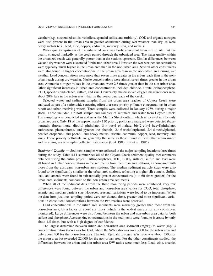
OVERVIEW OF ASSESSMENT PROBLEM FORMULATION 131
weather (e.g., suspended solids, volatile suspended solids, and turbidity). COD and organic nitrogen were also present in the urban area in greater abundance during wet weather than dry, as were heavy metals (e.g., lead, zinc, copper, cadmium, mercury, iron, and nickel).
Water quality upstream of the urbanized area was fairly consistent from site to site, but the quality changed markedly as the creek passed through the urbanized area. The water quality within the urbanized reach was generally poorer than at the stations upstream. Similar differences between wet and dry weather were also noted for the non-urban area. However, the wet-weather concentrations were typically much higher in the urban area than in the non-urban area. Several other constituents were also found in higher concentrations in the urban area than in the non-urban area during wet weather. Lead concentrations were more than seven times greater in the urban reach than in the nonurban reach during dry weather. Nitrite concentrations were almost seven times greater in the urban area. Ammonia nitrogen values in the urban area were 2.8 times greater than in the non-urban area. Other significant increases in urban area concentrations included chloride, nitrate, orthophosphate, COD, specific conductance, sulfate, and zinc. Conversely, the dissolved oxygen measurements were about 20% less in the urban reach than in the non-urban reach of the creek.
Selected water and sediment samples from the urban area reaches of Coyote Creek were analyzed as part of a nationwide screening effort to assess priority pollutant concentrations in urban runoff and urban receiving waters. Three samples were collected in January 1979, during a major storm. These included a runoff sample and samples of sediment and water from Coyote Creek. The sampling was conducted in and near the Martha Street outfall, which is located in a heavily urbanized area. Only 18 of the approximately 120 priority pollutants analyzed were detected (baseneutrals: fluoranthene, diethyl phthalate, di-n-butyl phthalate, bis(2-ethyl hexyl)phthalate, anthracene, phenanthrene, and pyrene; the phenols: 2,4,6-tricholorphenol, 2,4-dimethylphenol, pentachlorophenol, and phenol; and heavy metals: arsenic, cadmium, copper, lead, mercury, and zinc). These priority pollutants are generally the same as those found in most other urban runoff and receiving water samples collected nationwide (EPA 1983, Pitt et al. 1995).
Sediment Quality — Sediment samples were collected at the major sampling locations three times during the study. Table 4.11 summarizes all of the Coyote Creek sediment quality measurements obtained during the entire project. Orthophosphates, TOC, BOD5, sulfates, sulfur, and lead were all found in higher concentrations in the sediments from the urban area stations, as compared with those from the upstream, non-urban area stations. The median sediment particle sizes were also found to be significantly smaller at the urban area stations, reflecting a higher silt content. Sulfur, lead, and arsenic were found in substantially greater concentrations (4 to 60 times greater) for the urban area sediments compared to the non-urban area sediments.
When all of the sediment data from the three monitoring periods were combined, very few differences were found between the urban and non-urban area values for COD, total phosphate, arsenic, and median particle size. However, seasonal variations were found to be important. When the data from just one sampling period were considered alone, greater and more significant variations in constituent concentrations between the two reaches were observed.
Lead concentrations in the urban area sediments were markedly greater than those from the non-urban area, by a factor of about six times (which is the widest margin for any constituent monitored). Large differences were also found between the urban and non-urban area data for both sulfate and phosphate. Average zinc concentrations in the sediments were found to increase by only about 1.5 times, but with a high degree of confidence.
The largest difference between urban and non-urban area sediment (mg/kg) to water (mg/L) concentration ratios (S/W) was for lead, where the S/W ratio was over 3000 for the urban area and only about 400 for the non-urban area. The total Kjeldahl nitrogen S/W ratio was about 5500 for the urban area but exceeded 22,000 for the non-urban area. For the other constituents studied, the differences between the urban and non-urban area S/W ratios were much less. Lead, zinc, arsenic,

132 S
TOR
MW
ATE
R E
FF
EC
TS
HA
ND
BO
OK
From Pitt, R. and M. Bozeman. Sources of Urban Runoff Pollution and Its Effects on an Urban Creek, EPA-600/S2-82-090, U.S. Environmental Protection Agency, Cincinnati,
Confidence that Urban/ Non-Urban
Urban and Non-Urban
Values
<60%
<60%
<60%
85% 85%
80% 65% 96% 97%
Differences
Ratio of Means
1.1
1.1 3.0 0.4
3.2 1.2 6.1 1.5 1.0
COV
0.96 0.78
0.79
0.39 0.81
1.0
1.7
2.4
1.2
St. Dev.
Urban Area Stations above Silver Creek
41,000
4100
1010
3650
10.3
161
132
2.8
37
131,000
14,000
3670
8600
Max
406
400 170
6.6
45 <200
4600
Min
146 1.2
1.5
14
20 30 70
39,300
Mean
2490
4480
13.0
168
430
114
3.6
96
No. of Obs.
13
10
13
13 13 13 13 13
3
COV
0.98
0.54
0.54 0.39 0.94
1.1
1.6
1.7 1.0
Non-Urban Area Stations below Anderson Dam
St. Dev.
34,800
10,500
4085
0.65
11.1 10.2
168
229
25
98,000
29,000
8760
Max
344
478
1.7
28 37 90
<200
7400
<1.0
0.46
Min
138
210
7.5
6.7 14
Coyote Creek Sediment Quality
35,500
Mean
6500
4350
11.1 18.8
148
136
1.2
64
No. of Obs.
7
4 3 7
7 7 7 7 7
Solids, Except for
Chemical oxygen
All Units Are
Particle Size
Orthophosphate Total phosphate
mg/kg Total
Median particle
Total Kjeldahl
Table 4.11
size (µm)
OH. 1982.
demand
nitrogen Sulfate Arsenic Lead Zinc
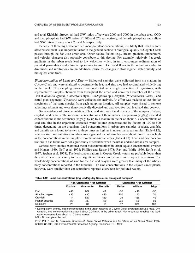
OVERVIEW OF ASSESSMENT PROBLEM FORMULATION 133
and total Kjeldahl nitrogen all had S/W ratios of between 2000 and 5000 in the urban area. COD and total phosphate had S/W ratios of 1300 and 670, respectively, while orthophosphate and sulfate had S/W ratios of only about 20 and 6, respectively.
Because of these high observed sediment pollutant concentrations, it is likely that urban runoff- affected sediment is an important factor in the general decline in biological quality as Coyote Creek passes through the San Jose urban area. Other natural factors (e.g., stream gradient, temperature, and velocity changes) also probably contribute to this decline. For example, relatively flat creek gradients in the urban reach lead to low velocities which, in turn, encourage sedimentation of polluted particulates and allow temperatures to rise. Decreased flows in the urban area (due to diversions and infiltration) are an additional cause for changes in flow regime, water quality, and biological conditions.
Bioaccumulation of Lead and Zinc — Biological samples were collected from six stations in Coyote Creek and were analyzed to determine the lead and zinc they had accumulated while living in the creek. This sampling program was restricted to a single collection of organisms, with representative samples obtained from throughout the urban and non-urban stretches of the creek. Fish (Gambusia affinis), filamentous algae (Cladophora sp.), crayfish (Procambarus clarkii), and cattail plant segments (Typha sp.) were collected for analysis. An effort was made to collect similar specimens of the same species from each sampling location. All samples were rinsed to remove adhering sediment and were then chemically digested and analyzed for total lead and zinc content.
Some evidence of bioaccumulation of lead and zinc was found in many of the samples of algae, crayfish, and cattails. The measured concentrations of these metals in organisms (mg/kg) exceeded concentrations in the sediments (mg/kg) by up to a maximum factor of about 6. Concentrations of lead and zinc in the organisms exceeded water column concentrations by factors of 100 to 500 times, depending on the organism. Lead concentrations in urban area samples of algae, crayfish, and cattails were found to be two to three times as high as in non-urban area samples (Table 4.12), whereas zinc concentrations in urban area algae and cattail samples were about three times as high as the concentrations in the samples from the non-urban areas (Table 4.13). Lead and zinc concen- trations in fish tissue were not significantly different between the urban and non-urban area samples.
Several early studies examined metal bioaccumulations in urban aquatic environments (Wilber and Hunter 1980; Neff et al. 1978; Phillips and Russo 1978; Ray and While 1976; Rolfe et al. 1977; Spehan et al. 1978). The lead concentrations in Coyote Creek waters are probably lower than the critical levels necessary to cause significant bioaccumulation in most aquatic organisms. The whole-body concentrations of zinc for the fish and crayfish were greater than many of the whole- body concentrations reported in the literature. The zinc concentrations in the Coyote Creek plants, however, were smaller than concentrations reported elsewhere for polluted waters.
Table 4.12 Lead Concentrations (mg lead/kg dry tissue) in Biological Samplesa
Non-Urbanized Area Stations Urbanized Area Stations Cochran Miramonte Metcalfe Derbe William Tripp
Fish <40 NS NS <30 <40 <50 Attached algae <20 <30 <30 200 170 70 Crayfish 14 NS <30 29 <36 40 Higher aquatics <20 <30 <30 <30 <50 60 Sediment 28 37 16 37 370 400
a During storm events, lead concentrations in the urban reaches of Coyote Creek averaged about 2 mg/L. Dry weather, lead concentrations averaged about 0.04 mg/L in the urban reach. Non-urbanized reaches had lead water concentrations about 1/10 these values.
NS = No sample collected.
From Pitt, R. and M. Bozeman. Sources of Urban Runoff Pollution and Its Effects on an Urban Creek, EPA600/S2-82-090, U.S. Environmental Protection Agency, Cincinnati, OH. 1982.

134 STORMWATER EFFECTS HANDBOOK
Table 4.13 Zinc Concentrations (mg zinc/kg dry tissue) in Biological Samplesa
Non-Urbanized Area Stations Cochran Miramonte Metcalfe Derbe William Tripp
Urbanized Area Stations
Fish 135 NS NS 100 120 130 Attached algae 6.5 24 17 160 135 69 Crayfish 80 NS 90 89 140 62 Higher aquatics 9 78 26 40 150 210 Sediment 70 70 14 30 120 70
a During storm events, zinc concentration in the urban reaches of Coyote Creek averaged about 0.4 mg/L. Dry-weather zinc concentration in the urban reaches averaged about 0.03 mg/L. Non-urban reach water sample zinc concentrations were about half of these values.
NS = No sample collected.
From Pitt, R. and M. Bozeman. Sources of Urban Runoff Pollution and Its Effects on an Urban Creek, EPA-600/S2-82-090, U.S. Environmental Protection Agency, Cincinnati, OH. 1982.
Aquatic Biota Conditions
Fish — The fish fauna known to exist in the Coyote Creek drainage system at the time of the study was comprised of 27 species, 11 of which are native California fishes. The remainder were introduced through stocking by the California Department of Fish and Game and by the activities of bait dealers, fisherman, farm pond owners, and others. Although a relatively large variety of fish species was present in the Coyote Creek drainage, the existing distribution of some species was not widespread. Both Lake Anderson and Coyote Lake reservoirs sustained warm-water sport fisheries, and several of the fish species reported from the drainage were apparently confined to the specific habitat provided by those reservoirs. This included brown bullhead, channel catfish, Mississippi silverside, pumpkinseed, and redear sunfish. Of the remaining 22 species of fish known in Coyote Creek, 21 were encountered during this study, in which a total of 7198 fish were collected from 40 locations throughout the drainage. Rainbow trout and riffle sculpin were captured only in the headwater reaches and tributary streams of Coyote Creek. Likewise, Sacramento squawfish were found only in the upper reaches of the creek and reportedly have not been encountered downstream of Lake Anderson since 1960 (Scoppettone and Smith 1978). Seventeen fish species were collected from the major study area between Lake Anderson and the confluence of Silver Creek. Speckled dace, a native species previously reported to occur in the study area, was not encountered. Pacific lamprey, an anadromous species which moves into fresh water to spawn, was found only in and around the mouth of Upper Penitencia Creek, a tributary that enters the lower reaches of Coyote Creek.
Introduced fishes often cause radical changes in the nature of the fish fauna present in a given water body or drainage system. In many cases, they become the dominant fishes because they are able to outcompete the native fish for food or space, or they may possess greater tolerance to environmental stress. In general, introduced species are most abundant in aquatic habitats modified by man, while native fish tend to persist mostly in undisturbed areas (Moyle and Nichols 1973). Such was apparently the case within Coyote Creek. As seen in Table 4.14, samples from the non- urban portion of the study area were dominated by an assemblage of native fish species such as hitch, threespine stickleback, Sacramento sucker, and prickly sculpin. Collectively, native species comprised 89% of the number and 79% of the biomass of the 2379 fish collected from the upper reaches of the study area. In contrast, native species accounted for only 7% of the number and 31% of the biomass of the 2899 fish collected from the urban reach of the study area.
Hitch was the most numerous native fish species present. Hitch generally exhibit a preference for quiet water habitat and are characteristic of warm, low elevation lakes, sloughs, sluggish rivers, and ponds (Calhoun 1966; Moyle and Nichols 1976). In streams of the San Joaquin River system in the Sierra Nevada foothills of central California, Moyle and Nichols (1973) found hitch to be
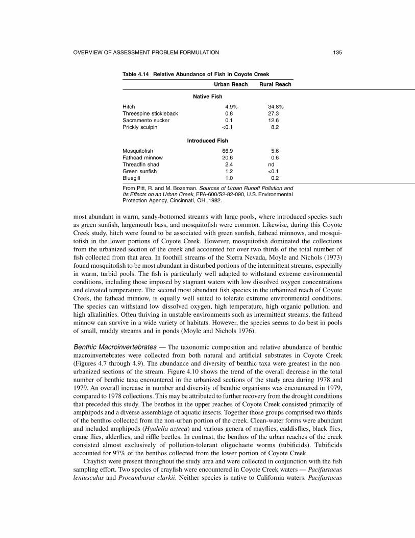
OVERVIEW OF ASSESSMENT PROBLEM FORMULATION 135
Table 4.14 Relative Abundance of Fish in Coyote Creek
Urban Reach Rural Reach
Native Fish
Hitch 4.9% 34.8% Threespine stickleback 0.8 27.3 Sacramento sucker 0.1 12.6 Prickly sculpin <0.1 8.2
Introduced Fish
Mosquitofish 66.9 5.6 Fathead minnow 20.6 0.6 Threadfin shad 2.4 nd Green sunfish 1.2 <0.1 Bluegill 1.0 0.2
From Pitt, R. and M. Bozeman. Sources of Urban Runoff Pollution and Its Effects on an Urban Creek, EPA-600/S2-82-090, U.S. Environmental Protection Agency, Cincinnati, OH. 1982.
most abundant in warm, sandy-bottomed streams with large pools, where introduced species such as green sunfish, largemouth bass, and mosquitofish were common. Likewise, during this Coyote Creek study, hitch were found to be associated with green sunfish, fathead minnows, and mosqui- tofish in the lower portions of Coyote Creek. However, mosquitofish dominated the collections from the urbanized section of the creek and accounted for over two thirds of the total number of fish collected from that area. In foothill streams of the Sierra Nevada, Moyle and Nichols (1973) found mosquitofish to be most abundant in disturbed portions of the intermittent streams, especially in warm, turbid pools. The fish is particularly well adapted to withstand extreme environmental conditions, including those imposed by stagnant waters with low dissolved oxygen concentrations and elevated temperature. The second most abundant fish species in the urbanized reach of Coyote Creek, the fathead minnow, is equally well suited to tolerate extreme environmental conditions. The species can withstand low dissolved oxygen, high temperature, high organic pollution, and high alkalinities. Often thriving in unstable environments such as intermittent streams, the fathead minnow can survive in a wide variety of habitats. However, the species seems to do best in pools of small, muddy streams and in ponds (Moyle and Nichols 1976).
Benthic Macroinvertebrates — The taxonomic composition and relative abundance of benthic macroinvertebrates were collected from both natural and artificial substrates in Coyote Creek (Figures 4.7 through 4.9). The abundance and diversity of benthic taxa were greatest in the non- urbanized sections of the stream. Figure 4.10 shows the trend of the overall decrease in the total number of benthic taxa encountered in the urbanized sections of the study area during 1978 and 1979. An overall increase in number and diversity of benthic organisms was encountered in 1979, compared to 1978 collections. This may be attributed to further recovery from the drought conditions that preceded this study. The benthos in the upper reaches of Coyote Creek consisted primarily of amphipods and a diverse assemblage of aquatic insects. Together those groups comprised two thirds of the benthos collected from the non-urban portion of the creek. Clean-water forms were abundant and included amphipods (Hyalella azteca) and various genera of mayflies, caddisflies, black flies, crane flies, alderflies, and riffle beetles. In contrast, the benthos of the urban reaches of the creek consisted almost exclusively of pollution-tolerant oligochaete worms (tubificids). Tubificids accounted for 97% of the benthos collected from the lower portion of Coyote Creek.
Crayfish were present throughout the study area and were collected in conjunction with the fish sampling effort. Two species of crayfish were encountered in Coyote Creek waters — Pacifastacus leniusculus and Procambarus clarkii. Neither species is native to California waters. Pacifastacus

136 STORMWATER EFFECTS HANDBOOK
Figure 4.7 Natural substrate sampling using a Figure 4.8 Removing benthic macroinvertebrate Surber sampler in Coyote Creek. samples from Surber sampler.
leniusculus was collected in the non-urbanized section of the study area. It is typically found in a wide variety of habitats including large rivers, swift or sluggish streams, lakes, and, occasion- ally, muddy sloughs. Procambarus clarkii was collected in both the urbanized and non-urban- ized sections of the stream. The species prefers sloughs where the water is relatively warm and vegetation plentiful; however, it is also found in
Figure 4.9 Artificial substrate sampling using a large streams. Because of its burrowing activities Hester-Dendy multiplate sampler in P. clarkii often becomes a nuisance by damagingCoyote Creek. irrigation ditches and earthen dams.
Attached Algae — Qualitative samples from natural substrates indicated that the filamentous alga Cladophora sp. was found throughout the study area. However, its growth reached greatest pro- portions in the upper sections of the stream. Table 4.15 presents the taxonomic composition and relative abundance of diatoms collected from artificial substrates (Figure 4.11) placed at selected sample locations. The periphyton of the non-urban reaches of the stream was dominated by the genera Cocconeis and Achnanthes. The genera Nitzschia and Navicula, generally accepted to be more pollution-tolerant forms, dominated the periphyton of the urbanized reaches of Coyote Creek.
Rooted Aquatic Vegetation — Rooted aquatic plants were not greatly abundant in the Coyote Creek study area. Submerged macrophytes were restricted entirely to the upper reaches of the study area and consisted of occasional stands of sago pondweed (Potamogeton pectinatus) and curly-leaf pondweed (P. crispus). Emergent forms consisted of water primrose (Jussiaea sp.), confined to several areas in the non-urban reach of the stream, and numerous small stands of cattails (Typha sp.) sparsely distributed throughout the length of the study area.
Step 7. Project Conclusions
The biological investigations in Coyote Creek indicated distinct differences in the taxonomic composition and relative abundance of the aquatic biota present in Coyote Creek. The non-urban
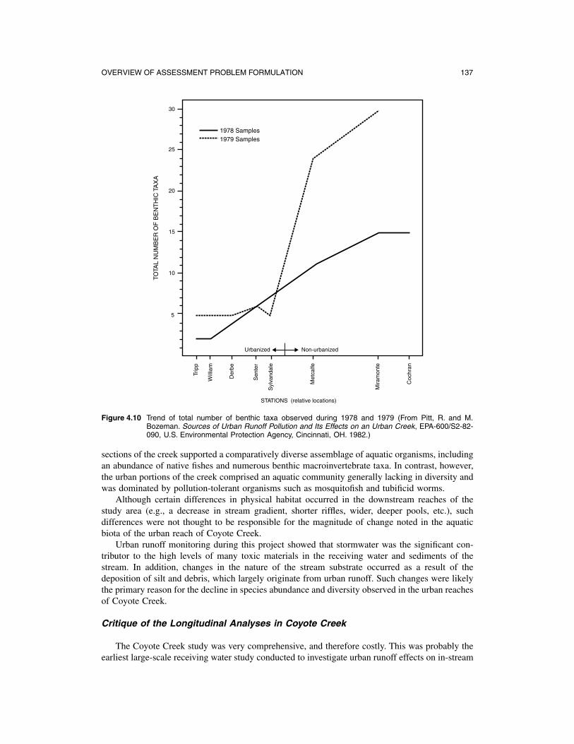
OVERVIEW OF ASSESSMENT PROBLEM FORMULATION 137
30
1978 Samples 1979 Samples
Urbanized Non-urbanized
25
20
15
10
5
STATIONS (relative locations)
Figure 4.10 Trend of total number of benthic taxa observed during 1978 and 1979 (From Pitt, R. and M. Bozeman. Sources of Urban Runoff Pollution and Its Effects on an Urban Creek, EPA-600/S2-82090, U.S. Environmental Protection Agency, Cincinnati, OH. 1982.)
sections of the creek supported a comparatively diverse assemblage of aquatic organisms, including an abundance of native fishes and numerous benthic macroinvertebrate taxa. In contrast, however, the urban portions of the creek comprised an aquatic community generally lacking in diversity and was dominated by pollution-tolerant organisms such as mosquitofish and tubificid worms.
Although certain differences in physical habitat occurred in the downstream reaches of the study area (e.g., a decrease in stream gradient, shorter riffles, wider, deeper pools, etc.), such differences were not thought to be responsible for the magnitude of change noted in the aquatic biota of the urban reach of Coyote Creek.
Urban runoff monitoring during this project showed that stormwater was the significant con- tributor to the high levels of many toxic materials in the receiving water and sediments of the stream. In addition, changes in the nature of the stream substrate occurred as a result of the deposition of silt and debris, which largely originate from urban runoff. Such changes were likely the primary reason for the decline in species abundance and diversity observed in the urban reaches of Coyote Creek.
Critique of the Longitudinal Analyses in Coyote Creek
The Coyote Creek study was very comprehensive, and therefore costly. This was probably the earliest large-scale receiving water study conducted to investigate urban runoff effects on in-stream
TOTA
L N
UM
BE
R O
F B
EN
TH
IC T
AX
A
Trip
p
Will
iam
Der
be
Sen
ter
Syl
vand
ale
Met
calfe
Mira
mon
te
Coc
hran

138 STORMWATER EFFECTS HANDBOOK
Table 4.15 Taxonomic Composition and Relative Abundance of Diatoms Collected on Glass Slides in Coyote Creek during the Spring of 1978
Relative Abundance (%) of each Taxon within the Sample Non-Urban Area Stations Urban Area Stations
Taxon Cochran Miramonte Metcalfe Derbe Williams Tripp
Centrales Coscinodiscaceae
Melosira sp. 0.4 — — — 1.2 0.8 Pennales
Diatomaceae Diatoma vulgare 0.4 — 1.5 — — —
Fragilariaceae — — — 0.8 0.9 0.4 Synedra sp.
Achnanthaceae Achanthes lanceolata 20.6 37.8 56.1 49.8 0.9 1.6 Rhoicosphenia curvata 0.4 — — 1.2 — — Cocconeis pediculus 15.0 18.2 0.4 — — — Cocconeis placentula 62.4 44.0 41.2 — — —
Naviculaceae Navicula spp. — — — — 10.5 23.8 Diploneis sp. — — — — 2.4 — Frustulia rhomboides — — — — 0.4 — Gyrosigma sp. — — — — — 0.4
Gomphonenataceae Gomphonema sp. — — — 2.8 6.9 0.8
Cybellaceae Cymbella sp. 0.8 — — — 2.0 0.4 Rhopalodia spp. — — — — — 0.4
Nitzschiaceae Nitzachia sp. — — 0.8 43.4 67.5 70.6 Denticula elegans — — — — 2.4 0.4
Surirellaceae Cymatopleura solea — — — — 0.9 — Surirella sp. — — — 2.0 4.0 0.4
Total Number Frustules/mm2 5545 4950 1874 4488 1189 4575
From Pitt, R. and M. Bozeman. Sources of Urban Runoff Pollution and Its Effects on an Urban Creek, EPA-600/S282-090, U.S. Environmental Protection Agency, Cincinnati, OH. 1982.
biological conditions. As such, many elements were considered in the site investigation. The project included field sampling over a period of 3 years, and more than 40 sampling sites were periodically visited. A broad list of biological, chemical, and physical measurements was obtained. Even though the project was compre- hensive, several omissions seem obvious. The most notable is the lack of toxicity testing. Some
Figure 4.11 Artificial substrate diatometer sampler limited laboratory fathead minnow 96-hour expo-
being loaded with glass microscope sure tests were conducted as part of the study, slides in Coyote Creek. but were inconclusive and therefore not reported.
The project was also conducted before effective and less costly in situ toxicity tests were developed. Another element that was missing was comprehensive habitat surveys. Formalized habitat survey procedures detailed in this book (Chapter 6 and Appendix A) would have been very useful during the Coyote Creek study. Finally, because the study design did not have any precedence, it was probably inefficient in that it obtained more information than was actually needed, and at more locations than necessary.

OVERVIEW OF ASSESSMENT PROBLEM FORMULATION 139
The longitudinal study design is very helpful in that gradients of conditions can be examined. The Coyote Creek study examined a very large number of locations along the creek in an attempt to identify locations that were partially degraded, but still in acceptable condition. When these locations are identified, watershed modeling can be used to calculate the assimilative capacity of the stream, which can then be used to determine necessary stormwater controls to provide these conditions farther downstream. Unfortunately, Coyote Creek was found to degrade very rapidly at the edge of development. Additional monitoring locations were therefore added in an attempt to isolate the degradation gradient. The highly variable conditions in the creek at the edge of urban- ization were likely due to major flow changes seasonally and from year-to-year, preventing iden- tification of an acceptably degraded site.
In many cases, a longitudinal study design can be combined with the other two major types of designs (parallel and trend studies) to obtain additional information. The trend case study presented is for a trend with time, but a trend with distance can also be evaluated using similar statistical procedures described in Chapter 7.
Example of Parallel Creeks Experimental Design — Kelsey and Bear Creeks, Bellevue, WA, Receiving Water Study
Several separate urban stormwater projects (as part of the U.S. EPA’s Nationwide Urban Runoff Program, or NURP) were conducted in Bellevue, WA, to address the three major phases in designing an urban runoff control program (quantifying the specific local urban runoff receiving water problems, determining the sources of the problem pollutants, and selecting the most appropriate control measures). These projects were conducted from 1977 through 1982 and constitute one of the most comprehensive urban runoff/receiving water impact research programs ever conducted.
The U.S. Geological Survey (USGS) through its Tacoma, WA, office, conducted one of the projects, which was funded by the USGS and the Water Planning Division of EPA. The USGS (Ebbert et al. 1983; Prych and Ebbert undated) intensively monitored urban runoff quality and quantity from three residential areas in Bellevue and evaluated the effectiveness of a detention facility. Wet and dry atmospheric sources were also monitored by the USGS.
The University of Washington’s Civil Engineering Department and the College of Fisheries Research Institute prepared five reports based on their studies, which were funded by the Corvallis Environmental Research Laboratory of EPA (Pedersen 1981; Perkins 1982; Richey et al. 1981; Richey 1982; Scott et al. 1982). Generally, the University of Washington’s projects evaluated the receiving water conditions for direct impairments of beneficial uses.
The Municipality of Metropolitan Seattle (METRO) research was funded by Region X of EPA and was prepared by Galvin and Moore (1982). METRO analyzed many source area, urban runoff, and creek samples for metallic and organic priority pollutants.
The City of Bellevue also conducted a study, which was funded by the Storm and Combined Sewer Section of EPA and the City of Bellevue. The Bellevue report was prepared by Pitt (1985) and Pitt and Bissonnette (1984). The City of Bellevue collected and analyzed urban runoff and baseflow samples using flow-weighted techniques for more than 300 storms from two residential areas, in addition to extensively evaluating street and sewerage cleaning as stormwater manage- ment practices.
Bellevue’s moderate climate has a mean annual precipitation of about 1.1 m ( 44 in) which occurs mostly as rainfall from October through May. Most of the rainfall results from frontal storms formed over the Pacific Ocean. During fall and winter months, low to moderate rainfall intensities are common. Even though the runoff quality was found to be much cleaner than in other locations in the United States, the urban creek was significantly degraded when compared to the rural creek, but still supported a productive, but limited and unhealthy salmonid fishery. Many of the fish in the urban creek, however, had respiratory anomalies. The urban creek was not grossly polluted, but flooding from urban developments has increased dramatically in recent years. These increased
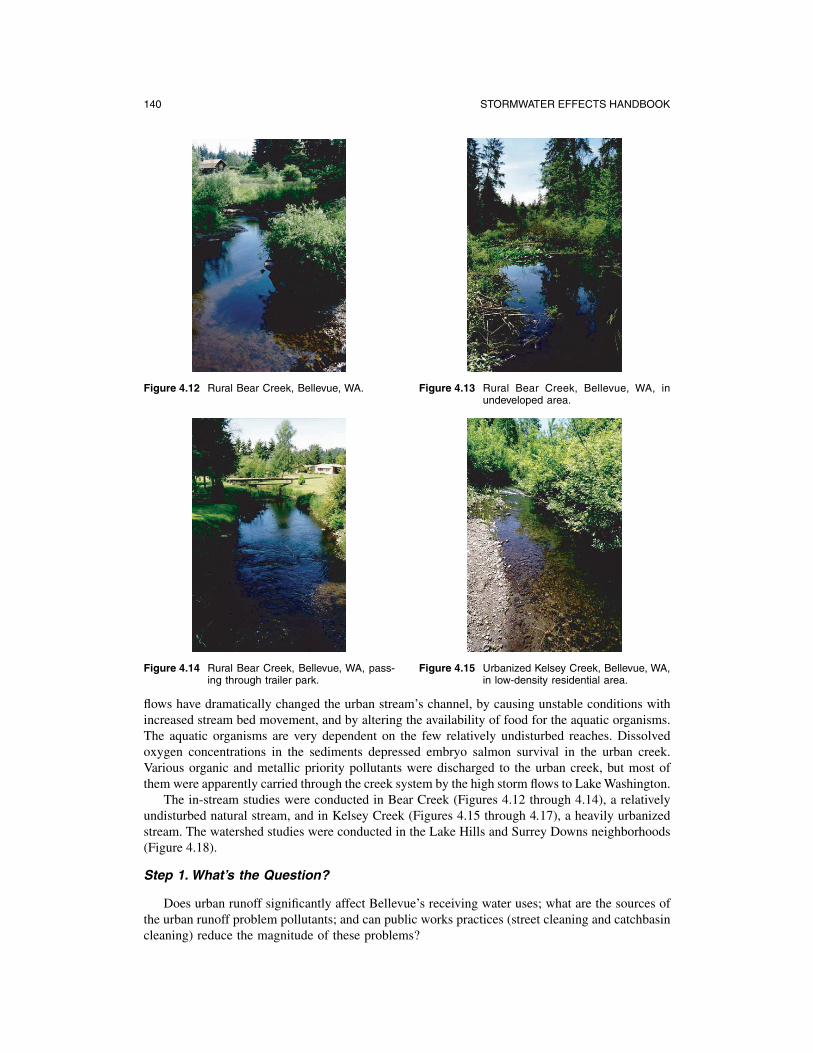
140 STORMWATER EFFECTS HANDBOOK
Figure 4.12 Rural Bear Creek, Bellevue, WA. Figure 4.13 Rural Bear Creek, Bellevue, WA, in undeveloped area.
Figure 4.14 Rural Bear Creek, Bellevue, WA, pass- Figure 4.15 Urbanized Kelsey Creek, Bellevue, WA, ing through trailer park. in low-density residential area.
flows have dramatically changed the urban stream’s channel, by causing unstable conditions with increased stream bed movement, and by altering the availability of food for the aquatic organisms. The aquatic organisms are very dependent on the few relatively undisturbed reaches. Dissolved oxygen concentrations in the sediments depressed embryo salmon survival in the urban creek. Various organic and metallic priority pollutants were discharged to the urban creek, but most of them were apparently carried through the creek system by the high storm flows to Lake Washington.
The in-stream studies were conducted in Bear Creek (Figures 4.12 through 4.14), a relatively undisturbed natural stream, and in Kelsey Creek (Figures 4.15 through 4.17), a heavily urbanized stream. The watershed studies were conducted in the Lake Hills and Surrey Downs neighborhoods (Figure 4.18).
Step 1. What’s the Question?
Does urban runoff significantly affect Bellevue’s receiving water uses; what are the sources of the urban runoff problem pollutants; and can public works practices (street cleaning and catchbasin cleaning) reduce the magnitude of these problems?
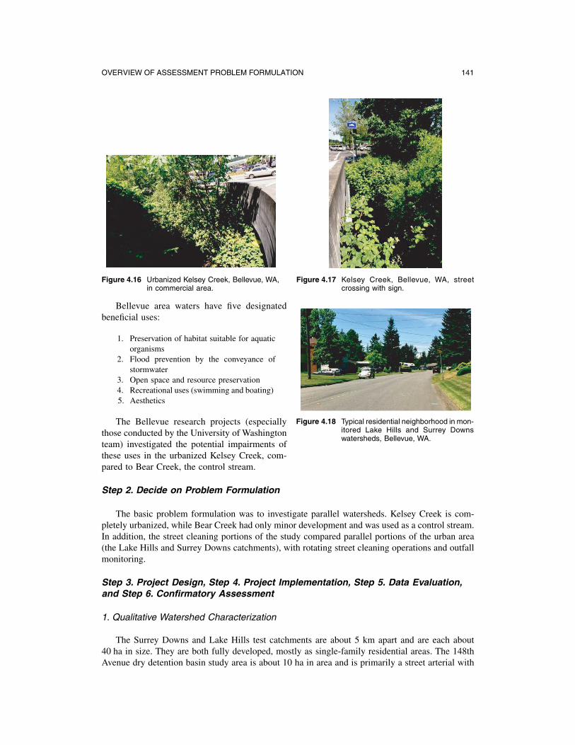
OVERVIEW OF ASSESSMENT PROBLEM FORMULATION 141
Figure 4.16 Urbanized Kelsey Creek, Bellevue, WA, Figure 4.17 Kelsey Creek, Bellevue, WA, street in commercial area. crossing with sign.
Bellevue area waters have five designated beneficial uses:
1. Preservation of habitat suitable for aquatic organisms
2. Flood prevention by the conveyance of stormwater
3. Open space and resource preservation 4. Recreational uses (swimming and boating) 5. Aesthetics
The Bellevue research projects (especially those conducted by the University of Washington itored Lake Hills and Surrey Downs
watersheds, Bellevue, WA.
Figure 4.18 Typical residential neighborhood in mon
team) investigated the potential impairments of these uses in the urbanized Kelsey Creek, com- pared to Bear Creek, the control stream.
Step 2. Decide on Problem Formulation
The basic problem formulation was to investigate parallel watersheds. Kelsey Creek is com- pletely urbanized, while Bear Creek had only minor development and was used as a control stream. In addition, the street cleaning portions of the study compared parallel portions of the urban area (the Lake Hills and Surrey Downs catchments), with rotating street cleaning operations and outfall monitoring.
Step 3. Project Design, Step 4. Project Implementation, Step 5. Data Evaluation, and Step 6. Confirmatory Assessment
1. Qualitative Watershed Characterization
The Surrey Downs and Lake Hills test catchments are about 5 km apart and are each about 40 ha in size. They are both fully developed, mostly as single-family residential areas. The 148th Avenue dry detention basin study area is about 10 ha in area and is primarily a street arterial with

142 STORMWATER EFFECTS HANDBOOK
adjacent landscaping. The Surrey Downs area was developed in the late 1950s. Most of the slopes in the basin are moderate with some steeper slopes on the west side of the area. About 60% of the Surrey Downs area is pervious. Back and front yards make up most of the land surface area, while the streets make up 10%. There is relatively little automobile traffic in the Surrey Downs area and the on-street parking density is low. The storm drainage system discharges into an artificial pond located in an adjacent development. This pond discharges into Mercer Slough, which eventually drains to Lake Washington and Puget Sound. The Surrey Downs catchment ranges in elevation from about 3 to 55 m.
The Lake Hills catchment is about 41 ha in size and contains the St. Louise parish church and school in addition to single-family homes. These homes were also developed in the 1950s. Lake Hills has a slightly larger percentage of pervious area than Surrey Downs, but a slightly smaller typical lot size. The slopes in Lake Hills are also more moderate (with a few exceptions) than those found in Surrey Downs. Most of the streets in Lake Hills also carry low volumes of traffic and have low parking densities, except for two busy roads which cross through the area. The Lake Hills storm drainage system discharges into a short open channel which joins Kelsey Creek just downstream from Larsen Lake. Kelsey Creek also discharges into Mercer Slough and finally into Lake Wash- ington and Puget Sound. The elevation of the Lake Hills study catchment ranges from 80 to 125 m.
The 148th Avenue S.E. catchment was used to investigate the effects of a dry detention facility on stormwater quality. The drainage area is about 10 ha. Slightly more than one fourth of this area is the actual street surface of 148th Avenue S.E., a divided, four-lane arterial. Other impervious areas include sidewalks, parking lots, office buildings, and parts of Robins Wood Elementary School.
The soils in all three of these test catchments are mostly the Arents-Alderwood variety, having 6 to 15% slopes. The surface soils are made up of gravelly sand loams with an estimated natural permeability of between 50 and 150 mm/hour. The total water capacity of this soil horizon is about 20 mm.
A demographic survey was conducted in the test catchments by the City of Bellevue at the beginning of the project (in 1977). Slightly more than three people per household were reported in both basins, while the population density per hectare was about 30 in Lake Hills and about 23 in Surrey Downs. More than half of the people in both basins had no dogs or cats, with the remainder of the households having one or more of each. Slightly more than two cars per household were reported, with about 10% of the households in each basin reporting four or more cars. Most of the automobile oil was disposed of properly in the household garbage or recycled, but between 5 and 10% of the households used oil to treat fence posts, dumped it onto the ground, or into the storm sewers. Most of the people carried their grass and leaves to the dump, or put them into the garbage, and about one third composted the organic debris on their lots.
2. Stream Characterization
Kelsey Creek flows through the City of Bellevue, while Bear Creek is about 30 km farther east. Kelsey Creek drains a watershed about 3200 ha in area, which is predominantly urban. About 54% of the Kelsey Creek watershed has single- and multiple-family residences, 24% has commercial or light industrial uses, and 22% has parks and undeveloped areas. A main channel of Kelsey Creek starts at Larson Lake and flows about 12 km through the City of Bellevue before discharging into Lake Washington. The USGS has continuously monitored Kelsey Creek flows since 1959 at a location about 2.5 km upstream from Lake Washington. Kelsey Creek is a relatively narrow stream with a mild slope. The mean channel slope is about 1.5% and the bank full width ranges from about 3.5 to 6.5 m in the study area. Along much of its length, Kelsey Creek appears disturbed. Channelization, riprapping, storm drain outfalls, scoured and eroded banks, and culverts are com- mon. The stream bank (riparian) vegetation is mostly composed of low growing alder and vine maple with scattered big leaf maples and western red cedar trees. The understory is dominated by blackberry bushes.
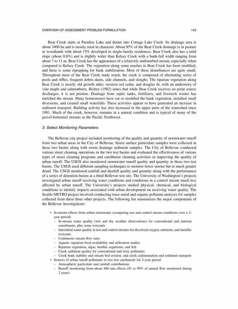
OVERVIEW OF ASSESSMENT PROBLEM FORMULATION 143
Bear Creek starts at Paradise Lake and drains into Cottage Lake Creek. Its drainage area is about 3400 ha and is mostly rural in character. About 85% of the Bear Creek drainage is in pasture or woodlands with about 15% developed in single-family residences. Bear Creek also has a mild slope (about 0.6%) and is slightly wider than Kelsey Creek with a bank-full width ranging from about 7 to 11 m. Bear Creek has the appearance of a relatively undisturbed stream, especially when compared to Kelsey Creek. The vegetation along some reaches in Bear Creek has been modified, and there is some riprapping for bank stabilization. Most of these disturbances are quite small. Throughout most of the Bear Creek study reach, the creek is composed of alternating series of pools and riffles, frequent debris dams, side channels, and sloughs. The riparian vegetation along Bear Creek is mostly old growth alder, western red cedar, and douglas fir, with an understory of vine maple and salmonberry. Richey (1982) states that while Bear Creek receives no point source discharges, it is not pristine. Drainage from septic tanks, fertilizers, and livestock wastes has enriched the stream. Many homeowners have cut or modified the bank vegetation, installed small diversions, and created small waterfalls. These activities appear to have generated an increase in sediment transport. Building activity has also increased in the upper parts of the watershed since 1981. Much of the creek, however, remains in a natural condition and is typical of many of the gravel-bottomed streams in the Pacific Northwest.
3. Select Monitoring Parameters
The Bellevue city project included monitoring of the quality and quantity of stormwater runoff from two urban areas in the City of Bellevue. Street surface particulate samples were collected in these two basins along with storm drainage sediment samples. The City of Bellevue conducted various street cleaning operations in the two test basins and evaluated the effectiveness of various types of street cleaning programs and catchbasin cleaning activities in improving the quality of urban runoff. The USGS also monitored stormwater runoff quality and quantity in these two test basins. The USGS used different sampling techniques to monitor fewer storms but in much greater detail. The USGS monitored rainfall and dustfall quality and quantity along with the performance of a series of detention basins at a third Bellevue test site. The University of Washington’s projects investigated urban runoff receiving water conditions and conditions in a control stream much less affected by urban runoff. The University’s projects studied physical, chemical, and biological conditions to identify impacts associated with urban development on receiving water quality. The Seattle METRO project involved conducting trace metal and organic pollutant analyses for samples collected from these three other projects. The following list summarizes the major components of the Bellevue investigations:
• In-stream effects from urban stormwater (comparing test and control stream conditions over a 2- year period) – In-stream water quality (wet and dry weather observations) for conventional and nutrient
constituents, plus some toxicants – Interstitial water quality in test and control streams for dissolved oxygen, nutrients, and metallic
toxicants – Continuous stream flow rates – Aquatic organism food availability and utilization studies – Riparian vegetation, algae, benthic organisms, and fish – Creek sediment quality for conventional and toxic pollutants – Creek bank stability and stream bed erosion, and creek sedimentation and sediment transport
• Sources of urban runoff pollutants in two test catchments for 2-year period – Atmospheric particulate and rainfall contributions – Runoff monitoring from about 400 rain effects (91 to 99% of annual flow monitored during
2 years)

144 STORMWATER EFFECTS HANDBOOK
– Stormwater quality from more than 200 events for conventional, nutrient, and toxic constituents (200 to 1000 analyses per constituent)
– Baseflow quality from about 25 sampling periods for conventional, nutrient, and toxic constituents
– Street dirt characteristics from about 600 samples (loading, particle size, washoff, and chemical quality)
– Sewerage and catchbasin sediment accumulations over 2-year period (accumulation and quality) from about 200 inlets
• Effectiveness of urban runoff controls – Monitored street dirt loadings and runoff characteristics at two test catchments over 2-year
period, comparing none with three times a week street cleaning effort – Measured changes in catchbasin sump accumulations of pollutants in about 200 inlets over 2
years in two catchments – Monitored influent and effluent from a dry detention pond for the 20 storms during the 2-year
period when flows were sufficient to enter the pond system
Observations
Effects of Urban Runoff on Bellevue’s Stream’s Beneficial Uses — Richey (1982) summa- rizes some of the beneficial use impairments that the University of Washington study team addressed. Urbanization and stormwater runoff discharges to streams can have a wide variety of effects on these receiving waters. These include increased runoff, decreased surface storage, decreased transpiration, decreased infiltration, and a degradation in water quality. These effects may be either long term or intermittent. Changes in channel geomorphology caused by channel- ization in the clearing of stream bank vegetation may cause permanent stresses to the stream. Changes in the stream flows during runoff events, such as rapidly rising and falling hydrographs and increased total flows and peak discharges, are intermittent stress factors. The discharge and transport of pollutants can act as an intermittent stress factor, but the storage of these pollutants in the stream system (in the sediments or bioaccumulation) can act as a long-term or chronic stress factor. Therefore, it is necessary to identify not only the causative factor in impairing receiving water quality but also the times when these effects occur. Elevated concentrations of toxic materials in the runoff may affect receiving water organisms during a runoff event. However, they may also accumulate in the sediments and not affect the receiving water aquatic life until some time after they were discharged.
Richey points out the difficulty in identifying problem pollutants or their causes based upon their different destructive powers. She presents a hypothetical example where the gradual introduc- tion of toxic pollutants in the receiving water results in a decline of fish species diversity and system productivity. Because the watershed has been urbanizing, increased flows have also occurred. If it is assumed that the increased flows causing flooding and scouring in the water body were the most important element restricting the fish populations, an abatement program incorporating detention facilities to reduce these flooding problems may be implemented. However, the input of toxic substances may not be reduced and significant improvements in the beneficial use may not occur. She concludes that it is very important to study all effects on a receiving body including hydrology, geomorphology, and pollutant inputs.
Scott et al. (1982) state that factors contributing to the instability of the physical receiving water system are relatively easy to identify but that their combined effect on the receiving water aquatic life is difficult to measure. They also mention that the Resource Planning Section of the King County Planning Division analyzed available data for 15 local streams in an attempt to establish a cause-and-effect relationship between urban development and stream degradation. They examined watershed variables such as the magnitude of the impervious areas, peak flows, water quality, aquatic insects, and salmonid escapement to rank the streams. Bear Creek ranked 12th in impervious surfaces, lowest in peak flow, 5th in water quality, 6th in aquatic insects, and 2nd in salmonid
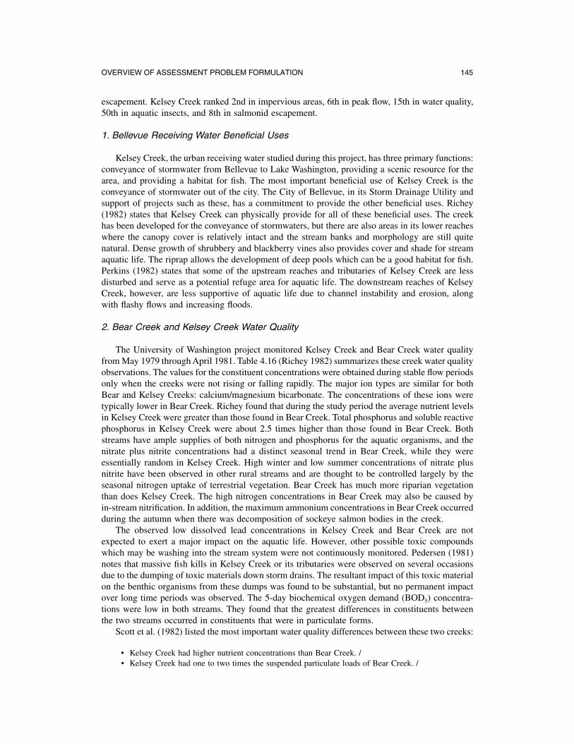
OVERVIEW OF ASSESSMENT PROBLEM FORMULATION 145
escapement. Kelsey Creek ranked 2nd in impervious areas, 6th in peak flow, 15th in water quality, 50th in aquatic insects, and 8th in salmonid escapement.
1. Bellevue Receiving Water Beneficial Uses
Kelsey Creek, the urban receiving water studied during this project, has three primary functions: conveyance of stormwater from Bellevue to Lake Washington, providing a scenic resource for the area, and providing a habitat for fish. The most important beneficial use of Kelsey Creek is the conveyance of stormwater out of the city. The City of Bellevue, in its Storm Drainage Utility and support of projects such as these, has a commitment to provide the other beneficial uses. Richey (1982) states that Kelsey Creek can physically provide for all of these beneficial uses. The creek has been developed for the conveyance of stormwaters, but there are also areas in its lower reaches where the canopy cover is relatively intact and the stream banks and morphology are still quite natural. Dense growth of shrubbery and blackberry vines also provides cover and shade for stream aquatic life. The riprap allows the development of deep pools which can be a good habitat for fish. Perkins (1982) states that some of the upstream reaches and tributaries of Kelsey Creek are less disturbed and serve as a potential refuge area for aquatic life. The downstream reaches of Kelsey Creek, however, are less supportive of aquatic life due to channel instability and erosion, along with flashy flows and increasing floods.
2. Bear Creek and Kelsey Creek Water Quality
The University of Washington project monitored Kelsey Creek and Bear Creek water quality from May 1979 through April 1981. Table 4.16 (Richey 1982) summarizes these creek water quality observations. The values for the constituent concentrations were obtained during stable flow periods only when the creeks were not rising or falling rapidly. The major ion types are similar for both Bear and Kelsey Creeks: calcium/magnesium bicarbonate. The concentrations of these ions were typically lower in Bear Creek. Richey found that during the study period the average nutrient levels in Kelsey Creek were greater than those found in Bear Creek. Total phosphorus and soluble reactive phosphorus in Kelsey Creek were about 2.5 times higher than those found in Bear Creek. Both streams have ample supplies of both nitrogen and phosphorus for the aquatic organisms, and the nitrate plus nitrite concentrations had a distinct seasonal trend in Bear Creek, while they were essentially random in Kelsey Creek. High winter and low summer concentrations of nitrate plus nitrite have been observed in other rural streams and are thought to be controlled largely by the seasonal nitrogen uptake of terrestrial vegetation. Bear Creek has much more riparian vegetation than does Kelsey Creek. The high nitrogen concentrations in Bear Creek may also be caused by in-stream nitrification. In addition, the maximum ammonium concentrations in Bear Creek occurred during the autumn when there was decomposition of sockeye salmon bodies in the creek.
The observed low dissolved lead concentrations in Kelsey Creek and Bear Creek are not expected to exert a major impact on the aquatic life. However, other possible toxic compounds which may be washing into the stream system were not continuously monitored. Pedersen (1981) notes that massive fish kills in Kelsey Creek or its tributaries were observed on several occasions due to the dumping of toxic materials down storm drains. The resultant impact of this toxic material on the benthic organisms from these dumps was found to be substantial, but no permanent impact over long time periods was observed. The 5-day biochemical oxygen demand (BOD5) concentra- tions were low in both streams. They found that the greatest differences in constituents between the two streams occurred in constituents that were in particulate forms.
Scott et al. (1982) listed the most important water quality differences between these two creeks:
• Kelsey Creek had higher nutrient concentrations than Bear Creek. /• Kelsey Creek had one to two times the suspended particulate loads of Bear Creek. /
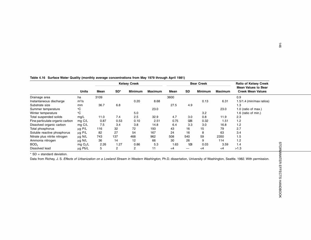
146 S
TOR
MW
ATE
R E
FF
EC
TS
HA
ND
BO
OK
Table 4.16 Surface Water Quality (monthly average concentrations from May 1979 through April 1981)
Kelsey Creek Bear Creek Ratio of Kelsey Creek Mean Values to Bear
Units Mean SD* Minimum Maximum Mean SD Minimum Maximum Creek Mean Values
Drainage area ha 3109 3600 0.9Instantaneous discharge m3/s 0.20 8.68 0.13 6.31 1.5/1.4 (min/max ratios) Substrate size mm 36.7 6.8 27.5 4.9 1.3Summer temperature oC 23.0 23.0 1.0 (ratio of max.) Winter temperature oC 5.0 3.2 1.6 (ratio of min.) Total suspended solids mg/L 11.0 7.4 2.5 32.9 4.7 3.0 0.8 11.9 2.3Fine particulate organic carbon mg C/L 0.87 0.53 0.10 2.51 0.75 0.36 0.32 1.51 1.2Dissolved organic carbon mg C/L 7.5 3.4 3.8 14.8 6.4 3.3 3.0 16.8 1.2Total phosphorus µg P/L 116 32 72 193 43 16 15 79 2.7Soluble reactive phosphorus µg P/L 82 27 54 167 24 16 8 63 3.4Nitrate plus nitrite nitrogen µg N/L 743 137 468 962 508 540 59 2350 1.5Ammonia nitrogen µg N/L 36 14 12 66 30 26 9 114 1.2BOD5 mg O2/L 2.26 1.27 0.86 5.3 1.63 1.08 0.03 3.59 1.4Dissolved lead µg Pb/L 5 2 2 11 <4 — <4 <4 >1.3
* SD = standard deviation.
Data from Richey, J. S. Effects of Urbanization on a Lowland Stream in Western Washington, Ph.D. dissertation, University of Washington, Seattle. 1982. With permission.
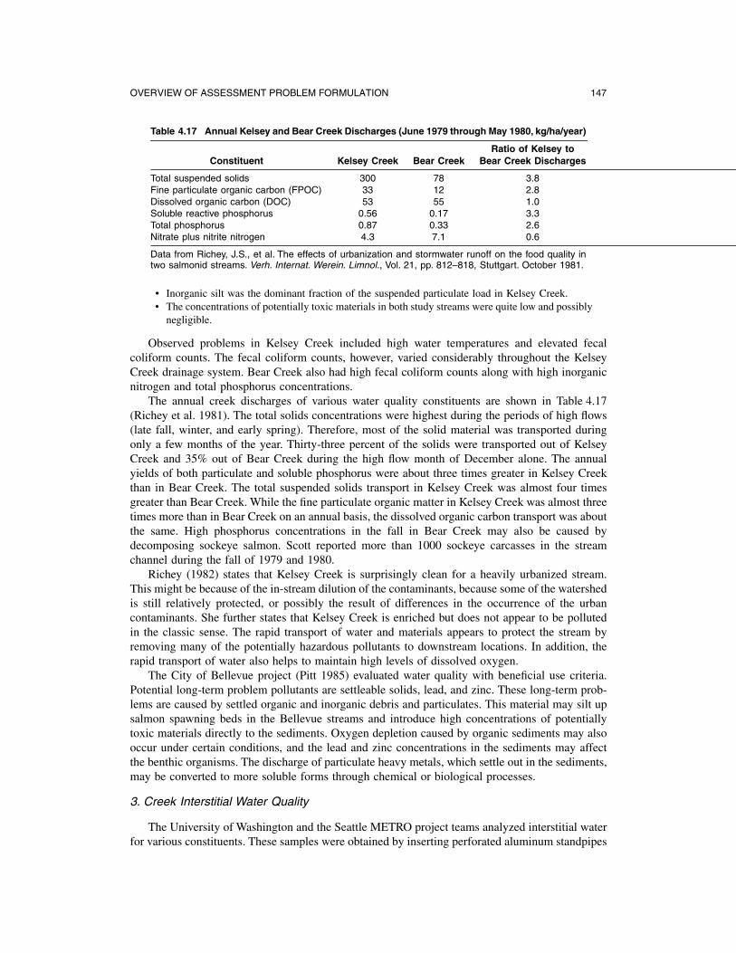
OVERVIEW OF ASSESSMENT PROBLEM FORMULATION 147
Table 4.17 Annual Kelsey and Bear Creek Discharges (June 1979 through May 1980, kg/ha/year)
Ratio of Kelsey to Constituent Kelsey Creek Bear Creek Bear Creek Discharges
Total suspended solids 300 78 3.8 Fine particulate organic carbon (FPOC) 33 12 2.8 Dissolved organic carbon (DOC) 53 55 1.0 Soluble reactive phosphorus 0.56 0.17 3.3 Total phosphorus 0.87 0.33 2.6 Nitrate plus nitrite nitrogen 4.3 7.1 0.6
Data from Richey, J.S., et al. The effects of urbanization and stormwater runoff on the food quality in two salmonid streams. Verh. Internat. Werein. Limnol., Vol. 21, pp. 812–818, Stuttgart. October 1981.
• Inorganic silt was the dominant fraction of the suspended particulate load in Kelsey Creek. • The concentrations of potentially toxic materials in both study streams were quite low and possibly
negligible.
Observed problems in Kelsey Creek included high water temperatures and elevated fecal coliform counts. The fecal coliform counts, however, varied considerably throughout the Kelsey Creek drainage system. Bear Creek also had high fecal coliform counts along with high inorganic nitrogen and total phosphorus concentrations.
The annual creek discharges of various water quality constituents are shown in Table 4.17 (Richey et al. 1981). The total solids concentrations were highest during the periods of high flows (late fall, winter, and early spring). Therefore, most of the solid material was transported during only a few months of the year. Thirty-three percent of the solids were transported out of Kelsey Creek and 35% out of Bear Creek during the high flow month of December alone. The annual yields of both particulate and soluble phosphorus were about three times greater in Kelsey Creek than in Bear Creek. The total suspended solids transport in Kelsey Creek was almost four times greater than Bear Creek. While the fine particulate organic matter in Kelsey Creek was almost three times more than in Bear Creek on an annual basis, the dissolved organic carbon transport was about the same. High phosphorus concentrations in the fall in Bear Creek may also be caused by decomposing sockeye salmon. Scott reported more than 1000 sockeye carcasses in the stream channel during the fall of 1979 and 1980.
Richey (1982) states that Kelsey Creek is surprisingly clean for a heavily urbanized stream. This might be because of the in-stream dilution of the contaminants, because some of the watershed is still relatively protected, or possibly the result of differences in the occurrence of the urban contaminants. She further states that Kelsey Creek is enriched but does not appear to be polluted in the classic sense. The rapid transport of water and materials appears to protect the stream by removing many of the potentially hazardous pollutants to downstream locations. In addition, the rapid transport of water also helps to maintain high levels of dissolved oxygen.
The City of Bellevue project (Pitt 1985) evaluated water quality with beneficial use criteria. Potential long-term problem pollutants are settleable solids, lead, and zinc. These long-term problems are caused by settled organic and inorganic debris and particulates. This material may silt up salmon spawning beds in the Bellevue streams and introduce high concentrations of potentially toxic materials directly to the sediments. Oxygen depletion caused by organic sediments may also occur under certain conditions, and the lead and zinc concentrations in the sediments may affect the benthic organisms. The discharge of particulate heavy metals, which settle out in the sediments, may be converted to more soluble forms through chemical or biological processes.
3. Creek Interstitial Water Quality
The University of Washington and the Seattle METRO project teams analyzed interstitial water for various constituents. These samples were obtained by inserting perforated aluminum standpipes

148 STORMWATER EFFECTS HANDBOOK
into the creek sediment. This water is most affected by the sediment quality and in turn affects the benthic organisms much more than the creek water column. Scott et al. (1982) found that the interstitial water pH ranged from 6.5 to 7.6 and did not significantly differ between the two streams but did tend to decrease during the spring months. The lower fall temperatures and pH levels contributed to reductions in ammonium concentrations. The total ammonia and ammonium concentrations were significantly greater in Kelsey Creek than in Bear Creek. They also found that the interstitial dissolved oxygen concentrations in Kelsey Creek were much below concentrations considered normal for undisturbed watersheds. These decreased interstitial oxygen concentrations were much less than the water column concentrations and indicated the possible impact of urban development. The dissolved oxygen concentrations in the interstitial waters and Bear Creek were also lower than expected, potentially suggesting deteriorating fish spawning conditions. During the winter and spring months, the interstitial oxygen concentrations appeared to be intermediate between those characteristic of disturbed and undisturbed watersheds.
The University of Washington (Richey 1982) also analyzed heavy metals in the interstitial waters. They found that copper and chromium concentrations were very low or undetectable, while lead and zinc were higher. Kelsey Creek interstitial water also had concentrations approximately twice those found in the Bear Creek interstitial water. They expect that most of the metals were loosely bound to fine sediment particles. Most of the lead was associated with the particulates and very little soluble lead was found in the interstitial waters. The interstitial samples taken from the standpipes were full of sediment particles that could be expected to release lead into solution following the mild acid digestion for exchangeable lead analyses. They also found that the metal concentrations in Kelsey Creek interstitial water decreased in a downstream direction. They felt that this might be caused by stream scouring of the benthic material in that part of the creek. The downstream Kelsey Creek sites were more prone to erosion and channel scouring, while the most upstream station was relatively stable.
Seattle METRO (Galvin and Moore 1982) also monitored heavy metals in the interstitial waters in Kelsey and Bear Creeks. They found large variations in heavy metal concentrations depending upon whether the sample was obtained during the wet or the dry season. During storm periods, the interstitial water and creek water heavy metal concentrations approached the stormwater values (200 µg/L for lead). During nonstorm periods, the interstitial lead concentrations were typically only about 1 µg/L. They also analyzed priority pollutant organics in interstitial waters. Only benzene was found and only in the urban stream. The observed benzene concentrations in two Kelsey Creek samples were 22 and 24 µg/L, while the reported concentrations were less than 1 µg/L in all other interstitial water samples analyzed for benzene.
4. Increased Kelsey Creek Water Flows
The increasing population of the City of Bellevue and the observed peak annual discharges have been studied by the University of Washington (Richey 1982). Bellevue was initially settled in 1883 but it grew slowly, reaching a population of only 400 by 1900. The Bellevue population density continued to be low until the 1940s. During this time, almost the entire Kelsey Creek drainage basin was undeveloped. In the late 1940s, the City of Bellevue’s population was stimulated by the construction of the Lake Washington floating bridge connecting Bellevue to Seattle. From 1950 to 1970, low-density residential housing progressed rapidly, and the population of the greater Bellevue area increased by nearly 600%. By 1959, residential housing occupied a substantial portion of the Kelsey Creek watershed. The Bellevue population slowed during the 1970s due to the depressed local economy and the saturation of land development. In 1976, the population of the City of Bellevue was estimated to be 67,000 people. The peak annual discharges of Kelsey Creek almost doubled between the 1950s and the late 1970s. The frequency of flooding during this period of time also increased. Floods that used to return every 10 years in the early 1950s returned at least every other year during the late 1970s. The increase in the rate of runoff has also had a measurable effect on the channel stability in Kelsey Creek.