compressible flow - tme085 - lecture 10 - chalmersnian/courses/compflow/notes/tme085_l10.pdf ·...
TRANSCRIPT

Compressible Flow - TME085
Lecture 10
Niklas Andersson
Chalmers University of Technology
Department of Mechanics and Maritime Sciences
Division of Fluid Mechanics
Gothenburg, Sweden

Adressed Learning Outcomes
3 Describe typical engineering flow situations in which
compressibility effects are more or less predominant (e.g.
Mach number regimes for steady-state flows)
8 Derive (marked) and apply (all) of the presentedmathematical formulae for classical gas dynamics
j unsteady waves and discontinuities in 1D
9 Solve engineering problems involving the above-mentioned
phenomena (8a-8k)
12 Explain the main principles behind a modern Finite Volume
CFD code and such concepts as explicit/implicit time
stepping, CFL number, conservation, handling of
compression shocks, and boundary conditions
Niklas Andersson - Chalmers 2 / 43

Chapter 7
Unsteady Wave Motion
Niklas Andersson - Chalmers 3 / 43

Unsteady Wave Motion
I Moving normal shocks
I Shock tube/shock tunnel
I Acoustic theory (sound waves)
I Finite (non-linear) waves
Niklas Andersson - Chalmers 4 / 43

Chapter 7.2
Moving Normal Shock
Waves
Niklas Andersson - Chalmers 5 / 43
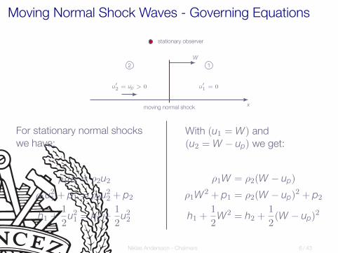
Moving Normal Shock Waves - Governing Equations
2 1
stationary observer
u′2 = up > 0 u
′1 = 0
x
W
moving normal shock
For stationary normal shocks
we have:
With (u1 = W) and(u2 = W − up) we get:
ρ1u1 = ρ2u2
ρ1u21 + p1 = ρ2u
22 + p2
h1 +1
2u21 = h2 +
1
2u22
ρ1W = ρ2(W − up)
ρ1W2 + p1 = ρ2(W − up)
2 + p2
h1 +1
2W2 = h2 +
1
2(W − up)
2
Niklas Andersson - Chalmers 6 / 43

Moving Normal Shock Waves - Relations cont.
From the continuity equation we get:
up = W
(1− ρ1
ρ2
)> 0
After some derivation we obtain:
up =a1
γ
(p2
p1− 1
)2γ
γ + 1p2
p1+
γ − 1
γ + 1
1/2
Niklas Andersson - Chalmers 7 / 43

Moving Normal Shock Waves - Relations cont.
May also show that
ρ2ρ1
=
1 +γ + 1
γ − 1
(p2
p1
)γ + 1
γ − 1+
p2
p1
and
T2
T1=
p2
p1
γ + 1
γ − 1+
p2
p1
1 +γ + 1
γ − 1
(p2
p1
)
Niklas Andersson - Chalmers 8 / 43
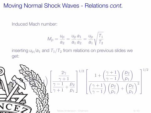
Moving Normal Shock Waves - Relations cont.
Induced Mach number:
Mp =up
a2=
up
a1
a1
a2=
up
a1
√T1
T2
inserting up/a1 and T1/T2 from relations on previous slides we
get:
Mp =1
γ
(p2
p1− 1
)2γ
γ + 1γ − 1
γ + 1+
p2
p1
1/2
1 +
(γ + 1
γ − 1
)(p2
p1
)(γ + 1
γ − 1
)(p2
p1
)+
(p2
p1
)2
1/2
Niklas Andersson - Chalmers 9 / 43

Moving Normal Shock Waves - Relations cont.
Not that
limp2p1
→∞Mp →
√2
γ(γ − 1)
for air (γ = 1.4)
limp2p1
→∞Mp → 1.89
Niklas Andersson - Chalmers 10 / 43

Moving Normal Shock Waves - Relations cont.
Note that ho1 6= ho2
constant total enthalpy is only valid for stationary shocks!
shock is uniquely defined by pressure ratio p2/p1
u1 = 0
ho1 = h1 +1
2u21 = h1
ho2 = h2 +1
2u22
h2 > h1 ⇒ ho2 > ho12 4 6 8 10
1.1
1.2
1.3
1.4
1.5
1.6
1.7
1.8
1.9
2
1.5
2
2.5
3
3.5
4
p2/p1
T2/T1 = h2/h1 (if Cp is constant)
γ
Niklas Andersson - Chalmers 11 / 43

Moving Normal Shock Waves - Relations cont.
Gas/Vapor Ratio of specific heats Gas constant
(γ) R
Acetylene 1.23 319
Air (standard) 1.40 287
Ammonia 1.31 530
Argon 1.67 208
Benzene 1.12 100
Butane 1.09 143
Carbon Dioxide 1.29 189
Carbon Disulphide 1.21 120
Carbon Monoxide 1.40 297
Chlorine 1.34 120
Ethane 1.19 276
Ethylene 1.24 296
Helium 1.67 2080
Hydrogen 1.41 4120
Hydrogen chloride 1.41 230
Methane 1.30 518
Natural Gas (Methane) 1.27 500
Nitric oxide 1.39 277
Nitrogen 1.40 297
Nitrous oxide 1.27 180
Oxygen 1.40 260
Propane 1.13 189
Steam (water) 1.32 462
Sulphur dioxide 1.29 130
Niklas Andersson - Chalmers 12 / 43

The Shock Tube
Niklas Andersson - Chalmers 13 / 43

Shock Tube
p
x
p4
p1
4 1
diaphragm
diaphragm location
tube with closed ends
diaphragm inside, separating two differ-
ent constant states
(could also be two different gases)
if diaphragm is removed suddenly (by
inducing a breakdown) the two states
come into contact and a flow develops
assume that p4 > p1:
state 4 is ”driver” section
state 1 is ”driven” section
Niklas Andersson - Chalmers 14 / 43

Shock Tube
t
x
dx
dt= W
dx
dt= up
4
3 2
1
4 3 2 1
Wup
expansion fan contact discontinuity moving normal shock
diaphragm location
flow at some time after diaphragm
breakdown
Niklas Andersson - Chalmers 14 / 43

Shock Tube
p
x
p4
p3 p2
p1
(p3 = p2)
4 3 2 1
Wup
expansion fan contact discontinuity moving normal shock
diaphragm location
flow at some time after diaphragm
breakdown
Niklas Andersson - Chalmers 14 / 43

Shock Tube cont.
I By using light gases for the driver section (e.g. He) and
heavier gases for the driven section (e.g. air) the pressure p4required for a specific p2/p1 ratio is significantly reduced
I If T4/T1 is increased, the pressure p4 required for a specific
p2/p1 is also reduced
Niklas Andersson - Chalmers 15 / 43

Riemann Problem
The shock tube problem is a special case of the general Riemann
Problem
”… A Riemann problem, named after Bernhard
Riemann, consists of an initial value problem composed
by a conservation equation together with piecewise
constant data having a single discontinuity …”
Wikipedia
Niklas Andersson - Chalmers 16 / 43

Riemann Problem cont.
May show that solutions to the shock tube problem have the
general form:
p = p(x/t)
ρ = ρ(x/t)
u = u(x/t)
T = T(x/t)
a = a(x/t)
where x = 0 denotes theposition of the initial ”jump”
between states 1 and 4
Niklas Andersson - Chalmers 17 / 43

Riemann Problem - Shock Tube
Shock tube simulation:
I left side conditions (state 4):
I ρ = 2.4 kg/m3
I u = 0.0 m/sI p = 2.0 bar
I right side conditions (state 1):
I ρ = 1.2 kg/m3
I u = 0.0 m/sI p = 1.0 bar
I Numerical method
I Finite-Volume Method (FVM) solverI three-stage Runge-Kutta time steppingI third-order characteristic upwinding schemeI local artificial damping
Niklas Andersson - Chalmers 18 / 43

Riemann Problem - Shock Tube cont.
0 0.5 1 1.5 2 2.5 31
1.5
2
2.5
0 0.5 1 1.5 2 2.5 31
1.5
2
2.5
0 0.5 1 1.5 2 2.5 31
1.5
2
2.5
density
0 0.5 1 1.5 2 2.5 3−20
0
20
40
60
80
100
0 0.5 1 1.5 2 2.5 3−20
0
20
40
60
80
100
0 0.5 1 1.5 2 2.5 3−20
0
20
40
60
80
100
velocity
0 0.5 1 1.5 2 2.5 30
0.5
1
1.5
2
2.5x 10
5
0 0.5 1 1.5 2 2.5 30
0.5
1
1.5
2
2.5x 10
5
0 0.5 1 1.5 2 2.5 30
0.5
1
1.5
2
2.5x 10
5
pressure
t = 0.0000 s t = 0.0010 s t = 0.0025 s
Niklas Andersson - Chalmers 19 / 43

Riemann Problem - Shock Tube cont.
0 0.5 1 1.5 2 2.5 31
1.5
2
2.5
0 0.5 1 1.5 2 2.5 31
1.5
2
2.5
0 0.5 1 1.5 2 2.5 31
1.5
2
2.5
density
0 0.5 1 1.5 2 2.5 3−20
0
20
40
60
80
100
0 0.5 1 1.5 2 2.5 3−20
0
20
40
60
80
100
0 0.5 1 1.5 2 2.5 3−20
0
20
40
60
80
100
velocity
0 0.5 1 1.5 2 2.5 30
0.5
1
1.5
2
2.5x 10
5
0 0.5 1 1.5 2 2.5 30
0.5
1
1.5
2
2.5x 10
5
0 0.5 1 1.5 2 2.5 30
0.5
1
1.5
2
2.5x 10
5
pressure
t = 0.0000 s t = 0.0010 s t = 0.0025 s
expansion fan
contact discontinuity
moving shock wave
Niklas Andersson - Chalmers 19 / 43

Riemann Problem - Shock Tube cont.
−2000 −1500 −1000 −500 0 500 1000 1500 20001
1.5
2
2.5
x/t [m/s]
ρ[kg/m3]
density {ρ = ρ(x/t)}
t = 0.0010 s
t = 0.0025 s
Niklas Andersson - Chalmers 20 / 43

Riemann Problem - Shock Tube cont.
−2000 −1500 −1000 −500 0 500 1000 1500 2000−20
0
20
40
60
80
100
x/t [m/s]
u[m
/s]
velocity {u = u(x/t)}
t = 0.0010 s
t = 0.0025 s
Niklas Andersson - Chalmers 21 / 43

Riemann Problem - Shock Tube cont.
−2000 −1500 −1000 −500 0 500 1000 1500 20000
0.5
1
1.5
2
2.5x 10
5
x/t [m/s]
p[Pa]
pressure {p = p(x/t)}
t = 0.0010 s
t = 0.0025 s
Niklas Andersson - Chalmers 22 / 43

Chapter 7.3
Reflected Shock Wave
Niklas Andersson - Chalmers 23 / 43

Shock Reflection
x
t
1
5
2
3
initial moving shock,dx
dt= W
reflected shock,dx
dt= −Wr
contact surface,dx
dt= up
contact surface,dx
dt= 0
solid wall
Niklas Andersson - Chalmers 24 / 43

Shock Reflection - Particle Path
A fluid particle located at x0 at time t0 (a location ahead of the
shock) will be affected by the moving shock and follow the blue
path
time location velocity
t0 x0 0t1 x0 upt2 x1 upt3 x1 0
x
t
x0 x1t0
t1
t2
t3
Niklas Andersson - Chalmers 25 / 43

Shock Reflection Relations
I velocity ahead of reflected shock: Wr + up
I velocity behind reflected shock: Wr
Continuity:
ρ2(Wr + up) = ρ5Wr
Momentum:
p2 + ρ2(Wr + up)2 = p5 + ρ5W
2r
Energy:
h2 +1
2(Wr + up)
2 = h5 +1
2W2
r
Niklas Andersson - Chalmers 26 / 43

Shock Reflection Relations
Reflected shock is determined such that u5 = 0
Mr
M2r − 1
=Ms
M2s − 1
√1 +
2(γ − 1)
(γ + 1)2(M2
s − 1)
(γ +
1
M2s
)
where
Mr =Wr + up
a2
Niklas Andersson - Chalmers 27 / 43

Tailored v.s. Non-Tailored Shock Reflection
I The time duration of condition 5 is determined by what
happens after interaction between reflected shock and
contact discontinuity
I For special choice of initial conditions (tailored case), this
interaction is negligible, thus prolonging the duration of
condition 5
Niklas Andersson - Chalmers 28 / 43

Tailored v.s. Non-Tailored Shock Reflection
5
1
2
3
t
x
wall
under-tailored
5
1
2
3
t
x
wall
tailored
5
1
2
3
t
x
wall
over-tailored
shock wave
contact surface
expansion wave
I Under-tailored conditions: Mach number of incident wave
lower than in tailored conditions
I Over-tailored conditions: Mach number of incident wave
higher than in tailored conditions
Niklas Andersson - Chalmers 29 / 43

Shock Reflection - Example
Shock reflection in shock tube (γ = 1.4)(Example 7.1 in Anderson)
Incident shock (given data)
p2/p1 10.0
Ms 2.95
T2/T1 2.623
p1 1.0 [bar]
T1 300.0 [K]
Calculated data
Mr 2.09
Table A.2
p5/p2 4.978
T5/T2 1.77
p5 =
(p5
p2
)(p2
p1
)p1 = 49.78
T5 =
(T5
T2
)(T2
T1
)T1 = 1393
Niklas Andersson - Chalmers 30 / 43

Shock Reflection - Shock Tube
I Very high pressure and temperature conditions in a specified
location with very high precision (p5,T5)
I measurements of thermodynamic properties of various gases
at extreme conditions, e.g. dissociation energies, molecular
relaxation times, etc.
I measurements of chemical reaction properties of various gas
mixtures at extreme conditions
Niklas Andersson - Chalmers 31 / 43

Shock Tunnel
I Addition of a convergent-divergent nozzle to a shock tube
configuration
I Capable of producing flow conditions which are close tothose during the reentry of a space vehicles into the earth’satmosphere
I high-enthalpy, hypersonic flows (short time)I real gas effects
I Example - Aachen TH2:
I velocities up to 4 km/sI stagnation temperatures of several thousand degrees
Niklas Andersson - Chalmers 32 / 43

Shock Tunnel cont.
driver section driven section
test section
dump tank
Wr
diaphragm 2diaphragm 1
reflected shock
test object
1. High pressure in region 4 (driver section)
I diaphragm 1 burstI primary shock generated
2. Primary shock reaches end of shock tube
I shock reflection
3. High pressure in region 5
I diaphragm 2 burstI nozzle flow initiatedI hypersonic flow in test section
Niklas Andersson - Chalmers 33 / 43

Shock Tunnel cont.
reflected expansion fan
incident shock wave
reflected shock wave
contact surface
1
2
3
4
5
t
x
4 1
driver section driven section
diaphragm location wall
Niklas Andersson - Chalmers 34 / 43

Shock Tunnel cont.
By adding a compression tube to the shock tube a very high p4and T4 may be achieved for any gas in a fairly simple manner
heavy piston compression tube diaphragm
pressurized airdriver gas
p, T
driven gas
p1, T1
pressurized airdriver gas
p4, T4
driven gas
p1, T1
Niklas Andersson - Chalmers 35 / 43
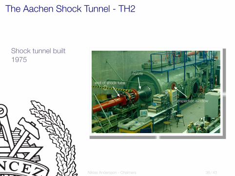
The Aachen Shock Tunnel - TH2
Shock tunnel built
1975
nozzle
end of shock tube
inspection window
Niklas Andersson - Chalmers 36 / 43

The Aachen Shock Tunnel - TH2
Shock tube specifications:
diameter 140 mm
driver section 6.0 m
driven section 15.4 m
diaphragm 1 10 mm stainless steel
diaphragm 2 copper/brass sheet
max operating (steady) pressure 1500 bar
Niklas Andersson - Chalmers 37 / 43

The Aachen Shock Tunnel - TH2
I Driver gas (usually helium):
I 100 bar < p4 < 1500 barI electrical preheating (optional) to 600 K
I Driven gas:
I 0.1 bar < p1 < 10 bar
I Dump tank evacuated before test
Niklas Andersson - Chalmers 38 / 43

The Aachen Shock Tunnel - TH2
initial conditions shock reservoir free stream
p4 T4 p1 Ms p2 p5 T5 M∞ T∞ u∞ p∞[bar] [K] [bar] [bar] [bar] [K] [K] [m/s] [mbar]
100 293 1.0 3.3 12 65 1500 7.7 125 1740 7.6
370 500 1.0 4.6 26 175 2500 7.4 250 2350 20.0
720 500 0.7 5.6 50 325 3650 6.8 460 3910 42.0
1200 500 0.6 6.8 50 560 4600 6.5 700 3400 73.0
100 293 0.9 3.4 12 65 1500 11.3 60 1780 0.6
450 500 1.2 4.9 29 225 2700 11.3 120 2480 1.5
1300 520 0.7 6.4 46 630 4600 12.1 220 3560 1.2
26 293 0.2 3.4 12 15 1500 11.4 60 1780 0.1
480 500 0.2 6.6 50 210 4600 11.0 270 3630 0.7
100 293 1.0 3.4 12 65 1500 7.7 130 1750 7.3
370 500 1.0 5.1 27 220 2700 7.3 280 2440 26.3
Niklas Andersson - Chalmers 39 / 43

The Caltech Shock Tunnel - T5
Free-piston shock tunnel
Niklas Andersson - Chalmers 40 / 43

The Caltech Shock Tunnel - T5 cont.
I Compression tube (CT):
I length 30 m, diameter 300 mmI free piston (120 kg)I max piston velocity: 300 m/sI driven by compressed air (80 bar - 150 bar)
I Shock tube (ST):
I length 12 m, diameter 90 mmI driver gas: helium + argonI driven gas: airI diaphragm 1: 7 mm stainless steelI p4 max 1300 bar
Niklas Andersson - Chalmers 41 / 43

The Caltech Shock Tunnel - T5 cont.
I Reservoir conditions:
I p5 1000 barI T5 10000 K
I Freestream conditions (design conditions):
I M∞ 5.2I T∞ 2000 KI p∞ 0.3 barI typical test time 1 ms
Niklas Andersson - Chalmers 42 / 43

Other Examples of Shock Tunnels
Niklas Andersson - Chalmers 43 / 43