compressible flow
TRANSCRIPT

Fundamentals of CompressibleFluid Mechanics
Genick Bar–Meir, Ph. D.
1107 16th Ave S. E.Minneapolis, MN 55414-2411email: “[email protected]”
Copyright © 2007, 2006, 2005, and 2004 by Genick Bar-MeirSee the file copying.fdl or copyright.tex for copying conditions.
Version (0.4.8.5 January 13, 2009)

‘We are like dwarfs sitting on the shoulders of giants”
from The Metalogicon by John in 1159

CONTENTS
Nomenclature xvFeb-21-2007 version . . . . . . . . . . . . . . . . . . . . . . . . . . xix
Jan-16-2007 version . . . . . . . . . . . . . . . . . . . . . . . . . . . xixDec-04-2006 version . . . . . . . . . . . . . . . . . . . . . . . . . . xx
GNU Free Documentation License . . . . . . . . . . . . . . . . . . . . . . xxiii1. APPLICABILITY AND DEFINITIONS . . . . . . . . . . . . . . . . xxiv2. VERBATIM COPYING . . . . . . . . . . . . . . . . . . . . . . . . xxv3. COPYING IN QUANTITY . . . . . . . . . . . . . . . . . . . . . . . xxvi4. MODIFICATIONS . . . . . . . . . . . . . . . . . . . . . . . . . . . xxvi5. COMBINING DOCUMENTS . . . . . . . . . . . . . . . . . . . . . xxviii6. COLLECTIONS OF DOCUMENTS . . . . . . . . . . . . . . . . . xxix7. AGGREGATION WITH INDEPENDENT WORKS . . . . . . . . . xxix8. TRANSLATION . . . . . . . . . . . . . . . . . . . . . . . . . . . . xxix9. TERMINATION . . . . . . . . . . . . . . . . . . . . . . . . . . . . xxix10. FUTURE REVISIONS OF THIS LICENSE . . . . . . . . . . . . . xxxADDENDUM: How to use this License for your documents . . . . . . xxx
How to contribute to this book . . . . . . . . . . . . . . . . . . . . . . . . xxxiCredits . . . . . . . . . . . . . . . . . . . . . . . . . . . . . . . . . . . . . xxxi
John Martones . . . . . . . . . . . . . . . . . . . . . . . . . . . . . . xxxiGrigory Toker . . . . . . . . . . . . . . . . . . . . . . . . . . . . . . . xxxiiRalph Menikoff . . . . . . . . . . . . . . . . . . . . . . . . . . . . . . xxxiiDomitien Rataaforret . . . . . . . . . . . . . . . . . . . . . . . . . . xxxii
Gary Settles . . . . . . . . . . . . . . . . . . . . . . . . . . . . . . . . xxxiiYour name here . . . . . . . . . . . . . . . . . . . . . . . . . . . . . xxxiiTypo corrections and other ”minor” contributions . . . . . . . . . . . xxxiii
Version 0.4.8 Jan. 23, 2008 . . . . . . . . . . . . . . . . . . . . . . . . . . xliii
iii
iv CONTENTS
Version 0.4.3 Sep. 15, 2006 . . . . . . . . . . . . . . . . . . . . . . . . . . xliiiVersion 0.4.2 . . . . . . . . . . . . . . . . . . . . . . . . . . . . . . . . . . xlivVersion 0.4 . . . . . . . . . . . . . . . . . . . . . . . . . . . . . . . . . . . xlvVersion 0.3 . . . . . . . . . . . . . . . . . . . . . . . . . . . . . . . . . . . xlvVersion 0.5 . . . . . . . . . . . . . . . . . . . . . . . . . . . . . . . . . . . liVersion 0.4.3 . . . . . . . . . . . . . . . . . . . . . . . . . . . . . . . . . . liiVersion 0.4.1.7 . . . . . . . . . . . . . . . . . . . . . . . . . . . . . . . . . lii
Speed of Sound . . . . . . . . . . . . . . . . . . . . . . . . . . . . . lviStagnation effects . . . . . . . . . . . . . . . . . . . . . . . . . . . . lviNozzle . . . . . . . . . . . . . . . . . . . . . . . . . . . . . . . . . . lviNormal Shock . . . . . . . . . . . . . . . . . . . . . . . . . . . . . . . lviIsothermal Flow . . . . . . . . . . . . . . . . . . . . . . . . . . . . . . lviFanno Flow . . . . . . . . . . . . . . . . . . . . . . . . . . . . . . . . lviiRayleigh Flow . . . . . . . . . . . . . . . . . . . . . . . . . . . . . . . lviiEvacuation and filling semi rigid Chambers . . . . . . . . . . . . . . lviiEvacuating and filling chambers under external forces . . . . . . . . lviiOblique Shock . . . . . . . . . . . . . . . . . . . . . . . . . . . . . . lviiPrandtl–Meyer . . . . . . . . . . . . . . . . . . . . . . . . . . . . . . lviiTransient problem . . . . . . . . . . . . . . . . . . . . . . . . . . . . lvii
1 Introduction 11.1 What is Compressible Flow ? . . . . . . . . . . . . . . . . . . . . . . 11.2 Why Compressible Flow is Important? . . . . . . . . . . . . . . . . . 21.3 Historical Background . . . . . . . . . . . . . . . . . . . . . . . . . . 2
1.3.1 Early Developments . . . . . . . . . . . . . . . . . . . . . . . 41.3.2 The shock wave puzzle . . . . . . . . . . . . . . . . . . . . . 51.3.3 Choking Flow . . . . . . . . . . . . . . . . . . . . . . . . . . . 91.3.4 External flow . . . . . . . . . . . . . . . . . . . . . . . . . . . 131.3.5 Filling and Evacuating Gaseous Chambers . . . . . . . . . . 151.3.6 Biographies of Major Figures . . . . . . . . . . . . . . . . . . 15
2 Review of Thermodynamics 252.1 Basic Definitions . . . . . . . . . . . . . . . . . . . . . . . . . . . . . 25
3 Fundamentals of Basic Fluid Mechanics 333.1 Introduction . . . . . . . . . . . . . . . . . . . . . . . . . . . . . . . . 333.2 Fluid Properties . . . . . . . . . . . . . . . . . . . . . . . . . . . . . . 333.3 Control Volume . . . . . . . . . . . . . . . . . . . . . . . . . . . . . . 333.4 Reynold’s Transport Theorem . . . . . . . . . . . . . . . . . . . . . . 33
4 Speed of Sound 354.1 Motivation . . . . . . . . . . . . . . . . . . . . . . . . . . . . . . . . . 354.2 Introduction . . . . . . . . . . . . . . . . . . . . . . . . . . . . . . . . 354.3 Speed of sound in ideal and perfect gases . . . . . . . . . . . . . . . 374.4 Speed of Sound in Real Gas . . . . . . . . . . . . . . . . . . . . . . 39

CONTENTS v
4.5 Speed of Sound in Almost Incompressible Liquid . . . . . . . . . . . 434.6 Speed of Sound in Solids . . . . . . . . . . . . . . . . . . . . . . . . 444.7 Sound Speed in Two Phase Medium . . . . . . . . . . . . . . . . . . 45
5 Isentropic Flow 495.1 Stagnation State for Ideal Gas Model . . . . . . . . . . . . . . . . . . 49
5.1.1 General Relationship . . . . . . . . . . . . . . . . . . . . . . . 495.1.2 Relationships for Small Mach Number . . . . . . . . . . . . . 52
5.2 Isentropic Converging-Diverging Flow in Cross Section . . . . . . . . 535.2.1 The Properties in the Adiabatic Nozzle . . . . . . . . . . . . . 545.2.2 Isentropic Flow Examples . . . . . . . . . . . . . . . . . . . . 585.2.3 Mass Flow Rate (Number) . . . . . . . . . . . . . . . . . . . 61
5.3 Isentropic Tables . . . . . . . . . . . . . . . . . . . . . . . . . . . . . 705.3.1 Isentropic Isothermal Flow Nozzle . . . . . . . . . . . . . . . 725.3.2 General Relationship . . . . . . . . . . . . . . . . . . . . . . . 72
5.4 The Impulse Function . . . . . . . . . . . . . . . . . . . . . . . . . . 795.4.1 Impulse in Isentropic Adiabatic Nozzle . . . . . . . . . . . . 795.4.2 The Impulse Function in Isothermal Nozzle . . . . . . . . . . 82
5.5 Isothermal Table . . . . . . . . . . . . . . . . . . . . . . . . . . . . . 825.6 The effects of Real Gases . . . . . . . . . . . . . . . . . . . . . . . . 84
6 Normal Shock 896.1 Solution of the Governing Equations . . . . . . . . . . . . . . . . . . 92
6.1.1 Informal Model . . . . . . . . . . . . . . . . . . . . . . . . . . 926.1.2 Formal Model . . . . . . . . . . . . . . . . . . . . . . . . . . . 926.1.3 Prandtl’s Condition . . . . . . . . . . . . . . . . . . . . . . . . 96
6.2 Operating Equations and Analysis . . . . . . . . . . . . . . . . . . . 976.2.1 The Limitations of the Shock Wave . . . . . . . . . . . . . . . 986.2.2 Small Perturbation Solution . . . . . . . . . . . . . . . . . . . 986.2.3 Shock Thickness . . . . . . . . . . . . . . . . . . . . . . . . . 996.2.4 Shock or Wave Drag . . . . . . . . . . . . . . . . . . . . . . . 99
6.3 The Moving Shocks . . . . . . . . . . . . . . . . . . . . . . . . . . . 1006.3.1 Shock or Wave Drag Result from a Moving Shock . . . . . . 1036.3.2 Shock Result from a Sudden and Complete Stop . . . . . . . 1056.3.3 Moving Shock into Stationary Medium (Suddenly Open Valve) 1086.3.4 Partially Open Valve . . . . . . . . . . . . . . . . . . . . . . . 1176.3.5 Partially Closed Valve . . . . . . . . . . . . . . . . . . . . . . 1186.3.6 Worked–out Examples for Shock Dynamics . . . . . . . . . . 119
6.4 Shock Tube . . . . . . . . . . . . . . . . . . . . . . . . . . . . . . . . 1246.5 Shock with Real Gases . . . . . . . . . . . . . . . . . . . . . . . . . 1286.6 Shock in Wet Steam . . . . . . . . . . . . . . . . . . . . . . . . . . . 1286.7 Normal Shock in Ducts . . . . . . . . . . . . . . . . . . . . . . . . . . 1286.8 More Examples for Moving Shocks . . . . . . . . . . . . . . . . . . . 1296.9 Tables of Normal Shocks, k = 1.4 Ideal Gas . . . . . . . . . . . . . . 132

vi CONTENTS
7 Normal Shock in Variable Duct Areas 1397.1 Nozzle efficiency . . . . . . . . . . . . . . . . . . . . . . . . . . . . . 1457.2 Diffuser Efficiency . . . . . . . . . . . . . . . . . . . . . . . . . . . . 145
8 Nozzle Flow With External Forces 1518.1 Isentropic Nozzle (Q = 0) . . . . . . . . . . . . . . . . . . . . . . . . 1528.2 Isothermal Nozzle (T = constant) . . . . . . . . . . . . . . . . . . . 154
9 Isothermal Flow 1559.1 The Control Volume Analysis/Governing equations . . . . . . . . . . 1569.2 Dimensionless Representation . . . . . . . . . . . . . . . . . . . . . 1569.3 The Entrance Limitation of Supersonic Branch . . . . . . . . . . . . 1619.4 Comparison with Incompressible Flow . . . . . . . . . . . . . . . . . 1629.5 Supersonic Branch . . . . . . . . . . . . . . . . . . . . . . . . . . . . 1649.6 Figures and Tables . . . . . . . . . . . . . . . . . . . . . . . . . . . . 1659.7 Isothermal Flow Examples . . . . . . . . . . . . . . . . . . . . . . . . 1659.8 Unchoked situations in Fanno Flow . . . . . . . . . . . . . . . . . . . 170
10 Fanno Flow 17510.1 Introduction . . . . . . . . . . . . . . . . . . . . . . . . . . . . . . . . 17510.2 Fanno Model . . . . . . . . . . . . . . . . . . . . . . . . . . . . . . . 17610.3 Non–Dimensionalization of the Equations . . . . . . . . . . . . . . . 17710.4 The Mechanics and Why the Flow is Choked? . . . . . . . . . . . . . 18010.5 The Working Equations . . . . . . . . . . . . . . . . . . . . . . . . . 18110.6 Examples of Fanno Flow . . . . . . . . . . . . . . . . . . . . . . . . . 18510.7 Supersonic Branch . . . . . . . . . . . . . . . . . . . . . . . . . . . . 19010.8 Maximum Length for the Supersonic Flow . . . . . . . . . . . . . . . 19010.9 Working Conditions . . . . . . . . . . . . . . . . . . . . . . . . . . . 191
10.9.1 Variations of The Tube Length ( 4fLD ) Effects . . . . . . . . . . 192
10.9.2 The Pressure Ratio, P2P1
, effects . . . . . . . . . . . . . . . . . 19710.9.3 Entrance Mach number, M1, effects . . . . . . . . . . . . . . 199
10.10Practical Examples for Subsonic Flow . . . . . . . . . . . . . . . . . 20610.10.1Subsonic Fanno Flow for Given 4fL
D and Pressure Ratio . . . 20610.10.2Subsonic Fanno Flow for a Given M1 and Pressure Ratio . . 208
10.11The Approximation of the Fanno Flow by Isothermal Flow . . . . . . 21110.12More Examples of Fanno Flow . . . . . . . . . . . . . . . . . . . . . 21110.13The Table for Fanno Flow . . . . . . . . . . . . . . . . . . . . . . . . 21310.14Appendix . . . . . . . . . . . . . . . . . . . . . . . . . . . . . . . . . 214
11 Rayleigh Flow 21711.1 Introduction . . . . . . . . . . . . . . . . . . . . . . . . . . . . . . . . 21711.2 Governing Equation . . . . . . . . . . . . . . . . . . . . . . . . . . . 21811.3 Rayleigh Flow Tables . . . . . . . . . . . . . . . . . . . . . . . . . . . 22111.4 Examples For Rayleigh Flow . . . . . . . . . . . . . . . . . . . . . . 223

CONTENTS vii
12 Evacuating SemiRigid Chambers 23112.1 Governing Equations and Assumptions . . . . . . . . . . . . . . . . 23212.2 General Model and Non-dimensioned . . . . . . . . . . . . . . . . . 234
12.2.1 Isentropic Process . . . . . . . . . . . . . . . . . . . . . . . . 23612.2.2 Isothermal Process in The Chamber . . . . . . . . . . . . . . 23612.2.3 A Note on the Entrance Mach number . . . . . . . . . . . . . 236
12.3 Rigid Tank with Nozzle . . . . . . . . . . . . . . . . . . . . . . . . . . 23712.3.1 Adiabatic Isentropic Nozzle Attached . . . . . . . . . . . . . . 23712.3.2 Isothermal Nozzle Attached . . . . . . . . . . . . . . . . . . . 239
12.4 Rapid evacuating of a rigid tank . . . . . . . . . . . . . . . . . . . . 23912.4.1 With Fanno Flow . . . . . . . . . . . . . . . . . . . . . . . . . 23912.4.2 Filling Process . . . . . . . . . . . . . . . . . . . . . . . . . . 24112.4.3 The Isothermal Process . . . . . . . . . . . . . . . . . . . . . 24212.4.4 Simple Semi Rigid Chamber . . . . . . . . . . . . . . . . . . 24312.4.5 The “Simple” General Case . . . . . . . . . . . . . . . . . . . 243
12.5 Advance Topics . . . . . . . . . . . . . . . . . . . . . . . . . . . . . . 245
13 Evacuating under External Volume Control 24713.1 General Model . . . . . . . . . . . . . . . . . . . . . . . . . . . . . . 247
13.1.1 Rapid Process . . . . . . . . . . . . . . . . . . . . . . . . . . 24813.1.2 Examples . . . . . . . . . . . . . . . . . . . . . . . . . . . . . 25113.1.3 Direct Connection . . . . . . . . . . . . . . . . . . . . . . . . 251
13.2 Summary . . . . . . . . . . . . . . . . . . . . . . . . . . . . . . . . . 252
14 Oblique Shock 25514.1 Preface to Oblique Shock . . . . . . . . . . . . . . . . . . . . . . . . 25514.2 Introduction . . . . . . . . . . . . . . . . . . . . . . . . . . . . . . . . 256
14.2.1 Introduction to Oblique Shock . . . . . . . . . . . . . . . . . . 25614.2.2 Introduction to Prandtl–Meyer Function . . . . . . . . . . . . 25614.2.3 Introduction to Zero Inclination . . . . . . . . . . . . . . . . . 257
14.3 Oblique Shock . . . . . . . . . . . . . . . . . . . . . . . . . . . . . . 25714.4 Solution of Mach Angle . . . . . . . . . . . . . . . . . . . . . . . . . 260
14.4.1 Upstream Mach Number, M1, and Deflection Angle, δ . . . . 26014.4.2 When No Oblique Shock Exist or When D > 0 . . . . . . . . 26314.4.3 Upstream Mach Number, M1, and Shock Angle, θ . . . . . . 27114.4.4 Given Two Angles, δ and θ . . . . . . . . . . . . . . . . . . . 27314.4.5 Flow in a Semi–2D Shape . . . . . . . . . . . . . . . . . . . . 27414.4.6 Small δ “Weak Oblique shock” . . . . . . . . . . . . . . . . . 27614.4.7 Close and Far Views of the Oblique Shock . . . . . . . . . . 27714.4.8 Maximum Value of Oblique shock . . . . . . . . . . . . . . . . 277
14.5 Detached Shock . . . . . . . . . . . . . . . . . . . . . . . . . . . . . 27814.5.1 Issues Related to the Maximum Deflection Angle . . . . . . . 27914.5.2 Oblique Shock Examples . . . . . . . . . . . . . . . . . . . . 28114.5.3 Application of Oblique Shock . . . . . . . . . . . . . . . . . . 28314.5.4 Optimization of Suction Section Design . . . . . . . . . . . . 294

viii CONTENTS
14.5.5 Retouch of Shock or Wave Drag . . . . . . . . . . . . . . . . 29414.6 Summary . . . . . . . . . . . . . . . . . . . . . . . . . . . . . . . . . 29514.7 Appendix: Oblique Shock Stability Analysis . . . . . . . . . . . . . . 296
15 Prandtl-Meyer Function 29915.1 Introduction . . . . . . . . . . . . . . . . . . . . . . . . . . . . . . . . 29915.2 Geometrical Explanation . . . . . . . . . . . . . . . . . . . . . . . . . 300
15.2.1 Alternative Approach to Governing Equations . . . . . . . . . 30115.2.2 Comparison And Limitations between the Two Approaches . 305
15.3 The Maximum Turning Angle . . . . . . . . . . . . . . . . . . . . . . 30515.4 The Working Equations for the Prandtl-Meyer Function . . . . . . . . 30615.5 d’Alembert’s Paradox . . . . . . . . . . . . . . . . . . . . . . . . . . 30615.6 Flat Body with an Angle of Attack . . . . . . . . . . . . . . . . . . . . 30815.7 Examples For Prandtl–Meyer Function . . . . . . . . . . . . . . . . 30815.8 Combination of the Oblique Shock and Isentropic Expansion . . . . 311
A Computer Program 315A.1 About the Program . . . . . . . . . . . . . . . . . . . . . . . . . . . . 315A.2 Usage . . . . . . . . . . . . . . . . . . . . . . . . . . . . . . . . . . . 315A.3 Program listings . . . . . . . . . . . . . . . . . . . . . . . . . . . . . 317
Index 319Subjects Index . . . . . . . . . . . . . . . . . . . . . . . . . . . . . . . . . 319Authors Index . . . . . . . . . . . . . . . . . . . . . . . . . . . . . . . . . . 322
LIST OF FIGURES
1.1 The shock as a connection of Fanno and Rayleigh lines . . . . . . . 71.2 The schematic of deLavel’s turbine . . . . . . . . . . . . . . . . . . . 91.3 The measured pressure in a nozzle . . . . . . . . . . . . . . . . . . 111.4 Flow rate as a function of the back pressure . . . . . . . . . . . . . . 121.5 Portrait of Galileo Galilei . . . . . . . . . . . . . . . . . . . . . . . . . 161.6 Photo of Ernest Mach . . . . . . . . . . . . . . . . . . . . . . . . . . 171.7 The photo of thebullet in a supersonic flow not taken in a wind tunnel 171.8 Photo of Lord Rayleigh . . . . . . . . . . . . . . . . . . . . . . . . . . 181.9 Portrait of Rankine . . . . . . . . . . . . . . . . . . . . . . . . . . . . 191.10 The photo of Gino Fanno approximately in 1950 . . . . . . . . . . . 201.11 Photo of Prandtl . . . . . . . . . . . . . . . . . . . . . . . . . . . . . 211.12 The photo of Ernst Rudolf George Eckert with the author’s family . . 22
4.1 A very slow moving piston in a still gas . . . . . . . . . . . . . . . . . 364.2 Stationary sound wave and gas moves relative to the pulse. . . . . . 364.3 The Compressibility Chart . . . . . . . . . . . . . . . . . . . . . . . . 40
5.1 Flow thorough a converging diverging nozzle . . . . . . . . . . . . . 495.2 Perfect gas flows through a tube . . . . . . . . . . . . . . . . . . . . 515.3 The stagnation properties as a function of the Mach number, k = 1.4 525.4 Control volume inside a converging-diverging nozzle. . . . . . . . . . 545.5 The relationship between the cross section and the Mach number . 585.6 Various ratios as a function of Mach number for isothermal Nozzle . 755.7 The comparison of nozzle flow . . . . . . . . . . . . . . . . . . . . . 765.8 Comparison of the pressure and temperature drop (two scales) . . . 775.9 Schematic to explain the significances of the Impulse function . . . . 805.10 Schematic of a flow thorough a nozzle example (5.8) . . . . . . . . . 81
ix

x LIST OF FIGURES
6.1 A shock wave inside a tube . . . . . . . . . . . . . . . . . . . . . . . 896.2 The intersection of Fanno flow and Rayleigh flow . . . . . . . . . . . 916.3 The Mexit and P0 as a function Mupstream . . . . . . . . . . . . . . . 956.4 The ratios of the static properties of the two sides of the shock. . . . 976.5 The shock drag diagram . . . . . . . . . . . . . . . . . . . . . . . . . 996.6 Comparison between stationary shock and moving shock . . . . . . 1016.7 The shock drag diagram for moving shock. . . . . . . . . . . . . . . 1036.8 The diagram for the common explanation for shock drag. . . . . . . . 1046.9 Comparison between a stationary shock and a moving shock in a stationary medium in ducts.1056.10 Comparison between a stationary shock and a moving shock in a stationary medium in ducts.1066.11 The moving shock a result of a sudden stop . . . . . . . . . . . . . . 1076.12 A shock as a result of a sudden Opening . . . . . . . . . . . . . . . 1086.13 The number of iterations to achieve convergence. . . . . . . . . . . . 1096.14 Schematic of showing the piston pushing air. . . . . . . . . . . . . . 1116.15 Time the pressure at the nozzle for the French problem. . . . . . . . 1136.16 Max Mach number as a function of k. . . . . . . . . . . . . . . . . . 1136.17 Time the pressure at the nozzle for the French problem. . . . . . . . 1176.18 Moving shock as a result of valve opening . . . . . . . . . . . . . . . 1176.19 The results of the partial opening of the valve. . . . . . . . . . . . . . 1186.20 A shock as a result of partially a valve closing . . . . . . . . . . . . . 1196.21 Schematic of a piston pushing air in a tube. . . . . . . . . . . . . . . 1226.22 Figure for Example (6.10) . . . . . . . . . . . . . . . . . . . . . . . . 1246.23 The shock tube schematic with a pressure ”diagram.” . . . . . . . . . 1256.24 Figure for Example (6.13) . . . . . . . . . . . . . . . . . . . . . . . . 1296.25 The results for Example (6.13) . . . . . . . . . . . . . . . . . . . . . 1306.26 Figure for example (6.13) . . . . . . . . . . . . . . . . . . . . . . . . 1306.27 The results for Example (6.13) . . . . . . . . . . . . . . . . . . . . . 131
7.1 The flow in the nozzle with different back pressures. . . . . . . . . . 1397.2 A nozzle with normal shock . . . . . . . . . . . . . . . . . . . . . . . 1407.3 Description to clarify the definition of diffuser efficiency . . . . . . . . 1467.4 Schematic of a supersonic tunnel example(7.3) . . . . . . . . . . . . 146
9.1 Control volume for isothermal flow . . . . . . . . . . . . . . . . . . . 1559.2 Working relationships for isothermal flow . . . . . . . . . . . . . . . . 1619.3 The entrance Mach for isothermal flow for 4fL
D . . . . . . . . . . . . 172
10.1 Control volume of the gas flow in a constant cross section . . . . . . 17510.2 Various parameters in Fanno flow as a function of Mach number . . 18410.3 Schematic of Example (10.1) . . . . . . . . . . . . . . . . . . . . . . 18510.4 The schematic of Example (10.2) . . . . . . . . . . . . . . . . . . . . 18610.5 The maximum length as a function of specific heat, k . . . . . . . . . 19110.6 The effects of increase of 4fL
D on the Fanno line . . . . . . . . . . . 19210.7 The development properties in of converging nozzle . . . . . . . . . 19310.8 Min and m as a function of the 4fL
D . . . . . . . . . . . . . . . . . . . 194

LIST OF FIGURES xi
10.9 M1 as a function M2 for various 4fLD . . . . . . . . . . . . . . . . . . 195
10.10M1 as a function M2 . . . . . . . . . . . . . . . . . . . . . . . . . . . 19610.11The pressure distribution as a function of 4fL
D for a short 4fLD . . . . 198
10.12The pressure distribution as a function of 4fLD for a long 4fL
D . . . . 19910.13The effects of pressure variations on Mach number profile . . . . . . 20010.14Mach number as a function of 4fL
D when the total 4fLD = 0.3 . . . . . 201
10.15Schematic of a “long” tube in supersonic branch . . . . . . . . . . . 20210.16The extra tube length as a function of the shock location . . . . . . . 20210.17The maximum entrance Mach number as a function of 4fL
D . . . . . 20310.18Unchoked flow calculations showing the hypothetical “full” tub when choked20610.19The results of the algorithm showing the conversion rate. . . . . . . 20810.20Solution to a missing diameter . . . . . . . . . . . . . . . . . . . . . 21010.21M1 as a function of 4fL
D comparison with Isothermal Flow . . . . . . 21210.22“Moody” diagram on the name Moody who netscape H. Rouse work to claim as his own. In this section the turbulent area is divided into 3 zones, constant, semi–constant, and linear After S Beck and R. Collins.215
11.1 The control volume of Rayleigh Flow . . . . . . . . . . . . . . . . . . 21711.2 The temperature entropy diagram for Rayleigh line . . . . . . . . . . 21911.3 The basic functions of Rayleigh Flow (k=1.4) . . . . . . . . . . . . . 22411.4 Schematic of the combustion chamber. . . . . . . . . . . . . . . . . 228
12.1 The two different classifications of models . . . . . . . . . . . . . . . 23112.2 A schematic of two possible . . . . . . . . . . . . . . . . . . . . . . . 23212.3 A schematic of the control volumes used in this model . . . . . . . . 23212.4 The pressure assumptions in the chamber and tube entrance . . . . 23312.5 The reduced time as a function of the modified reduced pressure . . 24112.6 The reduced time as a function of the modified reduced pressure . . 242
13.1 The control volume of the “Cylinder”. . . . . . . . . . . . . . . . . . . 24813.2 The pressure ratio as a function of the dimensionless time . . . . . . 25313.3 P as a function of t for choked condition . . . . . . . . . . . . . . . . 25413.4 The pressure ratio as a function of the dimensionless time . . . . . 254
14.1 A view of a normal shock as a limited case for oblique shock . . . . 25514.2 The oblique shock or Prandtl–Meyer function regions . . . . . . . . . 25614.3 A typical oblique shock schematic . . . . . . . . . . . . . . . . . . . 25714.4 Flow around spherically blunted 30◦ cone-cylinder . . . . . . . . . . 26314.5 The different views of a large inclination angle . . . . . . . . . . . . . 26414.6 The three different Mach numbers . . . . . . . . . . . . . . . . . . . 26514.7 The various coefficients of three different Mach numbers . . . . . . . 26914.8 The “imaginary” Mach waves at zero inclination. . . . . . . . . . . . 27014.9 The D, shock angle, and My for M1 = 3 . . . . . . . . . . . . . . . . 27114.10The possible range of solutions . . . . . . . . . . . . . . . . . . . . . 27314.11Two Dimensional Wedge . . . . . . . . . . . . . . . . . . . . . . . . . 27414.12Schematic of finite wedge with zero angle of attack. . . . . . . . . . 27514.13/; A local and a far view of the oblique shock. . . . . . . . . . . . . . 277

xii LIST OF FIGURES
14.14The schematic for a round–tip bullet in a supersonic flow. . . . . . . 27814.15The schematic for a symmetrical suction section with Mach reflection.27914.16 The “detached” shock in a complicated configuration . . . . . . . . 28014.17 Oblique shock around a cone . . . . . . . . . . . . . . . . . . . . . 28114.18 Maximum values of the properties in an oblique shock . . . . . . . 28214.19 Two variations of inlet suction for supersonic flow. . . . . . . . . . . 28314.20 Schematic for Example (14.5). . . . . . . . . . . . . . . . . . . . . . 28314.21 Schematic for Example (14.6). . . . . . . . . . . . . . . . . . . . . . 28514.22 Schematic of two angles turn with two weak shocks. . . . . . . . . 28514.23Revisiting of shock drag diagram for the oblique shock. . . . . . . . . 29414.24 Typical examples of unstable and stable situations. . . . . . . . . . 29614.25The schematic of stability analysis for oblique shock. . . . . . . . . . 297
15.1 The definition of the angle for the Prandtl–Meyer function. . . . . . . 29915.2 The angles of the Mach line triangle . . . . . . . . . . . . . . . . . . 29915.3 The schematic of the turning flow. . . . . . . . . . . . . . . . . . . . 30015.4 The mathematical coordinate description . . . . . . . . . . . . . . . 30115.5 Prandtl-Meyer function after the maximum angle . . . . . . . . . . . 30615.7 Diamond shape for supersonic d’Alembert’s Paradox . . . . . . . . . 30615.6 The angle as a function of the Mach number . . . . . . . . . . . . . 30715.8 The definition of the angle for the Prandtl–Meyer function. . . . . . . 30815.9 The schematic of Example 15.1 . . . . . . . . . . . . . . . . . . . . . 30815.10 The schematic for the reversed question of example (15.2) . . . . 31015.11Schematic of the nozzle and Prandtle–Meyer expansion. . . . . . . . 312
A.1 Schematic diagram that explains the structure of the program . . . . 318

LIST OF TABLES
1 Books Under Potto Project . . . . . . . . . . . . . . . . . . . . . . . . xxxix1 continue . . . . . . . . . . . . . . . . . . . . . . . . . . . . . . . . . . xl
2.1 Properties of Various Ideal Gases [300K] . . . . . . . . . . . . . . . 30
4.1 Water speed of sound from different sources . . . . . . . . . . . . . 434.2 Liquids speed of sound . . . . . . . . . . . . . . . . . . . . . . . . . 444.3 Solids speed of sound . . . . . . . . . . . . . . . . . . . . . . . . . . 45
5.1 Fliegner’s number a function of Mach number . . . . . . . . . . . . . 665.1 continue . . . . . . . . . . . . . . . . . . . . . . . . . . . . . . . . . . 675.1 continue . . . . . . . . . . . . . . . . . . . . . . . . . . . . . . . . . . 685.2 Isentropic Table k = 1.4 . . . . . . . . . . . . . . . . . . . . . . . . . 715.3 Isothermal Table . . . . . . . . . . . . . . . . . . . . . . . . . . . . 825.3 Isothermal Table (continue) . . . . . . . . . . . . . . . . . . . . . . . 83
6.1 The shock wave table for k = 1.4 . . . . . . . . . . . . . . . . . . . . 1326.1 continue . . . . . . . . . . . . . . . . . . . . . . . . . . . . . . . . . . 1336.2 Table for a Reflective Shock suddenly closed valve . . . . . . . . . . 1336.2 continue . . . . . . . . . . . . . . . . . . . . . . . . . . . . . . . . . . 1346.3 Table for shock suddenly opened valve (k=1.4) . . . . . . . . . . . . 1346.3 continue . . . . . . . . . . . . . . . . . . . . . . . . . . . . . . . . . . 1356.3 continue . . . . . . . . . . . . . . . . . . . . . . . . . . . . . . . . . . 1366.4 Table for shock from a suddenly opened valve (k=1.3) . . . . . . . . 1366.4 continue . . . . . . . . . . . . . . . . . . . . . . . . . . . . . . . . . . 137
9.1 The Isothermal Flow basic parameters . . . . . . . . . . . . . . . . 1659.2 The flow parameters for unchoked flow . . . . . . . . . . . . . . . . 170
xiii

xiv LIST OF TABLES
9.2 The flow parameters for unchoked flow (continue) . . . . . . . . . . 171
10.1 Fanno Flow Standard basic Table . . . . . . . . . . . . . . . . . . . 21310.1 continue . . . . . . . . . . . . . . . . . . . . . . . . . . . . . . . . . . 214
11.1 Rayleigh Flow k=1.4 . . . . . . . . . . . . . . . . . . . . . . . . . . . 22211.1 continue . . . . . . . . . . . . . . . . . . . . . . . . . . . . . . . . . . 223
14.1 Table of maximum values of the oblique Shock k=1.4 . . . . . . . . 27714.1 continue . . . . . . . . . . . . . . . . . . . . . . . . . . . . . . . . . . 278

NOMENCLATURE
R Universal gas constant, see equation (2.26), page 29
` Units length., see equation (2.1), page 25
ρ Density of the fluid, see equation (4.1), page 36
B bulk modulus, see equation (4.35), page 43
Bf Body force, see equation (2.9), page 27
c Speed of sound, see equation (4.1), page 36
Cp Specific pressure heat, see equation (2.23), page 29
Cv Specific volume heat, see equation (2.22), page 29
E Young’s modulus, see equation (4.37), page 44
EU Internal energy, see equation (2.3), page 26
Eu Internal Energy per unit mass, see equation (2.6), page 26
Ei System energy at state i, see equation (2.2), page 26
H Enthalpy, see equation (2.18), page 28
h Specific enthalpy, see equation (2.18), page 28
k the ratio of the specific heats, see equation (2.24), page 29
M Mach number, see equation (5.8), page 50
n The poletropic coefficient, see equation (4.32), page 42
xv

xvi LIST OF TABLES
P Pressure, see equation (4.3), page 36
q Energy per unit mass, see equation (2.6), page 26
Q12 The energy transfered to the system between state 1 and state 2, see equa-tion (2.2), page 26
R Specific gas constant, see equation (2.27), page 30
Rmix The universal gas constant for mixture, see equation (4.48), page 46
S Entropy of the system, see equation (2.13), page 28
t Time, see equation (4.15), page 39
U velocity , see equation (2.4), page 26
w Work per unit mass, see equation (2.6), page 26
W12 The work done by the system between state 1 and state 2, see equa-tion (2.2), page 26
z The compressibility factor, see equation (4.19), page 39

The Book Change Log
Version 0.4.8.5rcOn 31st December 2008 (3.3M pp. 380)
• Add Gary Settles’s color image in wedge shock and an example.
• Improve the wrap figure issue to oblique shock.
• Add Moody diagram to Fanno flow.
• English corrections to the oblique shock chapter.
Version 0.4.8.4On 7th October 2008 (3.2M pp. 376)
• More work on the nomenclature issue.
• Important equations and useful equations issues inserted.
• Expand the discussion on the friction factor in isothermal and fanno flow.
Version 0.4.8.3On 17th September 2008 (3.1M pp. 369)
• Started the nomenclature issue so far only the thermodynamics chapter.
• Started the important equations and useful equations issue.
• Add the introduction to thermodynamics chapter.
xvii
xviii LIST OF TABLES
• Add the discussion on the friction factor in isothermal and fanno flow.
Version 0.4.8.2On 25th January 2008 (3.1M pp. 353)
• Add several additions to the isentropic flow, normal shock,
• Rayleigh Flow.
• Improve some examples.
• More changes to the script to generate separate chapters sections.
• Add new macros to work better so that php and pdf version will be similar.
• More English revisions.
Version 0.4.8November-05-2007
• Add the new unchoked subsonic Fanno Flow section which include the “un-known” diameter question.
• Shock (Wave) drag explanation with example.
• Some examples were add and fixing other examples (small perturbations ofoblique shock).
• Minor English revisions.
Version 0.4.4.3pr1July-10-2007
• Improvement of the pdf version provide links.
Version 0.4.4.2aJuly-4-2007 version
• Major English revisions in Rayleigh Flow Chapter.
• Continue the improvement of the HTML version (imageonly issues).
• Minor content changes and addition of an example.

LIST OF TABLES xix
Version 0.4.4.2May-22-2007 version
• Major English revisions.
• Continue the improvement of the HTML version.
• Minor content change and addition of an example.
Version 0.4.4.1Feb-21-2007 version
• Include the indexes subjects and authors.
• Continue the improve the HTML version.
• solve problems with some of the figures location (float problems)
• Improve some spelling and grammar.
• Minor content change and addition of an example.
• The main change is the inclusion of the indexes (subject and authors). Therewere some additions to the content which include an example. The ”naughtyprofessor’s questions” section isn’t completed and is waiting for interfaceof Potto-GDC to be finished (engine is finished, hopefully next two weeks).Some grammar and misspelling corrections were added.
Now include a script that append a title page to every pdf fraction of the book(it was fun to solve this one). Continue to insert the changes (log) to everysource file (latex) of the book when applicable. This change allows to followthe progression of the book. Most the tables now have the double formattingone for the html and one for the hard copies.
Version 0.4.4pr1Jan-16-2007 version
• Major modifications of the source to improve the HTML version.
• Add the naughty professor’s questions in the isentropic chapter.
• Some grammar and miss spelling corrections.

xx LIST OF TABLES
Version 0.4.3.2rc1Dec-04-2006 version
• Add new algorithm for Fanno Flow calculation of the shock location in thesupersonic flow for given fld (exceeding Max) and M1 (see the example).
• Minor addition in the Sound and History chapters.
• Add analytical expression for Mach number results of piston movement.
Version 0.4.3.1rc4 aka 0.4.3.1Nov-10-2006 aka Roy Tate’s version
For this release (the vast majority) of the grammatical corrections are due to RoyTate
• Grammatical corrections through the history chapter and part of the soundchapter.
• Very minor addition in the Isothermal chapter about supersonic branch.
Version 0.4.3.1rc3Oct-30-2006
• Add the solutions to last three examples in Chapter Normal Shock in variablearea.
• Improve the discussion about partial open and close moving shock dynamicsi.e. high speed running into slower velocity
• Clean other tables and figure and layout.
Version 0.4.3rc2Oct-20-2006
• Clean up of the isentropic and sound chapters
• Add discussion about partial open and close moving shock dynamics i.e.high speed running into slower velocity.
• Add the partial moving shock figures (never published before)
LIST OF TABLES xxi
Version 0.4.3rc1Sep-20-2006
• Change the book’s format to 6x9 from letter paper
• Clean up of the isentropic chapter.
• Add the shock tube section
• Generalize the discussion of the the moving shock (not including the changein the specific heat (material))
• Add the Impulse Function for Isothermal Nozzle section
• Improve the discussion of the Fliegner’s equation
• Add the moving shock table (never published before)
Version 0.4.1.9 (aka 0.4.1.9rc2)May-22-2006
• Added the Impulse Function
• Add two examples.
• Clean some discussions issues .
Version 0.4.1.9rc1May-17-2006
• Added mathematical description of Prandtl-Meyer’s Function
• Fixed several examples in oblique shock chapter
• Add three examples.
• Clean some discussions issues .
Version 0.4.1.8 aka Version 0.4.1.8rc3May-03-2006
• Added Chapman’s function
• Fixed several examples in oblique shock chapter
• Add two examples.
• Clean some discussions issues .

xxii LIST OF TABLES
Version 0.4.1.8rc2Apr-11-2006
• Added the Maximum Deflection Mach number’s equation
• Added several examples to oblique shock

Notice of Copyright For ThisDocument:
This document published Modified FDL. The change of the license is to preventfrom situations where the author has to buy his own book. The Potto Project Li-cense isn’t long apply to this document and associated docoments.
GNU Free Documentation LicenseThe modification is that under section 3 “copying in quantity” should be add in theend.
”If you print more than 200 copies, you are required that you furnish the author withtwo (2) copies of the printed book.”
Version 1.2, November 2002Copyright ©2000,2001,2002 Free Software Foundation, Inc.
51 Franklin St, Fifth Floor, Boston, MA 02110-1301 USA
Everyone is permitted to copy and distribute verbatim copies of this licensedocument, but changing it is not allowed.
Preamble
The purpose of this License is to make a manual, textbook, or otherfunctional and useful document ”free” in the sense of freedom: to assure everyonethe effective freedom to copy and redistribute it, with or without modifying it, either
xxiii

xxiv LIST OF TABLES
commercially or noncommercially. Secondarily, this License preserves for the au-thor and publisher a way to get credit for their work, while not being consideredresponsible for modifications made by others.
This License is a kind of ”copyleft”, which means that derivative worksof the document must themselves be free in the same sense. It complements theGNU General Public License, which is a copyleft license designed for free software.
We have designed this License in order to use it for manuals for freesoftware, because free software needs free documentation: a free program shouldcome with manuals providing the same freedoms that the software does. But thisLicense is not limited to software manuals; it can be used for any textual work,regardless of subject matter or whether it is published as a printed book. Werecommend this License principally for works whose purpose is instruction or ref-erence.
1. APPLICABILITY AND DEFINITIONS
This License applies to any manual or other work, in any medium, thatcontains a notice placed by the copyright holder saying it can be distributed underthe terms of this License. Such a notice grants a world-wide, royalty-free license,unlimited in duration, to use that work under the conditions stated herein. The”Document”, below, refers to any such manual or work. Any member of the publicis a licensee, and is addressed as ”you”. You accept the license if you copy,modify or distribute the work in a way requiring permission under copyright law.
A ”Modified Version” of the Document means any work containing theDocument or a portion of it, either copied verbatim, or with modifications and/ortranslated into another language.
A ”Secondary Section” is a named appendix or a front-matter sectionof the Document that deals exclusively with the relationship of the publishers orauthors of the Document to the Document’s overall subject (or to related matters)and contains nothing that could fall directly within that overall subject. (Thus, ifthe Document is in part a textbook of mathematics, a Secondary Section may notexplain any mathematics.) The relationship could be a matter of historical connec-tion with the subject or with related matters, or of legal, commercial, philosophical,ethical or political position regarding them.
The ”Invariant Sections” are certain Secondary Sections whose titlesare designated, as being those of Invariant Sections, in the notice that says thatthe Document is released under this License. If a section does not fit the abovedefinition of Secondary then it is not allowed to be designated as Invariant. TheDocument may contain zero Invariant Sections. If the Document does not identifyany Invariant Sections then there are none.
The ”Cover Texts” are certain short passages of text that are listed, asFront-Cover Texts or Back-Cover Texts, in the notice that says that the Documentis released under this License. A Front-Cover Text may be at most 5 words, and aBack-Cover Text may be at most 25 words.

GNU FREE DOCUMENTATION LICENSE xxv
A ”Transparent” copy of the Document means a machine-readablecopy, represented in a format whose specification is available to the general public,that is suitable for revising the document straightforwardly with generic text editorsor (for images composed of pixels) generic paint programs or (for drawings) somewidely available drawing editor, and that is suitable for input to text formatters orfor automatic translation to a variety of formats suitable for input to text formatters.A copy made in an otherwise Transparent file format whose markup, or absenceof markup, has been arranged to thwart or discourage subsequent modificationby readers is not Transparent. An image format is not Transparent if used for anysubstantial amount of text. A copy that is not ”Transparent” is called ”Opaque”.
Examples of suitable formats for Transparent copies include plain ASCIIwithout markup, Texinfo input format, LaTeX input format, SGML or XML using apublicly available DTD, and standard-conforming simple HTML, PostScript or PDFdesigned for human modification. Examples of transparent image formats includePNG, XCF and JPG. Opaque formats include proprietary formats that can be readand edited only by proprietary word processors, SGML or XML for which the DTDand/or processing tools are not generally available, and the machine-generatedHTML, PostScript or PDF produced by some word processors for output purposesonly.
The ”Title Page” means, for a printed book, the title page itself, plussuch following pages as are needed to hold, legibly, the material this License re-quires to appear in the title page. For works in formats which do not have any titlepage as such, ”Title Page” means the text near the most prominent appearance ofthe work’s title, preceding the beginning of the body of the text.
A section ”Entitled XYZ” means a named subunit of the Documentwhose title either is precisely XYZ or contains XYZ in parentheses following textthat translates XYZ in another language. (Here XYZ stands for a specific sectionname mentioned below, such as ”Acknowledgements”, ”Dedications”, ”En-dorsements”, or ”History”.) To ”Preserve the Title” of such a section when youmodify the Document means that it remains a section ”Entitled XYZ” according tothis definition.
The Document may include Warranty Disclaimers next to the notice whichstates that this License applies to the Document. These Warranty Disclaimers areconsidered to be included by reference in this License, but only as regards dis-claiming warranties: any other implication that these Warranty Disclaimers mayhave is void and has no effect on the meaning of this License.
2. VERBATIM COPYING
You may copy and distribute the Document in any medium, either com-mercially or noncommercially, provided that this License, the copyright notices, andthe license notice saying this License applies to the Document are reproduced inall copies, and that you add no other conditions whatsoever to those of this Li-cense. You may not use technical measures to obstruct or control the reading orfurther copying of the copies you make or distribute. However, you may accept

xxvi LIST OF TABLES
compensation in exchange for copies. If you distribute a large enough number ofcopies you must also follow the conditions in section 3.
You may also lend copies, under the same conditions stated above, andyou may publicly display copies.
3. COPYING IN QUANTITY
If you publish printed copies (or copies in media that commonly haveprinted covers) of the Document, numbering more than 100, and the Document’slicense notice requires Cover Texts, you must enclose the copies in covers thatcarry, clearly and legibly, all these Cover Texts: Front-Cover Texts on the frontcover, and Back-Cover Texts on the back cover. Both covers must also clearlyand legibly identify you as the publisher of these copies. The front cover mustpresent the full title with all words of the title equally prominent and visible. Youmay add other material on the covers in addition. Copying with changes limited tothe covers, as long as they preserve the title of the Document and satisfy theseconditions, can be treated as verbatim copying in other respects.
If the required texts for either cover are too voluminous to fit legibly, youshould put the first ones listed (as many as fit reasonably) on the actual cover, andcontinue the rest onto adjacent pages.
If you publish or distribute Opaque copies of the Document number-ing more than 100, you must either include a machine-readable Transparent copyalong with each Opaque copy, or state in or with each Opaque copy a computer-network location from which the general network-using public has access to down-load using public-standard network protocols a complete Transparent copy of theDocument, free of added material. If you use the latter option, you must take rea-sonably prudent steps, when you begin distribution of Opaque copies in quantity, toensure that this Transparent copy will remain thus accessible at the stated locationuntil at least one year after the last time you distribute an Opaque copy (directly orthrough your agents or retailers) of that edition to the public.
It is requested, but not required, that you contact the authors of the Doc-ument well before redistributing any large number of copies, to give them a chanceto provide you with an updated version of the Document.
4. MODIFICATIONS
You may copy and distribute a Modified Version of the Document underthe conditions of sections 2 and 3 above, provided that you release the ModifiedVersion under precisely this License, with the Modified Version filling the role ofthe Document, thus licensing distribution and modification of the Modified Versionto whoever possesses a copy of it. In addition, you must do these things in theModified Version:
A. Use in the Title Page (and on the covers, if any) a title distinct from that ofthe Document, and from those of previous versions (which should, if therewere any, be listed in the History section of the Document). You may use the

GNU FREE DOCUMENTATION LICENSE xxvii
same title as a previous version if the original publisher of that version givespermission.
B. List on the Title Page, as authors, one or more persons or entities responsiblefor authorship of the modifications in the Modified Version, together with atleast five of the principal authors of the Document (all of its principal authors,if it has fewer than five), unless they release you from this requirement.
C. State on the Title page the name of the publisher of the Modified Version, asthe publisher.
D. Preserve all the copyright notices of the Document.
E. Add an appropriate copyright notice for your modifications adjacent to theother copyright notices.
F. Include, immediately after the copyright notices, a license notice giving thepublic permission to use the Modified Version under the terms of this License,in the form shown in the Addendum below.
G. Preserve in that license notice the full lists of Invariant Sections and requiredCover Texts given in the Document’s license notice.
H. Include an unaltered copy of this License.
I. Preserve the section Entitled ”History”, Preserve its Title, and add to it anitem stating at least the title, year, new authors, and publisher of the ModifiedVersion as given on the Title Page. If there is no section Entitled ”History”in the Document, create one stating the title, year, authors, and publisher ofthe Document as given on its Title Page, then add an item describing theModified Version as stated in the previous sentence.
J. Preserve the network location, if any, given in the Document for public accessto a Transparent copy of the Document, and likewise the network locationsgiven in the Document for previous versions it was based on. These may beplaced in the ”History” section. You may omit a network location for a workthat was published at least four years before the Document itself, or if theoriginal publisher of the version it refers to gives permission.
K. For any section Entitled ”Acknowledgements” or ”Dedications”, Preserve theTitle of the section, and preserve in the section all the substance and tone ofeach of the contributor acknowledgements and/or dedications given therein.
L. Preserve all the Invariant Sections of the Document, unaltered in their textand in their titles. Section numbers or the equivalent are not considered partof the section titles.
M. Delete any section Entitled ”Endorsements”. Such a section may not be in-cluded in the Modified Version.

xxviii LIST OF TABLES
N. Do not retitle any existing section to be Entitled ”Endorsements” or to conflictin title with any Invariant Section.
O. Preserve any Warranty Disclaimers.
If the Modified Version includes new front-matter sections or appendicesthat qualify as Secondary Sections and contain no material copied from the Docu-ment, you may at your option designate some or all of these sections as invariant.To do this, add their titles to the list of Invariant Sections in the Modified Version’slicense notice. These titles must be distinct from any other section titles.
You may add a section Entitled ”Endorsements”, provided it containsnothing but endorsements of your Modified Version by various parties–for example,statements of peer review or that the text has been approved by an organizationas the authoritative definition of a standard.
You may add a passage of up to five words as a Front-Cover Text, and apassage of up to 25 words as a Back-Cover Text, to the end of the list of Cover Textsin the Modified Version. Only one passage of Front-Cover Text and one of Back-Cover Text may be added by (or through arrangements made by) any one entity. Ifthe Document already includes a cover text for the same cover, previously addedby you or by arrangement made by the same entity you are acting on behalf of, youmay not add another; but you may replace the old one, on explicit permission fromthe previous publisher that added the old one.
The author(s) and publisher(s) of the Document do not by this Licensegive permission to use their names for publicity for or to assert or imply endorse-ment of any Modified Version.
5. COMBINING DOCUMENTS
You may combine the Document with other documents released underthis License, under the terms defined in section 4 above for modified versions,provided that you include in the combination all of the Invariant Sections of allof the original documents, unmodified, and list them all as Invariant Sections ofyour combined work in its license notice, and that you preserve all their WarrantyDisclaimers.
The combined work need only contain one copy of this License, andmultiple identical Invariant Sections may be replaced with a single copy. If thereare multiple Invariant Sections with the same name but different contents, makethe title of each such section unique by adding at the end of it, in parentheses, thename of the original author or publisher of that section if known, or else a uniquenumber. Make the same adjustment to the section titles in the list of InvariantSections in the license notice of the combined work.
In the combination, you must combine any sections Entitled ”History” inthe various original documents, forming one section Entitled ”History”; likewisecombine any sections Entitled ”Acknowledgements”, and any sections Entitled”Dedications”. You must delete all sections Entitled ”Endorsements”.

GNU FREE DOCUMENTATION LICENSE xxix
6. COLLECTIONS OF DOCUMENTS
You may make a collection consisting of the Document and other doc-uments released under this License, and replace the individual copies of this Li-cense in the various documents with a single copy that is included in the collection,provided that you follow the rules of this License for verbatim copying of each ofthe documents in all other respects.
You may extract a single document from such a collection, and distributeit individually under this License, provided you insert a copy of this License intothe extracted document, and follow this License in all other respects regardingverbatim copying of that document.
7. AGGREGATION WITH INDEPENDENT WORKS
A compilation of the Document or its derivatives with other separate andindependent documents or works, in or on a volume of a storage or distributionmedium, is called an ”aggregate” if the copyright resulting from the compilationis not used to limit the legal rights of the compilation’s users beyond what theindividual works permit. When the Document is included in an aggregate, this Li-cense does not apply to the other works in the aggregate which are not themselvesderivative works of the Document.
If the Cover Text requirement of section 3 is applicable to these copies ofthe Document, then if the Document is less than one half of the entire aggregate,the Document’s Cover Texts may be placed on covers that bracket the Documentwithin the aggregate, or the electronic equivalent of covers if the Document is inelectronic form. Otherwise they must appear on printed covers that bracket thewhole aggregate.
8. TRANSLATION
Translation is considered a kind of modification, so you may distributetranslations of the Document under the terms of section 4. Replacing InvariantSections with translations requires special permission from their copyright holders,but you may include translations of some or all Invariant Sections in addition tothe original versions of these Invariant Sections. You may include a translation ofthis License, and all the license notices in the Document, and any Warranty Dis-claimers, provided that you also include the original English version of this Licenseand the original versions of those notices and disclaimers. In case of a disagree-ment between the translation and the original version of this License or a notice ordisclaimer, the original version will prevail.
If a section in the Document is Entitled ”Acknowledgements”, ”Dedica-tions”, or ”History”, the requirement (section 4) to Preserve its Title (section 1) willtypically require changing the actual title.
9. TERMINATION
xxx LIST OF TABLES
You may not copy, modify, sublicense, or distribute the Document exceptas expressly provided for under this License. Any other attempt to copy, modify,sublicense or distribute the Document is void, and will automatically terminate yourrights under this License. However, parties who have received copies, or rights,from you under this License will not have their licenses terminated so long as suchparties remain in full compliance.
10. FUTURE REVISIONS OF THIS LICENSEThe Free Software Foundation may publish new, revised versions of the
GNU Free Documentation License from time to time. Such new versions will besimilar in spirit to the present version, but may differ in detail to address new prob-lems or concerns. See http://www.gnu.org/copyleft/.
Each version of the License is given a distinguishing version number. Ifthe Document specifies that a particular numbered version of this License ”or anylater version” applies to it, you have the option of following the terms and conditionseither of that specified version or of any later version that has been published (notas a draft) by the Free Software Foundation. If the Document does not specify aversion number of this License, you may choose any version ever published (notas a draft) by the Free Software Foundation.
ADDENDUM: How to use this License for your documentsTo use this License in a document you have written, include a copy of
the License in the document and put the following copyright and license noticesjust after the title page:
Copyright ©YEAR YOUR NAME. Permission is granted to copy, dis-tribute and/or modify this document under the terms of the GNU FreeDocumentation License, Version 1.2 or any later version published bythe Free Software Foundation; with no Invariant Sections, no Front-Cover Texts, and no Back-Cover Texts. A copy of the license is includedin the section entitled ”GNU Free Documentation License”.
If you have Invariant Sections, Front-Cover Texts and Back-Cover Texts,replace the ”with...Texts.” line with this:
with the Invariant Sections being LIST THEIR TITLES, with the Front-Cover Texts being LIST, and with the Back-Cover Texts being LIST.
If you have Invariant Sections without Cover Texts, or some other com-bination of the three, merge those two alternatives to suit the situation.
If your document contains nontrivial examples of program code, we rec-ommend releasing these examples in parallel under your choice of free softwarelicense, such as the GNU General Public License, to permit their use in free soft-ware.
CONTRIBUTOR LIST
How to contribute to this bookAs a copylefted work, this book is open to revision and expansion by any interestedparties. The only ”catch” is that credit must be given where credit is due. This is acopyrighted work: it is not in the public domain!
If you wish to cite portions of this book in a work of your own, you mustfollow the same guidelines as for any other GDL copyrighted work.
CreditsAll entries arranged in alphabetical order of surname. Major contributions are listedby individual name with some detail on the nature of the contribution(s), date, con-tact info, etc. Minor contributions (typo corrections, etc.) are listed by name only forreasons of brevity. Please understand that when I classify a contribution as ”minor,”it is in no way inferior to the effort or value of a ”major” contribution, just smaller inthe sense of less text changed. Any and all contributions are gratefully accepted. Iam indebted to all those who have given freely of their own knowledge, time, andresources to make this a better book!
• Date(s) of contribution(s): 2004 to present
• Nature of contribution: Original author.
• Contact at: [email protected]
John Martones
• Date(s) of contribution(s): June 2005
xxxi

xxxii LIST OF TABLES
• Nature of contribution: HTML formatting, some error corrections.
Grigory Toker
• Date(s) of contribution(s): August 2005
• Nature of contribution: Provided pictures of the oblique shock for obliqueshock chapter.
Ralph Menikoff
• Date(s) of contribution(s): July 2005
• Nature of contribution: Some discussions about the solution to obliqueshock and about the Maximum Deflection of the oblique shock.
Domitien Rataaforret
• Date(s) of contribution(s): Oct 2006
• Nature of contribution: Some discussions about the French problem andhelp with the new wrapImg command.
Gary Settles
• Date(s) of contribution(s): Dec 2008
• Nature of contribution: Four images for oblique shock two dimensional, andcone flow.
Your name here
• Date(s) of contribution(s): Month and year of contribution
• Nature of contribution: Insert text here, describing how you contributed tothe book.
• Contact at: my [email protected]

CREDITS xxxiii
Typo corrections and other ”minor” contributions
• H. Gohrah, Ph. D., September 2005, some LaTeX issues.
• Roy Tate November 2006, Suggestions on improving English and grammar.
• Nancy Cohen 2006, Suggestions on improving English and style for variousissues.
• Irene Tan 2006, proof reading many chapters and for various other issues.

xxxiv LIST OF TABLES

About This Author
Genick Bar-Meir holds a Ph.D. in Mechanical Engineering from University of Min-nesota and a Master in Fluid Mechanics from Tel Aviv University. Dr. Bar-Meir wasthe last student of the late Dr. R.G.E. Eckert. Much of his time has been spenddoing research in the field of heat and mass transfer (related to renewal energyissues) and this includes fluid mechanics related to manufacturing processes anddesign. Currently, he spends time writing books (there are already three very pop-ular books) and softwares for the POTTO project (see Potto Prologue). The authorenjoys to encourage his students to understand the material beyond the basic re-quirements of exams.
In his early part of his professional life, Bar-Meir was mainly interested inelegant models whether they have or not a practical applicability. Now, this author’sviews had changed and the virtue of the practical part of any model becomes theessential part of his ideas, books and software.
He developed models for Mass Transfer in high concentration that be-came a building blocks for many other models. These models are based on an-alytical solution to a family of equations1. As the change in the view occurred,Bar-Meir developed models that explained several manufacturing processes suchthe rapid evacuation of gas from containers, the critical piston velocity in a par-tially filled chamber (related to hydraulic jump), application of supply and demandto rapid change power system and etc. All the models have practical applicability.These models have been extended by several research groups (needless to saywith large research grants). For example, the Spanish Comision Interministerialprovides grants TAP97-0489 and PB98-0007, and the CICYT and the EuropeanCommission provides 1FD97-2333 grants for minor aspects of that models. More-over, the author’s models were used in numerical works, in GM, British industry,Spain, and Canada.
1Where the mathematicians were able only to prove that the solution exists.
xxxv

xxxvi LIST OF TABLES
In the area of compressible flow, it was commonly believed and taughtthat there is only weak and strong shock and it is continue by Prandtl–Meyer func-tion. Bar–Meir discovered the analytical solution for oblique shock and showed thatthere is a quiet buffer between the oblique shock and Prandtl–Meyer. He also buildanalytical solution to several moving shock cases. He described and categorizedthe filling and evacuating of chamber by compressible fluid in which he also foundanalytical solutions to cases where the working fluid was ideal gas. The commonexplanation to Prandtl–Meyer function shows that flow can turn in a sharp cor-ner. Engineers have constructed design that based on this conclusion. Bar-Meirdemonstrated that common Prandtl–Meyer explanation violates the conservationof mass and therefor the turn must be around a finite radius. The author’s explana-tions on missing diameter and other issues in fanno flow and ““naughty professor’squestion”” are used in the industry.
In his book “Basics of Fluid Mechanics”, Bar-Meir demonstrated that flu-ids must have wavy surface when the materials flow together. All the previousmodels for the flooding phenomenon did not have a physical explanation to thedryness. He built a model to explain the flooding problem (two phase flow) basedon the physics. He also constructed and explained many new categories for twoflow regimes.
The author lives with his wife and three children. A past project of his wasbuilding a four stories house, practically from scratch. While he writes his programsand does other computer chores, he often feels clueless about computers andprograming. While he is known to look like he knows about many things, the authorjust know to learn quickly. The author spent years working on the sea (ships) as aengine sea officer but now the author prefers to remain on solid ground.

Prologue For The POTTO Project
This books series was born out of frustrations in two respects. The first issue isthe enormous price of college textbooks. It is unacceptable that the price of thecollege books will be over $150 per book (over 10 hours of work for an averagestudent in The United States).
The second issue that prompted the writing of this book is the fact thatwe as the public have to deal with a corrupted judicial system. As individuals wehave to obey the law, particularly the copyright law with the “infinite2” time with thecopyright holders. However, when applied to “small” individuals who are not ableto hire a large legal firm, judges simply manufacture facts to make the little guylose and pay for the defense of his work. On one hand, the corrupted court systemdefends the “big” guys and on the other hand, punishes the small “entrepreneur”who tries to defend his or her work. It has become very clear to the author andfounder of the POTTO Project that this situation must be stopped. Hence, thecreation of the POTTO Project. As R. Kook, one of this author’s sages, said insteadof whining about arrogance and incorrectness, one should increase wisdom. Thisproject is to increase wisdom and humility.
The POTTO Project has far greater goals than simply correcting an abu-sive Judicial system or simply exposing abusive judges. It is apparent that writingtextbooks especially for college students as a cooperation, like an open source,is a new idea3. Writing a book in the technical field is not the same as writing anovel. The writing of a technical book is really a collection of information and prac-tice. There is always someone who can add to the book. The study of technical
2After the last decision of the Supreme Court in the case of Eldred v. Ashcroff (seehttp://cyber.law.harvard.edu/openlaw/eldredvashcroft for more information) copyrights prac-tically remain indefinitely with the holder (not the creator).
3In some sense one can view the encyclopedia Wikipedia as an open content project (seehttp://en.wikipedia.org/wiki/Main Page). The wikipedia is an excellent collection of articles whichare written by various individuals.
xxxvii

xxxviii LIST OF TABLES
material isn’t only done by having to memorize the material, but also by coming tounderstand and be able to solve related problems. The author has not found anytechnique that is more useful for this purpose than practicing the solving of prob-lems and exercises. One can be successful when one solves as many problemsas possible. To reach this possibility the collective book idea was created/adapted.While one can be as creative as possible, there are always others who can seenew aspects of or add to the material. The collective material is much richer thanany single person can create by himself.
The following example explains this point: The army ant is a kind ofcarnivorous ant that lives and hunts in the tropics, hunting animals that are evenup to a hundred kilograms in weight. The secret of the ants’ power lies in theircollective intelligence. While a single ant is not intelligent enough to attack and huntlarge prey, the collective power of their networking creates an extremely powerfulintelligence to carry out this attack4. When an insect which is blind can be sopowerful by networking, So can we in creating textbooks by this powerful tool.
Why would someone volunteer to be an author or organizer of such abook? This is the first question the undersigned was asked. The answer variesfrom individual to individual. It is hoped that because of the open nature of thesebooks, they will become the most popular books and the most read books in theirrespected field. For example, the books on compressible flow and die casting be-came the most popular books in their respective area. In a way, the popularity ofthe books should be one of the incentives for potential contributors. The desireto be an author of a well–known book (at least in his/her profession) will convincesome to put forth the effort. For some authors, the reason is the pure fun of writingand organizing educational material. Experience has shown that in explaining toothers any given subject, one also begins to better understand the material. Thus,contributing to these books will help one to understand the material better. Forothers, the writing of or contributing to this kind of books will serve as a socialfunction. The social function can have at least two components. One componentis to come to know and socialize with many in the profession. For others the socialpart is as simple as a desire to reduce the price of college textbooks, especiallyfor family members or relatives and those students lacking funds. For some con-tributors/authors, in the course of their teaching they have found that the textbookthey were using contains sections that can be improved or that are not as good astheir own notes. In these cases, they now have an opportunity to put their notesto use for others. Whatever the reasons, the undersigned believes that personalintentions are appropriate and are the author’s/organizer’s private affair.
If a contributor of a section in such a book can be easily identified, thenthat contributor will be the copyright holder of that specific section (even withinquestion/answer sections). The book’s contributor’s names could be written bytheir sections. It is not just for experts to contribute, but also students who hap-pened to be doing their homework. The student’s contributions can be done by
4see also in Franks, Nigel R.; ”Army Ants: A Collective Intelligence,” American Scientist, 77:139,1989 (see for information http://www.ex.ac.uk/bugclub/raiders.html)

CREDITS xxxix
adding a question and perhaps the solution. Thus, this method is expected toaccelerate the creation of these high quality books.
These books are written in a similar manner to the open source softwareprocess. Someone has to write the skeleton and hopefully others will add “fleshand skin.” In this process, chapters or sections can be added after the skeleton hasbeen written. It is also hoped that others will contribute to the question and answersections in the book. But more than that, other books contain data5 which can betypeset in LATEX. These data (tables, graphs and etc.) can be redone by anyonewho has the time to do it. Thus, the contributions to books can be done by manywho are not experts. Additionally, contributions can be made from any part of theworld by those who wish to translate the book.
It is hoped that the books will be error-free. Nevertheless, some errorsare possible and expected. Even if not complete, better discussions or better ex-planations are all welcome to these books. These books are intended to be “con-tinuous” in the sense that there will be someone who will maintain and improve thebooks with time (the organizer(s)).
These books should be considered more as a project than to fit the tradi-tional definition of “plain” books. Thus, the traditional role of author will be replacedby an organizer who will be the one to compile the book. The organizer of the bookin some instances will be the main author of the work, while in other cases onlythe gate keeper. This may merely be the person who decides what will go into thebook and what will not (gate keeper). Unlike a regular book, these works will havea version number because they are alive and continuously evolving.
The undersigned of this document intends to be the organizer–author–coordinator of the projects in the following areas:
Table -1: Books under development in Potto project.
ProjectName
Progr
ess
Remarks Version
AvailabilityforPublicDownload Num
ber
Dow
nLoa
ds
Compressible Flow beta 0.4.8.4 4 120,000Die Casting alpha 0.1 4 60,000Dynamics NSY 0.0.0 6 -Fluid Mechanics alpha 0.1.8 4 15,000Heat Transfer NSY Based
onEckert
0.0.0 6 -
Mechanics NSY 0.0.0 6 -Open ChannelFlow
NSY 0.0.0 6 -
5 Data are not copyrighted.

xl LIST OF TABLES
Table -1: Books under development in Potto project. (continue)
ProjectName
Progr
ess
Remarks Version
AvailabilityforPublicDownload N
umbe
rD
ownL
oads
Statics earlyalpha
firstchapter
0.0.1 6 -
Strength of Material NSY 0.0.0 6 -Thermodynamics early
alpha0.0.01 6 -
Two/Multi phasesflow
NSY Tel-Aviv’notes
0.0.0 6 -
NSY = Not Started YetThe meaning of the progress is as:
• The Alpha Stage is when some of the chapters are already in a rough draft;
• in Beta Stage is when all or almost all of the chapters have been written andare at least in a draft stage;
• in Gamma Stage is when all the chapters are written and some of the chap-ters are in a mature form; and
• the Advanced Stage is when all of the basic material is written and all that isleft are aspects that are active, advanced topics, and special cases.
The mature stage of a chapter is when all or nearly all the sections are in a maturestage and have a mature bibliography as well as numerous examples for everysection. The mature stage of a section is when all of the topics in the sectionare written, and all of the examples and data (tables, figures, etc.) are already pre-sented. While some terms are defined in a relatively clear fashion, other definitionsgive merely a hint on the status. But such a thing is hard to define and should beenough for this stage.
The idea that a book can be created as a project has mushroomed fromthe open source software concept, but it has roots in the way science progresses.However, traditionally books have been improved by the same author(s), a processin which books have a new version every a few years. There are book(s) thathave continued after their author passed away, i.e., the Boundary Layer Theoryoriginated6 by Hermann Schlichting but continues to this day. However, projectssuch as the Linux Documentation project demonstrated that books can be writtenas the cooperative effort of many individuals, many of whom volunteered to help.
6Originally authored by Dr. Schlichting, who passed way some years ago. A new version is createdevery several years.

CREDITS xli
Writing a textbook is comprised of many aspects, which include the ac-tual writing of the text, writing examples, creating diagrams and figures, and writingthe LATEX macros7 which will put the text into an attractive format. These chores canbe done independently from each other and by more than one individual. Again,because of the open nature of this project, pieces of material and data can be usedby different books.
7One can only expect that open source and readable format will be used for this project. But morethan that, only LATEX, and perhaps troff, have the ability to produce the quality that one expects for thesewritings. The text processes, especially LATEX, are the only ones which have a cross platform ability toproduce macros and a uniform feel and quality. Word processors, such as OpenOffice, Abiword, andMicrosoft Word software, are not appropriate for these projects. Further, any text that is produced byMicrosoft and kept in “Microsoft” format are against the spirit of this project In that they force spendingmoney on Microsoft software.

xlii LIST OF TABLES

Prologue For This Book
Version 0.4.8 Jan. 23, 2008It is more than a year ago, when the previous this section was modified. Manythings have changed, and more people got involved. It nice to know that over70,000 copies have been download from over 130 countries. It is more pleasantto find that this book is used in many universities around the world, also in manyinstitutes like NASA (a tip from Dr. Farassat, NASA ”to educate their “young scien-tist, and engineers”) and others. Looking back, it must be realized that while, thisbook is the best in many areas, like oblique shock, moving shock, fanno flow, etcthere are missing some sections, like methods of characteristics, and the introduc-tory sections (fluid mechanics, and thermodynamics). Potto–GDC is much moremature and it is changing from “advance look up” to a real gas dynamics calculator(for example, calculation of unchoked Fanno Flow). Today Potto–GDC has the onlycapability to produce the oblique shock figure. Potto-GDC is becoming the majoreducational educational tool in gas dynamics. To kill two birds in one stone, one,continuous requests from many and, two, fill the introductory section on fluid me-chanics in this book this area is major efforts in the next few months for creatingthe version 0.2 of the “Basic of Fluid Mechanics” are underway.
Version 0.4.3 Sep. 15, 2006The title of this section is change to reflect that it moved to beginning of the book.While it moves earlier but the name was not changed. Dr. Menikoff pointed to thisinconsistency, and the author is apologizing for this omission.
Several sections were add to this book with many new ideas for exampleon the moving shock tables. However, this author cannot add all the things that hewas asked and want to the book in instant fashion. For example, one of the reader
xliii

xliv LIST OF TABLES
ask why not one of the example of oblique shock was not turn into the explanationof von Neumann paradox. The author was asked by a former client why he didn’tinsert his improved tank filling and evacuating models (the addition of the energyequation instead of isentropic model). While all these requests are important, thetime is limited and they will be inserted as time permitted.
The moving shock issues are not completed and more work is neededalso in the shock tube. Nevertheless, the ideas of moving shock will reduced thework for many student of compressible flow. For example solving homework prob-lem from other text books became either just two mouse clicks away or just lookingat that the tables in this book. I also got request from a India to write the interfacefor Microsoft. I am sorry will not be entertaining work for non Linux/Unix systems,especially for Microsoft. If one want to use the software engine it is okay andpermitted by the license of this work.
The download to this mount is over 25,000.
Version 0.4.2
It was surprising to find that over 14,000 downloaded and is encouraging to receiveover 200 thank you eMail (only one from U.S.A./Arizona) and some other reactions.This textbook has sections which are cutting edge research8.
The additions of this version focus mainly on the oblique shock and re-lated issues as results of questions and reactions on this topic. However, mostreaders reached to www.potto.org by searching for either terms “Rayleigh flow”(107) and “Fanno flow” ((93). If the total combined variation search of terms“Fanno” and “Rayleigh” (mostly through google) is accounted, it reaches to about30% (2011). This indicates that these topics are highly is demanded and not manyconcerned with the shock phenomena as this author believed and expected. Thus,most additions of the next version will be concentrated on Fanno flow and Rayleighflow. The only exception is the addition to Taylor–Maccoll flow (axisymmetricaleconical flow) in Prandtl–Meyer function (currently in a note form).
Furthermore, the questions that appear on the net will guide this authoron what is really need to be in a compressible flow book. At this time, severalquestions were about compressibility factor and two phase flow in Fanno flow andother kind of flow models. The other questions that appeared related two phaseand connecting several chambers to each other. Also, an individual asked whetherthis author intended to write about the unsteady section, and hopefully it will benear future.
8 A reader asked this author to examine a paper on Triple Shock Entropy Theorem and Its Conse-quences by Le Roy F. Henderson and Ralph Menikoff. This led to comparison between maximum toideal gas model to more general model.

VERSION 0.4 xlv
Version 0.4Since the last version (0.3) several individuals sent me remarks and suggestions.In the introductory chapter, extensive description of the compressible flow historywas written. In the chapter on speed of sound, the two phase aspects were added.The isothermal nozzle was combined with the isentropic chapter. Some exampleswere added to the normal shock chapter. The fifth chapter deals now with normalshock in variable area ducts. The sixth chapter deals with external forces fields.The chapter about oblique shock was added and it contains the analytical solution.At this stage, the connection between Prandtl–Meyer flow and oblique is an noteform. The a brief chapter on Prandtl–Meyer flow was added.
Version 0.3In the traditional class of compressible flow it is assumed that the students will beaerospace engineers or dealing mostly with construction of airplanes and turbo-machinery. This premise should not be assumed. This assumption drives studentsfrom other fields away from this knowledge. This knowledge should be spread toother fields because it needed there as well. This “rejection” is especially true whenstudents feel that they have to go through a “shock wave” in their understanding.
This book is the second book in the series of POTTO project books.POTTO project books are open content textbooks. The reason the topic of Com-pressible Flow was chosen, while relatively simple topics like fundamentals ofstrength of material were delayed, is because of the realization that manufactureengineering simply lacks fundamental knowledge in this area and thus producesfaulty designs and understanding of major processes. Unfortunately, the under-signed observed that many researchers who are dealing with manufacturing pro-cesses are lack of understanding about fluid mechanics in general but particularlyin relationship to compressible flow. In fact one of the reasons that many manufac-turing jobs are moving to other countries is because of the lack of understandingof fluid mechanics in general and compressible in particular. For example, the lackof competitive advantage moves many of the die casting operations to off shore9.It is clear that an understanding of Compressible Flow is very important for areasthat traditionally have ignored the knowledge of this topic10.
As many instructors can recall from their time as undergraduates, therewere classes during which most students had a period of confusion, and thenlater, when the dust settled, almost suddenly things became clear. This situationis typical also for Compressible Flow classes, especially for external compressibleflow (e.g. flow around a wing, etc.). This book offers a more balanced emphasiswhich focuses more on internal compressible flow than the traditional classes. The
9Please read the undersigned’s book “Fundamentals of Die Casting Design,” which demonstrateshow ridiculous design and research can be.
10The fundamental misunderstanding of choking results in poor models (research) in the area of diecasting, which in turn results in many bankrupt companies and the movement of the die casting industryto offshore.

xlvi LIST OF TABLES
internal flow topics seem to be common for the “traditional” students and studentsfrom other fields, e.g., manufacturing engineering.
This book is written in the spirit of my adviser and mentor E.R.G. Eckert.Who, aside from his research activity, wrote the book that brought a revolution inthe heat transfer field of education. Up to Eckert’s book, the study of heat transferwas without any dimensional analysis. He wrote his book because he realized thatthe dimensional analysis utilized by him and his adviser (for the post doc), ErnstSchmidt, and their colleagues, must be taught in engineering classes. His bookmet strong criticism in which some called to burn his book. Today, however, thereis no known place in world that does not teach according to Eckert’s doctrine. It isassumed that the same kind of individuals who criticized Eckert’s work will criticizethis work. This criticism will not change the future or the success of the ideas inthis work. As a wise person says “don’t tell me that it is wrong, show me what iswrong”; this is the only reply. With all the above, it must be emphasized that thisbook will not revolutionize the field even though considerable new materials thathave never been published are included. Instead, it will provide a new emphasisand new angle to Gas Dynamics.
Compressible flow is essentially different from incompressible flow inmainly two respects: discontinuity (shock wave) and choked flow. The other is-sues, while important, are not that crucial to the understanding of the unique phe-nomena of compressible flow. These unique issues of compressible flow are tobe emphasized and shown. Their applicability to real world processes is to bedemonstrated11.
The book is organized into several chapters which, as a traditional text-book, deals with a basic introduction of thermodynamics concepts (under construc-tion). The second chapter deals with speed of sound. The third chapter providesthe first example of choked flow (isentropic flow in a variable area). The fourthchapter deals with a simple case of discontinuity (a simple shock wave in a noz-zle). The next chapter is dealing with isothermal flow with and without externalforces (the moving of the choking point), again under construction. The next threechapters are dealing with three models of choked flow: Isothermal flow12, Fannoflow and Rayleigh flow. First, the Isothermal flow is introduced because of the rel-ative ease of the analytical treatment. Isothermal flow provides useful tools for thepipe systems design. These chapters are presented almost independently. Everychapter can be “ripped” out and printed independently. The topics of filling andevacuating of gaseous chambers are presented, normally missed from traditionaltextbooks. There are two advanced topics which included here: oblique shockwave, and properties change effects (ideal gases and real gases) (under construc-tion). In the oblique shock, for the first time analytical solution is presented, whichis excellent tool to explain the strong, weak and unrealistic shocks. The chapter onone-dimensional unsteady state, is currently under construction.
The last chapter deals with the computer program, Gas Dynamics Cal-
11If you have better and different examples or presentations you are welcome to submit them.12It is suggested to referred to this model as Shapiro flow

VERSION 0.3 xlvii
culator (CDC-POTTO). The program design and how to use the program are de-scribed (briefly).
Discussions on the flow around bodies (wing, etc), and Prandtl–Meyerexpansion will be included only after the gamma version unless someone will pro-vide discussion(s) (a skeleton) on these topics.
It is hoped that this book will serve the purposes that was envisionedfor the book. It is further hoped that others will contribute to this book and findadditional use for this book and enclosed software.

xlviii LIST OF TABLES

How This Book Was Written
This book started because I needed an explanation for manufacturing engineers.Apparently many manufacturing engineers and even some researchers in manu-facturing engineering were lack of understanding about fluid mechanics in particu-larly about compressible flow. Therefore, I wrote to myself some notes and I con-verted one of the note to a chapter in my first book, “Fundamentals Of Die CastingDesign.” Later, I realized that people need down to earth book about compressibleflow and this book was born.
The free/open content of the book was created because the realizationthat open content accelerated the creation of books and reaction to the corruptionof the court implementing the copyright law by manufacturing facts and laws. Itwas farther extended by the allegation of free market and yet the academic educa-tion cost is sky rocketing without a real reason and real competition. There is noreason why a textbook which cost at the very most 10$ to publish/produce to costabout 150 dollars. If a community will pull together, the best books can be created.Anyone can be part of it. For example, even my 10 years old son, Eliezer made mechange the chapter on isothermal flow. He made me realized that the common ap-proach to supersonic branch of isothermal as non–existent is the wrong approach.It should be included because this section provides the explanation and directionon what Fanno flow model will approach if heat transfer is taken into account13.
I realized that books in compressible flow are written in a form that is hardfor non fluid mechanic engineer to understand. Therefore, this book is designedto be in such form that is easy to understand. I wrote notes and asked myselfwhat materials should be included in such a book so when I provide consultationto a company, I do not need to explain the fundamentals. Therefore, there aresome chapters in this book which are original materials never published before.The presentation of some of the chapters is different from other books. The book
13Still in untyped note form.
xlix
l LIST OF TABLES
does not provide the old style graphical solution methods yet provide the graphicalexplanation of things.
Of course, this book was written on Linux (MicrosoftLess book). Thisbook was written using the vim editor for editing (sorry never was able to be com-fortable with emacs). The graphics were done by TGIF, the best graphic programthat this author experienced so far. The old figures where done by grap (part theold Troff). Unfortunately, I did not have any access to grap and switched to Grace.Grace is a problematic program. Finally, the gle is replacing the old grace. So far, itseems much better choice and from version 0.4.8 all will be done using GLE. Thespell checking was done by gaspell, a program that cannot be used on new systemand I had to keep my old Linux to make it work14. I hope someone will write a newspell check so I can switch to a new system.
The figure in cover page was created by Michael Petschauer, graphicdesigner, and is open/free content copyright by him ( happy [email protected]).
14If you would like to to help me to write a new spell check user interface, please contact me.

About Gas Dynamics Calculator
Gas Dynamic Calculator, (Potto–GDC) was created to generate various tables forthe book either at end the chapters or for the exercises. This calculator was givento several individuals and they found Potto–GDC to be very useful. So, I decidedto include Potto–GDC to the book.
Initially, the Potto-GDC was many small programs for specific tasks. Forexample, the stagnation table was one such program. Later, the code became anew program to find the root of something between the values of the tables e.g.finding parameters for a given 4fL
D . At that stage, the program changed to containa primitive interface to provide parameters to carry out the proper calculations. Yet,then, every flow model was a different program.
When it become cumbersome to handle several programs, the authorutilized the object oriented feature of C++ and assigned functions to the commontasks to a base class and the specific applications to the derived classes. Later,a need to intermediate stage of tube flow model (the PipeFlow class) was createdand new classes were created.
The graphical interface was created only after the engine was written.The graphical interface was written to provide a filter for the unfamiliar user. It alsoremove the need to recompile the code every time.
Version 0.5
In this version the main point was on the bugs fixing but also add the results canbe shown in a HTML code. In fanno flow, many problems of unchoked Fanno flownow possible to solve (by one click).
li

lii LIST OF TABLES
Version 0.4.3This version add several features among them is the shock dynamics calculationswith the iteration info. The last feature is good for homework either for the studentsor the instructors.
Version 0.4.1.7Version 4.1.7 had several bug fixes and add two angle calculations to the obliqueshock. Change the logtable to tabular environment for short tables.

Preface
‘‘In the beginning, the POTTO project was without
form, and void; and emptiness was upon the face of the
bits and files. And the Fingers of the Author moved
upon the face of the keyboard. And the Author said,
Let there be words, and there were words.’’ 15.
This book, Fundamentals of Compressible Flow, describes the funda-mentals of compressible flow phenomena for engineers and others. This book isdesigned to replace the book(s) or instructor’s notes for the compressible flow in(mostly) undergraduate classes for engineering/science students. It is hoped thatthe book could be used as a reference book for people who have at least someknowledge of the basics of fundamental fluid mechanics, and basic science suchas calculus, physics, etc. It is hoped that the computer program enclosed in thebook will take on a life of its own and develop into an open content or sourceproject.
The structure of this book is such that many of the chapters could beusable independently. For example, if you need information about, say, Fannoflow, you can read just chapter 10. I hope this makes the book easier to use as areference manual. However, this manuscript is first and foremost a textbook, andsecondly a reference manual only as a lucky coincidence.
I have tried to describe why the theories are the way they are, rather thanjust listing “seven easy steps” for each task. This means that a lot of informationis presented which is not necessary for everyone. These explanations have beenmarked as such and can be skipped.16 Reading everything will, naturally, increaseyour understanding of the fundamentals of compressible fluid flow.
This book is written and maintained on a volunteer basis. Like all vol-unteer work, there is a limit on how much effort I was able to put into the bookand its organization. Moreover, due to the fact that English is my third languageand time limitations, the explanations are not as good as if I had a few years toperfect them. Nevertheless, I believe professionals working in many engineering
15To the power and glory of the mighty God. This book is only to explain his power.16At the present, the book is not well organized. You have to remember that this book is a work in
progress.
liii

liv LIST OF TABLES
fields will benefit from this information. This book contains many original models,and explanations never published before.
I have left some issues which have unsatisfactory explanations in thebook, marked with a Mata mark. I hope to improve or to add to these areas in thenear future. Furthermore, I hope that many others will participate of this project andwill contribute to this book (even small contributions such as providing examples orediting mistakes are needed).
I have tried to make this text of the highest quality possible and am in-terested in your comments and ideas on how to make it better. Incorrect language,errors, ideas for new areas to cover, rewritten sections, more fundamental material,more mathematics (or less mathematics); I am interested in it all. If you want to beinvolved in the editing, graphic design, or proofreading, please drop me a line. Youmay contact me via Email at “[email protected]”.
Naturally, this book contains material that never was published before.This material never went through a peer review. While peer review and publicationin a professional publication is excellent idea in theory. In practice, this processleaves a large room to blockage of novel ideas and plagiarism. If you would likebe “peer reviews” or critic to my new ideas please send me your idea(s). Evenreaction/comments from individuals like David Marshall17
Several people have helped me with this book, directly or indirectly. Iwould like to especially thank to my adviser, Dr. E. R. G. Eckert, whose work wasthe inspiration for this book. I also would like to thank Amy Ross for her adviceideas, and assistance.
The symbol META was added to provide typographical conventions toblurb as needed. This is mostly for the author’s purposes and also for your amuse-ment. There are also notes in the margin, but those are solely for the author’s pur-poses, ignore them please. They will be removed gradually as the version numberadvances.
I encourage anyone with a penchant for writing, editing, graphic ability,LATEX knowledge, and material knowledge and a desire to provide open contenttextbooks and to improve them to join me in this project. If you have Internet e-mailaccess, you can contact me at “[email protected]”.
17Dr. Marshall wrote to this author that the author should review other people work before he writeany thing new (well, literature review is always good?). Over ten individuals wrote me about this letter.I am asking from everyone to assume that his reaction was innocent one. While his comment looks likeunpleasant reaction, it brought or cause the expansion the oblique shock chapter. However, other emailthat imply that someone will take care of this author aren’t appreciated.

To Do List and Road Map
This book is not complete and probably never will be completed. There will alwaysnew problems to add or to polish the explanations or include more new materials.Also issues that associated with the book like the software has to be improved. Itis hoped the changes in TEX and LATEX related to this book in future will be min-imal and minor. It is hoped that the style file will be converged to the final formrapidly. Nevertheless, there are specific issues which are on the “table” and theyare described herein.
At this stage, several chapters are missing. The effects of the deviationsfrom the ideal gas model on the properties should be included. Further topicsrelated to non-ideal gas such as steam and various freons are in the process ofbeing added to this book especially in relationship to Fanno flow.
One of the virtue of this book lay in the fact that it contains a software thatis extensible. For example, the Fanno module can be extended to include effectsof real gases. This part will be incorporated in the future hopefully with the help ofothers.
Specific missing parts from every chapters are discussed below. Theseomissions, mistakes, approach problems are sometime appears in the book underthe Meta simple like this
Metasample this part.
Meta EndQuestions/problems appear as a marginal note. On occasions a footnote wasused to point out for a need of improvement. You are always welcome to add anew material: problem, question, illustration or photo of experiment. Material can
lv
lvi LIST OF TABLES
be further illuminate. Additional material can be provided to give a different angleon the issue at hand.
Speed of Sound
Discussion about the movement in medium with variation in speed of sound. Thisconcept in relation of the wind tunnel and atmosphere with varied density andtemperature.Mixed gases and liquids.
More problems in relationship to two phase.Speed of sound in wet steam.
Stagnation effects
Extend the applicability with examplesCp as a function of temperature (deviation of ideal gas model)“real gas”’ like water vaporHistory – on the teaching (for example when the concept of stagnation was firsttaught.
Nozzle
The effect of external forces (add problems).Real gases effects (only temperature effects)Flow with “tabulated gases” calculationsPhase change and two phase flow (multi choking points) effects (after 1.0 version).The dimensional analysis of the flow when the flow can be considered as isother-mal.The combined effects of isentropic nozzle with heat transfer (especially with rela-tionship to the program.).
Normal Shock
Extend the partially (open/close) moving shock theory.Provide more examples on the previous topicShock in real gases like water vaporShock in (partially) two phase gases like air with dust particles
Isothermal Flow
Classification of ProblemsComparison of results with Fanno flowPipes Network calculations.

VERSION 0.4.1.7 lvii
Fanno Flow
More examples: various categoriesSome improvement on the software (clean up)Real gas effects (compressible factor)Tabulated gas
Rayleigh Flow
To mature the chapter: discussion on the “dark” corners of this model.Provide discussion on variations of the effecting parameters.Examples: provide categorization
Evacuation and filling semi rigid Chambers
To construct the Rayleigh flow in the tube (thermal chocking)Energy equation (non isentropic process)Examples classificationsSoftware (converting the FORTRAN program to c++)
Evacuating and filling chambers under external forces
Comparison with chemical reaction caseEnergy equation (non isentropic process)ExamplesSoftware transformation from FORTRAN to c++. The FORTRAN version will notbe included.
Oblique Shock
Add application to design problemsReal Gas effects
Prandtl–Meyer
The limitations (Prandtl-Meyer). ApplicationMarcell–Taylor (from the notes)Examples
Transient problem

lviii LIST OF TABLES

CHAPTER 1
Introduction
1.1 What is Compressible Flow ?This book deals with an introduction1 to the flow of compressible substances (gases).The main difference between compressible flow and almost incompressible flow isnot the fact that compressibility has to be considered. Rather, the difference is intwo phenomena that do not exist in incompressible flow2. The first phenomenonis the very sharp discontinuity (jump) in the flow in properties. The second phe-nomenon is the choking of the flow. Choking is when downstream variations don’teffect the flow3. Though choking occurs in certain pipe flows in astronomy, therealso are situations of choking in general (external) flow4. Choking is referred to asthe situation where downstream conditions, which are beyond a critical value(s),doesn’t affect the flow.
The shock wave and choking are not intuitive for most people. However,one has to realize that intuition is really a condition where one uses his past expe-riences to predict other situations. Here one has to learn to use his intuition as atool for future use. Thus, not only aeronautic engineers, but other engineers, andeven manufacturing engineers will be able use this “intuition” in design and evenresearch.
1This book gradually sliding to include more material that isn’t so introductory. But attempt is madeto present the material in introductory level.
2It can be argued that in open channel flow there is a hydraulic jump (discontinuity) and in someranges no effect of downstream conditions on the flow. However, the uniqueness of the phenomenain the gas dynamics provides spectacular situations of a limited length (see Fanno model) and thermalchoking, etc. Further, there is no equivalent to oblique shock wave. Thus, this richness is unique to gasdynamics.
3The thermal choking is somewhat different but similarity exists.4This book is intended for engineers and therefore a discussion about astronomical conditions isn’t
presented.
1

2 CHAPTER 1. INTRODUCTION
1.2 Why Compressible Flow is Important?Compressible flow appears in many natural and many technological processes.Compressible flow deals with more than air, including steam, natural gas, nitrogenand helium, etc. For instance, the flow of natural gas in a pipe system, a commonmethod of heating in the u.s., should be considered a compressible flow. Theseprocesses include the flow of gas in the exhaust system of an internal combustionengine, and also gas turbine, a problem that led to the Fanno flow model. Theabove flows that were mentioned are called internal flows. Compressible flow alsoincludes flow around bodies such as the wings of an airplane, and is consideredan external flow.
These processes include situations not expected to have a compressibleflow, such as manufacturing process such as the die casting, injection molding.The die casting process is a process in which liquid metal, mostly aluminum, isinjected into a mold to obtain a near final shape. The air is displaced by the liquidmetal in a very rapid manner, in a matter of milliseconds, therefore the compress-ibility has to be taken into account.
Clearly, Aero Engineers are not the only ones who have to deal with someaspect of compressible flow. For manufacturing engineers there are many situa-tions where the compressibility or compressible flow understating is essential foradequate design. For instance, the control engineers who are using pneumaticsystems use compressed substances. The cooling of some manufacturing sys-tems and design of refrigeration systems also utilizes compressed air flow knowl-edge. Some aspects of these systems require consideration of the unique phe-nomena of compressible flow.
Traditionally, most gas dynamics (compressible flow) classes deal mostlywith shock waves and external flow and briefly teach Fanno flows and Rayleighflows (two kind of choking flows). There are very few courses that deal with isother-mal flow. In fact, many books on compressible flow ignore the isothermal flow5 .
In this book, a greater emphasis is on the internal flow. This doesn’t in anyway meant that the important topics such as shock wave and oblique shock waveshould be neglected. This book contains several chapters which deal with externalflow as well.
1.3 Historical BackgroundIn writing this book it became clear that there is more unknown and unwritten aboutthe history of compressible fluid than known. While there are excellent books aboutthe history of fluid mechanics (hydraulic) see for example book by Rouse6. Thereare numerous sources dealing with the history of flight and airplanes (aeronau-
5Any search on the web on classes of compressible flow will show this fact and the undersigned cantestify that this was true in his first class as a student of compressible flow.
6Hunter Rouse and Simon Inc, History of Hydraulics (Iowa City: Institute of Hydraulic Research,1957)

1.3. HISTORICAL BACKGROUND 3
tic)7. Aeronautics is an overlapping part of compressible flow, however these twofields are different. For example, the Fanno flow and isothermal flow, which arethe core of gas dynamics, are not part of aerodynamics. Possible reasons for thelack of written documentation are one, a large part of this knowledge is relativelynew, and two, for many early contributors this topic was a side issue. In fact, onlyone contributor of the three main models of internal compressible flow (Isothermal,Fanno, Rayleigh) was described by any text book. This was Lord Rayleigh, forwhom the Rayleigh flow was named. The other two models were, to the under-signed, unknown. Furthermore, this author did not find any reference to isothermalflow model earlier to Shapiro’s book. There is no book8 that describes the historyof these models. For instance, the question, who was Fanno, and when did helive, could not be answered by any of the undersigned’s colleagues in University ofMinnesota or elsewhere.
At this stage there are more questions about the history of compressibleflow needing to be answered. Sometimes, these questions will appear in a sectionwith a title but without text or with only a little text. Sometimes, they will appear in afootnote like this9 For example, it is obvious that Shapiro published the erroneousconclusion that all the chocking occurred at M = 1 in his article which contradictshis isothermal model. Additional example, who was the first to “conclude” the “all”the chocking occurs at M = 1? Is it Shapiro?
Originally, there was no idea that there are special effects and phenomenaof compressible flow. Some researchers even have suggested that compressibilitycan be “swallowed” into the ideal flow (Euler’s equation’s flow is sometimes re-ferred to as ideal flow). Even before Prandtl’s idea of boundary layer appeared, thesignificant and importance of compressibility emerged.
In the first half of nineteen century there was little realization that the com-pressibility is important because there were very little applications (if any) that re-quired the understanding of this phenomenon. As there were no motivations toinvestigate the shock wave or choked flow both were treated as the same, takingcompressible flow as if it were incompressible flow.
It must be noted that researchers were interested in the speed of soundeven long before applications and knowledge could demand any utilization. Theresearch and interest in the speed of sound was a purely academic interest. Theearly application in which compressibility has a major effect was with fire arms. Thetechnological improvements in fire arms led to a gun capable of shooting bulletsat speeds approaching to the speed of sound. Thus, researchers were aware thatthe speed of sound is some kind of limit.
In the second half of the nineteen century, Mach and Fliegner “stumbled”over the shock wave and choking, respectively. Mach observed shock and Fliegner
7Anderson, J. D., Jr. 1997. A History of Aerodynamics: And Its Impact on Flying Machines, Cam-bridge University Press, Cambridge, England.
8The only remark found about Fanno flow that it was taken from the Fanno Master thesis by hisadviser. Here is a challenge: find any book describing the history of the Fanno model.
9Who developed the isothermal model? The research so far leads to Shapiro. Perhaps this flowshould be named after the Shapiro. Is there any earlier reference to this model?

4 CHAPTER 1. INTRODUCTION
measured the choking but theoretical science did not provide explanation for it (orwas award that there is an explanation for it.).
In the twentieth century the flight industry became the pushing force. Un-derstandably, aerospace engineering played a significant role in the developmentof this knowledge. Giants like Prandtl and his students like Van Karman , as wellas others like Shapiro , dominated the field. During that time, the modern ba-sic classes became “solidified.” Contributions by researchers and educators fromother fields were not as dominant and significant, so almost all text books in thisfield are written from an aerodynamic prospective.
1.3.1 Early Developments
The compressible flow is a subset of fluid mechanics/hydraulics and therefore theknowledge development followed the understanding of incompressible flow. Earlycontributors were motivated from a purely intellectual curiosity, while most latercontributions were driven by necessity. As a result, for a long time the question ofthe speed of sound was bounced around.
Speed of Sound
The idea that there is a speed of sound and that it can be measured is a majorachievement. A possible explanation to this discovery lies in the fact that mothernature exhibits in every thunder storm the difference between the speed of lightand the speed of sound. There is no clear evidence as to who came up with thisconcept, but some attribute it to Galileo Galilei: 166x. Galileo, an Italian scientist,was one of the earliest contributors to our understanding of sound. Dealing withthe difference between the two speeds (light, sound) was a major part of Galileo’swork. However, once there was a realization that sound can be measured, peoplefound that sound travels in different speeds through different mediums. The earlyapproach to the speed of sound was by the measuring of the speed of sound.
Other milestones in the speed of sound understanding development wereby Leonardo Da Vinci, who discovered that sound travels in waves (1500). MarinMersenne was the first to measure the speed of sound in air (1640). Robert Boylediscovered that sound waves must travel in a medium (1660) and this lead to
the concept that sound is a pressure change. Newton was the first to formulatea relationship between the speed of sound in gases by relating the density andcompressibility in a medium (by assuming isothermal process). Newton’s equationis missing the heat ratio, k (late 1660’s). Maxwell was the first to derive the speedof sound for gas as c =
√kRT from particles (statistical) mechanics. Therefore
some referred to coefficient√
k as Maxwell’s coefficient.

1.3. HISTORICAL BACKGROUND 5
1.3.2 The shock wave puzzle
Here is where the politics of science was a major obstacle to achieving an ad-vancement10. not giving the due credit to Rouse. In the early 18xx, conservationof energy was a concept that was applied only to mechanical energy. On the otherside, a different group of scientists dealt with calorimetry (internal energy). It waseasier to publish articles about the second law of thermodynamics than to convinceanyone of the first law of thermodynamics. Neither of these groups would agree to“merge” or “relinquish” control of their “territory” to the other. It took about a centuryto establish the first law11.
At first, Poisson found a “solution” to the Euler’s equations with certainboundary conditions which required discontinuity12 which had obtained an implicitform in 1808. Poisson showed that solutions could approach a discontinuity byusing conservation of mass and momentum. He had then correctly derived thejump conditions that discontinuous solutions must satisfy. Later, Challis had no-ticed contradictions concerning some solutions of the equations of compressiblegas dynamics13. Again the “jumping” conditions were redeveloped by two differentresearchers independently: Stokes and Riemann. Riemann, in his 1860 the-sis, was not sure whether or not discontinuity is only a mathematical creature ora real creature. Stokes in 1848 retreated from his work and wrote an apology onhis “mistake.”14 Stokes was convinced by Lord Rayleigh and Lord Kelvin that hewas mistaken on the grounds that energy is conserved (not realizing the conceptof internal energy).
At this stage some experimental evidence was needed. Ernst Mach stud-ied several fields in physics and also studied philosophy. He was mostly interestedin experimental physics. The major breakthrough in the understanding of com-pressible flow came when Ernest Mach “stumbled” over the discontinuity. It iswidely believed that Mach had done his research as purely intellectual research.His research centered on optic aspects which lead him to study acoustic and there-fore supersonic flow (high speed, since no Mach number was known at that time).
10Amazingly, science is full of many stories of conflicts and disputes. Aside from the conflicts ofscientists with the Catholic Church and Muslim religion, perhaps the most famous is that of Newton’snetscaping (stealing and embracing) Leibniz[’s] invention of calculus. There are even conflicts fromnot giving enough credit, like Moody Even the undersigned encountered individuals who have triedto ride on his work. The other kind of problem is “hijacking” by a sector. Even on this subject, theAeronautic sector “took over” gas dynamics as did the emphasis on mathematics like perturbationsmethods or asymptotic expansions instead on the physical phenomena. Major material like Fanno flowisn’t taught in many classes, while many of the mathematical techniques are currently practiced. So,these problems are more common than one might be expected.
11This recognition of the first law is today the most “obvious” for engineering students. Yet for many itwas still debatable up to the middle of the nineteen century.
12Simeon Denis Poisson, French mathematician, 1781-1840 worked in Paris, France. ”M’emoire surla th’eorie du son,” J. Ec. Polytech. 14 (1808), 319-392. From Classic Papers in Shock CompressionScience, 3-65, High-press. Shock Compression Condens. Matter, Springer, New York, 1998.
13James Challis, English Astronomer, 1803-1882. worked at Cambridge, England UK. ”On the veloc-ity of sound,” Philos. Mag. XXXII (1848), 494-499
14Stokes George Gabriel Sir, Mathematical and Physical Papers, Reprinted from the original journalsand transactions, with additional notes by the author. Cambridge, University Press, 1880-1905.

6 CHAPTER 1. INTRODUCTION
However, it is logical to believe that his interest had risen due to the need to achievepowerful/long–distance shooting rifles/guns. At that time many inventions dealtwith machine guns which were able to shoot more bullets per minute. At the time,one anecdotal story suggests a way to make money by inventing a better killingmachine for the Europeans. While the machine gun turned out to be a good killingmachine, defense techniques started to appear such as sand bags. A need forbullets that could travel faster to overcome these obstacles was created. There-fore, Mach’s paper from 1876 deals with the flow around bullets. Nevertheless, noknown15 equations or explanations resulted from these experiments.
Mach used his knowledge in Optics to study the flow around bullets. Whatmakes Mach’s achievement all the more remarkable was the technique he used totake the historic photograph: He employed an innovative approach called the shad-owgraph. He was the first to photograph the shock wave. In his paper discussing”Photographische Fixierung der durch Projektile in der Luft eingeleiten Vorgange”he showed a picture of a shock wave (see Figure 1.7). He utilized the variationsof the air density to clearly show shock line at the front of the bullet. Mach hadgood understanding of the fundamentals of supersonic flow and the effects onbullet movement (supersonic flow). Mach’s paper from 1876 demonstrated shockwave (discontinuity) and suggested the importance of the ratio of the velocity to thespeed of sound. He also observed the existence of a conical shock wave (obliqueshock wave).
Mach’s contributions can be summarized as providing an experimentalproof to discontinuity. He further showed that the discontinuity occurs at M = 1 andrealized that the velocity ratio (Mach number), and not the velocity, is the impor-tant parameter in the study of the compressible flow. Thus, he brought confidenceto the theoreticians to publish their studies. While Mach proved shock wave andoblique shock wave existence, he was not able to analyze it (neither was he awareof Poisson’s work or the works of others.).
Back to the pencil and paper, the jump conditions were redeveloped andnow named after Rankine16 and Hugoniot17. Rankine and Hugoniot, redevelopedindependently the equation that governs the relationship of the shock wave. Shockwas assumed to be one dimensional and mass, momentum, and energy equa-tions18 lead to a solution which ties the upstream and downstream properties.What they could not prove or find was that shock occurs only when upstream is
15The words “no known” refer to the undersigned. It is possible that some insight was developed butnone of the documents that were reviewed revealed it to the undersigned.
16William John Macquorn Rankine, Scottish engineer, 1820-1872. He worked in Glasgow, ScotlandUK. ”On the thermodynamic theory of waves of finite longitudinal disturbance,” Philos. Trans. 160(1870), part II, 277-288. Classic papers in shock compression science, 133-147, High-press. ShockCompression Condens. Matter, Springer, New York, 1998
17Pierre Henri Hugoniot, French engineer, 1851-1887. ”Sur la propagation du mouvement dans lescorps et sp’ecialement dans les gaz parfaits, I, II” J. Ec. Polytech. 57 (1887), 3-97, 58 (1889), 1-125.Classic papers in shock compression science, 161-243, 245-358, High-press. Shock CompressionCondens. Matter, Springer, New York, 1998
18Today it is well established that shock has three dimensions but small sections can be treated asone dimensional.

1.3. HISTORICAL BACKGROUND 7
supersonic, i.e., direction of the flow. Later, others expanded Rankine-Hugoniot’sconditions to a more general form19.
Here, the second law has been around for over 40 years and yet the sig-nificance of it was not was well established. Thus, it took over 50 years for Prandtlto arrive at and to demonstrate that the shock has only one direction20. Todaythis equation/condition is known as Prandtl’s equation or condition (1908). In factPrandtl is the one who introduced the name of Rankine-Hugoniot’s conditions notaware of the earlier developments of this condition. Theodor Meyer (Prandtl’sstudent) derived the conditions for oblique shock in 190821 as a byproduct of theexpansion work.
Fig. -1.1: The shock as a connection of Fanno andRayleigh lines after Stodola, Steam and GasTurbine
It was probably laterthat Stodola (Fanno’s adviser)realized that the shock is theintersection of the Fanno linewith the Rayleigh line. Yet,the supersonic branch is miss-ing from his understanding (seeFigure (1.1)). In fact, Stodolasuggested the graphical solu-tion utilizing the Fanno line.
The fact that the condi-tions and direction were knowndid not bring the solution tothe equations. The “last nail”of understanding was put byLandau, a Jewish scientist whoworked in Moscow University inthe 1960’s during the Commu-nist regimes. A solution wasfound by Landau & Lifshitzand expanded by Kolosnitsyn &Stanyukovich (1984).
Since early in the 1950s the analytical relationships between the obliqueshock, deflection angle, shock angle, and Mach number was described as impossi-ble to obtain. There were until recently (version 0.3 of this book) several equationsthat tied various properties/quantities for example, the relationship between up-stream Mach number and the angles. The first full analytical solution connectingthe angles with upstream Mach number was published in this book version 0.3.The probable reason that analytical solution was not published because the claim
19To add discussion about the general relationships.20 Some view the work of G. I. Taylor from England as the proof (of course utilizing the second law)21Theodor Meyer in Mitteil. ub. Forsch-Arb. Berlin, 1908, No. 62, page 62.

8 CHAPTER 1. INTRODUCTION
in the famous report of NACA 1135 that explicit analytical solution isn’t possible22.
The question whether the oblique shock is stable or which root is stablewas daunting since the early discovery that there are more than one possible so-lution. It is amazing that early research concluded that only the weak solution ispossible or stable as opposed to the reality. The first that attempt this questionwhere in 1931 by Epstein24. His analysis was based on Hamilton’s principle whenhe ignore the boundary condition. The results of that analysis was that strongshock is unstable. The researchers understood that flow after a strong shock wasgoverned by elliptic equation while the flow after a weak shock was governed byhyperbolic equations. This difference probably results in not recognizing that Theboundary conditions play an important role in the stability of the shock25. In factanalysis based on Hamilton’s principle isn’t suitable for stability because entropycreation was recognized 1955 by Herivel26.
Carrier27 was first to recognize that strong and weak shocks stable. If factthe confusion on this issue was persistent until now. Even all books that were pub-lished recently claimed that no strong shock was ever observed in flow around cone(Taylor–Maccoll flow). In fact, even this author sinned in this erroneous conclusion.The real question isn’t if they exist rather under what conditions these shocks existwhich was suggested by Courant and Friedrichs in their book “Supersonic Flowand Shock Waves,” published by Interscience Publishers, Inc. New York, 1948, p.317.
The effect of real gases was investigated very early since steam was usedmove turbines. In general the mathematical treatment was left to numerical in-vestigation and there is relatively very little known on the difference between idealgas model and real gas. For example, recently, Henderson and Menikoff28 dealt
22Since writing this book, several individuals point out that a solution was found in book “AnalyticalFluid Dynamics” by Emanuel, George, second edition, December 2000 (US$ 124.90). That solutionis based on a transformation of sin θ to tan β. It is interesting that transformation result in one of rootbeing negative. While the actual solution all the roots are real and positive for the attached shock. Thepresentation was missing the condition for the detachment or point where the model collapse. But moresurprisingly, similar analysis was published by Briggs, J. “Comment on Calculation of Oblique shockwaves,” AIAA Journal Vol 2, No 5 p. 974, 1963. Hence, Emanuel’s partial solution just redone 36years work (how many times works have to be redone in this field). In additonal there was additionalpublishing of similar works by Mascitti, V.R. and Wolf, T. 23 In a way, part of analysis of this book is alsoredoing old work. Yet, what is new in this work is completeness of all the three roots and the analyticalcondition for detached shock and breaking of the model.
24Epstein, P. S., “On the air resistance of Projectiles,” Proceedings of the National Academy of Sci-ence, Vol. 17, 1931, pp. 532-547.
25In study this issue this author realized only after examining a colleague experimental Picture (14.4)that it was clear that the Normal shock along with strong shock and weak shock “live” together peacefullyand in stable conditions.
26Herivel, J. F., “The Derivation of The Equations of Motion On an Ideal Fluid by Hamilton’s Principle,,”Proceedings of the Cambridge philosophical society, Vol. 51, Pt. 2, 1955, pp. 344-349.
27Carrier, G.F., “On the Stability of the supersonic Flows Past as a Wedge,” Quarterly of AppliedMathematics, Vol. 6, 1949, pp. 367–378.
28Henderson and Menikoff, ”Triple Shock Entropy Theorem,” Journal of Fluid Mechanics 366 (1998)pp. 179–210.
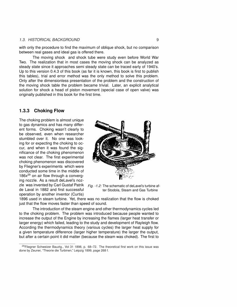
1.3. HISTORICAL BACKGROUND 9
with only the procedure to find the maximum of oblique shock, but no comparisonbetween real gases and ideal gas is offered there.
The moving shock and shock tube were study even before World WarTwo. The realization that in most cases the moving shock can be analyzed assteady state since it approaches semi steady state can be traced early of 1940’s.Up to this version 0.4.3 of this book (as far it is known, this book is first to publishthis tables), trial and error method was the only method to solve this problem.Only after the dimensionless presentation of the problem and the construction ofthe moving shock table the problem became trivial. Later, an explicit analyticalsolution for shock a head of piston movement (special case of open valve) wasoriginally published in this book for the first time.
1.3.3 Choking Flow
Fig. -1.2: The schematic of deLavel’s turbine af-ter Stodola, Steam and Gas Turbine
The choking problem is almost uniqueto gas dynamics and has many differ-ent forms. Choking wasn’t clearly tobe observed, even when researcherstumbled over it. No one was look-ing for or expecting the choking to oc-cur, and when it was found the sig-nificance of the choking phenomenonwas not clear. The first experimentalchoking phenomenon was discoveredby Fliegner’s experiments which wereconducted some time in the middle of186x29 on air flow through a converg-ing nozzle. As a result deLavel’s noz-zle was invented by Carl Gustaf Patrikde Laval in 1882 and first successfuloperation by another inventor (Curtis)1896 used in steam turbine. Yet, there was no realization that the flow is chokedjust that the flow moves faster than speed of sound.
The introduction of the steam engine and other thermodynamics cycles ledto the choking problem. The problem was introduced because people wanted toincrease the output of the Engine by increasing the flames (larger heat transfer orlarger energy) which failed, leading to the study and development of Rayleigh flow.According the thermodynamics theory (various cycles) the larger heat supply fora given temperature difference (larger higher temperature) the larger the output,but after a certain point it did matter (because the steam was choked). The first to
29Fliegner Schweizer Bauztg., Vol 31 1898, p. 68–72. The theoretical first work on this issue wasdone by Zeuner, “Theorie die Turbinen,” Leipzig 1899, page 268 f.

10 CHAPTER 1. INTRODUCTION
discover (try to explain) the choking phenomenon was Rayleigh30.
After the introduction of the deLavel’s converging–diverging nozzle theo-retical work was started by Zeuner31. Later continue by Prandtl’s group32 start-ing 1904. In 1908 Meyer has extend this work to make two dimensional calcula-tions33. Experimental work by Parenty34 and others measured the pressure alongthe converging-diverging nozzle.
It was commonly believed35 that the choking occurs only at M = 1. Thefirst one to analyzed that choking occurs at 1/
√k for isothermal flow was Shapiro
(195x). It is so strange that a giant like Shapiro did not realize his model on isother-mal contradict his conclusion from his own famous paper. Later Romer at el ex-tended it to isothermal variable area flow (1955). In this book, this author adaptsE.R.G. Ecert’s idea of dimensionless parameters control which determines wherethe reality lay between the two extremes. Recently this concept was proposed (notexplicitly) by Dutton and Converdill (1997)36. Namely, in many cases the reality issomewhere between the adiabatic and the isothermal flow. The actual results willbe determined by the modified Eckert number to which model they are closer.
30Rayleigh was the first to develop the model that bears his name. It is likely that others had noticedthat flow is choked, but did not produce any model or conduct successful experimental work.
31Zeuner, “Theorie der Turbinen, Leipzig 1899 page 268 f.32Some of the publications were not named after Prandtl but rather by his students like Meyer,
Theodor. In the literature appeared reference to article by Lorenz in the Physik Zeitshr., as if in 1904.Perhaps, there are also other works that this author did not come crossed.
33Meyer, Th., Uber zweidimensionals Bewegungsvordange eines Gases, Dissertation 1907, er-schienen in den Mitteilungen uber Forsch.-Arb. Ing.-Wes. heft 62, Berlin 1908.
34Parenty, Comptes R. Paris, Vol. 113, 116, 119; Ann. Chim. Phys. Vol. 8. 8 1896, Vol 12, 1897.35The personal experience of this undersigned shows that even instructors of Gas Dynamics are not
aware that the chocking occurs at different Mach number and depends on the model.36These researchers demonstrate results between two extremes and actually proposed this idea.
However, that the presentation here suggests that topic should be presented case between two ex-tremes.

1.3. HISTORICAL BACKGROUND 11
Fig. -1.3: The measured pressure in a nozzle takenfrom Stodola 1927 Steam and Gas Turbines
Nozzle Flow
The first “wind tunnel” was nota tunnel but a rotating arm at-tached at the center. At theend of the arm was the ob-ject that was under observationand study. The arm’s circularmotion could reach a velocityabove the speed of sound at itsend. Yet, in 1904 the Wrightbrothers demonstrated that re-sults from the wind tunnel andspinning arm are different, dueto the circular motion. As aresult, the spinning arm wasno longer used in testing. Be-tween the turn of the centuryand 1947-48, when the first su-personic wind tunnel was built,several models that explained choking at the throat have been built.
A different reason to study the converging-diverging nozzle was the Venturi me-ter which was used in measuring the flow rate of gases. Bendemann 37 carriedexperiments to study the accuracy of these flow meters and he measured and re-found that the flow reaches a critical value (pressure ratio of 0.545) that createsthe maximum flow rate.
There are two main models or extremes that describe the flow in the nozzle:isothermal and adiabatic.
37Bendemann Mitteil uber Forschungsarbeiten, Berlin, 1907, No. 37.

12 CHAPTER 1. INTRODUCTION
Nozzle flow
Fig. -1.4: Flow rate as a function of the back pressure takenafter Stodola 1927 Steam and Gas Turbines
Romer et al38 analyzed theisothermal flow in a nozzle.It is remarkable that chok-ing was found as 1/
√k as
opposed to one (1). In gen-eral when the model is as-sumed to be isothermal thechoking occurs at 1/
√k.
The concept that the chok-ing point can move from thethroat introduced by39 a re-searcher unknown to thisauthor. It is very interestingthat the isothermal nozzlewas proposed by Romerat el 1955 (who was be-hind the adviser or the stu-dent?). These researcherswere the first ones to real-ized that choking can occurs at different Mach number (1/
√k other then the
isothermal pipe.
Rayleigh Flow
Rayleigh was probably40, the first to suggest a model for frictionless flow with aconstant heat transfer. Rayleigh’s work was during the time when it was debatableas to whether there are two forms of energies (mechanical, thermal), even thoughWatt and others found and proved that they are the same. Therefore, Rayleighlooked at flow without mechanical energy transfer (friction) but only thermal energytransfer. In Rayleigh flow, the material reaches choking point due to heat transfer,hence term “thermally choked” is used; no additional flow can occur.
Fanno Flow
The most important model in compressible flow was suggested by Gino Fanno inhis Master’s thesis (1904). The model bears his name. Yet, according to Dr. Rudolf
39Romer, I Carl Jr., and Ali Bulent Cambel, “Analysis of Isothermal Variable Area Flow,” Aircraft Eng.vol. 27 no 322, p. 398 December 1955.
39This undersign didn’t find the actual trace to the source of proposing this effect. However, someastronomy books showing this effect in a dimensional form without mentioning the original researcher.In dimensionless form, this phenomenon produces a dimensionless number similar to Ozer numberand therefor the name Ozer number adapted in this book.
40As most of the history research has shown, there is also a possibility that someone found it earlier.For example, Simeon–Denis Poisson was the first one to realize the shock wave possibility.

1.3. HISTORICAL BACKGROUND 13
Mumenthaler from UTH University, no copy of the thesis can be found in the orig-inal University and perhaps only in the personal custody of the Fanno family41.Fanno attributes the main pressure reduction to friction. Thus, flow that is domi-nantly adiabatic could be simplified and analyzed. The friction factor is the maincomponent in the analysis as Darcy f42 had already proposed in 1845. The arrivalof the Moody diagram, which built on Hunter Rouse’s (194x) work made Darcy–Weisbach’s equation universally useful. Without the existence of the friction factordata, the Fanno model wasn’t able to produce a prediction useful for the indus-try. Additionally an understating of the supersonic branch of the flow was unknown(The idea of shock in tube was not raised at that time.). Shapiro organized all thematerial in a coherent way and made this model useful.
MetaDid Fanno realize that the flow is choked? It appears at least in Stodola’sbook that choking was understood in 1927 and even earlier. The chokingwas assumed only to be in the subsonic flow. But because the actual Fanno’sthesis is not available, the question cannot be answered yet. When wasGas Dynamics (compressible flow) as a separate class started? Did theexplanation for the combination of diverging-converging nuzzle with tube forFanno flow first appeared in Shapiro’s book?
Meta EndIsothermal Flow
The earliest reference to isothermal flow was found in Shapiro’s Book. The modelsuggests that the choking occurs at 1/
√k and it appears that Shapiro was the first
one to realize this difference compared to the other models. In reality, the flow ischoked somewhere between 1/
√k to one for cases that are between Fanno (adi-
abatic) and isothermal flow. This fact was evident in industrial applications wherethe expectation of the choking is at Mach one, but can be explained by choking ata lower Mach number. No experimental evidence, known by the undersigned, wasever produced to verify this finding.
1.3.4 External flow
When the flow over an external body is about .8 Mach or more the flow mustbe considered to be a compressible flow. However at a Mach number above 0.8(relative of velocity of the body to upstream velocity) a local Mach number (localvelocity) can reach M = 1. At that stage, a shock wave occurs which increasesthe resistance. The Navier-Stokes equations which describe the flow (or even
41This material is very important and someone should find it and make it available to researchers.42Fanning f based radius is only one quarter of the Darcy f which is based on diameter
14 CHAPTER 1. INTRODUCTION
Euler equations) were considered unsolvable during the mid 18xx because of thehigh complexity. This problem led to two consequences. Theoreticians tried tosimplify the equations and arrive at approximate solutions representing specificcases. Examples of such work are Hermann von Helmholtz’s concept of vortexfilaments (1858), Lanchester’s concept of circulatory flow (1894), and the Kutta-Joukowski circulation theory of lift (1906). Practitioners like the Wright brothersrelied upon experimentation to figure out what theory could not yet tell them.Ludwig Prandtl in 1904 explained the two most important causes of drag by intro-ducing the boundary layer theory. Prandtl’s boundary layer theory allowed varioussimplifications of the Navier-Stokes equations. Prandtl worked on calculating theeffect of induced drag on lift. He introduced the lifting line theory, which was pub-lished in 1918-1919 and enabled accurate calculations of induced drag and itseffect on lift43.During World War I, Prandtl created his thin–airfoil theory that enabled the calcula-tion of lift for thin, cambered airfoils. He later contributed to the Prandtl-Glauert rulefor subsonic airflow that describes the compressibility effects of air at high speeds.Prandtl’s student, Von Karman reduced the equations for supersonic flow into asingle equation.After the First World War aviation became important and in the 1920s a push ofresearch focused on what was called the compressibility problem. Airplanes couldnot yet fly fast, but the propellers (which are also airfoils) did exceed the speed ofsound, especially at the propeller tips, thus exhibiting inefficiency. Frank Caldwelland Elisha Fales demonstrated in 1918 that at a critical speed (later renamed thecritical Mach number) airfoils suffered dramatic increases in drag and decreasesin lift. Later, Briggs and Dryden showed that the problem was related to the shockwave. Meanwhile in Germany, one of Prandtl’s assistants, J. Ackeret, simplifiedthe shock equations so that they became easy to use. After World War Two, theresearch had continued and some technical solutions were found. Some of thesolutions lead to tedious calculations which lead to the creation of ComputationalFluid Dynamics (CFD). Today these methods of perturbations and asymptotic arehardly used in wing calculations44. That is the “dinosaur45” reason that even todaysome instructors are teaching mostly the perturbations and asymptotic methods inGas Dynamics classes.More information on external flow can be found in , John D. Anderson’s Book “His-tory of Aerodynamics and Its Impact on Flying Machines,” Cambridge UniversityPress, 1997
43The English call this theory the Lanchester-Prandtl theory. This is because the English AstronomerFrederick Lanchester published the foundation for Prandtl’s theory in his 1907 book Aerodynamics.However, Prandtl claimed that he was not aware of Lanchester’s model when he had begun his workin 1911. This claim seems reasonable in the light that Prandtl was not ware of earlier works when henamed erroneously the conditions for the shock wave. See for the full story in the shock section.
44This undersigned is aware of only one case that these methods were really used to calculations ofwing.
45It is like teaching using slide ruler in today school. By the way, slide rule is sold for about 7.5$ onthe net. Yet, there is no reason to teach it in a regular school.

1.3. HISTORICAL BACKGROUND 15
1.3.5 Filling and Evacuating Gaseous Chambers
It is remarkable that there were so few contributions made in the area of a fillingor evacuation gaseous chamber. The earlier work dealing with this issue was byGiffen, 1940, and was republished by Owczarek, J. A., the model and solution tothe nozzle attached to chamber issue in his book “Fundamentals of Gas Dynam-ics.”46. He also extended the model to include the unchoked case. Later severalresearchers mostly from the University in Illinois extended this work to isothermalnozzle (choked and unchoked).
The simplest model of nozzle, is not sufficient in many cases and a connection bya tube (rather just nozzle or orifice) is more appropriated. Since World War II con-siderable works have been carried out in this area but with very little progress47. In1993 the first reasonable models for forced volume were published by the under-signed. Later, that model was extended by several research groups, The analyti-cal solution for forced volume and the “balloon” problem (airbag’s problem) modelwere published first in this book (version 0.35) in 2005. The classification of fill-ing or evacuating the chamber as external control and internal control (mostly bypressure) was described in version 0.3 of this book by this author.
1.3.6 Biographies of Major Figures
In this section a short summary of major figures that influenced the field of gasdynamics is present. There are many figures that should be included and a biasedselection was required. Much information can be obtained from other resources,such as the Internet. In this section there is no originality and none should beexpected.
46International Textbook Co., Scranton, Pennsylvania, 1964.47In fact, the emergence of the CFD gave the illusion that there are solutions at hand, not realizing
that garbage in is garbage out, i.e., the model has to be based on scientific principles and not detachedfrom reality. As anecdotal story explaining the lack of progress, in die casting conference there wasa discussion and presentation on which turbulence model is suitable for a complete still liquid. Other“strange” models can be found in the undersigned’s book “Fundamentals of Die Casting Design.

16 CHAPTER 1. INTRODUCTION
Galileo Galilei
Fig. -1.5: Portrait of Galileo Galilei
Galileo was born in Pisa, Italy on Febru-ary 15, 1564 to musician VincenzoGalilei and Giulia degli Ammannati. Theoldest of six children, Galileo movedwith his family in early 1570 to Florence.Galileo started his studying at the Uni-versity of Pisa in 1581. He then becamea professor of mathematics at the Uni-versity of Padua in 1592. During thetime after his study, he made numerousdiscoveries such as that of the pendu-lum clock, (1602). Galileo also provedthat objects fell with the same velocityregardless of their size.
Galileo had a relationship with Marina Gamba (they never married) who lived andworked in his house in Padua, where she bore him three children. However, thisrelationship did not last and Marina married Giovanni Bartoluzzi and Galileo’s son,Vincenzio, joined him in Florence (1613).
Galileo invented many mechanical devices such as the pump and the telescope(1609). His telescopes helped him make many astronomic observations whichproved the Copernican system. Galileo’s observations got him into trouble withthe Catholic Church, however, because of his noble ancestry, the church was notharsh with him. Galileo was convicted after publishing his book Dialogue, and hewas put under house arrest for the remainder of his life. Galileo died in 1642 in hishome outside of Florence.

1.3. HISTORICAL BACKGROUND 17
Ernest Mach (1838-1916)
Fig. -1.6: Photo of Ernest Mach
Ernst Mach was born in 1838 inChrlice (now part of Brno), whenCzechia was still a part of theAustro–Hungary empire. Johann,Mach’s father, was a high schoolteacher who taught Ernst at homeuntil he was 14, when he stud-ied in Kromeriz Gymnasium, be-fore he entered the university of Vi-enna were he studies mathematics,physics and philosophy. He grad-uated from Vienna in 1860. ThereMach wrote his thesis ”On ElectricalDischarge and Induction.” Mach wasinterested also in physiology of sen-sory perception.At first he received a professorship position at Graz in mathematics (1864) andwas then offered a position as a professor of surgery at the university of Salzburg,but he declined. He then turned to physics, and in 1867 he received a position inthe Technical University in Prague48 where he taught experimental physics for thenext 28 years.Mach was also a great thinker/philosopher and influenced the theory of relativitydealing with frame of reference. In 1863, Ernest Mach (1836 - 1916) publishedDie Machanik in which he formalized this argument. Later, Einstein was greatlyinfluenced by it, and in 1918, he named it Mach’s Principle. This was one of theprimary sources of inspiration for Einstein’s theory of General Relativity.
Fig. -1.7: The Photo of the bullet in a supersonic flow thatMach made. Note it was not taken in a wind tunnel
Mach’s revolutionary exper-iment demonstrated the ex-istence of the shock waveas shown in Figure 1.7.It is amazing that Machwas able to photographthe phenomenon using thespinning arm technique (nowind tunnel was availableat that time and most def-initely nothing that couldtake a photo at supersonicspeeds. His experimentsrequired exact timing. He was not able to attach the camera to the arm and utilizethe remote control (not existent at that time). Mach’s shadowgraph technique and
48It is interesting to point out that Prague provided us two of the top influential researchers[:] E. Machand E.R.G. Eckert.

18 CHAPTER 1. INTRODUCTION
a related method called Schlieren Photography are still used today.Yet, Mach’s contributions to supersonic flow were not limited to experimental meth-ods alone. Mach understood the basic characteristics of external supersonic flowwhere the most important variable affecting the flow is the ratio of the speed of theflow49 (U) relative to the speed of sound (c). Mach was the first to note the transi-tion that occurs when the ratio U/c goes from being less than 1 to greater than 1.The name Mach Number (M) was coined by J. Ackeret (Prandtl’s student) in 1932in honor of Mach.
John William Strutt (Lord Rayleigh)
Fig. -1.8: Photo of Lord Rayleigh
A researcher with a wide interest, started stud-ies in compressible flow mostly from a math-ematical approach. At that time there wasn’tthe realization that the flow could be choked. Itseems that Rayleigh was the first who realizedthat flow with chemical reactions (heat transfer)can be choked.Lord Rayleigh was a British physicist born nearMaldon, Essex, on November 12, 1842. In 1861he entered Trinity College at Cambridge, wherehe commenced reading mathematics. His ex-ceptional abilities soon enabled him to overtakehis colleagues. He graduated in the Mathe-matical Tripos in 1865 as Senior Wrangler andSmith’s Prizeman. In 1866 he obtained a fellow-ship at Trinity which he held until 1871, the yearof his marriage. He served for six years as thepresident of the government committee on ex-plosives, and from 1896 to 1919 he acted as Scientific Adviser to Trinity House.He was Lord Lieutenant of Essex from 1892 to 1901.Lord Rayleigh’s first research was mainly mathematical, concerning optics and vi-brating systems, but his later work ranged over almost the whole field of physics,covering sound, wave theory, color vision, electrodynamics, electromagnetism,light scattering, flow of liquids, hydrodynamics, density of gases, viscosity, capillar-ity, elasticity, and photography. Rayleigh’s later work was concentrated on electricand magnetic problems. Rayleigh was considered to be an excellent instructor. HisTheory of Sound was published in two volumes during 1877-1878, and his otherextensive studies are reported in his Scientific Papers, six volumes issued during1889-1920. Rayleigh was also a contributer to the Encyclopedia Britannica. Hepublished 446 papers which, reprinted in his collected works, clearly show his ca-pacity for understanding everything just a little more deeply than anyone else. He
49Mach dealt with only air, but it is reasonable to assume that he understood that this ratio was appliedto other gases.

1.3. HISTORICAL BACKGROUND 19
intervened in debates of the House of Lords only on rare occasions, never allowingpolitics to interfere with science. Lord Rayleigh, a Chancellor of Cambridge Uni-versity, was a Justice of the Peace and the recipient of honorary science and lawdegrees. He was a Fellow of the Royal Society (1873) and served as Secretaryfrom 1885 to 1896, and as President from 1905 to 1908. He received the NobelPrize in 1904. Lord Rayleigh died on June 30, 1919, at Witham, Essex.
In 1871 he married Evelyn, sister of the future prime minister, the Earl of Balfour(of the famous Balfour declaration of the Jewish state). They had three sons, theeldest of whom was to become a professor of physics at the Imperial College ofScience and Technology, London.
As a successor to James Clerk Maxwell, he was head of the Cavendish Laboratoryat Cambridge from 1879-1884, and in 1887 became Professor of Natural Philos-ophy at the Royal Institute of Great Britain. Rayleigh died on June 30, 1919 atWitham, Essex.
William John Macquorn Rankine
Fig. -1.9: Portrait of Rankine
William John Macquorn Rankine (July 2,1820 - December 24, 1872) was a Scottishengineer and physicist. He was a foundingcontributor to the science of thermodynam-ics (Rankine Cycle). Rankine developed atheory of the steam engine. His steam en-gine manuals were used for many decades.Rankine was well rounded interested besidethe energy field he was also interested incivil engineering, strength of materials, andnaval engineering in which he was involvedin applying scientific principles to buildingships.Rankine was born in Edinburgh to BritishArmy lieutenant David Rankine and BarbaraGrahame, Rankine. Rankine never married, and his only brother and parents diedbefore him.

20 CHAPTER 1. INTRODUCTION
Gino Girolamo Fanno
Fig. -1.10: The photo of Gino Fanno ap-proximately in 1950
Fanno a Jewish Engineer was born onNovember 18, 1888. He studied in a tech-nical institute in Venice and graduated withvery high grades as a mechanical engi-neer. Fanno was not as lucky as hisbrother, who was able to get into academia.Faced with anti–semitism, Fanno left Italy forZurich, Switzerland in 1900 to attend gradu-ate school for his master’s degree. In thisnew place he was able to pose as a Ro-man Catholic, even though for short timehe went to live in a Jewish home, IsaakBaruch Weil’s family. As were many Jewsat that time, Fanno was fluent in several lan-guages including Italian, English, German,and French. He likely had a good knowl-edge of Yiddish and possibly some Hebrew.Consequently, he did not have a problem studying in a different language. In July1904 he received his diploma (master). When one of Professor Stodola’s assis-tants attended military service this temporary position was offered to Fanno. “Whydidn’t a talented guy like Fanno keep or obtain a position in academia after he pub-lished his model?” The answer is tied to the fact that somehow rumors about hisroots began to surface. Additionally, the fact that his model was not a “smashing50
success” did not help.
Later Fanno had to go back to Italy to find a job in industry. Fanno turned out to bea good engineer and he later obtained a management position. He married, andlike his brother, Marco, was childless. He obtained a Ph.D. from Regian IstitutoSuperiore d’Ingegneria di Genova. However, on February 1939 Fanno was de-graded (denounced) and he lost his Ph.D. (is this the first case in history) becausehis of his Jewish nationality51. During the War (WWII), he had to be under housearrest to avoid being sent to the “vacation camps.” To further camouflage himself,Fanno converted to Catholicism. Apparently, Fanno had a cache of old Italian cur-rency (which was apparently still highly acceptable) which helped him and his wifesurvive the war. After the war, Fanno was only able to work in agriculture and agri-cultural engineering. Fanno passed way in 1960 without world recognition for hismodel.Fanno’s older brother, mentioned earlier Marco Fanno is a famous economist wholater developed fundamentals of the supply and demand theory.
50Missing data about friction factor51In some places, the ridicules claims that Jews persecuted only because their religion. Clearly,
Fanno was not part of the Jewish religion (see his picture) only his nationality was Jewish.

1.3. HISTORICAL BACKGROUND 21
Ludwig Prandtl
Fig. -1.11: Photo of Prandtl
Perhaps Prandtl’s greatest achievementwas his ability to produce so many greatscientists. It is mind boggling to look atthe long list of those who were his stu-dents and colleagues. There is no onewho educated as many great scientistsas Prandtl. Prandtl changed the field offluid mechanics and is called the mod-ern father of fluid mechanics because ofhis introduction of boundary layer, tur-bulence mixing theories etc.Ludwig Prandtl was born in Freising,Bavaria, in 1874. His father was a pro-fessor of engineering and his mothersuffered from a lengthy illness. As a re-sult, the young Ludwig spent more timewith his father which made him inter-ested in his father’s physics and ma-chinery books. This upbringing fosteredthe young Prandtl’s interest in scienceand experimentation.Prandtl started his studies at the age of 20 in Munich, Germany and he graduatedat the age of 26 with a Ph.D. Interestingly, his Ph.D. was focused on solid mechan-ics. His interest changed when, in his first job, he was required to design factoryequipment that involved problems related to the field of fluid mechanics (a suctiondevice). Later he sought and found a job as a professor of mechanics at a tech-nical school in Hannover, Germany (1901). During this time Prandtl developed hisboundary layer theory and studied supersonic fluid flows through nozzles. In 1904,he presented the revolutionary paper “Flussigkeitsbewegung Bei Sehr Kleiner Rei-bung” (Fluid Flow in Very Little Friction), the paper which describes his boundarylayer theory.His 1904 paper raised Prandtl’s prestige. He became the director of the Institute forTechnical Physics at the University of Gottingen. He developed the Prandtl-Glauertrule for subsonic airflow. Prandtl, with his student Theodor Meyer, developed thefirst theory for calculating the properties of shock and expansion waves in super-sonic flow in 1908 (two chapters in this book). As a byproduct they produced thetheory for oblique shock. In 1925 Prandtl became the director of the Kaiser Wil-helm Institute for Flow Investigation at Gottingen. By the 1930s, he was knownworldwide as the leader in the science of fluid dynamics. Prandtl also contributedto research in many areas, such as meteorology and structural mechanics.Ludwig Prandtl worked at Gottingen until his death on August 15, 1953. His workand achievements in fluid dynamics resulted in equations that simplified under-standing, and many are still used today. Therefore many referred to him as the

22 CHAPTER 1. INTRODUCTION
father of modern fluid mechanics. Ludwig Prandtl died in Gottingen, Germany onAugust 15th 1953.Prandtl’s other contributions include: the introduction of the Prandtl number in fluidmechanics, airfoils and wing theory (including theories of aerodynamic interfer-ence, wing-fuselage, wing-propeller, biplane, etc); fundamental studies in the windtunnel, high speed flow (correction formula for subsonic compressible flows), the-ory of turbulence. His name is linked to the following:
• Prandtl number (heat transfer problems)
• Prandtl-Glauert compressibility correction
• Prandtl’s boundary layer equation
• Prandtl’s lifting line theory
• Prandtl’s law of friction for smooth pipes
• Prandtl-Meyer expansion fans (supersonic flow)
• Prandtl’s Mixing Length Concept (theory of turbulence)
E.R.G. Eckert
Fig. -1.12: The photo of Ernst Rudolf GeorgeEckert with the author’s family
Eckert was born in 1904 in Prague,where he studied at the German Insti-tute of Technology. During World WarII, he developed methods for jet engineturbine blade cooling at a research lab-oratory in Prague. He emigrated to theUnited States after the war, and servedas a consultant to the U.S. Air Forceand the National Advisory Committeefor Aeronautics before coming to Min-nesota.Eckert developed the understanding ofheat dissipation in relation to kinetic en-ergy, especially in compressible flow.Hence, the dimensionless group hasbeen designated as the Eckert number, which is associated with the Mach number.Schlichting suggested this dimensionless group in honor of Eckert. In addition tobeing named to the National Academy of Engineering in 1970, He authored morethan 500 articles and received several medals for his contributions to science. Hisbook ”Introduction to the Transfer of Heat and Mass,” published in 1937, is stillconsidered a fundamental text in the field.Eckert was an excellent mentor to many researchers (including this author), andhe had a reputation for being warm and kindly. He was also a leading figure inbringing together engineering in the East and West during the Cold War years.

1.3. HISTORICAL BACKGROUND 23
Ascher Shapiro
MIT Professor Ascher Shapiro52, the Eckert equivalent for the compressible flow,was instrumental in using his two volume book “The Dynamics of Thermodynamicsof the Compressible Fluid Flow,” to transform the gas dynamics field to a coherenttext material for engineers. Furthermore, Shapiro’s knowledge of fluid mechanicsenabled him to “sew” the missing parts of the Fanno line with Moody’s diagramto create the most useful model in compressible flow. While Shapiro viewed gasdynamics mostly through aeronautic eyes, The undersigned believes that Shapirowas the first one to propose an isothermal flow model that is not part of the aero-nautic field. Therefore it is proposed to call this model Shapiro’s Flow.In his first 25 years Shapiro focused primarily on power production, high-speedflight, turbomachinery and propulsion by jet engines and rockets. Unfortunately forthe field of Gas Dynamics, Shapiro moved to the field of biomedical engineeringwhere he was able to pioneer new work. Shapiro was instrumental in the treatmentof blood clots, asthma, emphysema and glaucoma.Shapiro grew up in New York City and received his S.B. in 1938 and the Sc.D. (Itis M.I.T.’s equivalent of a Ph.D. degree) in 1946 in mechanical engineering fromMIT. He was assistant professor in 1943, three years before receiving his Sc.D.In 1965 he become the head of the Department of Mechanical Engineering until1974. Shapiro spent most of his active years at MIT. Ascher Shapiro passed wayin November 2004.
52Parts taken from Sasha Brown, MIT

24 CHAPTER 1. INTRODUCTION

CHAPTER 2
Review of Thermodynamics
In this chapter, a review of several definitions of common thermodynamics terms ispresented. This introduction is provided to bring the student back to current placewith the material.
2.1 Basic DefinitionsThe following basic definitions are common to thermodynamics and will be used inthis book.
WorkIn mechanics, the work was defined as
mechanical work =∫
F • d` =∫
PdV (2.1)
This definition can be expanded to include two issues. The first issue that must beaddressed, that work done on the surroundings by the system boundaries similarlyis positive. Two, there is a transfer of energy so that its effect can cause work. Itmust be noted that electrical current is a work while heat transfer isn’t.
SystemThis term will be used in this book and it is defined as a continuous (at least par-tially) fixed quantity of matter. The dimensions of this material can be changed. Inthis definition, it is assumed that the system speed is significantly lower than thatof the speed of light. So, the mass can be assumed constant even though the trueconservation law applied to the combination of mass energy (see Einstein’s law).In fact for almost all engineering purpose this law is reduced to two separate lawsof mass conservation and energy conservation.
25
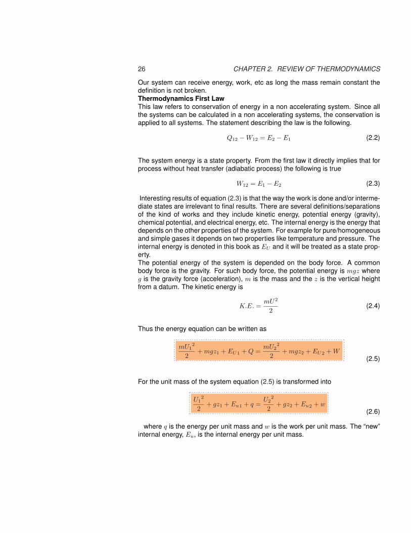
26 CHAPTER 2. REVIEW OF THERMODYNAMICS
Our system can receive energy, work, etc as long the mass remain constant thedefinition is not broken.Thermodynamics First LawThis law refers to conservation of energy in a non accelerating system. Since allthe systems can be calculated in a non accelerating systems, the conservation isapplied to all systems. The statement describing the law is the following.
Q12 −W12 = E2 − E1 (2.2)
The system energy is a state property. From the first law it directly implies that forprocess without heat transfer (adiabatic process) the following is true
W12 = E1 − E2 (2.3)
Interesting results of equation (2.3) is that the way the work is done and/or interme-diate states are irrelevant to final results. There are several definitions/separationsof the kind of works and they include kinetic energy, potential energy (gravity),chemical potential, and electrical energy, etc. The internal energy is the energy thatdepends on the other properties of the system. For example for pure/homogeneousand simple gases it depends on two properties like temperature and pressure. Theinternal energy is denoted in this book as EU and it will be treated as a state prop-erty.The potential energy of the system is depended on the body force. A commonbody force is the gravity. For such body force, the potential energy is mgz whereg is the gravity force (acceleration), m is the mass and the z is the vertical heightfrom a datum. The kinetic energy is
K.E. =mU2
2(2.4)
Thus the energy equation can be written as
mU12
2+ mgz1 + EU 1 + Q =
mU22
2+ mgz2 + EU 2 + W
(2.5)
For the unit mass of the system equation (2.5) is transformed into
U12
2+ gz1 + Eu1 + q =
U22
2+ gz2 + Eu2 + w
(2.6)
where q is the energy per unit mass and w is the work per unit mass. The “new”internal energy, Eu, is the internal energy per unit mass.

2.1. BASIC DEFINITIONS 27
Since the above equations are true between arbitrary points, choosing any point intime will make it correct. Thus differentiating the energy equation with respect totime yields the rate of change energy equation. The rate of change of the energytransfer is
DQ
Dt= Q (2.7)
In the same manner, the work change rate transfered through the boundaries ofthe system is
DW
Dt= W (2.8)
Since the system is with a fixed mass, the rate energy equation is
Q− W =D EU
Dt+ mU
DU
Dt+ m
D Bf z
Dt(2.9)
For the case were the body force, Bf , is constant with time like in the case ofgravity equation (2.9) reduced to
Q− W =D EU
Dt+ mU
DU
Dt+ mg
D z
Dt (2.10)
The time derivative operator, D/Dt is used instead of the common notation be-cause it referred to system property derivative.
Thermodynamics Second LawThere are several definitions of the second law. No matter which definition is usedto describe the second law it will end in a mathematical form. The most commonmathematical form is Clausius inequality which state that
∮δQ
T≥ 0 (2.11)
The integration symbol with the circle represent integral of cycle (therefor circle)in with system return to the same condition. If there is no lost, it is referred as areversible process and the inequality change to equality.
∮δQ
T= 0 (2.12)
The last integral can go though several states. These states are independent ofthe path the system goes through. Hence, the integral is independent of the path.This observation leads to the definition of entropy and designated as S and thederivative of entropy is
ds ≡(
δQ
T
)
rev(2.13)

28 CHAPTER 2. REVIEW OF THERMODYNAMICS
Performing integration between two states results in
S2 − S1 =∫ 2
1
(δQ
T
)
rev=
∫ 2
1
dS (2.14)
One of the conclusions that can be drawn from this analysis is for reversible andadiabatic process dS = 0. Thus, the process in which it is reversible and adiabatic,the entropy remains constant and referred to as isentropic process. It can be notedthat there is a possibility that a process can be irreversible and the right amount ofheat transfer to have zero change entropy change. Thus, the reverse conclusionthat zero change of entropy leads to reversible process, isn’t correct.For reversible process equation (2.12) can be written as
δQ = TdS (2.15)
and the work that the system is doing on the surroundings is
δW = PdV (2.16)
Substituting equations (2.15) (2.16) into (2.10) results in
TdS = dEU + PdV (2.17)
Even though the derivation of the above equations were done assuming that thereis no change of kinetic or potential energy, it still remail valid for all situations. Fur-thermore, it can be shown that it is valid for reversible and irreversible processes.Enthalpy
It is a common practice to define a new property, which is the combination of al-ready defined properties, the enthalpy of the system.
H = EU + PV (2.18)
The specific enthalpy is enthalpy per unit mass and denoted as, h.Or in a differential form as
dH = dEU + dP V + P dV (2.19)
Combining equations (2.18) the (2.17) yields
TdS = dH − V dP (2.20)
For isentropic process, equation (2.17) is reduced to dH = V dP . The equation(2.17) in mass unit is
Tds = du + Pdv = dh− dP
ρ(2.21)

2.1. BASIC DEFINITIONS 29
when the density enters through the relationship of ρ = 1/v.
Specific HeatsThe change of internal energy and enthalpy requires new definitions. The firstchange of the internal energy and it is defined as the following
Cv ≡(
∂Eu
∂T
)
(2.22)
And since the change of the enthalpy involve some kind of work is defined as
Cp ≡(
∂h
∂T
)
(2.23)
The ratio between the specific pressure heat and the specific volume heat is calledthe ratio of the specific heat and it is denoted as, k.
k ≡ Cp
Cv(2.24)
For solid, the ratio of the specific heats is almost 1 and therefore the differencebetween them is almost zero. Commonly the difference for solid is ignored andboth are assumed to be the same and therefore referred as C. This approximationless strong for liquid but not by that much and in most cases it applied to thecalculations. The ratio the specific heat of gases is larger than one.Equation of stateEquation of state is a relation between state variables. Normally the relationship oftemperature, pressure, and specific volume define the equation of state for gases.The simplest equation of state referred to as ideal gas. and it is defined as
P = ρRT (2.25)
Application of Avogadro’s law, that ”all gases at the same pressures and tempera-tures have the same number of molecules per unit of volume,” allows the calculationof a “universal gas constant.” This constant to match the standard units results in
R = 8.3145kj
kmol K(2.26)
Thus, the specific gas can be calculate as
R =R
M(2.27)

30 CHAPTER 2. REVIEW OF THERMODYNAMICS
Table -2.1: Properties of Various Ideal Gases [300K]
Gas ChemicalFormula
MolecularWeight R
[kj
KgK
]Cv
[kj
KgK
]CP
[kj
KgK
]k
Air - 28.970 0.28700 1.0035 0.7165 1.400Argon Ar 39.948 0.20813 0.5203 0.3122 1.400Butane C4H10 58.124 0.14304 1.7164 1.5734 1.091CarbonDioxide
CO2 44.01 0.18892 0.8418 0.6529 1.289
CarbonMonoxide
CO 28.01 0.29683 1.0413 0.7445 1.400
Ethane C2H6 30.07 0.27650 1.7662 1.4897 1.186Ethylene C2H4 28.054 0.29637 1.5482 1.2518 1.237Helium He 4.003 2.07703 5.1926 3.1156 1.667Hydrogen H2 2.016 4.12418 14.2091 10.0849 1.409Methane CH4 16.04 0.51835 2.2537 1.7354 1.299Neon Ne 20.183 0.41195 1.0299 0.6179 1.667
Nitrogen N2 28.013 0.29680 1.0416 0.7448 1.400Octane C8H18 114.230 0.07279 1.7113 1.6385 1.044Oxygen O2 31.999 0.25983 0.9216 0.6618 1.393Propane C3H8 44.097 0.18855 1.6794 1.4909 1.327Steam H2O 18.015 0.48152 1.8723 1.4108 1.327
The specific constants for select gas at 300K is provided in table 2.1.From equation (2.25) of state for perfect gas it follows
d(Pv) = RdT (2.28)
For perfect gas
dh = dEu + d(Pv) = dEu + d(RT ) = f(T ) (only) (2.29)
From the definition of enthalpy it follows that
d(Pv) = dh− dEu (2.30)
Utilizing equation (2.28) and subsisting into equation (2.30) and dividing by dT

2.1. BASIC DEFINITIONS 31
yields
Cp − Cv = R (2.31)
This relationship is valid only for ideal/perfect gases.The ratio of the specific heats can be expressed in several forms as
Cv =R
k − 1 (2.32)
Cp =k R
k − 1 (2.33)
The specific heat ratio, k value ranges from unity to about 1.667. These valuesdepend on the molecular degrees of freedom (more explanation can be obtainedin Van Wylen “F. of Classical thermodynamics.” The values of several gases canbe approximated as ideal gas and are provided in Table (2.1).The entropy for ideal gas can be simplified as the following
s2 − s1 =∫ 2
1
(dh
T− dP
ρT
)(2.34)
Using the identities developed so far one can find that
s2 − s1 =∫ 2
1
CpdT
T−
∫ 2
1
R dP
P= Cp ln
T2
T1−R ln
P2
P1(2.35)
Or using specific heat ratio equation (2.35) transformed into
s2 − s1
R=
k
k − 1ln
T2
T1− ln
P2
P1(2.36)
For isentropic process, ∆s = 0, the following is obtained
lnT2
T1= ln
(P2
P1
) k−1k
(2.37)
There are several famous identities that results from equation (2.37) as
T2
T1=
(P2
P1
) k−1k
=(
P2
P1
)k−1
(2.38)

32 CHAPTER 2. REVIEW OF THERMODYNAMICS
The ideal gas model is a simplified version of the real behavior of real gas. The realgas has a correction factor to account for the deviations from the ideal gas model.This correction factor referred as the compressibility factor and defined as
Z =P V
R T(2.39)

CHAPTER 3
Fundamentals of Basic FluidMechanics
3.1 IntroductionThis chapter is a review of the fundamentals that the student is expected to know.The basic principles are related to the basic conservation principle. Several termswill be reviewed such as stream lines. In addition the basic Bernoulli’s equationwill be derived for incompressible flow and later for compressible flow. Severalapplication of the fluid mechanics will demonstrated. This material is not coveredin the history chapter.
3.2 Fluid Properties
3.3 Control Volume
3.4 Reynold’s Transport TheoremFor simplification the discussion will be focused on one dimensional control volumeand it will be generalzed later. The flow through a stream tube is assumed to beone-dimensional so that there isn’t any flow except at the tube opening. At theinitial time the mass that was in the tube was m0. The mass after a very short timeof dt is dm. For simplicity, it is assumed the control volume is a fixed boundary.The flow on the right through the opening and on the left is assumed to enter thestream tube while the flow is assumed to leave the stream tube.
33

34 CHAPTER 3. FUNDAMENTALS OF BASIC FLUID MECHANICS
Supposed that the fluid has a property η
dNs
dt
)= lim
∆t→0
Ns(t0 + ∆t)−Ns(t0)∆t
(3.1)

CHAPTER 4
Speed of Sound
4.1 MotivationIn traditional compressible flow classes there is very little discussion about thespeed of sound outside the ideal gas. The author thinks that this approach hasmany shortcomings. In a recent consultation an engineer1 design a industrial sys-tem that contains converting diverging nozzle with filter to remove small particlesfrom air. The engineer was well aware of the calculation of the nozzle. Thus, theengineer was able to predict that was a chocking point. Yet, the engineer wasnot ware of the effect of particles on the speed of sound. Hence, the actual flowrate was only half of his prediction. As it will shown in this chapter, the particlescan, in some situations, reduces the speed of sound by almost as half. With the“new” knowledge from the consultation the calculations were within the range ofacceptable results.
The above situation is not unique in the industry. It should be expectedthat engineers know how to manage this situation of non pure substances (likeclean air). The fact that the engineer knows about the chocking is great but it is notenough for today’s sophisticated industry2. In this chapter an introductory discus-sion is given about different situations which can appear the industry in regards tospeed of sound.
4.2 Introduction1Aerospace engineer that alumni of University of Minnesota, Aerospace Department.2Pardon, but a joke is must in this situation. A cat is pursuing a mouse and the mouse escape and
hide in the hole. Suddenly, the mouse hear a barking dog and a cat yelling. The mouse go out toinvestigate, and cat is catching the mouse. The mouse ask the cat I thought I hear a dog. The cat reply,yes you right. My teacher was right, one language is not enough today.
35

36 CHAPTER 4. SPEED OF SOUND
velocity=dU
P+dP
ρ+dρ
sound wave
c
P
ρ
dU
Fig. -4.1: A very slow moving piston in a still gas
The people had recognized for sev-eral hundred years that sound isa variation of pressure. The earssense the variations by frequencyand magnitude which are trans-ferred to the brain which translatesto voice. Thus, it raises the ques-tion: what is the speed of thesmall disturbance travel in a “quiet”medium. This velocity is referred to as the speed of sound.
To answer this question consider a piston moving from the left to the rightat a relatively small velocity (see Figure 4.1). The information that the piston ismoving passes thorough a single “pressure pulse.” It is assumed that if the velocityof the piston is infinitesimally small, the pulse will be infinitesimally small. Thus,the pressure and density can be assumed to be continuous.
c-dU
P+dP
ρ+dρ
Control volume aroundthe sound wave
c
Pρ
Fig. -4.2: Stationary sound wave and gas movesrelative to the pulse.
In the control volume it isconvenient to look at a control vol-ume which is attached to a pressurepulse. Applying the mass balanceyields
ρc = (ρ + dρ)(c− dU) (4.1)
or when the higher term dUdρ isneglected yields
ρdU = cdρ =⇒ dU =cdρ
ρ(4.2)
From the energy equation (Bernoulli’s equation), assuming isentropic flow andneglecting the gravity results
(c− dU)2 − c2
2+
dP
ρ= 0 (4.3)
neglecting second term (dU2) yield
−cdU +dP
ρ= 0 (4.4)
Substituting the expression for dU from equation (4.2) into equation (4.4) yields
c2
(dρ
ρ
)=
dP
ρ=⇒ c2 =
dP
dρ(4.5)
An expression is needed to represent the right hand side of equation (4.5). Foran ideal gas, P is a function of two independent variables. Here, it is considered

4.3. SPEED OF SOUND IN IDEAL AND PERFECT GASES 37
that P = P (ρ, s) where s is the entropy. The full differential of the pressure can beexpressed as follows:
dP =∂P
∂ρ
∣∣∣∣s
dρ +∂P
∂s
∣∣∣∣ρ
ds (4.6)
In the derivations for the speed of sound it was assumed that the flow is isentropic,therefore it can be written
dP
dρ=
∂P
∂ρ
∣∣∣∣s
(4.7)
Note that the equation (4.5) can be obtained by utilizing the momentumequation instead of the energy equation.
Example 4.1:Demonstrate that equation (4.5) can be derived from the momentum equation.
SOLUTIONThe momentum equation written for the control volume shown in Figure (4.2) is
PF︷ ︸︸ ︷
(P + dP )− P =
Rcs
U(ρUdA)︷ ︸︸ ︷(ρ + dρ)(c− dU)2 − ρc2 (4.8)
Neglecting all the relative small terms results in
dP = (ρ + dρ)
(c2 −»»»:∼ 0
2cdU +»»»»»:∼ 0dU2
)− ρc2 (4.9)
dP = c2dρ (4.10)
This yields the same equation as (4.5).
4.3 Speed of sound in ideal and perfect gasesThe speed of sound can be obtained easily for the equation of state for an idealgas (also perfect gas as a sub set) because of a simple mathematical expression.The pressure for an ideal gas can be expressed as a simple function of density, ρ,and a function “molecular structure” or ratio of specific heats, k namely
P = constant× ρk (4.11)

38 CHAPTER 4. SPEED OF SOUND
and hence
c =
√dP
dρ= k × constant× ρk−1 = k ×
P︷ ︸︸ ︷constant× ρk
ρ
= k × P
ρ(4.12)
Remember that P/ρ is defined for an ideal gas as RT , and equation (4.12) can bewritten as
c =√
kRT (4.13)
Example 4.2:Calculate the speed of sound in water vapor at 20[bar] and 350◦C, (a) utilizes thesteam table (b) assuming ideal gas.
SOLUTIONThe solution can be estimated by using the data from steam table3
c ∼√
∆P
∆ρs=constant
(4.14)
At 20[bar] and 350◦C: s = 6.9563[
kJK kg
]ρ = 6.61376
[kgm3
]
At 18[bar] and 350◦C: s = 7.0100[
kJK kg
]ρ = 6.46956
[kgm3
]
At 18[bar] and 300◦C: s = 6.8226[
kJK kg
]ρ = 7.13216
[kgm3
]
After interpretation of the temperature:At 18[bar] and 335.7◦C: s ∼ 6.9563
[kJ
K kg
]ρ ∼ 6.94199
[kgm3
]
and substituting into the equation yields
c =
√2000000.32823
= 780.5[ m
sec
](4.15)
for ideal gas assumption (data taken from Van Wylen and Sontag, Classical Ther-modynamics, table A 8.)
c =√
kRT ∼√
1.327× 461× (350 + 273) ∼ 771.5[ m
sec
]
Note that a better approximation can be done with a steam table, and it3This data is taken form Van Wylen and Sontag “Fundamentals of Classical Thermodynamics” 2nd
edition
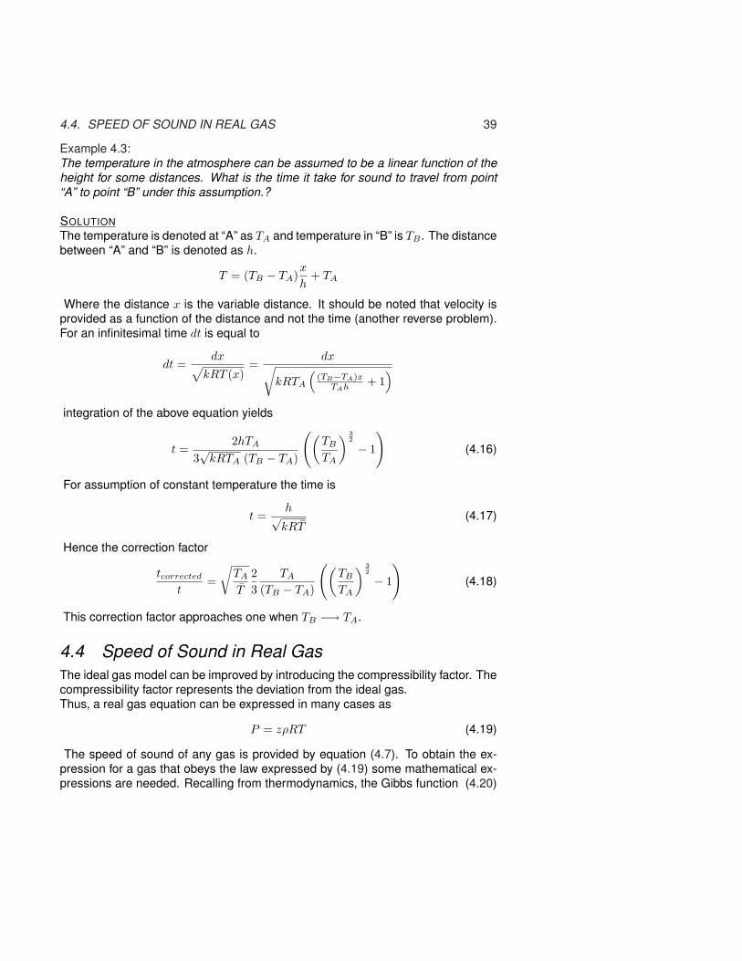
4.4. SPEED OF SOUND IN REAL GAS 39
Example 4.3:The temperature in the atmosphere can be assumed to be a linear function of theheight for some distances. What is the time it take for sound to travel from point“A” to point “B” under this assumption.?
SOLUTIONThe temperature is denoted at “A” as TA and temperature in “B” is TB . The distancebetween “A” and “B” is denoted as h.
T = (TB − TA)x
h+ TA
Where the distance x is the variable distance. It should be noted that velocity isprovided as a function of the distance and not the time (another reverse problem).For an infinitesimal time dt is equal to
dt =dx√
kRT (x)=
dx√kRTA
((TB−TA)x
TAh + 1)
integration of the above equation yields
t =2hTA
3√
kRTA (TB − TA)
((TB
TA
) 32
− 1
)(4.16)
For assumption of constant temperature the time is
t =h√kRT
(4.17)
Hence the correction factor
tcorrected
t=
√TA
T
23
TA
(TB − TA)
((TB
TA
) 32
− 1
)(4.18)
This correction factor approaches one when TB −→ TA.
4.4 Speed of Sound in Real GasThe ideal gas model can be improved by introducing the compressibility factor. Thecompressibility factor represents the deviation from the ideal gas.Thus, a real gas equation can be expressed in many cases as
P = zρRT (4.19)
The speed of sound of any gas is provided by equation (4.7). To obtain the ex-pression for a gas that obeys the law expressed by (4.19) some mathematical ex-pressions are needed. Recalling from thermodynamics, the Gibbs function (4.20)

40 CHAPTER 4. SPEED OF SOUND
Fig. -4.3: The Compressibility Chart
is used to obtain
Tds = dh− dP
ρ(4.20)
The definition of pressure specific heat for a pure substance is
Cp =(
∂h
∂T
)
P
= T
(∂s
∂T
)
P
(4.21)
The definition of volumetric specific heat for a pure substance is
Cv =(
∂u
∂T
)
ρ
= T
(∂s
∂T
)
ρ
(4.22)
From thermodynamics, it can be shown 4
dh = CpdT +[v − T
(∂v
∂T
)
P
](4.23)
4See Van Wylen p. 372 SI version, perhaps to insert the discussion here.

4.4. SPEED OF SOUND IN REAL GAS 41
The specific volumetric is the inverse of the density as v = zRT/P and thus
(∂v
∂T
)
P
=
(∂
(zRT
P
)
∂T
)
P
=RT
P
(∂z
∂T
)
P
+zR
P ½½
½½½>
1(∂T
∂T
)
P
(4.24)
Substituting the equation (4.24) into equation (4.23) results
dh = CpdT +
v − T
vz︷︸︸︷
RT
P
(∂z
∂T
)
P
+
vT︷︸︸︷
zR
P
dP (4.25)
Simplifying equation (4.25) to became
dh = CpdT −[Tv
z
(∂z
∂T
)
P
]dP = CpdT − T
z
(∂z
∂T
)
P
dP
ρ(4.26)
Utilizing Gibbs equation (4.20)
Tds =
dh︷ ︸︸ ︷CpdT − T
z
(∂z
∂T
)
P
dP
ρ−dP
ρ= CpdT − dP
ρ
[T
z
(∂z
∂T
)
P
+ 1]
=CpdT − dP
P
zRT︷︸︸︷P
ρ
[T
z
(∂z
∂T
)
P
+ 1]
(4.27)
Letting ds = 0 for isentropic process results in
dT
T=
dP
P
R
Cp
[z + T
(∂z
∂T
)
P
](4.28)
Equation (4.28) can be integrated by parts. However, it is more convenient toexpress dT/T in terms of Cv and dρ/ρ as follows
dT
T=
dρ
ρ
R
Cv
[z + T
(∂z
∂T
)
ρ
](4.29)
Equating the right hand side of equations (4.28) and (4.29) results in
dρ
ρ
R
Cv
[z + T
(∂z
∂T
)
ρ
]=
dP
P
R
Cp
[z + T
(∂z
∂T
)
P
](4.30)
Rearranging equation (4.30) yields
dρ
ρ=
dP
P
Cv
Cp
[z + T
(∂z∂T
)P
z + T(
∂z∂T
)ρ
](4.31)

42 CHAPTER 4. SPEED OF SOUND
If the terms in the braces are constant in the range under interest in this study,equation (4.31) can be integrated. For short hand writing convenience, n is definedas
n =
k︷︸︸︷Cp
Cv
(z + T
(∂z∂T
)ρ
z + T(
∂z∂T
)P
)(4.32)
Note that n approaches k when z → 1 and when z is constant. The integration ofequation (4.31) yields
(ρ1
ρ2
)n
=P1
P2(4.33)
Equation (4.33) is similar to equation (4.11). What is different in these derivationsis that a relationship between coefficient n and k was established. This relationship(4.33) isn’t new, and in–fact any thermodynamics book shows this relationship. Butthe definition of n in equation (4.32) provides a tool to estimate n. Now, the speedof sound for a real gas can be obtained in the same manner as for an ideal gas.
dP
dρ= nzRT
(4.34)
Example 4.4:Calculate the speed of sound of air at 30◦C and atmospheric pressure ∼ 1[bar].The specific heat for air is k = 1.407, n = 1.403, and z = 0.995.Make the calculation based on the ideal gas model and compare these calculationsto real gas model (compressibility factor). Assume that R = 287[j/kg/K].
SOLUTIONAccording to the ideal gas model the speed of sound should be
c =√
kRT =√
1.407× 287× 300 ∼ 348.1[m/sec]
For the real gas first coefficient n = 1.403 has
c =√
znRT =√
1.403× 0.995times287× 300 = 346.7[m/sec]
The correction factor for air under normal conditions (atmospheric conditions oreven increased pressure) is minimal on the speed of sound. However, a changein temperature can have a dramatical change in the speed of sound. For example,at relative moderate pressure but low temperature common in atmosphere, thecompressibility factor, z = 0.3 and n ∼ 1 which means that speed of sound is only√
0.31.4 about factor of (0.5) to calculated by ideal gas model.
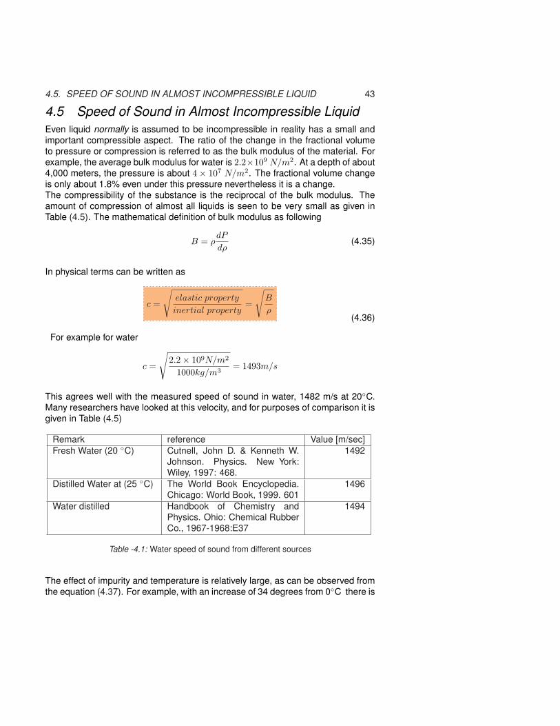
4.5. SPEED OF SOUND IN ALMOST INCOMPRESSIBLE LIQUID 43
4.5 Speed of Sound in Almost Incompressible LiquidEven liquid normally is assumed to be incompressible in reality has a small andimportant compressible aspect. The ratio of the change in the fractional volumeto pressure or compression is referred to as the bulk modulus of the material. Forexample, the average bulk modulus for water is 2.2×10⁹ N/m2. At a depth of about4,000 meters, the pressure is about 4 × 10⁷ N/m2. The fractional volume changeis only about 1.8% even under this pressure nevertheless it is a change.The compressibility of the substance is the reciprocal of the bulk modulus. Theamount of compression of almost all liquids is seen to be very small as given inTable (4.5). The mathematical definition of bulk modulus as following
B = ρdP
dρ(4.35)
In physical terms can be written as
c =
√elastic property
inertial property=
√B
ρ(4.36)
For example for water
c =
√2.2× 10⁹N/m2
1000kg/m3= 1493m/s
This agrees well with the measured speed of sound in water, 1482 m/s at 20◦C.Many researchers have looked at this velocity, and for purposes of comparison it isgiven in Table (4.5)
Remark reference Value [m/sec]Fresh Water (20 ◦C) Cutnell, John D. & Kenneth W.
Johnson. Physics. New York:Wiley, 1997: 468.
1492
Distilled Water at (25 ◦C) The World Book Encyclopedia.Chicago: World Book, 1999. 601
1496
Water distilled Handbook of Chemistry andPhysics. Ohio: Chemical RubberCo., 1967-1968:E37
1494
Table -4.1: Water speed of sound from different sources
The effect of impurity and temperature is relatively large, as can be observed fromthe equation (4.37). For example, with an increase of 34 degrees from 0◦C there is

44 CHAPTER 4. SPEED OF SOUND
an increase in the velocity from about 1430 m/sec to about 1546 [m/sec]. Accordingto Wilson5, the speed of sound in sea water depends on temperature, salinity, andhydrostatic pressure.Wilson’s empirical formula appears as follows:
c(S, T, P ) = c0 + cT + cS + cP + cSTP , (4.37)
where c0 = 1449.14[m/sec] is about clean/pure water, cT is a function temperature,and cS is a function salinity, cP is a function pressure, and cSTP is a correctionfactor between coupling of the different parameters.
material reference Value [m/sec]Glycerol 1904Sea water 25◦C 1533Mercury 1450Kerosene 1324Methyl alcohol 1143Carbon tetrachloride 926
Table -4.2: Liquids speed of sound, after Aldred, John, Manual of Sound Recording, Lon-don: Fountain Press, 1972
In summary, the speed of sound in liquids is about 3 to 5 relative to the speed ofsound in gases.
4.6 Speed of Sound in SolidsThe situation with solids is considerably more complicated, with different speedsin different directions, in different kinds of geometries, and differences betweentransverse and longitudinal waves. Nevertheless, the speed of sound in solids islarger than in liquids and definitely larger than in gases.Young’s Modulus for a representative value for the bulk modulus for steel is 160109 N /m2.Speed of sound in solid of steel, using a general tabulated value for the bulk mod-ulus, gives a sound speed for structural steel of
c =
√E
ρ=
√160× 109N/m2
7860Kg/m3= 4512m/s (4.38)
Compared to one tabulated value the example values for stainless steel lays be-tween the speed for longitudinal and transverse waves.
5 J. Acoust. Soc. Amer., 1960, vol.32, N 10, p. 1357. Wilson’s formula is accepted by the NationalOceanographic Data Center (NODC) USA for computer processing of hydrological information.

4.7. SOUND SPEED IN TWO PHASE MEDIUM 45
material reference Value [m/sec]Diamond 12000Pyrex glass 5640Steel longitudinal wave 5790Steel transverse shear 3100Steel longitudinal wave (extensional
wave)5000
Iron 5130Aluminum 5100Brass 4700Copper 3560Gold 3240Lucite 2680Lead 1322Rubber 1600
Table -4.3: Solids speed of sound, after Aldred, John, Manual of Sound Recording, Lon-don:Fountain Press, 1972
4.7 Sound Speed in Two Phase MediumThe gas flow in many industrial situations contains other particles. In actuality,there could be more than one speed of sound for two phase flow. Indeed there isdouble chocking phenomenon in two phase flow. However, for homogeneous andunder certain condition a single velocity can be considered. There can be severalmodels that approached this problem. For simplicity, it assumed that two materialsare homogeneously mixed. Topic for none homogeneous mixing are beyond thescope of this book. It further assumed that no heat and mass transfer occursbetween the particles. In that case, three extreme cases suggest themselves:the flow is mostly gas with drops of the other phase (liquid or solid), about equalparts of gas and the liquid phase, and liquid with some bubbles. The first case isanalyzed.The equation of state for the gas can be written as
Pa = ρaRTa (4.39)
The average density can be expressed as
1ρm
=ξ
ρa+
1− ξ
ρb(4.40)
where ξ = mb
m is the mass ratio of the materials.For small value of ξ equation (4.40) can be approximated as
ρ
ρa= 1 + m (4.41)

46 CHAPTER 4. SPEED OF SOUND
where m = mb
mais mass flow rate per gas flow rate.
The gas density can be replaced by equation (4.39) and substituted into equation(4.41)
P
ρ=
R
1 + mT (4.42)
A approximation of addition droplets of liquid or dust (solid) results in reduction ofR and yet approximate equation similar to ideal gas was obtained. It must noticedthat m = constant. If the droplets (or the solid particles) can be assumed to havethe same velocity as the gas with no heat transfer or fiction between the particlesisentropic relation can be assumed as
P
ρak
= constant (4.43)
Assuming that partial pressure of the particles is constant and applying the secondlaw for the mixture yields
0 =
droplets︷ ︸︸ ︷mC
dT
T+
gas︷ ︸︸ ︷Cp
dT
T−R
dP
P=
(Cp + mC)dT
T−R
dP
P(4.44)
Therefore, the mixture isentropic relationship can be expressed as
Pγ−1
γ
T= constant (4.45)
whereγ − 1
γ=
R
Cp + mC(4.46)
Recalling that R = Cp − Cv reduces equation (4.46) into
γ =Cp + mC
Cv + mC(4.47)
In a way the definition of γ was so chosen that effective specific pressure heatand effective specific volumetric heat are Cp+mC
1+m and Cv+mC1+m respectively. The
correction factors for the specific heat is not linear.Since the equations are the same as before hence the familiar equation for speedof sound can be applied as
c =√
γRmixT(4.48)
It can be noticed that Rmix and γ are smaller than similar variables in a puregas. Hence, this analysis results in lower speed of sound compared to pure gas.Generally, the velocity of mixtures with large gas component is smaller of the puregas. For example, the velocity of sound in slightly wed steam can be about onethird of the pure steam speed of sound.

4.7. SOUND SPEED IN TWO PHASE MEDIUM 47
MetaFor a mixture of two phases, speed of sound can be expressed as
c2 =∂P
∂ρ=
∂P [f(X)]∂ρ
(4.49)
where X is defined as
X =s− sf (PB)sfg(PB)
(4.50)
Meta End

48 CHAPTER 4. SPEED OF SOUND

CHAPTER 5
Isentropic Flow
distance, x
P
P0
PB = P0
M > 1
Supersonic
SubsonicM < 1
Fig. -5.1: Flow of a compressible substance(gas) through a converging–diverging nozzle.
In this chapter a discussion on a steadystate flow through a smooth and con-tinuous area flow rate is presented.A discussion about the flow througha converging–diverging nozzle is alsopart of this chapter. The isentropic flowmodels are important because of twomain reasons: One, it provides the infor-mation about the trends and importantparameters. Two, the correction factorscan be introduced later to account fordeviations from the ideal state.
5.1 Stagnation State forIdeal Gas Model5.1.1 General Relationship
It is assumed that the flow is one–dimensional. Figure (5.1) describes a gas flow through a converging–divergingnozzle. It has been found that a theoretical state known as the stagnation stateis very useful in simplifying the solution and treatment of the flow. The stagnationstate is a theoretical state in which the flow is brought into a complete motionlesscondition in isentropic process without other forces (e.g. gravity force). Severalproperties that can be represented by this theoretical process which include tem-perature, pressure, and density et cetera and denoted by the subscript “0.”
49

50 CHAPTER 5. ISENTROPIC FLOW
First, the stagnation temperature is calculated. The energy conservationcan be written as
h +U2
2= h0 (5.1)
Perfect gas is an ideal gas with a constant heat capacity, Cp. For perfect gasequation (5.1) is simplified into
CpT +U2
2= CpT0 (5.2)
Again it is common to denote T0 as the stagnation temperature. Recalling fromthermodynamic the relationship for perfect gas
R = Cp − Cv (5.3)
and denoting k ≡ Cp ÷Cv then the thermodynamics relationship obtains the form
Cp =kR
k − 1(5.4)
and where R is a specific constant. Dividing equation (5.2) by (CpT ) yields
1 +U2
2CpT=
T0
T(5.5)
Now, substituting c2 = kRT or T = c2/kR equation (5.5) changes into
1 +kRU2
2Cpc2=
T0
T(5.6)
By utilizing the definition of k by equation (2.24) and inserting it into equation (5.6)yields
1 +k − 1
2U2
c2=
T0
T(5.7)
It very useful to convert equation (5.6) into a dimensionless form and de-note Mach number as the ratio of velocity to speed of sound as
M ≡ U
c(5.8)
Inserting the definition of Mach number (5.8) into equation (5.7) reads
T0
T= 1 +
k − 12
M2
(5.9)

5.1. STAGNATION STATE FOR IDEAL GAS MODEL 51
velocity
T0
QA B
P0ρ0
T0
P0
ρ0
Fig. -5.2: Perfect gas flows through a tube
The usefulness of Mach num-ber and equation (5.9) can be demon-strated by this following simple example.In this example a gas flows through atube (see Figure 5.2) of any shape canbe expressed as a function of only thestagnation temperature as opposed tothe function of the temperatures and ve-locities.
The definition of the stagnation state provides the advantage of compactwriting. For example, writing the energy equation for the tube shown in Figure (5.2)can be reduced to
Q = Cp(T0B − T0A)m (5.10)
The ratio of stagnation pressure to the static pressure can be expressedas the function of the temperature ratio because of the isentropic relationship as
P0
P=
(T0
T
) kk−1
=(
1 +k − 1
2M2
) kk−1
(5.11)
In the same manner the relationship for the density ratio is
ρ0
ρ=
(T0
T
) 1k−1
=(
1 +k − 1
2M2
) 1k−1
(5.12)
A new useful definition is introduced for the case when M = 1 and denoted bysuperscript “∗.” The special case of ratio of the star values to stagnation values aredependent only on the heat ratio as the following:
T ∗
T0=
c∗2
c02
=2
k + 1(5.13)
P ∗
P0=
(2
k + 1
) kk−1
(5.14)
ρ∗
ρ0=
(2
k + 1
) 1k−1
(5.15)

52 CHAPTER 5. ISENTROPIC FLOW
0 1 2 3 4 5 6 7 8 9Mach number
0
0.1
0.2
0.3
0.4
0.5
0.6
0.7
0.8
0.9
1
P/P0
ρ/ρ0T/T
0
Static Properties As A Function of Mach Number
Mon Jun 5 17:39:34 2006
Fig. -5.3: The stagnation properties as a function of the Mach number, k = 1.4
5.1.2 Relationships for Small Mach Number
Even with today’s computers a simplified method can reduce the tedious work in-volved in computational work. In particular, the trends can be examined with an-alytical methods. It further will be used in the book to examine trends in derivedmodels. It can be noticed that the Mach number involved in the above equationsis in a square power. Hence, if an acceptable error is of about %1 then M < 0.1provides the desired range. Further, if a higher power is used, much smaller errorresults. First it can be noticed that the ratio of temperature to stagnation tempera-ture, T
T0is provided in power series. Expanding of the equations according to the
binomial expansion of
(1 + x)n = 1 + nx +n(n− 1)x2
2!+
n(n− 1)(n− 2)x3
3!+ · · · (5.16)
will result in the same fashion
P0
P= 1 +
(k − 1)M2
4+
kM4
8+
2(2− k)M6
48· · · (5.17)

5.2. ISENTROPIC CONVERGING-DIVERGING FLOW IN CROSS SECTION 53
ρ0
ρ= 1 +
(k − 1)M2
4+
kM4
8+
2(2− k)M6
48· · · (5.18)
The pressure difference normalized by the velocity (kinetic energy) as correctionfactor is
P0 − P12ρU2
= 1 +
compressibility correction︷ ︸︸ ︷M2
4+
(2− k)M4
24+ · · · (5.19)
From the above equation, it can be observed that the correction factor approacheszero when M −→ 0 and then equation (5.19) approaches the standard equationfor incompressible flow.
The definition of the star Mach is ratio of the velocity and star speed ofsound at M = 1.
M∗ =U
c∗=
√k + 1
2M
(1− k − 1
4M2 + · · ·
)(5.20)
P0 − P
P=
kM2
2
(1 +
M2
4+ · · ·
)(5.21)
ρ0 − ρ
ρ=
M2
2
(1− kM2
4+ · · ·
)(5.22)
The normalized mass rate becomes
m
A=
√kP0
2M2
RT0
(1 +
k − 14
M2 + · · ·)
(5.23)
The ratio of the area to star area is
A
A∗=
(2
k + 1
) k+12(k−1)
(1M
+k + 1
4M +
(3− k)(k + 1)32
M3 + · · ·)
(5.24)
5.2 Isentropic Converging-Diverging Flow in Cross Sec-tion

54 CHAPTER 5. ISENTROPIC FLOW
TρP
U
T+dTρ+dρP+dPU+dU
Fig. -5.4: Control volume inside a converging-diverging nozzle.
The important sub case in this chap-ter is the flow in a converging–divergingnozzle. The control volume is shownin Figure (5.4). There are two mod-els that assume variable area flow:First is isentropic and adiabatic model.Second is isentropic and isothermalmodel. Clearly, the stagnation tem-perature, T0, is constant through theadiabatic flow because there isn’t heattransfer. Therefore, the stagnation pressure is also constant through the flow be-cause the flow isentropic. Conversely, in mathematical terms, equation (5.9) andequation (5.11) are the same. If the right hand side is constant for one variable, itis constant for the other. In the same argument, the stagnation density is constantthrough the flow. Thus, knowing the Mach number or the temperature will provideall that is needed to find the other properties. The only properties that need to beconnected are the cross section area and the Mach number. Examination of therelation between properties can then be carried out.
5.2.1 The Properties in the Adiabatic Nozzle
When there is no external work and heat transfer, the energy equation, reads
dh + UdU = 0 (5.25)
Differentiation of continuity equation, ρAU = m = constant, and dividing by thecontinuity equation reads
dρ
ρ+
dA
A+
dU
U= 0 (5.26)
The thermodynamic relationship between the properties can be expressed as
Tds = dh− dP
ρ(5.27)
For isentropic process ds ≡ 0 and combining equations (5.25) with (5.27) yields
dP
ρ+ UdU = 0 (5.28)
Differentiation of the equation state (perfect gas), P = ρRT , and dividing theresults by the equation of state (ρRT ) yields
dP
P=
dρ
ρ+
dT
T(5.29)

5.2. ISENTROPIC CONVERGING-DIVERGING FLOW IN CROSS SECTION 55
Obtaining an expression for dU/U from the mass balance equation (5.26) andusing it in equation (5.28) reads
dP
ρ− U2
dUU︷ ︸︸ ︷[
dA
A+
dρ
ρ
]= 0 (5.30)
Rearranging equation (5.30) so that the density, ρ, can be replaced by the staticpressure, dP/ρ yields
dP
ρ= U2
(dA
A+
dρ
ρ
dP
dP
)= U2
dA
A+
1c2︷︸︸︷dρ
dP
dP
ρ
(5.31)
Recalling that dP/dρ = c2 and substitute the speed of sound into equation (5.31)to obtain
dP
ρ
[1−
(U
c
)2]
= U2 dA
A(5.32)
Or in a dimensionless form
dP
ρ
(1−M2
)= U2 dA
A(5.33)
Equation (5.33) is a differential equation for the pressure as a function of the crosssection area. It is convenient to rearrange equation (5.33) to obtain a variablesseparation form of
dP =ρU2
A
dA
1−M2(5.34)
The pressure Mach number relationship
Before going further in the mathematical derivation it is worth looking at the phys-ical meaning of equation (5.34). The term ρU2/A is always positive (because allthe three terms can be only positive). Now, it can be observed that dP can be pos-itive or negative depending on the dA and Mach number. The meaning of the signchange for the pressure differential is that the pressure can increase or decrease.It can be observed that the critical Mach number is one. If the Mach number islarger than one than dP has opposite sign of dA. If Mach number is smaller than
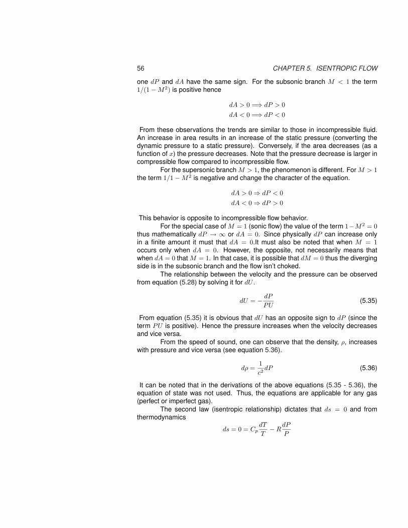
56 CHAPTER 5. ISENTROPIC FLOW
one dP and dA have the same sign. For the subsonic branch M < 1 the term1/(1−M2) is positive hence
dA > 0 =⇒ dP > 0dA < 0 =⇒ dP < 0
From these observations the trends are similar to those in incompressible fluid.An increase in area results in an increase of the static pressure (converting thedynamic pressure to a static pressure). Conversely, if the area decreases (as afunction of x) the pressure decreases. Note that the pressure decrease is larger incompressible flow compared to incompressible flow.
For the supersonic branch M > 1, the phenomenon is different. For M > 1the term 1/1−M2 is negative and change the character of the equation.
dA > 0 ⇒ dP < 0dA < 0 ⇒ dP > 0
This behavior is opposite to incompressible flow behavior.For the special case of M = 1 (sonic flow) the value of the term 1−M2 = 0
thus mathematically dP → ∞ or dA = 0. Since physically dP can increase onlyin a finite amount it must that dA = 0.It must also be noted that when M = 1occurs only when dA = 0. However, the opposite, not necessarily means thatwhen dA = 0 that M = 1. In that case, it is possible that dM = 0 thus the divergingside is in the subsonic branch and the flow isn’t choked.
The relationship between the velocity and the pressure can be observedfrom equation (5.28) by solving it for dU .
dU = − dP
PU(5.35)
From equation (5.35) it is obvious that dU has an opposite sign to dP (since theterm PU is positive). Hence the pressure increases when the velocity decreasesand vice versa.
From the speed of sound, one can observe that the density, ρ, increaseswith pressure and vice versa (see equation 5.36).
dρ =1c2
dP (5.36)
It can be noted that in the derivations of the above equations (5.35 - 5.36), theequation of state was not used. Thus, the equations are applicable for any gas(perfect or imperfect gas).
The second law (isentropic relationship) dictates that ds = 0 and fromthermodynamics
ds = 0 = CpdT
T−R
dP
P

5.2. ISENTROPIC CONVERGING-DIVERGING FLOW IN CROSS SECTION 57
and for perfect gas
dT
T=
k − 1k
dP
P(5.37)
Thus, the temperature varies according to the same way that pressure does.The relationship between the Mach number and the temperature can be
obtained by utilizing the fact that the process is assumed to be adiabatic dT0 = 0.Differentiation of equation (5.9), the relationship between the temperature and thestagnation temperature becomes
dT0 = 0 = dT
(1 +
k − 12
M2
)+ T (k − 1)MdM (5.38)
and simplifying equation (5.38) yields
dT
T= − (k − 1)MdM
1 + k−12 M2
(5.39)
Relationship Between the Mach Number and Cross Section Area
The equations used in the solution are energy (5.39), second law (5.37), state(5.29), mass (5.26)1. Note, equation (5.33) isn’t the solution but demonstration ofcertain properties on the pressure.
The relationship between temperature and the cross section area can beobtained by utilizing the relationship between the pressure and temperature (5.37)and the relationship of pressure and cross section area (5.33). First stage equation(5.39) is combined with equation (5.37) and becomes
(k − 1)k
dP
P= − (k − 1)MdM
1 + k−12 M2
(5.40)
Combining equation (5.40) with equation (5.33) yields
1k
ρU2
AdA
1−M2
P= − MdM
1 + k−12 M2
(5.41)
The following identify, ρU2 = kMP can be proved as
kM2P = k
M2
︷︸︸︷U2
c2
P︷︸︸︷ρRT = k
U2
kRT
P︷︸︸︷ρRT = ρU2 (5.42)
Using the identity in equation (5.42) changes equation (5.41) into
dA
A=
M2 − 1M
(1 + k−1
2 M2)dM (5.43)
1The momentum equation is not used normally in isentropic process, why?

58 CHAPTER 5. ISENTROPIC FLOW
M, Much nubmer
x
M, A
dAdx = 0 dMdx = 0A,
cross
sectio
n
Fig. -5.5: The relationship between the crosssection and the Mach number onthe subsonic branch
Equation (5.43) is very impor-tant because it relates the geometry(area) with the relative velocity (Machnumber). In equation (5.43), the factorsM
(1 + k−1
2 M2)
and A are positive re-gardless of the values of M or A. There-fore, the only factor that affects relation-ship between the cross area and theMach number is M2 − 1. For M < 1the Mach number is varied opposite tothe cross section area. In the case ofM > 1 the Mach number increases withthe cross section area and vice versa.The special case is when M = 1 whichrequires that dA = 0. This conditionimposes that internal2 flow has to passa converting–diverging device to obtainsupersonic velocity. This minimumarea is referred to as “throat.”
Again, the opposite conclusion that when dA = 0 implies that M = 1 isnot correct because possibility of dM = 0. In subsonic flow branch, from themathematical point of view: on one hand, a decrease of the cross section increasesthe velocity and the Mach number, on the other hand, an increase of the crosssection decreases the velocity and Mach number (see Figure (5.5)).
5.2.2 Isentropic Flow Examples
Example 5.1:Air is allowed to flow from a reservoir with temperature of 21◦C and with pressureof 5[MPa] through a tube. It was measured that air mass flow rate is 1[kg/sec]. Atsome point on the tube static pressure was measured to be 3[MPa]. Assume thatprocess is isentropic and neglect the velocity at the reservoir, calculate the Machnumber, velocity, and the cross section area at that point where the static pressurewas measured. Assume that the ratio of specific heat is k = Cp/Cv = 1.4.
SOLUTIONThe stagnation conditions at the reservoir will be maintained throughout the tubebecause the process is isentropic. Hence the stagnation temperature can be writ-ten T0 = constant and P0 = constant and both of them are known (the condition atthe reservoir). For the point where the static pressure is known, the Mach numbercan be calculated by utilizing the pressure ratio. With the known Mach number,
2This condition does not impose any restrictions for external flow. In external flow, an object can bemoved in arbitrary speed.

5.2. ISENTROPIC CONVERGING-DIVERGING FLOW IN CROSS SECTION 59
the temperature, and velocity can be calculated. Finally, the cross section can becalculated with all these information.In the point where the static pressure known
P =P
P0=
3[MPa]5[MPa]
= 0.6
From Table (5.2) or from Figure (5.3) or utilizing the enclosed program, Potto-GDC,or simply using the equations shows that
M TT0
ρρ0
AA?
PP0
A×PA∗×P0
FF∗
0.88639 0.86420 0.69428 1.0115 0.60000 0.60693 0.53105
With these values the static temperature and the density can be calculated.
T = 0.86420338× (273 + 21) = 254.076K
ρ =ρ
ρ0
ρ0︷︸︸︷P0
RT0= 0.69428839× 5× 106[Pa]
287.0[
JkgK
]× 294[K]
= 41.1416[
kg
m3
]
The velocity at that point is
U = M
c︷ ︸︸ ︷√kRT = 0.88638317×√1.4× 287× 294 = 304[m/sec]
The tube area can be obtained from the mass conservation as
A =m
ρU= 8.26× 10⁻⁵[m3]
For a circular tube the diameter is about 1[cm].
Example 5.2:The Mach number at point A on tube is measured to be M = 23 and the static pres-sure is 2[Bar]4. Downstream at point B the pressure was measured to be 1.5[Bar].Calculate the Mach number at point B under the isentropic flow assumption. Also,estimate the temperature at point B. Assume that the specific heat ratio k = 1.4and assume a perfect gas model.
4This pressure is about two atmospheres with temperature of 250[K]4Well, this question is for academic purposes, there is no known way for the author to directly mea-
sure the Mach number. The best approximation is by using inserted cone for supersonic flow andmeasure the oblique shock. Here it is subsonic and this technique is not suitable.

60 CHAPTER 5. ISENTROPIC FLOW
SOLUTIONWith the known Mach number at point A all the ratios of the static properties tototal (stagnation) properties can be calculated. Therefore, the stagnation pressureat point A is known and stagnation temperature can be calculated.At M = 2 (supersonic flow) the ratios are
M TT0
ρρ0
AA?
PP0
A×PA∗×P0
FF∗
2.0000 0.55556 0.23005 1.6875 0.12780 0.21567 0.59309
With this information the pressure at point B can be expressed as
PA
P0=
from the table5.2 @ M = 2︷︸︸︷
PB
P0×PA
PB= 0.12780453× 2.0
1.5= 0.17040604
The corresponding Mach number for this pressure ratio is 1.8137788 and TB =0.60315132 PB
P0= 0.17040879. The stagnation temperature can be “bypassed” to
calculate the temperature at point B
TB = TA ×
M=2︷︸︸︷T0
TA×
M=1.81..︷︸︸︷TB
T0= 250[K]× 1
0.55555556× 0.60315132 ' 271.42[K]
Example 5.3:Gas flows through a converging–diverging duct. At point “A” the cross section areais 50 [cm2] and the Mach number was measured to be 0.4. At point B in the ductthe cross section area is 40 [cm2]. Find the Mach number at point B. Assume thatthe flow is isentropic and the gas specific heat ratio is 1.4.
SOLUTIONTo obtain the Mach number at point B by finding the ratio of the area to the criticalarea. This relationship can be obtained by
AB
A∗ =AB
AA× AA
A∗=
4050×
from the Table 5.2︷ ︸︸ ︷1.59014 = 1.272112
With the value of AB
A∗ from the Table (5.2) or from Potto-GDC two solutions canbe obtained. The two possible solutions: the first supersonic M = 1.6265306 andsecond subsonic M = 0.53884934. Both solution are possible and acceptable. Thesupersonic branch solution is possible only if there where a transition at throatwhere M=1.
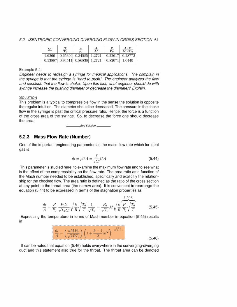
5.2. ISENTROPIC CONVERGING-DIVERGING FLOW IN CROSS SECTION 61
M TT0
ρρ0
AA?
PP0
A×PA∗×P0
1.6266 0.65396 0.34585 1.2721 0.22617 0.287720.53887 0.94511 0.86838 1.2721 0.82071 1.0440
Example 5.4:Engineer needs to redesign a syringe for medical applications. The complain inthe syringe is that the syringe is “hard to push.” The engineer analyzes the flowand conclude that the flow is choke. Upon this fact, what engineer should do withsyringe increase the pushing diameter or decrease the diameter? Explain.
SOLUTIONThis problem is a typical to compressible flow in the sense the solution is oppositethe regular intuition. The diameter should be decreased. The pressure in the chokeflow in the syringe is past the critical pressure ratio. Hence, the force is a functionof the cross area of the syringe. So, to decrease the force one should decreasethe area.
End Solution
5.2.3 Mass Flow Rate (Number)
One of the important engineering parameters is the mass flow rate which for idealgas is
m = ρUA =P
RTUA (5.44)
This parameter is studied here, to examine the maximum flow rate and to see whatis the effect of the compressibility on the flow rate. The area ratio as a function ofthe Mach number needed to be established, specifically and explicitly the relation-ship for the chocked flow. The area ratio is defined as the ratio of the cross sectionat any point to the throat area (the narrow area). It is convenient to rearrange theequation (5.44) to be expressed in terms of the stagnation properties as
m
A=
P
P0
P0U√kRT
√k
R
√T0
T
1√T0
=P0√T0
M
√k
R
f(M,k)︷ ︸︸ ︷P
P0
√T0
T(5.45)
Expressing the temperature in terms of Mach number in equation (5.45) resultsin
m
A=
(kMP0√kRT0
)(1 +
k − 12
M2
)− k+12(k−1)
(5.46)
It can be noted that equation (5.46) holds everywhere in the converging-divergingduct and this statement also true for the throat. The throat area can be denoted

62 CHAPTER 5. ISENTROPIC FLOW
as by A∗. It can be noticed that at the throat when the flow is chocked or in otherwords M = 1 and that the stagnation conditions (i.e. temperature, pressure) donot change. Hence equation (5.46) obtained the form
m
A∗=
(√kP0√RT0
) (1 +
k − 12
)− k+12(k−1)
(5.47)
Since the mass flow rate is constant in the duct, dividing equations (5.47) byequation (5.46) yields
A
A∗=
1M
(1 + k−1
2 M2
k+12
) k+12(k−1)
(5.48)
Equation (5.48) relates the Mach number at any point to the cross section arearatio.
The maximum flow rate can be expressed either by taking the derivative ofequation (5.47) in with respect to M and equating to zero. Carrying this calculationresults at M = 1.
(m
A∗
)
max
P0√T0
=
√k
R
(k + 1
2
)− k+12(k−1)
(5.49)
For specific heat ratio, k = 1.4(
m
A∗
)
max
P0√T0
∼ 0.68473√R
(5.50)
The maximum flow rate for air (R = 287j/kgK) becomes,
m√
T0
A∗P0= 0.040418 (5.51)
Equation (5.51) is known as Fliegner’s Formula on the name of one of the first en-gineers who observed experimentally the choking phenomenon. It can be noticedthat Fliengner’s equation can lead to definition of the Fliengner’s Number.
m√
T0
A∗P0=
m
c0︷ ︸︸ ︷√kRT0√
kRA∗P0
=
Fn︷ ︸︸ ︷mc0√RA∗P0
1√k
(5.52)
The definition of Fliengner’s number (Fn) is
Fn ≡ mc0√RA∗P0
(5.53)

5.2. ISENTROPIC CONVERGING-DIVERGING FLOW IN CROSS SECTION 63
Utilizing Fliengner’s number definition and substituting it into equation (5.47)results in
Fn = kM
(1 +
k − 12
M2
)− k+12(k−1)
(5.54)
and the maximum point for Fn at M = 1 is
Fn = k
(k + 1
2
)− k+12(k−1)
(5.55)
“Naughty Professor” Problems in Isentropic Flow
To explain the material better some instructors invented problems, which havemostly academic purpose, (see for example, Shapiro (problem 4.5)). While theseproblems have a limit applicability in reality, they have substantial academic valueand therefore presented here. The situation where the mass flow rate per areagiven with one of the stagnation properties and one of the static properties, e.g.P0 and T or T0 and P present difficulty for the calculations. The use of the regu-lar isentropic Table is not possible because there isn’t variable represent this kindproblems. For this kind of problems a new Table was constructed and presenthere5.The case of T0 and P
This case considered to be simplest case and will first presented here. Usingenergy equation (5.9) and substituting for Mach number M = m/Aρc results in
T0
T= 1 +
k − 12
(m
Aρc
)2
(5.56)
Rearranging equation (5.56) result in
T0ρ2 =
pR︷︸︸︷
Tρ ρ +
1/kR︷ ︸︸ ︷(T
c2
)k − 1
2
(m
A
)2
(5.57)
And further Rearranging equation (5.57) transformed it into
ρ2 =Pρ
T0R+
k − 12kRT0
(m
A
)2
(5.58)
5Since version 0.44 of this book.

64 CHAPTER 5. ISENTROPIC FLOW
Equation (5.58) is quadratic equation for density, ρ when all other variables areknown. It is convenient to change it into
ρ2 − Pρ
T0R− k − 1
2kRT0
(m
A
)2
= 0 (5.59)
The only physical solution is when the density is positive and thus the only solutionis
ρ =12
P
RT0+
√√√√√√
(P
RT0
)2
+ 2k − 1kRT0
(m
A
)2
︸ ︷︷ ︸↪→(M→0)→0
(5.60)
For almost incompressible flow the density is reduced and the familiar form ofperfect gas model is seen since stagnation temperature is approaching the statictemperature for very small Mach number (ρ = P
RT0). In other words, the terms
for the group over the under–brace approaches zero when the flow rate (Machnumber) is very small.
It is convenient to denote a new dimensionless density as
ρ =ρp
RT0
=ρRT0
P=
1T
(5.61)
With this new definition equation (5.60) is transformed into
ρ =12
1 +
√1 + 2
(k − 1)RT0
kP 2
(m
A
)2 (5.62)
The dimensionless density now is related to a dimensionless group that is a func-tion of Fn number and Mach number only! Thus, this dimensionless group is func-tion of Mach number only.
RT0
P 2
(m
A
)2
=1k
Fn2
︷ ︸︸ ︷c0
2
P02
(m
A∗
)2
A∗P0AP =f(M)︷ ︸︸ ︷(
A∗
A
)2 (P0
P
)2
(5.63)
Thus,
RT0
P 2
(m
A
)2
=Fn2
k
(A∗P0
AP
)2
(5.64)
Hence, the dimensionless density is
ρ =12
1 +
√1 + 2
(k − 1)Fn2
k2
(A∗P0
AP
)2 (5.65)

5.2. ISENTROPIC CONVERGING-DIVERGING FLOW IN CROSS SECTION 65
Again notice that the right hand side of equation (5.65) is only function of Machnumber (well, also the specific heat, k). And the values of AP
A∗P0were tabulated
in Table (5.2) and Fn is tabulated in the next Table (5.1). Thus, the problems isreduced to finding tabulated values.The case of P0 and T
A similar problem can be described for the case of stagnation pressure, P0,and static temperature, T .
First, it is shown that the dimensionless group is a function of Mach numberonly (well, again the specific heat ratio, k also).
RT
P02
(m
A
)2
=Fn2
k
(A∗P0
AP
)2 (T
T0
)(P0
P
)2
(5.66)
It can be noticed that
Fn2
k=
(T
T0
)(P0
P
)2
(5.67)
Thus equation (5.66) became
RT
P02
(m
A
)2
=(
A∗P0
AP
)2
(5.68)
The right hand side is tabulated in the “regular” isentropic Table such (5.2). Thisexample shows how a dimensional analysis is used to solve a problems withoutactually solving any equations. The actual solution of the equation is left as ex-ercise (this example under construction). What is the legitimacy of this method?The explanation simply based the previous experience in which for a given ratio ofarea or pressure ratio (etcetera) determines the Mach number. Based on the samearguments, if it was shown that a group of parameters depends only Mach numberthan the Mach is determined by this group.
The method of solution for given these parameters is by calculating the PAP0A∗
and then using the table to find the corresponding Mach number.The case of ρ0 and T or P
The last case sometimes referred to as the “naughty professor’s question” casedealt here is when the stagnation density given with the static temperature/pressure.First, the dimensionless approach is used later analytical method is discussed (un-der construction).
1Rρ0P
(m
A
)2
=
c02
︷ ︸︸ ︷kRT0
kRP0P0PP0
(m
A
)2
=c0
2
kRP02 P
P0
(m
A
)2
=Fn2
k
(P0
P
)(5.69)

66 CHAPTER 5. ISENTROPIC FLOW
The last case dealt here is of the stagnation density with static pressure and thefollowing is dimensionless group
1Rρ0
2T
(m
A
)2
=
c02
︷ ︸︸ ︷kRT0 T0
kRP02T
(m
A
)2
=c0
2T0
kRP02T
(m
A
)2
=Fn2
k
(T0
T
)(5.70)
It was hidden in the derivations/explanations of the above analysis didn’t explic-itly state under what conditions these analysis is correct. Unfortunately, not all theanalysis valid for the same conditions and is as the regular “isentropic” Table, (5.2).The heat/temperature part is valid for enough adiabatic condition while the pres-sure condition requires also isentropic process. All the above conditions/situationsrequire to have the perfect gas model as the equation of state. For example thefirst “naughty professor” question is sufficient that process is adiabatic only (T0, P ,mass flow rate per area.).
Table -5.1: Fliegner’s number and other parameters as a function of Mach number
M Fn ρ(
P0A∗
AP
)2RT0
P2
(mA
)2 1Rρ0P
(mA
)2 1Rρ0
2T
(mA
)2
0.00E+001.400E−061.000 0.0 0.0 0.0 0.00.050001 0.070106 1.000 0.00747 2.62E−05 0.00352 0.003510.10000 0.14084 1.000 0.029920 0.000424 0.014268 0.0141970.20000 0.28677 1.001 0.12039 0.00707 0.060404 0.0592120.21000 0.30185 1.001 0.13284 0.00865 0.067111 0.0656540.22000 0.31703 1.001 0.14592 0.010476 0.074254 0.0724870.23000 0.33233 1.002 0.15963 0.012593 0.081847 0.0797220.24000 0.34775 1.002 0.17397 0.015027 0.089910 0.0873720.25000 0.36329 1.003 0.18896 0.017813 0.098460 0.0954490.26000 0.37896 1.003 0.20458 0.020986 0.10752 0.103970.27000 0.39478 1.003 0.22085 0.024585 0.11710 0.112940.28000 0.41073 1.004 0.23777 0.028651 0.12724 0.122390.29000 0.42683 1.005 0.25535 0.033229 0.13796 0.132320.30000 0.44309 1.005 0.27358 0.038365 0.14927 0.142760.31000 0.45951 1.006 0.29247 0.044110 0.16121 0.153720.32000 0.47609 1.007 0.31203 0.050518 0.17381 0.165220.33000 0.49285 1.008 0.33226 0.057647 0.18709 0.177280.34000 0.50978 1.009 0.35316 0.065557 0.20109 0.189920.35000 0.52690 1.011 0.37474 0.074314 0.21584 0.203160.36000 0.54422 1.012 0.39701 0.083989 0.23137 0.217030.37000 0.56172 1.013 0.41997 0.094654 0.24773 0.231550.38000 0.57944 1.015 0.44363 0.10639 0.26495 0.246740.39000 0.59736 1.017 0.46798 0.11928 0.28307 0.262640.40000 0.61550 1.019 0.49305 0.13342 0.30214 0.27926

5.2. ISENTROPIC CONVERGING-DIVERGING FLOW IN CROSS SECTION 67
Table -5.1: Fliegner’s number and other parameters as function of Mach number (continue)
M Fn ρ(
P0A∗
AP
)2RT0
P2
(mA
)2 1Rρ0P
(mA
)2 1Rρ0
2T
(mA
)2
0.41000 0.63386 1.021 0.51882 0.14889 0.32220 0.296630.42000 0.65246 1.023 0.54531 0.16581 0.34330 0.314800.43000 0.67129 1.026 0.57253 0.18428 0.36550 0.333780.44000 0.69036 1.028 0.60047 0.20442 0.38884 0.353610.45000 0.70969 1.031 0.62915 0.22634 0.41338 0.374320.46000 0.72927 1.035 0.65857 0.25018 0.43919 0.395960.47000 0.74912 1.038 0.68875 0.27608 0.46633 0.418550.48000 0.76924 1.042 0.71967 0.30418 0.49485 0.442150.49000 0.78965 1.046 0.75136 0.33465 0.52485 0.466770.50000 0.81034 1.050 0.78382 0.36764 0.55637 0.492490.51000 0.83132 1.055 0.81706 0.40333 0.58952 0.519320.52000 0.85261 1.060 0.85107 0.44192 0.62436 0.547330.53000 0.87421 1.065 0.88588 0.48360 0.66098 0.576560.54000 0.89613 1.071 0.92149 0.52858 0.69948 0.607060.55000 0.91838 1.077 0.95791 0.57709 0.73995 0.638890.56000 0.94096 1.083 0.99514 0.62936 0.78250 0.672100.57000 0.96389 1.090 1.033 0.68565 0.82722 0.706750.58000 0.98717 1.097 1.072 0.74624 0.87424 0.742900.59000 1.011 1.105 1.112 0.81139 0.92366 0.780620.60000 1.035 1.113 1.152 0.88142 0.97562 0.819960.61000 1.059 1.122 1.194 0.95665 1.030 0.861010.62000 1.084 1.131 1.236 1.037 1.088 0.903820.63000 1.109 1.141 1.279 1.124 1.148 0.948480.64000 1.135 1.151 1.323 1.217 1.212 0.995070.65000 1.161 1.162 1.368 1.317 1.278 1.0440.66000 1.187 1.173 1.414 1.423 1.349 1.0940.67000 1.214 1.185 1.461 1.538 1.422 1.1470.68000 1.241 1.198 1.508 1.660 1.500 1.2020.69000 1.269 1.211 1.557 1.791 1.582 1.2600.70000 1.297 1.225 1.607 1.931 1.667 1.3200.71000 1.326 1.240 1.657 2.081 1.758 1.3820.72000 1.355 1.255 1.708 2.241 1.853 1.4480.73000 1.385 1.271 1.761 2.412 1.953 1.5160.74000 1.415 1.288 1.814 2.595 2.058 1.5870.75000 1.446 1.305 1.869 2.790 2.168 1.6610.76000 1.477 1.324 1.924 2.998 2.284 1.7380.77000 1.509 1.343 1.980 3.220 2.407 1.8190.78000 1.541 1.362 2.038 3.457 2.536 1.9030.79000 1.574 1.383 2.096 3.709 2.671 1.991

68 CHAPTER 5. ISENTROPIC FLOW
Table -5.1: Fliegner’s number and other parameters as function of Mach number (continue)
M Fn ρ(
P0A∗
AP
)2RT0
P2
(mA
)2 1Rρ0P
(mA
)2 1Rρ0
2T
(mA
)2
0.80000 1.607 1.405 2.156 3.979 2.813 2.0820.81000 1.642 1.427 2.216 4.266 2.963 2.1770.82000 1.676 1.450 2.278 4.571 3.121 2.2770.83000 1.712 1.474 2.340 4.897 3.287 2.3810.84000 1.747 1.500 2.404 5.244 3.462 2.4890.85000 1.784 1.526 2.469 5.613 3.646 2.6020.86000 1.821 1.553 2.535 6.006 3.840 2.7200.87000 1.859 1.581 2.602 6.424 4.043 2.8420.88000 1.898 1.610 2.670 6.869 4.258 2.9710.89000 1.937 1.640 2.740 7.342 4.484 3.1040.90000 1.977 1.671 2.810 7.846 4.721 3.2440.91000 2.018 1.703 2.882 8.381 4.972 3.3890.92000 2.059 1.736 2.955 8.949 5.235 3.5410.93000 2.101 1.771 3.029 9.554 5.513 3.6990.94000 2.144 1.806 3.105 10.20 5.805 3.8650.95000 2.188 1.843 3.181 10.88 6.112 4.0370.96000 2.233 1.881 3.259 11.60 6.436 4.2170.97000 2.278 1.920 3.338 12.37 6.777 4.4040.98000 2.324 1.961 3.419 13.19 7.136 4.6000.99000 2.371 2.003 3.500 14.06 7.515 4.8041.000 2.419 2.046 3.583 14.98 7.913 5.016
Example 5.5:A gas flows in the tube with mass flow rate of 0.1 [kg/sec] and tube cross sectionis 0.001[m2]. The temperature at Chamber supplying the pressure to tube is 27◦C.At some point the static pressure was measured to be 1.5[Bar]. Calculate for thatpoint the Mach number, the velocity, and the stagnation pressure. Assume that theprocess is isentropic, k = 1.3, R = 287[j/kgK].
SOLUTIONThe first thing that need to be done is to find the mass flow per area and it is
m
A= 0.1/0.001 = 100.0[kg/sec/m2]
It can be noticed that the total temperature is 300K and the static pressure is1.5[Bar]. The solution is based on section equations (5.60) through (5.65). It isfortunate that Potto-GDC exist and it can be just plug into it and it provide that
M TT0
ρρ0
AA?
PP0
A×PA∗×P0
FF∗
0.17124 0.99562 0.98548 3.4757 0.98116 3.4102 1.5392

5.2. ISENTROPIC CONVERGING-DIVERGING FLOW IN CROSS SECTION 69
The velocity can be calculated as
U = Mc =√
kRTM = 0.17×√1.3× 287× 300× ∼ 56.87[m/sec]
The stagnation pressure is
P0 =P
P/P0= 1.5/0.98116 = 1.5288[Bar]
Flow with pressure losses
The expression for the mass flow rate (5.46) is appropriate regardless the flow isisentropic or adiabatic. That expression was derived based on the theoretical totalpressure and temperature (Mach number) which does not based on the considera-tions whether the flow is isentropic or adiabatic. In the same manner the definitionof A∗ referred to the theoretical minimum area (”throat area”) if the flow continuesto flow in an isentropic manner. Clearly, in a case where the flow isn’t isentropic oradiabatic the total pressure and the total temperature will change (due to friction,and heat transfer). A constant flow rate requires that mA = mB . Denoting sub-script A for one point and subscript B for another point mass equation (5.47) canbe equated as
(kP0A
∗
RT0
)(1 +
k − 12
M2
)− k−12(k−1)
= constant (5.71)
From equation (5.71), it is clear that the function f(P0, T0, A∗) = constant. There
are two possible models that can be used to simplify the calculations. The firstmodel for neglected heat transfer (adiabatic) flow and in which the total temperatureremained constant (Fanno flow like). The second model which there is significantheat transfer but insignificant pressure loss (Rayleigh flow like).If the mass flow rate is constant at any point on the tube (no mass loss occur) then
m = A∗
√k
RT0
(2
k + 1
) k+1k−1
P0 (5.72)
For adiabatic flow, comparison of mass flow rate at point A and point B leads to
P0A∗|A = P0A
∗|B
;P0|AP0|B
=A∗|AA∗|B
(5.73)
And utilizing the equality of A∗ = A∗A A leads to
P0|AP0|B
=AA∗
∣∣MA
AA∗
∣∣MB
A|AA|B
(5.74)

70 CHAPTER 5. ISENTROPIC FLOW
For a flow with a constant stagnation pressure (frictionless flow) and non adiabaticflow reads
T0|AT0|B
=
[BA∗
∣∣MB
AA∗
∣∣MA
A|BA|A
]2
(5.75)
Example 5.6:At point A of the tube the pressure is 3[Bar], Mach number is 2.5, and the ductsection area is 0.01[m2]. Downstream at exit of tube, point B, the cross sectionarea is 0.015[m2] and Mach number is 1.5. Assume no mass lost and adiabaticsteady state flow, calculated the total pressure lost.
SOLUTIONBoth Mach numbers are known, thus the area ratios can be calculated. The to-tal pressure can be calculated because the Mach number and static pressure areknown. With these information, and utilizing equation (5.74) the stagnation pres-sure at point B can be obtained.
M TT0
ρρ0
AA?
PP0
A×PA∗×P0
FF∗
1.5000 0.68966 0.39498 1.1762 0.27240 0.32039 0.554012.5000 0.44444 0.13169 2.6367 0.05853 0.15432 0.62693
First, the stagnation at point A is obtained from Table (5.2) as
P0|A =P(P
P0
)
︸ ︷︷ ︸M=2.5
∣∣∣∣∣∣∣∣∣∣∣∣∣A
=3
0.058527663= 51.25781291[Bar]
by utilizing equation (5.74) provides
P0|B = 51.25781291× 1.17616712.6367187
× 0.010.015
≈ 15.243[Bar]
Hence
P0|A − P0|B = 51.257− 15.243 = 36.013[Bar]
Note that the large total pressure loss is much larger than the static pressure loss(Pressure point B the pressure is 0.27240307× 15.243 = 4.146[Bar]).
5.3 Isentropic Tables

5.3. ISENTROPIC TABLES 71
Table -5.2: Isentropic Table k = 1.4
M TT0
ρρ0
AA?
PP0
A×PA∗×P0
FF∗
0.000 1.00000 1.00000 5.8E+5 1.0000 5.8E + 5 2.4E+50.050 0.99950 0.99875 11.59 0.99825 11.57 4.8380.100 0.99800 0.99502 5.822 0.99303 5.781 2.4430.200 0.99206 0.98028 2.964 0.97250 2.882 1.2680.300 0.98232 0.95638 2.035 0.93947 1.912 0.896990.400 0.96899 0.92427 1.590 0.89561 1.424 0.726320.500 0.95238 0.88517 1.340 0.84302 1.130 0.635350.600 0.93284 0.84045 1.188 0.78400 0.93155 0.583770.700 0.91075 0.79158 1.094 0.72093 0.78896 0.554250.800 0.88652 0.73999 1.038 0.65602 0.68110 0.538070.900 0.86059 0.68704 1.009 0.59126 0.59650 0.530391.00 0.83333 0.63394 1.000 0.52828 0.52828 0.528281.100 0.80515 0.58170 1.008 0.46835 0.47207 0.529891.200 0.77640 0.53114 1.030 0.41238 0.42493 0.533991.300 0.74738 0.48290 1.066 0.36091 0.38484 0.539741.400 0.71839 0.43742 1.115 0.31424 0.35036 0.546551.500 0.68966 0.39498 1.176 0.27240 0.32039 0.554011.600 0.66138 0.35573 1.250 0.23527 0.29414 0.561821.700 0.63371 0.31969 1.338 0.20259 0.27099 0.569761.800 0.60680 0.28682 1.439 0.17404 0.25044 0.577681.900 0.58072 0.25699 1.555 0.14924 0.23211 0.585492.000 0.55556 0.23005 1.688 0.12780 0.21567 0.593092.500 0.44444 0.13169 2.637 0.058528 0.15432 0.626933.000 0.35714 0.076226 4.235 0.027224 0.11528 0.653263.500 0.28986 0.045233 6.790 0.013111 0.089018 0.673204.000 0.23810 0.027662 10.72 0.00659 0.070595 0.688304.500 0.19802 0.017449 16.56 0.00346 0.057227 0.699835.000 0.16667 0.011340 25.00 0.00189 0.047251 0.708765.500 0.14184 0.00758 36.87 0.00107 0.039628 0.715786.000 0.12195 0.00519 53.18 0.000633 0.033682 0.721366.500 0.10582 0.00364 75.13 0.000385 0.028962 0.725867.000 0.092593 0.00261 1.0E+2 0.000242 0.025156 0.729537.500 0.081633 0.00190 1.4E+2 0.000155 0.022046 0.732578.000 0.072464 0.00141 1.9E+2 0.000102 0.019473 0.735108.500 0.064725 0.00107 2.5E+2 6.90E−5 0.017321 0.737239.000 0.058140 0.000815 3.3E+2 4.74E−5 0.015504 0.739039.500 0.052493 0.000631 4.2E+2 3.31E−5 0.013957 0.74058
10.00 0.047619 0.000495 5.4E+2 2.36E−5 0.012628 0.74192
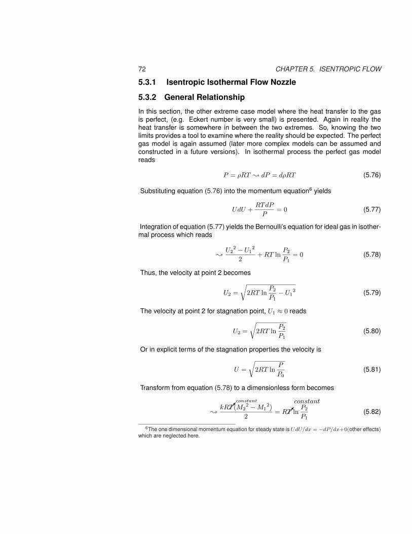
72 CHAPTER 5. ISENTROPIC FLOW
5.3.1 Isentropic Isothermal Flow Nozzle
5.3.2 General Relationship
In this section, the other extreme case model where the heat transfer to the gasis perfect, (e.g. Eckert number is very small) is presented. Again in reality theheat transfer is somewhere in between the two extremes. So, knowing the twolimits provides a tool to examine where the reality should be expected. The perfectgas model is again assumed (later more complex models can be assumed andconstructed in a future versions). In isothermal process the perfect gas modelreads
P = ρRT ; dP = dρRT (5.76)
Substituting equation (5.76) into the momentum equation6 yields
UdU +RTdP
P= 0 (5.77)
Integration of equation (5.77) yields the Bernoulli’s equation for ideal gas in isother-mal process which reads
;U2
2 − U12
2+ RT ln
P2
P1= 0 (5.78)
Thus, the velocity at point 2 becomes
U2 =√
2RT lnP2
P1− U1
2 (5.79)
The velocity at point 2 for stagnation point, U1 ≈ 0 reads
U2 =√
2RT lnP2
P1(5.80)
Or in explicit terms of the stagnation properties the velocity is
U =√
2RT lnP
P0(5.81)
Transform from equation (5.78) to a dimensionless form becomes
;kR¡¡µ
constant
T (M22 −M1
2)2
= R¡¡µ
constant
T lnP2
P1(5.82)
6The one dimensional momentum equation for steady state is UdU/dx = −dP/dx+0(other effects)which are neglected here.

5.3. ISENTROPIC TABLES 73
Simplifying equation (5.82) yields
;k(M2
2 −M12)
2= ln
P2
P1(5.83)
Or in terms of the pressure ratio equation (5.83) reads
P2
P1= e
k(M12−M2
2)2 =
(eM1
2
eM22
) k2
(5.84)
As oppose to the adiabatic case (T0 = constant) in the isothermal flow the stag-nation temperature ratio can be expressed
T01
T02
=¢¢¢1
T1
T2
(1 + k−1
2 M12)
(1 + k−1
2 M22) =
(1 + k−1
2 M12)
(1 + k−1
2 M22) (5.85)
Utilizing conservation of the mass AρM = constant to yield
A1
A2=
M2P2
M1P1(5.86)
Combining equation (5.86) and equation (5.84) yields
A2
A1=
M1
M2
(eM2
2
eM12
) k2
(5.87)
The change in the stagnation pressure can be expressed as
P02
P01
=P2
P1
(1 + k−1
2 M22
1 + k−12 M1
2
) kk−1
=
[eM1
2
eM12
] k2
(5.88)
The critical point, at this stage, is unknown (at what Mach number the nozzle ischoked is unknown) so there are two possibilities: the choking point or M = 1 tonormalize the equation. Here the critical point defined as the point where M = 1so results can be compared to the adiabatic case and denoted by star. Again ithas to emphasis that this critical point is not really related to physical critical pointbut it is arbitrary definition. The true critical point is when flow is choked and therelationship between two will be presented.The critical pressure ratio can be obtained from (5.84) to read
P
P ∗=
ρ
ρ∗= e
(1−M2)k2
(5.89)

74 CHAPTER 5. ISENTROPIC FLOW
Equation (5.87) is reduced to obtained the critical area ratio writes
A
A∗=
1M
e(1−M2)k
2
(5.90)
Similarly the stagnation temperature reads
T0
T0∗ =
2(1 + k−1
2 M12)
k + 1
kk−1
(5.91)
Finally, the critical stagnation pressure reads
P0
P0∗ = e
(1−M2)k2
(2
(1 + k−1
2 M12)
k + 1
) kk−1
(5.92)
The maximum value of stagnation pressure ratio is obtained when M = 0 at whichis
P0
P0∗
∣∣∣∣M=0
= e k2
(2
k + 1
) kk−1
(5.93)
For specific heat ratio of k = 1.4, this maximum value is about two. It can be notedthat the stagnation pressure is monotonically reduced during this process.Of course in isothermal process T = T ∗. All these equations are plotted in Figure(5.6). From the Figure 5.3 it can be observed that minimum of the curve A/A∗ isn’ton M = 1. The minimum of the curve is when area is minimum and at the pointwhere the flow is choked. It should be noted that the stagnation temperature is notconstant as in the adiabatic case and the critical point is the only one constant.The mathematical procedure to find the minimum is simply taking the derivativeand equating to zero as following
d(
AA∗
)
dM=
kM2ek(M2−1)
2 − ek(M2−1)
2
M2= 0 (5.94)
Equation (5.94) simplified to
kM2 − 1 = 0 ; M =1√k
(5.95)
It can be noticed that a similar results are obtained for adiabatic flow. The velocityat the throat of isothermal model is smaller by a factor of
√k. Thus, dividing the
critical adiabatic velocity by√
k results in
Uthroatmax =√
RT (5.96)
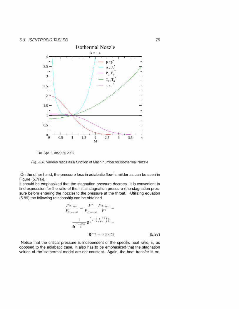
5.3. ISENTROPIC TABLES 75
0 0.5 1 1.5 2 2.5 3 3.5 4M
0
0.5
1
1.5
2
2.5
3
3.5
4
P / P*
A / A*
P0 /
P0
*
T0 /
T0
*
T / T*
Isothermal Nozzlek = 1 4
Tue Apr 5 10:20:36 2005
Fig. -5.6: Various ratios as a function of Mach number for isothermal Nozzle
On the other hand, the pressure loss in adiabatic flow is milder as can be seen inFigure (5.7(a)).It should be emphasized that the stagnation pressure decrees. It is convenient tofind expression for the ratio of the initial stagnation pressure (the stagnation pres-sure before entering the nozzle) to the pressure at the throat. Utilizing equation(5.89) the following relationship can be obtained
Pthroat
P0initial
=P ∗
P0initial
Pthroat
P ∗=
1
e(1−02)k
2
e„
1−“
1√k
”2«
k2 =
e− 12 = 0.60653 (5.97)
Notice that the critical pressure is independent of the specific heat ratio, k, asopposed to the adiabatic case. It also has to be emphasized that the stagnationvalues of the isothermal model are not constant. Again, the heat transfer is ex-
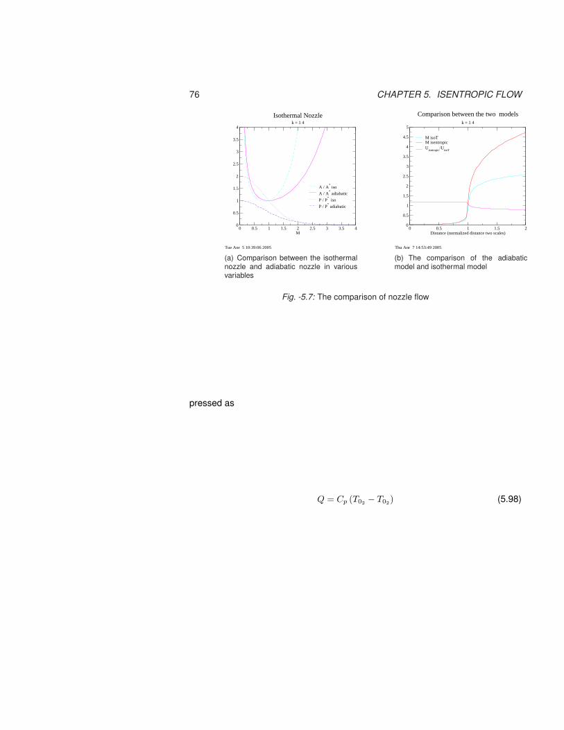
76 CHAPTER 5. ISENTROPIC FLOW
0 0.5 1 1.5 2 2.5 3 3.5 4M
0
0.5
1
1.5
2
2.5
3
3.5
4
A / A* iso
A / A* adiabatic
P / P*
iso
P / P* adiabatic
Isothermal Nozzlek = 1 4
Tue Apr 5 10:39:06 2005
(a) Comparison between the isothermalnozzle and adiabatic nozzle in variousvariables
0 0.5 1 1.5 2Distance (normalized distance two scales)
0
0.5
1
1.5
2
2.5
3
3.5
4
4.5
5
M isoTM isentropicU
isntropic/U
isoT
Comparison between the two models k = 1 4
Thu Apr 7 14:53:49 2005
(b) The comparison of the adiabaticmodel and isothermal model
Fig. -5.7: The comparison of nozzle flow
pressed as
Q = Cp (T02 − T02) (5.98)

5.3. ISENTROPIC TABLES 77
0 0.5 1 1.5 2Distance (normalized distance two scales)
0
0.2
0.4
0.6
0.8
1
P / P0 isentropic
T / T0 isentropic
P / P0 isothermal
T/T0 isothermal
Comparison between the two models k = 1 4
Fri Apr 8 15:11:44 2005
Fig. -5.8: Comparison of the pressure and temperaturedrop as a function of the normalized length(two scales)
For comparison betweenthe adiabatic model and theisothermal a simple profile ofnozzle area as a function ofthe distance is assumed. Thisprofile isn’t an ideal profilebut rather a simple samplejust to examine the differencebetween the two models so inan actual situation it can bebounded. To make sense andeliminate unnecessary detailsthe distance from the entranceto the throat is normalized (toone (1)). In the same fashionthe distance from the throat tothe exit is normalized (to one(1)) (it doesn’t mean that thesedistances are the same). In thiscomparison the entrance arearatio and the exit area ratio arethe same and equal to 20. The Mach number was computed for the two modelsand plotted in Figure (5.7(b)). In this comparison it has to be remembered thatcritical area for the two models are different by about 3% (for k = 1.4). As can beobserved from Figure (5.7(b)). The Mach number for the isentropic is larger forthe supersonic branch but the velocity is lower. The ratio of the velocities can beexpressed as
Us
UT=
Ms
√kRTs
MT
√kRTs
(5.99)
It can be noticed that temperature in the isothermal model is constant while tem-perature in the adiabatic model can be expressed as a function of the stagnationtemperature. The initial stagnation temperatures are almost the same and can becanceled out to obtain
Us
UT∼ Ms
MT
√1 + k−1
2 Ms2
(5.100)
By utilizing equation (5.100) the velocity ratio was obtained and is plotted in Figure(5.7(b)).Thus, using the isentropic model results in under prediction of the actual results forthe velocity in the supersonic branch. While, the isentropic for the subsonic branchwill be over prediction. The prediction of the Mach number are similarly shown inFigure (5.7(b)).

78 CHAPTER 5. ISENTROPIC FLOW
Two other ratios need to be examined: temperature and pressure. The initial stag-nation temperature is denoted as T0int. The temperature ratio of T/T0int can beobtained via the isentropic model as
T
T0int
=1
1 + k−12 M2
(5.101)
While the temperature ratio of the isothermal model is constant and equal to one(1). The pressure ratio for the isentropic model is
P
P0int
=1
(1 + k−1
2 M2) k−1
k
(5.102)
and for the isothermal process the stagnation pressure varies and has to be takeninto account as the following:
Pz
P0int
=P0∗
P0int
P0z
P0∗
isentropic︷︸︸︷Pz
P0z
(5.103)
where z is an arbitrary point on the nozzle. Using equations (5.88) and the isen-tropic relationship, the sought ratio is provided.Figure (5.8) shows that the range between the predicted temperatures of the twomodels is very large, while the range between the predicted pressure by the twomodels is relatively small. The meaning of this analysis is that transferred heataffects the temperature to a larger degree but the effect on the pressure is muchless significant.To demonstrate the relativity of the approach advocated in this book consider thefollowing example.
Example 5.7:Consider a diverging–converging nozzle made out of wood (low conductive mate-rial) with exit area equal entrance area. The throat area ratio to entrance area is1:4 respectively. The stagnation pressure is 5[Bar] and the stagnation temperatureis 27◦C. Assume that the back pressure is low enough to have supersonic flowwithout shock and k = 1.4. Calculate the velocity at the exit using the adiabaticmodel. If the nozzle was made from copper (a good heat conductor) a larger heattransfer occurs, should the velocity increase or decrease? What is the maximumpossible increase?
SOLUTIONThe first part of the question deals with the adiabatic model i.e. the conservationof the stagnation properties. Thus, with known area ratio and known stagnationPotto–GDC provides the following table:

5.4. THE IMPULSE FUNCTION 79
M TT0
ρρ0
AA?
PP0
A×PA∗×P0
0.14655 0.99572 0.98934 4.0000 0.98511 3.94052.9402 0.36644 0.08129 4.0000 0.02979 0.11915
With the known Mach number and temperature at the exit, the velocity can becalculated. The exit temperature is 0.36644×300 = 109.9K. The exit velocity, then,is
U = M√
kRT = 2.9402√
1.4× 287× 109.9 ∼ 617.93[m/sec]
Even for the isothermal model, the initial stagnation temperature is given as 300K.Using the area ratio in Figure (5.6) or using the Potto–GDC obtains the followingtable
M TT0
ρρ0
AA?
PP0
A×PA∗×P0
1.9910 1.4940 0.51183 4.0000 0.12556 0.50225
The exit Mach number is known and the initial temperature to the throat tempera-ture ratio can be calculated as the following:
T0ini
T0∗ =
11 + k−1
21k
=1
1 + k−1k
= 0.777777778
Thus the stagnation temperature at the exit is
T0ini
T0exit
= 1.4940/0.777777778 = 1.921
The exit stagnation temperature is 1.92 × 300 = 576.2K. The exit velocity can bedetermined by utilizing the following equation
Uexit = M√
kRT = 1.9910√
1.4× 287× 300.0 = 691.253[m/sec]
As was discussed before, the velocity in the copper nozzle will be larger than thevelocity in the wood nozzle. However, the maximum velocity cannot exceed the691.253[m/sec]
5.4 The Impulse Function5.4.1 Impulse in Isentropic Adiabatic Nozzle
One of the functions that is used in calculating the forces is the Impulse function.The Impulse function is denoted here as F , but in the literature some denote thisfunction as I. To explain the motivation for using this definition consider the calcu-lation of the net forces that acting on section shown in Figure (5.9). To calculatethe net forces acting in the x–direction the momentum equation has to be applied
Fnet = m(U2 − U1) + P2A2 − P1A1 (5.104)

80 CHAPTER 5. ISENTROPIC FLOW
The net force is denoted here as Fnet. The mass conservation also can be appliedto our control volume
m = ρ1A1U1 = ρ2A2U2 (5.105)
Combining equation (5.104) with equation (5.105) and by utilizing the identity inequation (5.42) results in
Fnet = kP2A2M22 − kP1A1M1
2 + P2A2 − P1A1 (5.106)
Rearranging equation (5.106) and dividing it by P0A∗ results in
Fnet
P0A∗=
f(M2)︷ ︸︸ ︷P2A2
P0A∗
f(M2)︷ ︸︸ ︷(1 + kM2
2)−
f(M1)︷ ︸︸ ︷P1A1
P0A∗
f(M1)︷ ︸︸ ︷(1 + kM1
2)
(5.107)
x-direction
Fig. -5.9: Schematic to explain the signifi-cances of the Impulse function
Examining equation (5.107) shows thatthe right hand side is only a function ofMach number and specific heat ratio, k.Hence, if the right hand side is only afunction of the Mach number and k thanthe left hand side must be function ofonly the same parameters, M and k.Defining a function that depends onlyon the Mach number creates the con-venience for calculating the net forcesacting on any device. Thus, defining the Impulse function as
F = PA(1 + kM2
2)
(5.108)
In the Impulse function when F (M = 1) is denoted as F ∗
F ∗ = P ∗A∗ (1 + k) (5.109)
The ratio of the Impulse function is defined as
F
F ∗=
P1A1
P ∗A∗
(1 + kM1
2)
(1 + k)=
1P ∗
P0︸︷︷︸( 2
k+1 )k
k−1
see function (5.107)︷ ︸︸ ︷P1A1
P0A∗(1 + kM1
2) 1
(1 + k)(5.110)
This ratio is different only in a coefficient from the ratio defined in equation (5.107)which makes the ratio a function of k and the Mach number. Hence, the net forceis
Fnet = P0A∗(1 + k)
(k + 1
2
) kk−1
(F2
F ∗− F1
F ∗
)(5.111)

5.4. THE IMPULSE FUNCTION 81
To demonstrate the usefulness of the this function consider a simple situation ofthe flow through a converging nozzle
Example 5.8:1
2m = 1[kg/sec]
A1 = 0.009m2
T0 = 400KA2 = 0.003m2
P2 = 50[Bar]
Fig. -5.10: Schematic of a flow of a compressible sub-stance (gas) thorough a converging nozzlefor example (5.8)
Consider a flow of gas into aconverging nozzle with a massflow rate of 1[kg/sec] and theentrance area is 0.009[m2] andthe exit area is 0.003[m2]. Thestagnation temperature is 400Kand the pressure at point 2 wasmeasured as 5[Bar] Calculatethe net force acting on the noz-zle and pressure at point 1.
SOLUTIONThe solution is obtained by getting the data for the Mach number. To obtained theMach number, the ratio of P1A1/A
∗P0 is needed to be calculated. To obtain thisratio the denominator is needed to be obtained. Utilizing Fliegner’s equation (5.51),provides the following
A∗P0 =m√
RT
0.058=
1.0×√400× 2870.058
∼ 70061.76[N ]
andA2P2
A∗P0=
500000× 0.00370061.76
∼ 2.1
M TT0
ρρ0
AA?
PP0
A×PA∗×P0
FF∗
0.27353 0.98526 0.96355 2.2121 0.94934 2.1000 0.96666
With the area ratio of AA? = 2.2121 the area ratio of at point 1 can be calculated.
A1
A?=
A2
A?
A1
A2= 2.2121× 0.009
0.003= 5.2227
And utilizing again Potto-GDC provides
M TT0
ρρ0
AA?
PP0
A×PA∗×P0
FF∗
0.11164 0.99751 0.99380 5.2227 0.99132 5.1774 2.1949
The pressure at point 1 is
P1 = P2P0
P2
P1
P0= 5.0times0.94934/0.99380 ∼ 4.776[Bar]

82 CHAPTER 5. ISENTROPIC FLOW
The net force is obtained by utilizing equation (5.111)
Fnet = P2A2P0A
∗
P2A2(1 + k)
(k + 1
2
) kk−1
(F2
F ∗− F1
F ∗
)
= 500000× 12.1
× 2.4× 1.23.5 × (2.1949− 0.96666) ∼ 614[kN ]
5.4.2 The Impulse Function in Isothermal Nozzle
Previously Impulse function was developed in the isentropic adiabatic flow. Thesame is done here for the isothermal nozzle flow model. As previously, the defi-nition of the Impulse function is reused. The ratio of the impulse function for twopoints on the nozzle is
F2
F1=
P2A2 + ρ2U22A2
P1A1 + ρ1U12A1
(5.112)
Utilizing the ideal gas model for density and some rearrangement results in
F2
F1=
P2A2
P1A1
1 + U22
RT
1 + U12
RT
(5.113)
Since U2/RT = kM2 and the ratio of equation (5.86) transformed equation into(5.113)
F2
F1=
M1
M2
1 + kM22
1 + kM12 (5.114)
At the star condition (M = 1) (not the minimum point) results in
F2
F ∗=
1M2
1 + kM22
1 + k (5.115)
5.5 Isothermal Table
Table -5.3: Isothermal Table
M T0
T0?
P0
P0?
AA?
PP?
A×PA∗×P0
FF∗
0.00 0.52828 1.064 5.0E + 5 2.014 1.0E+6 4.2E+5
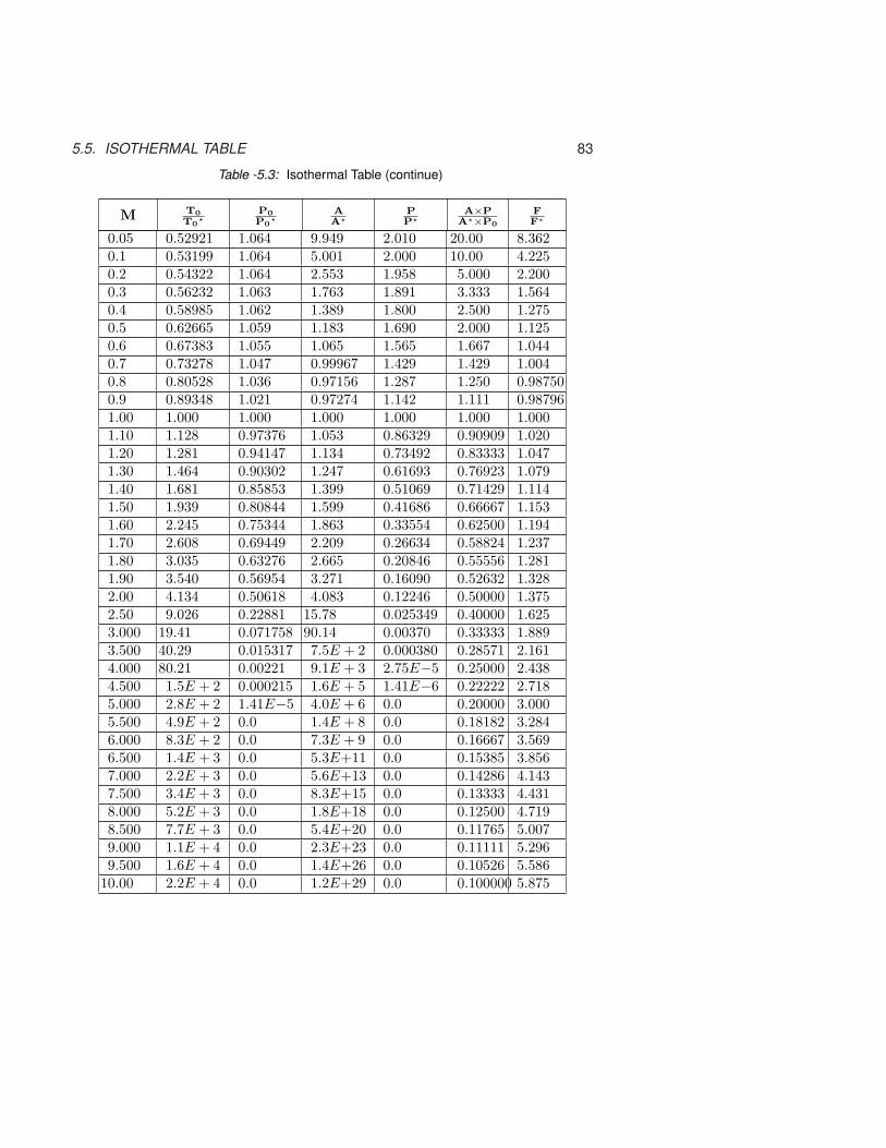
5.5. ISOTHERMAL TABLE 83
Table -5.3: Isothermal Table (continue)
M T0
T0?
P0
P0?
AA?
PP?
A×PA∗×P0
FF∗
0.05 0.52921 1.064 9.949 2.010 20.00 8.3620.1 0.53199 1.064 5.001 2.000 10.00 4.2250.2 0.54322 1.064 2.553 1.958 5.000 2.2000.3 0.56232 1.063 1.763 1.891 3.333 1.5640.4 0.58985 1.062 1.389 1.800 2.500 1.2750.5 0.62665 1.059 1.183 1.690 2.000 1.1250.6 0.67383 1.055 1.065 1.565 1.667 1.0440.7 0.73278 1.047 0.99967 1.429 1.429 1.0040.8 0.80528 1.036 0.97156 1.287 1.250 0.987500.9 0.89348 1.021 0.97274 1.142 1.111 0.987961.00 1.000 1.000 1.000 1.000 1.000 1.0001.10 1.128 0.97376 1.053 0.86329 0.90909 1.0201.20 1.281 0.94147 1.134 0.73492 0.83333 1.0471.30 1.464 0.90302 1.247 0.61693 0.76923 1.0791.40 1.681 0.85853 1.399 0.51069 0.71429 1.1141.50 1.939 0.80844 1.599 0.41686 0.66667 1.1531.60 2.245 0.75344 1.863 0.33554 0.62500 1.1941.70 2.608 0.69449 2.209 0.26634 0.58824 1.2371.80 3.035 0.63276 2.665 0.20846 0.55556 1.2811.90 3.540 0.56954 3.271 0.16090 0.52632 1.3282.00 4.134 0.50618 4.083 0.12246 0.50000 1.3752.50 9.026 0.22881 15.78 0.025349 0.40000 1.6253.000 19.41 0.071758 90.14 0.00370 0.33333 1.8893.500 40.29 0.015317 7.5E + 2 0.000380 0.28571 2.1614.000 80.21 0.00221 9.1E + 3 2.75E−5 0.25000 2.4384.500 1.5E + 2 0.000215 1.6E + 5 1.41E−6 0.22222 2.7185.000 2.8E + 2 1.41E−5 4.0E + 6 0.0 0.20000 3.0005.500 4.9E + 2 0.0 1.4E + 8 0.0 0.18182 3.2846.000 8.3E + 2 0.0 7.3E + 9 0.0 0.16667 3.5696.500 1.4E + 3 0.0 5.3E+11 0.0 0.15385 3.8567.000 2.2E + 3 0.0 5.6E+13 0.0 0.14286 4.1437.500 3.4E + 3 0.0 8.3E+15 0.0 0.13333 4.4318.000 5.2E + 3 0.0 1.8E+18 0.0 0.12500 4.7198.500 7.7E + 3 0.0 5.4E+20 0.0 0.11765 5.0079.000 1.1E + 4 0.0 2.3E+23 0.0 0.11111 5.2969.500 1.6E + 4 0.0 1.4E+26 0.0 0.10526 5.586
10.00 2.2E + 4 0.0 1.2E+29 0.0 0.100000 5.875

84 CHAPTER 5. ISENTROPIC FLOW
5.6 The effects of Real GasesTo obtained expressions for non–ideal gas it is commonly done by reusing the idealgas model and introducing a new variable which is a function of the gas propertieslike the critical pressure and critical temperature. Thus, a real gas equation canbe expressed in equation (4.19). Differentiating equation (4.19) and dividing byequation (4.19) yields
dP
P=
dz
z+
dρ
ρ+
dT
T(5.116)
Again, Gibb’s equation (5.27) is reused to related the entropy change to thechange in thermodynamics properties and applied on non-ideal gas. Since ds = 0and utilizing the equation of the state dh = dP/ρ. The enthalpy is a function of thetemperature and pressure thus, h = h(T, P ) and full differential is
dh =(
∂h
∂T
)
P
dT +(
∂h
∂P
)
T
dP (5.117)
The definition of pressure specific heat is Cp ≡ ∂h∂T and second derivative is
Maxwell relation hence,(
∂h
∂P
)
T
= v − T
(∂s
∂T
)
P
(5.118)
First, the differential of enthalpy is calculated for real gas equation of state as
dh = CpdT −(
T
Z
)(∂z
∂T
)
P
dP
ρ(5.119)
Equations (5.27) and (4.19) are combined to form
ds
R=
Cp
R
dT
T− z
[1 +
(T
Z
)(∂z
∂T
)
P
]dP
P(5.120)
The mechanical energy equation can be expressed as∫
d
(U2
2
)= −
∫dP
ρ(5.121)
At the stagnation the definition requires that the velocity is zero. To carry theintegration of the right hand side the relationship between the pressure and thedensity has to be defined. The following power relationship is assumed
ρ
ρ0=
(P
P0
) 1n
(5.122)

5.6. THE EFFECTS OF REAL GASES 85
Notice, that for perfect gas the n is substituted by k. With integration of equation(5.121) when using relationship which is defined in equation (5.122) results
U2
2=
∫ P1
P0
dP
ρ=
∫ P
P0
1ρ0
(P0
P
) 1n
dP (5.123)
Substituting relation for stagnation density (4.19) results
U2
2=
∫ P
P0
z0RT0
P0
(P0
P
) 1n
dP (5.124)
For n > 1 the integration results in
U =
√√√√z0RT02n
n− 1
[1−
(P
P0
)(n−1n )]
(5.125)
For n = 1 the integration becomes
U =
√2z0RT0 ln
(P0
P
)(5.126)
It must be noted that n is a function of the critical temperature and critical pressure.The mass flow rate is regardless to equation of state as following
m = ρ∗A∗U∗ (5.127)
Where ρ∗ is the density at the throat (assuming the chocking condition) and A∗ isthe cross area of the throat. Thus, the mass flow rate in our properties
m = A∗
ρ∗︷ ︸︸ ︷P0
z0RT0
(P
P0
) 1n
U∗︷ ︸︸ ︷√√√√z0RT02n
n− 1
[1−
(P
P0
)(n−1n )]
(5.128)
For the case of n = 1
m = A∗
ρ∗︷ ︸︸ ︷P0
z0RT0
(P
P0
) 1n
U∗∗︷ ︸︸ ︷√2z0RT0 ln
(P0
P
)(5.129)
The Mach number can be obtained by utilizing equation (4.34) to defined the Machnumber as
M =U√
znRT(5.130)

86 CHAPTER 5. ISENTROPIC FLOW
Integrating equation (5.120) when ds = 0 results
∫ T2
T1
Cp
R
dT
T=
∫ P2
P1
z
(1 +
(T
Z
)(∂z
∂T
)
P
dP
P
)(5.131)
To carryout the integration of equation (5.131) looks at Bernnolli’s equation whichis
∫dU2
2= −
∫dP
ρ(5.132)
After integration of the velocity
dU2
2= −
∫ P/P0
1
ρ0
ρd
(P
P0
)(5.133)
It was shown in Chapter (4) that (4.33) is applicable for some ranges of relativetemperature and pressure (relative to critical temperature and pressure and not thestagnation conditions).
U =
√√√√z0RT0
(2n
n− 1
) [1−
(P
P0
)n−1n
](5.134)
When n = 1 or when n → 1
U =
√2z0RT0 ln
(P0
P
)(5.135)
The mass flow rate for the real gas m = ρ∗U∗A∗
m =A∗P0√z0RT0
√2n
n− 1
(P ∗
P0
) 1n
[1− P ∗
P0
](5.136)
And for n = 1
m =A∗P0√z0RT0
√2n
n− 1
√2z0RT0 ln
(P0
P
)(5.137)
Fliegner’s number in this case is
Fn =mc0
A∗P0
√2n
n− 1
(P ∗
P0
) 1n
[1− P ∗
P0
](5.138)

5.6. THE EFFECTS OF REAL GASES 87
Fliegner’s number for n = 1 is
Fn =mc0
A∗P0= 2
(P ∗
P0
)2
− ln(
P ∗
P0
)(5.139)
The critical ratio of the pressure is
P ∗
P0=
(2
n + 1
) nn−1
(5.140)
When n = 1 or more generally when n → 1 this is a ratio approach
P ∗
P0=√
e (5.141)
To obtain the relationship between the temperature and pressure, equation (5.131)can be integrated
T0
T=
(P0
P
) RCp
[z+T( ∂z∂T )
P]
(5.142)
The power of the pressure ratio is approaching k−1k when z approaches 1. Note
that
T0
T=
(z0
z
)(P0
P
) 1−nn
(5.143)
The Mach number at every point at the nozzle can be expressed as
M =
√√√√(
2n− 1
)z0
z
T0
T
[1−
(P − 0
P
) 1−nn
](5.144)
For n = 1 the Mach number is
M =
√2z0
z
T0
Tln
P0
P(5.145)
The pressure ratio at any point can be expressed as a function of the Mach numberas
T0
T=
[1 +
n− 12
M2
](n−1n )[z+T( ∂z
∂T )P]
(5.146)
for n = 1
T0
T= eM2[z+T( ∂z
∂T )P] (5.147)

88 CHAPTER 5. ISENTROPIC FLOW
The critical temperature is given by
T ∗
T0=
(1 + n
2
)( n1−n )[z+T( ∂z
∂T )P]
(5.148)
and for n = 1
T ∗
T0=
√e−[z+T( ∂z
∂T )P] (5.149)
The mass flow rate as a function of the Mach number is
m =P0n
c0M
√(1 +
n− 12
M2
) n+1n−1
(5.150)
For the case of n = 1 the mass flow rate is
m =P0A
∗nc0
√eM2
√(1 +
n− 12
M2
) n+1n−1
(5.151)
Example 5.9:A design is required that at a specific point the Mach number should be M = 2.61,the pressure 2[Bar], and temperature 300K.
i. Calculate the area ratio between the point and the throat.
ii. Calculate the stagnation pressure and the stagnation temperature.
iii. Are the stagnation pressure and temperature at the entrance different from thepoint? You can assume that k = 1.405.
SOLUTION
1. The solution is simplified by using Potto-GDC for M = 2.61 the results are
M TT0
ρρ0
AA?
PP0
A×PA∗×P0
2.6100 0.42027 0.11761 2.9066 0.04943 0.14366
2. The stagnation pressure is obtained from
P0 =P0
PP =
2.610.04943
∼ 52.802[Bar]
The stagnation temperature is
T0 =T0
TT =
3000.42027
∼ 713.82K
3. Of course, the stagnation pressure is constant for isentropic flow.
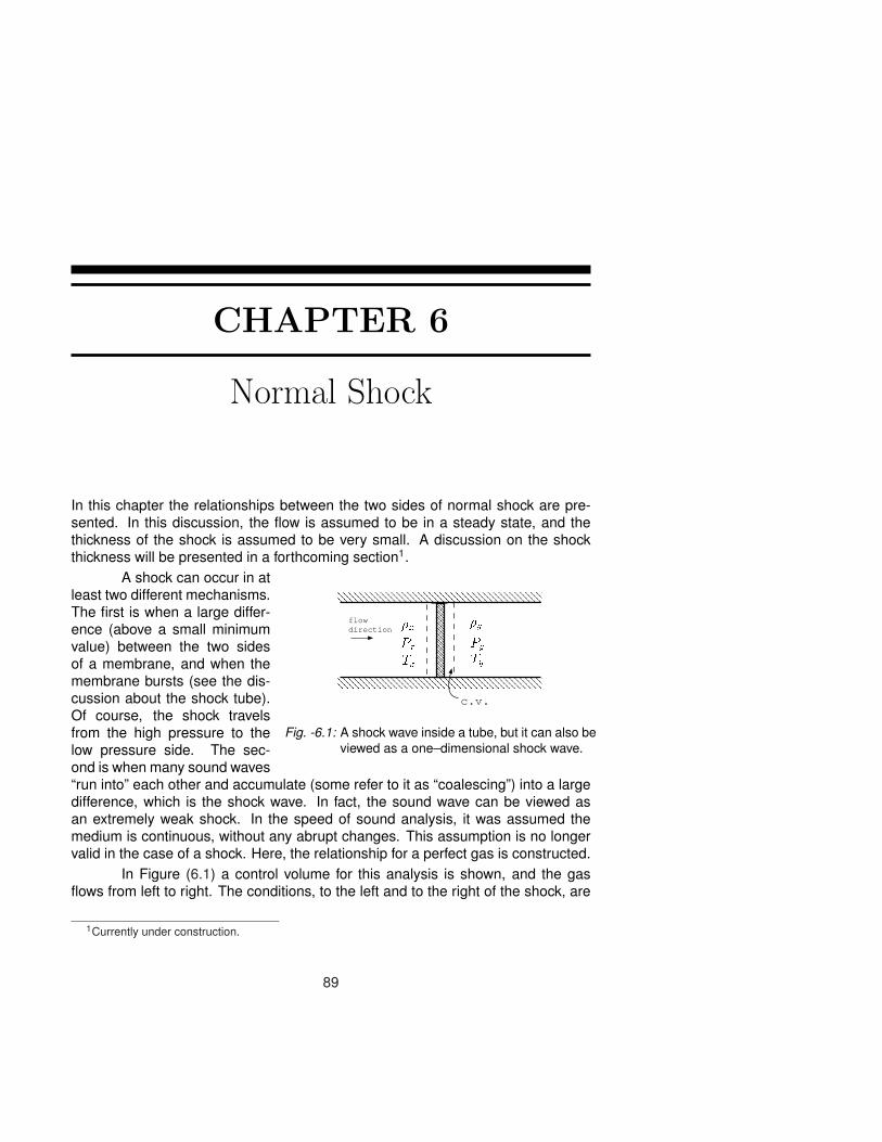
CHAPTER 6
Normal Shock
In this chapter the relationships between the two sides of normal shock are pre-sented. In this discussion, the flow is assumed to be in a steady state, and thethickness of the shock is assumed to be very small. A discussion on the shockthickness will be presented in a forthcoming section1.
�xPx �yPyTx Tyc.v.
flowdirection
Fig. -6.1: A shock wave inside a tube, but it can also beviewed as a one–dimensional shock wave.
A shock can occur in atleast two different mechanisms.The first is when a large differ-ence (above a small minimumvalue) between the two sidesof a membrane, and when themembrane bursts (see the dis-cussion about the shock tube).Of course, the shock travelsfrom the high pressure to thelow pressure side. The sec-ond is when many sound waves“run into” each other and accumulate (some refer to it as “coalescing”) into a largedifference, which is the shock wave. In fact, the sound wave can be viewed asan extremely weak shock. In the speed of sound analysis, it was assumed themedium is continuous, without any abrupt changes. This assumption is no longervalid in the case of a shock. Here, the relationship for a perfect gas is constructed.
In Figure (6.1) a control volume for this analysis is shown, and the gasflows from left to right. The conditions, to the left and to the right of the shock, are
1Currently under construction.
89

90 CHAPTER 6. NORMAL SHOCK
assumed to be uniform2. The conditions to the right of the shock wave are uniform,but different from the left side. The transition in the shock is abrupt and in a verynarrow width.
The chemical reactions (even condensation) are neglected, and the shockoccurs at a very narrow section. Clearly, the isentropic transition assumption is notappropriate in this case because the shock wave is a discontinued area. Therefore,the increase of the entropy is fundamental to the phenomenon and the understand-ing of it.
It is further assumed that there is no friction or heat loss at the shock(because the heat transfer is negligible due to the fact that it occurs on a relativelysmall surface). It is customary in this field to denote x as the upstream conditionand y as the downstream condition.
The mass flow rate is constant from the two sides of the shock and there-fore the mass balance is reduced to
ρxUx = ρyUy (6.1)
In a shock wave, the momentum is the quantity that remains constant be-cause there are no external forces. Thus, it can be written that
Px − Py =(ρxUy
2 − ρyUx2)
(6.2)
The process is adiabatic, or nearly adiabatic, and therefore the energy equationcan be written as
CpTx +Ux
2
2= CpTy +
Uy2
2(6.3)
The equation of state for perfect gas reads
P = ρRT (6.4)
If the conditions upstream are known, then there are four unknown con-ditions downstream. A system of four unknowns and four equations is solvable.Nevertheless, one can note that there are two solutions because of the quadraticof equation (6.3). These two possible solutions refer to the direction of the flow.Physics dictates that there is only one possible solution. One cannot deduce thedirection of the flow from the pressure on both sides of the shock wave. The onlytool that brings us to the direction of the flow is the second law of thermodynamics.This law dictates the direction of the flow, and as it will be shown, the gas flowsfrom a supersonic flow to a subsonic flow. Mathematically, the second law is ex-pressed by the entropy. For the adiabatic process, the entropy must increase. Inmathematical terms, it can be written as follows:
sy − sx > 0 (6.5)2Clearly the change in the shock is so significant compared to the changes in medium before and
after the shock that the changes in the mediums (flow) can be considered uniform.

91
Note that the greater–equal signs were not used. The reason is that the processis irreversible, and therefore no equality can exist. Mathematically, the parametersare P, T, U, and ρ, which are needed to be solved. For ideal gas, equation (6.5) is
lnTy
Tx− (k − 1)
Py
Px> 0 (6.6)
It can also be noticed that entropy, s, can be expressed as a function ofthe other parameters. Now one can view these equations as two different subsetsof equations. The first set is the energy, continuity, and state equations, and thesecond set is the momentum, continuity, and state equations. The solution of ev-ery set of these equations produces one additional degree of freedom, which willproduce a range of possible solutions. Thus, one can have a whole range of solu-tions. In the first case, the energy equation is used, producing various resistanceto the flow. This case is called Fanno flow, and Chapter (10) deals extensively withthis topic. The mathematical explanation is given Chapter (10) in greater detail. In-stead of solving all the equations that were presented, one can solve only four (4)equations (including the second law), which will require additional parameters. Ifthe energy, continuity, and state equations are solved for the arbitrary value of theTy, a parabola in the T − −s diagram will be obtained. On the other hand, whenthe momentum equation is solved instead of the energy equation, the degree offreedom is now energy, i.e., the energy amount “added” to the shock. This situa-tion is similar to a frictionless flow with the addition of heat, and this flow is knownas Rayleigh flow. This flow is dealt with in greater detail in Chapter (11).
s
T
subsonicflow
supersonicflow
RayleighlineFanno
line
shock jump
M < 1
M > 1
Ty; ; Py; sy
Tx; Px; sx
M = 1M = 1
M = 1pk
Fig. -6.2: The intersection of Fanno flow and Rayleigh flowproduces two solutions for the shock wave.
Since the shock hasno heat transfer (a specialcase of Rayleigh flow) andthere isn’t essentially anymomentum transfer (a spe-cial case of Fanno flow),the intersection of thesetwo curves is what reallyhappened in the shock. InFigure (6.2), the intersec-tion is shown and two solu-tions are obtained. Clearly,the increase of the entropydetermines the direction ofthe flow. The entropy in-creases from point x topoint y. It is also worth not-ing that the temperature at M = 1 on Rayleigh flow is larger than that on the Fannoline.

92 CHAPTER 6. NORMAL SHOCK
6.1 Solution of the Governing Equations6.1.1 Informal Model
Accepting the fact that the shock is adiabatic or nearly adiabatic requires that totalenergy is conserved, T0x = T0y. The relationship between the temperature andthe stagnation temperature provides the relationship of the temperature for bothsides of the shock.
Ty
Tx=
Ty
T0y
Tx
T0x
=1 + k−1
2 Mx2
1 + k−12 My
2 (6.7)
All the other relationships are essentially derived from this equation. Theonly issue left to derive is the relationship between Mx and My. Note that the Machnumber is a function of temperature, and thus for known Mx all the other quantitiescan be determined, at least, numerically. The analytical solution is discussed inthe next section.
6.1.2 Formal Model
Equations (6.1), (6.2), and (6.3) can be converted into a dimensionless form. Thereason that dimensionless forms are heavily used in this book is because by doingso it simplifies and clarifies the solution. It can also be noted that in many casesthe dimensionless equations set is more easily solved.
From the continuity equation (6.1) substituting for density, ρ, the equationof state yields
Px
RTxUx =
Py
RTyUy (6.8)
Squaring equation (6.8) results in
Px2
R2Tx2 Ux
2 =Py
2
R2Ty2 Uy
2 (6.9)
Multiplying the two sides by the ratio of the specific heat, k, provides a way toobtain the speed of sound definition/equation for perfect gas, c2 = kRT to be usedfor the Mach number definition, as follows:
Px2
Tx kRTx︸ ︷︷ ︸cx
2
Ux2 =
Py2
Ty kRTy︸ ︷︷ ︸cy
2
Uy2 (6.10)
Note that the speed of sound on the different sides of the shock is different. Utiliz-ing the definition of Mach number results in
Px2
TxMx
2 =Py
2
TyMy
2 (6.11)

6.1. SOLUTION OF THE GOVERNING EQUATIONS 93
Rearranging equation (6.11) results in
Ty
Tx=
(Py
Px
)2 (My
Mx
)2
(6.12)
Energy equation (6.3) can be converted to a dimensionless form which can beexpressed as
Ty
(1 +
k − 12
My2
)= Tx
(1 +
k − 12
Mx2
)(6.13)
It can also be observed that equation (6.13) means that the stagnation temper-ature is the same, T0y = T0x. Under the perfect gas model, ρU2 is identical tokPM2 because
ρU2 =
ρ︷︸︸︷P
RT
M2
︷ ︸︸ ︷
U2
kRT︸︷︷︸c2
kRT = kPM2 (6.14)
Using the identity (6.14) transforms the momentum equation (6.2) into
Px + kPxMx2 = Py + kPyMy
2 (6.15)
Rearranging equation (6.15) yields
Py
Px=
1 + kMx2
1 + kMy2 (6.16)
The pressure ratio in equation (6.16) can be interpreted as the loss of the staticpressure. The loss of the total pressure ratio can be expressed by utilizing therelationship between the pressure and total pressure (see equation (5.11)) as
P0y
P0x
=Py
(1 + k−1
2 My2) k
k−1
Px
(1 + k−1
2 Mx2) k
k−1(6.17)
The relationship between Mx and My is needed to be solved from the above setof equations. This relationship can be obtained from the combination of mass,momentum, and energy equations. From equation (6.13) (energy) and equation(6.12) (mass) the temperature ratio can be eliminated.
(PyMy
PxMx
)2
=1 + k−1
2 Mx2
1 + k−12 My
2 (6.18)

94 CHAPTER 6. NORMAL SHOCK
Combining the results of (6.18) with equation (6.16) results in(
1 + kMx2
1 + kMy2
)2
=(
Mx
My
)2 1 + k−12 Mx
2
1 + k−12 My
2 (6.19)
Equation (6.19) is a symmetrical equation in the sense that if My is substitutedwith Mx and Mx substituted with My the equation remains the same. Thus, onesolution is
My = Mx (6.20)
It can be observed that equation (6.19) is biquadratic. According to the GaussBiquadratic Reciprocity Theorem this kind of equation has a real solution in a cer-tain range3 which will be discussed later. The solution can be obtained by rewritingequation (6.19) as a polynomial (fourth order). It is also possible to cross–multiplyequation (6.19) and divide it by
(Mx
2 −My2)
results in
1 +k − 1
2(My
2 + My2)− kMy
2My2 = 0 (6.21)
Equation (6.21) becomes
My2 =
Mx2 + 2
k−12k
k−1Mx2 − 1
(6.22)
The first solution (6.20) is the trivial solution in which the two sides are identicaland no shock wave occurs. Clearly, in this case, the pressure and the temperaturefrom both sides of the nonexistent shock are the same, i.e. Tx = Ty, Px = Py. Thesecond solution is where the shock wave occurs.
The pressure ratio between the two sides can now be as a function of onlya single Mach number, for example, Mx. Utilizing equation (6.16) and equation(6.22) provides the pressure ratio as only a function of the upstream Mach numberas
Py
Px=
2k
k + 1Mx
2 − k − 1k + 1
or
Py
Px= 1 +
2k
k + 1(Mx
2 − 1)
(6.23)
The density and upstream Mach number relationship can be obtained inthe same fashion to became
ρy
ρx=
Ux
Uy=
(k + 1)Mx2
2 + (k − 1)Mx2 (6.24)
3Ireland, K. and Rosen, M. ”Cubic and Biquadratic Reciprocity.” Ch. 9 in A Classical Introduction toModern Number Theory, 2nd ed. New York: Springer-Verlag, pp. 108-137, 1990.

6.1. SOLUTION OF THE GOVERNING EQUATIONS 95
The fact that the pressure ratio is a function of the upstream Mach number, Mx,provides additional way of obtaining an additional useful relationship. And the tem-perature ratio, as a function of pressure ratio, is transformed into
Ty
Tx=
(Py
Px
) (k+1k−1 + Py
Px
1 + k+1k−1
Py
Px
)(6.25)
In the same way, the relationship between the density ratio and pressure ratio is
ρx
ρy=
1 +(
k+1k−1
)(Py
Px
)(
k+1k−1
)+
(Py
Px
) (6.26)
which is associated with the shock wave.
1 2 3 4 5 6 7 8 9 10M
x
0
0.1
0.2
0.3
0.4
0.5
0.6
0.7
0.8
0.9
1
My
My
P0y
/P0x
Shock Wave relationshipM
y and P
0y/P
0x as a function of M
x
Fri Jun 18 15:47:34 2004
Fig. -6.3: The exit Mach number and the stagnationpressure ratio as a function of upstreamMach number.
The Maximum Conditions
The maximum speed of soundis when the highest tempera-ture is achieved. The maxi-mum temperature that can beachieved is the stagnation tem-perature
Umax =
√2k
k − 1RT0 (6.27)
The stagnation speed of soundis
c0 =√
kRT0 (6.28)
Based on this definition a newMach number can be defined
M0 =U
c0(6.29)
The Star Conditions
The speed of sound at the critical condition can also be a good reference velocity.The speed of sound at that velocity is
c∗ =√
kRT ∗ (6.30)

96 CHAPTER 6. NORMAL SHOCK
In the same manner, an additional Mach number can be defined as
M∗ =U
c∗(6.31)
6.1.3 Prandtl’s Condition
It can be easily observed that the temperature from both sides of the shock waveis discontinuous. Therefore, the speed of sound is different in these adjoiningmediums. It is therefore convenient to define the star Mach number that will beindependent of the specific Mach number (independent of the temperature).
M∗ =U
c∗=
c
c∗U
c=
c
c∗M (6.32)
The jump condition across the shock must satisfy the constant energy.
c2
k − 1+
U2
2=
c∗2
k − 1+
c∗2
2=
k + 12(k − 1)
c∗2 (6.33)
Dividing the mass equation by the momentum equation and combining it with theperfect gas model yields
c12
kU1+ U1 =
c22
kU2+ U2 (6.34)
Combining equation (6.33) and (6.34) results in
1kU1
[k + 1
2c∗2 − k − 1
2U1
]+ U1 =
1kU2
[k + 1
2c∗2 − k − 1
2U2
]+ U2 (6.35)
After rearranging and diving equation (6.35) the following can be obtained:
U1U2 = c∗2 (6.36)
or in a dimensionless form
M∗1M
∗2 = c∗2 (6.37)

6.2. OPERATING EQUATIONS AND ANALYSIS 97
6.2 Operating Equations and AnalysisIn Figure (6.3), the Mach number after the shock, My, and the ratio of the totalpressure, P0y/P0x, are plotted as a function of the entrance Mach number. Theworking equations were presented earlier. Note that the My has a minimum valuewhich depends on the specific heat ratio. It can be noticed that the density ratio(velocity ratio) also has a finite value regardless of the upstream Mach number.The typical situations in which these equations can be used also include the mov-ing shocks. The equations should be used with the Mach number (upstream ordownstream) for a given pressure ratio or density ratio (velocity ratio). This kind ofequations requires examining Table (6.1) for k = 1.4 or utilizing Potto-GDC for forvalue of the specific heat ratio. Finding the Mach number for a pressure ratio of8.30879 and k = 1.32 and is only a few mouse clicks away from the following table.
Mx MyTy
Tx
ρy
ρx
Py
Px
P0y
P0x
2.7245 0.47642 2.1110 3.9360 8.3088 0.38109
1 2 3 4 5 6 7 8 9 10M
x
0.0
10.0
20.0
30.0
40.0
50.0
60.0
70.0
80.0
90.0
100.0
110.0
120.0
Py/P
x
Ty/T
x
ρy/ρ
x
Shock Wave relationshipP
y/P
y, ρ
y/ρ
x and T
y/T
x as a function of M
x
Fri Jun 18 15:48:25 2004
Fig. -6.4: The ratios of the static properties of the two sidesof the shock.
To illustrate the use of theabove equations, an exam-ple is provided.
Example 6.1:Air flows with a Mach num-ber of Mx = 3, at a pres-sure of 0.5 [bar] and atemperature of 0◦C goesthrough a normal shock.Calculate the temperature,pressure, total pressure,and velocity downstream ofthe shock. Assume thatk = 1.4.
SOLUTIONAnalysis:First, the known informa-tion are Mx = 3, Px = 1.5[bar] and Tx = 273K. Using these data, the total pres-sure can be obtained (through an isentropic relationship in Table (5.2), i.e., P0x isknown). Also with the temperature, Tx, the velocity can readily be calculated. Therelationship that was calculated will be utilized to obtain the ratios for the down-stream of the normal shock. Px
P0x= 0.0272237 =⇒ P0x = 1.5/0.0272237 = 55.1[bar]
cx =√
kRTx =√
1.4× 287× 273 = 331.2m/sec
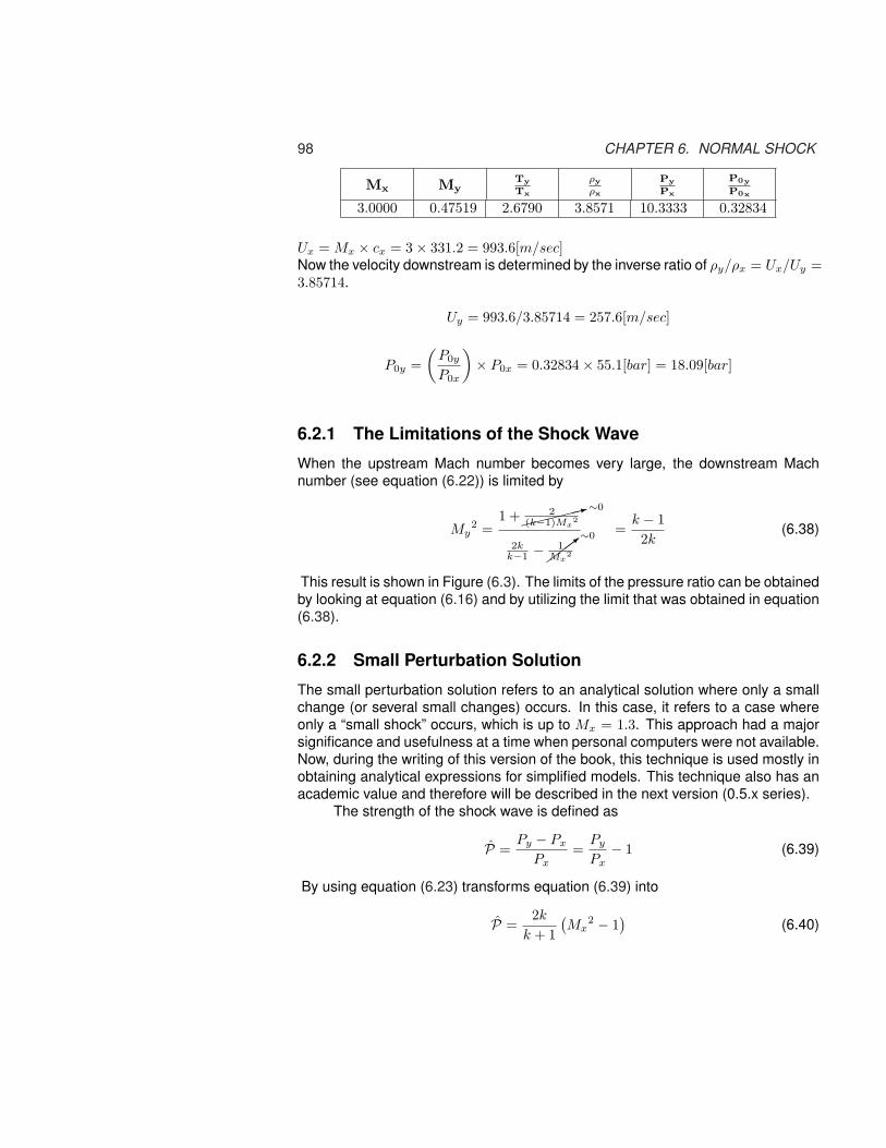
98 CHAPTER 6. NORMAL SHOCK
Mx MyTy
Tx
ρy
ρx
Py
Px
P0y
P0x
3.0000 0.47519 2.6790 3.8571 10.3333 0.32834
Ux = Mx × cx = 3× 331.2 = 993.6[m/sec]Now the velocity downstream is determined by the inverse ratio of ρy/ρx = Ux/Uy =3.85714.
Uy = 993.6/3.85714 = 257.6[m/sec]
P0y =(
P0y
P0x
)× P0x = 0.32834× 55.1[bar] = 18.09[bar]
6.2.1 The Limitations of the Shock Wave
When the upstream Mach number becomes very large, the downstream Machnumber (see equation (6.22)) is limited by
My2 =
1 +»»»»»:∼02(k−1)Mx
2
2kk−1 −½
½½>∼0
1Mx
2
=k − 12k
(6.38)
This result is shown in Figure (6.3). The limits of the pressure ratio can be obtainedby looking at equation (6.16) and by utilizing the limit that was obtained in equation(6.38).
6.2.2 Small Perturbation Solution
The small perturbation solution refers to an analytical solution where only a smallchange (or several small changes) occurs. In this case, it refers to a case whereonly a “small shock” occurs, which is up to Mx = 1.3. This approach had a majorsignificance and usefulness at a time when personal computers were not available.Now, during the writing of this version of the book, this technique is used mostly inobtaining analytical expressions for simplified models. This technique also has anacademic value and therefore will be described in the next version (0.5.x series).
The strength of the shock wave is defined as
P =Py − Px
Px=
Py
Px− 1 (6.39)
By using equation (6.23) transforms equation (6.39) into
P =2k
k + 1(Mx
2 − 1)
(6.40)

6.2. OPERATING EQUATIONS AND ANALYSIS 99
or by utilizing equation (6.24) the following is obtained:
P =2k
k−1
(ρy
ρx − 1)
2k−1 −
(ρy
ρx− 1
) (6.41)
6.2.3 Shock Thickness
The issue of shock thickness (which will be presented in a later version) is pre-sented here for completeness. This issue has a very limited practical applicationfor most students; however, to convince the students that indeed the assumptionof very thin shock is validated by analytical and experimental studies, the issueshould be presented.
The shock thickness can be defined in several ways. The most commondefinition is by passing a tangent to the velocity at the center and finding out wherethe theoretical upstream and downstream conditions are meet.
6.2.4 Shock or Wave Drag
It is communally believed that regardless to the cause of the shock, the shockcreates a drag (due to increase of entropy). In this section, the first touch of thisphenomenon will be presented. The fact that it is assumed that the flow is friction-less does not change whether or not shock drag occur. This explanation is brokeninto two sections: one for stationary shock wave, two for moving shock shock wave.A better explanation should appear in the oblique shock chapter.
Consider a normal shock as shown in figure (6.5). Gas flows in a supersonic
stream lines
ρ2
U2
A2
P2
ρ1
U1
A1
P1
Fig. -6.5: The diagram that reexplains the shock drag effect.
velocity around a two–dimensional body and creates a shock. This shock is anoblique shock, however in this discussion, if the control volume is chosen closeenough to the body is can be considered as almost a normal shock (in the obliqueshock chapter a section on this issue will be presented that explains the fact thatshock is oblique, to be irrelevant).
The control volume that is used here is along two stream lines. The other twoboundaries are arbitrary but close enough to the body. Along the stream lines there

100 CHAPTER 6. NORMAL SHOCK
is no mass exchange and therefore there is no momentum exchange. Moreover,it is assumed that the gas is frictionless, therefore no friction occurs along anystream line. The only change is two arbitrary surfaces since the pressure, velocity,and density are changing. The velocity is reduced Ux > Uy. However, the density isincreasing, and in addition, the pressure is increasing. So what is the momentumnet change in this situation? To answer this question, the momentum equationmust be written and it will be similar to equation (5.104). However, since Fy
F∗ = Fx
F∗there is no net force acting on the body. For example, consider upstream of Mx =3. and for which
Mx MyTy
Tx
ρy
ρx
Py
Px
P0y
P0x
3.0000 0.47519 2.6790 3.8571 10.3333 0.32834
and the corespondent Isentropic information for the Mach numbers is
M TT0
ρρ0
AA?
PP0
A×PA∗×P0
FF∗
3.0000 0.35714 0.07623 4.2346 0.02722 0.11528 0.653260.47519 0.95679 0.89545 1.3904 0.85676 1.1912 0.65326
Now, after it was established, it is not a surprising result. After all, the shockanalysis started with the assumption that no momentum is change. As conclusionthere is no shock drag at stationary shock. This is not true for moving shock as itwill be discussed in section (6.3.1).
6.3 The Moving ShocksIn some situations, the shock wave is not stationary. This kind of situation arises inmany industrial applications. For example, when a valve is suddenly 4 closed anda shock propagates upstream. On the other extreme, when a valve is suddenlyopened or a membrane is ruptured, a shock occurs and propagates downstream(the opposite direction of the previous case). In some industrial applications, aliquid (metal) is pushed in two rapid stages to a cavity through a pipe system. Thisliquid (metal) is pushing gas (mostly) air, which creates two shock stages. As ageneral rule, the shock can move downstream or upstream. The last situation is themost general case, which this section will be dealing with. There are more generacases where the moving shock is created which include a change in the physicalproperties, but this book will not deal with them at this stage. The reluctance to dealwith the most general case is due to fact it is highly specialized and complicatedeven beyond early graduate students level. In these changes (of opening a valveand closing a valve on the other side) create situations in which different shocks aremoving in the tube. The general case is where two shocks collide into one shock
4It will be explained using dimensional analysis what is suddenly open

6.3. THE MOVING SHOCKS 101
and moves upstream or downstream is the general case. A specific example iscommon in die–casting: after the first shock moves a second shock is created inwhich its velocity is dictated by the upstream and downstream velocities.
�xPx�yPy TxTyc.v.
flowdirection
Stationary Coordinates
MxMyUy0 Ux0Us
�x PxPx < Py Us � Ux0!
Txc.v.
Moving Coordinates
Us � Uy0! U = 0Fig. -6.6: Comparison between stationary
shock and moving shock in ducts
In cases where the shock ve-locity can be approximated as a con-stant (in the majority of cases) or asnear constant, the previous analysis,equations, and the tools developed inthis chapter can be employed. Theproblem can be reduced to the pre-viously studied shock, i.e., to the sta-tionary case when the coordinates areattached to the shock front. In such acase, the steady state is obtained inthe moving control value.
For this analysis, the coordi-nates move with the shock. Here, theprime ’ denote the values of the staticcoordinates. Note that this notationis contrary to the conventional nota-tion found in the literature. The rea-son for the deviation is that this choicereduces the programing work (espe-cially for object–oriented programinglike C++). An observer moving withthe shock will notice that the pressurein the shock is
Px
′= Px Py
′= Py (6.42)
The temperature measured by the observer is
Tx
′= Tx Ty
′= Ty (6.43)
Assuming that the shock is moving to the right, (refer to Figure (6.6)) the velocitymeasured by the observer is
Ux = Us − Ux
′(6.44)
Where Us is the shock velocity which is moving to the right. The “downstream”velocity is
Uy
′= Us − Uy (6.45)
The speed of sound on both sides of the shock depends only on the tempera-ture and it is assumed to be constant. The upstream prime Mach number can be
102 CHAPTER 6. NORMAL SHOCK
defined as
Mx
′=
Us − Ux
cx=
Us
cx−Mx = Msx −Mx (6.46)
It can be noted that the additional definition was introduced for the shock upstreamMach number, Msx = Us
cx. The downstream prime Mach number can be expressed
as
My
′=
Us − Uy
cy=
Us
cy−My = Msy −My (6.47)
Similar to the previous case, an additional definition was introduced for the shockdownstream Mach number, Msy. The relationship between the two new shockMach numbers is
Us
cx=
cy
cx
Us
cy
Msx =√
Ty
TxMsy (6.48)
The “upstream” stagnation temperature of the fluid is
T0x = Tx
(1 +
k − 12
Mx2
)
(6.49)
and the “upstream” prime stagnation pressure is
P0x = Px
(1 +
k − 12
Mx2
) kk−1
(6.50)
The same can be said for the “downstream” side of the shock. The differencebetween the stagnation temperature is in the moving coordinates
T0y − T0x = 0 (6.51)
It should be noted that the stagnation temperature (in the stationary coordinates)rises as opposed to the stationary normal shock. The rise in the total temperatureis due to the fact that a new material has entered the c.v. at a very high velocity,and is “converted” or added into the total temperature,
T0y − T0x =Ty
(1 +
k − 12
(Msy −My
′)2)− Tx
(1 +
k − 12
(Msx −Mx
′)2)
0 =
T0y′
︷ ︸︸ ︷Ty
(1 +
k − 12
My
′2)
+TyMsyk − 1
2(Msy − 2My)
−
T0x′
︷ ︸︸ ︷Tx
(1 +
k − 12
Mx
′2)−TxMsx
k − 12
(Msx − 2Mx) (6.52)

6.3. THE MOVING SHOCKS 103
and according to equation (6.51) leads to
T0y
′ − T0x
′= Us
(Tx
cx
k − 12
(Msx − 2Mx)− Ty
cy
k − 12
(Msy − 2My))
(6.53)
Again, this difference in the moving shock is expected because moving materialvelocity (kinetic energy) is converted into internal energy. This difference can alsobe viewed as a result of the unsteady state of the shock.
6.3.1 Shock or Wave Drag Result from a Moving Shock
stream lines
ρ2
U2 6= 0
A2
P2
ρ1
U1 = 0
A1
P1
moving object
stationary lines at thespeed of the object
Fig. -6.7: The diagram that reexplains the shock drag effect of a moving shock.
In section (6.2.4) it was shown that there is no shock drag in stationary shock.However, the shock or wave drag is very significant so much so that at one pointit was considered the sound barrier . Consider the figure (6.7) where the streamlines are moving with the object speed. The other boundaries are stationary but thevelocity at right boundary is not zero. The same arguments, as discussed before inthe stationary case, are applied. What is different in the present case (as oppose tothe stationary shock), one side has increase the momentum of the control volume.This increase momentum in the control volume causes the shock drag. In way, itcan be view as continuous acceleration of the gas around the body from zero. Notethis drag is only applicable to a moving shock (unsteady shock).
The moving shock is either results from a body that moves in gas or from asudden imposed boundary like close or open valve5 In the first case, the forces/energyflows from body to gas and there for there is a need for large force to acceleratethe gas over extremely short distance (shock thickness). In the second case, thegas contains the energy (as high pressure, for example in the open valve case)and the energy potential is lost in the shock process (like shock drag).
5According to my son, the difference between these two cases is the direction of the information.Both case there essentially bodies, however, in one the information flows from inside the field to theboundary while the other case it is the opposite.

104 CHAPTER 6. NORMAL SHOCK
For some strange reasons, this topic has several misconceptions that evenappear in many popular and good textbooks6. Consider the following exampletaken from such a book.
Fig. -6.8: The diagram for the common explanation for shock or wave drag effect a shock.Please notice the strange notations (e.g. V and not U) and they result from averbatim copy.
Example 6.2:A book explains the shock drag is based on the following rational: The body ismoving in a stationary frictionless fluid under one–dimensional flow. The left planeis moving with body at the same speed. The second plane is located “downstreamfrom the body where the gas has expanded isotropically (after the shock wave) tothe upstream static pressure”. the bottom and upper stream line close the controlvolume. Since the pressure is the same on the both planes there is no unbalancedpressure forces. However, there is a change in the momentum in the flow directionbecause U1 > U2. The force is acting on the body. There several mistakes in thisexplanation including the drawing. Explain what is wrong in this description (do notdescribe the error results from oblique shock).
SOLUTIONNeglecting the mistake around the contact of the stream lines with the obliqueshock(see for retouch in the oblique chapter), the control volume suggested isstretched with time. However, the common explanation fall to notice that whenthe isentropic explanation occurs the width of the area change. Thus, the simpleexplanation in a change only in momentum (velocity) is not appropriate. Moreover,in an expanding control volume this simple explanation is not appropriate. Noticethat the relative velocity at the front of the control volume U1 is actually zero. Hence,the claim of U1 > U2 is actually the opposite, U1 < U2.
6Similar situation exist in the surface tension area.

6.3. THE MOVING SHOCKS 105
6.3.2 Shock Result from a Sudden and Complete Stop
The general discussion can be simplified in the extreme case when the shock ismoving from a still medium. This situation arises in many cases in the industry, forexample, in a sudden and complete closing of a valve. The sudden closing of thevalve must result in a zero velocity of the gas. This shock is viewed by some asa reflective shock. The information propagates upstream in which the gas velocityis converted into temperature. In many such cases the steady state is establishedquite rapidly. In such a case, the shock velocity “downstream” is Us. Equations(6.42) to (6.53) can be transformed into simpler equations when Mx is zero and Us
is a positive value.
�xPx �yPyTx Tyc.v.
Stationary Coordinates
Mx My < MxUy0 = 0Ux0 Us �x Px Px < PyUsTx
c.v.Moving Coordinates
Us + Ux0!
Fig. -6.9: Comparison between a stationary shock and a moving shock in a stationarymedium in ducts.
The “upstream” Mach number reads
Mx =Us + Ux
cx= Msx + Mx (6.54)
The “downstream” Mach number reads
My =|Us|cy
= Msy (6.55)
Again, the shock is moving to the left. In the moving coordinates, the observer(with the shock) sees the flow moving from the left to the right. The flow is movingto the right. The upstream is on the left of the shock. The stagnation temperatureincreases by
T0y − T0x = Us
(Tx
cx
k − 12
(Msx + 2Mx) − Ty
cy
k − 12
(Msy))
(6.56)
The prominent question in this situation is what will be the shock wave velocity fora given fluid velocity, Ux
′, and for a given specific heat ratio. The “upstream” or
the “downstream” Mach number is not known even if the pressure and the tem-perature downstream are given. The difficulty lies in the jump from the stationary

106 CHAPTER 6. NORMAL SHOCK
�xPx �yPyTx Tyc.v.
Stationary Coordinates
Mx My < MxUy0 = 0Ux0 Us �x Px Px < PyUsTx
c.v.Moving Coordinates
Us + Ux0!
Fig. -6.10: Comparison between a stationary shock and a moving shock in a stationarymedium in ducts.
coordinates to the moving coordinates. It turns out that it is very useful to use thedimensionless parameter Msx, or Msy instead of the velocity because it combinesthe temperature and the velocity into one parameter.
The relationship between the Mach number on the two sides of the shock are tiedthrough equations (6.54) and (6.55) by
(My)2 =
(Mx
′+ Msx
)2
+ 2k−1
2kk−1
(Mx
′+ Msx
)2 − 1(6.57)
And substituting equation (6.57) into (6.48) results in
Mx =
f(Msx)︷ ︸︸ ︷√Tx
Ty
√√√√(Mx
′+ Msx
)2+ 2
k−1
2kk−1
(Mx
′+ Msx
)2 − 1(6.58)

6.3. THE MOVING SHOCKS 107
0.1 1M
x
0
1
2
3
Msx
Msy
Shock in A Suddenly Close Valvek = 1 4
Thu Aug 3 18:54:21 2006
Fig. -6.11: The moving shock Mach numbers asa result of a sudden and completestop.
The temperature ratio in equation(6.58) and the rest of the right–handside show clearly that Msx has fourpossible solutions (fourth–order poly-nomial Msx has four solutions). Onlyone real solution is possible. The so-lution to equation (6.58) can be ob-tained by several numerical methods.Note, an analytical solution can be ob-tained for equation (6.58) but it seemsutilizing numerical methods is muchmore simple. The typical method isthe “smart” guessing of Msx. For verysmall values of the upstream Machnumber, Mx
′ ∼ ε equation (6.58) pro-vides that Msx ∼ 1 + 1
2ε and Msy =1 − 1
2ε (the coefficient is only approx-imated as 0.5) as shown in Figure(6.11). From the same figure it can also be observed that a high velocity can resultin a much larger velocity for the reflective shock. For example, a Mach numberclose to one (1), which can easily be obtained in a Fanno flow, the result is aboutdouble the sonic velocity of the reflective shock. Sometimes this phenomenon canhave a tremendous significance in industrial applications.
Note that to achieve supersonic velocity (in stationary coordinates) a diverging–converging nozzle is required. Here no such device is needed! Luckily and hope-fully, engineers who are dealing with a supersonic flow when installing the nozzleand pipe systems for gaseous mediums understand the importance of the reflec-tive shock wave.Two numerical methods and the algorithm employed to solve this problem for given,Mx
′, is provided herein:
(a) Guess Mx > 1,
(b) Using shock table or use Potto–GDC to calculate temperature ratio and My,
(c) Calculate the Mx = Mx
′ −√
Tx
TyMy
(d) Compare to the calculated Mx
′to the given Mx
′. and adjust the new guess
Mx > 1 accordingly.
¡p¿ The second method is “successive substitutions,” which has better conver-gence to the solution initially in most ranges but less effective for higher accuracies.
(a) Guess Mx = 1 + Mx
′,

108 CHAPTER 6. NORMAL SHOCK
(b) using the shock table or use Potto–GDC to calculate the temperature ratioand My,
(c) calculate the Mx = Mx
′ −√
Tx
TyMy
(d) Compare the new Mx approach the old Mx, if not satisfactory use the newMx
′to calculate Mx = 1 + Mx
′then return to part (b).
6.3.3 Moving Shock into Stationary Medium (Suddenly OpenValve)
General Velocities Issues
When a valve or membrane is suddenly opened, a shock is created and propagatesdownstream. With the exception of close proximity to the valve, the shock movesin a constant velocity (6.12(a)). Using a coordinates system which moves with theshock results in a stationary shock and the flow is moving to the left see Figure(6.12(b)). The “upstream” will be on the right (see Figure (6.12(b))).
�x PxUx0 = 0 Txc.v.
Uy0Us
(a) Stationary coordinates
�x PxUx = UsTx
c.v.
Uy = Us � Uy0Upstream
(b) Moving coordinates
Fig. -6.12: A shock moves into a still medium as a result of a sudden and complete openingof a valve
Similar definitions of the right side and the left side of the shock Mach numberscan be utilized. It has to be noted that the “upstream” and “downstream” are thereverse from the previous case. The “upstream” Mach number is
Mx =Us
cx= Msx (6.59)
The “downstream” Mach number is
My =Us − Uy
′
cy= Msy −My
′(6.60)
Note that in this case the stagnation temperature in stationary coordinates changes(as in the previous case) whereas the thermal energy (due to pressure difference)

6.3. THE MOVING SHOCKS 109
is converted into velocity. The stagnation temperature (of moving coordinates) is
T0y − T0x = Ty
(1 +
k − 12
(Msy −My)2)− Tx
(1 +
k − 12
(Mx)2)
= 0 (6.61)
A similar rearrangement to the previous case results in
T0y
′ − T0x
′= Ty
(1 +
k − 12
(−2MsyMy + My2)2
)(6.62)
0 10Number of Iteration
0.75
1
1.25
1.5
1.75
Mx
My
Ty/T
x
Shock in A Suddenly Open Valvek = 1 4, M
y’ = 0.3
Wed Aug 23 17:20:59 2006
(a) My′= 0.3
0 5 10 15 20Number of Iteration
0.5
1
1.5
2
2.5
3
3.5
4
Mx
My
Ty/T
x
Shock in A Suddenly Open Valvek = 1 4, M
y’ = 1.3
Wed Aug 23 17:46:15 2006
(b) My′= 1.3
Fig. -6.13: The number of iterations to achieve convergence.
The same question that was prominent in the previous case appears now, what willbe the shock velocity for a given upstream Mach number? Again, the relationshipbetween the two sides is
Msy = My
′+
√√√√ (Msx)2 + 2k−1
2kk−1 (Msx)2 − 1
(6.63)
Since Msx can be represented by Msy theoretically equation (6.63) can be solved.It is common practice to solve this equation by numerical methods. One suchmethods is “successive substitutions.” This method is applied by the following al-gorithm:
(a) Assume that Mx = 1.0.
(b) Calculate the Mach number My by utilizing the tables or Potto–GDC.
(c) Utilizing
Mx =√
Ty
Tx
(My + My
′)
calculate the new “improved” Mx.

110 CHAPTER 6. NORMAL SHOCK
(d) Check the new and improved Mx against the old one. If it is satisfactory, stopor return to stage (b).
To illustrate the convergence of the procedure, consider the case of My
′= 0.3 and
My
′= 0.3. The results show that the convergence occurs very rapidly (see Figure
(6.13)). The larger the value of My
′, the larger number of the iterations required to
achieve the same accuracy. Yet, for most practical purposes, sufficient results canbe achieved after 3-4 iterations.
Piston Velocity When a piston is moving, it creates a shock that moves at aspeed greater than that of the piston itself. The unknown data are the piston veloc-ity, the temperature, and, other conditions ahead of the shock. Therefore, no Machnumber is given but pieces of information on both sides of the shock. In this case,the calculations for Us can be obtained from equation (6.24) that relate the shockvelocities and Shock Mach number as
Ux
Uy=
Msx
Msx − Uy′
cx
=(k + 1)Msx
2
2 + (k − 1)Msx2 (6.64)
Equation (6.64) is a quadratic equation for Msx. There are three solutions ofwhich the first one is Msx = 0 and this is immediately disregarded. The other twosolutions are
Msx =(k + 1)Uy
′ ±√[
Uy′(1 + k)
]2+ 16cx
2
4 cx(6.65)
The negative sign provides a negative value which is disregarded, and the onlysolution left is
Msx =(k + 1)Uy
′+
√[Uy
′(1 + k)
]2+ 16cx
2
4 cx(6.66)
or in a dimensionless form
Msx =(k + 1)Myx
′+
√[Myx
′(1 + k)
]2+ 16
4 (6.67)
Where the “strange” Mach number is Msx
′= Uy
′/cx. The limit of the equation
when cx →∞ leads to
Msx =(k + 1)Myx
′
4(6.68)
As one additional “strange” it can be seen that the shock is close to the pistonwhen the gas ahead of the piston is very hot. This phenomenon occurs in many

6.3. THE MOVING SHOCKS 111
industrial applications, such as the internal combustion engines and die casting.Some use equation (6.68) to explain the next Shock-Choke phenomenon.
In one of the best book in fluid mechanics provides a problem that is thesimilar to the piston pushing but with a twist. In this section analysis will carried forthe error in neglecting the moving shock. This problem is discussed here becauseat first glance looks a simple problem, however, the physics of the problem is a bitcomplicated and deserve a discussion7.
Fig. -6.14: Schematic of showing the piston pushing air.
A piston with a known dimensions (shown in Figure 6.3.3 is pushed by aconstant force. The gas (air) with an initial temperature is pushed through a con-verging nozzle (shown in the original schematic). The point where the movingshock reaches to the exit there are two situations:choked and unchoked flow. If theflow is choked, then the Mach number at the exit is one. If the flow is unchoked,then the exit Mach number is unknown but the pressure ratio is know. Assumingthe flow is choked (see later for the calculation) the exit Mach number is 1 andtherefor, Ue =
√kRT =
√1.4× 287× 0.833× 293.15 ∼ 313[m/sec] The velocity at
the cylinder is assumed to be isentropic and hence area ratio is A/A∗ = 1600 thecondition at the cylinder can be obtained from Potto-GDC as
M TT0
ρρ0
AA?
PP0
A×PA∗×P0
FF∗
3.614E−4 1.0 1.0 1.6E+3 1.0 1.6E+3 6.7E+2
The piston velocity is then Upiston = 0.000361425 × √1.4× 287× 297.15 ∼
0.124[m/sec].Before the semi state state is achieved, the piston is accelerated to the con-
stant velocity (or at least most constant velocity). A this stage, a shock wave ismoving away from piston toward the nozzle. If this shock reaches to exit before thesemi state is achieved, the only way to solve this problem is by a numerical method(either characteristic methods or other numerical method) and it is out of the scopeof this chapter. The transition of the moving shock through the converging nozzleis neglected in this discussion. However, if a quasi steady state is obtained, this
7A student from France forward this problem to this author after argument with his instructor. Theinstructor used the book’s manual solution and refused to accept the student improved solution whichhe learned from this book/author. Therefore, this problem will be referred as the French problem.

112 CHAPTER 6. NORMAL SHOCK
discussion deals with that case. Before the shock is reaching to exit no flow occurat the exit (as opposite to the solution which neglects the moving shock).
The first case (choked, which is the more common, for example, syringewhen pushing air has similar situations), is determined from the fact that pressureat the cylinder can be calculated. If the pressure ratio is equal or higher than thecritical ratio then the flow is choked. For the unchoked case, the exit Mach numberis unknown. However, the pressure ratio between the cylinder and the outsideworld is known. The temperature in the cylinder has to be calculated using movingshock relationship.
In the present case, the critical force should be calculated first. The specificheat ratio is k = 1.4 and therefore critical pressure ratio is 0.528282. The criticalforce is
Fcritical = PcriticalApiston = PaPcritical
PaApiston (6.69)
In this case
Fcritical = 101325(1/0.528282− 1)× π × 0.122
4∼ 1022.74[N ]
Since the force is 1100 [N], it is above the critical force the flow is chocked.The pressure ratio between the cylinder and the choking point is the critical pres-sure ratio. It should be noted that further increase of the force will not change thepressure ratio but the pressure at the choking point (see the Figure below).
Pcylinder
Pa=
101325 + 1100π×0.122
4
101325= 1.96
The moving shock conditions are determined from the velocity of the piston.As first approximation the piston Mach number is obtained from the area ratio inisentropic flow (3.614E−4). Using this Mach number is My
′Potto-GDC provides
Mx My Mx
′My
′ Ty
Tx
Py
Px
P0y
P0x
1.0002 0.99978 0.0 0.000361 1.0 1.001 1.0
The improved the piston pressure ratio (“piston” pressure to the nozzle pres-sure) is changed by only 0.1%. Improved accuracy can be obtained in the seconditeration by taking this shock pressure ratio into consideration. However, here, formost engineering propose this improvement is insignificant. This information pro-vides the ability to calculate the moving shock velocity.
Vshock = cMs = cMx = 1.0002√
1.4× 287× 293.15 ∼ 343.3[m/sec]
The time for the moving shock to reach depends on the length of the cylinder as
t =Lcylinder
Vshock(6.70)
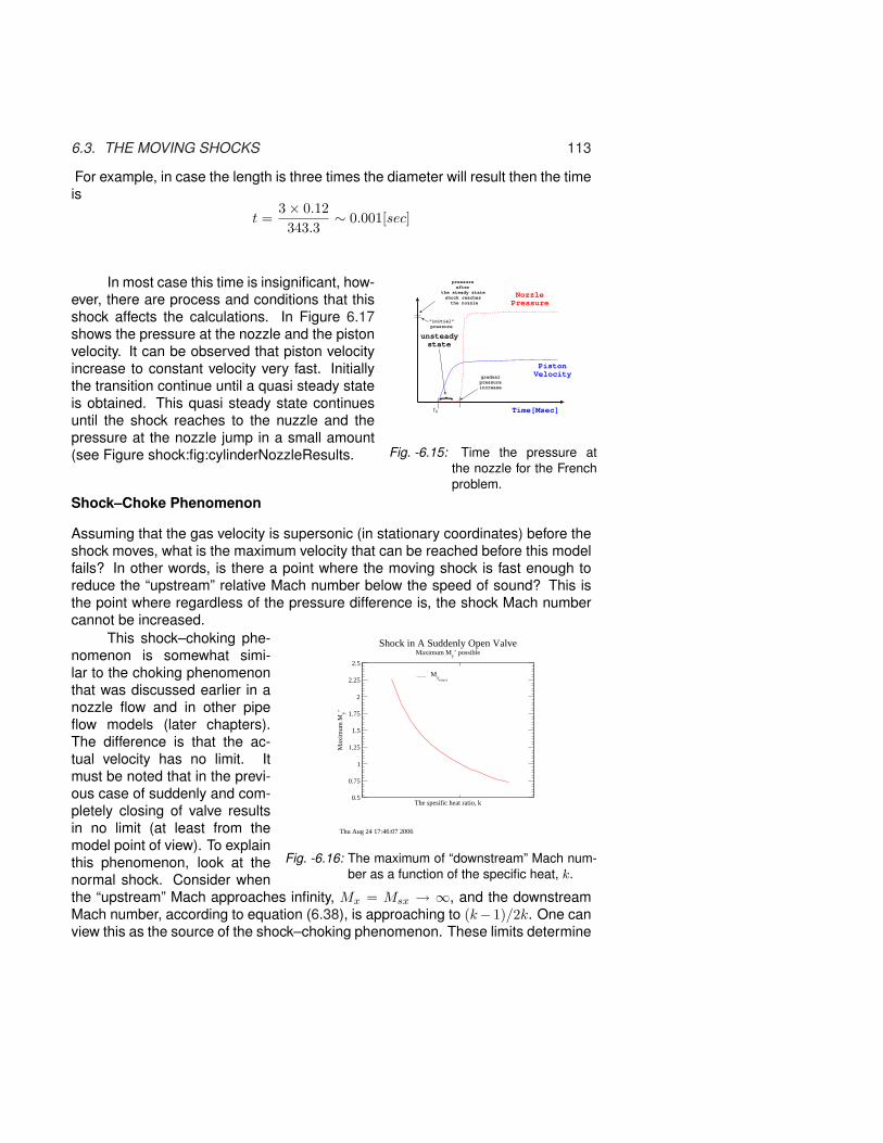
6.3. THE MOVING SHOCKS 113
For example, in case the length is three times the diameter will result then the timeis
t =3× 0.12343.3
∼ 0.001[sec]
NozzlePressure
PistonVelocity
Time[Msec]t0
unsteadystate
{
"initial"pressure
pressureafter
the steady stateshock reaches the nozzle
gradual pressure increase
Fig. -6.15: Time the pressure atthe nozzle for the Frenchproblem.
In most case this time is insignificant, how-ever, there are process and conditions that thisshock affects the calculations. In Figure 6.17shows the pressure at the nozzle and the pistonvelocity. It can be observed that piston velocityincrease to constant velocity very fast. Initiallythe transition continue until a quasi steady stateis obtained. This quasi steady state continuesuntil the shock reaches to the nuzzle and thepressure at the nozzle jump in a small amount(see Figure shock:fig:cylinderNozzleResults.
Shock–Choke Phenomenon
Assuming that the gas velocity is supersonic (in stationary coordinates) before theshock moves, what is the maximum velocity that can be reached before this modelfails? In other words, is there a point where the moving shock is fast enough toreduce the “upstream” relative Mach number below the speed of sound? This isthe point where regardless of the pressure difference is, the shock Mach numbercannot be increased.
The spesific heat ratio, k0.5
0.75
1
1.25
1.5
1.75
2
2.25
2.5
Max
imum
My’
My
(max)
Shock in A Suddenly Open ValveMaximum M
y’ possible
Thu Aug 24 17:46:07 2006
Fig. -6.16: The maximum of “downstream” Mach num-ber as a function of the specific heat, k.
This shock–choking phe-nomenon is somewhat simi-lar to the choking phenomenonthat was discussed earlier in anozzle flow and in other pipeflow models (later chapters).The difference is that the ac-tual velocity has no limit. Itmust be noted that in the previ-ous case of suddenly and com-pletely closing of valve resultsin no limit (at least from themodel point of view). To explainthis phenomenon, look at thenormal shock. Consider whenthe “upstream” Mach approaches infinity, Mx = Msx → ∞, and the downstreamMach number, according to equation (6.38), is approaching to (k−1)/2k. One canview this as the source of the shock–choking phenomenon. These limits determine

114 CHAPTER 6. NORMAL SHOCK
the maximum velocity after the shock since Umax = cyMy. From the upstream side,the Mach number is
Mx = Msx =¡
¡¡¡µ∞√
Ty
Tx
(k − 12k
)(6.71)
Thus, the Mach number is approaching infinity because of the temperature ratiobut the velocity is finite.
To understand this limit, consider that the maximum Mach number is obtainedwhen the pressure ratio is approaching infinity Py
Px→ ∞. By applying equation
(6.23) to this situation the following is obtained:
Msx =
√k + 12k
(Px
Py− 1
)+ 1 (6.72)
and the mass conservation leads to
Uyρy = Usρx(Us − Uy
′)ρy = Usρx
My
′=
√Ty
Tx
(1− ρx
ρy
)Msx (6.73)
Substituting equations (6.26) and (6.25) into equation (6.73) results in
My
′=
1k
(1− Py
Px
) √√√√2k
k+1Py
Px+ k−1
k+1
×
√√√√√1 +
(k+1k−1
)(Py
Px
)(
k+1k−1
)+
(Py
Px
) (6.74)
When the pressure ratio is approaching infinity (extremely strong pressure ratio),the results is
My
′=
√2
k(k − 1)(6.75)
What happens when a gas with a Mach number larger than the maximumMach number possible is flowing in the tube? Obviously, the semi steady statedescribed by the moving shock cannot be sustained. A similar phenomenon tothe choking in the nozzle and later in an internal pipe flow is obtained. The Machnumber is reduced to the maximum value very rapidly. The reduction occurs by anincrease of temperature after the shock or a stationary shock occurs as it will beshown in chapters on internal flow.
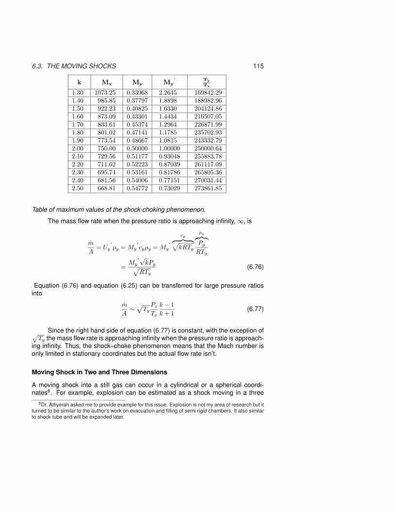
6.3. THE MOVING SHOCKS 115
k Mx My My
′ Ty
Tx
1.30 1073.25 0.33968 2.2645 169842.291.40 985.85 0.37797 1.8898 188982.961.50 922.23 0.40825 1.6330 204124.861.60 873.09 0.43301 1.4434 216507.051.70 833.61 0.45374 1.2964 226871.991.80 801.02 0.47141 1.1785 235702.931.90 773.54 0.48667 1.0815 243332.792.00 750.00 0.50000 1.00000 250000.642.10 729.56 0.51177 0.93048 255883.782.20 711.62 0.52223 0.87039 261117.092.30 695.74 0.53161 0.81786 265805.362.40 681.56 0.54006 0.77151 270031.442.50 668.81 0.54772 0.73029 273861.85
Table of maximum values of the shock-choking phenomenon.
The mass flow rate when the pressure ratio is approaching infinity, ∞, is
m
A= Uy
′ρy = My
′cyρy = My
′
cy︷ ︸︸ ︷√kRTy
ρy︷ ︸︸ ︷Py
RTy
=My
′√kPy√
RTy
(6.76)
Equation (6.76) and equation (6.25) can be transferred for large pressure ratiosinto
m
A∼
√Ty
Px
Tx
k − 1k + 1
(6.77)
Since the right hand side of equation (6.77) is constant, with the exception of√Ty the mass flow rate is approaching infinity when the pressure ratio is approach-
ing infinity. Thus, the shock–choke phenomenon means that the Mach number isonly limited in stationary coordinates but the actual flow rate isn’t.
Moving Shock in Two and Three Dimensions
A moving shock into a still gas can occur in a cylindrical or a spherical coordi-nates8. For example, explosion can be estimated as a shock moving in a three
8Dr. Attiyerah asked me to provide example for this issue. Explosion is not my area of research but itturned to be similar to the author’s work on evacuation and filling of semi rigid chambers. It also similarto shock tube and will be expanded later.

116 CHAPTER 6. NORMAL SHOCK
dimensional direction in uniform way. A long line of explosive can create a cylin-drical moving shock. These shocks are similar to one dimensional shock in whicha moving gas is entering a still gas. In one dimensional shock the velocity of theshock is constant. In two and three dimensions the pressure and shock velocityand velocity behind the shock are function of time. These difference decrease theaccuracy of the calculation because the unsteady part is not accounted for. How-ever, the gain is the simplicity of the calculations. The relationships that have beendeveloped so far for the normal shock are can be used for this case because theshock is perpendicular to the flow. However, it has to be remembered that for verylarge pressure difference the unsteadiness has to be accounted. The deviationincreases as the pressure difference decrease and the geometry became larger.Thus, these result provides the limit for the unsteady state. This principle can bedemonstrated by looking in the following simple example.
Example 6.3:After sometime after an explosion a spherical “bubble” is created with pressureof 20[Bar]. Assume that the atmospheric pressure is 1[Bar] and temperature of27◦C Estimate the higher limit of the velocity of the shock, the velocity of the gasinside the “bubble” and the temperature inside the bubble. Assume that k = 1.4and R = 287[j/kg/K and no chemical reactions occur.
SOLUTIONThe Mach number can be estimated from the pressure ratio
Pinside
Poutside= 20
. One can obtain using Potto–gdc the following
Mx MyTy
Tx
ρy
ρx
Py
Px
P0y
P0x
4.1576 0.43095 4.2975 4.6538 20.0000 0.12155
or by using the shock dynamics section the following
Mx My Mx
′My
′ Ty
Tx
Py
Px
P0y
P0x
4.1576 0.43095 0 1.575 4.298 20 0.12155
The shock velocity estimate is then
Us =
Mx︷︸︸︷Ms cy = 4.1576×√1.4× 287× 300 ∼ 1443.47[m/sec]
The temperature inside the “bubble” is then
Ty =Ty
TxTx = 4.298× 300 ∼ 1289.4K

6.3. THE MOVING SHOCKS 117
The velocity of the gas inside the “bubble” is then
Uy
′= My
′cy = 1.575×√1.4× 287× 1289.4 ∼ 1133.65[m/sec]
These velocities estimates are only the upper limits. The actual velocity will belower due to the unsteadiness of the situation.
End Solution
Uy = Ux
P(t)T(t)
r(t)
Toutside
Poutside
Fig. -6.17: Time the pressure atthe nozzle for the Frenchproblem.
This problem is unsteady state but can be con-sidered as a semi steady state. This kind ofanalysis creates a larger error but gives thetrends and limits. The common problem is thatfor a given pressure ratio and initial radius (vol-ume) the shock velocity and inside gas velocityinside are needed. As first approximation it canbe assumed material inside the “bubble’ is uni-form and undergoes isentropic process. This issimilar to shock tube.
6.3.4 Partially Open Valve
The previous case is a special case of the mov-ing shock. The general case is when one gasflows into another gas with a given velocity. Theonly limitation is that the “downstream’ gas velocity is higher than the “upstream”gas velocity as shown in Figure (6.20).
�x PxUx
′
Txc.v.
Uy0Us
(a) Stationary coordinates
�x PxUx = Us − Ux
′
Txc.v.
Uy = Us � Uy0Upstream
Uy
′
> Ux
′
(b) Moving coordinates
Fig. -6.18: A shock moves into a moving medium as a result of a sudden and complete openvalve.
The relationship between the different Mach numbers on the “upstream” side is
Mx = Msx −Mx
′(6.78)
The relationship between the different Mach on the “downstream” side is
My = Msy −My
′(6.79)

118 CHAPTER 6. NORMAL SHOCK
An additional parameter has be supplied to solve the problem. A common problemis to find the moving shock velocity when the velocity “downstream” or the pressureis suddenly increased. It has to be mentioned that the temperature “downstream”is unknown (the flow of the gas with the higher velocity). The procedure for thecalculations can be done by the following algorithm:
(a) Assume that Mx = Mx
′+ 1.
(b) Calculate the Mach number My by utilizing the tables or Potto–GDC.
(c) Calculate the “downstream” shock Mach number Msy = My + My
′
(d) Utilizing
Mx =√
Ty
Tx(Msy)−Mx
′
calculate the new “improved” Mx
(e) Check the new and improved Mx against the old one. If it is satisfactory, stopor return to stage (b).
0.4 0.8 1.2 1.6 2 2.4 2.8M
y’
0.3
0.4
0.5
0.6
0.7
0.8
0.9
1
My
Mx’ = 0.9
Mx’ = 0.2
Mx’ = 0.0
Shock in A Suddenly Open Valvek = 1 4
Thu Oct 19 10:34:19 2006
Fig. -6.19: The results of the partial open-ing of the valve.
Earlier, it was shown that the shock chok-ing phenomenon occurs when the flow isrunning into a still medium. This phe-nomenon also occurs in the case wherea faster flow is running into a slower fluid.The mathematics is cumbersome but re-sults show that the shock choking phe-nomenon is still there (the Mach number islimited, not the actual flow). Figure (6.19)exhibits some “downstream” Mach num-bers for various static Mach numbers, My
′,
and for various static “upstream” Machnumbers, Mx
′. The figure demonstrates
that the maximum can also occurs in thevicinity of the previous value (see following question/example).
6.3.5 Partially Closed Valve
The totally closed valve is a special case of a partially closed valve in which thereis a sudden change and the resistance increases in the pipe. The informationpropagates upstream in the same way as before. Similar equations can be written:
Ux = Us + Ux
′(6.80)

6.3. THE MOVING SHOCKS 119
�x Px Uy
′
Txc.v.
Ux
′
Us(a) Stationary coordinates
ρy Py
Uy = Us + Uy
′
Ty
c.v.
Ux = Us + Ux
′
Upstream
(b) Moving coordinates
Fig. -6.20: A shock as a result of a sudden and partially a valve closing or a narrowing thepassage to the flow
Uy = Us + Uy
′(6.81)
Mx = Ms + Mx
′(6.82)
My = Ms + My
′(6.83)
For given static Mach numbers the procedure for the calculation is as follows:
(a) Assume that Mx = Mx
′+ 1.
(b) . Calculate the Mach number My by utilizing the tables or Potto–GDC
(c) Calculate the “downstream” shock Mach number Msy = My −My
′
(d) Utilizing
Mx =√
Ty
Tx(Msy) + Mx
′
calculate the new “improved” Mx
(e) Check the new and improved Mx against the old one. If it is satisfactory, stopor return to stage (b).
6.3.6 Worked–out Examples for Shock Dynamics
Example 6.4:A shock is moving at a speed of 450 [m/sec] in a stagnated gas at pressure of1[Bar] and temperature of 27◦C. Compute the pressure and the temperature be-hind the shock. Assume the specific heat ratio is k=1.3.

120 CHAPTER 6. NORMAL SHOCK
SOLUTIONIt can be observed that the gas behind the shock is moving while the gas ahead ofthe shock is still. Thus, it is the case of a shock moving into still medium (suddenlyopened valve case). First, the Mach velocity ahead of the shock has to calculated.
My
′=
U√kRT
=450√
1.3× 287× 300∼ 1.296
By utilizing Potto–GDC or Table (6.4) one can obtain the following table:
Mx My Mx
′My
′ Ty
Tx
Py
Px
P0y
P0x
2.4179 0.50193 0.0 1.296 1.809 6.479 0.49695
Using the above table, the temperature behind the shock is
Ty = Ty
′=
Ty
TxTx = 1.809× 300 ∼ 542.7K
In same manner, it can be done for the pressure ratio as following
Py = Py
′=
Py
PxPx = 6.479× 1.0 ∼ 6.479[Bar]
The velocity behind the shock wave is obtained (for confirmation)
Uy
′= My
′cy = 1.296×√1.3× 287× 542.7 ∼ 450
[ m
sec
]
Example 6.5:Gas flows in a tube with a velocity of 450[m/sec]. The static pressure at the tubeis 2Bar and the (static) temperature of 300K. The gas is brought into a completestop by a sudden closing a valve. Calculate the velocity and the pressure behindthe reflecting shock. The specific heat ratio can be assumed to be k = 1.4.
SOLUTION
The first thing that needs to be done is to find the prime Mach number Mx
′=
1.2961. Then, the prime properties can be found. At this stage the reflecting shockvelocity is unknown.Simply using the Potto–GDC provides for the temperature and velocity the followingtable:
Mx My Mx
′My
′ Ty
Tx
Py
Px
P0y
P0x
2.0445 0.56995 1.2961 0.0 1.724 4.710 0.70009

6.3. THE MOVING SHOCKS 121
If you insist on doing the steps yourself, find the upstream prime Mach, Mx
′to be
1.2961. Then using Table (6.2) you can find the proper Mx. If this detail is notsufficient then simply utilize the iterations procedure described earlier and obtainthe following:
i Mx MyTy
TxMy
′
0 2.2961 0.53487 1.9432 0.01 2.042 0.57040 1.722 0.02 2.045 0.56994 1.724 0.03 2.044 0.56995 1.724 0.04 2.044 0.56995 1.724 0.0
The table was obtained by utilizing Potto–GDC with the iteration request.
Example 6.6:What should be the prime Mach number (or the combination of the velocity withthe temperature, for those who like an additional step) in order to double the tem-perature when the valve is suddenly and totally closed?
SOLUTIONThe ratio can be obtained from Table (6.3). It can also be obtained from the sta-tionary normal shock wave table. Potto-GDC provides for this temperature ratio thefollowing table:
Mx MyTy
Tx
ρy
ρx
Py
Px
P0y
P0x
2.3574 0.52778 2.0000 3.1583 6.3166 0.55832
using the required Mx = 2.3574 in the moving shock table provides
Mx My Mx
′My
′ Ty
Tx
Py
Px
P0y
P0x
2.3574 0.52778 0.78928 0.0 2.000 6.317 0.55830
Example 6.7:A gas is flowing in a pipe with a Mach number of 0.4. Calculate the speed of theshock when a valve is closed in such a way that the Mach number is reduced byhalf. Hint, this is the case of a partially closed valve case in which the ratio of theprime Mach number is half (the new parameter that is added in the general case).
SOLUTIONRefer to section (6.3.5) for the calculation procedure. Potto-GDC provides thesolution of the above data

122 CHAPTER 6. NORMAL SHOCK
Mx My Mx
′My
′ Ty
Tx
Py
Px
P0y
P0x
1.1220 0.89509 0.40000 0.20000 1.0789 1.3020 0.99813
If the information about the iterations is needed please refer to the following table.
i Mx MyTy
Tx
Py
PxMy
′
0 1.4000 0.73971 1.2547 2.1200 0.200001 1.0045 0.99548 1.0030 1.0106 0.200002 1.1967 0.84424 1.1259 1.5041 0.200003 1.0836 0.92479 1.0545 1.2032 0.200004 1.1443 0.87903 1.0930 1.3609 0.200005 1.1099 0.90416 1.0712 1.2705 0.200006 1.1288 0.89009 1.0832 1.3199 0.200007 1.1182 0.89789 1.0765 1.2922 0.200008 1.1241 0.89354 1.0802 1.3075 0.200009 1.1208 0.89595 1.0782 1.2989 0.20000
10 1.1226 0.89461 1.0793 1.3037 0.2000011 1.1216 0.89536 1.0787 1.3011 0.2000012 1.1222 0.89494 1.0790 1.3025 0.2000013 1.1219 0.89517 1.0788 1.3017 0.2000014 1.1221 0.89504 1.0789 1.3022 0.2000015 1.1220 0.89512 1.0789 1.3019 0.2000016 1.1220 0.89508 1.0789 1.3020 0.2000017 1.1220 0.89510 1.0789 1.3020 0.2000018 1.1220 0.89509 1.0789 1.3020 0.2000019 1.1220 0.89509 1.0789 1.3020 0.2000020 1.1220 0.89509 1.0789 1.3020 0.2000021 1.1220 0.89509 1.0789 1.3020 0.2000022 1.1220 0.89509 1.0789 1.3020 0.20000
Example 6.8:
My
′
= 0.8Mx
′
= 0.4
Fig. -6.21: Schematic of a piston pushing air in atube.
A piston is pushing air that flowsin a tube with a Mach number ofM = 0.4 and 300◦C. The piston isaccelerated very rapidly and the airadjoined the piston obtains Machnumber M = 0.8. Calculate the ve-locity of the shock created by thepiston in the air. Calculate the timeit takes for the shock to reach theend of the tube of 1.0m length. Assume that there is no friction and the Fanno flowmodel is not applicable.

6.3. THE MOVING SHOCKS 123
SOLUTIONUsing the procedure described in this section, the solution is
Mx My Mx
′My
′ Ty
Tx
Py
Px
P0y
P0x
1.2380 0.81942 0.50000 0.80000 1.1519 1.6215 0.98860
The complete iteration is provided below.
i Mx MyTy
Tx
Py
PxMy
′
0 1.5000 0.70109 1.3202 2.4583 0.800001 1.2248 0.82716 1.1435 1.5834 0.800002 1.2400 0.81829 1.1531 1.6273 0.800003 1.2378 0.81958 1.1517 1.6207 0.800004 1.2381 0.81940 1.1519 1.6217 0.800005 1.2380 0.81943 1.1519 1.6215 0.800006 1.2380 0.81942 1.1519 1.6216 0.80000
The time it takes for the shock to reach the end of the cylinder is
t =length
Us︸︷︷︸cx(Mx−Mx
′)
=1√
1.4× 287× 300(1.2380− 0.4)= 0.0034[sec]
Example 6.9:From the previous example (6.13) calculate the velocity difference between initialpiston velocity and final piston velocity.
SOLUTIONThe stationary difference between the two sides of the shock is:
∆U =Uy
′ − Ux
′= cyUy
′ − cxUx
′
=√
1.4× 287× 300
0.8×
qTyTx︷ ︸︸ ︷√
1.1519−0.5
∼ 124.4[m/sec]

124 CHAPTER 6. NORMAL SHOCK
Example 6.10:
40 m/sec 70 m/sec
1 [Bar]300 K
shockwaves
Fig. -6.22: Figure for Example (6.10)
An engine is designed so thattwo pistons are moving towardeach other (see Figure (6.22)).The air between the pistons isat 1[Bar] and 300K. The dis-tance between the two pistonsis 1[m]. Calculate the time it willtake for the two shocks to col-lide.
SOLUTIONThis situation is an open valve case where the prime information is given. Thesolution is given by equation (6.66), and, it is the explicit analytical solution. Forthis case the following table can easily be obtain from Potto–GDC for the left piston
Mx My Mx
′My
′ Ty
Tx
Py
Px
P0y
P0xUy
′cx
1.0715 0.93471 0.0 0.95890 1.047 1.173 0.99959 40.0 347.
while the velocity of the right piston is
Mx My Mx
′My
′ Ty
Tx
Py
Px
P0y
P0xUy
′cx
1.1283 0.89048 0.0 0.93451 1.083 1.318 0.99785 70.0 347.
The time for the shocks to collide is
t =length
Usx1 + Usx2
=1[m]
(1.0715 + 1.1283)347.∼ 0.0013[sec]
6.4 Shock TubeThe shock tube is a study tool with very little practical purposes. It is used in manycases to understand certain phenomena. Other situations can be examined andextended from these phenomena. A cylinder with two chambers connected by adiaphragm. On one side the pressure is high, while the pressure on the other sideis low. When the diaphragm is ruptured the gas from the high pressure sectionflows into the low pressure section. When the pressure is high enough, a shockis created that it travels to the low pressure chamber. This is the same case as inthe suddenly opened valve case described previously. At the back of the shock,expansion waves occur with a reduction of pressure. The temperature is known toreach several thousands degrees in a very brief period of time. The high pressurechamber is referred to in the literature is the driver section and the low section isreferred to as the expansion section.

6.4. SHOCK TUBE 125
Diaphragm
expansionfront
distance
t1
t
reflectiveshockwave
Contact Surface
front
back
some wherereflective wave
shock
wave
12345
Fig. -6.23: The shock tube schematic with a pressure”diagram.”
Initially, the gas from the driversection is coalescing from smallshock waves into a large shockwave. In this analysis, it isassumed that this time is es-sentially zero. Zone 1 is anundisturbed gas and zone 2 isan area where the shock al-ready passed. The assumptionis that the shock is very sharpwith zero width. On the otherside, the expansion waves aremoving into the high pressurechamber i.e. the driver section.The shock is moving at a super-sonic speed (it depends on thedefinition, i.e., what referencetemperature is being used) andthe medium behind the shock is also moving but at a velocity, U2, which can besupersonic or subsonic in stationary coordinates. The velocities in the expansionchamber vary between three zones. In zone 3 is the original material that was inthe high pressure chamber but is now the same pressure as zone 2. Zone 4 iswhere the gradual transition occurs between original high pressure to low pres-sure. The boundaries of zone 4 are defined by initial conditions. The expansionfront is moving at the local speed of sound in the high pressure section. The ex-pansion back front is moving at the local speed of sound velocity but the actual gasis moving in the opposite direction in U2. In fact, material in the expansion chamberand the front are moving to the left while the actual flow of the gas is moving to theright (refer to Figure (6.23)). In zone 5, the velocity is zero and the pressure is inits original value.
The properties in the different zones have different relationships. The relationshipbetween zone 1 and zone 2 is that of a moving shock into still medium (again, thisis a case of sudden opened valve). The material in zone 2 and 3 is moving at thesame velocity (speed) but the temperature and the entropy are different, while thepressure in the two zones are the same. The pressure, the temperature and theirproperties in zone 4 aren’t constant and continuous between the conditions in zone3 to the conditions in zone 5. The expansion front wave velocity is larger than thevelocity at the back front expansion wave velocity. Zone 4 is expanding during theinitial stage (until the expansion reaches the wall).
The shock tube is a relatively small length 1− 2[m] and the typical velocity is in therange of the speed of sound, c ∼ √
340 thus the whole process takes only a fewmilliseconds or less. Thus, these kinds of experiments require fast recording de-vices (a relatively fast camera and fast data acquisition devices.). A typical designproblem of a shock tube is finding the pressure to achieve the desired temperature

126 CHAPTER 6. NORMAL SHOCK
or Mach number. The relationship between the different properties was discussedearlier and because it is a common problem, a review of the material is providedthus far.The following equations were developed earlier and are repeated here for clarifica-tion. The pressure ratio between the two sides of the shock is
P2
P1=
k − 1k + 1
(2k
k − 1Ms1
2 − 1)
(6.84)
Rearranging equation (6.84) becomes
Ms1 =√
k − 12k
+k + 12k
P2
P1(6.85)
Or expressing the velocity as
Us = Ms1c1 = c1
√k − 12k
+k + 12k
P2
P1(6.86)
And the velocity ratio between the two sides of the shock is
U1
U2=
ρ2
ρ2=
1 + k+1k−1
P2P1
k+1k−1
P2P1
(6.87)
The fluid velocity in zone 2 is the same
U2′ = Us − U2 = Us
(1− U2
Us
)(6.88)
From the mass conservation, it follows that
U2
Us=
ρ1
ρ2(6.89)
U2
′= c1
√k − 12k
+k + 12k
P2
P1
√√√√1−k+1k−1 + P2
P1
1 + k+1k−1
P2P1
(6.90)
After rearranging equation (6.90) the result is
U2
′=
c1
k
(P2
P1− 1
) √√√√2k
k+1P2P1
k−11+k
(6.91)

6.4. SHOCK TUBE 127
On the isentropic side, in zone 4, taking the derivative of the continuity equation,d(ρU) = 0, and dividing by the continuity equation the following is obtained:
dρ
ρ= −dU
c(6.92)
Since the process in zone 4 is isentropic, applying the isentropic relationship (T ∝ρk−1) yields
c
c5=
√T
T5=
(ρ
ρ5
) k−12
(6.93)
From equation (6.92) it follows that
dU = −cdρ
ρ= c5
(ρ
ρ5
) k−12
dρ (6.94)
Equation (6.94) can be integrated as follows:
∫ U3
U5=0
dU =∫ ρ3
ρ5
c5
(ρ
ρ5
) k−12
dρ (6.95)
The results of the integration are
U3 =2c5
k − 1
(1−
(ρ3
ρ5
) k−12
)(6.96)
Or in terms of the pressure ratio as
U3 =2c5
k − 1
(1−
(P3
P5
) k−12k
)(6.97)
As it was mentioned earlier the velocity at points 2′
and 3 are identical, henceequation (6.97) and equation (6.91) can be combined to yield
2c5
k − 1
(1−
(P3
P5
) k−12k
)=
c1
k
(P2
P1− 1
) √√√√2k
k+1P2P1
k−11+k
(6.98)
After some rearrangement, equation (6.98) is transformed into
P5
P1=
P2
P1
1−
(k − 1) c1c5
(P5P3− 1
)
√2k
√2k + (k + 1)
(P2P1− 1
)
− 2kk−1
(6.99)

128 CHAPTER 6. NORMAL SHOCK
Or in terms of the Mach number, Ms1
P5
P1=
k1 − 1k + 1 + 1
(2k
k1 − 1Ms1
2 − 1) [
1−k−1k+1
c1c5
(Ms1
2 − 1)
Ms1
]− 2kk−1
(6.100)
Using the Rankine–Hugoniot relationship and the perfect gas model, the followingis obtained:
T2
T1=
1 + k1−1k1+1
P2P1
1 + k1−1k1+1
P1P2
(6.101)
By utilizing the isentropic relationship for zone 3 to 5 results in
T3
T5=
(P3
P5
) k5−1k5
=
(P2P1P5P1
) k5−1k5
(6.102)
Example 6.11:A shock tube with an initial pressure ratio of P5
P1= 20 and an initial temperature of
300K. Find the shock velocity and temperature behind the shock if the pressureratio is P5
P1= 40?
SOLUTION
6.5 Shock with Real Gases
6.6 Shock in Wet Steam
6.7 Normal Shock in Ducts
The flow in ducts is related to boundary layer issues. For a high Reynolds number,the assumption of an uniform flow in the duct is closer to reality. It is normal tohave a large Mach number with a large Re number. In that case, the assumptionsin construction of these models are acceptable and reasonable.
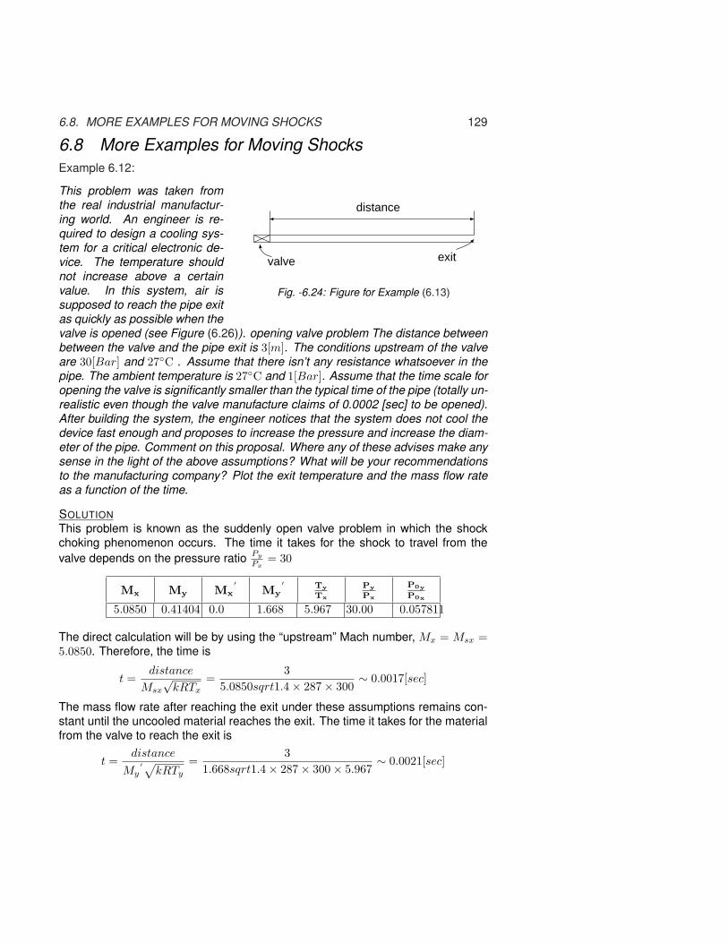
6.8. MORE EXAMPLES FOR MOVING SHOCKS 129
6.8 More Examples for Moving ShocksExample 6.12:
exit
distance
valve
Fig. -6.24: Figure for Example (6.13)
This problem was taken fromthe real industrial manufactur-ing world. An engineer is re-quired to design a cooling sys-tem for a critical electronic de-vice. The temperature shouldnot increase above a certainvalue. In this system, air issupposed to reach the pipe exitas quickly as possible when thevalve is opened (see Figure (6.26)). opening valve problem The distance betweenbetween the valve and the pipe exit is 3[m]. The conditions upstream of the valveare 30[Bar] and 27◦C . Assume that there isn’t any resistance whatsoever in thepipe. The ambient temperature is 27◦C and 1[Bar]. Assume that the time scale foropening the valve is significantly smaller than the typical time of the pipe (totally un-realistic even though the valve manufacture claims of 0.0002 [sec] to be opened).After building the system, the engineer notices that the system does not cool thedevice fast enough and proposes to increase the pressure and increase the diam-eter of the pipe. Comment on this proposal. Where any of these advises make anysense in the light of the above assumptions? What will be your recommendationsto the manufacturing company? Plot the exit temperature and the mass flow rateas a function of the time.
SOLUTIONThis problem is known as the suddenly open valve problem in which the shockchoking phenomenon occurs. The time it takes for the shock to travel from thevalve depends on the pressure ratio Py
Px= 30
Mx My Mx
′My
′ Ty
Tx
Py
Px
P0y
P0x
5.0850 0.41404 0.0 1.668 5.967 30.00 0.057811
The direct calculation will be by using the “upstream” Mach number, Mx = Msx =5.0850. Therefore, the time is
t =distance
Msx
√kRTx
=3
5.0850sqrt1.4× 287× 300∼ 0.0017[sec]
The mass flow rate after reaching the exit under these assumptions remains con-stant until the uncooled material reaches the exit. The time it takes for the materialfrom the valve to reach the exit is
t =distance
My′√
kRTy
=3
1.668sqrt1.4× 287× 300× 5.967∼ 0.0021[sec]

130 CHAPTER 6. NORMAL SHOCK
Velocity
Mass FlowRate
Time[Msec]
Fig. -6.25: The results for Example (6.13)
During that difference of time the ma-terial is get heated instead of coolingdown because of the high temperature.The suggestion of the engineer to in-crease the pressure will decrease thetime but will increase the temperatureat the exit during this critical time pe-riod. Thus, this suggestion contradictsthe purpose of the required manufactur-ing needs.
To increase the pipe diameter will notchange the temperature and thereforewill not change the effects of heating. Itcan only increase the rate after the initial heating spike
A possible solution is to have the valve very close to the pipe exit. Thus, the heatingtime is reduced significantly. There is also the possibility of steps increase in whichevery step heat released will not be enough to over heat the device. The lastpossible requirement a programmable valve and very fast which its valve probablyexceed the moving shock the valve downstream. The plot of the mass flow rateand the velocity are given in Figure (6.27).
Example 6.13:
exit
distance
valve
Fig. -6.26: Figure for example (6.13)
This problem was taken fromthe real industrial manufactur-ing world. Engineer is given todesign a cooling system for crit-ical electronic devise. The tem-perature should not increaseabove certain value. In this sys-tem air is supposed to reach thepipe exit as quickly as possiblewhen the valve is opened (seeFigure (6.26)). The distance between the valve to the exit is 3[m]. The condi-tions upstream the valve are 30[Bar] and 27◦C . Assume that there isn’t resistancewhatsoever in the pipe. The ambient temperature is 27◦C and 1[Bar]. Assume thatthe time scale for opening the valve is significantly smaller than the typical time ofthe pipe (totally unrealistic even though the valve manufacture claims that it takes0.0002 [sec] to open completely the valve). After building the system the engi-neer notices that the system does not cool the device fast enough and proposesto increase the pressure and increase the diameter of the pipe. Comment on thisproposal. Did the suggestions make any sense in the light of the above assump-tions? What will be your recommendations to the manufacturing company? Plotthe exit temperature and mass flow rate as function of the time.

6.8. MORE EXAMPLES FOR MOVING SHOCKS 131
SOLUTIONThis problem is known as the suddenly open valve problem in which the shockchoking phenomenon occurs. The time it takes for the shock to travel from thevalve depends of the pressure ratio Py
Px= 30.
Mx My Mx
′My
′ Ty
Tx
Py
Px
P0y
P0x
5.0850 0.41404 0.0 1.668 5.967 30.00 0.057811
The direct calculation will be by using the “upstream” Mach number, Mx = Msx =5.0850. Therefore, the time is
t =distance
Msx
√kRTx
=3
5.0850sqrt1.4× 287× 300∼ 0.0017[sec]
The mass flow rate after reaching the exit under these assumptions remains con-stant until the uncooled material reaches the exit. The time it takes the materialfrom the valve to reach the exit is
t =distance
My′√
kRTy
=3
1.668sqrt1.4× 287× 300× 5.967∼ 0.0021[sec]
Velocity
Mass FlowRate
Time[Msec]
Fig. -6.27: The results for Example (6.13)
During that difference of time the ma-terial is get heated instead of cold toa high temperature. The suggestion ofthe engineer to increase the pressurewill decrease the time but will increasethe temperature at the exit during thiscritical time period. Thus, this sugges-tion contradicts the purpose of requiredthe manufacturing needs.To increase the pipe diameter will notchange the temperature and thereforewill not change the effects of heating. Itcan only increase the rate after the ini-tial heating spike.A possible solution is to have the valve very close to the pipe exit. Thus, the heatingtime is reduced significantly. There is also the possibility of steps increase in whichevery step heat released will not be enough to over heat the device. The lastpossible requirement programmable value and very fast which its valve probablyexceed the moving shock the valve downstream. The plot of the mass flow rateand the velocity are given in Figure (6.27).
Example 6.14:Example (6.13) deals with a damaging of electronic product by the temperatureincrease. Try to estimate the temperature increase of the product. Plot the pipeexit temperature as a function of the time.

132 CHAPTER 6. NORMAL SHOCK
SOLUTIONTo be developed
6.9 Tables of Normal Shocks, k = 1.4 Ideal Gas
Table -6.1: The shock wave table for k = 1.4
Mx MyTy
Tx
ρy
ρx
Py
Px
P0y
P0x
1.00 1.00000 1.00000 1.00000 1.00000 1.000001.05 0.95313 1.03284 1.08398 1.11958 0.999851.10 0.91177 1.06494 1.16908 1.24500 0.998931.15 0.87502 1.09658 1.25504 1.37625 0.996691.20 0.84217 1.12799 1.34161 1.51333 0.992801.25 0.81264 1.15938 1.42857 1.65625 0.987061.30 0.78596 1.19087 1.51570 1.80500 0.979371.35 0.76175 1.22261 1.60278 1.95958 0.969741.40 0.73971 1.25469 1.68966 2.12000 0.958191.45 0.71956 1.28720 1.77614 2.28625 0.944841.50 0.70109 1.32022 1.86207 2.45833 0.929791.55 0.68410 1.35379 1.94732 2.63625 0.913191.60 0.66844 1.38797 2.03175 2.82000 0.895201.65 0.65396 1.42280 2.11525 3.00958 0.875991.70 0.64054 1.45833 2.19772 3.20500 0.855721.75 0.62809 1.49458 2.27907 3.40625 0.834571.80 0.61650 1.53158 2.35922 3.61333 0.812681.85 0.60570 1.56935 2.43811 3.82625 0.790231.90 0.59562 1.60792 2.51568 4.04500 0.767361.95 0.58618 1.64729 2.59188 4.26958 0.744202.00 0.57735 1.68750 2.66667 4.50000 0.720872.05 0.56906 1.72855 2.74002 4.73625 0.697512.10 0.56128 1.77045 2.81190 4.97833 0.674202.15 0.55395 1.81322 2.88231 5.22625 0.651052.20 0.54706 1.85686 2.95122 5.48000 0.628142.25 0.54055 1.90138 3.01863 5.73958 0.605532.30 0.53441 1.94680 3.08455 6.00500 0.583292.35 0.52861 1.99311 3.14897 6.27625 0.561482.40 0.52312 2.04033 3.21190 6.55333 0.540142.45 0.51792 2.08846 3.27335 6.83625 0.519312.50 0.51299 2.13750 3.33333 7.12500 0.499012.75 0.49181 2.39657 3.61194 8.65625 0.406233.00 0.47519 2.67901 3.85714 10.33333 0.328343.25 0.46192 2.98511 4.07229 12.15625 0.26451

6.9. TABLES OF NORMAL SHOCKS, K = 1.4 IDEAL GAS 133
Table -6.1: The shock wave table for k = 1.4 (continue)
Mx MyTy
Tx
ρy
ρx
Py
Px
P0y
P0x
3.50 0.45115 3.31505 4.26087 14.12500 0.212953.75 0.44231 3.66894 4.42623 16.23958 0.171664.00 0.43496 4.04688 4.57143 18.50000 0.138764.25 0.42878 4.44891 4.69919 20.90625 0.112564.50 0.42355 4.87509 4.81188 23.45833 0.091704.75 0.41908 5.32544 4.91156 26.15625 0.075055.00 0.41523 5.80000 5.00000 29.00000 0.061725.25 0.41189 6.29878 5.07869 31.98958 0.051005.50 0.40897 6.82180 5.14894 35.12500 0.042365.75 0.40642 7.36906 5.21182 38.40625 0.035366.00 0.40416 7.94059 5.26829 41.83333 0.029656.25 0.40216 8.53637 5.31915 45.40625 0.024986.50 0.40038 9.15643 5.36508 49.12500 0.021156.75 0.39879 9.80077 5.40667 52.98958 0.017987.00 0.39736 10.46939 5.44444 57.00000 0.015357.25 0.39607 11.16229 5.47883 61.15625 0.013167.50 0.39491 11.87948 5.51020 65.45833 0.011337.75 0.39385 12.62095 5.53890 69.90625 0.009798.00 0.39289 13.38672 5.56522 74.50000 0.008498.25 0.39201 14.17678 5.58939 79.23958 0.007398.50 0.39121 14.99113 5.61165 84.12500 0.006458.75 0.39048 15.82978 5.63218 89.15625 0.005659.00 0.38980 16.69273 5.65116 94.33333 0.004969.25 0.38918 17.57997 5.66874 99.65625 0.004379.50 0.38860 18.49152 5.68504 105.12500 0.003879.75 0.38807 19.42736 5.70019 110.73958 0.00343
10.00 0.38758 20.38750 5.71429 116.50000 0.00304
Table -6.2: Table for a Reflective Shock from a suddenly closed end (k=1.4)
Mx My Mx
′My
′ Ty
Tx
Py
Px
P0y
P0x
1.006 0.99403 0.01 0.0 1.004 1.014 1.000001.012 0.98812 0.02 0.0 1.008 1.028 1.000001.018 0.98227 0.03 0.0 1.012 1.043 0.999991.024 0.97647 0.04 0.0 1.016 1.057 0.999981.030 0.97074 0.05 0.0 1.020 1.072 0.999971.037 0.96506 0.06 0.0 1.024 1.087 0.999941.043 0.95944 0.07 0.0 1.028 1.102 0.99991

134 CHAPTER 6. NORMAL SHOCK
Table -6.2: Table for Reflective Shock from suddenly closed valve (end) (k=1.4)(continue)
Mx My Mx
′My
′ Ty
Tx
Py
Px
P0y
P0x
1.049 0.95387 0.08 0.0 1.032 1.118 0.999861.055 0.94836 0.09 0.0 1.036 1.133 0.999801.062 0.94291 0.10 0.0 1.040 1.149 0.999731.127 0.89128 0.20 0.0 1.082 1.316 0.997901.196 0.84463 0.30 0.0 1.126 1.502 0.993171.268 0.80251 0.40 0.0 1.171 1.710 0.984461.344 0.76452 0.50 0.0 1.219 1.941 0.970991.423 0.73029 0.60 0.0 1.269 2.195 0.952311.505 0.69946 0.70 0.0 1.323 2.475 0.928321.589 0.67171 0.80 0.0 1.381 2.780 0.899181.676 0.64673 0.90 0.0 1.442 3.112 0.865371.766 0.62425 1.00 0.0 1.506 3.473 0.827551.858 0.60401 1.10 0.0 1.576 3.862 0.786521.952 0.58578 1.20 0.0 1.649 4.280 0.743162.048 0.56935 1.30 0.0 1.727 4.728 0.698342.146 0.55453 1.40 0.0 1.810 5.206 0.652902.245 0.54114 1.50 0.0 1.897 5.715 0.607612.346 0.52904 1.60 0.0 1.990 6.256 0.563122.448 0.51808 1.70 0.0 2.087 6.827 0.519962.552 0.50814 1.80 0.0 2.189 7.431 0.478552.656 0.49912 1.90 0.0 2.297 8.066 0.439212.762 0.49092 2.00 0.0 2.410 8.734 0.402133.859 0.43894 3.00 0.0 3.831 17.21 0.156375.000 0.41523 4.00 0.0 5.800 29.00 0.0617166.162 0.40284 5.00 0.0 8.325 44.14 0.0265177.336 0.39566 6.00 0.0 11.41 62.62 0.0124928.517 0.39116 7.00 0.0 15.05 84.47 0.006399.703 0.38817 8.00 0.0 19.25 1.1E+2 0.00350
10.89 0.38608 9.00 0.0 24.01 1.4E+2 0.0020412.08 0.38457 10.0 0.0 29.33 1.7E+2 0.00125
Table -6.3: Table for shock propagating from suddenly opened valve (k=1.4)
Mx My Mx
′My
′ Ty
Tx
Py
Px
P0y
P0x
1.006 0.99402 0.0 0.01 1.004 1.014 1.000001.012 0.98807 0.0 0.02 1.008 1.028 1.000001.018 0.98216 0.0 0.03 1.012 1.043 0.999991.024 0.97629 0.0 0.04 1.016 1.058 0.99998

6.9. TABLES OF NORMAL SHOCKS, K = 1.4 IDEAL GAS 135
Table -6.3: Table for shock propagating from suddenly opened valve (k=1.4)
Mx My Mx
′My
′ Ty
Tx
Py
Px
P0y
P0x
1.031 0.97045 0.0 0.05 1.020 1.073 0.999961.037 0.96465 0.0 0.06 1.024 1.088 0.999941.044 0.95888 0.0 0.07 1.029 1.104 0.999901.050 0.95315 0.0 0.08 1.033 1.120 0.999851.057 0.94746 0.0 0.09 1.037 1.136 0.999791.063 0.94180 0.0 0.10 1.041 1.152 0.999711.133 0.88717 0.0 0.20 1.086 1.331 0.997631.210 0.83607 0.0 0.30 1.134 1.541 0.991811.295 0.78840 0.0 0.40 1.188 1.791 0.980191.390 0.74403 0.0 0.50 1.248 2.087 0.960691.495 0.70283 0.0 0.60 1.317 2.441 0.931331.613 0.66462 0.0 0.70 1.397 2.868 0.890391.745 0.62923 0.0 0.80 1.491 3.387 0.836611.896 0.59649 0.0 0.90 1.604 4.025 0.769402.068 0.56619 0.0 1.00 1.744 4.823 0.689072.269 0.53817 0.0 1.100 1.919 5.840 0.596992.508 0.51223 0.0 1.200 2.145 7.171 0.495862.799 0.48823 0.0 1.300 2.450 8.975 0.389743.167 0.46599 0.0 1.400 2.881 11.54 0.284123.658 0.44536 0.0 1.500 3.536 15.45 0.185754.368 0.42622 0.0 1.600 4.646 22.09 0.102165.551 0.40843 0.0 1.700 6.931 35.78 0.0408128.293 0.39187 0.0 1.800 14.32 80.07 0.007218.821 0.39028 0.0 1.810 16.07 90.61 0.005449.457 0.38870 0.0 1.820 18.33 1.0E + 2 0.00395
10.24 0.38713 0.0 1.830 21.35 1.2E + 2 0.0027211.25 0.38557 0.0 1.840 25.57 1.5E + 2 0.0017512.62 0.38402 0.0 1.850 31.92 1.9E + 2 0.0010114.62 0.38248 0.0 1.860 42.53 2.5E + 2 0.00049717.99 0.38096 0.0 1.870 63.84 3.8E + 2 0.00018125.62 0.37944 0.0 1.880 1.3E+2 7.7E + 2 3.18E−561.31 0.37822 0.0 1.888 7.3E+2 4.4E + 3 0.062.95 0.37821 0.0 1.888 7.7E+2 4.6E + 3 0.064.74 0.37820 0.0 1.888 8.2E+2 4.9E + 3 0.066.69 0.37818 0.0 1.888 8.7E+2 5.2E + 3 0.068.83 0.37817 0.0 1.888 9.2E+2 5.5E + 3 0.071.18 0.37816 0.0 1.889 9.9E+2 5.9E + 3 0.073.80 0.37814 0.0 1.889 1.1E+3 6.4E + 3 0.076.72 0.37813 0.0 1.889 1.1E+3 6.9E + 3 0.0

136 CHAPTER 6. NORMAL SHOCK
Table -6.3: Table for shock propagating from suddenly opened valve (k=1.4)
Mx My Mx
′My
′ Ty
Tx
Py
Px
P0y
P0x
80.02 0.37812 0.0 1.889 1.2E+3 7.5E + 3 0.083.79 0.37810 0.0 1.889 1.4E+3 8.2E + 3 0.0
Table -6.4: Table for shock propagating from a suddenly opened valve (k=1.3)
Mx My Mx
′My
′ Ty
Tx
Py
Px
P0y
P0x
1.0058 0.99427 0.0 0.010 1.003 1.013 1.000001.012 0.98857 0.0 0.020 1.006 1.026 1.000001.017 0.98290 0.0 0.030 1.009 1.040 0.999991.023 0.97726 0.0 0.040 1.012 1.054 0.999981.029 0.97166 0.0 0.050 1.015 1.067 0.999971.035 0.96610 0.0 0.060 1.018 1.081 0.999951.042 0.96056 0.0 0.070 1.021 1.096 0.999911.048 0.95506 0.0 0.080 1.024 1.110 0.999871.054 0.94959 0.0 0.090 1.028 1.125 0.999811.060 0.94415 0.0 0.100 1.031 1.140 0.999751.126 0.89159 0.0 0.200 1.063 1.302 0.997921.197 0.84227 0.0 0.300 1.098 1.489 0.992881.275 0.79611 0.0 0.400 1.136 1.706 0.982901.359 0.75301 0.0 0.500 1.177 1.959 0.966311.452 0.71284 0.0 0.600 1.223 2.252 0.941561.553 0.67546 0.0 0.700 1.274 2.595 0.907341.663 0.64073 0.0 0.800 1.333 2.997 0.862741.785 0.60847 0.0 0.900 1.400 3.471 0.807341.919 0.57853 0.0 1.00 1.478 4.034 0.741362.069 0.55074 0.0 1.100 1.570 4.707 0.665752.236 0.52495 0.0 1.200 1.681 5.522 0.582232.426 0.50100 0.0 1.300 1.815 6.523 0.493332.644 0.47875 0.0 1.400 1.980 7.772 0.402262.898 0.45807 0.0 1.500 2.191 9.367 0.312813.202 0.43882 0.0 1.600 2.467 11.46 0.229043.576 0.42089 0.0 1.700 2.842 14.32 0.154954.053 0.40418 0.0 1.800 3.381 18.44 0.0939884.109 0.40257 0.0 1.810 3.448 18.95 0.0887184.166 0.40097 0.0 1.820 3.519 19.49 0.0836074.225 0.39938 0.0 1.830 3.592 20.05 0.0786544.286 0.39780 0.0 1.840 3.669 20.64 0.0738634.349 0.39624 0.0 1.850 3.749 21.25 0.069233

6.9. TABLES OF NORMAL SHOCKS, K = 1.4 IDEAL GAS 137
Table -6.4: Table for shock propagating from a suddenly opened valve (k=1.3)
Mx My Mx
′My
′ Ty
Tx
Py
Px
P0y
P0x
4.415 0.39468 0.0 1.860 3.834 21.90 0.0647664.482 0.39314 0.0 1.870 3.923 22.58 0.0604624.553 0.39160 0.0 1.880 4.016 23.30 0.0563224.611 0.39037 0.0 1.888 4.096 23.91 0.0530884.612 0.39035 0.0 1.888 4.097 23.91 0.0530534.613 0.39034 0.0 1.888 4.098 23.92 0.0530184.613 0.39033 0.0 1.888 4.099 23.93 0.0529844.614 0.39031 0.0 1.888 4.099 23.93 0.0529494.615 0.39030 0.0 1.889 4.100 23.94 0.0529144.615 0.39029 0.0 1.889 4.101 23.95 0.0528794.616 0.39027 0.0 1.889 4.102 23.95 0.0528444.616 0.39026 0.0 1.889 4.103 23.96 0.0528094.617 0.39025 0.0 1.889 4.104 23.97 0.052775

138 CHAPTER 6. NORMAL SHOCK

CHAPTER 7
Normal Shock in Variable DuctAreas
In the previous two chapters, the flow in a variable area duct and a normal shock(discontinuity) were discussed. A discussion of the occurrences of shock in flow ina variable is presented. As it is was presented before, the shock can occur only insteady state when there is a supersonic flow. but also in steady state cases whenthere is no supersonic flow (in stationary coordinates). As it was shown in Chapter6, the gas has to pass through a converging–diverging nozzle to obtain a super-sonic flow.
distance, x
PP0 PB = P0
M > 1Supersonic
SubsonicM < 1 a
b
c
dsubsonic flow after
a shock
Fig. -7.1: The flow in the nozzle with different back pres-sures.
In the previous chapter,the flow in a convergent–divergent nuzzle was pre-sented when the pressureratio was above or belowthe special range. ThisChapter will present theflow in this special range ofpressure ratios. It is inter-esting to note that a normalshock must occur in thesesituations (pressure ratios).
In Figure (7.1) thereduced pressure distribu-tion in the converging–diverging nozzle is shownin its whole range of pres-
139

140 CHAPTER 7. NORMAL SHOCK IN VARIABLE DUCT AREAS
sure ratios. When the pres-sure ratio, PB is between point “a” and point “b” the flow is different from what wasdiscussed before. In this case, no continuous pressure possibly can exists. Onlyin one point where PB = Pb continuous pressure exist. If the back pressure, PB issmaller than Pb a discontinuous point (a shock) will occur. In conclusion, once theflow becomes supersonic, only exact geometry can achieve continuous pressureflow.
In the literature, some refer to a nozzle with an area ratio such point b asabove the back pressure and it is referred to as an under–expanded nozzle. Inthe under–expanded case, the nozzle doesn’t provide the maximum thrust possi-ble. On the other hand, when the nozzle exit area is too large a shock will occurand other phenomenon such as plume will separate from the wall inside the noz-zle. This nozzle is called an over–expanded nozzle. In comparison of nozzleperformance for rocket and aviation, the over–expanded nozzle is worse than theunder–expanded nozzle because the nozzle’s large exit area results in extra drag.
The location of the shock is determined by geometry to achieve the rightback pressure. Obviously if the back pressure, PB, is lower than the critical value(the only value that can achieve continuous pressure) a shock occurs outside of thenozzle. If the back pressure is within the range of Pa to Pb than the exact locationdetermines that after the shock the subsonic branch will match the back pressure.
P0 = 4[Bar℄T0 = 308KA� = 3[ m2℄ x y
troat
exitpoint "e"
Asho k = 6[ m2℄
Aexit = 9[ m2℄
Fig. -7.2: A nozzle with normal shock
The first example isfor academic reasons. Ithas to be recognized that theshock wave isn’t easily visible(see Mach’s photography tech-niques). Therefore, this exam-ple provides a demonstration ofthe calculations required for thelocation even if it isn’t realis-tic. Nevertheless, this examplewill provide the fundamentals toexplain the usage of the tools(equations and tables) that were developed so far.
Example 7.1:A large tank with compressed air is attached into a converging–diverging nozzleat pressure 4[Bar] and temperature of 35◦C. Nozzle throat area is 3[cm2] and theexit area is 9[cm2] . The shock occurs in a location where the cross section areais 6[cm2] . Calculate the back pressure and the temperature of the flow. (It shouldbe noted that the temperature of the surrounding is irrelevant in this case.) Alsodetermine the critical points for the back pressure (point “a” and point “b”).
SOLUTIONSince the key word “large tank” was used that means that the stagnation tempera-

141
ture and pressure are known and equal to the conditions in the tank.First, the exit Mach number has to be determined. This Mach number can becalculated by utilizing the isentropic relationship from the large tank to the shock(point “x”). Then the relationship developed for the shock can be utilized to calcu-late the Mach number after the shock, (point “y”). From the Mach number after theshock, My, the Mach number at the exit can be calculated by utilizing the isentropicrelationship.It has to be realized that for a large tank, the inside conditions are essentially thestagnation conditions (this statement is said without a proof, but can be shownthat the correction is negligible for a typical dimension ratio that is over 100. Forexample, in the case of ratio of 100 the Mach number is 0.00587 and the erroris less than %0.1). Thus, the stagnation temperature and pressure are knownT0 = 308K and P0 = 4[Bar]. The star area (the throat area), A∗, before the shockis known and given as well.
Ax
A∗=
63
= 2
With this ratio (A/A∗ = 2) utilizing the Table (6.1) or equation (5.48) or the GDC–Potto, the Mach number, Mx is about 2.197 as shown table below:
M TT0
ρρ0
AA?
PP0
A×PA∗×P0
2.1972 0.50877 0.18463 2.0000 0.09393 0.18787
With this Mach number, Mx = 2.1972 the Mach number, My can be obtained. Fromequation (6.22) or from Table (5.2) My
∼= 0.54746. With these values, the subsonicbranch can be evaluated for the pressure and temperature ratios.
Mx MyTy
Tx
ρy
ρx
Py
Px
P0y
P0x
2.1972 0.54743 1.8544 2.9474 5.4656 0.62941
From Table (5.2) or from equation (5.11) the following Table for the isentropic rela-tionship is obtained
M TT0
ρρ0
AA?
PP0
A×PA∗×P0
0.54743 0.94345 0.86457 1.2588 0.81568 1.0268
Again utilizing the isentropic relationship the exit conditions can be evaluated. Withknown Mach number the new star area ratio, Ay/A∗ is known and the exit area canbe calculated as
Ae
A∗=
Ae
Ay× Ay
A∗= 1.2588× 9
6= 1.8882
with this area ratio, Ae
A∗ = 1.8882, one can obtain using the isentropic relationshipas

142 CHAPTER 7. NORMAL SHOCK IN VARIABLE DUCT AREAS
M TT0
ρρ0
AA?
PP0
A×PA∗×P0
0.32651 0.97912 0.94862 1.8882 0.92882 1.7538
Since the stagnation pressure is constant as well the stagnation temperature, theexit conditions can be calculated.
Pexit =(
Pexit
P0
)(P0
Py
)(Py
Px
) (Px
P0
)P0
=0.92882×(
10.81568
)× 5.466× 0.094× 4
∼=2.34[Bar]
The exit temperature is
Texit =(
Texit
T0
) (T0
Ty
)(Ty
Tx
) (Tx
T0
)T0
=0.98133×(
10.951
)× 1.854× 0.509× 308
∼=299.9K
For the “critical” points ”a” and ”b” are the points that the shock doesn’t occur andyet the flow achieve Mach equal 1 at the throat. In that case we don’t have to gothrough that shock transition. Yet we have to pay attention that there two possibleback pressures that can “achieve” it or target. The area ratio for both cases, isA/A∗ = 3 In the subsonic branch (either using equation or the isentropic Table orGDC-Potto as
M TT0
ρρ0
AA?
PP0
A×PA∗×P0
0.19745 0.99226 0.98077 3.0000 0.97318 2.91952.6374 0.41820 0.11310 3.0000 0.04730 0.14190
Pexit =(
Pexit
P0
)P0 = 0.99226× 4 ∼=3.97[Bar]
For the supersonic sonic branch
Pexit =(
Pexit
P0
)P0 = 0.41820× 4 ∼=1.6728[Bar]

143
It should be noted that the flow rate is constant and maximum for any point beyondthe point ”a” even if the shock is exist. The flow rate is expressed as following
m = ρ∗A∗U =
ρ∗︷ ︸︸ ︷P ∗
RT ∗A
M=1︷︸︸︷cM =
P∗︷ ︸︸ ︷P ∗
P0P0
R
T ∗
T0T0
︸ ︷︷ ︸T∗
A
c︷ ︸︸ ︷√kRT ∗ =
(P∗P0
P0
)
R(
T∗T0
T0
)A
√kR
T ∗
T0T0
The temperature and pressure at the throat are:
T ∗ =(
T ∗
T0
)T0 = 0.833× 308 = 256.7K
The temperature at the throat reads
P ∗ =(
P ∗
P0
)P0 = 0.5283× 4 = 2.113[Bar]
The speed of sound is
c =√
1.4× 287× 256.7 = 321.12[m/sec]
And the mass flow rate reads
m =4105
287× 256.73× 10−4 × 321.12 = 0.13[kg/sec]
It is interesting to note that in this case the choking condition is obtained (M = 1)when the back pressure just reduced to less than 5% than original pressure (thepressure in the tank). While the pressure to achieve full supersonic flow throughthe nozzle the pressure has to be below the 42% the original value. Thus, over50% of the range of pressure a shock occores some where in the nozzle. In factin many industrial applications, these kind situations exist. In these applications asmall pressure difference can produce a shock wave and a chock flow.For more practical example1 from industrial application point of view.
Example 7.2:In the data from the above example (7.1) where would be shock’s location whenthe back pressure is 2[Bar]?
1The meaning of the word practical is that in reality the engineer does not given the opportunity todetermine the location of the shock but rather information such as pressures and temperature.

144 CHAPTER 7. NORMAL SHOCK IN VARIABLE DUCT AREAS
SOLUTIONThe solution procedure is similar to what was shown in previous Example (7.1).The solution process starts at the nozzle’s exit and progress to the entrance.The conditions in the tank are again the stagnation conditions. Thus, the exit pres-sure is between point “a” and point “b”. It follows that there must exist a shock inthe nozzle. Mathematically, there are two main possible ways to obtain the solu-tion. In the first method, the previous example information used and expanded. Infact, it requires some iterations by “smart” guessing the different shock locations.The area (location) that the previous example did not “produce” the “right” solution(the exit pressure was 2.113[Bar]. Here, the needed pressure is only 2[Bar] whichmeans that the next guess for the shock location should be with a larger area2.The second (recommended) method is noticing that the flow is adiabatic and themass flow rate is constant which means that the ratio of the P0×A∗ = Py0 ×A∗|@y
(upstream conditions are known, see also equation (5.71)).
PexitAexit
Px0 ×Ax∗ =
PexitAexit
Py0 ×Ay∗ =
2× 94× 3
= 1.5[unitless!]
With the knowledge of the ratio PAP0A∗ which was calculated and determines the exit
Mach number. Utilizing the Table (5.2) or the GDC-Potto provides the followingtable is obtained
M TT0
ρρ0
AA?
PP0
A×PA∗×P0
FF∗
0.38034 0.97188 0.93118 1.6575 0.90500 1.5000 0.75158
With these values the relationship between the stagnation pressures of the shockare obtainable e.g. the exit Mach number, My, is known. The exit total pressurecan be obtained (if needed). More importantly the pressure ratio exit is known. Theratio of the ratio of stagnation pressure obtained by
P0y
P0x
=
for Mexit︷ ︸︸ ︷(P0y
Pexit
)(Pexit
P0x
)=
10.905
× 24
= 0.5525
Looking up in the Table (5.2) or utilizing the GDC-Potto provides
Mx MyTy
Tx
ρy
ρx
Py
Px
P0y
P0x
2.3709 0.52628 2.0128 3.1755 6.3914 0.55250
With the information of Mach number (either Mx or My) the area where the shock(location) occurs can be found. First, utilizing the isentropic Table (5.2).
2Of course, the computer can be use to carry this calculations in a sophisticate way.

7.1. NOZZLE EFFICIENCY 145
M TT0
ρρ0
AA?
PP0
A×PA∗×P0
2.3709 0.47076 0.15205 2.3396 0.07158 0.16747
Approaching the shock location from the upstream (entrance) yields
A =A
A∗A∗ = 2.3396× 3 ∼= 7.0188[cm2]
Note, as “simple” check this value is larger than the value in the previous exam-ple.
7.1 Nozzle efficiencyObviously nozzles are not perfectly efficient and there are several ways to definethe nozzleefficiency. One of the effective way is to define the efficiency as theratio of the energy converted to kinetic energy and the total potential energy couldbe converted to kinetic energy. The total energy that can be converted is duringisentropic process is
E = h0 − hexits (7.1)
where hexits is the enthalpy if the flow was isentropic. The actual energy that wasused is
E = h0 − hexit (7.2)
The efficiency can be defined as
η =h0 − hexit
h0 − hexits
=(Uactual)
2
(Uideal)2 (7.3)
The typical efficiency of nozzle is ranged between 0.9 to 0.99. In the literaturesome define also velocity coefficient as the ratio of the actual velocity to the idealvelocity, Vc
Vc =√
η =
√(Uactual)
2
(Uideal)2 (7.4)
There is another less used definition which referred as the coefficient of dischargeas the ratio of the actual mass rate to the ideal mass flow rate.
Cd =mactual
mideal(7.5)
7.2 Diffuser Efficiency

146 CHAPTER 7. NORMAL SHOCK IN VARIABLE DUCT AREAS
h
s,entropy
P1
P2
P02
P01
1
2
02
01
Fig. -7.3: Description to clarify the definition ofdiffuser efficiency
The efficiency of the diffuser is definedas the ratio of the enthalpy change thatoccurred between the entrance to exitstagnation pressure to the kinetic en-ergy.
η =2(h3 − h1)
U12 =
h3 − h1
h01 − h1(7.6)
For perfect gas equation (7.6) can beconverted to
η =2Cp(T3 − T1)
U12 (7.7)
And further expanding equation (7.7) results in
η =2 kR
k−1T1
(T3T1− 1
)
c12M1
2 =2
k−1
(T3T1− 1
)
M12 =
2M1
2(k − 1)
((T3
T1
) k−1k
− 1
)(7.8)
Example 7.3:
heatout
cooler
nozzle Diffuser
Compressor
capacitor
1 2 3 4A�n A�d
Fig. -7.4: Schematic of a supersonic tunnel in a contin-uous region (and also for example (7.3)
A wind tunnel combined froma nozzle and a diffuser (actu-ally two nozzles connected by aconstant area see Figure (7.4))the required condition at point3 are: M = 3.0 and pres-sure of 0.7[Bar] and tempera-ture of 250K. The cross sec-tion in area between the nuzzleand diffuser is 0.02[m2]. What isarea of nozzle’s throat and whatis area of the diffuser’s throat tomaintain chocked diffuser withsubsonic flow in the expansionsection. k = 1.4 can be as-sumed. Assume that a shockoccurs in the test section.
SOLUTIONThe condition at M = 3 is summarized in following table
M TT0
ρρ0
AA?
PP0
A×PA∗×P0
FF∗
3.0000 0.35714 0.07623 4.2346 0.02722 0.11528 0.65326

7.2. DIFFUSER EFFICIENCY 147
The nozzle area can be calculated by
A∗n =A?
AA = 0.02/4.2346 = 0.0047[m2]
In this case, P0A∗ is constant (constant mass flow). First the stagnation behind the
shock will be
Mx MyTy
Tx
ρy
ρx
Py
Px
P0y
P0x
3.0000 0.47519 2.6790 3.8571 10.3333 0.32834
A∗d =P0n
P0d
A∗n ∼ 10.32834
0.0047 ∼ 0.0143[m3]
Example 7.4:A shock is moving at 200 [m/sec] in pipe with gas with k = 1.3, pressure of 2[Bar]and temperature of 350K. Calculate the conditions after the shock.
SOLUTIONThis is a case of completely and suddenly open valve with the shock velocity, tem-perature and pressure “upstream” known. In this case Potto–GDC provides thefollowing table
Mx My Mx
′My
′ Ty
Tx
Py
Px
P0y
P0x
5.5346 0.37554 0.0 1.989 5.479 34.50 0.021717
The calculations were carried as following: First calculate the Mx as
Mx = Us/√
k ∗ 287. ∗ Tx
Then calculate the My by using Potto-GDC or utilize the Tables. For examplePotto-GDC (this code was produce by the program)
Mx MyTy
Tx
ρy
ρx
Py
Px
P0y
P0x
5.5346 0.37554 5.4789 6.2963 34.4968 0.02172
The calculation of the temperature and pressure ratio also can be obtain by thesame manner. The “downstream” shock number is
Msy =Us√
k ∗ 287. ∗ Tx ∗(
Ty
Tx
) ∼ 2.09668

148 CHAPTER 7. NORMAL SHOCK IN VARIABLE DUCT AREAS
Finally utilizing the equation to calculate the following
My
′= Msy −My = 2.09668− 0.41087 ∼ 1.989
Example 7.5:An inventor interested in a design of tube and piston so that the pressure is doubledin the cylinder when the piston is moving suddenly. The propagating piston isassumed to move into media with temperature of 300K and atmospheric pressureof 1[Bar]. If the steady state is achieved, what will be the piston velocity?
SOLUTIONThis is an open valve case in which the pressure ratio is given. For this pressureratio of Py/Px = 2 the following table can be obtained or by using Potto–GDC
Mx MyTy
Tx
ρy
ρx
Py
Px
P0y
P0x
1.3628 0.75593 1.2308 1.6250 2.0000 0.96697
The temperature ratio and the Mach numbers for the velocity of the air (and thepiston) can be calculated. The temperature at “downstream” (close to the piston)is
Ty = TxTy
Tx= 300× 1.2308 = 369.24[◦C]
The velocity of the piston is then
Uy = My ∗ cy = 0.75593 ∗√
1.4 ∗ 287 ∗ 369.24 ∼ 291.16[m/sec]
Example 7.6:A flow of gas is brought into a sudden stop. The mass flow rate of the gas is2 [kg/sec] and cross section A = 0.002[m3]. The imaginary gas conditions aretemperature is 350K and pressure is 2[Bar] and R = 143[j/kg K] and k = 1.091(Butane?). Calculate the conditions behind the shock wave.
SOLUTIONThis is the case of a closed valve in which mass flow rate with the area given.Thus, the “upstream” Mach is given.
Ux
′=
m
ρA=
mRT
PA=
2× 287× 350200000× 0.002
∼ 502.25[m/sec]
Thus the static Mach number, Mx
′is
Mx
′=
Ux
′
cx=
502.25√1.091× 143× 350
∼ 2.15

7.2. DIFFUSER EFFICIENCY 149
With this value for the Mach number Potto-GDC provides
Mx My Mx
′My
′ Ty
Tx
Py
Px
P0y
P0x
2.9222 0.47996 2.1500 0.0 2.589 9.796 0.35101
This table was obtained by using the procedure described in this book. The itera-tion of the procedure are
i Mx MyTy
Tx
Py
PxMy
′
0 3.1500 0.46689 2.8598 11.4096 0.01 2.940 0.47886 2.609 9.914 0.02 2.923 0.47988 2.590 9.804 0.03 2.922 0.47995 2.589 9.796 0.04 2.922 0.47996 2.589 9.796 0.05 2.922 0.47996 2.589 9.796 0.0

150 CHAPTER 7. NORMAL SHOCK IN VARIABLE DUCT AREAS

CHAPTER 8
Nozzle Flow With External Forces
This chapter is under heavy construction. Please ignore. If you want tocontribute and add any results of experiments, to this chapter, please do so.You can help especially if you have photos showing these effects.
In the previous chapters a simple model describing the flow in nozzle wasexplained. In cases where more refined calculations have to carried the gravity orother forces have to be taken into account. Flow in a vertical or horizontal nozzleare different because the gravity. The simplified models that suggests them–selfare: friction and adiabatic, isothermal, seem the most applicable. These modelscan served as limiting cases for more realistic flow.
The effects of the gravity of the nozzle flow in two models isentropic andisothermal is analyzed here. The isothermal nozzle model is suitable in caseswhere the flow is relatively slow (small Eckert numbers) while as the isentropicmodel is more suitable for large Eckert numbers.
The two models produces slightly different equations. The equations re-sults in slightly different conditions for the chocking and different chocking speed.Moreover, the working equations are also different and this author isn’t aware ofmaterial in the literature which provides any working table for the gravity effect.
151

152 CHAPTER 8. NOZZLE FLOW WITH EXTERNAL FORCES
8.1 Isentropic Nozzle (Q = 0)The energy equation for isentropic nozzle provides
dh + UdU =
externalwork orpotentialdifference,i.e. z × g︷ ︸︸ ︷
f(x)dx (8.1)
Utilizing equation (5.27) when ds = 0 leads to
dP
ρ+ UdU = f(x′)dx′ (8.2)
For the isentropic process dP = const × kρk−1dρ when the const = P/ρk
at any point of the flow. The equation (8.2) becomes
dP︷ ︸︸ ︷any point︷︸︸︷
P
ρkk
ρk
ρdρ
1ρ
+ UdU = k
RT︷︸︸︷P
ρ
dρ
ρUdU =f(x′)dx′ (8.3)
kRTdρ
ρ+ UdU =
c2
ρdρ + UdU =f(x′)dx′
The continuity equation as developed earlier (mass conservation equationisn’t effected by the gravity)
−dρ
ρ=
dA
A+
dU
U= 0 (8.4)
Substituting dρ/ρ from equation 8.3, into equation (8.2) moving dρ to the right handside, and diving by dx′ yields
UdU
dx′= c2
[1U
dU
dx′+
1A
dA
dx′
]+ f(x′) (8.5)
Rearranging equation (8.5) yields
dU
dx′=
[M2 dU
dx′+
c2
AU
dA
dx′
]+
f(x′)U
(8.6)
And further rearranging yields
(1−M2
) dU
dx′=
c2
AU
dA
dx′+
f(x′)U
(8.7)
8.1. ISENTROPIC NOZZLE (Q = 0) 153
Equation (8.7) can be rearranged as
dU
dx′=
1(1−M2)
[c2
AU
dA
dx′+
f(x′)U
](8.8)
Equation (8.8) dimensionless form by utilizing x = x′/` and ` is the nozzle length
dM
dx=
1(1−M2)
1AM
dA
dx+
`f(x)c cM︸︷︷︸
U
(8.9)
And the final form of equation (8.9) is
d(M2
)
dx=
2(1−M2)
[1A
dA
dx+
`f(x)c2
]
(8.10)
The term `f(x)c2 is considered to be very small (0.1 × 10/100000 < 0.1%)
for “standard” situations. The dimensionless number, `f(x)c2 sometimes referred as
Ozer number determines whether gravity should be considered in the calculations.Nevertheless, one should be aware of value of Ozer number for large magneticfields (astronomy) and low temperature, In such cases, the gravity effect can beconsiderable.
As it was shown before the transition must occur when M = 1. Conse-quently, two zones must be treated separately. First, here the Mach number isdiscussed and not the pressure as in the previous chapter. For M < 1 (the sub-sonic branch) the term 2
(1−M2) is positive and the treads determined by gravity andthe area function. [
1A
dA
dx+
`f(x)c2
]> 0 =⇒ d(M2) > 0
or conversely, [1A
dA
dx+
`f(x)c2
]< 0 =⇒ d(M2) < 0
For the case of M > 1 (the supersonic branch) the term 2(1−M2) is negative and
therefore [1A
dA
dx+
`f(x)c2
]> 0 =⇒ d(M2) < 0
For the border case M = 1, the denominator 1−M2 = 0, is zero either d(M2) = ∞or [
1A
dA
dx+
`f(x)c2
]= 0.

154 CHAPTER 8. NOZZLE FLOW WITH EXTERNAL FORCES
And the dM is indeterminate. As it was shown in chapter (5) the flow is chocked(M = 1) only when
[dA
dx+
`f(x)c2
]= 0. (8.11)
It should be noticed that when f(x) is zero, e.g. horizontal flow, the equa-tion (8.11) reduced into dA
dx = 0 that was developed previously.The ability to manipulate the location provides a mean to in-
crease/decrease the flow rate. Yet this ability since Ozer number is relatively verysmall.
This condition means that the critical point can occurs in several locationsthat satisfies equation (8.11). Further, the critical point, sonic point is dA
Ax 6= 0 Iff(x) is a positive function, the critical point happen at converging part of the nozzle(before the throat) and if f(x) is a negative function the critical point is divergingpart of the throat. For example consider the gravity, f(x) = −g a flow in a nozzlevertically the critical point will be above the throat.
8.2 Isothermal Nozzle (T = constant)
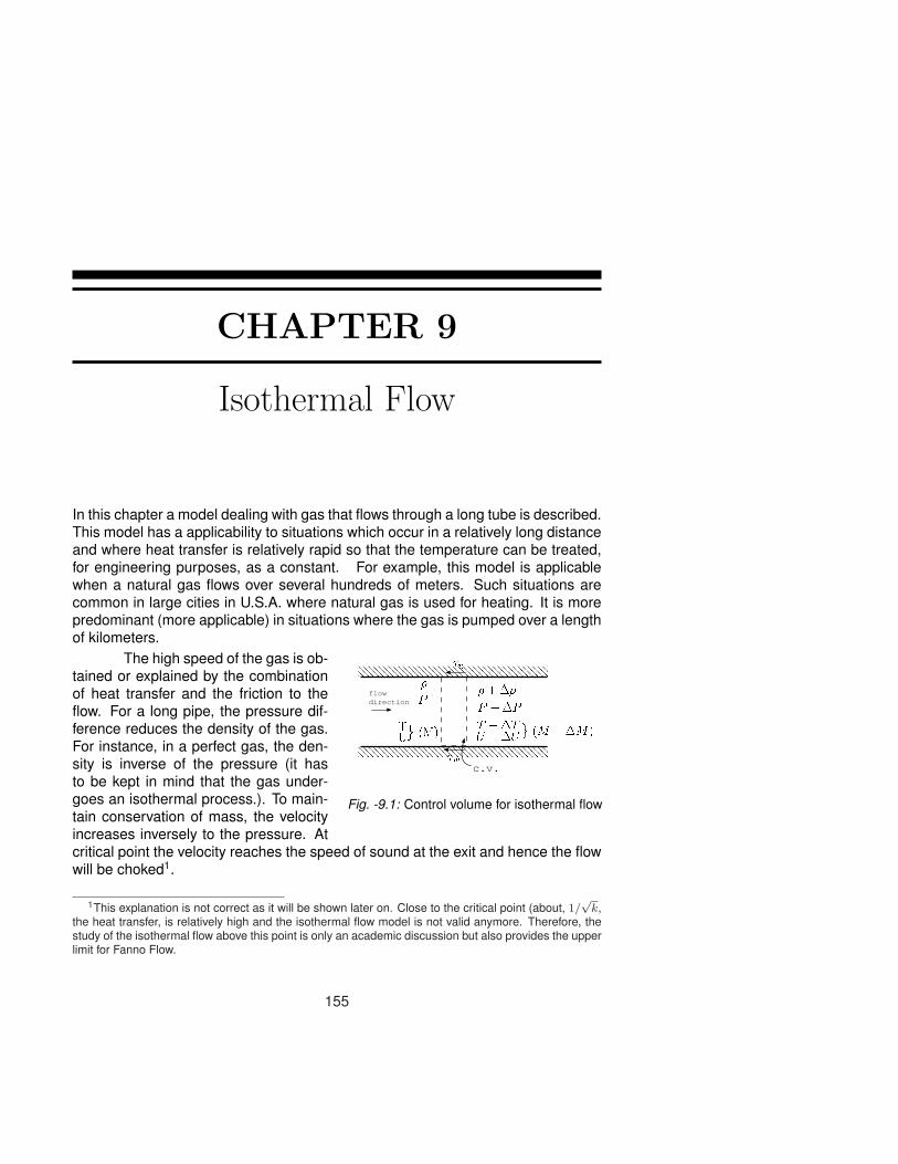
CHAPTER 9
Isothermal Flow
In this chapter a model dealing with gas that flows through a long tube is described.This model has a applicability to situations which occur in a relatively long distanceand where heat transfer is relatively rapid so that the temperature can be treated,for engineering purposes, as a constant. For example, this model is applicablewhen a natural gas flows over several hundreds of meters. Such situations arecommon in large cities in U.S.A. where natural gas is used for heating. It is morepredominant (more applicable) in situations where the gas is pumped over a lengthof kilometers.
PTUg (M)� +��P +�Pc.v.
flowdirection
�T +�TU +�Ug (M + �M)
�w�w
Fig. -9.1: Control volume for isothermal flow
The high speed of the gas is ob-tained or explained by the combinationof heat transfer and the friction to theflow. For a long pipe, the pressure dif-ference reduces the density of the gas.For instance, in a perfect gas, the den-sity is inverse of the pressure (it hasto be kept in mind that the gas under-goes an isothermal process.). To main-tain conservation of mass, the velocityincreases inversely to the pressure. Atcritical point the velocity reaches the speed of sound at the exit and hence the flowwill be choked1.
1This explanation is not correct as it will be shown later on. Close to the critical point (about, 1/√
k,the heat transfer, is relatively high and the isothermal flow model is not valid anymore. Therefore, thestudy of the isothermal flow above this point is only an academic discussion but also provides the upperlimit for Fanno Flow.
155

156 CHAPTER 9. ISOTHERMAL FLOW
9.1 The Control Volume Analysis/Governing equationsFigure (9.1) describes the flow of gas from the left to the right. The heat transfer upstream (or down stream) is assumed to be negligible. Hence, the energy equationcan be written as the following:
dQ
m= cpdT + d
U2
2= cpdT0 (9.1)
The momentum equation is written as the following
−AdP − τwdAwetted area = mdU (9.2)
where A is the cross section area (it doesn’t have to be a perfect circle; a closeenough shape is sufficient.). The shear stress is the force per area that acts onthe fluid by the tube wall. The Awetted area is the area that shear stress acts on.The second law of thermodynamics reads
s2 − s1
Cp= ln
T2
T1− k − 1
kln
P2
P1(9.3)
The mass conservation is reduced to
m = constant = ρUA (9.4)
Again it is assumed that the gas is a perfect gas and therefore, equation ofstate is expressed as the following:
P = ρRT (9.5)
9.2 Dimensionless RepresentationIn this section the equations are transformed into the dimensionless form and pre-sented as such. First it must be recalled that the temperature is constant andtherefore, equation of state reads
dP
P=
dρ
ρ(9.6)
It is convenient to define a hydraulic diameter
DH =4× Cross Section Area
wetted perimeter(9.7)

9.2. DIMENSIONLESS REPRESENTATION 157
Now, the Fanning friction factor2 is introduced, this factor is a dimensionlessfriction factor sometimes referred to as the friction coefficient as
f =τw
12ρU2
(9.8)
Substituting equation (9.8) into momentum equation (9.2) yields
−dP − 4dx
DHf
(12ρU2
)=
mA︷︸︸︷
ρU dU (9.9)
Rearranging equation (9.9) and using the identify for perfect gas M2 = ρU2/kPyields:
−dP
P− 4fdx
DH
(kPM2
2
)=
kPM2dU
U(9.10)
Now the pressure, P as a function of the Mach number has to substitute alongwith velocity, U .
U2 = kRTM2 (9.11)
Differentiation of equation (9.11) yields
d(U2) = kR(M2 dT + T d(M2)
)(9.12)
d(M2)M2
=d(U2)U2
− dT
T(9.13)
Now it can be noticed that dT = 0 for isothermal process and therefore
d(M2)M2
=d(U2)U2
=2U dU
U2=
2dU
U(9.14)
The dimensionalization of the mass conservation equation yields
dρ
ρ+
dU
U=
dρ
ρ+
2UdU
2U2=
dρ
ρ+
d(U2)2 U2
= 0 (9.15)
Differentiation of the isotropic (stagnation) relationship of the pressure (5.11)yields
dP0
P0=
dP
P+
(12kM2
1 + k−12 M2
)dM2
M2(9.16)
2It should be noted that Fanning factor based on hydraulic radius, instead of diameter friction equa-tion, thus “Fanning f” values are only 1/4th of “Darcy f” values.

158 CHAPTER 9. ISOTHERMAL FLOW
Differentiation of equation (5.9) yields:
dT0 = dT
(1 +
k − 12
M2
)+ T
k − 12
dM2 (9.17)
Notice that dT0 6= 0 in an isothermal flow. There is no change in the actualtemperature of the flow but the stagnation temperature increases or decreasesdepending on the Mach number (supersonic flow of subsonic flow). Substituting Tfor equation (9.17) yields:
dT0 =T0
k−12 d M2
(1 + k−1
2 M2) M2
M2(9.18)
Rearranging equation (9.18) yields
dT0
T0=
(k − 1) M2
2(1 + k−1
2
) dM2
M2(9.19)
By utilizing the momentum equation it is possible to obtain a relation be-tween the pressure and density. Recalling that an isothermal flow (T = 0) andcombining it with perfect gas model yields
dP
P=
dρ
ρ(9.20)
From the continuity equation (see equation (9.14)) leads
dM2
M2=
2dU
U(9.21)
The four equations momentum, continuity (mass), energy, state are de-scribed above. There are 4 unknowns (M, T, P, ρ)3 and with these four equationsthe solution is attainable. One can notice that there are two possible solutions (be-cause of the square power). These different solutions are supersonic and subsonicsolution.
The distance friction, 4fLD , is selected as the choice for the independent
variable. Thus, the equations need to be obtained as a function of 4fLD . The
density is eliminated from equation (9.15) when combined with equation (9.20) tobecome
dP
P= −dU
U(9.22)
3Assuming the upstream variables are known.

9.2. DIMENSIONLESS REPRESENTATION 159
After substituting the velocity (9.22) into equation (9.10), one can obtain
−dP
P− 4fdx
DH
(kPM2
2
)= kPM2 dP
P(9.23)
Equation (9.23) can be rearranged into
dP
P=
dρ
ρ= −dU
U= −1
2dM2
M2= − kM2
2 (1− kM2)4f
dx
D(9.24)
Similarly or by other path the stagnation pressure can be expressed as a functionof 4fL
D
dP0
P0=
kM2(1− k+1
2 M2)
2 (kM2 − 1)(1 + k−1
2 M2)4f
dx
D(9.25)
dT0
T0=
k (1− k)M2
2 (1− kM2)(1 + k−1
2 M2)4f
dx
D(9.26)
The variables in equation (9.24) can be separated to obtain integrable form asfollows
∫ L
0
4fdx
D=
∫ 1/k
M2
1− kM2kM2
dM2 (9.27)
It can be noticed that at the entrance (x = 0) for which M = Mx=0 (the initialvelocity in the tube isn’t zero). The term 4fL
D is positive for any x, thus, the term onthe other side has to be positive as well. To obtain this restriction 1 = kM2. Thus,the value M = 1√
kis the limiting case from a mathematical point of view. When
Mach number larger than M > 1√k
it makes the right hand side of the integratenegative. The physical meaning of this value is similar to M = 1 choked flow whichwas discussed in a variable area flow in Chapter (5).
Further it can be noticed from equation (9.26) that when M → 1√k
the valueof right hand side approaches infinity (∞). Since the stagnation temperature (T0)has a finite value which means that dT0 → ∞. Heat transfer has a limited valuetherefore the model of the flow must be changed. A more appropriate model is anadiabatic flow model yet it can serve as a bounding boundary (or limit).
Integration of equation (9.27) requires information about the relationshipbetween the length, x, and friction factor f . The friction is a function of theReynolds number along the tube. Knowing the Reynolds number variations isimportant. The Reynolds number is defined as
Re =D U ρ
µ(9.28)

160 CHAPTER 9. ISOTHERMAL FLOW
The quantity U ρ is constant along the tube (mass conservation) under constantarea. Thus, the only viscosity is varied along the tube. However under the assump-tion of ideal gas, viscosity is only a function of the temperature. The temperaturein isothermal process (the definition) is constant and thus the viscosity is constant.In real gas the pressure effect is very minimal as described in “Basic of fluid me-chanics” by this author. Thus, the friction factor can be integrated to yield
4fL
D
∣∣∣∣max
=1− kM2
kM2+ ln kM2 (9.29)
The definition for perfect gas yields M2 = U2/kRT and noticing thatT = constant is used to describe the relation of the properties at M = 1/
√k.
By denoting the superscript symbol ∗ for the choking condition, one can obtain that
M2
U2=
1/k
U∗2 (9.30)
Rearranging equation (9.30) is transformed intoU
U∗ =√
kM (9.31)
Utilizing the continuity equation provides
ρU = ρ∗U∗; =⇒ ρ
ρ∗=
1√kM
(9.32)
Reusing the perfect–gas relationship
P
P ∗=
ρ
ρ∗=
1√kM (9.33)
Now utilizing the relation for stagnated isotropic pressure one can obtain
P0
P ∗0=
P
P ∗
[1 + k−1
2 M2
1 + k−12k
] kk−1
(9.34)
Substituting for PP∗ equation (9.33) and rearranging yields
P0
P ∗0=
1√k
(2k
3k − 1
) kk−1
(1 +
k − 12
M2
) kk−1 1
M (9.35)
And the stagnation temperature at the critical point can be expressed as
T0
T ∗0=
T
T ∗1 + k−1
2 M2
1 + k−12k
=2k
3k − 1
(1 +
k − 12
)M2
(9.36)
These equations (9.31)-(9.36) are presented on in Figure (9.2)

9.3. THE ENTRANCE LIMITATION OF SUPERSONIC BRANCH 161
0.1 1 10Mach number
0.01
0.1
1
1e+01
1e+024fL
D
or P
P*
ρρ∗
T0/T
0
*
P0/P
0
*
Isothermal Flow
P/P*, ρ/ρ*
and T0/T
0
* as a function of M
Fri Feb 18 17:23:43 2005
Fig. -9.2: Description of the pressure, temperature relationships as a function of the Machnumber for isothermal flow
9.3 The Entrance Limitation of Supersonic BranchSituations where the conditions at the tube exit have not arrived at the critical con-ditions are discussed here. It is very useful to obtain the relationship between theentrance and the exit condition for this case. Denote 1 and 2 as the conditions atthe inlet and exit respectably. From equation (9.24)
4fL
D=
4fL
D
∣∣∣∣max1
− 4fL
D
∣∣∣∣max2
=1− kM1
2
kM12 − 1− kM2
2
kM22 + ln
(M1
M2
)2
(9.37)
For the case that M1 >> M2 and M1 → 1 equation (9.37) is reduced into thefollowing approximation
4fL
D= 2 ln M1 − 1−
∼0︷ ︸︸ ︷1− kM2
2
kM22 (9.38)

162 CHAPTER 9. ISOTHERMAL FLOW
Solving for M1 results in
M1 ∼e 12 ( 4fL
D +1)(9.39)
This relationship shows the maximum limit that Mach number can approach whenthe heat transfer is extraordinarily fast. In reality, even small 4fL
D > 2 results ina Mach number which is larger than 4.5. This velocity requires a large entrancelength to achieve good heat transfer. With this conflicting mechanism obviously theflow is closer to the Fanno flow model. Yet this model provides the directions of theheat transfer effects on the flow.
9.4 Comparison with Incompressible FlowThe Mach number of the flow in some instances is relatively small. In these cases,one should expect that the isothermal flow should have similar characteristics asincompressible flow. For incompressible flow, the pressure loss is expressed asfollows
P1 − P2 =4fL
D
U2
2(9.40)
Now note that for incompressible flow U1 = U2 = U and 4fLD represent the ratio of
the traditional h12. To obtain a similar expression for isothermal flow, a relationshipbetween M2 and M1 and pressures has to be derived. From equation (9.40) onecan obtained that
M2 = M1P1
P2(9.41)
Substituting this expression into (9.41) yields
4fL
D=
1kM1
2
(1−
(P2
P1
)2)− ln
(P2
P1
)2
(9.42)
Because f is always positive there is only one solution to the above equation eventhough M2.
Expanding the solution for small pressure ratio drop, P1 − P2/P1, by somemathematics.
denote
χ =P1 − P2
P1(9.43)
Now equation (9.42) can be transformed into
4fL
D=
1kM1
2
(1−
(P2 − P1 + P1
P1
)2)− ln
(1P2P1
)2
(9.44)

9.4. COMPARISON WITH INCOMPRESSIBLE FLOW 163
4fL
D=
1kM1
2
(1− (1− χ)2
)− ln
(1
1− χ
)2
(9.45)
4fL
D=
1kM1
2
(2χ− χ2
)− ln(
11− χ
)2
(9.46)
now we have to expand into a series around χ = 0 and remember that
f(x) = f(0) + f ′(0)x + f ′′(0)x2
2+ 0
(x3
)(9.47)
and for example the first derivative of
d
dχln
(1
1− χ
)2∣∣∣∣∣χ=0
=
(1− χ)2 × [(−2)(1− χ)−3
](−1)
∣∣∣χ=0
= 2 (9.48)
similarly it can be shown that f ′′(χ = 0) = 1 equation (9.46) now can beapproximated as
4fL
D=
1kM1
2 (2χ− χ2)− (2χ− χ2
)+ f
(χ3
)(9.49)
rearranging equation (9.49) yields
4fL
D=
χ
kM12
[(2− χ)− kM1
2 (2− χ)]+ f
(χ3
)(9.50)
and further rearrangement yields
4fL
D=
χ
kM12
[2(1− kM1
2)− (1 + kM1
2)χ]+ f
(χ3
)(9.51)
in cases that χ is small
4fL
D≈ χ
kM12
[2(1− kM1
2)− (1 + kM1
2)χ]
(9.52)
The pressure difference can be plotted as a function of the M1 for givenvalue of 4fL
D . Equation (9.52) can be solved explicitly to produce a solution for
χ =1− kM1
2
1 + kM12 −
√1− kM1
2
1 + kM12 −
kM12
1 + kM12
4fL
D(9.53)
A few observations can be made about equation (9.53).

164 CHAPTER 9. ISOTHERMAL FLOW
9.5 Supersonic BranchApparently, this analysis/model is over simplified for the supersonic branch anddoes not produce reasonable results since it neglects to take into account the heattransfer effects. A dimensionless analysis4 demonstrates that all the common ma-terials that the author is familiar which creates a large error in the fundamentalassumption of the model and the model breaks. Nevertheless, this model can pro-vide a better understanding to the trends and deviations of the Fanno flow model.
In the supersonic flow, the hydraulic entry length is very large as will beshown below. However, the feeding diverging nozzle somewhat reduces the re-quired entry length (as opposed to converging feeding). The thermal entry lengthis in the order of the hydrodynamic entry length (look at the Prandtl number, (0.7-1.0), value for the common gases.). Most of the heat transfer is hampered in thesublayer thus the core assumption of isothermal flow (not enough heat transfer sothe temperature isn’t constant) breaks down5.
The flow speed at the entrance is very large, over hundred of meters persecond. For example, a gas flows in a tube with 4fL
D = 10 the required entry Machnumber is over 200. Almost all the perfect gas model substances dealt with inthis book, the speed of sound is a function of temperature. For this illustration,for most gas cases the speed of sound is about 300[m/sec]. For example, evenwith low temperature like 200K the speed of sound of air is 283[m/sec]. So, evenfor relatively small tubes with 4fL
D = 10 the inlet speed is over 56 [km/sec]. Thisrequires that the entrance length to be larger than the actual length of the tub forair. Remember from Fluid Dynamic book
Lentrance = 0.06UD
ν(9.54)
The typical values of the the kinetic viscosity, ν, are 0.0000185 kg/m-sec at 300Kand 0.0000130034 kg/m-sec at 200K. Combine this information with our case of4fLD = 10
Lentrance
D= 250746268.7
On the other hand a typical value of friction coefficient f = 0.005 results in
Lmax
D=
104× 0.005
= 500
The fact that the actual tube length is only less than 1% of the entry length meansthat the assumption is that the isothermal flow also breaks (as in a large responsetime).
Now, if Mach number is changing from 10 to 1 the kinetic energy change isabout T0
T0∗ = 18.37 which means that the maximum amount of energy is insufficient.
4This dimensional analysis is a bit tricky, and is based on estimates. Currently and ashamedly theauthor is looking for a more simplified explanation. The current explanation is correct but based onhands waving and definitely does not satisfy the author.
5see Kays and Crawford “Convective Heat Transfer” (equation 12-12).

9.7. ISOTHERMAL FLOW EXAMPLES 165
Now with limitation, this topic will be covered in the next version because itprovide some insight and boundary to the Fanno Flow model.
9.6 Figures and Tables
Table -9.1: The Isothermal Flow basic parameters
M 4fLD
PP∗
P0
P0∗
ρρ∗
T0
T0∗
0.03000 785.97 28.1718 17.6651 28.1718 0.875160.04000 439.33 21.1289 13.2553 21.1289 0.875280.05000 279.06 16.9031 10.6109 16.9031 0.875440.06000 192.12 14.0859 8.8493 14.0859 0.875630.07000 139.79 12.0736 7.5920 12.0736 0.875860.08000 105.89 10.5644 6.6500 10.5644 0.876120.09000 82.7040 9.3906 5.9181 9.3906 0.876420.10000 66.1599 8.4515 5.3334 8.4515 0.876750.20000 13.9747 4.2258 2.7230 4.2258 0.882000.25000 7.9925 3.3806 2.2126 3.3806 0.885940.30000 4.8650 2.8172 1.8791 2.8172 0.890750.35000 3.0677 2.4147 1.6470 2.4147 0.896440.40000 1.9682 2.1129 1.4784 2.1129 0.903000.45000 1.2668 1.8781 1.3524 1.8781 0.910440.50000 0.80732 1.6903 1.2565 1.6903 0.918750.55000 0.50207 1.5366 1.1827 1.5366 0.927940.60000 0.29895 1.4086 1.1259 1.4086 0.938000.65000 0.16552 1.3002 1.0823 1.3002 0.948940.70000 0.08085 1.2074 1.0495 1.2074 0.960750.75000 0.03095 1.1269 1.0255 1.1269 0.973440.80000 0.00626 1.056 1.009 1.056 0.987000.81000 0.00371 1.043 1.007 1.043 0.989820.81879 0.00205 1.032 1.005 1.032 0.992320.82758 0.000896 1.021 1.003 1.021 0.994850.83637 0.000220 1.011 1.001 1.011 0.997410.84515 0.0 1.000 1.000 1.000 1.000
9.7 Isothermal Flow ExamplesThere can be several kinds of questions aside from the proof questions6 Generally,the “engineering” or practical questions can be divided into driving force (pressure
6The proof questions are questions that ask for proof or for finding a mathematical identity (normallygood for mathematicians and study of perturbation methods). These questions or examples will appearin the later versions.

166 CHAPTER 9. ISOTHERMAL FLOW
difference), resistance (diameter, friction factor, friction coefficient, etc.), and massflow rate questions. In this model no questions about shock (should) exist7.
The driving force questions deal with what should be the pressure differ-ence to obtain certain flow rate. Here is an example.
Example 9.1:A tube of 0.25 [m] diameter and 5000 [m] in length is attached to a pump. Whatshould be the pump pressure so that a flow rate of 2 [kg/sec] will be achieved?Assume that friction factor f = 0.005 and the exit pressure is 1[bar]. The specificheat for the gas, k = 1.31, surroundings temperature 27◦C, R = 290
[J
Kkg
]. Hint:
calculate the maximum flow rate and then check if this request is reasonable.
SOLUTIONIf the flow was incompressible then for known density, ρ, the velocity can be calcu-lated by utilizing ∆P = 4fL
DU2
2g . In incompressible flow, the density is a function ofthe entrance Mach number. The exit Mach number is not necessarily 1/
√k i.e. the
flow is not choked. First, check whether flow is choked (or even possible).Calculating the resistance, 4fL
D
4fL
D=
4× 0.00550000.25
= 400
Utilizing Table (9.1) or the program provides
M 4fLD
PP∗
P0
P0∗
ρρ∗
T0
T0∗
0.04331 400.00 20.1743 12.5921 0.0 0.89446
The maximum flow rate (the limiting case) can be calculated by utilizing theabove table. The velocity of the gas at the entrance U = cM = 0.04331 ×√
1.31× 290× 300 ∼= 14.62[
msec
]. The density reads
ρ =P
RT=
2, 017, 450290× 300
∼= 23.19[
kg
m3
]
The maximum flow rate then reads
m = ρAU = 23.19× π × (0.25)2
4× 14.62 ∼= 16.9
[kg
sec
]
The maximum flow rate is larger then the requested mass rate hence the flow isnot choked. It is note worthy to mention that since the isothermal model breaksaround the choking point, the flow rate is really some what different. It is moreappropriate to assume an isothermal model hence our model is appropriate.
7Those who are mathematically inclined can include these kinds of questions but there are no realworld applications to isothermal model with shock.

9.7. ISOTHERMAL FLOW EXAMPLES 167
To solve this problem the flow rate has to be calculated as
m = ρAU = 2.0[
kg
sec
]
m =P1
RTA
kU
k=
P1√kRT
AkU√kRT
=P1
cAkM1
Now combining with equation (9.41) yields
m =M2P2Ak
c
M2 =mc
P2Ak=
2× 337.59
100000× π×(0.25)2
4 × 1.31= 0.103
From Table (9.1) or by utilizing the program
M 4fLD
PP∗
P0
P0∗
ρρ∗
T0
T0∗
0.10300 66.6779 8.4826 5.3249 0.0 0.89567
The entrance Mach number is obtained by
4fL
D
∣∣∣∣1
= 66.6779 + 400 ∼= 466.68
M 4fLD
PP∗
P0
P0∗
ρρ∗
T0
T0∗
0.04014 466.68 21.7678 13.5844 0.0 0.89442
The pressure should be
P = 21.76780× 8.4826 = 2.566[bar]
Note that tables in this example are for k = 1.31
Example 9.2:A flow of gas was considered for a distance of 0.5 [km] (500 [m]). A flow rate of0.2 [kg/sec] is required. Due to safety concerns, the maximum pressure allowedfor the gas is only 10[bar]. Assume that the flow is isothermal and k=1.4, calculatethe required diameter of tube. The friction coefficient for the tube can be assumedas 0.02 (A relative smooth tube of cast iron.). Note that tubes are provided inincrements of 0.5 [in]8. You can assume that the soundings temperature to be27◦C.
8It is unfortunate, but it seems that this standard will be around in USA for some time.

168 CHAPTER 9. ISOTHERMAL FLOW
SOLUTIONAt first, the minimum diameter will be obtained when the flow is choked. Thus,the maximum M1 that can be obtained when the M2 is at its maximum and backpressure is at the atmospheric pressure.
M1 = M2P2
P1=
Mmax︷︸︸︷1√k
110
= 0.0845
Now, with the value of M1 either by utilizing Table (9.1) or using the provided pro-gram yields
M 4fLD
PP∗
P0
P0∗
ρρ∗
T0
T0∗
0.08450 94.4310 10.0018 6.2991 0.0 0.87625
With 4fLD
∣∣∣max
= 94.431 the value of minimum diameter.
D =4fL
4fLD
∣∣∣max
' 4× 0.02× 50094.43
' 0.42359[m] = 16.68[in]
However, the pipes are provided only in 0.5 increments and the next size is 17[in]or 0.4318[m]. With this pipe size the calculations are to be repeated in reverse andproduces: (Clearly the maximum mass is determined with)
m = ρAU = ρAMc =P
RTAM
√kRT =
PAM√
k√RT
The usage of the above equation clearly applied to the whole pipe. The only pointthat must be emphasized is that all properties (like Mach number, pressure andetc) have to be taken at the same point. The new 4fL
D is
4fL
D=
4× 0.02× 5000.4318
' 92.64
M 4fLD
PP∗
P0
P0∗
ρρ∗
T0
T0∗
0.08527 92.6400 9.9110 6.2424 0.0 0.87627
To check whether the flow rate satisfies the requirement
m =106 × π×0.43182
4 × 0.0853×√1.4√287× 300
≈ 50.3[kg/sec]
Since 50.3 ≥ 0.2 the mass flow rate requirement is satisfied.

9.7. ISOTHERMAL FLOW EXAMPLES 169
It should be noted that P should be replaced by P0 in the calculations. The speedof sound at the entrance is
c =√
kRT =√
1.4× 287× 300 ∼= 347.2[ m
sec
]
and the density is
ρ =P
RT=
1, 000, 000287× 300
= 11.61[
kg
m3
]
The velocity at the entrance should be
U = M ∗ c = 0.08528× 347.2 ∼= 29.6[ m
sec
]
The diameter should be
D =
√4m
πUρ=
√4× 0.2
π × 29.6× 11.61∼= 0.027
Nevertheless, for the sake of the exercise the other parameters will be calculated.This situation is reversed question. The flow rate is given with the diameter of thepipe. It should be noted that the flow isn’t choked.
Example 9.3:A gas flows of from a station (a) with pressure of 20[bar] through a pipe with 0.4[m]diameter and 4000 [m] length to a different station (b). The pressure at the exit(station (b)) is 2[bar]. The gas and the sounding temperature can be assumedto be 300 K. Assume that the flow is isothermal, k=1.4, and the average frictionf=0.01. Calculate the Mach number at the entrance to pipe and the flow rate.
SOLUTIONFirst, the information whether the flow is choked needs to be found. Therefore, atfirst it will be assumed that the whole length is the maximum length.
4fL
D
∣∣∣∣max
=4× 0.01× 4000
0.4= 400
with 4fLD
∣∣∣max
= 400 the following can be written
M 4fLD
T0
T0∗T
ρρ∗T
PP∗T
P0
P0∗T
0.0419 400.72021 0.87531 20.19235 20.19235 12.66915
From the table M1 ≈ 0.0419 ,and P0P0∗T ≈ 12.67
P0∗T ∼= 28
12.67' 2.21[bar]

170 CHAPTER 9. ISOTHERMAL FLOW
The pressure at point (b) by utilizing the isentropic relationship (M = 1) pressureratio is 0.52828.
P2 =P0∗T
(P2
P0∗T
) = 2.21× 0.52828 = 1.17[bar]
As the pressure at point (b) is smaller than the actual pressure P ∗ < P2 than theactual pressure one must conclude that the flow is not choked. The solution is aniterative process.
1. guess reasonable value of M1 and calculate 4fLD
2. Calculate the value of 4fLD
∣∣∣2
by subtracting 4fLD
∣∣∣1− 4fL
D
3. Obtain M2 from the Table ? or by using the Potto–GDC.
4. Calculate the pressure, P2 bear in mind that this isn’t the real pressure butbased on the assumption.
5. Compare the results of guessed pressure P2 with the actual pressure andchoose new Mach number M1 accordingly.
Now the process has been done for you and is provided in figure ??? or in thetable obtained from the provided program.
M1 M24fLD
∣∣max
∣∣1
4fLD
P2
P1
0.0419 0.59338 400.32131 400.00000 0.10000
The flow rate is
m = ρAMc =P√
k√RT
π ×D2
4M =
2000000√
1.4√300× 287
π × 0.22 × 0.0419
' 42.46[kg/sec]
In this chapter, there are no examples on isothermal with supersonic flow.
9.8 Unchoked situations in Fanno Flow
Table -9.2: The flow parameters for unchoked flow
M1 M24fLD
∣∣max
∣∣1
4fLD
P2
P1
0.7272 0.84095 0.05005 0.05000 0.100000.6934 0.83997 0.08978 0.08971 0.10000
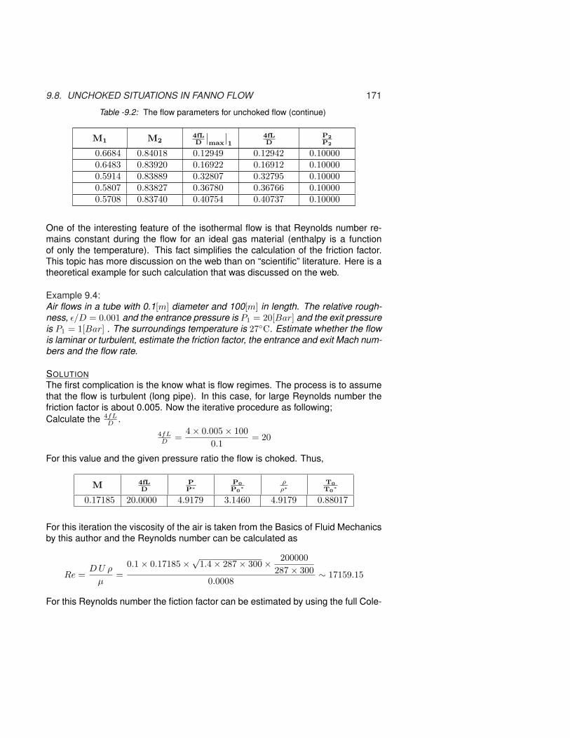
9.8. UNCHOKED SITUATIONS IN FANNO FLOW 171
Table -9.2: The flow parameters for unchoked flow (continue)
M1 M24fLD
∣∣max
∣∣1
4fLD
P2
P2
0.6684 0.84018 0.12949 0.12942 0.100000.6483 0.83920 0.16922 0.16912 0.100000.5914 0.83889 0.32807 0.32795 0.100000.5807 0.83827 0.36780 0.36766 0.100000.5708 0.83740 0.40754 0.40737 0.10000
One of the interesting feature of the isothermal flow is that Reynolds number re-mains constant during the flow for an ideal gas material (enthalpy is a functionof only the temperature). This fact simplifies the calculation of the friction factor.This topic has more discussion on the web than on “scientific” literature. Here is atheoretical example for such calculation that was discussed on the web.
Example 9.4:Air flows in a tube with 0.1[m] diameter and 100[m] in length. The relative rough-ness, ε/D = 0.001 and the entrance pressure is P1 = 20[Bar] and the exit pressureis P1 = 1[Bar] . The surroundings temperature is 27◦C. Estimate whether the flowis laminar or turbulent, estimate the friction factor, the entrance and exit Mach num-bers and the flow rate.
SOLUTIONThe first complication is the know what is flow regimes. The process is to assumethat the flow is turbulent (long pipe). In this case, for large Reynolds number thefriction factor is about 0.005. Now the iterative procedure as following;Calculate the 4fL
D .4fLD =
4× 0.005× 1000.1
= 20
For this value and the given pressure ratio the flow is choked. Thus,
M 4fLD
PP∗
P0
P0∗
ρρ∗
T0
T0∗
0.17185 20.0000 4.9179 3.1460 4.9179 0.88017
For this iteration the viscosity of the air is taken from the Basics of Fluid Mechanicsby this author and the Reynolds number can be calculated as
Re =D U ρ
µ=
0.1× 0.17185×√1.4× 287× 300× 200000287× 300
0.0008∼ 17159.15
For this Reynolds number the fiction factor can be estimated by using the full Cole-

172 CHAPTER 9. ISOTHERMAL FLOW
0 10 20 30 40 50 60 70 80 90 100
4fLD
0
0.1
0.2
0.3
0.4
0.5
0.6
0.7
0.8
0.9
1
M1
P2 / P
1 = 0.8
P2 / P
1 = 0.5
P2 / P
1 = 0.2
P2 / P
1 = 0.10
M1 isothermal flow
Fri Feb 25 17:20:14 2005
Fig. -9.3: The Mach number at the entrance to a tube under isothermal flow model as afunction 4fL
D
brook’s equation
1√f
= −2 log10
(ε/Dh
3.7+
2.51Re√
f
)(9.55)
or the approximated Haaland’s equation
1√f
= −1.8 log10
[(ε/D
3.7
)1.11
+6.9Re
](9.56)
which provide f = 0.0053 and it is a reasonable answer in one iteration. Repeatingthe iteration results in
4fLD =
4× 0.0053× 1000.1
= 21.2
with
M 4fLD
PP∗
P0
P0∗
ρρ∗
T0
T0∗
0.16689 21.4000 5.0640 3.2357 5.0640 0.87987

9.8. UNCHOKED SITUATIONS IN FANNO FLOW 173
And the “improved” Reynolds number is
Re =0.1× 0.16689×√1.4× 287× 300× 200000
287× 3000.0008
∼ 16669.6
And the friction number is .0054 which very good estimate compare with the as-sumption that this model was built on.
End Solution

174 CHAPTER 9. ISOTHERMAL FLOW
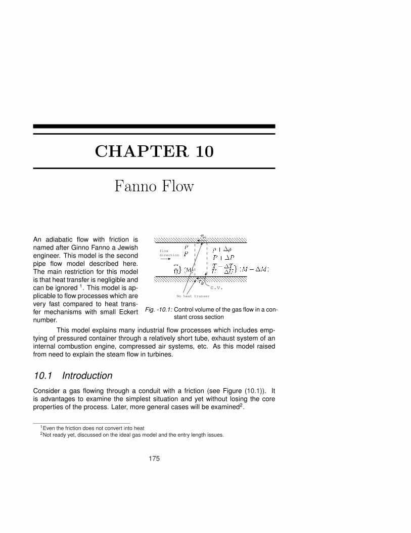
CHAPTER 10
Fanno Flow
PTUg (M)� +��P +�Pc.v.
flowdirection
�T +�TU +�Ug (M + �M)
�w�w
No heat transer
Fig. -10.1: Control volume of the gas flow in a con-stant cross section
An adiabatic flow with friction isnamed after Ginno Fanno a Jewishengineer. This model is the secondpipe flow model described here.The main restriction for this modelis that heat transfer is negligible andcan be ignored 1. This model is ap-plicable to flow processes which arevery fast compared to heat trans-fer mechanisms with small Eckertnumber.
This model explains many industrial flow processes which includes emp-tying of pressured container through a relatively short tube, exhaust system of aninternal combustion engine, compressed air systems, etc. As this model raisedfrom need to explain the steam flow in turbines.
10.1 IntroductionConsider a gas flowing through a conduit with a friction (see Figure (10.1)). Itis advantages to examine the simplest situation and yet without losing the coreproperties of the process. Later, more general cases will be examined2.
1Even the friction does not convert into heat2Not ready yet, discussed on the ideal gas model and the entry length issues.
175

176 CHAPTER 10. FANNO FLOW
10.2 Fanno ModelThe mass (continuity equation) balance can be written as
m = ρAU = constant (10.1)↪→ ρ1U1 = ρ2U2
The energy conservation (under the assumption that this model is adia-batic flow and the friction is not transformed into thermal energy) reads
T01 = T02 (10.2)
↪→ T1 +U1
2
2cp= T2 +
U22
2cp
(10.3)
Or in a derivative form
CpdT + d
(U2
2
)= 0 (10.4)
Again for simplicity, the perfect gas model is assumed3.
P = ρRT (10.5)
↪→ P1
ρ1T1=
P2
ρ2T2
It is assumed that the flow can be approximated as one–dimensional. Theforce acting on the gas is the friction at the wall and the momentum conservationreads
−AdP − τwdAw = mdU (10.6)
It is convenient to define a hydraulic diameter as
DH =4× Cross Section Area
wetted perimeter(10.7)
Or in other words
A =πDH
2
4(10.8)
3The equation of state is written again here so that all the relevant equations can be found when thischapter is printed separately.

10.3. NON–DIMENSIONALIZATION OF THE EQUATIONS 177
It is convenient to substitute D for DH and yet it still will be referred to the samename as the hydraulic diameter. The infinitesimal area that shear stress is actingon is
dAw = πDdx (10.9)
Introducing the Fanning friction factor as a dimensionless friction factor which issome times referred to as the friction coefficient and reads as the following:
f =τw
12ρU2
(10.10)
By utilizing equation (10.2) and substituting equation (10.10) into momentumequation (10.6) yields
−
A︷ ︸︸ ︷πD2
4dP − πDdx
τw︷ ︸︸ ︷f
(12ρU2
)= A
mA︷︸︸︷
ρU dU (10.11)
Dividing equation (10.11) by the cross section area, A and rearrangingyields
−dP +4fdx
D
(12ρU2
)= ρUdU (10.12)
The second law is the last equation to be utilized to determine the flow direction.
s2 ≥ s1 (10.13)
10.3 Non–Dimensionalization of the EquationsBefore solving the above equation a dimensionless process is applied. By utilizingthe definition of the sound speed to produce the following identities for perfect gas
M2 =(
U
c
)2
=U2
k RT︸︷︷︸Pρ
(10.14)
Utilizing the definition of the perfect gas results in
M2 =ρU2
kP(10.15)

178 CHAPTER 10. FANNO FLOW
Using the identity in equation (10.14) and substituting it into equation (10.11) andafter some rearrangement yields
−dP +4fdx
DH
(12kPM2
)=
ρU2
UdU =
ρU2
︷ ︸︸ ︷kPM2 dU
U(10.16)
By further rearranging equation (10.16) results in
−dP
P− 4fdx
D
(kM2
2
)= kM2 dU
U(10.17)
It is convenient to relate expressions of (dP/P ) and dU/U in terms of the Machnumber and substituting it into equation (10.17). Derivative of mass conservation((10.2)) results in
dρ
ρ+
dUU︷ ︸︸ ︷
12
dU2
U2= 0 (10.18)
The derivation of the equation of state (10.5) and dividing the results by equationof state (10.5) results
dP
P=
dρ
ρ+
dT
dT(10.19)
Derivation of the Mach identity equation (10.14) and dividing by equation (10.14)yields
d(M2)M2
=d(U2)U2
− dT
T(10.20)
Dividing the energy equation (10.4) by Cp and by utilizing the definition Machnumber yields
dT
T+
1(kR
(k − 1)
)
︸ ︷︷ ︸Cp
1T
U2
U2d
(U2
2
)=
↪→ dT
T+
(k − 1)kRT︸︷︷︸
c2
U2
U2d
(U2
2
)=
↪→ dT
T+
k − 12
M2 dU2
U2= 0 (10.21)
Equations (10.17), (10.18), (10.19), (10.20), and (10.21) need to be solved. Theseequations are separable so one variable is a function of only single variable (the

10.3. NON–DIMENSIONALIZATION OF THE EQUATIONS 179
chosen as the independent variable). Explicit explanation is provided for only twovariables, the rest variables can be done in a similar fashion. The dimensionlessfriction, 4fL
D , is chosen as the independent variable since the change in the dimen-sionless resistance, 4fL
D , causes the change in the other variables.Combining equations (10.19) and (10.21) when eliminating dT/T results
dP
P=
dρ
ρ− (k − 1)M2
2dU2
U2(10.22)
The term dρρ can be eliminated by utilizing equation (10.18) and substituting it into
equation (10.22) and rearrangement yields
dP
P= −1 + (k − 1)M2
2dU2
U2(10.23)
The term dU2/U2 can be eliminated by using (10.23)
dP
P= −kM2
(1 + (k − 1)M2
)
2(1−M2)4fdx
D(10.24)
The second equation for Mach number, M variable is obtained by combining equa-tion (10.20) and (10.21) by eliminating dT/T . Then dρ/ρ and U are eliminated byutilizing equation (10.18) and equation (10.22). The only variable that is left is P(or dP/P ) which can be eliminated by utilizing equation (10.24) and results in
4fdx
D=
(1−M2
)dM2
kM4(1 + k−12 M2)
(10.25)
Rearranging equation (10.25) results in
dM2
M2=
kM2(1 + k−1
2 M2)
1−M2
4fdx
D(10.26)
After similar mathematical manipulation one can get the relationship for thevelocity to read
dU
U=
kM2
2 (1−M2)4fdx
D(10.27)
and the relationship for the temperature is
dT
T=
12
dc
c= −k(k − 1)M4
2(1−M2)4fdx
D(10.28)
density is obtained by utilizing equations (10.27) and (10.18) to obtain
dρ
ρ= − kM2
2 (1−M2)4fdx
D(10.29)

180 CHAPTER 10. FANNO FLOW
The stagnation pressure is similarly obtained as
dP0
P0= −kM2
24fdx
D(10.30)
The second law reads
ds = Cp lndT
T−R ln
dP
P(10.31)
The stagnation temperature expresses as T0 = T (1 + (1 − k)/2M2). Takingderivative of this expression when M remains constant yields dT0 = dT (1 + (1 −k)/2M2) and thus when these equations are divided they yield
dT/T = dT0/T0 (10.32)
In similar fashion the relationship between the stagnation pressure and the pres-sure can be substituted into the entropy equation and result in
ds = Cp lndT0
T0−R ln
dP0
P0(10.33)
The first law requires that the stagnation temperature remains constant, (dT0 = 0).Therefore the entropy change is
ds
Cp= − (k − 1)
k
dP0
P0(10.34)
Using the equation for stagnation pressure the entropy equation yields
ds
Cp=
(k − 1)M2
24fdx
D(10.35)
10.4 The Mechanics and Why the Flow is Choked?The trends of the properties can be examined by looking in equations (10.24)through (10.34). For example, from equation (10.24) it can be observed that thecritical point is when M = 1. When M < 1 the pressure decreases downstreamas can be seen from equation (10.24) because fdx and M are positive. For thesame reasons, in the supersonic branch, M > 1, the pressure increases down-stream. This pressure increase is what makes compressible flow so different from“conventional” flow. Thus the discussion will be divided into two cases: One, flowabove speed of sound. Two, flow with speed below the speed of sound.

10.5. THE WORKING EQUATIONS 181
Why the flow is choked?
Here, the explanation is based on the equations developed earlier and there is noknown explanation that is based on the physics. First, it has to be recognized thatthe critical point is when M = 1. It will be shown that a change in location relative tothis point change the trend and it is singular point by itself. For example, dP (@M =1) = ∞ and mathematically it is a singular point (see equation (10.24)). Observingfrom equation (10.24) that increase or decrease from subsonic just below one M =(1 − ε) to above just above one M = (1 + ε) requires a change in a sign pressuredirection. However, the pressure has to be a monotonic function which means thatflow cannot crosses over the point of M = 1. This constrain means that becausethe flow cannot “crossover” M = 1 the gas has to reach to this speed, M = 1 atthe last point. This situation is called choked flow.
The Trends
The trends or whether the variables are increasing or decreasing can be observedfrom looking at the equation developed. For example, the pressure can be ex-amined by looking at equation (10.26). It demonstrates that the Mach numberincreases downstream when the flow is subsonic. On the other hand, when theflow is supersonic, the pressure decreases.
The summary of the properties changes on the sides of the branch
Subsonic SupersonicPressure, P decrease increaseMach number, M increase decreaseVelocity, U increase decreaseTemperature, T decrease increaseDensity, ρ decrease increaseStagnation Temperature, T0 decrease increase
10.5 The Working EquationsIntegration of equation (10.25) yields
4D
∫ Lmax
L
fdx =1k
1−M2
M2+
k + 12k
lnk+12 M2
1 + k−12 M2
(10.36)
A representative friction factor is defined as
f =1
Lmax
∫ Lmax
0
fdx (10.37)

182 CHAPTER 10. FANNO FLOW
In the isothermal flow model it was shown that friction factor is constant throughthe process if the fluid is ideal gas. Here, the Reynolds number defined in equation(9.28) is not constant because the temperature is not constant. The viscosity evenfor ideal gas is complex function of the temperature (further reading in “Basic ofFluid Mechanics” chapter one, Potto Project). However, the temperature variationis very limit. Simple improvement can be done by assuming constant constantviscosity (constant friction factor) and find the temperature on the two sides of thetube to improve the friction factor for the next iteration. The maximum error can beestimated by looking at the maximum change of the temperature. The temperaturecan be reduced by less than %20 for most range of the spesific heats ratio. Theviscosity change for this change is for many gases about 10%. For these gasesthe maximum increase of average Reynolds number is only 5%. What this changein Reynolds number does to friction factor? That depend in the range of Reynoldsnumber. For Reynolds number larger than 10,000 the change in friction factor canbe considered negligible. For the other extreme, laminar flow it can estimated thatchange of 5% in Reynolds number change about the same amount in friction factor.With the exception the jump from a laminar flow to a turbulent flow, the change isnoticeable but very small. In the light of the about discussion the friction factoris assumed to constant. By utilizing the mean average theorem equation (10.36)yields
4fLmax
D=
1k
1−M2
M2+
k + 12k
lnk+12 M2
1 + k−12 M2
(10.38)
It is common to replace the f with f which is adopted in this book.Equations (10.24), (10.27), (10.28), (10.29), (10.29), and (10.30) can be
solved. For example, the pressure as written in equation (10.23) is representedby 4fL
D , and Mach number. Now equation (10.24) can eliminate term 4fLD and
describe the pressure on the Mach number. Dividing equation (10.24) in equation(10.26) yields
dPP
dM2
M2
= − 1 + (k − 1M2
2M2(1 + k−1
2 M2)dM2 (10.39)
The symbol “*” denotes the state when the flow is choked and Mach number isequal to 1. Thus, M = 1 when P = P ∗ equation (10.39) can be integrated toyield:
P
P ∗=
1M
√k+12
1 + k−12 M2
(10.40)

10.5. THE WORKING EQUATIONS 183
In the same fashion the variables ratio can be obtained
T
T ∗=
c2
c∗2=
k+12
1 + k−12 M2
(10.41)
ρ
ρ∗=
1M
√1 + k−1
2 M2
k+12 (10.42)
U
U∗ =(
ρ
ρ∗
)−1
= M
√k+12
1 + k−12 M2
(10.43)
The stagnation pressure decreases and can be expressed by
P0
P0∗ =
(1+ 1−k2 M2)
kk−1
︷︸︸︷P0
PP
P0∗
P ∗︸︷︷︸( 2
k+1 )k
k−1
P ∗(10.44)
Using the pressure ratio in equation (10.40) and substituting it into equation(10.44) yields
P0
P0∗ =
(1 + k−1
2 M2
k+12
) kk−1 1
M
√1 + k−1
2 M2
k+12
(10.45)
And further rearranging equation (10.45) provides
P0
P0∗ =
1M
(1 + k−1
2 M2
k+12
) k+12(k−1)
(10.46)
The integration of equation (10.34) yields
s− s∗
cp= ln M2
√√√√(
k + 12M2
(1 + k−1
2 M2)) k+1
k
(10.47)

184 CHAPTER 10. FANNO FLOW
0.1 1 10Mach number
0.01
0.1
1
1e+01
1e+024fL
D
P
P*
T/T*
P0/P
0
*
U/U*
Fanno FlowP/P
*, ρ/ρ*
and T/T* as a function of M
Tue Sep 25 10:57:55 2007
Fig. -10.2: Various parameters in Fanno flow as a function of Mach number
The results of these equations are plotted in Figure (10.2) The Fanno flow is inmany cases shockless and therefore a relationship between two points should bederived. In most times, the “star” values are imaginary values that represent thevalue at choking. The real ratio can be obtained by two star ratios as an example
T2
T1=
TT∗
∣∣M2
TT∗
∣∣M1
(10.48)
A special interest is the equation for the dimensionless friction as following
∫ L2
L1
4fL
Ddx =
∫ Lmax
L1
4fL
Ddx−
∫ Lmax
L2
4fL
Ddx (10.49)
Hence,
(4fLmax
D
)
2
=(
4fLmax
D
)
1
− 4fL
D(10.50)
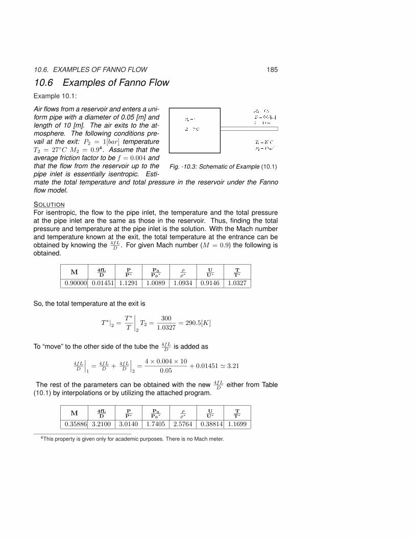
10.6. EXAMPLES OF FANNO FLOW 185
10.6 Examples of Fanno FlowExample 10.1:
D = 0:05[m℄P0 =?T0 =?ÆCP2 = 1[bar℄T2 = 27ÆC
M2 = 0:9L = 10[m℄
Fig. -10.3: Schematic of Example (10.1)
Air flows from a reservoir and enters a uni-form pipe with a diameter of 0.05 [m] andlength of 10 [m]. The air exits to the at-mosphere. The following conditions pre-vail at the exit: P2 = 1[bar] temperatureT2 = 27◦C M2 = 0.94. Assume that theaverage friction factor to be f = 0.004 andthat the flow from the reservoir up to thepipe inlet is essentially isentropic. Esti-mate the total temperature and total pressure in the reservoir under the Fannoflow model.
SOLUTIONFor isentropic, the flow to the pipe inlet, the temperature and the total pressureat the pipe inlet are the same as those in the reservoir. Thus, finding the totalpressure and temperature at the pipe inlet is the solution. With the Mach numberand temperature known at the exit, the total temperature at the entrance can beobtained by knowing the 4fL
D . For given Mach number (M = 0.9) the following isobtained.
M 4fLD
PP∗
P0
P0∗
ρρ∗
UU∗
TT∗
0.90000 0.01451 1.1291 1.0089 1.0934 0.9146 1.0327
So, the total temperature at the exit is
T ∗|2 =T ∗
T
∣∣∣∣2
T2 =300
1.0327= 290.5[K]
To “move” to the other side of the tube the 4fLD is added as
4fLD
∣∣∣1
= 4fLD + 4fL
D
∣∣∣2
=4× 0.004× 10
0.05+ 0.01451 ' 3.21
The rest of the parameters can be obtained with the new 4fLD either from Table
(10.1) by interpolations or by utilizing the attached program.
M 4fLD
PP∗
P0
P0∗
ρρ∗
UU∗
TT∗
0.35886 3.2100 3.0140 1.7405 2.5764 0.38814 1.1699
4This property is given only for academic purposes. There is no Mach meter.

186 CHAPTER 10. FANNO FLOW
Note that the subsonic branch is chosen. The stagnation ratios has to be addedfor M = 0.35886
M TT0
ρρ0
AA?
PP0
A×PA∗×P0
FF∗
0.35886 0.97489 0.93840 1.7405 0.91484 1.5922 0.78305
The total pressure P01 can be found from the combination of the ratios as follows:
P01 =
P1︷ ︸︸ ︷P∗︷ ︸︸ ︷
P2P ∗
P
∣∣∣∣2
P
P ∗
∣∣∣∣1
P0
P
∣∣∣∣1
=1× 11.12913
× 3.014× 10.915
= 2.91[Bar]
T01 =
T1︷ ︸︸ ︷T∗︷ ︸︸ ︷
T2T ∗
T
∣∣∣∣2
T
T ∗
∣∣∣∣1
T0
T
∣∣∣∣1
=300× 11.0327
× 1.17× 10.975
' 348K = 75◦C
Another academic question/example:
Example 10.2:
D = 0:025[m℄P0 = 29:65[bar℄T0 = 400K M1 = 3:0 L = 1:0[m℄shock
d-c nozzle
Mx =?atmosphereconditions
Fig. -10.4: The schematic of Example(10.2)
A system is composed of a convergent-divergent nozzle followed by a tube withlength of 2.5 [cm] in diameter and 1.0 [m]long. The system is supplied by a vessel.The vessel conditions are at 29.65 [Bar],400 K. With these conditions a pipe inletMach number is 3.0. A normal shock waveoccurs in the tube and the flow dischargesto the atmosphere, determine:
(a) the mass flow rate through the system;
(b) the temperature at the pipe exit; and
(c) determine the Mach number when a normal shock wave occurs [Mx].
Take k = 1.4, R = 287 [J/kgK] and f = 0.005.

10.6. EXAMPLES OF FANNO FLOW 187
SOLUTION
(a) Assuming that the pressure vessel is very much larger than the pipe, there-fore the velocity in the vessel can be assumed to be small enough so itcan be neglected. Thus, the stagnation conditions can be approximatedfor the condition in the tank. It is further assumed that the flow throughthe nozzle can be approximated as isentropic. Hence, T01 = 400K andP01 = 29.65[Par]
The mass flow rate through the system is constant and for simplicity point 1is chosen in which,
m = ρAMc
The density and speed of sound are unknowns and need to be computed.With the isentropic relationship the Mach number at point one (1) is known,then the following can be found either from Table (10.1) or the Potto–GDC
M TT0
ρρ0
AA?
PP0
A×PA∗×P0
FF∗
3.0000 0.35714 0.07623 4.2346 0.02722 0.11528 0.65326
The temperature is
T1 =T1
T01T01 = 0.357× 400 = 142.8K
Using the temperature, the speed of sound can be calculated as
c1 =√
kRT =√
1.4× 287× 142.8 ' 239.54[m/sec]
The pressure at point 1 can be calculated as
P1 =P1
P01P01 = 0.027× 30 ' 0.81[Bar]
The density as a function of other properties at point 1 is
ρ1 =P
RT
∣∣∣∣1
=8.1× 10⁴
287× 142.8' 1.97
[kg
m3
]
The mass flow rate can be evaluated from equation (10.2)
m = 1.97× π × 0.0252
4× 3× 239.54 = 0.69
[kg
sec
]

188 CHAPTER 10. FANNO FLOW
(b) First, check whether the flow is shockless by comparing the flow resistanceand the maximum possible resistance. From the Table (10.1) or by using thePotto–GDC, to obtain the following
M 4fLD
PP∗
P0
P0∗
ρρ∗
UU∗
TT∗
3.0000 0.52216 0.21822 4.2346 0.50918 1.9640 0.42857
and the conditions of the tube are
4fLD =
4× 0.005× 1.00.025
= 0.8
Since 0.8 > 0.52216 the flow is choked and with a shock wave.
The exit pressure determines the location of the shock, if a shock exists,by comparing “possible” Pexit to PB . Two possibilities are needed to bechecked; one, the shock at the entrance of the tube, and two, shock atthe exit and comparing the pressure ratios. First, the possibility that theshock wave occurs immediately at the entrance for which the ratio for Mx
are (shock wave Table (6.1))
Mx MyTy
Tx
ρy
ρx
Py
Px
P0y
P0x
3.0000 0.47519 2.6790 3.8571 10.3333 0.32834
After the shock wave the flow is subsonic with “M1”= 0.47519. (Fanno flowTable (10.1))
M 4fLD
PP∗
P0
P0∗
ρρ∗
UU∗
TT∗
0.47519 1.2919 2.2549 1.3904 1.9640 0.50917 1.1481
The stagnation values for M = 0.47519 are
M TT0
ρρ0
AA?
PP0
A×PA∗×P0
FF∗
0.47519 0.95679 0.89545 1.3904 0.85676 1.1912 0.65326

10.6. EXAMPLES OF FANNO FLOW 189
The ratio of exit pressure to the chamber total pressure is
P2
P0=
1︷ ︸︸ ︷(P2
P ∗
)(P ∗
P1
)(P1
P0y
)(P0y
P0x
)1︷ ︸︸ ︷(
P0x
P0
)
= 1× 12.2549
× 0.8568× 0.32834× 1
= 0.12476
The actual pressure ratio 1/29.65 = 0.0338 is smaller than the case in whichshock occurs at the entrance. Thus, the shock is somewhere downstream.One possible way to find the exit temperature, T2 is by finding the locationof the shock. To find the location of the shock ratio of the pressure ratio,P2P1
is needed. With the location of shock, “claiming” upstream from the exitthrough shock to the entrance. For example, calculate the parameters forshock location with known 4fL
D in the “y” side. Then either by utilizing shocktable or the program, to obtain the upstream Mach number.
The procedure for the calculations:
1)Calculate the entrance Mach number assuming the shock occurs at the exit:a) set M
′2 = 1 assume the flow in the entire tube is supersonic:
b) calculated M′1
Note this Mach number is the high Value.
2)
Calculate the entrance Mach assuming shock at the entrance.a) set M2 = 1b) add 4fL
D and calculated M1’ for subsonic branchc) calculated Mx for M1’Note this Mach number is the low Value.
3)
According your root finding algorithm5 calculate or guess the shock locationand then compute as above the new M1.a) set M2 = 1b) for the new 4fL
D and compute the new My ’ for the subsonic branchc) calculated Mx’ for the My ’d) Add the leftover of 4fL
D and calculated the M1
4) guess new location for the shock according to your finding root procedureand according to the result, repeat previous stage until the solution is ob-tained.
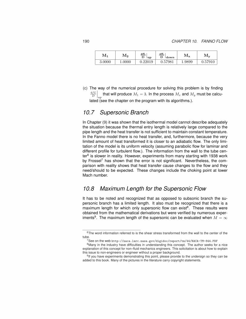
190 CHAPTER 10. FANNO FLOW
M1 M24fLD
∣∣up
4fLD
∣∣down
Mx My
3.0000 1.0000 0.22019 0.57981 1.9899 0.57910
(c) The way of the numerical procedure for solving this problem is by finding4fLD
∣∣∣up
that will produce M1 = 3. In the process Mx and My must be calcu-
lated (see the chapter on the program with its algorithms.).
10.7 Supersonic Branch
In Chapter (9) it was shown that the isothermal model cannot describe adequatelythe situation because the thermal entry length is relatively large compared to thepipe length and the heat transfer is not sufficient to maintain constant temperature.In the Fanno model there is no heat transfer, and, furthermore, because the verylimited amount of heat transformed it is closer to an adiabatic flow. The only limi-tation of the model is its uniform velocity (assuming parabolic flow for laminar anddifferent profile for turbulent flow.). The information from the wall to the tube cen-ter6 is slower in reality. However, experiments from many starting with 1938 workby Frossel7 has shown that the error is not significant. Nevertheless, the com-parison with reality shows that heat transfer cause changes to the flow and theyneed/should to be expected. These changes include the choking point at lowerMach number.
10.8 Maximum Length for the Supersonic Flow
It has to be noted and recognized that as opposed to subsonic branch the su-personic branch has a limited length. It also must be recognized that there is amaximum length for which only supersonic flow can exist8. These results wereobtained from the mathematical derivations but were verified by numerous exper-iments9. The maximum length of the supersonic can be evaluated when M = ∞
6The word information referred to is the shear stress transformed from the wall to the center of thetube.
7See on the web http://naca.larc.nasa.gov/digidoc/report/tm/44/NACA-TM-844.PDF8Many in the industry have difficulties in understanding this concept. The author seeks for a nice
explanation of this concept for non–fluid mechanics engineers. This solicitation is about how to explainthis issue to non-engineers or engineer without a proper background.
9If you have experiments demonstrating this point, please provide to the undersign so they can beadded to this book. Many of the pictures in the literature carry copyright statements.

10.9. WORKING CONDITIONS 191
as follows:
4fLmax
D=
1−M2
kM2+
k + 12k
lnk+12 M2
2(1 + k−1
2 M2) =
4fLD (M →∞) ∼ −∞
k ×∞ +k + 12k
ln(k + 1)∞(k − 1)∞
=−1k
+k + 12k
ln(k + 1)(k − 1)
= 4fLD (M →∞, k = 1.4) = 0.8215
The maximum length of the supersonic flow is limited by the above number. Fromthe above analysis, it can be observed that no matter how high the entrance Machnumber will be the tube length is limited and depends only on specific heat ratio, kas shown in Figure (10.5).
1.2 1.25 1.3 1.35 1.4 1.45 1.5 1.55 1.6 1.65spesific heat, k
00.10.20.30.40.50.60.70.80.9
11.11.21.31.41.5
max
imum
leng
th,
4fL
max
D
The maximum length in supersonic flow
In Fanno Flow
Thu Mar 3 16:24:00 2005
Fig. -10.5: The maximum length as a function of specific heat, k
10.9 Working ConditionsIt has to be recognized that there are two regimes that can occur in Fanno flowmodel one of subsonic flow and the other supersonic flow. Even the flow in the tubestarts as a supersonic in parts of the tube can be transformed into the subsonic

192 CHAPTER 10. FANNO FLOW
branch. A shock wave can occur and some portions of the tube will be in a subsonicflow pattern.The discussion has to differentiate between two ways of feeding the tube: converg-ing nozzle or a converging-diverging nozzle. Three parameters, the dimensionlessfriction, 4fL
D , the entrance Mach number, M1, and the pressure ratio, P2/P1 arecontrolling the flow. Only a combination of these two parameters is truly indepen-dent. However, all the three parameters can be varied and they are discussedseparately here.
10.9.1 Variations of The Tube Length (4fLD
) Effects
T0T
s
Larger) 4fLD�s 0BBB�4fL1D 1CCCA �s 0BBB�4fL2D 1CCCA<
Fig. -10.6: The effects of increase of 4fLD
on the Fanno line
In the analysis of this effect, it should be assumed that back pressure is constantand/or low as possible as needed to maintain a choked flow. First, the treatment ofthe two branches are separated.
Fanno Flow Subsonic branch
For converging nozzle feeding, increasing the tube length results in increasingthe exit Mach number (normally denoted herein as M2). Once the Mach num-ber reaches maximum (M = 1), no further increase of the exit Mach number canbe achieved. In this process, the mass flow rate decreases. It is worth noting thatentrance Mach number is reduced (as some might explain it to reduce the flowrate). The entrance temperature increases as can be seen from Figure (10.7). The

10.9. WORKING CONDITIONS 193
T0T
s
constant pressurelines
Fanno lines
1
1’
1’’
2
2’
2’’
Fig. -10.7: The development properties in of converging nozzle
velocity therefore must decrease because the loss of the enthalpy (stagnation tem-perature) is “used.” The density decrease because ρ = P
RT and when pressureis remains almost constant the density decreases. Thus, the mass flow rate mustdecrease. These results are applicable to the converging nozzle.
In the case of the converging–diverging feeding nozzle, increase of the dimension-less friction, 4fL
D , results in a similar flow pattern as in the converging nozzle. Oncethe flow becomes choked a different flow pattern emerges.
Fanno Flow Supersonic Branch
There are several transitional points that change the pattern of the flow. Point ais the choking point (for the supersonic branch) in which the exit Mach numberreaches to one. Point b is the maximum possible flow for supersonic flow and isnot dependent on the nozzle. The next point, referred here as the critical pointc, is the point in which no supersonic flow is possible in the tube i.e. the shockreaches to the nozzle. There is another point d, in which no supersonic flow ispossible in the entire nozzle–tube system. Between these transitional points theeffect parameters such as mass flow rate, entrance and exit Mach number arediscussed.
At the starting point the flow is choked in the nozzle, to achieve supersonic flow.The following ranges that has to be discussed includes (see Figure (10.8)):

194 CHAPTER 10. FANNO FLOW
0 < 4fLD <
(4fLD
)choking
0 → a(
4fLD
)choking
< 4fLD <
(4fLD
)shockless
a → b(
4fLD
)shockless
< 4fLD <
(4fLD
)chokeless
b → c(4fLD
)chokeless
< 4fLD < ∞ c →∞
M = 1_m
4fLD
all supersonicflow
mixed supersonicwith subsonicflow with a shockbetween
the nozzleis stillchoked
_m = onst
M1M2
a
b cM
M1Fig. -10.8: The Mach numbers at entrance and exit of tube and mass flow rate for Fanno
Flow as a function of the 4fLD
.
The 0-a range, the mass flow rate is constant because the flow is choked at thenozzle. The entrance Mach number, M1 is constant because it is a function of thenozzle design only. The exit Mach number, M2 decreases (remember this flow ison the supersonic branch) and starts ( 4fL
D = 0) as M2 = M1. At the end of therange a, M2 = 1. In the range of a− b the flow is all supersonic.In the next range a − −b The flow is double choked and make the adjustment forthe flow rate at different choking points by changing the shock location. The massflow rate continues to be constant. The entrance Mach continues to be constantand exit Mach number is constant.The total maximum available for supersonic flow b − −b′,
(4fLD
)max
, is only atheoretical length in which the supersonic flow can occur if nozzle is provided witha larger Mach number (a change to the nozzle area ratio which also reduces themass flow rate). In the range b− c, it is a more practical point.In semi supersonic flow b − c (in which no supersonic is available in the tube butonly in the nozzle) the flow is still double choked and the mass flow rate is constant.Notice that exit Mach number, M2 is still one. However, the entrance Mach number,M1, reduces with the increase of 4fL
D .It is worth noticing that in the a− c the mass flow rate nozzle entrance velocity and

10.9. WORKING CONDITIONS 195
the exit velocity remains constant!10
In the last range c−∞ the end is really the pressure limit or the break of the modeland the isothermal model is more appropriate to describe the flow. In this range,the flow rate decreases since (m ∝ M1)11.To summarize the above discussion, Figures (10.8) exhibits the development ofM1, M2 mass flow rate as a function of 4fL
D . Somewhat different then the subsonicbranch the mass flow rate is constant even if the flow in the tube is completelysubsonic. This situation is because of the “double” choked condition in the nozzle.The exit Mach M2 is a continuous monotonic function that decreases with 4fL
D .The entrance Mach M1 is a non continuous function with a jump at the point whenshock occurs at the entrance “moves” into the nozzle.
0 0.1 0.2 0.3 0.4 0.5 0.6 0.7 0.8 0.9 1
Exit Mach number
0
0.1
0.2
0.3
0.4
0.5
0.6
0.7
0.8
0.9
1
Ent
race
Mac
h nu
mbe
r
4fLD
= 0.1
= 1.0= 10.0= 100.0
Fanno FlowM
1 as a function of M
2
Tue Oct 19 09:56:15 2004
Fig. -10.9: M1 as a function M2 for various 4fLD
10On a personal note, this situation is rather strange to explain. On one hand, the resistance in-creases and on the other hand, the exit Mach number remains constant and equal to one. Doesanyone have an explanation for this strange behavior suitable for non–engineers or engineers withoutbackground in fluid mechanics?
11Note that ρ1 increases with decreases of M1 but this effect is less significant.

196 CHAPTER 10. FANNO FLOW
Figure (10.9) exhibits the M1 as a function of M2. The Figure was calculated by uti-lizing the data from Figure (10.2) by obtaining the 4fL
D
∣∣∣max
for M2 and subtracting
the given 4fLD and finding the corresponding M1.
0 0.2 0.4 0.6 0.8 1 1.2 1.4 1.6 1.8 2M
2
0
0.5
1
1.5
2
2.5
3
3.5
4
4.5
5
M1
4fLD
= 0.1
= 0.2 = 0.4 = 0.1 shock= 0.4
Fanno Flow
M1 as a function of M
2 for the subsonic brench
Tue Jan 4 11:26:19 2005
Fig. -10.10: M1 as a function M2 for different 4fLD
for supersonic entrance velocity.
The Figure (10.10) exhibits the entrance Mach number as a function of the M2.Obviously there can be two extreme possibilities for the subsonic exit branch. Sub-sonic velocity occurs for supersonic entrance velocity, one, when the shock waveoccurs at the tube exit and two, at the tube entrance. In Figure (10.10) only for4fLD = 0.1 and 4fL
D = 0.4 two extremes are shown. For 4fLD = 0.2 shown with only
shock at the exit only. Obviously, and as can be observed, the larger 4fLD creates
larger differences between exit Mach number for the different shock locations. Thelarger 4fL
D larger M1 must occurs even for shock at the entrance.For a given 4fL
D , below the maximum critical length, the supersonic entrance flowhas three different regimes which depends on the back pressure. One, shocklessflow, tow, shock at the entrance, and three, shock at the exit. Below, the maximum

10.9. WORKING CONDITIONS 197
critical length is mathematically
4fL
D> −1
k+
1 + k
2kln
k + 1k − 1
For cases of 4fLD above the maximum critical length no supersonic flow can be
over the whole tube and at some point a shock will occur and the flow becomessubsonic flow12.
10.9.2 The Pressure Ratio, P2
P1, effects
In this section the studied parameter is the variation of the back pressure andthus, the pressure ratio P2
P1variations. For very low pressure ratio the flow can be
assumed as incompressible with exit Mach number smaller than < 0.3. As thepressure ratio increases (smaller back pressure, P2), the exit and entrance Machnumbers increase. According to Fanno model the value of 4fL
D is constant (fric-tion factor, f , is independent of the parameters such as, Mach number, Reynoldsnumber et cetera) thus the flow remains on the same Fanno line. For cases wherethe supply come from a reservoir with a constant pressure, the entrance pressuredecreases as well because of the increase in the entrance Mach number (velocity).Again a differentiation of the feeding is important to point out. If the feeding nozzleis converging than the flow will be only subsonic. If the nozzle is “converging–diverging” than in some part supersonic flow is possible. At first the convergingnozzle is presented and later the converging-diverging nozzle is explained.
Choking explanation for pressure variation/reduction
Decreasing the pressure ratio or in actuality the back pressure, results in increaseof the entrance and the exit velocity until a maximum is reached for the exit ve-locity. The maximum velocity is when exit Mach number equals one. The Machnumber, as it was shown in Chapter (5), can increases only if the area increase. Inour model the tube area is postulated as a constant therefore the velocity cannotincrease any further. However, for the flow to be continuous the pressure must de-crease and for that the velocity must increase. Something must break since thereare conflicting demands and it result in a “jump” in the flow. This jump is referredto as a choked flow. Any additional reduction in the back pressure will not changethe situation in the tube. The only change will be at tube surroundings which areirrelevant to this discussion.If the feeding nozzle is a “converging–diverging” then it has to be differentiatedbetween two cases; One case is where the 4fL
D is short or equal to the critical
length. The critical length is the maximum 4fLD
∣∣∣max
that associate with entranceMach number.
12See more on the discussion about changing the length of the tube.

198 CHAPTER 10. FANNO FLOW�PP1 P2
4fLD
P2P1
critical Point ccriticalPoint bcritical Point a
a shock inthe nozzle
fully subsoinicflow
critical Point d
Fig. -10.11: The pressure distribution as a function of 4fLD
for a short 4fLD
Short 4fLD
Figure (10.12) shows different pressure profiles for different back pressures. Beforethe flow reaches critical point a (in the Figure) the flow is subsonic. Up to this stagethe nozzle feeding the tube increases the mass flow rate (with decreasing backpressure). Between point a and point b the shock is in the nozzle. In this rangeand further reduction of the pressure the mass flow rate is constant no matter howlow the back pressure is reduced. Once the back pressure is less than point b thesupersonic reaches to the tube. Note however that exit Mach number, M2 < 1 andis not 1. A back pressure that is at the critical point c results in a shock wave thatis at the exit. When the back pressure is below point c, the tube is “clean” of anyshock13. The back pressure below point c has some adjustment as it occurs withexceptions of point d.
13It is common misconception that the back pressure has to be at point d.

10.9. WORKING CONDITIONS 199�PP1 P2
4fLD
P2P1
critical Point ccriticalPoint bcritical Point a
a shock inthe nozzle
fully subsoinicflowfun tion of M1; and � 0B�4fLD 1CA
M1 =1 {� 0B�4fLD 1CA
maximum riti al 0B�4fLD 1CA
Fig. -10.12: The pressure distribution as a function of 4fLD
for a long 4fLD
Long 4fLD
In the case of 4fLD > 4fL
D
∣∣∣max
reduction of the back pressure results in the same
process as explained in the short 4fLD up to point c. However, point c in this case is
different from point c at the case of short tube 4fLD < 4fL
D
∣∣∣max
. In this point the exitMach number is equal to 1 and the flow is double shock. Further reduction of theback pressure at this stage will not “move” the shock wave downstream the nozzle.At point c or location of the shock wave, is a function entrance Mach number, M1
and the “extra” 4fLD . The is no analytical solution for the location of this point c. The
procedure is (will be) presented in later stage.
10.9.3 Entrance Mach number, M1, effects
In this discussion, the effect of changing the throat area on the nozzle efficiencyis neglected. In reality these effects have significance and needs to be accounted
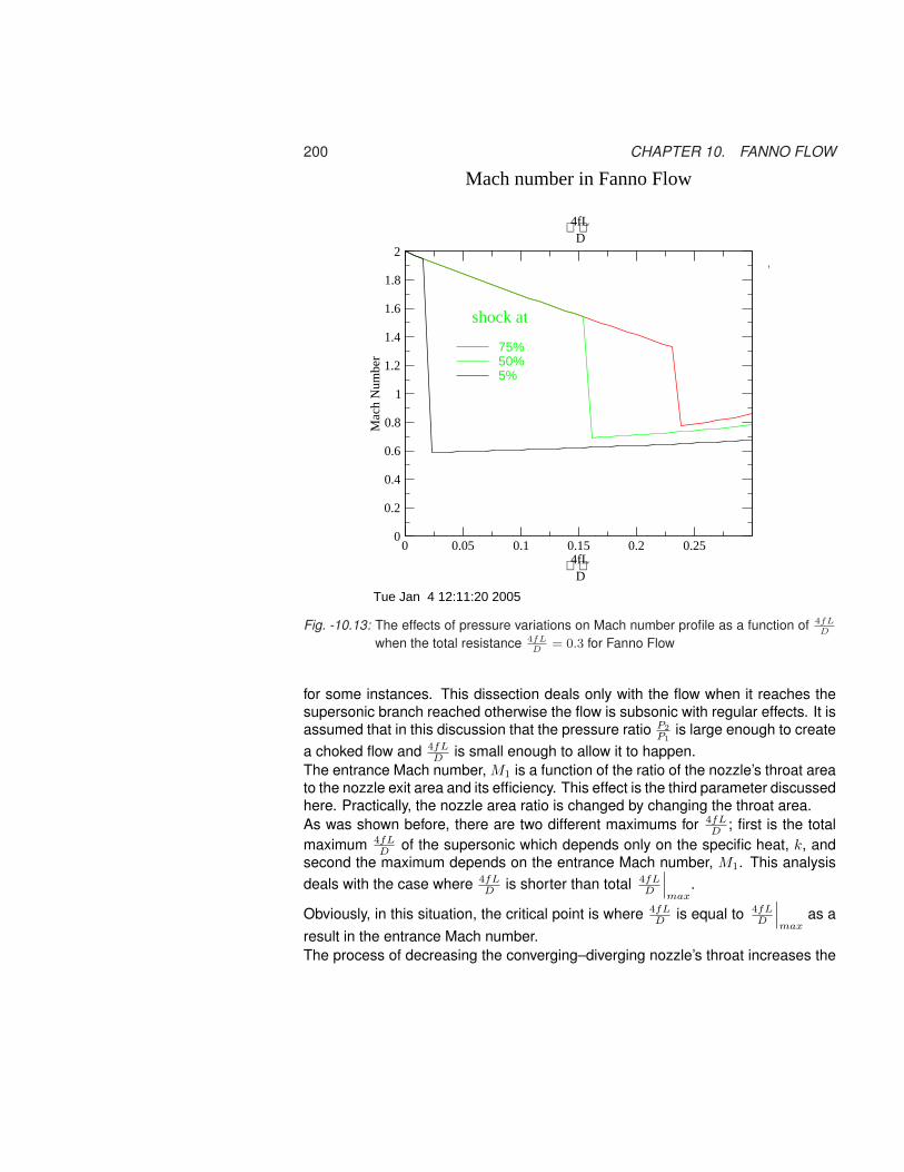
200 CHAPTER 10. FANNO FLOW
0 0.05 0.1 0.15 0.2 0.25
4fLD
0
0.2
0.4
0.6
0.8
1
1.2
1.4
1.6
1.8
2
Mac
h N
umbe
r
75% 50%5%
Mach number in Fanno Flow
4fLD
shock at
Tue Jan 4 12:11:20 2005
Fig. -10.13: The effects of pressure variations on Mach number profile as a function of 4fLD
when the total resistance 4fLD
= 0.3 for Fanno Flow
for some instances. This dissection deals only with the flow when it reaches thesupersonic branch reached otherwise the flow is subsonic with regular effects. It isassumed that in this discussion that the pressure ratio P2
P1is large enough to create
a choked flow and 4fLD is small enough to allow it to happen.
The entrance Mach number, M1 is a function of the ratio of the nozzle’s throat areato the nozzle exit area and its efficiency. This effect is the third parameter discussedhere. Practically, the nozzle area ratio is changed by changing the throat area.As was shown before, there are two different maximums for 4fL
D ; first is the totalmaximum 4fL
D of the supersonic which depends only on the specific heat, k, andsecond the maximum depends on the entrance Mach number, M1. This analysisdeals with the case where 4fL
D is shorter than total 4fLD
∣∣∣max
.
Obviously, in this situation, the critical point is where 4fLD is equal to 4fL
D
∣∣∣max
as aresult in the entrance Mach number.The process of decreasing the converging–diverging nozzle’s throat increases the

10.9. WORKING CONDITIONS 201
0 0.05 0.1 0.15 0.2 0.25
4fLD
0
0.4
0.8
1.2
1.6
2
2.4
2.8
3.2
3.6
4
4.4
4.8
P2/P
1
5 %50 %75 %
P2/P1 Fanno Flow
4fLD
Fri Nov 12 04:07:34 2004
Fig. -10.14: Mach number as a function of 4fLD
when the total 4fLD
= 0.3
entrance14 Mach number. If the tube contains no supersonic flow then reducingthe nozzle throat area wouldn’t increase the entrance Mach number.This part is for the case where some part of the tube is under supersonic regimeand there is shock as a transition to subsonic branch. Decreasing the nozzle throatarea moves the shock location downstream. The “payment” for increase in thesupersonic length is by reducing the mass flow. Further, decrease of the throatarea results in flushing the shock out of the tube. By doing so, the throat area de-creases. The mass flow rate is proportionally linear to the throat area and thereforethe mass flow rate reduces. The process of decreasing the throat area also resultsin increasing the pressure drop of the nozzle (larger resistance in the nozzle15)16.
14The word “entrance” referred to the tube and not to the nozzle. The reference to the tube is becauseit is the focus of the study.
15Strange? Frictionless nozzle has a larger resistance when the throat area decreases16It is one of the strange phenomenon that in one way increasing the resistance (changing the throat
area) decreases the flow rate while in a different way (increasing the 4fLD
) does not affect the flow rate.

202 CHAPTER 10. FANNO FLOW
M = 1M =1 or lessshock
Mx My
4fLD �������max1 � 0B�4fLD 1CA4fLD �������retreat
Fig. -10.15: Schematic of a “long” tube in supersonic branch
In the case of large tube 4fLD > 4fL
D
∣∣∣max
the exit Mach number increases with thedecrease of the throat area. Once the exit Mach number reaches one no furtherincreases is possible. However, the location of the shock wave approaches to thetheoretical location if entrance Mach, M1 = ∞.
4fLD �������retreat
� 0B�4fLD 1CA
4fLD �������max0
M1 =1M1 = 8M1 = 5
Fig. -10.16: The extra tube length as a function of the shock location, 4fLD
supersonic branch
The maximum location of the shock The main point in this discussion how-ever, is to find the furthest shock location downstream. Figure (10.16) shows thepossible ∆
(4fLD
)as function of retreat of the location of the shock wave from the

10.9. WORKING CONDITIONS 203
maximum location. When the entrance Mach number is infinity, M1 = ∞, if theshock location is at the maximum length, then shock at Mx = 1 results in My = 1.The proposed procedure is based on Figure (10.16).
i) Calculate the extra 4fLD and subtract the actual extra 4fL
D assuming shock atthe left side (at the max length).
ii) Calculate the extra 4fLD and subtract the actual extra 4fL
D assuming shock atthe right side (at the entrance).
iii) According to the positive or negative utilizes your root finding procedure.
4fLD4fL
D
∣
∣
∣
∣
∣
∣
∣
max∞
M1max
1
Fig. -10.17: The maximum entrance Mach number, M1 to the tube as a function of 4fLD
supersonic branch
From numerical point of view, the Mach number equal infinity when left side as-sumes result in infinity length of possible extra (the whole flow in the tube is sub-sonic). To overcome this numerical problem it is suggested to start the calculationfrom ε distance from the right hand side.Let denote
∆(
4fL
D
)=
¯4fL
D actual− 4fL
D
∣∣∣∣sup
(10.51)
Note that 4fLD
∣∣∣sup
is smaller than 4fLD
∣∣∣max∞
. The requirement that has to be
satisfied is that denote 4fLD
∣∣∣retreat
as difference between the maximum possible

204 CHAPTER 10. FANNO FLOW
of length in which the supersonic flow is achieved and the actual length in whichthe flow is supersonic see Figure (10.15). The retreating length is expressed assubsonic but
4fL
D
∣∣∣∣retreat
=4fL
D
∣∣∣∣max∞
− 4fL
D
∣∣∣∣sup
(10.52)
Figure (10.17) shows the entrance Mach number, M1 reduces after the maximumlength is exceeded.
Example 10.3:Calculate the shock location for entrance Mach number M1 = 8 and for 4fL
D = 0.9assume that k = 1.4 (Mexit = 1).
SOLUTION
The solution is obtained by an iterative process. The maximum 4fLD
∣∣∣max
for k = 1.4
is 0.821508116. Hence, 4fLD exceed the maximum length 4fL
D for this entranceMach number. The maximum for M1 = 8 is 4fL
D = 0.76820, thus the extra tube
is ∆(
4fLD
)= 0.9 − 0.76820 = 0.1318. The left side is when the shock occurs at
4fLD = 0.76820 (flow is choked and no additional 4fL
D ). Hence, the value of left sideis −0.1318. The right side is when the shock is at the entrance at which the extra4fLD is calculated for Mx and My is
Mx MyTy
Tx
ρy
ρx
Py
Px
P0y
P0x
8.0000 0.39289 13.3867 5.5652 74.5000 0.00849
With (M1)′
M 4fLD
PP∗
P0
P0∗
ρρ∗
UU∗
TT∗
0.39289 2.4417 2.7461 1.6136 2.3591 0.42390 1.1641
The extra ∆(
4fLD
)is 2.442 − 0.1318 = 2.3102 Now the solution is somewhere
between the negative of left side to the positive of the right side17.In a summary of the actions is done by the following algorithm:
(a) check if the 4fLD exceeds the maximum 4fL
D maxfor the supersonic flow.
Accordingly continue.
(b) Guess 4fLD up
= 4fLD − 4fL
D
∣∣∣max
17What if the right side is also negative? The flow is chocked and shock must occur in the nozzlebefore entering the tube. Or in a very long tube the whole flow will be subsonic.

10.9. WORKING CONDITIONS 205
(c) Calculate the Mach number corresponding to the current guess of 4fLD up
,
(d) Calculate the associate Mach number, Mx with the Mach number, My cal-culated previously,
(e) Calculate 4fLD for supersonic branch for the Mx
(f) Calculate the “new and improved” 4fLD up
(g) Compute the “new 4fLD down
= 4fLD − 4fL
D up
(h) Check the new and improved 4fLD
∣∣∣down
against the old one. If it is satisfac-tory stop or return to stage (b).
Shock location are:
M1 M24fLD
∣∣up
4fLD
∣∣down
Mx My
8.0000 1.0000 0.57068 0.32932 1.6706 0.64830
The iteration summary is also shown below
i 4fLD
∣∣up
4fLD
∣∣down
Mx My4fLD
0 0.67426 0.22574 1.3838 0.74664 0.900001 0.62170 0.27830 1.5286 0.69119 0.900002 0.59506 0.30494 1.6021 0.66779 0.900003 0.58217 0.31783 1.6382 0.65728 0.900004 0.57605 0.32395 1.6554 0.65246 0.900005 0.57318 0.32682 1.6635 0.65023 0.900006 0.57184 0.32816 1.6673 0.64920 0.900007 0.57122 0.32878 1.6691 0.64872 0.900008 0.57093 0.32907 1.6699 0.64850 0.900009 0.57079 0.32921 1.6703 0.64839 0.90000
10 0.57073 0.32927 1.6705 0.64834 0.9000011 0.57070 0.32930 1.6706 0.64832 0.9000012 0.57069 0.32931 1.6706 0.64831 0.9000013 0.57068 0.32932 1.6706 0.64831 0.9000014 0.57068 0.32932 1.6706 0.64830 0.9000015 0.57068 0.32932 1.6706 0.64830 0.9000016 0.57068 0.32932 1.6706 0.64830 0.9000017 0.57068 0.32932 1.6706 0.64830 0.90000
This procedure rapidly converted to the solution.

206 CHAPTER 10. FANNO FLOW
10.10 The Practical Questions and Examples of Sub-sonic branch
The Fanno is applicable also when the flow isn’t choke18. In this case, severalquestions appear for the subsonic branch. This is the area shown in Figure (10.8)in beginning for between points 0 and a. This kind of questions made of pairgiven information to find the conditions of the flow, as oppose to only one piece ofinformation given in choked flow. There many combinations that can appear in thissituation but there are several more physical and practical that will be discussedhere.
10.10.1 Subsonic Fanno Flow for Given 4fLD
and Pressure Ratio
P2
M2
∆4fL
D
4fL
D
M1
P1
M = 1
P = P ∗
hypothetical section
Fig. -10.18: Unchoked flow calculations showingthe hypothetical “full” tub when choked
This pair of parameters is themost natural to examine because,in most cases, this information isthe only information that is pro-vided. For a given pipe
(4fLD
),
neither the entrance Mach num-ber nor the exit Mach number aregiven (sometimes the entranceMach number is give see the next section). There is no exact analytical solution.There are two possible approaches to solve this problem: one, by building a rep-resentative function and find a root (or roots) of this representative function. Two,the problem can be solved by an iterative procedure. The first approach requireusing root finding method and either method of spline method or the half methodfound to be good. However, this author experience show that these methods inthis case were found to be relatively slow. The Newton–Rapson method is muchfaster but not were found to be unstable (at lease in the way that was implementedby this author). The iterative method used to solve constructed on the propertiesof several physical quantities must be in a certain range.. The first fact is that thepressure ratio P2/P1 is always between 0 and 1 (see Figure (10.18)). In the figure,a theoretical extra tube is added in such a length that cause the flow to choke (if itreally was there). This length is always positive (at minimum is zero).
The procedure for the calculations is as the following:
1) Calculate the entrance Mach number, M1
′assuming the 4fL
D = 4fLD
∣∣∣max
′
(chocked flow);
2) Calculate the minimum pressure ratio (P2/P1)min for M1
′(look at table (10.1))
18This questions were raised from many who didn’t found any book that discuss these practical as-pects and send questions to this author.

10.10. PRACTICAL EXAMPLES FOR SUBSONIC FLOW 207
3) Check if the flow is choked:There are two possibilities to check it.
a) Check if the given 4fLD is smaller than 4fL
D obtained from the given P1/P2, or
b) check if the (P2/P1)min is larger than (P2/P1),
continue if the criteria is satisfied. Or if not satisfied abort this procedureand continue to calculation for choked flow.
4) Calculate the M2 based on the (P ∗/P2) = (P1/P2),
5) calculate ∆ 4fLD based on M2,
6) calculate the new (P2/P1), based on the new f((
4fLD
)1,(
4fLD
)2
),
(remember that ∆4fLD =
(4fLD
)2),
7) calculate the corresponding M1 and M2,
8) calculate the new and “improve” the ∆4fLD by
(∆
4fL
D
)
new
=(
∆4fL
D
)
old
∗
(P2P1
)given(
P2P1
)old
(10.53)
Note, when the pressure ratios are matching also the ∆4fLD will also match.
9) Calculate the “improved/new” M2 based on the improve ∆ 4fLD
10) calculate the improved 4fLD as 4fL
D =(
4fLD
)given
+ ∆(
4fLD
)new
11) calculate the improved M1 based on the improved 4fLD .
12) Compare the abs ((P2/P1)new − (P2/P1)old ) and if not satisfiedreturned to stage (6) until the solution is obtained.
To demonstrate how this procedure is working consider a typical example of 4fLD =
1.7 and P2/P1 = 0.5. Using the above algorithm the results are exhibited in thefollowing figure. Figure (10.19) demonstrates that the conversion occur at about7-8 iterations. With better first guess this conversion procedure will converts muchfaster (under construction).

208 CHAPTER 10. FANNO FLOW
0 10 20 30 40 50 60 70 80 90 100 110 120 130
Number of Iterations,
0.5
1.0
1.5
2.0
2.5
3.0
M1
M2
P2/P1
Conversion occurs around 7-9 times
i
4fL
D
∆4fL
D
October 8, 2007
Fig. -10.19: The results of the algorithm showing the conversion rate for unchoked Fannoflow model with a given 4fL
Dand pressure ratio.
10.10.2 Subsonic Fanno Flow for a Given M1 and Pressure Ra-tio
This situation pose a simple mathematical problem while the physical situationoccurs in cases where a specific flow rate is required with a given pressure ratio(range) (this problem was considered by some to be somewhat complicated). Thespecific flow rate can be converted to entrance Mach number and this simplifiesthe problem. Thus, the problem is reduced to find for given entrance Mach, M1,and given pressure ratio calculate the flow parameters, like the exit Mach number,M2. The procedure is based on the fact that the entrance star pressure ratio canbe calculated using M1. Thus, using the pressure ratio to calculate the star exitpressure ratio provide the exit Mach number, M2. An example of such issue is thefollowing example that combines also the “Naughty professor” problems.
Example 10.4:Calculate the exit Mach number for P2/P1 = 0.4 and entrance Mach number M1 =0.25.
SOLUTIONThe star pressure can be obtained from a table or Potto-GDC as
M 4fLD
PP∗
P0
P0∗
ρρ∗
UU∗
TT∗
0.25000 8.4834 4.3546 2.4027 3.6742 0.27217 1.1852
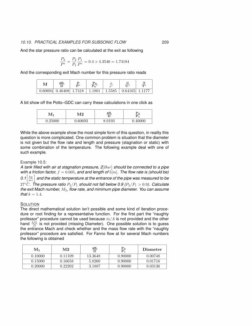
10.10. PRACTICAL EXAMPLES FOR SUBSONIC FLOW 209
And the star pressure ratio can be calculated at the exit as following
P2
P ∗=
P2
P1
P1
P ∗= 0.4× 4.3546 = 1.74184
And the corresponding exit Mach number for this pressure ratio reads
M 4fLD
PP∗
P0
P0∗
ρρ∗
UU∗
TT∗
0.60694 0.46408 1.7418 1.1801 1.5585 0.64165 1.1177
A bit show off the Potto–GDC can carry these calculations in one click as
M1 M2 4fLD
P2
P1
0.25000 0.60693 8.0193 0.40000
While the above example show the most simple form of this question, in reality thisquestion is more complicated. One common problem is situation that the diameteris not given but the flow rate and length and pressure (stagnation or static) withsome combination of the temperature. The following example deal with one ofsuch example.
Example 10.5:A tank filled with air at stagnation pressure, 2[Bar] should be connected to a pipewith a friction factor, f = 0.005, and and length of 5[m]. The flow rate is (should be)0.1
[kgsec
]and the static temperature at the entrance of the pipe was measured to be
27◦C. The pressure ratio P2/P1 should not fall below 0.9 (P2/P1 > 0.9). Calculatethe exit Mach number, M2, flow rate, and minimum pipe diameter. You can assumethat k = 1.4.
SOLUTIONThe direct mathematical solution isn’t possible and some kind of iteration proce-dure or root finding for a representative function. For the first part the “naughtyprofessor” procedure cannot be used because m/A is not provided and the otherhand 4fL
D is not provided (missing Diameter). One possible solution is to guessthe entrance Mach and check whether and the mass flow rate with the “naughtyprofessor” procedure are satisfied. For Fanno flow at for several Mach numbersthe following is obtained
M1 M2 4fLD
P2
P1Diameter
0.10000 0.11109 13.3648 0.90000 0.007480.15000 0.16658 5.8260 0.90000 0.017160.20000 0.22202 3.1887 0.90000 0.03136

210 CHAPTER 10. FANNO FLOW
0.1 0.15 0.2 0.25 0.3
Conversion of the guesing the Mach Number
0.1
0.2
0.3
0.4
Ent
race
Mac
hN
ubm
er
guessedcalculated
Solution
M1
M1
October 18, 2007
Fig. -10.20: Diagram for finding solution when the pressure ratio and entrance properties (Tand P0 are given
From the last table the diameter can be calculated for example for M1 = 0.2 as
D =4fL4fLD
= 4× 0.005× 5/3.1887 = 0.03136[m]
The same was done for all the other Mach number. Now the area can be calcu-lated and therefor the m/A can be calculated. With this information the “naughtyprofessor” is given and the entrance Mach number can be calculated. For examplefor M1 = 0.2 one can obtain the following:
m/A = 0.1/(π × 0.031362/4) ∼ 129.4666798
The same order as the above table it shown in “naughty professor” (isentropictable).
M TT0
ρρ0
AA?
PP0
A×PA∗×P0
FF∗
1.5781 0.66752 0.36404 1.2329 0.24300 0.29960 0.560090.36221 0.97443 0.93730 1.7268 0.91334 1.5772 0.777850.10979 0.99760 0.99400 5.3092 0.99161 5.2647 2.2306
The first result are not reasonable and this process can continue until the satisfac-tory solution is achieved. Here an graphical approximation is shown.From this exhibit it can be estimated that M1 = 0.18. For this Mach number thefollowing can be obtained
M1 M2 4fLD
P2
P1
0.18000 0.19985 3.9839 0.90000
Thus, the diameter can be obtained as D ∼ 0.0251[m]The flow rate is m/A ∼ 202.1[kg/sec×m2]

10.11. THE APPROXIMATION OF THE FANNO FLOW BY ISOTHERMAL FLOW211
M TT0
ρρ0
AA?
PP0
A×PA∗×P0
FF∗
0.17109 0.99418 0.98551 3.4422 0.97978 3.3726 1.4628
The exact solution is between 0.17 to 0.18 if better accuracy is needed.
10.11 The Approximation of the Fanno Flow by Isother-mal Flow
The isothermal flow model has equations that theoreticians find easier to use andto compare to the Fanno flow model.One must notice that the maximum temperature at the entrance is T01. When theMach number decreases the temperature approaches the stagnation temperature(T → T0). Hence, if one allows certain deviation of temperature, say about 1% thatflow can be assumed to be isothermal. This tolerance requires that (T0 − T )/T0 =0.99 which requires that enough for M1 < 0.15 even for large k = 1.67. Thisrequirement provides that somewhere (depend) in the vicinity of 4fL
D = 25 the flowcan be assumed isothermal. Hence the mass flow rate is a function of 4fL
D becauseM1 changes. Looking at the table or Figure (10.2) or the results from Potto–GDCattached to this book shows that reduction of the mass flow is very rapid. As itcan be seen for the Figure (10.21) the dominating parameter is 4fL
D . The resultsare very similar for isothermal flow. The only difference is in small dimensionlessfriction, 4fL
D .
10.12 More Examples of Fanno FlowExample 10.6:To demonstrate the utility in Figure (10.21) consider the following example. Findthe mass flow rate for f = 0.05, L = 4[m], D = 0.02[m] and pressure ratio P2/P1 =0.1, 0.3, 0.5, 0.8. The stagnation conditions at the entrance are 300K and 3[bar] air.
SOLUTIONFirst calculate the dimensionless resistance, 4fL
D .
4fL
D=
4× 0.05× 40.02
= 40
From Figure (10.21) for P2/P1 = 0.1 M1 ≈ 0.13 etc.or accurately by utilizing the program as in the following table.
M1 M24fLD
4fLD
∣∣1
4fLD
∣∣2
P2
P1
0.12728 1.0000 40.0000 40.0000 0.0 0.116370.12420 0.40790 40.0000 42.1697 2.1697 0.300000.11392 0.22697 40.0000 50.7569 10.7569 0.500000.07975 0.09965 40.0000 107.42 67.4206 0.80000

212 CHAPTER 10. FANNO FLOW
0 10 20 30 40 50 60 70 80 90 100
4fLD
0
0.1
0.2
0.3
0.4
M1
P2 / P
1 = 0.1 iso
P2 / P
1 = 0.8 iso
P2 / P
1 = 0.1
P2 / P
1 = 0.2
P2 / P
1 = 0.5
P2 / P
1 = 0.8
M1 Fanno flow
with comperison to Isothermal Flow
Wed Mar 9 11:38:27 2005
Fig. -10.21: The entrance Mach number as a function of dimensionless resistance and com-parison with Isothermal Flow
Only for the pressure ratio of 0.1 the flow is choked.
M TT0
ρρ0
AA?
PP0
A×PA∗×P0
0.12728 0.99677 0.99195 4.5910 0.98874 4.53930.12420 0.99692 0.99233 4.7027 0.98928 4.65230.11392 0.99741 0.99354 5.1196 0.99097 5.07330.07975 0.99873 0.99683 7.2842 0.99556 7.2519
Therefore, T ≈ T0 and is the same for the pressure. Hence, the mass rate isa function of the Mach number. The Mach number is indeed a function of thepressure ratio but mass flow rate is a function of pressure ratio only through Machnumber.The mass flow rate is
m = PAM
√k
RT= 300000× π × 0.022
4× 0.127×
√1.4
287300≈ 0.48
(kg
sec
)

10.13. THE TABLE FOR FANNO FLOW 213
and for the rest
m
(P2
P1= 0.3
)∼ 0.48× 0.1242
0.1273= 0.468
(kg
sec
)
m
(P2
P1= 0.5
)∼ 0.48× 0.1139
0.1273= 0.43
(kg
sec
)
m
(P2
P1= 0.8
)∼ 0.48× 0.07975
0.1273= 0.30
(kg
sec
)
10.13 The Table for Fanno Flow
Table -10.1: Fanno Flow Standard basic Table
M 4fLD
PP∗
P0
P0∗
ρρ∗
UU∗
TT∗
0.03 787.08 36.5116 19.3005 30.4318 0.03286 1.19980.04 440.35 27.3817 14.4815 22.8254 0.04381 1.19960.05 280.02 21.9034 11.5914 18.2620 0.05476 1.19940.06 193.03 18.2508 9.6659 15.2200 0.06570 1.19910.07 140.66 15.6416 8.2915 13.0474 0.07664 1.19880.08 106.72 13.6843 7.2616 11.4182 0.08758 1.19850.09 83.4961 12.1618 6.4613 10.1512 0.09851 1.19810.10 66.9216 10.9435 5.8218 9.1378 0.10944 1.19760.20 14.5333 5.4554 2.9635 4.5826 0.21822 1.19050.25 8.4834 4.3546 2.4027 3.6742 0.27217 1.18520.30 5.2993 3.6191 2.0351 3.0702 0.32572 1.17880.35 3.4525 3.0922 1.7780 2.6400 0.37879 1.17130.40 2.3085 2.6958 1.5901 2.3184 0.43133 1.16280.45 1.5664 2.3865 1.4487 2.0693 0.48326 1.15330.50 1.0691 2.1381 1.3398 1.8708 0.53452 1.14290.55 0.72805 1.9341 1.2549 1.7092 0.58506 1.13150.60 0.49082 1.7634 1.1882 1.5753 0.63481 1.11940.65 0.32459 1.6183 1.1356 1.4626 0.68374 1.10650.70 0.20814 1.4935 1.0944 1.3665 0.73179 1.09290.75 0.12728 1.3848 1.0624 1.2838 0.77894 1.07870.80 0.07229 1.2893 1.0382 1.2119 0.82514 1.06380.85 0.03633 1.2047 1.0207 1.1489 0.87037 1.04850.90 0.01451 1.1291 1.0089 1.0934 0.91460 1.03270.95 0.00328 1.061 1.002 1.044 0.95781 1.0171.00 0.0 1.00000 1.000 1.000 1.00 1.0002.00 0.30500 0.40825 1.688 0.61237 1.633 0.666673.00 0.52216 0.21822 4.235 0.50918 1.964 0.42857

214 CHAPTER 10. FANNO FLOW
Table -10.1: Fanno Flow Standard basic Table (continue)
M 4fLD
PP∗
P0
P0∗
ρρ∗
UU∗
TT∗
4.00 0.63306 0.13363 10.72 0.46771 2.138 0.285715.00 0.69380 0.089443 25.00 0.44721 2.236 0.200006.00 0.72988 0.063758 53.18 0.43568 2.295 0.146347.00 0.75280 0.047619 1.0E+2 0.42857 2.333 0.111118.00 0.76819 0.036860 1.9E+2 0.42390 2.359 0.0869579.00 0.77899 0.029348 3.3E+2 0.42066 2.377 0.069767
10.00 0.78683 0.023905 5.4E+2 0.41833 2.390 0.05714320.00 0.81265 0.00609 1.5E+4 0.41079 2.434 0.01481525.00 0.81582 0.00390 4.6E+4 0.40988 2.440 0.0095230.00 0.81755 0.00271 1.1E+5 0.40938 2.443 0.0066335.00 0.81860 0.00200 2.5E+5 0.40908 2.445 0.0048840.00 0.81928 0.00153 4.8E+5 0.40889 2.446 0.0037445.00 0.81975 0.00121 8.6E+5 0.40875 2.446 0.0029650.00 0.82008 0.000979 1.5E+6 0.40866 2.447 0.0024055.00 0.82033 0.000809 2.3E+6 0.40859 2.447 0.0019860.00 0.82052 0.000680 3.6E+6 0.40853 2.448 0.0016665.00 0.82066 0.000579 5.4E+6 0.40849 2.448 0.0014270.00 0.82078 0.000500 7.8E+6 0.40846 2.448 0.00122
10.14 AppendixThe friction factor in equation (10.25) was assumed constant. In Chapter 9 it wasshown that the Reynolds number remains constant for ideal gas fluid. However, inFanno flow the temperature does not remain constant hence as it was discussedbefore the Reynolds number is increasing. Thus, the friction decreases with theexception of the switch in the flow pattern (laminar to turbulent flow). For relativelylarge relative roughness larger ε/D > 0.004 of 0.4% the friction factor is constant.For smother pipe ε/D < 0.001 and Reynolds number between 10,000 to a millionthe friction factor vary between 0.007 to 0.003 with is about factor of two. Thus,the error of 4fL
D is limited by a factor of two (2). For this range, the friction factorcan be estimated as a linear function of the log10(Re). The error in this assumptionis probably small of the assumption that involve in fanno flow model construction.Hence,
f = A log10(Re) + B (10.54)
Where the constant A and B are function of the relative roughness. For mostpractical purposes the slop coefficient A can be further assumed constant. Theslop coefficient A = −0.998125 Thus, to carry this calculation relationship betweenthe viscosity and the temperature. If the viscosity expanded as Taylor or Maclaren

10.14. APPENDIX 215
Almost Constant Zone
Constant Zone
Linear RepresentationZone
Small ErrorDue to Linear Assumption
Fig. -10.22: “Moody” diagram on the name Moody who netscape H. Rouse work to claimas his own. In this section the turbulent area is divided into 3 zones, constant,semi–constant, and linear After S Beck and R. Collins.
series then
µ
µ1= A0 +
A1 T
T0+ · · · (10.55)
Where µ1 is the viscosity at the entrance temperature T1.Thus, Reynolds number is
Re =D ρU
A0 + A1 TT0
+ · · · (10.56)
Substituting equation (10.56) into equation (10.54) yield
f = A log10
(D ρU
A0 + A1 T2T1
+ · · ·
)+ B (10.57)
Left hand side of equation (10.25) is a function of the Mach number since it con-tains the temperature. If the temperature functionality will not vary similarly to thecase of constant friction factor then the temperature can be expressed using equa-tion (10.41).
4D
A log10
constant︷ ︸︸ ︷D ρ U
A0 + A1
1 + k−12 M1
2
1 + k−12 M2
2 + · · ·
+ B
(10.58)

216 CHAPTER 10. FANNO FLOW
Equation (10.58) is only estimate of the functionally however, this estimate is al-most as good as the assumptions of Fanno flow. Equation fanno:eq:fld2 can beimproved by using equation (10.58)
4 Lmax
D
A log10
constant︷ ︸︸ ︷D ρ U
A0 + A1
1 + k−12 M2
1 + k−12
+ B
∼ 1
k
1−M2
M2+
k + 12k
lnk+12 M2
1 + k−12 M2
(10.59)
In the most complicate case where the flow pattern is change from laminar flowto turbulent flow the whole Fanno flow model is questionable and will produce poorresults.In summary, in the literature there are three approaches to this issue of non con-stant friction factor. The friction potential is recommended by a researcher in Ger-many and it is complicated. The second method substituting this physical approachwith numerical iteration. In the numerical iteration method, the expression of thevarious relationships are inserted into governing differential equations. The nu-merical methods does not allow flexibility and is very complicated. The methodsdescribed here can be expended (if really really needed) and it will be done in veryfew iteration as it was shown in the Isothermal Chapter.

CHAPTER 11
Rayleigh Flow
Rayleigh flow is model describing a frictionless flow with heat transfer through apipe of constant cross sectional area. In practice Rayleigh flow isn’t a really goodmodel for the real situation. Yet, Rayleigh flow is practical and useful conceptin a obtaining trends and limits such as the density and pressure change due toexternal cooling or heating. As opposed to the two previous models, the heattransfer can be in two directions not like the friction (there is no negative friction).This fact creates a situation different as compare to the previous two models. Thismodel can be applied to cases where the heat transfer is significant and the frictioncan be ignored.
11.1 Introduction
�1P1 �2P2T1 T2heat transfer (in and out)
flowdirection
QFig. -11.1: The control volume of
Rayleigh Flow
The third simple model for one–dimensional flow with constant heat transferfor frictionless flow. This flow is referred inthe literature as Rayleigh Flow (see historicalnotes). This flow is another extreme case inwhich the friction effect is neglected becausetheir relative effect is much smaller than theheat transfer effect. While the isothermal flowmodel has heat transfer and friction, the mainassumption was that relative length is enables significant heat transfer to occurbetween the surroundings and tube. In contrast, the heat transfer in Rayleigh flowoccurs between unknown temperature and the tube and the heat flux is maintainedconstant. As before, a simple model is built around the assumption of constantproperties (poorer prediction to case where chemical reaction take a place).
217
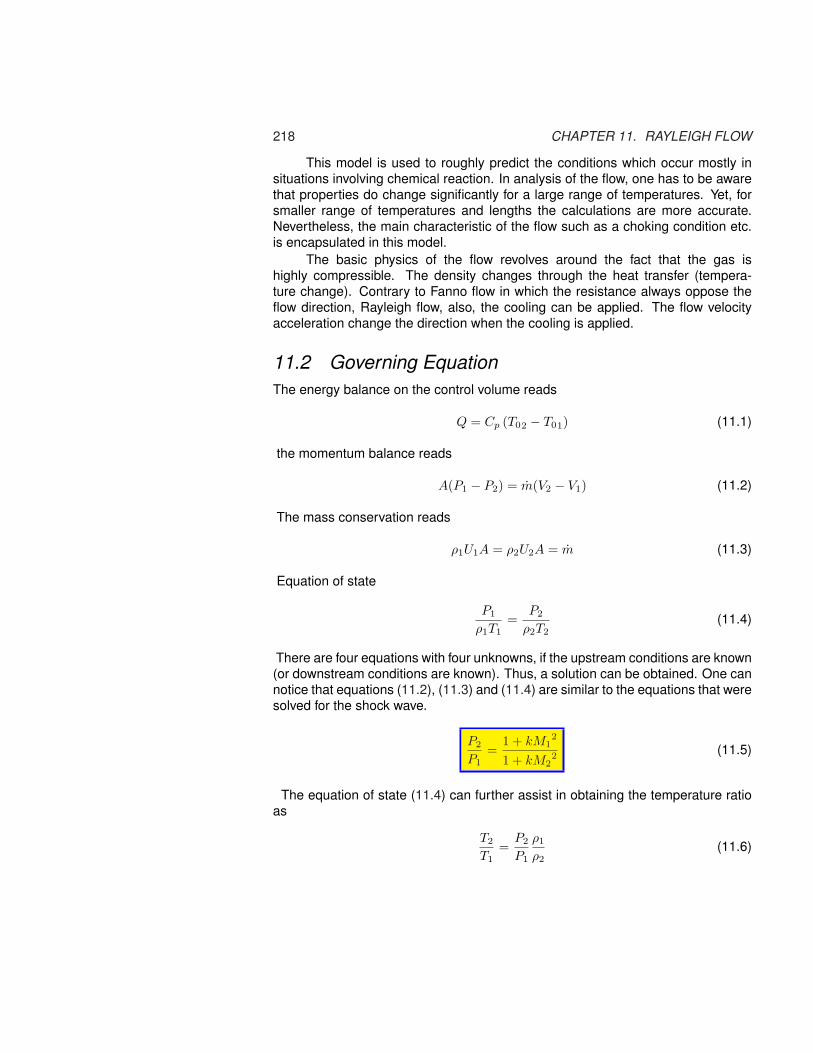
218 CHAPTER 11. RAYLEIGH FLOW
This model is used to roughly predict the conditions which occur mostly insituations involving chemical reaction. In analysis of the flow, one has to be awarethat properties do change significantly for a large range of temperatures. Yet, forsmaller range of temperatures and lengths the calculations are more accurate.Nevertheless, the main characteristic of the flow such as a choking condition etc.is encapsulated in this model.
The basic physics of the flow revolves around the fact that the gas ishighly compressible. The density changes through the heat transfer (tempera-ture change). Contrary to Fanno flow in which the resistance always oppose theflow direction, Rayleigh flow, also, the cooling can be applied. The flow velocityacceleration change the direction when the cooling is applied.
11.2 Governing EquationThe energy balance on the control volume reads
Q = Cp (T02 − T01) (11.1)
the momentum balance reads
A(P1 − P2) = m(V2 − V1) (11.2)
The mass conservation reads
ρ1U1A = ρ2U2A = m (11.3)
Equation of state
P1
ρ1T1=
P2
ρ2T2(11.4)
There are four equations with four unknowns, if the upstream conditions are known(or downstream conditions are known). Thus, a solution can be obtained. One cannotice that equations (11.2), (11.3) and (11.4) are similar to the equations that weresolved for the shock wave.
P2
P1=
1 + kM12
1 + kM22 (11.5)
The equation of state (11.4) can further assist in obtaining the temperature ratioas
T2
T1=
P2
P1
ρ1
ρ2(11.6)

11.2. GOVERNING EQUATION 219
The density ratio can be expressed in terms of mass conservation as
ρ1
ρ2=
U2
U1=
U2rkRT2
√kRT2
U1rkRT1
√kRT1
=M2
M1
√T2
T1(11.7)
or
ρ1
ρ2=
U2
U1=
M2
M1
√T2
T1 (11.8)
or Substituting equations (11.5) and (11.8) into equation (11.6) yields
T2
T1=
1 + kM12
1 + kM22
M2
M1
√T2
T1(11.9)
Transferring the temperature ratio to the left hand side and squaring the resultsgives
T2
T1=
[1 + kM1
2
1 + kM22
]2 (M2
M1
)2
(11.10)
T
s
M = 1pkM = 1
M > 1
M < 1
constant Pressure line
P = P �
Fig. -11.2: The temperature entropy diagram for Rayleigh line
The Rayleigh line exhibits two possible maximums one for dT/ds = 0 and fords/dT = 0. The second maximum can be expressed as dT/ds = ∞. The second

220 CHAPTER 11. RAYLEIGH FLOW
law is used to find the expression for the derivative.
s1 − s2
Cp= ln
T2
T1− k − 1
kln
P2
P1(11.11)
s1 − s2
Cp= 2 ln
[(
1 + kM12)
(1 + kM22)
M2
M1
]+
k − 1k
ln[1 + kM212
1 + kM12
]
(11.12)
Let the initial condition M1, and s1 be constant and the variable parameters areM2, and s2. A derivative of equation (11.12) results in
1Cp
ds
dM=
2(1−M2)M(1 + kM2)
(11.13)
Taking the derivative of equation (11.13) and letting the variable parameters beT2, and M2 results in
dT
dM= constant× 1− kM2
(1 + kM2)3(11.14)
Combining equations (11.13) and (11.14) by eliminating dM results in
dT
ds= constant× M(1− kM2)
(1−M2)(1 + kM2)2(11.15)
On T-s diagram a family of curves can be drawn for a given constant. Yet for everycurve, several observations can be generalized. The derivative is equal to zerowhen 1−kM2 = 0 or M = 1/
√k or when M → 0. The derivative is equal to infinity,
dT/ds = ∞ when M = 1. From thermodynamics, increase of heating results inincrease of entropy. And cooling results in reduction of entropy. Hence, whencooling is applied to a tube the velocity decreases and when heating is applied thevelocity increases. At peculiar point of M = 1/
√k when additional heat is applied
the temperature decreases. The derivative is negative, dT/ds < 0, yet note thispoint is not the choking point. The choking occurs only when M = 1 because itviolates the second law. The transition to supersonic flow occurs when the areachanges, somewhat similarly to Fanno flow. Yet, choking can be explained by thefact that increase of energy must be accompanied by increase of entropy. Butthe entropy of supersonic flow is lower (see Figure (11.2)) and therefore it is notpossible (the maximum entropy at M = 1.).
It is convenient to refer to the value of M = 1. These values are referred toas the “star”1 values. The equation (11.5) can be written between choking pointand any point on the curve.
P ∗
P1=
1 + kM12
1 + k (11.16)1The star is an asterisk.

11.3. RAYLEIGH FLOW TABLES 221
The temperature ratio is
T ∗
T1=
1M2
(1 + kM1
2
1 + k
)2
(11.17)
ρ1
ρ∗=
U∗
U1=
U∗√kRT∗
√kRT ∗
U1√kRT1
√kRT1
(11.18)
or
ρ1
ρ∗=
U∗
U1=
1M1
√T ∗
T1 (11.19)
T01
T0∗ =
T1
(1 + k−1
2 M12)
T ∗(
1+k2
) (11.20)
or explicitly
T01
T0∗ =
2(1 + k)M12
(1 + kM2)2
(1 +
k − 12
M12
)
(11.21)
The stagnation pressure ratio reads
P01
P0∗ =
P1
(1 + k−1
2 M12)
P ∗(
1+k2
) (11.22)
or explicitly
P01
P0∗ =
(1 + k
1 + kM12
) (1 + kM1
2
(1+k)2
) kk−1
(11.23)
11.3 Rayleigh Flow TablesThe “star” values are tabulated in Table (11.1). Several observations can be madein regards to the stagnation temperature.

222 CHAPTER 11. RAYLEIGH FLOW
Table -11.1: Rayleigh Flow k=1.4
M TT∗
T0
T0∗
PP∗
P0
P0∗
ρ∗
ρ
0.03 0.00517 0.00431 2.397 1.267 0.002160.04 0.00917 0.00765 2.395 1.266 0.003830.05 0.014300 0.011922 2.392 1.266 0.005980.06 0.020529 0.017119 2.388 1.265 0.008600.07 0.027841 0.023223 2.384 1.264 0.0116800.08 0.036212 0.030215 2.379 1.262 0.0152240.09 0.045616 0.038075 2.373 1.261 0.0192220.10 0.056020 0.046777 2.367 1.259 0.0236690.20 0.20661 0.17355 2.273 1.235 0.0909090.25 0.30440 0.25684 2.207 1.218 0.137930.30 0.40887 0.34686 2.131 1.199 0.191830.35 0.51413 0.43894 2.049 1.178 0.250960.40 0.61515 0.52903 1.961 1.157 0.313730.45 0.70804 0.61393 1.870 1.135 0.378650.50 0.79012 0.69136 1.778 1.114 0.444440.55 0.85987 0.75991 1.686 1.094 0.510010.60 0.91670 0.81892 1.596 1.075 0.574470.65 0.96081 0.86833 1.508 1.058 0.637130.70 0.99290 0.90850 1.423 1.043 0.697510.75 1.014 0.94009 1.343 1.030 0.755240.80 1.025 0.96395 1.266 1.019 0.810130.85 1.029 0.98097 1.193 1.011 0.862040.90 1.025 0.99207 1.125 1.005 0.910970.95 1.015 0.99814 1.060 1.001 0.956931.0 1.00 1.00 1.00 1.00 1.0001.1 0.96031 0.99392 0.89087 1.005 1.0781.2 0.91185 0.97872 0.79576 1.019 1.1461.3 0.85917 0.95798 0.71301 1.044 1.2051.4 0.80539 0.93425 0.64103 1.078 1.2561.5 0.75250 0.90928 0.57831 1.122 1.3011.6 0.70174 0.88419 0.52356 1.176 1.3401.7 0.65377 0.85971 0.47562 1.240 1.3751.8 0.60894 0.83628 0.43353 1.316 1.4051.9 0.56734 0.81414 0.39643 1.403 1.4312.0 0.52893 0.79339 0.36364 1.503 1.4552.1 0.49356 0.77406 0.33454 1.616 1.4752.2 0.46106 0.75613 0.30864 1.743 1.4942.3 0.43122 0.73954 0.28551 1.886 1.5102.4 0.40384 0.72421 0.26478 2.045 1.525

11.4. EXAMPLES FOR RAYLEIGH FLOW 223
Table -11.1: Rayleigh Flow k=1.4 (continue)
M TT∗
T0
T0∗
PP∗
P0
P0∗
ρ∗
ρ
2.5 0.37870 0.71006 0.24615 2.222 1.5382.6 0.35561 0.69700 0.22936 2.418 1.5502.7 0.33439 0.68494 0.21417 2.634 1.5612.8 0.31486 0.67380 0.20040 2.873 1.5712.9 0.29687 0.66350 0.18788 3.136 1.5803.0 0.28028 0.65398 0.17647 3.424 1.5883.5 0.21419 0.61580 0.13223 5.328 1.6204.0 0.16831 0.58909 0.10256 8.227 1.6414.5 0.13540 0.56982 0.081772 12.50 1.6565.0 0.11111 0.55556 0.066667 18.63 1.6675.5 0.092719 0.54473 0.055363 27.21 1.6756.0 0.078487 0.53633 0.046693 38.95 1.6816.5 0.067263 0.52970 0.039900 54.68 1.6867.0 0.058264 0.52438 0.034483 75.41 1.6907.5 0.050943 0.52004 0.030094 1.0E+2 1.6938.0 0.044910 0.51647 0.026490 1.4E+2 1.6958.5 0.039883 0.51349 0.023495 1.8E+2 1.6989.0 0.035650 0.51098 0.020979 2.3E+2 1.6999.5 0.032053 0.50885 0.018846 3.0E+2 1.701
10.0 0.028972 0.50702 0.017021 3.8E+2 1.70220.0 0.00732 0.49415 0.00428 1.1E+4 1.71125.0 0.00469 0.49259 0.00274 3.2E+4 1.71230.0 0.00326 0.49174 0.00190 8.0E+4 1.71335.0 0.00240 0.49122 0.00140 1.7E+5 1.71340.0 0.00184 0.49089 0.00107 3.4E+5 1.71445.0 0.00145 0.49066 0.000846 6.0E+5 1.71450.0 0.00117 0.49050 0.000686 1.0E+6 1.71455.0 0.000971 0.49037 0.000567 1.6E+6 1.71460.0 0.000816 0.49028 0.000476 2.5E+6 1.71465.0 0.000695 0.49021 0.000406 3.8E+6 1.71470.0 0.000600 0.49015 0.000350 5.5E+6 1.714
The data is presented in Figure (11.3).
11.4 Examples For Rayleigh FlowIllustrative example
The typical questions that are raised in Rayleigh Flow are related to the max-imum heat that can be transferred to gas (reaction heat) and to the flow rate.

224 CHAPTER 11. RAYLEIGH FLOW
0.1 1 10M
0
1
2
3
4
T / T*
T0
/ T0
*
P / P*
P0 /
P0
*
ρ / ρ∗
Rayleigh Flowk = 1 4
@( M = ) 0.4898∞
@( M = ) 1.7143∞
Fri May 6 11:11:44 2005
Fig. -11.3: The basic functions of Rayleigh Flow (k=1.4)
Example 11.1:Air enters a pipe with pressure of 3[bar] and temperature of 27◦C at Mach numberof M = 0.25. Due to internal combustion heat was released and the exit tempera-ture was found to be 127◦C. Calculate the exit Mach number, the exit pressure, thetotal exit pressure, and heat released and transferred to the air. At what amount ofenergy the exit temperature will start to decrease? Assume CP = 1.004
[kJ
kg◦C
]
SOLUTIONThe entrance Mach number and the exit temperature are given and from Table(11.1) or from the program the initial ratio can be calculated. From the initial valuesthe ratio at the exit can be computed as the following.
M TT∗
T0
T0∗
PP∗
P0
P0∗
ρ∗
ρ
0.25000 0.30440 0.25684 2.2069 1.2177 0.13793

11.4. EXAMPLES FOR RAYLEIGH FLOW 225
andT2
T ∗=
T1
T ∗T2
T1= 0.304× 400
300= 0.4053
M TT∗
T0
T0∗
PP∗
P0
P0∗
ρ∗
ρ
0.29831 0.40530 0.34376 2.1341 1.1992 0.18991
The exit Mach number is known, the exit pressure can be calculated as
P2 = P1P ∗
P1
P2
P ∗= 3× 1
2.2069× 2.1341 = 2.901[Bar]
For the entrance the stagnation values are
M TT0
ρρ0
AA?
PP0
A×PA∗×P0
FF∗
0.25000 0.98765 0.96942 2.4027 0.95745 2.3005 1.0424
The total exit pressure, P02 can be calculated as the following:
P02 = P1
isentropic︷︸︸︷P01
P1
P0∗
P01
P02
P0∗ = 3× 1
0.95745× 1
1.2177× 1.1992 = 3.08572[Bar]
The heat released (heat transferred) can be calculated from obtaining the stag-nation temperature from both sides. The stagnation temperature at the entrance,T01
T01 = T1
isentropic︷︸︸︷T01
T1= 300/0.98765 = 303.75[K]
The isentropic conditions at the exit are
M TT0
ρρ0
AA?
PP0
A×PA∗×P0
FF∗
0.29831 0.98251 0.95686 2.0454 0.94012 1.9229 0.90103
The exit stagnation temperature is
T02 = T2
isentropic︷︸︸︷T02
T2= 400/0.98765 = 407.12[K]
The heat released becomes
Q
m= Cp (T02 − T01) 1× 1.004× (407.12− 303.75) = 103.78
[kJ
seckg◦C
]
The maximum temperature occurs at the point where the Mach number reaches1/√
k and at this point the Rayleigh relationship are:
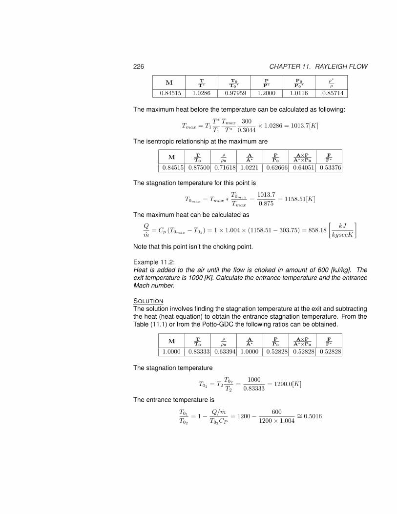
226 CHAPTER 11. RAYLEIGH FLOW
M TT∗
T0
T0∗
PP∗
P0
P0∗
ρ∗
ρ
0.84515 1.0286 0.97959 1.2000 1.0116 0.85714
The maximum heat before the temperature can be calculated as following:
Tmax = T1T ∗
T1
Tmax
T ∗300
0.3044× 1.0286 = 1013.7[K]
The isentropic relationship at the maximum are
M TT0
ρρ0
AA?
PP0
A×PA∗×P0
FF∗
0.84515 0.87500 0.71618 1.0221 0.62666 0.64051 0.53376
The stagnation temperature for this point is
T0max = Tmax ∗ T0max
Tmax=
1013.70.875
= 1158.51[K]
The maximum heat can be calculated as
Q
m= Cp (T0max − T01) = 1× 1.004× (1158.51− 303.75) = 858.18
[kJ
kgsecK
]
Note that this point isn’t the choking point.
Example 11.2:Heat is added to the air until the flow is choked in amount of 600 [kJ/kg]. Theexit temperature is 1000 [K]. Calculate the entrance temperature and the entranceMach number.
SOLUTIONThe solution involves finding the stagnation temperature at the exit and subtractingthe heat (heat equation) to obtain the entrance stagnation temperature. From theTable (11.1) or from the Potto-GDC the following ratios can be obtained.
M TT0
ρρ0
AA?
PP0
A×PA∗×P0
FF∗
1.0000 0.83333 0.63394 1.0000 0.52828 0.52828 0.52828
The stagnation temperature
T02 = T2T02
T2=
10000.83333
= 1200.0[K]
The entrance temperature is
T01
T02
= 1− Q/m
T02CP= 1200− 600
1200× 1.004∼= 0.5016

11.4. EXAMPLES FOR RAYLEIGH FLOW 227
It must be noted that T02 = T0∗. Therefore with T01
T0∗ = 0.5016 either by using Table
(11.1) or by Potto-GDC the following is obtained
M TT∗
T0
T0∗
PP∗
P0
P0∗
ρ∗
ρ
0.34398 0.50160 0.42789 2.0589 1.1805 0.24362
Thus, entrance Mach number is 0.38454 and the entrance temperature can becalculated as following
T1 = T ∗T1
T ∗= 1000× 0.58463 = 584.6[K]
The difference between the supersonic branch to subsonic branch
Example 11.3:Air with Mach 3 enters a frictionless duct with heating. What is the maximum heatthat can be added so that there is no subsonic flow? If a shock occurs immediatelyat the entrance, what is the maximum heat that can be added?
SOLUTIONTo achieve maximum heat transfer the exit Mach number has to be one, M2 = 1.
Q
m= Cp (T02 − T01) = CpT0
∗(
1− T01
T0∗
)
The table for M = 3 as follows
M TT∗
T0
T0∗
PP∗
P0
P0∗
ρ∗
ρ
3.0000 0.28028 0.65398 0.17647 3.4245 1.5882
The higher the entrance stagnation temperature the larger the heat amount thatcan be absorbed by the flow. In subsonic branch the Mach number after the shockis
Mx MyTy
Tx
ρy
ρx
Py
Px
P0y
P0x
3.0000 0.47519 2.6790 3.8571 10.3333 0.32834
With Mach number of M = 0.47519 the maximum heat transfer requires informationfor Rayleigh flow as the following
M TT∗
T0
T0∗
PP∗
P0
P0∗
ρ∗
ρ
0.33138 0.47519 0.40469 2.0802 1.1857 0.22844
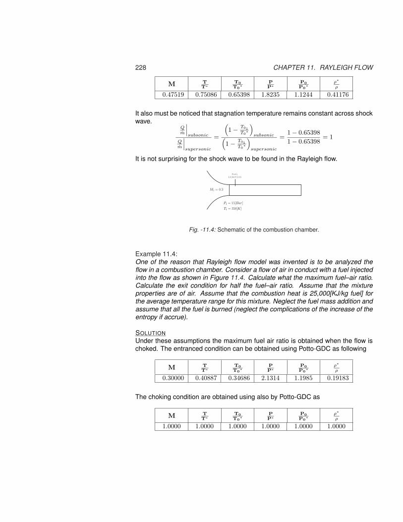
228 CHAPTER 11. RAYLEIGH FLOW
M TT∗
T0
T0∗
PP∗
P0
P0∗
ρ∗
ρ
0.47519 0.75086 0.65398 1.8235 1.1244 0.41176
It also must be noticed that stagnation temperature remains constant across shockwave.
Qm
∣∣∣subsonic
Qm
∣∣∣supersonic
=
(1− T01
T0∗
)subsonic(
1− T01T0∗
)supersonic
=1− 0.653981− 0.65398
= 1
It is not surprising for the shock wave to be found in the Rayleigh flow.
P1 = 15[Bar]
T1 = 350[K]
Fuelinjection
M1 = 0.3
Fig. -11.4: Schematic of the combustion chamber.
Example 11.4:One of the reason that Rayleigh flow model was invented is to be analyzed theflow in a combustion chamber. Consider a flow of air in conduct with a fuel injectedinto the flow as shown in Figure 11.4. Calculate what the maximum fuel–air ratio.Calculate the exit condition for half the fuel–air ratio. Assume that the mixtureproperties are of air. Assume that the combustion heat is 25,000[KJ/kg fuel] forthe average temperature range for this mixture. Neglect the fuel mass addition andassume that all the fuel is burned (neglect the complications of the increase of theentropy if accrue).
SOLUTIONUnder these assumptions the maximum fuel air ratio is obtained when the flow ischoked. The entranced condition can be obtained using Potto-GDC as following
M TT∗
T0
T0∗
PP∗
P0
P0∗
ρ∗
ρ
0.30000 0.40887 0.34686 2.1314 1.1985 0.19183
The choking condition are obtained using also by Potto-GDC as
M TT∗
T0
T0∗
PP∗
P0
P0∗
ρ∗
ρ
1.0000 1.0000 1.0000 1.0000 1.0000 1.0000

11.4. EXAMPLES FOR RAYLEIGH FLOW 229
And the isentropic relationships for Mach 0.3 are
M TT0
ρρ0
AA?
PP0
A×PA∗×P0
FF∗
0.30000 0.98232 0.95638 2.0351 0.93947 1.9119 0.89699
The maximum fuel-air can be obtained by finding the heat per unit mass.
Q
m=
Q
m= Cp (T02 − T01) = CpT1
(1− T01
T ∗
)
Q
m= 1.04× 350/0.98232× (1− 0.34686) ∼ 242.022[kJ/kg]
The fuel–air mass ratio has to be
mfuel
mair=
needed heatcombustion heat
=242.02225, 000
∼ 0.0097[kg fuel/kg air]
If only half of the fuel is supplied then the exit temperature is
T02 =Q
mCp+ T01 =
0.5× 242.0221.04
+ 350/0.98232 ∼ 472.656[K]
The exit Mach number can be determined from the exit stagnation temperature asfollowing:
T2
T ∗=
T01
T0∗
T02
T01
The last temperature ratio can be calculated from the value of the temperatures
T2
T ∗= 0.34686× 472.656
350/0.98232∼ 0.47685
The Mach number can be obtained from a Rayleigh table or using Potto-GDC
M TT∗
T0
T0∗
PP∗
P0
P0∗
ρ∗
ρ
0.33217 0.47685 0.40614 2.0789 1.1854 0.22938
It should be noted that this example is only to demonstrate how to carry the calcu-lations.
End Solution

230 CHAPTER 11. RAYLEIGH FLOW
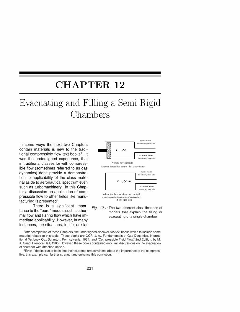
CHAPTER 12
Evacuating and Filling a Semi RigidChambers
V = f(t)Fanno model
for relatively short tube
Isothermal modelfor relatively long tube
V = f(P; et )Fanno model
for relativly short tube
Isothermal modelfor relativly long tube
Volume forced models
Volume is a function of pressure or rigid(the volume can be also a function of inertia and etc)
Semi rigid tank
External forces that control the tank volume
Fig. -12.1: The two different classifications ofmodels that explain the filling orevacuating of a single chamber
In some ways the next two Chapterscontain materials is new to the tradi-tional compressible flow text books1. Itwas the undersigned experience, thatin traditional classes for with compress-ible flow (sometimes referred to as gasdynamics) don’t provide a demonstra-tion to applicability of the class mate-rial aside to aeronautical spectrum evensuch as turbomachinery. In this Chap-ter a discussion on application of com-pressible flow to other fields like manu-facturing is presented2.
There is a significant impor-tance to the “pure” models such Isother-mal flow and Fanno flow which have im-mediate applicability. However, in manyinstances, the situations, in life, are far
1After completion of these Chapters, the undersigned discover two text books which to include somematerial related to this topic. These books are OCR, J. A., Fundamentals of Gas Dynamics, Interna-tional Textbook Co., Scranton, Pennsylvania, 1964. and “Compressible Fluid Flow,” 2nd Edition, by M.A. Saad, Prentice Hall, 1985. However, these books contained only limit discussions on the evacuationof chamber with attached nozzle.
2Even if the instructor feels that their students are convinced about the importance of the compress-ible, this example can further strength and enhance this conviction.
231

232 CHAPTER 12. EVACUATING SEMIRIGID CHAMBERS
more complicate. Combination of gas compressibility in the chamber and flow outor through a tube post a special interest and these next two Chapters are deal-ing with these topics. In the first Chapter models, were the chamber volume iscontrolled or a function of the pressure, are discussed. In the second Chapter,models, were the chamber’s volume is a function of external forces, are presented(see Figure (12.1)).
12.1 Governing Equations and AssumptionsThe process of filing or evacuating a semi flexible (semi rigid) chamber through atube is very common in engineering. For example, most car today equipped withan airbag. For instance, the models in this Chapter are suitable for study of thefilling the airbag or filling bicycle with air. The analysis is extended to include asemi rigid tank. The term semi rigid tank referred to a tank that the volume is eithercompletely rigid or is a function of the chamber’s pressure.
As it was shown in this book the most appropriate model for the flow inthe tube for a relatively fast situation is Fanno Flow. The Isothermal model is moreappropriate for cases where the tube is relatively long in–which a significant heattransfer occurs keeping the temperature almost constant. As it was shown in Chap-ter (10) the resistance, 4fL
D , should be larger than 400. Yet Isothermal flow modelis used as the limiting case.
V = f(P; et )fanno model
for relatively short tube
Isothermal modelfor a relatively long tube
A schematic of a direct connection
V = f(P; et )fanno model
for relatively short tube
Isothermal modelfor a relatively long tube
The connection is through a narrow passage
reducedconnection 1 2 1 2
Fig. -12.2: A schematic of two possible connections of the tube to a single chamber
V = f(P; t)Control volume for the evacuating case
mout
V = f(P; t)Control volume for the filling case
min
Fig. -12.3: A schematic of the control vol-umes used in this model
The Rayleigh flow model requiresthat a constant heat transfer supplied eitherby chemical reactions or otherwise. Thisauthor isn’t familiar with situations in whichRayleigh flow model is applicable. Andtherefore, at this stage, no discussion is of-fered here.
Fanno flow model is the most ap-propriate in the case where the filling andevacuating is relatively fast. In case thefilling is relatively slow (long 4fL
D than theIsothermal flow is appropriate model. Yetas it was stated before, here Isothermal flowand Fanno flow are used as limiting or bounding cases for the real flow. Addition-
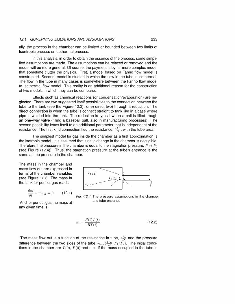
12.1. GOVERNING EQUATIONS AND ASSUMPTIONS 233
ally, the process in the chamber can be limited or bounded between two limits ofIsentropic process or Isothermal process.
In this analysis, in order to obtain the essence of the process, some simpli-fied assumptions are made. The assumptions can be relaxed or removed and themodel will be more general. Of course, the payment is by far more complex modelthat sometime clutter the physics. First, a model based on Fanno flow model isconstructed. Second, model is studied in which the flow in the tube is isothermal.The flow in the tube in many cases is somewhere between the Fanno flow modelto Isothermal flow model. This reality is an additional reason for the constructionof two models in which they can be compared.
Effects such as chemical reactions (or condensation/evaporation) are ne-glected. There are two suggested itself possibilities to the connection between thetube to the tank (see the Figure 12.2): one) direct two) through a reduction. Thedirect connection is when the tube is connect straight to tank like in a case wherepipe is welded into the tank. The reduction is typical when a ball is filled troughan one–way valve (filling a baseball ball, also in manufacturing processes). Thesecond possibility leads itself to an additional parameter that is independent of theresistance. The first kind connection tied the resistance, 4fL
D , with the tube area.
The simplest model for gas inside the chamber as a first approximation isthe isotropic model. It is assumed that kinetic change in the chamber is negligible.Therefore, the pressure in the chamber is equal to the stagnation pressure, P ≈ P0
(see Figure (12.4)). Thus, the stagnation pressure at the tube’s entrance is thesame as the pressure in the chamber.
P � P0 P1 � PU � 0 1 2
Fig. -12.4: The pressure assumptions in the chamberand tube entrance
The mass in the chamber andmass flow out are expressed interms of the chamber variables(see Figure 12.3. The mass inthe tank for perfect gas reads
dm
dt− mout = 0 (12.1)
And for perfect gas the mass atany given time is
m =P (t)V (t)RT (t)
(12.2)
The mass flow out is a function of the resistance in tube, 4fLD and the pressure
difference between the two sides of the tube mout(4fLD , P1/P2). The initial condi-
tions in the chamber are T (0), P (0) and etc. If the mass occupied in the tube is

234 CHAPTER 12. EVACUATING SEMIRIGID CHAMBERS
neglected (only for filling process) the most general equation ideal gas (12.1) reads
d
dt
m︷ ︸︸ ︷(PV
RT
)±
mout︷ ︸︸ ︷
ρ1A
U︷ ︸︸ ︷c1M1(
4fL
D,P2
P1) = 0 (12.3)
When the plus sign is for filling process and the negative sign is for evacuatingprocess.
12.2 General Model and Non-dimensionedIt is convenient to non-dimensioned the properties in chamber by dividing them bytheir initial conditions. The dimensionless properties of chamber as
T =T (t = t)T (t = 0)
(12.4a)
V =V (t = t)V (t = 0)
(12.4b)
P =P (t = t)P (t = 0)
(12.4c)
t =t
tc(12.4d)
where tc is the characteristic time of the system defined as followed
tc =V (0)
AMmax
√kRT (0))
(12.5)
The physical meaning of characteristic time, tc is the time that will take to evacuatethe chamber if the gas in the chamber was in its initial state, the flow rate was atits maximum (choking flow), and the gas was incompressible in the chamber.Utilizing these definitions (12.4) and substituting into equation (12.3) yields
P (0)V (0)tcRT (0)
d
dt
(P V
T
)±
ρ︷ ︸︸ ︷P1
RT1
P (0)T (0)
A
c(t)︷ ︸︸ ︷√kRT1T (0)MmaxM(t) = 0 (12.6)
where the following definition for the reduced Mach number is added as
M =M1(t)Mmax
(12.7)
After some rearranging equation (12.6) obtains the form
d
dt
(P V
T
)± tcAMmax
√kRT (0)
V (0)P1M1√
T1
M = 0 (12.8)

12.2. GENERAL MODEL AND NON-DIMENSIONED 235
and utilizing the definition of characteristic time, equation (12.5), and substitutinginto equation (12.8) yields
d
dt
(P V
T
)± P1M√
T1
= 0 (12.9)
Note that equation (12.9) can be modified by introducing additional parameterwhich referred to as external time, tmax
3. For cases, where the process time isimportant parameter equation (12.9) transformed to
d
dt
(P V
T
)± tmax
tc
P1M√T1
= 0 (12.10)
when P , V , T , and M are all are function of t in this case. And where t = t/tmax.It is more convenient to deal with the stagnation pressure then the actual pressureat the entrance to the tube. Utilizing the equations developed in Chapter 5 be-tween the stagnation condition, denoted without subscript, and condition in a tubedenoted with subscript 1. The ratio of P1√
T1is substituted by
P1√T1
=P√T
[1 +
k − 12
M2
]−(k+1)2(k−1)
(12.11)
It is convenient to denote
f [M ] =[1 +
k − 12
M2
]−(k+1)2(k−1)
(12.12)
Note that f [M ] is a function of the time. Utilizing the definitions (12.11) and sub-stituting equation (12.12) into equation (12.9) to be transformed into
d
dt
(P V
T
)± P M(t)f [M ]√
T= 0 (12.13)
Equation (12.13) is a first order nonlinear differential equation that can be solvedfor different initial conditions. At this stage, the author isn’t aware that there is ageneral solution for this equation4. Nevertheless, many numerical methods areavailable to solve this equation.
3This notation is used in many industrial processes where time of process referred to sometime asthe maximum time.
4To those mathematically included, find the general solution for this equation.

236 CHAPTER 12. EVACUATING SEMIRIGID CHAMBERS
12.2.1 Isentropic Process
The relationship between the pressure and the temperature in the chamber can beapproximated as isotropic and therefore
T =T (t)T (0)
=[
P (t)P (0)
] k−1k
= Pk−1
k (12.14)
The ratios can be expressed in term of the reduced pressure as followed:
P
T=
P
Pk−1
k
= P1k (12.15)
and
P√T
= Pk+12k (12.16)
So equation (12.13) is simplified into three different forms:
d
dt
(V P
1k
)± P
k+12k M(t)f [M ] = 0 (12.17a)
1k
P1−k
kdP
dtV + P
1k
dV
dt± P
k+12k M(t)f [M ] = 0 (12.17b)
VdP
dt+ kP
dV
dt± kP
3k−12k M(t)f [M ] = 0 (12.17c)
Equation (12.17) is a general equation for evacuating or filling for isentropic pro-cess in the chamber. It should be point out that, in this stage, the model in the tubecould be either Fanno flow or Isothermal flow. The situations where the chamberundergoes isentropic process but the flow in the tube is Isothermal are limited.Nevertheless, the application of this model provide some kind of a limit where toexpect when some heat transfer occurs. Note the temperature in the tube entrancecan be above or below the surrounding temperature. Simplified calculations of theentrance Mach number are described in the advance topics section.
12.2.2 Isothermal Process in The Chamber
12.2.3 A Note on the Entrance Mach number
The value of Mach number, M1 is a function of the resistance, 4fLD and the ratio
of pressure in the tank to the back pressure, PB/P1. The exit pressure, P2 is

12.3. RIGID TANK WITH NOZZLE 237
different from PB in some situations. As it was shown before, once the flow becamechoked the Mach number, M1 is only a function of the resistance, 4fL
D . Thesestatements are correct for both Fanno flow and the Isothermal flow models. Themethod outlined in Chapters ?? and 10 is appropriate for solving for entrance Machnumber, M1.Two equations must be solved for the Mach numbers at the duct entrance and exitwhen the flow is in a chokeless condition. These equations are combinations ofthe momentum and energy equations in terms of the Mach numbers. The charac-teristic equations for Fanno flow (10.50), are
4fL
D=
[4fL
D
∣∣∣∣max
]
1
−[
4fL
D
∣∣∣∣max
]
2
(12.18)
and
P2
P0(t)=
[1 +
k − 12
M22
] k1−k M1
M2
√√√√[
1 + k−12 M2
2
1 + k−12 M1
2
] k+1k−1
(12.19)
where 4fLD is defined by equation (10.49).
The solution of equations (12.18) and (12.19) for given 4fLD and Pexit
P0(t)yields the
entrance and exit Mach numbers. See advance topic about approximate solutionfor large resistance, 4fL
D or small entrance Mach number, M1.
12.3 Rigid Tank with Nozzlehe most simplest possible combination is discussed here before going trough themore complex cases A chamber is filled or evacuated by a nozzle. The gas in thechamber assumed to go an isentropic processes and flow is bounded in nozzlebetween isentropic flow and isothermal flow5. Here, it also will be assumed thatthe flow in the nozzle is either adiabatic or isothermal.
12.3.1 Adiabatic Isentropic Nozzle Attached
The mass flow out is given by either by Fliegner’s equation (5.46) or simply usecMρA∗ and equation (12.17) becomes
1k
P1−k
kdP
dt± P
k+12k (t)f [M ] = 0 (12.20)
It was utilized that V = 1 and M definition is simplified as M = 1. It can be noticedthat the characteristic time defined in equation (12.5) reduced into:
tc =V (0)
A√
kRT (0))(12.21)
5This work is suggested by Donald Katze the point out that this issue appeared in Shapiro’s BookVol 1, Chapter 4, p. 111 as a question 4.31.

238 CHAPTER 12. EVACUATING SEMIRIGID CHAMBERS
Also it can be noticed that equation (12.12) simplified into
f [M ] =[1 +
k − 12
12
]−(k+1)2(k−1)
=(
k + 12
)−(k+1)2(k−1)
(12.22)
Equation (12.20) can be simplified as
1k
(P
1−k2k
)dP ± f [m]dt = 0 (12.23)
Equation (12.23) can be integrated as∫ P
1
P1−k2k dP ±
∫ t
0
dt = 0 (12.24)
The integration limits are obtained by simply using the definitions of reduced pres-sure, at P (t = 0) = 1 and P (t = t) = P . After the integration, equation (12.24) andrearrangement becomes
P =[1±
(k − 1
2
)f [M ]t
] 2k1−k
(12.25)
Example 12.1:A chamber is connected to a main line with pressure line with a diaphragm andnozzle. The initial pressure at the chamber is 1.5[Bar] and the volume is 1.0[m3].Calculate time it requires that the pressure to reach 5[Bar] for two different noz-zles throat area of 0.001, and 0.1 [m2] when diaphragm is erupted. Assumed thestagnation temperature at the main line is the ambient of 27[◦C].
SOLUTIONThe characteristic time is
tmax =V
A∗c=
V
A∗c=
1.00.1√
1.4× 287× 300= 0.028[sec] (12.26)
And for smaller area
tmax =1.0
0.001√
1.4× 287× 300= 2.8[sec]
P =P (t)P (0)
=4.51.5
= 3.0
The time is
t = tmax
[P
1−kk − 1
] (k + 1
2
)−()
(12.27)

12.4. RAPID EVACUATING OF A RIGID TANK 239
Substituting values into equation (12.27) results
t = 0.028[3
1−1.42.8 − 1
] (2.42
)−2.40.8
= 0.013[sec] (12.28)
Filling/Evacuating The Chamber Under Upchucked Condition
The flow in the nozzle can became upchucked and it can be analytically solved.Owczarek [1964] found an analytical solution which described here.
12.3.2 Isothermal Nozzle Attached
In this case the process in nozzle is assumed to isothermal but the process in thechamber is isentropic. The temperature in the nozzle is changing because thetemperature in the chamber is changing. Yet, the differential temperature changein the chamber is slower than the temperature change in nozzle. For rigid volume,V = 1 and for isothermal nozzle T = 1 Thus, equation (12.13) is reduced into
dP
dt= ±f [M ]P = 0 (12.29)
Separating the variables and rearranging equation (12.29) converted into
∫ P
1
dP
P± f [M ]
∫ t
0
dt = 0 (12.30)
Here, f [M ] is expressed by equation (12.22). After the integration, equation(12.30) transformed into
ln P =(
k + 12
)−(k+1)2(k−1)
t
P = e
"( k+1
2 )−(k+1)2(k−1) t
#
(12.31)
12.4 Rapid evacuating of a rigid tank12.4.1 With Fanno Flow
The relative Volume, V (t) = 1, is constant and equal one for a completely rigidtank. In such case, the general equation (12.17) “shrinks” and doesn’t contain therelative volume term.
240 CHAPTER 12. EVACUATING SEMIRIGID CHAMBERS
A reasonable model for the tank is isentropic (can be replaced polytropic relation-ship) and Fanno flow are assumed for the flow in the tube. Thus, the specificgoverning equation is
dP
dt− kMf [M ]P
3k−12k = 0 (12.32)
For a choked flow the entrance Mach number to the tube is at its maximum, Mmax
and therefore M = 1. The solution of equation (12.32) is obtained by noticing thatM is not a function of time and by variables separation results in
∫ t
0
dt =∫ P
1
dP
kMf [M ]P3k−12k
=1
kMf [M ]
∫ P
1
P1−3k2k dP (12.33)
direct integration of equation (12.33) results in
t =2
(k − 1)Mf [M ]
[P
1−k2k − 1
](12.34)
It has to be realized that this is “reversed” function i.e. t is a function of P and canbe reversed for case. But for the chocked case it appears as
P =[1 +
(k − 1)Mf [M ]2
t
] 2k1−k
(12.35)
The function is drawn as shown here in Figure (12.5). The Figure (12.5) showsthat when the modified reduced pressure equal to one the reduced time is zero.The reduced time increases with decrease of the pressure in the tank.At certain point the flow becomes chokeless flow (unless the back pressure iscomplete vacuum). The transition point is denoted here as chT . Thus, equation(12.34) has to include the entrance Mach under the integration sign as
t− tchT =∫ P
PchT
1kMf [M ]
P1−3k2k dP (12.36)
For practical purposes if the flow is choked for more than 30% of the charecteristictime the choking equation can be used for the whole range, unless extra longtime or extra low pressure is calculated/needed. Further, when the flow becamechokeless the entrance Mach number does not change much from the chokingcondition.Again, for the special cases where the choked equation is not applicable the inte-gration has to be separated into zones: choked and chokeless flow regions. Andin the choke region the calculations can use the choking formula and numericalcalculations for the rest.

12.4. RAPID EVACUATING OF A RIGID TANK 241
V(t) = P (t)
V(t) = P (0)
P(t)
t
0 0.2 0.4 0.6 0.8 1.00
0.2
0.4
0.6
0.8
1.0
Fig. -12.5: The reduced time as a function of the modified reduced pressure
Example 12.2:A chamber with volume of 0.1[m3] is filled with air at pressure of 10[Bar]. Thechamber is connected with a rubber tube with f = 0.025, d = 0.01[m] and length ofL = 5.0[m]
SOLUTIONThe first parameter that calculated is 4fL
D4fLD = 5
12.4.2 Filling Process
The governing equation is
dP
dt− kMf [M ]P
3k−12k = 0 (12.37)
For a choked flow the entrance Mach number to the tube is at its maximum, Mmax
and therefore M = 1. The solution of equation (12.37) is obtained by noticing thatM is not a function of time and by variable separation results in
∫ t
0
dt =∫ P
1
dP
kMf [M ]P3k−12k
=1
kMf [M ]
∫ P
1
P1−3k2k dP (12.38)
direct integration of equation (12.38) results in
t =2
(k − 1)Mf [M ]
[P
1−k2k − 1
](12.39)

242 CHAPTER 12. EVACUATING SEMIRIGID CHAMBERS
It has to be realized that this is a reversed function. Nevertheless, with todaycomputer this should not be a problem and easily can be drawn as shown here inFigure (12.5). The Figure shows that when the modified reduced pressure equal
(k � 1)f [Mmax℄2 �P
�t
(k + 1)(3k � 1)f [Mmax℄2k2 �Por
0 0.2 0.4 0.6 0.8 1
0.2
0.4
0.6
0.8
1
0 0.2 0.4 0.6 0.8 1
0.2
0.4
0.6
0.8
1V(t) = P(t)V(t) = V(0)
Fig. -12.6: The reduced time as a function of the modified reduced pressure
to one the reduced time is zero. The reduced time increases with decrease of thepressure in the tank.At some point the flow becomes chokeless flow (unless the back pressure is acomplete vacuum). The transition point is denoted here as chT . Thus, equation(12.39) has to include the entrance Mach under the integration sign as
t− tchT =∫ P
PchT
1kMf [M ]
P1−3k2k dP (12.40)
12.4.3 The Isothermal Process
For Isothermal process, the relative temperature, T = 1. The combination of theisentropic tank and Isothermal flow in the tube is different from Fanno flow in thatthe chocking condition occurs at 1/
√k. This model is reasonably appropriated
when the chamber is insulated and not flat while the tube is relatively long and theprocess is relatively long.It has to be remembered that the chamber can undergo isothermal process. For
12.4. RAPID EVACUATING OF A RIGID TANK 243
the double isothermal (chamber and tube) the equation (12.6) reduced into
P (0)V (0)tcRT (0)
d(P V
)
dt±
ρ︷ ︸︸ ︷P1
R
P (0)T (0)
A
c(0)︷ ︸︸ ︷√kRT (0)MmaxM(t) = 0 (12.41)
12.4.4 Simple Semi Rigid Chamber
A simple relation of semi rigid chamber when the volume of the chamber is linearlyrelated to the pressure as
V (t) = aP (t) (12.42)
where a is a constant that represent the physics. This situation occurs at leastin small ranges for airbag balloon etc. The physical explanation when it occursbeyond the scope of this book. Nevertheless, a general solution is easily can beobtained similarly to rigid tank. Substituting equation (12.42) into yields
d
dt
(P
1+kk
)− P
k+12k Mf [M ] = 0 (12.43)
Carrying differentiation result in
1 + k
kP
1k
dP
dt− P
k+12k Mf [M ] = 0 (12.44)
Similarly as before, the variables are separated as
∫ t
0
dt =k
1 + k
∫ P
1
Pk−12k dP
Mf [M ](12.45)
The equation (12.45) integrated to obtain the form
t =2k2
Mf [M ](3k − 1)(1 + k)
[1− P
3k−12k
](12.46)
The physical meaning that the pressure remains larger thorough evacuating pro-cess, as results in faster reduction of the gas from the chamber.
12.4.5 The “Simple” General Case
The relationship between the pressure and the volume from the physical point ofview must be monotonous. Further, the relation must be also positive, increase ofthe pressure results in increase of the volume (as results of Hook’s law. After all, in

244 CHAPTER 12. EVACUATING SEMIRIGID CHAMBERS
the known situations to this author pressure increase results in volume decrease(at least for ideal gas.).In this analysis and previous analysis the initial effect of the chamber containerinertia is neglected. The analysis is based only on the mass conservation and ifunsteady effects are required more terms (physical quantities) have taken into ac-count. Further, it is assumed the ideal gas applied to the gas and this assumptionisn’t relaxed here.Any continuous positive monotonic function can be expressed into a polynomialfunction. However, as first approximation and simplified approach can be done bya single term with a different power as
V (t) = aPn (12.47)
When n can be any positive value including zero, 0. The physical meaning of n = 0is that the tank is rigid. In reality the value of n lays between zero to one. Whenn is approaching to zero the chamber is approaches to a rigid tank and vis versawhen the n → 1 the chamber is flexible like a balloon.There isn’t a real critical value to n. Yet, it is convenient for engineers to furtherstudy the point where the relationship between the reduced time and the reducedpressure are linear6 Value of n above it will Convex and below it concave.
d
dt
(P
1+nk−kk
)− P
k+12k Mf [M ] = 0 (12.48)
Notice that when n = 1 equation (12.49) reduced to equation (12.43).After carrying–out differentiation results
1 + nk − k
kP
1+nk−2kk
dP
dt− P
k+12k Mf [M ] = 0 (12.49)
Again, similarly as before, variables are separated and integrated as follows∫ t
0
dt =1 + nk − k
k
∫ P
1
P1+2nk−5k
2k dP
Mf [M ](12.50)
Carrying–out the integration for the initial part if exit results in
t =2k2
Mf [M ](3k − 2nk − 1)(1 + k)
[1− P
3k−2nk−12k
](12.51)
The linear condition are obtain when
3k − 2nk − 1 = 1 −→ n =3k − 2
2k(12.52)
That is just bellow 1 (n = 0.785714286) for k = 1.4.6Some suggested this border point as infinite evocation to infinite time for evacuation etc. This
undersigned is not aware situation where this indeed play important role. Therefore, it is waited to findsuch conditions before calling it as critical condition.

12.5. ADVANCE TOPICS 245
12.5 Advance TopicsThe term 4fL
D is very large for small values of the entrance Mach number whichrequires keeping many digits in the calculation. For small values of the Mach num-bers, equation (12.18) can be approximated as
4fL
D=
1k
Mexit2 −Min
2
Mexit2Min
2 (12.53)
and equation (12.19) as
Pexit
P0(t)=
Min
Mexit. (12.54)
The solution of two equations (12.53) and (12.54) yields
Min =
√√√√√1−[
Pexit
P0(t)
]2
k 4fLD
. (12.55)
This solution should used only for Min < 0.00286; otherwise equations (12.18)and (12.19) must be solved numerically.The solution of equation (12.18) and (12.19) is described in “Pressure die casting:a model of vacuum pumping” Bar-Meir, G; Eckert, E R G; Goldstein, R. J. Journalof Manufacturing Science and Engineering (USA). Vol. 118, no. 2, pp. 259-265.May 1996.

246 CHAPTER 12. EVACUATING SEMIRIGID CHAMBERS

CHAPTER 13
Evacuating/Filing Chambers underExternal Volume Control
This chapter is the second on the section dealing with filling and evacuating cham-bers. Here the model deals with the case where the volume is controlled by exter-nal forces. This kind of model is applicable to many manufacturing processes suchas die casting, extraction etc. In general the process of the displacing the gas (inmany cases air) with a liquid is a very common process. For example, in die cast-ing process liquid metal is injected to a cavity and after the cooling/solidificationperiod a part is obtained in near the final shape. One can also view the exhaustsystems of internal combustion engine in the same manner. In these processes,sometime is vital to obtain a proper evacuation of the gas (air) from the cavity.
13.1 General ModelIn this analysis, in order to obtain the essence of the process, some simplifiedassumptions are made. It simplest model of such process is when a piston isdisplacing the gas though a long tube. It assumed that no chemical reaction (orcondensation/evaporation) occur in the piston or the tube 1. It is further assumedthat the process is relatively fast. The last assumption is a appropriate assumptionin process such as die casting.
Two extreme possibilities again suggest themselves: rapid and slow pro-cesses. The two different connections, direct and through reduced area are com-bined in this analysis.
1such reaction are possible and expected to be part of process but the complicates the analysis anddo not contribute to understand to the compressibility effects.
247

248 CHAPTER 13. Evacuating under External Volume Control
13.1.1 Rapid Process
Clearly under the assumption of rapid process the heat transfer can be neglectedand Fanno flow can be assumed for the tube. The first approximation isotropicprocess describe the process inside the cylinder (see Figure (13.1)).
V = f(t)Fanno model
isontropic process 1 2
Fig. -13.1: The control volume of the “Cylinder”.
Before introducing the steps of the analysis, it is noteworthy to think aboutthe process in qualitative terms. The replacing incompressible liquid enter in thesame amount as replaced incompressible liquid. But in a compressible substancethe situation can be totally different, it is possible to obtain a situation where thatmost of the liquid entered the chamber and yet most of the replaced gas can bestill be in the chamber. Obtaining conditions where the volume of displacing liquidis equal to the displaced liquid are called the critical conditions. These critical con-ditions are very significant that they provide guidelines for the design of processes.
Obviously, the best ventilation is achieved with a large tube or area. Inmanufacture processes to minimize cost and the secondary machining such astrimming and other issues the exit area or tube has to be narrow as possible. In theexhaust system cost of large exhaust valve increase with the size and in additionreduces the strength with the size of valve2. For these reasons the optimum sizeis desired. The conflicting requirements suggest an optimum area, which is alsoindicated by experimental studies and utilized by practiced engineers.
The purpose of this analysis to yields a formula for critical/optimum ventarea in a simple form is one of the objectives of this section. The second objectiveis to provide a tool to “combine” the actual tube with the resistance in the tube,thus, eliminating the need for calculations of the gas flow in the tube to minimizethe numerical calculations.
A linear function is the simplest model that decibels changes the volume.In reality, in some situations like die casting this description is appropriate. Nev-ertheless, this model can be extended numerical in cases where more complexfunction is applied.
V (t) = V (0)[1− t
tmax
](13.1)
2After certain sizes, the possibility of crack increases.

13.1. GENERAL MODEL 249
Equation (13.1) can be non–dimensionlassed as
V (t) = 1− t (13.2)
The governing equation (12.10) that was developed in the previous Chap-ter (12) obtained the form as
[P
] 1k
{1k
V
P
dP
dt+
dV
dt
}+
tmaxMf(M)tc
[P
] k+12k = 0 (13.3)
where t = t/tmax. Notice that in this case that there are two different char-acteristic times: the “characteristic” time, tc and the “maximum” time, tmax. Thefirst characteristic time, tc is associated with the ratio of the volume and the tubecharacteristics (see equation (12.5)). The second characteristic time, tmax is as-sociated with the imposed time on the system (in this case the elapsed time of thepiston stroke).
Equation (13.3) is an nonlinear first order differential equation and can berearranged as follows
dP
k(1− tmax
tcMf [M ]P
k−12k
)P
=dt
1− t; P (0) = 1. (13.4)
Equation (13.4) is can be solved only when the flow is chocked In which case f [m]isn’t function of the time.
The solution of equation (13.4)) can be obtained by transforming and byintroducing a new variable ξ = P
k−12k and therefore P = [ξ]
2kk−1 . The reduced Pres-
sure derivative, dP = 2kk−1 [ξ](
2kk−1 )−1
dξ Utilizing this definition and there implicationreduce equation (13.4)
2 [ξ](2k
k−1 )−1dξ
(k − 1) (1−Bξ) [ξ]2k
k−1=
dt
1− t(13.5)
where B = tmax
tcMf [M ] And equation (13.5) can be further simplified as
2dξ
(k − 1) (1−Bξ) ξ=
dt
1− t(13.6)
Equation (13.6) can be integrated to obtain
2(k − 1)B
ln∣∣∣∣1−Bξ
ξ
∣∣∣∣ = − ln t (13.7)
or in a different form∣∣∣∣1−Bξ
ξ
∣∣∣∣2
(1−k)B
= t (13.8)

250 CHAPTER 13. Evacuating under External Volume Control
Now substituting to the “preferred” variable
[1− tmax
tcMf [M ]P
k−12k
Pk−12k
] 2(1−k) tmax
tcMf[M]
∣∣∣∣∣∣
1
P
= t (13.9)
The analytical solution is applicable only in the case which the flow is chokedthorough all the process. The solution is applicable to indirect connection. Thishappen when vacuum is applied outside the tube (a technique used in die castingand injection molding to improve quality by reducing porosity.). In case when theflow chokeless a numerical integration needed to be performed. In the literature,to create a direct function equation (13.4) is transformed into
dP
dt=
k(1− tmax
tcMf [M ]P
k−12k
)
1− t(13.10)
with the initial condition of
P (0) = 1 (13.11)
The analytical solution also can be approximated by a simpler equation as
P = [1− t]tmax
tc (13.12)
The results for numerical evaluation in the case when cylinder is initially at anatmospheric pressure and outside tube is also at atmospheric pressure are pre-sented in Figure (13.2). In this case only some part of the flow is choked (the laterpart). The results of a choked case are presented in Figure (13.3) in which outsidetube condition is in vacuum. These Figures (13.2) and 13.3 demonstrate the im-portance of the ratio of tmax
tc. When tmax
tc> 1 the pressure increases significantly
and verse versa. Thus, the question remains how the time ratio can be transferedto parameters that can the engineer can design in the system.
Denoting the area that creates the ratio tmax
tc= 1 as the critical area, Ac
provides the needed tool. Thus the exit area, A can be expressed as
A =A
AcAc (13.13)
The actual times ratio tmax
tc
∣∣∣@A
can be expressed as
tmax
tc
∣∣∣∣@A
=tmax
tc
∣∣∣∣@A
1︷ ︸︸ ︷tmax
tc
∣∣∣∣@Ac
(13.14)

13.1. GENERAL MODEL 251
According to equation (12.5) tc is inversely proportional to area, tc ∝ 1/A. Thus,equation (13.14) the tmax is canceled and reduced into
tmax
tc
∣∣∣∣@A
=A
Ac(13.15)
Parameters influencing the process are the area ratio, AAc
, and the frictionparameter, 4fL
D . From other detailed calculations the author thesis (later to bepublished on this www.potto.org). it was found that the influence of the parameter4fLD on the pressure development in the cylinder is quite small. The influence
is small on the residual air mass in the cylinder but larger on the Mach number,Mexit. The effects of the area ratio, A
Ac, are studied here since it is the dominant
parameter.It is important to point out the significance of the tmax
tc. This parameter rep-
resents the ratio between the filling time and the evacuating time, the time whichwould be required to evacuate the cylinder for constant mass flow rate at the max-imum Mach number when the gas temperature and pressure remain in their initialvalues. This parameter also represents the dimensionless area, A
Ac, according to
the following equationFigure (13.4) describes the pressure as a function of the dimensionless
time for various values of AAc
. The line that represents AAc
= 1 is almost straight.For large values of A
Acthe pressure increases the volume flow rate of the air until
a quasi steady state is reached. This quasi steady state is achieved when the vol-umetric air flow rate out is equal to the volume pushed by the piston. The pressureand the mass flow rate are maintained constant after this state is reached. Thepressure in this quasi steady state is a function of A
Ac. For small values of A
Acthere
is no steady state stage. When AAc
is greater than one the pressure is concave up-ward and when A
Acis less than one the pressure is concave downward as shown
in Figures (13.4), which was obtained by an integration of equation (13.9).
13.1.2 Examples
Example 13.1:Calculate the minimum required vent area for die casting process when the die vol-ume is 0.001[m3] and 4fL
D = 20. The required solidification time, tmax = 0.03[sec].
SOLUTION
13.1.3 Direct Connection
In the above analysis is applicable to indirect connection. It should be noted thatcritical area, Ac, is not function of the time. The direct connection posts more math-ematical difficulty because the critical area is not constant and time dependent.

252 CHAPTER 13. Evacuating under External Volume Control
To continue
13.2 SummaryThe analysis indicates there is a critical vent area below which the ventilation ispoor and above which the resistance to air flow is minimal. This critical area de-pends on the geometry and the filling time. The critical area also provides a meanto “combine” the actual vent area with the vent resistance for numerical simulationsof the cavity filling, taking into account the compressibility of the gas flow.

13.2. SUMMARY 253
∗`
∇
a
o
g
DimensionlessArea, A/Ac
0.00.20.51.01.22.05.0
4fLD
=
1.0
1.4
1.8
2.2
2.6
3.0
3.4
3.8
4.2
4.6
5.0
0.0 0.1 0.2 0.3 0.4 0.5 0.6 0.7 0.8 0.9 1.0
P (th)
P (0)
100.0
∗ ∗ ∗ ∗ ∗ ∗ ∗ ∗ ∗ ∗ ∗ ∗ ∗∗
∗∗
∗∗
∗∗
∗∗
∗
∗
∗
∗
∗
∗
` ` ` ` ` ` ` ` ` ``
``
``
``
``
``
`
`
`
`
`
`
`
`
`
`
∇ ∇ ∇ ∇ ∇ ∇ ∇ ∇ ∇ ∇ ∇ ∇ ∇ ∇ ∇ ∇ ∇ ∇ ∇ ∇ ∇ ∇ ∇∇
∇∇
∇∇
∇∇
∇∇
∇
∇
∇
∇
aog aog aog aog aogaog
aogaog
aog
aog
aog
a
og
a
og
a
og
a
og
a
og
a
og
a
og
a
og
a
og
a
og
a
og
a
og
a
og
a
og
a
og
a
og
a
og
a
og
a
og
a
og
a
og
a
og
a
og
a
og
a
og
a
og
a
og
∗`
∇
a
o
g
DimensionlessArea, A/Ac
0.00.20.51.01.22.05.0
4fLD
=
Dimensionless Time, th,
or, Cylinder Volume Fraction
1.0
1.4
1.8
2.2
2.6
3.0
3.4
3.8
4.2
4.6
5.0
0.0 0.1 0.2 0.3 0.4 0.5 0.6 0.7 0.8 0.9 1.0
P (th)
P (0)
5.0
∗ ∗ ∗ ∗ ∗ ∗ ∗ ∗ ∗ ∗ ∗ ∗ ∗∗
∗∗
∗∗
∗∗
∗∗
∗
∗
∗
∗
∗
∗
` ` ` ` ` ` ` ` ` ``
``
``
``
``
``
`
`
`
`
`
`
`
`
`
`
∇ ∇ ∇ ∇ ∇ ∇ ∇ ∇ ∇ ∇ ∇ ∇ ∇ ∇ ∇ ∇ ∇ ∇ ∇ ∇ ∇ ∇ ∇∇
∇∇
∇∇
∇∇
∇
∇
∇
∇
∇
∇
aog aog aog aog aogaog
aogaog
aogaog
aog
a
og
a
og
a
og
a
og
a
og
a
og
a
og
a
og
a
og
a
og
a
og
a
og
a
og
a
og
a
og
a
og
a
og
a
og
a
og
a
og
a
og
a
og
a
og
a
og
a
og
a
og
a
og
Figure b
Figure a
Fig. -13.2: The pressure ratio as a function of the dimensionless time for chokeless condition

254 CHAPTER 13. Evacuating under External Volume Control
P(t)
P(0)
DIMENSIONLESS TIME, th, or, CYLINDER VOLUME FRACTION
0
0.2
0.4
0.6
0.8
1
1.2
1.4
1.6
1.8
2
2.2
0 0.1 0.2 0.3 0.4 0.5 0.6 0.7 0.8 0.9 1
. . . . . . . . . . .
∗
×
a
0.0
0.1
0.5
1.0
1.5
4.0
.......
........
........
.......
.......
.....................................................
∗ ∗ ∗ ∗ ∗ ∗ ∗ ∗ ∗ ∗ ∗ ∗ ∗ ∗ ∗ ∗∗
∗∗
∗∗
∗∗
∗∗
∗∗
∗
∗
× × × × × × × × × × × × × × × × × × × × × × × × × × × × × × × × × × × ××
×
a
a
a
a
a
a
a
a
aa
aa
aa
aa
aa a a a a a a a a a a a a a a a a a a a a
Ac
Ahhh=
Fig. -13.3: The pressure ratio as a function of the dimensionless time for choked condition
∗`
∇
a
o
g
DimensionlessArea, A/Ac
0.00.20.51.01.22.05.0
4fLD
=
Dimensionless Time, th,
or, Cylinder Volume Fraction
1.0
1.4
1.8
2.2
2.6
3.0
3.4
3.8
4.2
4.6
5.0
0.0 0.1 0.2 0.3 0.4 0.5 0.6 0.7 0.8 0.9 1.0
P (th)
P (0)
5.0
∗ ∗ ∗ ∗ ∗ ∗ ∗ ∗ ∗ ∗ ∗ ∗ ∗∗
∗∗
∗∗
∗∗
∗∗
∗
∗
∗
∗
∗
∗
` ` ` ` ` ` ` ` ` ``
``
``
``
``
``
`
`
`
`
`
`
`
`
`
`
∇ ∇ ∇ ∇ ∇ ∇ ∇ ∇ ∇ ∇ ∇ ∇ ∇ ∇ ∇ ∇ ∇ ∇ ∇ ∇ ∇ ∇ ∇∇
∇∇
∇∇
∇∇
∇
∇
∇
∇
∇
∇
aog aog aog aog aogaog
aogaog
aogaog
aog
a
og
a
og
a
og
a
og
a
og
a
og
a
og
a
og
a
og
a
og
a
og
a
og
a
og
a
og
a
og
a
og
a
og
a
og
a
og
a
og
a
og
a
og
a
og
a
og
a
og
a
og
a
og
Fig. -13.4: The pressure ratio as a function of the dimensionless time

CHAPTER 14
Oblique Shock
14.1 Preface to Oblique Shock
�U1 U2
= 0
Fig. -14.1: A view of a straight normal shockas a limited case for oblique shock
In Chapter (6), discussion on a normalshock was presented. A normal shockis a special type of shock wave. Theother type of shock wave is the obliqueshock. In the literature oblique shock,normal shock, and Prandtl–Meyer func-tion are presented as three separateand different issues. However, one canview all these cases as three differentregions of a flow over a plate with a de-flection section. Clearly, variation of thedeflection angle from a zero (δ = 0) to apositive value results in oblique shock. Further changing the deflection angle to anegative value results in expansion waves. The common representation is doneby not showing the boundaries of these models. However, this section attempts toshow the boundaries and the limits or connections of these models1.
1In this chapter, even the whole book, a very limited discussion about reflection shocks and collisionsof weak shock, Von Neumann paradox, triple shock intersection, etc are presented. The author believesthat these issues are not relevant to most engineering students and practices. Furthermore, theseissues should not be introduced in introductory textbook of compressible flow. Those who would liketo obtain more information, should refer to J.B. Keller, “Rays, waves and asymptotics,” Bull. Am. Math.Soc. 84, 727 (1978), and E.G. Tabak and R.R. Rosales, “Focusing of weak shock waves and the VonNeuman paradox of oblique shock reflection,” Phys. Fluids 6, 1874 (1994).
255

256 CHAPTER 14. OBLIQUE SHOCK
14.2 Introduction14.2.1 Introduction to Oblique Shock
A normal shock occurs when there is a disturbance downstream which imposesa boundary condition on the flow in which the fluid/gas can react only by a sharpchange in the flow direction. As it may be recalled, normal shock occurs when awall is straight/flat (δ = 0) as shown in Figure (14.1) which occurs when somewheredownstream a disturbance2 appears. When the deflection angle is increased, thegas flow must match the boundary conditions. This matching can occur only whenthere is a discontinuity in the flow field. Thus, the direction of the flow is changedby a shock wave with an angle to the flow. This shock is commonly referred toas the oblique shock. Alternatively, as discussed in Chapter (1)3 the flow behavesas it does in a hyperbolic field. In such a case, the flow field is governed by ahyperbolic equation which deals with the case when information (like boundaryconditions) reaches from downstream only if they are within the range of influence.For information such as the disturbance (boundary condition) to reach deep intothe flow from the side requires time. During this time, the flow moves downstreamand creates an angle.
14.2.2 Introduction to Prandtl–Meyer Function
0◦
No Shockzone
ObliqueShock
θmax(k)PrandtlMeyerFunction
ν∞(k)
Fig. -14.2: The regions where oblique shock orPrandtl–Meyer function exist. Noticethat both have a maximum point anda “no solution” zone, which is aroundzero. However, Prandtl-Meyer func-tion approaches closer to a zero de-flection angle.
Decreasing the deflection angle re-sults in the same effects as before.The boundary conditions must matchthe geometry. Yet, for a negative de-flection angle (in this section’s nota-tion), the flow must be continuous.The analysis shows that the flow ve-locity must increase to achieve this re-quirement. This velocity increase isreferred to as the expansion wave. Asit will be shown in the next chapter,as opposed to oblique shock analy-sis, the increase in the upstream Machnumber determines the downstream Mach number and the “negative” deflectionangle.
It has to be pointed out that both the oblique shock and the Prandtl–Meyerfunction have a maximum point for M1 →∞. However, the maximum point for thePrandtl–Meyer function is much larger than the oblique shock by a factor of morethan 2. What accounts for the larger maximum point is the effective turning (lessentropy production) which will be explained in the next chapter (see Figure (14.2)).
2Zero velocity, pressure boundary conditions, and different inclination angle, are examples of forcesthat create shock. The zero velocity can be found in a jet flowing into a still medium of gas.
3This section is under construction and does not appear in the book yet.

14.3. OBLIQUE SHOCK 257
14.2.3 Introduction to Zero Inclination
What happens when the inclination angle is zero? Which model is correct to use?Can these two conflicting models, the oblique shock and the Prandtl–Meyer func-tion, co-exist? Or perhaps a different model better describes the physics. In somebooks and in the famous NACA report 1135 it was assumed that Mach wave andoblique shock co–occur in the same zone. Previously (see Chapter 6), it was as-sumed that normal shock occurs at the same time. In this chapter, the stabilityissue will be examined in greater detail.
14.3 Oblique Shock
Comparsion Line
Æ�U1 U2U1nU1t U2t = U1tU2nθ
θ − δ
Fig. -14.3: A typical oblique shock schematic
The shock occurs in real-ity in situations where theshock has three–dimensionaleffects. The three–dimensionaleffects of the shock make itappear as a curved plane.However, for a chosen arbi-trary accuracy it requires aspecific small area, a one–dimensional shock can beconsidered. In such a case,the change of the orientationmakes the shock considerations two–dimensional. Alternately, using an infinite(or a two–dimensional) object produces a two–dimensional shock. The two–dimensional effects occur when the flow is affected from the “side,” i.e., a changein the flow direction4.
To match the boundary conditions, the flow turns after the shock to be parallelto the inclination angle. Figure (14.3) exhibits the schematic of the oblique shock.The deflection angle, δ, is the direction of the flow after the shock (parallel to thewall). The normal shock analysis dictates that after the shock, the flow is alwayssubsonic. The total flow after the oblique shock can also be supersonic, whichdepends on the boundary layer.
Only the oblique shock’s normal component undergoes the “shock.” The tan-gent component does not change because it does not “move” across the shockline. Hence, the mass balance reads
ρ1U1n = ρ2U2n (14.1)
4The author begs for forgiveness from those who view this description as offensive (There was anunpleasant email to the author accusing him of revolt against the holy of the holies.). If you do notlike this description, please just ignore it. You can use the traditional explanation, you do not need theauthor’s permission.

258 CHAPTER 14. OBLIQUE SHOCK
The momentum equation reads
P1 + ρ1U1n2 = P2 + ρ2U2n
2 (14.2)
The momentum equation in the tangential direction yields
U1t = U2t (14.3)
The energy balance reads
CpT1 +U1n
2
2= CpT2 +
U2n2
2(14.4)
Equations (14.1), (14.2), and (14.4) are the same as the equations for normalshock with the exception that the total velocity is replaced by the perpendicularcomponents. Yet the new relationship between the upstream Mach number, thedeflection angle, δ, and the Mach angle, θ has to be solved. From the geometry itcan be observed that
tan θ =U1n
U1t
(14.5)
and
tan(θ − δ) =U2n
U2t
(14.6)
Unlike in the normal shock, here there are three possible pairs5 of solutions tothese equations. The first is referred to as the weak shock; the second is the strongshock; and the third is an impossible solution (thermodynamically)6. Experimentsand experience have shown that the common solution is the weak shock, in whichthe shock turns to a lesser extent7.
tan θ
tan(θ − δ)=
U1n
U2n
(14.7)
The above velocity–geometry equations can also be expressed in term of Machnumber, as
sin θ =M1n
M1(14.8)
5This issue is due to R. Menikoff, who raised the solution completeness issue.6The solution requires solving the entropy conservation equation. The author is not aware of “simple”
proof and a call to find a simple proof is needed.7Actually this term is used from historical reasons. The lesser extent angle is the unstable angle and
the weak angle is the middle solution. But because the literature referred to only two roots, the termlesser extent is used.

14.3. OBLIQUE SHOCK 259
sin(θ − δ) =M2n
M2(14.9)
cos θ =M1t
M1(14.10)
cos(θ − δ) =M2t
M2(14.11)
The total energy across an oblique shock wave is constant, and it followsthat the total speed of sound is constant across the (oblique) shock. It shouldbe noted that although, U1t = U2t the Mach number is M1t 6= M2t because thetemperatures on both sides of the shock are different, T1 6= T2.
As opposed to the normal shock, here angles (the second dimension) have tobe determined. The solution from this set of four equations, (14.8) through (14.11),is a function of four unknowns of M1, M2, θ, and δ. Rearranging this set utilizinggeometrical identities such as sin α = 2 sin α cos α results in
tan δ = 2 cot θ
[M1
2 sin2 θ − 1M1
2 (k + cos 2θ) + 2
](14.12)
The relationship between the properties can be determined by substitutingM1 sin θ for of M1 into the normal shock relationship, which results in
P2
P1=
2kM12 sin2 θ − (k − 1)
k + 1 (14.13)
The density and normal velocity ratio can be determined by the following equation
ρ2
ρ1=
U1n
U2n
=(k + 1)M1
2 sin2 θ
(k − 1)M12 sin2 θ + 2 (14.14)
The temperature ratio is expressed as
T2
T1=
2kM12 sin2 θ − (k − 1)
[(k − 1)M1
2 + 2]
(k + 1)2M1 (14.15)

260 CHAPTER 14. OBLIQUE SHOCK
Prandtl’s relation for oblique shock is
Un1Un2 = c2 − k − 1k + 1
Ut2 (14.16)
The Rankine–Hugoniot relations are the same as the relationship for the normalshock
P2 − P1
ρ2 − ρ1= k
P2 − P1
ρ2 − ρ1(14.17)
14.4 Solution of Mach AngleOblique shock, if orientated to a coordinate perpendicular and parallel shock planeis like a normal shock. Thus, the relationship between the properties can be de-termined by using the normal components or by utilizing the normal shock tabledeveloped earlier. One has to be careful to use the normal components of theMach numbers. The stagnation temperature contains the total velocity.
Again, the normal shock is a one–dimensional problem, thus, only one pa-rameter is required (to solve the problem). Oblique shock is a two–dimensionalproblem and two properties must be provided so a solution can be found. Prob-ably, the most useful properties are upstream Mach number, M1 and the deflec-tion angle, which create a somewhat complicated mathematical procedure, andthis will be discussed later. Other combinations of properties provide a relativelysimple mathematical treatment, and the solutions of selected pairs and selectedrelationships will be presented.
14.4.1 Upstream Mach Number, M1, and Deflection Angle, δ
Again, this set of parameters is, perhaps, the most common and natural to ex-amine. Thompson (1950) has shown that the relationship of the shock angle isobtained from the following cubic equation:
x3 + a1x2 + a2x + a3 = 0 (14.18)
where
x = sin2 θ (14.19)
and
a1 = −M12 + 2
M12 − k sin2 δ (14.20)
a2 = −2M12 + 1
M14 +
[(k + 1)2
4+
k − 1M1
2
]sin2 δ (14.21)
a3 = −cos2 δ
M14 (14.22)
14.4. SOLUTION OF MACH ANGLE 261
Equation (14.18) requires that x has to be a real and positive number toobtain a real deflection angle8. Clearly, sin θ must be positive, and the negativesign refers to the mirror image of the solution. Thus, the negative root of sin θ mustbe disregarded
The solution of a cubic equation such as (14.18) provides three roots9. Theseroots can be expressed as
x1 = −13a1 + (S + T ) (14.23)
x2 = −13a1 − 1
2(S + T ) +
12i√
3(S − T ) (14.24)
and
x3 = −13a1 − 1
2(S + T )− 1
2i√
3(S − T ) (14.25)
Where
S =3√
R +√
D, (14.26)
T =3√
R−√
D (14.27)
and where the definition of the D is
D = Q3 + R2 (14.28)
and where the definitions of Q and R are
Q =3a2 − a1
2
9(14.29)
and
R =9a1a2 − 27a3 − 2a1
3
54(14.30)
Only three roots can exist for the Mach angle, θ. From a mathematical point ofview, if D > 0, one root is real and two roots are complex. For the case D = 0, all
8 This point was pointed out by R. Menikoff. He also suggested that θ is bounded by sin−1 1/M1
and 1.9The highest power of the equation (only with integer numbers) is the number of the roots. For
example, in a quadratic equation there are two roots.

262 CHAPTER 14. OBLIQUE SHOCK
the roots are real and at least two are identical. In the last case where D < 0, allthe roots are real and unequal.
The physical meaning of the above analysis demonstrates that in the rangewhere D > 0 no solution can exist because no imaginary solution can exist10. D >0 occurs when no shock angle can be found, so that the shock normal componentis reduced to subsonic and yet parallel to the inclination angle.
Furthermore, only in some cases when D = 0 does the solution have aphysical meaning. Hence, the solution in the case of D = 0 has to be examined inthe light of other issues to determine the validity of the solution.
When D < 0, the three unique roots are reduced to two roots at least for thesteady state because thermodynamics dictates11 that. Physically, it can be shownthat the first solution(14.23), referred sometimes as a thermodynamically unstableroot, which is also related to a decrease in entropy, is “unrealistic.” Therefore, thefirst solution does not occur in reality, at least, in steady–state situations. This roothas only a mathematical meaning for steady–state analysis12.
These two roots represent two different situations. First, for the second root,the shock wave keeps the flow almost all the time as a supersonic flow and it isreferred to as the weak solution (there is a small section that the flow is subsonic).Second, the third root always turns the flow into subsonic and it is referred to as
the strong solution. It should be noted that this case is where entropy increases inthe largest amount.
In summary, if a hand moves the shock angle starting from the deflection an-gle and reaching the first angle that satisfies the boundary condition, this situationis unstable and the shock angle will jump to the second angle (root). If an addi-tional “push” is given, for example, by additional boundary conditions, the shockangle will jump to the third root13. These two angles of the strong and weak shockare stable for a two–dimensional wedge (see the appendix of this chapter for alimited discussion on the stability14).
10A call for suggestions, to explain about complex numbers and imaginary numbers should be in-cluded. Maybe insert an example where imaginary solution results in no physical solution.
11This situation is somewhat similar to a cubical body rotation. The cubical body has three symmet-rical axes which the body can rotate around. However, the body will freely rotate only around two axeswith small and large moments of inertia. The body rotation is unstable around the middle axes. Thereader can simply try it.
12There is no experimental or analytical evidence, that the author has found, showing that it is to-tally impossible. The “unstable” terms can be thermodynamically stable in unsteady case. Though,those who are dealing with rapid transient situations should be aware that this angle of oblique shockcan exist. There is no theoretical evidence that showing that in strong unsteady state this angle isunstable. The shock will initially for a very brief time transient in it and will jump from this angle to thethermodynamically stable angles.
13See the discussion on the stability. There are those who view this question not as a stability equa-tion but rather as under what conditions a strong or a weak shock will prevail.
14This material is extra and not recommended for standard undergraduate students.

14.4. SOLUTION OF MACH ANGLE 263
14.4.2 When No Oblique Shock Exist or When D > 0
Large deflection angle for given, M1
Fig. -14.4: Flow around sphericallyblunted 30◦ cone-cylinderwith Mach number 2.0. Itcan be noticed that thenormal shock, the strongshock, and the weak shockcoexist.
The first range is when the deflection anglereaches above the maximum point. For agiven upstream Mach number, M1, a changein the inclination angle requires a larger en-ergy to change the flow direction. Once, theinclination angle reaches the “maximum po-tential energy,” a change in the flow directionis no longer possible. In the alternative view,the fluid “sees” the disturbance (in this case,the wedge) in front of it and hence the normalshock occurs. Only when the fluid is away fromthe object (smaller angle) liquid “sees” the ob-ject in a different inclination angle. This differ-ent inclination angle is sometimes referred toas an imaginary angle.
The simple procedure For example, in Figure (14.4) and (14.5), the imaginaryangle is shown. The flow is far away from the object and does not “see’ the object.For example, for, M1 −→ ∞ the maximum deflection angle is calculated whenD = Q3 + R2 = 0. This can be done by evaluating the terms a1, a2, and a3 forM1 = ∞.
a1 = −1− k sin2 δ
a2 =(k + 1)2 sin2 δ
4a3 = 0
With these values the coefficients R and Q are
R =9(−)(1 + k sin2 δ)
((k+1)2 sin2 δ
4
)− (2)(−)(1 + k sin2 δ)2
54
and
Q =(1 + k sin2 δ)2
9
Solving equation (14.28) after substituting these values of Q and R provides seriesof roots from which only one root is possible. This root, in the case k = 1.4, is justabove δmax ∼ π
4 (note that the maximum is also a function of the heat ratio, k).While the above procedure provides the general solution for the three roots,
there is simplified transformation that provides solution for the strong and and weak
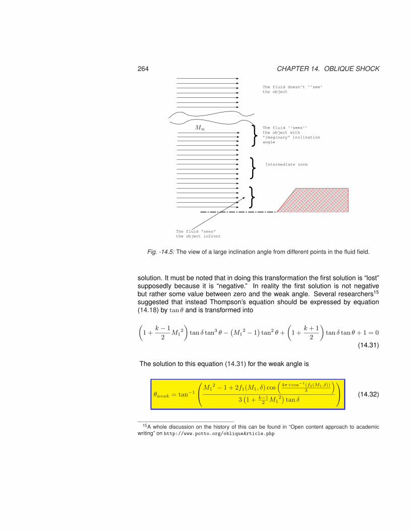
264 CHAPTER 14. OBLIQUE SHOCK
M∞
The fluid doesn’t ’’see’the object
}The fluid "sees" the object infront
The fluid ‘‘sees’’the object with "imaginary" inclinationangle
Intermediate zone}}
Fig. -14.5: The view of a large inclination angle from different points in the fluid field.
solution. It must be noted that in doing this transformation the first solution is “lost”supposedly because it is “negative.” In reality the first solution is not negativebut rather some value between zero and the weak angle. Several researchers15
suggested that instead Thompson’s equation should be expressed by equation(14.18) by tan θ and is transformed into
(1 +
k − 12
M12
)tan δ tan3 θ − (
M12 − 1
)tan2 θ +
(1 +
k + 12
)tan δ tan θ + 1 = 0
(14.31)
The solution to this equation (14.31) for the weak angle is
θweak = tan−1
M1
2 − 1 + 2f1(M1, δ) cos(
4π+cos−1(f2(M1,δ))3
)
3(1 + k−1
2 M12)tan δ
(14.32)
15A whole discussion on the history of this can be found in “Open content approach to academicwriting” on http://www.potto.org/obliqueArticle.php
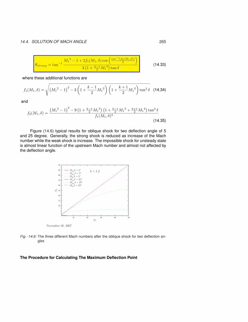
14.4. SOLUTION OF MACH ANGLE 265
θstrong = tan−1M1
2 − 1 + 2f1(M1, δ) cos(
cos−1(f2(M1,δ))3
)
3(1 + k−1
2 M12)tan δ
(14.33)
where these additional functions are
f1(M1, δ) =
√(M1
2 − 1)2 − 3
(1 +
k − 12
M12
)(1 +
k + 12
M12
)tan2 δ (14.34)
and
f2(M1, δ) =
(M1
2 − 1)3 − 9
(1 + k−1
2 M12) (
1 + k−12 M1
2 + k+12 M1
4)tan2 δ
f1(M1, δ)3(14.35)
Figure (14.6) typical results for oblique shock for two deflection angle of 5and 25 degree. Generally, the strong shock is reduced as increase of the Machnumber while the weak shock is increase. The impossible shock for unsteady stateis almost linear function of the upstream Mach number and almost not affected bythe deflection angle.
10 20 30 40 50
10
15
20
25
30
35
40
45
50
Mx
My
Mysδ = 5◦
Mywδ = 5◦
Myiδ = 5◦
Mysδ = 25◦
Mywδ = 25◦
Myiδ = 25◦
November 28, 2007
k = 1.2
Fig. -14.6: The three different Mach numbers after the oblique shock for two deflection an-gles
The Procedure for Calculating The Maximum Deflection Point

266 CHAPTER 14. OBLIQUE SHOCK
The maximum is obtained when D = 0. When the right terms defined in(14.20)-(14.21), (14.29), and (14.30) are substituted into this equation and utilizingthe trigonometrical sin2 δ + cos2 δ = 1 and other trigonometrical identities results inMaximum Deflection Mach Number’s equation in which is
M12 (k + 1) (M1n
2 + 1) = 2(kM1n4 + 2M1n
2 − 1) (14.36)
This equation and its twin equation can be obtained by an alternative procedureproposed by someone16 who suggested another way to approach this issue. Itcan be noticed that in equation (14.12), the deflection angle is a function of theMach angle and the upstream Mach number, M1. Thus, one can conclude that themaximum Mach angle is only a function of the upstream Much number, M1. Thiscan be shown mathematically by the argument that differentiating equation (14.12)and equating the results to zero creates relationship between the Mach number,M1 and the maximum Mach angle, θ. Since in that equation there appears only theheat ratio k, and Mach number, M1, θmax is a function of only these parameters.The differentiation of the equation (14.12) yields
d tan δ
dθ=
kM14 sin4 θ +
(2− (k+1)
2 M12)
M12 sin2 θ −
(1 + (k+1)
2 M12)
kM14 sin4 θ −
[(k − 1) + (k+1)2M1
2
4
]M1
2 sin2 θ − 1(14.37)
Because tan is a monotonous function, the maximum appears when θ has itsmaximum. The numerator of equation (14.37) is zero at different values of thedenominator. Thus, it is sufficient to equate the numerator to zero to obtain themaximum. The nominator produces a quadratic equation for sin2 θ and only thepositive value for sin2 θ is applied here. Thus, the sin2 θ is
sin2 θmax =−1 + k+1
4 M12 +
√(k + 1)
[1 + k−1
2 M12 +
(k+12 M1
)4]
kM12 (14.38)
Equation (14.38) should be referred to as the maximum’s equation. It should benoted that both the Maximum Mach Deflection equation and the maximum’s equa-tion lead to the same conclusion that the maximum M1n is only a function of up-stream the Mach number and the heat ratio k. It can be noticed that the MaximumDeflection Mach Number’s equation is also a quadratic equation for M1n
2. OnceM1n is found, then the Mach angle can be easily calculated by equation (14.8).To compare these two equations the simple case of Maximum for an infinite Machnumber is examined. It must be pointed out that similar procedures can also beproposed (even though it does not appear in the literature). Instead, taking thederivative with respect to θ, a derivative can be taken with respect to M1. Thus,
d tan δ
dM1= 0 (14.39)
16At first, it was seen as C. J.Chapman, English mathematician to be the creator but later an earlierversion by several months was proposed by Bernard Grossman. At this stage it is not clear who wasthe first to propose it.

14.4. SOLUTION OF MACH ANGLE 267
and then solving equation (14.39) provides a solution for Mmax.A simplified case of the Maximum Deflection Mach Number’s equation for
large Mach number becomes
M1n =
√k + 12k
M1 for M1 >> 1 (14.40)
Hence, for large Mach numbers, the Mach angle is sin θ =√
k+12k (for k=1.4), which
makes θ = 1.18 or θ = 67.79◦.With the value of θ utilizing equation (14.12), the maximum deflection angle
can be computed. Note that this procedure does not require an approximation ofM1n to be made. The general solution of equation (14.36) is
M1n =
√√(k + 1)2 M1
4 + 8 (k2 − 1) M12 + 16 (k + 1) + (k + 1) M1
2 − 4
2√
k
(14.41)
Note that Maximum Deflection Mach Number’s equation can be extended to dealwith more complicated equations of state (aside from the perfect gas model).
This typical example is for those who like mathematics.
Example 14.1:Derive the perturbation of Maximum Deflection Mach Number’s equation for thecase of a very small upstream Mach number number of the form M1 = 1 + ε. Hint,Start with equation (14.36) and neglect all the terms that are relatively small.
SOLUTIONThe solution can be done by substituting (M1 = 1 + ε) into equation (14.36) and itresults in
M1n =
√√ε(k) + ε2 + 2 ε− 3 + kε2 + 2 kε + k
4k (14.42)
where the epsilon function is
ε(k) =(k2 + 2k + 1) ε4 + (4 k2 + 8 k + 4) ε3+
(14 k2 + 12 k − 2) ε2 + (20 k2 + 8 k − 12) ε + 9 (k + 1)2 (14.43)
Now neglecting all the terms with ε results for the epsilon function in
ε(k) ∼ 9 (k + 1)2 (14.44)

268 CHAPTER 14. OBLIQUE SHOCK
And the total operation results in
M1n =
√3 (k + 1)− 3 + k
4k= 1 (14.45)
Interesting to point out that as a consequence of this assumption the maximumshock angle, θ is a normal shock. However, taking the second term results indifferent value. Taking the second term in the explanation results in
M1n =
√√√√√
9 (k + 1)2 + (20 k2 + 8 k − 12) ε− 3 + k + 2 (1 + k)ε
4k(14.46)
Note this equation (14.46) produce an un realistic value and additional terms arerequired to obtained to produce a realistic value.
The case of D ≥ 0 or 0 ≥ δ
The second range in which D > 0 is when δ < 0. Thus, first the transition linein which D = 0 has to be determined. This can be achieved by the standardmathematical procedure of equating D = 0. The analysis shows regardless of thevalue of the upstream Mach number D = 0 when δ = 0. This can be partiallydemonstrated by evaluating the terms a1, a2, and a3 for the specific value of M1 asfollowing
a1 =M1
2 + 2M1
2
a2 = −2M12 + 1
M14
a3 = − 1M1
4 (14.47)
With values presented in equations (14.47) for R and Q becoming
R =9
(M1
2+2M1
2
)(2M1
2+1M1
4
)− 27
(−1
M14
)− 2
(M1
2+2M1
2
)2
54
=9
(M1
2 + 2) (
2M12 + 1
)+ 27M1
2 − 2M12(M1
2 + 2)2
54M16 (14.48)
and
Q =3
(2M1
2+1M1
4
)−
(M1
2+2M1
2
)3
9(14.49)

14.4. SOLUTION OF MACH ANGLE 269
Substituting the values of Q and R equations (14.48) (14.49) into equation (14.28)provides the equation to be solved for δ.
3(
2M12+1
M14
)−
(M1
2+2M1
2
)3
9
3
+
[9
(M1
2 + 2) (
2M12 + 1
)+ 27M1
2 − 2M12(M1
2 + 2)2
54M16
]2
= 0 (14.50)
The author is not aware of any analytical demonstration in the literature whichshows that the solution is identical to zero for δ = 017. Nevertheless, this identitycan be demonstrated by checking several points for example, M1 = 1., 2.0,∞.Table (14.7) is provided for the following demonstration. Substitution of all theabove values into (14.28) results in D = 0.
Utilizing the symmetry and antisymmetry of the qualities of the cos and sin forδ < 0 demonstrates that D > 0 regardless of Mach number. Hence, the physicalinterpretation of this fact is that either no shock exists and the flow is without anydiscontinuity or that a normal shock exists18. Note that, in the previous case, with apositive large deflection angle, there was a transition from one kind of discontinuityto another.
XXXXXXXXXXM1
coefficientsa1 a2 a3
1.0 -3 -1 - 32
2.0 3 0 916
∞ -1 0 - 116
Fig. -14.7: The various coefficients of three differentMach numbers to demonstrate that D iszero
In the range where δ ≤ 0, thequestion is whether it is possi-ble for an oblique shock to ex-ist? The answer according tothis analysis and stability anal-ysis is no. And according tothis analysis, no Mach wavecan be generated from the wallwith zero deflection. In otherwords, the wall does not emitany signal to the flow (assum-ing zero viscosity), which con-tradicts the common approach.Nevertheless, in the literature,there are several papers suggesting zero strength Mach wave; others suggest asingular point19. The question of singular point or zero Mach wave strength areonly of mathematical interest.
17A mathematical challenge for those who like to work it out.18There are several papers that attempt to prove this point in the past. Once this analytical solu-
tion was published, this proof became trivial. But for non ideal gas (real gas) this solution is only anindication.
19See for example, paper by Rosles, Tabak, “Caustics of weak shock waves,” 206 Phys. Fluids 10 (1), January 1998.

270 CHAPTER 14. OBLIQUE SHOCK
µ1 µ2 µ3 µ∞
Fig. -14.8: The Mach waves that are sup-posed to be generated at zero in-clination.
Suppose that there is a Mach wave atthe wall at zero inclination (see Fig-ure (14.8)). Obviously, another Machwave occurs after a small distance.But because the velocity after a Machwave (even for an extremely weak shockwave) is reduced, thus, the Mach an-gle will be larger (µ2 > µ1). If the sit-uation keeps on occurring over a finitedistance, there will be a point where theMach number will be 1 and a normal shock will occur, according the common ex-planation. However, the reality is that no continuous Mach wave can occur becauseof the viscosity (boundary layer).In reality, there are imperfections in the wall and in the flow and there is the ques-tion of boundary layer. It is well known, in the engineering world, that there is nosuch thing as a perfect wall. The imperfections of the wall can be, for simplicity’ssake, assumed to be as a sinusoidal shape. For such a wall the zero inclinationchanges from small positive value to a negative value. If the Mach number is largeenough and the wall is rough enough, there will be points where a weak20 weakwill be created. On the other hand, the boundary layer covers or smooths out thebumps. With these conflicting mechanisms, both will not allow a situation of zeroinclination with emission of Mach wave. At the very extreme case, only in severalpoints (depending on the bumps) at the leading edge can a very weak shock oc-cur. Therefore, for the purpose of an introductory class, no Mach wave at zeroinclination should be assumed.Furthermore, if it was assumed that no boundary layer exists and the wall is perfect,any deviations from the zero inclination angle creates a jump from a positive angle(Mach wave) to a negative angle (expansion wave). This theoretical jump occursbecause in a Mach wave the velocity decreases while in the expansion wave thevelocity increases. Furthermore, the increase and the decrease depend on theupstream Mach number but in different directions. This jump has to be in realityeither smoothed out or has a physical meaning of jump (for example, detach normalshock). The analysis started by looking at a normal shock which occurs when thereis a zero inclination. After analysis of the oblique shock, the same conclusion mustbe reached, i.e. that the normal shock can occur at zero inclination. The analysis ofthe oblique shock suggests that the inclination angle is not the source (boundarycondition) that creates the shock. There must be another boundary condition(s)that causes the normal shock. In the light of this discussion, at least for a simpleengineering analysis, the zone in the proximity of zero inclination (small positiveand negative inclination angle) should be viewed as a zone without any changeunless the boundary conditions cause a normal shock.Nevertheless, emission of Mach wave can occur in other situations. The approxi-
20It is not a mistake, there are two “weaks.” These words mean two different things. The first “weak”means more of compression “line” while the other means the weak shock.
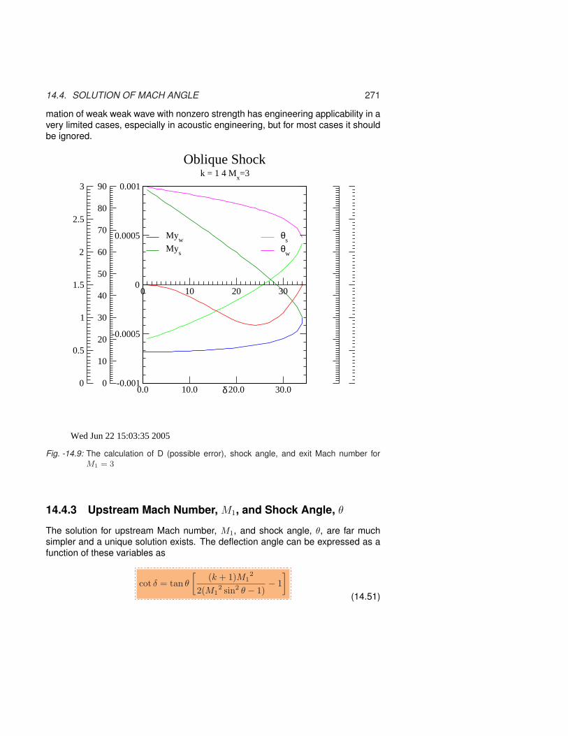
14.4. SOLUTION OF MACH ANGLE 271
mation of weak weak wave with nonzero strength has engineering applicability in avery limited cases, especially in acoustic engineering, but for most cases it shouldbe ignored.
0
0.5
1
1.5
2
2.5
3
Myw
Mys
0.0 10.0 20.0 30.00
10
20
30
40
50
60
70
80
90
θs
θw
Oblique Shockk = 1 4 M
x=3
0 10 20 30
δ-0.001
-0.0005
0
0.0005
0.001
Wed Jun 22 15:03:35 2005
Fig. -14.9: The calculation of D (possible error), shock angle, and exit Mach number forM1 = 3
14.4.3 Upstream Mach Number, M1, and Shock Angle, θ
The solution for upstream Mach number, M1, and shock angle, θ, are far muchsimpler and a unique solution exists. The deflection angle can be expressed as afunction of these variables as
cot δ = tan θ
[(k + 1)M1
2
2(M12 sin2 θ − 1)
− 1]
(14.51)

272 CHAPTER 14. OBLIQUE SHOCK
or
tan δ =2 cot θ(M1
2 sin2 θ − 1)2 + M1
2(k + 1− 2 sin2 θ)(14.52)
The pressure ratio can be expressed as
P2
P1=
2kM12 sin2 θ − (k − 1)
k + 1 (14.53)
The density ratio can be expressed as
ρ2
ρ1=
U1n
U2n
=(k + 1)M1
2 sin2 θ
(k − 1)M12 sin2 θ + 2 (14.54)
The temperature ratio expressed as
T2
T1=
c22
c12
=
(2kM1
2 sin2 θ − (k − 1)) (
(k − 1)M12 sin2 θ + 2
)
(k + 1)M12 sin2 θ (14.55)
The Mach number after the shock is
M22 sin(θ − δ) =
(k − 1)M12 sin2 θ + 2
2kM12 sin2 θ − (k − 1)
(14.56)
or explicitly
M22 =
(k + 1)2M14 sin2 θ − 4(M1
2 sin2 θ − 1)(kM12 sin2 θ + 1)(
2kM12 sin2 θ − (k − 1)
) ((k − 1)M1
2 sin2 θ + 2) (14.57)
The ratio of the total pressure can be expressed as
P02
P01
=[
(k + 1)M12 sin2 θ
(k − 1)M12 sin2 θ + 2
] kk−1
[k + 1
2kM12 sin2 θ − (k − 1)
] 1k−1
(14.58)
Even though the solution for these variables, M1 and θ, is unique, the possiblerange deflection angle, δ, is limited. Examining equation (14.51) shows that theshock angle, θ , has to be in the range of sin−1(1/M1) ≥ θ ≥ (π/2) (see Figure14.10). The range of given θ, upstream Mach number M1, is limited between ∞and
√1/ sin2 θ.
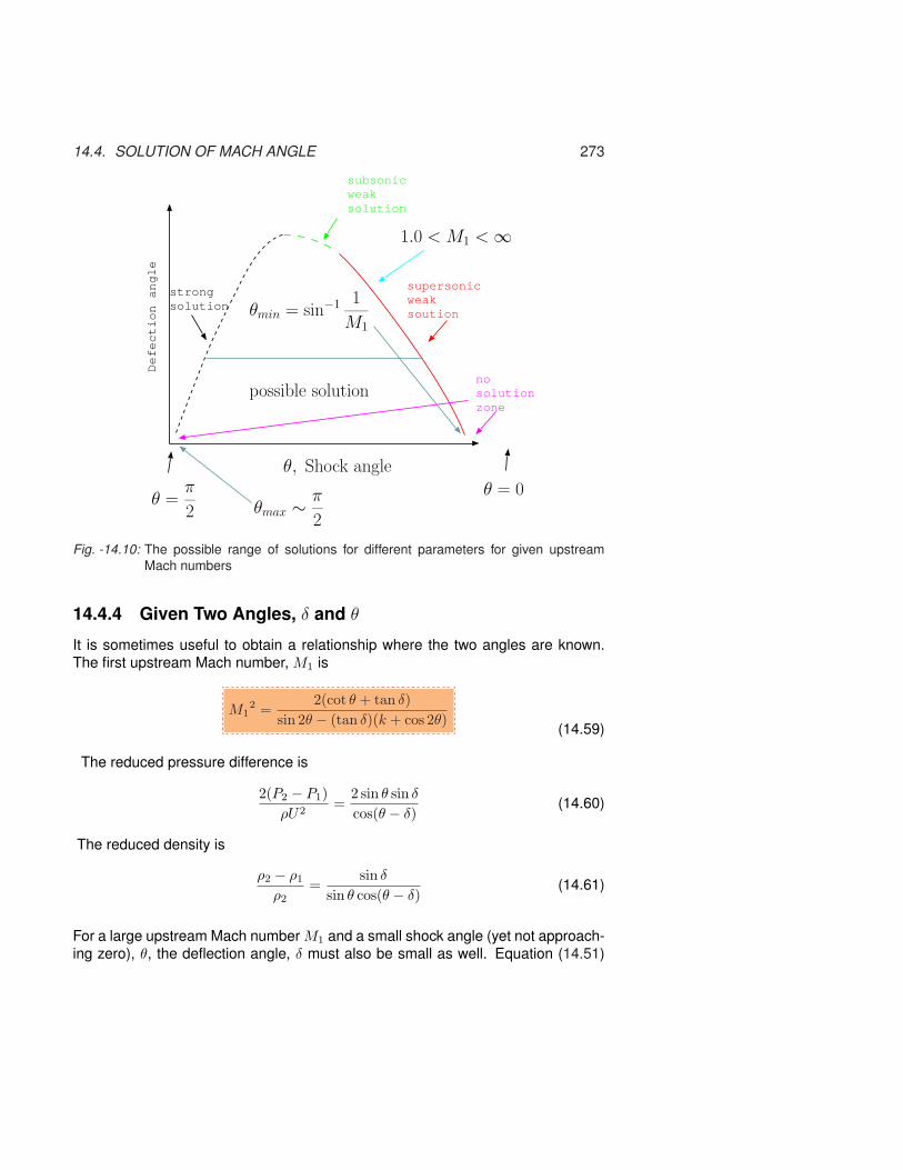
14.4. SOLUTION OF MACH ANGLE 273Defection angle
strongsolution
subsonicweaksolution
supersonicweaksoution
nosolutionzone
θmin = sin−11
M1
θ, Shock angle
θ = 0θ =
π
2
possible solution
θmax ∼
π
2
1.0 < M1 < ∞
Fig. -14.10: The possible range of solutions for different parameters for given upstreamMach numbers
14.4.4 Given Two Angles, δ and θ
It is sometimes useful to obtain a relationship where the two angles are known.The first upstream Mach number, M1 is
M12 =
2(cot θ + tan δ)sin 2θ − (tan δ)(k + cos 2θ)
(14.59)
The reduced pressure difference is
2(P2 − P1)ρU2
=2 sin θ sin δ
cos(θ − δ)(14.60)
The reduced density is
ρ2 − ρ1
ρ2=
sin δ
sin θ cos(θ − δ)(14.61)
For a large upstream Mach number M1 and a small shock angle (yet not approach-ing zero), θ, the deflection angle, δ must also be small as well. Equation (14.51)

274 CHAPTER 14. OBLIQUE SHOCK
can be simplified into
θ ∼= k + 12
δ (14.62)
The results are consistent with the initial assumption which shows that it was anappropriate assumption.
Fig. -14.11: Color-schlieren image of a two dimensional flow over a wedge. The total de-flection angel (two sides) is 20◦ and upper and lower Mach angel are ∼ 28◦ and∼ 30◦, respectively. The image show the end–effects as it has thick (not sharptransition) compare to shock over a cone. The image was taken by Gary Settlesat Gas Dynamics laboratory Penn State University.
14.4.5 Flow in a Semi–2D Shape
Example 14.2:In Figure 14.11 exhibits wedge in a supersonic flow with unknown Mach number.Examination of the Figure reveals that it is in angle of attack. 1) Calculate the Machnumber assuming that the lower and the upper Mach angles are identical and equalto ∼ 30◦ each (no angle of attack). 2) Calculate the Mach number and angle ofattack assuming that the pressure after the shock for the two oblique shocks isequal. 3) What kind are the shocks exhibits in the image? (strong, weak, unteady)4) (Open question) Is there possibilty to estimate the air stagnation temperaturefrom the information provided in the image. You can assume that spesific heats, kis a monotonic increasing function of the temperature.
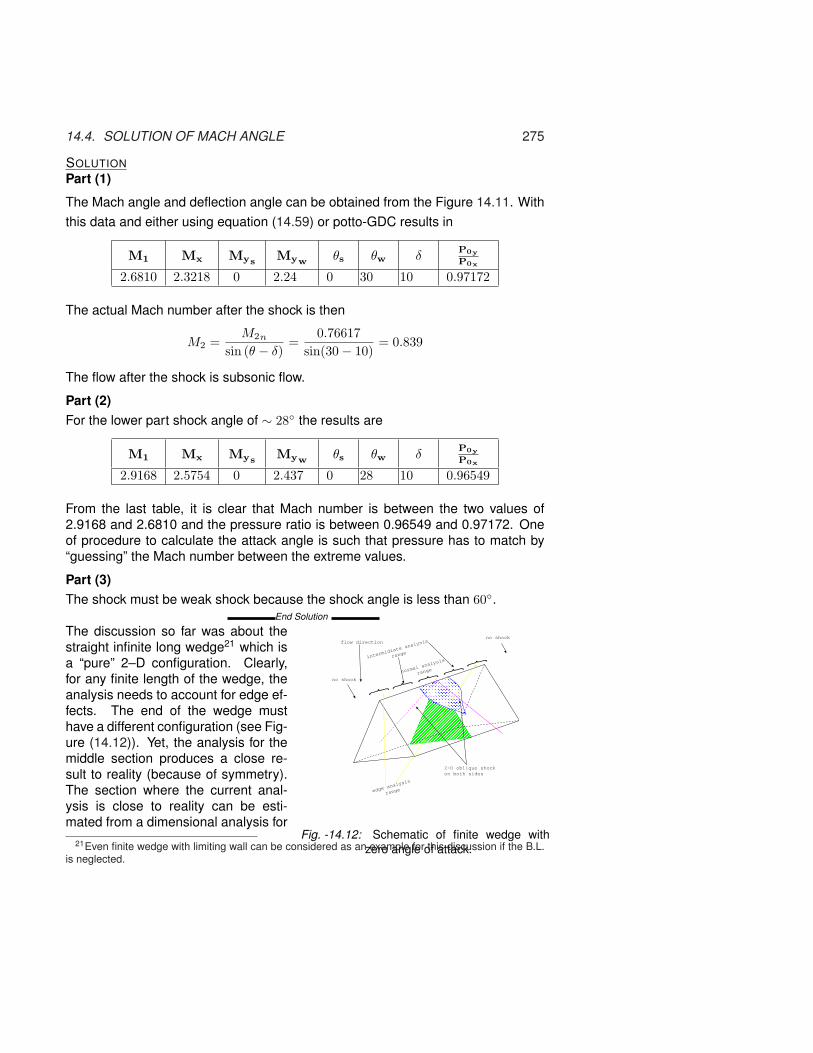
14.4. SOLUTION OF MACH ANGLE 275
SOLUTIONPart (1)
The Mach angle and deflection angle can be obtained from the Figure 14.11. Withthis data and either using equation (14.59) or potto-GDC results in
M1 Mx Mys Myw θs θw δP0y
P0x
2.6810 2.3218 0 2.24 0 30 10 0.97172
The actual Mach number after the shock is then
M2 =M2n
sin (θ − δ)=
0.76617sin(30− 10)
= 0.839
The flow after the shock is subsonic flow.
Part (2)For the lower part shock angle of ∼ 28◦ the results are
M1 Mx Mys Myw θs θw δP0y
P0x
2.9168 2.5754 0 2.437 0 28 10 0.96549
From the last table, it is clear that Mach number is between the two values of2.9168 and 2.6810 and the pressure ratio is between 0.96549 and 0.97172. Oneof procedure to calculate the attack angle is such that pressure has to match by“guessing” the Mach number between the extreme values.
Part (3)The shock must be weak shock because the shock angle is less than 60◦.
End Solution
2-D oblique shockon both sides
{normal a
nalysis
range{ {inte
rmidiate
analysi
s
range
{
{
edge ana
lysis
range
no shock
no shockflow direction
Fig. -14.12: Schematic of finite wedge withzero angle of attack.
The discussion so far was about thestraight infinite long wedge21 which isa “pure” 2–D configuration. Clearly,for any finite length of the wedge, theanalysis needs to account for edge ef-fects. The end of the wedge musthave a different configuration (see Fig-ure (14.12)). Yet, the analysis for themiddle section produces a close re-sult to reality (because of symmetry).The section where the current anal-ysis is close to reality can be esti-mated from a dimensional analysis for
21Even finite wedge with limiting wall can be considered as an example for this discussion if the B.L.is neglected.

276 CHAPTER 14. OBLIQUE SHOCK
the required accuracy or by a numer-ical method. The dimensional analy-sis shows that only the doted area tobe area where current solution can beassumed as correct22. In spite of thesmall area were the current solution can be assumed, this solution is also act asa “reality check” to any numerical analysis. The analysis also provides additionalvalue of the expected range. In Figure 14.11 shows that “shock angle” is not sharp.The thickness (into page) of the wedge is only one half times the the wedge itself23.Even for this small ratio two dimensional it provide very good results.Another geometry that can be considered as two–dimensional is the cone (somereferred to it as Taylor–Maccoll flow). Even though, the cone is a three–dimensional problem, the symmetrical nature of the cone creates a semi–2D prob-lem. In this case there are no edge effects and the geometry dictates slightlydifferent results. The mathematics is much more complicated but there are threesolutions. As before, the first solution is thermodynamical unstable. Experimentaland analytical work shows that the weak solution is the stable solution and a dis-cussion is provided in the appendix of this chapter. As opposed to the weak shock,the strong shock is unstable, at least, for steady state and no known experimentsshowing that it exist can be found in the literature. All the literature, known to theauthor, reports that only a weak shock is possible.
14.4.6 Small δ “Weak Oblique shock”
This interest in this topic is mostly from an academic point of view. It is recom-mended that this issue be skipped and the time be devoted to other issues. Theauthor is not aware of any single case in which this topic is used in real–world cal-culations. In fact, after the explicit analytical solution has been provided, studyingthis topic seems to come at the expense of other more important topics. However,the author admits that as long as there are instructors who examine their studentson this issue, it should be covered in this book.For small deflection angles, δ, and small normal upstream Mach numbers, M1 ∼1 + ε,
tan θ =1√
M12 − 1
(14.63)
... under construction.
22At this stage, dimensional analysis is not completed. The author is not aware of any such analysisin literature. The common approach is to carry out numerical analysis. In spite of recent trends, formost engineering applications, a simple tool is sufficient for limit accuracy. Additionally, the numericalworks require many times a “reality check.”
23This information is according to Gary Settles which he provided the estimate only.

14.4. SOLUTION OF MACH ANGLE 277
14.4.7 Close and Far Views of the Oblique Shock
θ
δ
Fig. -14.13: /; A local and a far view of theoblique shock.
In many cases, the close proximity viewprovides a continuous turning of the de-flection angle, δ. Yet, the far view showsa sharp transition. The traditional ap-proach to reconcile these two views isby suggesting that the far view shock isa collection of many small weak shocks(see Figure 14.13). At the local viewclose to the wall, the oblique shock is aweak “weak oblique” shock. From thefar view, the oblique shock is an accu-mulation of many small (or again weak)“weak shocks.” However, these small“shocks” are built or accumulate into alarge and abrupt change (shock). In this theory, the boundary layer (B.L.) does notenter into the calculation. In reality, the boundary layer increases the zone where acontinuous flow exists. The boundary layer reduces the upstream flow velocity andtherefore the shock does not exist at close proximity to the wall. In larger distancefrom the wall, the shock becomes possible.
14.4.8 Maximum Value of Oblique shock
The maximum values are summarized in the following Table .
Table -14.1: Table of maximum values of the oblique Shock k=1.4
Mx My δmax θmax
1.1000 0.97131 1.5152 76.27621.2000 0.95049 3.9442 71.95551.3000 0.93629 6.6621 69.36451.4000 0.92683 9.4272 67.70231.5000 0.92165 12.1127 66.56761.6000 0.91941 14.6515 65.79721.7000 0.91871 17.0119 65.30661.8000 0.91997 19.1833 64.96681.9000 0.92224 21.1675 64.75322.0000 0.92478 22.9735 64.64652.2000 0.93083 26.1028 64.60742.4000 0.93747 28.6814 64.69342.6000 0.94387 30.8137 64.84432.8000 0.94925 32.5875 65.0399

278 CHAPTER 14. OBLIQUE SHOCK
Table -14.1: Maximum values of oblique shock (continue) k=1.4
Mx My δmax θmax
3.0000 0.95435 34.0734 65.23093.2000 0.95897 35.3275 65.41443.4000 0.96335 36.3934 65.57873.6000 0.96630 37.3059 65.75933.8000 0.96942 38.0922 65.90874.0000 0.97214 38.7739 66.04645.0000 0.98183 41.1177 66.56716.0000 0.98714 42.4398 66.90207.0000 0.99047 43.2546 67.11968.0000 0.99337 43.7908 67.25039.0000 0.99440 44.1619 67.3673
10.0000 0.99559 44.4290 67.4419
It must be noted that the calculations are for the perfect gas model. In some cases,this assumption might not be sufficient and different analysis is needed. Hendersonand Menikoff24 suggested a procedure to calculate the maximum deflection anglefor arbitrary equation of state25.
14.5 Detached Shock
M < 1
M > 1
Subsonic Area
zone A
Upstream U∞
zone B
Supersoini Areazone C
Deta hment Distan eFor symmetri al bodys
θ
wea
k shoc
k
Normal Shock
Strong Shock
Fig. -14.14: The schematic for a round–tipbullet in a supersonic flow.
When the mathematical quantity D be-comes positive, for large deflection an-gle, there isn’t a physical solution to anoblique shock. Since the flow “sees” theobstacle, the only possible reaction is bya normal shock which occurs at somedistance from the body. This shock isreferred to as the detach shock. The de-tached shock’s distance from the bodyis a complex analysis and should beleft to graduate class and researchersin this area. Nevertheless, a graph anda general explanation to engineers isprovided. Even though this topic hasfew applications, some might be used incertain situations which the author isn’taware of.
24Henderson and Menikoff ”Triple Shock Entropy Theorem” Journal of Fluid Mechanics 366 (1998)pp. 179–210.
25The effect of the equation of state on the maximum and other parameters at this state is unknownat this moment and there are more works underway.
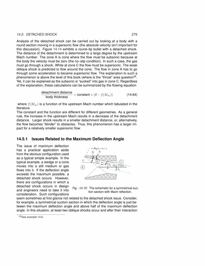
14.5. DETACHED SHOCK 279
Analysis of the detached shock can be carried out by looking at a body with around section moving in a supersonic flow (the absolute velocity isn’t important forthis discussion). Figure 14.14 exhibits a round–tip bullet with a detached shock.The distance of the detachment is determined to a large degree by the upstreamMach number. The zone A is zone where the flow must be subsonic because atthe body the velocity must be zero (the no–slip condition). In such a case, the gasmust go through a shock. While at zone C the flow must be supersonic. The weakoblique shock is predicted to flow around the cone. The flow in zone A has to gothrough some acceleration to became supersonic flow. The explanation to such aphenomenon is above the level of this book (where is the “throat” area question26.Yet, it can be explained as the subsonic is “sucked” into gas in zone C. Regardlessof the explanation, these calculations can be summarized by the flowing equation
detachment distancebody thickness
= constant× (θ − f(M∞)) (14.64)
where f(M∞) is a function of the upstream Mach number which tabulated in theliterature.The constant and the function are different for different geometries. As a generalrule, the increase in the upstream Mach results in a decrease of the detachmentdistance. Larger shock results in a smaller detachment distance, or, alternatively,the flow becomes “blinder” to obstacles. Thus, this phenomenon has a larger im-pact for a relatively smaller supersonic flow.
14.5.1 Issues Related to the Maximum Deflection Angle
oblique sho ksδ1
�2Slip Plane
θ1
θ2
δ2
U
A
B C
Fig. -14.15: The schematic for a symmetrical suc-tion section with Mach reflection.
The issue of maximum deflectionhas a practical application asidefrom the obvious configuration usedas a typical simple example. In thetypical example, a wedge or a conemoves into a still medium or gasflows into it. If the deflection angleexceeds the maximum possible, adetached shock occurs. However,there are configurations in which adetached shock occurs in designand engineers need to take it intoconsideration. Such configurationsseem sometimes at first glance not related to the detached shock issue. Consider,for example, a symmetrical suction section in which the deflection angle is just be-tween the maximum deflection angle and above half of the maximum deflectionangle. In this situation, at least two oblique shocks occur and after their interaction
26See example 14.6.
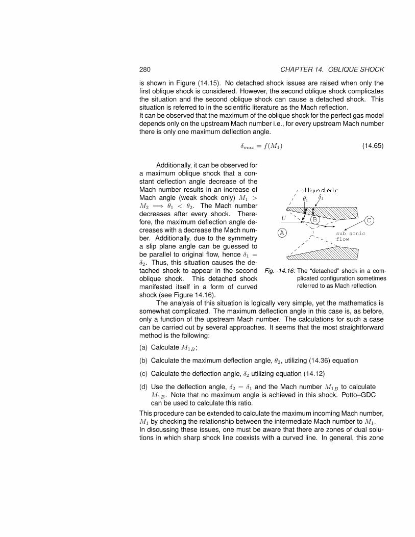
280 CHAPTER 14. OBLIQUE SHOCK
is shown in Figure (14.15). No detached shock issues are raised when only thefirst oblique shock is considered. However, the second oblique shock complicatesthe situation and the second oblique shock can cause a detached shock. Thissituation is referred to in the scientific literature as the Mach reflection.It can be observed that the maximum of the oblique shock for the perfect gas modeldepends only on the upstream Mach number i.e., for every upstream Mach numberthere is only one maximum deflection angle.
δmax = f(M1) (14.65)
oblique sho ksδ1θ1
U
A
B C
sub sonicflow
Fig. -14.16: The “detached” shock in a com-plicated configuration sometimesreferred to as Mach reflection.
Additionally, it can be observed fora maximum oblique shock that a con-stant deflection angle decrease of theMach number results in an increase ofMach angle (weak shock only) M1 >M2 =⇒ θ1 < θ2. The Mach numberdecreases after every shock. There-fore, the maximum deflection angle de-creases with a decrease the Mach num-ber. Additionally, due to the symmetrya slip plane angle can be guessed tobe parallel to original flow, hence δ1 =δ2. Thus, this situation causes the de-tached shock to appear in the secondoblique shock. This detached shockmanifested itself in a form of curvedshock (see Figure 14.16).
The analysis of this situation is logically very simple, yet the mathematics issomewhat complicated. The maximum deflection angle in this case is, as before,only a function of the upstream Mach number. The calculations for such a casecan be carried out by several approaches. It seems that the most straightforwardmethod is the following:
(a) Calculate M1B ;
(b) Calculate the maximum deflection angle, θ2, utilizing (14.36) equation
(c) Calculate the deflection angle, δ2 utilizing equation (14.12)
(d) Use the deflection angle, δ2 = δ1 and the Mach number M1B to calculateM1B . Note that no maximum angle is achieved in this shock. Potto–GDCcan be used to calculate this ratio.
This procedure can be extended to calculate the maximum incoming Mach number,M1 by checking the relationship between the intermediate Mach number to M1.In discussing these issues, one must be aware that there are zones of dual solu-tions in which sharp shock line coexists with a curved line. In general, this zone

14.5. DETACHED SHOCK 281
increases as Mach number increases. For example, at Mach 5 this zone is 8.5◦.For engineering purposes when the Mach number reaches this value, it can beignored.
14.5.2 Oblique Shock Examples
Example 14.3:Air flows at Mach number (M1) or Mx = 4 is approaching a wedge. What is themaximum wedge angle at which the oblique shock can occur? If the wedge angleis 20◦, calculate the weak, the strong Mach numbers, and the respective shockangles.
SOLUTIONThe maximum wedge angle for (Mx = 4) D has to be equal to zero. The wedgeangle that satisfies this requirement is by equation (14.28) (a side to the caseproximity of δ = 0). The maximum values are:
Mx My δmax θmax
4.0000 0.97234 38.7738 66.0407
To obtain the results of the weak and the strong solutions either utilize the equation(14.28) or the GDC which yields the following results
Mx Mys Myw θs θw δ
4.0000 0.48523 2.5686 1.4635 0.56660 0.34907
δ
θ
Fig. -14.17: Oblique shock occurs around a cone. This photo is courtesy of Dr. GrigoryToker, a Research Professor at Cuernavaco University of Mexico. According tohis measurement, the cone half angle is 15◦ and the Mach number is 2.2.

282 CHAPTER 14. OBLIQUE SHOCK
Example 14.4:A cone shown in Figure (14.17) is exposed to supersonic flow and create anoblique shock. Is the shock shown in the photo weak or strong shock? Explain.Using the geometry provided in the photo, predict at which Mach number was thephoto taken based on the assumption that the cone is a wedge.
SOLUTIONThe measurement shows that cone angle is 14.43◦ and the shock angle is 30.099◦.With given two angles the solution can be obtained by utilizing equation (14.59) orthe Potto-GDC.
M1 Mys Myw θs θw δP0y
P0x
3.2318 0.56543 2.4522 71.0143 30.0990 14.4300 0.88737
Because the flow is around the cone it must be a weak shock. Even if the conewas a wedge, the shock would be weak because the maximum (transition to astrong shock) occurs at about 60◦. Note that the Mach number is larger than theone predicted by the wedge.
0
0.5
1
1.5
2
2.5
3
My
2.0 3.0 4.0 5.0 6.0 7.0 8.0 9.0 10.0M
x
0
10
20
30
40
50
60
70
80
90
θδ
Oblique Shockk = 1 4
Thu Jun 30 15:14:53 2005
Fig. -14.18: Maximum values of the properties in an oblique shock

14.5. DETACHED SHOCK 283
14.5.3 Application of Oblique Shock
normal sho k oblique sho ks�1
�2 �3
Fig. -14.19: Two variations of inlet suction forsupersonic flow.
One of the practical applications of theoblique shock is the design of an in-let suction for a supersonic flow. It issuggested that a series of weak shocksshould replace one normal shock toincrease the efficiency (see Figure(14.19))a. Clearly, with a proper de-sign, the flow can be brought to a sub-sonic flow just below M = 1. In sucha case, there is less entropy production(less pressure loss). To illustrate the design significance of the oblique shock, thefollowing example is provided.
aIn fact, there is general proof that regardless to the equation of state (any kind of gas), the entropyis to be minimized through a series of oblique shocks rather than through a single normal shock. Fordetails see Henderson and Menikoff “Triple Shock Entropy Theorem,” Journal of Fluid Mechanics 366,(1998) pp. 179–210.
Example 14.5:The Section described in Figure 14.20 air is flowing into a suction section at M =2.0, P = 1.0[bar], and T = 17◦C. Compare the different conditions in the twodifferent configurations. Assume that only a weak shock occurs.
7◦normal sho k oblique sho ks
�1�2 7
◦
Normal shock
neglectthe detacheddistance
12 3 4
Fig. -14.20: Schematic for Example (14.5).
SOLUTIONThe first configuration is of a normal shock for which the results27 are
27The results in this example are obtained using the graphical interface of POTTO–GDC thus, noinput explanation is given. In the past the input file was given but the graphical interface it is no longerneeded.

284 CHAPTER 14. OBLIQUE SHOCK
Mx MyTy
Tx
ρy
ρx
Py
Px
P0y
P0x
2.0000 0.57735 1.6875 2.6667 4.5000 0.72087
In the oblique shock, the first angle shown is
Mx Mys Myw θs θw δP0y
P0x
2.0000 0.58974 1.7498 85.7021 36.2098 7.0000 0.99445
and the additional information by the minimal info in the Potto-GDC is
Mx Myw θw δPy
Px
Ty
Tx
P0y
P0x
2.0000 1.7498 36.2098 7.0000 1.2485 1.1931 0.99445
In the new region, the new angle is 7◦ + 7◦ with new upstream Mach number ofMx = 1.7498 resulting in
Mx Mys Myw θs θw δP0y
P0x
1.7498 0.71761 1.2346 76.9831 51.5549 14.0000 0.96524
And the additional information is
Mx Myw θw δPy
Px
Ty
Tx
P0y
P0x
1.7498 1.5088 41.8770 7.0000 1.2626 1.1853 0.99549
An oblique shock is not possible and normal shock occurs. In such a case, theresults are:
Mx MyTy
Tx
ρy
ρx
Py
Px
P0y
P0x
1.2346 0.82141 1.1497 1.4018 1.6116 0.98903
With two weak shock waves and a normal shock the total pressure loss is
P04
P01
=P04
P03
P03
P02
P02
P01
= 0.98903× 0.96524× 0.99445 = 0.9496
The static pressure ratio for the second case is
P4
P1=
P4
P3
P3
P2
P2
P1= 1.6116× 1.2626× 1.285 = 2.6147
The loss in this case is much less than in a direct normal shock. In fact, the loss inthe normal shock is above than 31% of the total pressure.

14.5. DETACHED SHOCK 285
Example 14.6:
10◦
Mys
Myw
A∗
Fig. -14.21: Schematic forExample (14.6).
A supersonic flow is approaching a very long two–dimensional bland wedge body and creates a detachedshock at Mach 3.5 (see Figure 14.21). The half wedgeangle is 10◦. What is the requited “throat” area ra-tio to achieve acceleration from the subsonic regionto the supersonic region assuming the flow is one–dimensional?
SOLUTIONThe detached shock is a normal shock and the results are
Mx MyTy
Tx
ρy
ρx
Py
Px
P0y
P0x
3.5000 0.45115 3.3151 4.2609 14.1250 0.21295
Now utilizing the isentropic relationship for k = 1.4 yields
M TT0
ρρ0
AA?
PP0
A×PA∗×P0
0.45115 0.96089 0.90506 1.4458 0.86966 1.2574
Thus the area ratio has to be 1.4458. Note that the pressure after the weak shockis irrelevant to the area ratio between the normal shock and the “throat” accordingto the standard nozzle analysis.
Example 14.7:
0 12
4
weakobliqueshock
Slip Plane
M1
P3 = P4
A
B
C
D
3
E
weakobliqueshockor expensionwave
Fig. -14.22: Schematic of two angles turn with two weakshocks.
The effects of a doublewedge are explained in thegovernment web site asshown in Figure (14.22).Adopt this description andassume that the turn of6◦ is made of two equalangles of 3◦ (see Figure14.22). Assume that thereare no boundary layers andall the shocks are weak andstraight. Perform the calcu-lation for M1 = 3.0. Findthe required angle of shockBE. Then, explain why this description has internal conflict.
SOLUTIONThe shock BD is an oblique shock with a response to a total turn of 6◦. The condi-tions for this shock are:

286 CHAPTER 14. OBLIQUE SHOCK
Mx Mys Myw θs θw δP0y
P0x
3.0000 0.48013 2.7008 87.8807 23.9356 6.0000 0.99105
The transition for shock AB is
Mx Mys Myw θs θw δP0y
P0x
3.0000 0.47641 2.8482 88.9476 21.5990 3.0000 0.99879
For the shock BC the results are
Mx Mys Myw θs θw δP0y
P0x
2.8482 0.48610 2.7049 88.8912 22.7080 3.0000 0.99894
And the isentropic relationships for M = 2.7049, 2.7008 are
M TT0
ρρ0
AA?
PP0
A×PA∗×P0
2.7049 0.40596 0.10500 3.1978 0.04263 0.136322.7008 0.40669 0.10548 3.1854 0.04290 0.13665
The combined shocks AB and BC provide the base of calculating the total pressureratio at zone 3. The total pressure ratio at zone 2 is
P02
P00
=P02
P01
P01
P00
= 0.99894× 0.99879 = 0.997731283
On the other hand, the pressure at 4 has to be
P4
P01
=P4
P04
P04
P01
= 0.04290× 0.99105 = 0.042516045
The static pressure at zone 4 and zone 3 have to match according to the govern-ment suggestion hence, the angle for BE shock which cause this pressure rationeeds to be found. To do that, check whether the pressure at 2 is above or belowor above the pressure (ratio) in zone 4.
P2
P02
=P02
P00
P2
P02
= 0.997731283× 0.04263 = 0.042436789
Since P2P02
< P4P01
a weak shock must occur to increase the static pressure (seeFigure 6.4). The increase has to be
P3/P2 = 0.042516045/0.042436789 = 1.001867743
To achieve this kind of pressure ratio the perpendicular component has to be

14.5. DETACHED SHOCK 287
Mx MyTy
Tx
ρy
ρx
Py
Px
P0y
P0x
1.0008 0.99920 1.0005 1.0013 1.0019 1.00000
The shock angle, θ can be calculated from
θ = sin−1 1.0008/2.7049 = 21.715320879◦
The deflection angle for such shock angle with Mach number is
Mx Mys Myw θs θw δP0y
P0x
2.7049 0.49525 2.7037 0.0 21.72 0.026233 1.00000
From the last calculation it is clear that the government proposed schematic of thedouble wedge is in conflict with the boundary condition. The flow in zone 3 will flowinto the wall in about 2.7◦. In reality the flow of double wedge will produce a curvedshock surface with several zones. Only when the flow is far away from the doublewedge, the flow behaves as only one theoretical angle of 6◦ exist.
Example 14.8:Calculate the flow deflection angle and other parameters downstream when theMach angle is 34◦ and P1 = 3[bar], T1 = 27◦C, and U1 = 1000m/sec. Assumek = 1.4 and R = 287J/KgK
SOLUTIONThe Mach angle of 34◦ is below maximum deflection which means that it is a weakshock. Yet, the Upstream Mach number, M1, has to be determined
M1 =U1√kRT
=1000
1.4× 287× 300= 2.88
Using this Mach number and the Mach deflection in either using the Table or thefigure or POTTO-GDC results in
Mx Mys Myw θs θw δP0y
P0x
2.8800 0.48269 2.1280 0.0 34.00 15.78 0.89127
The relationship for the temperature and pressure can be obtained by using equa-tion (14.15) and (14.13) or simply converting the M1 to perpendicular component.
M1n = M1 ∗ sin θ = 2.88 sin(34.0) = 1.61
From the Table (6.1) or GDC the following can be obtained.

288 CHAPTER 14. OBLIQUE SHOCK
Mx MyTy
Tx
ρy
ρx
Py
Px
P0y
P0x
1.6100 0.66545 1.3949 2.0485 2.8575 0.89145
The temperature ratio combined upstream temperature yield
T2 = 1.3949× 300 ∼ 418.5K
and the same for the pressure
P2 = 2.8575× 3 = 8.57[bar]
And the velocity
Un2 = Myw
√kRT = 2.128
√1.4× 287× 418.5 = 872.6[m/sec]
Example 14.9:For Mach number 2.5 and wedge with a total angle of 22◦, calculate the ratio of thestagnation pressure.
Utilizing GDC for Mach number 2.5 and the angle of 11◦ results in
Mx Mys Myw θs θw δP0y
P0x
2.5000 0.53431 2.0443 85.0995 32.8124 11.0000 0.96873
Example 14.10:What is the maximum pressure ratio that can be obtained on wedge when the gasis flowing in 2.5 Mach without any close boundaries? Would it make any differenceif the wedge was flowing into the air? If so, what is the difference?
SOLUTIONIt has to be recognized that without any other boundary condition, the shock isweak shock. For a weak shock the maximum pressure ratio is obtained at thedeflection point because it is closest to a normal shock. To obtain the maximumpoint for 2.5 Mach number, either use the Maximum Deflection Mach number’sequation or the Potto–GDC
Mx Mymax θmax δPy
Px
Ty
Tx
P0y
P0x
2.5000 0.94021 64.7822 29.7974 4.3573 2.6854 0.60027
In these calculations, Maximum Deflection Mach’s equation was used to calculatethe normal component of the upstream, then the Mach angle was calculated us-ing the geometrical relationship of θ = sin−1 M1n/M1. With these two quantities,utilizing equation (14.12) the deflection angle, δ, is obtained.

14.5. DETACHED SHOCK 289
Example 14.11:Consider the schematic shown in the following figure.
stream line
θ
δ
M1 = 4
1
2
3
Assume that the upstream Mach number is 4 and the deflection angle is δ = 15◦.Compute the pressure ratio and the temperature ratio after the second shock(sometimes referred to as the reflective shock while the first shock is called theincidental shock).
SOLUTIONThis kind of problem is essentially two wedges placed in a certain geometry. It isclear that the flow must be parallel to the wall. For the first shock, the upstreamMach number is known together with deflection angle. Utilizing the table or thePotto–GDC, the following can be obtained:
Mx Mys Myw θs θw δP0y
P0x
4.0000 0.46152 2.9290 85.5851 27.0629 15.0000 0.80382
And the additional information by using minimal information ratio button in Potto–GDC is
Mx Myw θw δPy
Px
Ty
Tx
P0y
P0x
4.0000 2.9290 27.0629 15.0000 1.7985 1.7344 0.80382
With a Mach number of M = 2.929, the second deflection angle is also 15◦. Withthese values the following can be obtained:
Mx Mys Myw θs θw δP0y
P0x
2.9290 0.51367 2.2028 84.2808 32.7822 15.0000 0.90041
and the additional information is
Mx Myw θw δPy
Px
Ty
Tx
P0y
P0x
2.9290 2.2028 32.7822 15.0000 1.6695 1.5764 0.90041
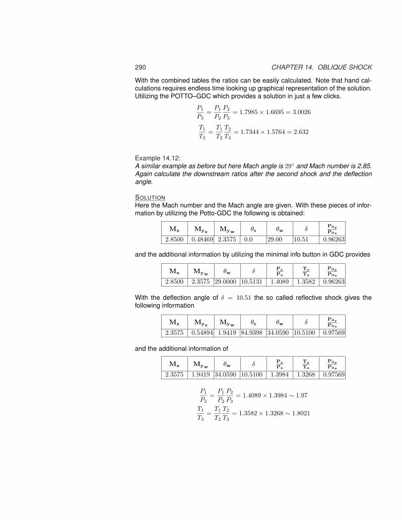
290 CHAPTER 14. OBLIQUE SHOCK
With the combined tables the ratios can be easily calculated. Note that hand cal-culations requires endless time looking up graphical representation of the solution.Utilizing the POTTO–GDC which provides a solution in just a few clicks.
P1
P3=
P1
P2
P2
P3= 1.7985× 1.6695 = 3.0026
T1
T3=
T1
T2
T2
T3= 1.7344× 1.5764 = 2.632
Example 14.12:A similar example as before but here Mach angle is 29◦ and Mach number is 2.85.Again calculate the downstream ratios after the second shock and the deflectionangle.
SOLUTIONHere the Mach number and the Mach angle are given. With these pieces of infor-mation by utilizing the Potto-GDC the following is obtained:
Mx Mys Myw θs θw δP0y
P0x
2.8500 0.48469 2.3575 0.0 29.00 10.51 0.96263
and the additional information by utilizing the minimal info button in GDC provides
Mx Myw θw δPy
Px
Ty
Tx
P0y
P0x
2.8500 2.3575 29.0000 10.5131 1.4089 1.3582 0.96263
With the deflection angle of δ = 10.51 the so called reflective shock gives thefollowing information
Mx Mys Myw θs θw δP0y
P0x
2.3575 0.54894 1.9419 84.9398 34.0590 10.5100 0.97569
and the additional information of
Mx Myw θw δPy
Px
Ty
Tx
P0y
P0x
2.3575 1.9419 34.0590 10.5100 1.3984 1.3268 0.97569
P1
P3=
P1
P2
P2
P3= 1.4089× 1.3984 ∼ 1.97
T1
T3=
T1
T2
T2
T3= 1.3582× 1.3268 ∼ 1.8021

14.5. DETACHED SHOCK 291
Example 14.13:Compare a direct normal shock to oblique shock with a normal shock. Where willthe total pressure loss (entropy) be larger? Assume that upstream Mach numberis 5 and the first oblique shock has Mach angle of 30◦. What is the deflection anglein this case?
SOLUTIONFor the normal shock the results are
Mx MyTy
Tx
ρy
ρx
Py
Px
P0y
P0x
5.0000 0.41523 5.8000 5.0000 29.0000 0.06172
While the results for the oblique shock are
Mx Mys Myw θs θw δP0y
P0x
5.0000 0.41523 3.0058 0.0 30.00 20.17 0.49901
And the additional information is
Mx Myw θw δPy
Px
Ty
Tx
P0y
P0x
5.0000 3.0058 30.0000 20.1736 2.6375 2.5141 0.49901
The normal shock that follows this oblique is
Mx MyTy
Tx
ρy
ρx
Py
Px
P0y
P0x
3.0058 0.47485 2.6858 3.8625 10.3740 0.32671
The pressure ratios of the oblique shock with normal shock is the total shock in thesecond case.
P1
P3=
P1
P2
P2
P3= 2.6375× 10.374 ∼ 27.36
T1
T3=
T1
T2
T2
T3= 2.5141× 2.6858 ∼ 6.75
Note the static pressure raised is less than the combination shocks as comparedto the normal shock but the total pressure has the opposite result.
Example 14.14:A flow in a tunnel ends up with two deflection angles from both sides (see thefollowing Figure (14.14)).

292 CHAPTER 14. OBLIQUE SHOCK
stream line
θ1
δ1
0
2
1
slip plane
φ
δ2
θ2
stream line
3
4
A
B
C
D
F
Illustration for example (14.14)
For upstream Mach number of 5 and deflection angle of 12◦ and 15◦, calculate thepressure at zones 3 and 4 based on the assumption that the slip plane is half of thedifference between the two deflection angles. Based on these calculations, explainwhether the slip angle is larger or smaller than the difference of the deflectionangle.
SOLUTIONThe first two zones immediately after are computed using the same techniquesthat were developed and discussed earlier.For the first direction of 15◦ and Mach number =5.
Mx Mys Myw θs θw δP0y
P0x
5.0000 0.43914 3.5040 86.0739 24.3217 15.0000 0.69317
And the additional conditions are
Mx Myw θw δPy
Px
Ty
Tx
P0y
P0x
5.0000 3.5040 24.3217 15.0000 1.9791 1.9238 0.69317
For the second direction of 12◦ and Mach number =5.
Mx Mys Myw θs θw δP0y
P0x
5.0000 0.43016 3.8006 86.9122 21.2845 12.0000 0.80600
And the additional conditions are
Mx Myw θw δPy
Px
Ty
Tx
P0y
P0x
5.0000 3.8006 21.2845 12.0000 1.6963 1.6625 0.80600

14.5. DETACHED SHOCK 293
The conditions in zone 4 and zone 3 have two things that are equal. They are thepressure and the velocity direction. It has to be noticed that the velocity magnitudesin zone 3 and 4 do not have to be equal. This non–continuous velocity profile canoccur in our model because it is assumed that fluid is non–viscous.If the two sides were equal because of symmetry the slip angle is also zero. It isto say, for the analysis, that only one deflection angle exist. For the two differentdeflection angles, the slip angle has two extreme cases. The first case is wherematch lower deflection angle and second is to match the higher deflection angle.In this case, it is assumed that the slip angle moves half of the angle to satisfy bothof the deflection angles (first approximation). Under this assumption the conditionsin zone 3 are solved by looking at the deflection angle of 12◦ + 1.5◦ = 13.5◦ whichresults in
Mx Mys Myw θs θw δP0y
P0x
3.5040 0.47413 2.6986 85.6819 27.6668 13.5000 0.88496
with the additional information
Mx Myw θw δPy
Px
Ty
Tx
P0y
P0x
3.5040 2.6986 27.6668 13.5000 1.6247 1.5656 0.88496
And in zone 4 the conditions are due to deflection angle of 13.5◦ and Mach 3.8006
Mx Mys Myw θs θw δP0y
P0x
3.8006 0.46259 2.9035 85.9316 26.3226 13.5000 0.86179
with the additional information
Mx Myw θw δPy
Px
Ty
Tx
P0y
P0x
3.8006 2.9035 26.3226 13.5000 1.6577 1.6038 0.86179
From these tables the pressure ratio at zone 3 and 4 can be calculated
P3
P4=
P3
P2
P2
P0
P0
P1
P1
P4= 1.6247× 1.9791
11.6963
11.6038
∼ 1.18192
To reduce the pressure ratio the deflection angle has to be reduced (rememberthat at weak weak shock almost no pressure change). Thus, the pressure at zone3 has to be reduced. To reduce the pressure the angle of slip plane has to increasefrom 1.5◦ to a larger number.

294 CHAPTER 14. OBLIQUE SHOCK
Example 14.15:The previous example gave rise to another question on the order of the deflectionangles. Consider the same values as previous analysis, will the oblique shock withfirst angle of 15◦ and then 12◦ or opposite order make a difference (M = 5)? If notwhat order will make a bigger entropy production or pressure loss? (No generalproof is needed).
SOLUTIONWaiting for the solution
14.5.4 Optimization of Suction Section Design
Under heavy construction please ignoreThe question raised is what is the optimum design for inlet suction unit?
There are several considerations that have to be taken into account besides su-personic flow which includes for example the material strength consideration andthe operation factors.
The optimum deflection angle is a function of the Mach number range inwhich the suction section is operated in. There are researchers which suggestthat the numerical work is the solution.
14.5.5 Retouch of Shock or Wave Drag
stream lines
ρ2
U2 6= 0
A2
P2
ρ1
U1 = 0
A1
P1
moving object
stationary control volume
Fig. -14.23: The diagram that explains the shock drag effect of a moving shock consideringthe oblique shock effects.
Since it was established that the common explanation is erroneous and thesteam lines are bending/changing direction when they touching the oblique shock(compare with figure (6.7)). The correct explanation is that increase of the mo-mentum into control volume is either requires increase of the force and/or resultsin acceleration of gas. So, what is the effects of the oblique shock on the ShockDrag? Figure (14.23) exhibits schematic of the oblique shock which show clearly

14.6. SUMMARY 295
that stream lines are bended. There two main points that should be discussedin this context are the additional effects and infinite/final structure. The additionaleffects are the mass start to have a vertical component. The vertical componentone hand increase the energy needed and thus increase need to move the body(larger shock drag) (note the there is a zero momentum net change for symmetricalbodies.). However, the oblique shock reduces the normal component that under-goes the shock and hence the total shock drag is reduced. The oblique shockcreates a finite amount of drag (momentum and energy lost) while a normal shockas indirectly implied in the common explanation creates de facto situation wherethe shock grows to be infinite which of course impossible. It should be noted that,oblique shock becomes less “oblique” and more parallel when other effects start tokick in.
14.6 Summary
As with normal shock, the oblique shock with upstream Mach number, M1 is al-ways greater than 1. However, in oblique, as oppose to the normal shock, thedownstream Mach number, M2 could be larger or smaller then 1. The perpendi-cular component of the downstream Mach number, M1n is always smaller than 1.Given M1 and the deflection angle, δ there could be three solutions: the first one isthe “impossible” solution in the case where D is negative, two is weak shock, andthree is strong shock. When D is positive there is no physical solution and onlynormal shock exist. When D is equal to zero, a special case is created becausethe weak and strong solutions are equal (for large deflection angle). When D > 0,for large deflection angle, there is a possibility of no two–dimensional solution re-sulting in a detached shock case.

296 CHAPTER 14. OBLIQUE SHOCK
0 10 20 30 40 50 60 70 80 90
, shock angle
5
10
15
20
25
30
35
40
45
50
55
60
- -Mach number relationship
1.051.101.151.201.31.41.51.61.71.81.92.02.22.42.62.83.03.23.43.63.84.04.5567891015800
θ
δ,defl
ection
angle
θ δ
December 4, 2007
k = 1.4
The relationship between the shock wave angle, θ and deflection angle, δ, andMach number for k=1.4. Graphs for other value can be found in separate
accompanying book for gas dynamics tables. Several additional graphs (differentk) are in a Gas Dynamics Tables by the same author.
14.7 Appendix: Oblique Shock Stability Analysis
Unstable Stable
Fig. -14.24: Typical examples of unstableand stable situations.
The stability analysis is an analysiswhich answers the question of whathappens if for some reason, the situa-tion moves away from the expected so-lution. If the answer turns out to bethat the situation will return to its origi-

14.7. APPENDIX: OBLIQUE SHOCK STABILITY ANALYSIS 297
nal state then it is referred to as the sta-ble situation. On the other hand, if theanswer is negative, then the situation isreferred to as unstable. An example to this situation, is a ball shown in the Figure(14.24). Instinctively, the stable and unstable can be recognized. There is also thesituation where the ball is between the stable and unstable situations when the ballis on a plane field which is referred to as the neutrally stable. In the same manner,the analysis for the oblique shock wave is carried out. The only difference is thathere, there are more than one parameter that can be changed, for example, theshock angle, deflection angle, and upstream Mach number. In this example onlythe weak solution is explained. The similar analysis can be applied to strong shock.Yet, in that analysis it has to be remembered that when the flow becomes subsonicthe equation changes from hyperbolic to an elliptic equation. This change compli-cates the explanation and is omitted in this section. Of course, in the analysis thestrong shock results in an elliptic solution (or region) as opposed to a hyperbolicin weak shock. As results, the discussion is more complicated but similar analysiscan be applied to the strong shock.
∆δ−
∆θ−
∆θ+
∆δ+
Fig. -14.25: The schematic of stability analysis for oblique shock.
The change in the in-clination angle resultsin a different upstreamMach number and adifferent pressure. Onthe other hand, to main-tain the same directionstream lines, the virtualchange in the deflec-tion angle has to be inthe opposite directionof the change of the shock angle. The change is determined from the solutionprovided before or from the approximation (14.62).
∆θ =k + 1
2∆δ (14.66)
Equation (14.66) can be applied for either positive, ∆θ+ or negative ∆θ− values.The pressure difference at the wall becomes a negative increment which tendsto pull the shock angle to the opposite direction. The opposite happens whenthe deflection increment becomes negative, the deflection angle becomes positivewhich increases the pressure at the wall. Thus, the weak shock is stable.Please note that this analysis doesn’t apply to the case of the close proximity ofthe δ = 0. In fact, the shock wave is unstable according to this analysis to onedirection but stable to the other direction. Yet, it must be pointed out that it doesn’tmean that the flow is unstable but rather that the model is incorrect. There isn’t anyknown experimental evidence to show that flow is unstable for δ = 0.

298 CHAPTER 14. OBLIQUE SHOCK

CHAPTER 15
Prandtl-Meyer Function
15.1 Introductionpositiveangle
maximum angle
Fig. -15.1: The definition of the angle forthe Prandtl–Meyer function.
As discussed in Chapter (14) when the de-flection turns to the opposite direction ofthe flow, the flow accelerates to match theboundary condition. The transition, as op-posed to the oblique shock, is smooth, with-out any jump in properties. Here because ofthe tradition, the deflection angle is denotedas a positive when it is away from the flow (see Figure (15.1)). In a somewhata similar concept to oblique shock there exists a “detachment” point above whichthis model breaks and another model has to be implemented. Yet, when this modelbreaks down, the flow becomes complicated, flow separation occurs, and no knownsimple model can describe the situation. As opposed to the oblique shock, thereis no limitation for the Prandtl-Meyer function to approach zero. Yet, for very smallangles, because of imperfections of the wall and the boundary layer, it has to beassumed to be insignificant.
�M 1pM 2 � 1
U�
c
Fig. -15.2: The angles of the Machline triangle
Supersonic expansion and isentropic com-pression (Prandtl-Meyer function), are an exten-sion of the Mach line concept. The Mach lineshows that a disturbance in a field of supersonicflow moves in an angle of µ, which is defined as(as shown in Figure (15.2))
µ = sin−1
(1M
)(15.1)
299
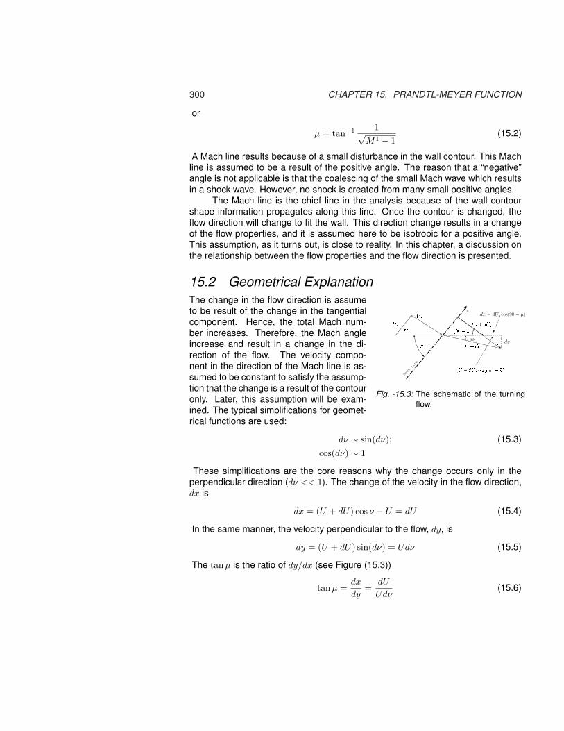
300 CHAPTER 15. PRANDTL-MEYER FUNCTION
or
µ = tan−1 1√M1 − 1
(15.2)
A Mach line results because of a small disturbance in the wall contour. This Machline is assumed to be a result of the positive angle. The reason that a “negative”angle is not applicable is that the coalescing of the small Mach wave which resultsin a shock wave. However, no shock is created from many small positive angles.
The Mach line is the chief line in the analysis because of the wall contourshape information propagates along this line. Once the contour is changed, theflow direction will change to fit the wall. This direction change results in a changeof the flow properties, and it is assumed here to be isotropic for a positive angle.This assumption, as it turns out, is close to reality. In this chapter, a discussion onthe relationship between the flow properties and the flow direction is presented.
15.2 Geometrical Explanation
� dν
UU + dU
Mach line
Ux Uy x Uy + dUy
(U + dU) os(d�)� U
dx = dUy cos(90 − µ)
(90� �) � dy
Fig. -15.3: The schematic of the turningflow.
The change in the flow direction is assumeto be result of the change in the tangentialcomponent. Hence, the total Mach num-ber increases. Therefore, the Mach angleincrease and result in a change in the di-rection of the flow. The velocity compo-nent in the direction of the Mach line is as-sumed to be constant to satisfy the assump-tion that the change is a result of the contouronly. Later, this assumption will be exam-ined. The typical simplifications for geomet-rical functions are used:
dν ∼ sin(dν); (15.3)cos(dν) ∼ 1
These simplifications are the core reasons why the change occurs only in theperpendicular direction (dν << 1). The change of the velocity in the flow direction,dx is
dx = (U + dU) cos ν − U = dU (15.4)
In the same manner, the velocity perpendicular to the flow, dy, is
dy = (U + dU) sin(dν) = Udν (15.5)
The tan µ is the ratio of dy/dx (see Figure (15.3))
tanµ =dx
dy=
dU
Udν(15.6)

15.2. GEOMETRICAL EXPLANATION 301
The ratio dU/U was shown to be
dU
U=
dM2
2M2(1 + k−1
2 M2) (15.7)
Combining equations (15.6) and (15.7) transforms it into
dν = −√
M2 − 1dM2
2M2(1 + k−1
2 M2) (15.8)
After integration of equation (15.8) becomes
ν(M) = −√
k + 1k − 1
tan−1
√k − 1k + 1
(M2 − 1) + tan−1√
(M2 − 1) + constant
(15.9)
The constant can be chosen in a such a way that ν = 0 at M = 1.
15.2.1 Alternative Approach to Governing Equations
backMachline
FrontMachline
Ur
Uθ
r
θ
Fig. -15.4: The schematic of the coordinate based on the math-ematical description.
In the previous sec-tion, a simplified ver-sion was derived basedon geometrical argu-ments. In this section,a more rigorous ex-planation is provided.It must be recognizedthat here the cylindricalcoordinates are advan-tageous because theflow turns around a sin-gle point.
For this coordinate system, the mass conservation can be written as
∂ (ρrUr)∂r
+∂ (ρUθ)
∂θ= 0 (15.10)
The momentum equations are expressed as
Ur∂Ur
∂r+
Uθ
r
∂Ur
∂θ− Uθ
2
r= −1
ρ
∂P
∂r= −c2
ρ
∂ρ
∂r(15.11)
and
Ur∂Uθ
∂r+
Uθ
r
∂Uθ
∂θ− UθUr
r= − 1
rρ
∂P
∂θ= − c2
rρ
∂ρ
∂θ(15.12)

302 CHAPTER 15. PRANDTL-MEYER FUNCTION
If the assumption is that the flow isn’t a function of the radius, r, then all thederivatives with respect to the radius will vanish. One has to remember that whenr enters to the function, like the first term in the mass equation, the derivative isn’tzero. Hence, the mass equation is reduced to
ρUr +∂ (ρUθ)
∂θ= 0 (15.13)
Equation (15.13) can be rearranged as transformed into
− 1Uθ
(Ur +
∂Uθ
∂θ
)=
1ρ
∂ρ
∂θ(15.14)
The momentum equations now obtain the form of
Uθ
r
∂Ur
∂θ− Uθ
2
r= 0
Uθ
(∂Ur
∂θ− Uθ
)= 0 (15.15)
Uθ
r
∂Uθ
∂θ− UθUr
r= − c2
rρ
∂ρ
∂θ
Uθ
(∂Uθ
∂θ− Ur
)= −c2
ρ
∂ρ
∂θ(15.16)
Substituting the term 1ρ
∂ρ∂θ from equation (15.14) into equation (15.16) results in
Uθ
(∂Uθ
∂θ− Ur
)=
c2
Uθ
(Ur +
∂Uθ
∂θ
)(15.17)
or
Uθ2
(Ur +
∂Uθ
∂θ
)= c2
(Ur +
∂Uθ
∂θ
)(15.18)
And an additional rearrangement results in
(c2 − Uθ
2) (
Ur +∂Uθ
∂θ
)= 0 (15.19)
From equation (15.19) it follows that
Uθ = c (15.20)
It is remarkable that the tangential velocity at every turn is at the speed of sound!It must be pointed out that the total velocity isn’t at the speed of sound, but only

15.2. GEOMETRICAL EXPLANATION 303
the tangential component. In fact, based on the definition of the Mach angle, thecomponent shown in Figure (15.3) under Uy is equal to the speed of sound, M = 1.
After some additional rearrangement, equation (15.15) becomes
Uθ
r
(∂Ur
∂θ− Uθ
)= 0 (15.21)
If r isn’t approaching infinity, ∞ and since Uθ 6= 0 leads to
∂Ur
∂θ= Uθ (15.22)
In the literature, these results are associated with the characteristic line. Thisanalysis can be also applied to the same equation when they are normalized byMach number. However, the non–dimensionalization can be applied at this stageas well.
The energy equation for any point on a stream line is
h(θ) +Uθ
2 + Ur2
2= h0 (15.23)
Enthalpy in perfect gas with a constant specific heat, k, is
h(θ) = CpT = CpR
RT =
1(k − 1)
c(θ)2︷ ︸︸ ︷k︷︸︸︷
Cp
CvRT =
c2
k − 1(15.24)
and substituting this equality, equation (15.24), into equation (15.23) results in
c2
k − 1+
Uθ2 + Ur
2
2= h0 (15.25)
Utilizing equation (15.20) for the speed of sound and substituting equation (15.22)which is the radial velocity transforms equation (15.25) into
(∂Ur
∂θ
)2
k − 1+
(∂Ur
∂θ
)2+ Ur
2
2= h0 (15.26)
After some rearrangement, equation (15.26) becomes
k + 1k − 1
(∂Ur
∂θ
)2
+ Ur2 = 2h0 (15.27)
Note that Ur must be positive. The solution of the differential equation (15.27)incorporating the constant becomes
Ur =√
2h0 sin
(θ
√k − 1k + 1
)(15.28)

304 CHAPTER 15. PRANDTL-MEYER FUNCTION
which satisfies equation (15.27) because sin2 θ+cos2 θ = 1. The arbitrary constantin equation (15.28) is chosen such that Ur(θ = 0) = 0. The tangential velocityobtains the form
Uθ = c =∂Ur
∂θ=
√k − 1k + 1
√2 h0 cos
(θ
√k − 1k + 1
)(15.29)
The Mach number in the turning area is
M2 =Uθ
2 + Ur2
c2=
Uθ2 + Ur
2
Uθ2 = 1 +
(Ur
Uθ
)2
(15.30)
Now utilizing the expression that was obtained for Ur and Uθ equations (15.29)and (15.28) results for the Mach number is
M2 = 1 +k + 1k − 1
tan2
(θ
√k − 1k + 1
)(15.31)
or the reverse function for θ is
θ =
√k + 1k − 1
tan−1
(√k − 1k + 1
(M2 − 1
))
(15.32)
What happens when the upstream Mach number is not 1? That is whenthe initial condition for the turning angle doesn’t start with M = 1 but is alreadyat a different angle. The upstream Mach number is denoted in this segment asMstarting. For this upstream Mach number (see Figure (15.2))
tan ν =√
Mstarting2 − 1 (15.33)
The deflection angle ν, has to match to the definition of the angle that is chosenhere (θ = 0 when M = 1), so
ν(M) = θ(M)− θ(Mstarting) (15.34)
ν(M) =
√k + 1k − 1
tan−1
(√k − 1k + 1
√M2 − 1
)− tan−1
√M2 − 1 (15.35)
These relationships are plotted in Figure (15.6).

15.3. THE MAXIMUM TURNING ANGLE 305
15.2.2 Comparison And Limitations between the Two Ap-proaches
The two models produce exactly the same results, but the assumptions for the con-struction of these models are different. In the geometrical model, the assumptionis that the velocity change in the radial direction is zero. In the rigorous model,it was assumed that radial velocity is only a function of θ. The statement for theconstruction of the geometrical model can be improved by assuming that the frameof reference is moving radially in a constant velocity.
Regardless of the assumptions that were used in the construction of thesemodels, the fact remains that there is a radial velocity at Ur(r = 0) = constant. Atthis point (r = 0) these models fail to satisfy the boundary conditions and some-thing else happens there. On top of the complication of the turning point, thequestion of boundary layer arises. For example, how did the gas accelerate toabove the speed of sound when there is no nozzle (where is the nozzle?)? Thesequestions are of interest in engineering but are beyond the scope of this book (atleast at this stage). Normally, the author recommends that this function be usedeverywhere beyond 2-4 the thickness of the boundary layer based on the upstreamlength.
In fact, analysis of design commonly used in the industry and even questionsposted to students show that many assume that the turning point can be sharp. Ata small Mach number, (1 + ε) the radial velocity is small ε. However, an increasein the Mach number can result in a very significant radial velocity. The radial ve-locity is “fed” through the reduction of the density. Aside from its close proximity toturning point, mass balance is maintained by the reduction of the density. Thus,some researchers recommend that, in many instances, the sharp point should bereplaced by a smoother transition.
15.3 The Maximum Turning AngleThe maximum turning angle is obtained when the starting Mach number is 1 andthe end Mach number approaches infinity. In this case, Prandtl–Meyer functionbecomes
ν∞ =π
2
[√k + 1k − 1
− 1
]
(15.36)
The maximum of the deflection point and the maximum turning point are onlya function of the specific heat ratios. However, the maximum turning angle is muchlarger than the maximum deflection point because the process is isentropic.
What happens when the deflection angel exceeds the maximum angle? Theflow in this case behaves as if there is almost a maximum angle and in that regionbeyond the flow will became vortex street see Figure (15.5)

306 CHAPTER 15. PRANDTL-MEYER FUNCTION
slip line
Maximumturning
Fig. -15.5: Expansion of Prandtl-Meyer function when it exceeds the maximum angle.
15.4 The Working Equations for the Prandtl-MeyerFunction
The change in the deflection angle is calculated by
ν2 − ν1 = ν(M2)− ν(M1) (15.37)
15.5 d’Alembert’s Paradox
θ1
1 2
3
4
1 2
θ1
3
4
θ2
θ2
w
Fig. -15.7: A simplified diamond shape to illustrate the su-personic d’Alembert’s Paradox
In ideal inviscid incom-pressible flows, the move-ment of body does notencounter any resistance.This result is known asd’Alembert’s Paradox, andthis paradox is examinedhere.
Supposed that a two–dimensional diamond–shapebody is stationed in a su-personic flow as shown inFigure (15.7). Again, it isassumed that the fluid is in-viscid. The net force in flow

15.5. D’ALEMBERT’S PARADOX 307
1 2 3 4 5 6 7 8 9 10Mach Number
0
20
40
60
80
100
θ
k=1.4
Prandtl-Meyer Angle
Fri Jul 8 15:39:06 2005
Fig. -15.6: The angle as a function of the Mach number
direction, the drag, is
D = 2(w
2(P2 − P4)
)= w(P2 − P4) (15.38)
It can be observed that only the area that “seems” to be by the flow wasused in expressing equation (15.38). The relation between P2 and P4 is such thatthe flow depends on the upstream Mach number, M1, and the specific heat, k.Regardless in the equation of the state of the gas, the pressure at zone 2, P2, islarger than the pressure at zone 4, P4. Thus, there is always drag when the flowis supersonic which depends on the upstream Mach number, M1, specific heat, k,and the “visible” area of the object. This drag is known in the literature as (shock)wave drag.

308 CHAPTER 15. PRANDTL-MEYER FUNCTION
15.6 Flat Body with an Angle of Attack
Slip planeα
w
ℓ
7
5
6
4
3
21
Fig. -15.8: The definition of the angle for thePrandtl–Meyer function.
Previously, the thickness of a body wasshown to have a drag. Now, a body withzero thickness but with an angle of at-tack will be examined. As opposed tothe thickness of the body, in additionto the drag, the body also obtains lift.Again, the slip condition is such that thepressure in region 5 and 7 are the same,and additionally the direction of the ve-locity must be the same. As before, themagnitude of the velocity will be differ-ent between the two regions.
15.7 Examples For Prandtl–Meyer FunctionExample 15.1:A wall is included with 20.0◦ an inclination. A flow of air with a temperature of 20◦Cand a speed of U = 450m/sec flows (see Figure 15.9). Calculate the pressurereduction ratio, and the Mach number after the bending point. If the air flows in animaginary two–dimensional tunnel with width of 0.1[m] what will the width of thisimaginary tunnel after the bend? Calculate the “fan” angle. Assume the specificheat ratio is k = 1.4.
U = 450m=se T = 20ÆC �� = 20ÆM =?�1x1 = 0:1[m℄ x2 =?�2
Fig. -15.9: The schematic of Example 15.1
SOLUTIONFirst, the initial Mach number has to be calculated (the initial speed of sound).
a =√
kRT =√
1.4 ∗ 287 ∗ 293 = 343.1m/sec

15.7. EXAMPLES FOR PRANDTL–MEYER FUNCTION 309
The Mach number is thenM =
450343.1
= 1.31
this Mach number is associated with
M ν PP0
TT0
ρρ0
µ
1.3100 6.4449 0.35603 0.74448 0.47822 52.6434
The “new” angle should be
ν2 = 6.4449 + 20 = 26.4449◦
and results in
M ν PP0
TT0
ρρ0
µ
2.0024 26.4449 0.12734 0.55497 0.22944 63.4620
Note that P01 = P02
P2
P1=
P01
P1
P2
P02
=0.127340.35603
= 0.35766
The “new” width can be calculated from the mass conservation equation.
ρ1x1M1c1 = ρ2x2M2c2 =⇒ x2 = x1ρ1
ρ2
M1
M2
√T1
T2
x2 = 0.1× 0.478220.22944
× 1.312.0024
√0.744480.55497
= 0.1579[m]
Note that the compression “fan” stream lines are note and their function can beobtain either by numerical method of going over small angle increments. The otheralternative is using the exact solution1. The expansion “fan” angle changes in theMach angle between the two sides of the bend
fan angle = 63.4 + 20.0− 52.6 = 30.8◦
Reverse the example, and this time the pressure on both sides are given and theangle has to be obtained2.
Example 15.2:Gas with k = 1.67 flows over bend (see Figure 15.2). Compute the Mach numberafter the bend, and the bend angle.
1It isn’t really different from this explanation but shown in a more mathematical form, due to Landauand friends. It will be presented in the future version. It isn’t present now because of the low priority tothis issue.
2This example is for academic understanding. There is very little with practicality in this kind ofproblem.

310 CHAPTER 15. PRANDTL-MEYER FUNCTION
M = 1:4P = 1[bar℄M =?
�1 �2P = 1:2[bar℄
Fig. -15.10: The schematic for the reversed question of example (15.2)
SOLUTIONThe Mach number is determined by satisfying the condition that the pressure down-stream are and Mach given. The relative pressure downstream can be calculatedby the relationship
P2
P02
=P2
P1
P1
P01
=1
1.2× 0.31424 = 0.2619
M ν PP0
TT0
ρρ0
µ
1.4000 7.7720 0.28418 0.60365 0.47077 54.4623
With this pressure ratio P = 0.2619 require either locking in the table or using theenclosed program.
M ν PP0
TT0
ρρ0
µ
1.4576 9.1719 0.26190 0.58419 0.44831 55.5479
For the rest of the calculation the initial condition is used. The Mach number afterthe bend is M = 1.4576. It should be noted that specific heat isn’t k = 1.4 butk = 1.67. The bend angle is
∆ν = 9.1719− 7.7720 ∼ 1.4◦
∆µ = 55.5479− 54.4623 = 1.0◦

15.8. COMBINATION OF THE OBLIQUE SHOCK AND ISENTROPIC EXPANSION311
15.8 Combination of the Oblique Shock and IsentropicExpansion
Example 15.3:Consider two–dimensional flat thin plate at an angle of attack of 4◦ and a Machnumber of 3.3. Assume that the specific heat ratio at stage is k = 1.3, calculatethe drag coefficient and lift coefficient.
SOLUTIONFor M = 3.3, the following table can be obtained:
M ν PP0
TT0
ρρ0
µ
3.3000 62.3113 0.01506 0.37972 0.03965 73.1416
With the angle of attack the region 3 will be at ν ∼ 62.31 + 4 for which the followingtable can be obtained (Potto-GDC)
M ν PP0
TT0
ρρ0
µ
3.4996 66.3100 0.01090 0.35248 0.03093 74.0528
On the other side, the oblique shock (assuming weak shock) results in
Mx Mys Myw θs θw δP0y
P0x
3.3000 0.43534 3.1115 88.9313 20.3467 4.0000 0.99676
and the additional information, by clicking on the minimal button, provides
Mx Myw θw δPy
Px
Ty
Tx
P0y
P0x
3.3000 3.1115 20.3467 4.0000 1.1157 1.1066 0.99676
The pressure ratio at point 3 is
P3
P1=
P3
P03
P03
P01
P01
P1= 0.0109× 1× 1
0.01506∼ 0.7238
The pressure ratio at point 4 is
P3
P1= 1.1157
dL =2
kP1M12 (P4−P3) cos α =
2kM1
2
(P4
P1− P3
P1
)cosα =
21.33.32
(1.1157− 0.7238) cos 4◦ ∼ .054
dd =2
kM12
(P4
P1− P3
P1
)sin α =
21.33.32
(1.1157− 0.7238) sin 4◦ ∼ .0039
This shows that on the expense of a small drag, a large lift can be obtained. Dis-cussion on the optimum design is left for the next versions.

312 CHAPTER 15. PRANDTL-MEYER FUNCTION
A∗
Aexit
Mjet1
Slip linesexpenssion
lines
β
β
Psurroundings
Fig. -15.11: Schematic of the nozzle and Prandtle–Meyer expansion.
Example 15.4:To understand the flow after a nozzle consider a flow in a nozzle shown in Figure15.4. The flow is choked and additionally the flow pressure reaches the nozzleexit above the surrounding pressure. Assume that there is an isentropic expansion(Prandtl–Meyer expansion) after the nozzle with slip lines in which there is a the-oretical angle of expansion to match the surroundings pressure with the exit. Theratio of exit area to throat area ratio is 1:3. The stagnation pressure is 1000 [kPa].The surroundings pressure is 100[kPa]. Assume that the specific heat, k = 1.3.Estimate the Mach number after the expansion.
SOLUTIONThe Mach number a the nozzle exit can be calculated using Potto-GDC whichprovides
M TT0
ρρ0
AA?
PP0
A×PA∗×P0
FF∗
1.7632 0.61661 0.29855 1.4000 0.18409 0.25773 0.57478
Thus the exit Mach number is 1.7632 and the pressure at the exit is
Pexit = P0P − exit
P − 0= 1000× 0.18409 = 184.09[kPa]
This pressure is higher than the surroundings pressure and additional expansionmust occur. This pressure ratio is associated with a expansion angle that Potto-GDC provide as
M ν PP0
TT0
ρρ0
µ
1.7632 19.6578 0.18409 0.61661 0.29855 60.4403
The need additional pressure ratio reduction is
Psurroundings
P0=
Psurroundings
Pexit
Pexit
P0=
100184.09
× 0.18409 = 0.1

15.8. COMBINATION OF THE OBLIQUE SHOCK AND ISENTROPIC EXPANSION313
Potto-GDC provides for this pressure ratio
M ν PP0
TT0
ρρ0
µ
2.1572 30.6147 0.10000 0.51795 0.19307 65.1292
The change of the angle is
∆angle = 30.6147− 19.6578 = 10.9569
Thus the angle, β isβ = 90− 10.9569 ∼ 79.0
The pressure at this point is as the surroundings. However, the stagnation pressureis the same as originally was enter the nozzle! This stagnation pressure has togo through serious of oblique shocks and Prandtl-Meyer expansion to match thesurroundings stagnation pressure.
End Solution

314 CHAPTER 15. PRANDTL-MEYER FUNCTION

APPENDIX A
Computer Program
A.1 About the ProgramThe program is written in a C++ language. This program was used to generate allthe data in this book. Some parts of the code are in FORTRAN (old code especiallyfor chapters 12 and 13 and not included here.1. The program has the base classof basic fluid mechanics and utilities functions to calculate certain properties givendata. The derived class are Fanno, isothermal, shock and others.At this stage only the source code of the program is available no binary available.This program is complied under gnu g++ in /Gnu/Linux system. As much supportas possible will be provided if it is in Linux systems. NO Support whatsoever willbe provided for any Microsoft system. In fact even PLEASE do not even try to usethis program under any Microsoft window system.
A.2 UsageTo use the program some information has to be provided. The necessary inputparameter(s), the kind of the information needed, where it has to be in a LATEXformat or not, and in many case where it is a range of parameter(s).
machV The Mach number and it is used in stagnation class
fldV The 4fLD and it is used in Fanno class isothermal class
p2p1V The pressure ratio of the two sides of the tubes
M1V Entrance Mach M1 to the tube Fanno and isothermal classes1when will be written in C++ will be add to this program.
315

316 APPENDIX A. COMPUTER PROGRAM
M1ShockV Entrance Mach M1 when expected shock to the tube Fanno and isothermalclasses
FLDShockV FLD with shock in the in Fanno class
M1fldV both M1 and 4fLD are given
M1fldP2P1V three part info P1P2
, M1 and 4fLD are given
MxV Mx or My
infoStagnation print standard (stagnation) info
infoStandard standard info for (Fanno, shock etc)
infoTube print tube side info for (Fanno, etc) including
infoShock print shock sides info
infoTubeShock print tube info shock main info
infoTubeProfile the Mach number and pressure ratio profiles
infoTubeShockLimits print tube limits with shock
To get the shock results in LATEX of Mx The following lines have to be inserted inthe end of the main function.
int isTex = yes;int isRange = no;whatInfo = infoStandard ;variableName = MxV;Mx = 2.0 ;s.makeTable(whatInfo, isRange, isTex, variableName, variableValue);
*******************************************The following stuff is the same as above/belowif you use showResults with showHeads but theinformation is setup for the latex text processing.You can just can cut and paste it in your latex file.You must use longtable style file and dcolumnstyle files.
*******************************************\setlongtables\begin{longtable}{|D..{1.4}|D..{1.4}|D..{1.4}|D..{1.4}|D..{1.4}|D..{1.4}|D..{1.4}|}\caption{ ?? \label{?:tab:?}}\\

A.3. PROGRAM LISTINGS 317
\hline\multicolumn{1}{|c|} {$\rule[-0.1in]{0.pt}{0.3 in}\mathbf{M} $} &\multicolumn{1}{|c|} {$\mathbf{4fL \over D} $} &\multicolumn{1}{|c|} {$\mathbf{P \over P^{*}} $} &\multicolumn{1}{|c|} {$\mathbf{P_0 \over {P_0}^{*}} $} &\multicolumn{1}{|c|} {$\mathbf{\rho \over \rho^{*}} $} &\multicolumn{1}{|c|} {$\mathbf{U \over {U}^{*}} $} &\multicolumn{1}{|c|} {$\mathbf{T \over T^{*}} $}
\\\hline
\endfirsthead\caption{ ?? (continue)} \\\hline\multicolumn{1}{|c|} {$\rule[-0.1in]{0.pt}{0.3 in}\mathbf{M} $} &\multicolumn{1}{|c|} {$\mathbf{4fL \over D} $} &\multicolumn{1}{|c|} {$\mathbf{P \over P^{*}} $} &\multicolumn{1}{|c|} {$\mathbf{P_0 \over {P_0}^{*}} $} &\multicolumn{1}{|c|} {$\mathbf{\rho \over \rho^{*}} $} &\multicolumn{1}{|c|} {$\mathbf{U \over {U}^{*}} $} &\multicolumn{1}{|c|} {$\mathbf{T \over T^{*}} $}
\\\hline\endhead
2.176& 2.152& 0.3608& 1.000& 0.5854& 3.773& 0.6164 \\\hline\end{longtable}
A.3 Program listingsCan be download from www.potto.org.

318 APPENDIX A. COMPUTER PROGRAM
basi
c fu
nctio
nsvi
rtua
l fun
ctio
nsIn
terp
olat
ion
(roo
t fin
ding
)LaTeX functions
Representation functions
only
contain
CompressibleFlow
Fanno
the actual
functions
discontinuity
stagnation
common
functions
pipe flow
common
functions
Isothermal
the actual
functions
Rayleigh
the actual
functions
common
functions
P-M flow
specific
functions
normal shock
specific
functions
oblique shock
specific
functions
real fluids
Fig. -A.1: Schematic diagram that explains the structure of the program

SUBJECTS INDEX 319
Subjects Index
Aadiabatic nozzle, 54airbag, 232angle of attack, 308
BBalloon Problem, 243Bar-Meir’s solution to Oblique shock,
8Bernoulli’s equation, 36
Cchamber controlled volume, 247clasifications of chambers, 232converging–diverging nozzle, 49
Dd’Alembert’s Paradox, 306Darcy friction factor, 157de Laval, Carl Gustaf Patrik, 9deflection angle, 256deflection angle range, 272deLavel’s nozzle, see de Laval, Garl
Gustaf Patrikdetached shock, 278diffuser efficiency, 145discontinuity, 1
EEckert number, 10Emanuel’s partial solution to oblique
shock, 8External flow, 13
FFanning Friction factor, 157fanno
second law, 177Fanno flow, 12fanno flow, 175, 4fL
D 179choking, 180average friction factor, 182
entrance Mach number calcula-tions, 189, 207
entropy, 180shockless, 188star condition, 182
Fliegner, 3Fliegner experiment, 9friction factor, 13
GGibbs, function, 39gravity, 151
HHydraulic Jump, see discontinuity
Iinternal energy, 5intersection of Fanno and Rayleigh
lines, 7Isothermal Flow, 2, 3, see Shapiro
flowisothermal flow, 155
entrance issues, 161entrance length limitation, 161maximum , 4fL
D 160table, 165
Llarge deflection angle, 263line of characteristic, 303long pipe flow, 155
MMach, 3maximum deflection angle, 265maximum turning angle, 305Moody diagram, 13moving shock, 9
piston velocity, 110solution for closed valve, 107stagnation temperature, 102

320 APPENDIX A. COMPUTER PROGRAM
NNACA 1135, 8, 257negative deflection angle, 256normal components, 258nozzle efficiency, 145
OOblique shock
stability, 296oblique shock
conditions for solution, 262normal shock, 255Prandtl–Meyer function, 255
oblique shock governing equations,259
Oblique shock stability, 8
PPartially open value, 117perpendicular components, 258piston velocity, 110Prandtl-Meyer flow, 299Prandtl-Meyer function
small angle, 299tangential velocity, 302
RRayleigh Flow, 12
negative friction, 217Rayleigh flow, 217rayleigh flow, 217
entrance Mach number, 227second law, 220tables, 221two maximums, 219
Romer, see isothermal nozzle
Sscience disputes, 5semi rigid chamber, 232semirigid tank
limits, 233Shapiro Flow, 3Shapiro flow, 13shock angle, 260
shock drag, see wave dragShock in cylendrical coordinates, 115Shock in spherical coordinates, 115shock tube, 124shock wave, 89
perturbation, 98solution, 94star velocity, 96table
basic, 132thickness, 99trivial solution, 94
small deflection angles, 276sonic transition, 58speed of sound, 4
ideal gas, 37linear temperature, 39liquid, 43real gas, 39solid, 44star, 53steam table, 38two phase, 45
speed of sound, what, 36stagnation state, 49strong solution, 262sub, 129supersonic tunnel, 146
Ttable
shock choking, 115shock wave
partial close valve, 122Taylor–Maccoll flow, 276throat area, 58
UUpsteam Mach number, 271
Vvon Neumann paradox, 255
Wweak solution, 262

SUBJECTS INDEX 321
YYoung’s Modulus, 44
Zzero deflection angle, 270

322 APPENDIX A. COMPUTER PROGRAM
Authors Index
BBoyle, Robert, 4
CChallis, 5Converdill, 10
EEckert, E.R.G, 10
FFanno, Gino Girolamo, 7
GGalileo Galilei, 4
HHenderson, 283Hugoniot, Pierre Henri, 6
KKutta-Joukowski, 14
LLandau, Lev, 7Leonardo Da Vinci, 4
MMach, Ernest, 5Menikoff, 283Mersenne, Marin, 4Meyer, Theodor, 7Moody, 5
NNewton, 4
OOwczarek, 239
PPoisson, 5, 6Prandtl, Ludwig, 4, 14
RRankine, John Macquorn, 6Rayleigh, 5Riemann, 5Rouse, 5
SShapiro, 4Stodola, 7Stokes, 5
TTaylor, G. I., 7
VVan Karman, 4
WWright brothers, 14