computational modelling of frost heave induced … · cold regions science and technology 29 1999...

Ž .Cold Regions Science and Technology 29 1999 215–228www.elsevier.comrlocatercoldregions

Computational modelling of frost heave induced soil–pipelineinteraction

I. Modelling of frost heave

A.P.S. Selvadurai a,), J. Hu a, I. Konuk b

a Department of CiÕil Engineering and Applied Mechanics, McGill UniÕersity, 817 Sherbrooke Street West, Montreal, QC.,Canada, H3A 2K6

b Terrain Sciences DiÕision, Geological SurÕey of Canada, 601 Booth Street, Ottawa, Ontario, Canada, K1A 0E8

Received 27 April 1998; accepted 29 June 1999

Abstract

This research focuses on the development of a computational approach to the study of soil–pipeline interaction due to thedevelopment of discontinuous frost heave within a frozen soil region. The modelling of frost heave development within thesoil is an important aspect in the computational treatment of the interaction problem. This paper deals with the calibration ofa three-dimensional computational approach for the study of frost heave development, which takes into consideration thecoupled effects of heat conduction and moisture migration. The results of one-dimensional frost heave tests are used tocalibrate the computational approach. q 1999 Elsevier Science B.V. All rights reserved.

Keywords: Computational modelling; Frost heave; Soil–pipeline interaction; Coupled processes; One-dimensional heave

1. Introduction

The development of frost action in soils is animportant consideration in connection with the anal-ysis and design of civil engineering components suchas structural foundations, buried pipelines and cul-verts, highway pavements, retaining walls and other

Žearth structures located in cold regions see, e.g.,

) Corresponding author. E-mail: [email protected]

Andersland and Anderson, 1978; Morgenstern, 1981;Anderson et al., 1984; National Academy Press,1984; Phukan, 1985, 1993; Andersland and Ladanyi,

.1994 . The development of frost action in soils isalso an important consideration for ground freezing

Žtechniques used in underground construction see,e.g., Jessburger, 1979; Kinosita and Fukuda, 1985;Jones and Holden, 1988; Andersland and Ladanyi,

.1994; Knutsson, 1997 . An important aspect in thestudy of ground freezing pertains to the estimation ofheave that accompanies the frost action. Tradition-ally, frost heave modelling has involved one-dimen-

0165-232Xr99r$ - see front matter q 1999 Elsevier Science B.V. All rights reserved.Ž .PII: S0165-232X 99 00028-2

( )A.P.S. SelÕadurai et al.rCold Regions Science and Technology 29 1999 215–228216

Žsional treatments see, e.g., Anderson et al., 1984;Konrad and Morgenstern, 1984; Holden et al., 1985;Kay and Perfect, 1988; Lewis and Sze, 1988; Saare-

.lainen, 1992 . The subject matter is, however, con-tinually being extended to include continuum models

Žwith three-dimensional forms see, e.g., Blanchardand Fremond, 1985; Fremond and Mikkola, 1991;

.Hartikainen and Mikkola, 1997; Talamucci, 1997 .The adaptability and reliability of these develop-ments, for practical application to problems such asfrost heave induced mechanics of civil engineeringstructures is as yet unproven. A comprehensive con-tinuum model of frost heave mechanics should takeinto consideration of a variety of complex hydro-thermo-mechanical processes. These could includeŽ .i coupled processes of heat conduction and mois-ture transport within the frozen and unfrozen soils,Ž .ii the mechanical behaviour of the frozen and

Ž .unfrozen soils, iii moving boundary problems asso-Ž .ciated with the growth of a freezing front and iv

the nucleation and growth of ice lenses in ananisotropic fashion. Currently, there appears to be nosatisfactory model which can accommodate all of theabove aspects in a comprehensive fashion. Further-more, the simultaneous consideration of all suchtime- and temperature-dependent non-linear, hy-draulic, mechanical and phase transformation pro-cesses is a difficult task. The difficulties arise fromseveral aspects; firstly, the mathematical modellingof the fundamental processes governing all coupledthermo-mechanical processes can be defined onlyunder highly idealized conditions; secondly, themodelling of three-dimensional effects involving the

Ž . Ž .processes i to iv requires an inordinate amount ofcomputing resources; and finally, the accurate in situdetermination of the non-linear hydro-thermo-mech-anical properties of soils encountered at even a spe-cific location is a difficult task.

A prudent approach to the modelling of frostheave generation is to consider simplifications wherethe heat conduction and moisture movement andfrost heave generation can be considered as coupledprocesses which are independent of the mechanicalprocesses. Within the context of such a simplifica-tion the evolution of frost heave can be obtained by aseparate analysis. Examples of such developmentsinclude the two-dimensional ‘‘geothermal simulator’’

Ž ..approach proposed by Nixon 1987a; b which re-

lies on the ‘‘segregation potential’’ approach pro-Ž .posed by Konrad and Morgenstern 1984 for the

study of frost heave generation around buried pipes.The primary limitation of this model is that it is not acontinuum theory where the governing equations areposed in complete tensorial form. Such generalizedformulations are essential from the point of view ofstudies involving three-dimensional forms of frostheave generation. The approach, however, has con-siderable merit as a useful first approximation andhas the distinct advantage that the constitutive pa-rameters governing the frost heave process can be

Ž .determined relatively conveniently Konrad, 1987 .An alternative approach is to examine the devel-

opment of frost action by considering a model whichaccommodates the coupled processes of heat conduc-tion and moisture transport in saturatedrunsaturatedpartially frozen soils. Examples of such develop-ments in the literature are documented in the articles

Žby Anderson et al., 1984; Kay and Perfect, 1988;.Saarelainen, 1992; Knutsson, 1997; Kujala, 1997 .

Of particular interest from the point of view ofplausible engineering applications of the develop-ment of three-dimensional frost heave effects are the

Ž .studies by Shen and Ladanyi 1987; 1991 . Thefocus of this paper is to develop a three-dimensionalcomputational formulation of the modified hydrody-namic model of frost action in soils proposed by

Ž .Shen and Ladanyi 1987 and to calibrate the perfor-mance of the model in relation to available experi-mental results of one-dimensional frost heave tests.The paper develops the computational approach andpresents both results of calibration exercises andresults for idealized situations involving three-di-mensional frost heave development in cuboidal ele-ments.

2. Fundamental equations

Ž .The model proposed by Shen and Ladanyi 1987is a continuum representation of heat and moistureflow in a freezing soil. The coupling occurs as aresult of the influence of the heat conduction processon the moisture movement within both frozen andunfrozen zones. The primary mode of heat transfer inthe medium is assumed to be that of heat conduction.The velocities associated with the flow of water andice within the pore structure are assumed to be small

( )A.P.S. SelÕadurai et al.rCold Regions Science and Technology 29 1999 215–228 217

enough to neglect the convection term associatedwith heat transfer. For heat conduction, we assumethat the medium is thermally isotropic such that

ET EuŽ i.2C sl= TqLr 1Ž .Ž i.Et Et

where

E2 E2 E22

= s q q 2Ž .2 2 2Ex E y Ez

is Laplace operator referred to the three-dimensionalŽ .rectangular Cartesian coordinates x, y, z ; T is the

Žtemperature at a point within the continuum units:. Ž8C ; u is the volume fraction of the ice units:Ži.

3 3.m rm which is related to the gravimetric ice con-Ž .text m by u sr m rr . The thermal andŽi. Ži. d Ži. Ži.

physical parameters of medium are as follows: l —w y1 Ž y1 .xthermal conductivity of soil W m 8C ; C —

w y3 Ž y1 .xheat capacity of soil J m 8C ; L — latent heatw x w 3 xof fusion Jrkg ; r — density of ice kgrm ; rŽi. d

w 3 x— dry density of soil kgrm ; m — ice contentŽi.Žby weight normalized with respect to the weight of

. w xsolids kgrkg .It is evident that, in the absence of the moisture

Ž .component u s0 , the modified heat conductionŽi.Ž Ž ..equation Eq. 1 reduces to the classical Fourier

equation for heat conduction.In the frozen fringe in a fine grained soil, not all

the water within the soil pores freezes at 08C. Insome clays up to 50% of the moisture may exist in a

Žliquid state even at y28C Konrad, 1984; Konrad.and Duquennois, 1993 . This unfrozen water is mo-

bile and can migrate under the action of a suctiongradient. Again, assuming isotropy in relation to themoisture flow processes, we obtain the equationgoverning moisture flow as

E r kŽ .i 2u q u s = P 3Ž .Ž . Ž .w i Žw .Et r gŽ .w Žw .

where P is the cryogenic pressure in the mobileŽw.water and u is the volume fraction of water. TheŽw.hydraulic and physical parameters associated withmoisture flow are as follows: g sunit weight ofŽw.

w 3 x w 3 xwater kNrm ; r sdensity of water kgrm ;Žw.w xkshydraulic conductivity of the soil mrs .

The pressure developed in the frozen fringe con-Ž .sists of water pressure P and the ice pressureŽw.

Ž .P . The water pressure and the ice pressure can beŽi.related by the Clausius–Clapyeron equation. By as-

Ž .suming that ice pressure i reduces to zero at theŽ . Ž .frost front 08C isotherm ; ii is equal to the local

mean stress at the coldest side of the freezing fringeŽ .and iii has a linear variation within the frozenŽ .fringe Shen and Ladanyi, 1987 , the water pressure

can be obtained from the relationship;

P P TŽw . Ž i. ky sL ln 4Ž .ž /r r TŽw . Ž i. 0

where T is the absolute temperature in the soil.kŽ . Ž . Ž .Assuming that u su T , and using Eqs. 1 , 2Žw. Žw.

Ž .and 4 , we obtain the equation governing coupledheat and moisture flow as

ET2 2C sl= TqLr k= P 5Ž .Žw . Ž i.

Et

where

EuŽw .CsCqLrŽw .

ET

kr 2 L2Žw .

lslq . 6Ž .g TŽw . k

If the effect of ice pressure on the heat conductionŽ .can be neglected, Eq. 5 can be reduced to the form

ET2C sl= T 7Ž .

Et

Ž . Ž . Ž .Eqs. 3 , 4 and 7 serve as the governingequations for coupled heat conduction and moistureflow. In these equations, the relationship between theliquid water content in the frozen soil and the tem-

Ž Ž ..perature u s f T must be determined experi-Žw.mentally.

The boundary conditions governing the fieldequations are related to T , P and u . Consider-Žw. Žw.ing a region V with boundary S, the essential


boundary conditions for the temperature field can bewritten as

TsTU on x , y , z gS 8Ž . Ž .1

where S is a subset of S. For a boundary S through1 2

which there is heat loss

ETl qa Tqb s0 on x , y , z gS 9Ž . Ž .T T 2

En

where a and b are constants chosen to fit aT T

particular boundary and n is the unit normal to S .2

Similarly on a boundary with prescribed P weŽw.have

P sPU on x , y , z gS . 10Ž . Ž .Žw . Žw . 3

The boundary condition governing restricted wa-ter flow across a boundary can be written as

EPŽw .k qc P qd s0 on x , y , z gSŽ .Žw . Žw . Žw . 4

En11Ž .

where c and d are constants chosen to fit theŽw. Žw.particular boundary. The formulation of the initialboundary value problem will be complete when suit-able, initial conditions are prescribed for T and P ,Žw.i.e.,

0 0TsT ; P sP on x , y , z gV . 12Ž . Ž .Žw . Žw .

It must be remarked that in the Clausius–Ž Ž ..Clapyeron equation Eq. 4 , both the pore water

pressure and ice pressure are treated as scalar vari-ables. While the pore water pressure can be treatedas a scalar variable, the pressures in the ice will notbe a scalar quantity. Due to the rigidity of the ice,the stresses in the ice will have a tensorial structure.This aspect is a limitation in the modelling but auseful and universally accepted result. The Clau-sius–Clapyeron equation can be generalized to in-

Žclude three-dimensional effects see, e.g., Fremond.and Mikkola, 1991 . The adaptation of these results

are, however, beyond the scope of the current study.The freezing of pore water induces a volumetric

strain. By virtue of ice lens formation, the volumetricexpansion is generally anisotropic. In the currentstudy, however, the frost heave is assumed to be

distributed, isotropic and the associated incrementalstrains are given by

d´ Žh .sd´ Žh .d 13Ž .i j i j

where d´ Žh. is the volumetric expansion strain dueto frost heave for a time interval d t, i.e.,

d´ Žh .s0.09du qdu 14Ž .Ž i. Žw .

and du and du are, respectively, the incrementalŽi. Žw.changes in the pore ice content and pore water attime d t.

From the preceding discussions, it is clear that noallowance is made for mechanical deformations ofthe soil skeleton, the pore ice or the frozen soil.These aspects will be considered in the examinationof the complete soil–pipeline interaction problem.The primary objective of this paper is to examine thebasic response of the frost heave model in replicatingobserved trends in tests conducted with frost suscep-tible soils.

3. Computational modelling of frost heave devel-opment

The Galerkin finite element technique has beenused quite successfully to examine transient prob-

Žlems involving coupled processes see, e.g., Bathe,1982; Lewis and Schrefler, 1987; Zienkiewicz andTaylor, 1989; Selvadurai and Nguyen, 1995; Sel-

.vadurai, 1996 . By introducing an arbitrary weight-ing function d T for the temperature field, in general,we have

ETl=d T =T yCd T dVŽ .H ½ 5EtV

� 4q d T a Tqb dSs0. 15Ž .H T TS2


w xIntroducing the shape function N , it can be shownŽ Ž ..that see, e.g., Eq. 7

ET2w x w x w xN l= T dVs N C dV . 16Ž .H H

EtV V

Considering the natural boundary condition,Ž . Ž .ET r En s0 and using the result

w x� 4 � 4T s N T 17Ž .i

Ž .Eq. 16 can be rewritten as

� 4E Tw x w x� 4 � 4K T y K s F 18Ž .c

Et

where

UTw x w x w xK s l B B dVHV

UTw x w x w xK s C N N dVHcV

w x w xB s= N 19Ž .

w xTU w x � 4B denotes the transpose of B and F is acolumn matrix which is determined by the internalheat source and boundary conditions.

Ž Ž ..The time integration Eq. 18 is performed byemploying a Crank–Nicholson method. For the jth

Ž .and jq1 th time increment

2 jq1w x w x � 4K q K TcD t

2 jw x w x � 4 � 4s K y K T q2 F 20Ž .cD t

The temperature field at any time t can be computedby summation of all temperatures computed by Eq.Ž .20 for each time step. When the temperature atsome points are below the freezing temperature, thecryogenic suction or pore water pressure P atŽw.these locations can be calculated by using the Clau-

Ž Ž ..sius–Clapyeron equation Eq. 4 . The moisturemovement can be defined by the coupling betweenthe volumetric water content u and pore waterŽw.

Ž Ž ..pressure P . The governing equation Eq. 3 canŽw.

be solved by using an explicit finite differencescheme. We have

rŽw .jq1 j jq1jq11u s u q a l PŽ .Ž . Ž . Ž .Ž i. Ž i. l ly w ly1m nlm n lm n2rŽ i.

jq1jq1 jq11 1y a l qb l PŽ .l ly l lq Žw .ž / 1m n2 2

rŽw .jq1jq11qb l P qŽ .l lq Žw . lq1m n2 rŽ i.

=jq1jq1

1a l PŽ .Ž .m my w lmy1n2

jq1jq1 jq11 1y a l qb l PŽ .m my m mq Žw .ž / lm n2 2

rŽw .jq1jq11qb l P qŽ .m mq Žw . lmq1n2 rŽ i.

=jq1jq1 jq1

1 1a l P y a lŽ .Ž .n ny w n nyžlm ny12 2

jq1jq1 jq11 1qb l P qb lŽ .Ž .n nq w n nq/ lm n2 2

=rŽ .wjq1 jq1

P y uŽ . Ž .Ž . Ž .w w lm nlm nq1 rŽ .i

jy u 21Ž .Ž .Žw . lm n

with

D ta sl

D x D x qD xŽ .l l lq1

dtb s 22Ž .l

D x D x qD xŽ .lq1 l lq1

l, m and n are the spatial nodes along x, y and zdirections, respectively.

The ultimate objective of the coupled heat–mois-ture flow algorithm is to utilize the procedure tocompute the time dependent evolution of frost heavestrains within the medium. Using the incrementalinitial strain method, the equivalent nodal forces

� 4increment vector d R due to volumetric expansionin soil can be written as

T UŽh.w x w x� 4 � 4d R s B D d e dV . 23Ž .H

V

When examining one-dimensional problems involv-ing frost heave development, the constraining of the


deformations in two orthogonal directions will influ-ence the extent of frost heave development in theunconstrained direction. Therefore, for the modellingof constrained one-dimensional deformations it isnecessary to consider the deformability character-istics of the frozen and unfrozen soils. This aspect ofthe modelling will be considered in greater detail inthe second part of this research dealing with thesoil–pipeline interaction problem. For the presentpurposes, we shall assume that in the modelling ofone-dimensional effects, the mechanical response ofthe frozen soil will be modelled by an isotropicelastic response. More complex non-linear models ofthe mechanical behaviour will be considered in thecompanion paper.

4. Numerical simulation of frost heave develop-ment

The general three-dimensional finite element pro-cedure developed in the preceding section is appliedto examine three specific problems involving frostheave generation in a cuboidal region with an edgelength of 10 cm. The hydrothermal properties gov-erning the frost heave generation are the heat capac-ity, the thermal conductivity and the hydraulic con-ductivity of the frost susceptible soil. For the purposeof modelling the frost heave, the frost susceptiblesoil is treated as an isotropic elastic medium. Avariety of frost susceptible soils can be modelled;here, we restrict attention to the category of frostsusceptible soils in which the hydrothermal proper-

Žties are as defined by the following see, e.g., Kay et.al., 1977 .

Ž .i The heat capacity of the frozen soil is definedby

CsC u qC u qC u 24Ž .s s w w i i

where C , C and C are the heat capacities of thes w i

soil grains, water and ice and u , u and u are thes w i

respective volume fractions.Ž .ii The thermal conductivity of the frozen soil is

defined by

lslu slu wlu i 25Ž .s w i

where l , l and l are, respectively, the thermals w i

conductivities of the solid particles, the water andice.

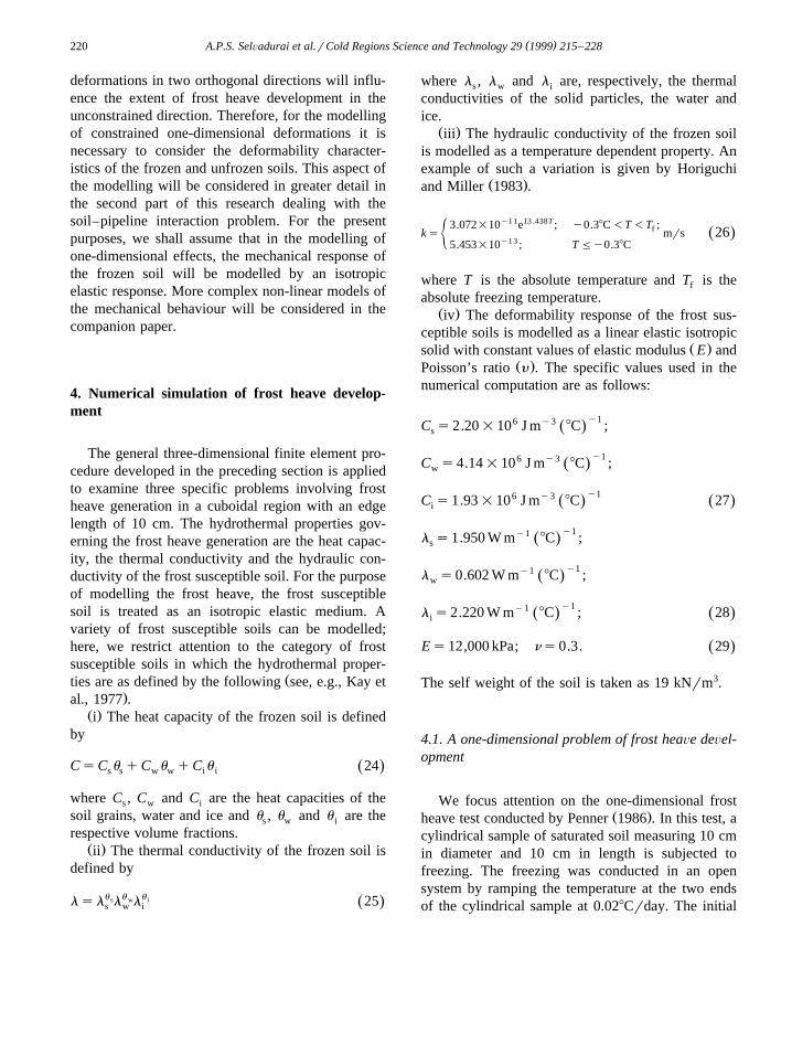
Ž .iii The hydraulic conductivity of the frozen soilis modelled as a temperature dependent property. Anexample of such a variation is given by Horiguchi

Ž .and Miller 1983 .

3.072=10y11e13 .438T ; y0.38C -T -T ;fks mrs 26Ž .½ y1 35.453=10 ; T Fy0.38C

where T is the absolute temperature and T is thef

absolute freezing temperature.Ž .iv The deformability response of the frost sus-

ceptible soils is modelled as a linear elastic isotropicŽ .solid with constant values of elastic modulus E and

Ž .Poisson’s ratio y . The specific values used in thenumerical computation are as follows:

y16 y3C s2.20=10 J m 8C ;Ž .s

y16 y3C s4.14=10 J m 8C ;Ž .w

y16 y3C s1.93=10 J m 8C 27Ž . Ž .i

y1y1l s1.950 W m 8C ;Ž .s

y1y1l s0.602 W m 8C ;Ž .w

y1y1l s2.220 W m 8C ; 28Ž . Ž .i

Es12,000 kPa; ns0.3. 29Ž .

The self weight of the soil is taken as 19 kNrm3.

4.1. A one-dimensional problem of frost heaÕe deÕel-opment

We focus attention on the one-dimensional frostŽ .heave test conducted by Penner 1986 . In this test, a

cylindrical sample of saturated soil measuring 10 cmin diameter and 10 cm in length is subjected tofreezing. The freezing was conducted in an opensystem by ramping the temperature at the two endsof the cylindrical sample at 0.028Crday. The initial


temperature at the top of the sample was 0.558C andthe temperature at the base of the sample was speci-fied at y0.358C. The resulting time-dependent frostheave and the frost penetration were recorded. Thefinite element procedure was used to examine thisone-dimensional problem. Fig. 1 shows the three-di-mensional finite element configuration used to modelthe one-dimensional frost heave problem. Although

the configuration of the finite element discretizationis three-dimensional, the boundary conditions appli-cable to heat conduction, moisture transport anddeformations are organized in such a way that thehydro-thermo-mechanical processes result in a one-dimensional problem. The analysis is therefore appli-cable to the one-dimensional experimental configura-

Ž .tion discussed by Penner 1986 .

Fig. 1. Finite element discretization of the cuboidal element.


Fig. 2. Frost heave generation in a sample of silty clay.

Ž .The paper by Penner 1986 records the develop-ment of frost heave in an experiment which lasted

approximately 250 h. Unfortunately, there is norecord of the hydro-thermo-mechanical parameters

Fig. 3. Influence of hydraulic conductivity on the generation of frost heave.


Fig. 4. Influence of hydraulic conductivity on the generation of frost heave.

applicable to the particular soil. The thermal conduc-tivity and heat capacity parameters used in the com-putational modelling correspond to the generalized

Ž . Ž .results given by Eqs. 24 and 25 and the associ-Ž . Ž .ated constants defined by Eqs. 27 and 28 . The

hydraulic conductivity data are represented by the

Fig. 5. One-dimensional frost heave generation in a sample of Caen silt.


Ž Ž ..result Eq. 26 . Since the hydraulic conductivity ofthe frost susceptible soil is an important parameter inthe problem, its value is varied according to

3.072C=10y11e13 .438T ; y0.38C -T -T ;fks mrs 30Ž .½ y1 35.453C=10 ; T Fy0.38C

Ž .where Cg 1,10 .Fig. 2 shows the comparison of the results of the

finite element techniques proposed in this study withŽ .the experimental results obtained by Penner 1986 .

These calibration results have been obtained by vary-ing the value of the hydraulic conductivity and thespecific value used in the computations correspond-ing to the case where Cs9.5. Fig. 3 illustrates theinfluence of k on the magnitude of frost heave. As isevident, the reduction in the hydraulic conductivityresults in an attendant reduction in the magnitude ofthe frost heave.

Computations were also performed by assigningthe hydraulic conductivity values that are applicableto Caen silt. This silty clay material was used in theexperiments conducted to determine the influence of

discontinuous frost heave developments on the be-Žhaviour of a buried pipeline Dallimore and Williams,

.1984 . Estimates for the hydraulic conductivity ap-plicable to Caen silt given by Shen and LadanyiŽ .1991 are as follows;

1.075=10y9 e23 .99T ; y0.38C -T -T ;fks mrs 31Ž .½ y1 38.0499=10 ; T Fy0.38C

Fig. 4 illustrates the time-dependent evolution ofone-dimensional frost heave in a cuboidal elementwith edge length of 10 cm. The results obtained by

Ž .Shen and Ladanyi 1987 for the specific case whenŽ .the permeability is defined by Eq. 31 and the

Ž .experimental results obtained by Penner 1986 arealso shown for purposes of comparison. The resultsgiven in Fig. 4 indicate that the development of frostheave under one-dimensional conditions obtained bythe computational modelling can be matched reason-ably well with observations of one-dimensional ex-periments. In particular, the trends of the computa-tional results agree very closely with experimentalresults.

Fig. 6. Temperature contours within a cuboidal of Caen silt.


Extensive experiments were conducted by Dal-Ž .limore 1985 to determine the frost heave character-

istics of Caen silt. The results given by DallimoreŽ .1985 are for short-term durations and the condi-tions of the testing which lead to wide variations inthe measured heave are not discussed in detail. Theselection of an extensive set of results for the pur-poses of comparison with the computational predic-tions cannot, therefore, be achieved with confidence.In this study, some typical experimental results have

been selected to cover a 100 h period. Also, thehydraulic conductivity has been modified to the form

16.255=10y9 e23 .99T ; y0.38C -T -T ;fks mrs 32Ž .½ y1 212.07=10 ; T Fy0.38C

Fig. 5 shows the set of experimentally derivedfrost heave data from the tests on Caen silt obtained

Ž .by Dallimore 1985 . It also illustrates the results ofthe corresponding numerical simulation. It is evidentthat the trends in a particular experiment can be

Fig. 7. Surface heave of a cuboidal element subjected to base freezing along a line of edge nodes.


modelled reasonably well by the computationalmodel. The absence of continuous monitoring of thefrost heave generation in the experiment makes itdifficult to establish complete confidence in the cor-relation between the experimental result and thecomputational estimates particularly in the initialstages of the experiment.

4.2. A two-dimensional problem of frost heaÕe deÕel-opment

The computational modelling procedure was usedto examine the two dimensional problem of frostheave development in a cuboidal element with anedge length of 10 cm. The two-dimensional process

of the frost heave development is achieved by allow-ing the freezing action to develop along a line ofelements located at the edge of the cuboidal element.For the purposes of the computational modelling, thethermal and mechanical properties of the soil areidentical to those used in the one-dimensional mod-elling and the hydraulic conductivity values are de-

Ž Ž ..fined by those applicable to Caen silt Eq. 31 . Thesurface temperature of the cuboidal element is main-tained at 0.558C. Fig. 6 illustrates the temperature

Ž .contours within one plane xs0 of the cuboidalelement for lapsed times of ts100 and 233 h. It isevident that the pattern of heat conduction is consis-tent with the imposed thermal boundary conditions.

Fig. 8. Surface heave of a cuboidal element subjected to base freezing at two edge nodes.


We now focus on the development of frost heaveat the surface of the element due to the internalcooling along a line of nodes located along the baseof the element. Fig. 7 illustrates the development offrost heave at the surface of the cuboidal element forelapsed times of 50 and 233 h. Again, the frost heaveprofiles are consistent with the boundary conditionsassociated with the cuboidal element. The surfaceheave profile above the line of nodes subjected tofreezing has a zero slope. This is a requirement ofsymmetry.

4.3. A three-dimensional problem of frost heaÕedeÕelopment

We now consider the three-dimensional problemwhere the cuboidal element is subjected to cooling atthe base of the element at two node locations. Thehydrothermal parameters and the mechanical param-eters used in the computations are identical to thoseused in the one- and two-dimensional problems de-scribed previously. Fig. 8 illustrates the developmentof frost heave at the surface of the cuboidal elementfor elapsed times of 50 and 233 h. Again, it isevident that the frost heave patterns are consistentwith the cooling of isolated nodes located at the baseof the cuboidal element.

5. Concluding remarks

An objective of this study is to develop a plausi-ble frost heave model which can be used to examinethe problem of frost heave induced soil–pipelineinteraction at a discontinuous frost heave zone. Therequirements of such a model are that it should takeinto account the basic coupled processes of heatconduction and moisture transport within an evolv-ing frost heave zone and be capable of demonstratingtrends in frost heave generation consistent with ex-perimental data. Also, the thermo-physical parame-ters required to conduct computational modellingshould be obtainable from either laboratory testsandror in situ tests. The heat conduction and hydro-dynamic coupled model of frost action in soils pre-

Ž .sented by Shen and Ladanyi 1987 is proposed as amodel which could be utilized for frost heave mod-elling. A generalized computational procedure which

incorporates this model is used to develop numericalsolutions to one-, two- and three-dimensional prob-lems of frost heave generation. Comparisons withresults of one-dimensional experiments of frost heavedevelopment indicates that the computational proce-dure can adequately duplicate the trends observed inthe experiments. The results of two- and three-di-mensional problems indicate heat conduction andsurface heave patterns which could be expected inexperimental situations. The parametric studies con-ducted using this coupled model indicates that thehydraulic conductiÕity of the soil is a key parameterwhich governs the rate of fluid influx and conse-quently the magnitude of the frost heave. The accu-rate determination of the hydraulic conductivity ofthe frost susceptible soil is regarded as an essentialprerequisite for the accurate estimation of frost heave.

References

Ž .Andersland, O.B., Anderson, D.M. Eds. , 1978. GeotechnicalEngineering for Cold Regions. McGraw-Hill, New York.

Andersland, O.B., Ladanyi, B., 1994. An Introduction to FrozenGround Engineering. Chapman & Hall, New York.

Anderson, D.M., Williams, P.J., Guymon, G.L., Kane, D.L.,1984. Principles of Soil Freezing and Frost Heaving, Tech.Council on Cold Regions Engineering Monography, FrostAction and Its Control. ASCE, New York, NY, pp. 1–21.

Bathe, K.-J., 1982. Finite Element Procedures in EngineeringAnalysis. Prentice-Hall, Englewood Cliffs, NJ.

Blanchard, D., Fremond, M., 1985. Soils, frost heaving and thawŽ .settlement. In: Kinosita, S., Fukuda, M. Eds. , Ground Freez-

ing, Proc. 4th Int. Symp. on Ground Freezing. A.A. Balkema,Rotterdam, The Netherlands, pp. 209–216.

Dallimore, S.R., 1985. Observations and Predictions of FrostHeave Around a Chilled Pipeline, MA Thesis, Carleton Uni-versity.

Dallimore, S.R., Williams, P.J., 1984. Pipelines and Frost Heave:A Seminar. Carleton University, Ottawa, 75 pp.

Fremond, M., Mikkola, M., 1991. Thermomechanical modellingof freezing soil. Ground Freezing ’91, pp. 17–24.

Hartikainen, J., Mikkola, M., 1997. General thermomechanicalmodel of freezing soil with numerical application. In:

Ž .Knutsson, S. Ed. , Ground Freezing ’97, Proceedings of theInternational Symposium on Ground Freezing and Frost Ac-tion in Soils, Lulea, Sweden. A.A. Balkema, The Netherlands,pp. 101–105.

Holden, J.T., Piper, D., Jones, R.H., 1985. Some observations ofthe rigid-ice model of frost heave. In: Kinosita, S., Fukuda, M.Ž .Eds. , Ground Freezing, Proc. 4th Int. Symp. on GroundFreezing. A.A. Balkema, Rotterdam, The Netherlands, pp.93–98.


Horiguchi, K., Miller, R.D., 1983. Hydraulic conductivity func-tions of frozen materials. Proc. 4th Int. Conf. on Permafrost,pp. 504–508.

Ž .Jessburger, H.L. Ed. , 1979. Ground Freezing, Developments inGeotechnical Engineering, Vol. 26. Elsevier, Amsterdam, TheNetherlands.

Ž .Jones, R.H., Holden, J.T. Eds. , 1988. Ground Freezing ’88,Proc. 5th Int. Symposium on Ground Freezing, Nottingham,UK. A.A. Balkema, Rotterdam, The Netherlands.

Kay, B.D., Perfect, E., 1988. State of the art: heat and massŽ .transfer in freezing soils. In: Jones, R.H., Holden, J.T. Eds. ,

Proc. 5th Int. Symp. on Ground Freezing, Nottingham, UK.A.A. Balkema, Rotterdam, The Netherlands, pp. 3–21.

Kay, B.D., Sheppard, M.I., Loch, J.P.G., 1977. A preliminarycomparison of simulated and observed water redistribution insoils freezing under laboratory and field conditions. Proc. Int.Symp. Frost Action in Soils, Vol. 1, Lulea, pp. 42–53.

Ž .Kinosita, S., Fukuda, M. Eds. , 1985. Ground Freezing ’85, Proc.4th Int. Symp. of Ground Freezing, Sapporo, Japan. A.A.Balkema, Rotterdam, The Netherlands.

Ž .Knutsson, S. Ed. , 1997. Ground Freezing ’97. Proc. 8th Int.Symp. on Ground Freezing, Lulea, Sweden. A.A. Balkema,Rotterdam, The Netherlands.

Konrad, J.M., 1984. ASME Winter Annual Meeting, New Or-leans, Heat Transfer Division, ASME Paper 84-WArHT-108,7 pp.

Konrad, J.M., 1987. Procedure for determining the segregationpotential of freezing soils. Geotechnical Testing Journal,ASTM 10, 51–58.

Konrad, J.M., Duquennois, C., 1993. A model for water transportand ice lensing in freezing soil. Water Resources Research 29,3109–3124.

Konrad, J.M., Morgenstern, M., 1984. Frost heave prediction ofchilled pipelines buried in unfrozen soil. Canadian Geotechni-cal Journal 21, 100–115.

Kujala, K., 1997. Estimation of frost heave and thaw weakeningby statistical analyses and physical models. In: Knutsson, S.Ž .Ed. , Ground Freezing ’97, Proceedings of the InternationalSymposium on Ground Freezing and Frost Action in Soils,Lulea, Sweden. A.A. Balkema, The Netherlands, pp. 31–42.

Lewis, R.W., Schrefler, B.A., 1987. The Finite Element Methodin the Deformation and Consolidation of Porous Media. Wi-ley, New York.

Lewis, R.W., Sze, W.K., 1988. A finite element simulation of

Ž .frost heave in soils. In: Jones, R.H., Holden, J.T. Eds. , Proc.5th Int. Symp. on Ground Freezing, Nottingham, UK. A.A.Balkema, Rotterdam, The Netherlands, pp. 73–80.

Morgenstern, N., 1981. Geotechnical engineering and frontierresource development. Geotechnique 31, 305–365.

National Academy Press, 1984. Ice Segregation and Frost Heav-ing. Washington, DC.

Nixon, J.F., 1987a. Pipeline frost heave prediction using thesegregation potential frost heave method. Proc. Offshore Me-

Ž .chanics and Arctic Engineering OMAE Conf., Houston, TX,pp. 1–6.

Nixon, J.F., 1987b. Thermally induced frost heave beneath chilledpipelines in frozen ground. Canadian Geotechnical Journal 24,260–266.

Penner, E., 1986. Aspects of ice lens growth in soils. ColdRegions Science and Technology 13, 91–100.

Phukan, A., 1985. Frozen Ground Engineering. Prentice-Hall,Englewood Cliffs, NJ.

Ž .Phukan, A. Ed. , 1993. Frost in Geotechnical Engineering. A.A.Balkema, Rotterdam, The Netherlands.

Saarelainen, S., 1992. Modelling of Frost Heaving and FrostPenetration in Soils at Some Observations Sites in Finland,The SSR Model, Tech. Research Centre of Finland, Publica-tion 95, Espoo, Finland.

Selvadurai, A.P.S., 1996. Heat-induced moisture movement in aclay barrier: II. Computational modelling and comparison withexperimental results. Engineering Geology 41, 219–238.

Selvadurai, A.P.S., Nguyen, T.S., 1995. Computational modellingof isothermal consolidation of fractured porous media. Com-puters and Geotechnics 17, 39–73.

Shen, M., Ladanyi, B., 1987. Modelling of coupled heat, moistureand stress field in freezing soil. Cold Regions Science andTechnology 14, 237–246.

Shen, M., Ladanyi, B., 1991. Soil–pipeline interaction duringfrost heave around a buried chilled pipeline. In: Sodhi, D.S.Ž .Ed. , Cold Regions Engineering, ASCE 6th Int. SpecialtyConf. ASCE Publications, New York, NY, pp. 11–21.

Talamucci, F., 1997. Some recent mathematical results on theŽ .problem of soil freezing. In: Knutsson, S. Ed. , Ground

Freezing ’97, Proceedings of the International Symposium onGround Freezing and Frost Action in Soils, Lulea, Sweden.A.A. Balkema, The Netherlands, pp. 179–186.

Zienkiewicz, O.C., Taylor, R.L., 1989. The Finite ElementMethod. McGraw-Hill, New York, NY.

computational modelling of frost heave induced … · cold regions science and technology 29 1999...

Documents