Physics Letters A 367 (2007) 423–430

www.elsevier.com/locate/pla

Constraining a double component dark energy modelusing supernova type Ia data

J.C. Fabris a,∗, S.V.B. Gonçalves a, Fabrício Casarejos b, Jaime F. Villas da Rocha b

a Departamento de Física, Universidade Federal do Espírito Santo, 29060-900 Vitória, Espírito Santo, Brazilb Instituto de Física, Universidade Estadual do Rio de Janeiro, 20550-900 Rio de Janeiro, Brazil

Received 20 October 2006; received in revised form 21 February 2007; accepted 12 March 2007

Available online 16 May 2007

Communicated by P.R. Holland

Abstract

A two-component fluid representing dark energy is studied. One of the components has a polytropic form, while the other has a barotropicform. Exact solutions are obtained and the cosmological parameters are constrained using supernova type Ia data. In general, an open universe ispredicted. A big rip scenario is largely preferred, but the dispersion in the parameter space is very high. Hence, even if scenarios without futuresingularities cannot be excluded with the allowed range of parameters, a phantom cosmology, with an open spatial section, is a general predictionof the model. For a wide range of the equation of state parameters there is an asymptotic de Sitter phase.© 2007 Elsevier B.V. All rights reserved.

PACS: 98.80.-k; 98.80.Es

1. Introduction

Several cosmological observables indicate that the presentUniverse is in a state of accelerated expansion. The first evi-dence in this sense came in the end of the last decade, whentwo independent observational projects [1], using type Ia su-pernovae luminosity distance-redshift relation, provided an es-timation of the deceleration parameter q = −aa/a2. With acatalogue of about 50 type Ia supernova with low and highredshifts, the analysis revealed a negative q , indicating an ac-celerated Universe. Today, more than 300 type Ia supernovaehave been identified, with high redshift, and the conclusion thatq is negative remains [2]. Since then, there has been an exten-sive discussion on the quality of the data. This led to a restrictedsample of 157 supernova, called the “gold sample” [3]. A morerecent survey led to the so-called “legacy sample”, of about 100supernova, with high quality data [4]. Even if the precise esti-

* Corresponding author.E-mail addresses: fabris@cce.ufes.br (J.C. Fabris), sergio@cce.ufes.br

(S.V.B. Gonçalves), fabll@dft.if.uerj.br (F. Casarejos), roch@dft.if.uerj.br(J.F. Villas da Rocha).

0375-9601/$ – see front matter © 2007 Elsevier B.V. All rights reserved.doi:10.1016/j.physleta.2007.03.094

mation of the cosmological parameters, like the matter density,Hubble parameter, etc., depends quite strongly on the choice ofthe sample, the conclusion that the Universe is accelerating hasremained. Hence, a large part of the community of cosmologistaccepts the present acceleration of the Universe as a fact.

A combination data from CMB anisotropies of the cosmicmicrowave background radiation [5], large scale structure [6]and type Ia supernovae data [7], indicates an almost flat Uni-verse, ΩT ∼ 1 and a matter (zero effective pressure) density pa-rameter of order Ωm ∼ 0.3 [8]. Since an accelerated expansioncan be driven by a repulsive effect, which can be provided by anexotic fluid with negative pressure, it has been concluded thatthe Universe is also filled by an exotic component, called darkenergy, with density parameter Ωc ∼ 0.7. This exotic fluid leadsto an accelerated expansion, remaining at same time smoothlydistributed, not appearing in the local matter clustering.

The first natural candidate to represent dark energy is a cos-mological constant, which faces, however, many well-knownproblems. More recently, other candidates have been studied inthe literature: quintessence, k-essence, Chaplygin gas, amongmany others. For a review of these proposals, see reference [9].There are also claims that a phantom field (fields with a large

424 J.C. Fabris et al. / Physics Letters A 367 (2007) 423–430

negative pressure such that all energy conditions are violated)leads to the best fit of the observational data [10]. A phantomfield implies a singularity in a finite future proper time, whichhas been named big rip, where density and curvature diverge.This is of course an undesirable feature, but more detailed the-oretical and observational analyses must be made in order toverify this scenario. Some authors state, based on considera-tions about the evaluation of the cosmological parameters, thatthere is no such phantom menace [11]. This is still an object ofdebate.

Most of the studies made until now lay on the assumptionof a simple relation between pressure and density expressedgenerically, in a hydrodynamical representation, by p = wρα .Quintessence, like others dark energy candidates, imply that w

varies with the redshift, not being a constant. Chaplygin gasmodels (generalized or not) [12] imply a general value for α,but typically negative, and w < 0. Phantom fields could be rep-resented by α = 1, w < −1. Due to the high speculative natureof the dark energy component, many possibilities have beenconsidered in the literature, both from fundamental or phenom-enological point of views.

In the present work we intend to exploit a more generic re-lation between pressure and density with respect to those casesnormally considered. The main idea is to use a double com-ponent equation of state. The relation between pressure anddensity may be written as

(1)pe = −k1ραc − k2ρc,

where α, k1 and k2 are constants, and the subscript c indicatesthat such relation concerns the dark energy component of thematter content of the Universe. Let us call the component la-belled by k1 as the polytropic component, and that one labelledby k2 as the barotropic component. This kind of equation ofstate has been, for example, studied in a theoretical sense inreference [13].

The equation of state (1) may be also seen as a realisationof the so-called modified Chaplygin gas [14–16]. The usualChaplygin gas model, generalised or not, has been introduced inorder to obtain an interpolation between a matter dominated eraand a de Sitter phase [12]. The modified Chaplygin gas modelallows to obtain an interpolation between, for example, a radia-tive era and a �CDM era. In general, in this case, a negativevalue for α is considered. But, as it will be seen later, even for apositive value of α, such an interpolation is possible. From thefundamental point of view, the equation of state (1) can be ob-tained in terms of self-interacting scalar field. In Refs. [14–16]a connection with the rolling tachyon model has been estab-lished. This allows to consider the equation of state (1) as aphenomenological realisation of a string specific configuration.

In Ref. [17], a structure similar to (1) has been analysed,using observational data, but fixing k2 = 1, with the conclu-sion that the fitting of the supernova data are quite insensitiveto the parameter α. Here, we follow another approach: we willfix α = 1/2, leaving k2 free. This has the advantage of leadingto explicit analytical expressions for the evolution of the Uni-verse. Moreover, and perhaps more important, this may lead tointeresting scenarios where, for example, the Universe evolves

asymptotically as in a de Sitter phase, even if the equation ofstate is not characteristic of the vacuum state, p = −ρ.

We will test the equation of state (1) against type Ia super-novae data. We will span a four-dimensional phase space, usingas free parameters the dark matter density parameter Ωm0, theexotic fluid density parameter Ωc0 (or alternatively, the curva-ture parameter Ωk0), the Hubble parameter H0, and the equa-tion of state parameter k1 or k2. The subscript 0 indicates thatall these quantities are evaluated today. Using the gold sample,we will show that the preferred values indicate k2 ∼ 6, Ωm0 andΩc0 ∼ 0.3, and H0 ∼ 67. An open universe is a general predic-tion for this model. A phantom behaviour is largelly favoured.However, the dispersion is very high, and an asymptotic cos-mological constant phase cannot be discarded.

The use of other observables, like the spectrum of theanisotropy of the cosmic microwave background radiation(CMB) and the matter power spectrum, can in principle restrictmore severely the parameter space. However, we postpone thisevaluation to a future study because, in both cases, a perturba-tive analysis of the model is necessary. In this case we mustreplace the hydrodynamical representation presented above bya fundamental description of the fluid, for example, in termsof self-interacting scalar fields. We note en passant that thehydrodynamical representation employed here may lead, at per-turbative level, to instabilities at small scales due to a imaginaryeffective sound velocity, instabilities that can be avoided witha fundamental representation [18]. There are many differentways to implement this more fundamental description, whichcan lead to different results. The supernova data, on the otherhand, test essentially the background, which is somehow inde-pendent of the description of the fluid.

The Letter is organised as follows. In the next section, weobtain some analytical expressions for the evolution of the Uni-verse, and derive the luminosity distance relation for the model.In Section 3, we make the comparison between the theoreticalmodel and the observational data. In Section 4, we present ourconclusions.

2. The evolution of the Universe

Let us consider the equations of motion when the exotic fluidgiven by the equation of state (1) dominates the matter contentof the Universe. The Friedmann’s equation and the conservationof the energy-momentum tensor read,

(2)

(a

a

)2

+ k

a2= 8πG

3ρc,

(3)ρc + 3a

a(ρc + pc) = 0,

where k is the curvature of the spatial section. Inserting Eq. (1),with α = 1/2, in Eq. (3), it comes out that the exotic fluid den-sity depends on the scale factor as

(4)ρc = 1

β2

[k1 + v0a

− 32 β

]2,

J.C. Fabris et al. / Physics Letters A 367 (2007) 423–430 425

where β = 1−k2. Introducing this result in Eq. (2), it is possibleto obtain an explicit solution for the scale factor when k = 0:

(5)a = a0{exp[k1M t] − c0

} 23β ,

where a0 and c0 are integration constants. The constants obeythe relations

(6)M = √6πG, c0 = v0

k1a

− 32 β

0 .

This solution can always represent an expanding Universe, withan initial singularity. Moreover, when k2 > 1, the density goesto infinity as the scale factor goes to infinity, in a finite propertime, characterising a big rip. However, if k2 < 1, the expansionlasts forever, and becomes asymptotically de Sitter even if k2 �=1 (the strict cosmological constant case). Initially, the scale fac-tor behaves as in the pure barotropic case with p = −k2ρ.

The particular case where k2 = 1, but with free α, has beenanalysed in Ref. [17]. For our case, fixing α = 1/2 and k2 = 1,the relation between density and scale factor becomes,

(7)ρc =(

3

2k1 − 1

)lna.

If we consider the dynamics of a universe driven by theexotic fluid defined by Eq. (1) and pressureless matter, the equa-tions of motion are given by,

(8)H 2 =(

a

a

)2

= 8πG

3(ρm + ρc) − k

a2,

(9)ρm + 3a

aρm = 0,

(10)ρc + 3a

a(ρc + pc) = 0,

where pc is given by Eq. (1). The conservation Eqs. (9), (10)can be integrated, again for α = 1/2, leading to the relation (4)and ρm = ρm0/a

3. In this case, it does not seem possible toobtain a closed expression for the scale factor in terms of thecosmic time t as before. However, the inclusion of the pres-sureless component is essential in order to take into account theeffects of the baryons in the determination of the allowed rangefor the parameters of the model using the supernova data, as itwill be done in the next section.

3. Fitting type Ia supernovae data

As time goes on, more and more high redshift type Ia super-novae are detected. Today, about 300 high z SN Ia have beenreported. However, there are many discussions on the quality ofthese data. A “gold sample”, with the better SN Ia data, with anumber of 157 SN, has been proposed [3]. More recently, theSupernova Legacy Survey (SNLS) was made public, containingaround 100 SNIa [4]. In this work, we will use the gold sample.This will allows us to compare our results with previous onesusing a similar method, but with different models [7].

From now on, we will normalise the scale factor, makingit equal to one today: a0 = 1. Hence, the relation between thescale factor a and the redshift z becomes 1 + z = 1/a. In order

to compare the observational data with the theoretical values,the fundamental quantity is the luminosity distance [19,20],given by

(11)DL = (1 + z)r,

where r is the comoving radial position of the supernova. For aflat Universe, the comoving radial coordinate is given by

(12)r =z∫

0

dz′

H(z′).

Using Eq. (8), with the expressions for the exotic and pres-sureless fluid in terms of a, converted to relations for thosecomponents in terms of the redshift z, we obtain the depen-dence of the Hubble parameter in terms of z. Hence, the finalexpression for the luminosity distance is, for our model withk2 �= 1,

DL = c(1 + z)

H0

z∫0

{Ωm0(1 + z′)3 + Ωk0(1 + z′)2

+ Ωc0

[(1 − k1

1 − k2

)(1 + z′)3

(1−k2)

2

(13)+ k1

1 − k2

]2}−1/2

dz′.

For the case k2 = 1, the luminosity distance is given by

DL = c(1 + z)

H0

(14)

×z∫

0

dz′√Ωm0(1 + z′)3 + Ωk0(1 + z′)2 + Ωc0{1 − 3

2 k1 ln(1 + z′)}2.

In the expressions above, H0 is the Hubble parameter today,which can be parametrised by h, such that H0 =100 h km/s Mpc. The parameter k1 has been redefined ask1/

√ρc0 → k1, ρc0 being the exotic component density to-

day. This redefinition is made in order to obtain a dimension-less parameter k1. Moreover, Ωm0 = 8πGρm0/(3H 2

0 ), Ωc0 =8πGρc0/(3H 2

0 ) and Ωk0 = −k/H 20 .

The comparison with the observational data is made by com-puting the distance modulus, defined as

(15)μ0 = 5 log

(DL

Mpc

)+ 25,

which is directly connected with the difference between the ap-parent and absolute magnitudes of the supernovae. The qualityof the fitting is given by

(16)χ2 =∑

i

(μo0i − μt

0i )2

σ 20i

,

where μo0i and μt

0i are the observed and calculated distancemoduli for the ith supernova, respectively, while σ 2

0i is the errorin the observational data, taking already into account the effectof the dispersion due to the peculiar velocity.

426 J.C. Fabris et al. / Physics Letters A 367 (2007) 423–430

In principle, the model contains five free parameters: k1, k2,H0, Ωc0 and Ωm0. We will work in a four-dimensional phasespace: for each value of k1, we will vary the other four parame-ters. Thus, the χ2 function will depend on four parameters, Ωc0,Ωm0, H0 and k2. The probability distribution is then given by

(17)P(Ωc0,Ωm0,H0, k2) = Ae− χ2(Ωc0,Ωm0,H0,k2)

2σ ,

where A is a normalisation constant and σ is directly related tothe confidence region. The graphics and the parameter estima-tions were made using the software BETOCS [21].

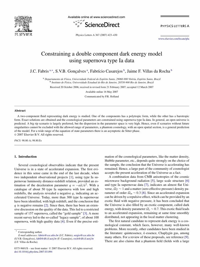
The multidimensional plot of the probability distribution isnot, in general, the best way to have an overview of the results.However, we can construct a two-dimensional probability dis-tribution, integrating in two of the parameters. In Fig. 1, wedisplay the Probability Density Function, PDF, after integrat-ing the distribution (17) in the variables H0 and k2: a two-dimensional probability distribution is obtained for the vari-ables Ωm0 and Ωc0, and with k1 = 0 and 1.0. The plots show theconfidence regions at 1σ (68%), 2σ (95%) and 3σ (99%) levels.This two-dimensional probability distribution reveals that thematter density parameters have their higher probability aroundΩm0,Ωc0 ∼ 0.3. An open model is clearly preferred. This isalso evident in Fig. 2, where the two-dimensional probabilitydistribution for Ωk0 and Ωm0 is shown. Such preference foran open model contrast strongly with a similar analysis for the�CDM and Chaplygin gas models, for which a closed universeis clearly preferred [7]. As the value of k1 grows, a low densityuniverse becomes more favoured, as it can be seen in Table 1.In this table, we include also the case k1 = 0.5 to show moreexplicitely that the parameter estimations change very slightlywith k1.

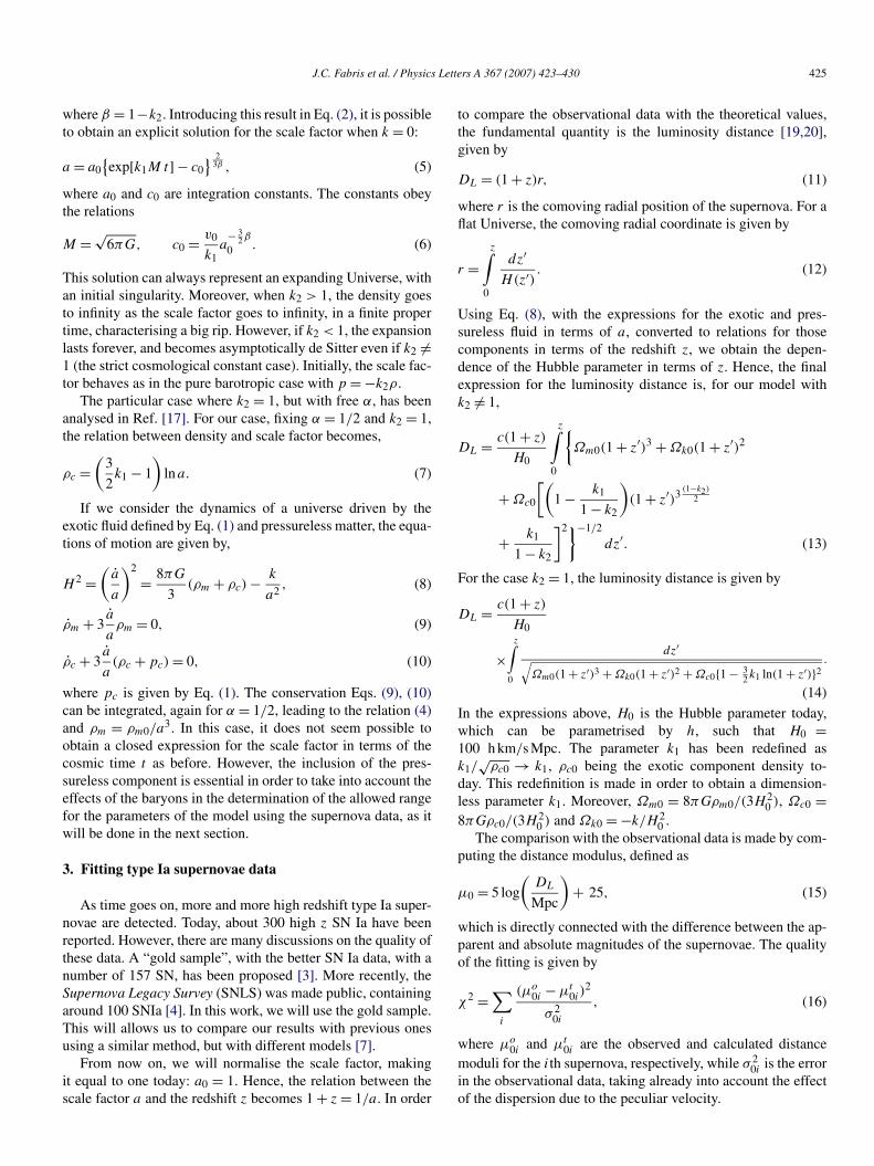
In Fig. 3, the two-dimensional PDF is displayed when weintegrate on Ωm0 and H0, remaining with k2 and Ωc0. As in

the preceding case, a low density parameter for the dark energycomponent is preferred. What is specially interesting is thatthe values of k2 larger than 1 and until around 40 have higherprobabilities. This means that a phantom scenario is clearlyfavoured. The peak of probability for k2 occurs near 5–6. Asthe value of k1 increases, the peak probability for k2 occurs at alower value.

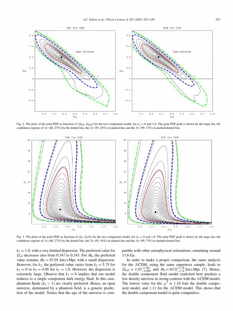
In Fig. 4, the two-dimensional PDF is displayed when we in-tegrate on Ωm0 and Ωc0, obtaining a two-dimensional graphicfor k2 and H0. It is interesting to note, now, that regions aroundH0 ∼ 70 km Mpc s are preferred. This may reconcile the estima-tions obtained using supernova with those obtained using CMBand matter clustering, which indicates H0 around 72 km Mpc s[6,22]. The preferred value for H0 depends very little on k1.

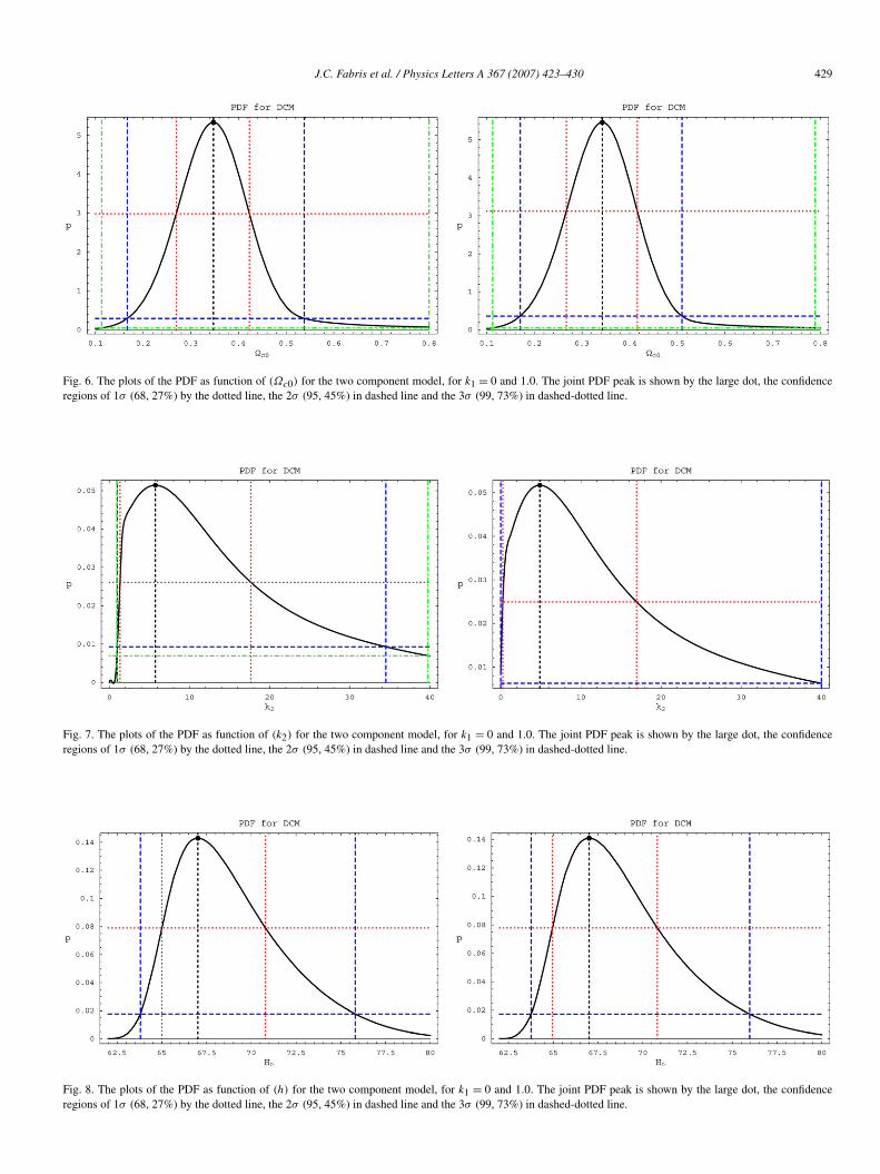
A more precise estimation of the parameters can be obtainedby evaluating the one-dimensional PDF, by integrating on thethree other parameters. The results are displayed in Figs. 5–8,and confirm what has been said based on the two-dimensionalgraphics. The error bars at 1σ , 2σ and 3σ confidence levelsare indicated. For the matter density parameter, its preferredvalue varies from Ωm0 = 0.233 for k1 = 0 to Ωm0 = 0.228, for

Table 1Estimated values for Ωm0, Ωc0, Ωk0, H0, k2 and t0 for three different valuesof k1, at 2σ level

k1 0.0 0.5 1.0

Ωm0 0.233+0.303−0.171 0.231+0.305

−0.172 0.228+0.0.304−0.172

Ωc0 0.347+0.191−0.181 0.345+0.180

−0.178 0.343+0.167−0.172

Ωk0 0.408+0.317−0.467 0.412+0.317

−0.457 0.415+0.318−0.439

H0 67.01+8.80−3.21 67.01+8.89

−3.24 67.01+8.97−3.24

k2 5.75+28.74−4.75 5.35+28.89

−4.85 4.88+35.12−4.88

t0 13.64+1.20−0.74 13.65+1.20

−0.75 13.65+1.22−.075

Fig. 1. The plots of the joint PDF as function of (Ωc0,Ωm0) for the two component model, for k1 = 0 and 1.0. The joint PDF peak is shown by the large dot, theconfidence regions of 1σ (68, 27%) by the dotted line, the 2σ (95, 45%) in dashed line and the 3σ (99, 73%) in dashed-dotted line.

J.C. Fabris et al. / Physics Letters A 367 (2007) 423–430 427

Fig. 2. The plots of the joint PDF as function of (Ωk0,Ωm0) for the two component model, for k1 = 0 and 1.0. The joint PDF peak is shown by the large dot, theconfidence regions of 1σ (68, 27%) by the dotted line, the 2σ (95, 45%) in dashed line and the 3σ (99, 73%) in dashed-dotted line.

Fig. 3. The plots of the joint PDF as function of (k2,Ωc0) for the two component model, for k1 = 0 and 1.0. The joint PDF peak is shown by the large dot, theconfidence regions of 1σ (68, 27%) by the dotted line, the 2σ (95, 45%) in dashed line and the 3σ (99, 73%) in dashed-dotted line.

k1 = 1.0, with a very limited dispersion. The preferred value forΩc0 decreases also from 0.347 to 0.343. For H0, the preferredvalue remains H0 = 67.01 km/s Mpc with a small dispersion.However, for k2, the preferred value varies from k2 = 5.75 fork1 = 0 to k2 = 4.88 for k1 = 1.0. However, the dispersion isextremely large. Observe that k1 = 0 implies that our modelreduces to a single component dark energy fluid. In this case,phantom fluids (k2 > 1) are clearly preferred. Hence, an openuniverse, dominated by a phantom field, is a generic predic-tion of the model. Notice that the age of the universe is com-

patible with other astrophysical estimations, remaining around13.6 Gy.

In order to make a proper comparison, the same analysisfor the �CDM, using the same supernova sample, leads toΩm0 = 1.01+1.08

−0.085 and H0 = 65.0+1.78−1.74 km s Mpc [7]. Hence,

the double component fluid model exploited here predicts alow density universe in strong contrast with the �CDM model.The lowest value for the χ2 is 1.10 four the double compo-nent model, and 1.11 for the �CDM model. This shows thatthe double component model is quite competitive.

428 J.C. Fabris et al. / Physics Letters A 367 (2007) 423–430

Fig. 4. The plots of the joint PDF as function of (k2,H0) for the two component model, for k1 = 0 and 1.0. The joint PDF peak is shown by the large dot, theconfidence regions of 1σ (68, 27%) by the dotted line, the 2σ (95, 45%) in dashed line and the 3σ (99, 73%) in dashed-dotted line.

Fig. 5. The plots of the PDF as function of Ωm0 for the two component model, for k1 = 0 and 1.0. The joint PDF peak is shown by the large dot, the confidenceregions of 1σ (68, 27%) by the dotted line, the 2σ (95, 45%) in dashed line and the 3σ (99, 73%) in dashed-dotted line.

4. Conclusion

In this work, we have explored the possibility that the darkenergy has an equation of state given by (1). This proposal hasalready been explored in reference [17], but restricting one ofthe components to behave like a cosmological constant: a two-component fluid, which is a “variation” around a cosmologicalconstant, has been analysed. Here, we alleviate this restriction,but introducing another one: the linear component can have anybarotropic index, but the second component must vary as thesquare root of the density. This allows us to obtain an analyticalexpression for the evolution of the Universe, at least for a flatspatial section. This analytic expression reveals that it is pos-sible to have an asymptotically de Sitter phase, for p < 0 andk2 < 1, even if only k2 = 1 represents the cosmological con-

stant. This is an intriguing aspect of the model. For k2 > 1 thereis always a big rip.

The restriction in the polytropic factor α seems not to be sorelevant in view of the results of reference [17]: if the secondcomponent obeys a polytropic power law, there is a strong de-generacy on the polytropic factor, and almost any value of thepower is allowed.

Our results indicate an open universe with a matter densityparameter around Ωm0 ∼ 0.3, with a similar estimation for thedark energy component. The �CDM model favours a closeduniverse. On the other hand, the predicted value for the Hubbleparameter is more consistent with other observational tests, likeCMB, that is, H0 ∼ 67 km s Mpc [23]. For the barotropic indexin the two-component fluid k2, the results indicate that k2 > 1is highly favoured. The dispersion is very high, but tends still

J.C. Fabris et al. / Physics Letters A 367 (2007) 423–430 429

Fig. 6. The plots of the PDF as function of (Ωc0) for the two component model, for k1 = 0 and 1.0. The joint PDF peak is shown by the large dot, the confidenceregions of 1σ (68, 27%) by the dotted line, the 2σ (95, 45%) in dashed line and the 3σ (99, 73%) in dashed-dotted line.

Fig. 7. The plots of the PDF as function of (k2) for the two component model, for k1 = 0 and 1.0. The joint PDF peak is shown by the large dot, the confidenceregions of 1σ (68, 27%) by the dotted line, the 2σ (95, 45%) in dashed line and the 3σ (99, 73%) in dashed-dotted line.

Fig. 8. The plots of the PDF as function of (h) for the two component model, for k1 = 0 and 1.0. The joint PDF peak is shown by the large dot, the confidenceregions of 1σ (68, 27%) by the dotted line, the 2σ (95, 45%) in dashed line and the 3σ (99, 73%) in dashed-dotted line.

430 J.C. Fabris et al. / Physics Letters A 367 (2007) 423–430

to favour a phantom scenario. As the component index k1 in-creases, the preferred value of k2 decreases slightly.

It must be remarked that the model described here exhibits aχ2 slightly smaller than for the �CDM model. This shows thatthe model is quite competitive. In our opinion, even if a phan-tom scenario is clearly preferred, the fact of predicting a lowdensity universe is interesting in its own, mainly when com-pared with the analysis of clustering of matter in the universe.

Acknowledgements

We thank the anonymous referee who has suggested us, be-sides other remarks, to consider the non-flat case, what hasled to new interesting results with respect to the previous ver-sion of the Letter. We thank also CNPq (Brazil) and CAPES(Brazil) for partial financial support. F.C. and J.F.V.R. thankalso FAPERJ (Brazil) for partial financial support. We thankRoberto Colistete Jr. and Martin Makler for their critical re-marks.

References

[1] A.G. Riess, et al., Astron. J. 116 (1998) 1009;S. Perlmutter, et al., Astrophys. J. 517 (1999) 565.

[2] J.L. Tonry, et al., Astrophys. J. 594 (2003) 1.[3] A.G. Riess, Astrophys. J. 607 (2004) 665.[4] P. Astier, et al., Astron. Astrophys. 447 (2006) 31.[5] L. Verde, et al., Astrophys. J. Suppl. 148 (2003) 195.[6] M. Tegmark, et al., Astrophys. J. 606 (2004) 702.

[7] R. Colistete Jr., J.C. Fabris, S.V.B. Gonçalves, P.E. de Souza, Int. J. Mod.Phys. D 13 (2004) 669;R. Colistete Jr., J.C. Fabris, S.V.B. Gonçalves, Int. J. Mod. Phys. D 14(2005) 775;R. Colistete Jr., J.C. Fabris, Class. Quantum Grav. 22 (2005) 2813.

[8] M. Tegmark, et al., Phys. Rev. D 69 (2004) 103501.[9] V. Sahni, Lecture Notes in Physics, vol. 653, Springer, Berlin, 2004, 141.

[10] S. Hannestad, E. Mortsell, JCAP 0409 (2004) 001;U. Alam, V. Sahni, T.D. Saini, A.A. Starobinsky, Mon. Not. R. Astron.Soc. 354 (2004) 275;S.W. Allen, et al., Mon. Not. R. Astron. Soc. 353 (2004) 457.

[11] H.K. Jassal, J.S. Bagla, T. Padmanabhan, astro-ph/0601389.[12] A.Yu. Kamenschik, U. Moschella, V. Pasquier, Phys. Lett. B 511 (2001)

265;J.C. Fabris, S.V.B. Gonçalves, P.E. de Souza, Gen. Relativ Gravit. 34(2002) 53;N. Bilic, G.B. Tupper, R.D. Viollier, Phys. Lett. 535 (2002) 17;M.C. Bento, O. Bertolami, A.A. Sen, Phys. Rev. D 66 (2002) 043507.

[13] S. Mukherjee, B.C. Paul, N.K. Dadhich, S.D. Maharaj, A. Beesham, gr-qc/0605134.

[14] H.B. Benaoum, hep-th/0205140.[15] U. Debnath, A. Banerjee, S. Chakraborty, Class. Quantum Grav. 21 (2004)

5609.[16] W. Chakraborty, U. Debnath, gr-qc/0611094.[17] J.S. Alcaniz, H. Stefancic, astro-ph/0512622.[18] J.C. Fabris, J. Martin, Phys. Rev. D 55 (1997) 5205.[19] S. Weinberg, Gravitation and Cosmology, Wiley, New York, 1972.[20] P. Coles, F. Lucchin, Cosmology, Wiley, New York, 1995.[21] R. Colistete Jr., BayEsian Tools for Observational Cosmology us-

ing SNe Ia (BETOCS), available on the Internet site, http://www.RobertoColistete.net/BETOCS, 2006.

[22] D.N. Spergel, et al., astro-ph/0603449.[23] D.N. Spergel, et al., Astrophys. J. Suppl. 148 (2003) 175.