contemporary electromagnetic spectrum reuse techniques: tv ... · my co-supervisor prof. dr....
TRANSCRIPT
FEDERAL UNIVERSITY OF CEARÁ
DEPARTMENT OF TELEINFORMATICS ENGINEERING
POST-GRADUATE PROGRAM IN TELEINFORMATICS ENGINEERING
CARLOS FILIPE MOREIRA E SILVA
CONTEMPORARY ELECTROMAGNETIC SPECTRUM REUSE TECHNIQUES:TV WHITE SPACES AND D2D COMMUNICATIONS
DOCTOR OF PHILOSOPHY THESIS
SUPERVISOR: PROF. DR. FRANCISCO RODRIGO PORTO CAVALCANTI
CO-SUPERVISOR: PROF. DR. TARCISIO FERREIRA MACIEL
FORTALEZA/CEARÁ
DECEMBER 2015
CARLOS FILIPE MOREIRA E SILVA
TÉCNICAS CONTEMPORÂNEAS DE REUSO DO ESPECTROELECTROMAGNÉTICO: TVWHITE SPACES E COMUNICAÇÕES D2D
Tese apresentada à Coordenação do Programade Pós-Graduação em Engenharia de Teleinfor-mática da Universidade Federal do Ceará comorequisito parcial para a obtenção do título deDoutor em Engenharia de Teleinformática.
Área de Concentração: Sinais e Sistemas.
ORIENTADOR: PROF. DR. FRANCISCO RODRIGO PORTO CAVALCANTI
CO-ORIENTADOR: PROF. DR. TARCISIO FERREIRA MACIEL
UNIVERSIDADE FEDERAL DO CEARÁ
DEPARTAMENTO DE ENGENHARIA DE TELEINFORMÁTICA
PROGRAMA DE PÓS-GRADUAÇÃO EM ENGENHARIA DE TELEINFORMÁTICA
FORTALEZA/CEARÁ
DEZEMBRO 2015
Dados Internacionais de Catalogação na PublicaçãoUniversidade Federal do Ceará
Biblioteca de Pós-Graduação em Engenharia - BPGE
S579c Silva, Carlos Filipe Moreira e.Contemporary electromagnetic spectrum reuse techniques: tv white spaces and D2D
communications / Carlos Filipe Moreira e Silva. – 2015.146 f. : il. color. , enc. ; 30 cm.
Tese (doutorado) – Universidade Federal do Ceará, Centro de Tecnologia, Departamento de Engenharia de Teleinformática, Programa de Pós-Graduação em Engenharia de Teleinformática, Fortaleza, 2015.
Área de concentração: Sinais e Sistemas.Orientação: Prof. Dr. Francisco Rodrigo Porto Cavalcanti.Coorientação: Prof. Dr. Tarcisio Ferreira Maciel.
1. Teleinformática. 2. Espectro eletromagnético. 3. Análise SWOT. I. Título.
CDD 621.38

To my Family, Friends, Lovers, Professors, and
Unknowns that taught me valuable lessons that
raised me as I am today.
—Carlos Filipe Moreira e Silva

“But the real way to get happiness is by giving
out happiness to other people. Try and leave this
world a little better than you found it and when
your turn come to die, you can die happy in
feeling that at any rate you have not wasted
your time but have done your best.”
—Robert Smith Baden Powell
«Fare una tesi signica divertirsi e la tesi è come
il maiale, non se ne butta via niente.»
—Umberto Eco
Acknowledgments
I am thankful to everyone who directly or indirectly have collaborated and helped me in thework throughout the Doctor of Philosophy (PhD) period that gives the basis for this thesis.
First of all, I must express my gratitude to Prof. Dr. Francisco Rodrigo Porto Cavalcantiwho has accepted to be my supervisor even when I was still in Portugal and did not knowme personally, and also for his support, guidance, trust, and advises during the supervisionof my studies. Without him my travel to Brazil would not be possible. I am also grateful tomy co-supervisor Prof. Dr. Tarcisio Ferreira Maciel for his knowledge, teachings, protablediscussions, and incentive during my participation in the research projects in partnership withEricsson.
For all my co-workers and colleagues in both sides of the Atlantic Ocean from the Universityof Aveiro and Telecommunications Institute (Instituto de Telecomunicações, IT)-Aveiro inPortugal, and from the Federal University of Ceará and Wireless Telecommunications ResearchGroup (Grupo de Pesquisa em Telecomunicações Sem Fio, GTEL) in Brazil, with whom I hadprotable discussions and their advices, suggestions, and, especially, friendship were essentialfor the materialization of the thesis.
Everyone needs a spot, thus I am thankful to IT-Aveiro and more recently to GTEL researchgroups, not only for giving me a spot and infrastructure where I could work, but also forthe welcoming during the studies, scholarship, and travelling nancial support. Likewise toPost-Graduation Program in Teleinformatics Engineering (Programa de Pós-Graduação emEngenharia Teleinformática, PPGETI) for the teaching courses and for the travelling nancialsupport that helped me to attend a conference during the PhD period.
The work that gives the basis for the thesis was assisted by the European Commission,Seventh Framework Programme (FP7), under the project 248560, ICT-COGEU, and by theInnovation Center, Ericsson Telecomunicações S.A., Brazil, under EDB/UFC.33 and EDB/UFC.40technical cooperation contracts. I must also acknowledge the Coordenação de Aperfeiçoamentode Pessoal de Nível Superior (CAPES) for the scholarship.
Last but not least, I grateful for everything to every single member of my family that missedme (and I missed them) during this period, especially my mother, my father, my sister, mybother in law, my nice and nephew. Finally, to all my friends (they know who they are) inPortugal and Brasil that gave part of their time to spend with me, listening and advising, eatingand drinking, playing or just walking around, and with whom I shared valuable moments ofmy life.
As someone said, “What if today, we were just grateful for everything?”
This thesis is for you all, thanks!
vi
Abstract
Over the last years, the wireless broadband access has achieved a tremendous success.With that, the telecommunications industry has faced very important changes in terms
of technology, heterogeneity, kind of applications, and massive usage (virtual data tsunami)derived from the introduction of smartphones and tablets; or even in terms of market structureand its main players/actors. Nonetheless, it is well-known that the electromagnetic spectrum isa scarce resource, being already fully occupied (or at least reserved for certain applications). Tra-ditional spectrum markets (where big monopolies dominate) and static spectrum managementoriginated a paradoxal situation: the spectrum is occupied without actually being used!
In one hand, with the global transition from analog to digital Television (TV), part of thespectrum previously licensed for TV is freed and geographically interleaved, originating theconsequent Television White Spaces (TVWS); on the other hand, the direct communicationsbetween devices, commonly referred as Device-to-Device (D2D) communications, are attractingcrescent attention by the scientic community and industry in order to overcome the scarcityproblem and satisfy the increasing demand for extra capacity. As such, this thesis is divided intwo main parts: (a) Spectrum market for TVWS: where a SWOT analysis for the use of TVWSis performed giving some highlights in the directions/actions that shall be followed so that itsadoption becomes eective; and a tecno-economic evaluation study is done considering as ause-case a typical European city, showing the potential money savings that operators may reachif they adopt by the use of TVWS in a exible market manner; (b) D2D communications: wherea neighbor discovery technique for D2D communications is proposed in the single-cell scenarioand further extended for the multi-cell case; and an interference mitigation algorithm basedon the intelligent selection of Downlink (DL) or Uplink (UL) band for D2D communicationsunderlaying cellular networks.
A summary of the principal conclusions is as follows: (a) The TVWS defenders shallfocus on the promotion of a real-time secondary spectrum market, where through the correctimplementation of policies for protection ratios in the spectrum broker and geo-locationdatabase, incumbents are protected against interference; (b) It became evident that an operatorwould recover its investment around one year earlier if it chooses to deploy the networkfollowing a exible spectrum market approach with an additional TVWS carrier, instead ofthe traditional market; (c) With the proposed neighbor discovery technique the time to detectall neighbors per Mobile Station (MS) is signicantly reduced, letting more time for the actualdata transmission; and the power of MS consumed during the discovery process is also reducedbecause the main processing is done at the Base Station (BS), while the MS needs to ensure thatD2D communication is possible just before the session establishment; (d) Despite being a simpleconcept, band selection improves the gains of cellular communications and limits the gainsof D2D communications, regardless the position within the cell where D2D communicationshappen, providing a trade-o between system performance and interference mitigation.
Keywords: Electromagnetic Spectrum Management, Television, TV, TVWS, White Spaces,SWOT Analysis, Tecno-Evaluation, Device-to-Device Communications, D2D, Neighbor Dis-covery, Co-Channel Interference, Band Selection.
vii
Resumo
N os últimos anos, o acesso de banda larga atingiu um grande sucesso. Com isso, a indústriadas telecomunicações passou por importantes transformações em termos de tecnologia,
heterogeneidade, tipo de aplicações e uso massivo (tsunami virtual de dados) em consequênciada introdução dos smartphones e tablets; ou até mesmo na estrutura de mercado e os seusprincipais jogadores/atores. Porém, é sabido que o espectro electromagnético é um recursolimitado, estando já ocupado (ou pelo menos reservado para alguma aplicação). O mercadotradicional de espectro (onde os grandes monopólios dominam) e o seu gerenciamento estáticocontribuíram para essa situação paradoxal: o espectro está ocupado mas não está sendo usado!
Por um lado, com a transição mundial da Televisão (TV) analógica para a digital, parte doespectro anteriormente licenciado para a TV é libertado e geogracamente multiplexado paraevitar a interferência entre sinais de torres vizinhas, dando origem a «espaços em branco» nafrequência da TV ou Television White Spaces (TVWS); por outro lado, as comunicações diretasentre usuários, designadas por comunicações diretas Dispositivo-a-Dispositivo (D2D), estágerando um crescente interesse da comunidade cientíca e indústria, com vista a ultrapassaro problema da escassez de espectro e satisfazer a crescente demanda por capacidade extra.Assim, a tese está dividida em duas partes principais: (a) Mercado de espectro eletromagnéticopara TVWS: onde é feita uma análise SWOT para o uso dos TVWS, dando direções/ações aserem seguidas para que o seu uso se torne efetivo; e um estudo tecno-econômico considerandocomo cenário uma típica cidade Europeia, onde se mostram as possíveis poupanças monetáriasque os operadores conseguem obter ao optarem pelo uso dos TVWS num mercado exível;(b) Comunicações D2D: onde uma técnica de descoberta de vizinhos para comunicações D2D éproposta, primeiro para uma única célula e mais tarde estendida para o cenário multi-celular; eum algoritmo de mitigação de interferência baseado na seleção inteligente da banda Ascendente(DL) ou Descendente (UL) a ser reusada pelas comunicações D2D que acontecem na rede celular.
Um sumário das principais conclusões é o seguinte: (a) Os defensores dos TVWS devem-sefocar na promoção do mercado secundário de espectro electromagnético, onde através dacorreta implementação de politicas de proteção contra a interferência no broker de espectro ena base de dados, os usuários primário são protegidos contra a interferência; (b) Um operadorconsegue recuperar o seu investimento aproximadamente um ano antes se ele optar pelodesenvolvimento da rede seguindo um mercado secundário de espectro com a banda adicionalde TVWS, em vez do mercado tradicional; (c) Com a técnica proposta de descoberta de vizinhos,o tempo de descoberta por usuário é signicativamente reduzido; e a potência consumidanesse processo é também ela reduzida porque o maior processamento é feito na Estação RádioBase (BS), enquanto que o usuário só precisa de se certicar que a comunicação direta épossível; (d) A seleção de banda, embora seja um conceito simples, melhora os ganhos dascomunicações celulares e limita os das comunicações D2D, providenciando um compromissoentre a performance do sistema e a mitigação de interferência.
Palavras-Chave: Gestão de Espectro Electromagnético, Televisão, TV, TVWS,White Spaces,Análise SWOT, Avaliação Tecno-Econômica, Comunicações Diretas Dispositivo-a-Dispositivo,D2D, Descoberta de Vizinhos, Interferência de Co-Canal, Seleção de Banda.
viii
Figures
1.1. Spectrum allocations chart for USA in 2011 . . . . . . . . . . . . . . . . . . . . . . . . . . . . . . . . . . . . . 21.2. Spectrum allocation after the digital switchover in UK . . . . . . . . . . . . . . . . . . . . . . . . . . . 31.3. D2D communication underlaying a cellular network . . . . . . . . . . . . . . . . . . . . . . . . . . . . . 51.4. RRM procedures for D2D communications and link establishment . . . . . . . . . . . . . . . . 61.5. Block diagram for thesis organization . . . . . . . . . . . . . . . . . . . . . . . . . . . . . . . . . . . . . . . . . . 8
2.1. Model for the use of TVWS . . . . . . . . . . . . . . . . . . . . . . . . . . . . . . . . . . . . . . . . . . . . . . . . . . . 142.2. General SWOT matrix . . . . . . . . . . . . . . . . . . . . . . . . . . . . . . . . . . . . . . . . . . . . . . . . . . . . . . . 162.3. Practical SWOT matrix . . . . . . . . . . . . . . . . . . . . . . . . . . . . . . . . . . . . . . . . . . . . . . . . . . . . . . . 162.4. Money ows for the secondary spectrum market . . . . . . . . . . . . . . . . . . . . . . . . . . . . . . . 182.5. Kiviat diagram for the SWOT analysis: Model . . . . . . . . . . . . . . . . . . . . . . . . . . . . . . . . . . 362.6. Kiviat diagram for the SWOT analysis: COM reference scenario . . . . . . . . . . . . . . . . . . 372.7. Kiviat diagram for the SWOT analysis: MKT reference scenario . . . . . . . . . . . . . . . . . . 382.8. Kiviat diagram for the SWOT analysis: PRIO reference scenario . . . . . . . . . . . . . . . . . . 39
3.1. Munich area under consideration . . . . . . . . . . . . . . . . . . . . . . . . . . . . . . . . . . . . . . . . . . . . . 443.2. Munich area with the geographical classication per zone . . . . . . . . . . . . . . . . . . . . . . . 513.3. LTE network with additional TVWS entities for a more exible spectrum market . . 523.4. EPC area with star topology for the network under evaluation . . . . . . . . . . . . . . . . . . . 573.5. Total NPV and balance per year . . . . . . . . . . . . . . . . . . . . . . . . . . . . . . . . . . . . . . . . . . . . . . . 593.6. Contribution of each geographical area for the total NPV . . . . . . . . . . . . . . . . . . . . . . . . 603.7. Cumulative total revenues and costs per year . . . . . . . . . . . . . . . . . . . . . . . . . . . . . . . . . . 613.8. Contribution for the total CAPEX of each parameter . . . . . . . . . . . . . . . . . . . . . . . . . . . . 623.9. Contribution for the total OPEX of each parameter . . . . . . . . . . . . . . . . . . . . . . . . . . . . . 623.10. Total NPV variation by reducing the number of clients . . . . . . . . . . . . . . . . . . . . . . . . . . 633.11. Total NPV variation by increasing the price of devices . . . . . . . . . . . . . . . . . . . . . . . . . . 643.12. Total NPV variation by increasing the device subsides . . . . . . . . . . . . . . . . . . . . . . . . . . 643.13. Total NPV variation by reducing the ARPU . . . . . . . . . . . . . . . . . . . . . . . . . . . . . . . . . . . . 653.14. Total NPV variation by increasing the price of spectrum . . . . . . . . . . . . . . . . . . . . . . . . 653.15. Proportion of spectrum costs in the total CAPEX . . . . . . . . . . . . . . . . . . . . . . . . . . . . . . . 663.16. Total NPV variation by increasing the cost of optical ber . . . . . . . . . . . . . . . . . . . . . . . 663.17. Total NPV and balance per year . . . . . . . . . . . . . . . . . . . . . . . . . . . . . . . . . . . . . . . . . . . . . . . 673.18. Cumulative total revenues and costs per year for deployment scenario 1 . . . . . . . . . . 693.19. Cumulative total revenues and costs per year for deployment scenario 3 . . . . . . . . . . 703.20. Contribution for the total costs of each parameter . . . . . . . . . . . . . . . . . . . . . . . . . . . . . . 713.21. Total NPV variation by increasing the price of spectrum (additional TVWS) . . . . . . . 713.22. Total NPV variation by increasing the number of paid TVWS hours . . . . . . . . . . . . . . 723.23. Normalized average NPV sensitiveness . . . . . . . . . . . . . . . . . . . . . . . . . . . . . . . . . . . . . . . . 74
4.1. Messages exchange between the serving BS and D2D-capable MSs . . . . . . . . . . . . . . . 814.2. Simulation scenario . . . . . . . . . . . . . . . . . . . . . . . . . . . . . . . . . . . . . . . . . . . . . . . . . . . . . . . . . . 84
ix
Figures x
4.3. Stochastic two-state Markov channel . . . . . . . . . . . . . . . . . . . . . . . . . . . . . . . . . . . . . . . . . . 854.4. Total number of tries to detect all neighbors . . . . . . . . . . . . . . . . . . . . . . . . . . . . . . . . . . . 874.5. Comparison between power vectors, semi-blind, and blind methods . . . . . . . . . . . . . . 884.6. Messages exchange between BSs and D2D-capable MSs . . . . . . . . . . . . . . . . . . . . . . . . . 894.7. Multi-cell scenario . . . . . . . . . . . . . . . . . . . . . . . . . . . . . . . . . . . . . . . . . . . . . . . . . . . . . . . . . . . 904.8. Iterative process for building the neighborhood matrix . . . . . . . . . . . . . . . . . . . . . . . . . . 93
5.1. Band selection technique for LTE networks . . . . . . . . . . . . . . . . . . . . . . . . . . . . . . . . . . . . 995.2. Simplied scenario illustrating the urban-microcell environment with hotspot . . . 1005.3. Variation of eNB threshold according the band factor . . . . . . . . . . . . . . . . . . . . . . . . . . 1025.4. Set threshold for band selection based on received power . . . . . . . . . . . . . . . . . . . . . . . 1025.5. RRM simulation procedure . . . . . . . . . . . . . . . . . . . . . . . . . . . . . . . . . . . . . . . . . . . . . . . . . . 1045.6. Average system spectral eciency . . . . . . . . . . . . . . . . . . . . . . . . . . . . . . . . . . . . . . . . . . . 1075.7. SINR when hotspot is near eNB . . . . . . . . . . . . . . . . . . . . . . . . . . . . . . . . . . . . . . . . . . . . . . 1095.8. Average cellular outage probability . . . . . . . . . . . . . . . . . . . . . . . . . . . . . . . . . . . . . . . . . . . 110
6.1. The 5G multi-tier network vision . . . . . . . . . . . . . . . . . . . . . . . . . . . . . . . . . . . . . . . . . . . . 114

Tables
1.1. Number of publications per type . . . . . . . . . . . . . . . . . . . . . . . . . . . . . . . . . . . . . . . . . . . . . . . 10
2.1. Reference scenarios . . . . . . . . . . . . . . . . . . . . . . . . . . . . . . . . . . . . . . . . . . . . . . . . . . . . . . . . . . . 132.2. Characteristics of each reference scenario . . . . . . . . . . . . . . . . . . . . . . . . . . . . . . . . . . . . . . . 132.3. Scale of weights for SWOT analysis . . . . . . . . . . . . . . . . . . . . . . . . . . . . . . . . . . . . . . . . . . . . 342.4. Description of parameters for the weighting of SWOT components . . . . . . . . . . . . . . . . 352.5. Weights of SWOT components . . . . . . . . . . . . . . . . . . . . . . . . . . . . . . . . . . . . . . . . . . . . . . . . . 362.6. Relevance of each quadrant in SWOT matrix . . . . . . . . . . . . . . . . . . . . . . . . . . . . . . . . . . . . 362.7. The weights of variables per SWOT component . . . . . . . . . . . . . . . . . . . . . . . . . . . . . . . . . 40
3.1. Characterization of the area under consideration . . . . . . . . . . . . . . . . . . . . . . . . . . . . . . . . 453.2. Number of BSs in Munich (center) for the rst year . . . . . . . . . . . . . . . . . . . . . . . . . . . . . . 563.3. Reference values for traditional spectrum market deployments . . . . . . . . . . . . . . . . . . . 583.4. Reference values for exible spectrum market deployment . . . . . . . . . . . . . . . . . . . . . . . 583.5. Summary of the sensitivity analysis regarding the variation of parameters . . . . . . . . . 73
4.1. Simulation parameters . . . . . . . . . . . . . . . . . . . . . . . . . . . . . . . . . . . . . . . . . . . . . . . . . . . . . . . . 864.2. Total number of tries to detect all neighbors for dierent percentiles . . . . . . . . . . . . . . 87
5.1. Simulation parameters . . . . . . . . . . . . . . . . . . . . . . . . . . . . . . . . . . . . . . . . . . . . . . . . . . . . . . . 1055.2. Average system spectral eciency . . . . . . . . . . . . . . . . . . . . . . . . . . . . . . . . . . . . . . . . . . . . 1065.3. Average cellular outage probability . . . . . . . . . . . . . . . . . . . . . . . . . . . . . . . . . . . . . . . . . . . . 108
xi
Abbreviations
3GPP 3rd Generation Partnership Project4G Fourth Generation5G Fifth GenerationAHP Analytic Hierarchy ProcessANACOM Autoridade Nacional de ComunicaçõesANATEL Agência Nacional de TelecomunicaçõesARPU Average Return Per UserBS Base StationCAPES Coordenação de Aperfeiçoamento de Pessoal de Nível SuperiorCAPEX Capital ExpenditureCBR Constant Bit RateCCL Common Cell ListCDF Cumulative Distribution FunctionCEPT European Conference of Postal and Telecommunications AdministrationsCOGEU COgnitive radio systems for ecient sharing of TV white spaces in EUropean
contextCR Cognitive RadioD2D Device-to-DeviceDL DownlinkDMRS Demodulation Reference SignalDTT Digital Terrestrial TVDVB-H Handled Digital Video BroadcastDVB-T Terrestrial Digital Video BroadcastDySPAN-SC IEEE DySPAN Standards CommitteeE-UTRAN Evolved Universal Terrestrial Radio Access NetworkEIRP Equivalent Isotropically Radiated PowereNB Evolved Node BEPA Equal Power AllocationEPC Evolved Packet CoreETSI European Telecommunications Standards InstituteFCC Federal Communications CommissionFDD Frequency Division DuplexFP7 Seventh Framework ProgrammeGPS Global Positioning SystemGTEL Wireless Telecommunications Research GroupHetNet Heterogeneous NetworkHSPA High Speed Packet AccessICT Information and Communication TechnologiesID IdentityIEEE Institute of Electrical and Electronics EngineersIRR Internal Rate of Return
xii

Abbreviations xiii
ISM Industrial, Scientic and MedicalIT Telecommunications InstituteITU International Telecommunications UnionLAN Local Area NetworkLOS Line of SightLTE Long Term EvolutionM2M Machine-to-MachineMAC Medium Access ControlMCS Modulation and Coding SchemeMIMO Multiple Input, Multiple OutputMME Mobility Management EntityMR Maximum RateMS Mobile StationMTC Machine Type CommunicationMVNO Mobile Virtual Network OperatorNCL Neighbor Cell ListNLOS Non-Line of SightNP Nondeterministic Polynomial TimeNPV Net Present ValueNRA National Regulator AuthorityO&M Operational & MaintenanceOFCOM Oce of CommunicationsOFDM Orthogonal Frequency Division MultiplexingOPEX Operational ExpenditureP-GW Packet GatewayP2P Peer to PeerPCI Physical-layer Cell IDPCRF Policy and Charging Rules FunctionPDF Probability Density FunctionPF Proportional FairPhD Doctor of PhilosophyPHY PhysicalPMSE Programme Making and Special EventsPPGETI Post-Graduation Program in Teleinformatics EngineeringPRB Physical Resource BlockQoE Quality of ExperienceQoS Quality of ServiceRRM Radio Resource ManagementRRS Recongurable Radio SystemsRSRP Reference Signal Received PowerRSRQ Reference Signal Received QualityRSSI Received Signal Strength IndicatorS-GW Service GatewaySCM Spatial Channel ModelSDR Software Dened RadioSINR Signal to Interference-plus-Noise RatioSISO Single Input Single OutputSLA Service Level Agreement
Abbreviations xiv
SNR Signal to Noise RatioSWOT Strengths, Weaknesses, Opportunities, and ThreatsTDD Time Division DuplexTETRA Trans European Trunked Radio AccessTTI Transmission Time IntervalTV TelevisionTVWS Television White SpacesUE User EquipmentUHF Ultra High FrequencyUK United KingdomUL UplinkUSA United States of AmericaUSP Unique Selling PointWG Working GroupWi-Fi Wireless FidelityWiMAX Worldwide Interoperability for Microwave AccessWLAN Wireless Local Area NetworkWRC World Radiocommunication ConferenceWSD White Space Device

Symbols
α Band factorB Binary matrix for BSs neighborhood relationships in a multi-cell scenarioCF Cash owPTH Correlation or detection thresholdDCF Discounted cash owΩ Neighborhood matrixρ Normalized cross correlation metricp Power vectorRyz Prevalent quadrant in the SWOT matrix, where y ∈ A′ = S,W and z ∈ A′′ = O,T P ProbabilityM Probability transition matrix in Markov chainpr Received powerP Received power matrixPrTH Received power thresholdσsh Shadowing lognormal standard deviationπ Steady-State vector in Markov chainB Universe of CCLsRx Weight of component x in SWOT analysis, where x ∈ A = S,W ,O,T
xv
Contents
Abbreviations xii
Symbols xv
1. Thesis Introduction 1
1.1. Motivation . . . . . . . . . . . . . . . . . . . . . . . . . . . . . . . . . . . . . . . . . . . . . . . . . . . . . . . . . . . . . . . . . 11.1.1. Television White Spaces . . . . . . . . . . . . . . . . . . . . . . . . . . . . . . . . . . . . . . . . . . . . . . . . . . . . . 21.1.2. Device-to-Device Communications . . . . . . . . . . . . . . . . . . . . . . . . . . . . . . . . . . . . . . . . . . . 41.2. Objectives . . . . . . . . . . . . . . . . . . . . . . . . . . . . . . . . . . . . . . . . . . . . . . . . . . . . . . . . . . . . . . . . . . 61.3. Thesis Organization . . . . . . . . . . . . . . . . . . . . . . . . . . . . . . . . . . . . . . . . . . . . . . . . . . . . . . . . . 61.4. Scientic Production . . . . . . . . . . . . . . . . . . . . . . . . . . . . . . . . . . . . . . . . . . . . . . . . . . . . . . . . 81.4.1. Main Publications . . . . . . . . . . . . . . . . . . . . . . . . . . . . . . . . . . . . . . . . . . . . . . . . . . . . . . . . . . . 81.4.2. Related Publications . . . . . . . . . . . . . . . . . . . . . . . . . . . . . . . . . . . . . . . . . . . . . . . . . . . . . . . . . 91.4.3. Publications Summary . . . . . . . . . . . . . . . . . . . . . . . . . . . . . . . . . . . . . . . . . . . . . . . . . . . . . . 10
I. SpectrumMarket for TVWS 11
2. SWOT Analysis for TVWS 12
2.1. Introduction . . . . . . . . . . . . . . . . . . . . . . . . . . . . . . . . . . . . . . . . . . . . . . . . . . . . . . . . . . . . . . . 122.2. SWOT Analysis Concept . . . . . . . . . . . . . . . . . . . . . . . . . . . . . . . . . . . . . . . . . . . . . . . . . . . . 152.3. Strengths . . . . . . . . . . . . . . . . . . . . . . . . . . . . . . . . . . . . . . . . . . . . . . . . . . . . . . . . . . . . . . . . . . 172.3.1. Flexible Spectrum Usage According to Regular User Needs . . . . . . . . . . . . . . . . . . . . . 172.3.2. Incumbent Users Are Able to Resell Their Unused Spectrum . . . . . . . . . . . . . . . . . . . 172.3.3. Interference Protection for Incumbent Users with Double Check . . . . . . . . . . . . . . . 182.3.4. QoS with Interference Protection for Secondary Users . . . . . . . . . . . . . . . . . . . . . . . . . 192.3.5. Prioritized Services and Interconnection . . . . . . . . . . . . . . . . . . . . . . . . . . . . . . . . . . . . . 192.3.6. The Implementation and Management of Geo-Location Database . . . . . . . . . . . . . . . 192.3.7. Competition and Innovation . . . . . . . . . . . . . . . . . . . . . . . . . . . . . . . . . . . . . . . . . . . . . . . . 192.3.8. Transparent Market with Real-Time Information . . . . . . . . . . . . . . . . . . . . . . . . . . . . . . 202.3.9. Flexibility in Building on Demand Networks . . . . . . . . . . . . . . . . . . . . . . . . . . . . . . . . . . 202.3.10. A Better Management of Costs: CAPEX Becomes OPEX . . . . . . . . . . . . . . . . . . . . . . . 202.3.11. Support from Broadcasters Due to Interference Limitation . . . . . . . . . . . . . . . . . . . . . 212.4. Weaknesses . . . . . . . . . . . . . . . . . . . . . . . . . . . . . . . . . . . . . . . . . . . . . . . . . . . . . . . . . . . . . . . 212.4.1. Eective Real-Time Market: Pricing and Auction Modes . . . . . . . . . . . . . . . . . . . . . . . 212.4.2. Traditional Spectrum Market Is Easier to Implement . . . . . . . . . . . . . . . . . . . . . . . . . . 222.4.3. Low Market Liquidity . . . . . . . . . . . . . . . . . . . . . . . . . . . . . . . . . . . . . . . . . . . . . . . . . . . . . . 222.4.4. Rules Against Monopolization and Market Abuse . . . . . . . . . . . . . . . . . . . . . . . . . . . . . 222.4.5. Security: Authentication, Validation, and Blacklisting of Players . . . . . . . . . . . . . . . . 232.4.6. Compute the TVWS Maps . . . . . . . . . . . . . . . . . . . . . . . . . . . . . . . . . . . . . . . . . . . . . . . . . . 23
xvi
Contents xvii
2.4.7. Cross Border Issues in Interference Control and Spectrum Harmonization . . . . . . . 232.4.8. Hidden Node Problem . . . . . . . . . . . . . . . . . . . . . . . . . . . . . . . . . . . . . . . . . . . . . . . . . . . . . . . 242.4.9. Communication With the Geo-Location Database and Location Accuracy . . . . . . . 242.5. Opportunities . . . . . . . . . . . . . . . . . . . . . . . . . . . . . . . . . . . . . . . . . . . . . . . . . . . . . . . . . . . . . . 252.5.1. TVWS Stability . . . . . . . . . . . . . . . . . . . . . . . . . . . . . . . . . . . . . . . . . . . . . . . . . . . . . . . . . . . . 252.5.2. Geographical Dependence of TVWS . . . . . . . . . . . . . . . . . . . . . . . . . . . . . . . . . . . . . . . . . 252.5.3. Service Availability and Broadband Services in Remote Areas . . . . . . . . . . . . . . . . . . 252.5.4. Coverage and Enhanced Indoor Services . . . . . . . . . . . . . . . . . . . . . . . . . . . . . . . . . . . . . 262.5.5. Simplifying Spectrum Trading and Positive Examples from Other Countries . . . . . 262.5.6. Super Wi-Fi Concept Proposed by FCC . . . . . . . . . . . . . . . . . . . . . . . . . . . . . . . . . . . . . . . 262.5.7. Backhaul over TVWS . . . . . . . . . . . . . . . . . . . . . . . . . . . . . . . . . . . . . . . . . . . . . . . . . . . . . . . 272.5.8. The Needs of Bandwidth over the Next Years . . . . . . . . . . . . . . . . . . . . . . . . . . . . . . . . . 272.5.9. More Ecient Use of Electromagnetic Spectrum . . . . . . . . . . . . . . . . . . . . . . . . . . . . . . 282.5.10. Technological Flexibility: Duplex Mode, Carrier Aggregation, and Femtocells . . . . 282.5.11. Standardization Bodies . . . . . . . . . . . . . . . . . . . . . . . . . . . . . . . . . . . . . . . . . . . . . . . . . . . . . 292.6. Threats . . . . . . . . . . . . . . . . . . . . . . . . . . . . . . . . . . . . . . . . . . . . . . . . . . . . . . . . . . . . . . . . . . . . 302.6.1. Inertia in the Adoption of New Solutions . . . . . . . . . . . . . . . . . . . . . . . . . . . . . . . . . . . . . 302.6.2. Low Availability of TVWS . . . . . . . . . . . . . . . . . . . . . . . . . . . . . . . . . . . . . . . . . . . . . . . . . . 302.6.3. Interference Negative Impact . . . . . . . . . . . . . . . . . . . . . . . . . . . . . . . . . . . . . . . . . . . . . . . . 302.6.4. Recent Auctions for 450MHz, 800MHz, and 900MHz Bands . . . . . . . . . . . . . . . . . . . 312.6.5. Delays Caused by Regulators and National Authorities . . . . . . . . . . . . . . . . . . . . . . . . 312.6.6. Dispute Resolution Mechanisms . . . . . . . . . . . . . . . . . . . . . . . . . . . . . . . . . . . . . . . . . . . . . 322.6.7. Price of Spectrum and Protability . . . . . . . . . . . . . . . . . . . . . . . . . . . . . . . . . . . . . . . . . . . 322.6.8. Expected Price for WSDs . . . . . . . . . . . . . . . . . . . . . . . . . . . . . . . . . . . . . . . . . . . . . . . . . . . 332.6.9. Possibility of a Second Digital Dividend . . . . . . . . . . . . . . . . . . . . . . . . . . . . . . . . . . . . . . 332.7. Weighting Process . . . . . . . . . . . . . . . . . . . . . . . . . . . . . . . . . . . . . . . . . . . . . . . . . . . . . . . . . 332.7.1. The Formulation . . . . . . . . . . . . . . . . . . . . . . . . . . . . . . . . . . . . . . . . . . . . . . . . . . . . . . . . . . . 342.7.2. Extraction Procedure . . . . . . . . . . . . . . . . . . . . . . . . . . . . . . . . . . . . . . . . . . . . . . . . . . . . . . . 352.8. Conclusions . . . . . . . . . . . . . . . . . . . . . . . . . . . . . . . . . . . . . . . . . . . . . . . . . . . . . . . . . . . . . . . 41
3. Techno-Economic Evaluation for TVWS 42
3.1. Methodology for Network Techno-Economic Evaluation . . . . . . . . . . . . . . . . . . . . . . . 423.1.1. Scenario Description . . . . . . . . . . . . . . . . . . . . . . . . . . . . . . . . . . . . . . . . . . . . . . . . . . . . . . . 433.2. Network Infrastructure . . . . . . . . . . . . . . . . . . . . . . . . . . . . . . . . . . . . . . . . . . . . . . . . . . . . . 533.2.1. Radio Link Budget . . . . . . . . . . . . . . . . . . . . . . . . . . . . . . . . . . . . . . . . . . . . . . . . . . . . . . . . . 543.2.2. Coverage and Capacity Analysis . . . . . . . . . . . . . . . . . . . . . . . . . . . . . . . . . . . . . . . . . . . . . 543.2.3. Required Number of BSs . . . . . . . . . . . . . . . . . . . . . . . . . . . . . . . . . . . . . . . . . . . . . . . . . . . . 553.2.4. Core and Transport Network Dimensioning . . . . . . . . . . . . . . . . . . . . . . . . . . . . . . . . . . 563.3. Deployment Costs . . . . . . . . . . . . . . . . . . . . . . . . . . . . . . . . . . . . . . . . . . . . . . . . . . . . . . . . . . 573.4. Results and Discussion . . . . . . . . . . . . . . . . . . . . . . . . . . . . . . . . . . . . . . . . . . . . . . . . . . . . . 593.4.1. NPV, CAPEX, and OPEX for Deployment Scenarios 1 and 2 . . . . . . . . . . . . . . . . . . . . 593.4.2. Sensitivity Analysis for Deployment Scenarios 1 and 2 . . . . . . . . . . . . . . . . . . . . . . . . 603.4.3. NPV, CAPEX, and OPEX for Deployment Scenario 3 . . . . . . . . . . . . . . . . . . . . . . . . . . 673.4.4. Sensitivity Analysis for Deployment Scenario 3 . . . . . . . . . . . . . . . . . . . . . . . . . . . . . . . 683.5. Conclusion . . . . . . . . . . . . . . . . . . . . . . . . . . . . . . . . . . . . . . . . . . . . . . . . . . . . . . . . . . . . . . . . 72
Contents xviii
II. D2D Communications 75
4. Neighbor Discovery Using Power Vectors for D2D Communications 76
4.1. Introduction . . . . . . . . . . . . . . . . . . . . . . . . . . . . . . . . . . . . . . . . . . . . . . . . . . . . . . . . . . . . . . . 764.1.1. Neighbor Discovery . . . . . . . . . . . . . . . . . . . . . . . . . . . . . . . . . . . . . . . . . . . . . . . . . . . . . . . . 774.1.2. Decentralized vs. Network-Assisted Discovery . . . . . . . . . . . . . . . . . . . . . . . . . . . . . . . . 794.2. Power Vectors and Neighborhood Matrix . . . . . . . . . . . . . . . . . . . . . . . . . . . . . . . . . . . . . 804.2.1. Collecting Power Measurements from Neighbor Cell List . . . . . . . . . . . . . . . . . . . . . . 804.2.2. Sorting Power Measurements into Power Vectors . . . . . . . . . . . . . . . . . . . . . . . . . . . . . 814.2.3. Building the Neighborhood Matrix . . . . . . . . . . . . . . . . . . . . . . . . . . . . . . . . . . . . . . . . . . 824.2.4. Storage and Exchange of Neighborhood Matrix . . . . . . . . . . . . . . . . . . . . . . . . . . . . . . . 834.3. System Model and Simulation Framework . . . . . . . . . . . . . . . . . . . . . . . . . . . . . . . . . . . . 834.3.1. Cellular Scenario . . . . . . . . . . . . . . . . . . . . . . . . . . . . . . . . . . . . . . . . . . . . . . . . . . . . . . . . . . . 834.3.2. Device-to-Device Channel . . . . . . . . . . . . . . . . . . . . . . . . . . . . . . . . . . . . . . . . . . . . . . . . . . 854.4. Results and Discussion . . . . . . . . . . . . . . . . . . . . . . . . . . . . . . . . . . . . . . . . . . . . . . . . . . . . . 864.5. Power Vectors and Neighborhood Matrix: Multi-Cell Scenario . . . . . . . . . . . . . . . . . . 884.5.1. Scenario . . . . . . . . . . . . . . . . . . . . . . . . . . . . . . . . . . . . . . . . . . . . . . . . . . . . . . . . . . . . . . . . . . . 884.5.2. Preliminary Step: Building Common Cell Lists . . . . . . . . . . . . . . . . . . . . . . . . . . . . . . . . 904.5.3. Collecting Power Measurements from Common Cell List . . . . . . . . . . . . . . . . . . . . . . 914.5.4. Building the Neighborhood Matrix . . . . . . . . . . . . . . . . . . . . . . . . . . . . . . . . . . . . . . . . . . 924.5.5. Storage and Exchange of Neighborhood Matrix . . . . . . . . . . . . . . . . . . . . . . . . . . . . . . . 944.6. Conclusion . . . . . . . . . . . . . . . . . . . . . . . . . . . . . . . . . . . . . . . . . . . . . . . . . . . . . . . . . . . . . . . . 95
5. Band Selection for D2D Communications 97
5.1. Introduction . . . . . . . . . . . . . . . . . . . . . . . . . . . . . . . . . . . . . . . . . . . . . . . . . . . . . . . . . . . . . . . 975.2. Band Selection . . . . . . . . . . . . . . . . . . . . . . . . . . . . . . . . . . . . . . . . . . . . . . . . . . . . . . . . . . . . . 985.2.1. Overview. . . . . . . . . . . . . . . . . . . . . . . . . . . . . . . . . . . . . . . . . . . . . . . . . . . . . . . . . . . . . . . . . . 985.2.2. The Underlaying Concept . . . . . . . . . . . . . . . . . . . . . . . . . . . . . . . . . . . . . . . . . . . . . . . . . . . 985.2.3. Setting the Threshold . . . . . . . . . . . . . . . . . . . . . . . . . . . . . . . . . . . . . . . . . . . . . . . . . . . . . . 1015.3. System Model and Simulation Framework . . . . . . . . . . . . . . . . . . . . . . . . . . . . . . . . . . . 1035.4. Results and Discussion . . . . . . . . . . . . . . . . . . . . . . . . . . . . . . . . . . . . . . . . . . . . . . . . . . . . 1065.5. Conclusion . . . . . . . . . . . . . . . . . . . . . . . . . . . . . . . . . . . . . . . . . . . . . . . . . . . . . . . . . . . . . . . 110
6. Thesis Conclusion 112
6.1. Future Perspectives . . . . . . . . . . . . . . . . . . . . . . . . . . . . . . . . . . . . . . . . . . . . . . . . . . . . . . . 113
References 116
CHAPTER 1
Thesis Introduction
1.1. Motivation
Over the last years the tremendous success of smartphones and tablets along with themassive consuming of rich data applications, such as video streaming, social networking,
and online gaming (just to name few) are struggling the capacity of wireless systems. Un-aware of this situation, users keep demanding more and more mobile broadband data, being(conservatively) expected a growth of more than 50 % each year [1].
While the worldwide deployment of Fourth Generation (4G) cellular (especially Long TermEvolution (LTE)) and Wireless Fidelity (Wi-Fi)-private networks are making a signicanteort to keep up with this demand, and even the ongoing standardization activities forLTE release 12 [2], the expectation is that they will fall short of the required capacity. Hence,the rst thoughts about future Fifth Generation (5G) systems are now arising [3].
There exists a common belief that these systems will be essentially heterogeneous, followinga multi-tier architecture [4], and the move to very high central carrier frequencies (30 to300GHz) seems to be inevitable due to the lack of available spectrum at lower frequencies,namely Ultra High Frequency (UHF)/microwave bands. As such, current research topics include,e.g., massive Multiple Input, Multiple Output (MIMO) [5], millimeter wave bands [6], MachineType Communications (MTCs) [7], [8], Heterogeneous Networks (HetNets) [9], and spectrumsharing [10]. Nonetheless, 5G systems are only expected to be standardized around the year2020 and it is very well-known the resistance of operators to changes.
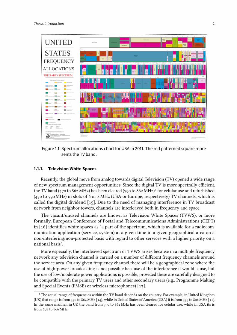
Moreover, it is not new that the electromagnetic spectrum is a scarce resource, beingalready fully occupied (or at least reserved for a certain kind of applications), see gure 1.11.Traditional spectrummarkets and static spectrummanagement originated a paradoxal situation:the spectrum is occupied without actually being used! Long-term licenses (for 15 years orlonger)—intended to prevent the various radio licensees from harmfully interfering with eachother—caused that in many areas the spectrum is being underutilized.
In fact, according to some measurement campaigns [11]–[13] in the range of 30MHz to3GHz, the maximum spectrum utilization is in general around 25 %, and the average use staysreally below that number. Thus, traditional markets cannot guarantee the ecient and exiblespectrum allocation.
1 http://www.ntia.doc.gov/files/ntia/publications/spectrum_wall_chart_aug2011.
1
Thesis Introduction 2
Figure 1.1: Spectrum allocations chart for USA in 2011. The red patterned square repre-
sents the TV band.
1.1.1. Television White Spaces
Recently, the global move from analog towards digital Television (TV) opened a wide rangeof new spectrum management opportunities. Since the digital TV is more spectrally ecient,the TV band (470 to 862MHz) has been cleared (790 to 862MHz)2 for celular use and refurbished(470 to 790MHz) in slots of 6 or 8MHz (USA or Europe, respectively) TV channels, which iscalled the digital dividend [15]. Due to the need of managing interference in TV broadcastnetwork from neighbor towers, channels are interleaved both in frequency and space.
The vacant/unused channels are known as Television White Spaces (TVWS), or moreformally, European Conference of Postal and Telecommunications Administrations (CEPT)in [16] identies white spaces as “a part of the spectrum, which is available for a radiocom-munication application (service, system) at a given time in a given geographical area on anon-interfering/non-protected basis with regard to other services with a higher priority on anational basis”.
More especially, the interleaved spectrum or TVWS arises because in a multiple frequencynetwork any television channel is carried on a number of dierent frequency channels aroundthe service area. On any given frequency channel there will be a geographical zone where theuse of high-power broadcasting is not possible because of the interference it would cause, butthe use of low/moderate power applications is possible, provided these are carefully designed tobe compatible with the primary TV users and other secondary users (e.g., Programme Makingand Special Events (PMSE) or wireless microphones) [17].
2 The actual range of frequencies within the TV band depends on the country. For example, in United Kingdom(UK) that range is from 470 to 862MHz [14], while in United States of America (USA) it is from 475 to 806MHz [11].In the same manner, in UK the band from 790 to 862MHz has been cleared for celular use, while in USA its isfrom 698 to 806MHz.
Thesis Introduction 3
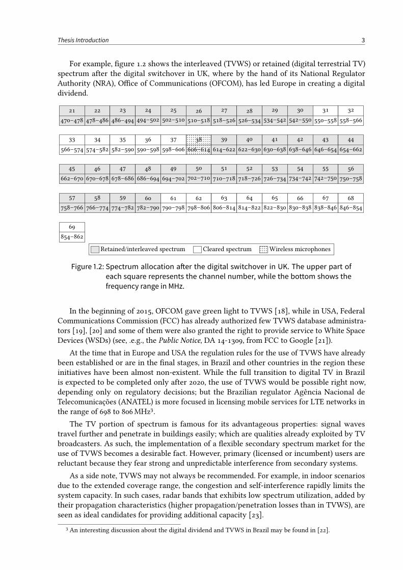
For example, gure 1.2 shows the interleaved (TVWS) or retained (digital terrestrial TV)spectrum after the digital switchover in UK, where by the hand of its National RegulatorAuthority (NRA), Oce of Communications (OFCOM), has led Europe in creating a digitaldividend.
21
470–478
22
478–486
23
486–494
24
494–502
25
502–510
26
510–518
27
518–526
28
526–534
29
534–542
30
542–550
31
550–558
32
558–566
33
566–574
34
574–582
35
582–590
36
590–598
37
598–606
38
606–614
39
614–622
40
622–630
41
630–638
42
638–646
43
646–654
44
654–662
45
662–670
46
670–678
47
678–686
48
686–694
49
694–702
50
702–710
51
710–718
52
718–726
53
726–734
54
734–742
55
742–750
56
750–758
57
758–766
58
766–774
59
774–782
60
782–790
61
790–798
62
798–806
63
806–814
64
814–822
65
822–830
66
830–838
67
838–846
68
846–854
69
854–862
Retained/interleaved spectrum Cleared spectrum Wireless microphones
Figure 1.2: Spectrum allocation aer the digital switchover in UK. The upper part of
each square represents the channel number, while the bottom shows the
frequency range in MHz.
In the beginning of 2015, OFCOM gave green light to TVWS [18], while in USA, FederalCommunications Commission (FCC) has already authorized few TVWS database administra-tors [19], [20] and some of them were also granted the right to provide service to White SpaceDevices (WSDs) (see, .e.g., the Public Notice, DA 14-1309, from FCC to Google [21]).
At the time that in Europe and USA the regulation rules for the use of TVWS have alreadybeen established or are in the nal stages, in Brazil and other countries in the region theseinitiatives have been almost non-existent. While the full transition to digital TV in Brazilis expected to be completed only after 2020, the use of TVWS would be possible right now,depending only on regulatory decisions; but the Brazilian regulator Agência Nacional deTelecomunicações (ANATEL) is more focused in licensing mobile services for LTE networks inthe range of 698 to 806MHz3.
The TV portion of spectrum is famous for its advantageous properties: signal wavestravel further and penetrate in buildings easily; which are qualities already exploited by TVbroadcasters. As such, the implementation of a exible secondary spectrum market for theuse of TVWS becomes a desirable fact. However, primary (licensed or incumbent) users arereluctant because they fear strong and unpredictable interference from secondary systems.
As a side note, TVWS may not always be recommended. For example, in indoor scenariosdue to the extended coverage range, the congestion and self-interference rapidly limits thesystem capacity. In such cases, radar bands that exhibits low spectrum utilization, added bytheir propagation characteristics (higher propagation/penetration losses than in TVWS), areseen as ideal candidates for providing additional capacity [23].
3 An interesting discussion about the digital dividend and TVWS in Brazil may be found in [22].
Thesis Introduction 4
Despite that, in a secondary spectrum market where channels, spectrum rights, andobligations are traded in a real-timemanner (and clearly stated by the NRA) alongwith (possible)WSDs’ sensing capabilities, geo-location database [18], [19], and spectrum broker [17], [24]should limit that fear of interference. Moreover, such market is also envisioned for other bandsof the spectrum [13].
1.1.2. Device-to-Device Communications
The scarcity of electromagnetic spectrum has also motivated the research of technologiesable to increase the capacity of wireless systems without requiring additional spectrum. Inthis context, Device-to-Device (D2D) communication (or broadly speaking, MTC) represents apromising technology.
D2D communication4 is a type of direct wireless communication between two or more net-work nodes, similar to direct-mode operation in professional mobile radio systems (colloquially,walkie talkies)5 or the bluetooth technology, that has attracted increasing attention of scienticcommunity in the last couple of years, mostly because of its deployment exibility [26]. D2Dcommunications can be implemented in Industrial, Scientic and Medical (ISM) bands forthe unlicensed spectrum use, such as Wireless Local Area Networks (WLANs), or in cellularnetworks for a licensed use [27].
Particularly, for communications happening in a cellular network (see gure 1.3), it isevidently resource inecient (both in terms of energy and bandwidth) to communicate viaa 3rd entity (cell tower) when nature provides a direct path between closely located networknodes [28]. Therefore, the main principle that underlays each D2D communication is toexploit the proximity of devices, which provides the hop gain (direct path), reducing energyconsumption, while allowing very high throughputs and low delays [27]. Moreover, the networkoperator does not need to be involved in the actual data transport (except for session setupsignaling, charging, and policy enforcement) [29], which ooads the core network; and at cellboundaries, D2D links may be used as relays to extend the coverage area [26], [30].
Reuse gain implies that radio resources can simultaneously be used by cellular and D2Dlinks, tightening the reuse factor (even for reuse-1 systems). The hop gain refers to the useof a single link in D2D mode rather than using Downlink (DL) and Uplink (UL) bands (inFrequency Division Duplex (FDD) systems) or dierent time slots (in Time Division Duplex(TDD) systems) like in cellular mode [26]. As a result, the overall system capacity and especiallythe spectral eciency is increased without requiring extra power from the battery of devices.
Thereby, due to their deployment exibility and aforementioned advantages, D2D commu-nications are currently being considered inside 3rd Generation Partnership Project (3GPP) tofacilitate MTC/proximity aware services, and security/public safety applications, becomingpart of LTE standards [31]. In this context, conventional cellular and D2D communicationsmay be respectively referred as primary and secondary communications.
However, the existence of D2D communication pose a new challenge: nodes and networkmust cope with new interference situations. For example, in cellular networks, the D2D linkscan reuse some of the already allocated physical resources [32]; and, in such case, the in-band(or co-channel) interference is no longer negligible because the orthogonality between links is
4 Sometimes also referred as Peer to Peer (P2P) communication.5 See the Trans European Trunked Radio Access (TETRA) standard [25].
Thesis Introduction 5
lost [33]. Moreover, the undesirable proximity of D2D and cellular transmitters/receiver maybring new types of inter-cell interference.
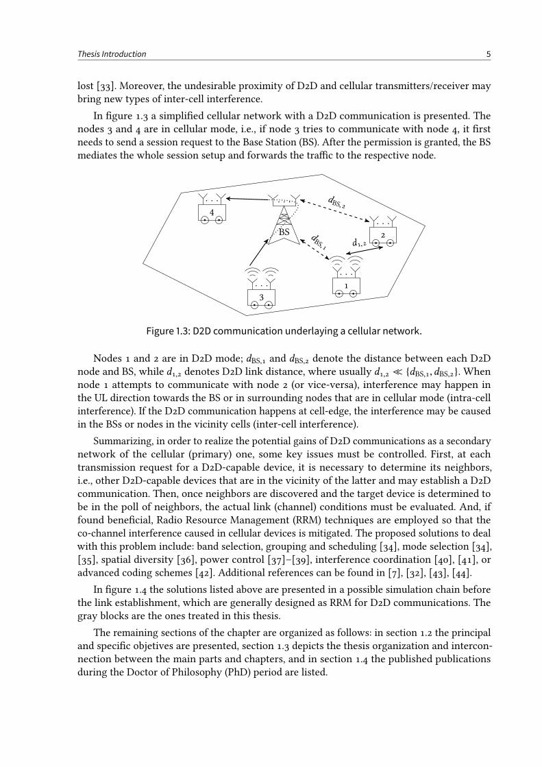
In gure 1.3 a simplied cellular network with a D2D communication is presented. Thenodes 3 and 4 are in cellular mode, i.e., if node 3 tries to communicate with node 4, it rstneeds to send a session request to the Base Station (BS). After the permission is granted, the BSmediates the whole session setup and forwards the trac to the respective node.
BS
. . .
1
. . .
2
. . .
3
. . .
4
. . .
d1,2dBS,1
dBS,2
Figure 1.3: D2D communication underlaying a cellular network.
Nodes 1 and 2 are in D2D mode; dBS,1 and dBS,2 denote the distance between each D2Dnode and BS, while d1,2 denotes D2D link distance, where usually d1,2 ≪ dBS,1,dBS,2. Whennode 1 attempts to communicate with node 2 (or vice-versa), interference may happen inthe UL direction towards the BS or in surrounding nodes that are in cellular mode (intra-cellinterference). If the D2D communication happens at cell-edge, the interference may be causedin the BSs or nodes in the vicinity cells (inter-cell interference).
Summarizing, in order to realize the potential gains of D2D communications as a secondarynetwork of the cellular (primary) one, some key issues must be controlled. First, at eachtransmission request for a D2D-capable device, it is necessary to determine its neighbors,i.e., other D2D-capable devices that are in the vicinity of the latter and may establish a D2Dcommunication. Then, once neighbors are discovered and the target device is determined tobe in the poll of neighbors, the actual link (channel) conditions must be evaluated. And, iffound benecial, Radio Resource Management (RRM) techniques are employed so that theco-channel interference caused in cellular devices is mitigated. The proposed solutions to dealwith this problem include: band selection, grouping and scheduling [34], mode selection [34],[35], spatial diversity [36], power control [37]–[39], interference coordination [40], [41], oradvanced coding schemes [42]. Additional references can be found in [7], [32], [43], [44].
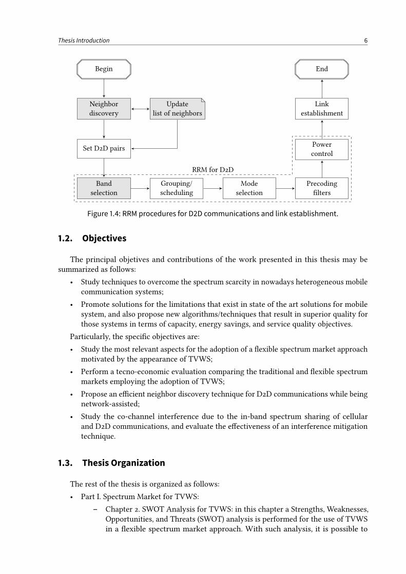
In gure 1.4 the solutions listed above are presented in a possible simulation chain beforethe link establishment, which are generally designed as RRM for D2D communications. Thegray blocks are the ones treated in this thesis.
The remaining sections of the chapter are organized as follows: in section 1.2 the principaland specic objetives are presented, section 1.3 depicts the thesis organization and intercon-nection between the main parts and chapters, and in section 1.4 the published publicationsduring the Doctor of Philosophy (PhD) period are listed.
Thesis Introduction 6
Begin
Neighbor
discovery
Set D2D pairs
Band
selection
Grouping/
scheduling
Mode
selection
Precoding
lters
Power
control
Link
establishment
End
Update
list of neighbors
RRM for D2D
Figure 1.4: RRM procedures for D2D communications and link establishment.
1.2. Objectives
The principal objetives and contributions of the work presented in this thesis may besummarized as follows:
• Study techniques to overcome the spectrum scarcity in nowadays heterogeneous mobilecommunication systems;
• Promote solutions for the limitations that exist in state of the art solutions for mobilesystem, and also propose new algorithms/techniques that result in superior quality forthose systems in terms of capacity, energy savings, and service quality objectives.
Particularly, the specic objectives are:
• Study the most relevant aspects for the adoption of a exible spectrum market approachmotivated by the appearance of TVWS;
• Perform a tecno-economic evaluation comparing the traditional and exible spectrummarkets employing the adoption of TVWS;
• Propose an ecient neighbor discovery technique for D2D communications while beingnetwork-assisted;
• Study the co-channel interference due to the in-band spectrum sharing of cellularand D2D communications, and evaluate the eectiveness of an interference mitigationtechnique.
1.3. Thesis Organization
The rest of the thesis is organized as follows:
• Part I. Spectrum Market for TVWS:
– Chapter 2. SWOT Analysis for TVWS: in this chapter a Strengths, Weaknesses,Opportunities, and Threats (SWOT) analysis is performed for the use of TVWSin a exible spectrum market approach. With such analysis, it is possible to
Thesis Introduction 7
identify the relevant aspects that may trigger the global adoption of TVWS and,as a consequence, foresee strategies to combat the resistance and promote thisnew market model;
– Chapter 3. Techno-Economic Evaluation for TVWS: in this chapter a detailedtecno-economic evaluation for the use of TVWS is explained. As use-case ex-amples three deployment scenarios are presented, considering the traditionaland exible market manners (2.60 GHz and 700MHz carriers, and 2.60GHzwith additional TVWS carrier, respectively) of a LTE network around a typicalEuropean city. Results show the potential money savings that operators mayreach if they adopt to use the TVWS in a exible market approach.
• Part II. D2D Communications:
– Chapter 4. Neighbor Discovery Using Power Vectors for D2DCommunications: inthis chapter it is proposed a network-assisted technique to discover D2D-capableneighbors of a rst Mobile Station (MS) based on the power measurementsalready available in the network. Results show that with the network help, thetime to detect all neighbors per MS is signicantly reduced, leaving more timeavailable for actual data transmission;
– Chapter 5. Band Selection for D2D Communications: in this chapter a novel co-channel interference mitigation algorithm is investigated. The algorithm selectsthe DL or UL band to be reused by the D2D communication using a radio distancemetric. Results proved that interference is mitigated in both communicationdirections, allowing the coexistence of cellular and D2D communication modes,which extends the common recommendation of just reusing the UL band for theD2D links.
• Chapter 6. Thesis Conclusion: this chapter gathers the most relevant conclusions of thethesis. At the end of the chapter some future works/research directions are highlighted.
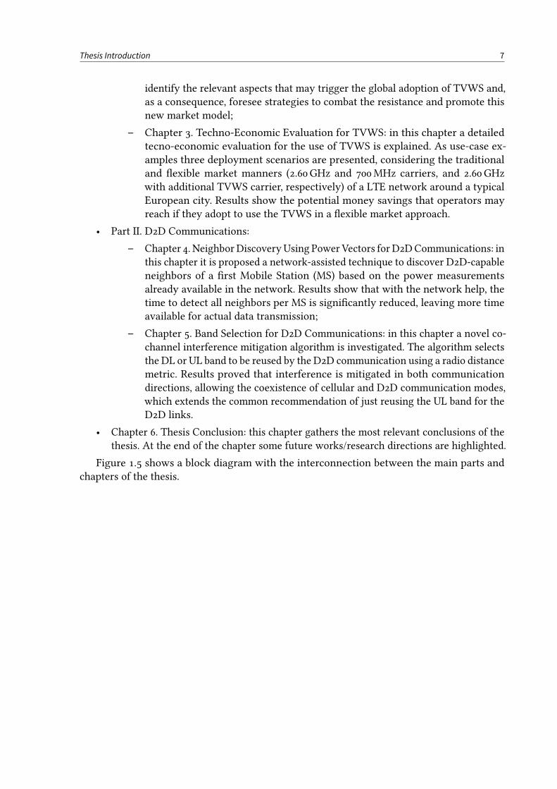
Figure 1.5 shows a block diagram with the interconnection between the main parts andchapters of the thesis.
Thesis Introduction 8
Spectrum Scarcity
Flexible SpectrumMarket
New SpectrumReuse Technique
Part I. SpectrumMarket for TVWS
• Chapter 2. SWOT Analysis forTVWS;
• Chapter 3. Techno-EconomicEvaluation for TVWS.
Part II. D2DCommunications
• Chapter 4. Neighbor DiscoveryUsing Power Vectors for D2DCommunications;
• Chapter 5. Band Selection forD2D Communications.
Figure 1.5: Block diagram for thesis organization.
1.4. Scientific Production
During the PhD period a few publications were issued as listed below. Those publicationsmay be divided in two general categories: main and related publications. The main publicationsserved as the basis for this thesis, while the related ones were written about correlated topicsin collaboration with colleagues.
1.4.1. Main Publications
These are the publications that served as the basis for the thesis:
1. C. F. Silva, H. Alves, and Á. Gomes, “Extension of LTE operational mode over TV whitespaces”, in Future Network and Mobile Summit 2011 Conference Proceedings, Warsaw,Poland, Jun. 2011, pp. 1–13. [Online]. Available: http://www.ict-cogeu.eu/pdf/publications/Y2/FUNEMS_2011_COGEU_paper_n2.pdf (visited on 10/2015);
2. C. Dosch, J. Kubasik, and C. F. M. Silva, “TVWS policies to enable ecient spectrumsharing”, in 22nd European Regional Conference of the International Telecommunications
Society (ITS 2011), Budapest, Hungary, Sep. 2011, pp. 1–26. [Online]. Available: http://hdl.handle.net/10419/52145 (visited on 10/2015);
3. C. F. M. Silva, F. R. P. Cavalcanti, and Á. Gomes, “SWOT analysis for TV white spaces”,Transactions on Emerging Telecommunications Technologies, vol. 26, no. 6, pp. 957–974,Jun. 2015, Published online: Dec. 2013, issn: 2161-3915. doi: 10.1002/ett.2770;
4. C. F. M. Silva, J. M. B. Silva Jr., and T. F. Maciel, “Radio resource management fordevice-to-device communications in long term evolution networks”, in Resource Alloca-
tion and MIMO for 4G and Beyond, F. R. P. Cavalcanti, Ed., New York, USA: SpringerScience+Business Media, 2014, pp. 105–156, isbn: 978-1-4614-8056-3. doi: 10.1007/978-1-4614-8057-0_3;
Thesis Introduction 9
5. C. F. M. e Silva and R. L. Batista, “Methods, nodes and user equipments for nd-ing neighboring user equipments with which a rst user equipment may be able tocommunicate directly”, P43774WO, Jul. 2014;
6. C. F. M. e Silva, T. F. Maciel, R. L. Batista, L. Elias, A. Robson, and F. R. P. Cavalcanti,“Network-assisted neighbor discovery based on power vectors for D2D communi-cations”, in IEEE 81st Vehicular Technology Conference (VTC 2015-Spring), May 2015,pp. 1–5, isbn: 978-1-4799-8088-8;
7. C. F. M. e Silva, R. L. Batista, J. M. B. Silva Jr., T. F. Maciel, and F. R. P. Cavalcanti, “In-terference mitigation using band selection for network-assisted D2D communications”,in IEEE 81st Vehicular Technology Conference (VTC 2015-Spring), May 2015, pp. 1–5, isbn:978-1-4799-8088-8;
8. C. F. M. e Silva and G. Fodor, “Method and system of a wireless communicationnetwork for detecting neighbouring UEs, of a rst UE”, P47887WO, Nov. 2015.
1.4.2. Related Publications
These are the related publications that were written in collaboration with colleagues:
9. R. L. Batista, C. F. M. e Silva, J. M. B. da Silva Jr., T. F. Maciel, and F. R. P. Cavalcanti,“Impact of device-to-device communications on cellular communications in a multi-cellscenario”, in XXXI Telecommunications Brazilian Symposium (SBrT2013), Fortaleza,Brazil, Sep. 2013. doi: 10.14209/sbrt.2013.241;
10. R. L. Batista, C. F. M. e Silva, J. M. B. da Silva Jr., T. F. Maciel, and F. R. P. Cavalcanti,“What happens with a proportional fair cellular scheduling when D2D communicationsunderlay a cellular network?”, in IEEE WCNC 2014 - Workshop on Device-to-Device and
Public Safety Communications (WCNC’14 - WDPC Workshop), Istambul, Turkey, Apr.2014, pp. 260–265;
11. R. L. Batista, C. F. M. e Silva, T. F. Maciel, and F. R. P. Cavalcanti, “Method and radionetwork node for scheduling of wireless devices in a cellular network”, P42550WO,Apr. 2014;
12. R. L. Batista, C. F. M. e Silva, J. M. B. da Silva Jr., T. F. Maciel, and F. R. P. Cavalcanti,“Power prediction prior to scheduling combined with equal power allocation for theOFDMA UL”, in Proceedings of 20th European Wireless (EW’14), Barcelona, Spain, May2014;
13. R. L. Batista, C. F. M. e Silva, T. F. Maciel, J. M. B. da Silva Jr., and F. R. P. Cavalcanti,“Joint opportunistic scheduling of cellular and D2D communications”, IEEE Transactionson Vehicular Technology, Submitted, issn: 0018-9545;
14. J. M. B. da Silva Jr., T. F. Maciel, R. L. Batista, C. F. M. e Silva, and F. R. P. Cavalcanti,“UE grouping and mode selection for D2D communications underlaying a multicellularwireless system”, in IEEE WCNC 2014 - Workshop on Device-to-Device and Public Safety
Communications (WCNC’14 - WDPC Workshop), Istambul, Turkey, Apr. 2014, pp. 230–235;
15. J. M. B. da Silva Jr., T. F. Maciel,C. F.M. e Silva, R. L. Batista, and Y. V. L. deMelo, “Spatialuser grouping for D2D communications underlying a multi-cell wireless system”,EURASIP Journal on Wireless Communications and Networking, Submitted, issn: 1687-1499;
Thesis Introduction 10
16. Y. V. L. de Melo, R. L. Batista, T. F. Maciel, C. F. M. e Silva, J. M. B. da Silva Jr., and F. R. P.Cavalcanti, “Power control with variable target SINR for D2D communications under-lying cellular networks”, in Proceedings of 20th European Wireless (EW’14), Barcelona,Spain, May 2014;
17. Y. V. L. de Melo, R. L. Batista, C. F. M. e Silva, T. F. Maciel, J. M. B. da Silva Jr., and F. R. P.Cavalcanti, “Power control schemes for energy eciency of cellular and device-and-device communications”, in IEEE Wireless Communications and Networking Conference
(WCNC’15), Mar. 2015, pp. 1690–1694. doi: 10.1109/WCNC.2015.7127722;
18. Y. V. L. de Melo, R. L. Batista, C. F. M. e Silva, T. F. Maciel, J. M. B. da Silva Jr., and F. R. P.Cavalcanti, “Uplink power control with variable target SINR for D2D communicationsunderlying cellular networks”, in IEEE 81st Vehicular Technology Conference (VTC 2015-
Spring), May 2015, pp. 1–5. doi: 10.1109/VTCSpring.2015.7146150;
19. A. R. F. de Oliveira, L. Elias, C. F. M. e Silva, T. F. Maciel e F. R. P. Cavalcanti,«Descoberta de vizinhos baseada em vetores de potência para comunicações D2D[Neighbor discovery based on power vectors for D2D communications]», em XXXIII
Telecommunications Brazilian Symposium (SBrT2015), Original document in Portuguese,set. de 2015, pp. 1–2.
1.4.3. Publications Summary
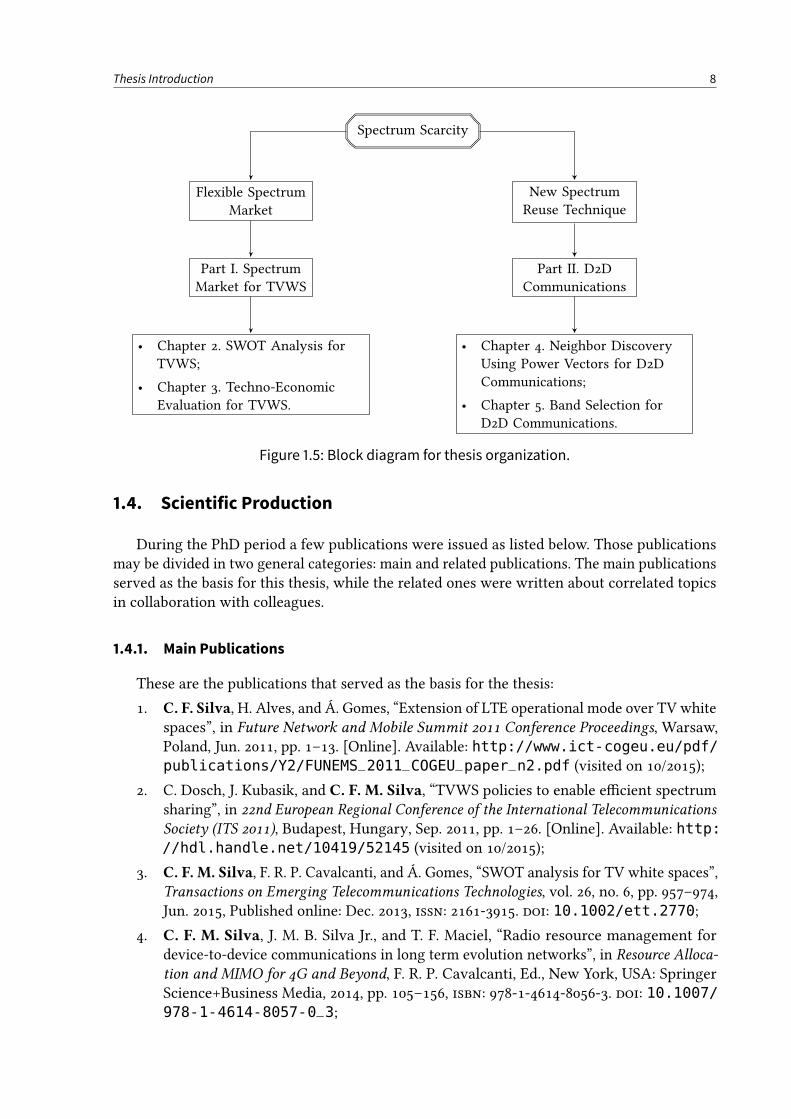
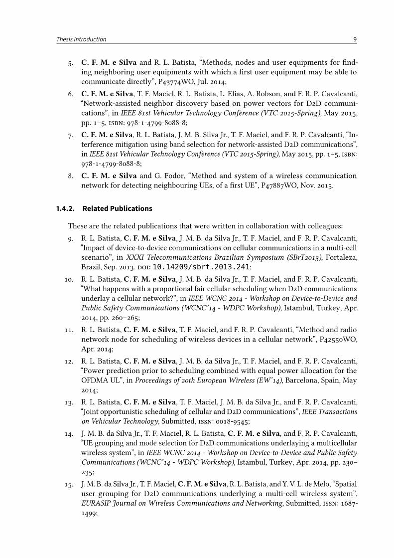
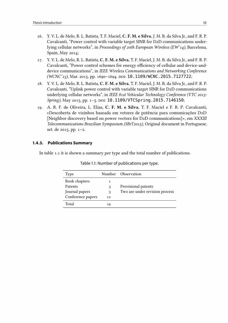
In table 1.1 it is shown a summary per type and the total number of publications.
Table 1.1: Number of publications per type.
Type Number Observation
Book chapters 1Patents 3 Provisional patentsJournal papers 3 Two are under revision processConference papers 12
Total 19
PART I
SpectrumMarket for TVWS
In this part the theme of Television White Spaces (TVWS) will be treated. The part is dividedinto the following chapters:
• Chapter 2. SWOT Analysis for TVWS: in this chapter a Strengths, Weaknesses, Oppor-tunities, and Threats (SWOT) analysis is performed for the use of TVWS in a exiblespectrum market approach. With such analysis, it is possible to identify the relevantaspects that may trigger the global adoption of TVWS and, as a consequence, foreseestrategies to combat the resistance and promote the new market model;
• Chapter 3. Techno-Economic Evaluation for TVWS: in this chapter a detailed tecno-economic evaluation for the use of TVWS is explained. As use-case examples, threedeployment scenarios are presented, considering the traditional and exible marketmanners (2.60 GHz and 700MHz carriers, and 2.60GHz with additional TVWS carrier,respectively) of a Long Term Evolution (LTE) network around a typical European city.Results show the potential money savings that operators may reach if they adopt to usethe TVWS in a exible market approach.
11
CHAPTER 2
SWOT Analysis for TVWS
The digital dividend will occur when the transition from analog to digital Television (TV)becomes eective. The freed and interleaved spectrum, known as Television White Spaces
(TVWS), may be a good opportunity for business related with new wireless services based onSoftware Dened Radio (SDR) and Cognitive Radio (CR) technologies. In this scope, the SWOT(Strengths, Weaknesses, Opportunities, and Threats) analysis—which helps in the identicationof inner (internal origin) and outer (external origin) factors of a company, service, or productthat characterize its position in the market—is considered a useful tool to evaluate the chancesof success for this new spectrum usage paradigm. In this chapter we present a suitable SWOTanalysis for the use of TVWS considering three dierent reference scenarios in the Europeancontext: spectrum of commons, secondary spectrum market, and prioritized services (publicsafety).
2.1. Introduction
The electromagnetic spectrum, when correctly managed, is an important catalyst for therapid development of economic (and social) activities through broadband wireless servicesprovision. Since the spectrum is considered a limited resource, its scarcity implies new usagestrategies and optimal allocation as collectively guided by regulatory, technical, and marketdomains. The current global switching from analog to digital TV has opened an opportunity tore-allocate this valuable resource [17], [60].
In one way, spectrum bands that are used for analog TV broadcasting will be cleared andreallocated to digital TV; but since the bandwidth required for digital TV is less than for theanalog, part of the spectrum will be freed up. In other way, to avoid interference betweenneighboring broadcasting stations, the spectrum bands are geographically interleaved, whichis known as TVWS. Roughly speaking, as presented in chapter 1, white spaces may be seen as“holes” in the spectrum that leave space for deploying new wireless services.
In this chapter we present a strategic positioning analysis of three scenarios (herein namedreference scenarios) regarding spectrum management in the TVWS context: (a) Spectrum ofcommons; (b) Real-Time secondary spectrum market; (c) And prioritized services. In all casesit is assumed that some kind of cognitive radio technology is in place for spectrum sensing,which allows its opportunistic use [61]–[63].
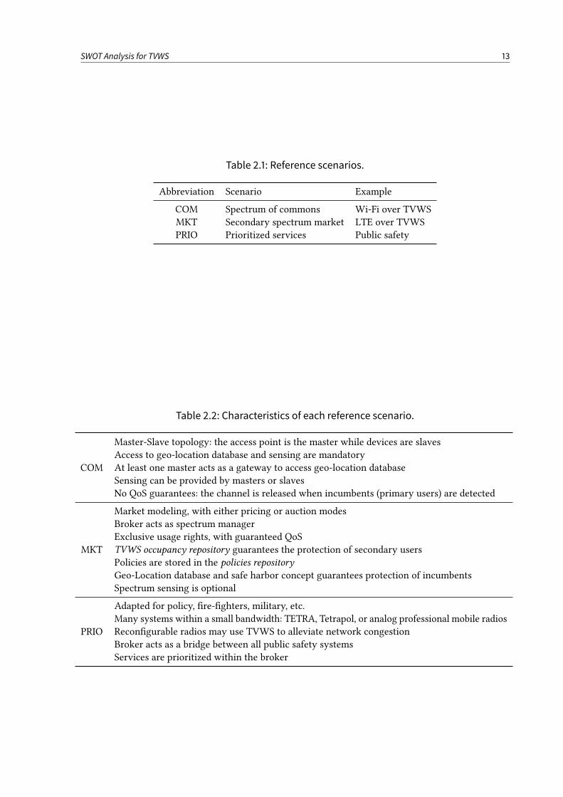
In table 2.1 it is presented each of the spectrum management scenarios with an applicabilityexample, while table 2.2 depicts their principal characteristics. These scenarios follow the de-scription that can be found in [24], [64] and are aligned with the European TelecommunicationsStandards Institute (ETSI) Recongurable Radio Systems (RRS) TR 102 907 document [60].
12
SWOT Analysis for TVWS 13
Table 2.1: Reference scenarios.
Abbreviation Scenario Example
COM Spectrum of commons Wi-Fi over TVWSMKT Secondary spectrum market LTE over TVWSPRIO Prioritized services Public safety
Table 2.2: Characteristics of each reference scenario.
COM
Master-Slave topology: the access point is the master while devices are slavesAccess to geo-location database and sensing are mandatoryAt least one master acts as a gateway to access geo-location databaseSensing can be provided by masters or slavesNo QoS guarantees: the channel is released when incumbents (primary users) are detected
MKT
Market modeling, with either pricing or auction modesBroker acts as spectrum managerExclusive usage rights, with guaranteed QoSTVWS occupancy repository guarantees the protection of secondary usersPolicies are stored in the policies repositoryGeo-Location database and safe harbor concept guarantees protection of incumbentsSpectrum sensing is optional
PRIO
Adapted for policy, re-ghters, military, etc.Many systems within a small bandwidth: TETRA, Tetrapol, or analog professional mobile radiosRecongurable radios may use TVWS to alleviate network congestionBroker acts as a bridge between all public safety systemsServices are prioritized within the broker
SWOT Analysis for TVWS 14
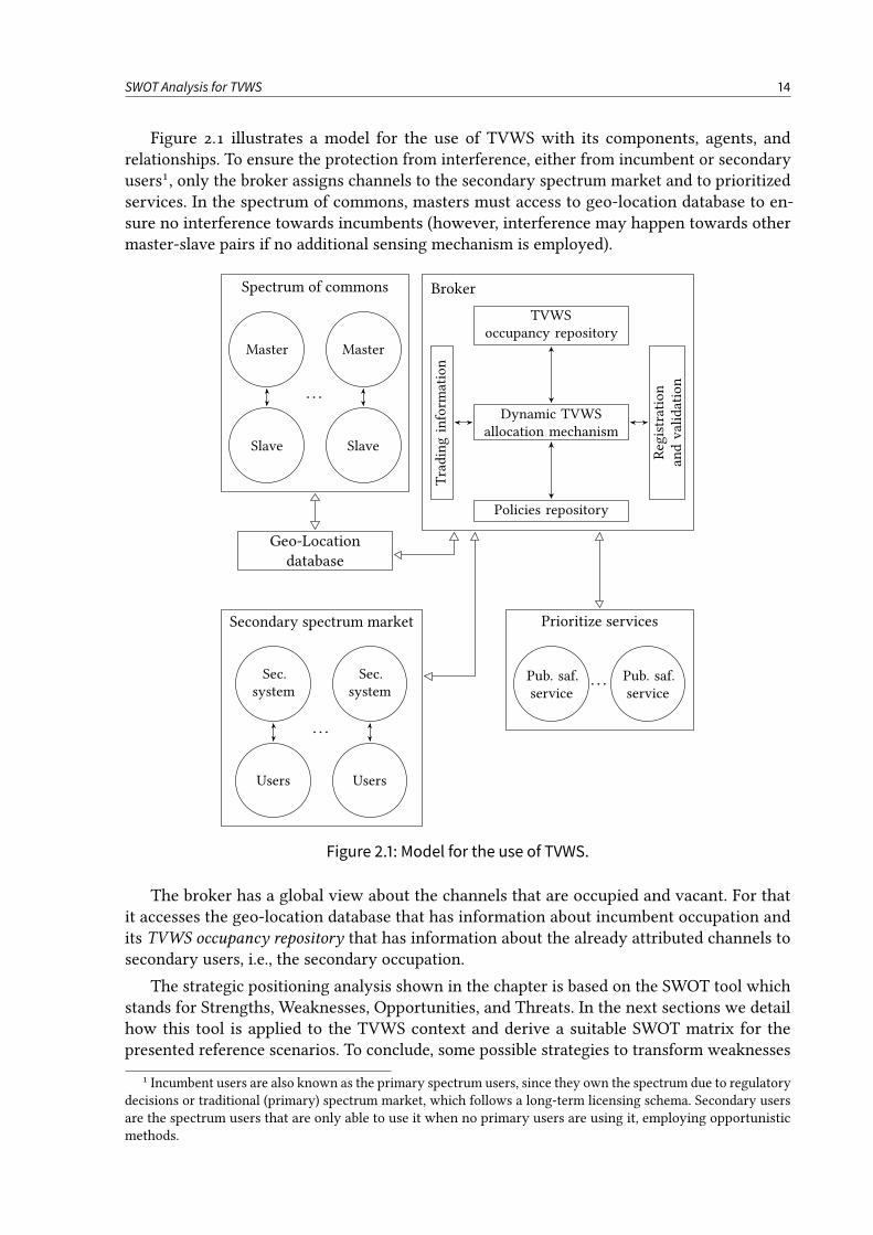
Figure 2.1 illustrates a model for the use of TVWS with its components, agents, andrelationships. To ensure the protection from interference, either from incumbent or secondaryusers1, only the broker assigns channels to the secondary spectrum market and to prioritizedservices. In the spectrum of commons, masters must access to geo-location database to en-sure no interference towards incumbents (however, interference may happen towards othermaster-slave pairs if no additional sensing mechanism is employed).
Master Master
Slave Slave
TVWS
occupancy repository
Tradinginform
ation
Dynamic TVWS
allocation mechanism
Registration
andvalidation
Policies repository
Geo-Location
database
Sec.
system
Sec.
system
Users Users
Pub. saf.
service
Pub. saf.
service
. . .
. . .
. . .
Spectrum of commons Broker
Prioritize servicesSecondary spectrum market
Figure 2.1: Model for the use of TVWS.
The broker has a global view about the channels that are occupied and vacant. For thatit accesses the geo-location database that has information about incumbent occupation andits TVWS occupancy repository that has information about the already attributed channels tosecondary users, i.e., the secondary occupation.
The strategic positioning analysis shown in the chapter is based on the SWOT tool whichstands for Strengths, Weaknesses, Opportunities, and Threats. In the next sections we detailhow this tool is applied to the TVWS context and derive a suitable SWOT matrix for thepresented reference scenarios. To conclude, some possible strategies to transform weaknesses
1 Incumbent users are also known as the primary spectrum users, since they own the spectrum due to regulatorydecisions or traditional (primary) spectrum market, which follows a long-term licensing schema. Secondary usersare the spectrum users that are only able to use it when no primary users are using it, employing opportunisticmethods.
SWOT Analysis for TVWS 15
in opportunities are discussed. Notice that while the present study is focused in the Europeancontext, the proposed methodology can be extended to other regions of the world.
2.2. SWOT Analysis Concept
In the time of economic crisis, a systematic reection about the chances of success for anew product2 assumes great importance. It is not only important the novelty in the solutionsthat the new product brings, but also a close view over external factors, such as the macroeconomic situation, market liquidity, or even the geographical area, may be the dierencebetween success or failure.
In this scope, the SWOT analysis is an integrated tool that allows companies to identifythe main inner (within the company) and outer (environmental) factors that characterize itsstrategic position in a certain moment regarding the whole market situation. However, its usemay not always be recommended, as it will be later discussed.
The SWOT analysis provides information that is helpful in matching the company’sresources and capabilities to the competitive environment in which it operates. As such, it isan instrument in the planning process, strategy formulation, and strategy selection.
The SWOT matrix, as shown in gure 2.2, is many times used as a visual tool for the SWOTanalysis. The matrix consists in two axis, each one composed by two variations: strengthsand weaknesses for the inner analysis; opportunities and threats for the outer analysis. Whilebuilding a matrix, the variables are some kind of overlapped, which facilitates the analysis anddecision-taking regarding the planning process.
Since the idea of the analysis is to determine the position of a company regarding a newproduct against its competitors, the SWOTmatrix presented in gure 2.3 becomesmore practical.As such, the SWOT analysis shall start with the clear denition of the objective, then variablesare identied and placed inside the matrix border cells at rows and columns as lists. Hence aquadrant is formed by the intersection of a row with a column. To make the analysis easierand normalized, herein we propose a scale of weights (which is not usually considered for theSWOT analysis) to be included in each variable. In the end, weights are summed in order toevaluate the relevance of each quadrant.
Depending on the prevalent variables, the product may fall into one of the four quadrants.In the rst quadrant strengths-opportunities (SO), maxi-maxi, the strategies shall focus themaximization of the outcomes since the strengths are in harmonywith themarket opportunities;this is clearly the expansion phase. In the second quadrant weaknesses-opportunities (WO),mini-maxi, the developed strategies shall overcome the weakness variables and, at the sametime, foresee the forthcoming opportunities; this is the growth phase. In the third quadrantstrengths-threats (ST), maxi-mini, the strategies shall be established in the way that strengthsminimize the eect of detected threats; this is a management phase. Finally, in the fourthquadrant weaknesses-threats (WT), mini-mini, the developed strategies shall try to minimizethe eects of weaknesses and market threats as much as possible; this is the survival phase [65].
After a careful analysis of the European mobile communications market and the technologybehind TVWS, we derive and analyze, in the following sections, a list of strengths, weaknesses,opportunities, and threats that are relevant for the three reference TVWS scenarios.
2 The term product is considered to be generic. It can designate a physical product, a project, a model, a service,or even an idea.

SWOT Analysis for TVWS 16
Helpfulto achieve the objective
Harmfulto achieve the objective
Internalorigin
productandcompanyattributes
Strengths WeaknessesExternalorigin
environm.andmarket
attributes
Opportunities Threats
Figure 2.2: General SWOTmatrix.
StrenghtsS1, S2, . . . , SN
WeaknessW1,W2, . . . ,WN
Opportunities
O1,O
2,...,ON
SO
ExpansionWO
Growth
Threats
T1,T2,...,TN
ST
ManagementWT
Survival
Internal origin
Externalorigin
Figure 2.3: Practical SWOTmatrix.
SWOT Analysis for TVWS 17
2.3. Strengths
Strengths include the positive internal factors. These are the qualities or trumps whichpositively distinguish the product in the market environment against the competition.
Roughly speaking, for the strengths detection, the sort of issues and questions which canbe addressed when using the SWOT analysis as part of business planning and decision-making,may be enumerated as follows [66]: (a) Advantages of the new product and its capabilities?(b) Unique Selling Point (USP), i.e., what dierentiates it from the concurrence? (c) What arethe main innovative aspects? (d) Financial reserves and likely returns? (e) Marketing: productannouncement, how to reach clients, and product distribution? (f) The price, additional values,and quality? (g) Accreditations, qualications, and certications? (h) Geographical location?(i) Current management and succession planning? (j) The product philosophy and its inheritedvalues?
In the context of this work, the strengths are discussed in the following paragraphs.
2.3.1. Flexible SpectrumUsage According to Regular User Needs
Applicable reference scenario: COM and MKT.
In the reference scenarios both the spectrum of commons and secondary spectrum tradingapproaches for TVWS are considered. In the spectrum of commons usage model, there isno spectrum manager (broker) to preside over the resource allocation. This regime promotessharing, but does not provide adequate Quality of Service (QoS) for some applications. However,for applications that require sporadic access to spectrum and for which QoS guarantees areimportant, temporary licensed spectrum with real-time secondary market may be the bestsolution. Trading allows players to directly trade spectrum usage rights with an appropriateService Level Agreement (SLA) between the seller and buyer, thereby establishing a secondarymarket for spectrum leasing and spectrum auction [67].
For the secondary spectrum market, it is important to stress that it has the potential to notjust open the market for new players but also to create new business opportunities for thespectrum broker entity either in the public or commercial sectors.
Of course, both regimes, spectrum of commons and secondary spectrum trading, are onlypossible to the extent allowed by National Regulator Authority (NRA) in each country.
2.3.2. Incumbent Users Are Able to Resell Their Unused Spectrum
Applicable reference scenario: MKT.
Within the concept of secondary spectrum market, the incumbent (or primary) users shallbe able to resell their unused spectrum to the broker and be paid for that. This spectrum willlater enter in the secondary spectrum market for reselling. Therefore, not only the optimizationin the spectrum usage is achieved, but also money incoming for incumbents.
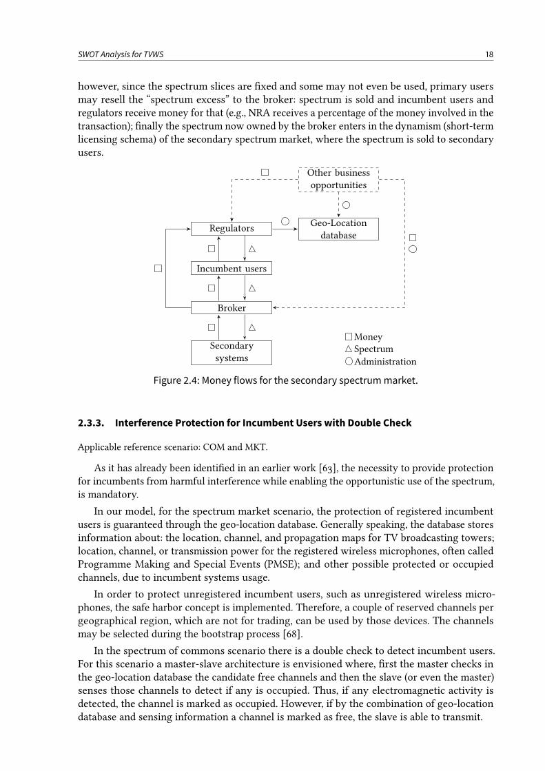
In gure 2.4 the envisaged money ows are depicted: the regulator is responsible to managethe spectrum. As such it administrates the geo-location database and/or may outsource themanagement of the database to a company, therefore creating new business opportunities (thesame applies to the broker); on the other hand, NRA promotes the primary spectrum market(with exclusive access rights) for incumbent users: the spectrum is sold and money received;
SWOT Analysis for TVWS 18
however, since the spectrum slices are xed and some may not even be used, primary usersmay resell the “spectrum excess” to the broker: spectrum is sold and incumbent users andregulators receive money for that (e.g., NRA receives a percentage of the money involved in thetransaction); nally the spectrum now owned by the broker enters in the dynamism (short-termlicensing schema) of the secondary spectrum market, where the spectrum is sold to secondaryusers.
Secondary
systems
Broker
Incumbent users
RegulatorsGeo-Location
database
Other business
opportunities
Money
Spectrum
Administration
Figure 2.4: Money flows for the secondary spectrummarket.
2.3.3. Interference Protection for Incumbent Users with Double Check
Applicable reference scenario: COM and MKT.
As it has already been identied in an earlier work [63], the necessity to provide protectionfor incumbents from harmful interference while enabling the opportunistic use of the spectrum,is mandatory.
In our model, for the spectrum market scenario, the protection of registered incumbentusers is guaranteed through the geo-location database. Generally speaking, the database storesinformation about: the location, channel, and propagation maps for TV broadcasting towers;location, channel, or transmission power for the registered wireless microphones, often calledProgramme Making and Special Events (PMSE); and other possible protected or occupiedchannels, due to incumbent systems usage.
In order to protect unregistered incumbent users, such as unregistered wireless micro-phones, the safe harbor concept is implemented. Therefore, a couple of reserved channels pergeographical region, which are not for trading, can be used by those devices. The channelsmay be selected during the bootstrap process [68].
In the spectrum of commons scenario there is a double check to detect incumbent users.For this scenario a master-slave architecture is envisioned where, rst the master checks inthe geo-location database the candidate free channels and then the slave (or even the master)senses those channels to detect if any is occupied. Thus, if any electromagnetic activity isdetected, the channel is marked as occupied. However, if by the combination of geo-locationdatabase and sensing information a channel is marked as free, the slave is able to transmit.
SWOT Analysis for TVWS 19
The sensing information complements the geo-location database both in time and space,therefore a more ne-grained information is obtained. In fact, the combination of both infor-mation sources is seen as a more accurate method to protect incumbent users and avoid, e.g.,the so-called hidden node problem [69].
2.3.4. QoS with Interference Protection for Secondary Users
Applicable reference scenario: MKT.
Inside the broker, the TVWS occupancy repository ensures that all secondary users areregistered in the database, and the channels that were attributed to them in a previous tradingprocess are marked as occupied. When the market opens, only the free channels are subject oftrading. Moreover, a SLA is established between the player and the broker, which enforces therequired QoS.
2.3.5. Prioritized Services and Interconnection
Applicable reference scenario: PRIO.
Within the broker, services are prioritized according to their type. In emergency situations,the network would be in the emergency mode. In such case, all public safety services areprioritized over any other service.
The higher priority of services in the access of TVWS is done by implementing an adequateset of policies that are stored in the policies repository inside the broker.
Apart from prioritizing, the broker may also act as a bridge to interconnect all the publicsafety systems and set a couple of restricted TVWS channels to alleviate congestion within thealready existent public safety shared band.
2.3.6. The Implementation and Management of Geo-Location Database
Applicable reference scenario: COM and MKT.
Besides spectrum-sensing capabilities, in [70] the Federal Communications Commission(FCC) clearly states that White Space Devices (WSDs)—SDR and CR devices that operate inTVWS—must access a database to determine the free available channels. In this sense, all WSDsfor the foreseeable future are going to use a geo-location database to avoid interference withlicensed spectrum users.
In 2009, FCC issued a public notice inviting proposals for TV band device database managers.In the beginning of 2011, FCC conditionally designated nine companies as administrators for awhite spaces database and outlined some important ground rules for its operation [19].
Taking the FCC as an example, we consider that multiple geo-location database admin-istrators or multiple spectrum brokers would bring new players to the market, creating acompetitive environment where policies against market abuse apply.
2.3.7. Competition and Innovation
Applicable reference scenario: COM, MKT, and PRIO.
SWOT Analysis for TVWS 20
A secondary spectrum market with temporary exclusive rights allows small players togo to the market and request (or place their bids) for spectrum. With this new concept ofspectrum trading, the market is more dynamic and the granted rights are for short-term use.Therefore, small companies (e.g., hotels, associations, festivals, etc.) that require extra capacityfor a specic period in time may compete with big companies for the selling spectrum.
Herein we shall also consider SDR and CR devices, e.g., with sensing capabilities and GlobalPositioning System (GPS) transceivers, let’s say the future WSDs. However, they must be seenas more a futuristic opportunity to be developed in longer term.
2.3.8. Transparent Market with Real-Time Information
Applicable reference scenario: MKT.
The introduction of spectrum trading relies on making available to the public all informationrelated with the spectrum usage (existing spectrum ownership, individual trades, area andpopulation coverage, technologies, services and applications, spectral eciency, etc.). Regardingthis issue, there should be a strong support by the national authorities in order to provideonline registries, including the information about license conditions, rights and obligations(e.g., through a Web service).
2.3.9. Flexibility in Building on Demand Networks
Applicable reference scenario: COM and MKT.
The exibility is related with channel (or carrier) assignment. As it was already discussed,three reference scenarios are envisaged: COM, MKT, and PRIO (see table 2.1). While PRIOis related with prioritizing services and its use is mainly concerned with public safety, theother two (COM and MKT) are tailored for common use and may coexist both in time andspace: if secondary user does not require QoS, it should select COM; otherwise, and if QoS is arequirement, then MKT shall be followed.
2.3.10. A Better Management of Costs: CAPEX Becomes OPEX
Applicable reference scenario: MKT.
Broadly speaking, Capital Expenditure (CAPEX) is something you want to avoid, whileOperational Expenditure (OPEX) is something you want to keep under control. In commonbusiness parlance, CAPEX is taken to mean upfront cash outlays for an asset depreciatedover time (i.e., the initial investment), and OPEX as general run operating expenditures (i.e.,maintenance costs).
Not having to pay an upfront cost may be seen as an important aspect. However, the benetsof payments over time can be erased by situational issues, e.g., money valorization, interestrates, or rental fees. Therefore, there is nothing inherently nancially benecial to switch froman upfront investment to cash outlay overtime.
Nevertheless, with any activity which is highly variable and has large capacity spikes, therecan be a huge benet to switching from an upfront investment covering the maximum ofcapacity over the whole time period to variable pricing based upon actual activity. Seasonal
SWOT Analysis for TVWS 21
capacity spikes in many businesses can be an order or more of magnitude from base levels ofactivity.
With the secondary spectrum market, players are encouraged to request TVWS on atemporary basis. The most illustrative example is the case of a Long Term Evolution (LTE)operator who wants to mitigate the lack of capacity in its network during the peak hours (or ina certain region during, e.g., summer time) and uses TVWS to overcome that situation. In suchcase, the acquisition of spectrum for just few hours or days would be highly benecial.
2.3.11. Support from Broadcasters Due to Interference Limitation
Applicable reference scenario: COM, MKT, and PRIO.
Broadcasters fear the interference that may be caused by mobile systems if TVWS enterin the regular spectrum market. For this cause, the ideas defended in this work, namelythe implementation of interference protection ratios that limit the interference caused bysecondaries in incumbent systems is seen more than welcome.
Nevertheless, their concern is that WSDs shall not block the evolution of Terrestrial DigitalVideo Broadcast (DVB-T) technology.
2.4. Weaknesses
The weaknesses of the project include the negative internal factors. They are consideredsuch as limiting the eciency aspects. In order to identify the potential weaknesses of theproject the following criteria may apply [66]: (a) Disadvantages of the new product? (b) Gapsin capabilities and known vulnerabilities? (c) Lack of competitive strength? (d) Past historyreputation and adopted strategies to reach clients? (e) Financial issues in cash ow and start-upcash-drain? (f) Timescales, deadlines, and pressures? (g) Continuity, supply chain robustness?(h) Eects in the core activities and possible distractions?
In this work the considered weaknesses are presented in the next paragraphs.
2.4.1. Eective Real-Time Market: Pricing and Auction Modes
Applicable reference scenario: MKT.
In order to implement the secondary spectrum market, a real-time market with ecientdispute resolution mechanisms is required. Therefore, denitions like the market opening time,notication of players (e.g., which kind of information shall be exchanged and how), preemptivevs. non-preemptive formulation, etc. [71] must be clearly stated.
Moreover, the broker supports both pricing mode, when the oer is greater than thedemands, and auction mode, when the demands are greater than the oer [24], [64]. In thepricing mode, the seller determines a xed price for the spectrum and the buyer simply paysthe stipulated price. In the auction mode, the seller xes a benchmark price and buyers placetheir bids for the auctioned band; the winning bid decides the nal price. However, a successfulauction requires that players have a clear understanding about the rights and obligations thatare imposed on them, especially to the winner; if there is uncertainty about these issues, it willdiscourage competitive bidding [71]. Through the negotiation protocols, the broker maximizesits revenues as well as ensures fairness between players.
SWOT Analysis for TVWS 22
The spectrum is sold in terms of rst come rst served basis in the pricing approach, orthe most valuable bidder wins the band depending on the auction mechanism. However, theprocess of determining the most valuable bidder (in real-time) is seen as a NondeterministicPolynomial Time (NP) problem [72]. Therefore, sophisticated and computationally-intensivemodels shall be used, which may jeopardize the real-time market.
2.4.2. Traditional SpectrumMarket Is Easier to Implement
Applicable reference scenario: MKT.
The traditional market is usually implemented by a non-real-time auction process thathappens during a period of time, e.g., a couple of months [73]. It may be done in a single roundof bids for the spectrum bands or with a multi-round of bids (which was the Portuguese case inrecent spectrum auctions [74]).
Thus, and because real-time decisions are not required and the exclusive usage rights arefor long-term periods (15 or 20 years), this market model is easier to implement.
2.4.3. LowMarket Liquidity
Applicable reference scenario: MKT.
One of the main concerns for the implementation of a secondary spectrum market is thelow market liquidity, for instance due to a limited number of players competing for spectrumin a given area.
In this work we consider as a use case the extension of LTE over TVWS, for the secondaryspectrum market reference scenario (MKT). If we assume that most of the use of TVWS comesfrom LTE network operators and if we consider three or four LTE operators per country andif, as expectable its TVWS allocations are medium to long-term, the market will not be verydynamic.
On other hand, it should be pointed out that our model allows small players to enter inthe spectrum market, buying spectrum for temporary use such as telemetry applications,Machine-to-Machine (M2M) applications or Wireless Fidelity (Wi-Fi)-like applications withQoS guarantee. Thus, Wi-Fi network operators would benet from entering secondary marketinstead of spectrum commons (COM).
2.4.4. Rules Against Monopolization and Market Abuse
Applicable reference scenario: MKT.
The NRA shall promote the ecient utilization of the spectrum while creating conditionsfor new players to come into the market [75]. Therefore, and in order to avoid monopolization,a limiting process for the spectrum ownership shall be implemented [63], e.g., by spectrum
caps [73], [74] or other means.
Maximizing the opportunities for the spectrum-using industry requires that spectrum isfully and eciently used, and no company is able to hoard or use market power in spectrumlicenses with the eect of foreclosing or limiting the competition among players [76].
SWOT Analysis for TVWS 23
Policies are described inside the broker, namely they are implemented in the policies
repository [71]. Its omission, bad denition, or malfunction implementation may underminethe secondary market.
2.4.5. Security: Authentication, Validation, and Blacklisting of Players
Applicable reference scenario: MKT.
In the secondary spectrum market, a security mechanism is necessary to protect messagestransmitted between each player and the broker, like control messages to request or assignTVWS channels, update information about the market, etc. In addition, between the brokerand geo-location database a secure path may be assumed.
The importance of security can be summarized (at least) for the following situations:
(a) Since our model assigns TVWS channels and the spectrum is a scarce resource,security attacks may lead to spectrum’s occupancy from those who are not authorized;
(b) In the secondary spectrum market, fake entities would request more TVWS channelsand possibly resell them, building a parallel illegal market;
(c) Fake entities would notify players as being the broker, and then collect money for thespectrum and spectrum rights that they do not own.
However, no esoteric security mechanisms seem to be necessary; simple and standardizedmechanisms, such as the asymmetric cryptographic (or public-key cryptography) may besucient [64].
Moreover, the broker shall be able to shut down those WSDs that are deemed to bemisbehaving. Hence, a blacklisting functionality can be built to dissociate an oending clientand prevent it from re-associating with the network [77].
2.4.6. Compute the TVWSMaps
Applicable reference scenario: COM and MKT.
The process of building TVWS maps to be stored in geo-location database is not a simpletask. It is based on propagation loss models that are adapted according to the geographical areaand scenario under study [78].
The computation of those maps can be very intensive and to achieve a satisfying accuracy,complex and sophisticated models shall be used. In such case, the waste of white spaces islow [77].
However, more simplistic and less computationally intensive models and/or conservativevalues for the model parameterization may also be used, but with a higher percentage of wastedwhite spaces, therefore with less satisfactory results.
2.4.7. Cross Border Issues in Interference Control and SpectrumHarmonization
Applicable reference scenario: COM, MKT, and PRIO.
Spectrum harmonization, where countries across a region use the same spectrum frequency,is vital [79]. It is critical for the successful and cost-eective deployment of any wireless service
SWOT Analysis for TVWS 24
as it provides the economies of scale, which drive down the costs of devices and of the networkitself, while encouraging innovation [80].
Without harmonization, the interference in these regions is predictably high [15], [79],which does seriously limit the QoS or Quality of Experience (QoE). In such case, one of followingsituations may happen: either the prices of devices are aordable, but due to interference levelthey cannot properly operate, or the costs of devices are prohibitively high (e.g., becausesuperior narrow lters are necessary), which probably reduces their uptake. In both situations,it would harm not only consumers and the mobile industry, but also reduce the benets thatmobile technologies bring to national economies.
2.4.8. Hidden Node Problem
Applicable reference scenario: COM, MKT, and PRIO.
The hidden node happens when the incumbent signal (let’s say DVB-T or PMSE signals) isnot properly detected by the CR device due to buildings or trees, with partial or full blockage [69],[81]. Due to the dierent spatial conditions, the device erroneously detects no transmission inthe current channel and no nearby receiver, thus the channel is marked as vacant. In this case,any secondary transmission on such channel would cause harmful interference to incumbentusers.
In order to overcome the hidden node problem, the use of correct signal strength detectionthresholds and/or the combination of sensing and geo-location database information must becorrectly implemented.
2.4.9. Communication With the Geo-Location Database and Location Accuracy
Applicable reference scenario: COM and MKT.
For the secondary spectrum market, MKT, we foresee the use of sensing as optional, but theaccess to the geo-location database is mandatory; while for the spectrum of commons, COM,both geo-location information and sensing are mandatory. Therefore, a reliable communicationbetween the broker and geo-location database is required, not only due security issues in theexchange of sensible data, but also to ensure that the broker has the latest updated version ofTVWS maps.
On the other hand, a white spaces network for which the WSDs rely on a database, needsto ensure that its users know their correct location when it comes the time to request a TVWSchannel. At rst glance, it may be not obvious why clients need to be equipped with locationinformation, because a comprehensive map [77] could be elaborated with the information ofevery single point within the coverage area of each Base Station (BS). However, this methodcan result in losses about the amount of available white space channels, as the maps result fromthe union of all occupied channels within the coverage area of BS. Thus, while requesting achannel, if the user’s location information is provided, a more ne-grained regional informationis provided and therefore the detection of available channels is more accurate and reliable.
Moreover, in such architecture any change in the spectrum occupancy by incumbent usersmust be disseminated to the secondary clients at their respective locations with very lowlatencies; or WSDs periodically query the database to learn the available white spaces [77]. Inthe case of TVWS occupancy repository inside the broker, the same procedure may also apply.
SWOT Analysis for TVWS 25
2.5. Opportunities
Opportunities are positive external factors that can be seen as targets to achieve or tenden-cies to be exploited in the future which, when used in appropriate manner, will be an impulsefor the development or for weakening the threats.
Some of the questions that may be answered in order to identify the market opportunitiesare listed below [66]: (a) Global inuences, industry, or lifestyle trends? (b) Technologicaldevelopment and innovation? (c) Global or niche target market developments, e.g., new verticalor horizontal markets? (d)Market response to tactics, e.g., surprise? (e)Market volume demands?(f) Competitors’ vulnerabilities? (g) Partnerships, major contracts, agencies, and distribution toreach clients? (h) Geographical area, exportation, and importation? (i) Tendencies: seasonal,weather, and fashion inuences?
In this work the external factors that may positively inuence the product’s outcomes aredescribed in the following paragraphs.
2.5.1. TVWS Stability
Applicable reference scenario: COM, MKT, and PRIO.
The TVWS stability depends mainly on the power levels of TV broadcasters after thebroadcast frequencies plan had been established and approved by the NRA. Both the broadcastplan and the power levels are stable, thus TVWS are also stable. In the case of unregisteredwireless microphones, PMSE, the safe harbor concept (i.e., reserved and not tradable channels)may be used, therefore, not causing harmful interference.
2.5.2. Geographical Dependence of TVWS
Applicable reference scenario: COM, MKT, and PRIO.
The TVWS refers to the cleared and geographical interleaved electromagnetic spectrumthat will be freed up after the digital TV switchover (or analog TV switch-o) is completed.The amount of cleared spectrum is known as digital dividend [68].
The TVWS geographical dependence brings many benets, e.g., the possibility of harmo-nized frequencies, the balanced allocation of spectrum between dierent service providers, andthe avoidance of interference within the boundaries of the European Union [15].
The European Union issued the document [82], which presents a couple of directives tomake spectrum market more exible and harmonized between the member states, which isclearly an opportunity to seek for new TVWS markets, being in line with the Europe 2020initiative and the Digital Agenda for Europe.
2.5.3. Service Availability and Broadband Services in Remote Areas
Applicable reference scenario: COM, MKT, and PRIO.
The TVWS are localized within the Ultra High Frequency (UHF) band3, namely in the 470 to790MHz band [68]. This spectrum band oers excellent balance between transmission capacity
3 The UHF band ranges from 300MHz to 3GHz.

SWOT Analysis for TVWS 26
and distance to cover. Because of its good signal propagation characteristics, less infrastructureis required to provide wider mobile coverage, meaning that (broadband) communication servicescan be provided in rural areas at lower cost, which would bring a benecial social impact.
Moreover, and since rural places are not densely populated places, the availability of TVWSis higher than in urban areas allowing a bigger number of dierent telecommunication solutionswithout causing interference.
2.5.4. Coverage and Enhanced Indoor Services
Applicable reference scenario: COM, MKT, and PRIO.
Lower frequencies suer less propagation losses, as well as, lower penetration losses throughwalls. Therefore, with the use of TVWS a new variety of indoor services can be provided, namelyin urban areas.
Overall, this would lead to faster, cheaper, and better services with an increased possibilityfor content enhancement and interoperability of devices (e.g., mobile TV).
2.5.5. Simplifying Spectrum Trading and Positive Examples fromOther Countries
Applicable reference scenario: MKT.
Following the initial assignment of spectrum rights and obligations to users, whether byauction or other means, circumstances may change causing initial license holders to want totrade their rights and obligations with others. Nowadays this is not possible in many countries.However, in a few countries, the secondary trading—trading of spectrum rights after the primaryassignment—is possible. Examples from other countries are a critical factor in the promotion ofmore ecient radio spectrum use. Furthermore, it is increasingly recognized that the exibilityaorded by trading is helpful for innovation and competitiveness [71].
Regarding this topic, in United Kingdom, Oce of Communications (OFCOM) has publisheda report [83] where the simplication of spectrum trading process is discussed and encouraged.This example may be followed by other countries, even outside the European zone.
2.5.6. Super Wi-Fi Concept Proposed by FCC
Applicable reference scenario: COM.
Super Wi-Fi is a term coined by FCC to describe a wireless networking proposal for thecreation of longer-distance wireless connections [70].
Instead of using the 2.40GHz radio frequency of regular Wi-Fi, the Super Wi-Fi proposaluses the TVWS channels to transmit Wi-Fi signals. These lower frequencies allow the signal totravel further and penetrate walls better than higher frequencies, which overcomes the shortrange problem of traditional Wi-Fi networks. The plan of FCC is to allow those white spacefrequencies to be used for free, as it happens with regular Wi-Fi.
With Super Wi-Fi, it is possible to create larger Wi-Fi networks to replace the presenthotspots and companies would see their consumers oered with extensive and high-speedWi-Fi services for cheaper prices.
SWOT Analysis for TVWS 27
Regarding this issue, objections may come from broadcasters and wireless microphone com-panies. However, with the implementation of protection ratios, broadcasters and microphoneusers shall feel safer.
2.5.7. Backhaul over TVWS
Applicable reference scenario: MKT and PRIO.
In LTE release 8, the predicted downlink theoretical throughput peak rates may reach upto 300Mbit/s per BS with 4 × 4 Multiple Input, Multiple Output (MIMO) [84], which requiresnew backhaul4 strategies in order to deliver cost eective networks.
The choice of optical ber seems natural since it can deliver almost unlimited bandwidths.While it is true for mobile operators that have already installed their own ber connectionbetween the access network and core network (which may be reused from their previousnetworks), it may not be the case for an operator that does not own a ber connection andmust lease it from a third-party, or build out a new ber plant.
For the latter case, a microwave link may be seen as an alternative. A microwave link(including the installation and lifetime operation) can be three to ve times cheaper than anEthernet link and almost 10 times cheaper than the ber link for urban and sub-urban areas [85].
Microwave technology has evolved and solutions using multi-carrier and MIMO techniquesmay notably increase the downlink throughput peak rate up to 1.60Gbit/s per link [85], whichis comparable with the one achievable using optical ber. The previous downlink throughputpeak rate is likely to be achieved with a bandwidth of 50MHz, which can be obtained employingcarrier aggregation (see section 2.5.10). Moreover, advances in modulation technology andsignal processing promise to increase capacity in the near future.
Due to excellent propagation characteristics of lower frequencies and in times where theavailable spectrum is scarce, the use of TVWS for backhaul links, especially in MKT scenario,may be seen as an alternative.
2.5.8. The Needs of Bandwidth over the Next Years
Applicable reference scenario: COM and MKT.
In 2011 the global mobile data trac increased 133 % [86], with respect to previous year andthis increase is predicted to continue over next several years [1], [86]. The key drivers in thisrapid growth are related with the maturity of already deployed networks, such as Wi-Fi andHigh Speed Packet Access (HSPA), and the roll-out of new mobile technologies, namely, LTE.Moreover, the popularity of Wi-Fi-enabled devices, such as smartphones and tablets, boomedthe network trac. For the next decades, a huge increase in the M2M wireless communicationsis also expected [1], [87].
The need of electromagnetic spectrum to fulll the above demands for wireless broadbandservices is evident. For this purpose, the use of TVWS along with WSDs is already a subjectunder study by some NRA, such as FCC [70] and OFCOM [88].
Additionally, in World Radiocommunication Conference (WRC)-07 it had already beenidentied, according to International Telecommunications Union (ITU)’s system of regional
4 In a hierarchical telecommunications network the backhaul portion of the network comprises the intermediatelinks between the core (or backbone) network and the access network.
SWOT Analysis for TVWS 28
classication, the following blocks of digital dividend: 72MHz for Europe/Africa (Region 1)and Asia/Oceania (Region 3), and 108MHz for Americas (Region 2) and some countries inAsia/Oceania (Region 3). However, the mobile industry considers these identications to bethe minimum amount required in each region, and states that a larger bandwidth shouldbe cleared—at least 100MHz per each region—, which represents approximately 25 % of thespectrum allocated for terrestrial broadcasting after the digital TV switchover [80].
Moreover, operators also claim that more spectrum (i.e., more licensed channels) wouldbring more players into the telecommunications market, diversifying the oer of new productsand, at the same time, lowering their prices.
2.5.9. More Eicient Use of Electromagnetic Spectrum
Applicable reference scenario: MKT.
A market-based approach for spectrum management might be considered as a way toimprove the ecient use of the radio spectrum [67]. This mechanism would imply that under-utilized spectrum assets could be transferred to individuals or organizations, deriving in greatereconomic returns from their use. In this way, it would lead to an enhanced use of the radiospectrum [24], [64].
Moreover, new enhancements in technology allow the coexistence of dierent radiotechnologies in a relative small portion of the spectrum. This can be more related withLTE because of its exibility to operate in dierent contiguous bandwidths. The 1.40MHz,3MHz, and 5MHz bandwidths that were specied in the LTE release 8 can be accommodatedwithin the 8MHz bandwidth of a DVB-T channel. However, if higher bandwidths (10MHz,15MHz, or 20MHz, also specied in the same LTE release) are required, dierent contiguousor non-contiguous DVB-T channels can be aggregated to provide the total bandwidth. Thisfeature is not currently supported by LTE, but it will be fully supported in LTE-Advanced, withthe requirement of backward compatibility [89].
Moreover, it seems inevitable that the range of band combinations that have to be supportedwill continue to increase, to provide a dynamic load balance between carriers according totrac demand [90]. However, some precautions must be taken because an incorrect allocationof the spectrum would imply spectrum fragmentation and, therefore, spectrum wastage.
2.5.10. Technological Flexibility: Duplex Mode, Carrier Aggregation, and Femtocells
Applicable reference scenario: COM, MKT, and PRIO.
Additional to adaptive modulation scheme, robust access techniques, and the ability to usedierent bandwidths, new standards can use dierent duplex modes, be deployed in femtocells,and also use carrier aggregation. All these new improvements in standards make them moreexible to operate in a more constrained environment and be adaptable to a certain number ofdierent situations.
For example, since LTE can be deployed both in Frequency Division Duplex (FDD) and TimeDivision Duplex (TDD), it seems more reasonable to deploy it in TDD to be used in TVWS,because a pair of carriers and a bandwidth gap would not be required as in FDD, therefore lessspectrum would be occupied.

SWOT Analysis for TVWS 29
Also, as previously discussed, if higher bandwidths are required, contiguous or non-contiguous TVWS channels can be aggregated to provide total aggregated bandwidth, thussatisfying the demands of clients.
Finally, femtocells deployed using TVWS carriers may be used to cover indoor corridors(e.g., in shopping malls or stadiums) and for short-range communications, or even improvecoverage at cell-edge, without interfering with macrocells.
2.5.11. Standardization Bodies
Applicable reference scenario: COM, MKT, and PRIO.
We will not go deep into the standardization activities, however it is noticeable that TVWSis growing in interest, and the proof is the ongoing work in several standardization bodiesthat in some way consider the use of TVWS and cognitive spectrum access: from the Physical(PHY) layer denition to networking aspects. These groups can be listed as follows:
(a) ETSI RRS5 has four Working Groups (WGs) that deal with various aspects of TVWS,namely, WG 1: System Aspects, WG 2: Radio Equipment Architecture, WG 3: Func-tional Architecture and Cognitive Pilot Channel, and WG 4: Public Safety;
(b) IEEE 802.11af6, formally known as Wireless LAN in the TV White Space, denesmodications to both the 802.11 PHY layer and the 802.11 Medium Access Control(MAC) layer to meet the legal requirements for channel access and coexistence inTVWS;
(c) IEEE P1900.X7, formally known as IEEEDySPAN Standards Committee (DySPAN-SC),is seeking proposals for standards projects in the areas of dynamic spectrum access,cognitive radio, interference management, coordination of wireless systems, advancedspectrum management, and policy languages for next generation radio systems;
(d) IEEE 802.198, formally known as Wireless Coexistence WG, develops standards forcoexistence between wireless standards of unlicensed devices and reviews coexistenceassurance documents produced by WGs developing new wireless standards forunlicensed devices;
(e) IEEE 802.229, formally known asWG onWireless Regional Area Networks, is devotedto develop a standard for a cognitive radio-based PHY/MAC air interface for use bylicense-exempt devices on a non-interfering basis in spectrum that is allocated to theTV broadcast service.
Moreover, ITU published the resolution ITU-R 58 [91] that resolves to continue studies forthe implementation and use of cognitive radio systems in wireless services and give a particularattention to enhance the coexistence and sharing among them.
5 http://www.etsi.org/website/technologies/RRS.aspx6 http://www.ieee802.org/11/Reports/tgaf_update.htm7 http://grouper.ieee.org/groups/dyspan/8 http://ieee802.org/19/9 http://ieee802.org/22/

SWOT Analysis for TVWS 30
2.6. Threats
Threats include the negative external factors that are seen as barriers for the developmentof the product.
These factors are out of the control of the company and if not properly considered andevaluated may conduct the product to be a failure. Some of the relevant questions that shall beconsidered to detect threats are summarized next [66]: (a) Political, legislative, and environmen-tal eects? (b) Technological development, ideas, services, and innovation? (c) Competitors’intentions? (d) Vital contracts and partnerships? (e) Insurmountable weaknesses? (f) Financialand credit pressures? (g) The economic situation and market demands? (h) Seasonality andweather eects?
The relevant threats that may occur in connection with this work are depicted in thefollowing paragraphs.
2.6.1. Inertia in the Adoption of New Solutions
Applicable reference scenario: COM, MKT, and PRIO.
At rst glance, clients tend to refuse the adoption of new solutions even when they proveto be better than the previous ones. The resistance to change is a natural behavior and comesfrom the fact that it is safer to rely on well-known solutions than to face the risk of unknownones.
Regarding the TVWS, the fear of interference that WSDs may impact in incumbent usersis real, even when they are protected through the combination of geo-location database andsensing information. Likewise, the main concern of broadcasters is that the WSDs wouldinterfere or even block the evolution of DVB-T technology in the European context.
However, in the model proposed herein, broadcasters are not seen as competitors, butpartners in the promotion of a more exible and agile spectrum use.
2.6.2. Low Availability of TVWS
Applicable reference scenario: COM, MKT, and PRIO.
According to [75] the quantity of spectrum available for mobile communications is limitedin practice (at least) by, apart from monopolization issues, three further factors:
(a) Spectrum may be explicitly preempted by the regulation from use for other purposes;
(b) Possible restrictions on the technology or generation of technologies to which aparticular frequency can be used;
(c) Some non-preempted frequencies, while being technically feasible, are just uneco-nomic, e.g., when potential mobile operators are simply outbid by other players.
The availability of TVWS is a basic premise of the present work and its scarcity is a majorthreat that should be considered carefully.
2.6.3. Interference Negative Impact
Applicable reference scenario: COM, MKT, and PRIO.
SWOT Analysis for TVWS 31
Harmful interference is always a limiting factor in the adoption of new radio solutions.Therefore, if the minimum acceptable QoS cannot be guaranteed, the QoE will be deterioratedand clients will search for other better solutions.
On the other hand, the ones that own traded spectrum have the right to send and receiveradio frequency signals without harmful interference.
Under the European rules, the member states have the right to set the conditions forthe spectrum’s usage that any radio equipment must meet. The set of rules can include, e.g.,appropriate power limits that aim to mitigate the interference caused on other equipment.Additionally, those conditions can be European-wide coordinated or, alternatively, only beconsidered within each member state.
2.6.4. Recent Auctions for 450MHz, 800MHz, and 900MHz Bands
Applicable reference scenario: COM, MKT, and PRIO.
With recent auctions for 450MHz, 800MHz, and 900MHz bands, operators may feel thatit is not worth going to the real-time secondary spectrum market for TVWS because theirneeds for frequencies with better propagation conditions may already be satised; and in thereal-time secondary market there is no guarantee to have a winning bid.
Moreover, in traditional spectrum markets they have exclusive rights for at least 15 years,which avoids the uncertainty of winning in the case of a secondary market and having exclusiverights only for short period of time.
2.6.5. Delays Caused by Regulators and National Authorities
Applicable reference scenario: COM, MKT, and PRIO.
In the regulation aspect, it is clear that NRA in most European countries (with the exceptionof United Kingdom [92]) are still in an exploration stage regarding the legislation for theuse of TVWS. They need to understand the relevant (business) requirements, industrial costs,potential size of the market and investment protability, in order to be able to advice on eectiveregulation. At this stage, there is a common European interest in establishing some form ofpartnership between European standardization bodies, companies, and regulation, on the basisof initial business plans [93].
Therefore, in the European perspective, for cognitive access in UHF, we can see there arenumerous challenges facing both regulators and industry. Regulators will need to ensure thatthey have specied appropriate conditions of access which protect incumbent users and allowfeasible operation of CR devices and systems, including additional regulatory considerationssuch as the management of dierent database solutions [94].
For example, in the Portuguese case, the ones that own unused spectrum may resell it.However, the seller must prior communicate to the NRA, Autoridade Nacional de Comunicações(ANACOM), its intention of selling and ensure that any restriction will be respected and thebuyer will not cause harmful interference to neighbor systems. In order to become eective,ANACOM will pronounce itself within 45 days and may be against the sale or impose certainconditions10. This delay is not conformable with the envisaged real-time market.
10 Information obtained in a private e-mail from ANACOM in answer to the authors request.
SWOT Analysis for TVWS 32
2.6.6. Dispute Resolution Mechanisms
Applicable reference scenario: MKT.
The dispute resolution among market players has to take into account that the normaloperation of each system can adversely aect the performance or even prevent the operation ofothers, due to harmful interference if both systems use the same band (e.g., in the opportunisticspectrum use) or if no safeguard bands are properly considered to separate them.
The continuous reselling of spectrum becomes possible when a secondary market operatesin respect of either spectrum that has been auctioned or spectrum initially allocated byadministrative methods but which is now cleared for trading. Also, when a secondary marketis combined with exibility in spectrum use, licenses can be deployed in a new innovativeuse [71].
Policy-makers and regulators are recognizing that the eective dispute resolution is veryimportant of nowadays telecommunications. The failure in resolving disputes quickly andeectively can [95]:
(a) Delay the introduction of new services and infrastructure;
(b) Block or reduce the ow of capital from investors;
(c) Limit competition, leading to higher pricing and lower service quality;
(d) Retard liberalization—and with it, general economic, social, and technical develop-ment.
It is, therefore, necessary to establish clear and ecient procedures for disputes resolutionand other concerns. The actual dispute resolution mechanisms are operated by humans in courtsor other justice institutions, which may not be suitable for a real-time secondary spectrummarket.
In this sense, reactive resolution mechanisms, such as force, adjudication, and arbitrationmay condemn the real-time market to be a op; while proactive approaches, like negotiation,mediation, and reconciliation, are seen as favorable [96].
2.6.7. Price of Spectrum and Profitability
Applicable reference scenario: MKT.
It is well-known that lower frequencies, namely in the UHF band, is more expensive [75]due to their excellent propagation conditions and penetration through walls11.
However, either in lower or higher frequency bands, the holders of transmission rights areforced to accept agreements that allow Mobile Virtual Network Operator (MVNO) to use theirnetworks to provide telecommunication services to end-users, equivalent to the ones providedto their own clients [74], [97].
This is not only related with spectrum monopolization issues, but also with its protability.As such, it may be more protable for a MVNO to rent the infrastructure of incumbents thanto participate in the secondary spectrum market. The same conclusion may be reached by theincumbent for its own protability.
11 See the case of recent Portuguese auctions, where the price for 2 × 5MHz of bandwidth in 2.60GHz had aprice of e3million, while for 800MHz the price was e45million [74], i.e., 15 times more expensive.
SWOT Analysis for TVWS 33
2.6.8. Expected Price for WSDs
Applicable reference scenario: COM, MKT, and PRIO.
The price of devices is related with not only the technology they carry inside them (e.g.,video camera, GPS transceiver, voice recording, or radio frequency signal processing), but alsowith the factory form (i.e., dimension and weight).
In the case of white spaces, and since WSDs operate in a frequency band of 470 to 790MHzwith DVB-T channels of 8MHz bandwidth each (in Europe), the biggest problem is relatedwith the required components for the radio frequency front end to process the signals that maybe receive in each channel (at the same time). Besides, better analog-digital converters andhigher processing capabilities are required, which would lead devices’ batteries to be drawnquickly. The required processing capabilities become even more exigent if sensing features arealso added.
Moreover, the previously enumerated enhancements must be included in a small and lightpackage in order to be a salable product, which may increase even more the nal price.
2.6.9. Possibility of a Second Digital Dividend
Applicable reference scenario: COM, MKT, and PRIO.
A second digital dividend is motivated by the demands of the mobile broadband industryseeking to gain further access to valuable sub-1GHz frequencies. It is also motivated by theneed to globally align the frequency bands released from the rst digital dividend. The WRC-07decisions placed new mobile allocations from the rst dividend in dierent parts of the UHFband (790 to 862MHz in Europe/Africa and Asia/Oceania, and 698 to 806MHz in Americas andsome countries in Asia/Oceania [80]). Consequently, clearance of the 700MHz band is one ofthe most likely manifestations of any second digital dividend.
However, while such a clearance would reduce the total Digital Terrestrial TV (DTT)allocations, TVWS is unlikely to be completely removed, unless DTT networks move to single-frequency network basis. Such transition would require new international agreements andfrequency planning, i.e., a successor to Geneva 2006 (GE06) Agreement. Also, if DTT networksmove to a more dense deployment model to accommodate mobile TV on a single common DTTand Handled Digital Video Broadcast (DVB-H) network, then the amount of TVWS wouldbe substantially reduced. However, any of these changes to DTT networks would come atconsiderable cost to the broadcaster network operators and are likely to be strongly resisted.
In terms of the timing of such change, there are no proposals for a new dividend at WRC-12.The earliest prospect for international consideration of changes is likely to happen at WRC in2015 or 2016.
2.7. Weighting Process
In this section all the previously discussed variables are weighted according to theirrelevance for the product and/or the market. It is a common sense that not all variables havethe same relevance. Therefore, a scale of weights for variables and the procedure to extract thenal weight of each SWOT component are proposed. At the end, by the combination of weights,
SWOT Analysis for TVWS 34
the most relevant quadrant is revealed: strengths-opportunities (SO), weaknesses-opportunities(WO), strengths-threats (ST), or weaknesses-threats (WT).
2.7.1. The Formulation
As we propose in this chapter, an important step after dening all the variables that takeplace in the SWOT matrix (recall gure 2.3) is to weight each variable.
Variables have dierent weights when it comes the time to determine the quadrant wherethe product belongs in the SWOT matrix, and design strategies to face obstacles and challengesin the market approach. Therefore, weights are given according to the importance of eachvariable for the product and/or the market. In table 2.3 the scale of weights is presented.
Table 2.3: Scale of weights for SWOT analysis.
R Description
3 Extremely important2 Very important1 Important
Theway that variables are weighted depends on the particularities of each product. However,some general rules apply. For a weight of value 3, the variable must be extremely important andwith it the product will surely succeed and without it the product will be a failure. For a weightof value 2, the variable shall be very important and can be related with the importance of someparticular aspects, mostly (but not strictly) within the product. For example, the key points ofthe product or what clearly dierentiates it from competitors, will have a weight of value 2. Aweight of value 1 is given to all other variables, that positively or negatively contribute for theproduct.
Other way to think about weights is to dierentiate them in two categories: strengths/opportunities vs. weaknesses/threats. For the rst category, the presence of variable is requiredfor the product’s success. While, for the second category, the absence of variable is required forproduct’s success. Therefore, the main question becomes the determination of variable-relatedrequirements. Strong required variables, i.e., essential variables, would have a weight of value 3.Medium required (or less essential) variables would have a weight of value 2. All other variableswould have a weight of value 1.
In the case of our model, the variables with weight of value 3 are the ones related withTVWS availability. A weight of value 2 is attributed to variables that are related with referencescenarios: the broker to preside over spectrum allocations, secondary real-time spectrumtrading, and protection from interference. Disruptive product’s novelties to resolve concreteproblems may have a weight of value 3. The weight of value 1 is attributed to all other variablesthat, while being relevant, are not very important, e.g., legislation issues, common aspects withother products, or strong dependence on the used technology. After a careful analysis of allvariables, weights were attributed as shown in table 2.7.
The variables considered for the SWOT analysis are relevant in a certain concrete time.Therefore, we think it might be useful to index each variable to a time-dependent function (e.g.,time variation in the price of goods). However, for the current analysis it was considered thatvariables are only present when the analysis is done.
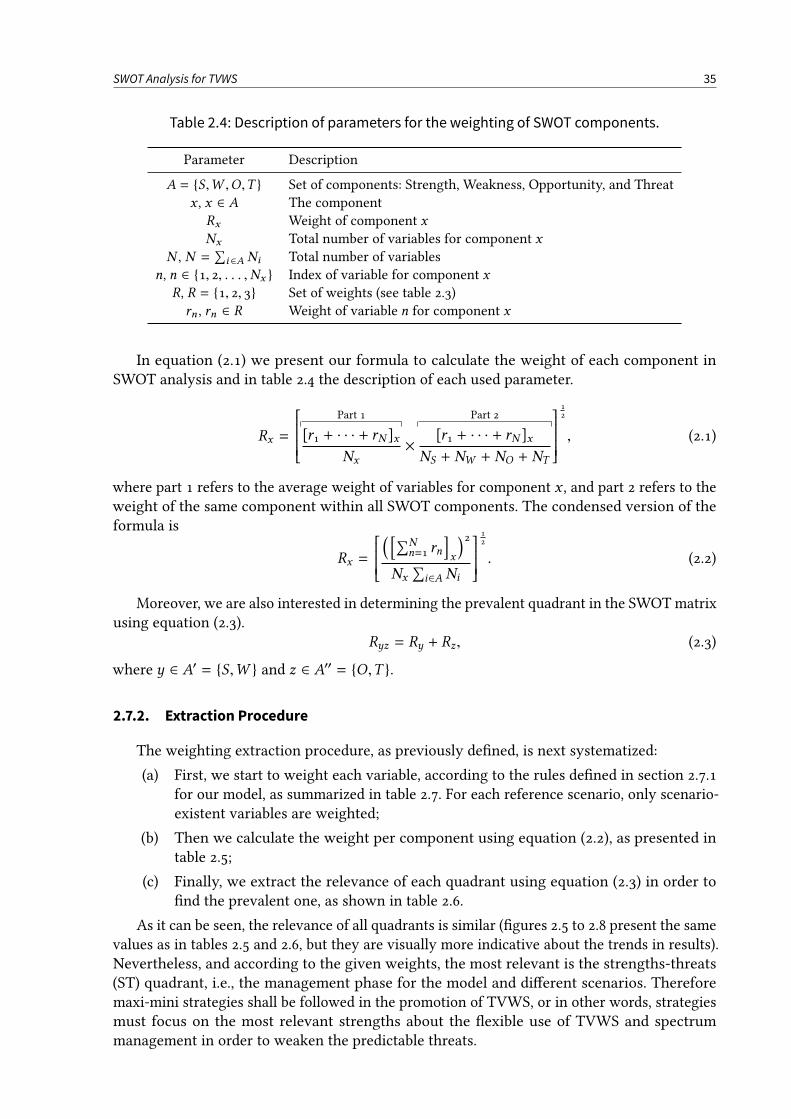
SWOT Analysis for TVWS 35
Table 2.4: Description of parameters for the weighting of SWOT components.
Parameter Description
A = S,W ,O,T Set of components: Strength, Weakness, Opportunity, and Threatx , x ∈ A The component
Rx Weight of component xNx Total number of variables for component x
N , N =∑
i ∈A Ni Total number of variablesn, n ∈ 1, 2, . . . ,Nx Index of variable for component x
R, R = 1, 2, 3 Set of weights (see table 2.3)rn , rn ∈ R Weight of variable n for component x
In equation (2.1) we present our formula to calculate the weight of each component inSWOT analysis and in table 2.4 the description of each used parameter.
Rx =
Part 1
[r1 + · · · + rN ]xNx
×
Part 2
[r1 + · · · + rN ]xNS + NW + NO + NT
12
, (2.1)
where part 1 refers to the average weight of variables for component x , and part 2 refers to theweight of the same component within all SWOT components. The condensed version of theformula is
Rx =
( [∑Nn=1 rn
]x
)2
Nx∑
i∈A Ni
12
. (2.2)
Moreover, we are also interested in determining the prevalent quadrant in the SWOTmatrixusing equation (2.3).
Ryz = Ry + Rz, (2.3)
where y ∈ A′ = S,W and z ∈ A′′ = O,T .
2.7.2. Extraction Procedure
The weighting extraction procedure, as previously dened, is next systematized:
(a) First, we start to weight each variable, according to the rules dened in section 2.7.1for our model, as summarized in table 2.7. For each reference scenario, only scenario-existent variables are weighted;
(b) Then we calculate the weight per component using equation (2.2), as presented intable 2.5;
(c) Finally, we extract the relevance of each quadrant using equation (2.3) in order tond the prevalent one, as shown in table 2.6.
As it can be seen, the relevance of all quadrants is similar (gures 2.5 to 2.8 present the samevalues as in tables 2.5 and 2.6, but they are visually more indicative about the trends in results).Nevertheless, and according to the given weights, the most relevant is the strengths-threats(ST) quadrant, i.e., the management phase for the model and dierent scenarios. Thereforemaxi-mini strategies shall be followed in the promotion of TVWS, or in other words, strategiesmust focus on the most relevant strengths about the exible use of TVWS and spectrummanagement in order to weaken the predictable threats.
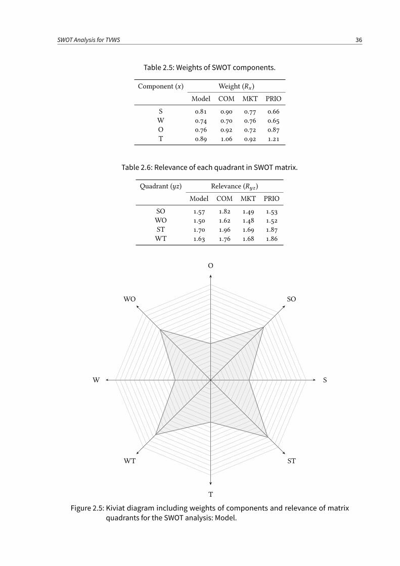
SWOT Analysis for TVWS 36
Table 2.5: Weights of SWOT components.
Component (x ) Weight (Rx )
Model COM MKT PRIO
S 0.81 0.90 0.77 0.66W 0.74 0.70 0.76 0.65O 0.76 0.92 0.72 0.87T 0.89 1.06 0.92 1.21
Table 2.6: Relevance of each quadrant in SWOTmatrix.
Quadrant (yz) Relevance (Ryz )
Model COM MKT PRIO
SO 1.57 1.82 1.49 1.53WO 1.50 1.62 1.48 1.52ST 1.70 1.96 1.69 1.87WT 1.63 1.76 1.68 1.86
S
SO
O
WO
W
WT
T
ST
Figure 2.5: Kiviat diagram including weights of components and relevance of matrix
quadrants for the SWOT analysis: Model.
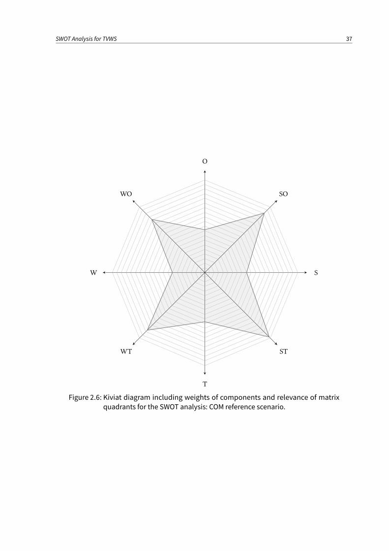
SWOT Analysis for TVWS 37
S
SO
O
WO
W
WT
T
ST
Figure 2.6: Kiviat diagram including weights of components and relevance of matrix
quadrants for the SWOT analysis: COM reference scenario.
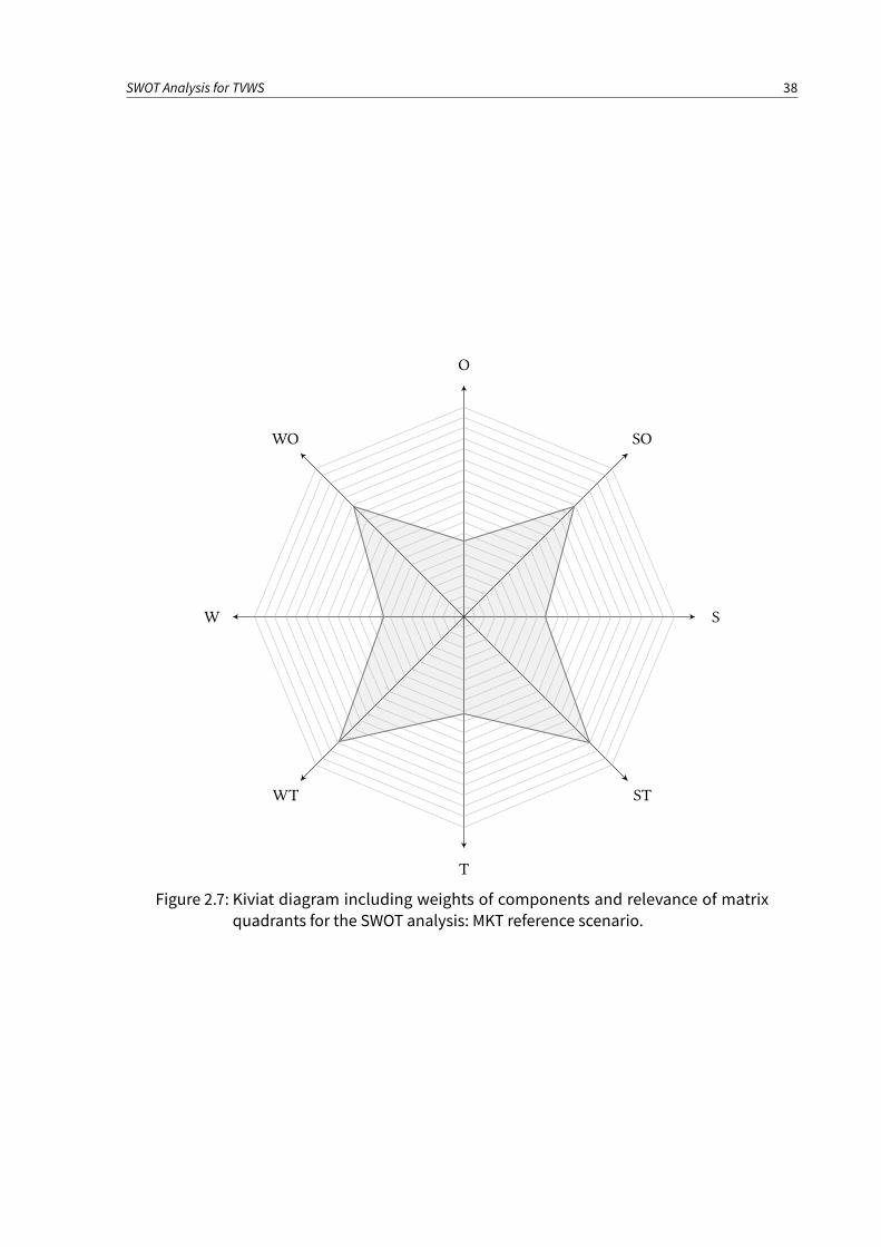
SWOT Analysis for TVWS 38
S
SO
O
WO
W
WT
T
ST
Figure 2.7: Kiviat diagram including weights of components and relevance of matrix
quadrants for the SWOT analysis: MKT reference scenario.
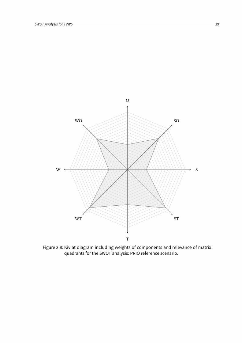
SWOT Analysis for TVWS 39
S
SO
O
WO
W
WT
T
ST
Figure 2.8: Kiviat diagram including weights of components and relevance of matrix
quadrants for the SWOT analysis: PRIO reference scenario.
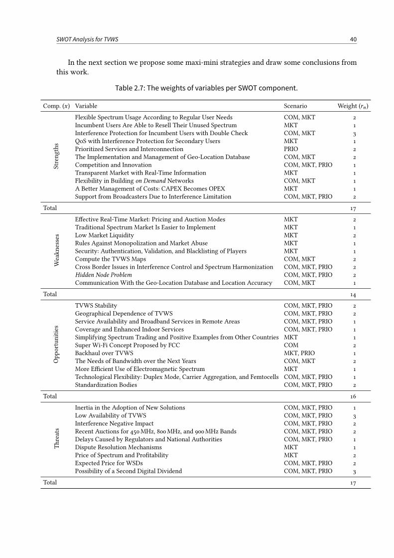
SWOT Analysis for TVWS 40
In the next section we propose some maxi-mini strategies and draw some conclusions fromthis work.
Table 2.7: The weights of variables per SWOT component.
Comp. (x ) Variable Scenario Weight (rn )
Strengths
Flexible Spectrum Usage According to Regular User Needs COM, MKT 2Incumbent Users Are Able to Resell Their Unused Spectrum MKT 1Interference Protection for Incumbent Users with Double Check COM, MKT 3QoS with Interference Protection for Secondary Users MKT 1Prioritized Services and Interconnection PRIO 2The Implementation and Management of Geo-Location Database COM, MKT 2Competition and Innovation COM, MKT, PRIO 1Transparent Market with Real-Time Information MKT 1Flexibility in Building on Demand Networks COM, MKT 1A Better Management of Costs: CAPEX Becomes OPEX MKT 1Support from Broadcasters Due to Interference Limitation COM, MKT, PRIO 2
Total 17
Weakn
esses
Eective Real-Time Market: Pricing and Auction Modes MKT 2Traditional Spectrum Market Is Easier to Implement MKT 1Low Market Liquidity MKT 2Rules Against Monopolization and Market Abuse MKT 1Security: Authentication, Validation, and Blacklisting of Players MKT 1Compute the TVWS Maps COM, MKT 2Cross Border Issues in Interference Control and Spectrum Harmonization COM, MKT, PRIO 2Hidden Node Problem COM, MKT, PRIO 2Communication With the Geo-Location Database and Location Accuracy COM, MKT 1
Total 14
Opp
ortunities
TVWS Stability COM, MKT, PRIO 2Geographical Dependence of TVWS COM, MKT, PRIO 2Service Availability and Broadband Services in Remote Areas COM, MKT, PRIO 1Coverage and Enhanced Indoor Services COM, MKT, PRIO 1Simplifying Spectrum Trading and Positive Examples from Other Countries MKT 1Super Wi-Fi Concept Proposed by FCC COM 2Backhaul over TVWS MKT, PRIO 1The Needs of Bandwidth over the Next Years COM, MKT 2More Ecient Use of Electromagnetic Spectrum MKT 1Technological Flexibility: Duplex Mode, Carrier Aggregation, and Femtocells COM, MKT, PRIO 1Standardization Bodies COM, MKT, PRIO 2
Total 16
Threats
Inertia in the Adoption of New Solutions COM, MKT, PRIO 1Low Availability of TVWS COM, MKT, PRIO 3Interference Negative Impact COM, MKT, PRIO 2Recent Auctions for 450MHz, 800MHz, and 900MHz Bands COM, MKT, PRIO 2Delays Caused by Regulators and National Authorities COM, MKT, PRIO 1Dispute Resolution Mechanisms MKT 1Price of Spectrum and Protability MKT 2Expected Price for WSDs COM, MKT, PRIO 2Possibility of a Second Digital Dividend COM, MKT, PRIO 3
Total 17
SWOT Analysis for TVWS 41
2.8. Conclusions
In this chapter we presented a suitable SWOT analysis for the use of TVWS in threereference scenarios mainly considering the European context. The analysis provided herein isvery exible, since with few changes it can be applied to dierent scenarios in the use of TVWSor other contexts/markets. For example, the analysis was performed for the model and each ofthe reference scenarios, but it could be done considering the combination of two scenarios. Assuch, it would be necessary to select the common variables within the scenarios under studyand repeat the whole process explained in section 2.7.
In the present study, the most relevant quadrant is the strengths-threats (ST) or themanagement phase. This happens mainly because most of the important threats to our modelare related with the absence of TVWS as the whole model relies on them, mainly because:(a) TVWS will not exist if they become part of the traditional market; (b) And TVWS are onlyavailable because incumbents, namely broadcasters, are not using them.
Regulators, TV broadcasters, and mobile operators are accustomed to a traditional spectrummarket, where only strongly positioned players are able to go for auctions and where theleased rights are for long periods of time. Moreover, as common sense, in traditional spectrummarkets, players are in the safe place because they are protected from harmful interference.
Therefore, the TVWS defenders shall focus on the promotion of a real-time secondaryspectrum market, where through the correct implementation of policies for protection ratiosand with the safe harbor concept, incumbents are protected against interference.
Also important is to stimulate the development of innovative business models such thatimportant TV stakeholders, like broadcasters and mobile operators will make part of a valuablechain, thus encouraging regulators to develop supportive policies for the functioning ofsecondary spectrum markets.
Moreover, our model promotes the spectrum democratization, either with or without QoSguarantees, where all players can aord it. Furthermore, new business opportunities likemanaging the broker or the geo-location database may be real. All of this would make thespectrum business even more protable.
Finally, SWOT analysis is prone to suer from subjective bias [98] and as such shouldbe complemented by other strategic analysis tools like, for instance, the Porter’s Five Forcesmodel [99], [100] or Analytic Hierarchy Process (AHP) [101] that can conrm its conclusions.
CHAPTER 3
Techno-Economic Evaluation for TVWS
E valuating the deployment of a Long Term Evolution (LTE) network over Television WhiteSpaces (TVWS) (700MHz) against the legacy (2.60GHz) carrier frequencies in terms of
costs, Capital Expenditure (CAPEX) and Operational Expenditure (OPEX), and the Net PresentValue (NPV) gure, is essential to convince operators to support/adopt a more exible spectrummarket approach. The evaluation performed in this chapter is done for a period of ve yearsand considers as an example the city of Munich in Germany and its metropolitan area; formallya square of 50 × 50 km. Moreover, three dierent network deployment scenarios are taken intoconsideration: only with the 2.60GHz legacy carrier (scenario 1), only with the 700MHz TVWScarrier (scenario 2), and using the legacy carrier plus an additional TVWS carrier (scenario 3).The sensitivity analysis (NPV variance or protability) to the change of input parametersin those three dierent network deployments is also done. Those changes are related withclients base, price of devices and device subsidies, Average Return Per User (ARPU), opticalber infrastructure, cost of spectrum in traditional and secondary markets, and average use ofTVWS. Results show that while being more protable to buy spectrum in traditional marketand follow the deployment scenario 2, the combination of legacy carrier and TVWS carrier(acquired through the secondary spectrum market), i.e., deployment scenario 3, closely followsthe best result. Moreover, the protability is very sensitive to ARPU and less sensitive to, e.g.,price of devices or spectrum.
3.1. Methodology for Network Techno-Economic Evaluation
The economic metric used for techno-economic evaluation is the NPV since it is one of themost widely used and reliable indicators to evaluate the feasibility of a project. Hence, in orderto compute the NPV we must clearly understand what are the revenues and costs. The scenariowe consider is of a single operator (in which there is no renting income). In this case, revenuesare only the sum of all payments done by clients considering the services they have contracted.
The costs of building and running a broadband network can be divided into CAPEXand OPEX. CAPEX includes the investments in the network infrastructure and devices, aswell as the hardware required for Operational & Maintenance (O&M) functions, such asnetworkmanagement and billing/charging systems. OPEX includes the labor costs and expensesoriginated from running and managing the network as well as costs related to, for example,marketing, sales, and clients care.
As an example, consider that we want to buy a new car. The CAPEX is, e.g., the moneypayed to the seller, either paid all at once or by paying a xed amount per month, plus themoney to buy a garage to park the car. On the other hand, OPEX can be considered as themoney in renting the garage, to pay for the general maintenance and car repair, plus the moneyspent for lling the car tank with fuel and replacing the wheels.
42
Techno-Economic Evaluation for TVWS 43
The OPEX related with a certain project is often more dicult to predict than the CAPEX.This is especially true when new technologies are considered, as the previous experience and/ordata are not available.
When revenues, investments, and all operational costs are estimated for each year of theperiod under study (N years), the cash ow CF(n), n ∈ 0, 1, ...,N , can be established
CF(n) = Revenues(n) − CAPEX(n) − OPEX(n). (3.1)
The time-value of money and risks are taken into account in the discount rate r (sometimesalso referred as interest rate). Therefore, the discounted cash ow is dened as
DCF(n) =CF(n)
(1 + r )n. (3.2)
Finally, the sum of all discounted cash ows is known as the NPV,
NPV = CF(0) +N∑
n=1
DCF(n) =N∑
n=0
DCF(n). (3.3)
The NPV1 is a measure of the value of a project. Putting it simply, if NPV is positive theinvestment adds value to the company and the project is protable; while for the opposite, i.e.,if NPV is negative, the investment subtracts value from the company and the project shall beabandoned or reformulated; nally, if NPV equals zero then the investment neither gains norloses value for the company, thus in this case the nal decision shall be based on other criteria,e.g., strategic position. In [103] the decision criteria is further explained based on the analysisof project risks.
Hence, the NPV rule states that a company should invest in any project with a positive NPV,and since it incorporates the discount rate, it represents the expected return that is forgone byinvesting in the project rather than in comparable nancial securities. Other methods, such asInternal Rate of Return (IRR) rule or the payback rule, also used in protability assessment,have some pitfalls and deciencies [104] when compared with the NPV method, and thereforeare not used.
Additionally, the rst year or year of implementation (y0) is mainly dealt with investments.As such, the CF(0) is expected to be negative; for educational purposes, CF(0) is commonlyplaced to the left of the sum to emphasize its role as (minus) the investment.
3.1.1. Scenario Description
For a comparative study on expenditures of deploying and operating a LTE network overTVWS (700MHz) against the legacy (2.60GHz) carrier frequencies, it is required the knowledgeabout the scenario where the LTE network will be deployed. In this context, we present thecharacterization of the area under study in terms of occupied area, population density, clientsbase, and number of active users. Also, we consider a LTE network with its main entities, andalso a spectrum broker and the geo-location database.
1 For more information about the historical use of NPV, see [102].
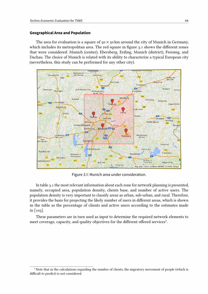
Techno-Economic Evaluation for TVWS 44
Geographical Area and Population
The area for evaluation is a square of 50 × 50 km around the city of Munich in Germany,which includes its metropolitan area. The red square in gure 3.1 shows the dierent zonesthat were considered: Munich (center), Ebersberg, Erding, Munich (district), Freising, andDachau. The choice of Munich is related with its ability to characterize a typical European city(nevertheless, this study can be performed for any other city).
Figure 3.1: Munich area under consideration.
In table 3.1 the most relevant information about each zone for network planning is presented,namely, occupied area, population density, clients base, and number of active users. Thepopulation density is very important to classify areas as urban, sub-urban, and rural. Therefore,it provides the basis for projecting the likely number of users in dierent areas, which is shownin the table as the percentage of clients and active users according to the estimates madein [105].
These parameters are in turn used as input to determine the required network elements tomeet coverage, capacity, and quality objectives for the dierent oered services2.
2 Note that in the calculations regarding the number of clients, the migratory movement of people (which isdicult to predict) is not considered.
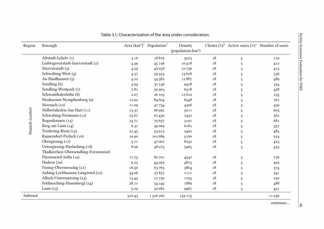
Techno-EconomicEvaluationforTVWS
45
Table 3.1: Characterization of the area under consideration.
Region Borough Area (km2)† Population† Density(population/km2)
Clients (%)‡ Active users (%)∗ Number of users
Altstadt-Lehelv (1) 3.16 18 876 5973 18 5 170Ludwigsvorstadt-Isarvorstadt (2) 4.39 45 736 10 418 18 5 412Maxvorstadt (3) 4.29 46 058 10 736 18 5 415Schwabing-West (4) 4.37 59 553 13 628 18 5 536Au-Haidhausen (5) 4.22 54 382 12 887 18 5 489Sendling (6) 3.94 37 146 9428 18 5 334Sendling-Westpark (7) 7.81 50 903 6518 18 5 458Schwanthalerhöhe (8) 2.07 26 103 12 610 18 5 235Neuhausen-Nymphenburg (9) 12.92 84 604 6548 18 5 761Moosach (10) 11.09 47 754 4306 18 5 430Milbertshofen-Am Hart (11) 13.37 66 992 5011 18 5 603Schwabing-Freimann (12) 25.67 62 430 2432 18 5 562Bogenhausen (13) 23.71 75 657 3191 18 5 681Berg am Laim (14) 6.31 39 009 6182 18 5 351Trudering-Riem (15) 22.45 53 915 2402 18 5 485Ramersdorf-Perlach (16) 19.90 102 689 5160 18 5 924Obergiesing (17) 5.71 47 007 8232 18 5 423Untergiesing-Harlaching (18) 8.06 48 075 5965 18 5 433Thalkirchen-Obersendling-Forstenried-Fürstenried-Solln (19) 17.75 80 701 4547 18 5 726Hadern (20) 9.23 44 993 4875 18 5 405Pasing-Obermenzing (21) 16.50 63 763 3864 18 5 574Aubing-Lochhausen-Langwied (22) 34.06 37 857 1111 18 5 341Allach-Untermenzing (23) 15.45 27 730 1795 18 5 250Feldmoching-Hasenbergl (24) 28.71 54 245 1889 18 5 488
Munich(center)
Laim (25) 5.29 50 082 9467 18 5 451
Subtotal 310.43 1 326 260 159 175 11 936
continues. . .
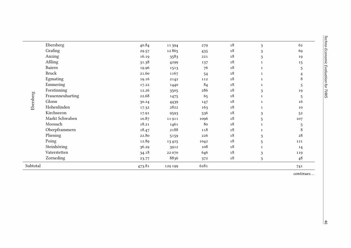
Techno-EconomicEvaluationforTVWS
46
Ebersberg 40.84 11 394 279 18 3 62Grang 29.57 12 865 435 18 3 69Anzing 16.19 3583 221 18 3 19Aßling 31.38 4299 137 18 1 15Baiern 19.96 1513 76 18 1 5Bruck 21.60 1167 54 18 1 4Egmating 19.16 2142 112 18 1 8Emmering 17.22 1440 84 18 1 5Forstinning 12.26 3505 286 18 3 19Frauenneuharting 22.68 1475 65 18 1 5Glonn 30.24 4439 147 18 1 16Hohenlinden 17.32 2822 163 18 1 10Kirchseeon 17.91 9593 536 18 3 52Markt Schwaben 10.87 11 911 1096 18 5 107Moosach 18.21 1461 80 18 1 5Oberpframmern 18.47 2188 118 18 1 8Pliening 22.80 5159 226 18 3 28Poing 12.89 13 425 1042 18 5 121Steinhöring 36.29 3912 108 18 1 14Vaterstetten 34.18 22 070 646 18 3 119
Ebersberg
Zorneding 23.77 8836 372 18 3 48
Subtotal 473.81 129 199 6281 741
continues. . .
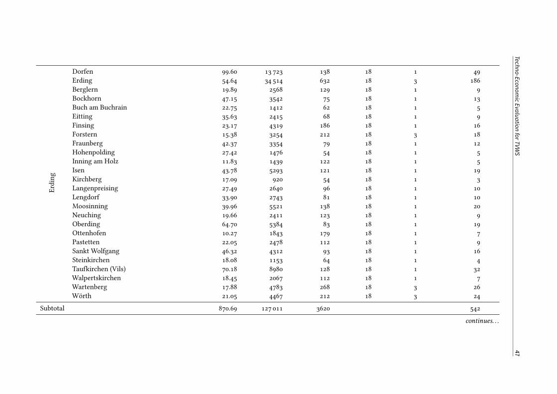
Techno-EconomicEvaluationforTVWS
47
Dorfen 99.60 13 723 138 18 1 49Erding 54.64 34 514 632 18 3 186Berglern 19.89 2568 129 18 1 9Bockhorn 47.15 3542 75 18 1 13Buch am Buchrain 22.75 1412 62 18 1 5Eitting 35.63 2415 68 18 1 9Finsing 23.17 4319 186 18 1 16Forstern 15.38 3254 212 18 3 18Fraunberg 42.37 3354 79 18 1 12Hohenpolding 27.42 1476 54 18 1 5Inning am Holz 11.83 1439 122 18 1 5Isen 43.78 5293 121 18 1 19Kirchberg 17.09 920 54 18 1 3Langenpreising 27.49 2640 96 18 1 10Lengdorf 33.90 2743 81 18 1 10Moosinning 39.96 5521 138 18 1 20Neuching 19.66 2411 123 18 1 9Oberding 64.70 5384 83 18 1 19Ottenhofen 10.27 1843 179 18 1 7Pastetten 22.05 2478 112 18 1 9Sankt Wolfgang 46.32 4312 93 18 1 16Steinkirchen 18.08 1153 64 18 1 4Taufkirchen (Vils) 70.18 8980 128 18 1 32Walpertskirchen 18.45 2067 112 18 1 7Wartenberg 17.88 4783 268 18 3 26
Erding
Wörth 21.05 4467 212 18 3 24
Subtotal 870.69 127 011 3620 542
continues. . .
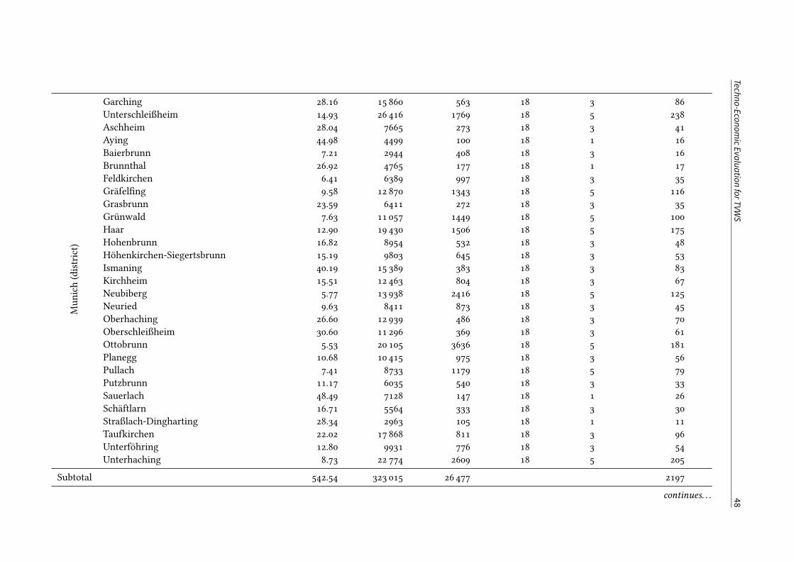
Techno-EconomicEvaluationforTVWS
48
Garching 28.16 15 860 563 18 3 86Unterschleißheim 14.93 26 416 1769 18 5 238Aschheim 28.04 7665 273 18 3 41Aying 44.98 4499 100 18 1 16Baierbrunn 7.21 2944 408 18 3 16Brunnthal 26.92 4765 177 18 1 17Feldkirchen 6.41 6389 997 18 3 35Gräfelng 9.58 12 870 1343 18 5 116Grasbrunn 23.59 6411 272 18 3 35Grünwald 7.63 11 057 1449 18 5 100Haar 12.90 19 430 1506 18 5 175Hohenbrunn 16.82 8954 532 18 3 48Höhenkirchen-Siegertsbrunn 15.19 9803 645 18 3 53Ismaning 40.19 15 389 383 18 3 83Kirchheim 15.51 12 463 804 18 3 67Neubiberg 5.77 13 938 2416 18 5 125Neuried 9.63 8411 873 18 3 45Oberhaching 26.60 12 939 486 18 3 70Oberschleißheim 30.60 11 296 369 18 3 61Ottobrunn 5.53 20 105 3636 18 5 181Planegg 10.68 10 415 975 18 3 56Pullach 7.41 8733 1179 18 5 79Putzbrunn 11.17 6035 540 18 3 33Sauerlach 48.49 7128 147 18 1 26Schäftlarn 16.71 5564 333 18 3 30Straßlach-Dingharting 28.34 2963 105 18 1 11Taufkirchen 22.02 17 868 811 18 3 96Unterföhring 12.80 9931 776 18 3 54
Munich(district)
Unterhaching 8.73 22 774 2609 18 5 205
Subtotal 542.54 323 015 26 477 2197
continues. . .
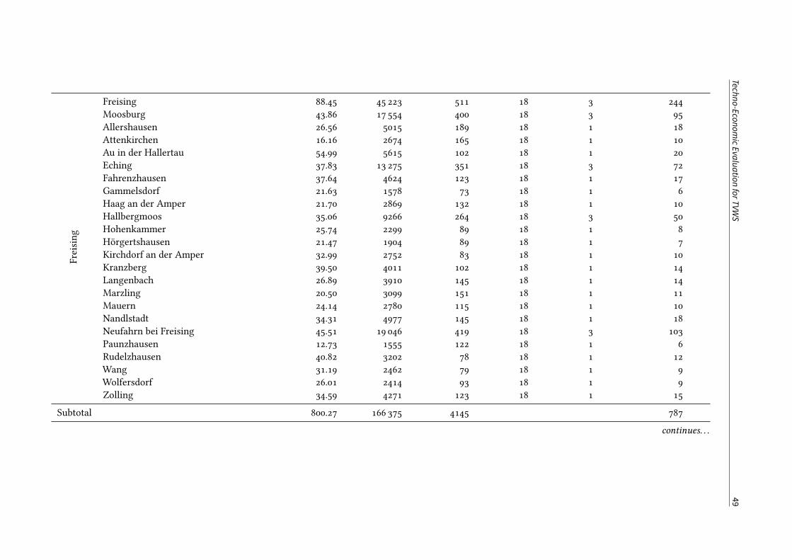
Techno-EconomicEvaluationforTVWS
49
Freising 88.45 45 223 511 18 3 244Moosburg 43.86 17 554 400 18 3 95Allershausen 26.56 5015 189 18 1 18Attenkirchen 16.16 2674 165 18 1 10Au in der Hallertau 54.99 5615 102 18 1 20Eching 37.83 13 275 351 18 3 72Fahrenzhausen 37.64 4624 123 18 1 17Gammelsdorf 21.63 1578 73 18 1 6Haag an der Amper 21.70 2869 132 18 1 10Hallbergmoos 35.06 9266 264 18 3 50Hohenkammer 25.74 2299 89 18 1 8Hörgertshausen 21.47 1904 89 18 1 7Kirchdorf an der Amper 32.99 2752 83 18 1 10Kranzberg 39.50 4011 102 18 1 14Langenbach 26.89 3910 145 18 1 14Marzling 20.50 3099 151 18 1 11Mauern 24.14 2780 115 18 1 10Nandlstadt 34.31 4977 145 18 1 18Neufahrn bei Freising 45.51 19 046 419 18 3 103Paunzhausen 12.73 1555 122 18 1 6Rudelzhausen 40.82 3202 78 18 1 12Wang 31.19 2462 79 18 1 9Wolfersdorf 26.01 2414 93 18 1 9
Freising
Zolling 34.59 4271 123 18 1 15
Subtotal 800.27 166 375 4145 787
continues. . .
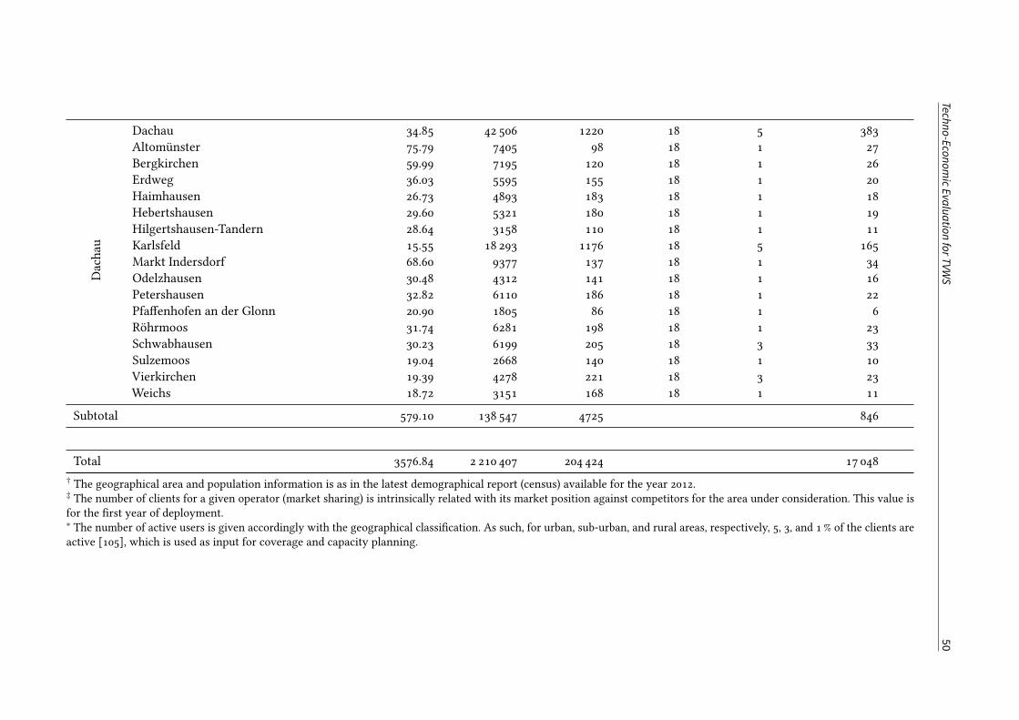
Techno-EconomicEvaluationforTVWS
50
Dachau 34.85 42 506 1220 18 5 383Altomünster 75.79 7405 98 18 1 27Bergkirchen 59.99 7195 120 18 1 26Erdweg 36.03 5595 155 18 1 20Haimhausen 26.73 4893 183 18 1 18Hebertshausen 29.60 5321 180 18 1 19Hilgertshausen-Tandern 28.64 3158 110 18 1 11Karlsfeld 15.55 18 293 1176 18 5 165Markt Indersdorf 68.60 9377 137 18 1 34Odelzhausen 30.48 4312 141 18 1 16Petershausen 32.82 6110 186 18 1 22Pfaenhofen an der Glonn 20.90 1805 86 18 1 6Röhrmoos 31.74 6281 198 18 1 23Schwabhausen 30.23 6199 205 18 3 33Sulzemoos 19.04 2668 140 18 1 10Vierkirchen 19.39 4278 221 18 3 23
Dachau
Weichs 18.72 3151 168 18 1 11
Subtotal 579.10 138 547 4725 846
Total 3576.84 2 210 407 204 424 17 048
† The geographical area and population information is as in the latest demographical report (census) available for the year 2012.‡ The number of clients for a given operator (market sharing) is intrinsically related with its market position against competitors for the area under consideration. This value isfor the rst year of deployment.∗ The number of active users is given accordingly with the geographical classication. As such, for urban, sub-urban, and rural areas, respectively, 5, 3, and 1 % of the clients areactive [105], which is used as input for coverage and capacity planning.
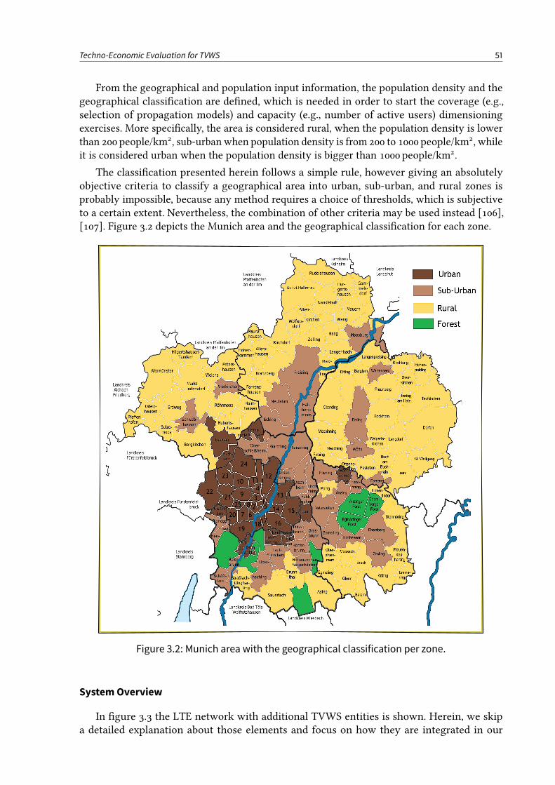
Techno-Economic Evaluation for TVWS 51
From the geographical and population input information, the population density and thegeographical classication are dened, which is needed in order to start the coverage (e.g.,selection of propagation models) and capacity (e.g., number of active users) dimensioningexercises. More specically, the area is considered rural, when the population density is lowerthan 200 people/km2, sub-urban when population density is from 200 to 1000 people/km2, whileit is considered urban when the population density is bigger than 1000 people/km2.
The classication presented herein follows a simple rule, however giving an absolutelyobjective criteria to classify a geographical area into urban, sub-urban, and rural zones isprobably impossible, because any method requires a choice of thresholds, which is subjectiveto a certain extent. Nevertheless, the combination of other criteria may be used instead [106],[107]. Figure 3.2 depicts the Munich area and the geographical classication for each zone.
Figure 3.2: Munich area with the geographical classification per zone.
SystemOverview
In gure 3.3 the LTE network with additional TVWS entities is shown. Herein, we skipa detailed explanation about those elements and focus on how they are integrated in our
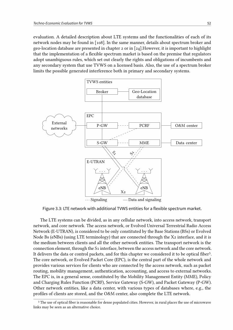
Techno-Economic Evaluation for TVWS 52
evaluation. A detailed description about LTE systems and the functionalities of each of itsnetwork nodes may be found in [108]. In the same manner, details about spectrum broker andgeo-location database are presented in chapter 2 or in [24].However, it is important to highlightthat the implementation of a exible spectrum market is based on the premise that regulatorsadopt unambiguous rules, which set out clearly the rights and obligations of incumbents andany secondary system that use TVWS on a licensed basis. Also, the use of a spectrum brokerlimits the possible generated interference both in primary and secondary systems.
Broker Geo-Location
database
P-GW PCRF
S-GW MME
EPC
E-UTRAN
TVWS entities
External
networksO&M center
Data center
X2
S1
S1
eNB
. . .
eNB
. . .
Signaling Data and signaling
Figure 3.3: LTE network with additional TVWS entities for a flexible spectrummarket.
The LTE systems can be divided, as in any cellular network, into access network, transportnetwork, and core network. The access network, or Evolved Universal Terrestrial Radio AccessNetwork (E-UTRAN), is considered to be only constituted by the Base Stations (BSs) or EvolvedNode Bs (eNBs) (using LTE terminology) that are connected through the X2 interface, and it isthe medium between clients and all the other network entities. The transport network is theconnection element, through the S1 interface, between the access network and the core network.It delivers the data or control packets, and for this chapter we considered it to be optical ber3.The core network, or Evolved Packet Core (EPC), is the central part of the whole network andprovides various services for clients who are connected by the access network, such as packetrouting, mobility management, authentication, accounting, and access to external networks.The EPC is, in a general sense, constituted by the Mobility Management Entity (MME), Policyand Charging Rules Function (PCRF), Service Gateway (S-GW), and Packet Gateway (P-GW).Other network entities, like a data center, with various types of databases where, e.g., theproles of clients are stored, and the O&M center, also complete the LTE network.
3 The use of optical ber is reasonable for dense populated cities. However, in rural places the use of microwavelinks may be seen as an alternative choice.
Techno-Economic Evaluation for TVWS 53
The EPC may be limited by two factors: rst, the number of BSs that can be connected to asingle MME; second, the amount of trac that can be processed at the same time by the S-GWand P-GW. It is assumed that if a new pair of S-GW and P-GW is required, then a new EPCis required. However, in many cases, a new MME is not required because it only processescontrol information and can handle a large amount of connected BSs.
Moreover, the BSs are connected to each other through the X2 interface, which mostlycarries control information, andmay be seen as a logical link. Practically speaking, and assumingthe delay in the transport network can be neglected, the X2 interface can be implementedthrough the core network and multiplexed in only one optical ber. Therefore, from each BS tothe core network we only assume one optical ber link, which has enough capacity to deliverall the trac that comes and goes from the BS to the core network and vice-versa.
Finally, the costs associated with the broker and geo-location database (either investmentsor running costs) are not considered. However, if they were considered and since the numberof such elements do not scale with the network size, their impact would be the same in all threedierent network deployments, and for comparative studies the related gains/losses would notchange.
3.2. Network Infrastructure
The network planning is performed to determine the number of BSs that are needed (bothin terms of coverage and capacity) to serve a certain region (i.e., satisfy users’ throughputdemands). The number of BSs has a direct inuence on the costs for operators because, apartfrom the direct costs associated with BSs (equipment, antennas, renting sites, cooling systems,etc.), it is also used to calculate the length of optical ber infrastructure to connect the accessand core networks. Moreover, the EPC is also limited by the number of connected BSs.
Herein, we are also interested in reducing the implementation and operational costs whilemaintaining the network performance, which may be achieved with the introduction of TVWS,because expectedly less BSs (thus less costs) are required for the same area; or with someincrease in network costs, more capacity can be delivered.
Therefore, a radio network dimensioning tool for the area under consideration was em-ployed. In [105] the planning process both in terms of coverage and capacity is detailed described:a at network conguration, the percentage of clients and active users per geographical area,throughput per user, cell conguration, block rate, and pathloss models are the parameterstaken into consideration; for consistence, further details are omitted herein, but may be easilyfound in the referred literature.
Hence, the radio network dimensioning aims basically to estimate the number of requiredBSs. The network dimensioning process is based on a uniform distribution of clients insideeach borough, at morphology, and a regular BS distribution.
The network planning activities, explained in the next paragraphs, are the following:
• Radio link budget;
• Coverage and capacity analysis;
• Required number of BSs.
Techno-Economic Evaluation for TVWS 54
3.2.1. Radio Link Budget
The radio link budget is an accounting of all the gains and losses in a transmission system.It looks at the elements that will determine the signal strength arriving at the receiver. Theradio link budget includes the following items:
• Transmitter power;
• Antenna gains (receiver and transmitter);
• Antenna feeder losses (receiver and transmitter);
• Pathloss;
• Required Signal to Interference-plus-Noise Ratio (SINR).
With these parameters the maximum allowable pathloss for the required SINR is calculated,which can generally be written as
L = TxPower + TxGain − TxLoss + RxGain − RxLoss − SINRRequired − RxNoise. (3.4)
Where:
• L is the total pathloss between the transmitter signal to the receiver (in dB);
• TxPower is the power transmitted by the transmitter antenna (in dBm);
• TxGain represents the gain of transmitter antenna related Equivalent Isotropically Radi-ated Power (EIRP) (in dBi);
• TxLoss represents the transmitter losses (in dB);
• RxGain represents the gain of receiver antenna related EIRP (in dBi);
• RxLoss represents the receiver losses (in dB);
• SINRRequired is the minimum required SINR for the signal to be received at the receiverwith the necessary quality/strength, which in LTE is closely related with Modulationand Coding Scheme (MCS) and service quality provisioning (in dB);
• RxNoise is the noise power at receiver antenna (in dBm).
3.2.2. Coverage and Capacity Analysis
As explained in [105], the coverage planning gives an estimation of resources neededto provide service in the deployment area with the given system parameters, without anycapacity concern. Therefore, it gives an assessment of the resources needed to cover the areaunder consideration so that the transmitters and receivers can communicate to each other. Thecoverage analysis fundamentally remains the most critical step in the design of any network.
Appropriate selection of propagation models is required for the coverage analysis andestimate the number of BSs needed to provide service in the deployment area. The cell radius ofa particular LTE sector is calculated through the maximum allowable loss (maximum allowablepathloss using equation (3.4) plus the shadowing margin) both in Downlink (DL) (BS-userdirection) and Uplink (UL) (user-BS direction) for the required SINR. Thereby, the maximumcoverage range of a cell is the minimum between DL and UL calculations, which are obtainedthrough the Erceg Extendedmodel [109], [110] for the deployment in 2.60GHz and the OkumuraHata model [111] for the deployment in 700MHz.
Techno-Economic Evaluation for TVWS 55
The Erceg Extended model distinguishes three terrain categories, called A, B, and C.Category A is for a terrain with the highest pathloss (hilly terrain with moderate-to-heavy treedensities) and is used for urban areas. Category B characterizes at terrains with intermediatepathloss condition or sub-urban areas. Category C is suitable for rural areas, where pathloss isthe lowest (mostly at terrain with light tree densities). Moreover, with appropriate frequencycorrection factors the model is “safely” used in the frequency range from 1 to 4GHz. In its turn,the Okumura Hata model, while comprising the same morphologies as the previous model, isused in the frequency range from 150 to 1500MHz. Thus, the propagation models are alignedwith the network deployment and geographical classication considered for this chapter.
Also the required SINR considers the kind of provided services. For that, we project that allactive users are served with a Constant Bit Rate (CBR) service of 1Mbps in DL and 256 kbps inUL. After achieving the number of BSs to cover the area under consideration, the next step isto analyze the capacity issue.
Each BS is limited in its capacity, i.e., there is a maximum amount of trac (throughput) thatit can handle. In some wireless cellular systems, like LTE, coverage and capacity are interrelated.In such cases, the main indicator of capacity is the SINR distribution over the cell, which isobtained by performing physical level simulations in a LTE simulator [105], [112], [113]. TheSINR distribution is directly mapped into system capacity, which is impacted by several factors,e.g., scheduler implementation, MCSs, antenna conguration/diversity, and interference levels.
As such, in order to map the inter-cell interference levels, dierent utilization factors pergeographical area (0.85 for urban, 0.88 for sub-urban, and 0.9 for rural) were used4 and themaximum throughput of a BS was calculated for the Single Input Single Output (SISO) antennaconguration, the system bandwidth of 5MHz [114] in each direction (DL and UL), consideringthe highest LTE MCS [115], and that each BS had three sectors.
The number of BSs regarding the capacity is then the ceiling calculation of the numberof users times the capacity of each user, divided by the capacity of each BS, divided by thenumber of sectors of each BS.
For network planning, the region under study was divided into boroughs and determinedthe number of BSs for each of them considering their population density. However, and mainlyin rural areas, it may happen that the number of calculated BSs is higher than the required one.This is true because with this approach, at least one BS is required per borough. Although, itcould happen that a neighbor BS had enough available capacity to accommodate more usersand, therefore, a BS becomes surplus.
3.2.3. Required Number of BSs
The coverage and the capacity planning are of essential importance in the whole radionetwork planning. The coverage planning determines the service range, while the capacityplanning determines the number of to-be-used BSs and their respective capacities. In this way,the main outcome of the network planning is the number of BSs to provide coverage and at thesame time fulll the projected quality objectives for the dierent oered services. Therefore,it is considered that the total number of BSs is calculated as the highest value between thecoverage and capacity calculations, as detailed in section 3.2.2.
As an example, table 3.2 shows the dierent number of calculated BSs for the legacy andTVWS bands in Munich (center) for the rst year. Clearly, the required number of BSs for
4 The inter-cell interference is predictably higher in urban areas than in sub-urban or rural areas.

Techno-Economic Evaluation for TVWS 56
frequency 2.60GHz is higher than in 700MHz, which in principle would bring advantages toreduce both CAPEX and OPEX.
Table 3.2: Number of BSs for 2.60 GHz and 700MHz in Munich (center) for the first year.
Region Borough Number of users† Number of BSs
2.60GHz 700MHz
Altstadt-Lehelv (1) 170 6 5Ludwigsvorstadt-Isarvorstadt (2) 412 14 12Maxvorstadt (3) 415 15 12Schwabing-West (4) 536 19 15Au-Haidhausen (5) 489 17 14Sendling (6) 334 12 10Sendling-Westpark (7) 458 16 13Schwanthalerhöhe (8) 235 8 7Neuhausen-Nymphenburg (9) 761 26 21Moosach (10) 430 15 12Milbertshofen-Am Hart (11) 603 21 17Schwabing-Freimann (12) 562 19 16Bogenhausen (13) 681 24 19Berg am Laim (14) 351 12 10Trudering-Riem (15) 485 17 14Ramersdorf-Perlach (16) 924 32 26Obergiesing (17) 423 15 12Untergiesing-Harlaching (18) 433 15 12Thalkirchen-Obersendling-Forstenried-Fürstenried-Solln (19) 726 25 20Hadern (20) 405 14 12Pasing-Obermenzing (21) 574 20 16Aubing-Lochhausen-Langwied (22) 341 12 10Allach-Untermenzing (23) 250 9 7Feldmoching-Hasenbergl (24) 488 17 14
Munich(center)
Laim (25) 451 16 13
Total 11 936 416 339
† The same information as in 8th column of table 3.1.
3.2.4. Core and Transport Network Dimensioning
In addition to the number of BSs, the network topology must also be considered. As it waspreviously mentioned, the interfaces X2/S1 (recall gure 3.3) are implemented through thecore network, and both data and control information may be multiplexed in the same opticallink. This is only true if the delay in the optical ber can be neglected (when compared to therequirements of most demanding services, e.g., real-time services) and there is enough capacityin a single ber to deliver all the trac from the BS that is connected to the core network,and vice-versa. In fact, the area under study is a small area of 50 × 50 km around a Europeanmetropolis, so the previous statement is expected to be true.
The total square area for evaluation may be divided into smaller squares. Each of thosesquares is named as EPC area and represents an area where all the BSs are connected to that
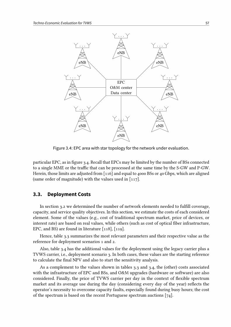
Techno-Economic Evaluation for TVWS 57
EPC
O&M center
Data center
eNB
. . .
eNB
. . .
eNB
. . .
eNB
. . .
eNB
. . .
eNB
. . .
eNB
. . .
eNB
. . .
Figure 3.4: EPC area with star topology for the network under evaluation.
particular EPC, as in gure 3.4. Recall that EPCs may be limited by the number of BSs connectedto a single MME or the trac that can be processed at the same time by the S-GW and P-GW.Herein, those limits are adjusted from [116] and equal to 4000 BSs or 40Gbps, which are aligned(same order of magnitude) with the values used in [117].
3.3. Deployment Costs
In section 3.2 we determined the number of network elements needed to fulll coverage,capacity, and service quality objectives. In this section, we estimate the costs of each consideredelement. Some of the values (e.g., cost of traditional spectrum market, price of devices, orinterest rate) are based on real values, while others (such as cost of optical ber infrastructure,EPC, and BS) are found in literature [118], [119].
Hence, table 3.3 summarizes the most relevant parameters and their respective value as thereference for deployment scenarios 1 and 2.
Also, table 3.4 has the additional values for the deployment using the legacy carrier plus aTVWS carrier, i.e., deployment scenario 3. In both cases, these values are the starting referenceto calculate the nal NPV and also to start the sensitivity analysis.
As a complement to the values shown in tables 3.3 and 3.4, the (other) costs associatedwith the infrastructure of EPC and BSs, and O&M upgrades (hardware or software) are alsoconsidered. Finally, the price of TVWS carrier per day in the context of exible spectrummarket and its average use during the day (considering every day of the year) reects theoperator’s necessity to overcome capacity faults, especially found during busy hours; the costof the spectrum is based on the recent Portuguese spectrum auctions [74].
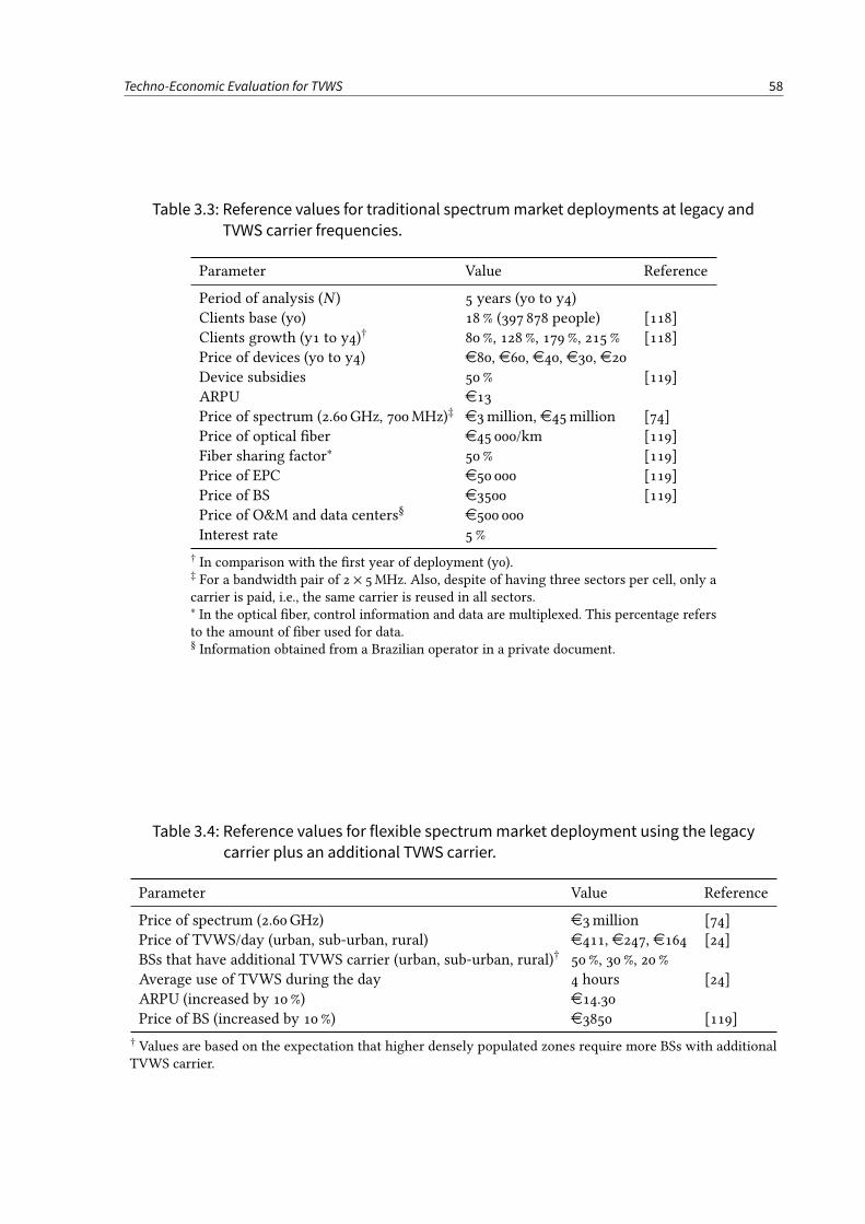
Techno-Economic Evaluation for TVWS 58
Table 3.3: Reference values for traditional spectrummarket deployments at legacy and
TVWS carrier frequencies.
Parameter Value Reference
Period of analysis (N ) 5 years (y0 to y4)Clients base (y0) 18 % (397 878 people) [118]Clients growth (y1 to y4)† 80 %, 128 %, 179 %, 215 % [118]Price of devices (y0 to y4) e80, e60, e40, e30, e20Device subsidies 50 % [119]ARPU e13Price of spectrum (2.60GHz, 700MHz)‡ e3million, e45million [74]Price of optical ber e45 000/km [119]Fiber sharing factor∗ 50 % [119]Price of EPC e50 000 [119]Price of BS e3500 [119]Price of O&M and data centers§ e500 000Interest rate 5 %
† In comparison with the rst year of deployment (y0).‡ For a bandwidth pair of 2 × 5MHz. Also, despite of having three sectors per cell, only acarrier is paid, i.e., the same carrier is reused in all sectors.∗ In the optical ber, control information and data are multiplexed. This percentage refersto the amount of ber used for data.§ Information obtained from a Brazilian operator in a private document.
Table 3.4: Reference values for flexible spectrummarket deployment using the legacy
carrier plus an additional TVWS carrier.
Parameter Value Reference
Price of spectrum (2.60GHz) e3million [74]Price of TVWS/day (urban, sub-urban, rural) e411, e247, e164 [24]BSs that have additional TVWS carrier (urban, sub-urban, rural)† 50 %, 30 %, 20 %Average use of TVWS during the day 4 hours [24]ARPU (increased by 10 %) e14.30Price of BS (increased by 10 %) e3850 [119]
† Values are based on the expectation that higher densely populated zones require more BSs with additionalTVWS carrier.
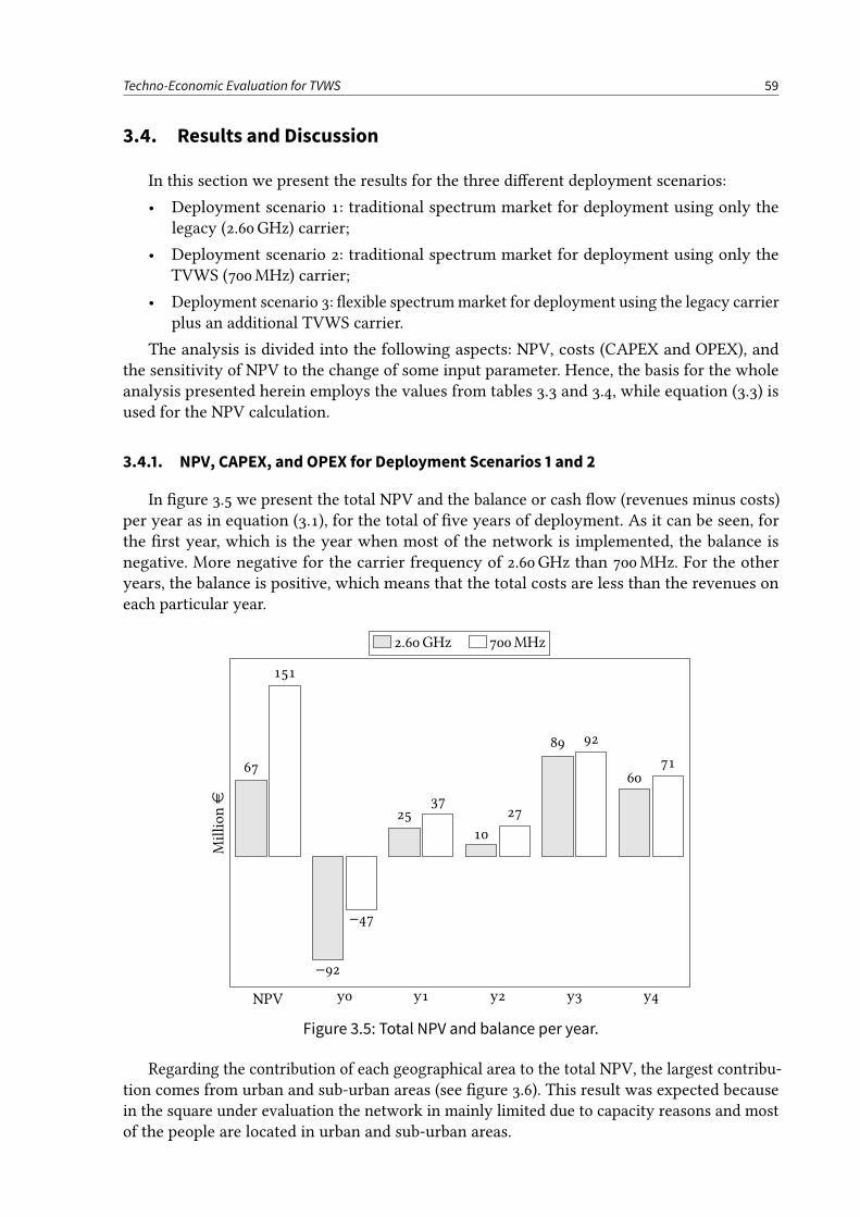
Techno-Economic Evaluation for TVWS 59
3.4. Results and Discussion
In this section we present the results for the three dierent deployment scenarios:
• Deployment scenario 1: traditional spectrum market for deployment using only thelegacy (2.60GHz) carrier;
• Deployment scenario 2: traditional spectrum market for deployment using only theTVWS (700MHz) carrier;
• Deployment scenario 3: exible spectrummarket for deployment using the legacy carrierplus an additional TVWS carrier.
The analysis is divided into the following aspects: NPV, costs (CAPEX and OPEX), andthe sensitivity of NPV to the change of some input parameter. Hence, the basis for the wholeanalysis presented herein employs the values from tables 3.3 and 3.4, while equation (3.3) isused for the NPV calculation.
3.4.1. NPV, CAPEX, and OPEX for Deployment Scenarios 1 and 2
In gure 3.5 we present the total NPV and the balance or cash ow (revenues minus costs)per year as in equation (3.1), for the total of ve years of deployment. As it can be seen, forthe rst year, which is the year when most of the network is implemented, the balance isnegative. More negative for the carrier frequency of 2.60GHz than 700MHz. For the otheryears, the balance is positive, which means that the total costs are less than the revenues oneach particular year.
NPV y0 y1 y2 y3 y4
67
−92
25
10
89
60
151
−47
3727
92
71
Millione
2.60GHz 700MHz
Figure 3.5: Total NPV and balance per year.
Regarding the contribution of each geographical area to the total NPV, the largest contribu-tion comes from urban and sub-urban areas (see gure 3.6). This result was expected becausein the square under evaluation the network in mainly limited due to capacity reasons and mostof the people are located in urban and sub-urban areas.
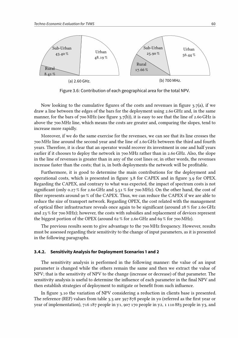
Techno-Economic Evaluation for TVWS 60
Urban
48.19 %
Sub-Urban
43.40 %
Rural
8.41 %
(a) 2.60 GHz.
Urban
56.44 %
Sub-Urban
25.90 %
Rural
17.66 %
(b) 700MHz.
Figure 3.6: Contribution of each geographical area for the total NPV.
Now looking to the cumulative gures of the costs and revenues in gure 3.7(a), if wedraw a line between the edges of the bars for the deployment using 2.60GHz and, in the samemanner, for the bars of 700MHz (see gure 3.7(b)), it is easy to see that the line of 2.60GHz isabove the 700MHz line, which means the costs are greater and, comparing the slopes, tend toincrease more rapidly.
Moreover, if we do the same exercise for the revenues, we can see that its line crosses the700MHz line around the second year and the line of 2.60GHz between the third and fourthyears. Therefore, it is clear that an operator would recover its investment in one and half yearsearlier if it chooses to deploy the network in 700MHz rather than in 2.60GHz. Also, the slopein the line of revenues is greater than in any of the cost lines or, in other words, the revenuesincrease faster than the costs; that is, in both deployments the network will be protable.
Furthermore, it is good to determine the main contributions for the deployment andoperational costs, which is presented in gure 3.8 for CAPEX and in gure 3.9 for OPEX.Regarding the CAPEX, and contrary to what was expected, the impact of spectrum costs is notsignicant (only 0.27 % for 2.60GHz and 5.51 % for 700MHz). On the other hand, the cost ofber represents around 90% of the CAPEX. Thus, we can reduce the CAPEX if we are able toreduce the size of transport network. Regarding OPEX, the cost related with the managementof optical ber infrastructure reveals once again to be signicant (around 28% for 2.60GHzand 23 % for 700MHz); however, the costs with subsidies and replacement of devices representthe biggest portion of the OPEX (around 62% for 2.60GHz and 69% for 700MHz).
The previous results seem to give advantage to the 700MHz frequency. However, resultsmust be assessed regarding their sensitivity to the change of input parameters, as it is presentedin the following paragraphs.
3.4.2. Sensitivity Analysis for Deployment Scenarios 1 and 2
The sensitivity analysis is performed in the following manner: the value of an inputparameter is changed while the others remain the same and then we extract the value ofNPV; that is the sensitivity of NPV to the change (increase or decrease) of that parameter. Thesensitivity analysis is useful to determine the inuence of each parameter in the nal NPV andthen establish strategies of deployment to mitigate or benet from such inuence.
In gure 3.10 the variation of NPV considering a reduction in clients base is presented.The reference (REF) values from table 3.3 are 397 878 people in y0 (referred as the rst year oryear of implementation), 716 187 people in y1, 907 170 people in y2, 1 110 883 people in y3, and
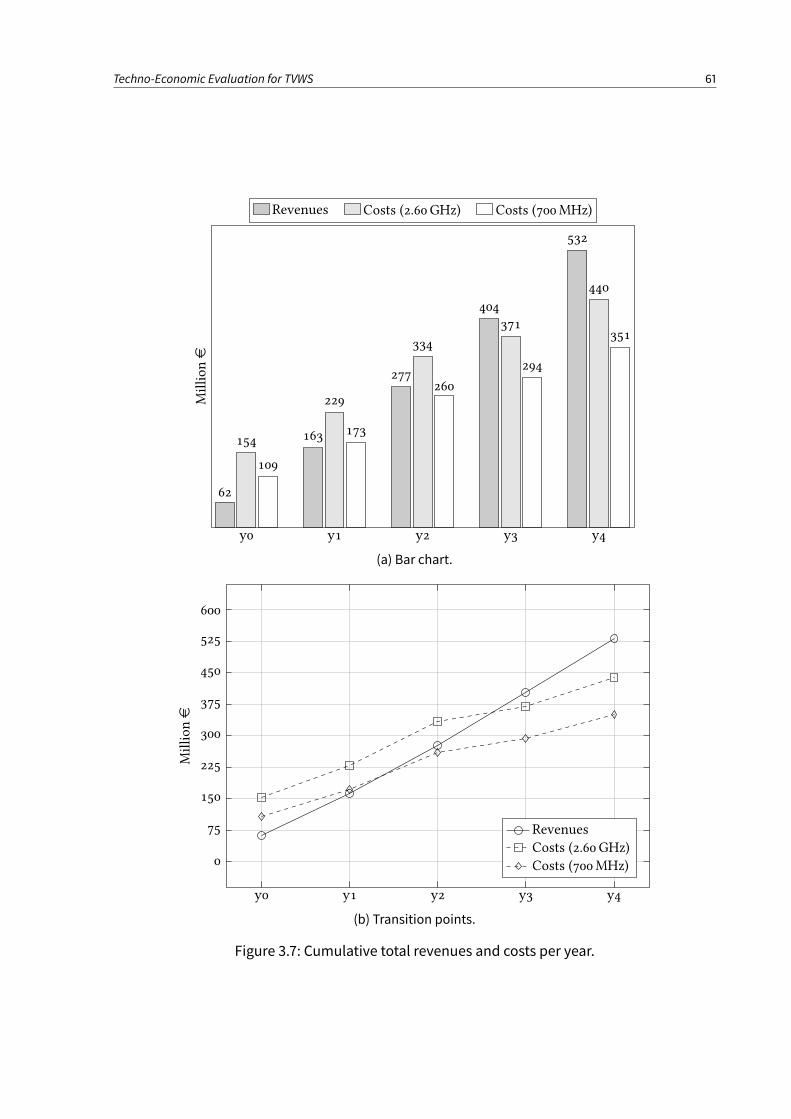
Techno-Economic Evaluation for TVWS 61
y0 y1 y2 y3 y4
62
163
277
404
532
154
229
334
371
440
109
173
260
294
351
Millione
Revenues Costs (2.60 GHz) Costs (700MHz)
(a) Bar chart.
y0 y1 y2 y3 y4
0
75
150
225
300
375
450
525
600
Millione
Revenues
Costs (2.60 GHz)
Costs (700MHz)
(b) Transition points.
Figure 3.7: Cumulative total revenues and costs per year.
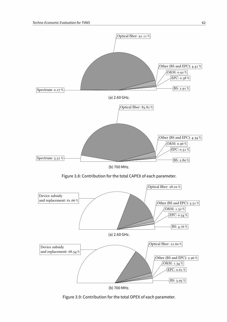
Techno-Economic Evaluation for TVWS 62
BS: 2.91 %
EPC: 0.38 %
O&M: 0.92 %
Other (BS and EPC): 4.41 %
Optical ber: 91.11 %
Spectrum: 0.27 %
(a) 2.60 GHz.
BS: 2.80 %
EPC: 0.51 %
O&M: 0.96 %
Other (BS and EPC): 4.34 %
Optical ber: 85.82 %
Spectrum: 5.51 %
(b) 700MHz.
Figure 3.8: Contribution for the total CAPEX of each parameter.
BS: 4.76 %
EPC: 0.54 %
O&M: 1.52 %
Other (BS and EPC): 3.51 %
Optical ber: 28.02 %
Device subsidy
and replacement: 61.66 %
(a) 2.60 GHz.
BS: 3.95 %
EPC: 0.61 %
O&M: 1.34 %
Other (BS and EPC): 2.96 %
Optical ber: 22.60 %Device subsidy
and replacement: 68.54 %
(b) 700MHz.
Figure 3.9: Contribution for the total OPEX of each parameter.

Techno-Economic Evaluation for TVWS 63
1 253 480 people in y4. The slope in both lines is high, which means that NPV is very sensitiveto the reduction in clients base.
The higher slope presented in the reduction from 30 to 40 % in clients base is derivedfrom the fact that with less clients the operator receives less revenues but, as explained insection 3.2.2, if there is at least one client per borough, one BS (and EPC) needs to be deployedto attend that client; and for a reduction of 40 % in the clients base, the NPV in 2.60GHz isnegative, i.e., the network becomes non-protable.
REF −10% −20% −30% −40%
−40
−15
10
35
60
85
110
135
160
Number of clients
NPV[m
illione]
2.60 GHz
700MHz
Figure 3.10: Total NPV variation by reducing the number of clients.
Figure 3.11 presents the NPV variation while increasing the price of devices. The REF valuesare e80 in y0, e60 in y1, e40 in y2, e30 in y3, and e20 in y4. Since the slope of the lines isnot very high, the NPV is not very sensitive to the increase in the price of devices.
In gure 3.12 it is shown the variation of the total NPV to the increase in device subsidiesthat an operator gives to its clients. The REF value is 50 %. As can be seen, the slope of bothlines is not very high, thus, the NPV is not very sensitive to the increase in the device subsides.Nevertheless, it reveals to be more sensitive than to the increase in price of devices.
In gure 3.13 the variation of NPV to the reduction in ARPU is shown. The REF value ise13. For this case, the slope of the lines is very high, which means that NPV is highly sensitiveto the reduction in the ARPU. As such, the NPV becomes negative if ARPU reduces around13% in the deployment scenario of 2.60GHz, while for 700MHz the reduction must be around32 %. Nevertheless, in both cases the network becomes non-protable. On the other hand, it isclear that NPV is more sensitive to the reduction in ARPU than to the reduction in clients base.
Figure 3.14 shows the NPV variation considering the increase in the price of spectrum. TheREF is e3million for 2.60GHz and e45million for 700MHz. In this result, both lines appearto be nearly horizontal. This means that NPV is not sensitive to the increase in the price ofspectrum. It may seem surprising for 700MHz because, as shown in gure 3.8(b), the priceof spectrum represents 5.51 % of the CAPEX for the reference values. However, if we analyzethe impact of increasing the price of spectrum in CAPEX, we see that its impact in the worst
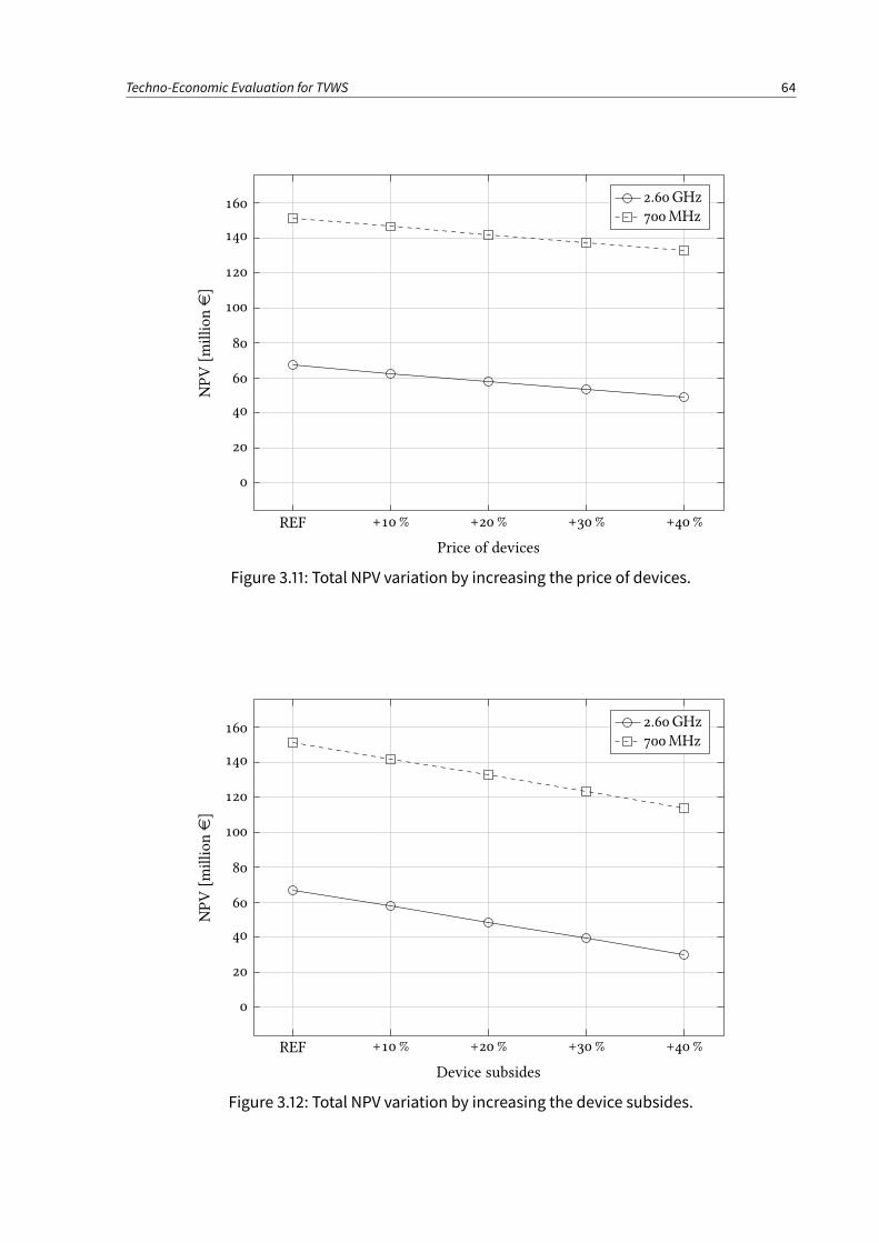
Techno-Economic Evaluation for TVWS 64
REF +10% +20% +30% +40%
0
20
40
60
80
100
120
140
160
Price of devices
NPV[m
illione]
2.60 GHz
700MHz
Figure 3.11: Total NPV variation by increasing the price of devices.
REF +10% +20% +30% +40%
0
20
40
60
80
100
120
140
160
Device subsides
NPV[m
illione]
2.60 GHz
700MHz
Figure 3.12: Total NPV variation by increasing the device subsides.
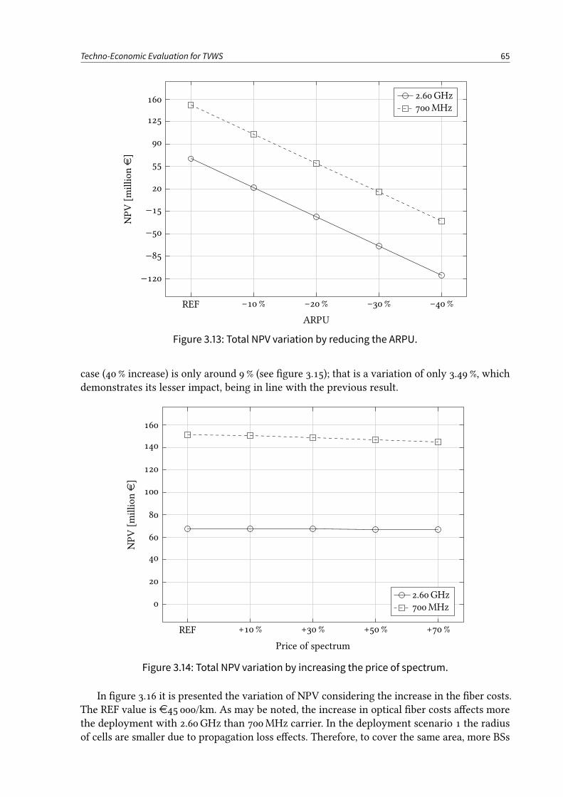
Techno-Economic Evaluation for TVWS 65
REF −10% −20% −30% −40%
−120
−85
−50
−15
20
55
90
125
160
ARPU
NPV[m
illione]
2.60 GHz
700MHz
Figure 3.13: Total NPV variation by reducing the ARPU.
case (40 % increase) is only around 9% (see gure 3.15); that is a variation of only 3.49 %, whichdemonstrates its lesser impact, being in line with the previous result.
REF +10% +30% +50% +70%
0
20
40
60
80
100
120
140
160
Price of spectrum
NPV[m
illione]
2.60 GHz
700MHz
Figure 3.14: Total NPV variation by increasing the price of spectrum.
In gure 3.16 it is presented the variation of NPV considering the increase in the ber costs.The REF value is e45 000/km. As may be noted, the increase in optical ber costs aects morethe deployment with 2.60GHz than 700MHz carrier. In the deployment scenario 1 the radiusof cells are smaller due to propagation loss eects. Therefore, to cover the same area, more BSs
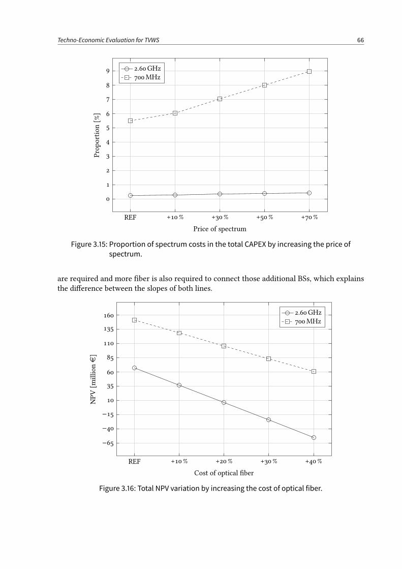
Techno-Economic Evaluation for TVWS 66
REF +10% +30% +50% +70%
0
1
2
3
4
5
6
7
8
9
Price of spectrum
Proportion[%]
2.60 GHz
700MHz
Figure 3.15: Proportion of spectrum costs in the total CAPEX by increasing the price of
spectrum.
are required and more ber is also required to connect those additional BSs, which explainsthe dierence between the slopes of both lines.
REF +10% +20% +30% +40%
−65
−40
−15
10
35
60
85
110
135
160
Cost of optical ber
NPV[m
illione]
2.60 GHz
700MHz
Figure 3.16: Total NPV variation by increasing the cost of optical fiber.
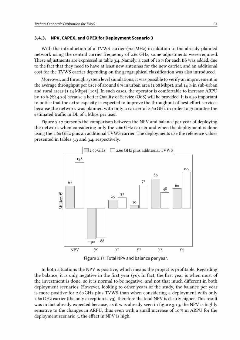
Techno-Economic Evaluation for TVWS 67
3.4.3. NPV, CAPEX, and OPEX for Deployment Scenario 3
With the introduction of a TVWS carrier (700MHz) in addition to the already plannednetwork using the central carrier frequency of 2.60GHz, some adjustments were required.These adjustments are expressed in table 3.4. Namely, a cost of 10 % for each BS was added, dueto the fact that they need to have at least new antennas for the new carrier, and an additionalcost for the TVWS carrier depending on the geographical classication was also introduced.
Moreover, and through system level simulations, it was possible to verify an improvement inthe average throughput per user of around 8% in urban area (1.08Mbps), and 14 % in sub-urbanand rural areas (1.14Mbps) [105]. In such cases, the operator is comfortable to increase ARPUby 10% (e14.30) because a better Quality of Service (QoS) will be provided. It is also importantto notice that the extra capacity is expected to improve the throughput of best eort servicesbecause the network was planned with only a carrier of 2.60GHz in order to guarantee theestimated trac in DL of 1Mbps per user.
Figure 3.17 presents the comparison between the NPV and balance per year of deployingthe network when considering only the 2.60GHz carrier and when the deployment is doneusing the 2.60GHz plus an additional TVWS carrier. The deployments use the reference valuespresented in tables 3.3 and 3.4, respectively.
NPV y0 y1 y2 y3 y4
67
−92
25
10
89
60
138
−88
32
71
48
109
Millione
2.60GHz 2.60GHz plus additional TVWS
Figure 3.17: Total NPV and balance per year.
In both situations the NPV is positive, which means the project is protable. Regardingthe balance, it is only negative in the rst year (y0). In fact, the rst year is when most ofthe investment is done, so it is normal to be negative, and not that much dierent in bothdeployment scenarios. However, looking to other years of the study, the balance per yearis more positive for 2.60GHz plus TVWS than when considering a deployment with only2.60GHz carrier (the only exception is y3), therefore the total NPV is clearly higher. This resultwas in fact already expected because, as it was already seen in gure 3.13, the NPV is highlysensitive to the changes in ARPU, thus even with a small increase of 10 % in ARPU for thedeployment scenario 3, the eect in NPV is high.
Techno-Economic Evaluation for TVWS 68
In gure 3.18 the cumulative revenues and costs per year for the deployment scenario 1 areshown; the same result is expressed in gure 3.19 for the deployment scenario 3. If we look onlyat gure 3.18(a) and gure 3.19(a) we can be tempted to say that the dierence between the twodeployments considering both the revenues and costs is not signicant. However, let us look tothe third year (y2). Only in the case of a deployment for 2.60GHz plus an additional TVWS therevenues bar is slightly above the costs bar for that year; while in the case of a deploymentwith 2.60GHz only, the revenues bar is only clearly above costs bar in the fourth year (y3).
A better visual illustration of the same result is depicted in gure 3.19(b), where the line ofrevenues crosses the line of costs before the third year of deployment, while in gure 3.18(b) itonly happens almost at the end of the third year. In other words, it is clear that an operatorwould recover its investment around one year earlier if it chooses to deploy the networkfollowing a exible spectrum market approach.
Despite the previous results, it is a good idea to determine the main sources of costs in thenetwork. In gure 3.20 the principal contributors to CAPEX and OPEX for the deploymentscenario 3 can be seen. Regarding the CAPEX, it is very similar to gure 3.8(a) that was done fora network with only the 2.60GHz carrier. Actually, this result was expected, because the onlyadded cost to CAPEX is the increase of 10 % in the cost of each BS due to the required additionalantenna to support TVWS. The main dierence may be seen in OPEX where the annual priceof spectrum for TVWS now represents around 12% of the total OPEX. Nevertheless, devicesubsidies and replacement costs still remain as the most important contributor to OPEX.
Although, despite the big impact in OPEX, the price of TVWS does not have a visibleimpact in the total NPV (which remains very positive). This may be explained because withthe reference values, 81 % of the costs are CAPEX while only 19 % are OPEX.
3.4.4. Sensitivity Analysis for Deployment Scenario 3
In addition to the sensitivity analysis already done in section 3.4.2, within this sectionwe provide two more sensitivity analysis, namely to assess the inuence in the total NPV ofincreasing the price of a TVWS carrier and the number of hours/day (in average) that theoperator must pay to use such carrier (or TVWS channel).
In gure 3.21 it is presented the variation of NPV while the price of TVWS increases. TheREF values are: e411/day for urban, e247/day for sub-urban, and e164/day for rural areas. Inboth cases, for the average use of four hours/day or eight hours/day, the slope of the lines isnot very steep; that is the NPV is not very sensitive to the increase in the price of TVWS.
Figure 3.22 shows the variation in NPV while increasing the number of hours/day thatan operator must pay for the use of a TVWS carrier. The REF value is four hours/day, whichrepresents in average the typical use time per day of the year.
As it can be seen, once again, the variation of NPV is not very high (arounde132million forREF to around e113million for 12 hours/day). Since the use of TVWS is to overcome situationsof lack in capacity during busy hours, it does not make sense to use the TVWS during thewhole day. However, even for the worst case, that is when the operator must pay 24 hours/dayfor the use of a TVWS carrier, the value of NPV is e84million, which is clearly above thee64million obtained when considering only a carrier of 2.60GHz.
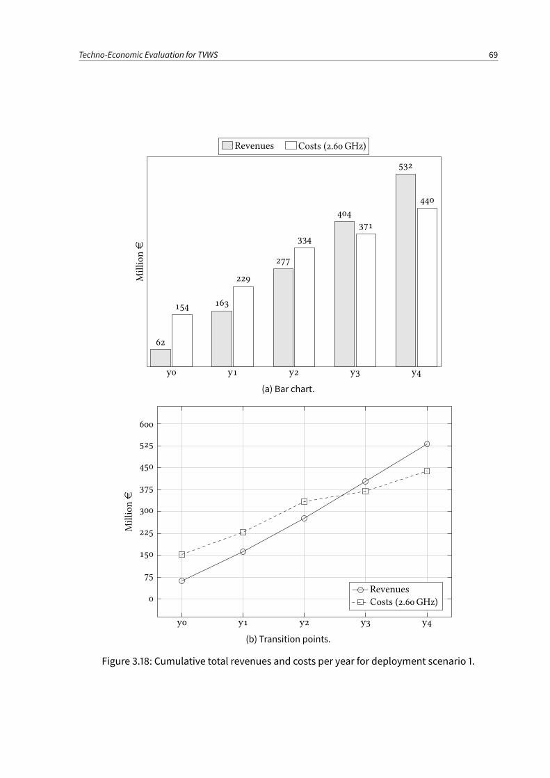
Techno-Economic Evaluation for TVWS 69
y0 y1 y2 y3 y4
62
163
277
404
532
154
229
334
371
440
Millione
Revenues Costs (2.60 GHz)
(a) Bar chart.
y0 y1 y2 y3 y4
0
75
150
225
300
375
450
525
600
Millione
Revenues
Costs (2.60 GHz)
(b) Transition points.
Figure 3.18: Cumulative total revenues and costs per year for deployment scenario 1.
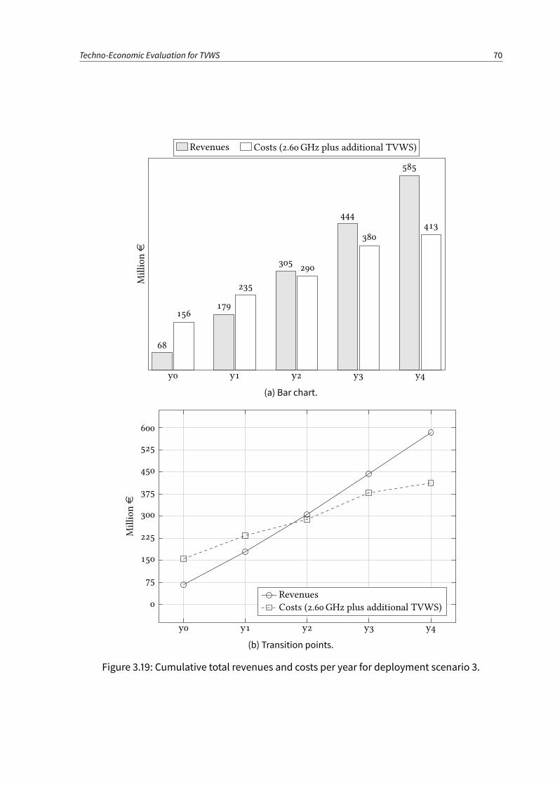
Techno-Economic Evaluation for TVWS 70
y0 y1 y2 y3 y4
68
179
305
444
585
156
235
290
380413
Millione
Revenues Costs (2.60 GHz plus additional TVWS)
(a) Bar chart.
y0 y1 y2 y3 y4
0
75
150
225
300
375
450
525
600
Millione
Revenues
Costs (2.60 GHz plus additional TVWS)
(b) Transition points.
Figure 3.19: Cumulative total revenues and costs per year for deployment scenario 3.
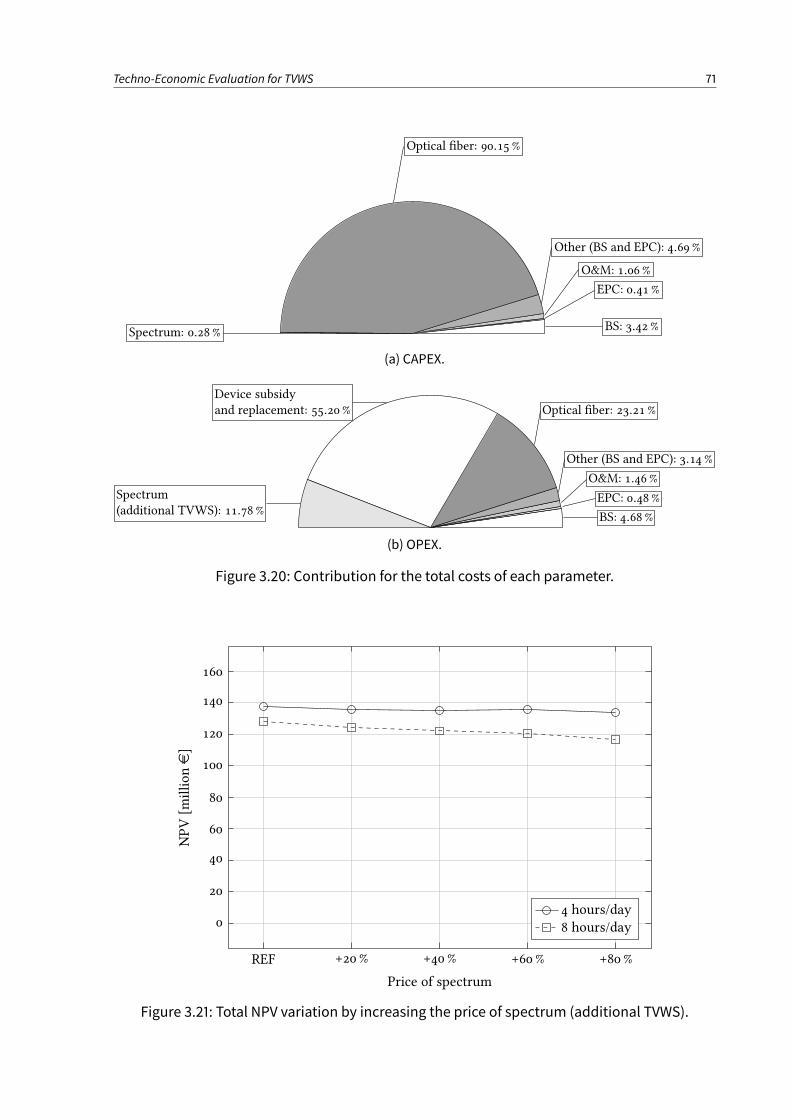
Techno-Economic Evaluation for TVWS 71
BS: 3.42 %
EPC: 0.41 %
O&M: 1.06 %
Other (BS and EPC): 4.69 %
Optical ber: 90.15 %
Spectrum: 0.28 %
(a) CAPEX.
BS: 4.68 %
EPC: 0.48 %
O&M: 1.46 %
Other (BS and EPC): 3.14 %
Optical ber: 23.21 %
Device subsidy
and replacement: 55.20 %
Spectrum
(additional TVWS): 11.78 %
(b) OPEX.
Figure 3.20: Contribution for the total costs of each parameter.
REF +20% +40% +60% +80%
0
20
40
60
80
100
120
140
160
Price of spectrum
NPV[m
illione]
4 hours/day
8 hours/day
Figure 3.21: Total NPV variation by increasing the price of spectrum (additional TVWS).
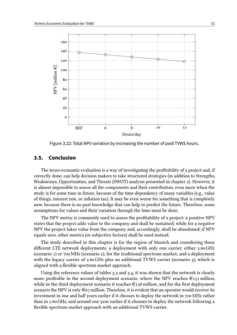
Techno-Economic Evaluation for TVWS 72
REF 6 8 10 12
0
20
40
60
80
100
120
140
160
Hours/day
NPV[m
illione]
Figure 3.22: Total NPV variation by increasing the number of paid TVWS hours.
3.5. Conclusion
The tecno-economic evaluation is a way of investigating the protability of a project and, ifcorrectly done, can help decision makers to take structured strategies (in addition to Strengths,Weaknesses, Opportunities, and Threats (SWOT) analysis presented in chapter 2). However, itis almost impossible to assess all the components and their contribution, even more when thestudy is for some time in future, because of the time-dependency of many variables (e.g., valueof things, interest rate, or ination tax). It may be even worse for something that is completelynew, because there is no past knowledge that can help to predict the future. Therefore, someassumptions for values and their variation through the time must be done.
The NPV metric is commonly used to assess the protability of a project: a positive NPVstates that the project adds value to the company and shall be sustained; while for a negativeNPV the project takes value from the company and, accordingly, shall be abandoned; if NPVequals zero, other metrics (or subjective factors) shall be used instead.
The study described in this chapter is for the region of Munich and considering threedierent LTE network deployments: a deployment with only one carrier, either 2.60GHz(scenario 1) or 700MHz (scenario 2), for the traditional spectrum market; and a deploymentwith the legacy carrier of 2.60GHz plus an additional TVWS carrier (scenario 3), which isaligned with a exible spectrum market approach.
Using the reference values of tables 3.3 and 3.4, it was shown that the network is clearlymore protable in the second deployment scenario, where the NPV reaches e151million,while in the third deployment scenario it reaches e138million, and for the rst deploymentscenario the NPV is only e67million. Therefore, it is evident that an operator would recover itsinvestment in one and half years earlier if it chooses to deploy the network in 700MHz ratherthan in 2.60GHz, and around one year earlier if it chooses to deploy the network following aexible spectrum market approach with an additional TVWS carrier.
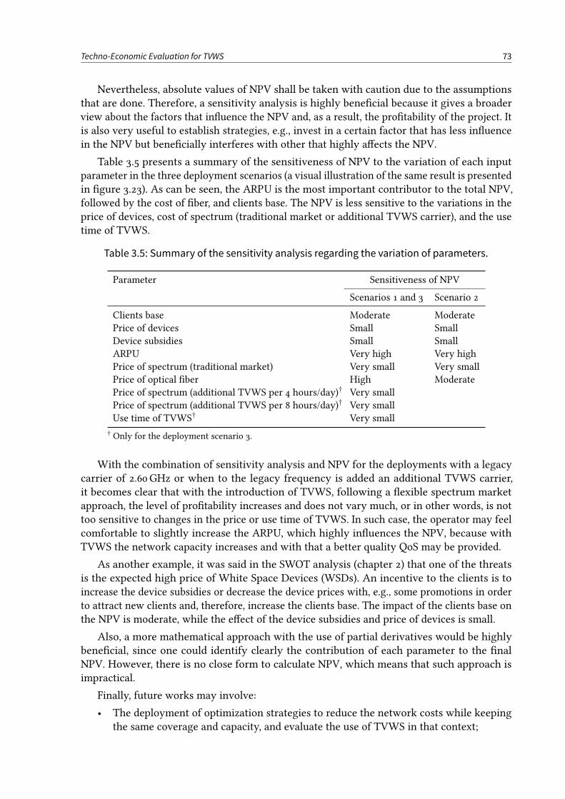
Techno-Economic Evaluation for TVWS 73
Nevertheless, absolute values of NPV shall be taken with caution due to the assumptionsthat are done. Therefore, a sensitivity analysis is highly benecial because it gives a broaderview about the factors that inuence the NPV and, as a result, the protability of the project. Itis also very useful to establish strategies, e.g., invest in a certain factor that has less inuencein the NPV but benecially interferes with other that highly aects the NPV.
Table 3.5 presents a summary of the sensitiveness of NPV to the variation of each inputparameter in the three deployment scenarios (a visual illustration of the same result is presentedin gure 3.23). As can be seen, the ARPU is the most important contributor to the total NPV,followed by the cost of ber, and clients base. The NPV is less sensitive to the variations in theprice of devices, cost of spectrum (traditional market or additional TVWS carrier), and the usetime of TVWS.
Table 3.5: Summary of the sensitivity analysis regarding the variation of parameters.
Parameter Sensitiveness of NPV
Scenarios 1 and 3 Scenario 2
Clients base Moderate ModeratePrice of devices Small SmallDevice subsidies Small SmallARPU Very high Very highPrice of spectrum (traditional market) Very small Very smallPrice of optical ber High ModeratePrice of spectrum (additional TVWS per 4 hours/day)† Very smallPrice of spectrum (additional TVWS per 8 hours/day)† Very smallUse time of TVWS† Very small
† Only for the deployment scenario 3.
With the combination of sensitivity analysis and NPV for the deployments with a legacycarrier of 2.60GHz or when to the legacy frequency is added an additional TVWS carrier,it becomes clear that with the introduction of TVWS, following a exible spectrum marketapproach, the level of protability increases and does not vary much, or in other words, is nottoo sensitive to changes in the price or use time of TVWS. In such case, the operator may feelcomfortable to slightly increase the ARPU, which highly inuences the NPV, because withTVWS the network capacity increases and with that a better quality QoS may be provided.
As another example, it was said in the SWOT analysis (chapter 2) that one of the threatsis the expected high price of White Space Devices (WSDs). An incentive to the clients is toincrease the device subsidies or decrease the device prices with, e.g., some promotions in orderto attract new clients and, therefore, increase the clients base. The impact of the clients base onthe NPV is moderate, while the eect of the device subsidies and price of devices is small.
Also, a more mathematical approach with the use of partial derivatives would be highlybenecial, since one could identify clearly the contribution of each parameter to the nalNPV. However, there is no close form to calculate NPV, which means that such approach isimpractical.
Finally, future works may involve:
• The deployment of optimization strategies to reduce the network costs while keepingthe same coverage and capacity, and evaluate the use of TVWS in that context;
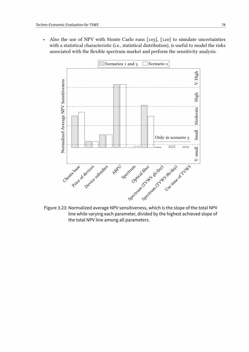
Techno-Economic Evaluation for TVWS 74
• Also the use of NPV with Monte Carlo runs [103], [120] to simulate uncertaintieswith a statistical characteristic (i.e., statistical distribution), is useful to model the risksassociated with the exible spectrum market and perform the sensitivity analysis.
Clients base
Priceofdevices
Devicesubsidies
ARPU
Spectrum
Opticalber
Spectrum
(TVWS4h/day)
Spectrum
(TVWS8h/day)
UsetimeofTVWS
Norm
alized
AverageNPVSensitiveness
Scenarios 1 and 3 Scenario 2
V.small
Small
Moderate
High
V.H
igh
Only in scenario 3
Figure 3.23: Normalized average NPV sensitiveness, which is the slope of the total NPV
line while varying each parameter, divided by the highest achieved slope of
the total NPV line among all parameters.
PART II
D2D Communications
This part is devoted to the research topic of Device-to-Device (D2D). The part comprisesthe following chapters:
• Chapter 4. Neighbor Discovery Using Power Vectors for D2D Communications: in thischapter it is proposed a network-assisted technique to discover D2D-capable neighborsof a rst Mobile Station (MS) based on the power measurements already available in thenetwork. Results show that with the network help, the time to detect all neighbors perMS is signicantly reduced, leaving more time available for data transmission;
• Chapter 5. Band Selection for D2D Communications: in this chapter a novel co-channelinterference mitigation algorithm is investigated. The algorithm selects the Downlink(DL) or Uplink (UL) band to be reused by the D2D communication using a radio distancemetric. Results proved that interference is mitigated in both communication directions,allowing the coexistence of both cellular and D2D modes, which extends the commonrecommendation of just reusing the UL band for the D2D links.
75
CHAPTER 4
Neighbor Discovery Using Power Vectors for D2D
Communications
The new Device-to-Device (D2D) communication is seen as a promising technology toincrease the capacity of current wireless systems without extra electromagnetic spectrum
bands. However, before starting a D2D communication, Mobile Stations (MSs) must be awareof their neighbors, through a discovery process. While operating in cellular networks, suchprocess may benet from the network assistance. In this chapter, we propose a method basedon the available network power measurements to improve the discovery process. Resultsdemonstrate that our proposal is less complex but still outperforms traditional methods whenconsidering the time to detect all neighbors.
4.1. Introduction
The notable popularity of smartphones and tablets alongwith the increasing demand for richmultimedia services and the scarcity of electromagnetic spectrum has motivated the researchof technologies that are able to improve the capacity of wireless systems without requiringextra spectrum bands. In this context, D2D communication represents a promising technologythat has attracted the attention of scientic community in the last couple of years [26].
As discussed in chapter 1, D2D communication is a new type of direct wireless communi-cation between two or more network radio nodes, hereafter generally referred as MSs1, thatexploits the proximity between them to achieve very high data rates and low delays, with areduced power consumption. But, it comes with the cost of introducing additional interference,which is seen as the main drawback. Benets and challenges of D2D communications, especiallyin cellular networks, are discussed in, e.g., [26], [27], [121].
However, before commencing a D2D communication, each D2D-capable MS2 must have theknowledge of its neighbors, i.e., other D2D-capable MSs in the vicinity of the former with whichit may directly communicate with. Ideally, MSs shall discover their neighbors as quickly aspossible, which enables them to save power. Also, a speedy discovery allows routing and otherprotocols to quickly start their execution, without signicantly decrease the MSs’ operationtime [122], [123]. Moreover, the discovery shall be adaptive from sparse environments, withjust a few MSs, to densely populated places, with large number of MSs [124].
1 The method presented in this chapter can be applied to any wireless network and not strictly to Long TermEvolution (LTE) systems, thus we adopted a more general terminology, as Mobile Station (MS) and Base Station(BS). Nevertheless, MS refers to User Equipment (UE) while Base Station (BS) refers to Evolved Node B (eNB) inLTE family standards.
2 A MS that can operate in cellular or D2D mode (one at time), but preferably uses D2D mode.
76
Neighbor Discovery Using Power Vectors for D2D Communications 77
Therefore, the main problem herein is to determine the pool of neighbors for each D2D-capable MS: if the process does not occur or no neighbors are found, the D2D communicationwill not happen; simply because the MS is not aware of other surrounding D2D-capable MSs.
4.1.1. Neighbor Discovery
Neighbor discovery, as described in [123], is the determination of all MS in the networkwith which a given MS may directly communicate with, i.e., establish a D2D communication.
Immediately after the ad hoc network deployment, a MS has no knowledge about the otherMS in its transmission range and needs to discover its neighbors. Therefore, the neighbordiscovery process is one of the rst steps in the conguration of large wireless networks [125].The problem becomes crucial in self-organizing networks without preexisting infrastructure.Nevertheless, the number of neighbors is typically orders of magnitude smaller than the sizeof all network interface addresses, so neighbor discovery is by nature compressed sensing (orsparse discovery) [126]. In addition, neighbor discovery may also be the solution for partnerselection in cooperative wireless networks.
The neighbor discovery shall not signicantly decrease the operation time of MSs and bescalable to very sparse environments, with few nodes, to crowded places. In a crowded place,the discovery process becomes challenging as well as keeping the energy consumption low. Insparse environments it may happen that there are no neighbors and the scanning process mustnot completely drain the MS’s battery [124]. Furthermore, energy eciency in maintaining thenetwork and guaranteeing a low duty cycle [127] are also desirable.
The nal step in the D2D link establishment procedure is to trigger a beacon between theD2D server and client to evaluate the actual quality of the channel and build the requiredrouting tables. In LTE-like networks, the D2D link quality is reported to the eNB and serves asthe basic input to mode selection, i.e., select cellular or D2D communication modes [35].
Disambiguation
One may confuse the neighbor discovery (sometimes also referred in literature as peerdiscovery) in the context of D2D communications with BitTorrent services3 and their peerdiscovery mechanism. First, there is a clear dierence in the concept, studied problems, andproposed solutions; second, the D2D communication focus the physical and link layers, namelyMediumAccess Control (MAC) sublayer; while BitTorrent is a service and, therefore, consideredin upper layers (network, transport, and application).
Moreover, D2D communications are being proposed for ad hoc wireless networks, and alsofor the cellular domain as an underlay (secondary) network of the primary one [27]. Hence, theradio nodes participating in D2D communications form a network that is capable of exchangingdata: transfer les, voice conversation, audio and video streaming, or other kind of services.
The D2D-related mechanisms are somehow similar to the ones that do exist in Bluetoothtechnology4—peer discovery and device pairing—where the so-called inquiry process allowsa potential master MS to identify other MSs in range that wish to participate in a piconet,
3 BitTorrent is a Peer to Peer (P2P) le sharing protocol used for distributing large amounts of data over theInternet [128].
4 See http://bluetooth.org.
Neighbor Discovery Using Power Vectors for D2D Communications 78
whereas the paging process allows the master MS to establish links towards the desired slaveMS [26].
Algorithms Classification
According to [125] the neighbor discovery algorithms can be classied in two maincategories: randomized or deterministic. However, many other divisions may also apply,depending on the type of, e.g., technology, network organization, focused layers, antennas,protocols, or signaling methods. A good discussion on neighbor discovery algorithms (namelyfor ad hoc networks) and their classication can be found in [129], [130].
Considering the type of network and the knowledge of its structure, the neighbor discoveryalgorithms may be used in deterministic or random networks. In a deterministic network, thestructure is mostly static andwell-known, therefore reorganizations are infrequent. On the otherhand, for random networks, the neighbor discovery algorithms must cope with uncertaintyand common reorganizations due to, e.g., entrance/exit of MSs and their movement, and thusparameters may drastically change between sessions [27], [122], [131]. For random networks,the list of neighbors and routing tables shall at least be updated before the establishment ofeach data link, while for deterministic networks, the bootstrap conguration (this is, whenMSs are turned on) may be sucient to keep lists updated.
Neighbor discovery protocols are sometimes generally classied as one-way neighbordiscovery or handshake-based neighbor discovery [132]; they can also be classied as powerdetection or protocol-oriented, respectively. Power detection neighbor discovery requiresthat each MS periodically sends out advertising packets (in random or dened directions) toannounce its presence, and neighbors are discovered by receiving their advertising packets [124].For protocol-oriented neighbor discovery, a MS needs to provide active response to the senderafter receiving an advertising packet from an unknown neighbor. Protocol-oriented neighbordiscovery is usually implemented at MAC sublayer, while power detection neighbor discoveryis in physical layer. Relying only on power detection, i.e., carrier sensing at physical layer, mayled to undetected neighbors and the hidden node problem.
Actually, the hidden node problem is one of the main sources of packet collision in wirelessnetworks: when two or more MSs attempt to transmit a packet across the network at the sametime, a packet collision occurs. Although, if a collision happens and no recover is possible,the detection of neighbors can be compromised. Collisions may be avoided by the use ofwide-spaced channels, carrier sensing mechanism (which are implemented at MAC sublayer),or at modulation level, like using Orthogonal Frequency Division Multiplexing (OFDM)-basedschemes [130], [133]. Moreover, synchronous (or slotted) detection may also be implementedto mitigate collisions and, therefore, all MSs transmit following a common reference frame,which is allowed with the distribution of a local clock [129]. In asynchronous detection, thereis no cooperation between MS. Hence, their transmission slots are misaligned which conductto detections up two times slower than in the synchronous counterpart [125], [134].
Other common division to evaluate the probability and required time to detect all neigh-bors is the distinction between randomized and deterministic neighbor discovery [125]. Inrandomized neighbor discovery, each MS transmits at randomly chosen times and neighborsare detected with high probability within a predened timeout. In a deterministic neighbordiscovery, each MS transmits according to a predetermined schedule which allows the detectionof all neighbors during the timeout. In deterministic neighbor discovery, the transmission mayoccur, e.g., like in the well-known token ring protocol that exists for wired networks; where
Neighbor Discovery Using Power Vectors for D2D Communications 79
token-possession grants the possessor permission to transmit on the medium, i.e., when aMS transmits, the other MSs listen, thus avoiding collision problems. In randomized neighbordiscovery, collisions are likely to occur. In [125], [127] the detection of neighbors is reduced tocoupon collector’s problem, where the time to detect all neighbors is lower and upper boundedwith closed form expressions.
Regarding the type and number of antennas, two division can be considered: the use ofomnidirectional or directional antennas, and Single Input Single Output (SISO) orMultiple Input,Multiple Output (MIMO) schemes. Many neighbor discover protocols have been proposed thatuse directional antennas. Directional antennas concentrate their beams according to specicdirections, which enables selectivity in the reception (along with the increase of Signal toInterference-plus-Noise Ratio (SINR)) and for a given transmission power, the communicationrange is greatly extended [122]. However, the hidden node problem [135] and deafness [136]due to misalignment in transmitter and receiver’s antennas are common problems. As such,protocol design using directional antennas is a challenging problem, while neighbor discoveryis seen as relatively simpler problem when omnidirectional antennas are used because a simplebroadcast can reach all MSs within the transmission range [131].
For the spatial diversity, conventional MIMO schemes require that both the transmitter andreceiver must be equipped with multiple antenna arrays. In practice, however, many MSs maynot be able to support multiple antennas due to size, cost, and/or hardware limitations. For D2Dcommunications an alternative approach is to use cooperative MIMO: that is to group multipleMS into virtual antenna arrays to emulate MIMO communications [137]. For example, whena target MS temporarily suers from bad channel conditions or requires relatively high rateservice, its neighboring MSs can help to provide multi-hop coverage or increase the data rateby relaying information to the target MS, or even detect MSs that were inaccessible in otherway. Typical neighbor discovery algorithms use SISO, thus they can only provide one-hopinformation.
Finally, neighbor discovery algorithms can also be divided according to the type of networkfor which they were projected. In the self-sucient (or unsupervised) neighbor discoveryalgorithms, the MSs rely only on themselves to detect neighbors. There is no central coordinatorMS neither a central database of yet discovered MSs. Typically, self-sucient algorithmsare implemented in wireless ad hoc networks. On the other hand, the network-assisted (orsupervised) neighbor discovery is likely to be implemented in typical cellular networks, wherethe access network (and core network) cooperates with MSs to detect D2D candidates [27]. Innetwork-assisted neighbor discovery, the identication of D2D candidates can be done usinga-priori or a-posteriori schemes [26]. The a-priori scheme is used if MS or network detects D2Dcandidates just before commencing the communication data session between MSs in cellularmode; while a-posteriori scheme is employed if D2D candidates are only detected during theongoing cellular communication sessions.
4.1.2. Decentralized vs. Network-Assisted Discovery
As such, each MS may employ a neighbor discovery mechanism without being network-assisted. This is a decentralized beaconing mechanism [138], [139], where each MS acts only onits own. The natural improvement is to combine the beaconing mechanism with an exchangingprotocol, where the Identitys (IDs) of already detected neighbors are shared between all MSsin the neighborhood [131]. However, both approaches have the following problems:
Neighbor Discovery Using Power Vectors for D2D Communications 80
• Time to discover and stopping criteria: if the discovery process takes too long, it may beuseless, since no time is left for data transmission, and good stopping criteria are dicultto be eectively dened [125]. This is especially relevant because the surroundingenvironment is unknown and the discovery may happen from sparse to crowdedenvironments [124], [126];
• Power consumption: the discovery process may completely discharge the MS’s battery,namely if the number of possible neighbors is not prior-known and stopping criteriaare not correctly implemented [124], [140];
• New protocol: for the beaconing sequence, and particularly in the case of exchanginginformation about the already known (discovered) neighbors, a new protocol needs tobe dened and implemented [141], implying more network load on signaling;
• HiddenMS problem: relying only on power detection at physical layer, and, for directionalantennas, the misalignment between transmitter and receiver’s antennas, may lead toundetected neighbors [135];
• Fake MS attack: security attacks may happen from a MS which fakes its ID and pretendsto be another.
In order to overcome the problems mentioned above, MSs may be network-assisted [26],[124], [140], [142] to determine the pool of their neighbors, speeding up the discovery processalong with its accuracy. Therefore the proposed neighbor discovery method of this thesis, whichis described in section 4.2, is an a-priori network-assisted method based on power detection.
The rest of the chapter is organized as follows: in section 4.2 a detailed explanation aboutpower vectors and the neighborhood matrix is given, in section 4.3 the system model used insimulations is presented, in section 4.4 the main results are shown and discussed, in section 4.5the single-cell scenario described in section 4.2 is generalized for the multi-cell case, and insection 4.6 the chapter conclusions are drawn.
4.2. Power Vectors and Neighborhood Matrix
In this section we focus on the detailed explanation about power vectors and how toconstruct the neighborhood matrix. For this, the explanation below is based on gure 4.1 thatpresents a set of messages exchanged between the serving BS and D2D-capable MSs.
4.2.1. Collecting Power Measurements from Neighbor Cell List
All MSs while operating in structured networks, as the case of cellular systems, need toperform a set of measurements. One of the very basic of those measurements is the receivedpower from their serving BS. Furthermore, MSs must also perform power measurements onthe pilots of vicinity cells (phase 1 of gure 4.1) and report back those values to the serving BS(phase 2 of gure 4.1). This procedure is mandatory in any cellular system because of mobilityand cell-reselection, due to, e.g., handover and resource allocation reasons. Additionally, atimestamp can be associated to each set of power measurements and if a power measure isdetected to be too old (outside a given useful lifetime period), it can be discarded and a newmeasurement requested.
Moreover, each BS knows its neighbor cells which are stored in a list, commonly describedas Neighbor Cell List (NCL) or monitored set. Note that the model is easily extensible to other
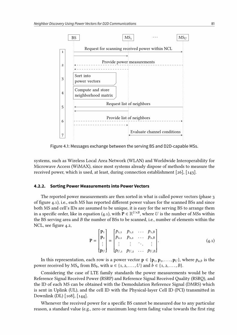
Neighbor Discovery Using Power Vectors for D2D Communications 81
BS MS1 MSU
1
2
3
4
5
6
7
· · ·
Request for scanning received power within NCL
Provide power measurements
Sort into
power vectors
Compute and store
neighborhood matrix
Request list of neighbors
Provide list of neighbors
Evaluate channel conditions
Figure 4.1: Messages exchange between the serving BS and D2D-capable MSs.
systems, such as Wireless Local Area Network (WLAN) and Worldwide Interoperability forMicrowave Access (WiMAX), since most systems already dispose of methods to measure thereceived power, which is used, at least, during connection establishment [26], [143].
4.2.2. Sorting Power Measurements into Power Vectors
The reported power measurements are then sorted in what is called power vectors (phase 3of gure 4.1), i.e., each MS has reported dierent power values for the scanned BSs and sinceboth MS and cell’s IDs are assumed to be unique, it is easy for the serving BS to arrange themin a specic order, like in equation (4.1), with P ∈ RU×B , whereU is the number of MSs withinthe BS serving area and B the number of BSs to be scanned, i.e., number of elements within theNCL, see gure 4.2,
P =
p1p2...
pU
=
p1,1 p1,2 . . . p1,Bp2,1 p2,2 . . . p2,B...
.... . .
...
pU ,1 pU ,2 . . . pU ,B
. (4.1)
In this representation, each row is a power vector p ∈ p1, p2, . . . , pU , where pu,b is thepower received by MSu from BSb , with u ∈ 1, 2, . . . ,U and b ∈ 1, 2, . . . ,B.
Considering the case of LTE family standards the power measurements would be theReference Signal Received Power (RSRP) and Reference Signal Received Quality (RSRQ), andthe ID of each MS can be obtained with the Demodulation Reference Signal (DMRS) whichis sent in Uplink (UL), and the cell ID with the Physical-layer Cell ID (PCI) transmitted inDownlink (DL) [108], [144].
Whenever the received power for a specic BS cannot be measured due to any particularreason, a standard value (e.g., zero or maximum long-term fading value towards the rst ring
Neighbor Discovery Using Power Vectors for D2D Communications 82
of interfering cells) may be used to ll the corresponding gap in the power vector so that themethod is still applicable. Additionally, this value can be controlled, limiting the number offalse neighbors and maximizing the number of real neighbors.
Also, the received power from the serving BS is orders of magnitude greater than thereceived power from other BSs. Thus, to not bias/polarize the results, the received power fromthe serving BS shall be removed from the power vector of each MS (i.e., set to zero).
4.2.3. Building the Neighborhood Matrix
When values are organized in the form of power vectors (phase 3 of gure 4.1), a crosscorrelation metric, ρ, is used to determine the correlation between them. Therefore, taking twodierent power vectors and dening a correlation threshold, PTH, two cases may happen:
• The correlation is high, i.e., ρ > PTH. In this case, MSs are considered neighbors becausetheir set of measurements is very similar, so it is likely to happen that they are in physicalproximity5;
• The correlation is low, i.e., ρ ≤ PTH. In this case, MSs are not considered as neighborsbecause their set of measurements is not similar, hence it is likely to happen that theyare far away from each other.
Clearly, PTH may assume values in the range of zero to one. In one hand, and since weseek to nd high correlated vectors, correlation values below 0.5 are not relevant, while above0.5 may indicate that two MSs are potential neighbors. On the other hand, if the correlationthreshold is set too close to one, eventually many neighbors will be discarded just because theirset of measurements dier in very few elements, while a PTH too close to 0.5 may translate inmore false neighbors (and wasted neighbor detection time). Thus, a reasonable value for thecorrelation threshold shall be around 0.75.
The next step is to calculate the cross correlation metric among all power vectors. A possiblemetric is dened in equation (4.2).
ρx ,y =
⟨
x
‖x‖,y
y
⟩
, and x , y ∈ 1, 2, . . . ,U , (4.2)
where ρx ,y is the normalized cross correlation for power vectors x , y ∈ p1, p2, . . . , pU ;or in other words, x and y are the contents of two dierent rows of matrix P. 〈·, ·〉 is theinner product dened as
⟨
i, j⟩
=
∑Kk=1 ik jk and ‖·‖ is the l2 norm as ‖i‖ =
√∑K
k=1 |ik |2, with
i =[i1 i2 · · · iK
]and j =
[j1 j2 · · · jK
].
Moreover, since x and y are composed by non-negative quantities, ρx ,y will range betweenzero (non-correlated) and one (very high correlated). Finally, the neighborhood matrix, shownin equation (4.3), is constructed and stored in the BS (phase 4 of gure 4.1) as follows:
• If the correlation between MSx and MSy is high, they are tagged as neighbors, and ρx ,ylls the corresponding (x ,y) and (y,x ) indexes (note that ρx ,y = ρy,x );
• Otherwise, MSx and MSy are tagged as non-neighbors, and a zero lls the corresponding(x ,y) and (y,x ) indexes.
5 The real position within the cell is most of the times unavailable. However, cellular links with similar channelsdo have similar propagation eects related with distance, path blockage, and motion.
Neighbor Discovery Using Power Vectors for D2D Communications 83
Ω =
0 w1,2 . . . w1,U
w2,1 0 . . . w2,U...
.... . .
...
wU ,1 wU ,2 . . . 0
, (4.3)
with
wx ,y =
ρx ,y, if x , y and ρx ,y > PTH,
0, otherwise.
Note that matrix Ω ∈ [0, 1]U×U is symmetric, thus only its lower or upper trianglesmay be used, e.g., for saving storage space. Also, the proposed normalized cross correlationmetric expressed as the normalized inner product between two power vectors is one possiblecorrelation metric, but other metrics can be used instead, that are easily found in literature(e.g., see [145, section 9.6] or the Pearson product-moment correlation coecient). Similarly,instead of using the real correlation value in matrix Ω, ones can be stored whenever x , y andρx ,y > PTH, obtaining a binary matrix. Withal, by storing real values, they may be used to sortthe list of neighbors of a MS, improving routing protocols in multicast or broadcast scenarios.
4.2.4. Storage and Exchange of Neighborhood Matrix
Next, the corresponding row or the full neighborhood matrix is delivered to MSs uponrequest (phases 5 and 6 of gure 4.1). Moreover, the D2D link must be evaluated beforecommencing a D2D communication (phase 7 of gure 4.1) by any means. For example, theD2D link may be evaluated using the beaconing approach with a specic training sequence. Inthe results, section 4.4, it is done using a Markov chain.
Additionally, regarding the running time for the message owchart in gure 4.1 it can besettled in the following basis:
• Phases 1 to 4: may be done at every 200ms to 1 s, or 200 to 1000 Transmission TimeIntervals (TTIs) [143];
• Phases 5 to 7: may be done at each new service request or whenever the MS is scheduled.
4.3. SystemModel and Simulation Framework
In this section we describe the models and simulation framework that were adopted toevaluate the system performance. Simulations are divided in two main parts: in the rst part,the simulation scenario is built and the neighborhood matrix is computed as described insection 4.2; and in the second part, each D2D-capable MS uses the direct link to perform thedetection of its neighbors being network-assisted or not.
4.3.1. Cellular Scenario
Consider a network where each BS is placed at the center of a site, which is representedby a regular hexagon. This scenario corresponds to a regular multi-cell network as presentedin gure 4.2. The urban-microcell propagation environment is used, where each site is asingle-cell [146]. Therefore, the multi-cell scenario has B cells and each one serves U MSsuniformly dropped over its coverage area. Moreover, all MSs and BSs are equipped with a singleomnidirectional antenna [147].
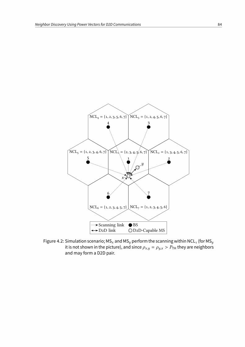
Neighbor Discovery Using Power Vectors for D2D Communications 84
x
y
2
34
5
6 7
1
NCL1 = 2, 3, 4, 5, 6, 7 NCL2 = 1, 3, 4, 5, 6, 7
NCL3 = 1, 2, 4, 5, 6, 7NCL4 = 1, 2, 3, 5, 6, 7
NCL5 = 1, 2, 3, 4, 6, 7
NCL6 = 1, 2, 3, 4, 5, 7 NCL7 = 1, 2, 3, 4, 5, 6
Scanning link BS
D2D link D2D-Capable MS
Figure 4.2: Simulation scenario;MSx andMSy perform the scanningwithinNCL1 (forMSyit is not shown in the picture), and since ρx ,y = ρy,x > PTH they are neighbors
andmay form a D2D pair.
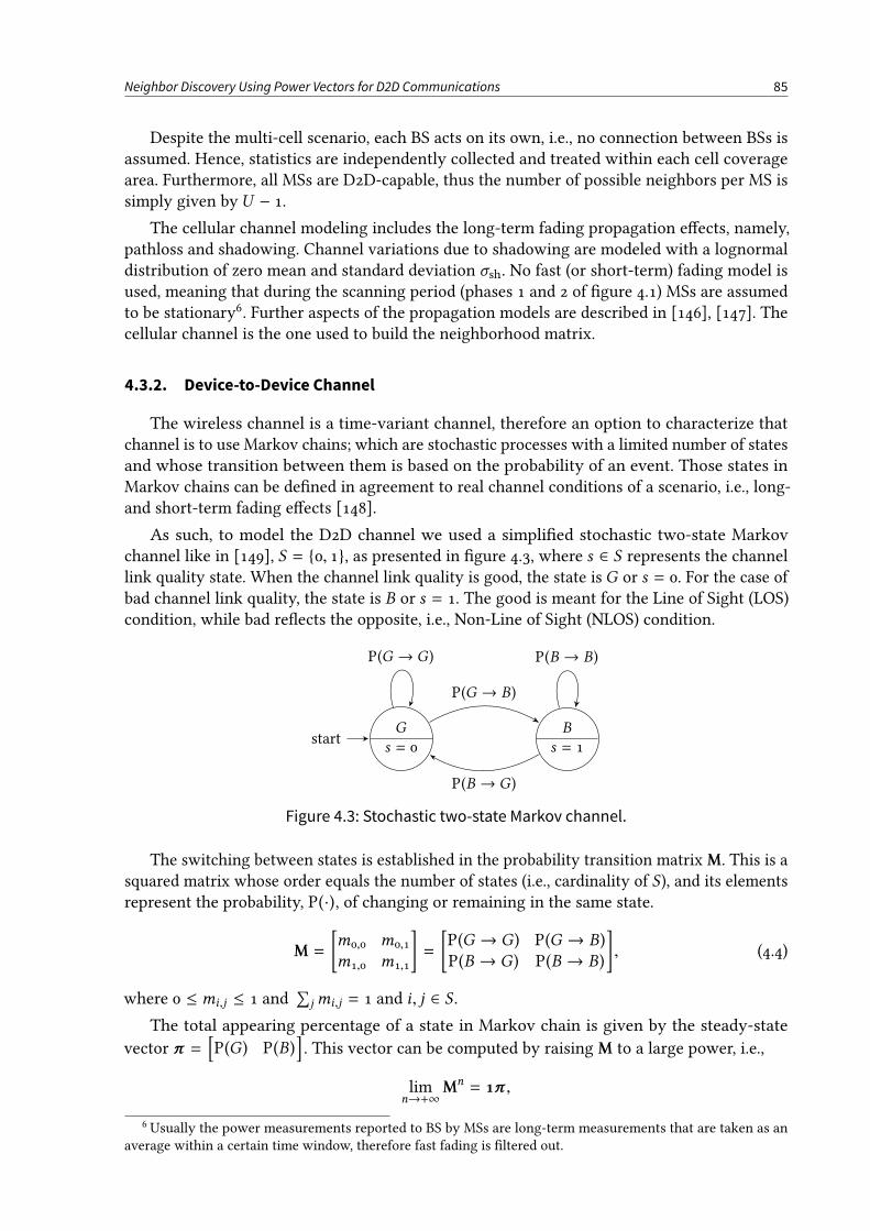
Neighbor Discovery Using Power Vectors for D2D Communications 85
Despite the multi-cell scenario, each BS acts on its own, i.e., no connection between BSs isassumed. Hence, statistics are independently collected and treated within each cell coveragearea. Furthermore, all MSs are D2D-capable, thus the number of possible neighbors per MS issimply given byU − 1.
The cellular channel modeling includes the long-term fading propagation eects, namely,pathloss and shadowing. Channel variations due to shadowing are modeled with a lognormaldistribution of zero mean and standard deviation σsh. No fast (or short-term) fading model isused, meaning that during the scanning period (phases 1 and 2 of gure 4.1) MSs are assumedto be stationary6. Further aspects of the propagation models are described in [146], [147]. Thecellular channel is the one used to build the neighborhood matrix.
4.3.2. Device-to-Device Channel
The wireless channel is a time-variant channel, therefore an option to characterize thatchannel is to use Markov chains; which are stochastic processes with a limited number of statesand whose transition between them is based on the probability of an event. Those states inMarkov chains can be dened in agreement to real channel conditions of a scenario, i.e., long-and short-term fading eects [148].
As such, to model the D2D channel we used a simplied stochastic two-state Markovchannel like in [149], S = 0, 1, as presented in gure 4.3, where s ∈ S represents the channellink quality state. When the channel link quality is good, the state isG or s = 0. For the case ofbad channel link quality, the state is B or s = 1. The good is meant for the Line of Sight (LOS)condition, while bad reects the opposite, i.e., Non-Line of Sight (NLOS) condition.
G
s = 0start
B
s = 1
P(G → G ) P(B → B)
P(G → B)
P(B → G )
Figure 4.3: Stochastic two-state Markov channel.
The switching between states is established in the probability transition matrixM. This is asquared matrix whose order equals the number of states (i.e., cardinality of S), and its elementsrepresent the probability, P(·), of changing or remaining in the same state.
M =
[m0,0 m0,1
m1,0 m1,1
]=
[P(G → G ) P(G → B)
P(B → G ) P(B → B)
], (4.4)
where 0 ≤ mi,j ≤ 1 and∑
jmi,j = 1 and i, j ∈ S .The total appearing percentage of a state in Markov chain is given by the steady-state
vector π =[P(G ) P(B)
]. This vector can be computed by raisingM to a large power, i.e.,
limn→+∞
Mn= 1π ,
6 Usually the power measurements reported to BS by MSs are long-term measurements that are taken as anaverage within a certain time window, therefore fast fading is ltered out.

Neighbor Discovery Using Power Vectors for D2D Communications 86
implying that in a steady state π = πM, where 1 =[1 1
]Tis a column vector of ones. A
property of vector π is that the sum of its elements must be equal to the unity,∑
j πj = 1, withπj being the steady-state probability for state j.
For the case of low probability of LOS conditions and strong multipath because of, e.g., themotion of MSs, buildings and/or trees blockage, we usedM and π as in equation (4.5),
M =
[0.2 0.80.2 0.8
]⇒ π =
[0.2 0.8
]. (4.5)
In our simplied model, we consider that a neighbor is only detected if the channel linkquality between two D2D-capable MSs is good, i.e., state G or s = 0, because only in that statethe SINR is above an established detection threshold.
4.4. Results and Discussion
In this section, the results regarding the time to detect all neighbors per MS, measured interms of the total number of tries7, are presented. Table 4.1 summarizes the parameters used insimulations. Moreover, three methods are compared:
• Power vectors: the proposed method as previously described, where each MS has thefull information of its neighbors (i.e., total number of neighbors and their IDs) providedby the serving BS, and for this method no false detections happen;
• Semi-Blind: follows a beaconing approach [138], [139], where each MS knows thenumber of its neighbors, but their IDs remain unknown;
• Blind: similar to semi-blind method, but each MS only knows the number of its potentialneighbors, i.e., the total number of MSs within the cell except itself.
Table 4.1: Simulation parameters.
Parameter Value Reference
Number of BSs (B) 7Cellular environment Urban-microcell [146]Inter-Site distance 500m [146]BS transmit power 38 dBm [147]Number of MSs per cell (U ) 8, 16, 32, 64, 128Number of Monte Carlo runs 300Correlation threshold (PTH) 0.75Central carrier frequency 1.90GHz [146]Cellular pathloss model [dB] 34.5 + 38 log10 (d ), d in meter [146]Shadowing std. dev. (σsh) 10 dB [147]Antenna conguration SISO, omnidirectionalD2D channel links Two-state Markov channel [149]Probability of LOS conditions Low: P(B) = 0.8
The total number of tries to detect all neighbors considering 64 MSs per cell is presented ingure 4.4. As it can be seen the proposed method clearly outperforms the other two methods.
7 A try is dened as an attempt to detect a neighbor; a successful try means that a neighbor was detected.
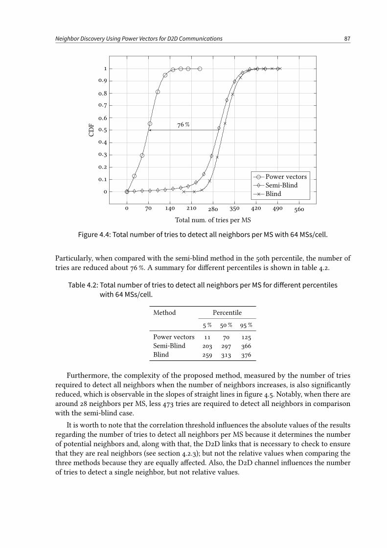
Neighbor Discovery Using Power Vectors for D2D Communications 87
0 70 140 210 280 350 420 490 560
0
0.1
0.2
0.3
0.4
0.5
0.6
0.7
0.8
0.9
1
76 %
Total num. of tries per MS
CDF
Power vectors
Semi-Blind
Blind
Figure 4.4: Total number of tries to detect all neighbors per MS with 64 MSs/cell.
Particularly, when compared with the semi-blind method in the 50th percentile, the number oftries are reduced about 76 %. A summary for dierent percentiles is shown in table 4.2.
Table 4.2: Total number of tries to detect all neighbors per MS for dierent percentiles
with 64 MSs/cell.
Method Percentile
5 % 50% 95%
Power vectors 11 70 125Semi-Blind 203 297 366Blind 259 313 376
Furthermore, the complexity of the proposed method, measured by the number of triesrequired to detect all neighbors when the number of neighbors increases, is also signicantlyreduced, which is observable in the slopes of straight lines in gure 4.5. Notably, when there arearound 28 neighbors per MS, less 473 tries are required to detect all neighbors in comparisonwith the semi-blind case.
It is worth to note that the correlation threshold inuences the absolute values of the resultsregarding the number of tries to detect all neighbors per MS because it determines the numberof potential neighbors and, along with that, the D2D links that is necessary to check to ensurethat they are real neighbors (see section 4.2.3); but not the relative values when comparing thethree methods because they are equally aected. Also, the D2D channel inuences the numberof tries to detect a single neighbor, but not relative values.
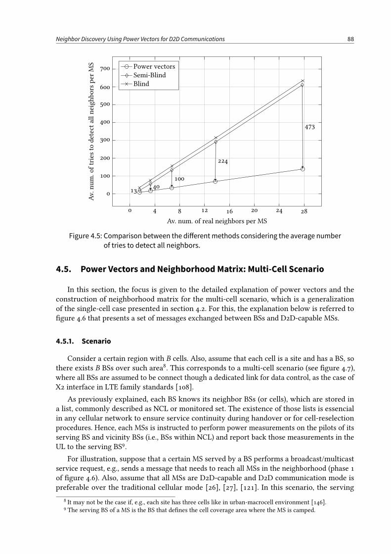
Neighbor Discovery Using Power Vectors for D2D Communications 88
0 4 8 12 16 20 24 28
0
100
200
300
400
500
600
700
1340
100
224
473
Av. num. of real neighbors per MS
Av.num.oftriesto
detectallneighbors
per
MS Power vectors
Semi-Blind
Blind
Figure 4.5: Comparison between the dierentmethods considering the average number
of tries to detect all neighbors.
4.5. Power Vectors and Neighborhood Matrix: Multi-Cell Scenario
In this section, the focus is given to the detailed explanation of power vectors and theconstruction of neighborhood matrix for the multi-cell scenario, which is a generalizationof the single-cell case presented in section 4.2. For this, the explanation below is referred togure 4.6 that presents a set of messages exchanged between BSs and D2D-capable MSs.
4.5.1. Scenario
Consider a certain region with B cells. Also, assume that each cell is a site and has a BS, sothere exists B BSs over such area8. This corresponds to a multi-cell scenario (see gure 4.7),where all BSs are assumed to be connect though a dedicated link for data control, as the case ofX2 interface in LTE family standards [108].
As previously explained, each BS knows its neighbor BSs (or cells), which are stored ina list, commonly described as NCL or monitored set. The existence of those lists is essencialin any cellular network to ensure service continuity during handover or for cell-reselectionprocedures. Hence, each MSs is instructed to perform power measurements on the pilots of itsserving BS and vicinity BSs (i.e., BSs within NCL) and report back those measurements in theUL to the serving BS9.
For illustration, suppose that a certain MS served by a BS performs a broadcast/multicastservice request, e.g., sends a message that needs to reach all MSs in the neighborhood (phase 1of gure 4.6). Also, assume that all MSs are D2D-capable and D2D communication mode ispreferable over the traditional cellular mode [26], [27], [121]. In this scenario, the serving
8 It may not be the case if, e.g., each site has three cells like in urban-macrocell environment [146].9 The serving BS of a MS is the BS that denes the cell coverage area where the MS is camped.
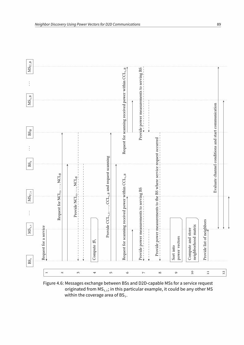
Neighbor Discovery Using Power Vectors for D2D Communications 89BS1
MS1,1
MS U
,1
BS2
BSB
MS1,B
MS U
,B
1 2 3 4 5 6 7 8 9 10 11 12
···
···
···
Requestforaservice
RequestforNCL2,...,NCLB
ProvideNCL2,...,NCLB
ComputeB1
ProvideCCL1,2,...,CCL1,Bandrequestscanning
Requestforscanningreceived
power
within
CCL1,B
Requestforscanningreceived
power
within
CCL1,B
Providepower
measurementsto
servingBS
Providepower
measurementsto
servingBS
Providepower
measurementsto
theBSwhereservicerequestoccurred
Sort
into
power
vectors
Compute
andstore
neighborhoodmatrix
Providelistofneighbors
Evaluatechannelconditionsandstartcommunication
Figure 4.6: Messages exchange between BSs and D2D-capable MSs for a service request
originated from MS1,1; in this particular example, it could be any other MS
within the coverage area of BS1.
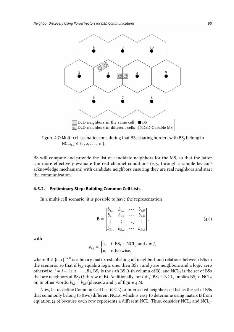
Neighbor Discovery Using Power Vectors for D2D Communications 90
2
34
5
6 7 8
9
10
1
D2D neighbors in the same cell BS
D2D neighbors in dierent cells D2D-Capable MS
Figure 4.7: Multi-cell scenario, considering that BSs sharing borders with BSj belong to
NCLj , j ∈ 1, 2, . . . , 10.
BS will compute and provide the list of candidate neighbors for the MS, so that the lattercan more eectively evaluate the real channel conditions (e.g., through a simple beacon/acknowledge mechanism) with candidate neighbors ensuring they are real neighbors and startthe communication.
4.5.2. Preliminary Step: Building Common Cell Lists
In a multi-cell scenario, it is possible to have the representation
B =
b1,1 b1,2 · · · b1,Bb2,1 b2,2 · · · b2,B...
.... . .
...
bB,1 bB,2 · · · bB,B
, (4.6)
with
bi,j =1, if BSi ∈ NCLj and i , j,
0, otherwise,
where B ∈ 0, 1B×B is a binary matrix establishing all neighborhood relations between BSs inthe scenario, so that if bi,j equals a logic one, then BSs i and j are neighbors and a logic zerootherwise, i , j ∈ 1, 2, . . . ,B, BSi is the i-th BS (i-th column of B), and NCLj is the set of BSsthat are neighbors of BSj (j-th row of B). Additionally, for i , j , BSi ∈ NCLj implies BSj ∈ NCLior, in other words, bi,j = bj,i (phases 2 and 3 of gure 4.6).
Now, let us dene Common Cell List (CCL) or intersected neighbor cell list as the set of BSsthat commonly belong to (two) dierent NCLs; which is easy to determine using matrix B fromequation (4.6) because each row represents a dierent NCL. Thus, consider NCLj and NCLj ′
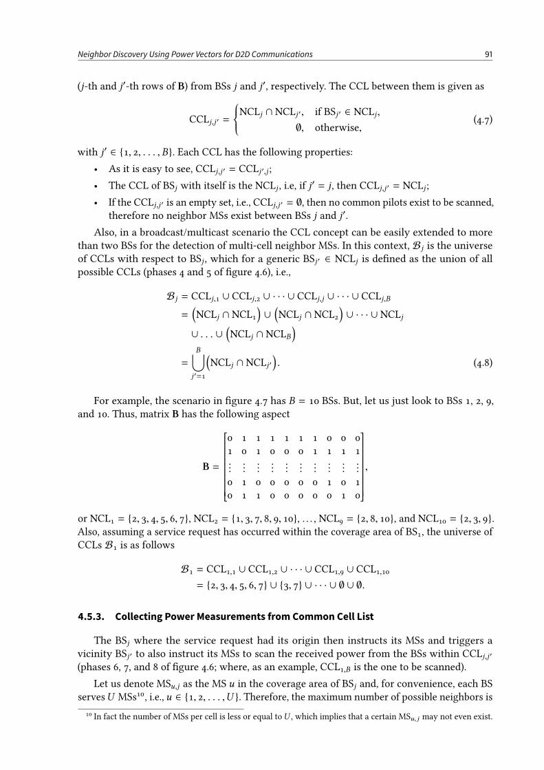
Neighbor Discovery Using Power Vectors for D2D Communications 91
(j-th and j′-th rows of B) from BSs j and j′, respectively. The CCL between them is given as
CCLj,j ′ =NCLj ∩ NCLj ′, if BSj ′ ∈ NCLj ,
∅, otherwise,(4.7)
with j′ ∈ 1, 2, . . . ,B. Each CCL has the following properties:
• As it is easy to see, CCLj,j ′ = CCLj ′,j ;
• The CCL of BSj with itself is the NCLj , i.e, if j′ = j, then CCLj,j ′ = NCLj ;
• If the CCLj,j ′ is an empty set, i.e., CCLj,j ′ = ∅, then no common pilots exist to be scanned,therefore no neighbor MSs exist between BSs j and j′.
Also, in a broadcast/multicast scenario the CCL concept can be easily extended to morethan two BSs for the detection of multi-cell neighbor MSs. In this context, B j is the universeof CCLs with respect to BSj , which for a generic BSj ′ ∈ NCLj is dened as the union of allpossible CCLs (phases 4 and 5 of gure 4.6), i.e.,
B j = CCLj,1 ∪ CCLj,2 ∪ · · · ∪ CCLj,j ∪ · · · ∪ CCLj,B
=
(
NCLj ∩ NCL1)
∪(
NCLj ∩ NCL2)
∪ · · · ∪ NCLj
∪ . . . ∪(
NCLj ∩ NCLB)
=
B⋃
j ′=1
(
NCLj ∩ NCLj ′)
. (4.8)
For example, the scenario in gure 4.7 has B = 10 BSs. But, let us just look to BSs 1, 2, 9,and 10. Thus, matrix B has the following aspect
B =
0 1 1 1 1 1 1 0 0 01 0 1 0 0 0 1 1 1 1..............................
0 1 0 0 0 0 0 1 0 10 1 1 0 0 0 0 0 1 0
,
or NCL1 = 2, 3, 4, 5, 6, 7, NCL2 = 1, 3, 7, 8, 9, 10, . . . , NCL9 = 2, 8, 10, and NCL10 = 2, 3, 9.Also, assuming a service request has occurred within the coverage area of BS1, the universe ofCCLs B1 is as follows
B1 = CCL1,1 ∪ CCL1,2 ∪ · · · ∪ CCL1,9 ∪ CCL1,10= 2, 3, 4, 5, 6, 7 ∪ 3, 7 ∪ · · · ∪ ∅ ∪ ∅.
4.5.3. Collecting Power Measurements from Common Cell List
The BSj where the service request had its origin then instructs its MSs and triggers avicinity BSj ′ to also instruct its MSs to scan the received power from the BSs within CCLj,j ′(phases 6, 7, and 8 of gure 4.6; where, as an example, CCL1,B is the one to be scanned).
Let us denote MSu,j as the MS u in the coverage area of BSj and, for convenience, each BSservesU MSs10, i.e., u ∈ 1, 2, . . . ,U . Therefore, the maximum number of possible neighbors is
10 In fact the number of MSs per cell is less or equal toU , which implies that a certain MSu, j may not even exist.
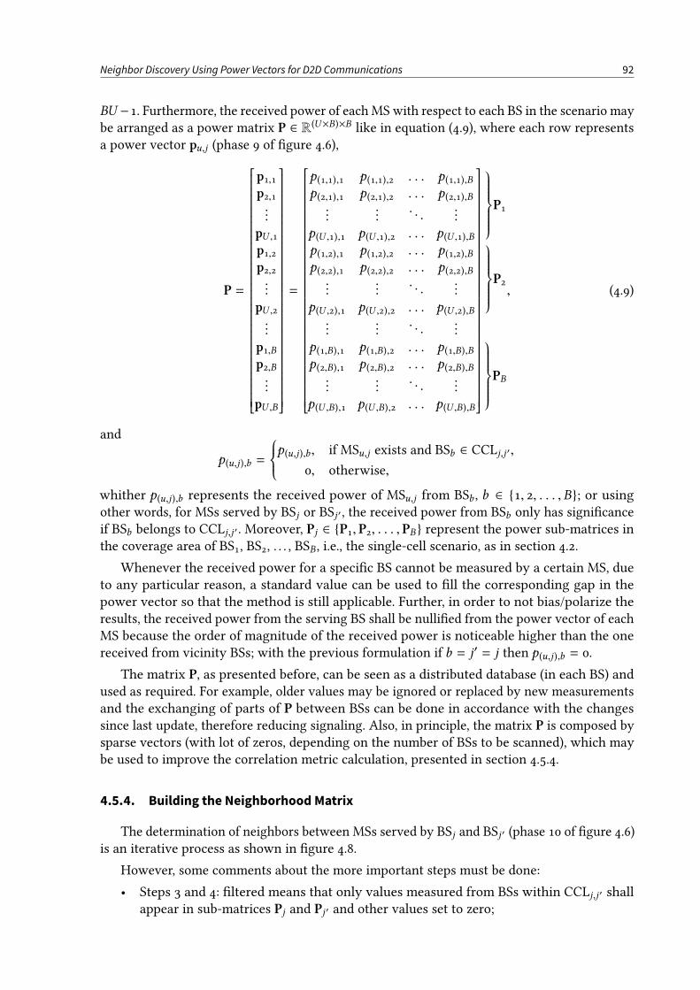
Neighbor Discovery Using Power Vectors for D2D Communications 92
BU −1. Furthermore, the received power of each MS with respect to each BS in the scenario maybe arranged as a power matrix P ∈ R(U×B)×B like in equation (4.9), where each row representsa power vector pu,j (phase 9 of gure 4.6),
P =
p1,1p2,1...
pU ,1p1,2p2,2...
pU ,2...
p1,Bp2,B...
pU ,B
=
p(1,1),1 p(1,1),2 . . . p(1,1),Bp(2,1),1 p(2,1),2 . . . p(2,1),B...
.... . .
...
p(U ,1),1 p(U ,1),2 . . . p(U ,1),Bp(1,2),1 p(1,2),2 . . . p(1,2),Bp(2,2),1 p(2,2),2 . . . p(2,2),B...
.... . .
...
p(U ,2),1 p(U ,2),2 . . . p(U ,2),B...
.... . .
...
p(1,B),1 p(1,B),2 . . . p(1,B),Bp(2,B),1 p(2,B),2 . . . p(2,B),B...
.... . .
...
p(U ,B),1 p(U ,B),2 . . . p(U ,B),B
P1
P2
PB
, (4.9)
and
p(u,j ),b =p(u,j ),b , if MSu,j exists and BSb ∈ CCLj,j ′,
0, otherwise,
whither p(u,j ),b represents the received power of MSu,j from BSb , b ∈ 1, 2, . . . ,B; or usingother words, for MSs served by BSj or BSj ′ , the received power from BSb only has signicanceif BSb belongs to CCLj,j ′ . Moreover, Pj ∈ P1, P2, . . . , PB represent the power sub-matrices inthe coverage area of BS1, BS2, . . . , BSB , i.e., the single-cell scenario, as in section 4.2.
Whenever the received power for a specic BS cannot be measured by a certain MS, dueto any particular reason, a standard value can be used to ll the corresponding gap in thepower vector so that the method is still applicable. Further, in order to not bias/polarize theresults, the received power from the serving BS shall be nullied from the power vector of eachMS because the order of magnitude of the received power is noticeable higher than the onereceived from vicinity BSs; with the previous formulation if b = j′ = j then p(u,j ),b = 0.
The matrix P, as presented before, can be seen as a distributed database (in each BS) andused as required. For example, older values may be ignored or replaced by new measurementsand the exchanging of parts of P between BSs can be done in accordance with the changessince last update, therefore reducing signaling. Also, in principle, the matrix P is composed bysparse vectors (with lot of zeros, depending on the number of BSs to be scanned), which maybe used to improve the correlation metric calculation, presented in section 4.5.4.
4.5.4. Building the Neighborhood Matrix
The determination of neighbors between MSs served by BSj and BSj ′ (phase 10 of gure 4.6)is an iterative process as shown in gure 4.8.
However, some comments about the more important steps must be done:
• Steps 3 and 4: ltered means that only values measured from BSs within CCLj,j ′ shallappear in sub-matrices Pj and Pj ′ and other values set to zero;
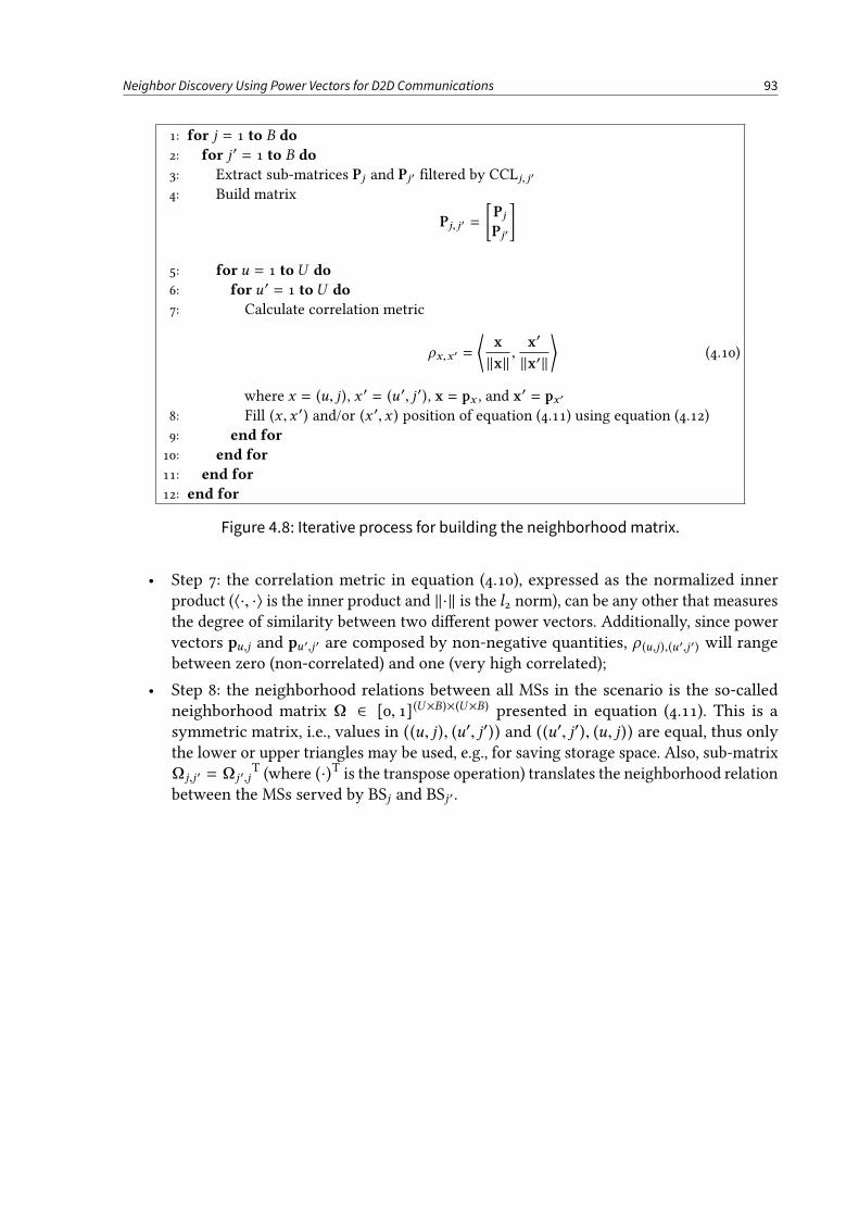
Neighbor Discovery Using Power Vectors for D2D Communications 93
1: for j = 1 to B do2: for j ′ = 1 to B do3: Extract sub-matrices Pj and Pj′ ltered by CCLj, j′4: Build matrix
Pj, j′ =
[PjPj′
]
5: for u = 1 toU do6: for u ′ = 1 toU do7: Calculate correlation metric
ρx,x ′ =
⟨
x
‖x‖,
x′
‖x′‖
⟩
(4.10)
where x = (u, j ), x ′ = (u ′, j ′), x = px , and x′ = px ′
8: Fill (x ,x ′) and/or (x ′,x ) position of equation (4.11) using equation (4.12)9: end for10: end for11: end for12: end for
Figure 4.8: Iterative process for building the neighborhoodmatrix.
• Step 7: the correlation metric in equation (4.10), expressed as the normalized innerproduct (〈·, ·〉 is the inner product and ‖·‖ is the l2 norm), can be any other that measuresthe degree of similarity between two dierent power vectors. Additionally, since powervectors pu,j and pu ′,j ′ are composed by non-negative quantities, ρ (u,j ),(u ′,j ′) will rangebetween zero (non-correlated) and one (very high correlated);
• Step 8: the neighborhood relations between all MSs in the scenario is the so-calledneighborhood matrix Ω ∈ [0, 1](U×B)×(U×B) presented in equation (4.11). This is asymmetric matrix, i.e., values in ((u, j ), (u′, j′)) and ((u′, j′), (u, j )) are equal, thus onlythe lower or upper triangles may be used, e.g., for saving storage space. Also, sub-matrixΩj,j ′ = Ωj ′,j
T (where (·)T is the transpose operation) translates the neighborhood relationbetween the MSs served by BSj and BSj ′ .
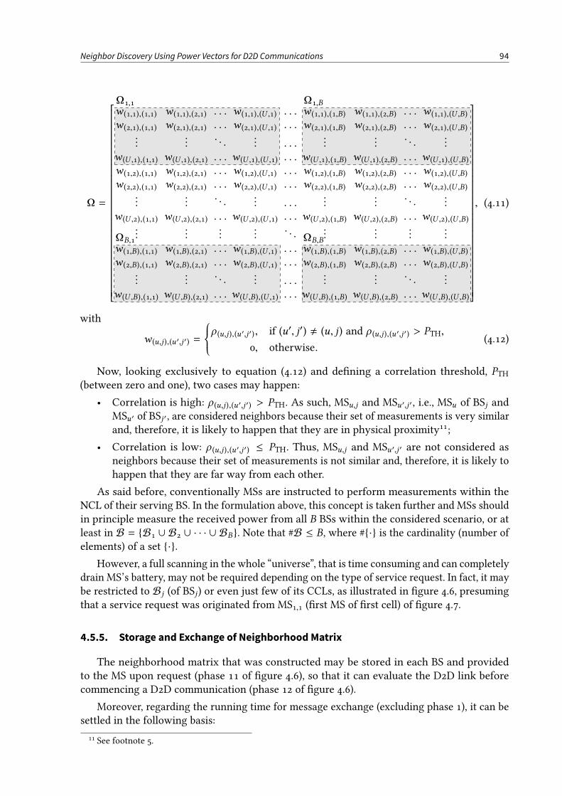
Neighbor Discovery Using Power Vectors for D2D Communications 94
Ω1,1 Ω1,B
ΩB,1 ΩB,B
Ω =
w (1,1),(1,1) w (1,1),(2,1) . . . w (1,1),(U ,1) . . . w (1,1),(1,B) w (1,1),(2,B) . . . w (1,1),(U ,B)
w (2,1),(1,1) w (2,1),(2,1) . . . w (2,1),(U ,1) . . . w (2,1),(1,B) w (2,1),(2,B) . . . w (2,1),(U ,B)...
.... . .
... . . ....
.... . .
...
w (U ,1),(1,1) w (U ,1),(2,1) . . . w (U ,1),(U ,1) . . . w (U ,1),(1,B) w (U ,1),(2,B) . . . w (U ,1),(U ,B)
w (1,2),(1,1) w (1,2),(2,1) . . . w (1,2),(U ,1) . . . w (1,2),(1,B) w (1,2),(2,B) . . . w (1,2),(U ,B)
w (2,2),(1,1) w (2,2),(2,1) . . . w (2,2),(U ,1) . . . w (2,2),(1,B) w (2,2),(2,B) . . . w (2,2),(U ,B)...
.... . .
... . . ....
.... . .
...
w (U ,2),(1,1) w (U ,2),(2,1) . . . w (U ,2),(U ,1) . . . w (U ,2),(1,B) w (U ,2),(2,B) . . . w (U ,2),(U ,B)...
......
.... . .
......
......
w (1,B),(1,1) w (1,B),(2,1) . . . w (1,B),(U ,1) . . . w (1,B),(1,B) w (1,B),(2,B) . . . w (1,B),(U ,B)
w (2,B),(1,1) w (2,B),(2,1) . . . w (2,B),(U ,1) . . . w (2,B),(1,B) w (2,B),(2,B) . . . w (2,B),(U ,B)...
.... . .
... . . ....
.... . .
...
w (U ,B),(1,1) w (U ,B),(2,1) . . . w (U ,B),(U ,1) . . . w (U ,B),(1,B) w (U ,B),(2,B) . . . w (U ,B),(U ,B)
, (4.11)
with
w (u,j ),(u ′,j ′) =
ρ (u,j ),(u ′,j ′), if (u′, j′) , (u, j ) and ρ (u,j ),(u ′,j ′) > PTH,
0, otherwise.(4.12)
Now, looking exclusively to equation (4.12) and dening a correlation threshold, PTH(between zero and one), two cases may happen:
• Correlation is high: ρ (u,j ),(u ′,j ′) > PTH. As such, MSu,j and MSu ′,j ′, i.e., MSu of BSj andMSu ′ of BSj ′ , are considered neighbors because their set of measurements is very similarand, therefore, it is likely to happen that they are in physical proximity11;
• Correlation is low: ρ (u,j ),(u ′,j ′) ≤ PTH. Thus, MSu,j and MSu ′,j ′ are not considered asneighbors because their set of measurements is not similar and, therefore, it is likely tohappen that they are far way from each other.
As said before, conventionally MSs are instructed to perform measurements within theNCL of their serving BS. In the formulation above, this concept is taken further and MSs shouldin principle measure the received power from all B BSs within the considered scenario, or atleast in B = B1 ∪ B2 ∪ · · · ∪ BB . Note that #B ≤ B, where #· is the cardinality (number ofelements) of a set ·.
However, a full scanning in the whole “universe”, that is time consuming and can completelydrain MS’s battery, may not be required depending on the type of service request. In fact, it maybe restricted to B j (of BSj) or even just few of its CCLs, as illustrated in gure 4.6, presumingthat a service request was originated from MS1,1 (rst MS of rst cell) of gure 4.7.
4.5.5. Storage and Exchange of Neighborhood Matrix
The neighborhood matrix that was constructed may be stored in each BS and providedto the MS upon request (phase 11 of gure 4.6), so that it can evaluate the D2D link beforecommencing a D2D communication (phase 12 of gure 4.6).
Moreover, regarding the running time for message exchange (excluding phase 1), it can besettled in the following basis:
11 See footnote 5.
Neighbor Discovery Using Power Vectors for D2D Communications 95
• Phases 2 to 8: may be done at every 200ms to 1 s, or 200 to 1000 TTIs [143];
• Phases 9 to 12: may be done at each new service request or whenever theMS is scheduled.
4.6. Conclusion
In this chapter we proposed and explained a neighbor discovery process based on powervectors for network-assisted D2D communications. The method may be used in current wirelesssystems because it uses the already available measurements and does not add considerablenetwork load on signaling. First the method was presented for a single-cell scenario and latterextended for the multi-cell case.
In the single-cell scenario, results show that with the network help, the time to detect allneighbors per MS is signicantly reduced, letting more time for data transmission. For themulti-cell case results are not expected to change much. Nevertheless, the eort to computethe neighborhood matrix tends to increase as the number of BSs increases, which is likely tohappen in a Fifth Generation (5G) scenario with network densication, especially the spatialdensication [150]. On the other side, if the number of BSs (i.e., the cardinality of a CCL betweentwo BSs) is low, the quality of the cross correlation metric can be compromised.
The proposed method is able to operate in Frequency Division Duplex (FDD) and TimeDivision Duplex (TDD) modes and is not dependent on the radio access technology. Moreover,and especially, it overcomes the problems presented in section 4.1.2, in the following manner:
• Time to discover and stopping criteria: given that a set of neighbors is built at the BS,the number of MS neighbors becomes known and, therefore, the time to discover isjust the time to evaluate the real channel conditions for the D2D links of the candidateneighbors, as well as the stopping criteria, i.e., the criteria that sets when the discoveryprocess shall stop, can be better dened/adjusted;
• Power management: the MS power that is consumed in the discovery process is lowerbecause the main work is done at the BS, building the neighborhood relations, which foreach MS is considered to be a small set. Thus, just before the session establishment, theMS just needs to ensure that D2D communication can be established through the directchannel, which can be done, e.g., by a single pair of beacon/acknowledgement packets;
• New protocol implementation: no new protocol is required to be implemented forthe measurement process because signal quality measurements are already available/exchanged in the network and are mandatory for it to operate. Also, BSs are connectedthough a dedicated link for data control, so no new link is required. However, three newtypes of messages will be required: for exchanging the NCL lists between BSs; for therange of BSs to be scanned; and for each BS to inform the neighbor candidate list toeach MS;
• Hidden MS problem: this problemwill simply not exist. Building the neighborhood matrixis a centralized process and since the BS is aware of any D2D direct communicationthat is ongoing, if any candidate neighbor is potentially seen as “hidden”, it may be justremoved from the neighborhood matrix, therefore avoiding the problem;
• The multi-cell cases, i.e., MSs that belong to dierent cells (served by dierent BSs) areable to discover each other, enabling the cross-cell border D2D communications;
• The NCL of each BSmay be especially large, e.g., in crowded areas where the deploymentis based on small cells. With the introduction of CCL concept, the number of BSs to

Neighbor Discovery Using Power Vectors for D2D Communications 96
be scanned for each MS is limited, which reduces the power wasted in the scanning,therefore improving the MS’ batteries lifetime.
Finally, future works on this topic may focus on:
• Simulate the discovery of MSs that belong to dierent cells (served by dierent BSs),which may happen close to cell boundaries;
• Implement a timeout for the discover to happen (detection window) and count thefalse/missed detections;
• Discover neighbors that do not fulll the service request, which can be especially usefulin social networks;
• Evaluate the proposed method based on power vectors in real celular networks underlaidby D2D communications.
CHAPTER 5
Band Selection for D2D Communications
For systems with reuse factor less than one, the co-channel interference can drasticallyreduce the gain of primary networks, which limits the whole system performance. This
chapter exploits the selection of Downlink (DL) or Uplink (UL) band to be reused by a Device-to-Device (D2D) link. The band selected by the method is based on a radio distance metric, suchas received power. Despite being a simple concept, results have shown that band selection caneectively mitigate the interference caused by D2D communications in a Long Term Evolution(LTE) network. Therefore, the coexistence of cellular and D2D communication modes becomespossible in time, frequency, and space.
5.1. Introduction
As mentioned in chapter 1, D2D communication is a type of direct wireless communicationbetween two or more network nodes, hereafter generally referred as User Equipments (UEs),similar to direct-mode operation in professional mobile radio systems or the bluetooth technol-ogy, that has attracted increasing attention of the scientic community in the last couple ofyears, mostly because of its exibility [26]: D2D communications can be deployed in Industrial,Scientic and Medical (ISM) bands for the unlicensed spectrum use, such as Wireless LocalArea Networks (WLANs), or in cellular networks for a licensed use [27].
D2D communications are particularly attractive considering the reuse gain obtained whenD2D-capable UEs are allowed to directly transmit data by reusing either DL or UL radioresources from the cellular network [32]. However, operating in the in-band shared spectrummode [44], secondary D2D communications pose new challenging interference situations, suchas the co-channel interference, due to orthogonality loss [33], which can drastically reduce theperformance of primary cellular communications [52].
Some of the already studied solutions to deal with this problem and improve the overallnetwork throughput include, e.g., power control, spatial diversity, robust centralized/distributedresource allocation, mode selection and grouping, or network coding [32], [44] (recall gure 1.4).In this chapter we investigate the interference mitigation by using an intelligent selection ofthe transmission band, either DL or UL, for the D2D link when sharing spectrum resourceswith an LTE network. Nevertheless, the method is still valid for a time-based duplexing schemeand other types of wireless systems. Also, dierently from most of state of the art publicationsthat focus on interference mitigation, herein we consider a realistic multi-user/cell scenario,with wrap-around, and both communication directions.
The remaining sections of this chapter are organized as follows: in section 5.2 the principlebehind band selection technique is presented and explained in detail, section 5.3 has the
97
Band Selection for D2D Communications 98
description of system models used for simulations, in section 5.4 the principal results are shownand analyzed, lastly conclusions are drawn in section 5.5.
5.2. Band Selection
5.2.1. Overview
The main principle behind band selection for interference mitigation is to either select DLor UL band for the D2D link using a radio distance metric, like the received power, pr . Thedecision-taking procedure veries if the received power from the serving Evolved Node B (eNB)of the transmitter within the D2D pair1 is above a given threshold, PrTH, and if it yields true,the DL band is selected; otherwise, the UL band is used, as presented in gure 5.1.
The pr is measured from the serving eNB (eNB-UE link), not within the D2D pair (UE-UElink), and attempts tomap the position of the interferer (D2D-capable UE that acts as transmitter)within the cell, since the real location is most of the times unavailable (see gure 5.2). Thehigher is the received power, the lower is the distance to eNB. Thus, above threshold means“near eNB”, while below the threshold translates “at cell-edge” position (see gure 5.3).
Furthermore, the method must be applied for all D2D pairs in each Transmission TimeInterval (TTI) because of channel variations. Also, we refer as active pairs the ones with thesame selected band as the current communication phase, i.e., reuse DL band in DL phase orreuse UL band in the UL phase.
For LTE networks, the band selection technique is performed per Physical Resource Block(PRB) and also includes the grouping of one active pair (selected randomly or by any othermean) with the primary scheduled cellular UE to either reuse the DL or UL PRBs (see gure 5.5).In this situation, system-specic measurements like Reference Signal Received Power (RSRP),Received Signal Strength Indicator (RSSI), or even Reference Signal Received Quality (RSRQ)may be used alone or combined to be the radio distance metric.
5.2.2. The Underlaying Concept
Consider the picture in gure 5.2, where h and д denote the complex channel coecients,respectively associated with desired and interfering gains. These channels are assumed tobe asymmetric, i.e., DL and UL channels may have dierent gains. The simplied scenariorepresented therein also suers outside interference from the surrounding cells that are usingthe same PRB. That interference channel can be generally designated as ik , where k refers to theindex of the interferer Ik (eNB or UE). Also, each receiver is subject to experience additive whiteGaussian noise n3,n4 ∼ CN (0,σ 2). Moreover, the transmitted data symbols are representedas x , and we assume that |x1 |2 = |x3 |2 = |x4 |2 = |xIk |2 = 1. Thereby, the received signals at
1 A pair formed by two D2D-capable UEs (transmitter and receiver) that use the direct path to communicate.
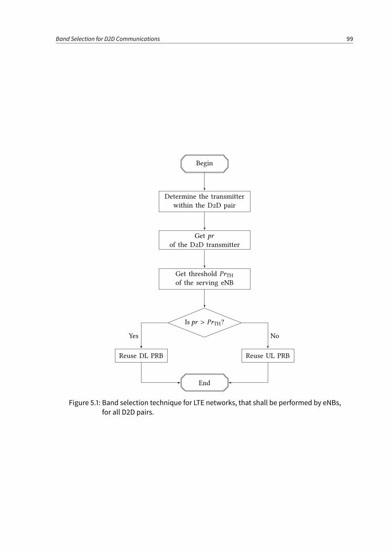
Band Selection for D2D Communications 99
Begin
Determine the transmitter
within the D2D pair
Get pr
of the D2D transmitter
Get threshold PrTHof the serving eNB
Is pr > PrTH?
Reuse DL PRB Reuse UL PRB
End
Yes No
Figure 5.1: Band selection technique for LTE networks, that shall be performed by eNBs,
for all D2D pairs.
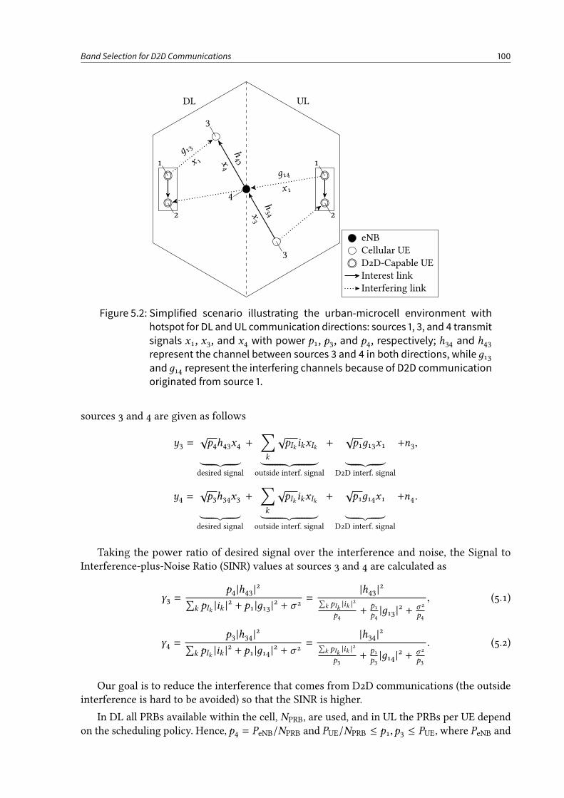
Band Selection for D2D Communications 100
3
3
4
1 1
2 2
DL UL
h43x
4
h34x
3
д 13
x 1
д14
x1
eNB
Cellular UE
D2D-Capable UE
Interest link
Interfering link
Figure 5.2: Simplified scenario illustrating the urban-microcell environment with
hotspot for DL and UL communication directions: sources 1, 3, and 4 transmit
signals x1, x3, and x4 with power p1, p3, and p4, respectively; h34 and h43represent the channel between sources 3 and 4 in both directions, whileд13andд14 represent the interfering channels because of D2D communication
originated from source 1.
sources 3 and 4 are given as follows
y3 =√p4h43x4
︸ ︷︷ ︸desired signal
+
∑
k
√pIk ikxIk
︸ ︷︷ ︸outside interf. signal
+
√p1д13x1
︸ ︷︷ ︸D2D interf. signal
+n3,
y4 =√p3h34x3
︸ ︷︷ ︸desired signal
+
∑
k
√pIk ikxIk
︸ ︷︷ ︸outside interf. signal
+
√p1д14x1
︸ ︷︷ ︸D2D interf. signal
+n4.
Taking the power ratio of desired signal over the interference and noise, the Signal toInterference-plus-Noise Ratio (SINR) values at sources 3 and 4 are calculated as
γ3 =p4 |h43 |2
∑
k pIk |ik |2 + p1 |д13 |2 + σ 2=
|h43 |2∑
k pIk |ik |2
p4+
p1p4|д13 |2 + σ 2
p4
, (5.1)
γ4 =p3 |h34 |2
∑
k pIk |ik |2 + p1 |д14 |2 + σ 2=
|h34 |2∑
k pIk |ik |2
p3+
p1p3|д14 |2 + σ 2
p3
. (5.2)
Our goal is to reduce the interference that comes from D2D communications (the outsideinterference is hard to be avoided) so that the SINR is higher.
In DL all PRBs available within the cell, NPRB, are used, and in UL the PRBs per UE dependon the scheduling policy. Hence, p4 = PeNB/NPRB and PUE/NPRB ≤ p1,p3 ≤ PUE, where PeNB and
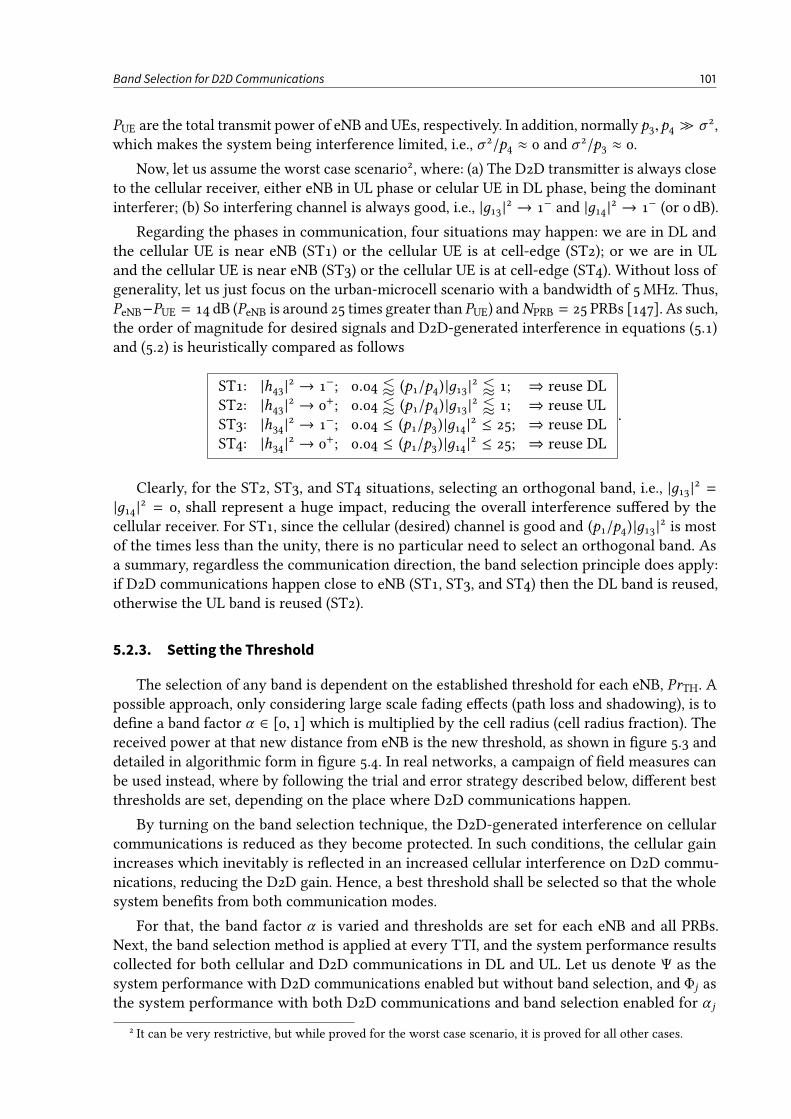
Band Selection for D2D Communications 101
PUE are the total transmit power of eNB and UEs, respectively. In addition, normally p3,p4 ≫ σ 2,which makes the system being interference limited, i.e., σ 2/p4 ≈ 0 and σ 2/p3 ≈ 0.
Now, let us assume the worst case scenario2, where: (a) The D2D transmitter is always closeto the cellular receiver, either eNB in UL phase or celular UE in DL phase, being the dominantinterferer; (b) So interfering channel is always good, i.e., |д13 |2 → 1− and |д14 |2 → 1− (or 0 dB).
Regarding the phases in communication, four situations may happen: we are in DL andthe cellular UE is near eNB (ST1) or the cellular UE is at cell-edge (ST2); or we are in ULand the cellular UE is near eNB (ST3) or the cellular UE is at cell-edge (ST4). Without loss ofgenerality, let us just focus on the urban-microcell scenario with a bandwidth of 5MHz. Thus,PeNB−PUE = 14 dB (PeNB is around 25 times greater than PUE) andNPRB = 25 PRBs [147]. As such,the order of magnitude for desired signals and D2D-generated interference in equations (5.1)and (5.2) is heuristically compared as follows
ST1: |h43 |2 → 1−; 0.04 / (p1/p4) |д13 |2 / 1; ⇒ reuse DLST2: |h43 |2 → 0+; 0.04 / (p1/p4) |д13 |2 / 1; ⇒ reuse ULST3: |h34 |2 → 1−; 0.04 ≤ (p1/p3) |д14 |2 ≤ 25; ⇒ reuse DLST4: |h34 |2 → 0+; 0.04 ≤ (p1/p3) |д14 |2 ≤ 25; ⇒ reuse DL
.
Clearly, for the ST2, ST3, and ST4 situations, selecting an orthogonal band, i.e., |д13 |2 =|д14 |2 = 0, shall represent a huge impact, reducing the overall interference suered by thecellular receiver. For ST1, since the cellular (desired) channel is good and (p1/p4) |д13 |2 is mostof the times less than the unity, there is no particular need to select an orthogonal band. Asa summary, regardless the communication direction, the band selection principle does apply:if D2D communications happen close to eNB (ST1, ST3, and ST4) then the DL band is reused,otherwise the UL band is reused (ST2).
5.2.3. Setting the Threshold
The selection of any band is dependent on the established threshold for each eNB, PrTH. Apossible approach, only considering large scale fading eects (path loss and shadowing), is todene a band factor α ∈ [0, 1] which is multiplied by the cell radius (cell radius fraction). Thereceived power at that new distance from eNB is the new threshold, as shown in gure 5.3 anddetailed in algorithmic form in gure 5.4. In real networks, a campaign of eld measures canbe used instead, where by following the trial and error strategy described below, dierent bestthresholds are set, depending on the place where D2D communications happen.
By turning on the band selection technique, the D2D-generated interference on cellularcommunications is reduced as they become protected. In such conditions, the cellular gainincreases which inevitably is reected in an increased cellular interference on D2D commu-nications, reducing the D2D gain. Hence, a best threshold shall be selected so that the wholesystem benets from both communication modes.
For that, the band factor α is varied and thresholds are set for each eNB and all PRBs.Next, the band selection method is applied at every TTI, and the system performance resultscollected for both cellular and D2D communications in DL and UL. Let us denote Ψ as thesystem performance with D2D communications enabled but without band selection, and Φj asthe system performance with both D2D communications and band selection enabled for α j
2 It can be very restrictive, but while proved for the worst case scenario, it is proved for all other cases.
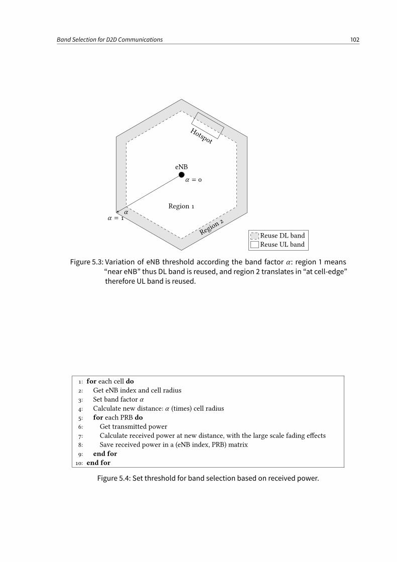
Band Selection for D2D Communications 102
Region 1
Regio
n 2
α = 0
α = 1α
eNB
Hotspot
Reuse DL band
Reuse UL band
Figure 5.3: Variation of eNB threshold according the band factor α : region 1 means
“near eNB” thus DL band is reused, and region 2 translates in “at cell-edge”
therefore UL band is reused.
1: for each cell do2: Get eNB index and cell radius3: Set band factor α4: Calculate new distance: α (times) cell radius5: for each PRB do6: Get transmitted power7: Calculate received power at new distance, with the large scale fading eects8: Save received power in a (eNB index, PRB) matrix9: end for10: end for
Figure 5.4: Set threshold for band selection based on received power.
Band Selection for D2D Communications 103
(the communication direction and mode were omitted in the notation for simplicity). So thebest band factor α⋆ is obtained as follows
α⋆ = argmaxj
(Cj
Dj
)
,∀α j , (5.3)
where, for α j ,
Cj = max(
|Ψ − Φj |DL, |Ψ − Φj |UL)
cell, (5.4)
Dj = max(
|Ψ − Φj |DL, |Ψ − Φj |UL)
D2D, (5.5)
andA = 0, 0.1, . . . , 1 and j = 1, 2, . . . , #A and α j ∈ A.
In the case of cellular communications we desire to maximize Cj (equation (5.4)), i.e., nd(Φj )cell ≫ Ψcell, because on such situation the gain provided by cellular communications ismaximum in the presence of D2D communications. On the other hand, when band selection isnot enabled, the gain of D2D communications is maximum, but they have strong impact oncellular communications; thus maximizing Dj (equation (5.5)), i.e., nding (Φj )D2D ≪ ΨD2D, isthe same as minimizing the D2D gain or the generated interference. The best trade-o betweensystem performance and interference mitigation is then ensured by maximizing the ratioCj/Dj ,as presented in equation (5.3).
5.3. SystemModel and Simulation Framework
In previous sections a simplied signal model was used. In this one, realistic models thatwere employed to evaluate the system performance are described. Hence, consider an LTE-likenetwork based on the urban-microcell propagation environment, where each eNB is placed inthe center of a site (a single-cell) represented regular hexagon [146]. This scenario correspondsto a multi-cell network with Ncell cells regularly distributed over it and each cell serves NUE
UEs.
Also, there is a hotspot per cell where D2D communications happen. A percentage of thetotal number of UEs within the cell is clustered inside the hotspot zone while the remainingUEs are uniformly distributed over the cell area. Moreover, the D2D pairs are obtained bya simple random pairing of UEs inside the hotspot. However, in our model, UEs within thehotspot may be chosen by the scheduling policy at each TTI, therefore acting as cellular UEs.gure 5.2 exemplies both cellular and D2D communications.
The modeling of complex channel coecients follow a PRB basis, including the propagationeects on wireless channels, namely, pathloss, shadowing, and fast fading [146], [147], [151].Additionally, we consider a number ofNPRB PRBs available in each link direction (determined bythe system bandwidth) that can be fully reused by all cells. Furthermore, the channel responsefor each PRB is represented by the complex channel coecient associated with its middlesubcarrier and rst Orthogonal Frequency Division Multiplexing (OFDM) symbol; and thechannel coherence bandwidth is assumed to be larger than the bandwidth of a PRB, leading toa at fading channel over each of them.
Due to practical reasons, subcarriers are grouped in blocks of 12 adjacent subcarriers spacedby 15 kHz, which gives a total bandwidth of 180 kHz per block. At each TTI or 1ms, information
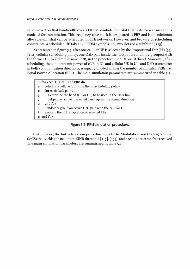
Band Selection for D2D Communications 104
is conveyed on that bandwidth over 7 OFDM symbols (one slot that lasts for 0.50ms) and ismodeled for transmission. This frequency-time block is designated as PRB and is the minimumallocable unit that can be scheduled in LTE networks. However, and because of schedulingconstraints, a scheduled UE takes 14 OFDM symbols, i.e., two slots or a subframe [115].
As presented in gure 5.5, after one cellular UE is selected by the Proportional Fair (PF) [53],[152] cellular scheduling policy, one D2D pair inside the hotspot is randomly grouped withthe former UE to share the same PRB, in the predetermined DL or UL band. Moreover, afterscheduling, the total transmit power of eNB in DL and cellular UE in UL, and D2D transmitterin both communication directions, is equally divided among the number of allocated PRBs, i.e.,Equal Power Allocation (EPA). The main simulation parameters are summarized in table 5.1.
1: for each TTI, cell, and PRB do2: Select one cellular UE using the PF scheduling policy3: for each D2D pair do4: Determine the band (DL or UL) to be used in the D2D link5: Set pair as active if selected band equals the comm. direction6: end for7: Randomly group an active D2D pair with the cellular UE8: Perform the link adaptation of selected UEs9: end for
Figure 5.5: RRM simulation procedure.
Furthermore, the link adaptation procedure selects the Modulation and Coding Scheme(MCS) that yields the maximum SINR threshold [115], [153], and packets are error-free received.The main simulation parameters are summarized in table 5.1.
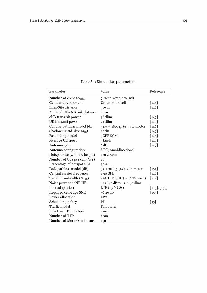
Band Selection for D2D Communications 105
Table 5.1: Simulation parameters.
Parameter Value Reference
Number of eNBs (Ncell) 7 (with wrap-around)Cellular environment Urban-microcell [146]Inter-Site distance 500m [146]Minimal UE-eNB link distance 20meNB transmit power 38 dBm [147]UE transmit power 24 dBm [147]Cellular pathloss model [dB] 34.5 + 38 log10 (d ), d in meter [146]Shadowing std. dev. (σsh) 10 dB [147]Fast fading model 3GPP SCM [146]Average UE speed 3 km/h [147]Antenna gain 6 dBi [147]Antenna conguration SISO, omnidirectionalHotspot size (width × height) 120 × 50mNumber of UEs per cell (NUE) 16Percentage of hotspot UEs 50 %D2D pathloss model [dB] 37 + 30 log10 (d ), d in meter [151]Central carrier frequency 1.90GHz [146]System bandwidth (NPRB) 5MHz DL/UL (25 PRBs each) [114]Noise power at eNB/UE −116.40 dBm/−112.40 dBmLink adaptation LTE (15 MCSs) [115], [153]Required cell-edge SNR −6.20 dB [153]Power allocation EPAScheduling policy PF [53]Trac model Full buerEective TTI duration 1msNumber of TTIs 1000Number of Monte Carlo runs 150
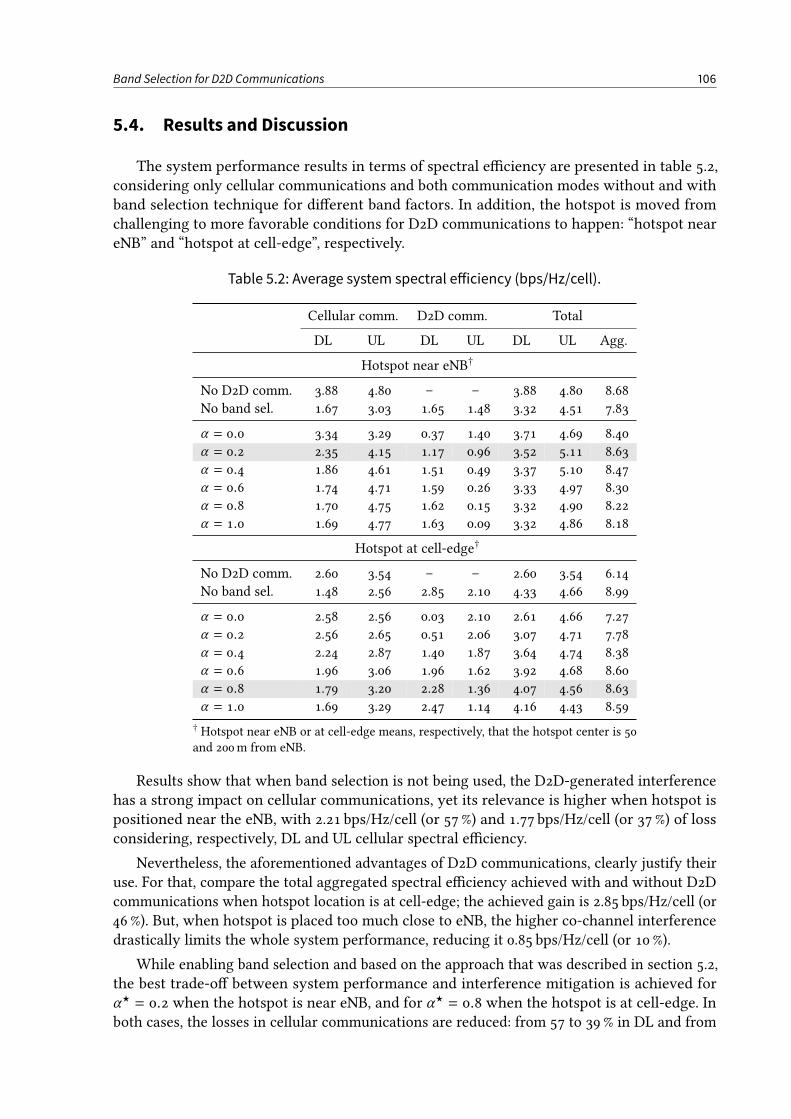
Band Selection for D2D Communications 106
5.4. Results and Discussion
The system performance results in terms of spectral eciency are presented in table 5.2,considering only cellular communications and both communication modes without and withband selection technique for dierent band factors. In addition, the hotspot is moved fromchallenging to more favorable conditions for D2D communications to happen: “hotspot neareNB” and “hotspot at cell-edge”, respectively.
Table 5.2: Average system spectral eiciency (bps/Hz/cell).
Cellular comm. D2D comm. Total
DL UL DL UL DL UL Agg.
Hotspot near eNB†
No D2D comm. 3.88 4.80 – – 3.88 4.80 8.68No band sel. 1.67 3.03 1.65 1.48 3.32 4.51 7.83
α = 0.0 3.34 3.29 0.37 1.40 3.71 4.69 8.40α = 0.2 2.35 4.15 1.17 0.96 3.52 5.11 8.63α = 0.4 1.86 4.61 1.51 0.49 3.37 5.10 8.47α = 0.6 1.74 4.71 1.59 0.26 3.33 4.97 8.30α = 0.8 1.70 4.75 1.62 0.15 3.32 4.90 8.22α = 1.0 1.69 4.77 1.63 0.09 3.32 4.86 8.18
Hotspot at cell-edge†
No D2D comm. 2.60 3.54 – – 2.60 3.54 6.14No band sel. 1.48 2.56 2.85 2.10 4.33 4.66 8.99
α = 0.0 2.58 2.56 0.03 2.10 2.61 4.66 7.27α = 0.2 2.56 2.65 0.51 2.06 3.07 4.71 7.78α = 0.4 2.24 2.87 1.40 1.87 3.64 4.74 8.38α = 0.6 1.96 3.06 1.96 1.62 3.92 4.68 8.60α = 0.8 1.79 3.20 2.28 1.36 4.07 4.56 8.63α = 1.0 1.69 3.29 2.47 1.14 4.16 4.43 8.59
† Hotspot near eNB or at cell-edge means, respectively, that the hotspot center is 50and 200m from eNB.
Results show that when band selection is not being used, the D2D-generated interferencehas a strong impact on cellular communications, yet its relevance is higher when hotspot ispositioned near the eNB, with 2.21 bps/Hz/cell (or 57 %) and 1.77 bps/Hz/cell (or 37 %) of lossconsidering, respectively, DL and UL cellular spectral eciency.
Nevertheless, the aforementioned advantages of D2D communications, clearly justify theiruse. For that, compare the total aggregated spectral eciency achieved with and without D2Dcommunications when hotspot location is at cell-edge; the achieved gain is 2.85 bps/Hz/cell (or46 %). But, when hotspot is placed too much close to eNB, the higher co-channel interferencedrastically limits the whole system performance, reducing it 0.85 bps/Hz/cell (or 10 %).
While enabling band selection and based on the approach that was described in section 5.2,the best trade-o between system performance and interference mitigation is achieved forα⋆ = 0.2 when the hotspot is near eNB, and for α⋆ = 0.8 when the hotspot is at cell-edge. Inboth cases, the losses in cellular communications are reduced: from 57 to 39 % in DL and from
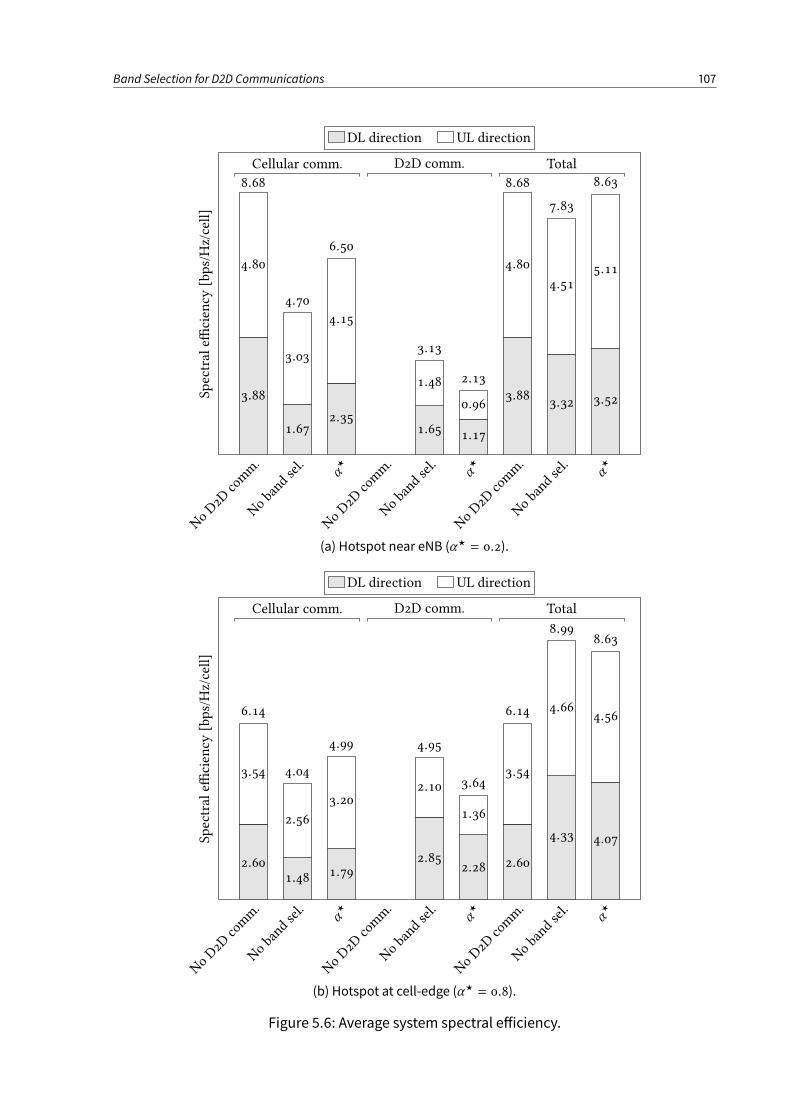
Band Selection for D2D Communications 107
NoD2D
comm.
Nobandsel.
α
⋆
NoD2D
comm.
Nobandsel.
α
⋆
NoD2D
comm.
Nobandsel.
α
⋆
4.80
8.68
3.03
4.70
4.15
6.50
1.48
3.13
0.96
2.13
4.80
8.68
4.51
7.83
5.11
8.63
3.88
1.672.35
1.65 1.17
3.883.32 3.52
Cellular comm. D2D comm. Total
Spectrale
ciency
[bps/Hz/cell]
DL direction UL direction
(a) Hotspot near eNB (α⋆= 0.2).
NoD2D
comm.
Nobandsel.
α
⋆
NoD2D
comm.
Nobandsel.
α
⋆
NoD2D
comm.
Nobandsel.
α
⋆
3.54
6.14
2.56
4.04
3.20
4.99
2.10
4.95
1.36
3.643.54
6.14 4.66
8.99
4.56
8.63
2.601.48 1.79
2.852.28 2.60
4.33 4.07
Cellular comm. D2D comm. Total
Spectrale
ciency
[bps/Hz/cell]
DL direction UL direction
(b) Hotspot at cell-edge (α⋆= 0.8).
Figure 5.6: Average system spectral eiciency.
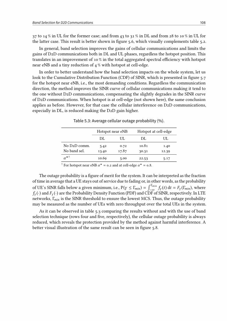
Band Selection for D2D Communications 108
37 to 14 % in UL for the former case; and from 43 to 31 % in DL and from 28 to 10 % in UL forthe latter case. This result is better shown in gure 5.6, which visually complements table 5.2.
In general, band selection improves the gains of cellular communications and limits thegains of D2D communications both in DL and UL phases, regardless the hotspot position. Thistranslates in an improvement of 10 % in the total aggregated spectral eciency with hotspotnear eNB and a tiny reduction of 4 % with hotspot at cell-edge.
In order to better understand how the band selection impacts on the whole system, let uslook to the Cumulative Distribution Function (CDF) of SINR, which is presented in gure 5.7for the hotspot near eNB, i.e., the most demanding conditions. Regardless the communicationdirection, the method improves the SINR curve of cellular communications making it tend tothe one without D2D communications, compensating the slightly degrades in the SINR curveof D2D communications. When hotspot is at cell-edge (not shown here), the same conclusionapplies as before. However, for that case the cellular interference on D2D communications,especially in DL, is reduced making the D2D gain higher.
Table 5.3: Average cellular outage probability (%).
Hotspot near eNB Hotspot at cell-edge
DL UL DL UL
No D2D comm. 5.42 0.72 10.81 1.40No band sel. 13.40 17.87 30.31 12.39
α⋆† 10.69 5.00 22.53 5.17
† For hotspot near eNB α⋆= 0.2 and at cell-edge α⋆
= 0.8.
The outage probability is a gure of merit for the system. It can be interpreted as the fractionof time in average that a UE stays out of service due to fading or, in otherwords, as the probability
of UE’s SINR falls below a given minimum, i.e., P(γ ≤ Γmin ) =∫ Γmin
−∞ fγ (t ) dt = Fγ (Γmin ), wherefγ (·) and Fγ (·) are the Probability Density Function (PDF) and CDF of SINR, respectively. In LTEnetworks, Γmin is the SINR threshold to ensure the lowest MCS. Thus, the outage probabilitymay be measured as the number of UEs with zero throughput over the total UEs in the system.
As it can be observed in table 5.3 comparing the results without and with the use of bandselection technique (rows four and ve, respectively), the cellular outage probability is alwaysreduced, which reveals the protection provided by the method against harmful interference. Abetter visual illustration of the same result can be seen in gure 5.8.

Band Selection for D2D Communications 109
−30 −20 −10 0 10 20 30 40 50 60
0
0.2
0.4
0.6
0.8
1
SINR [dB]
CDF
Cellular comm.
D2D comm.
No D2D comm.
No band sel.
Band sel. for α⋆
5.53 dB
(a) DL direction.
−30 −20 −10 0 10 20 30 40 50 60
0
0.2
0.4
0.6
0.8
1
SINR [dB]
CDF
Cellular comm.
D2D comm.
No D2D comm.
No band sel.
Band sel. for α⋆
8.55 dB
(b) UL direction.
Figure 5.7: SINR when hotspot is near eNB, where α⋆ = 0.2: in the 50th percentile again of 5.53 and 8.55 dB is achieved for cellular communications in DL and
UL directions, respectively.
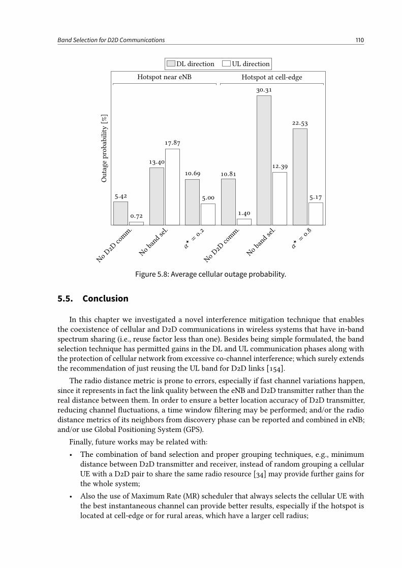
Band Selection for D2D Communications 110
NoD2D
comm.
Nobandsel.
α
⋆=
0.2
NoD2D
comm.
Nobandsel.
α
⋆=
0.8
5.42
13.40
10.69 10.81
30.31
22.53
0.72
17.87
5.00
1.40
12.39
5.17
Hotspot near eNB Hotspot at cell-edge
Outageprobability[%]
DL direction UL direction
Figure 5.8: Average cellular outage probability.
5.5. Conclusion
In this chapter we investigated a novel interference mitigation technique that enablesthe coexistence of cellular and D2D communications in wireless systems that have in-bandspectrum sharing (i.e., reuse factor less than one). Besides being simple formulated, the bandselection technique has permitted gains in the DL and UL communication phases along withthe protection of cellular network from excessive co-channel interference; which surely extendsthe recommendation of just reusing the UL band for D2D links [154].
The radio distance metric is prone to errors, especially if fast channel variations happen,since it represents in fact the link quality between the eNB and D2D transmitter rather than thereal distance between them. In order to ensure a better location accuracy of D2D transmitter,reducing channel uctuations, a time window ltering may be performed; and/or the radiodistance metrics of its neighbors from discovery phase can be reported and combined in eNB;and/or use Global Positioning System (GPS).
Finally, future works may be related with:
• The combination of band selection and proper grouping techniques, e.g., minimumdistance between D2D transmitter and receiver, instead of random grouping a cellularUE with a D2D pair to share the same radio resource [34] may provide further gains forthe whole system;
• Also the use of Maximum Rate (MR) scheduler that always selects the cellular UE withthe best instantaneous channel can provide better results, especially if the hotspot islocated at cell-edge or for rural areas, which have a larger cell radius;
Band Selection for D2D Communications 111
• In a daily use, the trac generated in a network is asymmetric, i.e., the DL band is moreused than the UL band. As such, the operator may limit the D2D-generated interferenceby selecting the less loaded band, especially in a time-based duplexing scheme, wherethe time window for DL can be bigger than the one for UL;
• Evaluate band selection algorithm in real celular networks underlaid by D2D communi-cations;
• An important step in the band selection algorithm is to correctly set the eNB threshold,which controls the amount of UEs that use either band. In this work a procedure has beenproposed which establishes a trade-o between system performance and interferencemitigation. Nevertheless, the best band factor may be based on any other goal, e.g.,reduce the overall system outage probability;
• Also, optimization techniques can be employed to determine the best threshold.
CHAPTER 6
Thesis Conclusion
The thesis was devoted to the general topic of electromagnetic spectrum, especially contem-porary spectrum reuse techniques: TelevisionWhite Spaces (TVWS) and Device-to-Device
(D2D) communications, which foresee in their basis a more exible spectrum management,where primary (licensed or incumbent) and secondary (unlicensed or opportunistic) userscoexist for an improved system capacity.
However, primary users, such as Television (TV) broadcasters or mobile operators, alwaysfeared (unpredictable) interference. Thence, they are mostly reluctant to a exible spectrumuse and do prefer the traditional allocation methods, where the interference from outside worldis controlled or at least predictable. This thesis pretends to be a contribute to diminish that fear,making the spectrum a more democratic place, where all players/actors can aord it, being,therefore, a social catalyzer.
In the rst part the theme of TVWS is explored. We start with a suitable Strengths,Weaknesses, Opportunities, and Threats (SWOT) analysis in chapter 2 in order to identifythe main factors that sustain the reluctancy in their adoption. As a main conclusions, we statethat:
• TVWS defenders shall focus on the promotion of a real-time secondary spectrummarket, where through the correct implementation of policies for protection ratiosin the spectrum broker and geo-location database, incumbents are protected againstinterference;
• Also important is to stimulate the development of innovative business models such thatimportant TV stakeholders, like broadcasters, and mobile operators will make part ofa valuable chain, thus encouraging regulators to develop supportive policies for thefunctioning of secondary spectrum markets.
To encourage the use of TVWS and promote a secondary market for the spectrum, wepresent a tecno-economic evaluation in chapter 3 for three dierent deployment scenarios: onewith 2.60GHz carrier frequency, a second with 700MHz carrier frequency, and a third scenariowith 2.60GHz plus additional TVWS carrier. The rst two are envisioned for a traditionalmarket, while the latter is for the exible secondary spectrummarket. The principal conclusionsare:
• While it is more protable to deploy the network in a lower central carrier frequency(second scenario);
• The secondary market (third scenario) closely approaches the best result;
• On the other hand, the sensitivity analysis revealed that the network protability islittle sensitive to, e.g., the cost of spectrum, price of devices, or device subsidies, beingmoderately sensitive to clients base, and very sensitive to the Average Return Per User(ARPU);
112
Thesis Conclusion 113
• As such, the higher capacity due to the additional TVWS carrier, may allow mobileoperators to increase the ARPU; and/or focus in attracting more clients by employinga strong marketing campaigns and/or promotions (increasing device subsidies and/ordecreasing the price of devices), which would strongly impact in operator’s protability.
The second part of the thesis deals with D2D communications, especially the case whenthey underlay a cellular network. We start with the proposal for a novel neighbor discoverytechnique based on power vectors in chapter 4, which utilizes the already available networkmeasurements, both for the single-cell and multi-cell scenarios. The relevant conclusions maybe summarized in the following manner:
• Results show that with the network help, the time to detect neighbors per Mobile Station(MS) is signicantly reduced, letting more time for the actual data transmission;
• The power of MS consumed during the discovery process is reduced because the mainprocessing is done at the Base Station (BS), building the neighborhood relations, whichfor each MS is considered to be a small set. Thus, just before the session establishment,the MS needs to ensure that D2D communication can be established through the directchannel, e.g., by using a single pair of beacon/acknowledgement packets;
• With the proposed technique no new protocol implementation on signaling is requiredfor the measurement process, because signal quality measurements are already available/exchanged in the network and are mandatory for it to operate. Also, BSs are connectedthough a dedicated link for data control, so no new link is required;
• The multi-cell cases, i.e., MSs that belong to dierent cells (served by dierent BSs) areable to discover each other, enabling the cross-cell border D2D communications.
Chapter 5 is the last technical chapter and it is devoted to the interference mitigation,where by employing the selection of transmission band (either Downlink (DL) or Uplink (UL))for the D2D communication the interference caused in the cellular network is reduced, thuscontributing for an enhanced overall system capacity. The main conclusions may me writtenas follows:
• Despite being a simple concept, in general, band selection improves the gains of cellularcommunications and limits the gains of D2D communications both in DL and UL phases,regardless the position within the cell where the D2D communications happen;
• Also, by using the band selection, the cellular outage probability is always reduced,which reveals the protection provided by the method against harmful interference.
6.1. Future Perspectives
Many works open the door for future improvements, presenting some possible researchdirections. This thesis is no exception. But what is future in the context of wireless systems?As stated in chapter 1, the future is the Fifth Generation (5G) of wireless systems, where thetopics of spectrum sharing [10], Heterogeneous Networks (HetNets) [9], and Machine TypeCommunications (MTCs) [7], [8] are closely related with the contents of the thesis, see gure 6.1(adapted from [4]).
As such, under the umbrella of 5G, future works/research directions, summing up what hasalready been written inside each chapter, may comprise the following:
• Chapter 2. SWOT Analysis for TVWS:
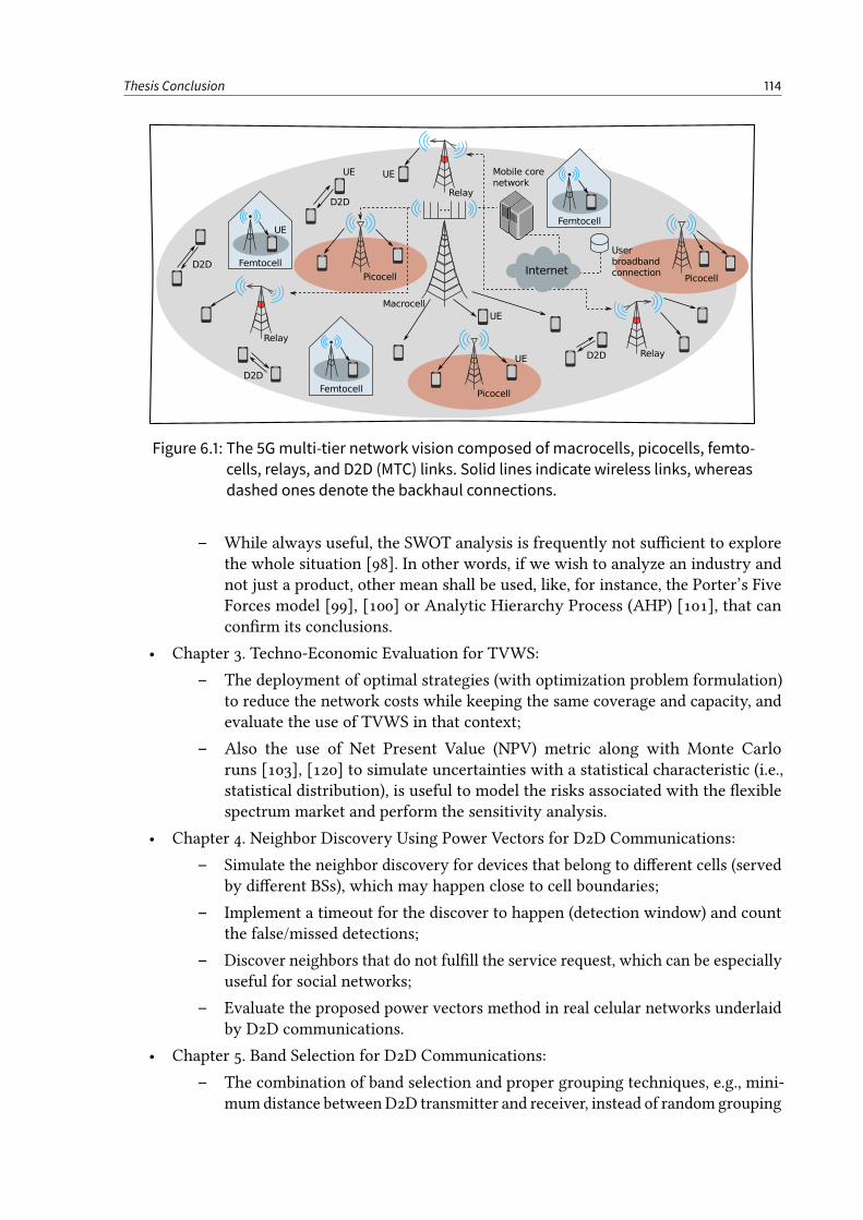
Thesis Conclusion 114
Figure 6.1: The 5Gmulti-tier network vision composed of macrocells, picocells, femto-
cells, relays, and D2D (MTC) links. Solid lines indicate wireless links, whereas
dashed ones denote the backhaul connections.
– While always useful, the SWOT analysis is frequently not sucient to explorethe whole situation [98]. In other words, if we wish to analyze an industry andnot just a product, other mean shall be used, like, for instance, the Porter’s FiveForces model [99], [100] or Analytic Hierarchy Process (AHP) [101], that canconrm its conclusions.
• Chapter 3. Techno-Economic Evaluation for TVWS:
– The deployment of optimal strategies (with optimization problem formulation)to reduce the network costs while keeping the same coverage and capacity, andevaluate the use of TVWS in that context;
– Also the use of Net Present Value (NPV) metric along with Monte Carloruns [103], [120] to simulate uncertainties with a statistical characteristic (i.e.,statistical distribution), is useful to model the risks associated with the exiblespectrum market and perform the sensitivity analysis.
• Chapter 4. Neighbor Discovery Using Power Vectors for D2D Communications:
– Simulate the neighbor discovery for devices that belong to dierent cells (servedby dierent BSs), which may happen close to cell boundaries;
– Implement a timeout for the discover to happen (detection window) and countthe false/missed detections;
– Discover neighbors that do not fulll the service request, which can be especiallyuseful for social networks;
– Evaluate the proposed power vectors method in real celular networks underlaidby D2D communications.
• Chapter 5. Band Selection for D2D Communications:
– The combination of band selection and proper grouping techniques, e.g., mini-mum distance betweenD2D transmitter and receiver, instead of random grouping
Thesis Conclusion 115
a cellular user with a D2D pair to share the same radio resource [34] may providefurther gains for the whole system;
– Also the use of Maximum Rate (MR) scheduler that always selects the cellulardevice with the best instantaneous channel can provide better results, especiallyif the hotspot is located at cell-edge or for rural areas, which have a larger cellradius;
– In a daily use, the trac generated in a network is asymmetric, i.e., the DLband is more used than the UL band. As such, the operator may limit the D2D-generated interference by selecting the less loaded band, especially in a time-based duplexing scheme, where the time window for DL can be bigger than theone for UL;
– Evaluate band selection algorithm in real celular networks underlaid by D2Dcommunications;
– Use other criteria to set the threshold in each cell, which controls the amount ofdevices that use either band. The best band factor may be based on, e.g., reducingthe overall system outage probability;
– Also, optimization techniques can be used to determine the best threshold.

References
[1] Cisco, “Cisco visual networking index: Global mobile data trac forecast update, 2014–2019”, White paper, Feb. 2015, pp. 1–42. [Online]. Available: http://www.cisco.com/c/en/us/solutions/collateral/service- provider/visual-
networking-index-vni/white_paper_c11-520862.pdf (visited on 10/2015).
[2] Ericsson, RWS-120003 LTE release 12 and beyond, 3GPP Radio Access NetworkWorkshopon Release 12 and Onwards, Ljubljana, Slovenia, Jun. 2012.
[3] J. G. Andrews, S. Buzzi, W. Choi, S. V. Hanly, A. Lozano, A. C. K. Soong, and J. C. Zhang,“What will 5G be?”, IEEE Journal on Selected Areas in Communications, vol. 32, no. 6,pp. 1065–1082, Jun. 2014, issn: 0733-8716. doi: 10.1109/JSAC.2014.2328098.
[4] E. Hossain, M. Rasti, H. Tabassum, and A. Abdelnasser, “Evolution toward 5G multi-tiercellular wireless networks: An interference management perspective”, IEEE Wireless
Communications, vol. 21, no. 3, pp. 118–127, Jun. 2014, issn: 1536-1284. doi: 10.1109/MWC.2014.6845056.
[5] E. G. Larsson, F. Tufvesson, O. Edfors, and T. L. Marzetta, “Massive MIMO for nextgeneration wireless systems”, IEEE Communications Magazine, vol. 52, no. 2, pp. 186–195,Feb. 2014, issn: 0163-6804. doi: 10.1109/MCOM.2014.6736761.
[6] S. Rangan, T. S. Rappaport, and E. Erkip, “Millimeter wave cellular wireless networks:Potentials and challenges”, Proceedings of the IEEE, vol. 102, no. 3, pp. 366–385, Feb. 2014,issn: 0018-9219. doi: 10.1109/JPROC.2014.2299397.
[7] S. Mumtaz, K. M. S. Huq, and J. Rodriguez, “Direct mobile-to-mobile communication:Paradigm for 5G”, IEEE Wireless Communications, vol. 21, no. 5, pp. 14–23, Oct. 2014,issn: 1536-1284. doi: 10.1109/MWC.2014.6940429.
[8] L. Wei, R. Q. Hu, Y. Qian, and G. Wu, “Enable device-to-device communications un-derlaying cellular networks: Challenges and research aspects”, IEEE Communications
Magazine, vol. 52, no. 6, pp. 90–96, Jun. 2014, issn: 0163-6804. doi: 10.1109/MCOM.2014.6829950.
[9] J. G. Andrews, “Seven ways that hetnets are a cellular paradigm shift”, IEEE Com-
munications Magazine, vol. 51, no. 3, pp. 136–144, Mar. 2013, issn: 0163-6804. doi:10.1109/MCOM.2013.6476878.
[10] J. Mitola III et al., “Accelerating 5G QoE via public-private spectrum sharing”, IEEECommunications Magazine, vol. 52, no. 5, pp. 77–85, May 2014, issn: 0163-6804. doi:10.1109/MCOM.2014.6815896.
[11] T. M. Taher, R. B. Bacchus, K. J. Zdunek, and D. A. Roberson, “Long-term spectraloccupancy ndings in chicago”, in 2011 IEEE Symposium on Dynamic Spectrum Access
Networks (DySpan), May 2011, pp. 100–107. doi: 10.1109/DYSPAN.2011.5936195.
116
References 117
[12] A. Palaios, J. Riihijärvi, O. Holland, and P. Mähönen, “A week in London: Spectrum usagein metropolitan London”, in IEEE 24th Annual International Symposium on Personal,
Indoor, and Mobile Radio Communications (PIMRC), Sep. 2013, pp. 2532–2537. doi: 10.1109/PIMRC.2013.6666571.
[13] M. Prazy, “The protability analysis of the multi-band spectrum broker”, in IEEE 24th
Annual International Symposium on Personal, Indoor, and Mobile Radio Communications
(PIMRC), Sep. 2013, pp. 3454–3458. doi: 10.1109/PIMRC.2013.6666742.
[14] OFCOM, “Digital dividend review: Geographic interleaved awards 470–550MHz and630–790MHz”, Consultation, Jun. 2008.
[15] E. C. C. (ECC), “Technical considerations regarding harmonisation options for the digitaldividend”, Compatibility issues between “cellular / low power transmitter” networks and“larger coverage / high power / tower” type of networks, European Conference of Postaland Telecommunications Administrations (CEPT), CEPT Report 21, Mar. 2007. [Online].Available: www.erodocdb.dk/docs/doc98/official/pdf/CEPTREP021.pdf(visited on 10/2015).
[16] , “Technical considerations regarding harmonisation options for the digital div-idend”, A preliminary assessment of the feasibility of tting new/future applica-tions/services into non-harmonised spectrum of the digital dividend (namely theso-called “white spaces” between allotments), European Conference of Postal andTelecommunications Administrations (CEPT), CEPT Report 24, Jun. 2008. [Online].Available: http : / / www . erodocdb . dk / docs / doc98 / official / pdf /CEPTRep024.pdf (visited on 10/2015).
[17] COGEU, “European TV white spaces analysis and COGEU use-cases”, Deliverable2.1, Mar. 2010, Version 1.0. [Online]. Available: http://www.ict-cogeu.eu/deliverables.html (visited on 10/2015).
[18] OFCOM, “Implementing TV white spaces”, Statement, Feb. 2015. [Online]. Available:http://stakeholders.ofcom.org.uk/binaries/consultations/white-
space-coexistence/statement/tvws-statement.pdf (visited on 10/2015).
[19] FCC, “In the matter of unlicensed operation in the TV broadcast bands: Et docket no.04-186”, Washington D.C., Order DA 11-131, Jan. 2011.
[20] A. Yang, Overview of FCC’s new rules for TV white space devices and database updates,ITU-R SG 1/WP 1B Workshop: Spectrum Management Issues on the Use of WhiteSpaces By Cognitive Radio Systems, Geneva, Switzerland, Jan. 2014. [Online]. Available:http://www.itu.int/en/ITU-R/study-groups/workshops/RWP1B-
SMWSCRS-14/Presentations/USA%20-%20Overview%20of%20FCC%E2%80%
99s%20New%20Rules%20for%20TV%20White%20Space%20Devices%20and%
20database%20updates.pdf (visited on 10/2015).
[21] FCC, Et docket no. 04-186, Washington D.C., Sep. 2014. [Online]. Available: https://apps.fcc.gov/edocs_public/attachmatch/DA-14-1309A1.pdf (visitedon 10/2015).
[22] C. A. A. Afonso, “New cognitive radio technologies, white spaces and the digital dividendin the brazilian context”, in TV White Spaces: A Pragmatic Approach, E. Pietrosemoliand M. Zennaro, Eds., 1st ed., The Abdus Salam International Centre for TheoreticalPhysics, Dec. 2013, pp. 43–50, isbn: 978-9295003-50-7.
References 118
[23] E. Obregon, K. W. Sung, and J. Zander, “On the sharing opportunities for ultra-densenetworks in the radar bands”, in 2014 IEEE International Symposium onDynamic Spectrum
Access Networks (DySpan), Apr. 2014, pp. 215–223. doi: 10.1109/DySPAN.2014.6817798.
[24] H. Bogucka, M. Parzy, P. Marques, J. W. Mwangoka, and T. Forde, “Secondary spectrumtrading in TV white spaces”, IEEE Communications Magazine, vol. 50, no. 11, pp. 121–129,Nov. 2012. doi: 10.1109/MCOM.2012.6353691.
[25] “Terrestrial trunked radio (TETRA); voice plus data (V+D); part 2: Air interface (AI)”,European Telecommunications Standards Institute (ETSI), ETSI TS 100 392-2, Oct. 2011,Version 3.5.1. [Online]. Available: http://www.etsi.org/deliver/etsi_ts/100300_100399/10039202/03.05.01_60/ts_10039202v030501p.pdf (visitedon 08/2012).
[26] G. Fodor, E. Dahlman, G. Mildh, S. Parkvall, N. Reider, G. Miklós, and Z. Turányi, “Designaspects of network assisted device-to-device communications”, IEEE Communications
Magazine, vol. 50, no. 3, pp. 170–176, Mar. 2012, issn: 0163-6804. doi: 10.1109/MCOM.2012.6163598.
[27] K. Doppler, M. Rinne, C. Wijting, C. B. Ribeiro, and K. Hugl, “Device-to-device commu-nication as an underlay to LTE-advanced”, IEEE Communications Magazine, vol. 47, no.12, pp. 42–49, Dec. 2009, issn: 0163-6804. doi: 10.1109/MCOM.2009.5350367.
[28] M. S. Corson, R. Laroia, J. Li, V. Park, T. Richardson, and G. Tsirtsis, “Toward proximity-aware internetworking”, IEEE Wireless Communications, vol. 17, no. 6, pp. 26–33, Dec.2010, issn: 1536-1284. doi: 10.1109/MWC.2010.5675775.
[29] L. Lei, Z. Zhong, C. Lin, and X. Shen, “Operator controlled device-to-device commu-nications in LTE-advanced networks”, IEEE Wireless Communications, vol. 19, no. 3,pp. 96–104, Jun. 2012, issn: 1536-1284. doi: 10.1109/MWC.2012.6231164.
[30] J. M. B. da Silva Jr., G. Fodor, and T. F. Maciel, “Performance analysis of network-assistedtwo-hop D2D communications”, in IEEE Global Communications Conference Workshops
(GC’14 Wkshps), Dec. 2014, pp. 1050–1056. doi: 10.1109/GLOCOMW.2014.7063572.
[31] 3GPP, “Feasibility study for proximity services (ProSe)”, 3rd Generation PartnershipProject (3GPP), TR 22.803, Jun. 2013. [Online]. Available: http://www.3gpp.org/ftp/specs/html-info/22803.htm (visited on 06/2014).
[32] P. Phunchongharn, E. Hossain, and D. I. Kim, “Resource allocation for device-to-devicecommunications underlaying LTE-advanced network”, IEEE Communications Magazine,vol. 20, no. 4, pp. 91–100, Aug. 2013, issn: 1536-1284. doi: 10.1109/MWC.2013.6590055.
[33] G. Fodor, D. D. Penda, M. Belleschi, and M. Johansson, “A comparative study of powercontrol approaches for device-to-device communications”, in IEEE International Confer-
ence on Communications (ICC’13), Budapest, Hungary: IEEE, Jun. 2013.
[34] J. M. B. da Silva Jr., T. F. Maciel, R. L. Batista, C. F. M. e Silva, and F. R. P. Cavalcanti,“UE grouping and mode selection for D2D communications underlaying a multicellularwireless system”, in IEEE WCNC 2014 - Workshop on Device-to-Device and Public Safety
Communications (WCNC’14 -WDPCWorkshop), Istambul, Turkey, Apr. 2014, pp. 230–235.
References 119
[35] K. Doppler, C.-H. Yu, C. B. Ribeiro, and P. Jänis, “Mode selection for device-to-devicecommunication underlaying an LTE-advanced network”, in IEEE Wireless Communica-
tions and Networking Conference (WCNC’10), Apr. 2010, pp. 1–6. doi: 10.1109/WCNC.2010.5506248.
[36] P. Jänis, V. Koivunen, C. B. Ribeiro, K. Doppler, and K. Hugl, “Interference-avoidingMIMO schemes for device-to-device radio underlaying cellular networks”, in IEEE 20th
Personal, Indoor and Mobile Radio Communications Symposium (PIMRC’09), Sep. 2009,pp. 2385–2389, isbn: 978-1-4244-5122-7. doi: 10.1109/PIMRC.2009.5450284.
[37] C.-H. Yu, O. Tirkkonen, K. Doppler, and C. B. Ribeiro, “Power optimization of device-to-device communication underlaying cellular communication”, in IEEE International
Conference on Communications (ICC’09), Jun. 2009, pp. 1–5. doi: 10.1109/ICC.2009.5199353.
[38] Y. V. L. de Melo, R. L. Batista, C. F. M. e Silva, T. F. Maciel, J. M. B. da Silva Jr., and F. R. P.Cavalcanti, “Power control schemes for energy eciency of cellular and device-and-device communications”, in IEEE Wireless Communications and Networking Conference
(WCNC’15), Mar. 2015, pp. 1690–1694. doi: 10.1109/WCNC.2015.7127722.
[39] , “Uplink power control with variable target SINR for D2D communications under-lying cellular networks”, in IEEE 81st Vehicular Technology Conference (VTC 2015-Spring),May 2015, pp. 1–5. doi: 10.1109/VTCSpring.2015.7146150.
[40] R. Tanbourgi, H. Jäkel, and F. K. Jondral, “Cooperative interference cancellation usingdevice-to-device communications”, IEEE Communications Magazine, vol. 52, no. 6,pp. 118–124, Jun. 2014, issn: 0163-6804. doi: 10.1109/MCOM.2014.6829953.
[41] S. Xu and K. S. Kwak, “Eective interference coordination for D2D underlaying LTEnetworks”, in IEEE 79th Vehicular Technology Conference (VTC 2014-Spring), May 2014,pp. 1–5. doi: 10.1109/VTCSpring.2014.7022897.
[42] G. Fodor, A. Pradini, and A. Gattami, “On applying network coding in network assisteddevice-to-device communications”, in Proceedings of 20th European Wireless (EW’14),Barcelona, Spain, May 2014.
[43] C. F. M. Silva, J. M. B. Silva Jr., and T. F. Maciel, “Radio resource management fordevice-to-device communications in long term evolution networks”, in Resource Allo-
cation and MIMO for 4G and Beyond, F. R. P. Cavalcanti, Ed., New York, USA: SpringerScience+Business Media, 2014, pp. 105–156, isbn: 978-1-4614-8056-3. doi: 10.1007/978-1-4614-8057-0_3.
[44] A. Asadi, Q. Wang, and V. Mancuso, “A survey on device-to-device communication incellular networks”, IEEE Communications Surveys and Tutorials, vol. 16, no. 4, pp. 1801–1819, Apr. 2014, issn: 1553-877X. doi: 10.1109/COMST.2014.2319555.
[45] C. F. Silva, H. Alves, and Á. Gomes, “Extension of LTE operational mode over TV whitespaces”, in Future Network and Mobile Summit 2011 Conference Proceedings, Warsaw,Poland, Jun. 2011, pp. 1–13. [Online]. Available: http://www.ict-cogeu.eu/pdf/publications/Y2/FUNEMS_2011_COGEU_paper_n2.pdf (visited on 10/2015).
[46] C. Dosch, J. Kubasik, and C. F. M. Silva, “TVWS policies to enable ecient spectrumsharing”, in 22nd European Regional Conference of the International Telecommunications
Society (ITS 2011), Budapest, Hungary, Sep. 2011, pp. 1–26. [Online]. Available: http://hdl.handle.net/10419/52145 (visited on 10/2015).
References 120
[47] C. F. M. Silva, F. R. P. Cavalcanti, and Á. Gomes, “SWOT analysis for TV white spaces”,Transactions on Emerging Telecommunications Technologies, vol. 26, no. 6, pp. 957–974,Jun. 2015, Published online: Dec. 2013, issn: 2161-3915. doi: 10.1002/ett.2770.
[48] C. F. M. e Silva and R. L. Batista, “Methods, nodes and user equipments for nding neigh-boring user equipments with which a rst user equipment may be able to communicatedirectly”, P43774WO, Jul. 2014.
[49] C. F. M. e Silva, T. F. Maciel, R. L. Batista, L. Elias, A. Robson, and F. R. P. Cavalcanti,“Network-assisted neighbor discovery based on power vectors for D2D communications”,in IEEE 81st Vehicular Technology Conference (VTC 2015-Spring), May 2015, pp. 1–5, isbn:978-1-4799-8088-8.
[50] C. F. M. e Silva, R. L. Batista, J. M. B. Silva Jr., T. F. Maciel, and F. R. P. Cavalcanti, “Inter-ference mitigation using band selection for network-assisted D2D communications”, inIEEE 81st Vehicular Technology Conference (VTC 2015-Spring), May 2015, pp. 1–5, isbn:978-1-4799-8088-8.
[51] C. F. M. e Silva and G. Fodor, “Method and system of a wireless communication networkfor detecting neighbouring UEs, of a rst UE”, P47887WO, Nov. 2015.
[52] R. L. Batista, C. F. M. e Silva, J. M. B. da Silva Jr., T. F. Maciel, and F. R. P. Cavalcanti,“Impact of device-to-device communications on cellular communications in a multi-cellscenario”, inXXXI Telecommunications Brazilian Symposium (SBrT2013), Fortaleza, Brazil,Sep. 2013. doi: 10.14209/sbrt.2013.241.
[53] R. L. Batista, C. F. M. e Silva, J. M. B. da Silva Jr., T. F. Maciel, and F. R. P. Cavalcanti,“What happens with a proportional fair cellular scheduling when D2D communicationsunderlay a cellular network?”, in IEEE WCNC 2014 - Workshop on Device-to-Device and
Public Safety Communications (WCNC’14 - WDPC Workshop), Istambul, Turkey, Apr.2014, pp. 260–265.
[54] R. L. Batista, C. F. M. e Silva, T. F. Maciel, and F. R. P. Cavalcanti, “Method and radionetwork node for scheduling of wireless devices in a cellular network”, P42550WO, Apr.2014.
[55] R. L. Batista, C. F. M. e Silva, J. M. B. da Silva Jr., T. F. Maciel, and F. R. P. Cavalcanti,“Power prediction prior to scheduling combined with equal power allocation for theOFDMA UL”, in Proceedings of 20th European Wireless (EW’14), Barcelona, Spain, May2014.
[56] R. L. Batista, C. F. M. e Silva, T. F. Maciel, J. M. B. da Silva Jr., and F. R. P. Cavalcanti,“Joint opportunistic scheduling of cellular and D2D communications”, IEEE Transactions
on Vehicular Technology, Submitted, issn: 0018-9545.
[57] J. M. B. da Silva Jr., T. F. Maciel, C. F. M. e Silva, R. L. Batista, and Y. V. L. de Melo,“Spatial user grouping for D2D communications underlying a multi-cell wireless system”,EURASIP Journal on Wireless Communications and Networking, Submitted, issn: 1687-1499.
[58] Y. V. L. de Melo, R. L. Batista, T. F. Maciel, C. F. M. e Silva, J. M. B. da Silva Jr., and F. R. P.Cavalcanti, “Power control with variable target SINR for D2D communications under-lying cellular networks”, in Proceedings of 20th European Wireless (EW’14), Barcelona,Spain, May 2014.
References 121
[59] A. R. F. de Oliveira, L. Elias, C. F. M. e Silva, T. F. Maciel e F. R. P. Cavalcanti, «Descobertade vizinhos baseada em vetores de potência para comunicações D2D [Neighbor discoverybased on power vectors for D2D communications]», em XXXIII Telecommunications
Brazilian Symposium (SBrT2015), Original document in Portuguese, set. de 2015, pp. 1–2.
[60] ETSI, “Recongurable radio systems (RRS); use cases for operation in white spacefrequency bands”, TR 102 907, Oct. 2011, Version 1.1.1.
[61] J. Mitola III and G. Q. Maguire Jr., “Cognitive radio: Making software radios morepersonal”, IEEE Personal Communications, vol. 6, no. 4, pp. 13–18, Aug. 1999. doi: 10.1109/98.788210.
[62] J. Mitola III, “Cognitive radio: An integrated agent architecture for software denedradio”, PhD thesis, Royal Institute of Technology (KTH), Stockholm, Sweden, May 2000.
[63] S. Mangold, L. Berlemann, and S. Nandagopalan, “Spectrum sharing with value-orienta-tion for cognitive radio”, European Transactions on Telecommunications, vol. 17, no. 3,pp. 383–394, May 2006. doi: 10.1002/ett.1120.
[64] COGEU, “Initial architecture for TVWS spectrum sharing systems”, Deliverable 3.2, Jan.2011, Version 3.0. [Online]. Available: http://www.ict-cogeu.eu/deliverables.html (visited on 10/2015).
[65] L. Bicho e S. Baptista, Modelo de porter e análise SWOT: Estratégias de negócio [por-
ter’s model and SWOT analysis: Business strategies], Instituto Politécnico de Coimbra:Departamento de Engenharia Civil, Original document in Portuguese, dez. de 2006.
[66] A. Chapman, SWOT analysis: SWOT analysis method and examples, with free SWOT
template, 2005–2011. [Online]. Available: http://www.businessballs.com/swotanalysisfreetemplate.htm (visited on 07/2011).
[67] J. M. Chapin and W. H. Lehr, “The path to market success for dynamic spectrum accesstechnology”, IEEE Communications Magazine, vol. 45, no. 5, pp. 96–103, May 2007. doi:10.1109/MCOM.2007.358855.
[68] E. C. Committee, “Technical and operational requirements for the possible operationof cognitive radio systems in the ‘white spaces’ of the frequency band 470–790MHz”,Cardi, ECC Report 159, Jan. 2011. [Online]. Available: http://www.erodocdb.dk/docs/doc98/official/Pdf/ECCRep159.pdf (visited on 12/2011).
[69] M. Nekovee, “A survey of cognitive radio access to TV white spaces”, InternationalJournal of Digital Multimedia Broadcasting, vol. 2010, pp. 1–12, 2010.
[70] FCC, “In the matter of unlicensed operation in the TV broadcast bands: Et docket no.04-186”, Washington D.C., Second Memorandum Opinion and Order FCC 10-174, Sep.2010.
[71] COGEU, “Policies to enable ecient spectrum sharing over TVWS at European level”,Deliverable 2.2, Mar. 2011, Version 1.0. [Online]. Available: http://www.ict-cogeu.eu/deliverables.html (visited on 10/2015).
[72] M. Parzy and H. Bogucka, “Non-identical objects auction for spectrum sharing in TVwhite spaces—the perspective of service providers as secondary users”, in 2011 IEEE
Symposium on Dynamic Spectrum Access Networks (DySpan), May 2011, pp. 389–398.doi: 10.1109/DYSPAN.2011.5936228.
References 122
[73] ANACOM, «Projecto de decisão sobre a limitação do número de direitos de utilização defrequências nas faixas dos 450MHz, 800MHz, 900MHz, 1800MHz, 2.10GHz e 2.60GHze denição do respectivo procedimento de atribuição [Decision project about the limita-tion in the number of utilization rights for the frequencies in bands of 450MHz, 800MHz,900MHz, 1800MHz, 2.10GHz and 2.60GHz and denition of respective attributionprocedure]», Deliberação 17.03.2011, mar. de 2011, Original document in Portuguese.
[74] , «Projecto de regulamento do leilão para a atribuição de direitos de utilização defrequências nas faixas dos 450MHz, 800MHz, 900MHz, 1800MHz, 2.10GHz e 2.60GHz[Regulation project for the attribution of usage rights of frequencies in the bandsof 450MHz, 800MHz, 900MHz, 1800MHz, 2.10GHz and 2.60GHz]», Regulamento,mar. de 2011, Original document in Portuguese.
[75] M. Cave, Anti-competitive behaviour in spectrum markets, Apr. 2009.
[76] ERG-RSPG, “ERG-RSPG report on radio spectrum competition issues”, ERG (09) 22, Jun.2009.
[77] R. Murty, R. Chandra, T. Moscibroda, and P. Bahl, “Senseless: A database-driven whitespaces network”, in 2011 IEEE Symposium on Dynamic Spectrum Access Networks (DyS-
pan), May 2011, pp. 10–21. doi: 10.1109/DYSPAN.2011.5936197.
[78] D. Makris, G. Gardikis, and A. Kourtis, “Quantifying TV white space capacity: Ageolocation-based approach”, IEEE Communications Magazine, vol. 50, no. 9, pp. 145–152,Sep. 2012. doi: 10.1109/MCOM.2012.6295725.
[79] E. C. C. (ECC), “Technical considerations regarding harmonisation options for the digitaldividend in the European Union”, Guideline on cross border coordination issues betweenmobile services in one country and broadcasting services in another country, EuropeanConference of Postal and Telecommunications Administrations (CEPT), CEPT Report29, Jun. 2009. [Online]. Available: www.erodocdb.dk/docs/doc98/official/pdf/CEPTREP029.pdf (visited on 10/2015).
[80] GSMA, Digital dividend for mobile: Bringing broadband to all, Brochure, 2009. [Online].Available: http://www.gsma.com/spectrum/wp-content/uploads/2012/07/Spectrum-Digital-dividend-for-mobile-English.pdf (visited on 10/2015).
[81] COGEU, “Final architecture for TVWS spectrum sharing systems”, Deliverable 3.3, Sep.2011, Version 1.0. [Online]. Available: http://www.ict-cogeu.eu/deliverables.html (visited on 10/2015).
[82] E. Parliament and Council, Multi-annual radio spectrum policy programme, Feb. 2012.
[83] OFCOM, “Simplifying spectrum trading—spectrum leasing and other market enhance-ments”, Final statement, Jun. 2011.
[84] M. Baker, LTE-advanced physical layer, IMT-Advanced Evaluation Workshop, Beijing,Dec. 2009.
[85] A. Solheim, Choosing the backhaul for LTE, Mar. 2009. [Online]. Available: http://www.mobilitytechzone.com/topics/4g-wirelessevolution/articles/
52237-choosing-backhaul-lte.htm (visited on 08/2011).
[86] Cisco, “Cisco visual networking index: Global mobile data trac forecast update, 2011–2016”, White paper, Feb. 2012, pp. 1–29. [Online]. Available: http://www.efocus.sk/images/uploads/cisco_data_trafic_2016.pdf (visited on 10/2015).
References 123
[87] M. Nekovee, “Current trends in regulation of secondary access to TV white spaces usingcognitive radio”, in IEEE GLOBECOM 2011, Accepted, Houston, Dec. 2011.
[88] S. Y. Tan, R. Karimi, A. Gowans, and D. Donachie, “Draft regulatory requirements forwhite space devices in the UHF TV band”, OFCOM, Discussion document, Feb. 2012,Draft.
[89] G. Yuan, X. Zhang, W.Wang, and Y. Yang, “Carrier aggregation for LTE-advanced mobilecommunication systems”, IEEE Communications Magazine, vol. 48, no. 2, pp. 88–93, Feb.2010.
[90] M. Baker, “From LTE-advanced to the future”, IEEE Communications Magazine, vol. 50,no. 2, pp. 116–120, Feb. 2012. doi: 10.1109/MCOM.2012.6146490.
[91] ITU, Resolution ITU-R 58, Studies on the implementation and use of cognitive radio systems,Jan. 2012.
[92] OFCOM, Ofcom progresses plans for new wireless technology, Nov. 2010. [Online]. Avail-able: http://media.ofcom.org.uk/2010/11/09/ofcom-progresses-plans-for-new-wireless-technology/ (visited on 08/2011).
[93] E. Commission, “Promoting the shared use of radio spectrum resources in the inter-nal market”, Communication from the Commission to the European Parliament, theCouncil, the European Economic and Social Committee and the Committee of RegionsCOM(2012) 478 nal, Sep. 2012. [Online]. Available: http://eur-lex.europa.eu/LexUriServ/LexUriServ.do?uri=COM:2012:0478:FIN:EN:PDF.
[94] OFCOM, “Implementing geolocation”, Consultation, Dec. 2011.
[95] ITU and W. Bank, Dispute resolution in the telecommunications sector: Current practices
and future directions, Oct. 2004.
[96] H. Assef, The meaning of reconciliation, European Centre for Conict Prevention, May1999. [Online]. Available: http://www.gppac.net/documents/pbp/part1/2_
reconc.htm (visited on 08/2011).
[97] P. Xavier, Licensing of third generation (3G) mobile: Brieng paper, ITU-InternationalTelecommunication Union: 3G Licensing Workshop, Sep. 2001.
[98] N. Pahl and A. Richter, SWOT Analysis—Idea, Methodology And A Practical Approach.GRIN Academic Publishing, 2007, isbn: 978-3-640-30303-8.
[99] H. de Swaan Arons and P. Waalewijn, A knowledge base representing Porter’s ve forces
model, Rotterdam: Erasmus University, 1999.
[100] M. H. Evans, Course 12: Competitive intelligence (part 2 of 2), Excellence in FinancialManagement, 2004.
[101] T. L. Saaty, Decision Making for Leaders: The Analytic Hierarchy Process for Decisions in a
Complex World, 3rd ed. Pittsburgh, USA: RWS Publications, 2012, isbn: 0-9620317-8-X.
[102] S. Bichler and J. Nitzan, Systemic fear, modern nance and the future of capitalism,Jerusalem and Montreal, Jul. 2010. [Online]. Available: http://bnarchives.yorku.ca/289/03/20100700_bn_systemic_fear_modern_finance_future_of_
capitalism.pdf (visited on 10/2015).
[103] S. C. Savvides, “Risk analysis in investment appraisal”, Project Appraisal, vol. 9, no. 1,pp. 3–18, Mar. 1994. [Online]. Available: https://mpra.ub.uni-muenchen.de/10035/1/MPRA_paper_10035.pdf (visited on 10/2015).
References 124
[104] V. Maroyi, “Capital budgeting practices: A South African perspective”, Master’s thesis,Wageningen University, Wageningen, Netherlands, Aug. 2011.
[105] COGEU, “Spectrum-aware routing, transport protocols and negotiation protocols be-tween players for secondary spectrum trading; system level simulation tool - initialspecication”, Deliverable 6.2, Dec. 2011, Version 1.0. [Online]. Available: http://www.ict-cogeu.eu/deliverables.html (visited on 10/2015).
[106] F. J. Gallego, Mapping rural/urban areas from population density grids, Ispra, Italy:Institute for Environment and Sustainability, JRC, 2004. [Online]. Available: http://www.ec- gis.org/docs/F11116/RURAL%5C%20URBAN%5C%20%5C%
20POPDENS.PDF (visited on 10/2015).
[107] L. Dijkstra and H. Poelman, European Commission, Working Papers 01/2014, May2014. [Online]. Available: http://ec.europa.eu/regional_policy/en/information / publications / working - papers / 2014 / a - harmonised -
definition - of - cities - and - rural - areas - the - new - degree - of -
urbanisation (visited on 10/2015).
[108] E. Dahlman, S. Parkvall, and J. Sköld, 4G: LTE/LTE-Advanced for Mobile Broadband, 1st ed.Elsevier, Academic Press, 2011, isbn: 978-0-12-385489-6.
[109] V. Erceg, L. J. Greenstein, S. Y. Tjandra, S. R. Parko, A. Gupta, B. Kulic, A. A. Julius, andR. Bianchi, “An empirically based path loss model for wireless channels in suburbanenvironments”, IEEE Journal on Selected Areas in Communications, vol. 17, no. 7, pp. 1205–1211, Jul. 1999, issn: 0733-8716. doi: 10.1109/49.778178.
[110] V. Erceg et al., IEEE 802.16 Broadband Wireless Access Working Group, IEEE 802.16.3c-01/29r4, Jul. 2001. [Online]. Available: http://www.ieee802.org/16/tg3/contrib/802163c-01_29r4.pdf (visited on 10/2015).
[111] M. Hata, “Empirical formula for propagation loss in land mobile radio services”, IEEETransactions on Vehicular Technology, vol. 29, no. 3, pp. 317–325, Aug. 1980, issn: 0018-9545. doi: 10.1109/T-VT.1980.23859.
[112] A. B. Syed, “Dimensioning of LTE network. Description of models and tools, cover-age and capacity estimation of 3GPP long term evolution”, Master’s thesis, HelsinkiUniversity of Technology, Helsinki, Finland, Feb. 2009.
[113] P. Vieira, P. Queluz, and A. Rodrigues, “LTE spectral eciency using spatial multiplex-ing MIMO for macro-cells”, in 2nd International Conference on Signal Processing and
Communication Systems (ICSPCS’08), Dec. 2008, pp. 1–6, isbn: 978-1-4244-4243-0. doi:10.1109/ICSPCS.2008.4813660.
[114] 3GPP, “Evolved universal terrestrial radio access (E-UTRA); base station (BS) radiotransmission and reception”, 3rd Generation Partnership Project (3GPP), TS 36.104,Sep. 2012. [Online]. Available: http://www.3gpp.org/ftp/Specs/html-info/36104.htm (visited on 04/2014).
[115] , “Evolved universal terrestrial radio access (E-UTRA); physical layer procedures”,3rd Generation Partnership Project (3GPP), TS 36.213, Mar. 2008. [Online]. Available:http://www.3gpp.org/ftp/specs/html-info/36213.htm (visited on 04/2014).
[116] Motorola, Motorola WBC 700 portfolio, Jan. 2010.
[117] D. Dababneh, “LTE trac generation and evolved packet core (EPC) network planning”,Master’s thesis, Carleton University, Ottawa, Canada, Mar. 2013.
References 125
[118] FUTON, “Architecture, business evaluation and deployment models: Final vision atthe end of FUTON”, Deliverable 2.3, Sep. 2010, Version 1.2. [Online]. Available: http://www.ict-futon.eu/private/docs/deliverables/d2.3.pdf (visited on10/2015).
[119] C. F. Silva and V. S. Ribeiro, “Business evaluation for FUTON-like architectures”, in IEEE
International Conference on Computer as a Tool (EUROCON’11), Apr. 2011, pp. 1–4, isbn:978-1-4244-7486-8. doi: 10.1109/EUROCON.2011.5929345.
[120] M. v. Bredow and G. Reinhart, “Method to evaluate the protability and risk structureof projects in the automotive industry”, in IEEE International Conference on Industrial
Engineering and Engineering Management (IEEM’09), Dec. 2009, pp. 1588–1592, isbn:978-1-4244-4869-2. doi: 10.1109/IEEM.2009.5373105.
[121] M. Belleschi, G. Fodor, and A. Abrardo, “Performance analysis of a distributed resourceallocation scheme for D2D communications”, in IEEE Global Communications Conference
Workshops (GC’11 Wkshps), Dec. 2011, pp. 358–362, isbn: 978-1-4673-0039-1. doi: 10.1109/GLOCOMW.2011.6162471.
[122] S. Vasudevan, J. Kurose, and D. Towsley, “On neighbor discovery in wireless networkswith directional antennas”, in 24th Annual Joint Conference of the IEEE Computer and
Communications Societies (INFOCOM’05), vol. 4, Mar. 2005, pp. 2502–2512. doi: 10.1109/INFCOM.2005.1498535.
[123] D. Angelosante, E. Biglieri, and M. Lops, “Neighbor discovery in wireless networks: Amultiuser-detection approach”, Physical Communication, vol. 3, no. 1, pp. 28–36, 2010,issn: 1874-4907. doi: 10.1016/j.phycom.2009.08.005.
[124] K. Doppler, C. B. Ribeiro, and J. Kneckt, “Advances in D2D communications: Energyecient service and device discovery radio”, in 2nd International Conference on Wireless
Communication, Vehicular Technology, Information Theory and Aerospace & Electronic
Systems Technology (Wireless VITAE’11), Mar. 2011, pp. 1–6, isbn: 978-1-4577-0787-2.doi: 10.1109/WIRELESSVITAE.2011.5940857.
[125] S. Vasudevan, D. Towsley, D. Goeckel, and R. Khalili, “Neighbor discovery in wirelessnetworks and the coupon collector’s problem”, in Proceedings of the 15th Annual In-
ternational Conference on Mobile Computing and Networking (MobiCom’09), Sep. 2009,pp. 181–192, isbn: 978-1-60558-702-8. doi: 10.1145/1614320.1614341.
[126] L. Zhang and D. Guo, “Neighbor discovery in wireless networks using compressedsensing with Reed-Muller codes”, in International Symposium on Modeling and Opti-
mization in Mobile, Ad Hoc, and Wireless Networks (WiOpt’11), May 2011, pp. 154–160,isbn: 978-1-61284-824-2. doi: 10.1109/WIOPT.2011.5930008.
[127] L. You, Z. Yuan, P. Yang, andG. Chen, “ALOHA-like neighbor discovery in low-duty-cyclewireless sensor networks”, in IEEE Wireless Communications and Networking Conference
(WCNC’11), vol. 4, Mar. 2011, pp. 749–754. doi: 10.1109/WCNC.2011.5779256.
[128] G. Camarillo, “Peer-to-peer (P2P) architecture: Denition, taxonomies, examples, andapplicability”, RFC Editor, RFC 5694, Nov. 2009, pp. 1–26. [Online]. Available: http://www.rfc-editor.org/rfc/rfc5694.txt.
[129] D. Angelosante, E. Biglieri, and M. Lops, “A simple algorithm for neighbor discoveryin wireless networks”, in IEEE International Conference on Acoustics, Speech and Signal
Processing (ICASSP’07), vol. 3, Apr. 2007, pp. III-169–III-172. doi: 10.1109/ICASSP.2007.366499.
References 126
[130] Z. Zhang and B. Li, “Neighbor discovery in mobile ad hoc self-conguring networkswith directional antennas: Algorithms and comparisons”, IEEE Transactions on Wireless
Communications, vol. 7, no. 5, pp. 1540–1549, May 2008, issn: 1536-1276. doi: 10.1109/TWC.2008.05908.
[131] E. Felemban, R. Murawski, E. Ekici, S. Park, K. Lee, J. Park, and Z. Hameed, “Sand:Sectored-antenna neighbor discovery protocol for wireless networks”, in 7th Annual
IEEE Communications Society Conference on Sensor, Mesh and Ad Hoc Communications
and Networks (SECON’10), Jun. 2010, pp. 1–9, isbn: 978-1-4244-7151-5. doi: 10.1109/SECON.2010.5508291.
[132] X. An and R. Hekmat, “Self-adaptive neighbor discovery in ad hoc networks withdirectional antennas”, in 16th IST Mobile and Wireless Communications Summit, 2007,Budapest, Hungary: IEEE, Jul. 2007, pp. 1–5, isbn: 1-4244-1662-0. doi: 10.1109/ISTMWC.2007.4299291.
[133] D. D. Lin and T. J. Lim, “Subspace-based active user identication for a collision-freeslotted ad hoc network”, IEEE Transactions on Communications, vol. 52, no. 4, pp. 612–621,Apr. 2004, issn: 0090-6778. doi: 10.1109/TCOMM.2004.826415.
[134] L. G. Roberts, “ALOHA packet system with and without slots and capture”, Computer
Communications Review, vol. 5, no. 2, pp. 28–42, Apr. 1975, issn: 0146-4833. doi: 10.1145/1024916.1024920.
[135] A. P. Subramanian and S. R. Das, “Addressing deafness and hidden terminal problem indirectional antenna based wireless multi-hop networks”, in 2nd International Conference
on Communication System Software and Middleware and Workshops (COMSWARE’07),Jan. 2007, isbn: 1-4244-0614-5. doi: 10.1109/COMSWA.2007.382626.
[136] H. Gossain, C. Cordeiro, D. Cavalcanti, and D. P. Agrawal, “The deafness problemsand solutions in wireless ad hoc networks using directional antennas”, in IEEE Global
Communications Conference Workshops (GC’04 Wkshps), Nov. 2004, pp. 108–113. doi:10.1109/GLOCOMW.2004.1417558.
[137] C.-X. Wang, X. Hong, X. Ge, X. Cheng, G. Zhang, and J. Thompson, “Cooperative MIMOchannel models: A survey”, IEEE Communications Magazine, vol. 48, no. 2, pp. 80–87,Feb. 2010, issn: 0163-6804. doi: 10.1109/MCOM.2010.5402668.
[138] J. L. S. Kneckt, K. F. Doppler, and M. P. O. Rinne, “Method and apparatus for devicediscovery through beaconing”, WO/2011/121374, Jul. 2011. [Online]. Available: http://patentscope.wipo.int/search/en/WO2011121374.
[139] T. Deng, R. V. Pragada, G. S. Sternberg, B. Raghothaman, Z. Deng, and K. K. Vanganuru,“Method and apparatus for performing neighbor discovery”, WO/2012/170794, Dec.2012. [Online]. Available: http : / / patentscope . wipo . int / search / en /WO2012170794.
[140] J. Hong, S. Park, H. Kim, S. Choi, and K. B. Lee, “Analysis of device-to-device discoveryand link setup in LTE networks”, in IEEE 24th Annual International Symposium on
Personal, Indoor, and Mobile Radio Communications (PIMRC’13), Sep. 2013, pp. 2856–2860.doi: 10.1109/PIMRC.2013.6666634.
[141] J. Du, E. Kranakis, and A. Nayak, “Cooperative neighbor discovery protocol for awireless network using two antenna patterns”, in 32nd IEEE International Conference
on Distributed Computing Systems Workshops (ICDCSW’12), Jun. 2012, pp. 178–186. doi:10.1109/ICDCSW.2012.55.
References 127
[142] K. J. Zou, M. Wang, K. W. Yang, J. Zhang, W. Sheng, Q. Chen, and X. You, “Prox-imity discovery for device-to-device communications over a cellular network”, IEEECommunications Magazine, vol. 52, no. 6, pp. 98–107, Jun. 2014, issn: 0163-6804. doi:10.1109/MCOM.2014.6829951.
[143] Z. Becvar, P. Mach, and M. Vondra, “Optimization of SINR-based neighbor cell list fornetworks with small cells”, in IEEE 24th Annual International Symposium on Personal,
Indoor, and Mobile Radio Communications (PIMRC’13), Sep. 2013, pp. 2356–2361. doi:10.1109/PIMRC.2013.6666537.
[144] 3GPP, “Evolved universal terrestrial radio access (E-UTRA); physical channels andmodulation”, 3rd Generation Partnership Project (3GPP), TS 36.211, Dec. 2009. [Online].Available: http://www.3gpp.org/ftp/specs/html-info/36211.htm (visitedon 09/2014).
[145] S. R. Saunders and A. A. Zavala, Antennas and Propagation for Wireless Communication
Systems, 2nd ed. John Wiley & Sons, Ltd., 2007, isbn: 978-0-470-84879-1.
[146] 3GPP, “Spatial channel model for multiple input multiple output (MIMO) simulations”,3rd Generation Partnership Project (3GPP), TR 25.996, Dec. 2009. [Online]. Available:http://www.3gpp.org/ftp/specs/html-info/25996.htm (visited on 04/2014).
[147] , “Physical layer aspect for evolved universal terrestrial radio access (UTRA)”,3rd Generation Partnership Project (3GPP), TR 25.814, Sep. 2006. [Online]. Available:http://www.3gpp.org/ftp/specs/html-info/25814.htm (visited on 04/2014).
[148] D. A. Sánchez-Salas, J. L. Cuevas-Ruíz, and M. González-Mendoza, “Wireless channelmodel with Markov chains using matlab”, inMATLAB - A Fundamental Tool for Scientic
Computing and Engineering Applications, V. N. Katsikis, Ed., vol. 2, InTech, Sep. 2012,pp. 1–28, isbn: 978-953-51-0751-4. doi: 10.5772/3338.
[149] E. Lutz, D. Cygan, M. Dippold, F. Dolainsky, and W. Papke, “The land mobile satellitecommunication channel-recording, statistics, and channel model”, IEEE Transactions
on Vehicular Technology, vol. 40, no. 2, pp. 375–386, May 1991, issn: 0018-9545. doi:10.1109/25.289418.
[150] N. Bhushan, J. Li, D. Malladi, R. Gilmore, D. Brenner, A. Damnjanovic, R. T. Sukhavasi,C. Patel, and S. Geirhofer, “Network densication: The dominant theme for wirelessevolution into 5G”, IEEE Communications Magazine, vol. 52, no. 2, pp. 82–89, Feb. 2014,issn: 0163-6804. doi: 10.1109/MCOM.2014.6736747.
[151] 3GPP, “Evolved universal terrestrial radio access (E-UTRA); further advancements forE-UTRA physical layer aspects”, 3rd Generation Partnership Project (3GPP), TR 36.814,Mar. 2010. [Online]. Available: http://www.3gpp.org/ftp/Specs/html-info/36814.htm (visited on 04/2014).
[152] C. Wengerter, J. Ohlhorst, and A. G. E. von Elbwart, “Fairness and throughput analysisfor generalized proportional fair frequency scheduling in OFDMA”, in IEEE 61st VehicularTechnology Conference (VTC 2005-Spring), vol. 3, 2005, pp. 1903–1907. doi: 10.1109/VETECS.2005.1543653.
[153] J. C. Ikuno, M. Wrulich, and M. Rupp, “System level simulation of LTE networks”, inIEEE 71st Vehicular Technology Conference (VTC 2010-Spring), May 2010, pp. 1–5. doi:10.1109/VETECS.2010.5494007.

References 128
[154] T. Peng, Q. Lu, H. Wang, S. Xu, and W. Wang, “Interference avoidance mechanismsin the hybrid cellular and device-to-device systems”, in IEEE 20th Personal, Indoor and
Mobile Radio Communications Symposium (PIMRC’09), Sep. 2009, pp. 617–621, isbn:978-1-4244-5122-7. doi: 10.1109/PIMRC.2009.5449856.