contribution to the capacity determination of semi-mobile ... … · contribution to the capacity...
TRANSCRIPT

Contribution to the Capacity Determination
of Semi-Mobile In-Pit Crushing and Conveying Systems
To the Faculty of Geosciences, Geoengineering and Mining
of the Technische Universität Bergakademie Freiberg
approved
THESIS
to attain the academic degree of
Doktor-Ingenieur
(Dr.-Ing.)
submitted
by Dipl. Wi.-Ing. Robert Ritter
born on the 20.12.1984 in Görlitz
Reviewers: Prof. Dr. Carsten Drebenstedt, Germany
Prof. Dr. Dietrich Stoyan, Germany
Prof. Dr. Peter Knights, Australia
Date of the award 01.11.2016

VI
Acknowledgment
The accomplishment of this thesis has been possible thanks to the support, mentoring,
guidance and motivation of several professionals, organizations and close friends ever
present, both near and far, during my university life.
I would like to sincerely express my warmest gratitude to Prof. Dr. Carsten
Drebenstedt, who has been an unconditional support both in academia and my
professional career development, to accomplish this thesis at the Freiberg University
of Mining and Technology. I profoundly thank him for his kind supervision, valuable
advice, guidance, for reviewing this thesis, and his support throughout my studies.
I would also like to genuinely thank Prof. Dr. Dietrich Stoyan, for resiliently patronising
and guiding this research. He contributed the wisest of ideas to narrow and focus this
investigation and to achieve my main research aim in an intelligent, professional and
organised manner.
In addition, I would like to thank Professor Peter Knights from the University of
Queensland for his time to review this thesis and his valuable recommendations.
I gratefully acknowledge the opportunity granted to me by Sandvik Mining Systems to
undertake this research and the support of my former colleagues. In particular, I would
like to sincerely thank Mr. Doug Turnbull who constantly encouraged me throughout
my time with Sandvik and made me into the professional mining engineer I am today.
The fulfilment of this research has also been possible thanks to the support of several
reputable organisations within the mining industry including Teck Resources, Shell
Canada, MIBRAG, Vattenfall, Rio Tinto, Antofagasta Minerals, Jiangxi Copper,
Huaneng Yimin Coal, Pingshuo Coal, Shougang Jingtang united iron & steel. Their
provided data has established the foundation of this thesis.
Lastly, I would like to thank my parents for their unwavering support and
encouragement throughout my entire academic career. Likewise, I thank my own little
family for their support and for tolerating the weekends and nights that I spent working
on my thesis.

VII
Abstract
As ore grades decline, waste rock to ore ratios increase and mines become
progressively deeper mining operations face challenges in more complex scenarios.
Today´s predominant means of material transport in hard-rock surface mines are
conventional mining trucks however despite rationalisation efforts material
transportation cost increased significantly over the last decades and currently reach up
to 60% of overall mining. Thus, considerations and efforts to reduce overall mining
costs, promise highest success when focusing on the development of more economic
material transport methods.
Semi-mobile in-pit crusher and conveyor (SMIPCC) systems represent a viable, safer
and less fossil fuel dependent alternative however its viability is still highly argued as
inadequate methods for the long term projection of system capacity leads to high
uncertainty and consequently higher risk.
Therefore, the objective of this thesis is to develop a structured method for the
determination of In-pit crusher and conveyor SMIPCC system that incorporates the
random behaviour of system elements and their interaction. The method is based on a
structured time usage model specific to SMIPCC system supported by a stochastic
simulation.
The developed method is used in a case study based on a hypothetical mine
environment to analyse the system behaviour with regards to time usage model
component, system capacity, and cost as a function of truck quantity and stockpile
capacity. Furthermore, a comparison between a conventional truck & shovel system
and SMIPCC system is provided.
Results show that the capacity of a SMIPCC system reaches an optimum in terms of
cost per tonne, which is 24% (22 cents per tonne) lower than a truck and shovel system.
In addition, the developed method is found to be effective in providing a significantly
higher level of information, which can be used in the mining industry to accurately
project the economic viability of implementing a SMIPCC system.

VIII
Declaration
I hereby declare that I completed this work without any improper help from a third party
and without using any aids other than those cited. All ideas derived directly or indirectly
from other sources are identified as such.
In the selection and in the use of materials and in the writing of the manuscript I
received support from the following persons:
Prof. Dr. Carsten Drebenstedt
Prof. Dr. Dietrich Stoyan
Dr. Felix Ballani
Persons other than those above did not contribute to the writing of this thesis. I did not
seek the help of a professional doctorate-consultant. Only persons identified as having
done so received any financial payment from me for any work done for me.
This thesis has not previously been submitted to another examination authority in the
same or similar form in Germany or abroad.
--------------------------------------
Date, Signature
IX
Table of Contents
Acknowledgment ..................................................................................................... VI
Abstract ................................................................................................................... VII
Declaration ............................................................................................................. VIII
Table of Contents .................................................................................................... IX
List of Figures ......................................................................................................... XII
List of Tables ......................................................................................................... XV
List of Symbols .................................................................................................... XVII
Introduction ................................................................................... 1
Background ................................................................................................... 2
Problem Statement and Objectives ............................................................... 5
Thesis Outline ............................................................................................... 6
State of the Art of IPCC ................................................................. 7
Definition of IPCC System ............................................................................. 8
Feed System ................................................................................................. 9
Crusher System .......................................................................................... 10
2.3.1 Crusher Station Types ................................................................................ 10
2.3.2 Crusher Station Configuration ..................................................................... 14
2.3.3 Crusher System Summary .......................................................................... 20
Conveyor System ........................................................................................ 21
2.4.1 Belt Conveyor Types ................................................................................... 21
2.4.2 Belt Conveyor Configuration ....................................................................... 27
Discharge System ....................................................................................... 29
2.5.1 Spreader ..................................................................................................... 29
2.5.2 Stacker ........................................................................................................ 31
2.5.3 Stacker/Reclaimer ....................................................................................... 33
Analysis of Current IPCC Trends ................................................................ 34
Scope of Work ............................................................................................ 37
Literature Review......................................................................... 38
Literature Review ........................................................................................ 39
Research Methodology ............................................................................... 42

X
Random Behaviour of SMIPCC Elements ..................................44
Introduction ................................................................................................. 45
Operational Behaviour of System Elements ................................................ 47
Discontinuous Loader Capacity .................................................................. 47
4.3.1 Bucket Cycle Time .......................................................................................49
4.3.2 Bucket Payload ...........................................................................................51
4.3.3 Truck Payload .............................................................................................54
Truck Capacity ........................................................................................... 59
4.4.1 Truck Loading Time .....................................................................................59
4.4.2 Travel Time .................................................................................................64
4.4.3 Manoeuvre and Spot Time at Loader ...........................................................66
4.4.4 Manoeuvre and Dump Time at Crusher Station ...........................................66
Disturbance Behaviour of System Elements ............................................... 66
4.5.1 Characteristics of Elemental Operational Process .......................................68
4.5.2 Repair Time .................................................................................................70
4.5.3 Work Time ...................................................................................................74
4.5.4 Repair Ratio ................................................................................................76
SMIPCC Capacity Determination Method ...................................77
General SMIPCC System Capacity Determination ..................................... 78
Time Usage Model ..................................................................................... 79
Calculation of Effective Operating Time ...................................................... 83
Principle of Reduction of Series Systems ................................................... 89
Methods to Determine the system delay ratio .......................................... 90
5.5.1 Analytical Methods ......................................................................................91
5.5.2 Simulation Method .......................................................................................92
Case Study ................................................................................. 101
Introduction & Case Study Parameters ......................................................102
Conducted Calculations .............................................................................104
Critical Discussion of Case Study Results .................................................115
Summary and Recommendations............................................. 117
Summary ...................................................................................................118
Recomodations for further reasearch .........................................................121
References ............................................................................................................. 122
Appendices ............................................................................................................ 133

XI
Appendix I - List of IPCC Systems .......................................................................... 134
Appendix II - Mathematical Proof of Equation (4-11) ............................................... 159
Appendix III - Bucket Cycle Times Data .................................................................. 160
Appendix IV - Repair Time Data ............................................................................. 160

XII
List of Figures
Figure 1-1 Decreasing head grades of various metals [8] ....................................... 3
Figure 1-2 Increasing waste rock to ore ratio [8] ..................................................... 3
Figure 1-3 Average depth of newly discovered ore deposits [2] .............................. 4
Figure 2-1 IPCC system process flow ..................................................................... 8
Figure 2-2 In-pit crusher station distribution by region and type .............................. 9
Figure 2-3 Feed system combinations .................................................................. 10
Figure 2-4 Fully-mobile crusher stations for mining operation (left) for quarry operation (right) [30] ............................................................................ 11
Figure 2-5 Semi-mobile in-pit crusher station a) with transport crawler for relocation [31]; b) skid mounted loaded by front end loader in coal mine [32] ...... 11
Figure 2-6 Semi-fixed modular indirect dump in-pit crusher station a); with gyratory crusher b) with double roll crusher (both Sandvik) ............................... 12
Figure 2-7 Semi-fixed non-modular direct dump crusher station with gyratory crusher [33] .......................................................................................... 13
Figure 2-8 Fixed in-pit crusher station a) concrete structure [33]; b) steel structure [34] ...................................................................................................... 13
Figure 2-9 Range of application for crusher types by material compressive strength and capacity ........................................................................................ 15
Figure 2-10 Crusher selection by capacity .............................................................. 16
Figure 2-11 Crusher selection by feed size ............................................................. 17
Figure 2-12 Crusher selection by reduction ratio ..................................................... 17
Figure 2-13 Crusher selection by compressive strength of material ........................ 17
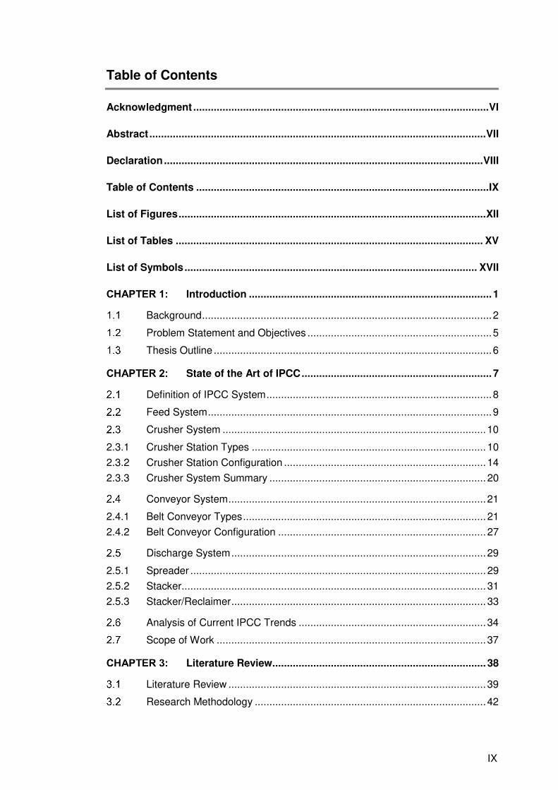
Figure 2-14 Type of crusher by decade .................................................................. 18
Figure 2-15 a) Transport crawler (Sandvik); b) SPMT [49] ...................................... 20
Figure 2-16 Fully-mobile belt conveyor a) belt wagon (Sandvik); b) bridge conveyor .............................................................................................. 22
Figure 2-17 Fully-mobile horizontal conveyor (TNT) ............................................... 23
Figure 2-18 Portable belt conveyor a) in limestone quarry (Metso); b) at heap leach; c) at waste dump (both Terra Nova Technologies) ............................... 24
Figure 2-19 Shiftable belt conveyor a) trackshifting [61]; b) drive station mounted on crawler [62]; c) at operating face [63] ................................................... 25
Figure 2-20 Relocatable belt conveyor a) overland conveyor); b) cross section (Sandvik) ............................................................................................. 25
Figure 2-21 Fixed belt conveyor a) installation in coal mine; b) to power plant; c) HAC ..................................................................................................... 26
Figure 2-22 Belt conveyor components a) exploded view [67]; b) schematic view [50] ...................................................................................................... 27
Figure 2-23 Discharge system equipment types by material and location ............... 29
Figure 2-24 Spreader a) C-frame type; b) compact type (Sandvik) ......................... 30
Figure 2-25 Cross pit spreader (Sandvik) ............................................................... 31

XIII
Figure 2-26 Stacker a) double boom on rails (Sandvik); b) extendable single boom on crawlers (TNT)................................................................................ 32
Figure 2-27 Mobile stacking conveyor [78] ............................................................. 32
Figure 2-28 Stacker/Reclaimer a) bucket wheel type b) circular type (both Sandvik) .............................................................................................. 33
Figure 2-29 IPCC installations by type.................................................................... 34
Figure 2-30 IPCC system capacities ...................................................................... 36
Figure 2-31 IPCC applications for different material types ...................................... 36
Figure 2-32 Illustration of simplified SMIPCC system ............................................. 37
Figure 4-1 Parameters influencing loader capacity adjusted after [108] ................ 48
Figure 4-2 Histogram of bucket cycle times of Volvo EC460CL ............................ 50
Figure 4-3 Bucket capacity ................................................................................... 51
Figure 4-4 Histogram of bucket payload (all cycles) of the 700t hydraulic excavator ............................................................................................ 53
Figure 4-5 Truck payload histogram ..................................................................... 54
Figure 4-6 Number of bucket cycles probability .................................................... 56
Figure 4-7 Comparison of number of bucket cycles probability ............................. 59
Figure 4-8 Single-side method (left) and double-side method (right)..................... 60
Figure 4-9 Drive-by method (left) and modified drive-by method (right) ................ 60
Figure 4-10 Truck loading scenario - Case a .......................................................... 61
Figure 4-11 Truck loading scenario - Case b .......................................................... 61
Figure 4-12 Histogram of truck loading time with two superposed normal distribution ........................................................................................... 63
Figure 4-13 Travel time distribution - data used from [133] ..................................... 65
Figure 4-14 Travel time distribution loaded (left) unloaded (right) ........................... 65
Figure 4-15 Schematic illustration of general operation process of system elements ............................................................................................. 67
Figure 4-16 Schematic illustration of simplified operation process of system elements ............................................................................................. 67
Figure 4-17 Schematic illustration of elementary operation process of system elements ............................................................................................. 68
Figure 4-18 Schematic illustration of work time of a system element ...................... 68
Figure 4-19 Element specific unplanned downtime causes .................................... 72
Figure 4-20 Repair time histogram of a crusher station .......................................... 73
Figure 5-1 Schematic illustration of simplified SMIPCC system ............................ 78
Figure 5-2 Open cut time model Xstrata [170] ...................................................... 79
Figure 5-3 Time allocation model Rio Tinto [171] ................................................. 80
Figure 5-4 Time usage model used by Western Premier Coal Limited [114]......... 80
Figure 5-5 SMIPCC time usage model ................................................................. 81
Figure 5-6 Trackshift patterns ............................................................................... 86
Figure 5-7 Schematic illustration of the SMIPCC system ...................................... 90

XIV
Figure 5-8 Simulation model flowchart .................................................................. 93
Figure 6-1 Hypothetical coal mine layout ............................................................ 102
Figure 6-2 SMIPCC system capacity for various number of trucks ...................... 105
Figure 6-3 SMIPCC system capacity change for various trucks .......................... 105
Figure 6-4 System Delay Ratios for loader and truck for various number of trucks ................................................................................................. 106
Figure 6-5 Economic analysis on OPEX ............................................................. 107
Figure 6-6 Effective operating time and system-induced operating delays of Loader, Truck and IPCC ................................................................................. 107
Figure 6-7 Sensitivity analysis on mean time to repair ........................................ 108
Figure 6-8 SMIPCC system capacity vs. stockpile capacity ................................ 109
Figure 6-9 Cost per tonne of SMIPCC system for various stockpile capacities ... 110
Figure 6-10 Reduction of SMIPCC system cost per tonne by stockpile capacity increase ............................................................................................. 111
Figure 6-11 Comparison of effective operating time and system-induced delay of the loader ................................................................................................ 112
Figure 6-12 Comparison of effective operating time and system-induced delay of the truck................................................................................................... 112
Figure 6-13 Comparison of annual system capacity and total OPEX .................... 113
Figure 6-14 Comparison of cost per tonne ............................................................ 114
Figure 6-15 Annual system capacity vs. cost per tonne ........................................ 114
Figure 6-16 Annual system capacity vs. truck quantity .......................................... 115

XV
List of Tables
Table 2-1 Main parameter of primary crushers ........................................................ 16
Table 2-2 Summary of main crusher station parameters .......................................... 21
Table 2-3 Design parameters of fully-mobile conveyors ........................................... 23
Table 2-4 Design parameters spreader .................................................................... 31
Table 2-5 Design parameters of stackers ................................................................ 33
Table 2-6 Design parameters of stacker/reclaimer ................................................... 33
Table 4-1 Summary of statistical analysis of bucket cycle times .............................. 50
Table 4-2 Summary of bucket payload data ............................................................. 53
Table 4-3 Data analysis parameters ........................................................................ 58
Table 4-4 Summary of data collection ...................................................................... 69
Table 4-5 Literature on repair time and associated distribution ................................ 71
Table 4-6 Summary of mean repair time of SMIPCC system elements .................... 74
Table 4-7 Literature on work times and associated distributions .............................. 74
Table 4-8 Summary of mean work time of SMIPCC system elements ..................... 75
Table 4-9 Summary of repair ratio values of SMIPCC system elements .................. 76
Table 5-1 Simulation input parameters .................................................................... 94
Table 5-2 Secondary simulation input parameters ................................................... 95
Table 5-3 Truck states ............................................................................................. 97
Table 5-4 Element states ........................................................................................100
Table 6-1 Loader and truck parameters ..................................................................103
Table 6-2 Disturbance parameters of SMIPCC system elements ............................104
Table 6-3 OPEX parameters for system elements ..................................................106

XVI
List of Abbreviations
CAT Caterpillar Incorporation CECE Committee of European Construction Equipment CPU Central Processing Unit CV Coefficient of Variation DIN Deutsche Industrie Norm e.g exempli gratia / for example EKG Russian Rope Shovel Type ESUM Extended Summation Method FAM Förderanlagen Magdeburg FMIPCC Fully-Mobile In-Pit Crushing and Conveying GDR German democratic republic HAC High Angle Conveyor IGD Inverse Gaussian Distribution IPCC In-Pit Crushing and Conveying MMD Mining Machinery Developments MSC Mobile Stacking Conveyor n.a not available O&K Orenstein & Koppel OPEX Operational Expenditures PVC Polyvinylchlorid SAE Society of Automotive Engineers SMIPCC Semi-Mobile In-Pit Crushing and Conveying SMU Service Meter Unit SPMT Self-Propelled Modular Transporter ST Steel (conveyor breaking strenght) TAKRAF Tagebau-Ausrüstungen, Krane, und Förderanlagen TGL Technische Normen, Gütevorschriften und Lieferbedingungen TNT Terra Nova Technologies TPMS Truck Payload Management System TU Technische Universität UB Universalbagger USA United States of America VBA Visual Basic for Application VIMS Vital Information Management System

XVII
List of Symbols
Symbol Notation Unit
a Shape parameter gamma function
Theoretical hourly capacity of discontinuous loaders t/h
Hourly capacity of discontinuous loaders t/h
Annual system capacity t/a
Hourly truck capacity t/h
Maximum acceptable truck payload t
Bucket payload t
Truck payload t
Truck payload t
Coefficient of variation
Maximum overload factor
Bucket fill factor
Material swell factor
F(x) Function value of x
g Probability density function of gamma distribution
Number of Trucks
Number of bucket cycles
P(x) Probability of x
s Scale parameter gamma function
Mean of repair time min
Mean work time min
Operating delay h
Effective operating time h/a
Truck travel time loaded s
Truck travel time unloaded s
Empty bucket swing time s

XVIII
Symbol Notation Unit
Bucket fill time s
Loaded bucket swing time s
Bucket dump time s
Blasting time h
Calendar time h
Truck cycle time s
Manoeuvre and dump time at crusher s
Downtime h
( ) Non-scheduled production h
( ) External disturbances h
( ) Preventative maintenance h
( ) Planned shift delays h
( ) Technological downtime h
( ) Technological downtime proportional to effective operating time h
( )
Technological downtime not proportional to effective operating time h
Unplanned downtime h
Bucket cycle time s
Truck loading time s
Truck loading time from the loader perspective s
Truck loading time from the truck perspective s
Operating time h
Self-induced operating delays h
System-induced operating delays h
Manoeuvre and spot time at the loader s
Conveyor trackshifting time h
Truck travel time s

XIX
Symbol Notation Unit Loader inherent wait time s
Rated bucket volume m³
blast volume m³
Maximum dump block volume m³
Expected value
X Random variable
Mean bucket payload t
Mean bucket cycle time s
Variance of bucket payload t²
Variance of bucket cycle time s²
Variance of truck travel time s²
Variance
Material insitu density t/m³
Γ(x) Gamma function
ϰ Repair ratio
μ Mean value
Technological downtime ratio
Distribution function of standard normal distribution
system delay ratio
Operating delay ratio
Pi
Probability density function of standard normal distribution


1
INTRODUCTION
This chapter presents the framework of the thesis. The main objectives and background are provided, which set the focus of the thesis.

CHAPTER 1: Introduction
2
BACKGROUND
Material transport in hard-rock surface mines, as one of the primary technological
processes, is comprised of all tasks necessary to transfer excavated material from the
working face to the dump area, the processing plant or to subsequent treatment areas.
This task is accomplished by employing appropriate technical means which are able to
receive, transport and discharge excavated material according to operational
requirements [1].
Today´s predominant means of material transport in hard-rock surface mines are
conventional mining trucks. The reasons for this development are based on inherent
advantages of conventional mining trucks which are able to carry out the majority of
the technological processes, i.e. intake of material at loading point inside pit, transport
and discharge to the final destination out of pit. They are furthermore well established,
provide high reliability, excellent flexibility with regards to pit geometry and production
rate, and sufficiently satisfy the needs for material blending. Conventional mining trucks
also provide the mine owner with the choice of either owning and operating the mining
fleet, or engaging a contactor to supply and manage the fleet. Lastly, conventional
mining trucks allow flexible production assignments by simple up or down scaling of
the truck fleet.
However, when analysing today´s situation in hard-rock surface mines under techno-
economic aspects in comparison to the situation during 1970 and 2010, it must be
noted that material transportation cost as part of the overall mining cost could not be
reduced, despite rationalizing efforts mainly through introduction of more productive
mining trucks. During 1970 and 2008 the average payload of mining trucks used in
surface mines doubled from 90 t to just over 180 t [2] while the current maximum
payloads reach 450 t [3]. On the contrary, material transportation cost increased
significantly while facing a simultaneous and substantial increase of the overall mining
cost. Some authors [4], [5] estimate transport cost shares between 40 to 50% while
others even suggest costs up to 60% of overall mining cost [6], [7].
The primary reasons for these developments are:
• Constant declining head grades of ore. During the last decades, the average
grade of the main hard-rock commodities has declined substantially. Figure 1-1
indicates the general trend for various hard-rock commodities over the last
century.

1.1 Background
3
Figure 1-1 Decreasing head grades of various metals [8]
• Declining ore grades directly translates into an increase of material movements.
Figure 1-2 indicates the development of stripping ratios of the main hard-rock
commodities over the last decades. Particularly in the last 20 years the stripping
ratios have doubled or even tripled.
Figure 1-2 Increasing waste rock to ore ratio [8]
• And furthermore, increasing depth of mineral deposits which directly translates
into rising horizontal and especially vertical transport distances. Figure 1-3
indicates the development of mineralization depth of copper deposits over the
last decades. For example, by 2000 the average depth of mineral discovery
reached 295 m in Australia, Canada and USA.

CHAPTER 1: Introduction
4
Figure 1-3 Average depth of newly discovered ore deposits [2]
• And lastly, the mining industry´s reluctance and risk adhesiveness to adopt new
technology.
In the light of these statements, it can be concluded that:
• In terms of costs, the technological processes drilling, blasting and loading
increasingly lose importance on account of material transportation.
• Should conventional mining trucks, in their current development stage, continue to
be utilised for the majority of material transport in hard-rock mines, then it is to be
expected that overall mining cost will continue to face a significant increase.
• Material transportation represents one of the biggest operational cost in mining
and with the drive towards higher productivity, lower capital and operational
expenditures it also represents an area where the greatest impact can be made.
Thus, considerations and efforts to reduce overall mining costs, promises highest
success when focusing on the development, testing and utilization of more economic
material transport methods. Developments which enable hard-rock surface mines to
transport material more environmentally sensibly, more safely and at lower cost should
therefore be seen as a main task for the future in the mining sector.
Conveyor haulage, as a well-known continuous transportation method in soft-rock
mines, represents a viable, safer and less fossil fuel dependent alternative [9]. Around
40% of the total energy used in hard rock surface mines is related to diesel
consumption, and truck haulage is responsible for the majority of this diesel
consumption, which is the primary source of CO2 emissions.
The essential criterion for the application of conveyor haulage in hard rock surface
mines is the availability of a conveyable bulk mass. At the moment, crushing represents
the only safe and applicable process for this criterion and can be seen as an
intermediate process between the main technological processes excavation and
transportation. This material transportation method is known as an in-pit crushing and
conveying system (IPCC).

1.2 Problem Statement and Objectives
5
PROBLEM STATEMENT AND OBJECTIVES
The material transport by IPCC systems in hard rock surface mines is not a new
technology. Already in 1956 the first self-propelled crusher connected to conveyors
was installed in the limestone quarry Höver, Germany [10], [11]. The use of these early
installations was not driven by economic reasons but rather to overcome major
problems regarding wet and soft ground conditions which did not allow the use of trucks
[12].
In the last decade, the mining industry has developed particular interest in IPCC
systems for the transportation of waste material. The growing interest is mainly driven
by inherent system advantages regarding operating cost, environmental health &
safety as well as operational & planning considerations [13]. However, one of the
mentioned drawbacks of IPCC systems is the inability to project reliable long term
system capacity [14]–[17].
As the interest for IPCC systems increases so does the demand for investigative
studies. Increasingly a standard procedure of mining companies to compare
productivity and the profitability of conventional truck haulage and IPCC transportation
methods in the early stages of a new mining project [18]. Sandvik Mining a business
unit within the Sandvik Group, faces this demand and provides technical mining studies
with comparisons in desktop, scoping and engineering design level.
Additionally, the interest in this material transport method is also reflected by the
increasing amount of scientific studies [19]–[22]. Many of them have proven the
economic advantageousness of IPCC systems compared to conventional truck and
shovel operation. The emphasis of their examination lies in the area of operating cost
and capital expenditure.
The groundwork for such investigative studies as well as for economic comparisons is
the knowledge of achievable effective operating hours of these systems and their
corresponding annual capacity to meet assigned production schedules. Historically,
deterministic calculations based on empirical data adopting mean values as inputs,
tempered with intuition and refined with engineering judgment provided merely
satisfactory estimates of effective operating hours and corresponding annual capacity.
However, disturbances and variations such as delays and hold-ups are inevitable in
any earthmoving, quarrying and mining operation no matter how well the operation may
be planned or managed [23], [24]. Thus, all too often such traditional calculation
methods have proven to be unattainable in practice and outcomes have not met
expectancy. Furthermore, all previously mentioned authors assumed a fixed annual
IPCC system capacity based on deterministic methods and engineering judgment for
their comparisons which has four notable shortcomings; they

CHAPTER 1: Introduction
6
1. underestimate the influence of the random behaviour of system components
and their interactions,
2. are time consuming when alteration is necessary to suit individual project
requirements,
3. lack in terms of standardization throughout the industry, and
4. systematically carry hazards of human error and under or overestimate the
achievable IPCC system capacities.
Therefore, the objective of this thesis is to develop a structured method which allows
the estimation of the annual capacity of IPCC systems under consideration of the
random behaviour of system elements and their interactions with one another. Hence
a research project was initiated by Sandvik Mining in cooperation with the Institute of
Mining of the Freiberg University of Mining and Technology in this area, which is the
subject of the work presented in this thesis.
THESIS OUTLINE
Following the introduction, chapter 2 discusses the current state of the art of IPCC
system. The chapter provides a general definition of IPCC systems, describes the
technical function of all sub-systems of an IPCC systems and analyses the current
trends. This chapter further defines the scope of work.
Chapter 3 provides a literature review of previous studies and methods related to IPCC
system capacity determination. It focuses on those studies and methods which
emphasise semi-mobile IPCC (SMIPCC) systems. The purpose of this task is to reveal
the current available methods and their disadvantages for capacity determination of
SMIPCC systems.
Chapter 4 provides a comprehensive statistical analysis of the random behaviour of
the SMIPCC system elements to quantify capacity and disturbance variation. The
analysis is based on operational data from various mine sites obtained by the author.
Chapter 5 describes the proposed method for the estimation of the annual capacity of
IPCC systems. Furthermore, chapter 5 describes the stochastic simulation model to
determine the system delay ratio.
In chapter 6 the method is used in a case study to analysis the system behaviour based
on a hypothetical mine with regards to time usage model component, system capacity,
and cost as a function of truck quantity and stockpile capacity. Furthermore, a
comparison between a conventional truck & shovel system and SMIPCC system is
provided.
Lastly chapter 7 summarizes the main findings of this research and provides
suggestions and ideas for further research.

7
STATE OF THE ART OF IPCC
This chapter provides a general definition of the term IPCC system by dividing it into sub-systems. Each sub-system is then described in detail and general capacity limitations are provided. The chapter concludes with an analysis of the currently installed IPCC systems and presents the general development and trends.

CHAPTER 2: State of the Art of IPCC
8
DEFINITION OF IPCC SYSTEM
In a narrow sense, IPCC systems can be defined as continuous haulage systems for
surface mines, which are comprised of a crusher system (one or multiple crusher
stations), located inside the pit, combined with a conveyor system for the purpose of
transporting material out of the pit. In a broader sense an IPCC system can be defined
as an integrated bulk material handling systems that consists of
• a feed system,
• a crusher system,
• a conveyor system, and
• a discharge system which
represents a combination of discontinuous excavation & loading as well as continuous
transport & discharge1. Figure 2-1 illustrates the process flow of an IPCC system.
Figure 2-1 IPCC system process flow
Atkinson (1992) differentiates in [25] IPCC systems based on the mobility of the
crushing station into mobile, semi-mobile, movable, modular, semi-fixed and fixed.
Today, the mining industry simplifies the differentiation into fixed, semi-mobile and fully-
mobile IPCC system [14], [26]. In this thesis, the common industry terminology is
adapted and further substantiated by semi-fixed systems to better distinguish the range
of mobility among IPCC systems.
A survey conducted by the author, on in-pit crusher station population according to the
aforementioned definition revealed that 447 in-pit crusher stations have been installed,
are currently in erection/manufacturing process or on order since 1956. Reference data
provided by the leading IPCC equipment manufacturers including (in alphabetical
order) Förderanlagen Magdeburg (FAM), FLSmidth, Hazemag, JoyGlobal, Metso,
Mining Machinery Developments (MMD), Sandvik, Tenova TAKRAF and
ThyssenKrupp2 served as a basis of the survey. A detailed list of all IPCC references
can be found in Appendix I. Figure 2-2 shows the distribution of in-pit crusher stations
by region. The pie charts indicate the distribution of crusher station type and the total
1 Hereinafter IPCC refers to the entire material handling system from winning to discharge operation. 2 including Weserhütte, O&K and PHB Fördertechnik

2.2 Feed System
9
number of crusher stations since 1956. The black marks point out the area of in-pit
crusher stations utilised for large mining operations since 1970.
Figure 2-2 In-pit crusher station distribution by region and type
The majority of IPCC systems were installed in Europe, mainly during the 1960s
throughout the 1990s. The systems were predominantly fully-mobile and installed in
limestone quarries. However, due to stagnating mining activities in the following
decades Europe became less active with regards to IPCC system installations.
Increasing IPCC operations of semi-mobile and semi-fixed type started in the 1980s
throughout 2000 in North America in copper and gold deposits. In recent years, Central
Asia (including China, India and Thailand) and South America have become key
regions for IPCC installations, due to major green field and expansion projects for iron
ore in South America and for coal projects in Central Asia.
FEED SYSTEM
The feed systems function is to excavate the material from the operating face and feed
the crusher system. It can be divided into cyclic excavation and cyclic intermittent
haulage. Depending on the type of in-pit crusher the feed system may consist of a
single piece of equipment or a combination of multiple.
In an IPCC system, typical equipment for the excavation process are rope shovels,
hydraulic excavators and front end loader. In some cases, dozers and draglines are
used to excavate material and directly load the crusher station1. Possible equipment
combinations with respect to in-pit crusher type are shown in Figure 2-3.
1 E.g. Gravel pit in Milford, Iowa; Oliver Iron Mining Company in Hibbing, Minnesota

CHAPTER 2: State of the Art of IPCC
10
Figure 2-3 Feed system combinations
Fully-mobile crusher stations are commonly fed directly by cyclic unit loaders such as
electric rope shovels or hydraulic excavators. Combinations of front end loaders (in
load and carry operation), dozers (in dozer push operation), draglines and fully-mobile
crusher stations are possible but are more common with semi-mobile crusher stations1
[27], [28]. The feed system of fixed and semi-fixed crusher stations is typically indirect
and consists of electric rope shovels, hydraulic excavators or front-end loaders in
combination with mining trucks. In some cases, trains are also used for intermittent
haulage2.
CRUSHER SYSTEM
The crusher systems function, regardless of the type, is to receive material from feed
system, comminute the material to a conveyable size and discharge it onto the
conveyor system.
2.3.1 Crusher Station Types
The following definitions were established to categorize in-pit crusher stations by the
degree of mobility, structural design and location of operation into:
• fully-mobile
• semi-mobile
• semi-fixed (modular and non-modular), and
1 E.g. Drummonds coal Ceasar mine, Columbia – Dozer push operation 2 E.g. ArcelorMittal´s Iron ore mine at Krivoy Rog, Ukraine

2.3 Crusher System
11
• fixed.
Fully-Mobile In-Pit Crusher Station
Fully-mobile crusher stations (Figure 2-4) have, analogous to the term, the ability to
change position (follow the operating face) by system integrated transport
mechanisms. They are directly fed by a single loading machine and move in unison
along the operating face. Loading by multiple machines is possible but has been
proven to be impractical [29]. Although most crusher stations with crawler track support
are labelled as “fully-mobile”, only a few are actually able to follow the movements of
the loader continuously. Most fully-mobile crusher station designs require the hopper
of the crusher station to empty before a movement can commence. This in turn leads
to significant operating delays of the loading unit.
Figure 2-4 Fully-mobile crusher stations for mining operation (left) for quarry operation (right)
[30]
Semi-Mobile In-Pit Crusher Station
Semi-mobile crusher stations (Figure 2-5) are machines without system integrated
transport mechanisms which are commonly located at operating level and allow
multiple loading machines (commonly front end loaders) to feed the material from
various loading points. Relocation is realized within several hours by transport crawlers
or dozers without disassembly and planning efforts whenever the distance reaches the
economic limit.
Figure 2-5 Semi-mobile in-pit crusher station a) with transport crawler for relocation [31]; b)
skid mounted loaded by front end loader in coal mine [32]

CHAPTER 2: State of the Art of IPCC
12
Semi-Fixed In-Pit Crushing Station
Semi-fixed crusher stations are machines without system integrated transport
mechanisms, which are commonly located at strategic junction points within the pit and
fed by mining trucks from multiple operating levels and loading points. They are further
differentiated into modular and non-modular crusher stations. The design criterion of
modular in-pit crusher stations is to relocate to new locations quickly without major
disassembly and erection costs whenever multiple relocations are intended. Both types
can be designed as direct dump (Figure 2-7) or indirect dump stations (Figure 2-6)
depending on the existence of an integrated feed system (e.g. apron feeder).
Relocation requires disassembly of the entire crusher station into several parts or into
multiple (2 to 6) modules and is realized by transport crawlers or self-propelled modular
transporters. The relocation process takes several days for modularised semi-fixed
crusher stations and several weeks up to one month for stations that are not
modularised depending on the type of civil works required for ground and wall
preparation.
Figure 2-6 Semi-fixed modular indirect dump in-pit crusher station a); with gyratory crusher b)
with double roll crusher (both Sandvik)

2.3 Crusher System
13
Figure 2-7 Semi-fixed non-modular direct dump crusher station with gyratory crusher [33]
Fixed In-Pit Crusher Station
Fixed crusher stations (Figure 2-8) are commonly located near the pit rim or at a
position inside the pit that is not affected by mining activities. They are typically
designed to operate at one place for the entire life of mine and are not intended to
relocate. The two common designs are either in-ground (e.g. Dexing copper mine,)
China) or rim mounted (e.g. Cananea copper mine, Mexico). In both designs, the
crusher is installed in a concrete structure with some steel portions.
Figure 2-8 Fixed in-pit crusher station a) concrete structure [33]; b) steel structure [34]

CHAPTER 2: State of the Art of IPCC
14
2.3.2 Crusher Station Configuration
In-pit crusher stations are composed of multiple subsystems including:
• material charge,
• integrated material feed system,
• crusher,
• integrated material discharge system,
• auxiliary systems,
• framework, and
• substructure/undercarriage.
Subsystem – Material Charge
The subsystem material charge has, depending on the loading process and the
successive subsystems, the following functions:
• to balance and buffer the inevitable fluctuation of material flow by the
discontinuous loading process,
• to protect the feeding system from impact and wear damage, and
• to shorten the loading cycle time though simplified discharge procedure of the
loading machine.
In current designs material charge is commonly realised by a hopper without an
additional discharge mechanism. Charging troughs are less common and only applied
to small capacity crusher station. The material charge system capacity is subject to the
unit capacity of the loading/feeding device. Plattner [35] and Kirk [36] suggest a
minimum factor of 1.5 (unit capacity to hopper capacity). More contemporary
information advise a factor of 2 - 3 [37].
Subsystem – Material Feed System
The function of the material feed system is to evenly withdraw material from the
material charge and to control the rate the material enters the crusher. Today, crusher
station designs commonly use rigid apron feeders as their material feed system. They
are built with a series of linked steel plates connected to electric motor driven steel
chains. Apron feeders have demonstrated reliable performance when handling large
sized blocks and material with high deviation in feed size distribution and moisture
content. Other feed systems include chain feeder, belt feeder, vibrating feeder, and
grizzly feeder. Apron feeders can be built with an inclination of up to 30° as in contrary
to belt feeders with a maximum inclination of 18°. This reduces the length at equal
lifting height by 60%. However, apron feeders have a high service weight, are capital
intensive and require frequent maintenance.

2.3 Crusher System
15
The selection of the material feed system depends on the material properties, the
fragmentation size, crusher type and capacity requirements. In-pit crusher station
without material feed systems are referred to as direct dumping stations.
Subsystem – Crusher
The crusher subsystem is, based on its primary function which is to reduce the material
to a conveyable size, a central component of an in-pit crushing station. The following
crusher types are used in IPCC systems:
• Feeder breaker • Jaw crusher • Gyratory crusher • Roll crusher • Hybrid crusher • Sizer • Impact crusher
•
Principles and experiences that are valid for the selection of crushers in conventional
crusher stations can also be applied for in-pit crushing stations. However, attention is
required for the selection of crushers with regards to the overall concept of in-pit
crushers. Service weight, design dimensions, and resulting dynamic stresses need to
be accounted for. The following criteria need to be considered for the crusher selection:
• Material properties (density, moisture, hardness, stickiness, abrasiveness).
• Application requirements (feed size, product size, product size distribution,
content of fines, capacity).
Figure 2-9 and Table 2-1 show the main parameters of the aforementioned crushers
used for in-pit crusher stations. All parameters are based on data from [38]–[47].
Figure 2-9 Range of application for crusher types by material compressive strength and
capacity

CHAPTER 2: State of the Art of IPCC
16
The graph indicates the maximum values for capacity and compressive strength of
material. It must be noted that the crusher throughput is also a function of the reduction
ratio between material feed size and required final product size.
Table 2-1 Main parameter of primary crushers
The main selection parameters including achievable capacity, maximum feed size,
achievable reduction ratio and material compressive strength of primary crushers are
illustrated in Figure 2-10 to Figure 2-13.
Figure 2-10 Crusher selection by capacity

2.3 Crusher System
17
Figure 2-11 Crusher selection by feed size
Figure 2-12 Crusher selection by reduction ratio
Figure 2-13 Crusher selection by compressive strength of material
An analysis of utilisation of the different crusher types since 1960 is illustrated in Figure
2-14.
CHAPTER 2: State of the Art of IPCC
18
Figure 2-14 Type of crusher by decade
For industrial or mass commodities including limestone, dolomite, diorite, granite,
marble, and basalt the impact crusher represents the most widely used crusher type
(50%). This might be justified by the fact that in this industry the crusher serves an
additional function which is to produce a product size and shape that can be directly
fed to the processing plant (maximum reduction ratio of 1:50 and above can be
achieved). Additionally, impact crushers are capable of crushing rock with a moisture
content up to 10%. In recent years, jaw crushers with pre-screens and sizers have
been increasingly used.
In copper and gold deposits the gyratory crusher is the main crusher type (86%). This
dominance may be explained by the crusher’s ability to process material with high
compressive strength in high capacities.
The main crusher types for coal and oil sand deposits are double roll crusher and sizer
with a share of 54 and 26%, respectively. They are able to process wet and sticky
material at high capacity rates.
Iron ore deposits employ mainly gyratory crushers (39%) for the same reason as for
copper and gold deposits. Recently, jaw (24%) and hybrid crushers have been
frequently utilised especially in combination with fully-mobile crusher stations. Hybrid
crusher feature a compact design (>40% size reduction compared to double roll
crusher), generate a minimum of undesirable fines and are able to process material up
to 300 MPa.
Subsystem – Material Discharge
The purpose of the material discharge system is to release and guide the crushed
material to the subsequent element. Fixed and semi-fixed crusher stations use
overlapping flight apron feeders, vibrating feeder, belt conveyor or outlet chutes as their

2.3 Crusher System
19
discharge system. Fully-mobile stations may have a slewable and/or luffable belt
conveyor directly attached, or have outlet chutes.
Subsystem – Auxiliary Systems
Auxiliary systems include all systems that are required if additional tasks are
necessary. For instance, pre-screening devices (located in the material feed systems)
which allow smaller material to bypass the crusher, therefore minimising the amount of
material to be crushed and increasing the overall throughput. Other auxiliary systems
include service cranes, rock breakers, control room, spillage chute, truck-bridge, and
magnetic separators.
Subsystem – Framework
The framework has the function of connecting all subsystems. Fixed crusher stations
(in-ground or rim mounted) commonly have a concrete structure with some portion of
fabricated steel. Semi-fixed, semi-mobile and fully-mobile crusher stations are
mounted on a steel structure.
Subsystem – Substructure
The substructure is the lower-most part of the crusher station which supports and
evenly transmits static and dynamic loads occurring in the station to the bearing ground
surface. A fixed crusher station’s substructure is made of concrete, whereas semi-fixed
and semi-mobile crusher stations are commonly supported by steel footers. In most
cases, simply a bed of compacted gravel is required to ensure an appropriate
foundation for steel footers.
The substructure, or in this case undercarriage, of fully-mobile crushing stations serves
an additional function which is to realize required movements during the course of the
face advancement. Varying fields of application require different mobility of the fully-
mobile crusher stations. The type of transport mechanism chosen depends on the
frequency of relocation, the service weight, the prevailing operation and ground
conditions and the installation costs. Possible integrated transportation mechanisms
are:
• tires,
• hydraulic walking pads, and
• crawler tracks.
The first tire mounted fully-mobile crusher stations were introduced during the 1970s
and increased the mobility compared to crawler tracks and particularly hydraulic
walking pads. The main disadvantage is the specific ground pressure which results
from comparatively small contact surface. Tire systems are commonly used for crusher
stations with service weights up to 745 t. Hydraulic walking pads have the advantage
of high manoeuvrability; they can travel in all directions without difficulty. However, with

CHAPTER 2: State of the Art of IPCC
20
regards to travel speeds and operational availability they are inferior. Crawler tracks
are the most common transport mechanism for large fully-mobile crusher stations.
They are well suited to work in line with electrical rope shovels or hydraulic excavators
as the time and speed required to move is similar. Crawler tracks have low ground
pressure and enable a smooth and quick relocation without the necessity to shut down
the crusher. The drawbacks are high service weights and the associated capital and
maintenance costs. They are usually used in stations with higher service weights or
where ground conditions require low ground pressure. Fully-mobile crusher stations
with crawler tracks achieve travel speeds between 8 – 12 m/min for large stations and
17 - 20 m/min for smaller stations. The service weight of the station and the ground
conditions determine the number of tack rollers and the permissible ground pressure
determines width and length of the base plates.
Relocation of semi-mobile and semi-fixed crusher stations is realised with transport
crawlers or self-propelled modular transporter (SPMT) (Figure 2-15). Transport
crawlers are autonomous crawler tracks, which are able to carry loads up to 1,500 t on
a maximum gradient of 10%. They can be equipped with or without an operator’s cabin.
A self-propelled modular transporter is a platform vehicle with a large array of wheels
which can be combined to transport objects. They individually achieve maximum
transport loads up to 216.5 t with a maximum gradient of 12% [48]. Both transport
machines are equipped with electronic control systems which regulate hydraulic
cylinders to keep the load level even on rough terrain and steep gradients.
Figure 2-15 a) Transport crawler (Sandvik); b) SPMT [49]
2.3.3 Crusher System Summary
Table 2-2 summarizes and complements characteristics of the different crusher types.
It can be determined that each crusher type holds advantages under certain
parameters.

2.4 Conveyor System
21
Table 2-2 Summary of main crusher station parameters
CONVEYOR SYSTEM
In surface mining operations, the term conveyor system is used to refer to an
arrangement of belt conveyors which are selected and connected in a way that they
facilitate the transport of material out of the pit (ex-pit dump, stockyard or leach pad) or
within the pit (in-pit dump) from the crusher system to the disposal system in
compliance with the mining conditions [50]. Belt conveyors are continuous conveyors
and consist of an endless belt which runs around the drive pulley (head station) and
idler pulley (tail station) and can be driven by one or multiple drive pulleys using static
friction. Between the pulleys the belt is supported by load bearing idlers. The required
belt tension is controlled by the tension system. The material is commonly charged
onto the conveyor in proximity to the tail station using a loading hopper and transported
on top of the belt to the head station where it is discharged.
2.4.1 Belt Conveyor Types
Just like crusher stations, belt conveyors can be classified by the degree of mobility,
structural design and location of operation into:
• fully-mobile,
• portable,
• shiftable,
• semi-fixed, and
• fixed belt conveyors.
The following section describes various types of belt conveyors, their components and
application. It furthermore focuses on troughed belt conveyors; other belt conveyors
types that also find application in surface mines such as cable belt conveyors, air
supported belts, suspended belt conveyors and enclosed belt conveyors are not
explained but information can be found in [51]–[53].

CHAPTER 2: State of the Art of IPCC
22
Fully-Mobile Belt Conveyors
Fully-mobile belt conveyors have the ability to change position by system integrated
transport mechanisms (almost exclusively with crawler tracks). All components as
described in section 2.4.2 are integrated in the structure. Fully-mobile belt conveyors
are typically associated with fully-mobile IPCC systems where they are utilised as a
link between fully-mobile crusher and shiftable conveyor at the operating face.
Additionally, the following secondary functions are realised by fully-mobile conveyors:
• to allow multiple block and bench operation, and
• to increase the overall block width and block height.
Thus the production time between two shifting operations of a shiftable conveyor
increases which results in a higher utilisation of the entire material handling systems.
There are two main fully-mobile belt conveyors types (Figure 2-16) which are
applicable in IPCC operations:
• belt wagons, and
• bridge conveyors.
Belt wagons may also be built semi-mobile and are relocated by transport crawlers
(e.g. Yimin He coal mine, China).
The main difference with regards to design between the types is the number of crawler
track sets and the boom construction. Belt wagons commonly use a single crawler
track set which is connected to the superstructure including independently luffable and
slewable receiving and discharge boom. Bridge conveyors use two sets of crawler
tracks which support the receiving and discharge side of a single boom.
Figure 2-16 Fully-mobile belt conveyor a) belt wagon (Sandvik); b) bridge conveyor

2.4 Conveyor System
23
An additional type of fully-mobile belt conveyors are fully-mobile horizontal conveyors
(Figure 2-17). They are levelled conveyors which have a receiving hopper over the full
length. They are located at the dump or heap leach pad.
Figure 2-17 Fully-mobile horizontal conveyor (TNT)
Table 2-3 summarizes the technical parameter of fully-mobile belt conveyor. All
parameters provided are based on data from [54]–[57]
Table 2-3 Design parameters of fully-mobile conveyors
Parameter Belt Wagon Conveyor Bridge Horizontal Conveyor
Max. receiving boom length [m]
50 150 87
Max. discharge boom length [m]
50
Max. capacity [loose m³/h] 10,000 20,000 4,000
Belt width [mm] 2,500 2,800 1,600
Service weight [t] 550 300 -
Portable Belt Conveyors
The portable belt conveyors (Figure 2-18), also referred to as grasshoppers, are
inclined conveyors with a maximum length of 42 m comprised of a tail skid and a set
of non-powered tires located near the balance point. Designs may include crawler
tracks which are self-propelled. All components as described in section 2.4.1 are
integrated in the structure. Their function is to link a fully-mobile in-pit crusher station
at the operating face to a further stage in the conveyor system [58]. Another purpose
of portable conveyors is to transport material at the downstream end of the system
across active dump/heap areas where they are connected to a radial stacker. They are
able to follow the crusher station as it moves along the operating face, and can be
moved by the crusher station itself or other mobile equipment to a safe distance for
blasting. Each conveyor can be moved individually or in combination of two or three
units. Maximum capacities of 3,000 t/h are achieved with 1,600 mm belts and 28 t
service weight [59], [60].

CHAPTER 2: State of the Art of IPCC
24
Figure 2-18 Portable belt conveyor a) in limestone quarry (Metso); b) at heap leach; c) at
waste dump (both Terra Nova Technologies)
Shiftable Belt Conveyors
Shiftable belt conveyors (Figure 2-19) comprise of 4 - 6 m long portable conveyor
modules spaced along their longitudinal axis. The modules are mounted on steel
sleepers and consist of steel frames that hold the carrying and return roller. Steel rails
are connected to the steel sleepers to maintain a predetermined spacing between the
modules. The steel rails allow the shiftable conveyor to be moved without dismantling
in lateral direction by pipe laying dozers with a trackshifting head. The dozer engages
the conveyor and applies lateral shifting forces to bend the conveyor. Shiftable
conveyors are located either inside the pit parallel to the operating face or at the dump
face. They are moved periodically to follow the operating face advance or dump
advance. Shiftable belt conveyors are usually associated with mobile or semi-mobile
drive stations mounted on steel pontoon, steel sleepers or crawlers. The following three
shifting patterns are possible: parallel shifting in which all modules of the shiftable
conveyor are shifted over the same distance; radial shifting where one end (head or
tail end) of the shiftable conveyor remains in the same position and functions as a pivot
point while the other end is swung around this end; and combined shifting which uses
both shifting techniques parallel and radial in a way that one end of the conveyor is
shifted further than the other. The shifting process time depends on ground conditions,
conveyor length, shifting width and available work and equipment force. It typically
takes between 8 - 24 h and is split up into 3 processes including preparation for shifting,
shifting process, and alignment & start-up process.

2.4 Conveyor System
25
Figure 2-19 Shiftable belt conveyor a) trackshifting [61]; b) drive station mounted on crawler
[62]; c) at operating face [63]
Semi-Fixed Belt Conveyors
Semi-fixed or relocatable belt conveyors (Figure 2-20) are wherever infrequent
relocation or extension/shortenings are necessary such as on ramps or tunnels for pit
exit, or as overland conveyors. They consist of 4 – 6 m long portable conveyor modules
spaced along the longitudinal axis of the conveyor. The modules are mounted on
concrete sleepers and consist of steel frames that hold the carrying and return roller.
Prior to relocation the entire conveyor needs to be dismantled and each segment
carried to a different position. They are usually associated with semi-mobile or fixed
drive stations mounted on steel or concrete pontoons.
Figure 2-20 Relocatable belt conveyor a) overland conveyor); b) cross section (Sandvik)
Fixed Belt Conveyors
Fixed belt conveyors are used whenever relocation is not required during the life of
mine. Fixed belt conveyors can take on many different design forms. They are usually
located ex-pit as overland conveyors to overcome difficult terrain, and usually
associated with fixed drive stations mounted with concrete foundations.

CHAPTER 2: State of the Art of IPCC
26
High angle conveyors (HAC) and conveyor distribution points represent a special type
of fixed belt conveyors.
HAC are designed to overcome the conventional conveying angle limitations of 20°.
HAC are designed in various forms to transport material out of the pit by the shortest
distance via the pit wall. HAC designs exist with crawler tracks mounted on receiving
and discharge side to follow the advance of a heap leach dump. They use a sandwich
belt approach which employs two conventional rubber belts. The belts sandwich the
material and provide additional friction between material-to-belt and material-to-
material interface to avoid back sliding of material [64]. The HAC structure is anchored
to the mine slope and is mounted on concrete footings. The biggest installation in
surface mining operation was installed 1992 in Majdanpek copper mine (former
Yugoslavia), had belt width of 2000 mm, a capacity of 4.000 t/h at a conveying angle
of 35.5° and realised 93.5 m elevation height. Although they realise the shortest
distance possible, they are limited to a rock size of 250 mm and require a certain size
distribution [65], [66].
Conveyor distribution points, also referred to as mass distributer, are used whenever
different material are transported with a conveyor system. They provide the ability to
route material to different destinations by the use of shifting heads.
Figure 2-21 Fixed belt conveyor a) installation in coal mine; b) to power plant; c) HAC1
1 Photo taken by Karl Ingmarson – Sandvik at Vale Carajas N2 pit iron ore mine
2.4 Conveyor System
27
2.4.2 Belt Conveyor Configuration
General Components
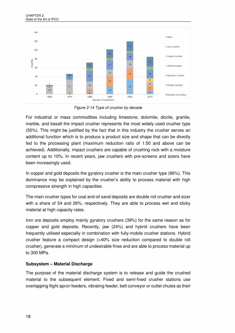
The essential components of a belt conveyor displayed in Figure 2-22 are the following
[67]:
• Drive station including drive pulley (1) with rubber or ceramic lining, bearings,
with or without transmission, electrical motor with or without coupling
• Deflection pulley (2) to increase friction angle
• Return rollers (3)
• Supporting structure (4) made of fabricated steel profiles, which sustains the
load bearing rollers
• Return pulley with tension system (5) including take-up pulleys (spindle-nut
system or gravity take-up)
• Loading hopper (6) with drop zone pads (7)
• Troughed load bearing rollers (8), commonly three or four are connected to a
garland
• Guide rolls
• Conveyor belt (9)
• Discharge with discharge chute if necessary (discharge chute requires wear
resistant lining)
• Belt cleaners and scrapers (10)
• Safety facilities such as pull-rope, rotational speed monitors, belt misalignment
switches and belt cut registration
Figure 2-22 Belt conveyor components a) exploded view [67]; b) schematic view [50]

CHAPTER 2: State of the Art of IPCC
28
Head and Tail Station
The head station (most commonly the drive station) essentially consists of the drive
pulley, with rubber or ceramic lining, and the electrical motor with or without coupling
supported by a steel structure. The drive of the head station may consist of one or
multiple drive units. They are differentiated into mobile, semi-mobile and fixed stations
depending on the frequency and the way of relocation. The installed drive capacity
covers a range from 2 times 160 kW to 6 times 2,000 kW with service weights up to
2,000 t [68], [69]. Mobile and semi-mobile stations are mounted on steel pontoons,
hydraulic walking pads or crawler tracks and are tied down by earth anchoring for quick
relocation. Fixed drive stations usually have concrete foundations and do not require
any anchoring.
Tail stations consists of the return pulley incorporated into the steel structure.
Whenever additional drive force is required they may be equipped with an electric
motor to drive the return pulley. Just like head stations they are either mobile, semi-
mobile and fixed stations. As they are considerably lighter than head stations, they are
usually mounted on steel pontoons and can be dragged by a dozer. At the operating
or dump face they may also be mounted on crawlers for quicker relocation.
Conveyor Belt
The conveyor belt is the most important component of a belt conveyor. Their function
is to receive crushed material and to transport it longitudinally. The belt requires
sufficient tensile strength in longitudinal and lateral direction, resistance against impact
energy at the loading point, and to withstand temperature and chemical effects, without
losing elasticity to adapt to the troughed structure of the carrying idlers. They are
therefore built in multiple layers comprised of pulley side cover, carcass, and carrying
side cover framed by full rubber edges.
The pulley and carrying side cover are made of smooth rubber or PVC. The carrying
side cover may also include profiles, cleats, or corrugated edges for inclined conveyors.
The carrying side is up to 3 times thicker than the pulley side for wear and impact
protection. Stresses and strains are absorbed in the centre of the belt by the carcass.
The carcass may be reinforced by textile ply (polyester, polyamide or aramid) or steel
cords and are manufactured in single or multilayers.
Belt width and tension are standardised by the manufacturers. Currently, belt widths in
the range of 800 to 3,200 mm are utilised in the surface mining industry. Belt tension
rating ranges between ST 1,000 to ST 10,000 [70]. The belt breaking strength rating
stands for the amount of pulling force that belt is able to withstand and is measured in
N/mm.
The connection of belts is accomplished either mechanically or by vulcanisation
process. Vulcanisation (hot or cold) is most commonly used in the mining industry. In

2.5 Discharge System
29
a hot vulcanisation process the reinforcements are spliced in a certain pattern, then
splices are heated and cured under pressure with a vulcanising press. Cold
vulcanisation uses a bonding agent which causes a chemical reaction to splice the two
belt ends together [71]. Vulcanisation requires a 24 h setting period. For this reason,
the frequency of belt extensions/shortenings should be minimized in a FMIPCC
operation.
DISCHARGE SYSTEM
The discharge system represents the last element of an IPCC system. Its function is to
continuously unload the material from the conveyor system in an orderly and efficient
manner to its final destination (waste dump) or to an intermediate storage location
(heap leach pad, stockyard). Discharge system equipment (Figure 2-23) can be
distinguished by the type of material discharged and the associated location of
operation into:
• spreaders,
• stackers, and
• stackers/reclaimers.
Spreaders operate at the dump site and are utilised for overburden and waste material.
Stackers handle low grade ore at heap leach pads or stack ore/coal material at
stockyards. Stackers/reclaimers are machines for unloading material onto storage piles
and reclaiming when required.
Figure 2-23 Discharge system equipment types by material and location
2.5.1 Spreader
Spreaders are mobile continuous operating discharge machines. The functions of a
spreader within an IPCC system are to receive overburden material from a tripper car
and to discharge it in a stable manner on a high or low cast dump with a certain degree
of compaction. While discharging, the spreader travels on its self-made working level
which usually has a lower ground bearing pressure than the surrounding bedrock
capacity [72].
Contemporary conveyor belt spreaders designs can be categorized by their
constructional design into compact type and C-frame type spreader (Figure 2-24). The
main difference between the two types is the counter weight arrangement. The counter

CHAPTER 2: State of the Art of IPCC
30
weight of the compact type spreader is attached below the receiving boom, allowing it
to create flatter final dump slopes by operating on a sublevel below the shiftable
conveyor, whereas the counter weight of a C-frame type spreader is above the
receiving boom. A spreader basically consists of five components:
• a receiving boom with or without crawler track support,
• a superstructure, supported by
• a substructure mounted on crawler tracks,
• a discharge boom, and
• a counter weight.
The superstructure can be slewed relative to the substructure by ± 300° and the
receiving boom can be slewed by between ± 90 and 115°. The receiving boom may
have one or two parts. In one-part design the receiving boom is hinged into the
superstructure of the spreader and supported by the tripper car. This design represents
the option with the lowest service weight but can only be realised for small to medium
receiving boom length (< 50 m) and capacities (< 15,000 t/h) to enable transport
without disassembly [73]. In two part designs the receiving boom has a further intake
boom, either as an integral part of the spreader or part of the tripper car, and is
additionally supported by crawler tracks. Although the intake boom tends to have high
wear due to its short design and increased overall service weight, it enables bigger
block width.
Figure 2-24 Spreader a) C-frame type; b) compact type (Sandvik)
A special type of spreader is a cross pit spreader (Figure 2-25). They are part of a
direct dumping system which transports material directly above the uncovered ore and
realizes the shortest transport distance possible by a long discharge boom (up to
260 m). Cross pit spreaders usually work in combination with bucket wheel excavators
but also represent a feasible combination with fully-mobile crusher.

2.5 Discharge System
31
Figure 2-25 Cross pit spreader (Sandvik)
Table 2-4 summarizes the main design parameter of spreaders. All parameters
provided are based on data from [57], [74]–[77]
Table 2-4 Design parameters spreader
Parameter Spreader
Design variation Compact C-frame Cross Pit
Design features luffable, slewable luffable, slewable luffable, slewable
Undercarriage crawlers crawlers crawlers, hyd. walking pads
Max. capacity [t/h] 15,000 20,000 20,000
Max. boom length [m] (receiving/discharge)
50/50 100/70 100/300
2.5.2 Stacker
Stackers are mobile, continuous operating discharge machines. The functions of a
stacker within an IPCC system are to receive ore at a stockyard or low grade material
at a heap leach pad by from the conveyor system and to stack it in a stable manner on
a stockpile. They can be categorised by their design into single and double boom
stackers. Single boom stackers are mainly used at heap leach pads and have a similar
configuration as portable conveyors but are commonly crawler track mounted. At
stockyards, rail mounted double boom stacker are widely used.
Figure 2-26 shows a double boom stacker on rail and an extendable single boom
stacker.

CHAPTER 2: State of the Art of IPCC
32
Figure 2-26 Stacker a) double boom on rails (Sandvik); b) extendable single boom on
crawlers (TNT)
Mobile stacking conveyors (MSC) represent special designs for stackers which may be
used for heap leach operation and for overburden removal. The entire bridge of MSC
is supported by several crawler tracks. A small boom can travel along the entire bridge
and stacks material in up and downcast modus. The advantage of MSC is decreased
downtimes for shifting and reduced linear work compared to spreaders and stackers
with long discharge boom; disadvantageous is the limited horizontal and vertical reach.
The length of MSC is between 75 and 700 m with capacities of 200 to 10,000 t/h.
Figure 2-27 Mobile stacking conveyor [78]

2.5 Discharge System
33
Table 2-5 summarizes the main design parameters of stackers. All parameters
provided are based on data from [57], [78]–[82]
Table 2-5 Design parameters of stackers
Parameter Stacker
Design variation Double Boom Single Boom MSC
Design features luffable, slewable movable, slewable -
Undercarriage Crawlers, rails Crawlers, tires crawlers
Max. capacity [t/h] 20,000 2,800 10,000
Max. boom length [m] 65 40 20
2.5.3 Stacker/Reclaimer
Stacker/reclaimers are combined continuous operating machines with the function to
stack and recover material from a stockpile. They are categorised into bucket wheel
and circular type. Bucket wheel stacker/reclaimer feature the same design
characteristics as double boom stackers with the addition of a bucket wheel at the front
and reversible belts for material reclamation. Circular types are commonly used for
coal applications with covering domes and consist of a discharge boom and a scraper
for reclamation.
Figure 2-28 Stacker/Reclaimer a) bucket wheel type b) circular type (both Sandvik)
Table 2-6 summarizes the main design parameters of stackers/reclaimers. All
parameters provided are based on data from [57], [83]–[86].
Table 2-6 Design parameters of stacker/reclaimer
Parameter Stacker
Design variation Bucket wheel type Circular type
Design features luffable, slewable 360° slewable
Undercarriage rails fixed
Max. capacity [t/h] 18,000 4,000
Max. boom length [m] 65 60

CHAPTER 2: State of the Art of IPCC
34
ANALYSIS OF CURRENT IPCC TRENDS
IPCC systems have been installed globally in various mining applications over the last
seven decades. The survey, mentioned in section 2.1, was used to analyse the trend
of IPCC systems since the 1960s. With regards to IPCC system types, Figure 2-29
compares the quantity of IPCC system types by decade.
Figure 2-29 IPCC installations by type
In the 1960s the majority of applications were fully-mobile and used in limestone
quarries. This might be due to a high demand for low-cost raw materials and
aggregates after the Second World War. Contemporary quarry operators with conveyor
belt background adapted the continuous haulage concept of German lignite mines in
combination with in-pit crushers to solve the problem of size reduction for run-of-quarry
material. During this period the design trend of in-pit crushers aimed to operate them
as operating face equipment. These flexible crusher stations were generally fed directly
by face shovels or front-end loaders and mainly eliminated truck transport. They were
commonly mounted on an integrated transport mechanism, such as crawler tracks and
hydraulic walking pads for manoeuvring. Smaller units, without integrated transport
mechanism, were dragged by the face shovel or tracked dozers in order to follow the
face development. To follow the crusher stations flexible conveyor belts mounted on
tires were designed. Mainly small and dynamically balanced crushers such as impact
crushers and single jaw crushers with capacities between 100 and 1,000 t/h were
implemented. Although those types of crushers are relatively small and generate little
vibrating forces, the inability to design tough platforms on which they were mounted
was the limiting factor in installing higher capacity crushers.
The 1970s were still dominated by fully-mobile IPCC applications but as material and
design quality increased during the 1970s larger capacity fully-mobile crusher stations
(up to 3,000 t/h) with double toggle jaw, double roll and gyratory crushers were
developed. Main examples of this period are the fully-mobile crusher stations at Alcoa´s

2.6 Analysis of Current IPCC Trends
35
Huntly mine in Western Australia for bauxite ore from 1971 and at Exxaro´s
Grootegeluk coal mine in South Africa for the overburden removal by gyratory crusher
from 1979. To the best of the author’s knowledge, the last gyratory crusher in a fully-
mobile crusher station was built in 1984 due to high dynamic forces transmitted to the
frame. These machines had capacities of 1,500 t/h and 3,000 t/h respectively.
To cope with the impacts of the oil crisis of 1979 and the subsequent escalation of
costs for petroleum products, mine operators became more interested in the alternative
haulage option to stay competitive. This period let IPCC systems leave the domain of
small quarry operations to enter large surface mine environments. The first large
surface mine operations that fully embraced the concept of IPCC were major copper
companies. They realised the advantage in decreasing operating costs as grades were
generally low while tonnages were high. These large operations required a
reassessment of strategies and design for the use of IPCC systems. Because of large
tonnages, high depth and narrow bench systems, locating the in-pit crusher station at
the operating face would have the effect of constraining the space needed for the
loading equipment [87]. To overcome this situation, the concept of semi-mobile / semi-
fixed crusher stations was developed which is denoted by 39 installations of this type
in the 1980s. Crusher stations were located at the bottom of the pit or at completed
pushback areas. Therefore, a small residual truck fleet was required to deliver the
material to the crusher station but their haulage distance was drastically reduced. This
new IPCC concept enabled operators to take advantage of the flexibility of trucks
without its inherent high cost for vertical haulage. Main IPCC examples for copper
deposits of this period are Bingham Canyon Mine in 1986, Morenzi Mine 1988 and
Chuquicamata with capacities of 9,000 t/h, 6,750 t/h and 9,600 t/h respectively.
From 1990 up to and including 2014, the trend from the 1970s remained relatively
constant with slight increases tendency for semi-mobile and semi-fixed systems.
IPCC system throughput capacities have increased constantly regardless of their
degree of mobility. They have now reached maximum capacities of 14,000 t/h for semi-
fixed installations in oil sand deposits. Fully-mobile crusher stations have reached now
11,500 t/h for overburden material in iron ore deposits and 12,000 t/h for overburden
material in coal deposits. In Figure 2-30, the marks indicate the maximum capacity per
hour while the dotted lines show the trend for the different IPCC types. The trend lines
demonstrate the significant increase in crushing capacity since the 1960s.

CHAPTER 2: State of the Art of IPCC
36
Figure 2-30 IPCC system capacities
Figure 2-31 indicates the number of IPCC installations for different material types. Eight
different materials types could be identified. In the 1960s throughout the 2000s the
majority of material processed were industrial or mass materials including limestone,
dolomite, diorite, granite, marble, and basalt. Copper and coal gathered increased
proportion beginning in the 1980s. Although only four years are considered in the last
decade already 85 crusher stations have been installed, are currently in
erection/manufacturing process or on order.
Figure 2-31 IPCC applications for different material types
It can be seen that installations for iron ore are increasingly gathering momentum.
However, IPCC systems dedicated for overburden material represent the majority of
installations with almost 32%.
In conclusion, increasing capacities for semi-mobile or semi-fixed crusher station for
overburden material can be seen as an ongoing trend. The reasons may lie in
decreasing ore grades in current ore deposits along with growing stripping ratios [88]

2.7 Scope of Work
37
that require cost effective removal of larger waste material volumes and necessitate in-
pit crusher stations capable of processing larger quantities.
SCOPE OF WORK
In light of this review the research focuses on the determination of the achievable
capacity of a simplified SMIPCC systems for waste material (refer to Figure 2-32) under
consideration of random behaviour of the individual SMIPCC system elements.
SMIPCC system capacity is formally defined as the maximum achievable material the
system is capable of handling per year. Although, semi-mobile and semi-fixed IPCC
systems have been differentiated in section 2.1 for the purpose of explaining the
degree of flexibility the two IPCC system types are from now on summarized as
SMIPCC systems.
In this SMIPCC system a truck fleet, consisting of multiple trucks, is loaded by a single
loader inside the pit. The trucks discontinuously transport the material to a semi-mobile
crusher station inside the pit where it is crushed to a conveyable size. The material is
then transported out of the pit by a conveyor system, consisting of multiple conveyors
to a single spreader where it is discharged onto a waste dump.
Figure 2-32 Illustration of simplified SMIPCC system

38
LITERATURE REVIEW
As in any research work, a literature review has been performed continuously throughout this research work. This chapter provides a short background on system theory and reveals the current available methods and their disadvantages for capacity determination of SMIPCC systems.

3.1 Literature Review
39
LITERATURE REVIEW
SMIPCC systems represent comprehensive machine systems which are used for
extraction and transportation of material. Machine systems that consist of individual
machines, utilised to facilitate the transport of material from one or several locations to
an ultimate destination, are referred to as material handling system. According to the
system theory [89], the individual machines are referred to as elements. In the context
of material handling systems, these elements refer to equipment such as loaders,
trucks, crusher stations, belt conveyors and spreaders, and can be best classified by
their relation between themselves into the following main types:
• Winning elements are machines that load the materials handling system such as
shovels, bucket wheel excavators, surface miners.
• Haulage elements are machines which receive material from other elements and
pass it onto others such as conveyors, trucks and trains.
• Discharge elements, machines through which the material exits the material
handling system such as spreaders, stackers and stacker/reclaimers.
Material handling systems are further classified based on the transport method into:
• material handling systems with continuous transport,
• material handling systems with discontinuous transport, and
• material handling system combined transport.
Material handling systems with continuous transport are present when the material is
handled in a connected mass flow from winning to discharge elements. Bucket wheel
or bucket chain excavators in combination with belt conveyors and spreaders, such as
those in German lignite mines, characterise the typical continuous material handling
system.
In material handling systems with discontinuous transport, the material is handled in
discrete units. A typical example for discontinuous material handling systems are truck
and shovel operation.
In this thesis material handling systems with combined material transport for hard rock
surface mines are investigated where material is transported by a combination of
discontinuous (trucks) and continuous (conveyor) means from the excavation area to
the discharge area. The SMIPCC system represents one of the material handling
systems with combined material transport. Therefore, the following literature review
focuses on methods to determine capacity of these system types.
The mathematical description and theory of material handling systems with continuous
transport was primarily developed in the 1960s up to the 1970s especially from Middle
and Eastern Europe. The works from König et al. [90], Sajkiewicz [91], Gruschka and

CHAPTER 3: Literature Review
40
Stoyan [92], Xi and Yegulalp [93] for surface mines and from Ryder [94] and Talbot
[95] for underground mines are mentioned.
For capacity determination of material handling systems with discontinuous transport
the last decades have been characterised by intensive developments in publications
investigating this problem. A comprehensive literature review is provided by Czaplicki
[96].
However, only few publications exist for SMIPCC systems or material handling systems
with combined material transport. The methods to solve the capacity problem generally
include:
• deterministic methods,
• analytical methods, and
• stochastic simulation methods.
Before computer systems were readily available, estimates of system capacity were
made by approximating average times for specific activities such as loading, travelling,
dumping, and delay times of system elements. The reliability of this deterministic
approach varies widely based on the analyst’s ability to obtain accurate average activity
times. This deterministic method assumes that system elements require exactly the
same amount of time for their activities and that the productive capacity of a system is
not affected by the interaction and number of elements in the system. This method is
not able to analyse variations between different activities or different operating periods
which automatically leads to an over or underestimation of the actual system capacity
[97].
Methods based on analytic methods can be further divided into methods based on
queuing theory and methods based on probability theory. Fundamental work begins
with Koenigsberg [98], who modelled single closed-loop or cyclic systems for
mechanized room pillar mining operation with finite number of customers based on
exponential service time distribution. Koenigsberg adapts equations to determine the
probability that various entities are in a given state such as mean cycle time, idle time,
daily output or waiting for service.
Maher and Cabrera [99], [100] applied cyclic queuing theory to civil engineering
earthmoving projects, similar to haulage systems found in open pit mining. Queuing
theory is used here to find the optimum number of trucks that should be used to
minimize the cost per unit volume of earth moved. The haulage system is analysed
with the option of considering loading and transit times to be constant or variable, fitting
a negative exponential distribution. This study also recognises that with more than one
excavator in operation the system can have either two separate queuing systems or
one joint queue. The end result of this modelling is a set of charts for choosing the most

3.1 Literature Review
41
cost-effective number of trucks based on the ratio of the loading time and haulage time
and the ratio of the costs to operate the loader and the trucks [100].
Only few published journal papers deal with the subject of capacity determination of
SMIPCC systems using analytical methods. Muduli [101] studied the closed queuing
network without capacity constrains at the crusher and proposed an Extended Mean
Value Method. Czaplicki presented a procedure based on a G/G/k/r model in which no
queue was presumed at the crusher station and refined his method in [102]. In this
method Czaplicki describes a queuing system with a general distribution for the
interarrival and loading time for trucks for multiple shovels for ore and waste and
multiple trucks. Morriss [103] further developed a deterministic model for capacity
calculation of SMIPCC and FMIPCC systems.
Publications dealing with simulation methods include works from Peng et al. [104], who
developed a simulation model for the SMIPCC system at Qidashan iron ore mine to
match the discontinuous and the continuous system. The model included random
variables for truck loading time, truck payload, dumping time and throughput capacity
of the crusher, which were found to follow a normal or log-normal distribution, as well
as the repair and work time distribution of equipment elements, which were deemed to
follow exponential or log-normal distributions. Kolonja et al. [105] also developed a
discret-event simulation model using AutoMod. The model simulated the overburden
removal at Pljevlja Coal Mine in Montenegro.
Another discrete event simulation model was developed by Albrecht [106] for a copper
mine in southwest United States using SIGMA® software package. However, the model
did not consider reliability of the system elements.
Zhang and Wang [107] developed a queuing network-based simulation model in which
the crusher station is considered as an open queuing network and the whole shovel-
truck-crusher system as a closed queuing network, with the crusher station as a special
server. To fully account for the influence of blocking, Monte Carlo simulation is first
used to obtain the performance parameters of the open queuing network for the
crusher station. Blocking is referred to as a capacity constraint at the crusher. The
closed queuing network for the entire system is solved by applying the Extended
Summation Method, in which the crusher server is described by the simulation results.
The model has been applied to the Yuanbaoshan open-pit coal mine to analyse its
shovel-truck-crusher system and to improve its efficiency.
Furthermore, Todt [108] and Kahn [109] analysed so called “Zugmangelzeiten” or
directly translated train shortage time, which results through the mutual interaction of
individual unit operations winning, transport and discharge by means of simulation.
Queuing theory gained popularity as a method of fleet selection and haul cycle analysis
in the 1970s and 1980s. Simulation models were a commonly used technique for
analysis of shovel-truck systems during this time period because they could provide
useful results that accounted for the variability inherent in the system [110]. A major

CHAPTER 3: Literature Review
42
drawback of computer simulation was the method’s requirement of computer memory
and CPU time, which was costly and time consuming. Analytical modelling methods
with little to no computing requirements, such as queuing theory, were viable
alternatives to computer simulation models [111].
In conclusion, all mentioned publications have some notable shortcomings as they
either neglect the disturbance behaviour or the random capacity behaviour of the
system elements.
Based on the described above the following main research objective was identified:
1. Develop a stochastic simulation method to determine the annual capacity of
SMIPCC systems as a closed queuing network, which include the random
behaviours system elements based on a rational time usage model.
In order to achieve the research objective, the following sub-objectives need to be
derived:
1. The annual capacity of a SMIPCC system directly depends on the mean hourly
capacity of the discontinuous loader. Hence a suitable analytical model to
determine the mean hourly capacity of a discontinuous loader needs to be
developed (refer to chapter 4).
2. Based on empirical data distribution models need to be identified which
describe the random disturbance and capacity behaviour adequately (refer to
chapter 4).
3. With the intention of determine the annual capacity of a SMIPCC system a
profound time usage model needs to be established that is capable of
incorporating system dependent downtimes.
RESEARCH METHODOLOGY
The methodology adopted for the research and consequent limitations to scope of the
research includes:
1. Discussion of initial outline with general objectives with supervisors.
2. Literature research.
3. Review of personal work history for relevant experiences.
4. Identification of issues needing resolution based on experience, peer
discussions and literature research and developing strategies to realise
solutions (refer to sub-chapter 1.2).
5. Identification of key capacity drivers of SMIPCC systems.
6. Collection and statistically analysis of actual data from operating open pit mines
related to capacity and disturbance behaviour of all SMIPCC elements using
the statistical data analysis and visualization package STATGRAPHICSTM.

3.2 Research Methodology
43
7. Identification of suitable distribution functions to describe the random behaviour
of SMIPCC elements.
8. Development and computational implementation of a stochastic analytical
equation to determine mean and variance of truck loading time as well as actual
truck payload.
9. Development of a suitable time usage model applicable for SMIPCC systems.
10. Development of a simulation method to determine system-induced operating
delays
11. Comparison of simulation method based on a case study
12. Interpret results and record outcomes.
As mentioned in step 6. collection and analysis of actual data from operating open pit
mines was required. Analysis of that data has yielded descriptive statistics that provide
a reliable means of modelling SMIPCC production activities for accurate prediction and
forecasting of effective operating hours and capacity. All empirical data has been
identified as continuous random variables. Data for bucket cycles is, of course,
discrete. That the subsequent analysis assumes variables to be continuous and
random, and that any subsequent modelling of distributions appears to yield
reasonable, consistent and expected results is considered sufficient justification for any
assumptions made.
Analytical procedures generally follow a series of simple activities:
• Data was collected from operations for all elements in a SMIPCC system
included data with regards to equipment capacity such as truck payloads,
bucket payloads, bucket cycle times, truck loading times, total hauling cycle
time as well as data with regards to equipment disturbance such as mechanical
breakdowns, electrical breakdowns, and other disturbances.
• Empirical data was generally assumed to be random and continuous, and could
be modelled as such.
• Confidence interval limits for selected variables were found to be set by design
or safety protocols, such as, 10/10/20 payload policy guideline described and
considered in some detail in sub-chapters 4.3.3.
• Analytical process involved examining data for obvious false records and
applying appropriate filtering. Any filtering applied to eliminate false data has
generally been small, and is considered to have no major influence on the
conclusions drawn from developed statistics.
• Distribution fitting was qualitative with selected verifications using the χ² - test.
• Interpretations, implications and inferences that can logically be drawn from the
statistical results are described and summarized at appropriate locations
throughout the text, mainly in Chapter 4.

44
RANDOM BEHAVIOUR OF SMIPCC
ELEMENTS
The SMIPCC system behaviour is mainly dependent on the properties of its elements. In the context of this thesis, properties that characterise the random variation from the steady state of the system elements are of interest. Therefore, Chapter 4 addresses the random behaviour of SMIPCC system elements. At first an introduction of relevant distributions is given. Then the capacity variation of system elements is explained in detail and distributions, as well as actual values to approximate the behaviour, are provided. Emphasis is given to the element of the discontinuous feed system as discontinuous elements are only indirectly influenced by capacity variations. Furthermore, the disturbance behaviour of system elements is explained and values obtained from actual site data and literature are statistically analysed.

4.1 Introduction
45
INTRODUCTION
The capacity of a SMIPCC system generally depends on its arrangement and the
properties of its elements. In the context of this thesis, properties that characterise the
random variation from the steady state of the system elements are of interest. The
following will illustrate the kind of distributions that are used to describe these
variations. Variations that require characterisation are:
• Loader capacity variations,
• Truck capacity variations,
• Disturbance behaviour of system elements.
All these quantities are more or less dispersed random variables.
A random variable or stochastic variable is a variable whose value is subject to
variation due to chance. It may adopt a set of possible different values, each with an
associated probability, in contrast to other mathematical variables.
A random variable is characterised by its distribution function ( ) [112]:
( ) ( ) (4-1)
where is a real number and the probability. Therefore, the function value ( ) at
the point equals the probability that the random variable takes on a value which is
smaller than .
Random variables can be discrete, that is, taking any of a specified finite or countable
list of values, endowed with a probability mass function; or continuous, taking any
numerical value in an interval or collection of intervals, via a probability density function
that is characteristic of a probability distribution.
In this thesis, continuous random variables are of main interest. For a continuous
random variable , the probability density function is
( ) ( ) (4-2)
with
( ) 1. (4-3)
The mean or expected value of a continuous random variable , denoted as , is
( ) . (4-4)

CHAPTER 4: Random Behaviour of SMIPCC Elements
46
The variance of , denoted as , is
( − ) ( ) ( ) − (4-5)
The number of distribution functions used to describe the behaviour of system
elements is quite rich, starting from rather simple functions like exponential and normal
distribution to more sophisticated distributions such as Weibull, gamma, and Erlang
distribution. In this thesis, following the guideline for stochastic models to model as
simple as possible but not more so, the first two mentioned distributions and the
gamma distribution are deemed to be sufficient to model the behaviour of system
elements in a SMIPCC system. Other distributions are provided in the relevant
chapters whenever required.
A random variable is referred to as normally distributed if the following relation holds:
( ) √( ) −∞ < < ∞ (4-6)
with parameters and for mean and standard deviation, where −∞ < < ∞ and
> 0 with and √ . The notation ( , ) is used to denote the fact that
the random variable is normally distributed with parameters and .
A random variable is referred to as exponentially distributed if the following relation
holds:
( ) for 0 < ∞ (4-7)
Mean and variance are
1 and 1 .
A random variable with probability density function:
( ) ( ) for > 0 (4-8)
is a gamma random variable with shape parameter > 0 and scale parameter > 0. Mean and variance are
and .

4.2 Operational Behaviour of System Elements
47
OPERATIONAL BEHAVIOUR OF SYSTEM ELEMENTS
For the dimensioning of haulage elements and capacity calculations of the feed
system, the operational behaviour of system elements and their variation must be
considered. Capacity variations occur primarily on elements of the feed system (loader,
truck). The elements of the continuous part of the IPCC system are only indirectly
related to capacity variations.
Capacity calculation of the feed system represents a fundamental component for the
determination of SMIPCC system capacity. As aforementioned, this thesis focuses on
discontinuous loaders which are mainly used for SMIPCC systems, namely electric
rope shovels or hydraulic excavators. The capacity of discontinuous loaders depends
on bucket payload and bucket cycle time . Truck capacity depends on truck
payload and associated truck cycle time to deliver the payload to the crusher.
The four quantities represent typical random variables.
DISCONTINUOUS LOADER CAPACITY
The problem of capacity calculation and capacity variation of discontinuous loaders is
closely related to the general equipment selection problem, which is a wide research
field in itself and has been extensively studied in the past by many researchers. Burt
and Caccetta [113] outlined various modelling and solution approaches for this problem
in their review paper. Further references are Hardy [114] and Kühn [115]. Although at
a different time, both studied methods for capacity estimations of loaders through
extensive time studies. In this part of the thesis a stochastic method is described to
determine the average hourly capacity of discontinuous loaders .
The theoretical hourly capacity of discontinuous loaders is defined as the
theoretical maximum production per hour. It is the hypothetical production rate a loader
could achieve in an hour by uninterruptedly cycling at a specific bucket cycle time in
s with a specific bucket payload in t and is calculated as:
∙ 3600 in t/h. (4-9)
The factor 3600 is used for the conversion from seconds to hours.
Practically is reduced by a number of productivity constraints. Some constraints
have distinct variations and are influential to loader capacity. These constraints include
muckpile and material characteristics (in situ density, swell factor, compaction, cutting
height), machine design parameters (bucket size and shape, boom lengths, motor
power), loading methodology and operator skills [116]–[118]. The relationship of the
abovementioned factors and the loaders capacity is illustrated in Figure 4-1.
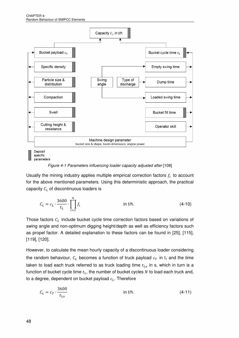
CHAPTER 4: Random Behaviour of SMIPCC Elements
48
Figure 4-1 Parameters influencing loader capacity adjusted after [108]
Usually the mining industry applies multiple empirical correction factors to account
for the above mentioned parameters. Using this deterministic approach, the practical
capacity of discontinuous loaders is
∙ 3600 ∙ in t/h. (4-10)
Those factors include bucket cycle time correction factors based on variations of
swing angle and non-optimum digging height/depth as well as efficiency factors such
as propel factor. A detailed explanation to these factors can be found in [25], [115],
[119], [120].
However, to calculate the mean hourly capacity of a discontinuous loader considering
the random behaviour, becomes a function of truck payload in t, and the time
taken to load each truck referred to as truck loading time in s, which in turn is a
function of bucket cycle time , the number of bucket cycles to load each truck and,
to a degree, dependent on bucket payload . Therefore
∙ 3600 in t/h. (4-11)

4.3 Discontinuous Loader Capacity
49
The quantities , and their random behaviour are discussed further in the following
sections.
Equation (4-11) is not trivial as in general the expected value of quotient of two random
variables is unequal to the quotient of the expected values.
≠ ( )( ) . (4-12)
A mathematical proof is provided in Appendix II.
4.3.1 Bucket Cycle Time
The bucket cycle time consists of the time to swing empty , fill , swing loaded
and dump the bucket. Therefore,
+ + + in s. (4-13)
Bucket cycle time is influenced by the material to be loaded, physical operating
conditions and efficiency of loading equipment operator and machine design
parameters. These influences, with the exception of machine design parameters, tend
to be random in effect and are continuous random variables. Thus is a random
variable.
Bucket cycle time distributions are intuitively positively (right) skewed. Positive
skewness may be explained as minimum values are technically limited in range but
maximum values are less restricted. For example, with a mean bucket cycle time of
30 s a minimum value below 15 s would be unrealistic as the minimum time required
to fill, swing, dump and return is limited to machine design parameters such as rotation
speed, swing angle and boom dimensions. However, maximum values are less
inhibited as in practice time losses, such as attempts of loading equipment operator to
achieve full bucket loads and occurrences of boulders, may add to bucket cycle time.
Distributions of bucket cycle time can typically be modelled by gamma distributions
[90], [114], [121], [122].
A bucket cycle times analysis was conducted at Mittelherbigsdorf basalt quarry for a
Volvo EC460CL hydraulic excavator loading alternately a Volvo A30D articulated dump
truck (28 t payload) and a CAT 771D rigid dump truck (41 t payload). It must be noted
that the excavator was highly “undertrucked”. The term “undertrucked” refers to the
situation when the loading machine is underutilised and trucks will receive their first
bucket load immediately upon entering the loading area because the excavator will be
waiting with its load ready to be dumped onto a truck. Subsequently, the excavator was
able to prepare the muckpile and to fill the bucket before the subsequent truck arrived,
which lead to very large bucket cycle time for the first pass. Therefore, the first bucket
cycle was filtered out and analyses consider only of intermediate bucket cycles
exclusive of the first. Table 4-1 summarizes the sample of bucket cycle times.

CHAPTER 4: Random Behaviour of SMIPCC Elements
50
Table 4-1 Summary of statistical analysis of bucket cycle times
Parameter Intermediate Bucket Cycle Times [s]
# of Records 485
Maximum Value 76
Minimum Value 16
Range 60
Arithmetic Mean 25.06
Standard Deviation 5.59
Coefficient of Variation 0.22
The corresponding histogram is shown in Figure 4-2. For comparison, the gamma
distribution has been fitted with estimates for 33.6 and 1.32. A χ² - test was run
to assess whether the bucket cycle time data can be adequately modelled by a gamma
distribution. The test divides the range of bucket cycle time data into non-overlapping
intervals and compares the number of observations in each class to the number
expected based on the fitted distribution. A χ²-value = 11.88 (with 37 degrees of
freedom) and a P-value = 0.81 were obtained, which means that the hypothesis that
bucket cycle comes from a gamma distribution can be accepted.
Figure 4-2 Histogram of bucket cycle times of Volvo EC460CL
The histogram shows that bucket cycle times can be sufficiently modelled by gamma
distributions with ~ ( , ), shape parameter and scale parameter . Hardy
[114] confirms this observation in his work.
(4-14)
(4-15)

4.3 Discontinuous Loader Capacity
51
The variance of bucket cycle time can be calculated using the following equation
( ∙ ) , (4-16)
where is the coefficient of variation. Typical values of are around 0.1 and 0.3 for
bucket cycle time. Estimates for mean bucket cycle times of different loaders are
provided in [114].
4.3.2 Bucket Payload
The bucket payload , measured in t, is the random mass of digging material held in
the bucket after disengaging from the bank [123] and is expressed as follows:
∙ ∙ ∙ in t (4-17)
where:
is the rated bucket volume in m³ resulting from geometrical bucket dimensions, which
is calculated by agreed standards. The most common standards are (Figure 4-3):
• Struck capacity which refers to the amount of water that the bucket can hold at
maximum when the upper bucket rim is held horizontal,
• Heaped capacity 1:1 (SAE – Society of Automotive Engineers) in which an extra
amount of material with an embankment slope of 1:1 is added to the struck
capacity, and
• Heaped capacity 1:2 (CECE – Committee of European Construction
Equipment) in which an extra amount of material with an embankment slope of
1:2 is added to the struck capacity.
Figure 4-3 Bucket capacity

CHAPTER 4: Random Behaviour of SMIPCC Elements
52
is the in situ density in t/m³ which is an inherent property of the material to be mined.
is the swell factor. It refers change in volume of the mined material which occurs
after disturbance by blasting and loading and can be expressed by the ratio of loose
material density and . In some literature, swell factor is defined as the ratio of insitu
to loose material density, but for the purpose of easy factorisation the reciprocal is used
(4-18)
is the bucket fill factor which depends on muck pile conditions, the bucket geometry,
loader dynamics and material properties [119]. It is defined as the ratio of the actual
volume in the bucket and the rated bucket Volume . The fill factor may be less than
or greater than 1.0. Darling [14] provides a table to estimate fill factors for different
material types.
The actual bucket payload in each pass in the process of loading a mining truck is
influenced by several factors as discussed in the previous subchapter. These factors
are strongly correlated. For instance, muckpile characteristics such as fragmentation
that determines material swell likely influence the operator ability to achieve
consistently high bucket fills and may also constrain digability by affecting penetration
of the face. Additionally, bucket cycle time may also be influenced by the operator
attempt to achieve high bucket fills. In general, factors influencing bucket payload
variability are random, hard to predict and to control [124].
To describe the random behaviour of bucket payloads a literature review was carried
out to obtain the required information.
Schwate [121] investigated in his PhD thesis the bucket payloads of a UB 1212, E302
and EKG 4.6 at a quarry in Germany. He showed that the variation of bucket payload
increases with poor material fragmentation and may be approximated by a beta
distribution with a coefficient of variation between 0.15 and 0.32. However, because of
the lack of an appropriate scaling mechanism the bucket payload was estimated based
on volumetric fill of the bucket, which leaves his results inconclusive.
Hardy [114] conducted a broad bucket payload study in his PhD thesis by analysing
over 350 records from real time observations using Caterpillar’s VIMS/TPMS (Vital
Information Management System / Truck Payload Management System). Results from
this study are summarized in Chanda and Hardy [124]. The interpretation of the results
stated the following:
• Normal distribution can be used to predict the behaviour of all bucket payload
variations.
• Bucket payload of the first pass is comparatively high as operators tend to have
an abundance of time for first pass due to truck manoeuvre and spot time.

4.3 Discontinuous Loader Capacity
53
The results of the statistical analysis of bucket payload for two data sets, one based on
a hydraulic excavator and the other based on a front end loader, are summarized in
Figure 4-2 [114].
Table 4-2 Summary of bucket payload data
Parameter Data set 1 Data set 2
Loading equipment Hydraulic excavator Front-end loader
Truck payload [t] 220 220
Avg. number of bucket cycles 4.44 8.88
Mean bucket payload (all cycles) 50.52 23.93
Mean bucket payload (intermediate cycles)
50.4 23.41
Coefficient of variation – bucket payload (all cycles)
0.275 0.269
Coefficient of variation – bucket payload (intermediate cycles)
0.223 0.187
Figure 4-4 illustrates the summary of bucket payloads of a 700 t hydraulic excavator
with an approximate bucket payload of 50 t loading a 220 t truck in a histogram with an
overlying normal distribution data used from [114].
Figure 4-4 Histogram of bucket payload (all cycles) of the 700t hydraulic excavator
A χ² - test was run to assess whether the bucket payload data can be adequately
modelled by a normal distribution. The test divides the range of bucket payload data
into non-overlapping intervals and compares the number of observations in each class
to the number expected based on the fitted distribution. A χ²-value = 50.77 (with 37
degrees of freedom) and a P-Value = 0.07 were obtained and the hypothesis that
bucket payload data comes from a normal distribution can be accepted.

CHAPTER 4: Random Behaviour of SMIPCC Elements
54
In conclusion, it will be assumed that bucket payload can be approximated by a normal
distribution with ~ ( , ).
The mean bucket payload and its variance can be calculated using the following
equations
∙ ∙ ∙ (4-19)
and
( ∙ ) . (4-20)
Typical values of are around 0.1 and 0.3 for bucket payload.
4.3.3 Truck Payload
Recent literature suggest that the normal distribution fits truck payload data well [122],
[124], [125]. Data provided by Hardy [114] reassures this assumption. However, as
illustrated in Figure 4-5, which shows the histogram of 73 truck payloads of a 220 t
class truck, the histogram is bound to a maximum value. That limit may be understood
as the loader operator’s commitment to follow the 10/10/20 loading policy.
Figure 4-5 Truck payload histogram
The determination of truck payload in t required a more detailed analysis as it
represents the sum of a limited number of bucket payloads. Consequently, the
descriptive statistics of truck payloads are related to all bucket loads in the sub-sample,
which means that in process of loading a truck the underlying variability of individual
bucket payload in conjunction with the number of bucket cycles required to fill the truck
determines the variability of truck payloads.
Therefore, as a prerequisite, it is required to determine the probability of the number of
bucket cycles.

4.3 Discontinuous Loader Capacity
55
In general, the number of bucket cycles varies depending on the maximum acceptable
truck payload and the bucket payload . It must be noted that is a random
variable as elaborated in subchapter 4.3.2. is a fixed parameter, which may be
adjusted by a percentage of the nominal truck payload.
is based on a 10/10/20 payload policy guideline developed by various truck
manufacturers, which states the following: actual payloads between 110% and 120%
of rated payload are allowable but, must not exceed more than 10% of all loads in
a given period, and no single overload greater than 120% of rated payload (maximum
overload factor ) is allowed under any circumstances [126]. The following holds
∙ . (4-21)
A naïve deterministic approximation of the number of bucket cycles required to fill a
truck is given by the ratio of the maximum acceptable truck payload and the mean of
bucket payload.
≈ . (4-22)
In practice, the truck payload is rarely an integer multiple of the bucket payload.
Depending on the loading methodology of the mine, namely full truck or full bucket
strategy, the loader may or may not pass an incomplete bucket to fill the remaining
truck payload amount.
• The full truck strategy means that the loader operator aims to fill the truck even if
the last pass only requires a part of the bucket payload.
• In the full bucket strategy, the aim is to only ever load the truck with full bucket
loads.
The majority of mine operators have the objective to fully utilise the loader. Therefore,
the following is based on the full bucket strategy.
As elaborated in the previous chapter bucket payload is a normally distributed random
variable ~ ( , ) and therefore the number of bucket cycles varies within a
certain spread around the mean value depending on the amount of the individual
bucket payloads.
For the subsequent truck payload and also truck loading time calculations it is
necessary to determine the probability of number of bucket cycles. The following
equations were elaborated during consultations with Dr. Felix Ballani from the Institute
of Stochastics (TU Freiberg) and are based on established equations of probability
theory.
Let be the random number of bucket cycles required to fill a truck. Furthermore, let
, , … be a sequence of independent and identically distributed bucket payloads with

CHAPTER 4: Random Behaviour of SMIPCC Elements
56
the same distribution as , ( ) be the probability that exactly number of
bucket cycles are required to fill the truck and ( ) be the distribution function of the
standard normal distribution.
Set,
( ) (4-23)
for 1,2, … it holds
( ) ( ) ( ) ( ) − ( )
( ) −√
−√
− ( ) − ( + 1)√ + 1
− ( + 1)√ + 1
−√ − − ( + 1)
√ + 1 . (4-24)
For illustration, Figure 4-6 shows the probability distribution of for different
coefficients of variation of using a P&H 4100XPC with a mean bucket payload
102 t to load a Komatsu 960E with a nominal payload capacity of 327 t, which
translates to a maximum truck payload of 359.7 t applying an overload factor of
1.1 to account for the “10” part of the 10/10/20 loading policy [127], [128]. Using the
deterministic equation (4-24) a number of bucket cycles 3.52 is obtained.
Figure 4-6 Number of bucket cycles probability
It can be seen that with increasing variation of bucket payload the variation of the
number of bucket cycles required to fill the truck increases as well.

4.3 Discontinuous Loader Capacity
57
Based on the above it is now possible to describe the distribution function ( ) of the
truck payload. It is clear that . ( ) can be expressed as
Where | ( ) is the distribution function ( ) under the condition that passes
are handled and under the consideration of the truck payload policy.
Using
| ( ) ( ) ( ( ) , ) ( ( ) , ( ) < ( ))
( ( ) , < ( )) (4-26)
It can be seen that
( ) ( ( ) , < ( ))
( ; , ) ( ; , )
( ; , ) 1 − − − . (4-27)
Practically, the sum of only extends over a few (usually between 2 and 7 bucket
cycles). In particular, for a sufficiently large . Therefore, the probability density
function of can be derived as the following holds
( ) ; , 1 − − − . (4-28)
Thus, the mean and variance of can be written as
( ; , ) 1 − − − (4-29)
and
( ) | ( ) , (4-25)

CHAPTER 4: Random Behaviour of SMIPCC Elements
58
( − ) ( ; , 1 − − − . (4-30)
A program developed by the author is used to compare results from the above
equations to actual site data.
Actual site data was provided by Clermont Coal Mine for the primary loading equipment
(P&H 4100) while the truck fleet included Komatsu 830E and 930E. A data analysis of
payload records for the P&H4100 and the Komatsu 930E was carried out and revealed
the following parameters. The sample data can be found in Appendix III.
Table 4-3 Data analysis parameters
Parameter Value from site
data
Values calculated based on equation (4-29) and
(4-30)
Loader parameter
Mean bucket payload [t] 105.26 105.26
Standard deviation of bucket payload [t] 25.57 25.57
Mean bucket cycle time [s] 20.82 20.82
Standard deviation of bucket cycle time [s] 5.09 5.09
Mean number of bucket cycles [#] 2.77 2.70
Standard Deviation number of bucket cycles [#] 0.43 0.48
Truck parameter (Komatsu 930E)
Rated payload [t] 276.8 276.8
Maximal acceptable truck payload [t] 332.2 332.2
Maximum overload factor [-] 1.2 1.2
Mean truck payload [t] 283.94 284.40
Standard deviation of truck payload [t] 25.57 37.32
Number of samples 306
Figure 1-1 shows the distribution of number of bucket cycles of actual site data and the
calculated values.

4.4 Truck Capacity
59
Figure 4-7 Comparison of number of bucket cycles probability
TRUCK CAPACITY
The mean hourly truck capacity is a function of the mean truck payload and truck
cycle time . It holds
∙ 3600 in t/h (4-31)
was discussed in the previous section and truck cycle time is comprised of four
time components
• truck loading time from the truck perspective ,
• travel time ,
• manoeuvre and spot at the loader ,
• manoeuvre and dump at crusher , Therefore
+ + + in s. (4-32)
The individual time components are discussed in turn.
4.4.1 Truck Loading Time
Similar to truck payload, truck loading time is a random variable. Numerous
distribution functions have been applied to describe truck loading times, starting from
• exponential distribution – which is not realistic, as in practice standard deviation
of truck loading times ranges between 0.2 and 0.4 whereas for an exponential
distribution the coefficient of variation is 1, but employed in queueing theoretical
calculations because of its convenient properties [110], [129]–[133];
• through Weibull distribution with two or three parameters [134]–[136];

CHAPTER 4: Random Behaviour of SMIPCC Elements
60
• logarithmic-normal distribution [137];
• Erlang distribution [138] and
• normal distribution [96], [124], [125], [139]–[141].
• Finally, Stoyan [142] and Wang et al. [143] suggested to model truck loading
time using an inverse Gaussian distribution.
Before discussing the appropriate distribution of truck loading time it is necessary to
review practical loading methods and the loading procedure itself, as this can have a
significant impact on productivity [144].
Generally, four primary loading methods exist (refer to Figure 4-8 and Figure 4-9):
• single-side method,
• double-side method,
• drive-by method and
• modified drive-by method.
Figure 4-8 Single-side method (left) and double-side method (right)
Figure 4-9 Drive-by method (left) and modified drive-by method (right)
Although promising efficiency improvements by double-side and drive-by loading
methods can occur, the current standard loading method in Australian coal mines and
others is single-side loading [145] with the trucks to the left when addressing the face
and is therefore a basis for further discussions.

4.4 Truck Capacity
61
Two additional cases can be considered, which are shown in Figure 4-10 and Figure
4-11.
• Case a represents a scenario in which trucks queue in front of the loading zone
ready to manoeuvre and spot into loading position.
• Case b represents a scenario in which the loader is waiting for trucks and a soon
as the loader operator notices a truck approach the bucket cycle pass is initiated.
In both cases the loader will pause for a residual time until the spot position is reached
and the shovel dumps. This time is referred to as loader inherent wait time and is
the difference between manoeuvre and spot time of the truck at loader and the time
required for the first bucket cycle.
− (4-33)
Typical inherent wait time for loading equipment to be ready ranges between 10 and
15 seconds depending on the truck and loading equipment.
This time can be seen as inherent operating delay however it is inevitable in a single
side loading operation and is therefore added to truck loading time.
Figure 4-10 Truck loading scenario - Case a
Figure 4-11 Truck loading scenario - Case b
Considering the above, truck loading time can be viewed from two perspectives. Firstly,
from the loading equipment and secondly from a truck perspective.

CHAPTER 4: Random Behaviour of SMIPCC Elements
62
• Truck loading time from the loading equipment perspective represents an
accumulation of a limited number of bucket cycle times and inherent loader waiting
time.
• Truck loading time from the truck perspective represents an accumulation of
the dump time of the first bucket cycle immediately on spot – generally between
3 and 5 s depending on material properties, bucket load and release mechanism
[114] – and the second through to the final bucket cycle to fill the truck according
to payload policies.
This statement translates into the following deterministic equations
+ in s. (4-34)
+ in s. (4-35)
According to the central limit theorem [112], the distribution of the sum of independent
random variables tends to be normally distributed regardless of the distribution of the
summed components. As shown in equation (4-34) truck loading time is equal to a
certain number of bucket cycle times. Each bucket cycle time is a random variable (see
sub-chapter 4.3.1) and the individual cycle times may be considered as independent
of each other. It could therefore be expected that truck loading times are normally
distributed [96], [124], [125], [139]–[141].
However, as elaborated in the previous section, truck loading time depends
significantly on the number of bucket cycles required to fill the truck which in turn is
dependent on the bucket payload for each pass. Therefore, the true distribution of truck
loading time is a superposition (bimodal distribution) of a number of normal
distributions, each having a specific mean and variance. Which means that multiple
peaks for loading time are possible. A histogram (Figure 4-12) provided by Czaplicki
[96] clearly shows this effect described above. In this example the mean bucket cycle
time may be approx. 26 s, which translates into a total of 4 and 5 bucket cycles for the
normal distributions indicated in blue and red, respectively.

4.4 Truck Capacity
63
Figure 4-12 Histogram of truck loading time with two superposed normal distribution
Calculation for blue normal distribution
+ 12 + 26 ≈ 1.9 (4-36)
Calculation for red normal distribution
+ 12 + 26 ≈ 2.3 (4-37)
Similar to the calculation for the described relationship for truck loading time can by
determined as follows. Let be gamma distributed with ~ ( , ) as shown in
sub-chapter 4.3.1, where / is the shape parameter and / the scale
parameter, due to the convolution stability of the gamma distribution ( )~ ( , ) [146]. Under the assumption that and are stochastically
independent the sequence of bucket cycle times is independent of the number of
bucket cycle times . The probability density functions ( ) and ( ), are then
( ) ( ; / , / ) ∙ (4-38)
−√ − − ( + 1)
√ + 1
and
( ) + ( ; / , / ) ∙ (4-39)

CHAPTER 4: Random Behaviour of SMIPCC Elements
64
−√ − − ( + 1)
√ + 1 .
Independent of all distributional assumptions the mean truck loading times and
are given by
in s (4-40)
and
( −1) + in s. (4-41)
Its variances are equal to
+ ( ) in s² (4-42)
and
( − 1) + ( ) in s². (4-43)
4.4.2 Travel Time
Truck travel time is an important figure for capacity calculations. The truck times on
a haul road depend on the truck engine characteristics, the haul road profile and its
conditions, the payload on the truck, and to a degree, even on the number of trucks (e.
g. truck bunching [125]). Truck bunching or clumping refers to the process of faster
trucks being delayed behind slower trucks. where overtaking is prohibited due to haul
road restrictions. This is a source of considerable productivity loss for truck haulage
systems in large open pits. The main influence on truck travel time is the truck payload.
Travel time is therefore divided into truck travel time unloaded and truck travel
time loaded . It holds
+ in s. (4-44)
To further account for the effect of haul road grade and conditions, haul roads are
generally divided into segments corresponding to changes in gradient or surface
conditions. The estimates for each segment are then added to provide an estimate of
the total travel time.
Data provided by Panagiotou [133] also suggest that truck travel times are well fitted
by an inverse Gaussian distribution (refer to Figure 4-13). A χ² - test with a sample size
of 93 reveals a P-value of 0.373 for an inverse Gaussian distribution compared to 0.138
for a normal distribution.

4.4 Truck Capacity
65
Figure 4-13 Travel time distribution - data used from [133]
According to relevant literature truck travel times may be successfully described by a
normal distribution [90], [96], [139], [143], [147], [148]. Data obtained by the author
reaffirm this assumption. Figure 4-14 shows histograms of travel times from loaded
(left) and unloaded (right) trucks with overlaid IGD (inverse Gaussian distribution) and
normal distribution. The data was obtained by the author during a time study at the
basalt quarry Mittelherbigsdorf. The total sample size corresponds to 35
measurements. A χ² - test indicated a p-value of 0.49 for loaded travel times and further
0.67 for unloaded truck travel time for a normal distribution. For comparison, the
inverse Gaussian distribution is indicated in blue. Both distributions fit the samples
quite well.
Figure 4-14 Travel time distribution loaded (left) unloaded (right)
Both distributions deliver sufficient results, depending on the purpose of the
investigation. However, for pragmatic reasons, the normal distribution sufficiently
represents truck travel times, which is therefore applied in this thesis.
The variance of can be predicted using estimates of coefficient of variation . Hardy
[114] states a of 0.12 to 0.53 in his PhD thesis. Barnes et al. [110] suggested a
coefficient of variation between 0.1 and 0.2. A comprehensive truck travel time study
under different operation conditions undertaken by Caterpillar [149] reaffirmed the
suggested coefficient of variation from Barnes. Contradicting conclusions are made by
Barnes and Stoyan [147] with regards to behaviour of variance of truck travel times
and section lengths. Barnes states that variance of travel time decreases with
increases in overall segment length whereas Stoyan states the opposite. However,

CHAPTER 4: Random Behaviour of SMIPCC Elements
66
Stoyan’s statement is purely based on the behaviour of the inverse Gaussian
distribution in which the variance increases with higher mean values. The author
agrees with the statements made by Barnes and Hardy that the variance of truck travel
times decreases with section length, due to the fact that the truck operator has a certain
control over the velocity within the mines speed regulations and will therefore attempt
to regain lost time of one segment in the other.
The variance of truck travel time can be calculated using the following equation
( ∙ ) . in s². (4-45)
4.4.3 Manoeuvre and Spot Time at Loader
Manoeuvre and spot time at the loader consist of the time to turn, reverse and spot
the truck to get loaded. It depends on the physical parameters of the truck,
manoeuvring safety practice and available bench space. As these times are relatively
short the variation can be neglected and it is sufficient to use mean values. Mean times
for truck spot times at the loader are suggested:
• “Usually between 0.4 to 0.7 minutes” [150]
• “Typically between 0.6 to 0.8 minutes” [151]
• “0.75 minutes for 220 tonne trucks is a typical value” [114]
4.4.4 Manoeuvre and Dump Time at Crusher Station
Manoeuvre and dump time consists of raising the body, the time required for the
material to flow out of the body, lowering the body and the manoeuvre time. Combined
are generally 60 s for rear dump trucks and 30 s bottom dump trucks [150].
Caterpillar [151] provides a typical range for of 60 - 80 s for rear dump trucks. The
author’s experience is that of 45 s for quarry trucks and 60 s for large mining trucks
is a reasonable (and typical) value. Nevertheless, experience made by the author in oil
sand operations (Aurora mine, Canada) showed that unloading time may be up to 75 s.
The unusual high unloading time results from the sticky material behaviour.
Similar to manoeuvre and spot time at the loader are manoeuvre and dump times; they
are comparatively short and thus mean values are sufficient for approximations.
Additionally studies made by Wang et al. [143] suggest that manoeuvre and dump
times are relatively stable and conclude that they can be regarded as constant.
DISTURBANCE BEHAVIOUR OF SYSTEM ELEMENTS
The disturbance behaviour of individual elements has an essential impact on the
behaviour of the entire system. Therefore, the disturbance behaviour of individual
SMIPCC system elements will now be explained in detail. It can be described by the
period of time of a respective disturbance and the operational time between two

4.5 Disturbance Behaviour of System Elements
67
subsequent disturbances. Those periods of times are, as it is clear, random variables
and can be statistically analysed.
Since at this point only the individual elements are of interest, disturbances caused by
other system elements are excluded from the following discussion. Furthermore,
planned downtimes are omitted.
Schematically the system process can be illustrated as shown in Figure 4-15. Gladysz
[152] called the corresponding stochastic process general operation process. The
general operation process needs to be investigated when questions related to
disturbance and repair behaviour of system elements are discussed.
Figure 4-15 Schematic illustration of general operation process of system elements
However, in case of system capacity and time usage calculations the general operation
process is far too complicated. It is therefore simplified by combining certain states.
Gladysz suggested the first reduction step in which the process is simplified by only
distinguishing between operational state and disturbance state. The resulting
stochastic process is called simplified operation process and is illustrated in Figure
4-16.
Figure 4-16 Schematic illustration of simplified operation process of system elements
The simplified operation process formally complies with a serial connection of abstract
elements , … , (e.g. motor, belt, alignment switch), which constantly alternate
between “operation” and “disturbance”. This implies that when the simplified operation
process is in operational state, all elements , … , are operational.

CHAPTER 4: Random Behaviour of SMIPCC Elements
68
Gladysz suggested the second reduction step to further simplify the process. In the
second reduction step the disturbance cause is dismissed and the process is reduced
to operational state and disturbance state. The resulting stochastic process is called
elementary operation process and is illustrated in Figure 4-17.
Figure 4-17 Schematic illustration of elementary operation process of system elements
4.5.1 Characteristics of Elemental Operational Process
The disturbance behaviour of system elements is characterised by the following three
quantities:
1. distribution function of repair time
2. distribution function of work time,
3. repair ratio.
The term repair time is used to denote the period of time in which the element stands
still due to inherent breakdown. Inherent breakdowns are e.g. due to operational,
geological, mechanical, electrical and control failures. The failure time commonly
comprises of waiting time for repair, repair time itself and preparation time to set the
element back into operation.
The work time, also referred to as time to failure, is defined as the period of time
between two inherent breakdowns of the considered element. This period of time may
be interrupted due to planned maintenance or breakdowns of connected elements.
Figure 4-18 illustrates schematically the time between two subsequent disturbance
periods.
Figure 4-18 Schematic illustration of work time of a system element

4.5 Disturbance Behaviour of System Elements
69
The repair ratio is a quantity derived from the distributions of repair time and work
times. It is simply the ratio of the mean values of repair time and work times.
In literature many distributions have been used to represent the disturbance behaviour
of system elements. Generally, stationary distributions are used. For those, the
probability distribution at any time , , … must be the same as the probability
distribution at times + , + , … + , where is an arbitrary shift along the time
axis [153]. In the context of maintenance, the assumption of a stationary process
implies that the distribution of failures after any repair is the same after every repair.
This also implies that the element is in the same condition after the repair as it was
when new. In reality this is not true because of [154]
• replacement parts are not identical,
• variation in maintenance practice, and
• equipment life itself.
However, it is a necessary simplifying assumption.
To facilitate the research, data and information from computerized maintenance
management systems of 11 different mining operations in five countries including
Australia, Canada, Chile, China and Germany was obtained. Commodities included
sub-bituminous coal and lignite, oil sand, copper and iron ore. Table 4-4 summarises
the collected data.
Table 4-4 Summary of data collection
Mining Operation
Country Commodity Observation
period
SMIPCC system element
Discontinuous system
Continuous system
Loader Truck Crusher Conveyor Spreader
1 Australia Coal 4 years x x x x x
2 Canada Copper 1 years x x x - -
3 Canada Oil Sand 2 years x - x - -
4 Chile Copper 3 years - - x - -
5 China Coal 1 year - - - x x
6 China Coal 1 year - - x x x
7 China Iron 1 year - - - x x
8 China Copper 2 years - - x x x
9 Germany Lignite 4 years - - - x x
10 Germany Lignite 4 years - - - x x
11 Germany Lignite 2 years - - - x x
x data obtained - no data obtained
The raw maintenance time data was reviewed and three levels of filters were
successively applied, including:

CHAPTER 4: Random Behaviour of SMIPCC Elements
70
1. filter level 1 – filtering of obviously non-comparable, erroneous or anomalous
records,
2. filter level 2 – filtering of planned downtimes ,
3. filter level 3 – categorising unplanned downtimes according to the time
usage model described in chapter 5.1 whenever possible.
4.5.2 Repair Time
The repair time can be modelled as a random variable. Its actual duration is not readily
predictable. If a system element is operating under similar conditions for a longer period
of time it can be expected that the occurrence of individual repair time follows a certain
distribution. It is thus presumed that for the repair times of elements fixed probability
distributions exist, which of course depend on mining conditions, element types and
quality of maintenance management.
The distributions of system element repair times have been analysed for many years,
and many publications report on them. They include lognormal, gamma, exponential
and Weibull distributions. Table 4-5 provides a summary of literature on repair times
and their distributions of relevant SMIPCC system elements.
For the majority of distributions provided in Table 4-5 it remains unclear what raw data
were taken into consideration. For example Temeng [155] divided repair data of trucks
into electrical and mechanical types of repairs. He found that histograms electrical
repair times were accurately described by an exponential distribution while for
mechanical repair times gamma or Weibull distributions delivered better results.
Histograms of mechanical repair times and compound clearing times were frequently
positively asymmetrical. Furthermore, mean repair times for loaders and trucks
provided by Shama et al., Elevili et al. and Hall [156]–[158] are comparatively high. The
reason might be that small disturbances have not been considered.

4.5 Disturbance Behaviour of System Elements
71
Table 4-5 Literature on repair time and associated distribution
Source Element Material Mean Repair
Time [min]
Best-Fit
Distribution
[159] Spreader Coal 32.4 Lognormal
Conveyor Coal 10.2-29.4 Lognormal
[156] Truck Copper 230-321 Lognormal
[160] Crusher
(Gyratory) Bauxite n.a. Lognormal
Conveyor 1.42 Lognormal
[157] Loader Coal 236-588 Lognormal
[161] Trucks n.a. 480 Lognormal
[93] Spreader Coal 78 Exponential
Conveyor Coal 84-90 Exponential
[105] Loader
Coal n.a. Weibull 3P
Truck n.a. Weibull 3P
Crusher n.a. Weibull 3P
[147] Spreader Lignite 15-60 Exponential
Conveyor Lignite 15-60 Exponential
[155] Loader Copper n.a. Gamma / Weibull
[162]
Conveyor (mobile)
n.a. 24-48 Exponential
Conveyor (fixed)
n.a. 42-72 Exponential
Spreader n.a. 90 Exponential
[163] Crusher n.a. 120 Weibull
Conveyor n.a. 114 Weibull
Spreader n.a. 162 Weibull
[158] Truck n.a. 317-355 Lognormal
In this thesis, the data analysis undertaken considered all disturbances (unplanned
downtimes) except crusher and loader idle time (wait for trucks). Unplanned downtime
causes common for all system elements include:
• electrical breakdowns,
• mechanical breakdowns,
• equipment protection trips,
• accidental damage.
Additional, element specific unplanned downtime causes are shown in Figure 4-19.

CHAPTER 4: Random Behaviour of SMIPCC Elements
72
Figure 4-19 Element specific unplanned downtime causes
The results showed that the exponential distribution describes the empirical data of
relevant equipment repair times well. As an example, Figure 4-20 shows the histogram
of repair time data of a crusher station working in a coal mine for overburden removal
and gives cause to an interesting discussion.
At first sight it seems that the data of repair times cannot be well fitted by an exponential
distribution. Very small disturbances have a much higher frequency than expected for
the fitted exponential distribution. In contrast, many authors work with distributions such
as lognormal, gamma or Weibull (see Table 4-5), in which small disturbances are
almost excluded.
The discrepancy may presumably be explained by different methods of data collection.
While the author mainly used data recorded by automatic data collection systems, in
which even the smallest disturbances were recorded, disturbance data from older
literature was commonly recorded by an operator. In the latter case the data collection
is highly influenced by subjective effects, which in turn may lead to results where small
disturbances are either not recorded or rounded up to the next full minute.
For realistic and simple modelling, the exponential distribution appears most
reasonable, as many very small disturbances have no influence on the operation. Thus,
the part of repair times which has a high frequency between 0 and 1 minutes, should
not be taken into consideration.
Selected site data for individual SMIPCC system elements repair time is provided in
Appendix IV.

4.5 Disturbance Behaviour of System Elements
73
Figure 4-20 Repair time histogram of a crusher station
When recalling equation (4-7) the distribution function of the exponential distribution is
given by
( < ) 1 − , 0, (4-46)
where denotes the repair time. Equation (4-46) means that the probability that a
repair with a duration smaller than occurs equals 1 − .
The mean repair time equals
1 in min. (4-47)
Thus, if the repair time is exponentially distributed the information on the mean repair
time is sufficient to fully characterise the distribution. Mean repair time is possibly the
most common measure or parameter in maintainability analysis and is utilised to
determine corrective maintenance times.
The mean repair time can be interpreted as a measure of the maintenance organisation
[147]. For small mean repair time the average times to repair a piece of equipment is
short – repairs happen quickly. For large mean repair time certain deficiencies of the
maintenance organisation are present (e.g. missing spare parts, insufficient
personnel). Nonetheless, individual operational conditions of system elements are
quite variable, so that large mean repair time may not necessarily indicate a bad
maintenance organisation.
Statistically is determined by the sample mean of repair times.
A summary of mean repair time based on the data collected by the author as described
in Table 4-4 is indicated in Table 4-6.

CHAPTER 4: Random Behaviour of SMIPCC Elements
74
Table 4-6 Summary of mean repair time of SMIPCC system elements
Equipment type Sample
size
Mean Repair Time [min]
Min Mean Max CV
Loader
cable shovel 11 64.0 132.7 233.5 0.35
hydraulic excavator 13 134.2 288.1 626.5 0.54
Trucks 20 114.5 296.7 676.3 0.67
Crusher 10 14.7 33.1 55.9 0.46
Spreader 19 33.6 52.1 88.9 0.40
Conveyor
shiftable 29 10.0 32.7 67.3 0.51
relocatable 21 10.1 31.8 60.8 0.45
fix 26 9.8 21.0 32.5 0.35
4.5.3 Work Time
The period between two consecutive disturbances/repairs is called work time. Work
times is, just as repair time, a random variable. It also applies that under similar
operating conditions a certain distributions functions for work times of system elements
can be obtained. Publications which consider work times of system elements in mines
are listed in Table 4-7.
Table 4-7 Literature on work times and associated distributions
Source Element Material Mean Work Time
[min]
Best-Fit
Distribution
[159] Spreader Coal 8,950 Weibull
Conveyor Coal 1,559 -3,155 Lognormal
[160] Crusher
(Gyratory) Bauxite n.a. Weibull
Conveyor 15.25 Lognormal
[161] Trucks - 120 Exponential
[93] Spreader Coal 900 Exponential
Conveyor Coal 1,710-2,040 Exponential
[105] Loader Coal n.a. Weibull
Truck Coal n.a. Gamma
[158] Truck - 688-869 Lognormal
The statistical analysis of work times of system elements in much more difficult than
for repair time because interruptions of work time occur because of planned downtimes
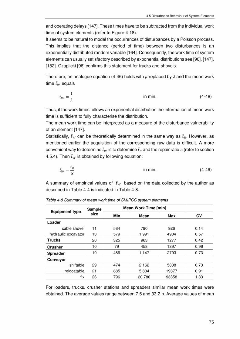
4.5 Disturbance Behaviour of System Elements
75
and operating delays [147]. These times have to be subtracted from the individual work
time of system elements (refer to Figure 4-18).
It seems to be natural to model the occurrences of disturbances by a Poisson process.
This implies that the distance (period of time) between two disturbances is an
exponentially distributed random variable [164]. Consequently, the work time of system
elements can usually satisfactory described by exponential distributions see [90], [147],
[152]. Czaplicki [96] confirms this statement for trucks and shovels.
Therefore, an analogue equation (4-46) holds with replaced by and the mean work
time equals
1 in min. (4-48)
Thus, if the work times follows an exponential distribution the information of mean work
time is sufficient to fully characterise the distribution.
The mean work time can be interpreted as a measure of the disturbance vulnerability
of an element [147].
Statistically, can be theoretically determined in the same way as . However, as
mentioned earlier the acquisition of the corresponding raw data is difficult. A more
convenient way to determine is to determine and the repair ratio ϰ (refer to section
4.5.4). Then is obtained by following equation:
in min. (4-49)
A summary of empirical values of based on the data collected by the author as
described in Table 4-4 is indicated in Table 4-8.
Table 4-8 Summary of mean work time of SMIPCC system elements
Equipment type Sample
size
Mean Work Time [min]
Min Mean Max CV
Loader
cable shovel 11 584 790 926 0.14
hydraulic excavator 13 579 1,991 4904 0.57
Trucks 20 325 963 1277 0.42
Crusher 10 79 458 1397 0.96
Spreader 19 486 1,147 2703 0.73
Conveyor
shiftable 29 474 2,162 5838 0.73
relocatable 21 885 5,834 19377 0.91
fix 26 796 20,780 93358 1.33
For loaders, trucks, crusher stations and spreaders similar mean work times were
obtained. The average values range between 7.5 and 33.2 h. Average values of mean

CHAPTER 4: Random Behaviour of SMIPCC Elements
76
work time for conveyors are considerably higher and range from 36 to 346 h,
respectively.
Obviously, has the amount and quality of preventative maintenance a substantial
influence on the mean work time which may explains the relatively high coefficient of
correlation of the provided data in Table 4-8.
4.5.4 Repair Ratio
The repair ratio ϰ of a system element is defined as
. (4-50)
The quantity ϰ is a non-dimensional parameter. It is a measure of the frequency of
disturbances of a system element and is important for further calculations. For large ϰ,
the time in which an element is disturbed is large. The quantity ϰ can be decreased by
increasing (by enhanced preventative maintenance or constructive improvements)
or/and by decreasing (enhance maintenance organisation). Statistically ϰ is
determined as follows. The operation time ( ) and the unplanned downtime ( )
of an element in the observation period (e.g. one or several months) are determined.
Then ϰ is estimated by
( ) ( ) . (4-51)
Table 4-9 lists ϰ values which were statistically derived during the course of this thesis
for relevant equipment. These values compare very well with those provided by other
authors [90], [147], [165]. That the more recent values are smaller than the older ones
can be explained by technological progress, such as increased component reliability
and enhanced condition monitoring, over the last decades.
Table 4-9 Summary of repair ratio values of SMIPCC system elements
Equipment type Sample
size
Repair Ratio
Min Mean Max CV
Loader
cable shovel 11 0.083 0.170 0.270 0.35
hydraulic excavator 13 0.091 0.157 0.299 0.40
Trucks 20 0.0310 0.1280 0.2300 0.50
Crusher 10 0.035 0.117 0.238 0.62
Spreader 19 0.022 0.059 0.118 0.48
Conveyor
shiftable 29 0.004 0.019 0.043 0.77
relocatable 21 0.001 0.012 0.050 1.06
fix 26 0.000 0.007 0.035 1.41

77
SMIPCC CAPACITY DETERMINATION
METHOD
Based on the random behaviour of system elements a method is developed to determine the annual capacity of a SMIPCC system. In this chapter a detailed structure is provided to determine the effective operating hours of the system.

CHAPTER 5: SMIPCC Capacity Determination Method
78
GENERAL SMIPCC SYSTEM CAPACITY DETERMINATION
SMIPCC systems are complex material handling systems including various elements
with the function to excavate, haul and discharge material from the operation face in
the mine to a designated destination. As such, variations in capacity of one element
can affects the capacity of other elements of the system.
The SMIPCC system can be defined as an L/T-C/B/D system where L/T stands for the
discontinuous part of the system and C/B/D for the continuous part. Where L is the
number of loader, T is the number of trucks, C is the number of crusher stations, B is
the number of belt conveyors, and D is the number of spreaders. The most simplistic
but also most common system is shown schematically in Figure 5-1.
Figure 5-1 Schematic illustration of simplified SMIPCC system
The capacity of such SMIPCC system for longer time periods is influenced by process
and element specific characteristics as well as by the overall system layout. The
operation of a SMIPCC systems is characterized by a high level of mechanization and
automation as the majority of the transport distance is realized by conveyors. This
creates the requirement for high utilisation of the machine system. The logical
consequence is that capacity planning is carried out in relation to the machine system.
Whereby the winning element (loader) acts as the capacity determining element under
consideration of their technological connections. Once the average hourly capacity of
the winning element is known, the capacity of the entire SMIPCC system can be
determined based on the effective operating time of winning element in h. It holds
in t/a. (5-1)
The determination of the average hourly capacity of the loader is demonstrated in detail in section 4.3. The following section describes a method to

5.2 Time Usage Model
79
determine the effective operating hours of the system under consideration of the
system aspect.
TIME USAGE MODEL
The prerequisite for the calculation of and to commence selection of equipment of
suitable capacity is to investigate the different operational and downtime states of
system elements. This is achievable by a time usage model, which is also referred to
as time allocation model or calendar time structure.
Developing a defined time usage model is an imperative management initiative to
enable determination of time components relevant to productivity determination. It
forms a common basis for benchmarking of mining equipment by providing
standardized definitions and methodologies for measuring reliability, availability and
utilisation performance of equipment in a mining environment. It is also a critical input
to establish required equipment performance and a realistic estimation, in particular for
a “greenfields” project, or determination from historical data, in-house or industry-wide,
of the number of productive hours per year, that can be adopted as a robust basis for
required productivity determinations.
Despite current efforts made by the Global Mining Standards and Guidelines Group
[166], [167] the mining industry has not yet developed a common standard of deriving
or stating equipment performance [168], [169]. Most large mining companies have their
internal “standard” nomenclature and time usage model. Figure 5-2 to Figure 5-4 show
current examples of time usage models from three major mining companies.
Figure 5-2 Open cut time model Xstrata [170]

CHAPTER 5: SMIPCC Capacity Determination Method
80
Figure 5-3 Time allocation model Rio Tinto [171]
Figure 5-4 Time usage model used by Western Premier Coal Limited [114]
Time usage models are of course similar in structure, definitions and equations for
availability and utilisation parameters. For example, calendar time is usually divided
into utilised time, available time and downtime, and further broken down into
subcategories. However, differences in definition behind equations and classification
of occurring operational and downtime state of equipment during the course of a mining
operation create inconsistencies in measuring and reporting.
In order to better analyse the time components of SMIPCC systems the time usage
model shown in the previous section needs to be substantiated in accordance to TGL
32 - 778/01-15 [172]. The TGL is the GDR (German Democratic Republic) equivalent
to the German Industry Standard (DIN). In the author´s opinion this standard
represents the best foundation for material handling systems with combined material
transport. However, as the TGL 32 - 778/01-15 was developed for material handling
systems with continuous transport, several time quantities and their relation to each
other were required to be adjusted.
A specific time usage model for SMIPCC systems (refer to Figure 5-5) is developed in
order to apply a calculation model for the prediction of SMIPCC system capacities. The
following time quantities refer to average values of the generally randomly fluctuating
quantity.

5.2 Time Usage Model
81
Figure 5-5 SMIPCC time usage model
The time usage model divides calendar time (8,760 h per year – ignoring leap years
of 8,784 h per year), primarily into operating time and downtime .
Operating time refers to the period in which the equipment is functioning which
means the service meter unit is running (motor is running). In a certain portion of
operating time the equipment is operating in an unproductive manner. This time refers
to operating delay . The time in which the element is considered to be operating at
full effectiveness is referred to as effective operating time . Hence,
+ in h. (5-2)
Operating delay is divided into self-induced operating delays ( ) and system-induced
operating delays . Self-induced operating delays include periods in which the
equipment is performing its normal operating function, but is hampered by minor short-
term delays such as minor pad preparations, face clean-ups, tramming etc. System-
induced operating delays refer to times the system element is not able to operate due
to the fact that another element is not available, which makes it impossible for the
element to operate effectively. Typically, this time is also referred to as idle time. It
holds

CHAPTER 5: SMIPCC Capacity Determination Method
82
( ) + ( ) in h. (5-3)
Downtimes are initially divided into Planned downtime and Unplanned downtime
.
Unplanned downtime refers to the time the element is unavailable due to
unscheduled maintenance in the form of disturbances or breakdowns.
Planned downtime includes time events that can be scheduled or approximated in
advance. They are further subdivided according to their cause into the following:
( ) – Non-scheduled production
( ) – External disturbances
( ) – Preventative maintenance ( ) – Planned shift delays ( ) – Technological downtime
Then:
( ) + ( ) + ( ) + ( ) + ( ) in h. (5-4)
Non-scheduled production ( )
includes the period of time in which the equipment is
technically available but not scheduled to operate due to factors such as:
• Non-worked holidays,
• Training on equipment,
• No production due to regulations (environmental, governmental).
External disturbances ( )
includes the period of time in which the equipment is
technically available but not utilised due to external factors such as:
• Bad weather (e.g. heavy snow or rain fall, lightning, wind etc.),
• Workforce disputes,
• Power outages.
Although occurrence and duration of external downtimes are in principle not predictable
and should therefore, following the definition be categorized into unplanned
downtimes, regional differences create a strong variation among those downtimes. For
example, a coal mine in Inner Mongolia experiences up to 3 months of downtime due
to harsh winter conditions whereas an Iron ore mine in the Pilbara only experiences 3
to 5 day downtimes due to bad weather, mostly heavy rainfalls [173], [174]. Similar
variations among regions apply to workforce disputes and power outages.

5.3 Calculation of Effective Operating Time
83
Consequently, external disturbances would heavily distort results for unplanned
downtime for individual elements (see sub-chapter 4.5). In addition, downtimes due to
external factors are difficult to assign to a specific element as they usually effect the
entire system.
Preventative maintenance ( )
includes the period of time in which the equipment is
not scheduled to operate in order to carry out preventative maintenance measures or
preparation for such measures. Maintenance practices vary greatly throughout the
mining industry and do not appear to be correlated with the operation size or mining
method. Many mining companies follow manufacturer´s recommendations, while
others developed their own specific maintenance strategy. Recent Literature that is
dealing with this topic includes [175]–[177].
Planned shift delays ( ) are proportional to operating time and refer to periods that
occur as regular shift events. These regular shift events included delays such as travel
time to and from the pit, shift change, meal breaks, equipment inspections and safety
meetings.
Technological downtimes ( ), also referred to as process related downtime, occur
regularly and include time in which the equipment is not operating due to required mine
development or technological changes of the system. This includes
• relocations of crusher stations or conveyors,
• trackshifting of conveyors,
• conveyor belt extensions or shortening
• blasting.
In accordance to the respective IPCC system some of the mentioned time components
may not occur. Those need then to be set to zero. It holds
+ + + in h (5-5)
Equation (5-5) can be used to determine the period of times of interest – primarily .
CALCULATION OF EFFECTIVE OPERATING TIME
For the calculation of the effective operating time each time component described
in section 5.1 needs to be determined. The majority of the time components can be
easily approximated as constants. This includes the time components ( ), ( ), ( ) and
( ) .
Non-scheduled production ( )

CHAPTER 5: SMIPCC Capacity Determination Method
84
Non-scheduled production time is basically the sum of all time components the entire
production process is not scheduled to operate.
External disturbances ( )
External disturbances are basically the sum of all time components when the
production process or a system element is scheduled to operate but is unable to
operate as a result of bad weather (heavy rainfall, lightning, bad visibility due to fog or
heavy winds), labour disputes and environmental regulations.
Preventative maintenance ( )
Similar to the time components described above preventative maintenance is basically
the sum of all times in which an element is not scheduled to operate due to:
• Scheduled maintenance as agreed in the confirmed maintenance schedule;
• Inspections and testing for preventive maintenance, instrument calibration &
safety regulations – but excluding operator pre-start inspections,
• Capital work for modifications and expansions.
In case of the continuous part of the machine system (crusher station, conveyors, and
spreader) maintenance is commonly realised periodically such as weekly, monthly, and
annually [178]. This implies that whenever an element of the continuous part of the
machine system requires preventative maintenance according to agreed intervals or
predictive techniques, the entire system chain is not operating. It is therefore the
maintenance manager’s objective to schedule required preventative maintenance of
continuous system elements as well-timed as possible to maximize operating time
[179]. Thus, to approximate downtime due to preventative maintenance ( ) the
maximum of required maintenance time of each continuous element ( ) in each
maintenance period needs to be considered. However, it also depends on whether
sufficient maintenance resources are available for concurrent maintenance. Typically,
a certain amount of preventative maintenance is outsourced to specialized companies.
Considering the above mentioned the total preventative maintenance time component
can be expressed as follows
( ) ( ) in h (5-6)
Here represents the elements crusher station, conveyors, spreader and
the maintenance periods weekly, monthly, annual maintenance periods.
In the special case which is considered in this thesis, of one loader feeding the

5.3 Calculation of Effective Operating Time
85
continuous part of the machine system, planned maintenance required for the loader
is also included in this equation.
Planned shift delays ( )
Planned shift delays represent the sum of individual planned shift delays ( ) in h/shift
multiplied by the available shifts per annum. To approximate the annual planned shift
delays the following holds
( ) − ( ) − ( ) − ( ) − ( ) ( ) in h (5-7)
Technological downtime proportional to effective operating time ( )
The majority of technological downtimes are proportional to . This includes but is
not limited to times for blasting and conveyor trackshifts. It holds
( ) in h. (5-8)
The factor is referred to technological downtime ratio and is dimensionless.
Technological downtimes proportional to operating time include downtimes due to
conveyor trackshifts and blasting occurrences. They are also based on a certain
volume1. In the case of conveyor trackshifts, the volume represents the maximum
dump block volume . The dump block volume can be calculated depending on the
shifting pattern. In the case of blasting delays, the volume represents the amount of
material for each blast which is referred to as blast volume . That means, as soon
as the maximum dump block volume is exhausted the dump conveyor is required to be
trackshifted. Similar to that, a blasting delay is initiated as soon as the loader depletes
the blast volume (excavatable muckpile material).
The effective operating time ( ) and ( ) required to reach the maximum dump block
volume or blast volume can be approximated by
( ) in h. (5-9)
( ) in h. (5-10)
If the time required for each conveyor trackshifting and each blasting is known,
it is possible to determine by using the following relation
1 Volume is in this thesis translated to tonnage based on a certain density
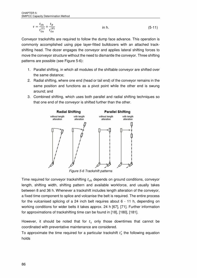
CHAPTER 5: SMIPCC Capacity Determination Method
86
( ) +
( ) in h. (5-11)
Conveyor trackshifts are required to follow the dump face advance. This operation is
commonly accomplished using pipe layer-fitted bulldozers with an attached track-
shifting head. The dozer engages the conveyor and applies lateral shifting forces to
move the conveyor structure without the need to dismantle the conveyor. Three shifting
patterns are possible (see Figure 5-6):
1. Parallel shifting, in which all modules of the shiftable conveyor are shifted over
the same distance;
2. Radial shifting, where one end (head or tail end) of the conveyor remains in the
same position and functions as a pivot point while the other end is swung
around; and
3. Combined shifting, which uses both parallel and radial shifting techniques so
that one end of the conveyor is shifted further than the other.
Figure 5-6 Trackshift patterns
Time required for conveyor trackshifting depends on ground conditions, conveyor
length, shifting width, shifting pattern and available workforce, and usually takes
between 8 and 36 h. Whenever a trackshift includes length alteration of the conveyor,
a fixed time component to splice and volcanise the belt is required. The entire process
for the vulcanised splicing of a 24 inch belt requires about 6 - 11 h, depending on
working conditions for wider belts it takes approx. 24 h [67], [71]. Further information
for approximations of trackshifting time can be found in [18], [180], [181].
However, it should be noted that for only those downtimes that cannot be
coordinated with preventative maintenance are considered.
To approximate the time required for a particular trackshift the following equation
holds

5.3 Calculation of Effective Operating Time
87
+ in h (5-12)
where is the trackshift area in m², the combined trackshift rate in m²/h and is
a fixed time component for trackshift preparation and alignment.
Minor repairs are usually carried out on the spreader or other system elements
throughout the trackshifting process. Let this time be denoted as . Then the
accountable time required for conveyor trackshift equates to
0, − in h (5-13)
The downtimes for each blast depend on countries’ individual mining laws and
constitute the time required to evacuate the pit and handle some minor preparation
work. Typical value range between 30 and 60 min per blast.
Technological downtime not proportional to effective operating time ( )
Technological downtimes, such as crusher station relocations or major conveyor
reconstructions occur in a predetermined number and well-defined time frame within
the planning period. These technological downtimes are denoted with ( ) .
Relocation of the crusher station depends on crusher station type (refer to subchapter
2.3.1), workforce, available machinery and relocation distance. The relocation time is
measured from the moment the crusher station is out of operation to the moment all
parts are reassembled and put back into operation. Typical downtimes due to crusher
station relocation ranging from 5 up to 30 days.
Other time components are either proportional to operating time or effective operating
time and depend therefore on the performance of the system. These time components
include ( ), ( ) , , ( ) and ( ) as illustrated in Figure 5-5.
Unplanned downtime
Unplanned downtimes proportional to . Which means that with increasing operating
time unplanned downtimes increase as well. According to equation (4-51) unplanned
downtimes can be estimated by the following equation:
in h. (5-14)
Self-induced Operating Delays ( )
Self-induced operating delays are proportional to and occur according to
operational processes which include delays for repositioning, clean-ups, scaling walls,
cable moves or refuelling, and pad preparations. The relation can be expressed by
equation (5-15).

CHAPTER 5: SMIPCC Capacity Determination Method
88
( ) in h (5-15)
The factor refers to operating delay ratio and is dimensionless. Typical values of
range between 0.05 and 0.1.
Realistically some minor operating delays also occur at the discharge element,
including repositioning the spreader for different dump-pile or walk around the tail end
of the dump conveyor. However, this time component is a very small portion of the total
operating time, certainly less than 1%, and typically in a range of 0.4% down to 0.1%.
Therefore, those time components are not included in spreader operating delays but
accounted for, even though not technically correct, in ( ) of the spreader (refer to sub-
chapter 4.5.2).
System-induced operating delays ( )
Similar to self-induced operating delays, operating delays induced by other system
elements are proportional to . These times occur whenever an element is ready for
operation but is not able to operate because it has to wait for other elements of the
system. Typical examples are:
• Loader needs to wait for trucks
• Truck waits in loader or crusher queue
• Hopper of crusher station runs empty and receives no new material from
trucks.
( ) in h (5-16)
The factors refers to system delay ratio and is dimensionless. The system delay ratio
can be interpreted as the proportion of time the loader; truck or crusher station is not
utilised.
This can also be described as idle probability [182]
( )+ ( ) (1 + ) (5-17)
Using the equations above it is possible to rearrange equation (5-5) to the following
+ ( + ) + ( ) + ( ) + ( ) + ( ) + + ( ) + (1 + + ) . Then
− ( ) − ( ) − ( ) − ( ) − ( )(1 + + + ) + (1 + + ) in h. (5-18)

5.4 Principle of Reduction of Series Systems
89
Based on the above it becomes obvious that in order to approximate the missing
part which has not yet been determined is the system delay ratio . This quantity is the
focus of the following sections and will be determined by simulation methods.
When working with equation (5-18) it is crucial to consider that certain overlaps of
individual time periods are possible. This relates predominantly to , ( ) and ( ). Certain Operating Delays such as pad preparation or manoeuvring are coordinated
with idle time; likewise, efforts are made to perform planned maintenance and
technological downtimes such as trackshifting simultaneously.
To avoid double-counting the following rule was used in the data analysis: time
overlaps of operating delays occur, these time periods are counted as ( ); occurrence
time overlaps with technological downtimes and planned maintenance, and these time
periods are counted as ( ).
PRINCIPLE OF REDUCTION OF SERIES SYSTEMS
By definition a series system is a system that has elements connected in a series if,
and only if, any disturbance of any element results in the disturbance of the whole
system. For the continuous part of the SMIPCC system (crusher station, conveyor
segments and spreader) each individual elements relies on the functionality of the other
element. Therefore, the continuous part of the IPCC system can be treated as a series
system.
In order to simplify the following calculations, it is the aim to substitute the individual
elements , , … in series by a single element . This procedure was developed
by Gladysz [152]. In case of exponentially distributed repair and work time of the
individual system elements the following holds: The intensity of failures in a system
of elements connected in a series is the sum of the intensities of its elements . The
same statement holds for the repair ratio .
The following relations hold
, (5-19)
. (5-20)
If the exponential distribution assumption is not true, equations (5-19) and (5-20) hold
also if the system operates over a long period of time [183].
Based on equation (5-21) the mean repair time of a series system can be written as:

CHAPTER 5: SMIPCC Capacity Determination Method
90
. (5-21)
However, in general the repair time of a series system is not exponentially distributed
but rather the following holds [90]:
( < ) 1 − (5-22)
Thus, the repair time of the series system follows a so-called hyper-exponential
distribution with parameter
. (5-23)
can be interpreted as the probability that a disturbance of element is the cause of
a disturbance of the series system.
METHODS TO DETERMINE THE SYSTEM DELAY RATIO
Recalling the simplified SMIPCC system, in which a relatively small truck fleet
commutes between the loader and the crusher station (refer to Figure 5-7), the system
delay ratio depends primarily on the truck loading time, the truck cycle time and their
fluctuation. However, its value also depends on the disturbance behaviour of each
SMIPCC system elements and the number of trucks. Regardless of the precise shape
of its probability function per definition (refer to equation (5-16), it can be expected that
the system delay ratio increases from zero (as approaches infinity) to infinity (when
0).
Figure 5-7 Schematic illustration of the SMIPCC system
In general, one can use probability theory, queuing theory (particularly the theory of
finite source queues and cyclic queues) or simulation to quantify the system delay ratio.

5.5 Methods to Determine the system delay ratio
91
5.5.1 Analytical Methods
Approximation by Stoyan
Stoyan [147] suggested an approximation for the determination of based on
probability theory that not only incorporates the fluctuation of truck loading time and
truck cycle time, but also the disturbance behaviour of the loader. In this approach the
system delay ratio is defined by the ratio of the mean waiting time of the loader between
two consecutive loading procedures ( ) and by the mean truck loading time .
It holds
( ) + − (5-24)
The parameters and are provided by
+ ( − 1) (5-25)
The value needs to be iteratively derived by solving the following equation
+ ( − 1) − + ( − 1) − 0 . (5-26)
Stoyan´s approximation determines the system delay ratio very precisely compared to
simulations which do not incorporate any disturbances. However, it underestimates
them as soon as large loader disturbances are involved.
Modified approximation of Stoyan
Daduna et al. [184] describe a modified form of the Stoyan approximation, in which the
accuracy for large disturbances of the loading process is enhanced while the simplicity
is maintained. In the algorithm, the out-of-order times are excluded as during these
times no contribution to the (annual) capacity of the system is possible. Additionally,
the capacity during times of normal usage of the loader is then evaluated by the
standard algorithms as described above.
The modified approximation of Stoyan increases the accuracy for large loader
disturbances and represents a greater advancement. However, it does not incorporate
any disturbances of other system element disturbances.
Other approximations
Two other methods have been developed to determine the system delay ratio by
Soumis et al. [185] and Ta et al. [182]. However, both methods do not incorporate any
disturbances. Soumis et al. present a three step approach to allocate trucks and
incorporate system induced operating delays via a nonlinear truck waiting time
expression. Whereas, Ta et al. quantify and validate the nonlinear relation between

CHAPTER 5: SMIPCC Capacity Determination Method
92
system induced operating delays and the number of trucks assigned to a shovel via a
simple approximation, based on the theory of finite source queues. The approximation
determines the “shovel idle probability” which can be translated to the system delay
ratio by the following equation
(1 − ) . (5-27)
The general analytical approach of the interdependent behaviour of individual system
elements is extremely complicated. From a temporal perspective, the combined
SMIPCC system can adopt multiple different characteristic states which initially need
to be defined. Only after this, can an appropriate mathematical method for calculating
the transition probability be applied.
In conclusion, analytical methods for addressing the issue of system delay times can
only be enhanced through further development of cyclic queueing theory. Cyclic
queuing models which comply with the SMIPCC model as described in this thesis are
not described in literature. For this reason, the mathematical approach to this problem
is closely tied to development work within the field of mathematic statistics. This
development work is not subject of this thesis.
5.5.2 Simulation Method
Introduction
In the previous chapters, numerous SMIPCC capacity random and sensitive variables
have been identified and discussed. Some variables have also been modelled
individually and models have been validated using field data from actual mining
operations. In order to encompass the entire range of variables a robust tool is
required. Simulations offer the capability to investigate the complexity of the whole
SMIPCC system including random variables and their interrelated dependencies. In
particular, disturbances of trucks and the continuous part of the system can be
incorporated. The primary aim of the simulation is to determine the system delay ratio
.
The following describes the development of the SMIPCC system capacity simulation.
Emphasis is paid on the open design, and hence, on fundamental concepts of a flexible
and adaptable code for applications in surface mines.
Simulation Environment
Simulation models can be developed by using available simulation software or
computer languages. Common simulation programs in the mining industry are for
example Arena® Simulation (Software by Rockwell Automation) or SimMine®
Simulation. Model creation using simulation software requires experience and/or
training as well as good knowledge of simulation theory. Alternative approaches use
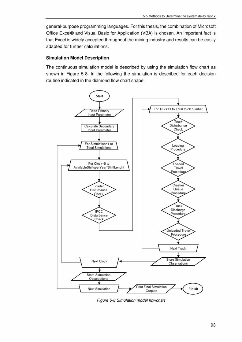
5.5 Methods to Determine the system delay ratio
93
general-purpose programming languages. For this thesis, the combination of Microsoft
Office Excel® and Visual Basic for Application (VBA) is chosen. An important fact is
that Excel is widely accepted throughout the mining industry and results can be easily
adapted for further calculations.
Simulation Model Description
The continuous simulation model is described by using the simulation flow chart as
shown in Figure 5-8. In the following the simulation is described for each decision
routine indicated in the diamond flow chart shape.
Figure 5-8 Simulation model flowchart

CHAPTER 5: SMIPCC Capacity Determination Method
94
Simulation Start for Initialization of Simulation Run
The simulation starts by reading the input parameters including equipment parameters
related to capacity, disturbance behaviour and travel time parameters as listed in Table
5-1. It is assumed that downstream elements of the continuous part of the IPCC system
have the same capacity as the crusher station.
Table 5-1 Simulation input parameters
Primary Input Parameters Unit
Loader Parameters Bucket size [m³]
Coefficient of variation of bucket payload [-] Mean bucket cycle time [s]
Coefficient of variation of bucket cycle time [-] Repair ratio loader [-]
Mean repair time loader [min] Truck Parameters
Rated payload [t] Maximum overload factor [-]
Repair ratio truck [-] Mean repair time truck [min]
Crusher Station Parameters Design capacity [t/h] Hopper Volume [m³]
Number of truck dump points [-] Repair ratio crusher station [-]
Mean repair time crusher station [min] Conveyor Parameters
Repair ratio conveyors [-] Mean repair time conveyors [min]
Spreader Parameters Repair ratio spreader [-]
Mean repair time spreader [min] Travel Time Parameters
Truck travel time loaded [s] Truck travel time unloaded [s]
Coefficient of variation of truck travel time [-] Manoeuvre and spot at the loader [s]
Manoeuvre and unload time at crusher [s] Time Usage Model
Calendar time [h/a] Non-scheduled production [h/a]
External disturbances [h/a] Preventative maintenance [h/a]
Technological Downtimes (Not proportional) [h/a] Shift Duration [h]
Maximum dump block volume [t] Blast volume [t]
Trackshift time [h/trackshift] Blast Delay [h/blast]
Planned Delays [h/shift] Operating Delay Ratio [-]
Material Properties Insitu density [t/m³]
Swell factor [-] Bucket fill factor [-]
Simulation Inputs Total Truck Number [#]
Total Simulation Runs [#]

5.5 Methods to Determine the system delay ratio
95
Based on the primary input parameters the secondary input parameters are calculated which are listed in Table 5-2. Table 5-2 Secondary simulation input parameters
Secondary Input Parameters Unit Equation
Loader Parameters Mean bucket payload [t] (4-17)
Standard deviation of bucket payload [t] (4-20) Standard deviation of bucket cycle time [s] (4-16)
Mean work time loader [min] (4-49) Truck Parameters
Maximum Truck Capacity [t] (4-17) Mean work time truck [min] (4-49)
IPCC Parameters Repair ratio IPCC series system [-] (5-20)
Mean repair time IPCC series system [min] (5-19) Mean work time IPCC series system [min] (5-22)
Travel Time Parameters Standard deviation of truck travel time loaded [s] (4-45)
Standard deviation of truck travel time unloaded [s] (4-45) Time Usage Model
Planned Delays [h/a] (5-7) Material Properties
Loose density [t/m³] (4-18)
Subsequently the simulation loop is initiated. For each simulation run the statistic
observation such as effective operating time, total tonnage, total truck deliveries ect.
are set to zero. In addition, the element operational states are set to “Working”, trucks
position status is set to “In Loader Queue” and an initial element work time is calculated,
just as all other random variable using the inverse transform method [186]. Excel
provides several in-built inverse distribution functions which calculate the abscissa
variable based on a random probability.
Consequently, the annual loop is initiated which is executed for every second of the
year.
Loader Disturbance Check
For each second within one year the loader disturbance check verifies the
“LoaderRepairStatus”. For example, in case the work time of the loader is depleted a
random repair time is calculated based on an exponential distribution and the loader is
set to “In Repair” state. The reverse operation applies when the repair time is over in
which case a new random work time is calculated and the element is set to “Working”
state.
The code of the loader distribution check is shown in Code 5-1.

CHAPTER 5: SMIPCC Capacity Determination Method
96
Code 5-1 Loader disturbance check
If Clock = LoaderWorkTime Then
LoaderRepairTime = -(Application.WorksheetFunction.Ln(RandomNumber) / (1 /LoaderMeanRepairTime) * 60, 0) + Clock
LoaderRepairStatus = "InRepair"
End If
If Clock = LoaderRepairTime Then
LoaderWorkTime = -(Application.WorksheetFunction.Ln(RandomNumber) / (LoaderLamda) * 60, 0) + Clock
LoaderRepairStatus = "Working"
End If
IPCC Disturbance Check
Again, for each second within one year the IPCC disturbance check verifies the
“IPCCRepairStatus”. The same procedure as described for the loader disturbance
check applies. However, in the case of the IPCC disturbance check, each continuous
element of the IPCC system (crusher station, conveyors and spreader) is considered
by applying the principle of reduction of series systems as described in chapter 5.4.
The code of the loader distribution check is shown in Code 5-2.
Code 5-2 IPCC disturbance check
If Clock = IPCCWorkTime Then
IPCCRepairTime = -(Application.WorksheetFunction.Ln(RandomNumber) / (1 / IPCCMeanRepairTime) * 60, 0) + Clock
IPCCRepairStatus = "InRepair"
End If
If Clock = IPCCRepairTime Then
IPCCWorkTime = -(Application.WorksheetFunction.Ln(RandomNumber) / (IPCCLamda) * 60, 0) + Clock
IPCCRepairStatus = "Working"
End If
Truck Loop
Subsequently the truck loop is initiated in which the operational procedures are
processed for each truck. Each individual truck passes through the following states
(Table 5-3):

5.5 Methods to Determine the system delay ratio
97
Table 5-3 Truck states
Truck Status Location
"TravelUnloaded" Haul Road
"InLoaderQueue" At Loader
"Spotting" At Loader
"GettingLoaded" At Loader
"TravelLoaded" Haul Road
"InCrusherQueue" At Crusher Station
"Discharging" At Crusher Station
Truck Disturbance Check
Similar to the disturbance checks for the loader and the continuous part of the IPCC
system, a disturbance check for trucks is also initiated. The disturbance check verifies
if the work time / repair time of a truck is depleted and sets the TruckRepairStatus to
the appropriate setting.
Code 5-3 shows the shortened code for the truck disturbance check
Code 5-3 Truck disturbance check
If Clock = TruckWorkTime(T) Then
TruckRepairTime(T) = -(Application.WorksheetFunction.Ln(RandomNumber) / (1 / TruckMeanRepairTime) * 60, 0) + Clock
TruckRepairStatus(T) = "InRepair"
End If
If Clock = TruckRepairTime(T) Then
TruckWorkTime(T) = -(Application.WorksheetFunction.Ln(RandomNumber) / (TruckLamda) * 60, 0) + Clock
TruckRepairStatus(T) = "Working"
Truckstatus(T) = "TravelUnloaded"
End If
Loader Queue Procedure
Before loading of the truck can commence the truck status is changed to
“InLoaderQueue” as shown in Code 5-4. However, the truck is only positioned in the
loader queue if the unloaded truck unloaded travel time is completed and its truck
status is “TravelUnloaded”.
Code 5-4 Loader queue procedure
If Clock = TruckTraveltimeUnloaded(T) And Truckstatus(T) = "TravelUnloaded" Then
Truckstatus(T) = "InLoaderQueue"
QueueLoader = QueueLoader + 1
End If

CHAPTER 5: SMIPCC Capacity Determination Method
98
Loading Procedure
As soon as the truck is in its final loading position, the loader status is set to “Working”
and the loading procedure is initiated. Loader and truck statuses are changed to
"Loading" and “GettingLoaded” respectively. Then a loading algorithm based on the
equations described in subchapter 4.3.3 and 4.4.1 calculates random truck payloads
and truck loading times.
The loading procedure code is shown in Code 5-5.
Code 5-5 Loading procedure
If Truckstatus(T) = "InLoaderQueue" And LoaderOperationalStatus = "NotLoading" And LoaderRepairStatus = "Working" Then
QueueLoader = QueueLoader - 1
Truckstatus(T) = "GettingLoaded"
LoaderOperationalStatus = "Loading"
Call loadingprocedure
TruckloadingTime(T) = RandomTruckLoadingTime + Clock
TruckPayload(T) = RandomTruckPayload
TotalTonnageLoader = TotalTonnageLoader + TruckPayload(T)
End If
Loaded Travel Procedure
The function of the loaded travel time procedure is to calculate a normally distributed
loaded truck travel time based on mean loaded truck travel time and its standard
deviation.
The code for the loaded travel procedure is shown in Code 5-6.
Code 5-6 Loaded travel procedure
If Clock = TruckloadingTime(T) And Truckstatus(T) = "GettingLoaded" Then
LoaderOperationalStatus = "NotLoading"
Truckstatus(T) = "TravelLoaded"
Call random
TruckTraveltimeLoaded(T) = WorksheetFunction.NormInv(RandomNumber, MeanTruckTraveltimeLoaded, StdTravelTimeLoaded), 0) + Clock
End If
Crusher Queue Procedure
Similar to the loader queue procedure the function of the crusher queue procedure is
to serve a first in first out queue priority in a Single-Queue-Multiple-Service-Points
arrangement.

5.5 Methods to Determine the system delay ratio
99
The code for the crusher queue procedure is shown in Code 5-7.
Code 5-7 Crusher queue procedure
If Clock = TruckTraveltimeLoaded(T) And Truckstatus(T) = "TravelLoaded" And TruckRepairStatus(T) = "Working" Then
Truckstatus(T) = "InCrusherQueue"
QueueCrusher = QueueCrusher + 1
End If
Truck Discharge Procedure
The truck discharge procedures function is to process the discharge of the trucks at
the crusher station. A truck can discharge its payload at one of the dump points of the
crusher station when the sum of current hopper volume and the truck payload does not
exceed the maximum hopper volume, the continuous part of the IPCC system is
working, and a dump point is available. If the conditions are met the truck status
changes to discharging, the crusher station queue is reduced by one truck and the
used dump points are increased by one truck. The truck discharges the material for a
fixed manoeuvre and dump time at the crusher station as described in subchapter
4.4.4. The hopper volume increases by the truck payload and the truck payload
decreases to zero.
The code for the truck discharge procedure is shown in Code 5-8.
Code 5-8 Truck discharge procedure
If Truckstatus(truck) = "InCrusherQueue" And HopperVolume + TruckPayload(T) < HopperCapacity Then
If IPCCRepairStatus = "Working" And UsedDumpPoints < NumberofDumpPoints Then
Truckstatus(T) = "Discharging"
QueueCrusher = QueueCrusher - 1
UsedDumpPoints = UsedDumpPoints + 1
TruckDischargeTime(T) = SpotTimeAtCrusher + Clock
HopperVolume = HopperVolume + TruckPayload(truck)
TruckPayload(T) = 0
End If
End If
Unloaded Travel Procedure
As soon as the truck has finished its discharge procedure the unloaded travel time
procedure is initiated. A normally distributed unladed travel time is calculated by the
mean unloaded truck travel time and the standard deviation. Additionally, the used
dump points are reduced by one truck and the truck status is changed to
“TravelUnloaded”.
The code for the truck discharge procedure is shown in Code 5-9.

CHAPTER 5: SMIPCC Capacity Determination Method
100
Code 5-9 Unloaded travel procedure
If Clock = TruckDischargeTime(T) And Truckstatus(T) = "Discharging" And Then
Truckstatus(T) = "TravelUnloaded"
UsedDumpPoints = UsedDumpPoints - 1
TruckTraveltimeUnloaded(T) = WorksheetFunction.NormInv(RandomNumber, MeanTruckTraveltimeUnloaded, StdTravelTimeUnloaded) + Clock
End If
Finally, the statistical observations are recorded including effective operating time,
unexpected repair time and tonnage processed for the loader and the continuous part
of the IPCC system. Additionally, the average idle time of the trucks is recorded.
Table 5-4 summarizes the various states a system element can obtain. A state or status
represents the condition in which an element is in at a specific point in time.
Table 5-4 Element states
Element Operational State Repair State
Loader Not Loading In Repair
Loading Working
Truck In Loader Queue In Repair
Getting Loaded Working
Travel Loaded
In Crusher Queue
Discharging
Travel Unloaded
Continuous part of IPCC system Not Processing In Repair
Processing Working System Trackshifting
Not Trackshifting Blasting Not Blasting

101
CASE STUDY
In this chapter a case study based on a hypothetical coal mine is conducted. The objective of the case study is to draw descriptive conclusions with regards to annual capacity, productivity and system-induced operating delays of elements in a SMIPCC system.
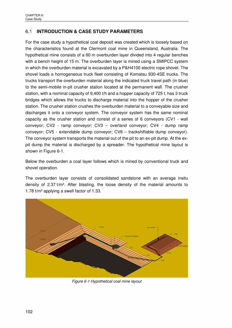
CHAPTER 6: Case Study
102
INTRODUCTION & CASE STUDY PARAMETERS
For the case study a hypothetical coal deposit was created which is loosely based on
the characteristics found at the Clermont coal mine in Queensland, Australia. The
hypothetical mine consists of a 60 m overburden layer divided into 4 regular benches
with a bench height of 15 m. The overburden layer is mined using a SMIPCC system
in which the overburden material is excavated by a P&H4100 electric rope shovel. The
shovel loads a homogeneous truck fleet consisting of Komatsu 930-4SE trucks. The
trucks transport the overburden material along the indicated truck travel path (in blue)
to the semi-mobile in-pit crusher station located at the permanent wall. The crusher
station, with a nominal capacity of 9,400 t/h and a hopper capacity of 725 t, has 3 truck
bridges which allows the trucks to discharge material into the hopper of the crusher
station. The crusher station crushes the overburden material to a conveyable size and
discharges it onto a conveyor system. The conveyor system has the same nominal
capacity as the crusher station and consist of a series of 6 conveyors (CV1 - wall
conveyor; CV2 - ramp conveyor; CV3 – overland conveyor; CV4 - dump ramp
conveyor; CV5 - extendable dump conveyor; CV6 – trackshiftable dump conveyor).
The conveyor system transports the material out of the pit to an ex-pit dump. At the ex-
pit dump the material is discharged by a spreader. The hypothetical mine layout is
shown in Figure 6-1.
Below the overburden a coal layer follows which is mined by conventional truck and
shovel operation.
The overburden layer consists of consolidated sandstone with an average insitu
density of 2.37 t/m³. After blasting, the loose density of the material amounts to
1.78 t/m³ applying a swell factor of 1.33.
Figure 6-1 Hypothetical coal mine layout

6.1 Introduction & Case Study Parameters
103
The hypothetical mine is planned to operate 362 days per annum, allowing 3 days for
non-worked holidays, in two 12 hour shifts per day. It is estimated that the mine stops
operation due to bad weather conditions and other external downtimes for a total of 5
days per year. Preventative maintenance for the continuous part of the IPCC system
is scheduled for 16 hours (4 hours to clean / 12 hours to maintain) every second week.
Furthermore, an annual maintenance shutdown period is planned for 7 days. For the
P&H 4100 the preventative maintenance schedule is planned to commence every
week for 12 hours of which 50% is done in sync with the preventative maintenance for
the continuous part of the IPCC system. By using equation (5-6) the total time for
preventative maintenance ( ) is planned to amount to 896 hours per annum.
For every shift one hour of planned delays are approximated to allow for meal breaks,
equipment inspection and safety rounds. Using equation (5-7) the annual planned shift
delays ( ) are approximated to 640 hours.
Table 6-1 summarizes the relevant loader and truck parameters in order to calculate
the mean hourly loader capacity.
Table 6-1 Loader and truck parameters
Loader and Truck Parameters Unit Value
Loader Parameters Bucket size [m³] 63
Coefficient of variation of bucket payload [-] 0.10 Mean bucket cycle time [s] 33
Coefficient of variation of bucket cycle time [-] 0.20 Bucket fill factor [-] 0.86
Truck Parameters Rated payload [t] 290
Maximum overload factor [-] 1.2
Using equation (4-24), (4-29) and (4-40) the mean truck payload and mean truck
loading time was determined to 291.61 and 111.7 at a mean number
of required bucket cycles 3.023 which leads to a mean hourly loader capacity of
9,398t/h.
291.61 ∙ 3600111.7 9,398 /ℎ The operating delay ratio of the loader was estimated to 0.08 to account for minor
short-term delays such as minor pad preparations, face clean-ups, tramming, etc.
Maximum dump block volume and blast volume were approximated to 2.4 Mm³ and
0.375 Mm³, respectively. The required trackshifting time and blasting time were
estimated to 24 hours and 1.5 hours, respectively. Using equation (5-9) to (5-11) the
technological downtime ratio could be calculated.

CHAPTER 6: Case Study
104
( ) (1,000 ∗ 48 ∗ 50 ) ∗ 1.78 / ³9,398 /ℎ 454ℎ ( ) (500 ∗ 50 ∗ 15 ) ∗ 1.78 / ³9,398 /ℎ 71ℎ
( ) +
( )24ℎ454ℎ + 1.5ℎ71ℎ 0.074 .
The mean truck travel time unloaded and truck travel time loaded were
estimated to 190 s and 290 s, respectively. The coefficient of variation of loaded and
unloaded travel time was estimated to 0.15. In addition, a 45 s manoeuvre and spot
time at the loader and a 60 s manoeuvre and dump time at the crusher was
projected.
The estimated disturbance parameter for the system elements are listed below.
Table 6-2 Disturbance parameters of SMIPCC system elements
Element Disturbance Parameters
Mean repair time [min]
Repair ratio Mean Work Time [min]
Loader 132.7 0.170 782
Truck 288.1 0.128 2251
Crusher Station 33.1 0.117 282
Conveyor
CV1 31.8 0.012 2661 CV2 21.0 0.007 3205
CV3 21.0 0.007 3205
CV4 21.0 0.007 3205
CV5 31.8 0.012 2661
CV6 32.7 0.019 1722
Spreader 52.1 0.059 878
CONDUCTED CALCULATIONS
The following calculations were conducted:
• Calculation 1 – Capacity determination of SMIPCC system for various
truck quantities
• Calculation 2 – Economic analysis
• Calculation 3 – Sensitivity analysis
• Calculation 4 – Introduction of small stockpile in front of crusher station
• Calculation 5 – Comparison to conventional truck and shovel operation

6.2 Conducted Calculations
105
Calculation 1
To analyse the SMIPCC system capacity for various homogenous truck quantities, the
input parameters as specified in section 6.1 were applied to the simulation model
described in section 5.5.2. A total of 1,000 simulations were conducted. Figure 6-2
shows the resulting annual SMIPCC system capacity for various truck quantities.
Figure 6-2 SMIPCC system capacity for various number of trucks
It can be seen that the annual SMIPCC system capacity increases significantly
between 2 and 7 trucks while only minor capacity increases occur between 8 and 14
trucks. For instance, the SMIPCC system capacity increases by 21% from 25.47 Mt/a
to 30.88 Mt/a when employing 5 instead of 4 trucks. However, only 4% of SMIPCC
system capacity is added when employing 8 instead of 7 trucks. Figure 6-3 indicates
the relative change in SMIPCC system capacity for incremental truck number increase.
Figure 6-3 SMIPCC system capacity change for various trucks
The reason for this significant decrease originates from the system delay ratio of the
loader and trucks. Figure 6-4 shows that the system delay ratio for the loader has an
inverse trend compared to the SMIPCC system capacity (Figure 6-2), which indicates

CHAPTER 6: Case Study
106
that the time the loader is ready for operation but is waiting for trucks decreases with
the employed number of trucks in the system. However, the progression of the system
delay ratio of the loader is not linear but rather follows a power function and approaches
a limit of approximately 0.21 at 14 trucks.
Contrary effects are obtained for the system delay ratio of trucks. The more trucks that
are introduced to the system, the more time an individual truck is waiting in front of the
loader or crusher. The progression of the system delay ratio of trucks follows
approximately an exponential function.
Figure 6-4 System Delay Ratios for loader and truck for various number of trucks
Calculation 2
An economic analysis exclusively based on OPEX (Operational Expenditures) was
undertaken in order to identify the optimal number of trucks. Maintenance and power
cost for the P&H 4100 as well as for the 930-4SE were obtained from [187] while the
OPEX cost for the continuous part of the IPCC system (crusher station, conveyors and
spreader), as well as the labour costs for each system element, were estimated by the
author. The OPEX for each system element when idle are based on the labour cost.
Table 6-3 summarises the OPEX parameters of the system elements used for the
analysis.
Table 6-3 OPEX parameters for system elements
OPEX Parameters Unit P&H 4100 930-4SE IPCC
Maintenance Cost (including wear & spear parts, labour, lubrication)
[$/h] 434 312 481
Power/Fuel Cost [$/h] 87 94 387
Labour Cost [$/h] 170 150 500
Total OPEX while operating [$/h] 691 556 1368
Percentage of OPEX while Idle [%] 30% 32% 42%
Total OPEX while Idle [$/h] 205 178 568

6.2 Conducted Calculations
107
Figure 6-5 shows the SMIPCC system capacity, total OPEX and cost per tonne for
various truck quantities. It can be seen that the cost per tonne of the SMIPCC system
decreases by 0.16 $/t between 2 and 6 trucks, where it reaches its minimum at 0.69 $/t
before it increases moderately for the remaining truck quantities.
Figure 6-5 Economic analysis on OPEX
The reason for this trend can be found in the developments of effective operating time
and system-induced operating delay and their associated OPEX for the individual
system elements (refer to Figure 6-6). While the loader and the IPCC system elements
show similar trends for their time components, in which effective operating time
increases and system-induced operating delays decrease as more trucks are
introduced to the system, the time components for the truck show opposite trends.
Figure 6-6 Effective operating time and system-induced operating delays of Loader, Truck and
IPCC

CHAPTER 6: Case Study
108
Calculation 3
To some degree a mining company can influence the mean repair time by improving
the maintenance organisation. This can be realised by ensuring that frequent spare
and wear parts are available at any time, having skilled and experienced maintenance
personnel and necessary tools close to the equipment at all times, and using
equipment fault diagnostics.
A sensitivity analysis was carried out based on 6 trucks to analyse the effects of the
maintenance organisation on SMIPCC system capacity. For each system element the
original mean time for repairs (Table 6-2) was varied between ± 30%.
Figure 6-7 indicates the relative change of SMIPCC system capacity for different mean
time for repairs of system elements.
Generally, the SMIPCC capacity increases as the mean repair time of the system
element decreases. The largest impact on SMIPCC system capacity is the change of
the mean repair time for the continuous part of the IPCC system (crusher station,
conveyors, spreader). By reducing the mean repair time of these elements by 10%,
20% and 30%, an annual capacity increase of the entire SMIPCC system of 4%, 7%
and 11% can be achieved, respectively. Therefore, efforts toward the reduction of the
mean repair time of the continuous part of the SMIPCC promise highest achievement.
Figure 6-7 Sensitivity analysis on mean time to repair
Calculation 4
To analyse the effect of a little stockpile in front of the crusher, additional calculations
were conducted through a minor alteration of the simulation code as described in
section 5.5.2. The alteration of the code is shown in Code 6-1. The modelling of a small
stockpile in front of the crusher station was accomplished by ignoring the following
conditions:
• IPCC Repair Status = "Working" and

6.2 Conducted Calculations
109
• UsedDumpPoints < NumberofDumpPoints
Code 6-1 Truck discharge procedure - alteration
If Truckstatus(truck) = "InCrusherQueue" And HopperVolume + TruckPayload(T) < HopperCapacity Then
Truckstatus(T) = "Discharging"
QueueCrusher = QueueCrusher - 1
UsedDumpPoints = UsedDumpPoints + 1
TruckDischargeTime(T) = SpotTimeAtCrusher + Clock
HopperVolume = HopperVolume + TruckPayload(truck)
TruckPayload(T) = 0
End If
End If
An analysis was carried out based on 6 trucks to analyse the effects of a small stockpile
in front of the crusher station. Therefore, the hopper capacity was gradually increased
from 2,000 t to 18,000 t in 2,000 t intervals.
Figure 6-8 shows the annual SMIPCC capacity for various stockpile capacities. As
expected, the SMIPCC system capacity increases the more that stockpile capacity is
available. However, the progression of the graph indicates that the SMIPCC system
approaches a limit. For example, the results indicate that by introducing an 18,000 t
stockpile (which approximates an area of 95 m by 95 m at a truck dump height of 2 m),
the SMIPCC system capacity can be increased by 5.1 Mt/a in comparison to the base
case.
Figure 6-8 SMIPCC system capacity vs. stockpile capacity
To analyse whether or not the introduction of a stockpile in front of the crusher station
makes economic sense, the cost per tonne based on the parameters specified in Table
6-3 for each case were calculated. Figure 6-9 shows the cost per tonne of the SMIPCC
system for various stockpile capacities. It can be seen that the cost per tonne
decreases as the stockpile capacity increases. Still, the results indicate that the cost

CHAPTER 6: Case Study
110
per tonne for the SMIPCC system can only be reduced by 0.046 $/t (6.7%) compared
to the base case when introducing an 18,000 t stockpile.
It therefore remains questionable whether or not the introduction of a small stockpile in
front of the crusher station is economically advantageous for the following reasons:
• additional equipment such as front end loaders are required to feed the crusher
station with stockpile material at the required feed rate capacity, which means
that additional cost of rehandling material from the stockpile would apply.
• additional space needs to be created in order to accommodate the stockpile,
which might lead to significant increased material movements.
Figure 6-9 Cost per tonne of SMIPCC system for various stockpile capacities
However, the results also indicate diminishing marginal returns. Therefore, even a
small increase of the hopper capacity (which requires no additional equipment) results
in an increase in SMIPCC system capacity and hence in a reduction of cost per tonne.
This occurs because the highest cost per tonne reduction of the SMIPCC system can
be realised by increasing the stockpile capacity from the base case to 2,000 t (Figure
6-10).

6.2 Conducted Calculations
111
Figure 6-10 Reduction of SMIPCC system cost per tonne by stockpile capacity increase
Calculation 5
Further calculations were conducted in order to compare a conventional truck and
shovel system to a SMIPCC system in terms of time usage model and OPEX. To
facilitate this analysis minor alterations of the simulation code as described in section
5.5.2 were required. The modelling of a conventional truck and shovel operation was
accomplished through the following parameter changes:
• IPCCRepairStatus was fixed to „Working" at any time
• NumberofDumpPoints was set to infinity
Additionally, for the conventional truck and shovel system the mean truck travel time
unloaded and truck travel time loaded were increased by a factor of 2.5 to 475 s
and 725 s respectively, in order to account for increased vertical and horizontal travel
distances. Furthermore, the manoeuvre and dump time was reduced to 45 s to account
for easier dumping conditions at the waste dump.
All other input parameters as specified in section 6.1 remained unchanged.
In Figure 6-11 the effective operating time and the system-induced operating delay of
the loader for both competing systems is depicted. It can be seen that the effective
operating time of the conventional truck and shovel system increases approximately
linear from 2 to 14 trucks as the number of trucks increases. Beyond the number of 14
trucks the effective operating time of the conventional truck and shovel system begins
to level off. Furthermore, it can be seen that the SMIPCC system yields higher effective
operating hours per additional truck however it levels off at a lower truck quantity in
comparison to the truck and shovel system. The reverse effects can be seen for the
system induced operating delays of the two systems.

CHAPTER 6: Case Study
112
Figure 6-11 Comparison of effective operating time and system-induced delay of the loader
In Figure 6-12 the effective operating time and the system-induced operating delay of
the trucks (average) for both competing systems is depicted. It should be noted that
the effective operating time of each truck decreases more rapidly with the SMIPCC
system in comparison to the truck and shovel system; as more trucks are introduced
into the system, they experience more wait time rather than effective operating time.
This can be clearly seen in the system-induced operating delays of the trucks in the
SMIPCC system. This effect is not as profound in the conventional truck and shovel
system.
Figure 6-12 Comparison of effective operating time and system-induced delay of the truck
However, despite the increasing ineffectiveness of individual trucks (Figure 6-12), the
annual effective operating hours of the SMIPCC system nevertheless increases more
significantly for each additional truck compared to the conventional truck and shovel
system, up to a certain truck quantity (Figure 6-11). As stated before, this is assuming
the truck travel time for conventional truck and shovel systems is 2.5 times higher than
for SMPICC systems.
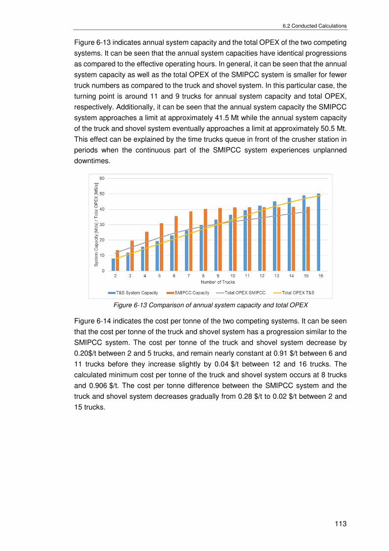
6.2 Conducted Calculations
113
Figure 6-13 indicates annual system capacity and the total OPEX of the two competing
systems. It can be seen that the annual system capacities have identical progressions
as compared to the effective operating hours. In general, it can be seen that the annual
system capacity as well as the total OPEX of the SMIPCC system is smaller for fewer
truck numbers as compared to the truck and shovel system. In this particular case, the
turning point is around 11 and 9 trucks for annual system capacity and total OPEX,
respectively. Additionally, it can be seen that the annual system capacity the SMIPCC
system approaches a limit at approximately 41.5 Mt while the annual system capacity
of the truck and shovel system eventually approaches a limit at approximately 50.5 Mt.
This effect can be explained by the time trucks queue in front of the crusher station in
periods when the continuous part of the SMIPCC system experiences unplanned
downtimes.
Figure 6-13 Comparison of annual system capacity and total OPEX
Figure 6-14 indicates the cost per tonne of the two competing systems. It can be seen
that the cost per tonne of the truck and shovel system has a progression similar to the
SMIPCC system. The cost per tonne of the truck and shovel system decrease by
0.20$/t between 2 and 5 trucks, and remain nearly constant at 0.91 $/t between 6 and
11 trucks before they increase slightly by 0.04 $/t between 12 and 16 trucks. The
calculated minimum cost per tonne of the truck and shovel system occurs at 8 trucks
and 0.906 $/t. The cost per tonne difference between the SMIPCC system and the
truck and shovel system decreases gradually from 0.28 $/t to 0.02 $/t between 2 and
15 trucks.

CHAPTER 6: Case Study
114
Figure 6-14 Comparison of cost per tonne
Figure 6-15 visualises the effect of cost per tonne and annual system capacity of the
two competing systems in more detail. In particular, it can be seen that between an
annual capacity of 14 Mt/a to 41.5 Mt/a, the cost per tonne of the SMIPCC system is
below the cost per tonne of the truck and shovel system. The cost per tonne difference
between the two systems increases gradually from 0.14 $/t to 0.22 $/t for annual
system capacities between 14M t/a and 38 Mt/a, and decrease significantly beyond
40M t/a.
Figure 6-15 Annual system capacity vs. cost per tonne
Figure 6-16 indicated the required number of trucks for various annual system
capacities for the competing systems. It can be seen that the more annual system
capacity is required, the more trucks need to be introduced to each system. However,
up to approximately 40 Mt/a required system capacity the SMIPCC system requires
significantly fewer trucks. In this system capacity range the difference of the required
truck quantity between the truck and shovel system and the SMIPCC system fluctuates
between 1 and 4 trucks.
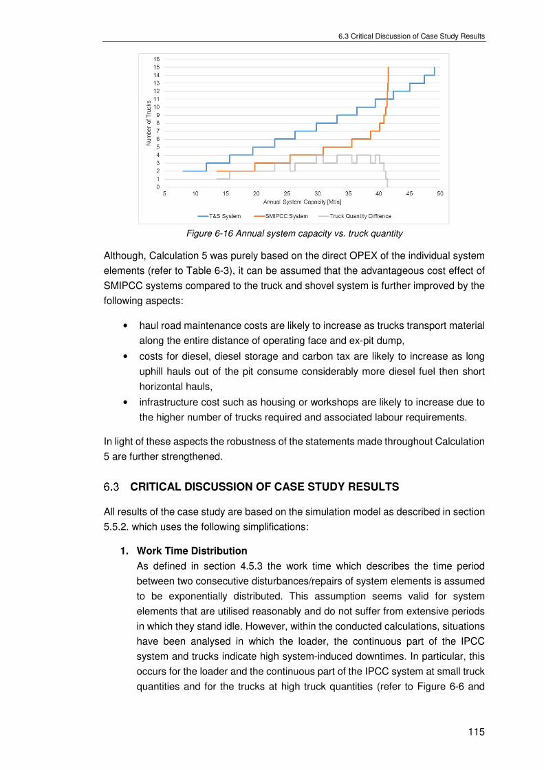
6.3 Critical Discussion of Case Study Results
115
Figure 6-16 Annual system capacity vs. truck quantity
Although, Calculation 5 was purely based on the direct OPEX of the individual system
elements (refer to Table 6-3), it can be assumed that the advantageous cost effect of
SMIPCC systems compared to the truck and shovel system is further improved by the
following aspects:
• haul road maintenance costs are likely to increase as trucks transport material
along the entire distance of operating face and ex-pit dump,
• costs for diesel, diesel storage and carbon tax are likely to increase as long
uphill hauls out of the pit consume considerably more diesel fuel then short
horizontal hauls,
• infrastructure cost such as housing or workshops are likely to increase due to
the higher number of trucks required and associated labour requirements.
In light of these aspects the robustness of the statements made throughout Calculation
5 are further strengthened.
CRITICAL DISCUSSION OF CASE STUDY RESULTS
All results of the case study are based on the simulation model as described in section
5.5.2. which uses the following simplifications:
1. Work Time Distribution
As defined in section 4.5.3 the work time which describes the time period
between two consecutive disturbances/repairs of system elements is assumed
to be exponentially distributed. This assumption seems valid for system
elements that are utilised reasonably and do not suffer from extensive periods
in which they stand idle. However, within the conducted calculations, situations
have been analysed in which the loader, the continuous part of the IPCC
system and trucks indicate high system-induced downtimes. In particular, this
occurs for the loader and the continuous part of the IPCC system at small truck
quantities and for the trucks at high truck quantities (refer to Figure 6-6 and

CHAPTER 6: Case Study
116
Figure 6-11). For those situations when the system element is waiting, it can be
expected that the work time of the element would increase substantially, as the
working intensity is lower in comparison to periods of effective operating time.
Thus, the amount of downtimes would decrease which would lead to an
increase of effective operating time and annual system capacity. The results of
the case study can be assumed to be valid for situations in which the system
element is reasonably utilised.
2. Alteration of Truck Allocation
Based on the simulation model trucks are required to wait in front of the crusher
station whenever a failure or disturbance occurs at the continuous part of the
IPCC system, regardless of the time it requires to be repaired. In reality trucks
would be dispatched directly to the ex-pit dump whenever the identified failure
is expected to take longer than a certain time period. For example, in the case
of a conveyor belt rip the continuous part of the IPCC system can be down for
1 or 2 days. In those situations, trucks would be directly dispatched to the ex-
pit dump which would further increase the effective operating time of the loader
and therefore increase the annual system capacity of the SMIPCC system.
3. Preventative Maintenance for Trucks
In the simulation model it is assumed that the occurrence and duration for
preventative truck maintenance is identical to the preventative maintenance for
other system elements. In reality preventative truck maintenance is based on
regular service intervals determined by Service Meter Unit (or SMU) hours of
the individual truck. This circumstance would lead to periods in which one or
more trucks cannot be utilised which would decrease the result of the annual
system capacity.
4. Trucks in Reserve
The current simulation model does not account for any trucks in cold reserve.
Hartmann [25] suggests that for every five to six production units (trucks), one
spare unit should be provided in order to maintain production. The provision of
spare truck units would further increase the results of the effective operating
time of the loader and therefore increase the annual system capacity.
5. Increasing Truck Travel Times
In the simulation model the truck travel time varies within a certain spread
around the mean which remains constant over the entire observation period.
However, in reality the truck travel time is likely to increase as the operating
face develops further away from the SMIPCC crusher station or the ex-pit dump
area. This circumstance would lead to a slight decrease of the annual system
capacity.

117
SUMMARY AND RECOMMENDATIONS
This chapter presents a brief summary of this research, the accomplishments, and directions for future research.

CHAPTER 7: Summary and Recommendations
118
SUMMARY
During the last decade, the mining industry has developed particular interest in
SMIPCC systems for the transportation of waste rock materials. As the interest for
IPCC systems increases so does the demand for investigative studies to analyse the
applicability. The basis for such investigative studies is the knowledge of achievable
effective operating hours of these systems and their corresponding annual capacity to
meet assigned production schedules. Historically, deterministic calculations based on
empirical data provided merely satisfactory estimates. However, disturbances and
operational variations such as delays and hold-ups are inevitable in any earthmoving,
quarrying and mining operation no matter how well the operation may be planned or
managed. Thus, all too often such traditional calculation methods have proven to be
inadequate in practice and outcomes have not met expectancy. Traditional calculation
methods have four notable shortcomings; they
1. underestimate the influence of the random behaviour of system components
and their interactions,
2. are time consuming when alteration is necessary to suit individual project
requirements,
3. lack in terms of standardization throughout the industry, and
4. systematically carry hazards of human error and under or overestimate the
achievable IPCC system capacities.
Therefore, the objective of this thesis was to develop a structured method to determine
the annual capacity of SMIPCC systems under consideration of the random behaviour
system elements and their interactions with one another. This objective was
accomplished by achieving the following sub-ordinated targets:
1. Comprehensive analysis of in-pit crushing and conveying system (IPCC) and
its applicability to the mining industry.
2. Literature review of available capacity determination methods for continuous
mining systems and more particularly for SMIPCC systems.
3. Description and analysis of random SMIPCC system element behaviour.
4. Description and standardisation of a time usage model applicable to SMIPCC
systems.
5. Development of a simulation model capable of determining system-induced
operating delays.
The following findings of the research can be noted:
An analysis of IPCC systems which have been installed, are currently in
erection/manufacturing process or on order since 1956 over the last seven decades
revealed that in terms of quantity, fixed and fully-mobile systems, increasingly lose
importance on account of semi-mobile and semi-fixed IPCC system. Within the last

7.1 Summary
119
decade 59% of all systems were of semi-mobile or semi-fixed type. Furthermore, it was
found that the installed throughput capacity of all crusher station types increased during
the last decades nevertheless they seem to reach their limits at around 12,000 t/h,
14,000 t/h and 9,000 t/h for fixed, semi-mobile or fully-mobile crusher stations.
Additionally, it was found that with 32% in the last decade the transportation of
overburden material by IPCC systems gains increasingly importance.
The random behaviour of SMIPCC system elements have a significant impact on the
SMIPCC system capacity. They can be distinguished into capacity variation and
disturbance variation. For each SMIPCC system element and their associated unit
operations, adequate distributions have been defined based on available data from
actual mining operations and literature in order to model their behaviour. As the
capacity determining element, strong emphasis is given to the truck loading procedure
of discontinuous loaders.
It was established that bucket payload and truck travel time can be sufficiently
described by a normal distribution, while the bucket cycle time is better approximated
by a gamma distribution. Additionally, it was shown that the truck payload and the truck
loading time depend on the number of identically distributed bucket payloads, the truck
payload policy and the loading methodology implemented at the mine. For both
parameters distribution functions based on a single side loading method and full bucket
policy were developed. Disturbance behaviour such as repair time and work time of
SMIPCC system elements was found to be adequately represented by exponential
distribution.
A time usage model specific for a simplified SMIPCC systems was developed based
on TGL 32 - 778/01-15 which states all essential time components and structures the
time components by their relation to each other. In this thesis, the factor system delay
ratio is introduced, which enables accurate calculation of system-induced operating
delays. Additionally, a simulation model was developed to quantify the system delay
ratio while incorporating the complexity of the whole SMIPCC system, including the
random behaviour of each system element and their interrelated dependencies.
The developed SMIPCC capacity calculation method is used in a case study to analyse
the system behaviour based on a hypothetical mine with regards to time usage model
components, system capacity and cost as a function of truck quantity and stockpile
capacity. The major findings of the case study included the following:
• As expected, the annual capacity of a SMIPCC system increases as more
trucks are introduced to the system. However, the increase of SMIPCC capacity
shows diminishing marginal returns as the number of trucks in the system
increases. Furthermore, the results indicate that annual SMIPCC capacity
approaches a limit. In this particular case study, the limit of the annual SMIPCC
system capacity was approximately 41.5 Mt/a.

CHAPTER 7: Summary and Recommendations
120
• The progression of the cost per tonne curve of a SMIPCC system over an
increasing number of trucks indicates two stages; one in which the cost per
tonne decreases until they reach a minimum and one in which the cost per
tonne increases. The positively sloped portion of the cost per tonne curve is
directly attributable to the diminishing marginal returns of the annual SMIPCC
system capacity. In this particular case study, the minimum cost per tonne of
the SMIPCC system was found at 6 trucks and 0.69 $/t. The corresponding
SMIPCC system capacity for that minimum was 35.6 Mt/a.
• As expected, the annual SMIPCC capacity increases as the mean repair time
of the system elements decreases. However, in this particular case study for 6
trucks the reduction of the mean repair time of the continuous part of the
SMIPCC system indicated the highest increase of SMIPCC system capacity.
For example, by reducing the mean repair time of the continuous part of the
SMIPCC system by 10% the annual capacity of the system increased by 3.6%,
while for the same change of the mean repair time for the loader or the trucks
the system capacity increases only by 1.4% and 1.1%, respectively.
• The introduction of a small stockpile in front of the crusher station increases the
annual SMIPCC system capacity. The annual SMIPCC system capacity
increases as the stockpile capacity increases. However, the SMIPCC system
capacity shows diminishing marginal returns as the stockpile capacity
increases. In this particular case study, an increase of the stockpile capacity
from the base case (normal hopper capacity) of 725 t to 2,000 t indicated an
increased SMIPCC system capacity of 4.0%, while an increase of the stockpile
capacity from the base case capacity to a stockpile capacity of 18,000 t resulted
in an increased system capacity of 14.3%.
Correspondingly, the cost per tonne of the SMIPCC system decreases as the
stockpile capacity increases. For example, by increasing the stockpile capacity
from the base case capacity to a stockpile capacity of 18,000 t, the cost per
tonne of the SMIPCC system is reduced by 0.046 $/t.
• The economic comparison of a conventional truck and shovel system compared
to SMIPCC system revealed a significant cost difference between the two
competing systems. In the annual system capacity range of 14 Mt/a to 38 Mt/a,
the cost per tonne of the SMIPCC system was found to be 0.14 $/t to 0.22 $/t,
lower than the truck and shovel system. The underlying assumption of the case
study was that the truck travel time for the truck and shovel system increases
by a factor of 2.5.
As an overall conclusion, it can be said that the accurate determination of annual
SMIPCC system capacity is challenging due to the complexity of random system
element behaviour and their associated interactions. However, the developed method
provides an effective tool to account for these factors, and furthermore provides the
option of directly comparing SMIPCC systems with conventional truck and shovel

7.2 Recomodations for further reasearch
121
systems. This method should certainly be applied for the projection of new SMIPCC
systems, because the increased level of information provided can contribute valuable
insight to the mining industry. A more precise estimation of achievable annual system
capacity, an optimal number of trucks, and associated overall cost per tonne can be
easily determined.
RECOMODATIONS FOR FURTHER REASEARCH
The presented work successfully fulfilled the research objective, which was to develop
a structured method that allows the estimation of the annual capacity of SMIPCC
systems under consideration of the random behaviour of system elements and their
interaction. However, the boundaries of the developed method and the associated
simulation model are focused on simplified SMIPCC systems. Therefore, an expansion
of the method and associated simulation model, which incorporates heterogeneous
truck fleets and multiple loaders, would pose an interesting challenge for future
research and could be continued hereafter.
Additionally, future research can be focused on the further development of the current
simulation model to incorporate the aspects highlighted in section 6.3.
Furthermore, an equivalent method could be developed that provides the same
functions as the method presented in this thesis in order to cover the entire range of
IPCC systems.
Finally, future research could be focused on the development of a model that includes
the entire life of mine, in order to analyse the economic effects of investment costs
when comparing SMIPCC systems to conventional truck and shovel systems.

References
122
References
[1] H. Goergen, Festgesteinstagebau. Clausthal-Zellerfeld: Trans Tech Publ, 1987.
[2] M. Randolph, “Current Trends in Mining,” in SME Mining Engineering Handbook, 3rd ed., P. Darling, Ed. Society for Mining, Metallurgy, and Exploration, Inc. (SME), 2011, p. 15.
[3] C. Jamasmine, “Belaz launches world’s largest mining dump truck,” Mining.com, Oct-2013.
[4] G. Woodrow, “Benchmarks of performance for truck and loader fleets.,” in Third Large Open Pit Mining Conference, 1992.
[5] E. Bozorgebrahimi, “The Evaluation of Haulage Truck Size Effects on Open Pit Mining,” University of British Columbia, 2004.
[6] H. Lieberwirth, “Economic advantages of belt conveying in open-pit mining,” in Mining Latin America / Minería Latinoamericana, 1st ed., D. C. Bailey, Ed. Springer Netherlands, 1994, pp. 279–295.
[7] J. Fabian, “Cyclic mining systems in Czechoslovakian surface mines,” in Proceedings of International symposium on Off-Highway Haulage in Surface Mines, 1989, pp. 205–209.
[8] G. Mudd, “The Sustainability of Mining in Australia : Key Production Trends and Their Environmental Implications for the Future,” 2009.
[9] J. C. Lucio, C. T. Senra, and A. Souza, “Paving the future – a case study replacing truck-and shovels by shovel-and-conveyor continuous mining at Carajas open pit mines.,” in Iron ore conference 2009, 2009, no. July, pp. 269–276.
[10] R. M. Hays, “Mine Planning Considerations for In-Pit Crushing and Conveying Systems,” in SME Mini Symposium, 1983, pp. 33–41.
[11] E. M. Frizzell, “Mobile In-Pit Crushing - Product of Evolutionary Change,” Trans. Am. Inst. Mining, Metall. Pet. Eng. Soc., vol. 278, no. June, pp. 578–580, 1985.
[12] B. H. Reupke, “Fully mobile in pit crushing and conveying system in ‘Werk Höver.’” Production manager Werk Höver, Holcim, Personal Communication, 2013.
[13] C. Drebenstedt and R. Ritter, “Cyclical and continuous method and in-put crushing operation,” Gornyi Zhurnal, no. 11, pp. 81–87, 2015.
[14] P. Darling, SME mining engineering handbook, vol. 2. Society for Mining, Metallurgy, and Exploration , 2011.
[15] E. Zimmermann and W. Kruse, “Mobile crushing and conveying in quarries-a chance for better and cheaper production!,” in International Symposium Continuous Surface Mining 2006, 2006, pp. 122–129.
[16] P. Moore, “In-Pit Crushing & Conveying – Insights from IPCC 2012,” IM Int. Min., 2012.
[17] R. M. Hays, “Mine Planning Considerations for In-Pit Crushing and Conveying

References
123
Systems,” 1983, pp. 33–41.
[18] D. Turnbull, “A Game Changer in Mining,” Bulk Solids Handling, vol. 33, pp. 16–18, Nov-2013.
[19] J. Korak, “Technisch-wirtschaftliche Untersuchung der Transportbetriebsmittel unter besonderer Berücksichtigung der Transportmittelkombination Fahrbare Brechanlage-Gurtbandanlage für den transport der Haufwerke im engeren Festgesteins-Tagebau,” TU Aachen, 1980.
[20] I. E. Hugo and R. Bunduwongese, “Mobile Crushing/Sizing Systems for Modern Open Cast Mining - A Case Study of Mae Moh Phase 5 Project, Thailand,” in Large Open Pit Conference, 2007.
[21] D. Mac Phail, “The choice between in-pit crushing and conveying and conventional trucking at Valley Copper,” in The Planning and Operation of Open-Pit and Strip-Mines, 1984.
[22] M. Johnson and J. Hoang, “Impacts of IPCC on Pit Shell Optimisation,” in International IPCC Conference, 2014.
[23] D. G. Carmichael, Engineering queues in construction and mining. Ellis Horwood, 1987.
[24] J. Elbrond, “Calculation Of An Open Pit Operation’s Capacity,” in SME Fall Meeting and Exhibit, 1977.
[25] H. L. Hartman, Ed., SME Mining Engineering Handbook, no. Bd. 1. Colorado USA: Society for Mining, Metallurgy, and Exploration, 1992.
[26] J. G. Londono, P. Knights, and M. Kizil, “Review of In-pit Crusher Conveyor (IPCC) application,” in 2012 Australian Mining Technology Conference, 2012, pp. 63–82.
[27] R. A. Beatty and A. A. Bustos-Ramirez, “Dragline Modifications and Hopper Design Associated with the DHCC Method of Open Cut Stripping,” in Third International Conference on Bulk Materials, Storage, Handling and Transportation: Preprints of Papers, 1989, p. 154.
[28] J. G. Londoño, P. F. Knights, and M. S. Kizil, “Modelling of In-Pit Crusher Conveyor alternatives,” Min. Technol., vol. 122, no. 4, pp. 193–199, Dec. 2013.
[29] Fortescue Metals Group, “Chichester Hub,” 2015. [Online]. Available: http://www.fmgl.com.au/Our_Business/Chichester_Hub. [Accessed: 20-Feb-2015].
[30] Sandvik, “Fully-mobile crusher stations for mining operation right for quarry operation.” 2013.
[31] KruppRobins, “Large Capacity Mobile Crushing Plants,” 2014. [Online]. Available: http://www.krupprobins.com/images/Crushers/MobCrush-05.jpg.
[32] Joy Global, “Case Study How In-Pit Crusher Conveyor System Helps PRB Wyodak Coal Mine Sustain Efficient Power Generation,” 2011.
[33] R. W. Utley, “In-Pit Crushing,” in SME Mining Engineering Handbook, 3rd ed., P. Darling, Ed. Society for Mining, Metallurgy, and Exploration, 2011, pp. 941–957.

References
124
[34] R. D. Stoll, C. Niemann-Delius, C. Drebenstedt, and K. Müllensiefen, Der Braunkohlentagebau: Bedeutung, Planung, Betrieb, Technik, Umwelt. Springer, 2008.
[35] J. Plattner, “History and design of mobile in-pit crushers for open pit mines,” Large Open Pit Mining Conference. Australasian Institute of Mining & Metallurgy, Newman, Australia, pp. 17–21, 1986.
[36] S. J. Kirk, Western Surface Coal Mining. Gillette, 1989.
[37] P. Plattner, “Hopper size.” Lead Engineer, Sandvik, Personal Communication, 2012.
[38] Sandvik, “CR800 series hybrid,” 2014. [Online]. Available: http://mining.sandvik.com/sandvik//S003713.nsf/Alldocs/Products*5CCrushers*and*screens*5CRoll*crushers*2ACR810/$file/CR800_hybrid_low_res.pdf.
[39] FLSmidth, “EV hammer impact crusher,” 2014. [Online]. Available: http://www.flsmidth.com/~/media/Brochures/Brochures for crushers and raw material stores/EVHammerImpactCrusherlowres.ashx.
[40] FLSmidth, “Gyratory crushers,” 2014. [Online]. Available: http://www.flsmidth.com/~/media/PDF Files/Crushing/Gyratory Crusher/GyratoryCrusher_brochure.ashx.
[41] ThyssenKrupp, “Gyratory Crusher,” 2014. [Online]. Available: http://www.thyssenkrupp-industrial-solutions.com/fileadmin/documents/brochures/kreiselbrecher_en.pdf.
[42] Pennsylvania and Crusher, “Handbook of Crushing,” 2003. [Online]. Available: https://eva.fing.edu.uy/pluginfile.php/64897/mod_folder/content/0/handbook_of_crushing.pdf?forcedownload=1.
[43] MMD, “MMD SIZERS,” 2014. [Online]. Available: http://www.mmdsizers.com/downloads/MMD_P_A_3_English.pdf.
[44] FLSmidth, “TST jaw crusher,” 2014. [Online]. Available: http://www.flsmidth.com/~/media/PDF Files/Crushing/FLSmidth_TST_JawCrusher_brochure.ashx.
[45] K. Boyd and R. W. Utley, Mineral Processing Plant Design, Practice, and Control Proceedings, no. Bd. 1. Society for Mining, Metallurgy, and Exploration, 2002.
[46] F. Habashi, “A short history of mineral processing,” Proc. XXIII Int. Miner. Process. …, 2006.
[47] M. Harcus, “Crusher Time,” Mining Magazine, London, pp. 48–57, Apr-2011.
[48] Scheuerle, “Self-Propelled Modular Transporters,” 2013. [Online]. Available: http://www.scheuerle.de/en/home/press/article/print.html.
[49] F. Foti, “TIl ,” IPCC 2013. Cologne, 2013.
[50] K. Strzodka, Tagebautechnik. 2, vol. 2. Dt. Verlag für Grundstoffindustrie, 1980.
[51] A. Kesimal, “Different Types of Belt Conveyors and Their Applications in Surface Mines,” Miner. Resour. Eng., vol. 6, no. 04, pp. 195–219, 1997.

References
125
[52] K. J. Benecke and R. S. Shehata, “Application criteria for conveyors in hard rock mining: the system crusher—conveyor—spreader (November 7–8, 1985) Mining Equipment Selection Symp,” Krupp Ind. GmbH, West Ger. CANMET, UK, pp. 1–25, 1985.
[53] E. Bahke, “New developments of belt conveyor systems,” ZKG Int., vol. 45, no. 3, pp. 121–130, 1992.
[54] FAM, “Belt wagons,” 2014. [Online]. Available: http://www2.fam.de/english/Products/Opencast mining systems/Belt wagons/index.html.
[55] TNT, “Convetional horizontal conveyor,” 2014. [Online]. Available: http://www.tntinc.com/grasshopperhorizontalconveyor.html.
[56] Takraf, “Mobile transfer Conveyors,” 2014. [Online]. Available: http://www.takraf.com/en/Products/Mining_Equipments/mobiletransferconveyor.htm.
[57] Sandvik, “Sandvik offering guide 2013-14.” Sandvik, 2014.
[58] J. Kempas, “Application of mobile primary crushing and belt conveying systems for Iron Ore mining,” Australas. Inst. Min. Metall. Publ. Ser., no. August, pp. 311–317, 2007.
[59] G. Grant M., “ADVANCEMENT OF MOBILE CONVEYING SOLUTIONS FOR IPCC AND WASTE HANDLING OPERATIONS ,” IPCC 2013. Cologne, 2013.
[60] Metso, “Nordberg mobile conveyors,” 2014. [Online]. Available: http://www.metso.com/miningandconstruction/mm_conv.nsf. [Accessed: 12-Feb-2014].
[61] Maats, “Trackshifting Dozer.” [Online]. Available: http://www.maats.com/various/liebherr-conveyor-shifters/liebherr-rl-64-conveyor-belt-shifter. [Accessed: 24-Apr-2014].
[62] FAM, “Drive Station,” 2014. [Online]. Available: http://www.fam.de/www.fam.de/english/Products/Conveying/html. [Accessed: 12-Feb-2014].
[63] KruppRobins, “Shiftable Conveyors.” [Online]. Available: http://www.krupprobins.com/Products/Mining Equipment/shiftableconveyors.html. [Accessed: 21-Mar-2014].
[64] J. A. Dos Santos, “Sandwich Belt High Angle Conveyor Applications in Open-Pit Mining,” no. October 1983, 1985.
[65] J. Dos Santos, “High Angle Conveyors-HAC’s from Mine to Prep Plant and Beyond,” Bulk Solids Handl., vol. 13, p. 303, 1993.
[66] E. Sheshko and A. Kutenkov, “Substantiation of parameters high angle conveyor with boards and partitions at large productivity in open cast mines,” Transp. i logistika, 2001.
[67] T. Ziller and P. Hartlieb, Fördergurte in der Praxis: Know How und Know Why ; Fördergurt Herstellung, Montage und Verbindungstechnik, Inspektion, Wartung und Instandsetzung, Maschinen, Hilfs- und Prüfmittel, Wirtschaftlichkeit und Kostenkontrolle, Ressourcenschonung und Umweltschut. VGE-Verlag, 2010.

References
126
[68] J. Weissflog, “Shiftable Belt Conveyor Systems in Open Pit Mining,” SME-AIME Fall Meeting and Exhibit. SME, Utah, USA, 1983.
[69] K. Strzodka, Tagebautechnik. 2, vol. 2. Dt. Verlag für Grundstoffindustrie, 1980.
[70] B. Küsel, “St 10,000 – a new development in high-tension conveyor belt design,” Aust. Bulk Handl. Rev., 2012.
[71] R. Summerford, “Mechanical Splicing vs Vulcanisating,” World Coal, 2009.
[72] G. N. Kunze, H. G. Hring, and K. Jacob, Baumaschinen: Erdbau- Und Tagebaumaschinen, no. Bd. 10. Vieweg+Teubner Verlag, 2002.
[73] P. Plattner, “Spreader Design.” Lead Engineer, Sandvik, Personal Communication, 2014.
[74] Takraf, “Bandabsetzer,” 2014. [Online]. Available: http://www.takraf.com/de/produkte/Tagebauanlagen/Bandabsetzer.htm. [Accessed: 12-Feb-2014].
[75] FAM, “Absetzer auf Raupen,” 2014. [Online]. Available: http://www.fam.de/deutsch/Produkte/Tagebautechnik/Absetzer%2520auf%2520Raupen/index.html. [Accessed: 12-Feb-2014].
[76] ThyssenKrupp, “Spreader References.” ThyssenKrupp Fördertechnik GmbH, 2012.
[77] J. F. Rodenberg, S. . R. Winzer, and D. J. Nordin, “Direct dumping mining systems – Application and economics,” Int. J. Surf. Mining, Reclam. Environ., vol. 2, no. 4, pp. 193–208, Jan. 1988.
[78] FLSmidth, “Mobile Stacking Conveyor,” 2014. [Online]. Available: http://www.flsmidth.com/en-us/Industries/Categories/Products/Material+Handling/Belt+Conveying/MobileConveyorSystems/MobileStackingConveyors. [Accessed: 12-Feb-2014].
[79] FAM, “Stacker,” 2014. [Online]. Available: http://www.fam.de/english/Products/Stockyard%2520systems/Stackers/index.html. [Accessed: 12-Feb-2014].
[80] ThyssenKrupp, “ThyssenKrupp Robins - References,” 2013. [Online]. Available: http://www.thyssenkrupprobins.com/References/Stackers/stackers.html. [Accessed: 12-Feb-2014].
[81] TNT, “Mobile stacking systems,” 2014. [Online]. Available: http://www.tntinc.com/mobilestackingsystemsvideo.html. [Accessed: 12-Feb-2014].
[82] FLSmidth, “Mobile Bridge Boom Stacker,” 2014. [Online]. Available: http://www.flsmidth.com/en-US/Industries/Categories/Products/Material+Handling/Tailings+Waste+Stacking+Systems/MobileBridgeBoomStacker. [Accessed: 12-Feb-2014].
[83] FAM, “Stacker reclaimers,” 2014. [Online]. Available: http://stacker-reclaimer.fam.de/. [Accessed: 12-Feb-2014].
[84] TAKRAF, “Stacker/Reclaimer,” 2014. [Online]. Available: http://www.takraf.com/en/products/yardequipment/stacker_reclaimer.htm.
References
127
[Accessed: 12-Feb-2014].
[85] Liebherr, “Stacker / Reclaimer machines,” 2014. [Online]. Available: http://www.liebherr.com/CP/en-GB/products_cp.wfw/id-18224-0. [Accessed: 12-Feb-2014].
[86] TAKRAF, “Stacker / Reclaimers,” 2014. [Online]. Available: http://www.tenovagroup.com/stacker_reclaimers.php. [Accessed: 12-Feb-2014].
[87] H. G. Kok, “Use of Mobile Crushers in the Minerals Industry,” T 272, ME Nov, vol. 1584, 1982.
[88] D. Wood, W. H. Bryan, and S. of E. Geologists, “Crucial Challenges to Discovery and Mining – Tomorrow’s Deeper Ore Bodies ,” 2012.
[89] G. J. Klir, Trends in general systems theory. John Wiley & Sons Canada, Limited, 1972.
[90] D. König, J. Sajkiewicz, and D. Stoyan, Leistungsberechnung für Fördersysteme. Leipzig: Deutscher Verlag für Grundstoffindustrie, 1985.
[91] J. Sajkiewicz, “Application of numerical symbols for determination of technically possible work states for machinery system,” Exploit. Probl. Mach., vol. 10, no. 22, pp. 219–236, 1975.
[92] G. Gruschka and H. Stoyan, “Planungsmodelle für ein Grubenbetrieb mit Bandförderung und Parallelabbau,” Neue Bergbautechnik, vol. 3, no. 5, pp. 174–177, 1975.
[93] Y. Xi and T. Yegulalp, “Reliability-based capacity determination of a bucket wheel excavator system in Yuabaoshan Surface Coal Mine,” Soc. Min. Eng. AlME, vol. 294, pp. 1953–1959, 1994.
[94] P. Ryder, “Developments in the design, planning and operation of underground conveyor coal belt clearance,” Oper. Res. und Datenverarbeitung im Bergbau, no. 4, p. Y–I1–YI14, 1975.
[95] K. Talbot, “Simulation of conveyor belt networks in coal mines,” in 15th International Symposium APCOM, 1977, pp. 297–304.
[96] J. M. Czaplicki, Shovel-Truck Systems: Modelling, Analysis and Calculations. Taylor & Francis, 2008.
[97] S. Deshmukh, Sizing of Fleets in Open Pits, XXII. American Institute of Mining, Metallurgical and petroleum Engineers, 1970.
[98] E. Koenigsberg, “Cyclic Queues,” Oper. Res., vol. 9, no. 1, pp. pp. 22–35, 1958.
[99] M. J. Maher and J. G. Cabrera, “The transident behavior of cyclic queue,” Oper. Reasearch Q., vol. 24, no. 4, pp. 32–41, 1973.
[100] M. J. Maher and J. G. Cabrera, “A multi-stage cyclic queueing model,” Int. J. Prod. Res., vol. 13, no. 3^603–613, 1975.
[101] P. K. Muduli, “Modeling truck-shovel systems as multiple-chain closed queuing networks,” Columbia University, 1997.

References
128
[102] J. M. Czaplicki, “The analysis and calculation procedure for shovel-truck systems with crusher and conveyor,” Gospod. Surowcami Miner., vol. 24, no. 4/3, 2008.
[103] P. Morriss, “Key Production Drivers in In-Pit Crushing and Conveying (IPCC) Studies,” South. African Inst. Min. Metall., p. 33, 2008.
[104] S. Peng, D. Zhang, and Y. Xi, “Computer simulation of a semi-continuous open-pit mine haulage system,” Int. J. Min. Geol. Eng. Int. J. Min. Geol. Eng., vol. 6, no. 3, pp. 267–271, Oct. 1988.
[105] B. Kolonja, R. Stanić, and J. Hamović, “Simulation of mine material handling systems using AutoMod,” Transp. i logistika, 2001.
[106] M. C. Albrecht, “Equipment sizing of a material handling system using discrete event simulation,” in Application of Computers and Operations Research in the Mineral Industry, Taylor & Francis, 2005, pp. 449–455.
[107] J. Zhang and Q. Wang, “A Queuing Network Model for Shovel-Truck-Crusher Systems in Open-pit Mining,” in Proceedings of Application of Computers and Operations Research in the Mineral Industry Conference 2009, 2009.
[108] R. Todt, “Analyse von Zugmangelzeiten, die durch gegenseitige Beeinflussung der Betriebsabschnitte Gewinnung, Förderung und Verkippung in Abraumabteilungen von Tagebauen mit Zugförderung entstehen,” Dissertation, Technische Universität Bergakademie Freiberg, 1964.
[109] B. Kahn, “Untersuchung zur Anwendung der Technologie der kombinierten Zug-Band-Förderung in Abraumbetrieben von Braunkohlentagebauen Unter bes. Berücks. d. stationären Kippgrabens als Massenspeicher,” [s.n.], Freiberg, 1966.
[110] R. J. Barnes, M. S. King, and T. B. Johnson, “Probability Techniques For Analyzing Open Pit Production Systems,” in Proceedings of the 16th APCOM, 1979, pp. 462–476.
[111] N. R. Billette, “Haulage System Capacity: Analytical and Simulation Models Revisited,” in 19th International Symposium 1986 - Application of Computers and Operations Research, 1986, pp. 355–364.
[112] D. C. Montgomery, Applied Statistics and Probability for Engineers 6th edition: 2013.
[113] C. Burt and L. Caccetta, “Equipment Selection for Surface Mining: A Review,” Interfaces (Providence)., vol. 44, no. 2, pp. 143–162, 2014.
[114] R. J. Hardy, “Selection Criteria For Loading and Hauling Equipment - Open Pit Mining Applications,” Western Australian School of Mines, 2007.
[115] G. Kühn, “Über die Ausnutzung der Universalbagger,” Fördern und Heb., vol. 1, no. 5, pp. 16–21, 1955.
[116] M. Osanloo, “Prediction of Shovel Productivity in the Gol-e-Gohar Iron Mine,” J. Min. Sci., vol. 41, no. 2, pp. 177–184, 2005.
[117] S. P. Singh and R. Narendrula, “Factors affecting the productivity of loaders in surface mines,” Int. J. Mining, Reclam. Environ., vol. 20, no. 1, pp. 20–32, Mar. 2006.
References
129
[118] J. Walenzyk, “Application Engineer, Komatsu Mining Germany GmbH - Excavator productivity.” Düsseldorf, 2014.
[119] H. Härtig, R. Ciesielski, K. Strzodka, and R. Steinmetz, Grundlagen für die Berechnung von Tagebauen. Braunkohle, Kiessand, Ton, Naturstein, 3.Edition ed. Leipzig: Deutscher Verlag für Grundstoffindustrie, 1982.
[120] Harnischfeger, “Peak Performance Practices.” P&H Mining Equipment, Milwaukee, Wisconsin USA, 2003.
[121] W. Schwate, “Beitrag zur optimalen gestalltung der Gewinnung in Festgesteinstagebauen unter besonderer Berücksichtigung der gleislosen diskontinuierlichen Förderung,” TU Freiberg, 1976.
[122] K. Awuah-Offei, B. Osei, and H. Askari-Nasab, “Modeling Truck-Shovel Energy Efficiency under Uncertainty,” in Transactions for the Society for Mining, Metallurgy, and Exploration, Inc. Volume 330, 2011, pp. 573–585.
[123] C. Rowlands and G. D. Just, “Performance Characteristics of Dragline Buckets,” in Third Large Open Pit Mintng Conference, 1992, no. September, pp. 89–92.
[124] E. K. Chanda and R. J. Hardy, “Selection Criteria for Open Pit Production Equipment – Payload Distributions and the ‘10/10/20’ Policy,” in 35th APCOM Symposium 2011, 2011, no. September, pp. 24–30.
[125] P. Knights and S. Paton, “Payload variance effects on truck bunching,” in Seventh Large Open Pit Mining Conference, 2010, no. July, pp. 27–28.
[126] Caterpillar, “Caterpillar Quarry and Construction Truck 10/10/20 Payload Managment Guidelines,” Peoria, USA, 2008.
[127] P&H, “Electric Mining Shovels - Product Overview,” 2014. [Online]. Available: http://www.phmining.com/MinePro/Literature/Brochures/EN-EMS01_brochure.pdf. [Accessed: 23-Oct-2014].
[128] Komatsu, “960E-1K,” 2014. [Online]. Available: http://www.komatsu.com/ce/products/pdfs/KAC_960E-1K.pdf. [Accessed: 23-Oct-2014].
[129] R. W. Barbaro, “Evaluating the productivity of a shovel-truck materials haulage system using a cyclic queueing model,” in AIME Transactions Volume, 1988, vol. 44, no. 2.
[130] J. Maran and E. Topuz, “Simulation of truck haulage systems in surface mines,” Int. J. Surf. Mining, Reclam. Environ., vol. 2, no. 1, pp. 43–49, Jan. 1988.
[131] W. C. Morgan and L. Peterson, “Determining shovel-truck productivity,” Min. Eng., vol. 20, no. 12, pp. 76–80, 1968.
[132] N. K. Nanda, “Optimizing of mine production system through operation research techniques,” in 19th Mining Congress, 2003, pp. 583–596.
[133] G. N. Panagiotou, “Optimizing the shovel-truck operation using simulation and queueing models,” in Proceedings of the Second International Symposium on Mine Mechanization and Automation, Lulea, Sweden, 1993.
[134] Y. Lizotte, E. Bonates, and A. Leclerc, “Analysis of truck dispatching with dynamic heuristic procedures,” in International Symposium on Off-highway
References
130
haulage in surface mines, 1989, pp. 47–55.
[135] J. Szymanski, R. Suglo, S. Planeta, and J. Paraszczak, “Simulation analysis model of mining methods,” in Thirteenth International Symposium on Mine Planning and Equipment Selection, 2004, pp. 613–618.
[136] Y. Lizotte and E. Bonates, “Truck and shovel dispatching rules assessment using simulation,” Min. Sci. Technol., vol. 5, no. 1, pp. 45–58, May 1987.
[137] G. Griffin, “Permutation theory applied to truck-shovel system simulation,” in Off-Highway Haulage in Surface Mines, 1989, pp. 83–87.
[138] L. Zhongzhou, L. Qining, and R. Singhal, “Erlangian cyclic queueing model for shovel-truck haulage systems,” in Mine Planning and Equipment Selection, 1988, pp. 423–428.
[139] B. Knights, M. Kizil, and W. Seib, “Truck-shovel fleet cycle optimisation using GPS collision avoidance system,” in 12th Coal Operators’ Conference, 2012, pp. 361–370.
[140] D. Scheffler and W. Kunze, “Beitrag zur Kapazitätseinschätzung des Kalksteintagebaus Karsdorf,” Neue Bergbautechnik, vol. 2, no. 7, pp. 486–492, 1972.
[141] G. Lumley, “Reducing the Variability in Dragline Operator Performance,” in Coal Operators’ Conference, 2005, pp. 97–106.
[142] D. Stoyan, “Truck loading time modeled as inverse Gaussian distribution.” Freiberg, 2014.
[143] Q. Wang, Y. Zhang, C. Chen, and W. Xu, “Probability distribution of key time parameters in open-pit mine truck dispatching,” J. China Coal Soc., vol. 31, no. 6, pp. 761–764, 2006.
[144] R. A. Carter, “Cat Refines, Expands Rope Shovel Feature Lineup,” Engineering and Mining Journal, 2014.
[145] Tasman Asia Pacific, “Benchmarking the productivity of Australia’s black coal industry,” 1998. .
[146] V. I. Rotar, Probability and Stochastic Modeling. Taylor & Francis, 2012.
[147] D. Stoyan and H. Stoyan, Mathematische Methoden in der Operationsforschung: Fördertechnik, Bergbau, Transportwesen. Deutscher Verlag für Grundstoffindustrie, 1971.
[148] K. Awuah-Offei, B. A. Osei, and H. Askari-Nasab, “Improving Truck-Shovel Energy Efficiency Through Discrete Event Modeling,” in SME Annual Meeting, 2012, p. Preprint 12–069.
[149] D. Gove and W. Morgan, “Optimizing truck-loader matching,” Int. J. Rock Mech. Min. Sci. Geomech., vol. 32, no. 3, 1995.
[150] R. M. Hays, Surface Mining. Littleton CO USA: Society for Mining, Metallurgy, and Exploration, 1990.
[151] Caterpillar, Caterpillar Performance Handbook 42, 42nd ed. Peoria, USA: Caterpillar Inc., 2012.

References
131
[152] S. Gladysz, “Störprozesse in technologischen Systemen der Tagebaue,” Wegiel brunatny, no. 1, pp. S.62–74, 1964.
[153] A. Bovas and L. Johannes, Statistical Methods for Forecasting. New York: Wiley, 1983.
[154] R. a. Hall and L. K. Daneshmend, “Reliability Modelling of Surface Mining Equipment: Data Gathering and Analysis Methodologies,” Int. J. Surf. Mining, Reclam. Environ., vol. 17, no. 3, pp. 139–155, Sep. 2003.
[155] V. A. Temeng, “Probabilistic analysis of reliability and effectiveness of elementary shovel-truck system at Nchanga Open-pit,” University of Zambia, 1988.
[156] G. Sharma, T. Haukaas, R. a. Hall, and S. Priyadarshini, “Bayesian statistics and production reliability assessments for mining operations,” Int. J. Mining, Reclam. Environ., vol. 23, no. 3, pp. 180–205, Sep. 2009.
[157] S. Elevli, N. Uzgoren, and M. Taksuk, “Maintainability analysis of mechanical systems of electric cable shovels,” J. Sci. …, 2008.
[158] R. Hall, “Analysis of Mobile Equipment Maintenance Data In an Underground Mine,” 1997.
[159] F. Simon, B. Javad, and B. Abbas, “Availability analysis of the main conveyor in the Svea Coal Mine in Norway,” Int. J. Min. Sci. Technol., vol. 24, no. 5, pp. 587–591, Sep. 2014.
[160] J. Barabady and U. Kumar, “Reliability analysis of mining equipment: A case study of a crushing plant at Jajarm Bauxite Mine in Iran,” Reliab. Eng. Syst. Saf., vol. 93, no. 4, pp. 647–653, Apr. 2008.
[161] E. Bozorgebrahimi, “The evaluation of haulage truck size effects on open pit mining,” University of British Columbia, 2004.
[162] R. Pascual, R. Madariaga, G. Santelices, D. Godoy, and E. L. Droguett, “A structured methodology to optimise throughput of production lines,” Int. J. Mining, Reclam. Environ., pp. 1–12, Sep. 2014.
[163] J. G. Londono, “Systems modelling of parallel conveyors in IPCC systems,” The University of Queensland, 2012.
[164] J. M. Czaplicki, Statistics for Mining Engineering. Leiden: CRC Press/Balkema, 2014.
[165] J. Sajkiewicz, “Theory der Fördersysteme,” Wrocław, 1980.
[166] CIM, “CIM Mining Standards and Guidelines Committee,” 2012.
[167] Z. Lukacs, “Standard definitions for the benchmarking of availability and utilization of equipment,” 2014.
[168] P. Morriss, “Key Production Drivers in in-Pit Crushing and Conveying (Ipcc) Studies,” South. African Inst. Min. Metall., p. 33, 2008.
[169] P. F. Knights and P. Oyanader, “Best-in-class maintenance benchmarks in Chilean open pit mines,” CIM Bull., vol. 98, no. 1088, p. 93, 2005.

References
132
[170] Xstrata, “XCN BD GDL 0027 TIME MODEL – NOMENCLATURE AND KEY PERFORMANCE INDICATORS.” Xstrata Coal, p. 28, 2014.
[171] M. Dalryple, “Personal Comunication: Time usage model Rio Tinto.” 2014.
[172] TGL 32 - 778/01-15, Begriffe für den Tagebau. Gliederung der Kalenderzeit für Tagebaugeräte. GDR, 1983.
[173] Z. Pan, “Personal Comunication with maintenance manager: Downtime due to bad weather at Zhahanaoer Mine - Houlinhe coal mine company.” 2013.
[174] C. Hu, “Personal Comunication with maintenance manager: Downtimes at Yiminhe Coal Mine -Huaneng Yimin Coal Electricity Corp.” 2013.
[175] P. D. Tomlingson, Mine Maintenance Management Reader. Society for Mining, Metallurgy, and Exploration, 2007.
[176] B. S. Dhillon, Mining Equipment Reliability, Maintainability, and Safety, vol. null. 2008.
[177] P. D. Tomlingson, Equipment Management: Key to Equipment Reliability and Productivity in Mining. Society for Minig, Metallurgy, and Exploration, 2009.
[178] M. Gellrich, “Personal Comunication: Maintenance intervalls BWE system at Vattenfall.” 2014.
[179] D. P. Tripathy, “Effective maintenance Practices for Mining Equipments,” 2011.
[180] R. Ritter, A. Herzog, and C. Drebenstedt, “Automated Dozer Concept Aims to Cut IPCC Downtime,” Engineering & Mining Journal, Jacksonville, pp. 56–59, Nov-2016.
[181] R. Ritter, “Reliability and Capacity Planning of Fully Mobile IPCC Systems,” in International IPCC Conference, 2014.
[182] C. H. Ta, A. Ingolfsson, and J. Doucette, “A linear model for surface mining haul truck allocation incorporating shovel idle probabilities,” Eur. J. Oper. Res., vol. 231, no. 3, pp. 770–778, 2013.
[183] B. V. Gnedenko, Y. K. Belayev, and A. D. Solovyev, Mathematical methods of reliability theory. New York: Academic Press, 1969.
[184] H. Daduna, R. Krenzler, R. Ritter, and D. Stoyan, “Heuristic Approximations for Closed Networks : A Case Study in Open-pit Mining,” Vor. auf arXiv.org, pp. 1–41, 2016.
[185] F. Soumis, J. Ethier, and J. Elbrond, “Truck dispatching in an open pit mine,” Int. J. Surf. Mining, Reclam. Environ., vol. 3, no. 2, pp. 115–119, 1989.
[186] D. Elizandro and H. Taha, Performance Evaluation of Industrial Systems: Discrete Event Simulation in Using Excel/VBA, Second Edition. Taylor & Francis, 2012.
[187] Mine and Mill Equipment Costs. Washington: InfoMine USA, Inc., 2015.
[188] S. N. Chiu, D. Stoyan, W. S. Kendall, and J. Mecke, Stochastic Geometry and Its Applications. Wiley, 2013.

Appendices
133
Appendices
List of Appendices
Appendix I - List of IPCC Systems ....................................................................... 134
Appendix II - Mathematical Proof of Equation (4-11) .......................................... 159
Appendix III - Bucket Cycle Times Data .............................................................. 160
Appendix IV - Repair Time Data ........................................................................... 160

Appendices
134
Appendix I - List of IPCC Systems
Table A-I Global list of IPCC systems
Mine Name Company Name Country Region Commodity
Transported
material
Type of
crusher Type of Feeder
Transport
system Station service
weight [t] Mobility
Number
Modules
Year of
commissioning Systems
Capacity [t/h]
Manufacturer
of System
Crusher
Power [kW]
Sentinel Mine (No.3)
Kalumbila Minerals
Ldt. (First Quantum
Minerals)
Zambia Africa Copper Copper Gyratory
crusher Direct feeding' - n.a.
Semi-mobile /
Semi fix - 2014
3,600
Thyssen
Krupp -
- TPI Cement Thailand Central
Asia Limestone
Industrial/mass
commodities
Impact
crusher - - - Fully-mobile - 2014
600 Metso -
MLMR (No.1) Syncrude Canada Ltd. Canada North
America Oil sand Oil sand
Double
roll
crusher
Apron feeder - - Semi-mobile /
Semi fix - 2013
14,000
Thyssen
Krupp -
MLMR (No.2) Syncrude Canada Ltd. Canada North
America Oil sand Oil sand
Double
roll
crusher
Apron feeder - - Semi-mobile /
Semi fix - 2013
14,000
Thyssen
Krupp -
S11D (No.1) Vale Brazil South
America Iron Overburden
Hybrid
crusher Apron feeder Crawler- tracks - Fully-mobile -- 2013
11,500 Sandvik -
S11D (No.2) Vale Brazil South
America Iron Overburden
Hybrid
crusher Apron feeder Crawler tracks - Fully-mobile -- 2013
11,500 Sandvik -
S11D (No.3) Vale Brazil South
America Iron Overburden
Hybrid
crusher Apron feeder Crawler tracks - Fully-mobile -- 2013
11,500 Sandvik -
S11D (No.4) Vale Brazil South
America Iron Overburden
Hybrid
crusher Apron feeder Crawler tracks - Fully-mobile -- 2013
11,500 Sandvik -
Cape Preston Mine
(No.3) Sino Iron CITIC Pacific Australia Australasia Iron Iron ore
Gyratory
crusher 'Direct feeding' - -
Semi-mobile /
Semi fix - 2013
4,250
Thyssen
Krupp -
Cape Preston Mine
(No.4) Sino Iron CITIC Pacific Australia Australasia Iron Iron ore
Gyratory
crusher 'Direct feeding' - -
Semi-mobile /
Semi fix - 2013
4,250
Thyssen
Krupp -
Sentinel Mine (No.1)
Kalumbila Minerals
Ldt. (First Quantum
Minerals)
Zambia Africa Copper Copper Gyratory
crusher Direct feeding' - -
Semi-mobile /
Semi fix - 2013
3,600
Thyssen
Krupp -
Sentinel Mine (No.2)
Kalumbila Minerals
Ldt. (First Quantum
Minerals)
Zambia Africa Copper Copper Gyratory
crusher Direct feeding' - -
Semi-mobile /
Semi fix - 2013
3,600
Thyssen
Krupp -
Mina Ministro Hales
Plant
Corporacion Nacional
del Cobre de Chile Chile
South
America Copper Copper
Gyratory
crusher 'Direct feeding' - -
Semi-mobile /
Semi fix - 2013
4,500
Thyssen
Krupp -
Datang Mine (No.1) Antofagasta China Central
Asia Coal Overburden
Double
roll
crusher
Apron feeder - - Fully-mobile - 2013
9,000
Thyssen
Krupp -
Datang Mine (No.2) and China Central
Asia Coal Overburden
Double
roll
crusher
Apron feeder - - Fully-mobile - 2013
9,000
Thyssen
Krupp -
Datang Mine (No.3) Pan Pacific Copper China Central
Asia Coal Overburden
Double
roll
crusher
Apron feeder - - Fully-mobile - 2013
9,000
Thyssen
Krupp -
Baiyinhua No.2 Coal
Mine (No.3)
China Power Complete
Equipment Co. Ltd. China
Central
Asia Coal Overburden
Double
roll
crusher
Apron feeder - - Fully-mobile - 2013
6,000
Thyssen
Krupp -

Appendix I - List of IPCC Systems
135
Mine Name Company Name Country Region Commodity
Transported
material
Type of
crusher Type of Feeder
Transport
system Station service
weight [t] Mobility
Number
Modules
Year of
commissioning Systems
Capacity [t/h]
Manufacturer
of System
Crusher
Power [kW]
Baiyinhua No.2 Coal
Mine (No.2)
China Power Complete
Equipment Co. Ltd. China
Central
Asia Coal Overburden
Double
roll
crusher
Apron feeder - - Fully-mobile - 2013
6,000
Thyssen
Krupp -
Angren -I UsbekCoal Uzbekistan CIS Coal Overburden
Double
roll
crusher
Apron feeder Crawler tracks - Fully-mobile -- 2013
5,250 FAM -
Angren -II UsbekCoal Uzbekistan CIS Coal Overburden
Double
roll
crusher
Apron feeder Crawler tracks - Fully-mobile - 2013
5,250 FAM -
- TBEA China Central
Asia Coal Coal
Feeder
breaker - - -
Semi-mobile /
Semi fix - 2013
3,000 Hazemag 730
Datang
Inner Mongolia Datang
International Xilinhot
Mining Co.
China Central
Asia Coal Overburden
Hybrid
crusher apron feeder - -
Semi-mobile /
Semi fix - 2013
4,500 Sandvik -
Baiyinhua No.2 Coal
Mine (No.4)
China Power Complete
Equipment Co. Ltd. China
Central
Asia Coal Coal
Double
roll
crusher
Apron feeder - - Fully-mobile - 2013
3,000
Thyssen
Krupp -
- Altai Polymet Kazakstan CIS Copper Copper Jaw
crusher - - - Fully-mobile - 2013
2,500 Metso -
- Boral Australia Australasia Aggregartes Industrial/mass
commodities
Jaw
crusher - - - Fully-mobile - 2013
1,150 Metso -
Samarco 3 Vale/BHP Brazil South
America Iron Iron ore
Jaw
crusher - Crawler tracks - Fully-mobile - 2013
800 Metso -
Samarco 4 Vale/BHP Brazil South
America Iron Iron ore
Jaw
crusher - Crawler tracks - Fully-mobile - 2013
800 Metso -
Angren -III UsbekCoal Uzbekistan CIS Coal Coal
Double
roll
crusher
Apron feeder Crawler tracks - Fully-mobile -- 2013
800 FAM -
- TPI Cement Thailand Central
Asia Limestone
Industrial/mass
commodities
Impact
crusher - - - Fully-mobile - 2013
600 Metso -
Baiyinhua No.2 Coal
Mine (No.1)
China Power Complete
Equipment Co. Ltd. China
Central
Asia Coal Overburden
Double
roll
crusher
Apron feeder - - Fully-mobile - 2012
6,000
Thyssen
Krupp -
Lomas Bayas Chile South
America Copper Copper
Gyratory
crusher - - - Fix - 2012
3,000 TAKRAF -
Kearl (No.1) Imperial Oil Canada North
America Oil sand Oil sand
Double
roll
crusher
Apron feeder - - Semi-mobile /
Semi fix - 2012
14,000
Thyssen
Krupp -
Cemento Apodi Companiha Industrial
De Cimento Apodi Brazil
South
America Limestone
Industrial/mass
commodities
Impact
crusher Apron feeder - -
Semi-mobile /
Semi fix - 2012
850
Thyssen
Krupp -
Bunge Pant Nordkalk Sweden Europe Limestone Industrial/mass
commodities
Double
roll
crusher
Apron feeder - - Semi-mobile /
Semi fix - 2012
1,200
Thyssen
Krupp -
Roy Hill Roy Hill mine Australia Australasia Iron Iron ore Jaw
crusher - -
Semi-mobile /
Semi fix - 2012
5,600 TAKRAF -
Carajas N4E (No.2) Vale Brazil South
America Iron Overburden
Double
roll
crusher
Apron feeder - - Fully-mobile - 2012
3,900
Thyssen
Krupp -

Appendices
136
Mine Name Company Name Country Region Commodity
Transported
material
Type of
crusher Type of Feeder
Transport
system Station service
weight [t] Mobility
Number
Modules
Year of
commissioning Systems
Capacity [t/h]
Manufacturer
of System
Crusher
Power [kW]
Cape Preston Mine
(No.2) Sino Iron CITIC Pacific Australia Australasia Iron Iron ore
Gyratory
crusher 'Direct feeding' - -
Semi-mobile /
Semi fix - 2012
4,250
Thyssen
Krupp -
TATA Steel DSO
Timmins
TATA Steel Minerals
Canada Ltd. Canada
North
America Iron Iron ore
Hybrid
crusher apron feeder - -
Semi-mobile /
Semi fix - 2012
1,200 Sandvik -
Tanggang Sijiaying
Iron Ore Mine (No.3)
Sinotrans Tangshan
International Trade Co.
Ltd.
China Central
Asia Iron Iron ore
Gyratory
crusher 'Direct feeding' - -
Semi-mobile /
Semi fix - 2012
2,000
Thyssen
Krupp -
Tanggang Sijiaying
Iron Ore Mine (No.4)
Sinotrans Tangshan
International Trade Co.
Ltd.
China Central
Asia Iron Iron ore
Gyratory
crusher 'Direct feeding' - -
Semi-mobile /
Semi fix 2012
2,000
Thyssen
Krupp -
Yuanjiacun Iron Ore
Mine
Taigang Group
International Trade Co.
(TISCO)
China Central
Asia Iron Iron ore
Gyratory
crusher 'Direct feeding' - -
Semi-mobile /
Semi fix 2012
4,500
Thyssen
Krupp -
Jianshan Iron Ore Mine Codelco China Central
Asia Iron Overburden
Gyratory
crusher 'Direct feeding' - -
Semi-mobile /
Semi fix 2012
6,000
Thyssen
Krupp -
Carajas N4E (No.1) Vale Brazil South
America Iron Overburden
Double
roll
crusher
Apron feeder - -- Fully-mobile 2012
3,900
Thyssen
Krupp -
- Gacko Abraum Bosnia-
Herzegovina Europe Coal Overburden
Feeder
breaker - - -
Semi-mobile /
Semi fix 2012
2,000 Hazemag 730
Ugljevik Bosnia-
Herzegovina Europe Coal Coal
Feeder
breaker - - -
Semi-mobile /
Semi fix 2012
800 Hazemag 315
Carajas Mine N4E
(No.1) Vale Brazil
South
America Iron Iron ore
Hybrid
crusher Apron feeder Crawler tracks - Fully-mobile - 2012
3,000 Sandvik -
Carajas Mine N4E
(No.2) Vale Brazil
South
America Iron Iron ore
Hybrid
crusher Apron feeder Crawler tracks - Fully-mobile - 2012
3,000 Sandvik -
- Freeport TFM Mine Congo
Republic Africa Aggregartes
Industrial/mass
commodities
Jaw
crusher - - - Fully-mobile 2012
800 Metso -
- Marocca Italy Europe Aggregartes Industrial/mass
commodities
Jaw
crusher - - - Fully-mobile 2012
800 Metso -
- Lafarge Poland Europe Aggregartes Industrial/mass
commodities
Jaw
crusher - - - Fully-mobile 2012
800 Metso -
- TPI Cement Thailand Central
Asia Limestone
Industrial/mass
commodities
Impact
crusher - - - Fully-mobile 2012
600 Metso -
BSM-V Carajas Vale Brazil South
America Iron Iron ore
Jaw
crusher apron feeder - - Fully-mobile 2011
10,400 Sandvik -
Brocemi Works Cemex Latvia Europe Limestone Industrial/mass
commodities
Impact
crusher Apron feeder - -
Semi-mobile /
Semi fix 2011
600
Thyssen
Krupp -
Ras Baridi Works Yanubu Cement Co. Saudi Arabia Middle
East Limestone
Industrial/mass
commodities
Impact
crusher Apron feeder - -
Semi-mobile /
Semi fix 2011
1,600
Thyssen
Krupp -

Appendix I - List of IPCC Systems
137
Mine Name Company Name Country Region Commodity
Transported
material
Type of
crusher Type of Feeder
Transport
system Station service
weight [t] Mobility
Number
Modules
Year of
commissioning Systems
Capacity [t/h]
Manufacturer
of System
Crusher
Power [kW]
Khao Wong Plant Siam Cement Co. Thailand Central
Asia Limestone
Industrial/mass
commodities
Impact
crusher Apron feeder - -
Semi-mobile /
Semi fix 2011
2,500
Thyssen
Krupp -
Shurovo Works Shurovko Cement
OJSC Russia CIS Limestone
Industrial/mass
commodities
Double
roll
crusher
Apron feeder - - Semi-mobile /
Semi fix 2011
1,400
Thyssen
Krupp -
Bloom Lake (No2) Cliffs Natural
Resources Canada
North
America Iron Iron ore
Gyratory
crusher - -
Semi-mobile /
Semi fix 2011
3,900 TAKRAF -
Cape Preston Mine
(No.1) Sino Iron CITIC Pacific Australia Australasia Iron Iron ore
Gyratory
crusher 'Direct feeding' - -
Semi-mobile /
Semi fix 2011
4,250
Thyssen
Krupp -
Simando Plant Rio Tinto and Chinalco Guinea Africa Iron Iron ore
Double
roll
crusher
Apron feeder - - Semi-mobile /
Semi fix 2011
2,500
Thyssen
Krupp -
Tonkolili - I African Minierals Sierra Leone Africa Iron Iron ore
Double
roll
crusher
Apron feeder - - Semi-mobile /
Semi fix - 2011
3,500 FAM -
Tonkolili - II African Minierals Sierra Leone Africa Iron Iron ore
Double
roll
crusher
Apron feeder - - Semi-mobile /
Semi fix - 2011
3,500 FAM -
Tanggang Sijiaying
Iron Ore Mine (No.1)
Sinotrans Tangshan
International Trade Co.
Ltd./ Hebei Iron and
Steel Mining Company
China Central
Asia Iron Overburden
Gyratory
crusher 'Direct feeding' - -
Semi-mobile /
Semi fix 2011
6,100
Thyssen
Krupp -
Tanggang Sijiaying
Iron Ore Mine (No.2)
Sinotrans Tangshan
International Trade Co.
Ltd.
China Central
Asia Iron Overburden
Gyratory
crusher 'Direct feeding' - -
Semi-mobile /
Semi fix 2011
6,100
Thyssen
Krupp -
- Hebei Hengye -
Wulantuga II China
Central
Asia Coal Coal
Feeder
breaker - - -
Semi-mobile /
Semi fix 2011
1,200 Hazemag 315
- Hebei Hengye - Dayan China Central
Asia Coal Coal
Feeder
breaker - - -
Semi-mobile /
Semi fix 2011
2,000 Hazemag 500
Isla Riesco Empresas
Copec/Ultramar Chile
South
America Coal Coal
Double
roll
crusher
Apron feeder - - Semi-mobile /
Semi fix - 2011
1,500 FAM -
- Datang International China Central
Asia Coal Coal
Feeder
breaker - - -
Semi-mobile /
Semi fix 2011
3,000 Hazemag 730
Baoqing Baoqing Coal Power
Chemistry Development China
Central
Asia Coal Coal Sizer apron feeder - -
Semi-mobile /
Semi fix 2011
3,000 Sandvik -
Penasquito Penasquito Mexico North
America Gold Overburden Sizer - - -
Semi-mobile /
Semi fix 2011
12,500 FLSmidth -
PT Adaro PT Adaro Indonesia Australasia Coal Overburden Sizer - - Semi-mobile /
Semi fix - 2011
6,000 FLSmidth -
PT Adaro PT Adaro Indonesia Australasia Coal Overburden Sizer - - - Semi-mobile /
Semi fix - 2011
6,000 FLSmidth -
Wankinskij Mordovcement Russia CIS Chalk Overburden Impact
crusher Apron feeder Crawler tracks - Fully-mobile -- 2011
1,900 FAM -
BSM-IV Carajas Vale Brazil South
America Iron Iron ore
Jaw
crusher apron feeder - - Fully-mobile - 2010
10,400 Sandvik -

Appendices
138
Mine Name Company Name Country Region Commodity
Transported
material
Type of
crusher Type of Feeder
Transport
system Station service
weight [t] Mobility
Number
Modules
Year of
commissioning Systems
Capacity [t/h]
Manufacturer
of System
Crusher
Power [kW]
Radomiro Tomic
Copper Mine Codelco Chile
South
America Copper Copper
Gyratory
crusher - - - Fix - 2010
7,700 TAKRAF -
Muzahimiyan Works
(No.2)
Riyadh Cement
Company Saudi Arabia
Middle
East Limestone
Industrial/mass
commodities
Impact
crusher Apron feeder - -
Semi-mobile /
Semi fix - 2010
1,000
Thyssen
Krupp -
Aitik (surface crusher) Aitik Mine Sweden Europe Copper Copper Gyratory
crusher apron feeder - -
Semi-mobile /
Semi fix - 2010
8,000 Sandvik -
Assarel Copper Mine Assarel Medet J.V. Bulgaria Europe Copper Overburden Gyratory
crusher Apron feeder - -
Semi-mobile /
Semi fix - 2010
5,000
Thyssen
Krupp -
Ray Mine (No.2) Asarco LLC USA North
America Copper Copper
Gyratory
crusher Apron feeder - 1250
Semi-mobile /
Semi fix 3 2010
4,500
Thyssen
Krupp -
- Gacko II Bosnia-
Herzegovina Europe Coal Coal
Feeder
breaker - - -
Semi-mobile /
Semi fix - 2010
500 Hazemag 250
Mina El Hatillo Vale Colombia South
America Coal Overburden
Double
roll
crusher
Apron feeder - - Semi-mobile /
Semi fix -- 2010
1,500 FAM -
Elbistan, Cöllolar Coal
Field (No.4)
Park Teknik Elektrik
Madencilik Turizm
Sanayi ve Ticaret A.S.
Turkey Europe Coal Overburden Sizer 'Direct feeding' - - Semi-mobile /
Semi fix - 2010
7,600
Thyssen
Krupp -
Elbistan, Cöllolar Coal
Field (No.3)
Park Teknik Elektrik
Madencilik Turizm
Sanayi ve Ticaret A.S.
Turkey Europe Coal Overburden Sizer 'Direct feeding' - - Semi-mobile /
Semi fix - 2010
7,600
Thyssen
Krupp -
Baorixile Baorixile China Central
Asia Coal Coal Sizer apron feeder - -
Semi-mobile /
Semi fix - 2010
3,000 Sandvik -
- Singleton Birch UK Europe Chalk Industrial/mass
commodities Sizer - - - Fully-mobile - 2010
800 MMD 225
- Boral Australia Australasia Aggregartes Industrial/mass
commodities
Jaw
crusher - - - Fully-mobile - 2010
800 Metso -
Clermont Rio Tinto Australia Australasia Coal Overburden Sizer - - - Fully-mobile - 2009
12,000 TAKRAF -
Fort McMurray Kanada Suncor Energy
Cooperation Canada
North
America Oil sand Oil sand
Double
roll
crusher
Apron feeder - - Fully-mobile - 2009
7,500
Thyssen
Krupp -
AOSP Expansion
(No.1) Albian Sands Energy Canada
North
America Oil sand Oil sand
Double
roll
crusher
Apron feeder - - Semi-mobile /
Semi fix - 2009
11,000
Thyssen
Krupp -
AOSP Expansion
(No.2) Albian Sands Energy Canada
North
America Oil sand Oil sand
Double
roll
crusher
Apron feeder - - Semi-mobile /
Semi fix - 2009
11,000
Thyssen
Krupp -
Horizon (No.3) CNRL Canada North
America Oil sand Oil sand
Double
roll
crusher
Apron feeder - - Semi-mobile /
Semi fix - 2009
11,000
Thyssen
Krupp -
Merida Works Cemex Mexico North
America Limestone
Industrial/mass
commodities
Impact
crusher Apron feeder - -
Semi-mobile /
Semi fix - 2009
600
Thyssen
Krupp -
Tepeaca Works (No.1) Cemex Mexico North
America Limestone
Industrial/mass
commodities
Impact
crusher Apron feeder - -
Semi-mobile /
Semi fix - 2009
2,000
Thyssen
Krupp -
Appendix I - List of IPCC Systems
139
Mine Name Company Name Country Region Commodity
Transported
material
Type of
crusher Type of Feeder
Transport
system Station service
weight [t] Mobility
Number
Modules
Year of
commissioning Systems
Capacity [t/h]
Manufacturer
of System
Crusher
Power [kW]
Tepeaca Works (No.2) Cemex Mexico North
America Limestone
Industrial/mass
commodities Sizer Apron feeder - -
Semi-mobile /
Semi fix - 2009
500
Thyssen
Krupp -
Yaqui Works Cemex Mexico North
America Limestone
Industrial/mass
commodities
Impact
crusher Apron feeder - -
Semi-mobile /
Semi fix - 2009
500
Thyssen
Krupp -
Tepeaca Works (No.3) Cemex Mexico North
America Limestone
Industrial/mass
commodities
Impact
crusher Apron feeder - -
Semi-mobile /
Semi fix - 2009
500
Thyssen
Krupp -
Bloom Lake Cliffs Natural
Resources Canada
North
America Iron Iron ore
Gyratory
crusher - -
Semi-mobile /
Semi fix - 2009
3,900 TAKRAF -
Jelsa Quarry Norsk Stein AS Norway Europe Granite Industrial/mass
commodities
Gyratory
crusher 'Direct feeding' - -
Semi-mobile /
Semi fix - 2009
2,600
Thyssen
Krupp -
Aitik (in-pit crusher) Aitik Mine Sweden Europe Copper Copper Gyratory
crusher apron feeder - -
Semi-mobile /
Semi fix - 2009
8,000 Sandvik -
Spinifex Ridge Mine Moly Mines Ltd. Australia Australasia Copper Copper Gyratory
crusher 'Direct feeding' - -
Semi-mobile /
Semi fix - 2009
3,980
Thyssen
Krupp -
- Huahai Machinery -
Sandaoling China
Central
Asia Coal Coal
Feeder
breaker - - -
Semi-mobile /
Semi fix - 2009
800 Hazemag 250
- Xialongtan - Yunnan III China Central
Asia Coal Coal
Feeder
breaker - - -
Semi-mobile /
Semi fix - 2009
1,800 Hazemag 500
Vostotschnyj JSC Eurasian Energy
Corporation Kazakhstan CIS Coal Overburden
Double
roll
crusher
- - - Semi-mobile /
Semi fix - 2009
4,250 TAKRAF -
Vostotschnyj Kazakhstan CIS Coal Overburden
Double
roll
crusher
- - - Semi-mobile /
Semi fix - 2009
4,251 TAKRAF -
Elbistan, Cöllolar Coal
Field (No.1)
Park Teknik Elektrik
Madencilik Turizm
Sanayi ve Ticaret A.S.
Turkey Europe Coal Overburden Sizer 'Direct feeding' - - Semi-mobile /
Semi fix - 2009
7,600
Thyssen
Krupp -
Elbistan, Cöllolar Coal
Field (No.2)
Park Teknik Elektrik
Madencilik Turizm
Sanayi ve Ticaret A.S.
Turkey Europe Coal Overburden Sizer 'Direct feeding' - - Semi-mobile /
Semi fix - 2009
7,600
Thyssen
Krupp -
Baiyinhua 4 (No.2) Inner Mongolia
Xilingoule Bai Yin Hua China
Central
Asia Coal Coal Sizer apron feeder - -
Semi-mobile /
Semi fix - 2009
2,200 Sandvik -
Baiyinhua 4 (No.1) Inner Mongolia
Xilingoule Bai Yin Hua China
Central
Asia Coal Coal Sizer apron feeder - -
Semi-mobile /
Semi fix - 2009
2,200 Sandvik -
Orissa Panchpatmali
Bauxite Mine
National Aluminium
Co. Ltd.(NALCO) India
Central
Asia Bauxite Bauxit
Double
roll
crusher
Apron feeder - - Semi-mobile /
Semi fix - 2009
1,200
Thyssen
Krupp -
- Hansen Brick UK Europe Limestone Industrial/mass
commodities Sizer - - - Fully-mobile - 2009
420 MMD 110
Cananea - Mexico North
America Copper Copper
Gyratory
crusher - - - Fix - 2008
3,200 TAKRAF -

Appendices
140
Mine Name Company Name Country Region Commodity
Transported
material
Type of
crusher Type of Feeder
Transport
system Station service
weight [t] Mobility
Number
Modules
Year of
commissioning Systems
Capacity [t/h]
Manufacturer
of System
Crusher
Power [kW]
Horizon (No.1) CNRL Canada North
America Oil sand Oil sand
Double
roll
crusher
Apron feeder - - Semi-mobile /
Semi fix - 2008
11,000
Thyssen
Krupp -
Horizon (No.2) CNRL Canada North
America Oil sand Oil sand
Double
roll
crusher
Apron feeder - - Semi-mobile /
Semi fix - 2008
11,000
Thyssen
Krupp -
Citeureup Works
(No.2) PT Indocement Indonesia Australasia Limestone
Industrial/mass
commodities Sizer Apron feeder - -
Semi-mobile /
Semi fix - 2008
500
Thyssen
Krupp -
Citeureup Works
(No.2) PT Indocement Indonesia Australasia Limestone
Industrial/mass
commodities
Impact
crusher Apron feeder - -
Semi-mobile /
Semi fix - 2008
1,200
Thyssen
Krupp -
Gibraltar Taseko Canada North
America Copper Copper
Gyratory
crusher - - -
Semi-mobile /
Semi fix - 2008
4,000 TAKRAF -
Los Pelambres Antofagasta and Pan
Pacific Copper Chile
South
America Copper Copper
Gyratory
crusher - - -
Semi-mobile /
Semi fix - 2008
7,550 TAKRAF -
- Hebei Hengye -
Wulantuga I China
Central
Asia Coal Coal
Feeder
breaker - - -
Semi-mobile /
Semi fix - 2008
800 Hazemag 250
Baiyinhua 2 Inner Mongolia
Xilingoule Bai Yin Hua China
Central
Asia Coal Coal Sizer apron feeder - -
Semi-mobile /
Semi fix - 2008
2,000 Sandvik -
Southern Peru Copper
Tia Maria
Southern Peru Copper
Tia Maria Peru
South
America Copper Copper
Gyratory
crusher - - - Fix - 2008
9,000 FLSmidth -
Baja Mining El Boleo Baja Mining El Boleo Mexico North
America Copper Copper Sizer - - - Fix - 2008
600 FLSmidth -
Wankinskij Mordovcement Russia CIS Chalk Industrial/mass
commodities
Impact
crusher Apron feeder Crawler tracks - Fully-mobile - 2008
1,700 FAM -
Wankinskij Mordovcement Russia CIS Chalk Overburden Impact
crusher Apron feeder Crawler tracks - Fully-mobile - 2008
1,380 FAM -
Steinbruch Karsdorf Lafarge Zement Germany Europe Limestone Industrial/mass
commodities
Impact
crusher Apron feeder - Fully-mobile -- 2008
1,000 FAM -
Cloud Break iron-ore
mine Fortescue Metals Group Australia Australasia Iron Ore Overburden Sizer - Crawler tracks - Fully-mobile - 2007
4,000 FLSmidth -
Cloud Break iron-ore
mine Fortescue Metals Group Australia Australasia Iron Ore Overburden Sizer - Crawler tracks - Fully-mobile - 2007
4,000 FLSmidth -
Cloud Break iron-ore
mine Fortescue Metals Group Australia Australasia Iron Ore Overburden Sizer - Crawler tracks - Fully-mobile - 2007
4,000 FLSmidth -
Cloud Break iron-ore
mine Fortescue Metals Group Australia Australasia Iron Ore Overburden Sizer - Crawler tracks - Fully-mobile - 2007
4,000 FLSmidth -
Open Pit Yimin Huaneng Yimin Coal
&Electricity Co. Ltd. China
Central
Asia Coal Coal
Double
roll
crusher
Apron feeder - - Fully-mobile - 2007
3,000
Thyssen
Krupp -

Appendix I - List of IPCC Systems
141
Mine Name Company Name Country Region Commodity
Transported
material
Type of
crusher Type of Feeder
Transport
system Station service
weight [t] Mobility
Number
Modules
Year of
commissioning Systems
Capacity [t/h]
Manufacturer
of System
Crusher
Power [kW]
- Vulcan Materials Mexico North
America Limestone
Industrial/mass
commodities Sizer - - - Fix - 2007
3,250 MMD 335
Poltava Mine (No.2) Poltavskij GOK Ukraine CIS Iron Iron ore Jaw
crusher Apron feeder - -
Semi-mobile /
Semi fix - 2007
1,250
Thyssen
Krupp -
- Xialongtan - Yunnan
I+II China
Central
Asia Coal Coal
Feeder
breaker - - -
Semi-mobile /
Semi fix - 2007
1,800 Hazemag 500
Cetenario Franke Cetenario Franke Chile South
America Copper Copper
Jaw
crusher - - - Fix - 2007
1,000 FLSmidth -
Argos Cement Argos Cement Columbia South
America Limestone
Industrial/mass
commodities Sizer - - -
Semi-mobile /
Semi fix - 2007
2,500 FLSmidth -
- Samarco 2 Brazil South
America Iron Iron ore
Jaw
crusher - - - Fully-mobile - 2007
800 Metso -
- Samarco 1 Brazil South
America Iron Iron ore
Jaw
crusher - - - Fully-mobile - 2007
800 Metso -
- Alumbera Argentina South
America Aggregartes
Industrial/mass
commodities
Jaw
crusher - - - Fully-mobile - 2007
800 Metso -
- BAG Germany Europe Aggregartes Industrial/mass
commodities
Jaw
crusher - - - Fully-mobile - 2007
800 Metso -
- BG Stone Norway Europe Aggregartes Industrial/mass
commodities
Jaw
crusher - - - Fully-mobile - 2007
800 Metso -
- Tarmac Barrasford UK Europe Aggregartes Industrial/mass
commodities
Jaw
crusher - - - Fully-mobile - 2007
800 Metso -
- GCC USA North
America Limestone
Industrial/mass
commodities
Impact
crusher - - - Fully-mobile - 2007
600 Metso -
Muzahimiyan Works
(No.1) Riyadh Cement Saudi Arabia
Middle
East Limestone
Industrial/mass
commodities
Impact
crusher Apron -feeder - - Fully-mobile - 2006
1,300
Thyssen
Krupp -
Olavarria Works Cementos Avellaneda
S.A. Argentina
South
America Limestone
Industrial/mass
commodities
Impact
crusher Apron feeder - -
Semi-mobile /
Semi fix - 2006
1,200
Thyssen
Krupp -
Fumane Works Industria Cementi
Giovanni Rossi S.P.A. Italy Europe Limestone
Industrial/mass
commodities
Impact
crusher Apron feeder - -
Semi-mobile /
Semi fix - 2006
900
Thyssen
Krupp -
Maraat Works City Cement Company Saudi Arabia Middle
East Limestone
Industrial/mass
commodities
Impact
crusher Apron feeder - -
Semi-mobile /
Semi fix - 2006
1,000
Thyssen
Krupp -
Alcoa Juruti Plant Alcoa Juruti Plant Brazil South
America Bauxite Bauxit Sizer - - - Fix - 2006
1,100 FLSmidth -
- Echeverria Spain Europe Aggregartes Industrial/mass
commodities
Jaw
crusher - - - Fully-mobile - 2006
800 Metso -
- Suncor Energy Canada North
America Oilsand Oil sand Sizer - - -
Semi-mobile /
Semi fix - 2005
6,000 MMD 522
Aurora Mine (AMS) Syncrude Canada Ltd. Canada North
America Oil sand Oil sand
Double
roll
crusher
Apron feeder - - Semi-mobile /
Semi fix - 2005
11,000
Thyssen
Krupp -

Appendices
142
Mine Name Company Name Country Region Commodity
Transported
material
Type of
crusher Type of Feeder
Transport
system Station service
weight [t] Mobility
Number
Modules
Year of
commissioning Systems
Capacity [t/h]
Manufacturer
of System
Crusher
Power [kW]
North Mine (NMAPS) Syncrude Canada Ltd. Canada North
America Oil sand Oil sand
Double
roll
crusher
Apron feeder - - Semi-mobile /
Semi fix - 2005
9,000
Thyssen
Krupp -
Steepbank Mine (No.1) Suncor Energy Canada North
America Oil sand Oil sand
Double
roll
crusher
Apron feeder - - Semi-mobile /
Semi fix - 2005
12,000
Thyssen
Krupp -
Steepbank Mine (No.2) Suncor Energy Canada North
America Oil sand Oil sand
Double
roll
crusher
Apron feeder - - Semi-mobile /
Semi fix - 2005
12,000
Thyssen
Krupp -
Qian´an Mine (No.2),
Shougang
China Shougang
International Trade &
Engineering Corp.
China Central
Asia Iron Iron ore
Gyratory
crusher 'Direct feeding' - -
Semi-mobile /
Semi fix - 2005
4,400
Thyssen
Krupp -
Qian´an Mine (No.1),
Shougang
China Shougang
International Trade &
Engineering Corp.
China Central
Asia Iron Overburden
Gyratory
crusher 'Direct feeding' - -
Semi-mobile /
Semi fix - 2005
5,400
Thyssen
Krupp -
Escondida
BHP Billiton (57.5%),
Rio Tinto (10%) and
Pan Pacific Copper
(12.5%)
Chile South
America Copper Copper
Jaw
crusher - - -
Semi-mobile /
Semi fix - 2005
8,800 TAKRAF -
La Loma mine Drummond Coal x 4 Colombia South
America Coal Overburden Sizer - - -
Semi-mobile /
Semi fix - 2005
5,000 MMD 750
Lignitos de Meirama Lignitos de Meirama Spain Europe Coal Overburden Sizer - - - Semi-mobile /
Semi fix - 2005
1,000 MMD 315
Mae Moh Ital Thai Development
Plc x 4 Thailand
Central
Asia Coal Overburden Sizer - - -
Semi-mobile /
Semi fix - 2005
6,500 MMD 375
Titan Cement Roanoke
Plant
Titan Cement Roanoke
Plant USA
North
America Limestone
Industrial/mass
commodities Sizer - - - Fix - 2005
980 FLSmidth -
Hatch/Goldfields
Corona
Hatch/Goldfields
Corona Peru
South
America Gold Ore Gold Ore Sizer - - - Fix - 2005
775 FLSmidth -
Hatch/Goldfields
Corona
Hatch/Goldfields
Corona Peru
South
America Gold Ore Gold Ore Sizer - - - Fix - 2005
775 FLSmidth -
Holcim St. Genevieve
Cement
Holcim St. Genevieve
Cement USA
North
America Limestone
Industrial/mass
commodities
Gyratory
crusher - - - Fix - 2005
2,600 FLSmidth -
- Bernegger Austria Europe Aggregartes Industrial/mass
commodities
Jaw
crusher - - - Fully-mobile - 2005
1,000 Metso -
Riyadh Works (No.3) Yamama Cement
Company Saudi Arabia
Middle
East Limestone
Industrial/mass
commodities
Impact
crusher Apron feeder - - Fully-mobile - 2004
1,500
Thyssen
Krupp -
Werk Harburg (No.2) Märker Kalk GmbH Germany Europe Limestone Industrial/mass
commodities
Double
roll
crusher
Apron feeder Transport crawler - Semi-mobile /
Semi fix - 2004
1,450
Thyssen
Krupp -
Wildegg Works (No.2) Jura Cement Fabriken Switzerland Europe Limestone Industrial/mass
commodities
Impact
crusher Chain conveyor - -
Semi-mobile /
Semi fix - 2004
700
Thyssen
Krupp -
Carajas Vale Brazil South
America Iron Iron ore
Jaw
crusher - - -
Semi-mobile /
Semi fix - 2004
750 TAKRAF -

Appendix I - List of IPCC Systems
143
Mine Name Company Name Country Region Commodity
Transported
material
Type of
crusher Type of Feeder
Transport
system Station service
weight [t] Mobility
Number
Modules
Year of
commissioning Systems
Capacity [t/h]
Manufacturer
of System
Crusher
Power [kW]
Old Cliffe Hill Quarry U.K. Europe Granite Industrial/mass
commodities
Gyratory
crusher - - -
Semi-mobile /
Semi fix - 2004
2,500 TAKRAF -
Vedanta Alumina
Lanjigarh
Vedanta Alumina
Lanjigarh India
Central
Asia Bauxite Bauxit Sizer - - - Fix - 2004
2,000 FLSmidth -
Buraydah Works
(No.2)
Qassim Cement
Company Saudi Arabia
Middle
East Limestone
Industrial/mass
commodities
Impact
crusher Apron feeder - - Fully-mobile - 2004
900
Thyssen
Krupp -
- Holcim Belgium Europe Chalk Industrial/mass
commodities Sizer - - - Fix - 2003
600 MMD 260
Collahuasi Ujina Mine
Compania Minera Dona
Ines de Collahuasi
Xstrata, Anglo
American and Pan
Pacific Copper.
Chile South
America Copper Copper
Gyratory
crusher - - - Fix - 2003
8,500 TAKRAF -
Aurora Mine (No.2) Syncrude Canada Ltd. Canada North
America Oil sand Oil sand
Double
roll
crusher
Apron feeder Transport crawler - Semi-mobile /
Semi fix - 2003
11,000
Thyssen
Krupp -
Wössingen Lafarge Zement Germany Europe Chalk Industrial/mass
commodities
Impact
crusher Apron feeder - -
Semi-mobile /
Semi fix - 2003
1,000 FAM -
Tata Iron & Steel
Bokaro Plant
Tata Iron & Steel
Bokaro Plant India
Central
Asia Coal Coal Sizer - - -
Semi-mobile /
Semi fix - 2003
1,000 FLSmidth -
- Longtan Dam China Central
Asia Aggregartes
Industrial/mass
commodities
Jaw
crusher - - - Fully-mobile - 2003
800 Metso -
- Longtan Dam China Central
Asia Aggregartes
Industrial/mass
commodities
Jaw
crusher - - - Fully-mobile - 2003
800 Metso -
- Kraemer USA North
America Aggregartes
Industrial/mass
commodities
Jaw
crusher - - - Fully-mobile - 2003
800 Metso -
- Luck Stone USA North
America Aggregartes
Industrial/mass
commodities
Jaw
crusher - - - Fully-mobile - 2003
800 Metso -
Muskeg River Mine
(No.1)
Albian Sands Energy
Inc. Canada
North
America Oil sand Oil sand
Double
roll
crusher
Apron feeder Transport crawler - Semi-mobile /
Semi fix - 2002 14,000
Thyssen
Krupp -
Muskeg River Mine
(No.2)
Albian Sands Energy
Inc. Canada
North
America Oil sand Oil sand
Double
roll
crusher
Apron feeder Transport crawler - Semi-mobile /
Semi fix - 2002 14,000
Thyssen
Krupp -
Escondida
BHP Billiton (57.5%),
Rio Tinto (10%) and
Pan Pacific Copper
(12.5%)
Chile South
America Copper Copper
Gyratory
crusher - - -
Semi-mobile /
Semi fix - 2002 8,800 TAKRAF -
Grasberg Freeport Mining Indonesia Australasia Copper Copper Gyratory
crusher - - -
Semi-mobile /
Semi fix - 2002 5,600 TAKRAF -

Appendices
144
Mine Name Company Name Country Region Commodity
Transported
material
Type of
crusher Type of Feeder
Transport
system Station service
weight [t] Mobility
Number
Modules
Year of
commissioning Systems
Capacity [t/h]
Manufacturer
of System
Crusher
Power [kW]
Mae Moh V (NO.1)
Italian-Thai
Development Public
Company Ltd (ITD)
Thailand Central
Asia Coal Overburden Sizer apron feeder - -
Semi-mobile /
Semi fix - 2002 5,500 Sandvik -
Mae Moh V (NO.2)
Italian-Thai
Development Public
Company Ltd (ITD)
Thailand Central
Asia Coal Overburden Sizer apron feeder - -
Semi-mobile /
Semi fix - 2002 5,500 Sandvik -
Mae Moh V (NO.3)
Italian-Thai
Development Public
Company Ltd (ITD)
Thailand Central
Asia Coal Overburden Sizer apron feeder - -
Semi-mobile /
Semi fix - 2002 5,500 Sandvik -
Mae Moh V (NO.4)
Italian-Thai
Development Public
Company Ltd (ITD)
Thailand Central
Asia Coal Overburden Sizer apron feeder - -
Semi-mobile /
Semi fix - 2002 5,500 Sandvik -
- Ofitas Spain Europe Aggregartes Industrial/mass
commodities
Jaw
crusher - - - Fully-mobile - 2002 800 Metso -
- Zemer USA North
America Aggregartes
Industrial/mass
commodities
Jaw
crusher - - - Fully-mobile - 2002 800 Metso -
BHP Goonyella BHP Australia Australasia Coal Overburden Sizer - - - Fully-mobile - 2001 10,000 MMD 430
- Yatela Gold Mali Africa Gold Ore Gold Ore Sizer - - - Fix - 2001 600 MMD -
- Gravas y Derivados Spain Europe Limestone Industrial/mass
commodities Sizer - - -
Semi-mobile /
Semi fix - 2001 1,000 MMD 315
- DJL Canada North
America Aggregartes
Industrial/mass
commodities
Jaw
crusher - - - Fully-mobile - 2001 800 Metso -
- Tarmac Swinden UK Europe Aggregartes Industrial/mass
commodities
Jaw
crusher - - - Fully-mobile - 2000 1,150 Metso -
Aurora Mine (No.1) Syncrude Canada Ltd. Canada North
America Oil sand Oil sand
Double
roll
crusher
Apron feeder Transport crawler - Semi-mobile /
Semi fix 2 2000 11,000
Thyssen
Krupp 140
Millenium Mine - III Suncor Energy
Cooperation Canada
North
America Oil sand Oil sand
Double
roll
crusher
Apron feeder - - Semi-mobile /
Semi fix - 2000 12,000 FAM -
Millenium Mine - I Suncor Energy
Cooperation Canada
North
America Oil sand Oil sand
Double
roll
crusher
Apron feeder - - Semi-mobile /
Semi fix - 2000 12,000 FAM -
Millenium Mine - II Suncor Energy
Cooperation Canada
North
America Oil sand Oil sand
Double
roll
crusher
Apron feeder - - Semi-mobile /
Semi fix - 2000 12,000 FAM -
Dürnbach Quarry WOPFINGER
BAUSTOFFE GMBH Austria Europe Limestone
Industrial/mass
commodities
Jaw
crusher
Reciprocating
plate feeder - 300
Semi-mobile /
Semi fix 1 2000 1,200
Thyssen
Krupp 200
Killaskilln Works LAGAN CEMENT
LTD, Ireland Europe Limestone
Industrial/mass
commodities
Impact
crusher Chain Conveyor Transport crawler 140
Semi-mobile /
Semi fix 2 2000 520
Thyssen
Krupp 500
Gacko I Bosnia-
Herzegovina Europe Coal Coal
Feeder
breaker - - -
Semi-mobile /
Semi fix - 2000 1,000 Hazemag 250
SNIM SNIM Mauritania Africa Iron Ore Iron ore Gyratory
crusher - - - Fix - 2000 8,400 FLSmidth -

Appendix I - List of IPCC Systems
145
Mine Name Company Name Country Region Commodity
Transported
material
Type of
crusher Type of Feeder
Transport
system Station service
weight [t] Mobility
Number
Modules
Year of
commissioning Systems
Capacity [t/h]
Manufacturer
of System
Crusher
Power [kW]
- Zemer USA North
America Aggregartes
Industrial/mass
commodities
Jaw
crusher - - - Fully-mobile - 2000 800 Metso -
- Lemminkäinen Finland Europe Aggregartes Industrial/mass
commodities
Jaw
crusher - - - Fully-mobile - 2000 550 Metso -
- REP France Europe Aggregartes Industrial/mass
commodities
Jaw
crusher - - - Fully-mobile - 2000 550 Metso -
Krasna Okterbrski
Bauxite Mine
Aluminium of
Kazakhstan Kazakhstan CIS Bauxite Bauxit
Impact
crusher Chain conveyor Crawler tracks 265 Fully-mobile - 2000 400
Thyssen
Krupp 630
Ain Dar Works (No.2) Saudi Cement Company Saudi Arabia Middle
East Limestone
Industrial/mass
commodities
Impact
crusher Apron feeder Crawler tracks 725 Fully-mobile - 1999 1,000
Thyssen
Krupp 1700
Martha mine WAIHI GOLD NEW
ZEALAND Australasia GOLD ORE Gold Ore
Feeder
breaker - - - Fix - 1999 4,600 Joy Global -
Olavarria Works Loma Negra S.A. Argentina South
America Limestone
Industrial/mass
commodities
Impact
crusher Apron feeder Transport crawler 690
Semi-mobile /
Semi fix 2 1999 2,200
Thyssen
Krupp 2200
Pljevlja Mine JP. Rudnik Uglja
Pljevlja Montenegro Europe Limestone Overburden
Double
roll
crusher
Apron feeder Transport crawler 500 Semi-mobile /
Semi fix 2 1999 3,000
Thyssen
Krupp 700
Panagyureshte Mine Assarel Copper Bulgaria Europe Copper Overburden Gyratory
crusher Apron feeder Transport crawler 1000
Semi-mobile /
Semi fix 2 1999 3,000
Thyssen
Krupp 380
- Bögel Germany Europe Aggregartes Industrial/mass
commodities
Jaw
crusher - - - Fully-mobile - 1999 800 Metso -
- Pirna Land Germany Europe Aggregartes Industrial/mass
commodities
Jaw
crusher - - - Fully-mobile - 1999 800 Metso -
- Bau Meier Germany Europe Aggregartes Industrial/mass
commodities
Jaw
crusher - - - Fully-mobile - 1999 800 Metso -
- Camas USA North
America Limestone
Industrial/mass
commodities
Impact
crusher - - - Fully-mobile - 1999 600 Metso -
- Skipiol Germany Europe Aggregartes Industrial/mass
commodities
Jaw
crusher - - - Fully-mobile - 1999 550 Metso -
- PT Semen Padang 'A' Indonesia Australasia Limestone Industrial/mass
commodities Sizer - - - Fix - 1998 2,000 MMD -
- PT Semen Padang 'B' Indonesia Australasia Limestone Industrial/mass
commodities Sizer - - - Fix - 1998 2,000 MMD -
Steepback Mine - I Suncor Energy
Cooperation Canada
North
America Oil sand Oil sand
Double
roll
crusher
Apron feeder - - Semi-mobile /
Semi fix - 1998 12,000 FAM -
Steepback Mine - II Suncor Energy
Cooperation Canada
North
America Oil sand Oil sand
Double
roll
crusher
Apron feeder - - Semi-mobile /
Semi fix - 1998 12,000 FAM -
Appendices
146
Mine Name Company Name Country Region Commodity
Transported
material
Type of
crusher Type of Feeder
Transport
system Station service
weight [t] Mobility
Number
Modules
Year of
commissioning Systems
Capacity [t/h]
Manufacturer
of System
Crusher
Power [kW]
Werk Burglengenfeld Heidelberger Zement
AG Germany Europe Limestone
Industrial/mass
commodities
Impact
crusher Apron feeder Transport crawler 770
Semi-mobile /
Semi fix 2 1998 1,600
Thyssen
Krupp 2500
Serra dos Carajás
(No.1)
Companhia Vale do Rio
Doce (CVRD) Brazil
South
America Iron Iron ore
Jaw
crusher Apron feeder
Tire piggy back
transporter 880
Semi-mobile /
Semi fix 1 1998 8,700
Thyssen
Krupp 160
Serra dos Carajás
(No.2)
Companhia Vale do Rio
Doce (CVRD) Brazil
South
America Iron Iron ore
Jaw
crusher Apron feeder
Tire piggy back
transporter 880
Semi-mobile /
Semi fix 3 1998 8,700
Thyssen
Krupp 160
Grasberg Mine (No.3) Freeport Mining Indonesia Australasia Copper Overburden Gyratory
crusher 'Direct feeding' Transport crawler 1600
Semi-mobile /
Semi fix 1 1998 8,200
Thyssen
Krupp 950
Taldinski Kuzbassrazrezugol Russia CIS Coal Overburden Sizer - - - Semi-mobile /
Semi fix - 1998 3,601 TAKRAF -
Taldinski Kuzbassrazrezugol Russia CIS Coal Overburden Sizer - - - Semi-mobile /
Semi fix - 1998 3,600 TAKRAF -
Mae Moh Mine (No.4) Chieng Mai
Construction Co. Thailand
Central
Asia Coal Overburden
Double
roll
crusher
Apron feeder Transport crawler 560 Semi-mobile /
Semi fix 2 1998 4,500
Thyssen
Krupp 900
Mae Moh Mine (No.5) Chieng Mai
Construction Co. Thailand
Central
Asia Coal Overburden
Double
roll
crusher
Apron feeder Transport crawler 560 Semi-mobile /
Semi fix 2 1998 4,500
Thyssen
Krupp 900
Mae Moh Mine (No.6) Chieng Mai
Construction Co. Thailand
Central
Asia Coal Overburden
Double
roll
crusher
Apron feeder Transport crawler 560 Semi-mobile /
Semi fix 2 1998 4,500
Thyssen
Krupp 900
Mae Moh Mine (No.7) Chieng Mai
Construction Co. Thailand
Central
Asia Coal Overburden
Double
roll
crusher
Apron feeder Transport crawler 560 Semi-mobile /
Semi fix 2 1998 4,500
Thyssen
Krupp 900
- Boden Frakt Sweden Europe Aggregartes Industrial/mass
commodities
Jaw
crusher - - - Fully-mobile - 1998 550 Metso -
- Perak Hanjung Malaysia Australasia Limestone Industrial/mass
commodities Sizer - - - Fully-mobile - 1997 1,200 MMD -
Collahuasi Ujina Mine
(No.2)
Compania Minera Dona
Ines de Collahuasi
Xstrata, Anglo
American and Pan
Pacific Copper.
Chile South
America Copper Ore Copper
Gyratory
crusher 'Direct feeding'
Tire piggy back
transporter 1145 Fix 1 1997 5,900
Thyssen
Krupp 600
Collahuasi Ujina Mine
(No.1)
Compania Minera Dona
Ines de Collahuasi
Xstrata, Anglo
American and Pan
Pacific Copper.
Chile South
America Copper Ore Copper
Gyratory
crusher 'Direct feeding'
Tire piggy back
transporter 1146 Fix 1 1997 5,900
Thyssen
Krupp 600
Fort McMurray Mine
(No.4) Syncrude Canada Ltd. Canada
North
America Oil sand Oil sand
Double
roll
crusher
Apron feeder Transport crawler 1055 Semi-mobile /
Semi fix 1 1997 7,500
Thyssen
Krupp 1500
Fort McMurray Mine
(No.5) Syncrude Canada Ltd. Canada
North
America Oil sand Oil sand
Double
roll
crusher
Apron feeder Transport crawler 1055 Semi-mobile /
Semi fix 1 1997 7,500
Thyssen
Krupp 1500
Wülfrath Werk
Rohdenhaus (No.2) Rheinkalk Germany Europe Limestone
Industrial/mass
commodities
Gyratory
crusher Apron feeder Transport crawler 1400
Semi-mobile /
Semi fix 3 1997 1,800
Thyssen
Krupp 400
Wülfrath Werk
Rohdenhaus (No.1) Rheinkalk Germany Europe Limestone
Industrial/mass
commodities
Gyratory
crusher Apron feeder Transport crawler 1400
Semi-mobile /
Semi fix 3 1997 1,800
Thyssen
Krupp 400

Appendix I - List of IPCC Systems
147
Mine Name Company Name Country Region Commodity
Transported
material
Type of
crusher Type of Feeder
Transport
system Station service
weight [t] Mobility
Number
Modules
Year of
commissioning Systems
Capacity [t/h]
Manufacturer
of System
Crusher
Power [kW]
- Zuari Agro Chemicals India Central
Asia Limestone
Industrial/mass
commodities Sizer - - -
Semi-mobile /
Semi fix - 1997 750 MMD -
Grasberg Mine (No.2) Freeport Mining Indonesia Australasia Copper Copper Gyratory
crusher 'Direct feeding' Transport crawler 1600
Semi-mobile /
Semi fix 1 1997 6,500
Thyssen
Krupp 950
Cananea - Mexico North
America Copper Copper
Gyratory
crusher - -
Semi-mobile /
Semi fix - 1997 3,600 TAKRAF
Bachatsky x 2 Kuzbassrazrezugol Russia CIS Coal Overburden Sizer - - - Semi-mobile /
Semi fix - 1997 3,500 MMD 225
Taldinsky x 1 Kuzbassrazrezugol Russia CIS Coal Overburden Sizer - - - Semi-mobile /
Semi fix - 1997 3,500 MMD 224
Taldinsky x 2 Kuzbassrazrezugol Russia CIS Coal Overburden Sizer - - - Semi-mobile /
Semi fix - 1997 3,500 MMD 225
Banpu Banpu Public Company
Limited Thailand
Central
Asia Coal Overburden
Double
roll
crusher
apron feeder - - Semi-mobile /
Semi fix - 1997 1,500 Sandvik -
- Robust Rock Philippines Australasia Aggregartes Industrial/mass
commodities
Jaw
crusher - - - Fully-mobile - 1997 800 Metso -
- REP France Europe Limestone Industrial/mass
commodities
Impact
crusher - - - Fully-mobile - 1997 450 Metso -
Chuquicamata Codelco Chile South
America Copper Copper
Gyratory
crusher - - -
Semi-mobile /
Semi fix - 1996 5,750 TAKRAF -
Porto Trombetas mine MRN x 2 Brazil South
America Bauxite Bauxit Sizer - - -
Semi-mobile /
Semi fix - 1996 3,000 MMD 373
Paranam Mine (No.2) and Suriname Africa Bauxite Bauxit
Double
roll
crusher
Chain conveyor Transport crawler 165 Semi-mobile /
Semi fix 1 1996 450
Thyssen
Krupp 368
Paranam Mine (No.1) Chinalco Suriname Africa Bauxite Bauxit
Double
roll
crusher
Chain conveyor Transport crawler 165 Semi-mobile /
Semi fix 1 1996 450
Thyssen
Krupp 368
PT Semen Bosowa PT Semen Bosowa Indonesia Australasia Limestone Industrial/mass
commodities
Gyratory
crusher - - - Fix - 1996 1,215 FLSmidth -
- Tohoku Saiseki Japan Central
Asia Aggregartes
Industrial/mass
commodities
Jaw
crusher - - - Fully-mobile - 1996 550 Metso -
- Newmont Mining Uzbekistan CIS Gold Gold Ore Jaw
crusher - - - Fully-mobile - 1995 2,000 Metso -
Werk Harburg (No.1) Märker Kalkwerk
GmbH, Germany Europe Limestone
Industrial/mass
commodities
Feeder
breaker Chain conveyor Crawler tracks 220 Fully-mobile - 1995 1,000
Thyssen
Krupp 500
Davao Works Davao Union Cement
Corp. Philippines Australasia Limestone
Industrial/mass
commodities
Impact
crusher Apron feeder Tyre system 465 Fully-mobile - 1995 1,000
Thyssen
Krupp 950
Mesa J Robe River Australia Australasia Iron Ore Iron ore Sizer - - - Fix - 1995 5,500 MMD 400
Lengfurt Works HEIDELBERGER
ZEMENT AG Germany Europe Limestone
Industrial/mass
commodities
Impact
crusher Apron feeder - 960
Semi-mobile /
Semi fix 1 1995 1,500
Thyssen
Krupp 1600
Escondida
BHP Billiton (57.5%),
Rio Tinto (10%) and
Pan Pacific Copper
(12.5%)
Chile South
America Copper Copper
Gyratory
crusher - - -
Semi-mobile /
Semi fix - 1995 5,750 TAKRAF -

Appendices
148
Mine Name Company Name Country Region Commodity
Transported
material
Type of
crusher Type of Feeder
Transport
system Station service
weight [t] Mobility
Number
Modules
Year of
commissioning Systems
Capacity [t/h]
Manufacturer
of System
Crusher
Power [kW]
Mae Moh Mine Mae Moh Coal Mine Thailand Central
Asia Coal Coal
Double
roll
crusher
apron feeder - - Semi-mobile /
Semi fix - 1995 1,750 Sandvik -
- Dragages Hong Kong Central
Asia Aggregartes
Industrial/mass
commodities
Jaw
crusher - - - Fully-mobile - 1995 800 Metso -
- Dragages Hong Kong Central
Asia Aggregartes
Industrial/mass
commodities
Jaw
crusher - - - Fully-mobile - 1995 800 Metso -
- CBPO Oderbrecht USA North
America Aggregartes
Industrial/mass
commodities
Jaw
crusher - - - Fully-mobile - 1995 800 Metso -
- CBPO Oderbrecht USA North
America Aggregartes
Industrial/mass
commodities
Jaw
crusher - - - Fully-mobile - 1995 800 Metso -
- REP France Europe Aggregartes Industrial/mass
commodities
Jaw
crusher - - - Fully-mobile - 1995 550 Metso -
Wyodak coal mine Gillette Energy
Complex USA
North
America Coal Coal
Feeder
breaker - Crawler tracks - Fully-mobile - 1994 2,150 Joy Global -
Bishah Works
SOUTHERN
PROVINCE CEMENT
CO,
Saudi Arabia Middle
East Limestone
Industrial/mass
commodities
Impact
crusher Apron feeder Tyre system 635 Fully-mobile 1 1994 1,000
Thyssen
Krupp 1500
- Material Services USA North
America Limestone
Industrial/mass
commodities Sizer - - -
Semi-mobile /
Semi fix - 1994 2,000 MMD 224
Poltava Mine (No.1) Poltavskij GOK Ukraine CIS Iron Iron ore Gyratory
crusher Apron feeder Transport crawler 1200
Semi-mobile /
Semi fix 3 1994 2,500
Thyssen
Krupp 450
Grasberg Mine (No.1) Freeport Mining Indonesia Australasia Copper Copper Gyratory
crusher 'Direct feeding' Transport crawler 1150
Semi-mobile /
Semi fix 1 1994 6,000
Thyssen
Krupp 440
Wyodak coal mine Gillette Energy
Complex USA
North
America Coal Coal
Feeder
breaker - Skid -
Semi-mobile /
Semi fix - 1994 2,150 Joy Global -
- Sumikin Kogyo Japan Central
Asia Aggregartes
Industrial/mass
commodities
Jaw
crusher - - - Fully-mobile - 1994 800 Metso -
- Guthrie Malaysia Australasia Aggregartes Industrial/mass
commodities
Jaw
crusher - - - Fully-mobile - 1994 800 Metso -
- Longwood Quarries UK Europe Limestone Industrial/mass
commodities Sizer - - - Fully-mobile - 1994 500 MMD 110
- Longwood Quarries UK Europe Limestone Industrial/mass
commodities Sizer - - - Fully-mobile - 1994 100 MMD 110
Werk Deuna Dyckerhoff
Zementwerke AG Germany Europe Limestone
Industrial/mass
commodities
Impact
crusher Apron feeder
Hydraulic
walking
mechansim
975 Fully-mobile - 1993 2,000 Thyssen
Krupp 2800
Anshan Mine (No.2) Anshan Iron and Steel China Central
Asia Iron Iron ore
Gyratory
crusher Apron feeder Transport crawler 1730
Semi-mobile /
Semi fix 3 1993 4,900
Thyssen
Krupp 600
Anshan Mine (No.1) Anshan Iron and Steel China Central
Asia Iron Iron ore
Gyratory
crusher Apron feeder Transport crawler 1730
Semi-mobile /
Semi fix 3 1993 7,300
Thyssen
Krupp 600
- Banpu Coal Co. x 4 Thailand Central
Asia Coal Overburden Sizer - - -
Semi-mobile /
Semi fix - 1993 4,500 MMD 375

Appendix I - List of IPCC Systems
149
Mine Name Company Name Country Region Commodity
Transported
material
Type of
crusher Type of Feeder
Transport
system Station service
weight [t] Mobility
Number
Modules
Year of
commissioning Systems
Capacity [t/h]
Manufacturer
of System
Crusher
Power [kW]
- BAG Germany Europe Aggregartes Industrial/mass
commodities
Jaw
crusher - - - Fully-mobile - 1993 800 Metso -
- SQW Germany Europe Aggregartes Industrial/mass
commodities
Jaw
crusher - - - Fully-mobile - 1993 800 Metso -
- Tribasa Mexico North
America Aggregartes
Industrial/mass
commodities
Jaw
crusher - - Fully-mobile - 1993 550 Metso -
Ferques Quarry Carrieres du Boulonnais France Europe Limestone Industrial/mass
commodities
Jaw
crusher
Vibrating
feeder/pan with
two screens
Transport crawler 700 Semi-mobile /
Semi fix 3 1992 1,800
Thyssen
Krupp 280
Ramagundam Mine
(No.1) Singareni Collieries India
Central
Asia Coal Overburden
Double
roll
crusher
Apron feeder Transport crawler 430 Semi-mobile /
Semi fix 4 1992 3,500
Thyssen
Krupp 800
Ramagundam Mine
(No.2) Singareni Collieries India
Central
Asia Coal Overburden
Double
roll
crusher
Apron feeder Transport crawler 430 Semi-mobile /
Semi fix 4 1992 3,500
Thyssen
Krupp 800
Ramagundam Mine
(No.3) Singareni Collieries India
Central
Asia Coal Overburden
Double
roll
crusher
Apron feeder Transport crawler 430 Semi-mobile /
Semi fix 4 1992 3,500
Thyssen
Krupp 800
Ramagundam Mine
(No.4) Singareni Collieries India
Central
Asia Coal Overburden
Double
roll
crusher
Apron feeder Transport crawler 430 Semi-mobile /
Semi fix 4 1992 3,500
Thyssen
Krupp 800
- Tarmac Pant UK Europe Aggregartes Industrial/mass
commodities
Jaw
crusher - - - Fully-mobile - 1992 800 Metso -
Werk Sölhde Vereinigte Kreidewerke
Dammann KG Germany Europe Chalk
Industrial/mass
commodities
Impact
crusher Chain conveyor Tyre system 254 Fully-mobile - 1992 350
Thyssen
Krupp 560
Söhlde Plant
VEREINIGTE
KREIDEWERKE
DAMMANN KG
Germany Europe Chalk Industrial/mass
commodities
Impact
crusher Chain conveyor Tyre system 254 Fully-mobile 1 1992 350
Thyssen
Krupp 560
Piparwar Mine White Industries-
Piparwar India
Central
Asia Coal Coal
Double
roll
crusher
Apron feeder Tyre system 745 Fully-mobile - 1991 2,800 Thyssen
Krupp 500
Werk Bernburg E. Schwenk
Zementwerke KG Germany Europe Limestone
Industrial/mass
commodities
Impact
crusher Apron feeder
Hydraulic
walking
mechansim
975 Fully-mobile - 1991 2,000 Thyssen
Krupp 2800
Fort McMurray Mine
(No.3) Syncrude Canada Ltd. Canada
North
America Oil sand Oil sand
Double
roll
crusher
Apron feeder Transport crawler 650 Semi-mobile /
Semi fix 1 1991 5,500
Thyssen
Krupp 900
Cornaux Cornaux
Works Juracime S.A. Switzerland Europe Limestone
Industrial/mass
commodities
Impact
crusher Apron feeder Transport crawler 510
Semi-mobile /
Semi fix 1 1991 500
Thyssen
Krupp 750
Tabubil Mine OK TEDI Mining Ltd. Papua New
Guinea Australasia Copper Copper
Gyratory
crusher Apron feeder Transport crawler 1765
Semi-mobile /
Semi fix 3 1991 6,300
Thyssen
Krupp 662
Kinshasa Kolwezi
Mine (No.1) Gecamines Zaire Africa Copper Copper
Gyratory
crusher Apron feeder Transport crawler 1450
Semi-mobile /
Semi fix 3 1991 4,600
Thyssen
Krupp 380
Kinshasa Kolwezi
Mine (No.2) Gecamines Zaire Africa Copper Copper
Gyratory
crusher Apron feeder Transport crawler 1450
Semi-mobile /
Semi fix 3 1991 4,600
Thyssen
Krupp 300

Appendices
150
Mine Name Company Name Country Region Commodity
Transported
material
Type of
crusher Type of Feeder
Transport
system Station service
weight [t] Mobility
Number
Modules
Year of
commissioning Systems
Capacity [t/h]
Manufacturer
of System
Crusher
Power [kW]
- Tribasa Mexico North
America Aggregartes
Industrial/mass
commodities
Jaw
crusher - - - Fully-mobile - 1991 550 Metso -
Dexin Dexin Copper China Central
Asia Copper Overburden
Gyratory
crusher - - - Fix - 1990 5,500 Metso -
Brush Creek Mine SF INDUSTRIES USA North
America Phosphate Phosphate
Feeder
breaker Apron feeder - -
Semi-mobile /
Semi fix - 1990 1,850 Joy Global -
Werk Weisenau (No.2) Heidelberger Zement
AG Germany Europe Limestone
Industrial/mass
commodities
Impact
crusher Apron feeder Transport crawler 659
Semi-mobile /
Semi fix 1 1990 1,400
Thyssen
Krupp 2400
- Blue Circle Dunbar UK Europe Limestone Industrial/mass
commodities Sizer - - -
Semi-mobile /
Semi fix - 1990 1,000 MMD 375
Escondida 2
BHP Billiton (57.5%),
Rio Tinto (10%) and
Pan Pacific Copper
(12.5%)
Chile South
America Copper Copper
Gyratory
crusher Apron feeder Transport crawler 1200
Semi-mobile /
Semi fix 1 1990 5,000
Thyssen
Krupp 400
Ray Mine (No.1) Asarco LLC USA North
America Copper Copper
Gyratory
crusher Apron feeder Transport crawler 1250
Semi-mobile /
Semi fix 3 1990 4,500
Thyssen
Krupp 515
- Lignitos de Meirama Spain Europe Coal Overburden Sizer - - - Semi-mobile /
Semi fix 1990 3,000 MMD 250
Mae Moh Mine Mae Moh Coal Mine Thailand Central
Asia Coal Coal
Double
roll
crusher
apron feeder - - Semi-mobile /
Semi fix - 1990 1,725 Sandvik -
Al Barh Works Mafraq Cement Co. Yemen Middle
East Limestone
Industrial/mass
commodities
Impact
crusher Apron feeder
Hydraulic
walking
mechansim
370 Fully-mobile - 1990 500 Thyssen
Krupp 570
- Longwood Quarries UK Europe Limestone Industrial/mass
commodities Sizer - - - Fully-mobile - 1990 500 MMD 300
Antequera Quarry ARICOSA Spain Europe Limestone Industrial/mass
commodities
Jaw
crusher
Vibrating
feeder/pan Transport crawler 125
Semi-mobile /
Semi fix 1 1989 320
Thyssen
Krupp 132
Nimingara Mine Goldworthy Mining
Limited Australia Australasia Iron Iron ore
Gyratory
crusher Apron feeder Transport crawler 780
Semi-mobile /
Semi fix 2 1989 3,330
Thyssen
Krupp 375
Chuquicamata Mine Codelco Chile South
America Copper Copper
Gyratory
crusher 2 Apron feeders Transport crawler 2500
Semi-mobile /
Semi fix 4 1989 9,600
Thyssen
Krupp 900
Moengo Mine Alcoa-Suriname
Aluminium Co. Suriname Africa Bauxite Bauxit
Double
roll
crusher
Chain conveyor Transport crawler 264 Semi-mobile /
Semi fix 1 1989 600
Thyssen
Krupp 320
Aubema/Mae Moh Aubema/Mae Moh Thailand Central
Asia Coal Overburden
Double
roll
crusher
- - - Semi-mobile /
Semi fix - 1989 1,400 FLSmidth -
O&K/Suralco O&K/Suralco Suriname Africa Bauxite Bauxit
Double
roll
crusher
- - - Semi-mobile /
Semi fix - 1989 800 FLSmidth -
- Perasso France Europe Aggregartes Industrial/mass
commodities
Jaw
crusher - - - Fully-mobile - 1989 550 Metso -
Antelope Mine USA North
America Coal Coal
Feeder
breaker - - - Fully-mobile - 1988 1,135 Joy Global -
Vikram Nagar Post
Khov Works Vikram Cement Ltd. India
Central
Asia Limestone
Industrial/mass
commodities
Impact
crusher Apron feeder
Tyre system
"exchangable" 450
Semi-mobile /
Semi fix 2 1988 850
Thyssen
Krupp 1060

Appendix I - List of IPCC Systems
151
Mine Name Company Name Country Region Commodity
Transported
material
Type of
crusher Type of Feeder
Transport
system Station service
weight [t] Mobility
Number
Modules
Year of
commissioning Systems
Capacity [t/h]
Manufacturer
of System
Crusher
Power [kW]
Hualien Plant Asia Cement
Corporation Taiwan
Central
Asia Limestone
Industrial/mass
commodities
Double
roll
crusher
Apron feeder Tyre system 460 Semi-mobile /
Semi fix 1 1988 2,000
Thyssen
Krupp 800
Smoky Valley Mine Round Mountain Gold USA North
America Gold Gold Ore
Gyratory
crusher Apron feeder Transport crawler 1450
Semi-mobile /
Semi fix 3 1988 4,500
Thyssen
Krupp 515
Denver Carlin Mine
(No.2) Newmont Gold USA
North
America Gold Gold Ore
Gyratory
crusher Apron feeder Transport crawler 550
Semi-mobile /
Semi fix 3 1988 1,100
Thyssen
Krupp 260
Denver Carlin Mine
(No.1) Newmont Gold USA
North
America Gold Gold Ore
Gyratory
crusher Apron feeder Transport crawler 551
Semi-mobile /
Semi fix 3 1988 1,100
Thyssen
Krupp 260
Lake County Mine Homestake Mining
Company USA
North
America Gold Gold Ore
Gyratory
crusher Apron feeder Transport crawler 570
Semi-mobile /
Semi fix 3 1988 1,000
Thyssen
Krupp 300
Panguna Mine Bougainville Copper
Ltd.
Papua New
Guinea Australasia Copper Copper
Gyratory
crusher Apron feeder Transport crawler 1450
Semi-mobile /
Semi fix 3 1988 6,000
Thyssen
Krupp 515
Morenzi Mine (No.1) Phelps Dodge
Corporation USA
North
America Copper Copper
Gyratory
crusher Apron feeder Transport crawler 1450
Semi-mobile /
Semi fix 3 1988 6,750
Thyssen
Krupp 515
Morenzi Mine (No.2) Phelps Dodge
Corporation USA
North
America Copper Copper
Gyratory
crusher Apron feeder Transport crawler 1450
Semi-mobile /
Semi fix 3 1988 6,750
Thyssen
Krupp 515
Reuchenette Works Vigier Cement AG Switzerland Europe Limestone Industrial/mass
commodities
Impact
crusher Apron feeder Tyre system 591 Fully-mobile - 1988 750
Thyssen
Krupp 1120
- ARC Silverdale UK Europe Aggregartes Industrial/mass
commodities
Jaw
crusher - - - Fully-mobile - 1988 550 Metso -
Highland Valley
Copper-Molybdenum
Mine
Teck Canada North
America Copper Copper
Gyratory
crusher Apron feeder Transport crawler 1450
Semi-mobile /
Semi fix 3 1987 6,600
Thyssen
Krupp 515
Logan Lake Mine
(No.2)
Lornex Highland Valley
Copper Canada
North
America Copper Copper
Gyratory
crusher Apron feeder Transport crawler 1450
Semi-mobile /
Semi fix 3 1987 6,600
Thyssen
Krupp 515
St. Barbara Mine Enel Compartimento di
Firenze Italy Europe Coal Coal
Feeder
breaker Chain conveyor Crawler tracks 135 Fully-mobile - 1987 800
Thyssen
Krupp 200
- Singleton Birch UK Europe Chalk Industrial/mass
commodities Sizer - - - Fully-mobile - 1987 600 MMD 225
- Singleton Birch UK Europe Chalk Industrial/mass
commodities Sizer - - - Fully-mobile - 1987 400 MMD 150
Boddignton Gold Mine Alcoa Western
Aluminium Australia Australasia Gold Gold Ore
Feeder
breaker Chain conveyor Crawler tracks 75 Fully-mobile - 1986 1,350
Thyssen
Krupp 150
Dallas Midlothian
Works Box Crow Cement USA
North
America Limestone
Industrial/mass
commodities
Double
roll
crusher
Apron feeder Tyre system 400 Fully-mobile - 1986 1,200 Thyssen
Krupp 370
St. Varent Quarry Carrieres de la
Noubleau France Europe Diorite
Industrial/mass
commodities
Jaw
crusher Apron feeder Crawler tracks 520 Fully-mobile - 1986 1,000
Thyssen
Krupp 160
Werk Harburg Märker Zementwerke
GmbH Germany Europe Limestone
Industrial/mass
commodities
Double
roll
crusher
Apron feeder Transport crawler 430 Semi-mobile /
Semi fix 1 1986 1,000
Thyssen
Krupp 500
Mount Whaleback
Mine
Mt. Newman Mining
Co. Australia Australasia Iron Iron ore
Jaw
crusher Apron feeder Transport crawler 1100
Semi-mobile /
Semi fix 3 1986 6,000
Thyssen
Krupp 300
Bingham Canyon Mine Kennecott Company USA North
America Copper Copper
Gyratory
crusher 'Direct feeding' Transport crawler 1250
Semi-mobile /
Semi fix 1 1986 9,000
Thyssen
Krupp 735
Huolinhe Mine Huolinhe Coal Mine China Central
Asia Coal Coal
Double
roll
crusher
chain conveyor - - Semi-mobile /
Semi fix - 1986 2,000 Sandvik -
Appendices
152
Mine Name Company Name Country Region Commodity
Transported
material
Type of
crusher Type of Feeder
Transport
system Station service
weight [t] Mobility
Number
Modules
Year of
commissioning Systems
Capacity [t/h]
Manufacturer
of System
Crusher
Power [kW]
Mannersdorf Works Perlmooser
Zementwerke AG Austria Europe Limestone
Industrial/mass
commodities
Impact
crusher Apron feeder Tyre system 540 Fully-mobile - 1986 750
Thyssen
Krupp 1120
- Singleton Birch UK Europe Chalk Industrial/mass
commodities Sizer - - - Fully-mobile 1986 400 MMD 150
Werk Dotternhausen Rohrbach Zement, Germany Europe Oil sand Oil sand Impact
crusher Chain conveyor Tyre system 195 Fully-mobile - 1986 300
Thyssen
Krupp 350
Buraydah Works
(No.1)
Qassim Cement
Company Saudi Arabia
Middle
East Limestone
Industrial/mass
commodities
Impact
crusher Apron feeder
Hydraulic
walking
mechansim
730 Fully-mobile - 1985 1,250 Thyssen
Krupp 1930
Umm Araj Works Southern Province
Cement Company Saudi Arabia
Middle
East Limestone
Industrial/mass
commodities
Impact
crusher Apron feeder
Hydraulic
walking
mechansim
830 Fully-mobile - 1985 1,000 Thyssen
Krupp 370
Naubastae Works Jaypee Rewa Cement
Ltd. India
Central
Asia Limestone
Industrial/mass
commodities
Impact
crusher Apron feeder Tyre system 375 Fully-mobile - 1985 800
Thyssen
Krupp 650
Riyadh Works (No.2) Yamama Cement
Company Saudi Arabia
Middle
East Limestone
Industrial/mass
commodities
Impact
crusher Apron feeder Crawler tracks 592 Fully-mobile - 1985 800
Thyssen
Krupp 1400
Fort McMurray Mine
(No.2) Syncrude Canada Ltd. Canada
North
America Oil sand Oil sand
Feeder
breaker Chain conveyor Transport crawler 230
Semi-mobile /
Semi fix 2 1985 2,800
Thyssen
Krupp 360
Fort McMurray Mine
(No.2) Syncrude Canada Ltd. Canada
North
America Oil sand Oil sand
Feeder
breaker Chain conveyor Transport crawler 230
Semi-mobile /
Semi fix 2 1985 2,800
Thyssen
Krupp 360
Ragland Works National Cement Co. -
Ciment Vicat USA
North
America Limestone
Industrial/mass
commodities
Impact
crusher Apron feeder Tyre system 300 Fully-mobile - 1985 720
Thyssen
Krupp 750
El-Hammam Quarry Alexandria Portland
Cement Co. Egypt Africa Limestone
Industrial/mass
commodities
Impact
crusher Apron feeder Tyre system 400 Fully-mobile - 1985 600
Thyssen
Krupp 1260
Abu Sier Quarry Alexandria Portland
Cement Co. Egypt Africa Limestone
Industrial/mass
commodities
Impact
crusher Apron feeder Tyre system 360 Fully-mobile - 1985 600
Thyssen
Krupp 630
Hofuf Works (No.2) Saudi Cement Company Saudi Arabia Middle
East Limestone
Industrial/mass
commodities
Impact
crusher Apron feeder Crawler tracks 500 Fully-mobile - 1985 500
Thyssen
Krupp 850
Pawlodar -I Eurasian Natural
Resources Kazakhstan CIS Bauxite Bauxit
Impact
crusher ? Crawler tracks - Fully-mobile - 1985 450 FAM -
Pawlodar -II Eurasian Natural
Resources Kazakhstan CIS Bauxite Bauxit
Impact
crusher ? Crawler tracks - Fully-mobile - 1985 450 FAM -
San Antonio Quarry Redland Worth
Corporation USA
North
America Limestone
Industrial/mass
commodities
Impact
crusher Apron feeder
Hydraulic
walking
mechansim
1150 Fully-mobile - 1984 4,500 Thyssen
Krupp 2200
Watsonville Logan
Quarry Graniterock Co USA
North
America Granite
Industrial/mass
commodities
Gyratory
crusher Apron feeder Tyre system 600 Fully-mobile - 1984 2,500
Thyssen
Krupp 300
Usine La Grave de
Peille Ciments Vicat France Europe Limestone
Industrial/mass
commodities
Impact
crusher Apron feeder Transport crawler 526
Semi-mobile /
Semi fix 1 1984 850
Thyssen
Krupp 1200
Vancouver Island Mine Island Copper Mine
BHP Canada
North
America Copper Copper
Gyratory
crusher Apron feeder Transport crawler 900
Semi-mobile /
Semi fix 1 1984 3,600
Thyssen
Krupp 370

Appendix I - List of IPCC Systems
153
Mine Name Company Name Country Region Commodity
Transported
material
Type of
crusher Type of Feeder
Transport
system Station service
weight [t] Mobility
Number
Modules
Year of
commissioning Systems
Capacity [t/h]
Manufacturer
of System
Crusher
Power [kW]
Mae Moh Mine (No.1) Bangkok Motor
Equipment Co. Ltd. Thailand
Central
Asia Coal Overburden
Double
roll
crusher
Apron feeder Transport crawler 431 Semi-mobile /
Semi fix 2 1984 3,600
Thyssen
Krupp 800
Mae Moh Mine (No.2) Bangkok Motor
Equipment Co. Ltd. Thailand
Central
Asia Coal Overburden
Double
roll
crusher
Apron feeder Transport crawler 430 Semi-mobile /
Semi fix 2 1984 3,600
Thyssen
Krupp 800
Mae Moh Mine (No.3) Bangkok Motor
Equipment Co. Ltd. Thailand
Central
Asia Coal Overburden
Double
roll
crusher
Apron feeder Transport crawler 430 Semi-mobile /
Semi fix 2 1984 3,600
Thyssen
Krupp 800
- Singleton Birch UK Europe Chalk Industrial/mass
commodities Sizer - - - Fully-mobile - 1984 600 MMD 225
Werk Höver (No.5) Nordcement AG Germany Europe Limestone Industrial/mass
commodities
Impact
crusher Apron feeder Crawler tracks 350 Fully-mobile - 1984 500
Thyssen
Krupp 560
Torr Works Quarry Foster Yeoman Ltd. Great Britain Europe Limestone Industrial/mass
commodities
Gyratory
crusher Apron feeder
Hydraulic
walking
mechansim
1150 Fully-mobile - 1983 3,900 Thyssen
Krupp 400
New Brunswick Mine Brunswick Mining &
Smelting Canada
North
America Basalt
Industrial/mass
commodities
Gyratory
crusher Apron feeder
Hydraulic
walking
mechansim
630 Fully-mobile - 1983 1,500 Thyssen
Krupp 285
Omarska Jezero Mine RMK ZENICA RO
PROMET
Bosnia and
Herzegovina Europe Iron Iron ore
Double
roll
crusher
Apron feeder Crawler tracks 375 Fully-mobile - 1983 1,000 Thyssen
Krupp 330
Zoutkloof Works Cape Portland Cement South Africa Africa Limestone Industrial/mass
commodities
Gyratory
crusher Apron feeder Transport crawler 860
Semi-mobile /
Semi fix 1 1983 1,100
Thyssen
Krupp 400
Ulan Mine White Industries-Ulan
Coal Australia Australasia Coal Coal
Double
roll
crusher
Apron feeder Tyre system 540 Fully-mobile - 1982 2,300 Thyssen
Krupp 400
Boddington Mine Worsley Aluminium Australia Australasia Bauxite Bauxit Jaw
crusher Apron feeder
Hydraulic
walking
mechansim
850 Fully-mobile - 1982 2,000 Thyssen
Krupp 350
Phalaborwa Mine Foskor South Africa Africa
Phoscorite
(Copper,
Magnetit,
Silver, Apatit)
Copper Gyratory
crusher Apron feeder
Hydraulic
walking
mechansim
825 Fully-mobile - 1981 2,000 Thyssen
Krupp 450
Wagerup Willowdale
Mine
Alcoa Western
Aluminium Australia Australasia Bauxite Bauxit
Jaw
crusher Apron feeder
Hydraulic
walking
mechansim
850 Fully-mobile - 1981 2,000 Thyssen
Krupp 350
Sishen Mine Rio Tinto South Africa Africa Iron Iron ore Gyratory
crusher
Direct feeding' /
Apron feeder Transport crawler 2390
Semi-mobile /
Semi fix 3 1981 6,000
Thyssen
Krupp 900
Grootegeluk Mine ISCOR Ltd. South Africa Africa Coal Overburden Gyratory
crusher Apron feeder
Hydraulic
walking
mechansim
1100 Fully-mobile - 1980 3,000 Thyssen
Krupp 400
Steinbruch Deuna DYCKERHOFF
ZEMENTWERKE AG Germany Europe Chalk
Industrial/mass
commodities
Impact
crusher - Crawler tracks - Fully-mobile - 1980 800 FAM -
Steinbruch Müchehof - Germany Europe Chalk Industrial/mass
commodities
Gyratory
crusher - Crawler tracks - Fully-mobile - 1980 800 FAM -

Appendices
154
Mine Name Company Name Country Region Commodity
Transported
material
Type of
crusher Type of Feeder
Transport
system Station service
weight [t] Mobility
Number
Modules
Year of
commissioning Systems
Capacity [t/h]
Manufacturer
of System
Crusher
Power [kW]
Steinbruch Rübeland - Germany Europe Chalk Industrial/mass
commodities
Gyratory
crusher ? Crawler tracks - Fully-mobile - 1980 800 FAM -
SteinbruchElbingerrode - Germany Europe Chalk Industrial/mass
commodities
Gyratory
crusher ? Crawler tracks - Fully-mobile - 1980 700 FAM -
Hidalgo Jasso Works Cemento Portland La
Cruz Azul Mexico
North
America Limestone
Industrial/mass
commodities
Gyratory
crusher 'Direct feeding' Tyre system 417
Semi-mobile /
Semi fix 1 1980 600
Thyssen
Krupp 250
Lagunas Works Cemento Portland La
Cruz Azul Mexico
North
America Limestone
Industrial/mass
commodities
Gyratory
crusher 'Direct feeding' Tyre system 417
Semi-mobile /
Semi fix 1 1980 600
Thyssen
Krupp 250
Shagamu Works (No.2) The West African
Portland Cement Co Nigeria Africa Limestone
Industrial/mass
commodities
Double
roll
crusher
Apron feeder Tyre system 450 Fully-mobile - 1980 500 Thyssen
Krupp 180
Ain Dar Works (No.1) Saudi Bahraini Cement
Co. Saudi Arabia
Middle
East Limestone
Industrial/mass
commodities
Gyratory
crusher Apron feeder
Hydraulic
walking
mechansim
750 Fully-mobile - 1979 1,250 Thyssen
Krupp 430
Dunbar Works Blue Circle Cements, Great Britain Europe Limestone Industrial/mass
commodities
Impact
crusher Apron feeder
Drag type tyre
traveling
mechanism
670 Fully-mobile - 1979 1,000 Thyssen
Krupp 900
Lomé Works Cimao Togo Cement, Togo Africa Limestone Industrial/mass
commodities
Double
roll
crusher
Apron feeder Tyre system
"exchangeable" 790
Semi-mobile /
Semi fix 4 1978 900
Thyssen
Krupp -
Meirama Works Lignitos de Meirama
S.A. Spain Europe Granite
Industrial/mass
commodities
Gyratory
crusher
Reciprocating
plate feeder Transport crawler 485
Semi-mobile /
Semi fix 1 1978 600
Thyssen
Krupp 250
Brunnen Works K. Hürlimann Söhne
AG Switzerland Europe Limestone
Industrial/mass
commodities
Gyratory
crusher 'Direct feeding' Tyre system 245 Fully-mobile - 1978 500
Thyssen
Krupp 250
Ashaka Works Ashaka Cement Co.
Ltd. Nigeria Africa Limestone
Industrial/mass
commodities
Impact
crusher Apron feeder - - Fully-mobile - 1977 800
Thyssen
Krupp 1100
Bussac Quarry Ciments Francais France Europe Limestone Industrial/mass
commodities
Double
roll
crusher
Apron feeder Tyre piggy back
transporter 455
Semi-mobile /
Semi fix 2 1977 900
Thyssen
Krupp 720
Dudfield Works Anglo Alpha Cement
Ltd. South Africa Africa Limestone
Industrial/mass
commodities
Impact
crusher Apron feeder
Hydraulic
walking
mechansim
520 Fully-mobile - 1976 1,100 Thyssen
Krupp 730
Werk Lengfurt Heidelberger Zement
AG Germany Europe Limestone
Industrial/mass
commodities
Impact
crusher Apron feeder
Hydraulic
walking
mechansim
920 Fully-mobile - 1976 1,000 Thyssen
Krupp 1600
Monselice Works Italcementi SPA Italy Europe Limestone Industrial/mass
commodities
Impact
crusher Apron feeder
Hydraulic
walking
mechansim
600 Fully-mobile - 1976 1,000 Thyssen
Krupp 1600
Riyadh Works (No.1) Yamama Cement
Company Saudi Arabia
Middle
East Limestone
Industrial/mass
commodities
Impact
crusher Apron feeder Crawler tracks 600 Fully-mobile - 1976 800
Thyssen
Krupp 1300
Shagamu Works (No.1) The West African
Portland Cement Co Nigeria Africa Limestone
Industrial/mass
commodities
Double
roll
crusher
Apron feeder Tyre system 405 Fully-mobile - 1976 500 Thyssen
Krupp 180

Appendix I - List of IPCC Systems
155
Mine Name Company Name Country Region Commodity
Transported
material
Type of
crusher Type of Feeder
Transport
system Station service
weight [t] Mobility
Number
Modules
Year of
commissioning Systems
Capacity [t/h]
Manufacturer
of System
Crusher
Power [kW]
Huntly Mine (No.2) Alcoa Western
Aluminium Australia Australasia Bauxite Bauxit
Jaw
crusher Apron feeder
Hydraulic
walking
mechansim
560 Fully-mobile - 1975 1,700 Thyssen
Krupp 230
Rumelange Works Intermoselle Sarl Luxembourg Europe Limestone Industrial/mass
commodities
Double
roll
crusher
Apron feeder
Hydraulic
walking
mechansim
600 Fully-mobile - 1975 1,500 Thyssen
Krupp 400
Halkis Works Halkis Cement
Company Greece Europe Limestone
Industrial/mass
commodities
Impact
crusher Apron feeder
Hydraulic
walking
mechansim
1250 Fully-mobile - 1975 1,000 Thyssen
Krupp 1600
Hofuf Works (No.1) Saudi Cement Company Saudi Arabia Middle
East Limestone
Industrial/mass
commodities
Impact
crusher Apron feeder Crawler tracks 615 Fully-mobile - 1975 1,000
Thyssen
Krupp 1520
Vallcarca Works Cementos Uniland Spain Europe Limestone Industrial/mass
commodities
Impact
crusher Apron feeder Crawler tracks 374 Fully-mobile - 1975 600
Thyssen
Krupp 920
Monjos Works Cementos Uniland Spain Europe Limestone Industrial/mass
commodities
Impact
crusher Apron feeder Crawler tracks 374 Fully-mobile - 1975 600
Thyssen
Krupp 920
Taranto Works (No.2) ITALSIDER Italy Europe Limestone Industrial/mass
commodities
Gyratory
crusher 'Direct feeding' Transport crawler 480
Semi-mobile /
Semi fix 1 1975 1,000
Thyssen
Krupp 250
Le Havre Quarry Ciments Lafarge France Europe Limestone Industrial/mass
commodities
Double
roll
crusher
Apron feeder Tyre system 420 Fully-mobile - 1974 1,200 Thyssen
Krupp 360
Apaxco Centro Works Cementos Apasco SA Mexico North
America Limestone
Industrial/mass
commodities
Gyratory
crusher Apron feeder
Hydraulic
walking
mechansim
650 Fully-mobile - 1974 1,000 Thyssen
Krupp 370
Rekingen Works Cementfabrik
Holderbank Switzerland Europe Limestone
Industrial/mass
commodities
Impact
crusher Apron feeder
Hydraulic
walking
mechansim
610 Fully-mobile - 1974 770 Thyssen
Krupp 1250
Boussens Quarry Ciments Lafarge France Europe Limestone Industrial/mass
commodities
Impact
crusher Apron feeder Tyre system 280 Fully-mobile - 1974 600
Thyssen
Krupp 400
Brunnen Works K. Hürlimann Söhne
AG Switzerland Europe Limestone
Industrial/mass
commodities
Impact
crusher Apron feeder Tyre system 240 Fully-mobile - 1974 500
Thyssen
Krupp 480
Altkirch Quarry
S.A. Des Chaux et
Ciments Portland du
Haut Rhin
France Europe Limestone Industrial/mass
commodities
Impact
crusher Apron feeder
Hydraulic
walking
mechansim
660 Fully-mobile - 1973 850 Thyssen
Krupp 1300
Werk Hardegsen Nordcement AG Germany Europe Limestone Industrial/mass
commodities
Impact
crusher Apron feeder
Hydraulic
walking
mechansim
580 Fully-mobile - 1973 600 Thyssen
Krupp 990
Maddaloni/Caserta
Works
Cementerie del Tirreno
SPA Italy Europe Limestone
Industrial/mass
commodities
Impact
crusher Apron feeder
Hydraulic
walking
mechansim
450 Fully-mobile - 1973 500 Thyssen
Krupp 500
Werk Karlstadt E. Schwenk
Zementwerke KG Germany Europe Limestone
Industrial/mass
commodities
Impact
crusher Apron feeder
Hydraulic
walking
mechansim
600 Fully-mobile - 1972 1,000 Thyssen
Krupp 1600
Taranto Works (No.1) Italsider Italy Europe Limestone Industrial/mass
commodities
Impact
crusher Apron feeder
Hydraulic
walking
mechansim
550 Fully-mobile - 1972 1,000 Thyssen
Krupp 700

Appendices
156
Mine Name Company Name Country Region Commodity
Transported
material
Type of
crusher Type of Feeder
Transport
system Station service
weight [t] Mobility
Number
Modules
Year of
commissioning Systems
Capacity [t/h]
Manufacturer
of System
Crusher
Power [kW]
Werk Rottenburg C. Baresel AG Germany Europe Limestone Industrial/mass
commodities
Gyratory
crusher 'Direct feeding'
Hydraulic
walking
mechansim
290 Fully-mobile - 1972 700 Thyssen
Krupp 200
Bath Works Canada Cement Lafarge
Ltd. Canada
North
America Limestone
Industrial/mass
commodities
Impact
crusher Apron feeder
Hydraulic
walking
mechansim
500 Fully-mobile - 1972 650 Thyssen
Krupp 1320
Werk Höver (No.4) Nordcement AG Germany Europe Limestone Industrial/mass
commodities
Impact
crusher Apron feeder Crawler tracks 345 Fully-mobile - 1972 500
Thyssen
Krupp 560
Beeste Kroal Works Pretoria Portland
Cement Co. South Africa Africa Limestone
Industrial/mass
commodities
Impact
crusher Apron feeder
Hydraulic
walking
mechansim
300 Fully-mobile - 1972 420 Thyssen
Krupp 800
Huntly Mine (No.1) Alcoa Western
Aluminium Australia Australasia Bauxite Bauxit
Jaw
crusher Apron feeder
Hydraulic
walking
mechansim
420 Fully-mobile - 1971 1,500 Thyssen
Krupp 230
Werk Höver (No.3) Nordcement AG Germany Europe Limestone Industrial/mass
commodities
Impact
crusher Apron feeder Crawler tracks 345 Fully-mobile - 1971 500
Thyssen
Krupp 560
Rochefort Quarry Ciments de
Champagnole S.A. France Europe Limestone
Industrial/mass
commodities
Impact
crusher Apron feeder
Hydraulic
walking
mechansim
450 Fully-mobile - 1971 500 Thyssen
Krupp 750
Werk Misburg (No.3) Hannoversche Portland-
Zementwerke Germany Europe Limestone
Industrial/mass
commodities
Impact
crusher Apron feeder Crawler tracks 225 Fully-mobile - 1971 450
Thyssen
Krupp 400
Castrovillari Works Italcementi Italy Europe Limestone Industrial/mass
commodities
Impact
crusher Apron feeder Crawler tracks 395 Fully-mobile - 1971 400
Thyssen
Krupp 600
Matera Works Italcementi Italy Europe Limestone Industrial/mass
commodities
Impact
crusher Apron feeder Crawler tracks 385 Fully-mobile - 1971 400
Thyssen
Krupp 600
Spoleto Works Cementerie del Tirreno
SPA Italy Europe Limestone
Industrial/mass
commodities
Impact
crusher Apron feeder
Hydraulic
walking
mechansim
235 Fully-mobile - 1971 400 Thyssen
Krupp 380
Abouo Works Cementi del Cantabrico Spain Europe Limestone Industrial/mass
commodities
Impact
crusher Apron feeder
Hydraulic
walking
mechansim
325 Fully-mobile - 1971 325 Thyssen
Krupp 680
Northfleet Works
(No.2) Blue Circle Cements Great Britain Europe Limestone
Industrial/mass
commodities
Impact
crusher Apron feeder
Hydraulic
walking
mechansim
520 Fully-mobile - 1970 1,000 Thyssen
Krupp 1000
Oviedo Works S.A. Tudela-Lafarge, Spain Europe Limestone Industrial/mass
commodities
Gyratory
crusher 'Direct feeding'
Hydraulic
walking
mechansim
280 Fully-mobile - 1970 700 Thyssen
Krupp 200
Merone Works Cementeria di Merone Italy Europe Limestone Industrial/mass
commodities
Double
roll
crusher
Apron feeder
Hydraulic
walking
mechansim
420 Fully-mobile - 1970 600 Thyssen
Krupp 220
Port-La-Nouvelle
Quarry Ciments Lafarge France Europe Limestone
Industrial/mass
commodities
Impact
crusher Apron feeder Crawler tracks 345 Fully-mobile - 1970 400
Thyssen
Krupp 600
Cassis Quarry Ciments Lafarge France Europe Limestone Industrial/mass
commodities
Impact
crusher Apron feeder
Drag type tyre
traveling
mechanism
52 Fully-mobile - 1970 190 Thyssen
Krupp 160

Appendix I - List of IPCC Systems
157
Mine Name Company Name Country Region Commodity
Transported
material
Type of
crusher Type of Feeder
Transport
system Station service
weight [t] Mobility
Number
Modules
Year of
commissioning Systems
Capacity [t/h]
Manufacturer
of System
Crusher
Power [kW]
Northfleet Works
(No.1) Blue Circle Cements Great Britain Europe Limestone
Industrial/mass
commodities
Impact
crusher Apron feeder
Hydraulic
walking
mechansim
520 Fully-mobile - 1969 1,000 Thyssen
Krupp 1000
Werk
Amöneburg/Flörsheim
Dyckerhoff
Zementwerke AG Germany Europe Limestone
Industrial/mass
commodities
Double
roll
crusher
Belt conveyor
Hydraulic
walking
mechansim
520 Fully-mobile - 1969 800 Thyssen
Krupp 330
Werk Weisenau Heidelberger Zement
AG Germany Europe Limestone
Industrial/mass
commodities
Impact
crusher Apron feeder Crawler tracks 385 Fully-mobile - 1969 600
Thyssen
Krupp 1080
Wildegg Works Jura Cement Fabriken Switzerland Europe Limestone Industrial/mass
commodities
Impact
crusher Apron feeder
Hydraulic
walking
mechansim
320 Fully-mobile - 1969 500 Thyssen
Krupp 800
FrangeyQuarry Ciments Lafarge France Europe Limestone Industrial/mass
commodities
Impact
crusher Apron feeder
Hydraulic
walking
mechansim
320 Fully-mobile - 1969 325 Thyssen
Krupp 570
Ranteil Quarry Ciments du Sud-Quest
(Lafarge) France Europe Limestone
Industrial/mass
commodities
Impact
crusher Apron feeder
Hydraulic
walking
mechansim
250 Fully-mobile - 1968 350 Thyssen
Krupp 440
João Pessoa Works Cia. Paraiba de
CimentoPortland Brazil
South
America Limestone
Industrial/mass
commodities
Impact
crusher Apron feeder Crawler tracks 285 Fully-mobile - 1968 260
Thyssen
Krupp 500
Balangero Works Amiantifera S.P.A. Italy Europe Aggregartes Industrial/mass
commodities
Gyratory
crusher Belt conveyor
Hydraulic
walking
mechansim
400 Fully-mobile - 1967 700 Thyssen
Krupp 160
Vaujours Quarry Lambert France Europe Gypsum rock Industrial/mass
commodities
Impact
crusher Apron feeder Crawler tracks 285 Fully-mobile - 1967 400
Thyssen
Krupp 500
Fradera Works Cementos Frader S.A. Spain Europe Limestone Industrial/mass
commodities
Impact
crusher Apron feeder Crawler tracks 192 Fully-mobile - 1967 200
Thyssen
Krupp 220
St. Pierre la Cour
Quarry Ciments Lafarge France Europe Limestone
Industrial/mass
commodities
Impact
crusher Apron feeder Crawler tracks 425 Fully-mobile - 1966 750
Thyssen
Krupp 750
Gargenville Quarry Poliet et Chausson France Europe Limestone Industrial/mass
commodities
Impact
crusher Apron feeder Crawler tracks 425 Fully-mobile - 1966 700
Thyssen
Krupp 810
Kirchdorf Works Portland-Cementwerke
Hofmann & Co. Austria Europe Limestone
Industrial/mass
commodities
Impact
crusher Apron feeder
Drag type tyre
traveling
mechanism
225 Fully-mobile - 1966 335 Thyssen
Krupp 500
Werk Hemkenrode Elmkalkwerke Schnuch
KG Germany Europe Limestone
Industrial/mass
commodities
Gyratory
crusher Belt conveyor
Hydraulic
walking
mechansim
300 Fully-mobile - 1966 300 Thyssen
Krupp 90
Werk Helen Kalk, Mergel &
Steinwerke Hehlen Germany Europe Limestone
Industrial/mass
commodities
Impact
crusher Shovel-feeder
Drag type tyre
traveling
mechanism
65 Fully-mobile - 1966 100 Thyssen
Krupp 96
Werk Misburg (No.2) Hannoversche Portland
Zementwerke Germany Europe Limestone
Industrial/mass
commodities
Impact
crusher Apron feeder Crawler tracks 226 Fully-mobile - 1965 450
Thyssen
Krupp 360
La Malle Quarry Ciments Lafarge France Europe Limestone Industrial/mass
commodities
Impact
crusher Apron feeder Crawler tracks 340 Fully-mobile - 1964 400
Thyssen
Krupp 440

Appendices
158
Mine Name Company Name Country Region Commodity
Transported
material
Type of
crusher Type of Feeder
Transport
system Station service
weight [t] Mobility
Number
Modules
Year of
commissioning Systems
Capacity [t/h]
Manufacturer
of System
Crusher
Power [kW]
Werk Wunstorf Nordcement AG Germany Europe Limestone Industrial/mass
commodities
Impact
crusher Apron feeder Crawler tracks 206 Fully-mobile - 1964 200
Thyssen
Krupp 290
Werk Höver (No.2) Nordcement AG Germany Europe Limestone Industrial/mass
commodities
Impact
crusher Apron feeder Crawler tracks 143 Fully-mobile - 1962 300
Thyssen
Krupp 145
Werk Misburg (No.1) Hannoversche Portland-
Zement werke Germany Europe Limestone
Industrial/mass
commodities
Impact
crusher Apron feeder Crawler tracks 128 Fully-mobile - 1961 250
Thyssen
Krupp 96
Werk Höver (No.1) Nordcement AG Germany Europe Limestone Industrial/mass
commodities
Impact
crusher Apron feeder Crawler tracks 145 Fully-mobile - 1956 250
Thyssen
Krupp 96

Appendices
159
Appendix II - Mathematical Proof of Equation (4-11)
When considering a sequence of truck loading times while ignoring potential truck
deficiency times as only effective operating time is used as a reference. The basic
principle of marked point processes can be used [188].
The starting points of the loading process create a stationary point process. It´s
intensity (mean point density) equals
1
The points are marked by the truck payloads of their respective trucks which
were loaded. Consequently, this process can be explained by a marked point process.
Which mean mark is equal to , the mean truck payload.
Of interest is the mean loaded mass per unit time, loader capacity. Within a time
interval , the mean loader capacity equals
( , ):
The associated mean, according to equation (4.34) in [188] is equal to
( ) ( − )
Thus the relation
or
holds.

Appendices
160
Appendix III - Bucket Cycle Times Data Appendix III can be found within the attached CD-ROM.
Appendix IV - Repair Time Data Appendix IV can be found within the attached CD-ROM.