control design for a pitch-regulated, variable speed wind...

General rights Copyright and moral rights for the publications made accessible in the public portal are retained by the authors and/or other copyright owners and it is a condition of accessing publications that users recognise and abide by the legal requirements associated with these rights.

• Users may download and print one copy of any publication from the public portal for the purpose of private study or research. • You may not further distribute the material or use it for any profit-making activity or commercial gain • You may freely distribute the URL identifying the publication in the public portal

If you believe that this document breaches copyright please contact us providing details, and we will remove access to the work immediately and investigate your claim.

Downloaded from orbit.dtu.dk on: May 15, 2018

Control design for a pitch-regulated, variable speed wind turbine

Hansen, Morten Hartvig; Hansen, Anca Daniela; Larsen, Torben J.; Øye, S.; Sørensen, P.; Fuglsang, P.

Publication date:2005

Document VersionPublisher's PDF, also known as Version of record

Link back to DTU Orbit

Citation (APA):Hansen, M. H., Hansen, A. D., Larsen, T. J., Øye, S., Sørensen, P., & Fuglsang, P. (2005). Control design for apitch-regulated, variable speed wind turbine. (Denmark. Forskningscenter Risoe. Risoe-R; No. 1500(EN)).

http://orbit.dtu.dk/en/publications/control-design-for-a-pitchregulated-variable-speed-wind-turbine(7b67bdad-f57f-4046-8874-5fe4f7acd7ff).html

Risø-R-1500(EN)

Control design for a pitch-regulated, vari-able speed wind turbine

Morten H. Hansen, Anca Hansen, Torben J. Larsen, Stig Øye,Poul Sørensen and Peter Fuglsang

Risø National LaboratoryRoskildeDenmark

January 2005

Author: Title: Control design for a pitch-regulated, variable speed wind tur-bine Department: Wind Energy Department

Risø-R-1500(EN) January 2005

ISSN 0106-2840 ISBN 87-550-3409-8

Contract no.: ENS1363/02-0017

Group's own reg. no.: 1110039-00

Sponsorship: Danish Energy Authority

Cover: Nil

Pages: 85 Figures: 65 Tables: 1 References: 8

Abstract (max. 2000 char.): The three different controller designs presented herein are similar and all based on PI-regulation of rotor speed and power through the collective blade pitch angle and generator moment. The aeroelastic and electrical modelling used for the time-domain analysis of these controllers are however different, which makes a directly quantita-tive comparison difficult. But there are some observations of similar behaviours should be mentioned:

• Very similar step responses in rotor speed, pitch angle, and power are seen for simulations with steps in wind speed.

• All controllers show a peak in power for wind speed step-up over rated wind speed, which can be almost removed by changing the parameters of the frequency converter.

• Responses of rotor speed, pitch angle, and power for different simulations with turbulent inflow are similar for all three controllers. Again, there seems to be an advantage of tuning the parameters of the frequency con-verter to obtain a more constant power output.

The dynamic modelling of the power controller is an important result for the inclu-sion of generator dynamics in the aeroelastic modelling of wind turbines. A reduced dynamic model of the relation between generator torque and generator speed varia-tions is presented; where the integral term of the inner PI-regulator of rotor current is removed be-cause the time constant is very small compared to the important aeroe-lastic frequencies. It is shown how the parameters of the transfer function for the remaining control system with the outer PI-regulator of power can be derived from the generator data sheet.

The main results of the numerical optimisation of the control parameters in the pitch PI-regulator performed in Chapter 6 are the following:

• Numerical optimization can be used to tune controller parameters, espe-cially when the optimization is used as refinement of a qualified initial guess.

• The design model used to calculate the initial value parameters, as de-scribed in Chapter 3, could not be refined much in terms of performance related to the flapwise blade root moment (1-2 %) and tilt tower base moment (2-3 %).

• Numerical optimization of control parameters is not well suited for tuning from scratch. If the initial parameters are too far off track the simulation might not come through, or a not representative local maximum obtained.

The last problem could very well be related to the chosen optimization method, where more future work could be done.

Risø National Laboratory Information Service Department P.O.Box 49 DK-4000 Roskilde Denmark Telephone +45 46774004 [email protected] Fax +45 46774013 www.risoe.dk

Risø-R-1500(EN) 3

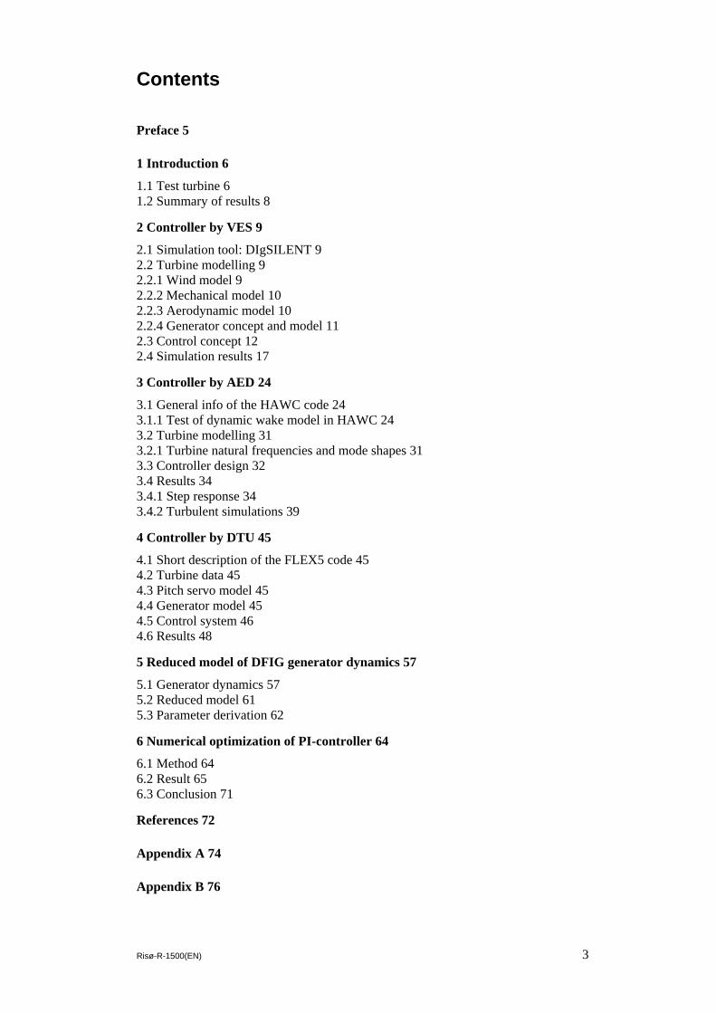
Contents

Preface 5

1 Introduction 6 1.1 Test turbine 6 1.2 Summary of results 8

2 Controller by VES 9 2.1 Simulation tool: DIgSILENT 9 2.2 Turbine modelling 9 2.2.1 Wind model 9 2.2.2 Mechanical model 10 2.2.3 Aerodynamic model 10 2.2.4 Generator concept and model 11 2.3 Control concept 12 2.4 Simulation results 17

3 Controller by AED 24 3.1 General info of the HAWC code 24 3.1.1 Test of dynamic wake model in HAWC 24 3.2 Turbine modelling 31 3.2.1 Turbine natural frequencies and mode shapes 31 3.3 Controller design 32 3.4 Results 34 3.4.1 Step response 34 3.4.2 Turbulent simulations 39

4 Controller by DTU 45 4.1 Short description of the FLEX5 code 45 4.2 Turbine data 45 4.3 Pitch servo model 45 4.4 Generator model 45 4.5 Control system 46 4.6 Results 48

5 Reduced model of DFIG generator dynamics 57 5.1 Generator dynamics 57 5.2 Reduced model 61 5.3 Parameter derivation 62

6 Numerical optimization of PI-controller 64 6.1 Method 64 6.2 Result 65 6.3 Conclusion 71

References 72

Appendix A 74

Appendix B 76

4 Risø-R-1500(EN)

Appendix C 80

Appendix D 81

Risø-R-1500(EN) 5

Preface The work presented in this report is part of the EFP project called “Aeroelastisk Integre-ret Vindmøllestyring” partly funded by the Danish Energy Authority under contract number 1363/02-0017.

The main objective of the project is to implement controller design of wind turbines in the general design process, in a similar way as is used for structural dynamics and aero-dynamics. Specific focus is on pitch-controlled turbines with variable speed. The poten-tial of future controllers will be identified and design limits will be mapped. As part of this, individual pitching of each blade based on load response input parameters will be treated, aiming at optimization of the operational state, reduction of loads and enhance-ment of stability characteristics.

The basis of the project is an existing traditional pitch controlled turbine with variable speed. General design tools for controller design using both linear and non-linear aeroe-lastic methods will be developed. These design tools will be verified using traditional methods, and optimum controller strategies will be developed. As part of this, the neces-sary changes in the structural and aerodynamic design will be identified, to obtain an optimum regulator.

The design of controller strategies will address the following main principles:

1. Optimization of power production with simultaneous load reduction of the main wind turbine components (gear box, tower, blades)

2. Adaptive control with respect to actual operational conditions.

Partners: IMM og MEK(DTU), VES.

Contact: Morten H. Hansen, [email protected], tel. +45 4677 5077

6 Risø-R-1500(EN)

1 Introduction This report deals with the design and tuning of the control system for the traditional pitch-regulated, variable speed wind turbine, where PI-regulators are used for regulating rotor speed and electrical power through the collective pitch angle and generator torque. Three different examples of controller designs for a specific test turbine are presented based on three different models of the aeroelastic and electrical systems.

The Wind Energy Systems research programme (VES) at Risø presents a controller de-sign with state-of-the-art electrical modelling and simplified aeroelastic modelling. The model and analysis are based on the simulation tool DIgSILENT.

The Aeroelastic Design research programme (AED) at Risø and Stig Øye from the De-partment of Mechanical Engineering at DTU present two controller designs with state-of-the-art aeroelastic modelling and simplified electrical modelling. The models and analyses are based on the simulation tools HAWC and Flex5, respectively.

The test turbine used for these investigations is described briefly in the following section. Sections 2, 3, and 4 contain the methods and results of the VES, AED, and DTU control-lers, respectively. Section 5 deals with the modelling of a Doubly-Fed Induction Genera-tor (DFIG), where also a reduced model is described which can be used for aeroelastic analyses in the lower frequency range. In Section 6, it is shown how to use a numerical optimization tool for improving the parameters of the PI-regulator in pitch control loop with respect to lower flapwise root bending loads. A summary of all results is given in the end of this introduction (Section 1.2).

1.1 Test turbine The test turbine for which a controller must be designed is described in this section. The data for the turbine is given in a HAWC format, see command file and input files in Ap-pendices A – D. The rated power of the turbine is 2 MW.

Figure 1 shows the aerodynamic power coefficient (Cp) surface computed with the aero-elastic stability tool HAWCStab based on the Blade Element Momentum method. Using HAWCStab, the optimal pitch angles and rotor speeds for maximum Cp have been com-puted based on this Cp–surface with a lower constrain on pitch angle and upper con-strains on rotor speed and power. The blue curve in Figure 1 represents the Cp for these optimal operational conditions, which are plotted in Figure 2. The lower constrain on the collective pitch angle was about 0.5 deg, and the upper constrains on rotor speed and power were 18.8 rpm (generator speed of 1600 rpm and gear ratio of 85) and 2 MW, re-spectively. Note that these operational conditions do not correct the power output for losses in the drive-train and generator, whereby the rated electrical power is assumed to be given by the maximal aerodynamic power of 2 MW.

Figure 3 shows the aerodynamic power and thrust for the test turbine with the opera-tional conditions shown in Figure 2. Rated power is reached at a wind speed of approxi-mately 12 m/s, where the rated rotor speed is reached around 10 m/s.

Finally, Figure 4 shows the natural frequencies of the first ten structural mode shapes of the test turbine computed with HAWCStab as function of the wind speed, where the ef-fects of pitch angle and rotor speed variations can be seen as changes in frequencies.

Risø-R-1500(EN) 7

Cp

-10-5

0 5

10 15

20

Pitch angle [deg]

0 0.05

0.1 0.15

0.2 0.25

0.3 0.35

0.4

Tip speed ratio [-]

0

0.1

0.2

0.3

0.4

0.5

Cp [-]

0

0.1

0.2

0.3

0.4

0.5

Cp [-]

Power optimal with pitch constrain

Cp [-]

Figure 1:Aerodynamic power coefficient surface with a curve representing the power coefficient at the operational conditions for optimal aerodynamic power with a lower constrain on pitch angle and upper constrains on rotor speed and power.

0

5

10

15

20

25

0 5 10 15 20 25 10

11

12

13

14

15

16

17

18

19

Col

lect

ive

pitc

h an

gle

[deg

]

Rot

or s

peed

[rpm

]

Wind Speed [m/s]

Pitch angleRotor speed

Figure 2: Operational conditions for op-timal aerodynamic power with constrains on pitch angle, rotor speed and power.

0

200

400

600

800

1000

1200

1400

1600

1800

2000

2200

0 5 10 15 20 25 50

100

150

200

250

300

Aer

odyn

amic

pow

er [k

W]

Thr

ust [

kN]

Wind Speed [m/s]

Aerodynamic powerThrust

Figure 3: Aerodynamic power and thrust for the test turbine with the operational conditions shown in Figure 2.

0

0.5

1

1.5

2

2.5

3

0 5 10 15 20 25

Nat

ural

freq

uenc

y [H

z]

Wind Speed [m/s]

1st lat. tower

1st long. tower

1st fixed-free shaft

1st flapwise BW

1st flapwise FW

1st sym. flap

1st edgewise BW

1st edgewise FW

2nd flapwise BW

2nd flapwise FW

Figure 4: Natural frequencies of the first ten structural turbine modes computed with HAWCStab as function of wind speed with the variation of pitch angle and rotor speed given in Figure 2.

8 Risø-R-1500(EN)

1.2 Summary of results The three different controller designs presented herein are similar and all based on PI-regulation of rotor speed and power through the collective blade pitch angle and genera-tor moment. The aeroelastic and electrical modelling used for the time-domain analysis of these controllers are however different, as mentioned above, which makes a directly quantitative comparison difficult. But there are some observations of similar and minor deviating behaviours should be mentioned:

• Very similar step responses in rotor speed, pitch angle, and power are seen for simulations of 1 m/s wind speed steps from 4 to 12 m/s and again from 12 to 20 m/s; also the tower top response computed by AED and DTU are very similar (cf. Figures 14, 31 and 42, and Figures 15, 33 and 43).

• All controllers show a peak in power for wind speed step-up over rated wind speed, which VES have shown can be almost removed by changing the parame-ters of the frequency converter (cf. Figure 16).

• Similar step responses in rotor speed, pitch angle, and power are seen for simu-lations of 2 m/s wind speed steps from 20 to 5 m/s computed by VES and DTU (cf. Figures 18 and 44), except that the VES controller shows a dip in power for all wind step-downs unless the integral term of speed controller is increased, re-quiring faster pitch activity.

• Responses of rotor speed, pitch angle, and power for different simulations with turbulent inflow are similar for all three controllers. Again, there seems to be an advantage of tuning the parameters of the frequency converter to obtain a more constant power output.

Note that the observed similarities in responses are mainly the result of similar tuning of the control parameters of the PI-regulator.

The dynamic modelling of the power controller is an important result for the inclusion of generator dynamics in the aeroelastic modelling of wind turbines. A reduced dynamic model of the relation between generator torque and generator speed variations is pre-sented, where the integral term of the inner PI-regulator of rotor current is removed be-cause the time constant is very small compared to the important aeroelastic frequencies. It is shown how the parameters of the transfer function for the remaining control system with the outer PI-regulator of power can be derived from the generator data sheet.

The main results of the numerical optimisation of the control parameters in the pitch PI-regulator performed in Chapter 6 are the following:

• Numerical optimization can be used to tune controller parameters, especially when the optimization is used as refinement of a qualified initial guess.

• The design model used to calculate the initial value parameters, as described in Chapter 3, could not be refined much in terms of performance related to the flapwise blade root moment (1-2 %) and tilt tower base moment (2-3 %).

• Numerical optimization of control parameters is not well suited for tuning from scratch. If the initial parameters are too far off track the simulation might not come through, or a not representative local maximum obtained.

The last problem could very well be related to the chosen optimization method, where more future work could be done.

Risø-R-1500(EN) 9

2 Controller by VES 2.1 Simulation tool: DIgSILENT DIgSILENT is a dedicated electrical power system simulation tool used for assessment of power quality and analysis of the dynamic interaction between wind turbines/wind farms with the grid.

DIgSILENT provides a comprehensive library of models for electrical components in power systems e.g.: generators, motors, controllers, power plants, dynamic loads and various passive network elements as e.g. lines, transformers, static loads and shunts. The program also provides a dynamic simulation language DSL which makes it possible for the users to create its own models library, as it is the case for the mechanical side of a wind turbine. Compared to HAWC and Flex5, the mechanical models implemented in DIgSILENT are relatively simpler, while the electrical models are very detailed.

2.2 Turbine modelling A simplified block scheme of the wind turbine model is shown in Figure 5. The basic block scheme of the wind turbine consists of a wind model, an aerodynamic model, a transmission system, generator model and a control block model.

2.2.1 Wind model The wind model used is described in detail in [1]. The main advantages of this wind model are the fast computation, reduced memory requirements and the ease of use, either for variable or constant speed models. This wind speed model is very suitable for simul-taneous simulation of a large number of wind turbines, making it possible to estimate efficiently the impact of a large wind farm on the power quality.

The structure of the wind model is shown in Figure 6. It provides an equivalent wind speed νeq to the aerodynamic model. The wind model includes two sub-models: a hub wind model and a rotor wind model.

The hub wind model models the fixed-point wind speed at hub height for each wind tur-bine. In this hub wind model, the park scale coherence can be taken into account in the case when a whole wind farm is modelled. The second is the rotor wind model, which contains an averaging of the fixed-point wind speed over the whole rotor, the rotational turbulence and the tower shadow model. The wind shear is not included in the rotor wind model, as it only has a small influence on the power fluctuations.

Windmodel

Control model

Aerodynamicmodel

DFIG model

bladeθ

rotorθrotorω genω

eqv rotT hssT

refP

gen

measPω

urotor

Mechanical model

irotor

Windmodel

Control model

Aerodynamicmodel

DFIG model

bladeθ

rotorθrotorω genω

eqv rotT hssT

refP

gen

measPω

urotor

Mechanical model

irotor

Figure 5: Scheme of wind turbine model.

10 Risø-R-1500(EN)

Hub wind modelFixed point wind speed

Wind turbineor

Wind farms(park scale wind model)

Rotor wind model

Averaged wind over rotor

Rotational turbulence

Tower shadow

hubuWind

Turbine

rotθ


Wind turbineor


Rotor wind model



Tower shadow



Tower shadow

hubuWind

Turbine

rotθ

eqυ


Wind turbineor


Rotor wind model



Tower shadow



Tower shadow

hubuhubuWind

Turbine

rotθ rotθ


Wind turbineor


Rotor wind model



Tower shadow



Tower shadow

hubuhubuWind

Turbine

rotθ rotθ

eqυ

Figure 6: Structure of the wind model.

Notice that the rotor position θrot is used in the wind model, and therefore this wind model can be used both variable speed and constant speed.

2.2.2 Mechanical model In the mechanical model, the emphasis is put only on those parts of the dynamic struc-ture of the wind turbine that contribute to the interaction with the grid. Therefore only the drive train is considered in the first place, because this part of the wind turbine has the most significant influence on the power fluctuations. The other parts of the wind tur-bine structure, e.g. tower and the flap bending modes, are neglected.

The mechanical model is shown in Figure 7. It is essentially a two mass model connected by a flexible low-speed shaft characterized by a stiffness k and a damping c. The high-speed shaft is assumed stiff. Moreover, an ideal gear with the ratio 1:ηgear is included.

The two masses correspond to the large turbine rotor inertia Jrot, representing the blades and hub, and to the small inertia Jgen representing the induction generator. The generator inertia is actually included in the generator model in DIgSILENT.

2.2.3 Aerodynamic model The aerodynamic model is based on tables with the aerodynamic power efficiency

),( λθpC or torque coefficient ),( λθqC , which depend on the pitch angle θ and on

the tip speed ratio λ. This is a quasistatic aerodynamic model which determines the out-put aerodynamic torque directly from the input wind speed according to:

2 31 ( , )2

rotrot p

rot rot

PT R u Cρ π θ λω ω

= = (1.1)

or

3 21 ( , )2rot qT R u Cρ π θ λ= (1.2)

Gearbox

Aerodynamic

Low speedshaft

High speedshaft Generator

1:η

Gearbox

Aerodynamic

Low speedshaft

High speedshaft

1:

Trot

Jrot

k

c

Tshaft

gear

θrot

Jgen

θgenGearbox

Aerodynamic

Low speedshaft

High speedshaft Generator

1:η

Gearbox

Aerodynamic

Low speedshaft

High speedshaft

1:

Trot

Jrot

k

c

Tshaft

gear

θrot

Jgen

θgen

Figure 7: Drive train model in DIgSILENT.

Risø-R-1500(EN) 11

The aerodynamic model, implemented in DIgSILENT, can also include a model for dy-namic stall [2,3]. The implemented model for dynamic stall is based on Øye’s dynamic stall model [4].

2.2.4 Generator concept and model A doubly-fed induction generator is basically a standards wound-rotor induction machine with the stator windings directly connected to the three-phase grid and with the rotor windings connected to a back-to-back partial scale frequency converter, which consists of two independent converters connected to a common dc-bus. These converters are il-lustrated in Figure 8, as rotor side converter and grid side converter.

The behaviour of the generator is governed by these converters and their controllers both in normal and fault conditions. The converters control the rotor voltage in magnitude and phase angle and are therefore used for active and reactive power control.

The doubly-fed induction generator (DFIG) model in DIgSILENT, illustrated in Figure 9, contains the usual induction machine model and the PWM rotor side converter in se-ries to the rotor impedance Zrot (DIgSILENT GmbH, 2002).

The line side converter is independent component in DIgSIlENT’s library and it can be added to the machine model to form the DFIG with back-to-back converter. The model equations of the doubly-fed machine can be derived from the normal induction machine equations by modifying the rotor-voltage equations:

1

( ) 1

syn ss ss s

n n

syn r rr rr r

n n

du R i j

dtd

u R i jdt

ψωψ

ω ωψω ω

ψω ω

= + +

−= + +

(1.3)

where u, i, and ψ are space vectors for the voltage, current and flux, respectively. ωsyn is the synchronous speed, ωr is the angular speed of the rotor, while ωn is the nominal elec-trical frequency of the network. Note that the equations are expressed in per unit system.

The dynamic model of the induction generator is completed by the mechanical equation:

WRIG Grid

ACDC AC

DC

Rotor sideconverter

Grid side converter

WRIG Grid

ACDC AC

DC

Rotor sideconverter

Grid side converter

Figure 8: Doubly-fed induction generator.

Figure 9: Doubly-fed induction generator model in DIgSILENT.

12 Risø-R-1500(EN)

r e mJ T Tω = − (1.4)

where J is generator inertia, Te is the electrical torque, Tm is the mechanical torque. This induction machine model of fifth order, based on Equations (1.3) and (1.4), is able to represent rotor and stator transients correctly. Applying the principle of neglecting stator transients to the doubly-fed induction machine model leads to the following third order model:

( ) 1

syns ss s

n

syn r rr rr r

n n

u R i j

du R i j

dt

ωψ

ωψω ω

ψω ω

= +

−= + +

(1.5)

The mechanical equation is the same as in case of the fifth order model.

2.3 Control concept Figure 10 sketches the control system of a variable speed DFIG turbine implemented in DIgSILENT. Two control levels using different bandwidths can be distinguished:

− Doubly-fed induction generator (DFIG) control level

− Wind turbine control level

The DFIG control, with a fast dynamic response, contains the electrical control of the power converters and of the doubly-fed induction generator. The DFIG control contains two controllers:

− Rotor side converter controller - controls independently the active and reac-tive power on the grid point M – see Figure 10.

Figure 10: Overall control system of variable speed wind turbine with doubly-fed induc-tion generator.

Risø-R-1500(EN) 13

− Grid side converter controller - controls the DC link voltage UDC and guaran-tees unity power factor in the rotor branch. The transmission of the reactive power from DFIG to the grid is thus only through the stator.

The wind turbine control, with slow dynamic response, provides reference signals both to the pitch system of the wind turbine and to the DFIG control level. It contains two controllers:

− Speed controller - has as task to control the generator speed at high wind speeds i.e. to change the pitch angle to prevent the generator speed becoming too. At low wind speeds, the pitch angle is kept constant to a optimal value.

− Maximum power tracking controller – generates the active power reference signal for the active power control loop, performed by the rotor side converter controller in DFIG control level. This reference signal is determined from the predefined characteristic P-ω look-up table, illustrated in Figure 11, based on filtered measured generator speed. This characteristic is based on aerodynamic data of the wind turbine’s rotor and its points correspond to the maximum aero-dynamic efficiency.

Both the speed controller and the maximum power-tracking controller are active in the power limitation strategy, while only maximum power tracking controller is active in the optimization power strategy. In the case of high wind speeds there is a cross coupling between these two controllers.

Figure 12 illustrates explicitly the speed controller, the maximum power tracking con-troller and the rotor side converter controller. The grid side converter controller is out of interest in the present study and therefore it is shown as a “black box”.

Figure 11: Power-omega characteristic used in the maximum power-tracking controller.

14 Risø-R-1500(EN)

Figure 12: Wind turbine control level.

In the rotor side converter control, there are two independent control braches, one for the active power control and the other for reactive power control. Each branch consists of 2 controllers in cascade. Only the active power control loops are relevant in the present study.

Notice that all these controllers, except maximum power tracking controller, are basi-cally PI controllers. Both the speed controller and the maximum power tracking has as input the filtered measured generator speed. The generator speed is measured and a low-pass filter is used to avoid that the free-free frequency in the transmission system is am-plified through the control system.

Speed controller implementation and design

The error between the filtered measured generator speed and the rated generator speed is thus sent to the PI speed controller. The output of this PI-controller is used as reference pitch signal refθ to the pitch system. To get a realistic response in the pitch angle con-

trol system, the servomechanism model accounts for a servo time constant Tservo and the limitation of both the pitch angle (0 to 30 deg) and its gradient (±10 deg/s). Thus the reference pitch angle refθ is compared to the actual pitch angle θ and then the error ∆θ

is corrected by the servomechanism.

A gain scheduling control of the pitch angle is implemented to compensate for the exist-ing non-linear aerodynamic characteristics.

Risø-R-1500(EN) 15

The total gain of the system in the speed control loop Ksystem, can be expressed as a pro-portional gain PIK in the PI controller times the aerodynamic sensitivity of the system

θddP

:

1

system PI basisdP dP dPK K Kd d dθ θ θ

−⎡ ⎤= = ⎢ ⎥⎣ ⎦

(1.6)

The aerodynamic sensitivity θd

dP of the system depends on the operating conditions (the

set-point power value, the wind speed or the pitch angle). The more sensitive the system is (larger pitch angles θ / higher wind speeds) the smaller the gain for the controller should be and vice versa.

The total gain of the system Ksystem is thus kept constant, by changing PIK in such a way

that it counteracts the variation of the aerodynamic sensitivity θd

dP by the reciprocal

sensitivity function1−

⎥⎦⎤

⎢⎣⎡

θddP

:

1

PI basisdPK Kdθ

−⎡ ⎤= ⎢ ⎥⎣ ⎦

(1.7)

where Kbasis is the constant designed proportional gain of the PI- controller. The varia-tions of the aerodynamic sensitivity with the pitch angle, implemented in DIgSILENT and Flex5 are illustrated in Figure 13. Note that an offset of 0.1 MW/deg is present be-tween these two curves. The reason is that in DIgSILENT the dynamic inflow is not taken into account.

Figure 13: Sensitivity function dP/dθ versus pitch angle θ.

16 Risø-R-1500(EN)

Assuming that the dynamic behaviour of the system can be approximated with a second order system behaviour, then the parameter design of the PI speed controller can be based on the transient response analysis for a second order system:

20

2 2 20 02

KI s D s K s s

ωξ ω ω

=+ + + +

(1.8)

where I, K and D denote the system inertia, stiffness and damping, respectively. Hence

the natural frequency and the damping ration can be expressed as: IK

=0ω and

00 22

1 ωω

ξK

DI

D== , respectively.

In the literature, two main parameterizations of the PI controller are applied:

PI controller - parameterization 1:

( )ip

Ky K us

= + (1.9)

where the proportional and integral gain can be expressed as (cf. Section 4):

1

0

0

and 230i

i p

gear

K KdPK KdN

ξθ ω

π

−Ω ⎡ ⎤= − ≅⎢ ⎥⎣ ⎦ (1.10)

In this PI controller parameterization form, the integral gain Ki is proportional to the stiffness K of the system, while the proportional gain Kp is proportional with the damp-ing of the system 0/2 ωξ KD = . Notice that when this parameterization is used, both

controller parameters contain gain scheduling, i.e. they vary with the reciprocal sensitiv-

ity function1−

⎥⎦⎤

⎢⎣⎡−

θddP

.

PI controller - parameterization 2:

1(1 )p

i

y K usT

= + (1.11)

where the integral time and the proportional gain are expressed as:

1

0

0 0

2 2 and 30p

i pi

gear

K K dPT KK dN

ξ ξω ω θ

π

−Ω ⎡ ⎤= = ≅ −⎢ ⎥⎣ ⎦ (1.12)

This parameterization of the PI controller is typically used in control systems. Notice that here only one parameter, i.e. the proportional gain Kp, has a proportional variation with

the reciprocal sensitivity function 1−

⎥⎦⎤

⎢⎣⎡−

θddP

, while the integral time Ti can be directly

determined based on design parameters (damping ration ξ and natural frequency ω0).

Risø-R-1500(EN) 17

The implementation in DIgSILENT of the PI controllers is using the parameterization 2. As design parameters in the controllers, there are used the damping ratio 66.0=ξ

and the natural frequency about 0.1 Hz (i.e. 6.00=ω ). Using the expressions (1.6) and

(1.12), the proportional gain Kbasis of the PI- controller can be expressed as:

0

0

230basis

gear

KKN

ξω

π

Ω= (1.13)

Based on design data (ξ and ω0) and on Equations (1.11) and (1.13), the parameters of

the PI speed controller (SC) become: 850=SCpK (normalized) and 2.2=SC

iT .

Active power control (rotor side converter controller)

The active power reference refconvgridP , signal, determined from the maximum power track-

ing look-up table, is further used in the active power control on the grid, performed by the rotor side converter controller.

The aim of the rotor side converter is to control independently the active and reactive power. As mentioned before, the attention, in this report, is mainly drawn to the active power control. The active power is controlled indirectly by controlling the impressed rotor current. As illustrated in Figure 12, the active power control, in DIgSILENT, con-tains two control loops in cascade: a slower (outer) power control loop and a fast (inner) rotor current control loop. The slower power control loop has thus as output the refer-ence rotor current signal, which is used further by the fast current control loop. The pa-rameters of the PI controllers in the rotor side converter are the following:

for the power controller (PC): 1.0=PCpK and 1.0=PC

iT

for the current controller (CC): 1=CCpK and 01.0=CC

iT

Notice that these two control loops existing in the rotor side converter controller and tak-ing care of the active power on the grid, are not implemented in HAWC and Flex5.

2.4 Simulation results To evaluate the performance of variable speed wind turbine controller implemented in power system simulation DIgSILENT a set of step response simulations with determinis-tic wind speed (no turbulence, no tower shadow) are performed. Typical quantities ver-sus of time are shown: wind speed in [m/s], pitch angle in [deg], generator speed in [rpm] and the generator power in [MW]. For comparison purpose, the scales of the fig-ures have been kept similar to those used in the FLEX5 simulations. Unless it is speci-fied, the simulations are performed using the parameters of the PI controllers, mentioned before.

In Figure 14, Figure 15 and Figure 16, the wind speed is stepped-up with 1m/s every each 20 s.

18 Risø-R-1500(EN)

Figure 14: Step in wind from 5 m/s to 12 m/s.

In the power optimization strategy (at low wind speeds less than 12 m/s), as illustrated in Figure 14, the speed controller is passive, keeping the pitch angle constant to the optimal value (i.e. zero for the considered wind turbine). Meanwhile, the power controller con-trols the active power to the active power reference signal provided by the maximum power tracking look-up table. The generator speed is thus continuously adapted to the wind speed, in such a way that it is extracted maximum power out of wind. Notice that the response time in the steps is bigger at lower wind speeds than at higher wind speeds.

At higher wind speeds than 12 m/s, illustrated in Figure 15, both the speed controller and the active power controller are active.

Risø-R-1500(EN) 19

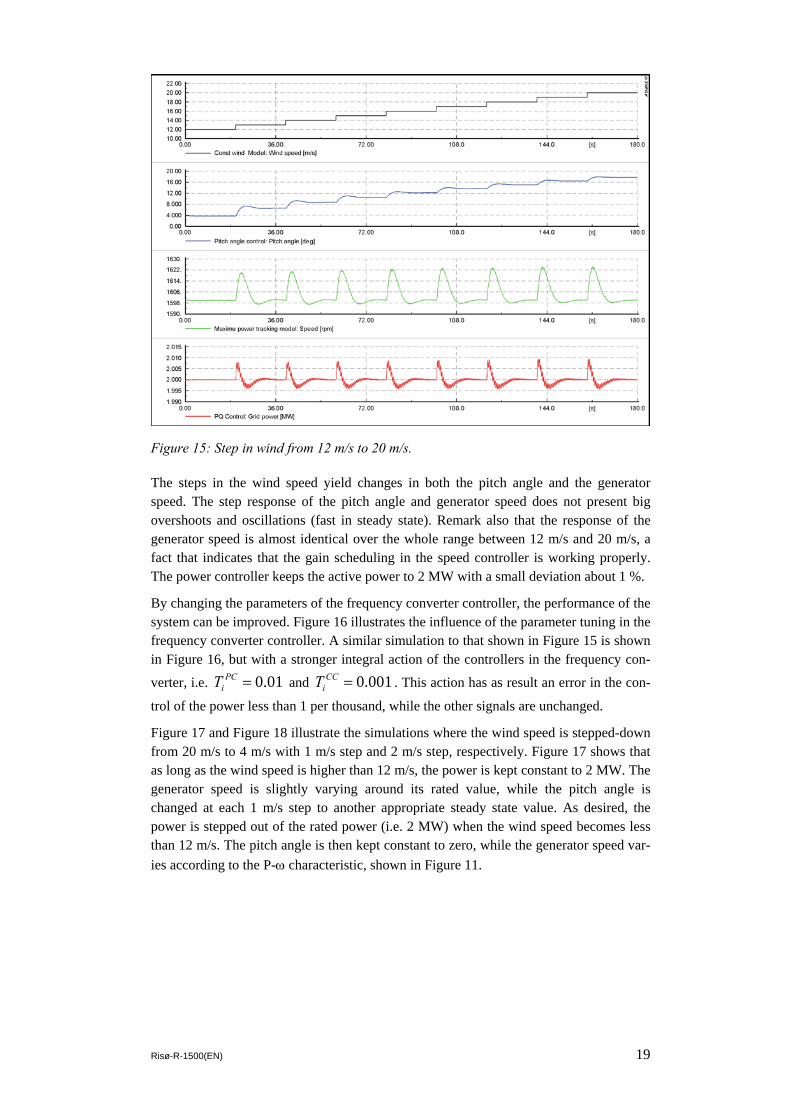
Figure 15: Step in wind from 12 m/s to 20 m/s.

The steps in the wind speed yield changes in both the pitch angle and the generator speed. The step response of the pitch angle and generator speed does not present big overshoots and oscillations (fast in steady state). Remark also that the response of the generator speed is almost identical over the whole range between 12 m/s and 20 m/s, a fact that indicates that the gain scheduling in the speed controller is working properly. The power controller keeps the active power to 2 MW with a small deviation about 1 %.

By changing the parameters of the frequency converter controller, the performance of the system can be improved. Figure 16 illustrates the influence of the parameter tuning in the frequency converter controller. A similar simulation to that shown in Figure 15 is shown in Figure 16, but with a stronger integral action of the controllers in the frequency con-

verter, i.e. 01.0=PCiT and 001.0=CC

iT . This action has as result an error in the con-

trol of the power less than 1 per thousand, while the other signals are unchanged.

Figure 17 and Figure 18 illustrate the simulations where the wind speed is stepped-down from 20 m/s to 4 m/s with 1 m/s step and 2 m/s step, respectively. Figure 17 shows that as long as the wind speed is higher than 12 m/s, the power is kept constant to 2 MW. The generator speed is slightly varying around its rated value, while the pitch angle is changed at each 1 m/s step to another appropriate steady state value. As desired, the power is stepped out of the rated power (i.e. 2 MW) when the wind speed becomes less than 12 m/s. The pitch angle is then kept constant to zero, while the generator speed var-ies according to the P-ω characteristic, shown in Figure 11.

20 Risø-R-1500(EN)

Figure 16: Influence of control parameters of the frequency converter.

Figure 17: 1m/s step-down in wind from 20 m/s to 5 m/s.

However, as it is illustrated in Figure 18, keeping the same control parameters (i.e.

2.2SCiT = ) also for the case when there is 2 m/s step in wind, reveals that the speed

controller is too lazy/slow. Due to the cross coupling between the controllers at high wind speeds, the power control is then not able to keep the power to the rated power. Figure 18 also illustrates the simulation when the integral action of the speed controller

is increased ( 0.5SCiT = ). A reduced integral time of the speed controller is correspond-

Risø-R-1500(EN) 21

ing to a lower damping ration or a higher natural frequency for the second order system. It means that to keep the power to the rated power, it is necessary to be able to force the generator speed to react faster to changes in the wind.

Note that such changing of the integral time of the speed controller yields to an increased rate of the pitch angle. This can off course imply both higher requirements to the pitch system and higher aerodynamic loads. As always, the choice of control parameters is and has to be a trade-off between different aspects. It seems that in the case of higher wind steps, as it is the case of gusts, the parameters designed through the transient response has to be slightly changed to be able to handle gusts in a satisfying way.

Figure 19 reflects the same aspects as Figure 18, but for the case of a turbulent wind with mean speed 20 m/s and turbulence 10 %. By making the speed controller faster, the power control manages to keep the power to the rated value, and to avoid thus the drops in the power.

Figure 20 illustrates the influence of better tuning of the parameters in the frequency converter controller. Notice that the frequency converter alone can improve the control of the power, without affecting the behaviour of the other signal, as i.e. the pitch angle and the generator speed.

Figure 18: 2 m/s step down in wind from 20 m/s to 5 m/s and influence of the speed con-troller.

22 Risø-R-1500(EN)

Figure 19: Turbulent wind. Influence of integral time of the speed controller.

Figure 20: Turbulent wind. Influence of frequency converter.

Figure 21 illustrates a simulation of variable speed wind turbine with turbulent wind, where the mean is 8 m/s and the turbulence intensity of 10 %.

The generator speed is tracking the slow variation in the wind speed. As expected for this wind speed range, the pitch angle is passive, being kept constant to its optimal value (i.e. zero for the considered wind turbine). The active power delivered to the grid does reflect

Risø-R-1500(EN) 23

the variation in the wind speed. Notice that the fast oscillations in the wind speed are completely filtered out from the electrical power.

Figure 22 illustrates the simulation with turbulent wind, where the mean speed is 12 m/s and the turbulence intensity of 10 %. The power is kept to the rated power as long as the energy in the wind permits that.

Figure 21: 8 m/s turbulent wind (turbulence 10 %).

Figure 22: 12 m/s turbulent wind (turbulence 10 %).

24 Risø-R-1500(EN)

3 Controller by AED 3.1 General info of the HAWC code HAWC [5] is a computer program with the purpose of predicting load response for a horizontal axis two and three bladed wind turbine in time domain including all aspects that might be important for the dynamic loads. The program consists of several sub-packages, each dealing with a specific part of the turbine and the surroundings.

The core of the program is the structural model, which is a finite element model based on Timoshenko beam elements. The turbine is divided into three substructures: Tower, na-celle and rotor blades. Each substructure has its own coordinate system allowing for large rotation of the substructures. There are six degrees of freedom (DOFs) for each element node, i.e., for at typical wind turbine the total number of DOFs is approx. 250.

The aerodynamic model is based on a modified Blade Element Momentum (BEM) model. This model has through the years of development evolved from a static frozen wake method to a dynamic wake formulation including corrections for yawed flow. The local aerodynamic load is calculated at the blade sections using 2D lift, drag and moment profile coefficients. Unsteady aerodynamic effects are modelled by a Beddoes-Leishman type dynamic stall model.

The wind field turbulence model used for load simulations is the Mann model [6]. This model is a full 3D turbulence field with correlation between the turbulence in the three directions. The turbulence field is a vector field in space; a so-called frozen snapshot of the turbulent eddies in the wind. This turbulence is transported through the wind turbine rotor with the speed of the mean wind speed. It is also possible to use the wind format from a FLEX wind generator, but this feature has not been used in the present simula-tions.

The HAWC model is equipped with interface for control systems through a Dynamic Link Library (DLL) format [7]. This interface enables control of the turbine pitch angles and generator torque from a control program outside the HAWC core.

The generator model used for these simulations is based on a simple assumption that the generator torque can be controlled as desired by the regulator, but with a small phase delay corresponding to a 1st order filter with a time constant of 0.1 s.

The pitch servo is implemented as a 1st order filter with a time constant of 0.2 s and a max. allowable speed of 20 deg/s. Some extra features regarding offshore foundations and wave interactions are also sub-packages in the program, but not used for simulations related to this report.

3.1.1 Test of dynamic wake model in HAWC To evaluate the dynamic wake model that is implemented in HAWC a few simulation without turbulence has been performed. The controller for these simulations are a bit special since it is implemented as an asynchronous generator providing an almost con-stant rotor speed, and a pitch regulator keeping the power at nominal by adjusting the pitch angle. After a certain time the pitch angle is increased in one step with 0.5 deg and back again a little bit later. The dynamic load changes have been plotted in Figure 23 to Figure 28.

Risø-R-1500(EN) 25

Figure 23: Simulation at 5 m/s. Step change in pitch angle at constant rotor speed. The induction changes slowly from one level to another causing momentary load changes that flatten off when the induction reaches a new equilibrium. From top: Rotational speed, pitch angle (opposite sign than normal convention), electrical power, blade flap root moment, induced wind speed longitudinal, induced wind speed tangential.

26 Risø-R-1500(EN)


Risø-R-1500(EN) 27


28 Risø-R-1500(EN)


Risø-R-1500(EN) 29


30 Risø-R-1500(EN)


Risø-R-1500(EN) 31

3.2 Turbine modelling 3.2.1 Turbine natural frequencies and mode shapes The turbine has been modelled based on data delivered by Risø. Natural frequencies and corresponding damping levels are shown in Figure 29 and Table 1. A vibration mode of utmost importance for control design is the free-free vibration in the drive train, which is not shown in the Figures since these calculations are performed with a fixed generator (corresponding to a clamped brake situation). This vibration mode is primarily the rotor and generator vibrating in counter phase. A simplified expression to calculate this fre-quency is:

2

2

1 11

1 122

r gfree free

edge r shaft

I n IF

F I Kπ

π

−

+=

+

where Ir is the rotational inertia of the rotor, n is the gear exchange ratio, Ig is the rota-tional inertia of the generator at the high speed shaft, Fedge is the 1st edgewise blade bend-ing frequency and Kshaft is the torsional stiffness of the drive train system. For the current turbine this frequency is calculated to 1.67 Hz (corresponding to 5.3P).

Turbine mode Frequency [Hz] Damping [log. decr. %]

1st tower long. bending 0.34 2.94

1st lateral tower bending 0.35 2.93

1st shaft torsion 0.61 3.58

1st yaw 0.94 2.47

1st tilt 1.01 2.74

1st symmetric flap 1.21 3.53

1st horizontal edge 1.68 3.03

1st vertical edge 1.77 3.36

2nd yaw 2.39 6.51

2nd tilt 2.47 8.18

Table 1: Frequency and corresponding damping at standstill calculated with HAWCStab.

32 Risø-R-1500(EN)

Figure 29: Mode shapes at stand still for 2 MW test turbine calculated with HAWC. See list of frequencies and corresponding damping levels in Table 1.

3.3 Controller design The turbine controller is basically a PI-regulator that adjusts the pitch angles and genera-tor on basis of measured rotational speed. The controller diagram can be seen in Figure 30 In this Figure different parts of the regulation can be seen. In basic the regulator con-sist of a power controller and a pitch controller. The power controller is adjusting the reference power of the generator based on a table look up (2) with input of the rotor speed. This table has been created on basis on quasi-static power calculations. In this

Risø-R-1500(EN) 33

table the overall characteristics of the turbine control regarding variable speed, close to rated power operation and power limitation operation are given.

In the power regulation it is important to avoid too much input of especially the free-free drive train vibration. If not taken into consideration, this vibration could very well be amplified through the power control creating very high torque oscillations.

Therefore a special band stop filter (1) has been applied to filter out this vibration fre-quency. For the current turbine the filter is implemented as a 2nd order Butterworth filter with center frequency at the free-free eigenfrequency.

To limit the aerodynamic power to the turbine a PI-regulator (3) is applied that adjusts the reference pitch angle based on the error between rotational speed and rated speed. The PI-regulator has a minimum setting of zero deg, which makes the turbine operate with zero pitch angles at low wind speeds. The proportional and integral constants Kp and Ki are set to respectively 1.33 and 0.58, which corresponds to a frequency of 0.1 Hz and a damping ratio of 0.6.

A special gain scheduling (5) to adjust for increased effect of pitch variations at high wind speed compared to lower speeds is applied. This gain scheduling handles the linear increasing effect of dP/d θ with increasing wind speed and pitch angle. This gain func-tion is implemented following the expression gain(θ) = 1/(1+θ /KK), where the value KK is the pitch angle where the gain function shall be 0.5 (cf. Section 4).

To increase the gain when large rotor speed error occurs another gain function (4) is ap-plied to the PI-regulator. This gain function is simply 1.0 when the rotor speed is within 10 % of rated speed and 2.0 when the error exceeds 10 %. This very simple gain function seems to limit large variations of the rotational speed at high wind speed.

The pitch servo is modelled as a 1st order system with a time constant of 0.2 s. The maximum speed of the pitch movement is set to 20 deg/s.

The generator is modelled as a 1st order system with a time constant of 0.1 s, which means that the reference torque demand from the regulator has a little phase shift before executed.

Figure 30: Control diagram of regulator. Input is measured rotational speed and output is reference electrical power to generator and reference collective pitch angle to pitch servo.

34 Risø-R-1500(EN)

A drive train filter has been included in the generator model to decrease response at the free-free drive train frequency. This filter makes sure that any torque demand at the free-free frequency is in counter phase before entering the structural model.

3.4 Results 3.4.1 Step response To evaluate the behaviour of the controller a step response simulation has been per-formed. The wind speed is increased for every 20 s with 1 m/s. There are no turbulence, tower shadow or wind shear. Only the tilt angle of 6 deg contributes to varying aerody-namic during a rotor revolution.

In Figure 31 to Figure 34 the results of the step simulation are shown. At low wind speed the controller operates with constant pitch angle of zero degree and varying rotational speed. It takes quite some time (app. 30 s.) for the rotational speed to change from level to another. The result of this is that in a turbulent situation the rotor speed will never be optimal. Since the consequence of a too low rotor speed is a much low power output than if the rotor speed was a little too high it might be a good idea to change the rotor power-speed characteristic in the controller to a bit lower values of demanded power than the optimal values calculated from quasi static analysis. This will make the rotor speed a little higher than the optimal value and the average power output in a turbulent situation will increase a little.

At high wind speeds the rotational speed vary around the rated speed. The response of the rotational speed is almost identical whether the wind speed is stepping from 12 m/s or 20 m/s which indicates that the gain scheduling in the controller is good. The response of the tower in the longitudinal is highly damped which is not the case for the lateral di-rection. The loads are however largest in the longitudinal direction. The cyclic loads on the rotor originating from the 6 deg tilt angle can mainly be seen in the flapwise bending moment, the rotational bending at hub, and the tower top tilt moment. The effects of these increase with wind speed. For the yaw moment there is a sign change in the mo-ment direction close to rated power. At low wind speed the yaw moment is very small though negative where the yaw moment increased as the pitch angles increases. The rea-son for the significant level of yaw moment at high wind speed is the lift forces on the pitched blades have a moment arm around the tower centerline, which increases with pitch angle.

Risø-R-1500(EN) 35

Figure 31: Step response with steps from 5 m/s to 11 m/s. From top: wind speed, rota-tional speed rotor, electrical power, pitch angle (opposite sign than normal convention), tower top deflection lateral, tower top deflection longitudinal.

36 Risø-R-1500(EN)

Figure 32: Step response with steps from 5 m/s to 11 m/s. From top: Flap root moment, rot. bending moment at hub, driving torque at hub, tilt moment at tower top, yaw moment at tower top, angle of attack in 3/4 radius.

Risø-R-1500(EN) 37

Figure 33: Step response with steps from 11 m/s to 25 m/s. From top: wind speed, rota-tional speed rotor, electrical power, pitch angle (opposite sign than normal convention), tower top deflection lateral, tower top deflection longitudinal.

38 Risø-R-1500(EN)

Figure 34: Step response with steps from 11 m/s to 25 m/s. From top: Flap root moment, rot. bending moment at hub, driving torque at hub, tilt moment at tower top, yaw moment at tower top, angle of attack in 3/4 radius.

Risø-R-1500(EN) 39

3.4.2 Turbulent simulations

Figure 35: Simulation at 5 m/s at 10 % turb. intensity. From top: wind speed, rotational speed rotor, electrical power, pitch angle (opposite sign than normal convention), tower top deflection lateral, tower top deflection longitudinal.

40 Risø-R-1500(EN)

Figure 36: Simulation at 5 m/s at 10 % turb. intensity. From top: Flap root moment, rot. bending moment at hub, driving torque at hub, tilt moment at tower top, yaw moment at tower top, angle of attack in 3/4 radius.

Risø-R-1500(EN) 41

Figure 37: Simulation at 12 m/s at 10 % turb. intensity. From top: wind speed, rota-tional speed rotor, electrical power, pitch angle (opposite sign than normal convention), tower top deflection lateral, tower top deflection longitudinal.

42 Risø-R-1500(EN)


Risø-R-1500(EN) 43

Figure 39: Simulation at 22 m/s at 10 % turb. intensity. From top: wind speed, rota-tional speed rotor, electrical power, pitch angle (opposite sign than normal convention), tower top deflection lateral, tower top deflection longitudinal.

44 Risø-R-1500(EN)


Risø-R-1500(EN) 45

4 Controller by DTU 4.1 Short description of the FLEX5 code FLEX5 is a computer program designed to model the dynamic behaviour of horizontal axis wind turbines operating in specified wind conditions including simulated turbulent wind. The program operates in the time domain and produces time-series of simulated loads and deflections.

The structural deflections of the turbine are modelled using relatively few but carefully selected degrees of freedom using shape functions for the deflections of the tower and the blades while using stiff bodies connected by flexible hinges to model the nacelle, rotor shaft and hub.

The aerodynamic loads on the blades are calculated by the normal Blade-Element-Momentum method modified to include the dynamics of the induced velocities of the wake. This dynamic wake model is important for a realistic prediction of the response due to pitch angle changes and hence for the design of the control system of a pitch con-trolled wind turbine.

The properties of the pitch servo, the generator and the control system are modelled in separate modules of the program and can be selected from a library of standard models or can be programmed by the user. These models will be described in more detail below.

4.2 Turbine data The structural and aerodynamic data for the generic 2 MW variable speed, pitch con-trolled wind turbine have been provided by Risø in the format designed for the HAWC code, see Appendices A to D.

While the airfoil data can be used directly, the structural data have been used to produce an equivalent FLEX5 input file with properties that result in a turbine model with the same primary natural frequencies as the HAWC model. These frequencies were provided by Risø in addition to the HAWC data files.

4.3 Pitch servo model The pitch servo is modelled to be following a setpoint angle signal from the control sys-tem with a simple 2.order response with specified resonance frequency and damping. This will simulate a hydraulic servo system with position feedback with sufficient accu-racy for the present purpose. The frequency and damping ratio have been chosen as 0.8 Hz and 0.8 (relative to critical). These values produce a good fit to the actual pitch servo response of the old 2 MW Tjæreborg turbine.

4.4 Generator model The FLEX5 generator model is used to prescribe the generator air gap torque while the inertia of the generator rotor is part of the turbine structural model. Any losses (mechani-cal and electrical) are simulated by adding an equivalent torque to the simulated airgap torque.

The generator model used for this case is a simplified model of a variable speed genera-tor where the electrical output is assumed to be controlled by some unspecified generator controller in direct response to a power setpoint specified by the wind turbine control system. No attempt has been made to simulate the actual electrical properties of the gen-

46 Risø-R-1500(EN)

erator or the grid connection. The generator torque is simply calculated as the setpoint power + losses divided by the generator rotational speed. However, to avoid instability of the free-free torsional mode of the rotor shaft when operating at constant power, the rotational speed signal is put through a 2.order low pass filter before the division is car-ried out. The filter frequency is chosen as 0.8 Hz with a damping ratio of 0.7, which at the free-free shaft frequency of 1.65 Hz provides sufficient attenuation and phase lag to avoid the instability.

Also, the setpoint power signal is put through a 1.order filter with a time constant of 0.5 s. This is done to avoid too abrupt power changes due to steps in the power setpoint.

The combined losses (mechanical and electrical) are assumed to be 2%, 4% and 8% at a load of 0%, 50% and 100% respectively (parabolic interpolation).

4.5 Control system The FLEX5 control system model for the variable speed, variable pitch turbine simulates two simple controllers: a generator power versus rotor speed controller and a PI-pitch angle control of the rotor speed. The two controllers are designed to work independently in the below rated and the above rated wind speed range respectively.

The generator power controller specifies the power setpoint for the generator as a tabulated function of the generator speed. The speed signal input is the lowpass-filtered RPM-signal used in the generator model. The tabulated power vs. generator speed func-tion for the 2 MW turbine is shown in Figure 41.

The data for the lower part of the curve up to 800 kW / 1500 RPM has been chosen in such a way that the generator torque controls the rotor speed to be approximately propor-tional to the wind speed up to about 8.5 m/s with a tip speed ratio of 8.7 (optimum). Above 9 m/s the rotor speed would become too large if the constant tip speed ratio were continued. Therefore a much steeper, linear slope is introduced up to the rated power of 2 MW at 1580 RPM. This part will control the rotor speed for wind speeds between 8.5 and 12 m/s (rated). The control mode corresponds to the operation of a constant speed turbine with a large slip asynchronous generator. If the turbine accelerates to above 1580 RPM due to wind speed above 12 m/s (rated) the generator power is kept at a constant 2 MW in which case there is no longer any control of the RPM from the generator torque.

Figure 41: Generator power setpoint as function af generator speed.

Risø-R-1500(EN) 47

This is where the pitch control takes over.

The pitch angle controller is a simple PI-controller with the generator speed (low pas filtered) as input and the pitch servo set-point as output. The reference speed of the con-troller is 1600 RPM, which is sufficiently above the speed for maximum generator power to allow for fluctuations around the reference (target) speed without interference from changes in the generator power. This makes the design of the PI-controller very simple.

If we assume that the turbine is stiff so that shaft rotation as the only degree of freedom it is possible to derive the following 2nd order differential equation for the shaft rotation angle when the PI-control is active and the generator operates at constant power:

0I D Kϕ ϕ ϕ+ + = (3.1)

where 0ϕ = Ω − Ω is angular velocity of the rotor speed difference between actual and

reference speed. The parameters of the 2nd order differential equation are

2

02

0 0

0

1 30

1 30

rotor gear generator

P gear

I gear

I I N I

PdPD K NddPK K Nd

θ π

θ π

= +

⎛ ⎞= − −⎜ ⎟Ω Ω⎝ ⎠

⎛ ⎞= −⎜ ⎟Ω ⎝ ⎠

(3.2)

Within the limits of the simplifying assumptions it can be seen that the PI-control system will have a 2nd order response with the following resonance frequency and damping ra-tio:

00

and 2 2

K D DI I KI

ω ξω

= = = (3.3)

Experience shows that a satisfactory response is obtained by choosing the frequency and damping as follows:

0 0.6 rad/s and 0.6 0.7ω ξ≅ ≅ − (3.4)

The corresponding values of the constants KP and KI of the PI-controller can now be calculated when the pitch sensitivity dP/dθ is known. This quantity must be calculated from the aerodynamic properties of the rotor. For a number of wind speeds above rated ordinary static BEM-calculations are performed to determine the pitch angle that pro-duces the rated mechanical power at each wind speed at the reference RPM. At each of these operational situations the derivative dP/dθ is calculated by doing two new calcula-tions with small changes of the pitch angle to each side but still using the same induced velocities as the central calculation (frozen wake assumption).

The calculated pitch sensitivity will show a large variation with wind speed (numerically increasing with increasing wind) so constant values of KP and KI will not give the de-sired result because of the change in total gain. However, if we plot the pitch sensitivity as a function of the pitch angle, we will find a nearly linear relation. This implies that a gain correction factor GK(θ) = 1/(1+θ /KK) multiplied with both KP and KI will solve the problem and produce nearly constant gain over the range of relevant wind speeds. The constants KP and KI are now calculated using the value of dP/dθ corresponding to 0 deg. pitch while the parameter KK is determined as the pitch angle where dP/dθ has

48 Risø-R-1500(EN)

increased by a factor of 2. This type of gain correction factor has been used with success for both the old Nibe B and Tjæreborg turbines.

Regarding the present 2 MW turbine the following values have been found according to the method above. These values are used in the following FLEX5 simulations.

KP = 0.14 deg/RPM KI = 0.06 deg/s/RPM KK = 6.2 deg

The pitch setpoint provided by the PI-controller is the sum of the proportional term and the integral term. The values of the integral term alone and the total sum must be limited to a certain minimum angle to prevent the integral term from saturating and to prevent the pitch angle from hitting the physical stops during operation in wind speeds below rated. The FLEX5 implementation allows this minimum angle to be prescribed as a func-tion of the wind speed at the hub averaged over time by a 1.order filter with a specified time constant. For the test examples below the time constant is only 6 s. It would nor-mally be 30 to 60 s. This minimum angle will be the angle at which the turbine operates at winds below rated. The minimum angel is specified as a tabulated function of the wind speed. Below 10 m/s the angle is 0 deg. From 10 to 12 m/s the angle increases to +1 deg. and further to +6 deg. at 16 m/s and above. The idea behind this is to limit the maximum blade load and prevent potential stalling of the blades when operating in turbulence around rated wind speed.

One further feature has been implemented: When the turbine operates in turbulence above rated wind speed the rotor speed will vary somewhat around the reference RPM and might sometimes even deviate below the RPM for max generator power. This will result in a short, but possibly deep reduction of the generator power even if there is suffi-cient wind available to produce max. power continuously. This is avoided to a large de-gree by including a conditional statement for the power controller: if the pitch angle is more than 1 deg. above the specified minimum angle at the current wind speed the power setpoint should be kept at max. power independent of the instantaneous RPM. The result is a much improved power quality (fewer dips) at the expense of some short term over-loading of the generator and gearbox (larger torque due to lower RPM).

Finally, please note that the inevitable sampling and processing delays are not simulated. This could lead to somewhat optimistic results regarding the controller performance.

4.6 Results Eight test examples have been simulated with the FLEX5 code to illustrate the perform-ance of the control system. The results are shown as time series plot of selected “sen-sors” in the figures on the following pages. The two time-series plotted at the bottom of each figure show the tower top deflections in the longitudinal (wind) direction (L) and in the transverse direction (T)

The first 3 simulations show the response to idealised steps in the wind input with no turbulence. The following five figures show the results from simulations with turbulent wind at 5 different mean wind speeds with a turbulence intensity of 10%.

Even though the control system is only a first try with no detailed optimisation done, the results show a very well behaved response.

Risø-R-1500(EN) 49

Figure 42: Step responses for wind speed steps from 4 – 12 m/s.

50 Risø-R-1500(EN)


Risø-R-1500(EN) 51


52 Risø-R-1500(EN)

Figure 45: Responses at mean wind speed of 8 m/s and turbulence intensity of 10 %.

Risø-R-1500(EN) 53


54 Risø-R-1500(EN)


Risø-R-1500(EN) 55


56 Risø-R-1500(EN)


Risø-R-1500(EN) 57

5 Reduced model of DFIG generator dynamics This chapter describes the dynamics of the doubly-fed induction generator, derives a strongly reduced model of the generator including converter and control, and finally de-rives the parameters of the reduced model based on generator data sheet information, and compares the parameters to estimates based on simulations with the detailed DIgSILENT model described in Chapter 2.

The dynamics included in the reduced model represents the power controller of the gen-erator, whereas the generator itself including the rotor current control is modelled in steady state. This is possible because the response from rotor current reference as input to torque as output is very fast. The rotor speed is assumed constant in the first place, but it is straightforward to extend the model with the dynamics due to the generator inertia, because the generator torque is output of the model.

The idea is to provide a simple generator model, which is useful in design models for wind turbine controllers. The model can also be applied in aeroelastic models of wind turbines.

5.1 Generator dynamics The generator dynamics dealt with in this chapter includes the DFIG control level shown in Figure 12 in addition to the generator. Only the active power dynamics are dealt with here, because reactive power only has marginal influence on the mechanical part.

Figure 50 shows the power control of the doubly fed induction generator with a few ad-ditions to Figure 12. Some of the variables are in p.u. values, which is often used in elec-trical systems. The p.u. value is defined as the ratio between the physical value and a certain base, which is often a rated value. Thus, it is of course essential to use the correct base.

As mentioned in Chapter 2, the controller is a cascade of two PI controllers. The first PI-controller (the power controller) is the slowest, with an integration time TiP = 10 ms in the DIgSILENT model. It controls the power Pgrid to the reference value Pgrid

ref set by the wind turbine controller. The integration time can be changed like the rest of the control-ler dynamics, because this part of the model is completely open to the DIgSILENT user, but the PI controller with TiP = 10 ms has shown to give stable response.

The output of the power controller is the reference of the q component iqref of the rotor

current, which is given in p.u. in the stator flux coordinate system. The stator flux coor-

PIref

gridPrefqi

PImqP

Genmeasqimeas

gridP

tpgenω

Gridrs PP ,

Mechanicalsystem

p.u.conv.

mecT genΩ

Figure 50. Block diagram for power control of doubly-fed induction generator.

58 Risø-R-1500(EN)

dinate system is defined with d-axis collinear with the stator flux linkage, which rotates synchronously with the power system frequency f0=50 Hz.

The reason to chose the stator flux coordinate system is that the cyclic (sinusoidal) varia-tions of the electric variables (voltages, currents, flux) are removed. Also, in the stator flux coordinate system, which is very close to the stator voltage coordinate system, a change of the current in the q direction mainly results in changed active power, while a change in the current in the d-direction mainly causes changed reactive power.

The second PI-controller is the rotor current controller. It controls the rotor current iqmeas

to the reference value iqref with an integration time Tii = 1 ms. The output of the rotor

current controller is the modulation factor Pmq, given also in the stator flux coordinate system. The modulation factors Pmd and Pmq determine the rotor side converter voltage, and they are defined as the fraction of the dc voltage Udc (see Figure 10), e.g. Uq = Pmq Udc.

Summarising the control cascade, a power reference is set by the first controller. The output of that controller is a reference value of the generator rotor current. The second controller has the rotor current as input and the voltage for the rotor side converter as output.

The generator in Figure 50 is shown as a black box. Note that the input to the build-in DIgSILENT generator model is the turbine power pt. The generator inertia J is also built into the generator model according to (2.4). Thus, the used output form the generator model is the rotor speed, and not the generator torque.

A “p.u. conv” block is given between the generator block and the mechanical system model. The purpose of the “p.u. conv” block is to convert the physical unit values in the mechanical model to the p.u. values in the build-in generator model, and to be able to keep the mechanical torque Tmec constant rather than the mechanical power pt.

Finally a grid block is shown in Figure 50 to indicate the feedback from the generator to the measured power. The generator produces stator power Ps as well as rotor power Pr, and the total grid power Pgrid is measured on the other side of the transformer (see Figure 10).

Figure 51 shows the dynamic response to a stepwise change in power reference, simu-lated with the DIgSILENT model. The aerodynamic torque is kept constant in the simu-lation. The response is simulated with the original integration time TiP = 10 ms and with a ten times slower integration time TiP = 100 ms, to illustrate that the dynamics of the step response is mainly due to this integration time.

Risø-R-1500(EN) 59

Figure 52 shows the dynamic response to a stepwise change in the rotor current refer-ence. In this case, the turbine power pt is kept constant. It is seen that the power response to the change in rotor current reference is very fast.

Pref

0 0.05 0.1 0.15 0.2 0.25 0.3 0.35 0.4 0.45 0.5

1.9

1.92

1.94

1.96

1.98

Time [s]

Pow

er [M

W]

0 0.05 0.1 0.15 0.2 0.25 0.3 0.35 0.4 0.45 0.50.83

0.835

0.84

0.845

0.85

0.855

0.86

0.865

0.87

0.875

Time [s]

Rot

or c

urre

nt [p

u]

ms10=iPT

ms100=iPT

),( ms 100 rfqrefrfqiP iiT =

),( ms 10 rfqrefrfqiP iiT =

Figure 51. Dynamic response to step in power reference.

0.200.160.120.080.040.00 [s]

0.45

0.43

0.41

0.39

0.37

0.35

0.200.160.120.080.040.00 [s]

0.95

0.90

0.85

0.80

0.75

0.200.160.120.080.040.00 [s]

0.05

0.03

0.01

-0.010

-0.030

-0.050

0.200.160.120.080.040.00 [s]

0.45

0.43

0.41

0.39

0.37

0.35D

IgSI

LEN

T

i qr ef

[pu ]

i qmea

s[p

u]P m

q[p

u ]P g

ridm

eas

[MW

]

Figure 52. Dynamic response to step in rotor current reference.

60 Risø-R-1500(EN)

For aeroelastic models, it is of interest how the generator torque responds to changes in generator speed. For frequencies around 1 Hz and below, the directly connected squirrel cage induction generator responds approximately to the well-known steady-state torque characteristics, which increases the torque when the speed is increased, and consequently damps the free-free oscillations of the generator inertia against the turbine rotor inertia.

Since it is not possible to change the speed as input to the DIgSILENT model, the me-chanical torque is changed sinusoidal instead, and the torque is plotted vs. the speed as shown in Figure 53.

Finally, the response to step changes in the modulation factor has been simulated with the detailed DIgSILENT model. The simulation results are shown in Figure 54. In this case, the inertia is multiplied by 1000 in the simulations to reduce the influence of speed changes and focus on the electrical response.

1.08131.06941.05761.04571.03391.0221 [-]

0.700

0.699

0.697

0.695

0.694

0.692

[p.u.]

G: Speed/Electrical Torque in p.u.G: Speed/Electrical Torque in p.u.

DIg

SILE

NT

1 Hz5 Hz

Elec

tric a

l tor

que

[pu]

Generator speed [pu]

1 Hz

5 Hz

Tii = 0.01 msecTii = 0.01 msec

Tii = 0.001 msecTii = 0.001 msec

Figure 53. Generator torque vs. speed for 1 Hz and 5 Hz variations in mechanical torque.

1.000.800.600.400.200.00 [s]

0.50

0.45

0.40

0.35

0.30

0.25

1.000.800.600.400.200.00 [s]

1.000

0.90

0.80

0.70

0.60

0.50

1.000.800.600.400.200.00 [s]

0.35

0.30

0.25

0.20

0.15

0.10

1.000.800.600.400.200.00 [s]

0.0045

0.0040

0.0035

0.0030

0.0025

0.0020

DIg

SILE

NT

i dmea

s[p

u ]i qm

eas

[pu]

P mq

[pu ]

P gri

dmea

s[M

W]

Figure 54. Dynamic response to step in modulation factor.

Risø-R-1500(EN) 61

There is a coupling between id and uq, which is very weak in Figure 54. Lindholm [9] has shown that this coupling is proportional to the slip. Lindholm also suggested an algo-rithm to eliminate the cross coupling, but this has not been implemented in the DIgSI-LENT model. To minimise the coupling in the example, a working point with a very low slip (0.05%) has been selected for the simulations in Figure 54.

According to Lindholms results, when the slip is zero, the dynamic equation is of the rotor in stator flux dq-coordinates is

dtdi

LiRu qrqrq σ+= (5.1)

where σ is the leakage factor

rs

m

LLL 2

1−=σ (5.2)

With the parameters for the present generator, (5.1) is a first order system with the tran-sient rotor time constant

ms 110==r

rr R

Lστ (5.3)

The transient rotor time constant can be seen in Figure 54 in the response of iq and the power immediately after the step in Pmq. It is observed that the power and torque re-sponse to a step in the rotor voltage (implemented as a step in the modulation factor) is much slower than the response to a step in the rotor current reference. Thus, the current controller speeds up the response considerably. As a result of this speed up, the rotor voltage has to respond with a transient, which is also seen as a spike in Pmq in Figure 52. In other words, in Figure 52, we are trying to make a stepwise change in iq, which causes a transient according to (5.1).

There is plenty of reserve to provide this voltage transient from the converter in the pre-sent simulation, where the voltage requirement is very low because of the low slip. Op-eration with higher slips would bring the voltage to the limit of the capacity of the power converter, but for normal operation of the wind turbine, it is not expected to be a need for very fast torque response. With the present controller, the slow power controller ensures that the current reference does not change fast. However, it is an issue to ensure that the necessary voltage reserves are available in the converter. More simulations with the de-tailed DIgSILENT model could provide more knowledge on this issue.

5.2 Reduced model Based on the results in section 5.1, the reduced model neglects the dynamics of the rotor current control, and consequently assumes a steady state transfer Kgen of the rotor current Iq = Iq

ref to the generator torque Tgen as illustrated in Figure 55. For simplicity, the model

does not include the losses. Note that the generator speed, which can be derived from equation (2.4), is included in the model as a constant in the first place.

PIref

wtP rfqIKgen

wtP

Ωgen

genT

Figure 55. Reduced model.

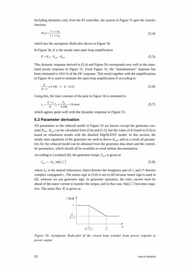
62 Risø-R-1500(EN)

Including dynamics only from the PI controller, the system in Figure 51 gets the transfer function

p

z

sssH

ωω

/1/1)(

++

= (5.4)

which has the asymptotic Bode plot shown in Figure 56.

In Figure 56, K is the steady state open loop amplification

gengenPP ΩKKK ⋅⋅= (5.5)

This dynamic response derived in (5.4) and Figure 56 corresponds very well to the simu-lated power response in Figure 51. Form Figure 51, the “instantaneous” response has been estimated to 18.6 % of the DC response. This result together with the amplifications in Figure 56 is used to estimate the open loop amplification K according to

23.0 186.01

=⇒≅+

KK

K (5.6)

Using this, the time constant of the pole in Figure 56 is estimated to

msec 54186.0

1=≅

+= iP

iPPTT

KK

τ (5.7)

which agrees quite well with the dynamic response in Figure 51.

5.3 Parameter derivation All parameters in the reduced model in Figure 55 are known except the generator con-stant Kgen. Kgen can be calculated from (5.6) and (5.5), but the value of K found in (5.6) is based on simulation results with the detailed DIgSILENT model. In this section, the steady state equations of the generator are used to derive Kgen, and as a result all parame-ters for the reduced model can be obtained from the generator data sheet and the control-ler parameters, which should all be available in wind turbine documentation.

According to Leonhard [8], the generator torque Tgen is given as

( )*Im3 rsmgen IILT −= (5.8)

where Lm is the mutual inductance, Im(x) denotes the imaginary part of x, and x* denotes complex conjugated x. The minus sign in (5.8) is not in [8] because motor sign is used in [8], whereas we use generator sign. In generator operation, the rotor current must be ahead of the stator current to transfer the torque, and in that case, Im(IsIr

*) becomes nega-tive. The stator flux Ψs is given as

ω

⎪H(ω)⎪

1

1+KK

( ) iPTKK

⋅+1 iPT1

Figure 56. Asymptotic Bode-plot of the closed loop transfer from power setpoint to power output

Risø-R-1500(EN) 63

rmsss ILILΨ += (5.9)

where Ls is the total stator inductance. Inserting Is from (5.9), (5.8) can be modified to

( )*Im3 rss

mgen IΨ

LLT −= (5.10)

In the stator flux coordinate system, ψs is per definition real ψs = ψsd, while Ir is complex I = Id + j Iq. Thus, in the stator flux coordinate system, the torque is given as

qds

mgen IΨ

LLT 3= (5.11)

The stator line-to-zero voltage Usl0 is given by

sessssl ΨjΩΨIRU ++=0 (5.12)

where Ωe = 2π⋅50 rad/s is the angular frequency of the electrical variables. Since the sta-tor resistance is relatively small, the first term in (5.12) is neglected. Moreover, in steady state, which is obtained as soon as the rotor current has reached the reference value, the second term in (5.12) becomes zero. Thus

03sn

sl e s e sdU U Ω Ψ ΩΨ≅ ≅ = (5.13)

where Usn is the rated voltage, assuming that the grid is ideal. Inserting ψsd from (5.13) in (5.11) yields

3 sn mgen rq

e s

U LT IΩ L

≅ (5.14)

For the sake of completeness, the inductances Lm and Ls are given by the main reactance Xm and the stator leakage reactance Xs in the generator data sheet according to

sems

mem

LjΩXXLjΩX=+

= (5.15)

Inserting (5.15) in (5.14) yields

ms

m

e

sn

rfq

gengen XX

XΩU

IT

K+

≅= 3 (5.16)

Thus, the steady state transfer Kgen from rotor current q-component Iq in the stator flux coordinate system to generator torque Tgen, can be assumed independent on the operation point, and it can be obtained from generator data sheet parameters according to (5.16).

Calculating according to (5.16) yields Kgen = 3.72 kNm/A. Using the estimate in (5.6) together with (5.5), and applying KPP and Ωgen in physical units, Kgen = 3.70 kNm/A is obtained.

The conclusion of this chapter is that the reduced model seems to represent the dynamics of the generator very well with a bandwidth of more than 20 Hz, which is a fully suffi-cient bandwidth of typical aeroelastic design models.

64 Risø-R-1500(EN)

6 Numerical optimization of PI-controller The numerical optimization code HAWTOPT has been used to investigate whether im-provement in regulation performance can be obtained using numerical tuning of the con-trol parameters Kp and Ki in the control algorithm described in Chapter 3. This optimi-zation code is a multipurpose optimization code that previously has been used for etc. optimization of aerodynamic blade layout, redistribution of blade stiffness and inertia for minimization of risk of edgewise blade vibrations, but until now pitch control parameters have not been included as optimization parameters, which is the new aspect in this inves-tigation. Using the optimization code the main control parameters Ki and Kp in the PI-regulation has been found based on an optimization strategy of minimization of the stan-dard deviation of the blade flapwise load signal.

The optimization is based on a 300 s time simulation at various wind speeds of power production with IEC turbulence. The simulation platform is HAWC even though Flex or other aeroelastic codes could have been used as well. At each wind speed the optimal parameters of Ki and Kp have been found. The objective function is minimization of the standard deviation of the blade root flapwise moment. Constraints of the design variables were some min. and max. values, but convergence was obtained after within 25 iterations without reaching these limits. Time consumption for optimisation of Kp and Ki at a sin-gle wind speed was app. 20 hours on a 3.0 GHz Pentium PC

6.1 Method HAWTOPT is a general multipurpose optimization code which handles execution of external programs, changes in input parameters through text files, execution of post processing programs and evaluation of the results in term of minimization or maximiza-tion of an object function. Several optimization methods can be chosen with this code. One method is the simplex optimization, which finds the nearest maxima or minima of an object function using gradients (the “hill-climbing” strategy). The method is rather fast but suffers from local maxima problems – the optimizations end when a local optima is found. Another method is the genetic algorithm [8], which is a completely different technique, based on ideas of biological gene and chromosome selection. The advantage of this method is especially that it is not restricted to local maxima, but on the cost of computational time. The method is computational more expensive than the simplex method.

Risø-R-1500(EN) 65

Figure 57: Route diagram of the optimization of control parameters using HAWTOPT.

6.2 Result Before optimization of parameters for all wind speeds some initial exercises were carried out at a single wind speed. The wind speed chosen was 15 m/s.

Initial exercises at 15 m/s

The first objective was to ensure that the optimization converges towards a solution, as shown in Figure 58, and that the results of the new parameters seemed reasonable (see Figure 59 and Figure 60).

The importance of simulation length is investigated in Figure 61, where significantly different parameters were obtained if only 60 s was used instead of 300 s. The conclu-sion of this was to use the full 300 s simulation.

In Figure 62 the importance of good initial value guesses was investigated. Optimization performance in term of iteration numbers was found with initial value parameters using the design method used in Chapter 3 (Kp=1.33, Ki=0.58), and rather arbitrary values of Kp=1.0 and Ki=1.0. It seems that both optimizations end up with the same results if many iterations were carried out, but the number of iterations before convergence was much less with the design method parameters.

In Figure 63 the choice of optimization method was investigated. This was done using 60 s simulations, which is the reason that the resulting parameters is not identical to the pa-rameters seen in the previous investigations. The genetic algorithm shows fastest con-vergence in term of iteration numbers, but as this method in itself is more time consum-ing per step the simplex algorithm is still the fastest. The converged result of the genetic algorithm was slightly different than the simplex algorithm, which indicates that the op-timization problem might be more non-linear than a simplex algorithm can handle. Never the less the simplex algorithm has still been used for the full 300 s simulation at every wind speed.

66 Risø-R-1500(EN)

Figure 58:Convergence reached at app. 20 iterations.

Figure 59: Time-series of flapwise blade root bending moment with initial control pa-rameters (top) and with control parameters after minimization of the standard deviation of this load (bottom).

Risø-R-1500(EN) 67

Figure 60: Time-series of rotor speed with initial control parameters (top) and optimized control parameters (bottom).

Figure 61: Illustration of importance of simulations length in the optimization. At only 60 s simulation the optimized values are significantly different that for 300 s.

68 Risø-R-1500(EN)

Figure 62:Illustration of importance of good initial value guesses. It seems that the two simulations reaches the same result if more iterations were carried out, but the conver-gence is obtained much sooner for the good initial values guess.

Figure 63:Difference in results as function of different optimization methods. The genetic algorithm shows best performance for this problem in terms op iterations steps. However since this method is rather time consuming the simplex algorithm is still the fastest.

Risø-R-1500(EN) 69

Optimization at several wind speeds using 300s. simulations.

Based on the initial investigations at 15 m/s a full range of optimizations covering the above rated wind speeds interval has been performed. The simulation length is 300 s and the optimization method is the simplex algorithm.

In Figure 64 the resulting PI-parameters can be seen as well as the object function and in Figure 65 performance of other sensors than the object function can be seen. What is interesting to notice is that the tendency in parameter is slightly higher proportional gains and slightly lower integral gains than what is the result of the design model. These changes lead to a bit “softer” regulation with higher standard deviation in the rotational speed. The tower base loading is also slightly reduced.

1.00

1.20

1.40

1.60

1.80

2.00

12 14 16 18 20 22 24 26

V (m/s)

Kp

Initial valuesOptimum

0.000

0.200

0.400

0.600

0.800

12 14 16 18 20 22 24 26

V (m/s)

Ki

Initial valueOptimum

Figure 64:Object function and initial and optimized values of Kp and Ki at the different wind speeds. The maximum improvement is seen to be at 14 m/s with a load reduction of 4 % in the standard deviation of flapwise blade root moment.

70 Risø-R-1500(EN)

Figure 65: Performance of other sensors than the object function. Values normalized by the standard deviation from the initial value simulations.

Risø-R-1500(EN) 71

6.3 Conclusion The main result of the optimization investigation is that numerical optimisation can be used to tune controller parameters, especially when the optimization is used as refine-ment of a qualified initial guess. Another result is that the design model used to calculate the initial value parameters, as described in Chapter 3, could not be refined much in terms of performance related to the flapwise blade moment. Numerical optimization of control parameters is not well suited for tuning from scratch. If the initial parameters are too far off track the simulation might not come through, or a not representative local maximum obtained. The last problem could very well be related to the chosen optimiza-tion method, where more future work could be done.

The improvement in flapwise load was app. 1-2% reduction in standard deviation. As an extra profit the tower base tilt moment was reduced with 2-3% in standard deviation. These improvements do not seem large, which is only an indication that the starting point was close to optimal.

Since the numerical optimisation uses many simulations and thereby large computational time it is essential to have fast, but still accurate, simulation codes. The present used ver-sion of HAWC might be in the upper end regarding time consumption for such use.

72 Risø-R-1500(EN)

References [1] Sørensen, P., Hansen, A. D., & Rosas, P. A. C, 2001, “Wind models for prediction

of power fluctuations from wind farms”, Proc. of ‘The Fifth Asia-Pacific Confer-ence on Wind Engineering (APCWEV)’, Kyoto, Japan, Journal of Wind Engineer-ing, no. 89, pp. 9-18.

[2] Sørensen, P., Hansen, A. D., Janosi, L., Bech, J., & Bak-Jensen, B., 2001, Simula-tion of interaction between wind farm and power system, Risø-R-1281, Risø Na-tional Laboratory.

[3] Hansen, A. D., Sørensen, P., Blaabjerg, F., & Bech, J., 2002, “Dynamic modelling of wind farm grid connection”, Wind Engineering, 26(4), pp. 191-208.

[4] Øye, S, 1991, “Dynamic stall - simulated as time lag of separation”, In Proceed-ings of the 4th IEA Symposium on the Aerodynamics of Wind Turbines, McAnulty, K. F (Ed.), Rome, Italy.

[5] Petersen, J. T., ”The Aeroelastic Code HawC - Model and Comparisons”, In 28th IEA Experts Meeting: State of the Art of Aeroelastic Codes, DTU, Lyngby, 1996.

[6] Mann, J., “Wind Field Simulation”, Prob. Eng. Mech., Elsevier Science, Vol. 13(4), pp. 269--283, 1998.

[7] Larsen, T. J., Description of the DLL Regulation Interface in HAWC, Risø-R-1290(EN), Risø National Laboratory, September 2001.

[8] Goldberg, David E., Genetic Algorithms in search, optimization & machine learn-ing, Addison-Wesley Publishing Co., Reading, Mass., USA, 1989.

74 Risø-R-1500(EN)

Appendix A HEAD HAWC input for "Aeroelastisk int. styring" /* data baseret diverse møller /* 80m tårnhøjde. kt/mh 23.09.2003 ; DEFINE_STRING CASE_IDENTIFICATION m01 ; DEFINE_STRING STRUCTURE_FILE_EXT 001 ; DEFINE_STRING AERODYN_FILE_EXT 001 ; DEFINE_STRING PROFILE_FILE_EXT 001 ; DEFINE_STRING GENERATOR_EFFICIENCY_FILE_EXT 001 ; DEFINE_STRING GEAR_BOX_EFFICIENCY_FILE_EXT 001 ; PARAMETERS TURBINE 3 2 1 2 ; PARAMETERS GEAR_BOX 85.0 2 1 ; PARAMETERS GENERATOR 150.0 9.99E3 2000.0 0.75 1500.0 1 ; PARAMETERS TILT 6.00 ; PARAMETERS HAM_DYNAMIC_STALL 1.50 6.00 0.75 0.14 * 0.53 0.30 0.70 0.95 1 12 ; ROTOR BASIC_LAYOUT 3 2 0.00 0.00 0.00 * 0.00 0.00 0.00 * 0.00 0.00 0.00 0.0 ; DAMPING TOWER 0.0 0.0 0.0 3.06E-3 3.06E-3 1.45E-3 ; DAMPING SHAFT 0.0 0.0 0.0 1.00E-3 1.00E-3 3.20E-3 ; DAMPING BLADE 0.0 0.0 0.0 1.39E-3 9.00E-4 1.39E-3 ; DEFINITION AEROCAL_INDUCTION 32 1.0 1.0 1.0 0.1 1.0 * 4.0 4.0 4.0 0.4 4.0 * 2.0 2.0 2.0 2.0 1.0 ; ; DEFINITION AEROCAL_MODIFICATIONS 1 1 15 ; DEFINITION WIND_FIELD 1.25 9.00 80.00 0.00 0.00 0.00 0.01 1 ; DEFINITION TOWER_AERODYNAMIC_LOAD 0.6; DEFINITION TOWER_SHADOW 1.200 2.150 1.5 1 ; ; Blade nodes NODE BLADE 1 1 0.000 0.000 0.000 ; NODE BLADE 1 2 0.000 0.000 2.000 ; NODE BLADE 1 3 0.000 0.000 7.000 ; NODE BLADE 1 4 0.000 0.000 12.000 ; NODE BLADE 1 5 0.000 0.000 20.000 ; NODE BLADE 1 6 0.000 0.000 25.000 ; NODE BLADE 1 7 0.000 0.000 28.000 ; NODE BLADE 1 8 0.000 0.000 31.000 ; NODE BLADE 1 9 0.000 0.000 34.000 ; NODE BLADE 1 10 0.000 0.000 36.000 ; NODE BLADE 1 11 0.000 0.000 38.000 ; NODE BLADE 1 12 0.000 0.000 40.000 ; NODE BLADE 2 1 0.000 0.000 0.000 ; NODE BLADE 2 2 0.000 0.000 2.000 ; NODE BLADE 2 3 0.000 0.000 7.000 ; NODE BLADE 2 4 0.000 0.000 12.000 ; NODE BLADE 2 5 0.000 0.000 20.000 ; NODE BLADE 2 6 0.000 0.000 25.000 ; NODE BLADE 2 7 0.000 0.000 28.000 ; NODE BLADE 2 8 0.000 0.000 31.000 ; NODE BLADE 2 9 0.000 0.000 34.000 ; NODE BLADE 2 10 0.000 0.000 36.000 ; NODE BLADE 2 11 0.000 0.000 38.000 ; NODE BLADE 2 12 0.000 0.000 40.000 ; NODE BLADE 3 1 0.000 0.000 0.000 ; NODE BLADE 3 2 0.000 0.000 2.000 ; NODE BLADE 3 3 0.000 0.000 7.000 ; NODE BLADE 3 4 0.000 0.000 12.000 ; NODE BLADE 3 5 0.000 0.000 20.000 ; NODE BLADE 3 6 0.000 0.000 25.000 ; NODE BLADE 3 7 0.000 0.000 28.000 ; NODE BLADE 3 8 0.000 0.000 31.000 ; NODE BLADE 3 9 0.000 0.000 34.000 ; NODE BLADE 3 10 0.000 0.000 36.000 ; NODE BLADE 3 11 0.000 0.000 38.000 ; NODE BLADE 3 12 0.000 0.000 40.000 ; ; Nacelle nodes NODE NACELLE 1 0.0 0.000 0.000 ; Tower top NODE NACELLE 2 0.0 -0.600 0.000 ; Gearbox NODE NACELLE 3 0.0 -2.186 0.000 ; Main shaft flange NODE NACELLE 4 0.0 -3.486 0.000 ; Rotor centre ; Tower nodes NODE TOWER 1 0.000 0.000 0.000 ; NODE TOWER 2 0.000 0.000 -20.000 ; NODE TOWER 3 0.000 0.000 -40.000 ; NODE TOWER 4 0.000 0.000 -60.000 ; NODE TOWER 5 0.000 0.000 -76.000 ; NODE TOWER 6 0.000 0.000 -80.000 ; DEFINITION CONCENTRATED_MASS 1 5 2 75.3E+3 409.4E+3 20.0E+3 367.7E+3 ; TYPES BLADE_AERODYN_3 1 1 1 ; TYPES BLADE_STRUCTURE_3 1 1 1 ; TYPES SHAFT_STRUCTURE 1 ;

Risø-R-1500(EN) 75

TYPES TOWER_STRUCTURE 1 ; TYPES USE_CALCULATED_BEAMS ; INITIAL AZIMUTH 0.000 1.85 0.000 ; ; WRITE BEAM_DATA_TO_RDA_DIRECTORY ; RESULTS BLADE_CO_SYS_FORCE 1 ; RESULTS BLADE_CO_SYS_DEFORM 1 ; RESULTS FORCE_MOMENT_SIGN 4 ; RESULTS RESPONSE_TIME_OFFSET 10.0; RESULTS TIME ; RESULTS AZIMUTH 0.0 ; RESULTS ROTOR_SPEED ; RESULTS ELECTRICAL_POWER ; RESULTS WIND_SPEED_AT_HUB 1 1 1 1 1 ; RESULTS PITCH_BEARING_ANGLE 1 1 1 ; RESULTS BLADE_FORCE_MOMENT 1 1 0 0 0 1 1 0 ; Rotor centre RESULTS BLADE_FORCE_MOMENT 1 2 0 0 0 1 1 0 ; R=1.2m RESULTS BLADE_FORCE_MOMENT 1 5 0 0 0 1 1 0 ; r=20m RESULTS BLADE_FORCE_MOMENT 1 9 0 0 0 1 1 0 ; r=34m RESULTS SHAFT_FORCE_MOMENT 4 0 1 0 1 1 1 ; Rotor centre RESULTS TOWER_FORCE_MOMENT 1 1 1 0 1 1 1 ; Tower base RESULTS TOWER_FORCE_MOMENT 2 1 1 0 1 1 1 ; Tower h=25m RESULTS TOWER_FORCE_MOMENT 4 1 1 0 1 1 1 ; Tower top RESULTS BLADE_DEFORMATION 1 12 1 1 0 0 0 0 ; Tip RESULTS SHAFT_DEFORMATION 4 1 0 1 0 0 0 ; Rotor centre RESULTS TOWER_DEFORMATION 4 1 1 0 0 0 0 ; Tower top DEFINITION RESPONSE_CALC_LIMITS 1.0E-3 1.0E-3 0.0 5.0E-1 1 10 ; WRITE POWER 7.0 25.0 1.0 4 1 0.10 0.10 0.10 8 ; ; WRITE RESPONSE 30.0 0.025 1 1 0 1 2 1 5 1 ; STOP ;

76 Risø-R-1500(EN)

Appendix B 1 1 1 1 BLADES 1 24 R m xcg ycg ri_x ri_y x_sh y_sh E G I_x I_y I_p k_x k_y A Str. pitch 0.000 2.940E+03 0.0 0.0 1.000E-03 1.000E-03 0.000 0.000 2.10E+11 8.10E+10 9.790E+01 9.790E+01 9.790E+01 0.5 0.5 0.8830 0.00 2.000 2.940E+03 0.0 0.0 1.000E-03 1.000E-03 0.000 0.000 2.10E+11 8.10E+10 9.790E+01 9.790E+01 9.790E+01 0.5 0.5 0.8830 0.00 2.001 1.066E+03 0.0 0.0 2.430E-01 2.180E-01 0.000 0.000 4.00E+10 1.50E+10 5.860E-02 5.909E-02 1.174E-01 0.5 0.5 0.5960 16.00 3.200 1.166E+03 0.0 0.0 3.430E-01 3.180E-01 0.000 0.000 4.00E+10 1.50E+10 6.860E-02 5.909E-02 1.274E-01 0.5 0.5 0.5960 26.00 4.200 4.626E+02 0.0 0.0 5.350E-01 5.130E-01 0.000 0.000 4.00E+10 1.50E+10 6.615E-02 6.076E-02 1.274E-01 0.5 0.5 0.2360 11.00 5.700 4.635E+02 0.0 0.0 5.210E-01 5.230E-01 0.000 0.000 4.00E+10 1.50E+10 6.301E-02 6.350E-02 1.264E-01 0.5 0.5 0.2360 14.10 7.700 4.371E+02 0.0 0.0 4.870E-01 5.920E-01 0.000 0.000 4.00E+10 1.50E+10 5.194E-02 7.673E-02 1.284E-01 0.5 0.5 0.2230 17.57 10.200 3.646E+02 0.0 0.0 4.070E-01 6.320E-01 0.236 0.024 4.00E+10 1.50E+10 3.018E-02 7.281E-02 1.029E-01 0.8 0.4 0.1860 19.92 12.200 3.146E+02 0.0 0.0 3.770E-01 5.910E-01 0.274 0.010 4.00E+10 1.50E+10 2.244E-02 5.488E-02 7.732E-02 0.9 0.4 0.1600 17.36 14.200 2.822E+02 0.0 0.0 3.570E-01 5.740E-01 0.268 0.007 4.00E+10 1.50E+10 1.793E-02 4.655E-02 6.448E-02 1.0 0.4 0.1440 14.79 16.200 2.724E+02 0.0 0.0 3.220E-01 5.520E-01 0.259 0.006 4.00E+10 1.50E+10 1.411E-02 4.145E-02 5.557E-02 0.8 0.4 0.1390 11.89 18.200 2.587E+02 0.0 0.0 2.670E-01 5.300E-01 0.248 0.006 4.00E+10 1.50E+10 9.241E-03 3.626E-02 4.547E-02 0.8 0.4 0.1320 9.30 20.200 2.391E+02 0.0 0.0 2.190E-01 4.750E-01 0.236 0.005 4.00E+10 1.50E+10 5.713E-03 2.695E-02 3.263E-02 0.8 0.4 0.1220 7.24 22.200 2.185E+02 0.0 0.0 1.810E-01 4.030E-01 0.223 0.004 4.00E+10 1.50E+10 3.577E-03 1.774E-02 2.136E-02 0.8 0.4 0.1110 5.59 24.200 2.019E+02 0.0 0.0 1.520E-01 3.370E-01 0.210 0.002 4.00E+10 1.50E+10 2.332E-03 1.146E-02 1.381E-02 0.8 0.4 0.1030 4.28 26.200 1.793E+02 0.0 0.0 1.310E-01 3.040E-01 0.197 0.002 4.00E+10 1.50E+10 1.528E-03 8.281E-03 9.800E-03 0.8 0.4 0.0913 3.26 28.200 1.597E+02 0.0 0.0 1.100E-01 2.720E-01 0.184 0.001 4.00E+10 1.50E+10 9.633E-04 5.909E-03 6.870E-03 0.8 0.4 0.0817 2.40 30.200 1.421E+02 0.0 0.0 9.900E-02 2.440E-01 0.170 0.001 4.00E+10 1.50E+10 7.007E-04 4.243E-03 4.939E-03 0.8 0.4 0.0727 1.66 32.200 1.185E+02 0.0 0.0 8.400E-02 2.300E-01 0.155 0.001 4.00E+10 1.50E+10 4.214E-04 3.136E-03 3.557E-03 0.8 0.4 0.0605 1.04 34.200 8.859E+01 0.0 0.0 7.200E-02 2.090E-01 0.142 0.001 4.00E+10 1.50E+10 2.274E-04 1.940E-03 2.166E-03 0.8 0.4 0.0452 0.63 36.200 6.282E+01 0.0 0.0 5.800E-02 1.980E-01 0.080 0.000 4.00E+10 1.50E+10 1.048E-04 1.234E-03 1.342E-03 0.8 0.4 0.0321 0.34 38.200 3.822E+01 0.0 0.0 3.800E-02 1.260E-01 0.030 0.000 4.00E+10 1.50E+10 2.724E-05 3.018E-04 3.283E-04 0.8 0.4 0.0195 0.18 39.200 2.842E+01 0.0 0.0 2.100E-02 1.040E-01 0.010 0.000 4.00E+10 1.50E+10 6.007E-06 1.548E-04 1.607E-04 0.8 0.4 0.0145 0.82 40.000 2.234E+01 0.0 0.0 5.000E-03 2.400E-02 0.000 0.000 4.00E+10 1.50E+10 2.548E-07 6.223E-06 6.478E-06 0.8 0.4 0.0114 6.34 1 SHAFT 1 6 R m xcg ycg ri_x ri_y x_sh y_sh E G I_x I_y I_p k_x k_y A Str. pitch 0.000 9.800E-01 0.0 0.0 1.000E-03 1.000E-03 0.000 0.000 2.10E+11 8.10E+10 1.960E-02 1.960E-02 1.136E-03 0.5 0.5 0.2870 0.00 0.600 9.800E-01 0.0 0.0 1.000E-03 1.000E-03 0.000 0.000 2.10E+11 8.10E+10 1.960E-02 1.960E-02 1.136E-03 0.5 0.5 0.2870 0.00 0.600 9.800E-01 0.0 0.0 1.000E-03 1.000E-03 0.000 0.000 2.10E+11 8.10E+10 6.791E-03 6.791E-03 1.362E-02 0.5 0.5 0.2870 0.00 2.186 9.800E-01 0.0 0.0 1.000E-03 1.000E-03 0.000 0.000 2.10E+11 8.10E+10 6.791E-03 6.791E-03 1.362E-02 0.5 0.5 0.2870 0.00 2.186 9.800E-01 0.0 0.0 1.000E-03 1.000E-03 0.000 0.000 2.10E+11 8.10E+10 9.790E+01 9.790E+01 9.790E+01 0.5 0.5 0.9990 0.00 3.486 9.800E-01 0.0 0.0 1.000E-03 1.000E-03 0.000 0.000 2.10E+11 8.10E+10 9.790E+01 9.790E+01 9.790E+01 0.5 0.5 0.9990 0.00 1 TOWER 1 83 R m xcg ycg ri_x ri_y x_sh y_sh E G I_x I_y I_p k_x k_y A Str. pitch 0.000 6.203E+03 0.0 0.0 1.066E+00 1.066E+00 0.000 0.000 2.10E+11 8.10E+10 8.987E-01 8.987E-01 1.793E+00 0.5 0.5 0.8070 0.00 0.982 3.097E+03 0.0 0.0 1.510E+00 1.510E+00 0.000 0.000 2.10E+11 8.10E+10 8.987E-01 8.987E-01 1.793E+00 0.5 0.5 0.4020 0.00 1.964 3.097E+03 0.0 0.0 1.510E+00 1.510E+00 0.000 0.000 2.10E+11 8.10E+10 8.987E-01 8.987E-01 1.793E+00 0.5 0.5 0.4020 0.00 2.945 3.097E+03 0.0 0.0 1.510E+00 1.510E+00 0.000 0.000 2.10E+11 8.10E+10 8.987E-01 8.987E-01 1.793E+00 0.5 0.5 0.4020 0.00 3.927 3.097E+03 0.0 0.0 1.510E+00 1.510E+00 0.000 0.000 2.10E+11 8.10E+10 8.987E-01 8.987E-01 1.793E+00 0.5 0.5 0.4020 0.00 4.909 3.097E+03 0.0 0.0 1.510E+00 1.510E+00 0.000 0.000 2.10E+11 8.10E+10 8.987E-01 8.987E-01 1.793E+00 0.5 0.5 0.4020 0.00 5.891 3.097E+03 0.0 0.0 1.510E+00 1.510E+00 0.000 0.000 2.10E+11 8.10E+10 8.987E-01 8.987E-01 1.793E+00 0.5 0.5 0.4020 0.00

Risø-R-1500(EN) 77

6.872 3.097E+03 0.0 0.0 1.510E+00 1.510E+00 0.000 0.000 2.10E+11 8.10E+10 8.987E-01 8.987E-01 1.793E+00 0.5 0.5 0.4020 0.00 7.854 3.097E+03 0.0 0.0 1.510E+00 1.510E+00 0.000 0.000 2.10E+11 8.10E+10 8.987E-01 8.987E-01 1.793E+00 0.5 0.5 0.4020 0.00 8.836 3.097E+03 0.0 0.0 1.510E+00 1.510E+00 0.000 0.000 2.10E+11 8.10E+10 8.987E-01 8.987E-01 1.793E+00 0.5 0.5 0.4020 0.00 9.818 3.097E+03 0.0 0.0 1.510E+00 1.510E+00 0.000 0.000 2.10E+11 8.10E+10 8.987E-01 8.987E-01 1.793E+00 0.5 0.5 0.4020 0.00 10.790 2.891E+03 0.0 0.0 1.510E+00 1.510E+00 0.000 0.000 2.10E+11 8.10E+10 8.399E-01 8.399E-01 1.676E+00 0.5 0.5 0.3760 0.00 11.780 2.685E+03 0.0 0.0 1.511E+00 1.511E+00 0.000 0.000 2.10E+11 8.10E+10 7.811E-01 7.811E-01 1.558E+00 0.5 0.5 0.3490 0.00 12.760 2.479E+03 0.0 0.0 1.512E+00 1.512E+00 0.000 0.000 2.10E+11 8.10E+10 7.223E-01 7.223E-01 1.441E+00 0.5 0.5 0.3220 0.00 13.740 2.479E+03 0.0 0.0 1.512E+00 1.512E+00 0.000 0.000 2.10E+11 8.10E+10 7.223E-01 7.223E-01 1.441E+00 0.5 0.5 0.3220 0.00 14.720 2.479E+03 0.0 0.0 1.512E+00 1.512E+00 0.000 0.000 2.10E+11 8.10E+10 7.223E-01 7.223E-01 1.441E+00 0.5 0.5 0.3220 0.00 15.700 2.479E+03 0.0 0.0 1.512E+00 1.512E+00 0.000 0.000 2.10E+11 8.10E+10 7.223E-01 7.223E-01 1.441E+00 0.5 0.5 0.3220 0.00 16.690 2.274E+03 0.0 0.0 1.513E+00 1.513E+00 0.000 0.000 2.10E+11 8.10E+10 6.625E-01 6.625E-01 1.323E+00 0.5 0.5 0.2960 0.00 17.670 2.274E+03 0.0 0.0 1.513E+00 1.513E+00 0.000 0.000 2.10E+11 8.10E+10 6.625E-01 6.625E-01 1.323E+00 0.5 0.5 0.2960 0.00 18.650 5.390E+03 0.0 0.0 9.830E-01 9.830E-01 0.000 0.000 2.10E+11 8.10E+10 6.625E-01 6.625E-01 1.323E+00 0.5 0.5 0.7000 0.00 19.640 2.264E+03 0.0 0.0 1.505E+00 1.505E+00 0.000 0.000 2.10E+11 8.10E+10 6.527E-01 6.527E-01 1.303E+00 0.5 0.5 0.2940 0.00 20.620 2.244E+03 0.0 0.0 1.493E+00 1.493E+00 0.000 0.000 2.10E+11 8.10E+10 6.380E-01 6.380E-01 1.274E+00 0.5 0.5 0.2920 0.00 21.600 2.225E+03 0.0 0.0 1.481E+00 1.481E+00 0.000 0.000 2.10E+11 8.10E+10 6.223E-01 6.223E-01 1.245E+00 0.5 0.5 0.2900 0.00 22.580 2.215E+03 0.0 0.0 1.470E+00 1.470E+00 0.000 0.000 2.10E+11 8.10E+10 6.076E-01 6.076E-01 1.215E+00 0.5 0.5 0.2870 0.00 23.560 2.195E+03 0.0 0.0 1.458E+00 1.458E+00 0.000 0.000 2.10E+11 8.10E+10 5.939E-01 5.939E-01 1.186E+00 0.5 0.5 0.2850 0.00 24.540 2.176E+03 0.0 0.0 1.446E+00 1.446E+00 0.000 0.000 2.10E+11 8.10E+10 5.792E-01 5.792E-01 1.156E+00 0.5 0.5 0.2830 0.00 25.530 2.156E+03 0.0 0.0 1.434E+00 1.434E+00 0.000 0.000 2.10E+11 8.10E+10 5.655E-01 5.655E-01 1.127E+00 0.5 0.5 0.2800 0.00 26.510 2.136E+03 0.0 0.0 1.422E+00 1.422E+00 0.000 0.000 2.10E+11 8.10E+10 5.508E-01 5.508E-01 1.098E+00 0.5 0.5 0.2780 0.00 27.490 2.117E+03 0.0 0.0 1.411E+00 1.411E+00 0.000 0.000 2.10E+11 8.10E+10 5.380E-01 5.380E-01 1.078E+00 0.5 0.5 0.2760 0.00 28.470 2.107E+03 0.0 0.0 1.399E+00 1.399E+00 0.000 0.000 2.10E+11 8.10E+10 5.243E-01 5.243E-01 1.049E+00 0.5 0.5 0.2730 0.00 29.450 2.087E+03 0.0 0.0 1.387E+00 1.387E+00 0.000 0.000 2.10E+11 8.10E+10 5.116E-01 5.116E-01 1.019E+00 0.5 0.5 0.2710 0.00 30.430 2.068E+03 0.0 0.0 1.375E+00 1.375E+00 0.000 0.000 2.10E+11 8.10E+10 4.978E-01 4.978E-01 9.996E-01 0.5 0.5 0.2690 0.00 31.420 2.048E+03 0.0 0.0 1.363E+00 1.363E+00 0.000 0.000 2.10E+11 8.10E+10 4.851E-01 4.851E-01 9.712E-01 0.5 0.5 0.2670 0.00 32.400 2.029E+03 0.0 0.0 1.352E+00 1.352E+00 0.000 0.000 2.10E+11 8.10E+10 4.733E-01 4.733E-01 9.457E-01 0.5 0.5 0.2640 0.00 33.380 2.019E+03 0.0 0.0 1.340E+00 1.340E+00 0.000 0.000 2.10E+11 8.10E+10 4.606E-01 4.606E-01 9.212E-01 0.5 0.5 0.2620 0.00 34.360 1.813E+03 0.0 0.0 1.329E+00 1.329E+00 0.000 0.000 2.10E+11 8.10E+10 4.087E-01 4.087E-01 8.173E-01 0.5 0.5 0.2360 0.00 35.340 1.803E+03 0.0 0.0 1.317E+00 1.317E+00 0.000 0.000 2.10E+11 8.10E+10 3.979E-01 3.979E-01 7.958E-01 0.5 0.5 0.2340 0.00 36.330 1.784E+03 0.0 0.0 1.305E+00 1.305E+00 0.000 0.000 2.10E+11 8.10E+10 3.871E-01 3.871E-01 7.742E-01 0.5 0.5 0.2320 0.00 37.310 1.764E+03 0.0 0.0 1.293E+00 1.293E+00 0.000 0.000 2.10E+11 8.10E+10 3.763E-01 3.763E-01 7.536E-01 0.5 0.5 0.2300 0.00 38.290 1.754E+03 0.0 0.0 1.281E+00 1.281E+00 0.000 0.000 2.10E+11 8.10E+10 3.665E-01 3.665E-01 7.330E-01 0.5 0.5 0.2280 0.00 39.270 1.735E+03 0.0 0.0 1.270E+00 1.270E+00 0.000 0.000 2.10E+11 8.10E+10 3.567E-01 3.567E-01 7.125E-01 0.5 0.5 0.2260 0.00 40.250 1.715E+03 0.0 0.0 1.258E+00 1.258E+00 0.000 0.000 2.10E+11 8.10E+10 3.469E-01 3.469E-01 6.929E-01 0.5 0.5 0.2240 0.00 41.230 1.705E+03 0.0 0.0 1.246E+00 1.246E+00 0.000 0.000 2.10E+11 8.10E+10 3.371E-01 3.371E-01 6.742E-01 0.5 0.5 0.2210 0.00 42.220 3.793E+03 0.0 0.0 8.230E-01 8.230E-01 0.000 0.000 2.10E+11 8.10E+10 3.273E-01 3.273E-01 6.546E-01 0.5 0.5 0.4930 0.00 43.200 1.676E+03 0.0 0.0 1.223E+00 1.223E+00 0.000 0.000 2.10E+11 8.10E+10 3.185E-01 3.185E-01 6.370E-01 0.5 0.5 0.2170 0.00 44.180 1.656E+03 0.0 0.0 1.212E+00 1.212E+00 0.000 0.000 2.10E+11 8.10E+10 3.107E-01 3.107E-01 6.203E-01 0.5 0.5 0.2150 0.00 45.160 1.646E+03 0.0 0.0 1.202E+00 1.202E+00 0.000 0.000 2.10E+11 8.10E+10 3.018E-01 3.018E-01 6.047E-01 0.5 0.5 0.2140 0.00 46.140 1.627E+03 0.0 0.0 1.191E+00 1.191E+00 0.000 0.000 2.10E+11 8.10E+10 2.940E-01 2.940E-01 5.880E-01 0.5 0.5 0.2120 0.00 47.130 1.617E+03 0.0 0.0 1.180E+00 1.180E+00 0.000 0.000 2.10E+11 8.10E+10 2.862E-01 2.862E-01 5.723E-01 0.5 0.5 0.2100 0.00 48.110 1.597E+03 0.0 0.0 1.169E+00 1.169E+00 0.000 0.000 2.10E+11 8.10E+10 2.783E-01 2.783E-01 5.566E-01 0.5 0.5 0.2080 0.00 49.090 1.431E+03 0.0 0.0 1.159E+00 1.159E+00 0.000 0.000 2.10E+11 8.10E+10 2.440E-01 2.440E-01 4.880E-01 0.5 0.5 0.1850 0.00 50.070 1.411E+03 0.0 0.0 1.148E+00 1.148E+00 0.000 0.000 2.10E+11 8.10E+10 2.372E-01 2.372E-01 4.743E-01 0.5 0.5 0.1840 0.00 51.050 1.401E+03 0.0 0.0 1.137E+00 1.137E+00 0.000 0.000 2.10E+11 8.10E+10 2.303E-01 2.303E-01 4.616E-01 0.5 0.5 0.1820 0.00 52.030 1.382E+03 0.0 0.0 1.127E+00 1.127E+00 0.000 0.000 2.10E+11 8.10E+10 2.244E-01 2.244E-01 4.488E-01 0.5 0.5 0.1800 0.00 53.010 1.372E+03 0.0 0.0 1.116E+00 1.116E+00 0.000 0.000 2.10E+11 8.10E+10 2.176E-01 2.176E-01 4.351E-01 0.5 0.5 0.1780 0.00 54.000 1.362E+03 0.0 0.0 1.105E+00 1.105E+00 0.000 0.000 2.10E+11 8.10E+10 2.117E-01 2.117E-01 4.234E-01 0.5 0.5 0.1770 0.00 54.980 1.343E+03 0.0 0.0 1.094E+00 1.094E+00 0.000 0.000 2.10E+11 8.10E+10 2.058E-01 2.058E-01 4.106E-01 0.5 0.5 0.1750 0.00 55.960 1.333E+03 0.0 0.0 1.083E+00 1.083E+00 0.000 0.000 2.10E+11 8.10E+10 1.989E-01 1.989E-01 3.989E-01 0.5 0.5 0.1730 0.00 56.940 1.323E+03 0.0 0.0 1.073E+00 1.073E+00 0.000 0.000 2.10E+11 8.10E+10 1.931E-01 1.931E-01 3.871E-01 0.5 0.5 0.1720 0.00

78 Risø-R-1500(EN)

57.920 1.166E+03 0.0 0.0 1.063E+00 1.063E+00 0.000 0.000 2.10E+11 8.10E+10 1.676E-01 1.676E-01 3.342E-01 0.5 0.5 0.1510 0.00 58.910 1.147E+03 0.0 0.0 1.052E+00 1.052E+00 0.000 0.000 2.10E+11 8.10E+10 1.617E-01 1.617E-01 3.244E-01 0.5 0.5 0.1500 0.00 59.890 1.137E+03 0.0 0.0 1.041E+00 1.041E+00 0.000 0.000 2.10E+11 8.10E+10 1.568E-01 1.568E-01 3.146E-01 0.5 0.5 0.1480 0.00 60.870 1.127E+03 0.0 0.0 1.030E+00 1.030E+00 0.000 0.000 2.10E+11 8.10E+10 1.519E-01 1.519E-01 3.048E-01 0.5 0.5 0.1460 0.00 61.850 1.117E+03 0.0 0.0 1.019E+00 1.019E+00 0.000 0.000 2.10E+11 8.10E+10 1.480E-01 1.480E-01 2.950E-01 0.5 0.5 0.1450 0.00 62.830 1.107E+03 0.0 0.0 1.009E+00 1.009E+00 0.000 0.000 2.10E+11 8.10E+10 1.431E-01 1.431E-01 2.862E-01 0.5 0.5 0.1430 0.00 63.810 1.088E+03 0.0 0.0 9.980E-01 9.980E-01 0.000 0.000 2.10E+11 8.10E+10 1.382E-01 1.382E-01 2.764E-01 0.5 0.5 0.1420 0.00 64.800 1.078E+03 0.0 0.0 9.870E-01 9.870E-01 0.000 0.000 2.10E+11 8.10E+10 1.343E-01 1.343E-01 2.675E-01 0.5 0.5 0.1400 0.00 65.780 1.068E+03 0.0 0.0 9.760E-01 9.760E-01 0.000 0.000 2.10E+11 8.10E+10 1.294E-01 1.294E-01 2.597E-01 0.5 0.5 0.1390 0.00 66.760 9.241E+02 0.0 0.0 9.660E-01 9.660E-01 0.000 0.000 2.10E+11 8.10E+10 1.097E-01 1.097E-01 2.195E-01 0.5 0.5 0.1200 0.00 67.740 9.143E+02 0.0 0.0 9.550E-01 9.550E-01 0.000 0.000 2.10E+11 8.10E+10 1.058E-01 1.058E-01 2.127E-01 0.5 0.5 0.1190 0.00 68.720 9.036E+02 0.0 0.0 9.450E-01 9.450E-01 0.000 0.000 2.10E+11 8.10E+10 1.029E-01 1.029E-01 2.058E-01 0.5 0.5 0.1170 0.00 69.710 8.938E+02 0.0 0.0 9.340E-01 9.340E-01 0.000 0.000 2.10E+11 8.10E+10 9.898E-02 9.898E-02 1.989E-01 0.5 0.5 0.1160 0.00 70.690 8.830E+02 0.0 0.0 9.230E-01 9.230E-01 0.000 0.000 2.10E+11 8.10E+10 9.584E-02 9.584E-02 1.921E-01 0.5 0.5 0.1150 0.00 71.670 8.732E+02 0.0 0.0 9.120E-01 9.120E-01 0.000 0.000 2.10E+11 8.10E+10 9.251E-02 9.251E-02 1.852E-01 0.5 0.5 0.1130 0.00 72.650 8.624E+02 0.0 0.0 9.010E-01 9.010E-01 0.000 0.000 2.10E+11 8.10E+10 8.928E-02 8.928E-02 1.784E-01 0.5 0.5 0.1120 0.00 73.630 8.526E+02 0.0 0.0 8.910E-01 8.910E-01 0.000 0.000 2.10E+11 8.10E+10 8.604E-02 8.604E-02 1.725E-01 0.5 0.5 0.1110 0.00 74.610 9.614E+02 0.0 0.0 8.790E-01 8.790E-01 0.000 0.000 2.10E+11 8.10E+10 9.467E-02 9.467E-02 1.891E-01 0.5 0.5 0.1250 0.00 75.600 9.496E+02 0.0 0.0 8.680E-01 8.680E-01 0.000 0.000 2.10E+11 8.10E+10 9.114E-02 9.114E-02 1.823E-01 0.5 0.5 0.1230 0.00 76.580 1.058E+03 0.0 0.0 8.570E-01 8.570E-01 0.000 0.000 2.10E+11 8.10E+10 9.898E-02 9.898E-02 1.970E-01 0.5 0.5 0.1370 0.00 77.560 1.039E+03 0.0 0.0 8.460E-01 8.460E-01 0.000 0.000 2.10E+11 8.10E+10 9.486E-02 9.486E-02 1.901E-01 0.5 0.5 0.1350 0.00 78.540 1.666E+03 0.0 0.0 6.550E-01 6.550E-01 0.000 0.000 2.10E+11 8.10E+10 9.134E-02 9.134E-02 1.823E-01 0.5 0.5 0.2170 0.00 78.540 9.800E-01 0.0 0.0 1.000E-03 1.000E-03 0.000 0.000 2.10E+11 8.10E+10 9.790E+05 9.790E+05 9.790E+05 0.5 0.5 9.9900 0.00 80.100 9.800E-01 0.0 0.0 1.000E-03 1.000E-03 0.000 0.000 2.10E+11 8.10E+10 9.790E+05 9.790E+05 9.790E+05 0.5 0.5 9.9900 0.00

80 Risø-R-1500(EN)

Appendix C 1 40 m rotorradius 1 14 ch th twist x_ae y_ae PC set 0.000 0.001 100.000 0.000 0.000 0.000 1 1.200 2.450 100.000 5.100 0.000 0.000 1 5.200 2.650 80.000 6.700 0.000 0.000 1 9.200 3.000 52.000 9.400 0.000 0.000 1 13.200 3.200 33.000 9.400 0.000 0.000 1 17.200 2.800 26.000 5.400 0.000 0.000 1 21.200 2.400 22.200 3.500 0.000 0.000 1 25.200 2.000 20.000 2.300 0.000 0.000 1 29.200 1.800 19.000 1.300 0.000 0.000 1 33.200 1.550 18.500 0.500 0.000 0.000 1 37.200 1.180 18.000 0.000 0.000 0.000 1 39.200 0.620 16.300 1.000 0.000 0.000 1 39.600 0.400 15.700 2.400 0.000 0.000 1 40.000 0.010 15.000 6.000 0.000 0.000 1

Risø-R-1500(EN) 81

Appendix D 1 Converted format 7 NACA 634xx 1 35 15.00000 NACA 63415, Modified to Re = 6 million -180.00000 0.00000 0.10000 0.00000 -170.00000 0.80000 0.24000 0.40000 -150.00000 0.80000 0.58000 0.32500 -120.00000 0.49000 1.06000 0.32500 -90.00000 -0.11400 1.30000 0.32500 -60.00000 -0.75500 1.06000 0.32500 -30.00000 -1.20000 0.45000 0.22000 -20.00000 -1.20000 0.20000 0.05000 -15.00000 -1.10000 0.10000 0.00000 -10.00000 -0.82000 0.01200 0.00000 -6.00000 -0.36500 0.00900 -0.03750 -2.00000 0.08570 0.00600 -0.06600 2.00000 0.54610 0.00600 -0.07800 4.00000 0.77630 0.00650 -0.08400 6.00000 0.99500 0.00960 -0.09000 8.00000 1.17000 0.01320 -0.09000 10.00000 1.31400 0.01690 -0.09000 12.00000 1.44500 0.02350 -0.09000 14.00000 1.45500 0.04700 -0.09000 16.00000 1.44830 0.08200 -0.09000 18.00000 1.36660 0.12424 -0.09670 20.00000 1.32500 0.17700 -0.10330 25.00000 1.25906 0.32423 -0.12000 30.00000 1.19000 0.47536 -0.14000 40.00000 1.06000 0.69000 -0.18000 50.00000 0.93000 0.90000 -0.22000 60.00000 0.75500 1.06000 -0.26000 70.00000 0.55500 1.18000 -0.29250 80.00000 0.34000 1.26000 -0.32500 90.00000 0.11400 1.30000 -0.32500 100.00000 -0.11000 1.27000 -0.32500 120.00000 -0.49000 1.06000 -0.32500 150.00000 -0.80000 0.58000 -0.32500 170.00000 -0.80000 0.24000 -0.40000 180.00000 0.00000 0.10000 0.00000 2 35 18.00000 NACA 63418, Modified to Re = 6 million -180.00000 0.00000 0.10000 0.00000 -170.00000 0.80000 0.24000 0.40000 -150.00000 0.80000 0.58000 0.32500 -120.00000 0.49000 1.06000 0.32500 -90.00000 -0.11400 1.30000 0.32500 -60.00000 -0.75500 1.06000 0.32500 -30.00000 -1.20000 0.45000 0.22000 -20.00000 -1.20000 0.20000 0.05000 -15.00000 -1.10000 0.10000 0.00000 -10.00000 -0.82000 0.01200 0.00000 -6.00000 -0.36500 0.00900 -0.03750 -2.00000 0.08140 0.00600 -0.06600 2.00000 0.54710 0.00600 -0.07800 4.00000 0.78000 0.00700 -0.08400 6.00000 0.99000 0.00900 -0.09000 8.00000 1.17700 0.01200 -0.09000 10.00000 1.36000 0.01500 -0.09000 12.00000 1.45000 0.02400 -0.09000 14.00000 1.48000 0.04800 -0.09000 16.00000 1.46670 0.09032 -0.09000 18.00000 1.44330 0.13352 -0.09670 20.00000 1.40500 0.18528 -0.10330 25.00000 1.32500 0.33655 -0.12000 30.00000 1.23000 0.47691 -0.14000 40.00000 1.06000 0.69000 -0.18000 50.00000 0.93000 0.90000 -0.22000 60.00000 0.75500 1.06000 -0.26000 70.00000 0.55500 1.18000 -0.29250 80.00000 0.34000 1.26000 -0.32500 90.00000 0.11400 1.30000 -0.32500 100.00000 -0.11000 1.27000 -0.32500 120.00000 -0.49000 1.06000 -0.32500 150.00000 -0.80000 0.58000 -0.32500 170.00000 -0.80000 0.24000 -0.40000 180.00000 0.00000 0.10000 0.00000 3 35 21.00000 NACA 63-421, , Modified to Re = 6 million -180.00000 0.00000 0.10000 0.00000 -170.00000 0.80000 0.24000 0.40000 -150.00000 0.80000 0.58000 0.32500 -120.00000 0.49000 1.06000 0.32500

82 Risø-R-1500(EN)

-90.00000 -0.11400 1.30000 0.32500 -60.00000 -0.75500 1.06000 0.32500 -30.00000 -1.20000 0.45000 0.22000 -20.00000 -1.20000 0.20000 0.05000 -15.00000 -1.10000 0.10000 0.00000 -10.00000 -0.82000 0.01200 0.00000 -6.00000 -0.36500 0.00900 -0.03750 -2.00000 0.08140 0.00600 -0.06600 2.00000 0.54710 0.00600 -0.07800 4.00000 0.78000 0.00700 -0.08400 6.00000 0.99000 0.00900 -0.09000 8.00000 1.16000 0.01200 -0.09000 10.00000 1.29000 0.01500 -0.09000 12.00000 1.33000 0.03400 -0.09000 14.00000 1.33330 0.06900 -0.09000 16.00000 1.31670 0.10000 -0.09000 18.00000 1.30000 0.14000 -0.09670 20.00000 1.26670 0.18000 -0.10330 25.00000 1.21683 0.31564 -0.12000 30.00000 1.16000 0.46268 -0.14000 40.00000 1.06000 0.69000 -0.18000 50.00000 0.93000 0.90000 -0.22000 60.00000 0.75500 1.06000 -0.26000 70.00000 0.55500 1.18000 -0.29250 80.00000 0.34000 1.26000 -0.32500 90.00000 0.11400 1.30000 -0.32500 100.00000 -0.11000 1.27000 -0.32500 120.00000 -0.49000 1.06000 -0.32500 150.00000 -0.80000 0.58000 -0.32500 170.00000 -0.80000 0.24000 -0.40000 180.00000 0.00000 0.10000 0.00000 4 35 24.00000 NACA 63-424, , Modified to Re = 6 million -180.00000 0.00000 0.10000 0.00000 -170.00000 0.80000 0.24000 0.40000 -150.00000 0.80000 0.58000 0.32500 -120.00000 0.49000 1.06000 0.32500 -90.00000 -0.11400 1.30000 0.32500 -60.00000 -0.75500 1.06000 0.32500 -30.00000 -1.20000 0.45000 0.22000 -20.00000 -1.20000 0.20000 0.05000 -15.00000 -1.10000 0.10000 0.00000 -10.00000 -0.82000 0.01200 0.00000 -6.00000 -0.36500 0.00900 -0.03750 -2.00000 0.08140 0.00600 -0.06600 2.00000 0.54710 0.00600 -0.07800 4.00000 0.78000 0.00700 -0.08400 6.00000 0.99000 0.00900 -0.09000 8.00000 1.12000 0.01600 -0.09000 10.00000 1.18000 0.02600 -0.09000 12.00000 1.20000 0.05400 -0.09000 14.00000 1.20000 0.08700 -0.09000 16.00000 1.20000 0.12000 -0.09000 18.00000 1.19715 0.15907 -0.09670 20.00000 1.18800 0.20171 -0.10330 25.00000 1.16170 0.31655 -0.12000 30.00000 1.14000 0.45000 -0.14000 40.00000 1.06000 0.69000 -0.18000 50.00000 0.93000 0.90000 -0.22000 60.00000 0.75500 1.06000 -0.26000 70.00000 0.55500 1.18000 -0.29250 80.00000 0.34000 1.26000 -0.32500 90.00000 0.11400 1.30000 -0.32500 100.00000 -0.11000 1.27000 -0.32500 120.00000 -0.49000 1.06000 -0.32500 150.00000 -0.80000 0.58000 -0.32500 170.00000 -0.80000 0.24000 -0.40000 180.00000 0.00000 0.10000 0.00000 5 35 30.00000 NACA 63-430, VELUX measurements, Re = 1.6*10^6 -180.00000 0.00000 0.10000 0.00000 -170.00000 0.80000 0.24000 0.40000 -150.00000 0.80000 0.58000 0.32500 -120.00000 0.49000 1.06000 0.32500 -90.00000 -0.11400 1.30000 0.32500 -60.00000 -0.75500 1.06000 0.32500 -30.00000 -1.20000 0.45000 0.22000 -20.00000 -1.20000 0.20000 0.05000 -15.00000 -1.10000 0.10000 0.00000 -10.00000 -0.67590 0.02340 0.00740 -6.00000 -0.33490 0.01260 -0.00970 -2.00000 0.04730 0.01110 -0.02620 2.00000 0.45190 0.01260 -0.04150 4.00000 0.61180 0.01460 -0.04700 6.00000 0.75000 0.01610 -0.05280 8.00000 0.88530 0.01790 -0.06220 10.00000 0.96230 0.02340 -0.07320 12.00000 1.01450 0.03630 -0.08470 14.00000 1.04300 0.06270 -0.09400

Risø-R-1500(EN) 83

16.00000 1.07160 0.09410 -0.09760 18.00000 1.10010 0.14025 -0.09310 20.00000 1.12870 0.19270 -0.10000 25.00000 1.15000 0.32000 -0.12210 30.00000 1.13539 0.44713 -0.14420 40.00000 1.07000 0.69828 -0.18280 50.00000 0.93000 0.90022 -0.22140 60.00000 0.75500 1.06000 -0.26000 70.00000 0.55500 1.18000 -0.29250 80.00000 0.34000 1.26000 -0.32500 90.00000 0.11400 1.30000 -0.32500 100.00000 -0.11000 1.27000 -0.32500 120.00000 -0.49000 1.06000 -0.32500 150.00000 -0.80000 0.58000 -0.32500 170.00000 -0.80000 0.24000 -0.40000 180.00000 0.00000 0.10000 0.00000 6 35 75.00000 NACA 63-430, VELUX measurements, Re = 1.6*10^6 (used at 75%) -180.00000 0.00000 0.10000 0.00000 -170.00000 0.80000 0.24000 0.40000 -150.00000 0.80000 0.58000 0.32500 -120.00000 0.49000 1.06000 0.32500 -90.00000 -0.11400 1.30000 0.32500 -60.00000 -0.75500 1.06000 0.32500 -30.00000 -1.20000 0.45000 0.22000 -20.00000 -1.20000 0.20000 0.05000 -15.00000 -1.10000 0.10000 0.00000 -10.00000 -0.67590 0.02340 0.00740 -6.00000 -0.33490 0.01260 -0.00970 -2.00000 0.04730 0.01110 -0.02620 2.00000 0.45190 0.01260 -0.04150 4.00000 0.61180 0.01460 -0.04700 6.00000 0.75000 0.01610 -0.05280 8.00000 0.88530 0.01790 -0.06220 10.00000 0.96230 0.02340 -0.07320 12.00000 1.01450 0.03630 -0.08470 14.00000 1.04300 0.06270 -0.09400 16.00000 1.07160 0.09410 -0.09760 18.00000 1.10010 0.14025 -0.09310 20.00000 1.12870 0.19270 -0.10000 25.00000 1.15000 0.32000 -0.12210 30.00000 1.13539 0.44713 -0.14420 40.00000 1.07000 0.69828 -0.18280 50.00000 0.93000 0.90022 -0.22140 60.00000 0.75500 1.06000 -0.26000 70.00000 0.55500 1.18000 -0.29250 80.00000 0.34000 1.26000 -0.32500 90.00000 0.11400 1.30000 -0.32500 100.00000 -0.11000 1.27000 -0.32500 120.00000 -0.49000 1.06000 -0.32500 150.00000 -0.80000 0.58000 -0.32500 170.00000 -0.80000 0.24000 -0.40000 180.00000 0.00000 0.10000 0.00000 7 2 100.00000 Cylinder (used at 100%), -180.00000 0.00000 0.60000 0.00000 180.00000 0.00000 0.60000 0.00000

www.risoe.dk

Mission

To promote an innovative and environmentally sustainable technological development within the areas of energy, industrial technology and bioproduction through research, innovation and advisory services.

Vision

Risø’s research shall extend the boundaries for the under-standing of nature’s processes and interactions right down to the molecular nanoscale.

The results obtained shall set new trends for the development of sustainable technologies within the fields of energy, industrial technology and biotechnology.

The efforts made shall benefit Danish society and lead to the development of new multi-billion industries.

control design for a pitch-regulated, variable speed wind...

Documents