1

Control of a Silicone soft tripod robot viauncertainty compensation

Gang Zheng

Abstract—Soft robot is an emergent research field whichhas variant promising applications, and the control of suchrobots is still challenging. Unlike using different techniques (suchas Beam theory, Cosserat theory or high dimensional finite-element method) to model the dynamics of soft robots, thispaper introduces a simplified nominal model with uncertaintyto describe its dynamic behavior. The link between this simplemodel and the finite-element method has been established, and arobust controller is proposed, by compensating the uncertaintywhich is estimated in a finite time by applying different typesof estimators. The experiments have been made for differentscenarios, and the corresponding results show the efficiency ofthe proposed method.

I. INTRODUCTION

Soft robot is an emergent research topic in robotics. Inthe literature, different definitions of soft robot can be found,ranging from soft actuators plus rigid body to soft materialbody with rigid or soft actuators [1]. Note that one of the keyideas of designing soft robot is to use deformable material toincrease its reachability or to provide safe contact, therefore weroughly classify soft robot into two categories: one is for therigid body with soft actuators, and the second one refers to thedeformable body due to the flexibility of materials. The firstcategory can be seen as a natural extension of traditional rigidrobot, while the second one is totally new, and more attractivesince it provides the flexibility to robots, for example, to adjusttheir shapes to suit the task and their environments. Due to thesoft property, this type of robot can easily achieve compliantand safe tasks.

For the first type of soft robot, the controller design problemis relatively less complicated, since we can adapt traditionalmethods by taking into account the flexible dynamics intro-duced by soft joints or actuators. For example, the controlof an anthropomimetic robot has been investigated in [2],which was based on the modeling of rigid body, and theclassical computed-torque method has been applied to designthe controller. Model predictive control (MPC) approach hasalso been used to control an inflatable humanoid robot in [3],which was based on the optimization of a given cost func-tion under certain constraints, including dynamical constraintsgoverned by the nonlinear dynamics. It is clear that the MPCmethod heavily relies on the precise model derived from theinvestigated robots.

The author is with Inria Lille, Villeneuve d’Ascq 59650, France, This workwas supported in part by the Region Hauts-de-France, in part by the ProjectInventor (I-SITE ULNE, le programme d’Investissements d’Avenir, MétropoleEuropéenne de Lille), and in part by the Project ROBOCOP [ANR PRCE 19CE19].

For the soft robots with deformable body, i.e., the secondcategory, it is still a difficult problem when considering thecontrol of such soft robots. The control theory developedfor rigid robot is poorly applicable in this case [4]. It ismainly due to the lack of efficient method to obtain itsexact model (either kinematic, or dynamic). Consequently, twodifferent methodologies can be found in the literature, with orwithout the knowledge of the model, to control soft robots.Without the knowledge of the model, classical PID control wasapplied, which however cannot provide sufficient performancein practice (such as precision, rapidity, robustness etc.), sincethere does not exist a constructive way to tune the parametersof PID controller for multiple coupled inputs system.

Besides, other researchers tried to obtain the model ofsoft robots, and then design the corresponding controller,i.e., model-based controller design scheme. For this, differenttechniques were applied to seek the model of soft robot. One ofthe most used techniques is based on the curvature informationof soft robot. The kinematic model was obtained for a hyper-redundant robot by using the information of backbone curvesin [5]. The kinematic model is obtained by using geometricinformation, and then a computed-torque controller is appliedto control eel-like soft robot in [6]. Generally, the kinematicmodel of continuum soft robots was obtained by assumingthat its curvature is piece-wise constant [7]. Based on thisassumption, a robust feedback control was proposed in [8]to control the trajectory of soft robot. Other techniques havealso been used to deduce the model of soft robot. For example,Euler-Bernoulli beam theory was used to model an inflatablerobot in [9], and a force based feedback controller has beendesigned to control such a soft robot. Cosserat rod theory hasbeen used to obtain a static model of a special continuum softrobot in [10], and a 3D steady-state model of a tendon-drivencontinuum soft octopus-like manipulator has been developedin [11]. Note that the curvature-based technique implicitlyrequires that the body shape of the soft robot should be insome sense uniform. This requirement is for the purpose ofthe model simplification, otherwise cumbersome computationsneed to be effectuated by dividing the whole non-uniform bodyinto small pieces of uniform parts. Such an idea is in factequivalent to a concept, called FEM (finite-element method),which is well known in the mechanic community. Via spatialdiscretization, FEM is used to obtain an approximated modelfor soft robots. Based on FEM model, a position feedbackcontroller has been realized in [12] to regulate the positionof a soft silicone robot, by solving a quadratic programmingproblem. However, it is well known that tiny mesh needs tobe used in order to obtain an accurate approximated model,

2

and this leads to high dimensional FEM model. Therefore,controller based on this approach is time-consuming.

Another technique used to obtain the model of soft robotis based on machine learning. In [13], the machine learningalgorithm was used to compensate the dynamic uncertaintiesto control continuum robots. The forward dynamic model ofa soft elastomer manipulator has been learned via a class ofrecurrent neural network in [14], based on which a locallyoptimal open-loop controller has been designed. In [15], atask space dynamic controller has been proposed for a softrobotic manipulator, which is based on the learned dynamicmodel. In [16], a neural network was used to learn the input-output model of a soft silicone robot, and robust controllershave been proposed to achieve the control tasks. For thosementioned methods based on machine learning technique,the main disadvantage is that the training phase for softrobots needs to collect enough data for the purpose of largelycovering the robot’s workspace. Moreover, the learned modeldoes not take into account the external disturbance. Thosedisadvantages limit the application scenarios of such a method.

In this paper, we investigate the controller design problemfor a specific portable soft material robot1 (see Fig. 1), whichis originally designed for education/tutorial purpose. Such arobot can be regarded as a soft version between the cablerobots and the rigid parallel robot for the pick-and-placeapplication via soft links, in order to provide safe contact withits surrounding environment. In our work, we will not struggleto obtain a precise model for the investigated soft robot, butpropose a simplified nominal model with uncertainty, wherethe uncertain term represents the mismatched error betweenthe exact model and the nominal model. Our philosophy isthat, if we can estimate this mismatched error in real time, thena robust controller can be designed without the requirement ofprecise model. From control point of view, we need to estimatein a finite time this unknown uncertainty, and compensateit when designing a feedback controller. Comparing withthe existing model-based methods, such as MPC, computed-torque, inverse kinematic, FEM or machine learning techniquewhich have to derive or learn a precise approximated modelfor the studied soft robot, the proposed method does not needsuch an assumption.

II. PROBLEM STATEMENT

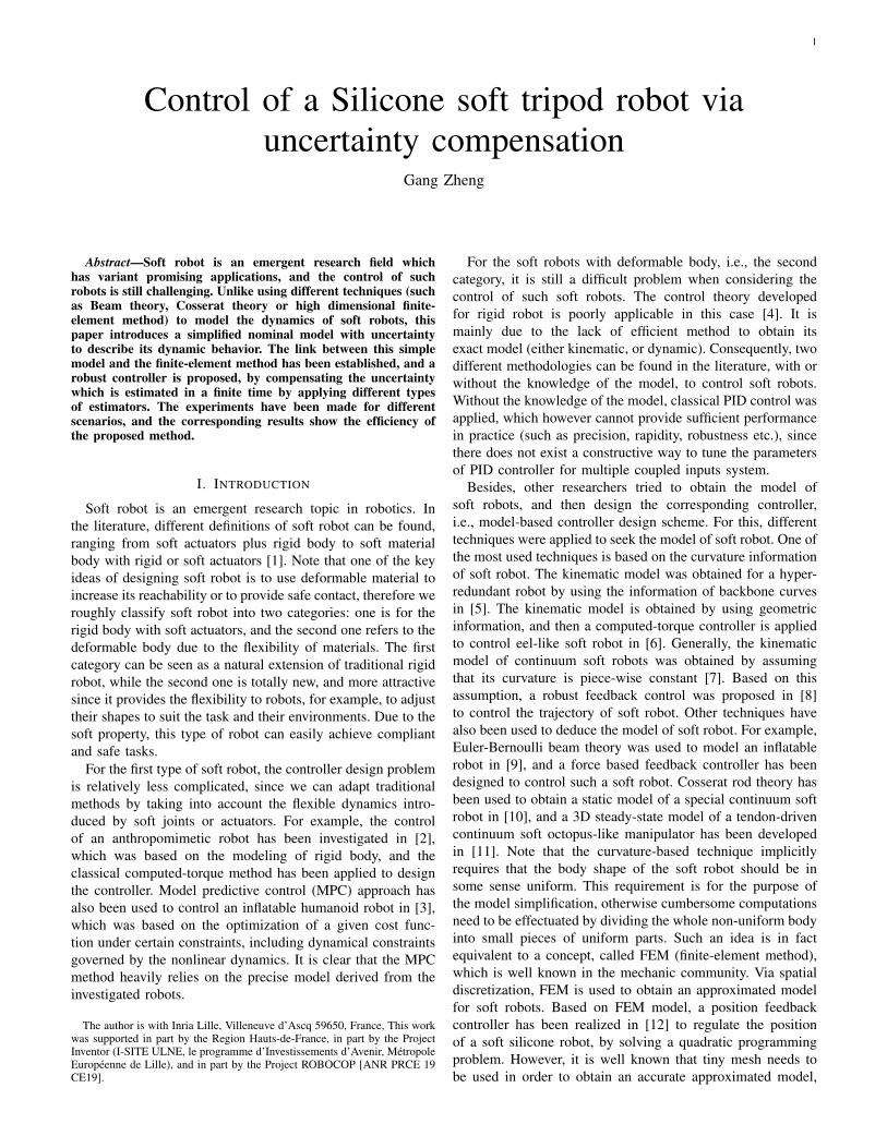
This paper investigates the position control of a 3D printedtripod-type soft robot which is made by silicone. The structureis described in the left picture of Fig. 1. This robot consistsof 3 flexible links AiBi for 1 ≤ i ≤ 3. On the top, a holeP with diameter 0.5cm is designed to hold small object. Theobjective is to displace the object in the hole. For this, threemotors are installed at points Ai in order to drive the linksAiBi for the purpose of moving the object on the top. Theoverall dimension of the soft robot is 15×15×9 cm, with 3D-printed hard parts and the molded shell-like silicone piece (the3 soft links). For the actuators, 3 SG90 servomotors are used,whose rotation angel can be controlled via MegaPi board.

1https://handsonsoftrobotics.lille.inria.fr

Fig. 1. Left: Tripod-type of 3D printed soft robot; Right: Its’ FEM model.

Due to the fact that the links are made by silicone, thusthey are flexible. Therefore, the exact kinematic and dynamicmodels of such a soft robot are quite difficult (or even impos-sible) to be obtained. One possible solution is to approximatethose exact models by using FEM. The basic idea of FEM isto discretize the space of robot by using finite number of fineelements to obtain its dynamical model.

Following the second law of Newton and FEM approach, wecan use the following nonlinear model to describe its behavior

M(q)q +D(q, q)q +K(q)q = HT (q)u (1)

where q ∈ Rn is the deformation of the nodes of the mesh,and u ∈ Rm represents the magnitude of the actuators. M(q)is mass matrix which is always invertible, D(q, q) is dampingmatrix, and K(q) represents stiffness matrix in order to modelthe internal forces of the soft robot, which depends on theconstitutive law (linear or nonlinear) of the soft material,characterized by the associated Young’s modulo and Poisonratio. H(q) represents the force directions (including actuatorsfrom the robot itself), and is rectangular operator, usuallysparse, as it has only non-zero values at the points where theactuators are applied. For the investigated soft robot, its FEMdiscretization is displayed in the right picture of Fig. 1, wherewe can see that the number of nodes is quite huge (1000 nodesin this figure), and it leads to high dimensional state of (1).

In the following, we would like to highlight that the FEM-based controller suffers from at least the following problems:

• The material of the real robot is never homogeneous, andis always spatially variant. This characteristic implies thatthe method of FEM will never give us a precise model;

• The number of nodes needs to be immense in orderto have an acceptable approximation for FEM, and therelation found by FEM depends on the huge matricesK(q) and H(q) in (1). This implies that FEM method iscomputationally expensive;

• The most important drawback is that: the control devel-oped based on FEM model might not be valid for the realsystem since FEM is only an approximated model.

In order to avoid the above mentioned inconveniences of FEM,this paper uses a simplified model as the nominal one todescribe the dynamics of P with respect to the control inputu, and the unmatched error will be then represented by theuncertain term. Based on this nominal model with unknownuncertainty, the objective of this paper is then to design robustcontroller to achieve position control of the object glued onthe top of the soft robot.

3

III. MODELING

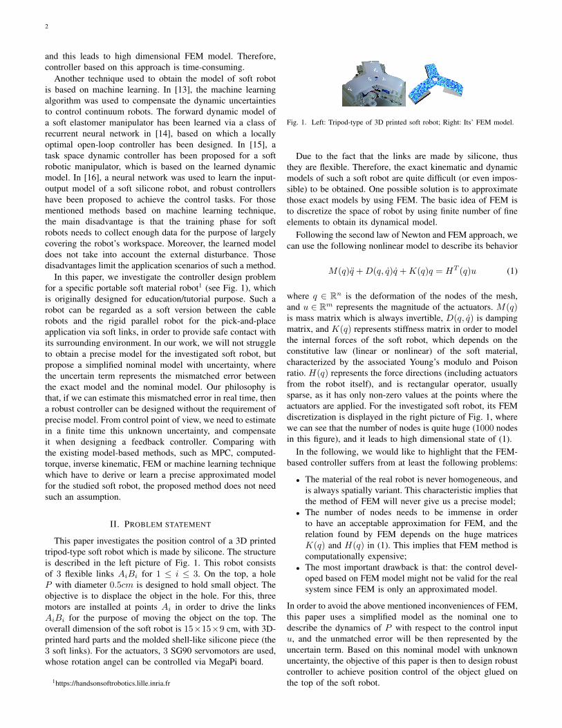
Before presenting the simplified nominal model for this softrobot, a global (inertial) frame needs to be chosen. In thispaper, we fix the x − z plane on the base, and choose thecenter point of the base as the origin O = (0, 0, 0), and assignone arbitrary motor on the axis x (

→OA1 as shown in Fig. 2).

Due to the symmetric form of this robot, the y-axis is upwardand perpendicular to the base.

Fig. 2. The chosen global frame fixed on the soft robot.

In this global frame, the coordinate of the top hole of thisrobot is noted as P = (x, y, z)T ∈ R3. Since we are interestedonly in the position control of the top hole, therefore the threemounted motors are enough to achieve this goal.

As we have mentioned in the last section that an exactdynamic model of the point P is quite difficult to be obtained,the following will introduce a simplified nominal linear modelwith uncertainty to model the dynamics of P .

A. Nominal model

According to the second law of Newton, similarly to (1),we know that the acceleration of an object is proportionalto the velocity (the effect of damping and viscous), to thedisplacement and to the external force. Obviously, the pa-rameters in front of the velocity, the displacement and theinputs might not be constant, like (1). But in practice, wecan choose a reasonable constant parameters (via the processof identification, which will be detailed in Section VII) torepresent its nominal model. Therefore, the nominal model todescribe the dynamics of the top hole for the studied soft robotis assumed to be of the following form:

P = Ap1 P +Ap2P +Bpu (2)

with Ap1 ∈ R3×3, Ap2 ∈ R3×3 and Bp ∈ R3×3. In theworkspace of the designed soft tripod robot, the matrix Bpshould be invertible, this is due to the fact that the positionof the top hole P is controllable [17]. The correspondingprocedure to identify the values of matrices Ap1 , Ap2 , and Bpwill be discussed in Section VII.

With the identified nominal model (2), we can then statethat the exact model can be written as

P = Ap1P +Ap2 P +Bpu+ d(t) (3)

where the term d(t) ∈ R3 represents the unmatched errorbetween the exact model and the identified nominal model(2). We would like to emphasize that, although the nominalmodel (2) was identified around certain operational posi-tions/trajectories, but the unmatched model parameters in Ap1 ,

Ap2 and Bp can be regarded as a resource of the uncertaintyd(t). In addition, the unmodeled nonlinearity can be alsoconsidered as another source of the uncertainty d(t). In thissense, we can say that the nominal uncertain model (3) enablesus to model precisely the movement of the soft robot.

B. Link to FEM

We can also make a link between the high dimensionalFEM model (1) and the low dimensional nominal uncertainmodel (3). For this, let us define P = Cq which representsthe position of the top hole of the soft robot. Then, we haveP = Cq with

q =M−1(q)[HT (q)u−D(q, q)q −K(q)q

]Hence we obtain P = f(q, q, · · · , u) which can be writtenin the nominal uncertain model (3) with

d(t) = f(q, q, · · · , u)−Ap1P −Ap2 P −Bpu

Such a formulation shows that the constitutive law, de-scribed by K(q) in (1), is hidden in d(t). We would like toemphasize that, in the framework of FEM, the constitutivelaw is normally assumed to be linear (i.e. elastic) for the sakeof modeling simplification. Such an assumption is no longerneeded when modeling the dynamic behavior of soft robot viathe nominal uncertain model (3), since the influence of theconstitutive law is now hidden in d(t) which will be estimatedand compensated in real time by the closed-loop controller.In other words, such a formulation enables us to treat morecomplicated constitutive law, such as hyper elastic one.

The objective of our work is then to design a robustcontroller to solve output regulation/tracking problem of (3)to a desired position Pr (not necessary to be constant, whichmight be time-varying), with the presence of the unknownuncertain term d(t).

IV. ESTIMATION OF UNCERTAINTIES

In the literature, there exists several approaches to solvethe output tracking problem for (3). One solution might bethe design of robust controller, such as sliding mode [18], todirectly eliminate the influence of bounded uncertainty, sincethe uncertainty d(t) affects system (3) in a matched way, i.e.,the uncertainty d(t) and the control u(t) are in the same line.Theoretically, sliding mode technique can achieve finite-timeconvergence. However, the gain of such a controller dependson the boundedness of d(t), thus the over-estimation of thisboundedness will lead to large gain. In addition, sliding modecontroller suffers from chattering phenomenon in practice.Another method to solve the output tracking problem for (3)is based on the idea to estimate the uncertainty d(t), and thencompensate it in the closed loop.

In this paper, we will adopt the second solution. To this aim,let us consider the dynamics of P defined in (3). Since Bpis invertible, therefore the uncertainty can be easily estimatedvia d(t) = P −Ap1P −Ap2 P . This formula shows that high-order derivatives of P are required to estimate the unknownuncertainty. Therefore, the following will recall some well-known differentiators to calculate high-order derivatives.

4

The simplest differentiator is the so-called high-gain differ-entiator [19]. Consider P as the signal for which we want tocalculate its high-order derivatives, the high-gain differentiatoris of the following form:

ξ1 = ξ2 − k1(ξ1 − P )· · ·

ξn−1 = ξn − kn−1(ξ1 − P )ξn = −kn(ξ1 − P )

(4)

Define ei(t) = ξi(t) − P (i−1)(t) where P (i−1)(t) representsthe (i − 1)th derivative of P (t). Then we can obtain thefollowing dynamics of observation error:

e1 = e2 − k1e1· · ·

en−1 = en − k2e1en = −kne1 − P (n)

(5)

By assuming that P (n) is bounded (which is always true inpractice), it has been proven in [19] that, with the choice ofthe following gains:[

k1 k2 . . . kn]=[l1ε

l2ε2 . . . ln

εn

](6)

where ε is a small positive parameter (thus ki is high gain)and li are positive constants which make the roots of sn +l1s

n−1 + · · · + ln−1s + ln = 0 having negative real parts,then the estimation error ei will decay to O(ε) after a shorttransient period. Consequently the high-order derivatives of Pcan be obtained as ξi ≈ P (i−1).

Note that the high-gain differentiator can only provideasymptotic convergence to a small neighborhood of the realderivative. In order to overcome this problem, the so-calledHOSM (High-order sliding mode) differentiator and HOMD(Homogeneous finite-time) differentiator are proposed, whichare of the following similar form:

ξ1 = ξ2 − k1pξ1 − Pyα· · ·

ξn−1 = ξn − kn−1pξ1 − Py(n−1)α−(n−2)ξn = −knpξ1 − Pynα−(n−1)

(7)

where payb = |a|bsign(a) and ki was chosen such thatthe roots of sn + k1s

n−1 + · · · + kn−1s + kn = 0 havingnegative real parts. Depending on different choices of α, thedifferentiator (7) is HOMD if α ∈ (n−1n , 1), and it representsa HOSM differentiator if α = n−1

n . Following the sameprocedure stated for high-gain differentiator, the dynamics ofobservation error becomes:

e1 = e2 − k1 de1cα· · ·

en−1 = en − kn−1 de1c(n−1)α−(n−2)

en = −kn de1cnα−(n−1) − P (n)

(8)

It has been shown in [20] that the observation error ei willconverge to zero in a finite time.

In other words, given the top hole position P of thesoft robot, HOSM and HOMD differentiators can preciselycalculate P and P in a finite time, i.e., ∃t ≥ Ts, such that

ξ1 = P , ξ2 = P and ξ3 = P . Therefore, the uncertainty termd(t) can be estimated as

d(t) = ξ3 −Ap1ξ1 −Ap2ξ2 (9)

V. ROBUST CONTROLLER DESIGN

For the nominal system with uncertainty (3), with uncer-tainty estimation method (9), we can then design the followingrobust controller

u = B−1p

[−d(t)−Ap1ξ1 −Ap2ξ2 + Pr +Kpe+Kde

](10)

where e = Pr − ξ1 and e = Pr − ξ2.

Theorem 1. For the robot described by (3), given a desiredtrajectory Pr(t), with the proposed uncertainty estimator (9),there exist Kd and Kp such that the robust controller (10) canasymptotically track Pr(t), i.e., limt→∞ ||P (t)− Pr(t)|| = 0.

Proof. For system (3), it is clear that the high-order derivativesof P should be bounded since P represents the position of thetop hole of the soft robot. Then, it has been proven in [18] that,for any initial condition ξi(t0), there always exists a settlingtime Ts such that for all t ≥ Ts we have ξi(t) = P (i−1)(t) for1 ≤ i ≤ n, where P (i−1) represents the (i−1)th derivative ofP with respect to time. In other words, after t ≥ Ts, we obtainthe exact estimation ξ1 = P , ξ2 = P and ξ3 = P . Accordingto (9), after t ≥ Ts, we can state that

d(t) = ξ3 −Ap1ξ1 −Ap2ξ2 = P −Ap1P −Ap2 P = d(t)

and the corresponding control as

u = B−1p

[−d(t)−Ap1P −Ap2 P + Pr +Kpe+Kde

]with e = Pr −P and e = Pr − P . Therefore, substituting thecontroller (10) back into the nominal uncertain system (3), wecan finally get the closed-loop system as follows:

P = Ap1P +Ap2 P +Bpu+ d(t)

= Pr +Kpe+Kde

The above equation can be then rewritten as e+Kde+Kpe =0. Note that this is a 3-dimensional totally decoupled 2-ordersystem, therefore we can always find the parameters Kd ∈ R3

and Kp ∈ R3 such that the closed-loop system is stable.A simple criteria to determine Kd and Kp is to satisfy the

following inequality:[0 I3×3

−Kp −Kd

]≺ 0

i.e., negative positive.By using the Lyapunov function V = 1

2eT e+ 1

2 eT e, we can

then have

V = eT e+ eT e = eT e− eTKde− eTKpe

= [e, e]T

[0 I3×3

−Kp −Kd

] [ee

]< 0

Therefore, we can conclude that limt→∞ ||e(t)|| = 0 whichimplies that limt→∞ ||P (t)− Pr(t)|| = 0.

5

VI. EXTERNAL PERTURBATION REJECTION

Another advantage of the proposed controller is the rejectionof external perturbation. To illustrate this characteristic, let usconsider the external perturbation added to the body of thesoft robot, noted as Fd(t), with the following assumption.

Assumption 1. It is assumed that the external perturbationFd(t) is bounded under which there exists a control u(t) suchthat the P (t) can still reach the desired position Pr.

This assumption is important for two reasons. Firstly, theexternal perturbation needs to be bounded which is alwaystrue in practice, otherwise the position P will tend to infinity.Secondly, even Fd(t) is bounded, there exist certain particularsituations such that P cannot, under the additional perturbationFd(t), reach the desired position Pr anymore. For example, ifFd(t) was opposite (but with the same magnitude) to u(t), thenP cannot be controlled in this case. In summary, Assumption 1is imposed for the purpose of guaranteeing the controllabilityof P to the desired position Pr.

Under Assumption 1, the external perturbation Fd(t) canalso be considered as an additional resource of d(t) in (3).This can be also interpreted by using FEM, whose model isof the following form:

M(q)q +D(q, q)q +K(q)q = HT (q)u+HF (q, t)Fd (11)

where HF (q, t) implies the directions/time where/when theexternal perturbation Fd(t) is applied. Following the sameprocedure in Section V, we obtain P = f(q, q, · · · , Fd, u)which can be again written as the nominal uncertain model(3) with d(t) = f(q, q, · · · , Fd, u)−Ap1P −Ap2 P −Bpu.

From the above analysis, we can conclude the robustnessof the proposed controller via the following result.

Theorem 2. For the soft robot described by (3), given a de-sired trajectory Pr(t), with external perturbation Fd satisfyingAssumption 1, there exist Kd and Kp such that the proposeduncertainty estimator (9) and the robust controller (10) canasymptotically track Pr(t), i.e., limt→∞ ||P (t)− Pr(t)|| = 0.

Proof. It is omitted since it is similar to that of Theorem 2.

VII. EXPERIMENT

In order to validate the proposed approach, we implementthe proposed uncertainty estimator (9) and the robust controller(10) to control the soft robot described in Fig. 1.

A. Experimental setup

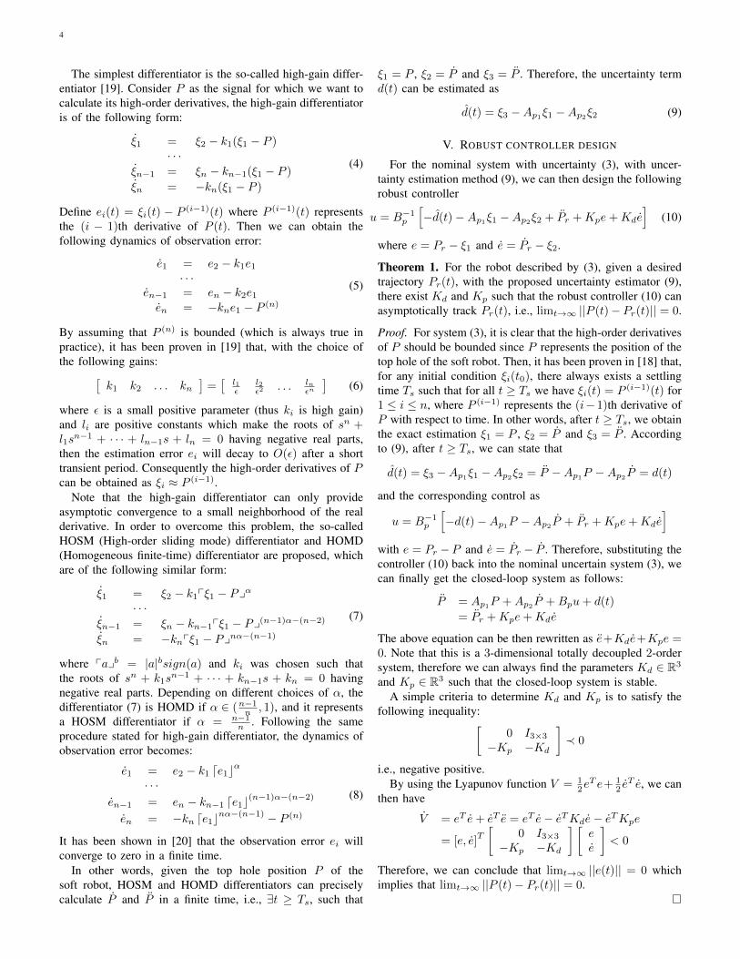
In the experiment, the robot described in Fig. 1 was printedby 3D printer with silicone. In our test, we are interestedin controlling the top hole position of such a silicone robot.Therefore, three markers are glued on the top of the robot (seeFig. 3 (left)). In order to capture in real time the position ofthe center of these three markers, an OptiTrack system with 4ultra-red cameras is installed around this robot. These camerasare fixed above the robot and can localize the center positionof these three markers with high precision (in millimeter).

We would like to remark two important facts. First, theminimal configuration (i.e., 4 cameras and 3 markers) is

Fig. 3. Experimental setup and external perturbations. Left: Soft robot with3 markers for OptiTrack tracking; Center: Temporary perturbation was addedby touching the soft link with pen; Right: Permanent perturbation was addedby gluing an extra material on the soft link.

used during our experiment for easily determining the masscenter of all markers, but more markers and cameras canbe used for redundancy to account for occlusions whichcould affect tracking error. Secondly, the proposed controlleris independent of the types of sensors we used, if we canmeasure or estimate the position of the top hole in real time.In other words, different types of sensors (external one suchas OptiTrack, or internal one such as air-flow measurement[21]) might be used to measure the position of the top hole,depending on the specific application scenarios.

B. Experimental results

To show the efficiency of the proposed approach, differentexperiments are made, respectively to stabilize P = (x, y, z)to a desired position (xr, yr, zr) (constant or time-varying),without and with external perturbations.

1) Identification of nominal model: In order to identifythe values of matrices Ap1 , Ap2 and Bp in (2), classicalidentification process has been effectuated for this robot.Precisely, we applied the following inputs

u(t) =

1.5 + sin 0.15t1 + sin 0.1t1.3 + sin 0.85t

× 20, for 0 < t ≤ 10

to the three motors, and recorded the corresponding po-sition P (t) via OptiTrack system. Then HOMD differ-entiator in (7) was used to calculate P (t) and P (t).Thus, the nominal model can be written as P (t) =[Ap1 , Ap2 , Bp] [P

T (t), PT (t), uT (t)]T . By using Least-squaremethod, we can then identify the matrices Ap1 , Ap2 and Bp,whose values are:

Ap1 =

−0.10 −0.11 −0.200.35 −0.21 −0.200.19 0.29 −0.17

Ap2 =

−0.13 0.12 −0.67−0.33 0.19 0.15−0.37 −0.29 0.59

Bp =

0.86 0.34 0.04−0.25 0.73 −0.32−0.37 0.82 0.41

2) Stabilization to a desired position on y-axis: In order to

show the advantage of the proposed controller, we comparedthe results with respect to a simple PID controller.

Fig. 4 (left) shows the position errors between P and thedesired position by using classical PID controller. It can be

6

0 500 1000 1500 2000

ms

-5

0

5

10

15

20

25

30

35

40

mm

ex

ey

ez

0 500 1000 1500 2000

ms

-20

-10

0

10

20

30

40

50

mm

ex

ey

ez

Fig. 4. Stabilization error to a desired position via the PID controller (left)and via controller (10) (right).

seen that PID controller can realize the task around 1000ms.Fig. 4 (right) depicts the experimental result in the samesettings, but by using the proposed controller. It is clear that theproposed controller makes the robot converging to the desiredposition faster, around 400ms. This experiment highlights thefast convergence property of the proposed controller withrespect to classical PID controller, which is logical sincePID controller does not use any information of the model.It is worth noting that the convergence speed can be tunedfor PID controller by choosing different parameters. Such atuning procedure is relatively easy for SISO (Single InputSingle Output) system, but generally there does not exista constructive process to tune those parameters for MIMO(Multi Inputs Multi Outputs) system, which is the case forthe studied soft robot: we have 3 coupled inputs, therefore 9coupled gains need to be carefully tuned for different operatingpoints. For the studied robot, it is clear that different motorhas different contribution to move the position of the tophole. Due to this coupling fact, i.e., the modification of onecontroller will influence the other one, the tuning procedure istime-consuming and will lead to the so-called gain-schedulingcontrol scheme.

3) Stabilization to a desired position in different zones: Inorder to show the feasibility of the proposed controller, in thisexperiment we will stabilize the robot to 3 different zones (seeFig. 2 for the definition of zones). Figs. 5-7 show the positionerrors when stabilizing the robot to a desired constant positionlocated in Zone 1, Zone 2 and Zone 3, respectively. We cansee that the proposed controller can achieve the task for allthree zones, with a fast convergence speed.

0 500 1000 1500 2000

ms

-5

0

5

10

15

20

mm

ex

ey

ez

Fig. 5. Stabilization error to a desired position in Zone 1 via controller (10).

4) With external perturbation: In order to show the robust-ness of the proposed method, two types of perturbations areadded to the robot (see the center and right picture in Fig. 3

0 500 1000 1500 2000

ms

-15

-10

-5

0

5

10

15

20

mm

ex

ey

ez

Fig. 6. Stabilization error to a desired position in Zone 2 via controller (10).

0 200 400 600 800 1000

ms

-10

-5

0

5

10

15

20

mm

ex

ey

ez

Fig. 7. Stabilization error to a desired position in Zone 3 via controller (10).

). The first one is temporary, where we manually perturb therobot with a pen and then release it. Fig. 8 (left) shows theexperimental results. We can see that the proposed controllercan keep the robot on the desired position when such anexternal temporary perturbation is presented and vanished.

The second type of perturbation is permanent. We manuallyglue an extra material on the body of soft robot, for the pur-pose of mimicking an external perturbation which is presentpermanently. As shown in Fig. 8 (right), the proposed approachcan reject this perturbation, even it is permanent.

From those experimental results, it is clear that the proposedrobust controller can successfully drive the point of interest(the center of three markers glued on the top of robot) to adesired constant position in different zones, and it is robustwith respect to external perturbation.

5) Trajectory tracking: For the purpose of tracking a time-varying trajectory, we define the following references

Pr(t) =

xr(t)yr(t)zr(t)

=

10 sin 0.5t− 1010 cos 0.6t+ 2010 sin 0.8t+ 10

0 500 1000 1500 2000 2500 3000

ms

-15

-10

-5

0

5

10

15

20

25

30

mm

ex

ey

ez

0 200 400 600 800 1000 1200 1400 1600 1800

ms

-10

-5

0

5

10

15

20

25

mm

ex

ey

ez

Fig. 8. Robustness with respect to an external temporary perturbation (left)and an external permanent perturbation (right).

7

Moreover, in order to highlight the efficiency of the uncer-tainty compensation, two tests are made, respectively with theestimation and compensation of the uncertainty and without it.The relative results are shown in Fig. 9, where we can see that,the controller (10) without the compensation of the uncertaintyd(t) cannot achieve the trajectory tracking task. Comparedto the trajectory reference, it has a bounded but oscillatorytendency. This phenomenon can be interpreted as follows:the uncompensated term d(t), which is used to catch theunmatched modeling error between the linear nominal modeland the real one, might be nonlinear in some neighborhoodsof the reference, therefore the robot cannot converge to thereference by the controller (10) without the uncertainty com-pensation. Conversely, when integrating the compensation ofthis uncertainty, the proposed controller can successfully trackthe defined time-varying trajectory. This experiment clearlyshows that the estimation and compensation of the uncertaintyterm d(t) plays an important role of the proposed controller.

0 500 1000 1500 2000

ms

-20

-10

0

10

20

30

40

mm

Fig. 9. Performance comparisons for the proposed control without and withthe uncertainty compensation for tracking time-varying references.

VIII. CONCLUSION

In this paper, we proposed to use a simplified linear nominalmodel with uncertainty to describe the dynamics of soft robots.By analyzing the disadvantage of classical FEM approach tomodel soft robot, we showed the feasibility of the proposedapproach by linking the FEM model to the proposed one.Then, the problem of position control of soft robot is convertedto investigate the estimation of uncertainty and the design ofrobust controller by compensating the estimated uncertainty. Inthis paper, different types of uncertainty estimators have beendiscussed. Also, the scenario with external perturbation hasbeen analyzed for the purpose of highlighting the robustness ofthe proposed controller. Finally, different types of experimentshave been carried out, including the stabilization to a constantor time-varying desired position in different zones, and thecase with external perturbation. The experimental results showthat the proposed approach is efficient, and robust to achieveposition control of the investigated soft robot.

REFERENCES

[1] D. Trivedi, C. D. Rahn, W. M. Kier, and I. D. Walker, “Soft robotics:Biological inspiration, state of the art, and future research,” Appl. BionicsBiomechanics, vol. 5, no. 3, pp. 99–117, 2008.

[2] S. Wittmeier, C. Alessandro, N. Bascarevic, K. Dalamagkidis, D. Dev-ereux, A. Diamond, M. Jäntsch, K. Jovanovic, R. Knight, H. G. Marques,P. Milosavljevic, B. Mitra, B. Svetozarevic, V. Potkonjak, R. Pfeifer,A. Knoll, and O. Holland, “Toward anthropomimetic robotics: Devel-opment, simulation, and control of a musculoskeletal torso,” ArtificialLife, vol. 19, no. 1, pp. 171–193, 2013.

[3] C. M. Best, M. T. Gillespie, P. Hyatt, L. Rupert, V. Sherrod, and M. D.Killpack, “A new soft robot control method: Using model predictive con-trol for a pneumatically actuated humanoid,” IEEE Robotics AutomationMagazine, vol. 23, no. 3, pp. 75–84, Sept 2016.

[4] C. Laschi and M. Cianchetti, “Soft robotics: new perspectives for robotbodyware and control,” Frontiers in bioengineering and biotechnology,vol. 2, p. 3, 2014.

[5] G. S. Chirikjian and J. W. Burdick, “A modal approach to hyper-redundant manipulator kinematics,” IEEE Transactions on Robotics andAutomation, vol. 10, no. 3, pp. 343–354, 1994.

[6] F. Boyer, M. Porez, and W. Khalil, “Macro-continuous computed torquealgorithm for a three-dimensional eel-like robot,” IEEE Transactions onRobotics, vol. 22, no. 4, pp. 763–775, 2006.

[7] D. B. Camarillo, C. R. Carlson, and J. K. Salisbury, “Configurationtracking for continuum manipulators with coupled tendon drive,” IEEETransactions on Robotics, vol. 25, no. 4, pp. 798–808, Aug 2009.

[8] C. Della Santina, R. K. Katzschmann, A. Bicchi, and D. Rus, “Dynamiccontrol of soft robots interacting with the environment,” 2018.

[9] J. B. M. Siddharth Sanan and C. G. Atkeson, “Robots with inflatablelinks,” in The 2009 IEEE/RSJ International Conference on Inte lligentRobots and Systems October 11-15, 2009 St. Louis, USA. IEEE, 2009.

[10] B. A. Jones, R. L. Gray, and K. Turlapati, “Three dimensional staticsfor continuum robotics,” in 2009 IEEE/RSJ International Conference onIntelligent Robots and Systems, Oct 2009, pp. 2659–2664.

[11] F. Renda, M. Cianchetti, M. Giorelli, A. Arienti, and C. Laschi, “A3d steady-state model of a tendon-driven continuum soft manipulatorinspired by the octopus arm,” Bioinspiration & biomimetics, vol. 7, no. 2,p. 025006, 2012.

[12] Z. Zhang, J. Dequidt, and C. Duriez, “Vision-Based Sensing of ExternalForces Acting on Soft Robots Using Finite Element Method,” IEEERobotics and Automation Letters, vol. 3, no. 3, pp. 1529 – 1536, Feb.2018.

[13] D. Braganza, D. M. Dawson, I. D. Walker, and N. Nath, “A neuralnetwork controller for continuum robots,” IEEE transactions on robotics,vol. 23, no. 6, pp. 1270–1277, 2007.

[14] A. D. Marchese, R. Tedrake, and D. Rus, “Dynamics and trajectoryoptimization for a soft spatial fluidic elastomer manipulator,” TheInternational Journal of Robotics Research, vol. 35, no. 8, pp. 1000–1019, 2016.

[15] T. G. Thuruthel, E. Falotico, F. Renda, and C. Laschi, “Learning dynamicmodels for open loop predictive control of soft robotic manipulators,”Bioinspiration & biomimetics, vol. 12, no. 6, p. 066003, 2017.

[16] G. Zheng, Y. Zhou, and M. Ju, “Robust control of a silicone soft robotusing neural networks,” ISA Transactions, accepted, 2019.

[17] G. Zheng, O. Goury, M. Thieffry, A. Kruszewski, and C. Duriez,“Controllability pre-verification of silicon soft robots based on finite-element method,” in Robotics and Automation (ICRA), 2019 IEEEInternational Conference on.

[18] A. Levant, “Sliding order and sliding accuracy in sliding mode control,”International journal of control, vol. 58, no. 6, pp. 1247–1263, 1993.

[19] H. K. Khalil, “High-gain observers in nonlinear feedback control,” in2008 International Conference on Control, Automation and Systems.IEEE, 2008, pp. xlvii–lvii.

[20] Y. Wang, G. Zheng, D. Efimov, and W. Perruquetti, “Differentiatorapplication in altitude control for an indoor blimp robot,” InternationalJournal of Control, pp. 1–10, 2018.

[21] S. E. Navarro, O. Goury, G. Zheng, T. M. Bieze, and C. Duriez,“Modeling novel soft mechanosensors based on air-flow measurements,”IEEE Robotics and Automation Letters, vol. 4, no. 4, pp. 4338–4345,2019.